license buyback programs in commercial fisheries: an...
TRANSCRIPT

LICENSE BUYBACK PROGRAMS IN COMMERCIAL FISHERIES: AN
APPLICATION TO THE SHRIMP FISHERY IN THE GULF OF MEXICO
A Dissertation
by
AARON T. MAMULA
Submitted to the Office of Graduate Studies of Texas A&M University
in partial fulfillment of the requirements for the degree of
DOCTOR OF PHILOSOPHY
May 2009
Major Subject: Agricultural Economics

LICENSE BUYBACK PROGRAMS IN COMMERCIAL FISHERIES: AN
APPLICATION TO THE SHRIMP FISHERY IN THE GULF OF MEXICO
A Dissertation
by
AARON T. MAMULA
Submitted to the Office of Graduate Studies of Texas A&M University
in partial fulfillment of the requirements for the degree of
DOCTOR OF PHILOSOPHY
Approved by:
Co-Chairs of Committee, Richard T. Woodward Wade L. Griffin Committee Members, H. Alan Love W. Douglass Shaw Head of Department, John P. Nichols
May 2009
Major Subject: Agricultural Economics

iii
ABSTRACT
License Buyback Programs in Commercial Fisheries: An Application to the Shrimp
Fishery in the Gulf of Mexico. (May 2009)
Aaron T. Mamula, B.A., Oregon State University;
M.A, Southern Methodist University
Co-Chairs of Advisory Committee: Dr. Richard T. Woodward Dr. Wade L. Griffin
This dissertation provides a thorough analysis of the costs associated with, and
efficacy of, sequential license buyback auctions. I use data from the Texas Shrimp
License Buyback Program – a sequential license buyback auction – to estimate the
effects of a repeated game set-up on bidding behavior. I develop a dynamic econometric
model to estimate parameters of the fisherman’s optimal bidding function in this auction.
The model incorporates the learning that occurs when an agent is able to submit bids for
the same asset in multiple rounds and is capable of distinguishing between the
fisherman’s underlying valuation of the license and the speculative premium induced by
the sequential auction. I show that bidders in the sequential auction do in fact inflate
bids above their true license valuation in response to the sequential auction format.
The results from our econometric model are used to simulate a hypothetical
buyback program for capacity reduction in the offshore shrimp fishery in the Gulf of
Mexico using two competing auction formats: the sequential auction and the one-time
iv
auction. I use this simulation analysis to compare the cost and effectiveness of
sequential license buyback program relative to one-time license buyback programs. I
find that one-time auctions, although they impose a greater up-front cost on the
management agency – are capable of retiring more fishing effort per dollar spent then
sequential license buyback programs. In particular, I find one-time license buyback
auctions to be more cost effective than sequential ones because they remove the
possibility for fishermen to learn about the agency’s willingness to pay function and use
this information to extract sale prices in excess of the true license value.

v
ACKNOWLEDGEMENTS
This research was funded by a grant from the National Marine Fisheries Service
and would not have been possible without their support. I would like to thank Thomas
Osang and Kevin Marshall who encouraged me to pursue economic research beyond my
master’s thesis. I would also like to thank my committee members, Douglass Shaw and
Alan Love, for their helpful comments on this dissertation. My major advisors, Rich
Woodward and Wade Griffin deserve special acknowledgement, for their guidance and
patience.
In addition to academic support, I received social support from an excellent
group of friends who made my time at Texas A&M memorable – Heather, Brandon,
Levan, Dave, Alex, Chris, Erin, Jamie, Lindsey, and all of the girls, past and present, of
the Texas A&M Women’s Club Soccer Team. You all made my time in College Station
memorable.
I would like to thank my brothers, Phil and Rob, for their support and friendship.
Finally, I dedicate this dissertation to my parents, Patty and Greg, who have always
supported me, unconditionally, in all things.

vi
TABLE OF CONTENTS
Page
ABSTRACT .............................................................................................................. iii
ACKNOWLEDGEMENTS ...................................................................................... v
TABLE OF CONTENTS .......................................................................................... vi
LIST OF FIGURES................................................................................................... viii
LIST OF TABLES .................................................................................................... x
CHAPTER
I INTRODUCTION................................................................................ 1
II A BRIEF SURVEY OF THE THEORETICAL ANALYSIS OF AUCTIONS.................................................................................... 6 Introduction .................................................................................... 6 Benchmark Auction........................................................................ 7 Sequential Auctions........................................................................ 12
Summary ........................................................................................ 19 III LESSONS FROM THE TEXAS INSHORE SHRIMP FISHERY...... 21
Introduction .................................................................................... 21 Literature ........................................................................................ 22 A Background on the Texas Shrimp License Buyback.................. 25
Data ................................................................................................ 30 Buyback Outcomes ........................................................................ 33 Auction Behavior ........................................................................... 41 Summary of Lessons from the Texas Shrimp License Buyback ... 57 IV AN EMPIRICAL MODEL OF BIDDING IN SEQUENTIAL AUCTIONS.......................................................................................... 60 Introduction .................................................................................... 60 Literature Relevant to the Estimation of Dynamic Decision Processes ......................................................................... 61
vii
CHAPTER Page Model ............................................................................................. 63 Estimation....................................................................................... 74 Results ............................................................................................ 81 Model Validation............................................................................ 84 Discussion ...................................................................................... 104 Summary of Empirical Work ......................................................... 106 V A COST-BENEFIT ANALYSIS OF SEQUENTIAL VERSUS ONE-TIME BUYBACK AUCTIONS................................................. 109 Introduction .................................................................................... 109 Important Terms and Concepts ...................................................... 111 Methodology .................................................................................. 113 A GBFSM Introduction.................................................................. 114 Important Assumptions of the Simulation Model .......................... 125 Scenario Analysis ........................................................................... 129 Results ............................................................................................ 131 Summary of Simulation Work ....................................................... 169 VI SUMMARY AND CONCLUSIONS.................................................. 170
NOMENCLATURE.................................................................................................. 175
REFERENCES.......................................................................................................... 176
APPENDIX A ........................................................................................................... 180
VITA ......................................................................................................................... 181
viii
LIST OF FIGURES
FIGURE Page
3.1 Single License Decision Tree..................................................................... 29 3.2 Catch per Unit Effort for the TX Inshore Shrimp Fishery 1995 - 2004..... 38 3.3 Vessel Length Distribution by Age of Owner in 1996............................... 45 3.4 TX License Buyback Auction Round 1 Bids ............................................. 51 3.5 TX License Buyback Auction Round 6 Bids ............................................. 52 3.6 TX License Buyback Auction Round 14 Bids ........................................... 52
3.7 Returns to Rejecting an Offer After It Was Granted.................................. 56
4.1 Prior and Posterior Expected Probabilities in the Sequential Bidding Problem When a Bid Is Granted....................... 69 4.2 Prior Subjective Distribution for RPLo = $4,000 and RPHi = $10,000..... 70
4.3 Flow of the Econometric Model................................................................. 77
4.4 Average Bid and Price by Round in the TX Shrimp License Buyback Auction ....................................................... 82 4.5 Actual and Predicted 1st Bids ..................................................................... 87
4.6 Actual and Predicted 2nd Bids .................................................................... 88
4.7 Objective Function Values in the RPLo Dimension .................................. 89
4.8 Objective Function Values in the RPSpread Dimension ........................... 89
4.9 Numerical Derivatives of the Implied Likelihood Function Around the Optimum ................................................................................. 95 4.10 Objective Function Values in the y1 Dimension........................................ 99
4.11 Objective Function Values in the y2 Dimension........................................ 99
ix
FIGURE Page
4.12 Prediction Error by Vessel Length ............................................................. 101
4.13 Prediction Error by Shrimp Price ............................................................... 102
4.14 Sample Observations and Price.................................................................. 102
4.15 Implied R Values for Average Vessel ........................................................ 104
4.16 Average Speculative Premium by Round for All Vessels ......................... 105
4.17 Average Speculative Premium by Round and Length Class...................... 106
5.1 An Illustration of the General Bioeconomic Fisheries Simulation Model ....................................................................................... 119 A.1 License Holder Age by Round of the TX Shrimp License Buyback ......... 180
A.2 Average Vessel Length of TX Inshore Shrimp Fleet by Auction Round .. 180

x
LIST OF TABLES
TABLE Page 3.1 Selected US Fisheries Buyback Programs ................................................. 34 3.2 License Purchases by Round for the TX Program ..................................... 36 3.3 Key Indicators of the Health of the TX Inshore Shrimp Fishery ............... 39
3.4 Probit Regression to Explain Auction Participation .................................. 47 3.5 OLS Estimation of the Fisherman’s Bidding Function.............................. 48 4.1 Final Parameter Grids and Estimates ......................................................... 83 4.2 Mean Absolute Error by Bid Number ........................................................ 86 4.3 Standard Errors of the Parameter Estimates............................................... 98 5.1 Four Gulf Regions of Shrimp Landings in the General Bioeconomic Fisheries Simulation Model ................................................. 115 5.2 Sample of a Simulated Distribution of Bids............................................... 123 5.3 Baseline Scenario Results for Large Vessels ............................................. 133 5.4 Baseline Scenario Results for Small Vessels ............................................. 134 5.5 Baseline Landings and Catch per Unit Effort Summary for Large Gulf Vessels ............................................................................... 135 5.6 Gulfwide Sequential Buyback Snapshot (Large Gulf Vessels).................. 136 5.7 Gulfwide Sequential Buyback Annual Rents (7% Discount Rate) ............ 137 5.8 Gulfwide One-time Buyback Snapshot (Large Gulf Vessels) ................... 138 5.9 Gulfwide One-time Buyback Rents ........................................................... 139 5.10 Gulfwide Sequential Buyback and One-time Buyback Auction Comparison ................................................................................................ 140

xi
TABLE Page 5.11 Gulfwide Sequential Buyback Auction Average Price by Round ............. 141 5.12 Aggregate Effects – Regional Sequential Buyback vs. Gulfwide Sequential Buyback Programs ................................................................... 144 5.13 Rents Under Sequential Buyback Programs .............................................. 145 5.14 Aggregate Effects – Regional One-time Buyback vs. Gulfwide One-Time Buyback .................................................................................... 147 5.15 Rent Comparison – Gulfwide One-time Buyback vs. Regional One-Time Buyback .................................................................................... 149 5.16 Expenditures by Region ($1,000s) ............................................................. 151 5.17 Change in Catch per Unit Effort by Region (% Change)........................... 153 5.18 Total Rents Above Baseline (Present Value, $1,000) ................................ 154 5.19 Regional Sequential Buyback Program’s Change in Landings with Respect to Change in Effort (Change in lbs/Change in Days-Fished) ....... 158 5.20 Landings and Effort Comparison for Regions 2 and 4............................... 159 5.21 Landings and Effort for Inshore Fisheries Under Regional Sequential Buyback.................................................................................... 160 5.22 Four Program Ranking – Rank in Parentheses........................................... 162 5.23 Marginal Benefit and Cost to Purchase One Additional Vessel for Gulfwide Sequential Buyback Program ............................................... 166 5.24 Change in Rents per Dollar Spent for Sequential Buyback Programs....... 168
1
CHAPTER I
INTRODUCTION
Overfishing is currently a serious concern for fisheries managers in the US and
around the globe. In the March 2008 publication of the Fish Stock Sustainability Index
(FSSI), the National Marine Fisheries Service reported that overfishing was occurring in
22% of US stocks. The FSSI also reports that 27% of domestic stocks are overfished. In
their 2006 report, “State of the World Fisheries and Aquaculture (SOFIA),” the Food and
Agriculture Organization of the United Nations reported that 25% of the world’s fish
stocks were overexploited.
The damage done to fish stocks through overfishing has a profound impact on
marine ecosystems as well as human welfare. Many coastal communities rely on
commercial fishing to provide jobs and income. When stocks become overfished the
result is often economic hardship for these communities. In addition to supporting the
commercial fishing industry, healthy marine ecosystems also provide benefits to
recreational fishermen and ecotourists.
In recognition of the importance of marine resources and the failure of open
access policies to provide healthy marine environments, fisheries management has
emerged as an important topic among resource economists. The literature in resource
and environmental economics now contains extensive discussions on the relative
strengths of the various policies used to manage marine resources. In this dissertation I
This dissertation follows the style of Marine Resource Economics.

2
focus on one particular class of fisheries management policies: buyback programs.
Domestically, buyback programs have been used in the Northeast ground fish
fishery, the Columbia River salmon fishery in Oregon and Washington and the Bearing
Sea/Aleutian Islands (BSAI) crab fishery in Alaska among others. Internationally,
buyback programs have been used in the Australian Northern Prawn fishery, British
Columbia salmon fishery, and Norwegian purse seine fishery (case studies of these and
other buyback programs can be found in Holland, Gudmundsson, and Gates 1999 and
Curtis and Squires 2007).
In addition to being significant in number, many buyback programs come with a
significant price tag. In 2004 the vessel buyback program carried out in the BSAI crab
fishery spent over $97 million. The Texas Inshore Shrimp License Buyback Program,
which will be discussed in detail in this dissertation, spent over $8 million in its first 7
years.
Buyback programs have traditionally found favor with fisheries managers
because of their ability to address a range of management goals. In addition to providing
capacity reduction for the purpose of reducing overfishing, buyback programs may be
designed to address the problem of by catch within a fishery or used as a way to
distribute disaster relief funds. Holland et al. (1999) identify three general policy aims
important to fisheries managers which buyback programs may be designed to address: 1)
conservation of fish stocks, 2) improvement of economic efficiency through fleet
rationalization, and 3) providing transfer payments to the fishing industry. Because of

3
their ability to address biological, economic, and social goals, buyback programs will
likely continue to find a place in the manager’s toolkit.
Although the economic literature on buyback programs is well developed and
contains a wealth of case studies, there seems to be a shortage of empirical work
addressing the question of how important design issues impact the efficacy of the
program. In this dissertation I will analyze the influence that auction format has on the
effectiveness of buyback programs. Given their popularity with fisheries managers and
the financial commitment required to run one successfully, it is crucial to have a
thorough understanding of how agents respond to the incentives created by buyback
programs and the bearing this behavior has on program success.
The principal objectives of this dissertation are to develop an empirical model of
bidding in a sequential buyback auction and, using results from this model, simulate
sequential and one-time buyback programs for capacity reduction in the Gulf of Mexico
Shrimp Fishery. The overriding goal of our study is to analyze the cost and effectiveness
of sequential buyback auctions relative to one-time buyback auctions. I approach this
goal in the following manner:
I first develop an econometric model of bidding under a sequential auction. The
parameters of this model allow us to distinguish the license holder’s true reservation
price and, by comparing this underlying value with actual bids, estimate the amount by
which the bidder inflates his or her bid in order to take advantage of the sequential
auction structure. I term this bid inflation the speculative premium. I then use data from
the Texas Inshore Shrimp License Buyback Program – a long running sequential auction

4
– to estimate the parameters of the license holder’s bidding function and the implied
speculative premium.
I use our econometric findings to help solve a particular resource management
problem – that of optimal design of a buyback auction. By simulating 2 hypothetical
buyback policies for capacity reduction of the commercial shrimp fishing fleet in the
Gulf of Mexico, I provide a thorough evaluation of the costs and effectiveness of
sequential buyback programs (SBs) relative to one-time buyback programs (OTBs).
The remainder of this dissertation is organized as follows. Chapter II will
provide a thorough literature review on auctions. In this chapter, I discuss the current
economic literature on auction theory and estimation of models using auction data. One
of the contributions of this dissertation is the development of a dynamic model capable
of incorporating the learning that occurs in sequential auctions. Our auction literature
review helps emphasize this contribution by presenting current approaches to modeling
auctions.
Chapter IV contains the development of our formal econometric model and
estimation results. I believe that an intriguing feature of the SB auction is that bidders
have an incentive to bid above their true valuation. In the event that a bid is not accepted
in the current period, the bidder will have another chance to participate in the auction
again next period. This fact leads bidders to attach a speculative premium to the true
value of the license. In Chapter IV I propose an econometric model capable of
estimating this speculative premium and distinguishing it from the underlying value of
the license.
5
In Chapter V I use our econometric results to inform a simulation model to
compare SB auctions with OTB auctions. Chapter V uses parameter estimates from our
econometric model to predict bidding behavior for a hypothetical SB auction for capacity
reduction in the Gulf of Mexico’s offshore shrimp fishery, including the Exclusive
Economic Zone (EEZ). I then simulate an alternative policy path using a OTB program
to buyback licenses in order to compare the results of these two auction forms.
Finally, concluding remarks will appear in Chapter VI. In this chapter I will
provide a summary of important results and discuss some directions for future research
in the area of license buyback programs.
6
CHAPTER II
A BRIEF SURVEY OF THE THEORETICAL ANALYSIS OF AUCTIONS
Introduction
The Texas Inshore Shrimp License Buyback Program is structured as a first-
price, sealed-bid auction, which has been conducted at least once a year since its
inception in 1996. In order to appreciate the contributions of the particular econometric
model developed in Chapter IV it is important to understand how economists have
traditionally approached auction data.
The subject of auctions has a rich history in the economics literature. In
particular, because they can serve as a price discovery mechanism for goods which lack
other well-defined markets, auctions are especially important in resource and
environmental economics, where non-market valuation plays a critical role. Though
there are many auction issues relevant to the field of resource economics in general, I
focus this literature review on a particular topic germane to our principal objectives: the
theoretical foundations of optimal bidding.
I begin by presenting some standard results for simple auction forms then expand
our review to include results from more complicated auction forms. The remainder of
this chapter will be organized as follows: first I present the derivation of optimal bidding
functions for a benchmark auction. Next, I review some generalizations of those results
which apply more closely to our license buyback auction. Then I move away from game
theory-based models and discuss learning in sequential auctions. Finally, I discuss some
7
literature on dynamic specifications for sequential competitive bidding and relate this
literature to our model.
Benchmark Auction
As with many empirical studies using auction data, our challenge is to use
observed data on bids to get some information on license holder’s private values.
Traditional empirical work has relied heavily on auction theory to provide a closed form
expression for optimal bidding strategies. These bidding functions relate observed bids
to unobserved values and, it is through these functions, that researchers have typically
derived information about private valuations. Although there are a number of thorough
surveys on optimal bidding in the literature (Milgrom and Weber 1982; Milgrom 1985;
Wilson 1987; Milgrom 1989), in the following section I will focus on the presentation of
McAfee and McMillian (1987).
McAfee and McMillan show that a Nash Equilibrium for a first-price, sealed-bid
auction can be found by maximizing the expected payoffs of an arbitrary bidder. In this
section I present the technical details of this approach as they are important for
understanding theoretically consistent bidding functions in general. I will also show that
this approach generalizes to the bidding functions for auctions which may violate one or
more of the four assumptions presented below. The simplest case is what the authors
refer to as the benchmark model. The benchmark model imposes the following four
assumptions:
8
1. The bidders are risk neutral.
2. The independent-private-values assumption applies. This means that each bidder
has his own value for the object and that this value is independent of other
bidders’ values.
3. The bidders are symmetric. This assumption requires that all private values come
from a single distribution.
4. Payment is a function of bids alone. A common violation of this assumption is
the case where royalties are required of the winning bidder.
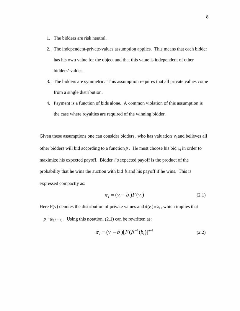
Given these assumptions one can consider bidder i , who has valuation iv and believes all
other bidders will bid according to a function . He must choose his bid ib in order to
maximize his expected payoff. Bidder si' expected payoff is the product of the
probability that he wins the auction with bid ib and his payoff if he wins. This is
expressed compactly as:
)()( iiii vFbv (2.1)
Here F(v) denotes the distribution of private values and ii bv )( , which implies that
.)(1ii vb Using this notation, (2.1) can be rewritten as:
11 )](()[( niiii bFbv (2.2)

9
In the equation above, n represent the number of bidders. Each bidder chooses his bid to
maximize expected payoff, so he chooses ib to satisfy the first order condition that
.0
i
i
b
Next one takes the total differential of i with respect to iv :
i
i
i
i
i
i
i
i
i
i
vdv
db
bvdv
d
By differentiating (2.1) one can see that the condition for an optimally chosen bid is:
11 ))](([
ni
i
i
i
i bFvdv
d (2.3)
Since only bidder i has been considered up to this point, (2.2) is a best response function
for any decision rule B that i ’s rivals may use. In equilibrium all bidders should be
playing their best response strategy. If the Nash condition that the rivals’ use of B must
be consistent with rationality is imposed and the assumption of symmetry is invoked,
then bidder si' optimal bid must be the bid implied by the decision rule B. This means
that Nash Equilibrium implies that ).( ii vb One can substitute this condition into
equation (2.2) to get an expression for bidder s'i expected payoff in equilibrium:
1)]([ ni
i
i vFdv
d (2.4)
McAfee and McMillan show that 2.3 can be solved by integration, imposing the endpoint
condition that ll vv )( . This condition states that the bidder with the lowest possible
valuation earns no profits. The authors show that the solution to the differential equation
in (2.3) is given by:

10
nivF
dF
vvn
i
v
v
n
ii
i
l ,...,2,1)]([
)]([
)(1
1
(2.5)
This function gives each individual’s bidding rule in equilibrium. The equilibrium is
symmetric in that all bidders have the same optimal bidding rule, only the private value
changes. As an example,1 consider a special case where F is uniformly distributed and
the lowest possible valuation is 0. The optimal bidding strategy noted in (2.4) implies
that bidder with valuation v submits a bid of .)1(
)(n
vnvB
In this special case, each
bidder shades his bid by the constant .)1(
n
n
Empirical studies using auction data have relied on bidding functions derived
from game theory-based models, like the model of McAfee and McMillan presented
above. This model has several restrictive assumptions which probably cannot
realistically be thought to hold for many auctions in practice. In the next section I review
the presentation by Krishna (2002) for a model in which one of these assumptions,
namely that of bidder symmetry, is violated.
Bidder Symmetry
In the shrimp license buyback auction, which I model in this dissertation, the
assumption of a single distribution for private values seems quite unrealistic. According
to experts on this particular fishery there is substantial incidence of latent effort. Having
a number of license holders who do not fish but who are eligible to participate in the
1 It should be reiterated that this example is given in McAfee and McMillan (1987).
11
auction, it would seem more plausible to model the private values as coming from two
separate distributions. At least it makes intuitive sense that one should think about
license holders active in the fishery as having private values which differ systematically
from those license holders who are not active. Allowing for asymmetric bidders presents
problems for the derivation of equilibrium strategies. Krishna (2002) shows that an
analytical solution to the system of differential equations characterizing the equilibrium
bidding strategies in the case of asymmetric bidders can be found only in a few special
cases. In general, the solution must be found using numerical methods for specific
distributions. This certainly complicates the recovery of the distribution of private
values, but does not make it impossible. In fact, Perrigne and Vuong (1996) discuss a
method for structural estimation of an asymmetric, first-price auction within the
independent private-values assumption, which does not rely on explicit calculation of the
optimal bidding function.
In this section I have discussed some important results regarding bidder
asymmetries in an attempt to understand how relaxing the assumptions of McAfee and
McMillan’s benchmark model affect the derivation of the optimal bidding function. An
important lesson from this discussion is that as we begin to relax the assumptions of the
baseline model, clean closed-form solutions for optimal bidding rules become extremely
difficult and often times impossible to derive. In the next section I take another step
toward the true auction model for our process and begin our discussion of sequential
auctions.
12
Sequential Auctions
So far I have discussed bidding strategies only in the context of single-shot
auctions. However, one of the most interesting features of the shrimp license buyback
auction is its repeated nature. The auction takes place at least once, and in some cases,
multiple times per year. One might conjecture that this sequential auction format would
encourage speculation as license holders know, if they bid too high, they will get another
chance to sell next period. We have seen that, in single-shot auctions, bidders chose a
bidding strategy which is a best response to the strategy of rival bidders. Here the
strategic element is bidder against bidder. When auctions are sequential in nature one
must consider an additional strategic element of bidders against time. In this section I
review literature on sequential auction theory and learning in auctions and the dynamics
of competitive bidding in order to help us deal with these additional complications.
Although there are a number of important empirical studies on sequential
auctions in the literature (Ashenfelter 1989; Neugebauer and Pezanis-Christou 2007;
Ginsberg and van Ours 2007), this review will be confined to the theory of optimal
bidding. An excellent overview of bidding functions for sequential auctions can be
found in Krishna (2002). An approach similar to that used by McAfee and McMillan to
derive equilibrium bidding strategies for a single round auction is applied by Krishna to
sequential auctions. I present Krishna’s derivation here in detail primarily because it will
help illustrate some of the limitations of traditional game theory-based models. For our
analysis it is important to understand why these models fail to explain observed bidding
behavior.

13
For simplicity, consider first a sequential auction with two objects. Assume that
each bidder has single unit demand and that bidders’ private values are random draws
from a single distribution, F. This symmetry among bidders leads to a symmetric
equilibrium. In the second period, the payoff to an arbitrary bidder (call him bidder 1)
from bidding an amount z is:
)],()[();,( 12112 yzxyYzFyxz (2.6)
In this case 1Y defines the highest of the n-1 values, 2Y the second highest, and so on.
2F is the distribution of 2Y and 1y is the winning bid of the first period. 2 is the bid
function for the second period and x is a private value. The first order condition for
optimal bidding requires that the derivative of (2.6), with respect to z, equal 0 for all x.
0),(')()],()[( 1211212112 yxyYxFyxxyYxf (2.7)
)],([)(
)(),(' 12
112
11212 yxx
yYxF
yYxfyx
(2.8)
We also have the endpoint condition that .0),0( 12 y This condition says that a bidder
with a private value of 0 for the object will bid 0. The probability that bidder 1 wins the
second auction is the probability that the second highest order statistic, 2Y is less than
bidder 1’s bid (z) conditional on the fact that 11 yY . This last equality says that the first
order statistic ( 1Y , the highest of the N-1 values) is no longer bidding in the second
period because it won the auction in the first period. Since the values are drawn
independently, this probability is equal to the probability that 21
NY (the highest of the
remaining N-2 values) is less than z, given that 21
NY is less than the winning bid from
14
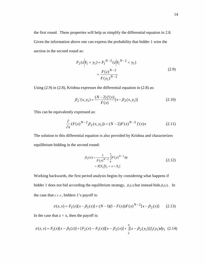
the first round. These properties will help us simplify the differential equation in 2.8.
Given the information above one can express the probability that bidder 1 wins the
auction in the second round as:
21
2
12
12
1112
)(
)(
)()(
N
N
NN
yF
zF
yYzFyYzF
(2.9)
Using (2.9) in (2.8), Krishna expresses the differential equation in (2.8) as:
)],([)(
)()2(),(' 1212 yxx
xF
xfNyx
(2.10)
This can be equivalently expressed as:
xxfxFNyxxFx
NN )()()2()),()(( 312
2 (2.11)
The solution to this differential equation is also provided by Krishna and characterizes
equilibrium bidding in the second round:
][
)()(
1)(
122
0
222
YxYYE
dyyFxF
xx
NN
(2.12)
Working backwards, the first period analysis begins by considering what happens if
bidder 1 does not bid according the equilibrium strategy, )(1 x but instead bids )(1 z . In
the case that xz , bidders 1’s payoff is:
)]([)())(1)(1()]()[(),( 22
11 xxxFxFNxxzFxz N (2.13)
In the case that z < x, then the payoff is:
x
zdyyfyxxxxFxFzxzFxz 1111221211 )()]([)]()][()([)]()[(),( (2.14)

15
For (2.7) we have the following first order condition:
)]([)()()1()(')()]()[(0 22
1111 xxxFzfNzzFzxzf N (2.15)
The first order condition for equation 2.7 is: )]()[()(')()]()[(0 211111 zxzfzzFzxzf (2.16)
In equilibrium it is optimal to bid )(1 x , so setting z = x in either first order condition gives:
)]()([)(
)()(' 12
1
11 xx
xF
xfx (2.17)
Krishna shows that, by invoking the boundary condition that 0)0(1 , one can
rearrange (2.11), expressing it as:
)()()]()([ 2111 xxfxxFdx
d (2.18)
which has the following solution:
][
)()()(
1)(
12
01121
xYYE
dyyfyxF
xx
(2.19)
These results are summarized as Krishna’s Proposition 15.12:
Suppose bidders have single-unit demand and two units are sold by means of sequential first-price auctions. Symmetric equilibrium strategies are
][)(
][)(
1222
121
YxYYEx
xYYEx
I
I
The two-unit sequential auction case can be generalized to a case where K units
2 Krishna (2002, pg. 214).
16
are sold in sequential, first-price auctions. By following essentially the same procedure
of maximizing expected payoffs, Krishna shows that the equilibrium bidding rule in any
period, k, is given by:
xkN
kkNk yFdyxF
x0
1 ))(()()(
1)( (2.20)
An explicit solution to (2.17) can be derived by working backwards and is expressed in a
generalization of proposition 15.1. Proposition 15.23 states:
Suppose bidders have single-unit demand and K units are sold by means of sequential first-price auctions. Symmetric equilibrium strategies are given by
][)( 1 kkI
k YxYEx
where )(xIk denotes the bidding strategy in the kth
auction and )1( Nkk YY is the kth highest of N-1
independently drawn values. Krishna shows that the same approach used earlier to derive an expression for the
equilibrium bidding strategy for a simple auction (what was referred to as the benchmark
model by McAfee and McMillan) can also be used to derive closed form representations
for optimal bidding strategies in a much more complicated auction.
These results concerning bidding strategies presented here are significant
because the game theoretic foundations of auction theory rely on attributing
characteristics of auctions, such as observed prices, to strategic behavior. Once we
3 From Krishna (2002, p.215)
17
derive a bidder’s best response function to an arbitrary strategy that he supposes his
rival(s) to be using, the Nash condition is exploited to yield each bidder’s equilibrium
bidding function. This traditional approach would suggest that our problem of modeling
the shrimp license buyback program is simply a problem of choosing the correct auction
model, obtaining an expression either analytically or numerically for optimal bidding
strategies, then applying one of the empirical techniques survey by Perrigne and Vuong
(1999) to back out a set of private valuations.
Learning in Sequential Auctions
The game theory-based models presented earlier largely ignore the component of
information transmission over time. We see this quite clearly in Krishna’s proposition
15.2 which states that equilibrium strategies for a given round of a sequential auction are
independent of realizations of price in previous bidding rounds. Although it seems quite
intuitive that bidder’s should use information from prior rounds when submitting bids in
a sequential auction, I could find very little in the auction literature attempting to
incorporate learning.
Jeitschko (1998) presents a model where bidders update a subjective probability
regarding the valuation type of their opponents in a sequential auction. His model is a
sealed bid, first-price auction with three players and two rounds. Each player can be one
of two types: a high type or a low type. A high type bidder has high value for the object
being auctioned and a low type bidder has a low value for the object. He also assumes
that players have unit demand. Learning is introduced in his model because each bidder
has a belief about the type of the other bidders. After observing the outcome of the first

18
auction, the remaining players revise their beliefs about their opponent’s type. Jeitschko
shows that the information generated by the sequential auction format has a positive
value to bidders. He contrasts the equilibrium strategies resulting from a model allowing
learning with the equilibrium implied by a myopic model and finds that bidders who are
allowed to react to information place lower bids, on average, and have higher payoffs.
This result is important for our study in that it suggests, quite strongly, that the true
model for sequential auction data should include information transmission over time.
Recently, the heavy reliance on strategic behavior to explain bidding has been
challenged in the experimental literature, most notably by Ginsberg (1998) and Deltas
and Kosmopoulou (2004). Among the most troubling results is Krishna’s derivation of
optimal bidding functions in sequential auctions, which show that the bids in any round
of the auction should be independent of prices in previous rounds. The trends in our data
clearly indicate the presence of a speculative component which seems to be due to the
dynamic nature of the problem. In the early rounds of the auction we observe very high
bids which seem to be distributed quite randomly. As the auction progresses we see bids
tending to cluster very tightly around the average buyback price. In the second round of
the auction there are a large number of very high bids but by the twelfth round bids are
clustered very tightly around what these license holders think the agency will accept.
These data suggest that there is a pronounced learning component in this auction and
some type of probability updating may help explain bidding behavior. Our challenge
then is to find a model flexible enough to allow us to analyze the speculative premium
19
induced by the sequential nature of the auction while retaining some consistency with
theory.
In Chapter IV I will contend that the problem of an individual license holder in
this auction can be visualized as a dynamic optimization problem where the fisherman
balances current expected payoff (which is reflected by the bid amount) and the
discounted future payoff from keeping the license for another period. This approach is
not entirely new. Oren and Rothkopf (1975) showed that dynamic programming can be
used to derive optimal bidding strategies when a bidder’s strategy in one auction affects
his rivals’ strategies in subsequent auctions.
The authors use the bidder’s strategy as the control in their model and use the
collective behavior of the bidder’s rivals as the state variable. The state equation in their
model represents the rival’s reaction to the bidder’s strategy. My model is similar in that
I am modeling the bidding problem as a dynamic, multistage process where the bid in a
given period is the control. However, I consider the state variables to be parameters of a
distribution reflecting the bidder’s subjective probability that a bid will be accepted. As
he places bids and observes the outcome (either agency accepts his bid or rejects it) he
revises this subjective probability. Our state equation is one which describes how the
parameters of the distribution change as the bidder receives information over time.
Summary
The economic literature has a long history of using a game-theory based approach
to derive the functions defining optimal bidding in an auction. While this approach has
been effective in addressing certain questions of traditional interest (for example, many
20
of the works cited in this chapter have as a principal objective the comparison of revenue
properties across different types of auctions), it seems to lack the flexibility to shed light
on our principal question of interest: does the sequential auction induce a speculative
premium.
Although the model I present in Chapter IV represents a departure from the main
approaches surveyed in this literature review, the importance of this chapter should not
be underestimated. In fact our departure from more traditional modeling methods
illustrates one important contribution of our work: namely, the estimation of a dynamic
optimization based model for optimal bidding in a sequential auction which does not rely
on the assumption of truthful revelation.

21
CHAPTER III
LESSONS FROM THE TEXAS INSHORE SHRIMP FISHERY
Introduction
The ability of buyback programs to successfully promote efficiency has been
questioned extensively in the economic literature (Larkin, Keithly, Adams, and
Kazmierczak 2004; Mullin 2001; Weninger and McConnell 2000). However, despite
economists’ concerns, buyback programs continue to find favor with fisheries managers
who often must balance biological, economic, and social goals.
In Chapter I I refer to 3 criteria which fishery managers must frequently consider
when making policy: biological conservation, economic efficiency, and welfare.
Because buyback programs may be designed to address all three of these goals, they have
traditionally found favor with fisheries managers. If buyback programs are able to
address biological, economic, and social goals within a single policy, then they will
likely continue to be implemented as budgets permit.
Given the past popularity and likely continued implementation of buybacks in
fisheries management, it is important to understand how these programs affect fisheries
and how individuals respond to the incentive structures created by them. In this chapter I
use the Texas Inshore Shrimp License Buyback Program as a backdrop for understanding
the effects of buybacks on demographics and fleet characteristics of the fishery, as well
as understanding how individuals behave under a buyback management regime.
I present data on fleet size and composition, bidder characteristics, and bidding
behavior in order to completely describe this program. Fleet statistics speak to the effect

22
that the program has had on the shrimp fleet in the Texas bays. Individual characteristics
shed light on the state of the bidders in the fishery and, finally, individual behaviors
illustrate how agents respond to the sequential auction format.
The goals for this chapter are two-fold. First, I aim to provide an understanding
of how buyback programs affect the nature of the fisheries they govern by presenting
trends in Texas Inshore Shrimp Fishery data. I also hope to provide a clear picture of
how individual agents respond to the incentive structure provided by sequential buyback
auctions in order to help fisheries managers understand the implications of this type of
program.
Literature
Our data analysis makes an important contribution to two existing bodies of
literature. The first is a general discussion on the role of buyback programs in fisheries
management and the second is a well-know sequential auction phenomenon, the
declining price anomaly. Here I discuss briefly how our study contributes to these two
areas of research.
The recent popularity of buyback schemes as a fisheries management tool has
produced a large and growing body of literature on the effects of buyback programs on
overcapitalized fisheries. Holland et al. (1999) provide an extensive review buyback
programs throughout the world. They present evidence from a number of programs in
order to make some general conclusions regarding the ability of buyback programs to
conserve stocks, rationalize the fleet and provide income redistribution. Grooves and
Squires (2007) follow up on this work and present a thorough overview of general
23
reasons for and consequences of buyback programs. Our study fits within this body of
literature by providing an in-depth account of the impact of a particular buyback type
(the sequential license buyback program) on the Texas inshore shrimp fishery.
The Declining Price Anomaly
The general subject of auctions is a well explored topic in the economic literature
with a variety of sub-topics. One of these subtopics is the declining price anomaly, a
phenomenon observed in many sequential auctions. Since the Texas Shrimp License
Buyback Program provides a set of data generated by a sequential auction, these
observations provide some empirical evidence relevant to the discussion of the declining
price anomaly.
This auction mechanism provides many opportunities for fishermen to behave
strategically. Each round of bidding gives participants new information about the
probability that a particular bid will be granted. The sequential nature of the auction
allows bidders to use information from previous rounds in forming bids for the next
round. The focus of the next chapter in this dissertation will be modeling how bidders
use this information.
It has been noted that, in sequential auctions, identical items tend to sell for less
in later rounds than in earlier ones. This phenomenon has been termed the “declining
price anomaly” and several empirical studies in the economic literature have confirmed
its existence (Ashenfelter 1989; McAfee and Vincent 1993; van den Berg, van Ours, and
Pradhan 2001). A clear and concise summary of relevant auction theory is provided by
van den Berg et. al (2001):

24
Somewhat loosely, one may state than an English auction is truth-revealing whereas a Dutch auction requires strategic behavior. The simple structure of the one-unit English auction vanishes if two identical objects are auctioned sequentially. Now, in the first round it is optimal for bidders to shade their bids to account for the option value of participating in the subsequent second round (Robert J. Weber, 1983). Bidders with a higher valuation also have a higher option value. Therefore, they shade their bids in the first round by a greater amount than do bidders with a lower valuation. As the auction proceeds, the number of bidders decreases. Over the sequence of auctions, the number of objects decreases as well. The first fact has a negative effect on the competition for an object and second has a positive effect. Both effects cancel out and prices follow a martingale. As a result, all gains to waiting are arbitraged away and the expected prices in both rounds are the same. The latter result also holds for sequential auctions of more than two objects and does not depend on whether the auction is English or Dutch. This neat theoretical result is not supported by empirical research, which usually finds price declines.
While our data includes bidders who are sellers not buyers, their behavior can
still be interpreted in the context of the declining bid anomaly. Bidders who are buyers
decrease their probability of success as they adjust their bids downwards and for bidders
who are selling it is the opposite. In examining the data from the buyback program, I
will show that participants tend to bid high (decreasing their probability of success early
on) in early rounds and, as the auction progresses and they learn about the agency’s
values, bids decline (increasing their probability of success later). This pattern runs
contrary to empirical evidence from traditional auctions which finds that buyers’ bids
tend to be high early on and decline as the auction progresses.

25
A Background on the Texas Shrimp License Buyback
Biology4
The lifecycle of the Gulf of Mexico panaeid (brown, pink, and white shrimp) is
approximately one year. Mature shrimp spawn in the gulf and their eggs are carried into
freshwater estuaries by the tides. Juvenile shrimp migrate from the estuaries into the
bays the, eventually, the offshore gulf where the cycle continues.
History
The shrimp fishery has traditionally been the largest and most valuable fishery in
the state. Prior to the license buyback program Texas had historically managed its
shrimp fishery through closures. This allowed shrimp to reach a larger size before
harvest and larger shrimp fetch high prices. However, between 1970 and the start of the
buyback program in 1995 there was a severe increase in effort in the Texas bays. This
effort increase led to a shortage of large shrimp for inshore as well as offshore gulf
shrimpers (Robinson, Cambell, and Butler 1994). To counteract the income effects of
harvesting smaller shrimp, fishermen resorted in increasing effort in an attempt to land
more total pounds.
The shrimp license buyback program, administered by the Texas Parks and
Wildlife Department (TPWD), was adopted in 1995 to address the sharp decline in
4 Biological information is taken from Texas Parks and Wildlife Department (2002). Readers interested in a more detailed discussion of the lifecycle for Gulf of Mexico shrimp should consult this report.

26
profitability of the shrimp fishing industry5. TPWD began retiring licenses in 1996.
Partial funding for the license buybacks was created through a $3 increase in the cost of
the saltwater fishing stamp. The overriding goal of this program was to reduce
overcapitalization without imposing severe economic damages on coastal communities
(TPWD 2002).
Licenses
In Texas, each shrimp boat can hold up to three licenses; a bay license, bait
license and gulf license. Only bay and bait licenses are eligible for buyback; gulf
licenses are not. Each of these three licenses confers on its owner a different set of
rights.
Bay and bait licenses allow the holder to shrimp only in the bays and estuaries
whereas a gulf license permits the holder to fish in the offshore areas. Additionally, a
federal permit is required to shrimp beyond 9 nautical miles out to 200 nautical miles. A
bait license allows its holder to fish major bays and bait bays year round but imposes a
200 pound bag limit. Additionally, from November 15th to August 15th at least half the
catch must be kept in live condition. A bay license allows its holder to fish major bays
during the spring open season, from May 15th to July 15th, and the fall open season, from
August 15th to November 30th. Bay license holders may also fish major bays south of the
Colorado River during the winter open season from February 1st to April 15th. There are
5 Funk, Griffin, Mjelde and Ward (2003) provide a good discussion of the legislation enacting the program and the funding structure.

27
no bag limits imposed during the winter or fall open seasons while the spring open
season has a 600 pound bag limit6.
Auction Rules
In order to understand the trends observed in this auction, it is important to
understand the basic rule structure of the program. The auction itself is a reverse
sequential auction with nonbinding bids. In the following discussion, I provide an
explanation of the auction mechanism.
The Texas Inshore Shrimp License Buyback Program purchases bay and bait
shrimp licenses via a sequential auction. At the start of each bidding round, license
holders may state a price at which they are willing to sell their license. TPWD then
scores these bids based primarily on the length of the vessel being bid on7. After scoring
the bids, TPWD makes formal offers to buy as many of the top scored bids as their
budget for that round allows. At that point, the license holder has an opportunity to
withdraw his or her bid and keep the licenses or sell the licenses for the bid price. For
this reason, we must distinguish between a bid that is accepted by TPWD and a bid that
is accepted by the fisherman. In the language of this program a bid is “granted” if it is
accepted by TPWD and a bid is said to be “accepted” if the offer from TPWD is accepted
by the fisherman. In order for a license to be bought back it must be granted and
accepted. Once a license is bought back, it is retired from the fishery.
6 For a complete description of the rights associated with each type of shrimp license see TPWD 2005. 7 We do not have the exact format that TPWD uses to score bids. Through personal communication with Robin Reichers we know that vessel length is the most important component of the bid score.

28
The Decision Making Environment
The introduction of the sequential buyback program created a rich decision
environment for shrimp license holders. In order to understand the many interesting
effects of this program on the fishery and fishermen’s interaction with it, it is important
to understand the choices available to bidders in the auction.
Beginning in 1996 license holders could decide to use or sell either of two
licenses. Licenses were also made transferable so, in addition to deciding whether to sell
a boat’s license back to TPWD or use it to fish, each owner had a third option: sell the
license to another fisherman. We can view each owner as managing a portfolio of assets
consisting of vessels and licenses, which define the rights of those vessels. In each round
of the auction the owner has the option of altering his or her portfolio by selling assets.
From Figure 3.1 one can see the options available to a single license holder in the
fishery. In each period a license holder must decide whether to try and sell the license in
that period. There are two possible markets for sales: the transfer market and the
buyback market. In the decision tree above, both of these decisions end in the owner
exiting the fishery. However, since the program retires only the licenses, sale of one
license does not preclude the fisherman from participating in other fisheries for which he
or she still owns a license or using the vessel in some other way. If a fisherman decides
not to attempt a sale, he or she can lease the license in that period or use it. These actions
end with the designation B. This is meant to convey that if the fisherman follows the Not
Sell portion of the decision tree he or she will end up in a state next period where all the
original options are available.

29
Figure 3.1. Single License Decision Tree
The decisions involved in holding a single license are complex, but few
fishermen in this fishery owned a single license at the start of this program. Most license
holders in our data set held both a bay and bait license. For shrimpers holding bay and
bait licenses on their boats the options available in each period expand greatly. Those
license holders owning both bay and bait licenses for a single boat can decide, not only
whether to sell a license, but also how many and which license(s) to sell..
To avoid over complication I don’t develop the possibility of adding a gulf
license to the asset mix, which adds further important complications. However, the
reader should realize that, in addition to a bay and bait license for a vessel, an owner may
hold a gulf license for that same vessel. In addition to the complexity added by the gulf
Bay or Bait(B)
Sell Not Sell
Transfer Mkt.
Buyback Mkt.
Lease Use
Exit Exit B B

30
license, some owners posses multiple vessels. This expands the number of possible
actions in the license holder’s portfolio management problem even further.
Re-entry
Once a license is purchased it is retired but, because licenses are transferable, it is
possible for a license holder to re-enter the fishery after selling a license. However, this
would require buying a license from a current license holder. So, while re-entry is
possible, the moratorium placed on new shrimp licenses in 1995 guarantees that in order
for someone to enter, or re-enter, the fishery someone else must exit.
This auction mechanism allows for a wide range of choices among bidders and
leaves open much potential for strategizing. In the sections that follow, one will explore
the bidding patterns observed under this sequential auction. First, one briefly discuss the
data relevant for this analysis.
Data
For this study I use data provided by TPWD. The data come from multiple
different files and, because there are some slight differences, it is important to explain
each.
First, the bidding rounds file contains a round-by-round record of every bid
submitted in the auction. This source reports the vessel and license being bid on, the
amount of the bid, whether TPWD granted the bid and, if the bid was granted, whether
the individual accepted that bid.
31
In order to incorporate demographic variables that may affect the license holder’s
bidding function I use the license holder database. This data set contains records for all
license holders in the fishery from 1997 – 2004. This file gives us vessel lengths, dates
of birth, and home ports for all license holders in the fishery. This demographic and
vessel characteristic data is important in helping us determine factors influencing bidding
behavior.
In many cases, auction data is only available for individuals who submitted
winning bids. An advantage of this data over traditional auction generated data sets is
that it contains information on all license holders, regardless of whether or not they chose
to bid. Therefore, in addition to observing factors affecting the size of a participant’s
bid, I also observe factors affecting the decision to place a bid.
At this point it is worth emphasizing that, while the first round of bidding was
carried out in 1996, the data only contain demographic information for license holders
beginning in 1997. So while I can report on auction statistics (number of licenses
purchased, amount spent, and average license price) for all 14 rounds, statistics such as
average length for vessels in the fleet or average age for all license holders can be
calculated only for rounds 2 – 14.
In addition to the auction and license holder data sets I also have data from
TPWD on vessel upgrades. Anytime a license holder alters a vessel it is recorded as a
vessel upgrade. The reader should understand that vessel upgrades include purchasing a
new boat or altering the length and/or horsepower of the current one. TPWD currently
has in place a restriction on the percentage by which fisherman can increase the length or

32
horsepower of their vessel. This restriction is in place to prevent capital stuffing8 or
effort creep that may occur with a buyback program.
Finally, I have economic data specific to the Texas bay system provided by
TPWD. This includes landings, ex-vessel values, and prices for shrimp from 1972 –
2002.
Licenses in the Fishery in 1997
The first year in which I have data for all license holders in the fishery is 1997. I
use this year as a baseline, from which changes are measured. Here I offer a picture of
the inshore shrimp fishery at the beginning of the buyback auction as a basis for future
comparisons.
At the start of our data in 1997 there were 2,948 shrimp licenses eligible for
buyback. Almost all of these licenses were held by individuals, not companies or
corporations. Of the licenses eligible for sale at the start, 817 individual fishermen and
1,792 unique vessels can be identified. Of the unique vessel owners in the fishery in
1997, 33% owned multiple boats and 67% were single vessel owners.
Among all licenses eligible for buyback, bay and bait licenses were almost
equally represented. There were 1,501 bay licenses and 1,447 bait licenses in the fishery
in 1997. The vast majority (96%) of vessels in the fleet held both bay and bait licenses
together.
8 Capital stuffing or effort creep is a well know phenomenon in regulated fisheries. The reader is referred to Townsend (1985) or, for a more specific discussion of capital stuffing in the Texas Inshore Shrimp Fishery, the reader may refer to Funk, Griffin, and Mjelde (2003).
33
Although they cannot be sold back, gulf licenses represent a potentially important
part of our data set. In 1997 about 30% of the vessel owners in the inshore fishery also
held a gulf license on at least one of their vessels. Moreover, about 10% of these owners
held a gulf license on the same vessel that was licensed to shrimp the bay system.
In sum, the Texas inshore shrimp fishery is comprised of a large number of small
owner/operators. The average vessel length for the fleet in 1997 was about 38 feet.
About one third of the fishermen owned multiple vessels and this same fraction held a
gulf shrimp license. In the next section I will look in detail at the auction’s effects on
this fishery.
Buyback Outcomes
In the previous section I presented a picture of the Texas inshore shrimp fishery
in 1997. In the discussion which follows I will examine the effect that the first 14 rounds
of the buyback auction had on this fishery. In particular I will provide a summary of
expenditures and key buyback results.
Scale of the Buyback Program
Perhaps one of the most distinguishing aspects of the Texas shrimp license
buyback program is its size. Table 3.1 shows a comparison of buyback programs in
recent U.S history9. Like many state run buyback programs it is small relative to
federally funded vessel buyback programs, but the Texas program is small even by state
9 The data in this table come from Muse (1999) as well as from our own data on the Texas inshore shrimp fishery provided by TPWD.

34
standards. From its start in 1996 to the 14th round in 2004 the Texas Inshore Shrimp
License Buyback Program spent $8.3 million, a modest sum in comparison to other
programs.
Table 3.1
Selected U.S Fisheries Buyback Programs
Fishery Date
Total Cost
(million $s) Type
BSAI Crab Fishery 2004 97.4 Vessel/License
Bering Sea Pollack Fishery 1998 90.2 Vessel/License
NE Groundfish 1995-1998 24.4 Vessel/License
WA Salmon Fishery 1995-1998 13.5 License
TX Inshore Shrimp Fishery 1996-2004 8.3 License
Although the Texas program operates on a financially smaller scale than most
U.S. buyback programs, the number of licenses sold through the buyback is quite large.
Table 3.2 shows the licenses retired in each round of the Texas program through the 14th
round. From the table below, one can see that TPWD typically buys back between 50 –
100 licenses per round. Furthermore, because the agency frequently holds more than one
bidding round per year, the total number of licenses bought out exceeded 100 in most
calendar years. In 1996 and 1997 the agency purchased only 30 and 37 permits
35
respectively. TPWD purchased at least 100 permits in every year from 1998 to 2004.
During that time, the fewest number of permits purchased in any year was 105 in 2000.
This was the fishery’s most financially successful year so it is not surprising to see
relatively few owners selling back10. The largest number of licenses purchased in any
single year was 219 in 2001. As a point of comparison, Washington State’s Salmon
License Buyback scheme retired 822 permits while the total number of licenses retired
by the Texas program is 1,207 and counting.
Licenses Retired
Through the 14th round of the Texas buyback 1,207 license had been retired.
Excluding the 30 licenses which were bought out in the first round, this leaves 1,177
licenses purchased between 1997 and 2004. This amounts to a 40% reduction in the
number of licenses over the relevant time period.
10 Personal communication with Michael Travis, Industry Economist, National Marine Fisheries Service, Southeast Regional Office.

36
Table 3.2
License Purchases by Round for the TX Program11
Round Year Licenses
Sold High Low
Avg. Purchase
Price Total Spent
1 1996 30 $6,000 $220 $3,394 $101,820 2 1997 41 $6,000 $100 $3,104 $127,227 3 1998 59 $6,400 $1,500 $3,692 $217,855 4 1998 53 $6,500 $2,500 $3,553 $188,345 5 1998 75 $7,000 $2,500 $4,632 $347,400 6 1999 116 $8,000 $2,500 $5,571 $646,250 7 2000 105 $8,600 $1,500 $6,273 $658,698 8 2001 77 $8,000 $2,500 $6,038 $465,000 9 2001 144 $8,500 $3,000 $6,255 $900,685 10 2002 122 $8,950 $3,000 $6,632 $809,185 11 2002 86 $9,500 $2,500 $6,998 $601,896 12 2003 117 $9,500 $2,300 $7,322 $856,694 13 2004 77 $9,000 $5,500 $7,464 $574,740 14 2004 105 $15,000 $4,360 $8,396 $881,670
Auction Totals 1,207 $7,431,465
Given this 40% reduction in the number of shrimp permits in the fishery, a
natural question to follow up with is, has this reduction led to measurable changes in the
inshore shrimp fishery? In this section I will examine changes in the biologic and
economic health of the fishery during limited entry.
11 A similar table appears in Reichers, Griffin, and Woodward (2007). Our table here includes rounds 13 and 14 of the auction.

37
Effort
Effort, measured in days fished12, dropped about 70% for the Texas inshore
shrimp fishery from 1995 - 200413. In addition, TPWD fly-over counts14 taken in 1995
and 2004 show a 67% decline in number of vessels on the water on opening day. In
1995, 886 vessels were counted on the water on opening day. By 2004 only 293 vessels
were counted on opening day. It should be noted that this decline is greater than the drop
in licenses attributable to the buyback program, suggesting that some fishermen may be
holding on to their license in order to sell it back, while using it less frequently.
CPUE
Catch per unit of effort (CPUE) is an important indicator of fleet efficiency.
From Figure 3.2 one see that CPUE in the Texas bay system stayed approximately
constant from 1995 to about 2002 and increased precipitously in 2003 and 2004. The
difference from 1995 to 2004 was about 233 pounds per unit effort, which amounts to an
increase of about 40% in CPUE. And during this time, total licenses in the fishery fell
by 34%.
12 One day fished is equal to 24 hours of continuous trawl time. 13 This figure is calculated from effort estimated by Griffin. Effort estimates from NMFS show a similar pattern of decline. 14 On August 15th (Opening day of the fall open season) TPWD performs aerial counts of actual number of vessels in each major bay. It should also be noted that the aerial counts performed on the first day of spring open season, May 15th, reveal a similar pattern.

38
0
100
200
300
400
500
600
1995 1996 1997 1998 1999 2000 2001 2002 2003 2004
Year
CP
UE
Figure 3.2. Catch per Unit Effort (CPUE) for the TX Inshore Shrimp Fishery 1995 -
2004
Landing and Ex-vessel Values
While the recent rise in CPUE suggests that the inshore shrimping fleet is
harvesting with greater efficiency, the trends in shrimp landing and ex-vessel values
paint a much gloomier picture. From data kept by TPWD for the Texas bay system I
calculate that, in 2004, landings for pink and brown shrimp from the Texas bays were
down 77% from the ten year average from 1985-1995. Additionally, ex-vessel values for
pink and brown shrimp were down 86% from the average of the ten year period
preceding limited entry. Table 3.3 provides an illustration of changes in key indicators
during limited entry.
39
Table 3.3
Key Indicators of the Health of the TX Inshore Shrimp Fishery
Ex-Vessel Value
Ex-Vessel Price Landings
Fly-Over Vessel Count CPUE
Baseline15 12,424.21 3.13 5,221.63 886 0.55
2004 5,336.20 3.03 3,307.80 293 0.80
% Change -57 -3 -37 -67 +45
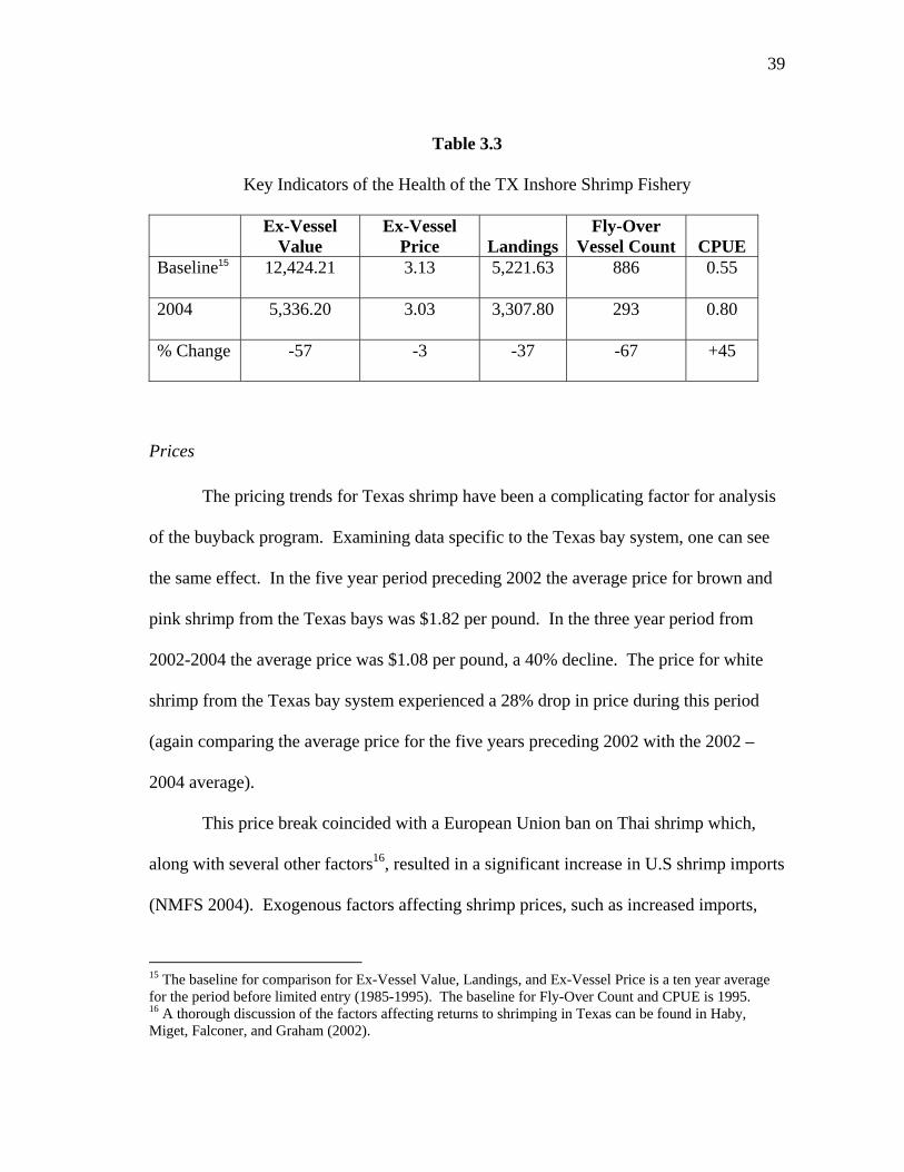
Prices
The pricing trends for Texas shrimp have been a complicating factor for analysis
of the buyback program. Examining data specific to the Texas bay system, one can see
the same effect. In the five year period preceding 2002 the average price for brown and
pink shrimp from the Texas bays was $1.82 per pound. In the three year period from
2002-2004 the average price was $1.08 per pound, a 40% decline. The price for white
shrimp from the Texas bay system experienced a 28% drop in price during this period
(again comparing the average price for the five years preceding 2002 with the 2002 –
2004 average).
This price break coincided with a European Union ban on Thai shrimp which,
along with several other factors16, resulted in a significant increase in U.S shrimp imports
(NMFS 2004). Exogenous factors affecting shrimp prices, such as increased imports,
15 The baseline for comparison for Ex-Vessel Value, Landings, and Ex-Vessel Price is a ten year average for the period before limited entry (1985-1995). The baseline for Fly-Over Count and CPUE is 1995. 16 A thorough discussion of the factors affecting returns to shrimping in Texas can be found in Haby, Miget, Falconer, and Graham (2002).

40
make it difficult to assess the buyback programs’ effects on the economics of the inshore
shrimp fishery in Texas.
Capital Stuffing
A major critique of buyback programs is that they will tend to induce capital
stuffing. By removing effort from the fishery and pushing up the output price, those
owners who stay in will have an incentive to expand their operations. Considering the
economic state of the fishery discussed previously it is probably not surprising that there
is little evidence to suggest that capital stuffing has been a problem.
In addition to license holder demographics and bidding behavior, I have data on
the number of vessel upgrades. Through 2004, TPWD processed 250 vessel upgrades.
Among these, 149 were upgrades to a larger vessel and, while boat length is not a perfect
indicator for capacity, this is the best proxy currently available. The 149 vessel upgrades
that involved a size increase account for roughly 8% of the vessels in the fleet in 1997.
The average size increase of these upgrades was 3.6 feet. So, while we do see a small
percentage of owners expanding operations, the overall incidence of capital stuffing
appears small, which comes as no great surprise considering the economic conditions
prevailing in the fishery.
Outcome summary
The statistics presented in this section are meant to illustrate the state of the Texas
inshore shrimp fishery. I have provided statistics on key economic and biological
indicators in order to try and measure the program’s impact on the fishery. Among the

41
many trends presented here one stands out as particularly salient: real effort17 has
declined substantially since the imposition of limited entry.
However, because of the price shock realized in 2002, it is very difficult to
attribute effort reductions solely to the buyback program. At most it can be concluded
that the program is adding another incentive to what was already a very strong case for
exiting this fishery. However, since intervention in fisheries typically arises in order to
address an already bleak situation, the same can easily be said for fleet rationalization in
general. In the sections that follow I will move away from the macro discussion and
focus on several interesting micro issues. I will analyze the buyback program’s effects
on age composition in the fishery, vessel characteristics, and explore individual behavior
in the auction itself.
Auction Behavior
In this section I will take an informal look at some important factors influencing
bidding behavior in the sequential auction. Unfortunately, practical considerations
prevent us from incorporating all of these into the formal econometric structure of
Chapter IV. Hence, these observations provide strong motivation for extensions to our
econometric model.
Because much of the money used to finance the Texas program is generated by
the state in the form of fees on recreational and commercial fishermen, the funds
17 As noted in Griffin, Shah, and Nance (1997), “A unit of nominal effort is defined as net(s) being pulled in the water for a period of 24 hours (known in the industry as a day fished). Standardized effort is defined as adjusted nominal effort based on the relative fishing power (RFP) of each vessel in the Gulf of Mexico shrimp fleet relative to a standard vessel.”
42
available in any given year are small. Due to these financial constraints the program is
run as a sequential auction. In each round the agency uses its budget to buy back as
much capacity as they can afford and, when more money becomes available, they hold
another round. This sequential format leads to behavioral complexities and interesting
dynamic pricing patterns. In the sections that follow I will explore some of the factors
influencing observed behavior in the auction and outcomes associated with the repeated
game set-up.
Age/Length Effects
In this section I examine the interaction between two key proxy variables and the
buyback program. I use vessel length as a proxy for effort and license-holder age serves
as a proxy for experience. Here I present the effects of the buyback on average age and
vessel length in the inshore shrimping fleet as well as patterns in auction bidding across
different age and vessel size classes.
Although it is difficult to determine what effect the buyback program has had on
productivity in this fishery, its impact on the characteristics of the fishery are clear. Two
effects on fleet composition which stand out are the program’s effect on average age of
the license holders in the fishery and average vessel size in the inshore shrimp fleet. This
buyback auction has demonstrated a propensity to buyout older license holders and
smaller vessels.
First I look at the age of those shrimpers choosing to exit the fishery by selling
back licenses. These figures show that older license holders are tending to sell out of this
fishery faster than young ones. At the start of this buyback program, the average age of

43
all license holders in the fishery was 47. By round 14 this average had increased by only
2 years to 49. Calculating the average age for fishermen who sold their licenses in each
round, we find that the mean age of sellers exceeds the mean age of all license holders in
every round. Apparently older fishermen are more likely to get out of the fishery—not
surprising—but they also find the buyback program to be more attractive than the
transfer market. Given the tendency of the buyback to remove older license holder from
the fishery, it is very possible that many participants are using the buyback to generate
some savings for retirement. These results are illustrated in Figure A.1 in Appendix A.
Next, I examine changes in vessel length for the inshore fleet. I find that the
average length of vessels in the inshore fleet has increased steadily as the auction has
progressed. This is due in part to the propensity of the TPWD to grant bids for smaller
boats.
In all but 4 of the 14 rounds at least 70% of the buyout offers were made to boats
smaller than the median vessel length for the entire fleet in that round. Likewise, in 7 of
the 14 rounds over half of the buyout offers were made to boats in the first quartile of the
age-vessel length distribution. The result has been a 5% increase in the average vessel
length of the fleet since 1995. Figure A.2 in Appendix A shows the trend in average
vessel length for the fleet over time. Without a counterfactual scenario it is impossible to
tell whether such a trend would have occurred in the absence of the buyback program.
However, by purchasing the smaller vessels, it is safe to say that the program has
exacerbated this trend.

44
The question that arises naturally then is, “are the trends in age of the owners and
the length of the vessels two separate trends or a single one?” This question can be
answered somewhat informally by examining the age/vessel length distribution for the
fishery.
At first glance, vessel lengths seem to be distributed fairly evenly across age
classes. In 1997, 56% of vessels below the median length were owned by fisherman
above the median age. So about half of the small vessels are owned by old fishermen
and about half are owned by young fishermen. Among vessels above the median length,
45% were owned by fishermen above the median age. The average vessel length for all
license holders above the median age in 1997 was 37.2 while the average vessel length
for license holders below the median age was 40.3. From these figures it does not appear
that older fishermen necessarily own smaller boats. In fact, the correlation between age
and vessel length for all bidders is very weak (-0.094). However, as shown in Figure 3.3,
younger fishermen owned a disproportionate number of the largest vessels. At the start
of the program, among vessels in the fourth quartile of the distribution (from 45 – 94 ft),
60% were owned by fishermen below the median age. Among the largest 10% of boats
in the fishery in 1997 (those 50 ft or greater), only 35% were owned by license holders
above the median age. So, while most of the vessels in the fishery are distributed fairly
evenly among age classes, the largest vessels belong almost exclusively to young
fishermen.

45
0
50
100
150
200
250
Vessels
14-31 ft 32-37 ft 38-43 ft 44-72 ft
Old Fishermen
Young Fishermen
Length Classes
Old Fishermen
Young Fishermen
Figure 3.3. Vessel Length Distribution by Age of Owner in 199618
Effects on Bidding
In Chapter IV I will develop a formal dynamic econometric model to estimate
parameters of the bidding function that will allow us to identify variables affecting the
underlying value of the licenses. In particular, I suspect that vessel length, shrimp price,
and license holder age will influence the size of the bid submitted to the auction. In this
section I propose a simple model to test the hypothesis that these three independent
variables help explain bids.
Here I propose a Heckman two-stage estimation model as a first attempt at
modeling the fisherman’s bidding function. A two-stage model is appropriate in this
case because I suspect that there may be significant differences in the underlying license
18 Here we use two age classes and four length classes. The age classes are defined as fishermen above the median age for all license holders (old fishermen) and those below (young fishermen). The length classes are separated by quartiles of the distribution of lengths for all vessels in the fishery in 1997.

46
valuation between those owners who chose to participate in the auction and those who do
not. In this auction average bid per foot of boat length19 is higher for bidders older than
the median age. However, we also observe that the average age of all fishermen who
submit bids is higher than the average age for all license holders. This suggests that
there may be a sample selection bias. To solve the problem of discerning the effects of
our suspected drivers on bidding while also accounting for their effects on the
participation decision I first estimate the following Probit model for the participation
decision:
)()1( 43210 GULFOWNPLENGTHAGEGxBidYNP 20
In the equation above BidYN is a binary variable indicating whether a fisherman
submitted a bid for that license or not. AGE, LENGTH, and P are continuous
independent variables indicating the age of the license holder, length of the vessel to
which the license is attached, and shrimp price respectively. GULFOWN is a binary
variable indicating whether the vessel is also licensed to shrimp in offshore areas. The
function G() is the cumulative density function of the standard normal distribution.
Our sample includes observations of several thousand licenses over 14 time
periods (rounds). There are a total of 38,671 observations in our sample, in 2,676 of
these the dependent variable takes a value equal to 1. The results of the Probit regression
are shown in Table 3.4 below.
19 Here we are talking about all bids placed, which does not necessarily mean they were granted. 20 Here we use the notation of Woolridge 2003.
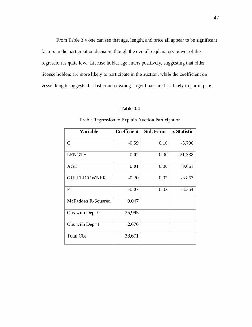
47
From Table 3.4 one can see that age, length, and price all appear to be significant
factors in the participation decision, though the overall explanatory power of the
regression is quite low. License holder age enters positively, suggesting that older
license holders are more likely to participate in the auction, while the coefficient on
vessel length suggests that fishermen owning larger boats are less likely to participate.
Table 3.4
Probit Regression to Explain Auction Participation
Variable Coefficient Std. Error z-Statistic
C -0.59 0.10 -5.796
LENGTH -0.02 0.00 -21.338
AGE 0.01 0.00 9.061
GULFLICOWNER -0.20 0.02 -8.867
P1 -0.07 0.02 -3.264
McFadden R-Squared 0.047
Obs with Dep=0 35,995
Obs with Dep=1 2,676
Total Obs 38,671
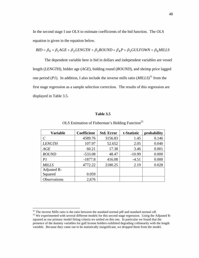
48
In the second stage I use OLS to estimate coefficients of the bid function. The OLS
equation is given in the equation below.
MILLSGULFOWNPROUNDLENGTHAGEBID 6543210
The dependent variable here is bid in dollars and independent variables are vessel
length (LENGTH), bidder age (AGE), bidding round (ROUND), and shrimp price lagged
one period (P1). In addition, I also include the inverse mills ratio (MILLS)21 from the
first stage regression as a sample selection correction. The results of this regression are
displayed in Table 3.5.
Table 3.5
OLS Estimation of Fisherman’s Bidding Function22
Variable Coefficient Std. Error t-Statistic probability C 4589.76 3156.83 1.45 0.146LENGTH 107.97 52.652 2.05 0.040AGE 60.21 17.38 3.46 0.001ROUND -533.08 48.47 -10.99 0.000P1 -1877.8 416.08 -4.51 0.000
MILLS 4772.22 2180.25 2.19 0.028Adjusted R-Squared 0.059
Observations 2,676
21 The inverse Mills ratio is the ratio between the standard normal pdf and standard normal cdf. 22 We experimented with several different models for this second stage regression. Using the Adjusted R-squared as our primary model fitting criteria we settled on this one. In particular we found that the presence of the dummy variables for gulf license holders exhibited degrading collinearity with the length variable. Because they came out to be statistically insignificant, we dropped them from the model.
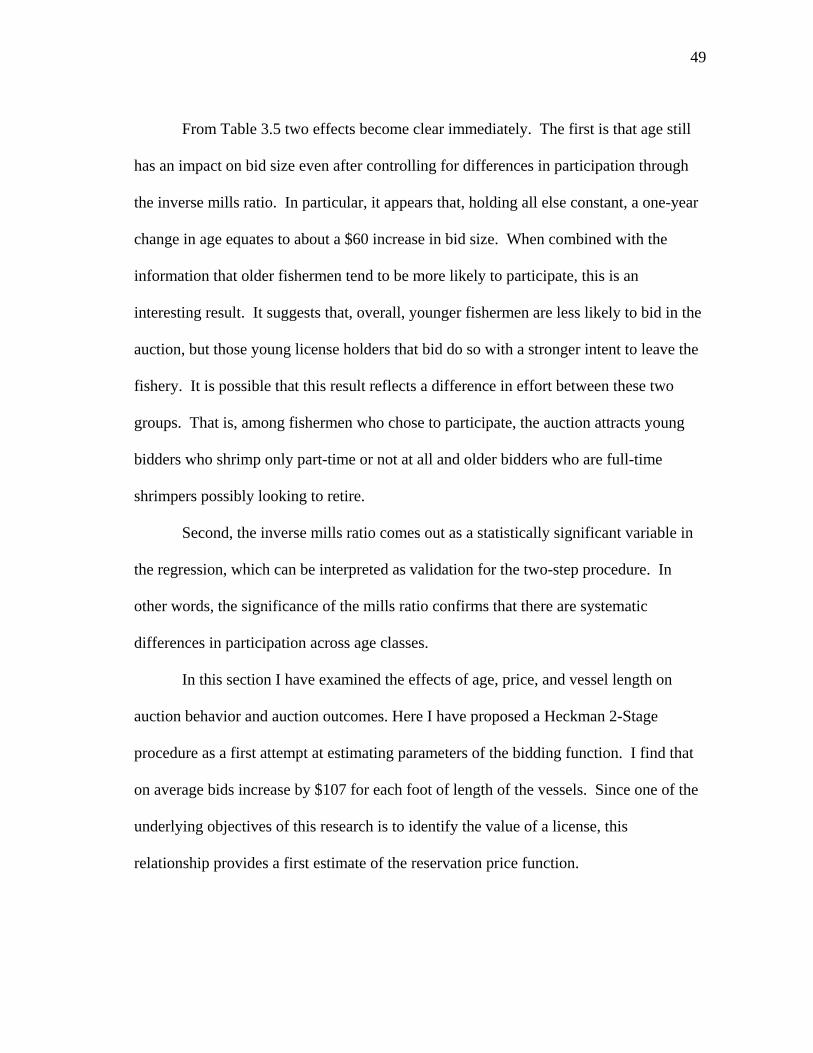
49
From Table 3.5 two effects become clear immediately. The first is that age still
has an impact on bid size even after controlling for differences in participation through
the inverse mills ratio. In particular, it appears that, holding all else constant, a one-year
change in age equates to about a $60 increase in bid size. When combined with the
information that older fishermen tend to be more likely to participate, this is an
interesting result. It suggests that, overall, younger fishermen are less likely to bid in the
auction, but those young license holders that bid do so with a stronger intent to leave the
fishery. It is possible that this result reflects a difference in effort between these two
groups. That is, among fishermen who chose to participate, the auction attracts young
bidders who shrimp only part-time or not at all and older bidders who are full-time
shrimpers possibly looking to retire.
Second, the inverse mills ratio comes out as a statistically significant variable in
the regression, which can be interpreted as validation for the two-step procedure. In
other words, the significance of the mills ratio confirms that there are systematic
differences in participation across age classes.
In this section I have examined the effects of age, price, and vessel length on
auction behavior and auction outcomes. Here I have proposed a Heckman 2-Stage
procedure as a first attempt at estimating parameters of the bidding function. I find that
on average bids increase by $107 for each foot of length of the vessels. Since one of the
underlying objectives of this research is to identify the value of a license, this
relationship provides a first estimate of the reservation price function.

50
There are, however, some limitations to this approach. First, I find that on
average, and controlling for length and age of owner, bids are declining from round to
round. This immediately calls into question the ability to infer from the bids evidence
about the reservation price of the vessels. Economic intuition would suggest that lower
valued bids would tend to be bought out earlier so that the average value of licenses in
the fishery would rise over time. Since the results from the second-stage regression runs
exactly counter to this result, it calls into question the ability to infer directly from the
bids evidence about the underlying value of licenses. Secondly, I find that, even after a
sample selection correction, the model had very little explanatory power.
In Chapter IV I provide an alternative to this static estimation that is capable of
capturing the dynamic elements of the bidder’s decision process. In particular, the
sequential auction allows bidders the opportunity to gather information about the
agency’s willingness to pay for a license. This informational effect is largely ignored in
the model presented here. The OLS estimation used here implicitly assumes a 1:1
relationship between the bid and the fisherman’s reservation price. In the next chapter I
propose an econometric model which relaxes this assumption by incorporating the
fisherman’s subjective expected probability of success in the auction. The 2-Step
estimation procedure carried out here suggests that license holder age, shrimp price, and
vessel length are important elements of the bid function. In Chapter IV I will attempt to
incorporate these factors into a dynamic econometric model which will also be capable
of capturing the learning that goes on in a sequential auction. In the next section I take an
initial look at how bidding behavior has changed over time.
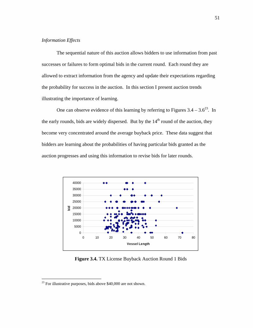
51
Information Effects
The sequential nature of this auction allows bidders to use information from past
successes or failures to form optimal bids in the current round. Each round they are
allowed to extract information from the agency and update their expectations regarding
the probability for success in the auction. In this section I present auction trends
illustrating the importance of learning.
One can observe evidence of this learning by referring to Figures 3.4 – 3.623. In
the early rounds, bids are widely dispersed. But by the 14th round of the auction, they
become very concentrated around the average buyback price. These data suggest that
bidders are learning about the probabilities of having particular bids granted as the
auction progresses and using this information to revise bids for later rounds.
0
5000
10000
15000
20000
25000
30000
35000
40000
0 10 20 30 40 50 60 70 80
Vessel Length
bid
Figure 3.4. TX License Buyback Auction Round 1 Bids
23 For illustrative purposes, bids above $40,000 are not shown.
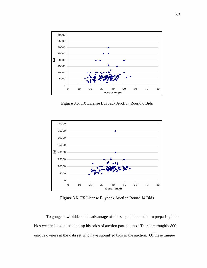
52
0
5000
10000
15000
20000
25000
30000
35000
40000
0 10 20 30 40 50 60 70 80
vessel length
bid
Figure 3.5. TX License Buyback Auction Round 6 Bids
0
5000
10000
15000
20000
25000
30000
35000
40000
0 10 20 30 40 50 60 70 80
vessel length
bid
Figure 3.6. TX License Buyback Auction Round 14 Bids
To gauge how bidders take advantage of this sequential auction in preparing their
bids we can look at the bidding histories of auction participants. There are roughly 800
unique owners in the data set who have submitted bids in the auction. Of these unique

53
owners, 406 have submitted bids in multiple rounds. That is, about half of all bidders in
the auction have participated in multiple rounds.
Our data on whether bids were granted or not tells an interesting story that is
consistent with the idea that the sequential auction may induce a speculative motive. Of
the almost 1,700 unique licenses in the auction, 796 have been bid on unsuccessfully (not
granted) at least once. In percentage terms this means that around 47% of all the assets
offered for sale in this auction were offered at a price greater than that which the agency
was willing to pay. Among the 1,177 licenses that were sold from round 2 through the
14th round, 363 of these had a prior bid rejected by TPWD before selling. This means
that roughly one out of every three licenses surrendered through the buyback auction was
bid on in a round prior to that in which it was ultimately sold.
I find that most bidders who sell a license after repeated bidding use a strategy of
bidding high early and lowering their bids monotonically in subsequent rounds, zeroing
in on their sell-out price from above. Two-thirds of the repeat bid licenses have been
sold using this approach.
The No Sale Option
A unique feature of this auction is that it offers fishermen an opportunity to
withdraw their bids after observing whether the bid was granted. Once the agency
decides to grant a bid they inform the license holder and, at this time, the fisherman can
decide to either execute the sale of the license or withdraw the bid. If the bid is
withdrawn, the license holder can continue fishing and possibly participate in the auction
again later. About 6% of the licenses that have been bid on through round 14 have

54
rejected an offer from TPWD at least once. Most of these licenses remained in the
fishery as of the 14th round of the auction but 32 of them had been sold. Seven of these
were sold for less than the originally rejected offer. Of the ones which collected positive
returns, the average return on exercising the no-sale option was about $1,700.24
Although it may sound irrational to sell a license for less then a higher bid which
was granted earlier in the auction, there is a plausible explanation for this behavior which
hinges on risk aversion: consider a fisherman who is experiencing a good return on his
license and is not strongly considering leaving the fishery. The fisherman decides to
submit a bid of $6,000 just to see if the agency will take it. The agency does but on
further reflection the fisherman decides to keep the license. Two years later returns have
become quite poor for the fisherman and he is desperate to sell back his license. He
knows that the agency was once willing to pay $6,000 for his license, but also knows that
the price the agency pays depends on all other bidders in the market and, therefore,
reasonably fears that a bid of $6,000 may not be granted. This plausible situation might
lead a fisherman to actually reduce his bids below a price that was previously accepted.
As stated earlier, these fishermen selling for a price below one that was previously
granted are anomalies. Most bidders who sell after rejecting an offer from the agency do
so at a price higher than that which was previously granted. If such withdrawals were
common the agency would be spending much more to buy out the same number of
licenses than would be retired if all bids were binding. And this is a concern since the
24 Return was calculated as the difference between the bid that was granted then rejected and the bid that was ultimately granted then accepted. These figures are net of license cost.
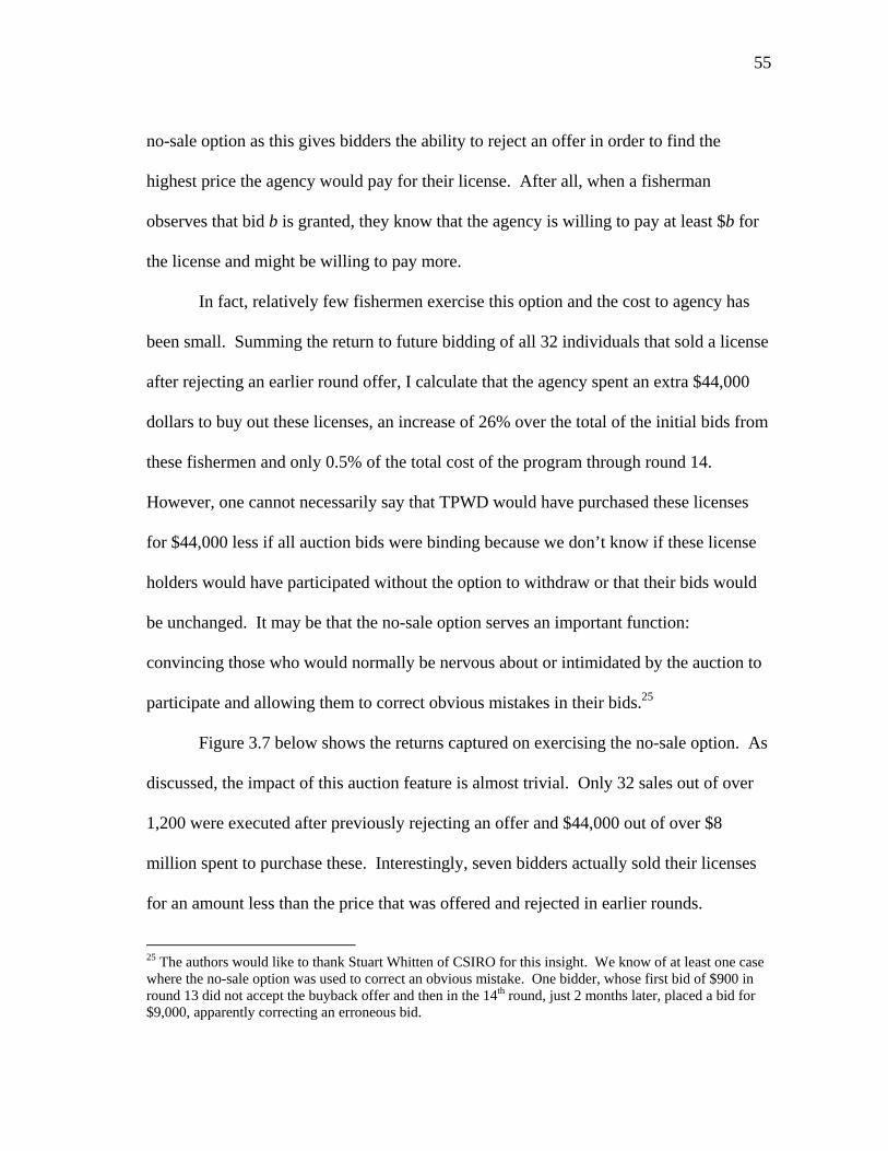
55
no-sale option as this gives bidders the ability to reject an offer in order to find the
highest price the agency would pay for their license. After all, when a fisherman
observes that bid b is granted, they know that the agency is willing to pay at least $b for
the license and might be willing to pay more.
In fact, relatively few fishermen exercise this option and the cost to agency has
been small. Summing the return to future bidding of all 32 individuals that sold a license
after rejecting an earlier round offer, I calculate that the agency spent an extra $44,000
dollars to buy out these licenses, an increase of 26% over the total of the initial bids from
these fishermen and only 0.5% of the total cost of the program through round 14.
However, one cannot necessarily say that TPWD would have purchased these licenses
for $44,000 less if all auction bids were binding because we don’t know if these license
holders would have participated without the option to withdraw or that their bids would
be unchanged. It may be that the no-sale option serves an important function:
convincing those who would normally be nervous about or intimidated by the auction to
participate and allowing them to correct obvious mistakes in their bids.25
Figure 3.7 below shows the returns captured on exercising the no-sale option. As
discussed, the impact of this auction feature is almost trivial. Only 32 sales out of over
1,200 were executed after previously rejecting an offer and $44,000 out of over $8
million spent to purchase these. Interestingly, seven bidders actually sold their licenses
for an amount less than the price that was offered and rejected in earlier rounds.
25 The authors would like to thank Stuart Whitten of CSIRO for this insight. We know of at least one case where the no-sale option was used to correct an obvious mistake. One bidder, whose first bid of $900 in round 13 did not accept the buyback offer and then in the 14th round, just 2 months later, placed a bid for $9,000, apparently correcting an erroneous bid.
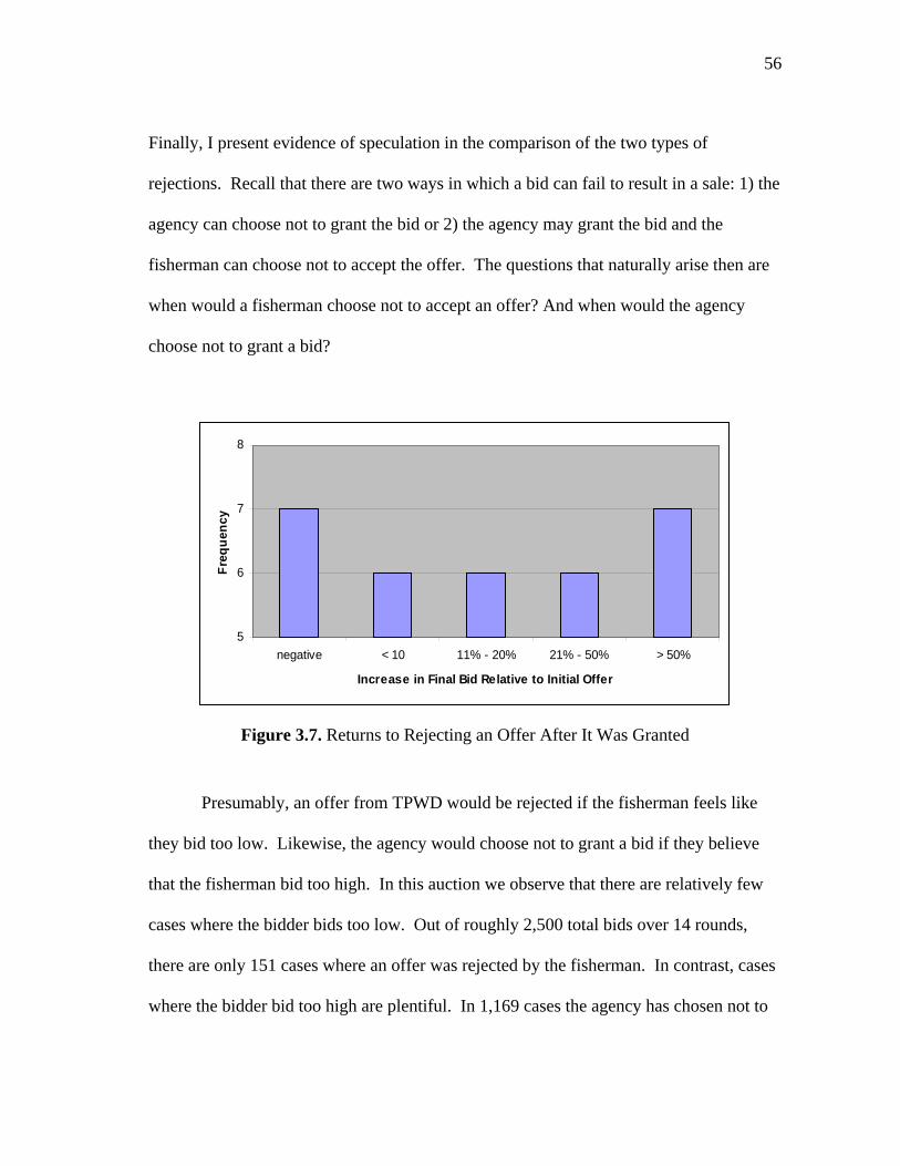
56
Finally, I present evidence of speculation in the comparison of the two types of
rejections. Recall that there are two ways in which a bid can fail to result in a sale: 1) the
agency can choose not to grant the bid or 2) the agency may grant the bid and the
fisherman can choose not to accept the offer. The questions that naturally arise then are
when would a fisherman choose not to accept an offer? And when would the agency
choose not to grant a bid?
5
6
7
8
negative < 10 11% - 20% 21% - 50% > 50%
Increase in Final Bid Relative to Initial Offer
Fre
qu
ency
Figure 3.7. Returns to Rejecting an Offer After It Was Granted
Presumably, an offer from TPWD would be rejected if the fisherman feels like
they bid too low. Likewise, the agency would choose not to grant a bid if they believe
that the fisherman bid too high. In this auction we observe that there are relatively few
cases where the bidder bids too low. Out of roughly 2,500 total bids over 14 rounds,
there are only 151 cases where an offer was rejected by the fisherman. In contrast, cases
where the bidder bid too high are plentiful. In 1,169 cases the agency has chosen not to
57
grant the bid. This means that the TPWD has deemed almost half of all bids to be too
high.
Information Effects Summary
In this section I have presented statistics related to the sequential nature of the
buyback auction in order to illustrate the importance of learning. Three results in
particular paint an especially clear picture of the role of information in this auction.
First, I have shown that bids as a function of vessel length are becoming tightly
condensed over time. Next, about half of all auction participants have submitted bids in
multiple rounds. And finally, I have shown that, among bidders who have bid in
multiple rounds, most do so because they bid too high not too low. Taken together these
three findings suggest that there is probably an element of speculation at play in this
auction.
Summary of Lessons from the TX Shrimp License Buyback
In this chapter I have presented trends from the Texas Inshore Shrimp License
Buyback Program as a means for further understanding sequential buyback programs.
Using license holder data on the inshore shrimp fleet over the first 7 years of the
buyback, I find an increase in the average length for vessels in the fleet and a noticeable
propensity for older license holders to sell out. In examining how individual agents
respond to the auction mechanism I find that a large portion of auction participants bid in
multiple rounds, suggesting that learning may play a role in the bidding process.
58
While it is difficult to make causal statements without first trying to establish a
counterfactual scenario, a few policy relevant observations can be made on the basis of
this analysis. First, there is evidence that the sequential auction framework has tended to
induce speculation among its participants, probably inflating bids. This result could have
important implications for managers hoping to get the most “bang for their buck” from a
buyback scheme.
I have also shown that systematic differences exist in both auction participation
rates and bidding behavior across age classes. For managers concerned with social
implications of buyback programs, this result will also be important. In particular, I
showed that older license holders were more likely to participate in the auction and were
exiting the fishery through the buyback program faster than young ones. This result may
be seen as favorable or unfavorable depending on where the agency falls with respect to
the three goals of buyback programs quoted from Holland et al. (1999) in the
introduction. If the buyback program is seen as a vehicle for providing transfer
payments to the industry then it may perfectly acceptable to buyout older license holders
faster as it could signal that the money is going to the “most deserving.” However, if the
overriding goal of the program is remove the most effort for the least money then the
propensity to buyout older license holder may be a concern as it suggests the agency is
buying out fishermen that were likely to retire anyway.
Finally, I have presented in this chapter an elementary econometric model of the
fisherman’s bid function. While parameter estimates from this model suggest that vessel
length, shrimp price, and license holder age are important drivers of bids submitted to the
59
auction, the counterintuitive coefficient on the round parameter and the low explanatory
power of the model suggests that something is missing. The Heckman procedure
presented in this chapter is not capable of capturing the learning that is made possible
when the same fisherman is allowed to bid on the same asset in multiple rounds of the
auction. In particular, I suspect that in any particular round of the auction a fisherman’s
bid will be based not only on factors affecting the underlying value of the license (vessel
length and shrimp price for example), but also on the fisherman’s perceived probability
of success for any particular bid. In the next chapter I will present an econometric model
capable of estimating the primitive variables of the fishermen’s reservations price
function by incorporating into the estimation the fact that bidding decisions take into
account the sequential auction and over time bidders learn more and more about the
probabilities of success for particular bids.

60
CHAPTER IV
AN EMPIRICAL MODEL OF BIDDING IN SEQUENTIAL AUCTIONS
Introduction
In 1995 the Texas State Legislature granted authority to the Texas Parks Wildlife
Department (TPWD) to begin purchasing inshore (bay and bait) shrimp licenses from
permit holders. In doing so they created a rich and complex decision making
environment for inshore shrimpers. In this chapter I present a dynamic econometric
model capable of describing the fisherman’s decision making process inside this
environment and use the model to estimate the effects of key variables, such as vessel
length and shrimp price, on the bidding function.
The sequential auction format used by TPWD offers participants the opportunity
to engage in strategic bidding for the purpose of gaining information about the agency’s
willingness to pay for a license. Therefore, I model the bidding decision as a dynamic
optimization problem. In order to estimate effects of key variables on the bidding
function I nest this dynamic optimization algorithm inside of a hill-climbing routine,
which will locate likelihood maximizing parameter estimates for the model.
The remainder of this chapter is organized as follows: The next section will
review the auction rules as motivation for our approach26. The following section will
discuss the contributions of this chapter in the context of two distinct bodies of literature.
I then present the empirical model and apply it to data collected from the auction from
26 Readers interested in a full discussion of the institutional setting should refer back to Chapter III.

61
1997 to 2004 and present the results of our estimation. Finally, I offer some
interpretation of these results and conclusions.
Motivation
The Texas Inshore Shrimp License Buyback Program purchases bay and bait
shrimp permits via a sequential, first price auction. At the start of each bidding round
license holders may state a price at which they are willing to sell their license. TPWD
then scores these bids27 and makes formal offers to buy as many of the top scored bids as
their budget for that round allows. At that point the license holder has an opportunity to
withdraw his or her bid and keep the permit or sell the permit for the bid price. For this
reason one must distinguish between a bid that is accepted by TPWD and a bid that is
accepted by the fisherman. In the language of this program a bid is “granted” if it is
accepted by TPWD and a bid is said to be “accepted” if the offer from TPWD is accepted
by the fisherman. In order for a license to be bought back it must be granted and
accepted. Once a license is bought back it is retired from the fishery.
Literature Relevant to the Estimation of Dynamic Decision Processes
This chapter makes a contribution to the literature on estimation of dynamic
models. More specifically, our estimation procedure is an important methodological
contribution to the literature on dynamic decision processes.
27 Bids are scored based on the length of the vessel being bid on, under the assumption that catch is positively correlated with length.
62
Dynamic Decision Processes
The starting point for our estimation procedure is the seminal 1987 paper by John
Rust. Rust (1987) developed the nested fixed point algorithm allowing the estimation of
parameters of an optimal stopping problem and in Rust (1988) he provided a guide to
maximum likelihood estimation of dynamic optimization problems. Also, in his chapter
in The Handbook of Econometrics (1994), Rust lays out quite clearly the details of and
assumptions necessary for maximum likelihood estimation of dynamic decision
processes. Prior to Rust’s paper, estimation approaches for dynamic decision problems
required highly restrictive functional form assumptions that would not be suitable in the
current setting.
Some other helpful applications and discussions of the estimation techniques for
dynamic decision processes have come from Miranda and Schnitkey (1995), Provencher
and Bishop (1997) and Schjerning (2005). Our problem contains two notable differences
from those previously considered. First, work in this area has traditionally focused on
problems containing a binary control variable while our key “control” variable, the bid
made by fishermen, is continuous over a range. Second, I consider “state” variables
which include the parameters of a subjective probability distribution and allow them to
evolve following a Bayesian updating process as the fishermen get information from
auction outcomes. Thus our state transition is notably more complex than those models
previously considered.

63
Model
Here I am proposing a model capable of estimating the magnitude of speculation
present in a sequential auction. The approach can be summarized as follows. The
function R( ) captures the benefit, to the fisherman, of holding a license in the current
period. This function captures the financial returns on holding a license as well as the
fisherman’s preferences for holding a license. By estimating parameters of this function
it is possible to identify differences in observed bids and the benefit function. I label this
difference the speculative premium. In this section I present in detail the empirical
model by which I will estimate the parameters of the function R.
Data Generating Process
Because observed bids come from a sequential auction I use a dynamic
framework as the basis to describe the data generating process. I assume that the bids
from the auction are the result of license holders solving a dynamic optimization
problem. In this section I will present the details of this optimization problem.
At the beginning of each round a fisherman chooses a bid,b . If the bid is granted
by the TPWD then the fisherman must choose whether to accept the agency’s offer. A is
a binary variable defined as:
sale executesbidder if1
offer rejectsbidder if0A
64
If the bid is not granted or is rejected28, the fisherman uses the license to fish in the
current period and collects returns equals to R , a function to be estimated. Define R as a
function of vessel characteristics, which are contained in the vector of state
variables, ,tx a parameter vector , and an error term . It is worth noting that ),;( txR
includes the economic returns to fishing but is sufficiently general to include individual
specific preferences and opportunity costs as well.
A fisherman who does not sell his license in the current period collects benefits
equal to R in that period but also has the opportunity to participate in the auction again
next period. Denote by );( 11 tt xV the value of arriving in the next period in state
.vector parameter with 1 tx The state vector 1tx captures vessel characteristics and
the fisherman’s expectation as to whether a bid will be accepted. Hence, for the
fisherman who does not sell his or her license in the current period, the discounted
present value of the stream of expected net benefits is ,1 tVR where is the discount
factor.
Since the fisherman cannot know with certainty which bids will be granted, the
decision process is not deterministic. Fishermen must submit their bids based on
expectations about their probability for success. I define ( , ; )tb x as the subjective
probability that bid b will be granted this round. The vector contains the parameters of
this subjective probability distribution which are themselves state variables.
28 In this chapter I am concerned with modeling bids submitted in the sequential auction and factors affecting those bids. I do not consider those license holders that declined to participate in the auction. Although this treatment was necessary in order to estimate the desired effects, it does impose some limitations on the model. The model at present is not capable of picking up idiosyncratic differences between bidders and non-bidders.
65
All the pieces are now present to formally define the fisherman’s decision
problem. In each round the fisherman chooses a bid in order to maximize his or her
expected payoff. This optimization problem can be stated formally as,
.),;(),;()1(
),;();(1);(max),;(
11
1,
ttt
tAbt
xVxRA
VxRbbbAxV (4.1)
Learning
The sequential format allows bidders to gather information as the auction
progresses. I model this learning through the state equation of our dynamic optimization
problem. The state equation of the dynamic programming (DP) algorithm, which is
spelled out above, describes how fishermen use observed outcomes in one round of the
auction to form expectations about their probability for success in the next round.
Our approach to dealing with the learning that takes place inside of a sequential
auction framework is a Bayesian updating process consistent with a uniform prior on the
agent’s probability of success. Bayesian updating occurs when an agent combines a
prior probability with an observed outcome to form a posterior probability. In the
context of a sequential auction we can imagine that, before submitting a bid in the first
round, the bidder forms an expectation regarding his or her probability of success with a
particular bid. The bidder then observes success or failure in the auction and updates the
prior probability for the next round.
In the sequential buyback auction the information available to the bidder in each
round is limited. Suppose the bidder submits a bid b which the agency does not grant.
The bidder learns only that the agency’s reservation price for his or her license is

66
somewhere below b. Learning takes place in our algorithm as fishermen combine prior
expectations about the reservation price with observations from the auction to form new
expectations regarding the range in which that agency reservation price falls. Each time
a license holder places a bid he or she gets a step closer to uncovering this price. Here I
examine the details of how information about this reservation price is transmitted in our
model.
Start by assuming that, in any round, the agency has a reservation price for each
vessel in the auction. This price is denoted as p̂ and it represents the agency’s
maximum willingness to pay for a license. Also assume that this reservation price may
increase over time. The bidder’s priors in each round are captured by RPLo and RPHi.
RPLo represents the highest bid that the agent believes will be granted with certainty and
RPHi represents the bid at which the agent believes the probability of being granted is
zero.
When a license holder decides to place a bid in the auction there are two possible
outcomes, each of which reveals a different piece of information. If the bid, b, is granted
by the agency then the fisherman knows that the actual RPLo is at least as large as b, so
RPLo is revised upward. If the bid is not granted then the fisherman knows that RPHi is
at least as small as b, so RPHi is revised downward.
The inclusion of growth parameter, g, and spread parameter, sigma, allow for the
possibility that the agency’s reservation price rises over time. The agency’s reservation
price for a vessel of particular length may be increasing with time to keep up with a
natural rate of inflation but also because the supply of available licenses is diminishing.
67
This effect is captured by the parameter g. The spread parameter adjusts the endpoints of
the distribution according to the information received by the bidder. It should be noted
that these parameters are estimated by the model and no assumptions are made a priori
about their values.
For illustrative purposes we can imagine the updating process occurring in three
steps. These are pictured below in Figure 4.1. The first stage depicts a prior subjective
distribution with RPLo, RPHi, and a bid that falls inside the range. Suppose that a bid, b
is granted by the agency. The first step in the updating process moves RPLo up to b
since the fisherman now knows the agency is willing to pay at least b for the license.
When a bid is granted the fisherman doesn’t learn anything directly about RPHi so it
remains unchanged for the moment. In the next step both RPHi and the new RPLo are
adjusted by the growth factor g and the parameter sigma.
In practice the fisherman’s subjective distribution is updated in a single step. The

68
following equations define the state transition of our DP algorithm:
grantednot is bid if )1/()1(*
granted is bid if )1/()1(*1 sigmagRPLo
sigmagbRPLo
tt
and,
grantednot is bid if )1)(1(*
granted is bid if )1/()1(*)(1 sigmagb
sigmagRPSpreadRPLoRPHi tt
t
(4.2)
Using these values the value of . as defined is 111 ttt RPLoRPHiRPSpread With these
parameters, the posterior distribution is fully defined and the grant probability of a bid, b,
in round k can be calculated using,
k
kkk RPSpread
RPLobRPSpreadRPLob
)(1),,(
With the state transition defined, next period’s value function, );( 11 tt xV can
be approximated conditional on current values of the state variables. Now with an
approximation of the one period ahead value function we have all the pieces necessary to
solve the decision problem in (4.1) for the optimal bid, b* for any state.

69
Figure 4.1. Prior and Posterior Expected Probabilities in the Sequential Bidding Problem
When a Bid Is Granted
RPLo RPHib
RPLo RPHi
RPLo RPHi
1
0
First Prior Distribution
Posterior Distribution
1
0
0
1

70
Now consider the following simple numerical example of probability updating in
the sequential auction. Suppose a fisherman with a 32 foot vessel submits a bid of
$10,000 in the first round. The fisherman observes that the bid is not granted and
therefore knows that the agency’s reservation price is less than $10,000. In the second
round this fisherman bids $4,000 and has that bid granted. If the fisherman then rejects
this grant, he or she enters the third round with the knowledge that the agency’s
reservation price for her license is somewhere between RPlo= $4,000 and
RPHi=$10,000. In each round the fisherman observes whether a bid was granted and
updates his or her expectations about the true reservation price accordingly.
Figure 4.2 illustrates the prior subjective distribution for this fisherman.
0
0.1
0.2
0.3
0.4
0.5
0.6
0.7
0.8
0.9
1
$1,000 $2,000 $3,000 $4,000 $5,000 $6,000 $7,000 $8,000 $9,000 $10,000
Bid
Pro
bab
ility
Figure 4.2. Prior Subjective Distribution for RPLo = $4,000 and RPHi= $10,00029
29 RPLo and RPHi are defined in equation (4.2)
71
Practical Considerations
The normative decision rule arising from the structure of our data generating
process says that bidders chose their bid such that,
*1 1arg max [ (1 )( )] (1 )( )t t t t tb b b A R V b R V
I find however that very few bidders ever exercise their right to reject an offer30.
Because the number of actual observations in which A = 0 is so small and because this
second control variable would expand the dimensions of a problem which is already
pushing the limits of our numerical capabilities, I treat these observations as outliers and
discard them. This leads to a new, more practical statement of our problem,
]});()[;(1(]);({[max 1 tttb VxRbbbvt
and this is the model which will actually be implemented.
However, because the model is attempting to explain a rich decision environment
with only a few parameters we must account for deviations from this normative rule. To
account for these deviations an error term is included and the decision problem can be
written in estimable form as,
ititit
ittttbit
bb
VxRbbbbit
*
)]}();())[;(1();({maxarg* 11 (4.3)
That is, the error for observation i is the difference between the actual bid and that which
would be dynamically optimal for a given set of parameters.
30 We find that the total number of times that a fisherman rejected an offer from TPWD is less than 1% of total number of bids from the auction.

72
The Estimator
From this expression for the optimal bidding problem one can see that is the
difference between actual and predicted bids. Given this expression, parameter estimates
for the model are obtained by finding the value of that minimizes the sum of squared
errors, i.e, * , is that which solves the problem, i t
it .min
The task of calculating the error term for each observation is a critical step in our
estimation process. Because understanding this process may aid an overall
understanding of our algorithm I provide some detail on this calculation here. Suppose
that one observes bidder i arriving in round 2 of the sequential auction with a 32 foot
vessel. The solution to the dynamic optimization problem provides an optimal bid, b*
for this bidder conditional on the parameters in . Suppose we observe that this
individual actually bids b in round 2. We can then calculate the error for this agent in
round 2 of the auction for parameter vector , as .*ititit bb
There are two important conditions imposed on the model which effect the
calculation of the error term. The first is that all bidders are repeat bidders. That is, the
sample is restricted only to those agents who have participated in the auction in more
than one round. Second, I assume that information is gained only through bidding. That
is, I assume that a bidder will learn about the probability of future bids being accepted by
hearing how the agency responds to his or her bids.31 So bids can be thought of as being
31 The assumption that this is the only source of information for the fishermen is obviously quite restrictive. Nonetheless, for reasons of computational limits, it was the most complex specification that we were able to estimate.
73
numbered sequentially rather than being associated with a particular round. A short
numerical example will help illustrate this point.
The infinite horizon DP will solve for a b* in each round of the auction. Recall
that b* will be a function of the parameters in . In particular, vessel length and the
initial RPLo will help determine b* in the first period of the DP, .*1b Equation (4.2)
shows how the distributional parameters are revised and these parameters will then
influence .*2b For a given starting value of PLo (determined by the parameter vector)
the DP algorithm will produce a b* for each round of the auction and one can think of
each of these as being associated with an RPLo for that round. Now suppose that we
observe an individual that submits the following bids in three rounds:
000,5
000,6
000,7
3
2
1
b
b
b
The DP module has produced the array ]*,....,*,[ 1421 bbbb and I would like to compare
these values to observed values in order to calculate the errors for individual i. To do
this I compare * to 11 bb , regardless of whether 1b actually took place in round 1 or round
10.
The sum of squared errors (SSE) approach is very intuitive. In essence I am
simply defining a dynamically optimal solution and trying to minimize the distance
between that solution and observed behavior. However, as will be shown, solving this
minimization problem in practice is quite difficult.
74
Estimation
In the data set we have observations for roughly 800 fishermen over 14 rounds of
bidding. For each fisherman in each round we know the number of assets they hold, the
size of their bid, whether TPWD granted that bid and, if the bid was granted, whether the
bidder accepted the offer. Additionally, the data include individual vessel characteristics
such as length. Although horsepower and location were also included in the data, these
are excluded from the analysis here for several reasons. First, in personal
communications, TPWD staff indicated that they do not place much confidence in the
horsepower data. Secondly, our computational limits impose significant limitations on
how many variables can be incorporated in the model. Finally, in work cleaning the data
it was found that horsepower data frequently changed from year to year (for the same
vessel) in ways that appeared arbitrary and more indicative of data error than true
variation in the underlying variable, which might also be the reason that TPWD does not
trust the data on horsepower variable. The task here is to estimate parameters which
show the effects of these variables on the bidding function.
Parameters
Before proceeding further with the discussion of the estimation routine, let’s
review the parameters in our model that will be estimated. The estimable parameters are
those related to the bidder’s subjective probability distribution and parameters of the
benefit function.
75
Distributional Parameters
First, the initial values of the two state variables must be estimated, 0RPLo and
0PSpread . Recall that 0RPLo and 0RPSpread define the first prior subjective
distribution that the bidder faces. In each subsequent period 1tRPLo and
1tRPSpread are derived from tRPLo and tRPSpread using actual bids in t, the growth
parameter g and the spread parameter sigma. Hence, g and sigma are also estimated.
The Benefit Function
Up to this point I have been rather general about the benefit function, R.
Previously R was defined as a function of parameters , and independent variables, x.
The theoretical model does not impose any restrictions on the functional form of R.
However, because of the numerical intensity of our estimation algorithm there is a heavy
penalty for non-parsimony. Therefore, in practice I use a relatively simple linear model
for the benefit function R.
In any year the benefit of holding a license is assumed to be equal to the net
revenue generated by the asset, say-MC, where M indicates gross revenue and C
indicates gross costs. If individual agents’ landings were available then gross revenue
could actually be calculated,
)/($ lbpriceshrimpshrimpoflbstotalM .
However, since there is no data on individual landings, I use vessel length, L, as a
proxy for catch. The gross revenue function can be written as,
76
).()( where
)(),(
21 LyyLy
LyppLM
Here y(L) may be thought of as the pounds landed function, where there is some
autonomous portion of landings, 1y , and a portion, 2y ,that depend on the size of the
vessel. Likewise, C(L) is written as a linear function of vessel length:
1 2( )C x c c L
Expanding the benefit function using the pieces above we have,
1 2 1 2, .R L p py py L c c L (4.4)
giving the parameter vector =(y1, y2, c1, c2).
In sum the parameter vector I am seeking to estimate contains four parameters
which define the bidder’s subjective probability distribution and four parameters of the
benefit function R: ].,,,,[ 00 gPSpreadPLo
Estimation Algorithm
In the previous section I discussed the estimator that will be used for the model.
The problem now is to find the values of the parameter vector, , which minimize the
sum of squared errors (SSE). The algorithm used to carry out this minimization was
programmed using Fortran 90. A short discussion of a few of the programming details
will help illustrate some important details of our estimation procedure and also illuminate
some of the challenges in attempting to estimate this type of model.
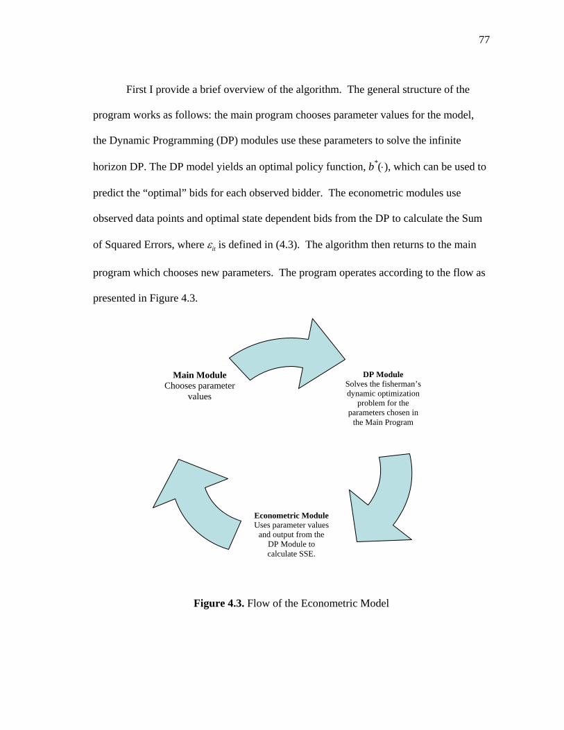
77
First I provide a brief overview of the algorithm. The general structure of the
program works as follows: the main program chooses parameter values for the model,
the Dynamic Programming (DP) modules use these parameters to solve the infinite
horizon DP. The DP model yields an optimal policy function, b*(), which can be used to
predict the “optimal” bids for each observed bidder. The econometric modules use
observed data points and optimal state dependent bids from the DP to calculate the Sum
of Squared Errors, where it is defined in (4.3). The algorithm then returns to the main
program which chooses new parameters. The program operates according to the flow as
presented in Figure 4.3.
Figure 4.3. Flow of the Econometric Model
DP Module Solves the fisherman’s dynamic optimization
problem for the parameters chosen in
the Main Program
Econometric ModuleUses parameter values
and output from the DP Module to calculate SSE.
Main Module Chooses parameter
values
78
It should be noted that the overall set up of the program is general enough to
accommodate different approaches to finding the optimal set of parameters. The method
I use to find the minimum SSE parameter vector is an adaptive grid. Using the adaptive
grid search algorithm a sparse grid is first chosen and then, after observing actual values
found, the grid is refined until the “best possible” parameters are identified. Each time a
grid search is implemented, grids for the parameter are defined in the main module and
the program runs until the SSE for each possible parameter combination has been
evaluated. The combination of parameters with the lowest SSE is the best estimate based
on the optimization criterion. Because of the highly non-linear nature of the objective
function I found the simplicity of the grid search to be quite advantageous. Further,
although more sophisticated nonlinear hill-climbing algorithms might yield more precise
estimates of the parameters, given the parsimonious model specification, such precision
is inconsistent with the true precision of the econometric model.
Grid Search
Using the grid search method, the program evaluates the sum of squared errors at
a number of pre chosen points in order to find that vector which minimizes the chosen
distance measure. This is a computationally intense process but, given the shape of our
objective function, a necessary one. In each iteration of the grid search algorithm, grids
are defined for each of the estimated parameters. A grid is defined by a minimum value,
a maximum value and a number of points between the two to evaluate. For example, if
the y1 grid is defined as having a minimum at 0, a maximum at 10 and 10 grid points then
it can be illustrated by the following vector,
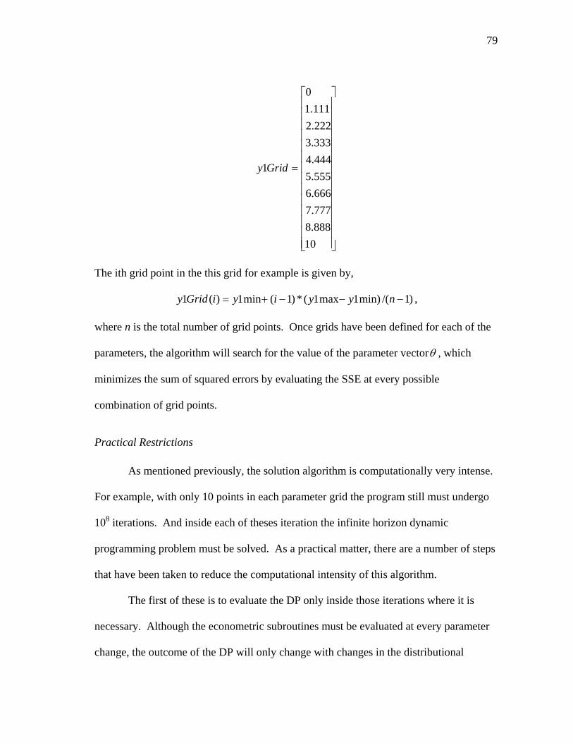
79
10
888.8
777.7
666.6
555.5
444.4
333.3
222.2
111.1
0
1Gridy
The ith grid point in the this grid for example is given by,
)1/(min)1max1(*)1(min1)(1 nyyiyiGridy ,
where n is the total number of grid points. Once grids have been defined for each of the
parameters, the algorithm will search for the value of the parameter vector , which
minimizes the sum of squared errors by evaluating the SSE at every possible
combination of grid points.
Practical Restrictions
As mentioned previously, the solution algorithm is computationally very intense.
For example, with only 10 points in each parameter grid the program still must undergo
108 iterations. And inside each of theses iteration the infinite horizon dynamic
programming problem must be solved. As a practical matter, there are a number of steps
that have been taken to reduce the computational intensity of this algorithm.
The first of these is to evaluate the DP only inside those iterations where it is
necessary. Although the econometric subroutines must be evaluated at every parameter
change, the outcome of the DP will only change with changes in the distributional

80
parameters, g and sigma, which affect the state equation in the DP model. A short
discussion of why this is so follows.
The optimal bid, b*, is a function of the state variables RPLo, RPSpread, and R.
In practice, the DP is actually solved for a small number of possible states and
Chebychev polynomial approximation is used to smooth the value function over the full
range of state variables. The solution to the DP problem yields a b* matrix which
contains an optimal bid as a function of each combination of the possible states. The
econometric subroutine uses linear interpolation to determine which element of this b*
matrix is relevant for a particular bidder. This means that changes in the parameters of
the R function (y1, y2, c1, c2) don’t affect the calculation of the b* matrix, they
determine which element of that matrix is used for a particular bidder. The parameters g
and sigma, because they affect the state transition of the DP, have an affect on the one-
period ahead value function 1tV . Therefore, changes in these parameters will affect the
calculation of the b* matrix. It is therefore possible to economize on run time by calling
to the DP module only for values of which contain changes in g or sigma.
Another way efficiency is promoted in the algorithm is by imposing a theoretical
restriction on the parameter c2. Recall that the benefit function in our model is written as
xccxpypypxR 2121),( ,
and that the parameter c2 reflects that portion of costs that are dependent on vessel
length. In the estimation I impose the restriction 2 0c which saves run time by only
searching for optimal values of c2 in the positive direction. In the adaptive search
algorithm, the approach was to focus first on those parameters for which the value
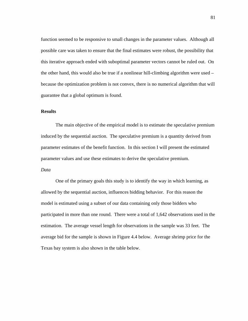
81
function seemed to be responsive to small changes in the parameter values. Although all
possible care was taken to ensure that the final estimates were robust, the possibility that
this iterative approach ended with suboptimal parameter vectors cannot be ruled out. On
the other hand, this would also be true if a nonlinear hill-climbing algorithm were used –
because the optimization problem is not convex, there is no numerical algorithm that will
guarantee that a global optimum is found.
Results
The main objective of the empirical model is to estimate the speculative premium
induced by the sequential auction. The speculative premium is a quantity derived from
parameter estimates of the benefit function. In this section I will present the estimated
parameter values and use these estimates to derive the speculative premium.
Data
One of the primary goals this study is to identify the way in which learning, as
allowed by the sequential auction, influences bidding behavior. For this reason the
model is estimated using a subset of our data containing only those bidders who
participated in more than one round. There were a total of 1,642 observations used in the
estimation. The average vessel length for observations in the sample was 33 feet. The
average bid for the sample is shown in Figure 4.4 below. Average shrimp price for the
Texas bay system is also shown in the table below.

82
$6,000
$8,000
$10,000
$12,000
$14,000
$16,000
$18,000
$20,000
1 2 3 4 5 6 7 8 9 10 11 12 13 14
Round
Bid
2
2.5
3
3.5
4
4.5
5
Pri
ce
Avg. Bid
Price
Figure 4.4. Average Bid and Price by Round in the TX Shrimp License Buyback
Auction
Source: TPWD
Parameter Estimates
Parameter estimates were obtained through the grid search algorithm by running
the estimation program many times and tightening the bounds of selected grids on each
run. In practice it simply was not feasible to chose wide bounds for each grid and allow
the algorithm to search over a large number of grid points for the optimal solution. With
8 parameters even evaluating the model at ten grid points in each dimension would
require 108 iterations. At the current rate of 0.03 seconds per iteration, running the
model with 8 parameters and 10 grid points would require roughly 833 hours of
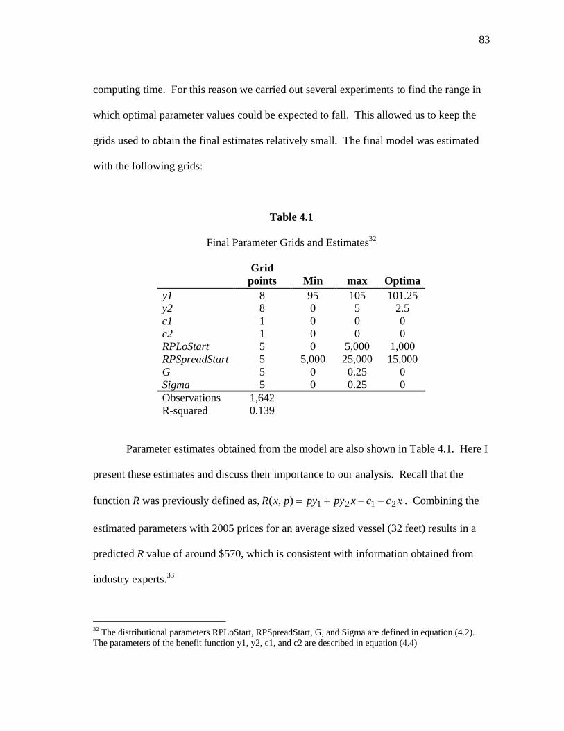
83
computing time. For this reason we carried out several experiments to find the range in
which optimal parameter values could be expected to fall. This allowed us to keep the
grids used to obtain the final estimates relatively small. The final model was estimated
with the following grids:
Table 4.1
Final Parameter Grids and Estimates32
Grid
points Min max Optima y1 8 95 105 101.25 y2 8 0 5 2.5 c1 1 0 0 0 c2 1 0 0 0 RPLoStart 5 0 5,000 1,000 RPSpreadStart 5 5,000 25,000 15,000 G 5 0 0.25 0 Sigma 5 0 0.25 0 Observations 1,642 R-squared 0.139
Parameter estimates obtained from the model are also shown in Table 4.1. Here I
present these estimates and discuss their importance to our analysis. Recall that the
function R was previously defined as, xccxpypypxR 2121),( . Combining the
estimated parameters with 2005 prices for an average sized vessel (32 feet) results in a
predicted R value of around $570, which is consistent with information obtained from
industry experts.33
32 The distributional parameters RPLoStart, RPSpreadStart, G, and Sigma are defined in equation (4.2). The parameters of the benefit function y1, y2, c1, and c2 are described in equation (4.4)

84
In addition to this informal model validation we also have a goodness of fit
statistics. The measure chosen for this model is the 2R statistic. 2R measures the
proportion of the sample variation in actual bids which is explained by the model and is
calculated as,
i tit
i tit
i titit
bbbb
bbbb
R22
2
2
*)*()(
*)*)((
The 2R statistic shows that our model explains almost 14% of the sample variation in the
bids. Considering the parsimonious specification of the model and complexity of the
decision making environment 139.02 R is promising.
Model Validation
The structure of this model – a dynamic programming problem nested within an
outer minimization algorithm – does not lend itself easily to conventional hypothesis
testing. However, the quality of the empirical model can be analyzed by consulting a
variety of somewhat primitive measures.
33 In personal conversations with Robin Reichers of the Coastal Fisheries Division of Texas Parks and Wildlife he has relayed his feeling that many of the bidders in this auction were suffering from poor returns.

85
Model Performance
I have shown that the optimal parameter estimates obtained from the grid search
method explain roughly 14% of the total sample variation in bids. In addition to the R-
squared measure, examining the difference between actual and predicted bids will also
give a sense of how well the model fits.
In Table 4.2 below I show the mean absolute error (MAE) by bid number.
Because it is assumed that information is gained only through bidding, it makes sense to
express the deviations between observed bids and predicted bids in terms of bid number
rather than round.34
Although the difference in actual versus predicted bids is initially quite high, the
model performs relatively well after the first bids. The overall MAE for the entire
sample is 50.1% of observed bids, which may seem high, however it should be
remembered that the computational intensity of this estimation procedure forces us to
search for optima over very course grids.
34 To reiterate: the model treats a bidder participating in the auction for the first time as an uninformed bidder, even if this first bid is placed in the 13th round.

86
Table 4.2
Mean Absolute Error by Bid Number
Bid
Number Observations MAE MAE (%)
1 624 $6,225.91 65.8%
2 624 $2,995.60 47.0%
3 220 $2,813.91 37.0%
4 89 $2,136.33 28.2%
5 37 $3,291.09 27.8%
6 19 $3,869.09 31.7%
7 9 $4,071.67 43.2%
8 7 $4,622.62 28.3%
9 5 $3,880.24 24.3%
10 5 $2,324.53 23.9%
11 2 $3,676.99 32.7%
12 1 $926.19 14.2%
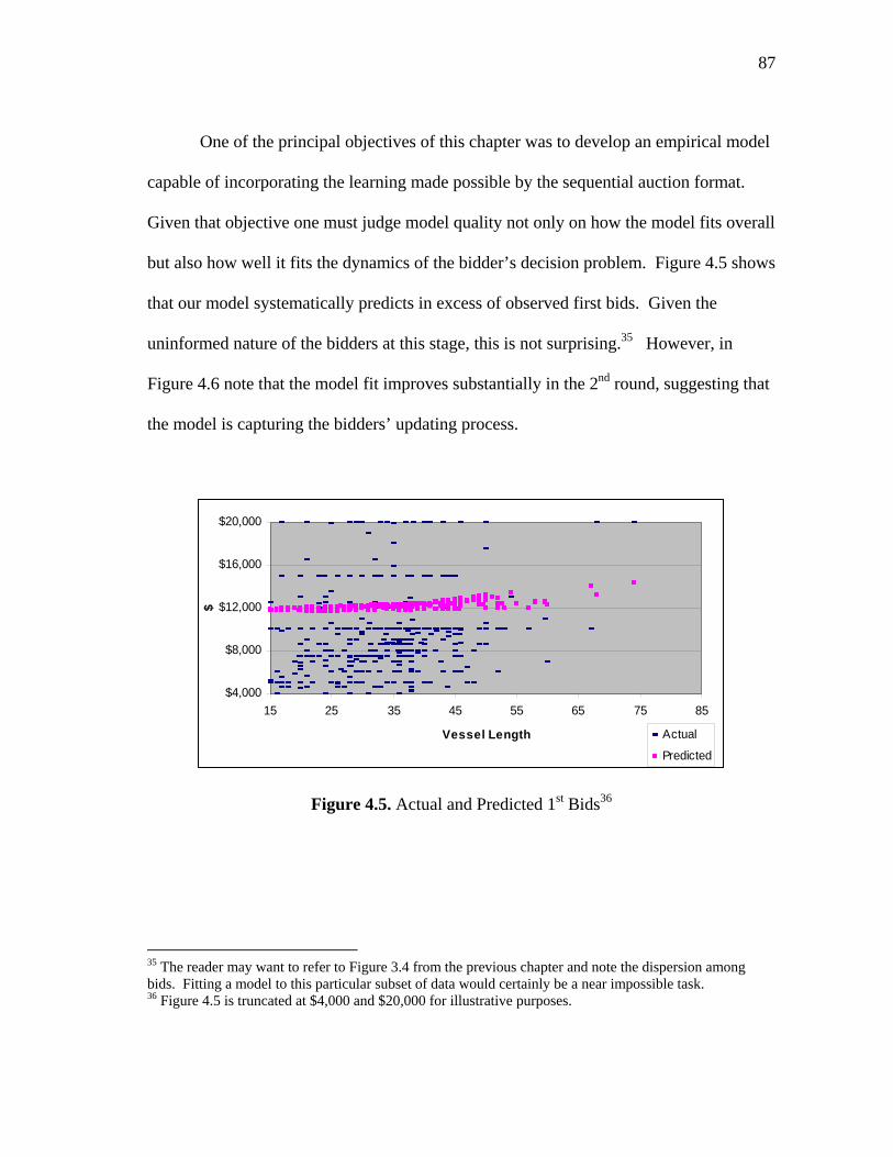
87
One of the principal objectives of this chapter was to develop an empirical model
capable of incorporating the learning made possible by the sequential auction format.
Given that objective one must judge model quality not only on how the model fits overall
but also how well it fits the dynamics of the bidder’s decision problem. Figure 4.5 shows
that our model systematically predicts in excess of observed first bids. Given the
uninformed nature of the bidders at this stage, this is not surprising.35 However, in
Figure 4.6 note that the model fit improves substantially in the 2nd round, suggesting that
the model is capturing the bidders’ updating process.
$4,000
$8,000
$12,000
$16,000
$20,000
15 25 35 45 55 65 75 85
Vessel Length
$
Actual
Predicted
Figure 4.5. Actual and Predicted 1st Bids36
35 The reader may want to refer to Figure 3.4 from the previous chapter and note the dispersion among bids. Fitting a model to this particular subset of data would certainly be a near impossible task. 36 Figure 4.5 is truncated at $4,000 and $20,000 for illustrative purposes.

88
$4,000
$8,000
$12,000
$16,000
$20,000
15 25 35 45 55 65 75 85
Vessel Length
$
Actual
Predicted
Figure 4.6. Actual and Predicted 2nd Bids
Standard Errors of the Point Estimates
A complicating feature of this model is that the DP must be re-run for each
change in RPLo, RPSpread, g, or sigma. Because of this structure it is very costly (in
computing time) to improve the precision around estimates for these parameters. As a
result, estimates for these distributional parameters are not likely to be robust to small
changes in the sample and little meaning could be attached to standard errors.
To ensure that the best estimates for these parameters within the feasible search
range have been selected I perform a check on the objective function values in the RPLo
and RPSpread dimensions. Figures 4.7 and 4.8 show the top 200 objective function
values and the associated RPLo and RPSpread values.

89
-78,000
-77,500
-77,000
-76,500
-76,000
-75,500
-75,000
0 500 1,000 1,500 2,000 2,500 3,000 3,500 4,000 4,500
RPLo
-SS
E
Figure 4.7. Objective Function Values in the RPLo Dimension
-78,000
-77,500
-77,000
-76,500
-76,000
-75,500
-75,000
0 2,000 4,000 6,000 8,000 10,000 12,000 14,000 16,000
RPSpread
-SS
E
Figure 4.8. Objective Function Values in the RPSpread Dimension37
In Figure 4.7 the top 200 objective function value and their associated values for
the parameter PLo are shown. From the figure it is clear that the best objective function
37 For Figures 4.7 and 4.8 the parameters RPLo and RPSpread are defined in equation (4.2)

90
values occur at low RPLo values. Among the grid points that were evaluated in the
RPLo dimension, 1,000 and 1,500 clearly yield the best objective function values.
Figure 4.8 shows the top 200 objective function values and their associated
RPSpread values. Here, the dominance of the RPSpread estimate (over the alternatives)
is pronounced. Note that among the top 200 objective function values only two of the
five points in the RPSpread grid appear (12,000 and 15,000). All other values for
RPSpread evaluated by the grid search algorithm were associated with objective function
values outside the top 200.
In the current set up it is imperative to keep the dimensionality of the problem as
low as possible. To address this need we use very course grids in our search for optimal
values of RPLo and RPSpread. This approach imposes some important limitations in
terms of our ability to express confidence in the quality of estimated parameters. Since
we only evaluate 5 possible values for RPLo and RPSpread we cannot say with certainty
that we have found the best estimates of the true RPLo and RPSpread. With finer
evaluation grids we would almost certainly find RPLo and RPSpread parameters which
offered an improvement over the current estimates. However Figure 4.7 and 4.8
illustrate that, although it may be possible to find better estimates by increasing the
precision of the search algorithm, one would expect these “better” estimates to occur in a
neighborhood around the current estimates. That is, due to the limitations associated
with the nested DP structure of our model, I cannot say that our RPLo and RPSpread
estimates are necessarily the best, however the estimates are certainly the best among all
evaluated alternatives.

91
Because the model involves solving a DP problem for changes in the parameter
space the precision around estimates of RPLo, RPSpread, g, or sigma cannot be
increased without increasing run-time dramatically. For estimates of the parameters of
the R function however, it is possible to use finer grids in the search algorithm at low
cost, making it possible to calculate standard errors around the estimates for y1 and y2.
Greene (2003) shows how standard errors can be calculated for Maximum
Likelihood estimates. Although the estimator used here is the minimization of the sum
of squared errors and not the maximization of a likelihood function, I will show that the
following approach can be used to derive standard errors for this model as well.
The general approach is to use the inverse of the information matrix to calculate
these standard errors. The asymptotic covariances are given by the expected values of
the second-derivitives of the likelihood function.
vectorparameter therepresents where
'
)()]([
21
LEI
The estimator for the asymptotic covariance matrix is computed by evaluating the actual
second derivatives at the optimal parameter values.
'
)()(
^^
^21^^
LI
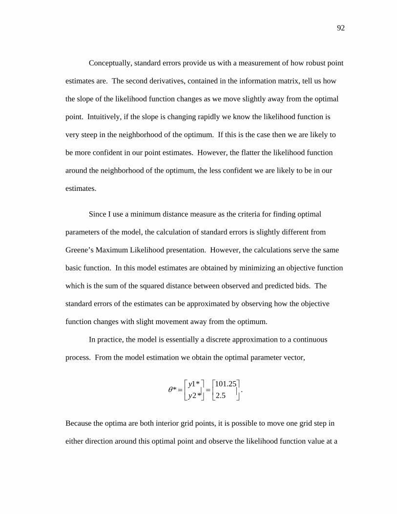
92
Conceptually, standard errors provide us with a measurement of how robust point
estimates are. The second derivatives, contained in the information matrix, tell us how
the slope of the likelihood function changes as we move slightly away from the optimal
point. Intuitively, if the slope is changing rapidly we know the likelihood function is
very steep in the neighborhood of the optimum. If this is the case then we are likely to
be more confident in our point estimates. However, the flatter the likelihood function
around the neighborhood of the optimum, the less confident we are likely to be in our
estimates.
Since I use a minimum distance measure as the criteria for finding optimal
parameters of the model, the calculation of standard errors is slightly different from
Greene’s Maximum Likelihood presentation. However, the calculations serve the same
basic function. In this model estimates are obtained by minimizing an objective function
which is the sum of the squared distance between observed and predicted bids. The
standard errors of the estimates can be approximated by observing how the objective
function changes with slight movement away from the optimum.
In practice, the model is essentially a discrete approximation to a continuous
process. From the model estimation we obtain the optimal parameter vector,
5.2
25.101
*2
*1*
y
y .
Because the optima are both interior grid points, it is possible to move one grid step in
either direction around this optimal point and observe the likelihood function value at a
93
total of 9 points. Figure 4.9 below shows the points of evaluation and the numerical
derivatives associated with each.
In the figure below we have .1031 and ,25.1011,5.991 321 yyy The three
points for y2 are .75.32 and ,5.22,25.12 321 yyy At each of these points we have
an objective function value, which is the sum of squared errors. Using the standard
expression for the log likelihood function of estimator with error variance 2 ,
2
22
2
)')(()2log(
2),(
XyXynLL
(4.5)
we can transform objective function values into log likelihood values and use the inverse
of the information matrix to calculate standard errors.
First note that in the classic linear model the sum of squared errors associated
with estimator is )')(( XyXy . Also, an unbiased estimator of 2 is given by
Kns i
i
2,
where i is the error associated with observation i, n is the number of observations and K
is the degrees of freedoms. By substituting the quantities 2s and SSE into (4.5) it is
possible to transform the SSE values at each grid point into log likelihood values.
Looking along the rows of the matrix in Figure 4.7, one can see the partial
derivatives with respect to y1. Starting in the first cell and moving across the first row,
one can see the 3 values of y1 which are used – one value on either side of the optimal
94
point (101.25). Moving across this row, y2 remains constant and 2 partial derivatives
can be calculated from these three points. Starting in the first cell and moving down the
first column, one can see the representations for two partial derivatives with respect to
y2, evaluated at the first y1 value.
Finding the second derivatives 2
2
2
2
2 and
1 y
LL
y
LL
in this case is a simple matter of
taking a second difference around the optimal points, holding all other parameters at their
optimal levels. Denote 12 11
)2,1()2,2(
yy
LLLL
from above as
1
1
dy
dLL
and23 11
)2,2()2,3(
yy
LLLL
as
2
1
dy
dLL
, then the second derivative 2
2
1y
LL
is approximated by,
12
12
11
11
yy
dy
dLL
dy
dLL
38.
The same process is used to approximate2
2
2y
LL
.
38 The reader should note that, because we use uniform grids the distance between any two neighboring points in the grid is equal.
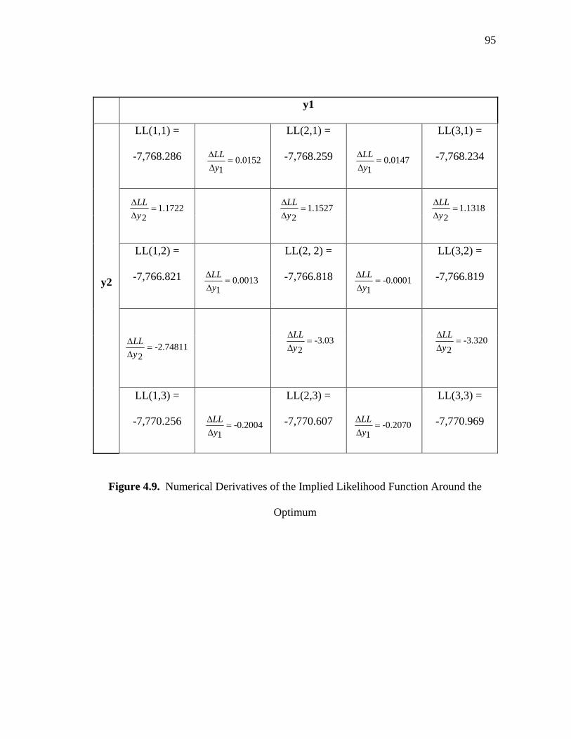
95
y1
LL(1,1) =
-7,768.286
0.01521
y
LL
LL(2,1) =
-7,768.259
0.01471
y
LL
LL(3,1) =
-7,768.234
1.17222
y
LL
1.15272
y
LL
1.13182
y
LL
LL(1,2) =
-7,766.821
0.00131
y
LL
LL(2, 2) =
-7,766.818
-0.00011
y
LL
LL(3,2) =
-7,766.819
-2.748112
y
LL
-3.032
y
LL
-3.3202
y
LL
y2
LL(1,3) =
-7,770.256
-0.20041
y
LL
LL(2,3) =
-7,770.607
-0.20701
y
LL
LL(3,3) =
-7,770.969
Figure 4.9. Numerical Derivatives of the Implied Likelihood Function Around the
Optimum

96
Deriving the cross-partial derivatives for the information matrix, 21
2
yy
LL
and
12
2
yy
LL
, is slightly more complex. To calculate these values I use the change in the
average partial derivatives. For example, to get the cross-partial derivative of y1 with
respect to y2 I use the following procedure:
With 3 values for both parameters there are 2 numerical partial derivatives at each
value of y2 – for y2 = 1.25 the partials are 12 11
)1,1()1,2(
yy
LLLL
and
23 11
)1,2()1,3(
yy
LLLL
.
Averaging these slopes gives an approximation to 25.121
yy
LL, which measures the
change in the likelihood function with a change in y1, holding y2 = 2.5. Averaging in
this manner again for y2 = 2.5 and y2 = 3.75, gives 3 partial derivatives which can be
differenced to provide an estimate for the cross-partial derivative, 12
2
yy
LL
.

97
2
11
2
11
2
1
21
1)75.32(
12
11
)3,1()3,2(
11
)3,2()3,3(
1)5.22(
12
11
)2,1()2,2(
11
)2,2()2,3(
1)25.12(
12
11
)1,1()1,2(
11
)1,2()1,3(
2312
2
31223
21223
11223
y
y
LL
y
LL
y
y
LL
y
LL
yy
LL
y
LLy
y
LLyy
LLLL
yy
LLLL
y
LLy
y
LLyy
LLLL
yy
LLLL
y
LLy
y
LLyy
LLLL
yy
LLLL
Here I have provided some technical details of our numerical approach to
deriving the information matrix. As an inherently numerical process the notation
deviates somewhat from the standard textbook presentation of standard error
calculations. However, the reader should understand that this approach serves the same
purpose as traditional standard error reporting – namely, to understand how the objective
function is behaving in a neighborhood around the optimal parameter estimates.
The table below provides estimates of the asymptotic covariance matrix of y1 and
y2. The matrix of second derivatives contains very large values, suggesting that the
objective function is steep in the neighborhood of the optimal estimates. This gives
estimated standard errors for y1 and y2.

98
Table 4.3
Standard Errors of the Parameter Estimates39
Y1 y2
Y1 701.09
Y2 0.18
The standard errors shown in Table 4.3 suggest that the estimate for y2 is very
robust, while the estimate for y1 is not robust at all. Figure 4.10 shows the 200 best
objective function values in the y1 dimension. From the figure it is clear that the
objective function is not at all responsive to changes in y1 around the optimum.
Figure 4.11 however, shows that the objective function is responsive to changes
in y2. Much like the difficulties discussed previously with attaching confidence to the
grid search estimates of RPLo and RPSpread, it is difficult to say how robust the estimate
of 2.5 for y2 would be to small changes around the value. From Figure 4.11, it is clear
that the best objective function values occur around the point estimate for y2. So again,
although it is not possible to say that the y2 estimate is the true objective function
maximizing value, it is clear that the y2 estimate is the best among all values in the set
which made estimation feasible.
39 The reader may refer to equation (4.4) for definitions of the variables y1 and y2.

99
-78,000
-77,500
-77,000
-76,500
-76,000
-75,500
-75,000
95 96 97 98 99 100 101 102 103 104
y1
-SS
E
Figure 4.10. Objective Function Values in y1 Dimension
-78,000
-77,500
-77,000
-76,500
-76,000
-75,500
-75,000
0 1 2 3 4 5 6
y2
-SS
E
Figure 4.11. Objective Function Values in the y2 Dimension40
40 For Figures 4.10 and 4.11 the parameters y1 and y2 are defined in equation (4.4)
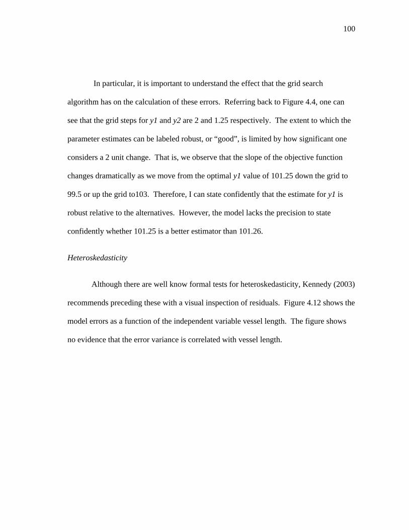
100
In particular, it is important to understand the effect that the grid search
algorithm has on the calculation of these errors. Referring back to Figure 4.4, one can
see that the grid steps for y1 and y2 are 2 and 1.25 respectively. The extent to which the
parameter estimates can be labeled robust, or “good”, is limited by how significant one
considers a 2 unit change. That is, we observe that the slope of the objective function
changes dramatically as we move from the optimal y1 value of 101.25 down the grid to
99.5 or up the grid to103. Therefore, I can state confidently that the estimate for y1 is
robust relative to the alternatives. However, the model lacks the precision to state
confidently whether 101.25 is a better estimator than 101.26.
Heteroskedasticity
Although there are well know formal tests for heteroskedasticity, Kennedy (2003)
recommends preceding these with a visual inspection of residuals. Figure 4.12 shows the
model errors as a function of the independent variable vessel length. The figure shows
no evidence that the error variance is correlated with vessel length.

101
-15,000
-5,000
5,000
15,000
25,000
35,000
0 10 20 30 40 50 60 70 80
Vessel Length (feet)
B - B
* ($
)
Figure 4.12. Prediction Error by Vessel Length
Figure 4.13 shows the model errors as a function of the independent variable
price. For the price variable, prediction errors tend to be higher at the higher price levels.
From figure 4.14, one also notes that the number of observations in the sample appears to
be correlated with the price. This suggests a possible extension to the model. Since 46%
of the total observations in the sample come from the 5 rounds in which shrimp price
exceeded $4/lbs, a sample selection correction may be in order here. Unfortunately, the
numerical intensity of the current model prohibits the introduction of more structure.
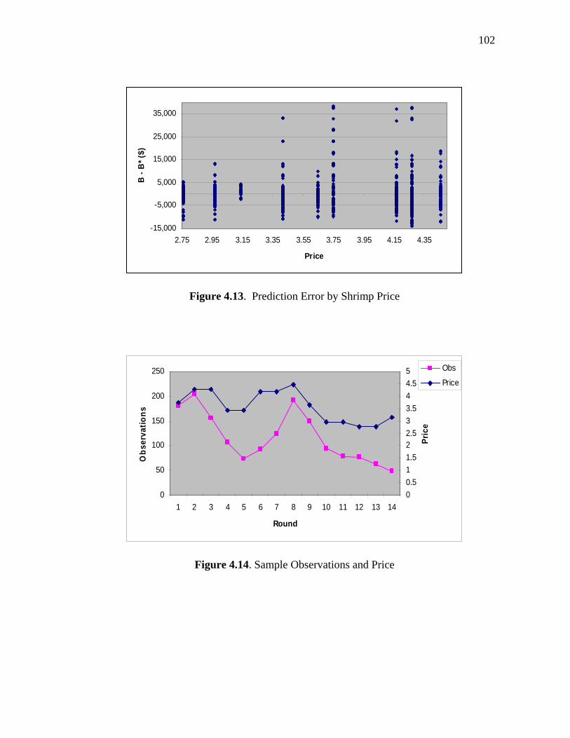
102
-15,000
-5,000
5,000
15,000
25,000
35,000
2.75 2.95 3.15 3.35 3.55 3.75 3.95 4.15 4.35
Price
B -
B*
($)
Figure 4.13. Prediction Error by Shrimp Price
0
50
100
150
200
250
1 2 3 4 5 6 7 8 9 10 11 12 13 14
Round
Ob
serv
atio
ns
0
0.5
1
1.5
22.5
3
3.5
4
4.5
5
Pri
ce
Obs
Price
Figure 4.14. Sample Observations and Price
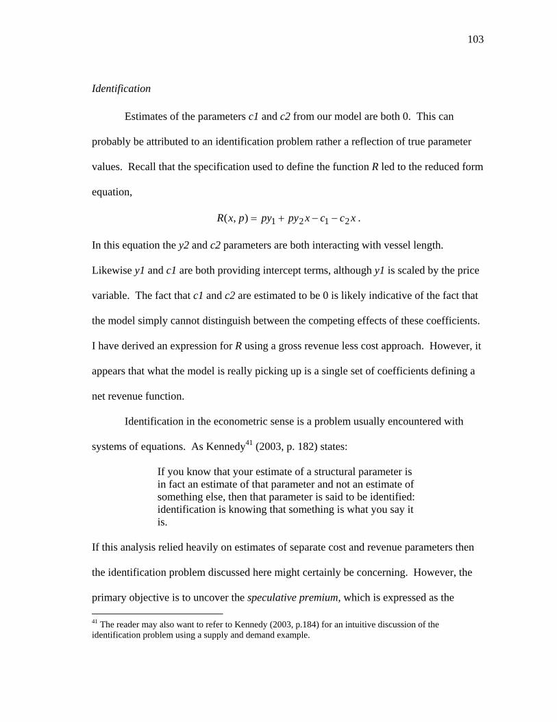
103
Identification
Estimates of the parameters c1 and c2 from our model are both 0. This can
probably be attributed to an identification problem rather a reflection of true parameter
values. Recall that the specification used to define the function R led to the reduced form
equation,
xccxpypypxR 2121),( .
In this equation the y2 and c2 parameters are both interacting with vessel length.
Likewise y1 and c1 are both providing intercept terms, although y1 is scaled by the price
variable. The fact that c1 and c2 are estimated to be 0 is likely indicative of the fact that
the model simply cannot distinguish between the competing effects of these coefficients.
I have derived an expression for R using a gross revenue less cost approach. However, it
appears that what the model is really picking up is a single set of coefficients defining a
net revenue function.
Identification in the econometric sense is a problem usually encountered with
systems of equations. As Kennedy41 (2003, p. 182) states:
If you know that your estimate of a structural parameter is in fact an estimate of that parameter and not an estimate of something else, then that parameter is said to be identified: identification is knowing that something is what you say it is.
If this analysis relied heavily on estimates of separate cost and revenue parameters then
the identification problem discussed here might certainly be concerning. However, the
primary objective is to uncover the speculative premium, which is expressed as the
41 The reader may also want to refer to Kennedy (2003, p.184) for an intuitive discussion of the identification problem using a supply and demand example.
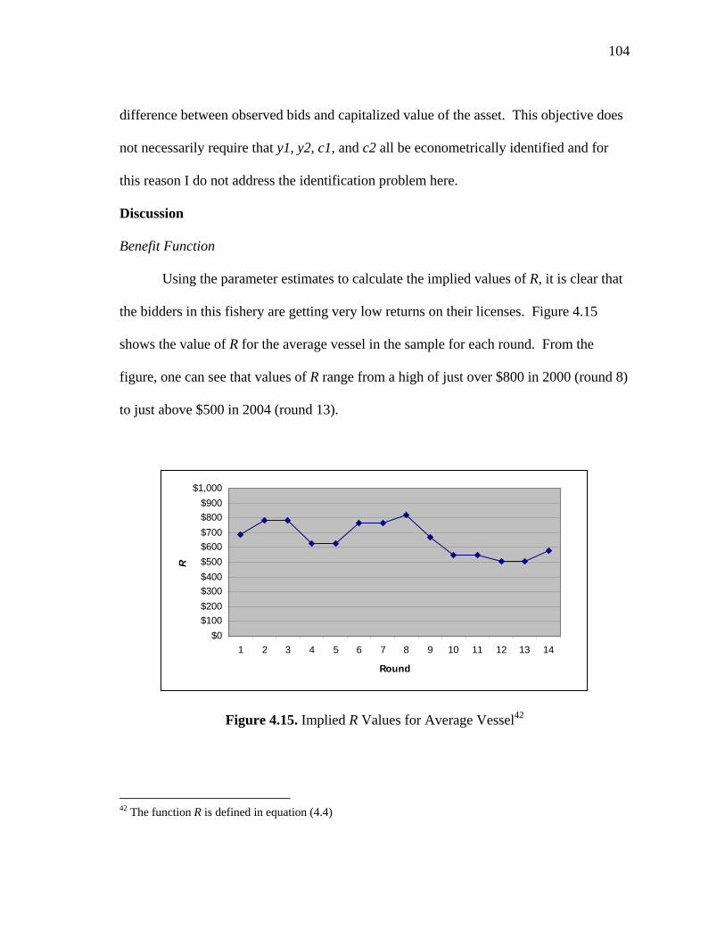
104
difference between observed bids and capitalized value of the asset. This objective does
not necessarily require that y1, y2, c1, and c2 all be econometrically identified and for
this reason I do not address the identification problem here.
Discussion
Benefit Function
Using the parameter estimates to calculate the implied values of R, it is clear that
the bidders in this fishery are getting very low returns on their licenses. Figure 4.15
shows the value of R for the average vessel in the sample for each round. From the
figure, one can see that values of R range from a high of just over $800 in 2000 (round 8)
to just above $500 in 2004 (round 13).
$0
$100
$200
$300
$400
$500
$600
$700
$800
$900
$1,000
1 2 3 4 5 6 7 8 9 10 11 12 13 14
Round
R
Figure 4.15. Implied R Values for Average Vessel42
42 The function R is defined in equation (4.4)

105
The Speculative Premium
The parameters of the R function allow calculation of the speculative component
present in bidding behavior in the sequential auction. Here I present the derivation of the
speculative premium and discuss its significance.
By solving the dynamic decision problem stated in (2) the bidder learns his or her
b* conditional on a set of parameters. And by comparing those conditional b*s with
observed decision the parameter vector * which minimizes the sum of squared errors
was found. With these parameter estimates, we can calculate the implied value of R
which, when compared to observed bids gives the speculative premium.
Figure 4.16 shows the average speculative premium by round for all vessels in
the sample. Figure 4.17 shows the average speculative premium for four representative
vessel lengths based on quartiles of the distribution of all vessel lengths in the fishery.
$0
$2,000
$4,000
$6,000
$8,000
$10,000
$12,000
$14,000
$16,000
1 2 3 4 5 6 7 8 9 10 11 12 13 14
Round
Figure 4.16. Average Speculative Premium by Round for All Vessels

106
$0
$2,000
$4,000
$6,000
$8,000
$10,000
$12,000
$14,000
$16,000
$18,000
1 2 3 4 5 6 7 8 9 10 11 12 13 14
Round
$
14 - 31 ft
32 - 37 ft
38 - 43 ft
> 43 ft
Figure 4.17. Average Speculative Premium by Round and Length Class
From Figure 4.17 one can see that the difference between bid amount and the capitalized
value of the asset (the license) is initially quite volatile. This is consistent with the
hypothesis of agent learning. In the early round, when bidders are still learning about the
agency’s willingness to pay relative to their own valuations, the speculative component
is highly variable. By about halfway through the sample however, it appears that bidders
have settled in to a steady state level of speculation around $6,000.
Summary of Empirical Work
The overarching goal of this chapter was to estimate the magnitude of speculation
present in this sequential buyback auction. This quantity plays a vital role in our cost
benefit analysis of sequential versus one-time auctions, which I present in the next
chapter. However, in defining and estimating a model capable of measuring this
107
speculative component I have also presented several important empirical and
methodological contributions.
One important methodological contribution of this work is the estimator itself.
As was discussed previously, models of this type are often estimated using a maximum
likelihood approach where the likelihood function appears similar to that of a
multinomial logit model. When the control variable is discrete this approach is
appropriate and its use is well documented in the literature (Rust, 1988; Provencher and
Bishop, 1997; Schjerning, 2005 among others). However, in this model the control
variable, bid, is continuous. The difference highlights an important contribution of this
work. Here I have presented a feasible estimator for a dynamic decision model with a
continuous control variable.
The model is also unique in that it incorporates the learning made possible by the
sequential auction into the decision process. I have shown here how a Bayesian updating
procedure can be used to transmit information acquired in the current round and inform
next period’s bidding. The state equation provides a guide for how learning can be
modeled inside of a nested dynamic optimization estimation routine.
Although I have shown some large prediction errors present in the model, in
estimating this model, I believe sufficient evidence has been provided to validate this
approach. In particular, the R-squared measure is higher than might otherwise be
expected, considering the rich decision environment that is explained with only a few
variables. Furthermore, the model’s predictions improve greatly after one realized
outcome, suggesting that the agent’s learning is being appropriately model. And finally,
108
standard errors for the two parameters of the R function are low, suggesting that these
estimates are relatively robust.
In short, although further refinements are necessary to achieve greater precision
on the point estimates, I believe that the results of the estimation are sufficient both to
validate this dynamic econometric approach and provide reasonable estimates for use in
the next chapter’s policy simulation. With respect to this last point, in achieving reliable
estimates for parameters of the R function, I have found that bidders in the sequential
auction do inflate their bids by a speculative premium. This is certainly an important
result for fisheries managers considering using a buyback program for capacity
reduction. However, more generally, it can be stated that the repeated game format of
the sequential auction seems to offer agents an incentive to over bid relative to their true
valuation.

109
CHAPTER V
A COST-BENEFIT ANALYSIS OF SEQUENTIAL
VERSUS ONE-TIME BUYBACK AUCTIONS
Introduction
In their extensive survey of buyback programs Holland, Gudmundsson and Gates
(1999) show that license buyback programs have been a popular management tool for
addressing a range of fisheries management issues including overfishing and
overcapacity. Given the popularity of license buyback programs, it is important to
understand the design and implementation issues of these programs as they relate to
management goals. In this chapter, I study how the key design issue of auction method
will affect the ability of a buyback program to reduce capacity and generate rents in the
fishery.
Once the management authority has decided to implement a license buyback,
they must consider how that program will be carried out, specifically, deciding how these
licenses will be purchased. The two most likely competing candidates here are via an
agency stated price offering or a buyback auction. Under a price offering system, the
agency would simply state a price at which it is willing to buyback licenses and then buy
permits back from as many willing sellers as the budget allows. Under an auction
system, the agency solicits bids from license holders and decides, based on bids and the
management goals, how to allocate the budget among collected bids. Although there are
a number of interesting implications surrounding the auction versus pricing decision,
they are beyond the scope of this analysis. The point of departure for this study will be
110
an agency that has decided to implement a license buyback auction. Readers interested
in a discussion of the relative merits of an agency stated price buyout versus an auction
mechanism should refer to Latacz-Lohmann and Van der Hamsvoort (1997).
The next key design issue that the agency faces is whether the auction will take
place in a single year or over time. The current literature on buybacks exhibits a notable
lack of discussion of this particular issue and there does not seem to be a clear preference
among fisheries managers in the U.S. for one auction type over the other. Of the two
U.S programs discussed in Curtis and Squires (2007), one is a sequential buyback
auction and the other a one-time buyback auction.
Intuitively speaking, from the perspective of the managing agency, an advantage
to one-time license buybacks (OTBs) over sequential buybacks (SBs) is that they remove
the possibility of gamesmanship from the process of buying back permits. By
completing the buyout in a single year the agency does not allow participants to learn
about the agency’s willingness to pay. Intuition and economic theory suggest that this
type of buyback auction should lead to stated buyout prices (bids) that are close to the
individual’s true value.
A notable disadvantage of the OTB relative to the SB is that the OTB requires all
funding up front. With a SB program the agency has the option of generating funds each
year, through a tax for example43, and thereby funding itself. A one-shot program,
however, requires a much larger initial investment. The relative importance of this will
be the focus of our analysis here. Another advantage of a SB program, which will not be
43 The Texas program funds buyouts partially through a fee assessed to the saltwater fishing stamp.
111
evaluated in this chapter, is that it provides the opportunity for managers to learn as the
program proceeds. I discuss that aspect in the concluding comments, but do not formally
evaluate its significance here.
In this chapter I compare two buyback programs with an equivalent pot of money
spent two different ways. I model a SB program with an annual budget that is exhausted
each year over a ten year period and contrast this with a OTB program that has a budget
equal to the present value of the SB’s stream of payments. The setting for these policy
comparisons will be the Gulf of Mexico’s shrimp fishery.
In the next section I provide brief clarification of some terms that will be
important to understand for this analysis. Then I discuss the methodology for this study
and introduce the General Bioeconomic Fisheries Simulation Model (GBFSM) which is
used to simulate policy paths for our analysis. The details of the scenarios considered for
the policy comparisons are then presented. Finally, I present the results of the simulation
and conclusion that can be drawn from the analysis.
Important Terms and Concepts
“License” vs. “Permit”
In this chapter it will be important to understand the distinction between the terms
“license” and “permit.” In the Gulf of Mexico a shrimp license is an asset which confers
on its holder the right to shrimp in state waters only. A permit allows the holder to fish
for shrimp in federal waters. When referring specifically to an asset allowing the holder
to shrimp in federal waters the term “permit” will be used. In all other instances the

112
general term “license” will be used, but will refer to a general license to participate,
rather than a specific limited right to fish in state waters. This is done since the term
“license” (e.g. sequential license buyback), is the term conventionally used in the
fisheries economics literature. However, the reader should understand that comments
about licenses in general also apply to a program buying back permits to fish in federal
waters. When referring specifically to state licenses, I will indicate this.
The Fishery
The Magnuson-Stevens Fishery Conservation and Management Act defines a
fishery as:
one or more stocks of fish which can be treated as a unit for purposes of conservation and management and which are identified on the basis of geographical, scientific, technical, recreational, and economic characteristics.
In this chapter I use the term “fishery” to apply to the various regional shrimp stocks
throughout the Gulf of Mexico as well as the Gulf as a whole. In each of our simulated
programs, “the fishery” will be defined by the management’s authority. For example,
when referring to the Texas Inshore Shrimp License Buyback Program, the term
“fishery” will be used to refer to the inshore shrimp stock in Texas and those licensed to
harvest that resource. In this chapter I will also analyze simulated programs for capacity
reduction in the Gulf of Mexico as whole. The boundaries of “the fishery” will be
assumed to extend as far as the authority of the program in question. Moreover, I use the
term “fishery” to apply only to the harvesting sector. There are no effects on the
processing sector, consumer, or any other direct or indirect impacts modeled here.
113
Methodology
The overarching goal of the analysis in this chapter is to simulate a buyback
program implemented with a SB auction and a program carried out via a OTB auction
and compare their relative abilities to achieve the management goals of reducing
capacity, increasing productivity, and increasing fishery rents. To achieve this goal, I use
results of the analysis of the SB auction that has been used by the Texas Parks and
Wildlife Department (TPWD) to buy back Bay and Bait licenses in the Texas inshore
shrimp fisheries. The TPWD program is an ongoing auction that has been purchasing
bay and bait licenses from inshore shrimpers since 1995.44 Using data from this auction,
certain behavioral patterns can be identified which characterize how fishermen respond
to the incentives of a SB auction. In Chapter IV I estimated a model of bidding behavior
using a dynamic econometric model. The model included an estimate of the speculative
premium. In the previous chapter I also presented the details of that econometric model
and the nested dynamic optimization algorithm used to obtain parameter estimates of that
model.
In this chapter I use the results from Chapter IV to simulate bidding behavior in a
buyback program for large vessel permits throughout the Gulf of Mexico using both a SB
and OTB auction. With these simulations it is possible to compare the cost and
effectiveness of each. The speculative premium is the key variable in this chapter as it
44 Further background on the Texas Program can be found in the third chapter of this dissertation as well as Funk et al. (2003).
114
establishes a behavioral relationship between the value that a fisherman attaches to their
license and the bids that he or she will offer for the sale of that asset.
A GBFSM Introduction
To conduct the simulations necessary for this study I developed a policy module
which operates inside of the General Bioeconomic Fisheries Simulation Model
(GBFSM). GBFSM has been discussed at length in the fisheries economic literature and
a detailed discussion of the model is beyond the scope of the current analysis. In this
section we will provide a very general overview of GBFSM and discuss the placement of
the Gulf of Mexico license buyback module within the overall structure. For a more
detailed discussion of GBFSM the reader should consult Grant and Griffin (1979) and
Grant, Isakson, and Griffin (1981).
GBFSM is a multi-species, bioeconomic simulation model developed by Dr.
Wade Griffin. A summary of the major functionality of the simulation model is provided
in the GBFSM manual:
The biological sub-model represents the recruitment of new organisms into the fishery by species, sex, and fishing area. Recruitment may be in one or all depth zones, and movement may be to greater or lesser depths and between fishing areas. Organisms grow and move from one size class to another, and mortality results from both natural causes and fishing…
… The economic submodel represents the fishing effort (nominal days fished converted to real days fished) exerted on each species and on by-catch. Monetary costs of fishing, value of harvest, and rent to the fishery are calculated.

115
Fleets
This simulation model divides the Gulf of Mexico into four regions as shown
below in Table 5.1.
Table 5.1
Four Gulf Regions of Shrimp Landings in the General Bioeconomic Fisheries
Simulation Model 45
Region 1 Region 2 Region 3 Region 4
Florida Alabama46, Mississippi, &
Eastern Louisiana
Western Louisiana
Texas
Each region includes two vessel classes: vessels less than 60 feet in length and
vessels 60 feet or greater in length. In the model, small vessels (those less than 60 feet)
generally shrimp in inshore areas in state waters and offshore state waters.47 Large
vessels shrimp both in offshore state waters and federal waters, including the Exclusive
Economic Zone (EEZ). The model is calibrated so that the initial size of each large
vessel fleet is equal to the number of federal permits requested from each region in 2005.
45 Regions are where shrimp are landed and areas are where shrimp are caught. Areas are adjacent to each region. It is assumed that vessels land fish in only one region but can catch fish in any of the four areas where shrimp are caught. 46 In the results section of this chapter I will refer to each region by its proper name. For example, I will refer to “Texas” instead of “region 4.” As a convenience to the reader however, I will refer to region 2 as “East Gulf.” 47 There are only a few small vessels that have permits to fish in federal waters, however for convienence it is assumed that small vessels do not have permits.

116
An important assumption of the model is that large vessels selling back their federal
permits do not continue fishing in offshore areas in state waters48.
Finally, it deserves mention that GBFSM is a homogenous fleet model. Revenue
and cost figures are calculated by region and vessel class. This means that all vessels
within a particular fleet are treated as if they have the same revenue and cost structure.
The buyback policy module works in four basic steps. First, using the estimated
speculative premium in the SB program and fishery rents, which are calculated in
GBFSM’s economic submodel, the distribution of bids that will be submitted to the
auction in a given year is predicted. Next, the budget determines how many of these bids
can be accepted. The size of the fleet is then adjusted to reflect the number of licenses or
permits exiting the fishery due to the buyout. Finally, effort in days fished is adjusted
according to the new fleet size. The next section will explore these steps individually.
The GBFSM Buyback Policy Module
The buyback policy module was written in Fortran 90 for this analysis and
functions as one of several GBFSM policy options. The module operates inside of
GBFSM and uses information obtained from GBFSM’s biological and economic
submodels, along with data from outside the model, in order to simulate the effects of
different buyback programs. This section discusses the details of the buyback policy
module.
48 From personal communication with Mike Travis of NMFS I understand that it would not be economically viable for large vessels to operate without access to the EEZ. Therefore, I believe it is reasonable to assume that large vessels forfeiting their federal permits are not continuing to shrimp in offshore state waters.

117
Data
The data required of GBFSM for our simulations can be broken into two classes.
The first class of data provides the policy module with a complete description of the
programs it must simulate. The second class of data deals with parameters estimates and
other data obtained from outside of GBFSM and used by the buyback policy submodel.
The program description data starts with a specification of the number of
programs to be simulated. Next, the region/vessel class combinations eligible to
participate in each program must be defined. Then each program is assigned a type
(either sequential or one-time). Finally, the total budget for each program is declared.
The second class of data includes estimated values from outside the simulation model.
The first of these is the speculative premium. This value can be calculated using the
parameters of the function estimated in Chapter IV for each region, vessel class, and
year. Next, the actual number of vessels in each region/vessel class combination must be
input.
Initial Values
GBFSM is set up to analyze percent changes in fleet size. The simulation model
treats each region as if it were initially composed of 100 representative vessels. For the
offshore fisheries, the buyback policy module keeps track of the representative fleet
(percent of original vessels) in each year as well as the actual fleet and this translates into
a corresponding percentage reduction in the total effort available to fish in each region.
For the inshore fisheries, the model only tracks percentage changes in each fleet. I do
not track changes in actual vessels for the inshore fisheries because of the lack of reliable

118
data on the number of inshore vessels for each region. However, the absence of actual
vessel numbers for the inshore fisheries should not qualitatively limit the analysis.
Because offshore fishing in state waters is a relatively minor part of the fishery,
in all of the analysis in this chapter it is assumed that any program that retires the federal
permits will effectively also retire the state off-shore license. No program explicitly for
state offshore fishing is modeled. In the model, vessels are assumed to land shrimp in a
single region. For calibration, individual vessels are not identified, so there is a one-to-
one relationship between the landings in the region and the vessels.
Predicted Bids
The first major task carried out in the buyback policy submodel of GBFSM is to
determine a distribution of bids for each fleet. Bids are determined based on the
profitability of the fishery and type of buyback under analysis. To present this
calculation completely it will be informative to back-up and briefly discuss order of
operations.
Figure 5.1 illustrates the important steps to understand for this analysis. When a
simulation run begins, the model initializes several key variables, including fleet size.
The simulation then runs through the biological submodel, which calculates recruitment,
mortality, and other important biological relationships. Once the biological variables are
calculated, the simulation then calculates economic variables such as cost and fisheries
rents. Of particular interest for this analysis are fishery revenues and the cost structure.
After calculating the key economic variables, the simulation enters the license buyback
submodel.
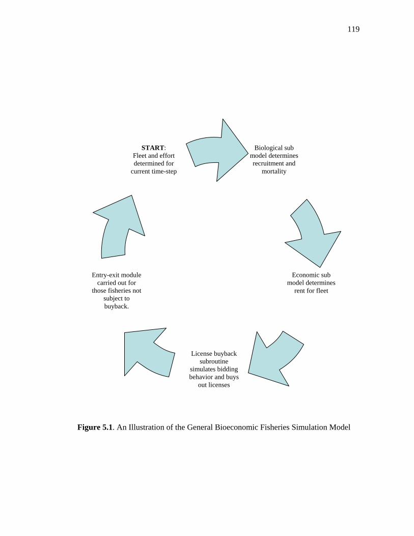
119
Figure 5.1. An Illustration of the General Bioeconomic Fisheries Simulation Model
Biological sub model determines recruitment and
mortality
Economic sub model determines
rent for fleet
Entry-exit module carried out for
those fisheries not subject to buyback.
License buyback subroutine
simulates bidding behavior and buys
out licenses
START: Fleet and effort determined for
current time-step
120
In a given year, the model enters the buyback policy module with values for the
crucial variables, fleet size and net revenue. To predict the bids that will be submitted
for license buyout in a SB auction I use the net revenue combined with the estimated
value of the speculative premium. And to predict bids in a OTB auction I use the present
value of net revenues. Net revenues are defined as revenues net of all variable costs.
From the econometric model discussed in Chapter IV we have estimates for the
speculative component. The following details how the estimates of speculation are used
to predict bids for the simulation model.
Denote the benefit function for an individual with vessel length x facing price p
as R(x,p) and the optimal bid as b* then the speculative ratio for vessel length x in time t
is,
.),(
*),(
tpxR
btxspecratio
This ratio is used to calculate the average bid for a vessel class for the SB programs in
the license buyback submodel.
At the point in the overall simulation when the program enters the buyback policy
module, a value for net revenue by region and by vessel class has already been
calculated. Under the assumption that revenues and costs are distributed evenly
throughout the fleet the expected net revenue for individual i can be calculated as,
.),(
),(
classvesselregionfleet
classvesselregionnetrevenuenetrevenuei
121
In a OTB auction theory suggests that an individual’s minimum willingness to
accept payment for a license will be the present value of that asset. So for the OTB
auction the average bid is calculated as,
, where the discount factor.1
OTB ii
netrevenuebid
In the SB auction however the average bid will contain a speculative component.
We calculate the average bid for the SB auction as,
* (1 ).1
SB ii i
netrevenuebid specratio
The average bid shown above is the bid per vessel for each region and vessel
class. This is converted to a bid per percent of the fleet by adjusting the per vessel bid by
the ratio of actual vessels to representative units.
Once the mean bid per percent of the fleet has been calculated, bids for the
vessels in that fleet are determined by generating a distribution around the average as
follows. I assume that bids from the fleet will be distributed logistically around the
average bid, which gives a closed form expression for the cumulative density function
(cdf),
k
mb
e
bD)(
1
1)(
.
Here, the parameter m represents the mean of the distribution and k is a distributional
parameter related to the variance (the parameter k is defined below).
With this assumption about the distribution of the bids, it is possible to calculate
the bid at a given percentile of the fleet, p, by inverting the cdf,
122
ln 1b m k p p .49 (5.1)
The parameter k defines the standard deviation of the distribution as follows
3.14159.where
3
3
1
2
2
222
k
k
The variance, 2, is estimated based on data from the TPWD program as is discussed in
section entitled “Bidding Assumptions” below.
Table 5.2 shows a sample distribution for a fleet with 100 vessels. Here the
average bid is $10,000 and standard deviation is $3,000. The table shows predicted bids
from this fleet.
Bid Acceptance
Once the distribution for bids submitted to the buyback auction has been
simulated, we must determine what percent of the fleet can be purchased. In the
simulations this decision is based on available funds (recall that the funds available are
exogenous and predetermined). The simulation model can accommodate a variety of
different combinations of region and vessel classes eligible to participate in the program
and one or several programs can be operating simultaneously. For example, it is possible
to simulate one program for the entire gulf or a program for each region in the gulf. Each
region-vessel class combination in a program is called a group and for each group there
49 For example, the 90th percentile, p=0.9, would refer to the vessel whose bid is higher than 90% of the bids in the fleet.

123
is a separate distribution of bids. The bids from all groups in a program are sorted from
lowest to highest and the lowest bids are accepted until the available funds are exhausted.
Table 5.2
Sample of a Simulated Distribution of Bids
Vessel P
Bid50
p
pkmb
1ln
1 0.01 $2,399.73 2 0.02 $3,562.98 3 0.03 $4,250.58 4 0.04 $4,743.54 5 0.05 $5,129.94 6 0.06 $5,449.00 7 0.07 $5,721.65 8 0.08 $5,960.39 9 0.09 $6,173.28 10 0.1 $6,365.82
98 0.98 $16,437.02 99 0.99 $17,600.27
To provide an example of the bid/buyout portion of the algorithm, suppose one
wanted to simulate the capacity reduction achieved by extending the current Texas
program (call this program 1) and also adding a buyback program for all large, federally
permitted vessels in the gulf (call this program 2). The current Texas program applies
only to the Texas Bay System, therefore, this program would have one group (Region 50 Bid, as used here, is defined in equation 5.1.

124
4/vessel class 1). The second program, operating in the gulf, would have 4 groups
(Region 1/vessel class 2, Region 2/vessel class 2, Region 3/vessel class 2, and Region
4/vessel class 2).
For program 1 the buyout process is simple. The simulated distribution gives a
dollar amount at each percent of the fleet that is required to buyout that percent. With
only one group in the program one could simply integrate along this distribution until the
budget is exhausted.
For program 2, however, the buyout process is more complex. With 4 groups
eligible to participate there are 4 separate distributions of bids. The model will pool
these bids and sort them in ascending order. It will then begin purchasing the cheapest
license until the budget is spent. It is interesting to note here that with this type of
program it is possible to have regions from which no licenses are purchased.
Fleet/Effort Updating
The last step in the buyback module is to update the fleets and return these values
back to the main GBFSM model for use in the next time step. After the bid acceptance
portion of the buyback module is complete we know the percent of each fleet that was
bought out via the simulated programs. The fleet is then adjusted by this percent. Fleet
updating is a simple matter of multiplying the fleet at the beginning of the year by one
minus the percent reduction. Likewise, effort, measured in days-fished, is adjusted by
the percent change in the fleet.

125
Important Assumptions of the Simulation Model
The simulation model in general and the policy module in particular impose some
important limitations on the results. It is important to be transparent about these in order
for the reader to understand what this model is and is not capable of analyzing. What I
believe to be the most important assumptions underlying our model are discussed
below.51
Unit Costs and Prices
One important assumption relating to the fleet rent function is that unit prices
within a size category and unit costs are unchanging. The model holds prices and unit
costs constant at 2005 levels throughout the 10-year simulation. This is an important
assumption because as licenses are bought back capacity leaves the fleet, which may
affect shrimp supply. One possible effect of this shift in the supply curve is higher
shrimp prices. This movement is not captured in our model.52
Bidding Assumptions
In applying the bidding distribution there are two assumptions that deserve some
discussion. This first is that there exists a minimum price, below which nobody will bid
regardless of rents. The second is that the standard deviation of the distribution is
declining through time.
51 A discussion of the assumptions that are maintained in GBFSM can be found at the GBFSM website: http://agecon2.tamu.edu/people/faculty/griffin-wade/gbfsm/ 52 It should be noted however that prices do rise during the 10-year simulation. The price rise is due to a rise in the average size of shrimp harvested as effort decreases. Since prices are positively related to shrimp size, average shrimp price does rise over the 10-year simulation.
126
The assumption of a minimum bid stems from the estimation work and is
empirically justified. The estimation of the bid function for Texas fishermen includes a
variable for the minimum point in the bidder’s subjective expected grant distribution.
This is the lowest value for which bidders in that auction believe the probability of
having the agency accept their bid is 1. In this study the value is captured by the variable
PLoStart, which is a variable to be estimated. This variable is the first prior expectation
over the lowest point in the grant distribution. The estimate of this variable (from
Chapter IV) was $1,000. This suggests that bidders in the Texas auction who have, as of
yet, no knowledge of prices paid for licenses are behaving as though $1,000 is the
minimum license price.
In order to use this estimate to inform the simulations, it is converted to a bid per
unit length figure then multiplied by a factor representing each region’s rents in relation
to Texas. The data from the Texas program included bidding behavior almost
exclusively from small inshore vessels. Since the simulations in this chapter deal with
large offshore vessels, the observed bid floor was converted to a bid floor in terms of
dollars per foot of vessel length by scaling up. The bid floor is applied to large vessels
by multiplying by 60, the lower bound for length of large boats in GBFSM. The regional
rent factor is calculated simply as the ratio of fishery returns in region i to fishery returns
in Texas. This is meant to try and capture some of the regional differences in bidding
that may arise because of differing economic conditions.
Another key component of the calculation of the distribution of bid is the
standard deviation. I have shown that over time the distribution of the bids from the
127
Texas auction condensed considerably. Over the life of that auction the standard
deviation in the distribution of bids went from around $20,000 down to $6,000. I use
this trend in the standard deviation for the Texas auction to help form assumptions about
the standard deviations for the simulated bid distributions.
At $20,000 the standard deviation in the Texas inshore auction is about 5.3 times
the average bid in that auction. This deviation declines by an average of 7% per year
through the 8th year. Therefore, in the first period of each simulation the standard
deviation of the bidding distribution in each region is set equal to 5 times the average bid
for that region. For each year thereafter, the standard deviations decline by 7%. It is
assumed that by the 8th year learning is complete and the standard deviation in the
bidding distribution does not change.
Participation
In the Texas Inshore Shrimp License Buyback Program, in each year, only a
small percent of the total licenses in the fishery are bid on. In 1997 only 18% of the
licenses eligible for buyback were bid on. In particular, as described in Chapter III, the
participation decision seems to be significantly influenced by the age of the license
holder and length of the licensed vessel. Because of the homogeneous fleet structure, the
simulation model is not able to incorporate these factors. Hence, it is assumed that in
each period there will be a bid for each license in the fishery.
This assumption will likely have an impact on the distribution of bids across
regions. In Chapter III I showed that demographic factors have an influence on the bids
and the participation decisions, and that these factors will differ between regions.
128
Specifically, if age could be incorporated into the calculation of bids the predictions
would likely be more accurate.
Bid Grant/Acceptance
For the SB auction run by Texas Parks and Wildlife the decision to grant or reject
a particular bid is a complicated one. Bids are ranked based on the size of the bid and the
agency’s estimate of that vessel’s effort, which was based on vessel length53. The bids
that result in the largest effort retirement per dollar spent are ranked highest and granted
first. This analysis assumes simply that bids are granted in order from lowest to highest
until the budget is exhausted.
I also make an important assumption regarding the fisherman’s acceptance of
buyout offers. In the Texas program after having a bid granted the license holder may
choose whether to accept the offer. This creates a unique decision making environment
where the bidder potentially has the ability to bid “too low” without penalty. The
estimates of parameters of the bidding function from Chapter IV were derived under the
assumption that once a bid is granted the license is retired. Although this is not strictly
accurate, the number of bidders who actually rejected a bid once granted is small,
suggesting that most bids are offered on the assumption that if granted they will be
accepted and their licenses will be retired. This assumption is carried over to the policy
simulations as well. This assumption should not significantly impact our ability to
compare the two auction designs.
53 Through personal communication with Robin Riechers of TPWD I learned that the formula for ranking bids originally included vessel length and number of years the owner has been in the fishery. The formula was amended early on to rank bids primarily on vessel length.
129
Scenario Analysis
The focus of this chapter is on using GBFSM to compare the effectiveness of SB
programs relative to OTBs. This comparison is carried out by seeking to answer two
important questions. First, what would be the effects of instituting in the entire Gulf of
Mexico a SB program similar to the one used to buyback licenses in the Texas Inshore
Shrimp fishery? And second, how would the costs and effectiveness of this proposed
policy differ if, a OTB auction were used to buyback licenses?
Baseline
The Baseline Scenario assumes that Texas keeps its inshore license buyback
program, that there is open access for all small vessels in the gulf and limited entry for
large vessels in the gulf. This is a reasonably accurate depiction of current regulations in
the Gulf of Mexico’s shrimp fisheries. Large vessels operating in federal waters in each
region are currently subject to limited entry while small vessels operating inshore and
near shore are not. Moreover, the Texas buyback program is entering its 12th year with
no plans to end.54
Scenario 1: Gulf-wide SB
In Scenario 1 I still consider open access for small vessels in the gulf and a SB
operating for small vessels in Texas but I add a SB program for large vessels in all gulf
54 After completing the analysis I learned that the Texas program is being brought to a conclusion (personal communication, Robin Riechers). Because of the relatively small size of this fishery I believe that halting this program would not significantly alter the simulation results.

130
regions. This scenario explores the effects of extending a program like the one used to
retire licenses in Texas to federal waters in the Gulf of Mexico.
This scenario imposes two buyback programs. The first program applies to one
group which includes Texas small vessels only. The second program applies to 4 groups
which include large vessels in each of the four regions.
Scenario 2: Gulf-wide OTB
Scenario 2 explores what would happen if a OTB were used in Scenario 1 instead
of a SB auction. It again considers open access for small vessels in the gulf and a
continuation of the Texas program but it adds a OTB program for federal waters in the
Gulf of Mexico.
Scenario 3: Multiple Regional SB Programs
This scenario is similar to Scenario 1, but instead of including large vessel from
the four gulf regions in a single program, four programs are specified for large vessels.
Here I explore the impact of allowing each region a budget for large vessel buyout.
Scenario 3 includes five programs and each program applies to only one group. The first
program is a SB program for Texas small vessels. Programs 2 – 5 are SB programs for
large vessels in each of the four gulf regions.
Scenario 4: Multiple Regional OTB Programs
Scenario 4 explores what would happen if a OTB auction were used in Scenario 3
instead of a SB auction. It again considers open access for small vessels in the gulf and a

131
continuation of the Texas program but it adds multiple regional OTB programs for large
vessels in each of the four regions.
Results55
Fleet reductions achieved via buyback programs produce both biological and
economic benefits for the fishery. Because biological effects often impact the economics
as well, it is informative to further subdivide these effects into stock effects, price effects,
and cost effects.
Removing capital and decreasing competition among resource users may affect
the size and abundance of the resource stock. Less harvesting pressure on the stock
allows shrimp to reach a larger size. Because larger shrimp generally fetch higher prices
the buyout may increase the value of landings. A buyout will also have a fleet
rationalization effect which provides economic benefits for the fishery. With a buyback
in place, the least profitable producers will be the ones most eager to sell their licenses.
With these relatively high cost producers purged from the fleet the result is a streamlined
fleet with a more favorable revenue/cost relationship.
In this section I will focus on concise measures of program success, which
include not only biological and economic benefits but costs as well. In the following
section I present the results of our policy simulations. The key outputs will be permit
reductions, average permit price, landings, effort, the effects of these changes on fishery
55 The results in this chapter are based on an early version of the simulation model. The model has since been recalibrated. Interested readers may consult Woodward and Griffin (2008) for an updated results derived from the final parameterized model.

132
rents, and cost. The results indicate that OTB programs are capable of retiring permits at
a much lower cost than SB programs. Because of this, OTB auctions are able to retire
more licenses and generate greater rents for the fisheries then the SB programs.
Baseline
The Baseline Scenario is the current status quo for the Gulf of Mexico shrimp
fisheries and the base year for our simulations in 2005. The baseline assumes that Texas
keeps its sequential buyback program for the inshore fishery, that offshore fisheries in
the other four regions have limited entry, and that there is no limited entry for the small
vessels in W.LA, AL-MS-E.LA, and FL.
Table 5.3 provides a summary of fleet and rent changes over the 10-year
simulation run for large vessels. From the table one can see that, even in the absence of a
buyback program, there are noticeable large vessel fleet reductions in each region. This
attrition can be explained by the negative rents present in each fishery initially.
However, referring to the ending rents column, one can see that these reductions were
only sufficient to generate positive rents in two of the four fisheries. This suggests that,
although there are fleet reductions without instituting any buyback programs, there is
room for improvement.
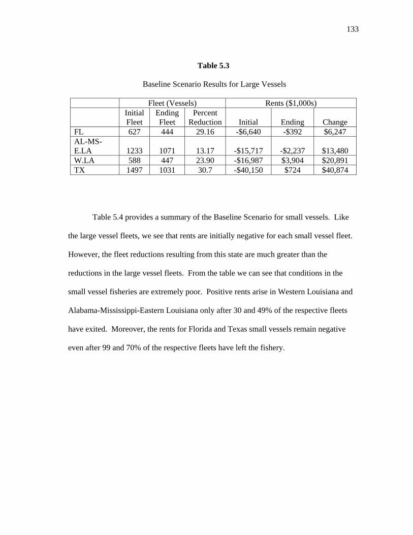
133
Table 5.3
Baseline Scenario Results for Large Vessels
Fleet (Vessels) Rents ($1,000s)
Initial Fleet
Ending Fleet
Percent Reduction Initial Ending Change
FL 627 444 29.16 -$6,640 -$392 $6,247 AL-MS-E.LA 1233 1071 13.17 -$15,717 -$2,237 $13,480 W.LA 588 447 23.90 -$16,987 $3,904 $20,891 TX 1497 1031 30.7 -$40,150 $724 $40,874
Table 5.4 provides a summary of the Baseline Scenario for small vessels. Like
the large vessel fleets, we see that rents are initially negative for each small vessel fleet.
However, the fleet reductions resulting from this state are much greater than the
reductions in the large vessel fleets. From the table we can see that conditions in the
small vessel fisheries are extremely poor. Positive rents arise in Western Louisiana and
Alabama-Mississippi-Eastern Louisiana only after 30 and 49% of the respective fleets
have exited. Moreover, the rents for Florida and Texas small vessels remain negative
even after 99 and 70% of the respective fleets have left the fishery.

134
Table 5.4
Baseline Scenario Results for Small Vessels
Fleet Rents ($1,000s)
Initial
Fleet
Ending
Fleet
Percent
Reduction Initial Ending Change
FL 100% 1.17% 98.83 -$1,185 -$10 $1,175
AL-MS-E.LA 100% 69.91% 30.09 -$3,527 $349 $3,876
W.LA 100% 51.13% 48.87 -$9,869 $2,084 $11,953
TX 100% 28.57% 71.43 -$7,950 -$1,802 $6,148
Table 5.5 shows a summary of the change in landings and catch per unit of effort
(CPUE) under the Baseline Scenario for the large vessel fleets included in the
simulations. Here one can see very large changes in landings for the small vessel fleets
(especially in Florida and Texas), while changes in landings for large vessel fleets are
much less drastic. Conversely, the increases in the CPUE are greater for large vessel
than small because a reduction in small vessel harvests benefits large vessels as shrimp
are able to migrate to offshore waters.

135
Table 5.5
Baseline Landings and Catch per Unit Effort Summary for Large Gulf Vessels
Landings (1,000 lbs) CPUE (lbs/day fished)
Initial Ending %
Change Initial Ending %
Change
FL 7,771.64 6,885.70 -11.4 743.84 937.85 26.08
AL-MS-E.LA 20,224.96 21,572.69 6.66 1,162.56 1,437.03 23.61W.LA 27,259.19 27,783.31 1.92 1,154.56 1,546.18 33.92TX 43,625.14 39,977.23 -8.36 1,066.24 1,410.83 32.32
Scenario 1: Gulfwide SB Program
I now present several policies options that will be compared with the baseline
presented above. The first policy scenario is that of a single gulfwide SB program for
large vessels in addition to the SB program in effect for Texas small vessels. The large
vessel SB program applies to all regions and we assume a budget of $4 million per year.
This budget is chosen arbitrarily, but the qualitative properties of the results would not
change much if the program were scaled up or down depending on the resources
available.
Table 5.6 provides a snapshot of important results of the large vessel SB
program. The program retired 40% of the original capacity, a 20% improvement over
the baseline reductions. Although landings and effort both dropped, the former fell less
than the latter and CPUE rose by 35% over the 10-year simulation horizon. Finally, the

136
fleet rationalization achieved by this program prompted an $88.8 million increase in
fishery rents.
Table 5.6
Gulfwide Sequential Buyback Snapshot (Large Gulf Vessels)
Vessels Landings
(1,000 lbs) Effort (1,000 Days-Fished
CPUE (Lbs/Day-
Fished) Rents
($1,000) Initial 3945 98,880.96 92.37 1,070.49 -$79,493Ending 2402 84,475.94 58.18 1,451.98 $9,375% Change -39.10 -14.57 -37.01 35.64
As a concise measure of the costs and benefits of this SB program the rents
generated by the program are shown in Table 5.7. From the table one can see that in
years 2 and 3 total gulf rents remain negative. In the fourth year the program starts to
payoff in the form of positive fishery rents. The total cost of the program in present
value terms (using a 7% discount rate) is about $28 million. In comparison, the sum of
the present value of total gulf rents in years 2 – 10 is about $28 million. This is a $38
million improvement over the Baseline Scenario, giving a return on investment for the
gulfwide SB program of $1.85 for every dollars spent.
Scenario 2: Gulfwide OTB program
Scenario 2 simulates the effects of a gulfwide OTB program for large vessels in
addition to the SB program for Texas small vessels. This policy scenario differs from

137
Scenario 1 only in the type of auction used for the large vessel buyback. In this section I
present the effects of a OTB program on the Gulf of Mexico’s offshore shrimp fishery.
Table 5.8 provides a summary of results from this simulation. The OTB program
was able to cut the offshore fleet by 61%, increasing fishery rents to $27 million by the
10th year. The fleet reductions pushed CPUE up by 52%. These fleet reductions
represent a substantial improvement over the baseline reduction of 24%. Additionally,
the increase in CPUE is a significant improvement over the 30% increase in CPUE under
the Baseline Scenario.
Table 5.7
Gulfwide Sequential Buyback Annual Rents (7% Discount Rate)
Year Vessels PV Rents ($1,000s)
1 3,945 -$79,493.36 2 3,451 -$30,536.90 3 3,138 -$7,844.48 4 2,829 $837.17 5 2,688 $3,935.23 6 2,629 $4,633.87 7 2,562 $5,004.71 8 2,503 $5,212.96 9 2,453 $5,244.03 10 2,418 $5,099.47 11 2,402
Total (Relative to Baseline)
$38,364.00

138
Table 5.8
Gulfwide One-time Buyback Snapshot (Large Gulf Vessels)
Vessels
Effort (1,000
Days Fished)
Landings
(1,000 lbs) CPUE
Rents
($1,000)
Initial 3,945 92.37 98,880.96 1,070.49 -$79,493
Ending
(year 10) 1,547 35.84 58,574.33 1,634.74 $26,898
% Change -60.79 -61.20 -35.71 52.70
Table 5.9 illustrates the present value of the stream of rents generated by the
gulfwide OTB program. The budget for this program is a single payment of $28 million.
The reductions afforded by the gulfwide OTB program generate over $92 million in total
rents, a huge improvement over the Baseline Scenario, which resulted in a $126 million
loss for the fishery. Relative to the status quo, the gulfwide OTB program has a
rent/cost ratio of $7.79 meaning that for each dollar spent the gulfwide program, there
was a $7.79 increase in rents relative to the the status quo.
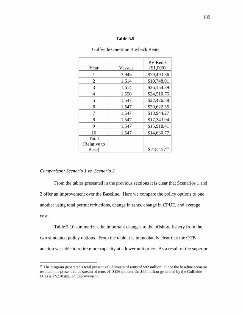
139
Table 5.9
Gulfwide One-time Buyback Rents
Year Vessels PV Rents ($1,000)
1 3,945 -$79,493.362 1,614 $10,748.013 1,614 $26,154.394 1,550 $24,510.755 1,547 $22,476.586 1,547 $20,622.357 1,547 $18,944.278 1,547 $17,343.949 1,547 $15,918.41
10 1,547 $14,630.77Total
(Relative to Base) $218,12756
Comparison: Scenario 1 vs. Scenario 2
From the tables presented in the previous sections it is clear that Scenarios 1 and
2 offer an improvement over the Baseline. Here we compare the policy options to one
another using total permit reductions, change in rents, change in CPUE, and average
cost.
Table 5.10 summarizes the important changes to the offshore fishery from the
two simulated policy options. From the table it is immediately clear that the OTB
auction was able to retire more capacity at a lower unit price. As a result of the superior
56 The program generated a total present value stream of rents of $92 million. Since the baseline scenario resulted in a present value stream of rents of -$126 million, the $92 million generated by the Gulfwide OTB is a $218 million improvement.

140
capacity reductions, the OTB program improved productivity in the fishery by a much
greater margin, pushing catch per unit of effort up by an additional 182.76 pounds per
day fished.
Table 5.10
Gulfwide Sequential and One-time Buyback Auction Comparison
Fleet
Reductions Cost ($1,000)
Avg. Permit
Price
($1,000)
CPUE
Change
(lbs/unit
effort)
SB 1,543 $28,094 $26 381.49
OTB 2,398 $28,094 $12 564.25
Speculative Premium and Permit Prices
In the previous chapter I explored the role of learning in the SB auction and
found that this type of auction leads bidders to attach a speculative premium to their bid.
This speculation, and the dynamic purchasing of the SB auction in general, creates some
interesting differences in prices between the SB and OTB auctions. Table 5.10 shows a
permit price difference between the SB and OTB auctions of around $14,000, when
calculated as total reductions divided by total cost. However, average permit prices by

141
round for the sequential auction shows a much larger discrepancies between the two
auction formats. Table 5.11 shows the average price by round for the SB program.
Table 5.11
Gulfwide Sequential Buyback Auction, Average Price by Round
Year Vessels Reductions
Avg. Price
($1,000s)
1 3,945
2 3,451 494 $8.10
3 3,138 313 $12.78
4 2,829 309 $12.93
5 2,688 141 $28.35
6 2,629 59 $67.73
7 2,562 67 $59.84
8 2,503 59 $68.03
9 2,453 50 $79.97
10 2,418 35 $115.34
11 2,402 16 $252.53
From Table 5.11 it is clear that the SB auction pays a large premium for permits
in later rounds. The bulk of the reductions for this scenario are concentrated in periods

142
during which the fishery is losing money, resulting in low buyout prices and a relatively
low overall average permit price. However, as the auction progresses and capacity is
retired, permit prices begin to rise sharply.
The speculative premium has a compounding effect on permit prices in the SB
program. The average simulated bid in any year is based on the net revenues in the
fishery. As the fishery becomes more profitable, the average bid for the fleet rises. The
speculative component also rises through time reflecting the improved state of the
fishery. So, as vessels are removed from the fishery, we note two effects on the
distribution of bids. The first is that the average simulated bid is rising as a function of
increased profitability. The second is that the speculative component is rising in
conjunction with rising rents. These two effects lead to some extremely high permit
prices in the later years of our simulation.
Regional Simulations
In addition to the two gulfwide scenarios, two regional scenarios were simulated.
In Scenarios 3 and 4, I simulate separate buyback programs for large vessels in each of
the four gulf regions. For comparative purposes the total budget of $4 million annually
is used here just as in the gulfwide programs. However, the budget is allocated to each
region based on its share of total gulf effort in the initial period. Allocation in this
manner is only one of many reasonable ways by which the budget might be divided up
between the regions and I am not advocating this approach over any other. Though
quantitatively the results would vary depending on the allocation rule, I believe that the

143
qualitative features of these results would be reasonably robust to different allocation
rules.
Aggregate Effects
This section compares the regional programs with their gulfwide counterparts.
The main metrics for comparison are fleet reductions, change in CPUE and change in
fishery rents. In the previous discussion of the gulfwide programs, I explored how these
programs affect the gulf as a whole. In this section results will also be aggregated in
order to compare them to gulfwide results.
Table 5.12 summarizes the results of the regional and gulfwide SB programs.
From the table, one can see that the gulfwide SB program categorically dominates its
regional counterpart. Because the gulfwide program seeks out the cheapest permits
throughout the gulf, it is able to achieve much greater fleet reductions than the regional
program. As a result the gulfwide program offers greater increases in both fishery rents
and CPUE.
A particularly interesting fact regarding the comparison of the gulfwide and
regional SB programs is that, although the regional program targets effort, the gulfwide
program actually resulted in a greater effort reduction. This is due in part to the fact that
the region responsible for the greatest portion of total gulf effort (Texas) is also the
region with the cheapest permits initially. So, while the regional SB program allocates
44% of the $4 million budget to buy out permits in Texas, there are so many cheap
permits in Texas that the gulfwide program spends all $4 million in this region in the first
year.
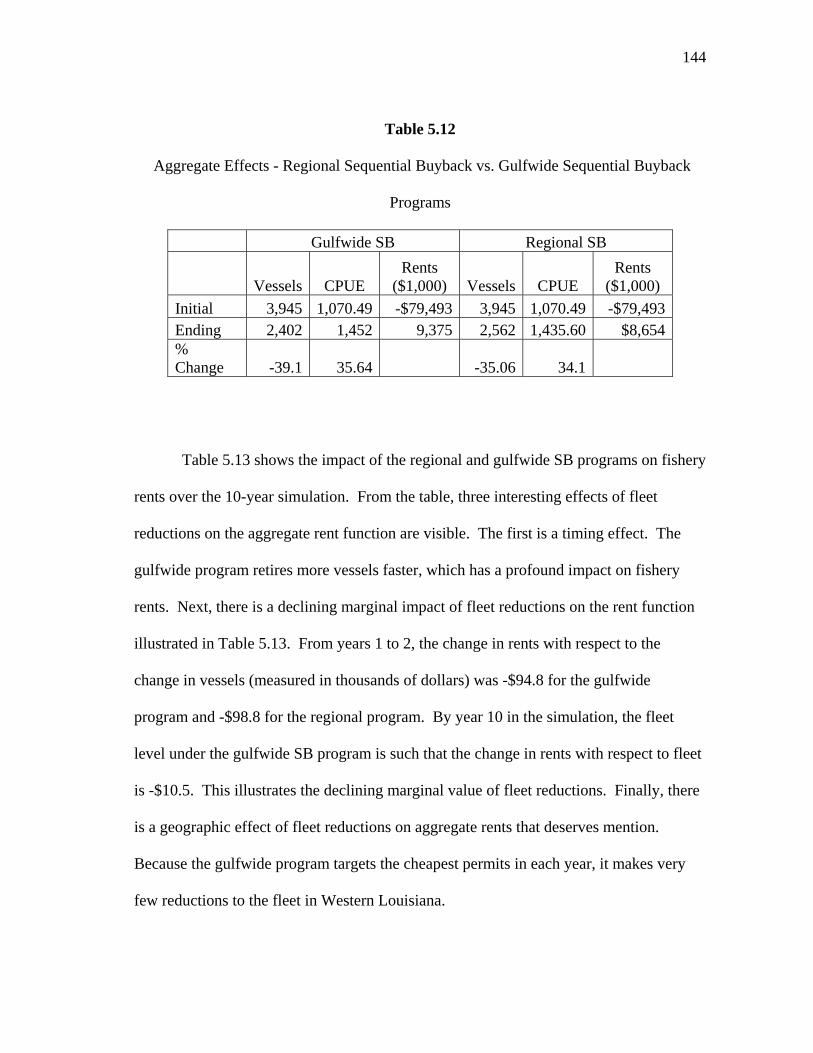
144
Table 5.12
Aggregate Effects - Regional Sequential Buyback vs. Gulfwide Sequential Buyback
Programs
Gulfwide SB Regional SB
Vessels CPUE Rents
($1,000) Vessels CPUE Rents
($1,000)
Initial 3,945 1,070.49 -$79,493 3,945 1,070.49 -$79,493Ending 2,402 1,452 9,375 2,562 1,435.60 $8,654 % Change -39.1 35.64 -35.06 34.1
Table 5.13 shows the impact of the regional and gulfwide SB programs on fishery
rents over the 10-year simulation. From the table, three interesting effects of fleet
reductions on the aggregate rent function are visible. The first is a timing effect. The
gulfwide program retires more vessels faster, which has a profound impact on fishery
rents. Next, there is a declining marginal impact of fleet reductions on the rent function
illustrated in Table 5.13. From years 1 to 2, the change in rents with respect to the
change in vessels (measured in thousands of dollars) was -$94.8 for the gulfwide
program and -$98.8 for the regional program. By year 10 in the simulation, the fleet
level under the gulfwide SB program is such that the change in rents with respect to fleet
is -$10.5. This illustrates the declining marginal value of fleet reductions. Finally, there
is a geographic effect of fleet reductions on aggregate rents that deserves mention.
Because the gulfwide program targets the cheapest permits in each year, it makes very
few reductions to the fleet in Western Louisiana.
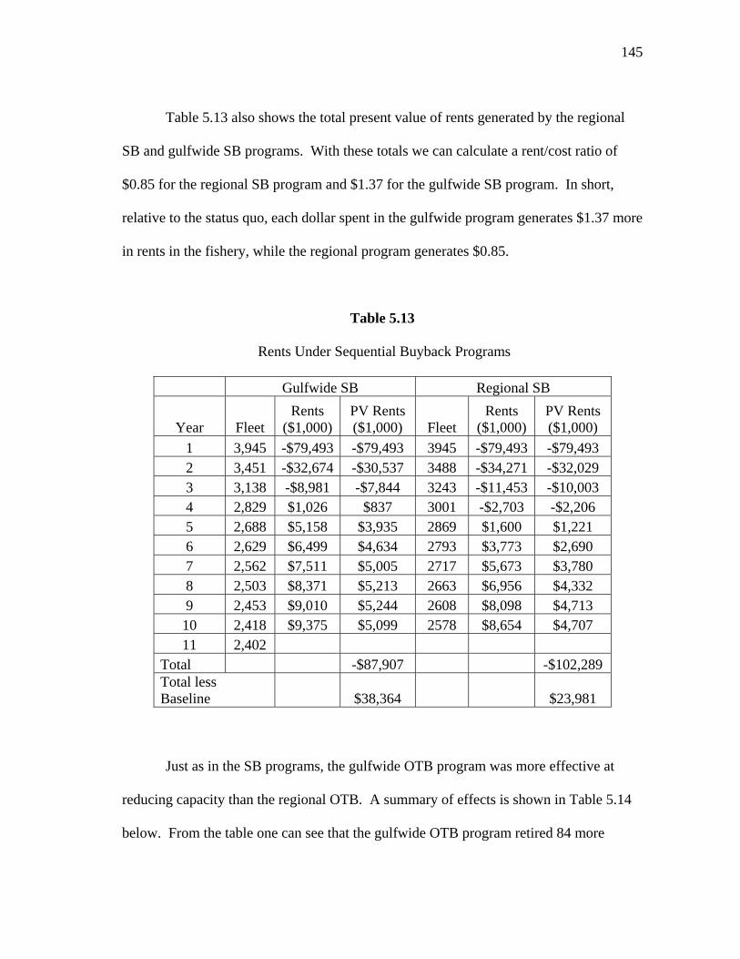
145
Table 5.13 also shows the total present value of rents generated by the regional
SB and gulfwide SB programs. With these totals we can calculate a rent/cost ratio of
$0.85 for the regional SB program and $1.37 for the gulfwide SB program. In short,
relative to the status quo, each dollar spent in the gulfwide program generates $1.37 more
in rents in the fishery, while the regional program generates $0.85.
Table 5.13
Rents Under Sequential Buyback Programs
Gulfwide SB Regional SB
Year Fleet Rents
($1,000) PV Rents ($1,000) Fleet
Rents ($1,000)
PV Rents ($1,000)
1 3,945 -$79,493 -$79,493 3945 -$79,493 -$79,493 2 3,451 -$32,674 -$30,537 3488 -$34,271 -$32,029 3 3,138 -$8,981 -$7,844 3243 -$11,453 -$10,003 4 2,829 $1,026 $837 3001 -$2,703 -$2,206 5 2,688 $5,158 $3,935 2869 $1,600 $1,221 6 2,629 $6,499 $4,634 2793 $3,773 $2,690 7 2,562 $7,511 $5,005 2717 $5,673 $3,780 8 2,503 $8,371 $5,213 2663 $6,956 $4,332 9 2,453 $9,010 $5,244 2608 $8,098 $4,713 10 2,418 $9,375 $5,099 2578 $8,654 $4,707 11 2,402
Total -$87,907 -$102,289 Total less Baseline $38,364 $23,981
Just as in the SB programs, the gulfwide OTB program was more effective at
reducing capacity than the regional OTB. A summary of effects is shown in Table 5.14
below. From the table one can see that the gulfwide OTB program retired 84 more

146
vessels than the regional program. Since the aim of the gulfwide program is to remove
the most vessels per dollar, it is not surprising to see the gulfwide program dominate its
regional counterpart in terms of vessel reductions. Furthermore, because the programs
are operating with identical budgets the greater fleet reduction under the gulfwide
program means that this program also paid a lower average price per vessel. The
gulfwide program paid $11,715 per permit on average, while the regional OTB program
paid an average of $12,138 for each permit that it retired.
The table also shows that the regional OTB program removed more effort than
the gulfwide program. This is not unexpected. Recall that the gulfwide program
removes the cheapest permits without regard for which region they come from. The
regional program distributes the total budget across the regions based on each region’s
share of total gulf effort in the initial period. Hence the regional OTB program directs
larger portions of the total budget to high effort regions. Although the gulfwide program
retires more total vessels, the regional OTB program retires more from Texas and
Western Louisiana. These two regions collectively are responsible for 70% of total gulf
effort in the initial period. Thus, it is not surprising to see greater effort reductions under
the regional OTB program.

147
Table 5.14
Aggregate Effects – Regional One-time Buyback vs. Gulfwide One-Time Buyback Programs
Gulfwide OTB Regional OTB
Vessels
Effort (1,000 days
fished)
Landings (1,000
lbs)
CPUE (lbs/day fished) Vessels
Effort (1,000 days
fished)
Landings (1,000
lbs)
CPUE (lbs/day fished)
Initial 3,945 92.37 98,880.96 1,070.49 3,945 92.37 98,880.96 1,070.49
Ending 1,547 35.83 58,574.33 1,634.74 1,631 35.00 56,882.34 1,625.35
% Change -60.79 -61.21 -40.76 52.71 -58.67 -62.11 -42.47 51.83
147
148
The superior effort reductions under the regional program also mean that the
regional OTB program paid slightly less on average per unit of effort. The regional
program paid an average of $489 per unit of effort retired, while the gulfwide program
paid an average of $496 for each unit of effort it retired.
It is interesting to note that, although the regional OTB program removed more
effort than the gulfwide program, the gulfwide OTB actually resulted in a greater
increase in productivity (as measured by CPUE). The gulfwide program retired much
more effort from Florida than the regional program. Because FL was initially the least
productive region, the gulfwide program had a greater impact on aggregate productivity
in the gulf than the regional OTB program.
Finally, from Table 5.15 below, one can see that the gulfwide program was able
to generate more rents in the gulf over our 10-year simulation than the regional OTB
program. Relative to the Baseline Scenario, the gulfwide program was able to generate
$7.76 in rents for each dollar spent, while the regional program produced $7.66 in rents
for each dollar spent.
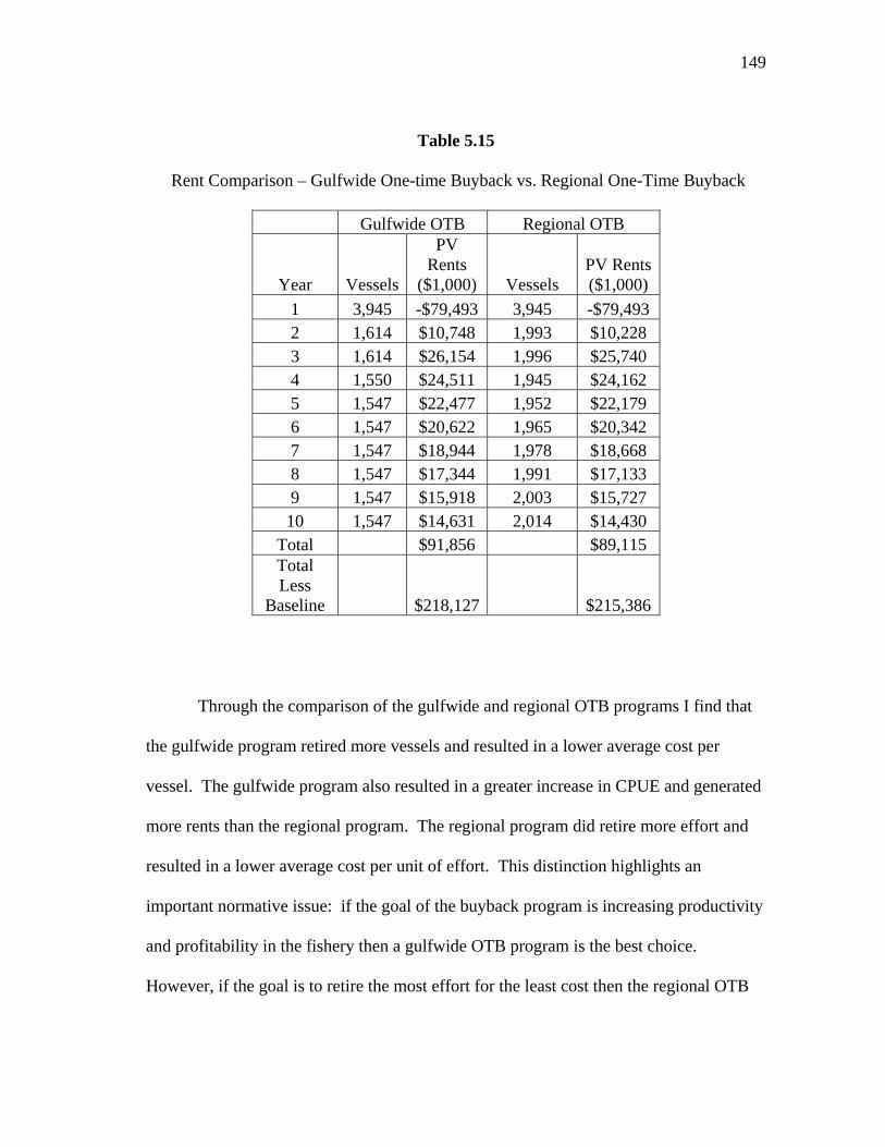
149
Table 5.15
Rent Comparison – Gulfwide One-time Buyback vs. Regional One-Time Buyback
Gulfwide OTB Regional OTB
Year Vessels
PV Rents
($1,000) Vessels PV Rents ($1,000)
1 3,945 -$79,493 3,945 -$79,493 2 1,614 $10,748 1,993 $10,228 3 1,614 $26,154 1,996 $25,740 4 1,550 $24,511 1,945 $24,162 5 1,547 $22,477 1,952 $22,179 6 1,547 $20,622 1,965 $20,342 7 1,547 $18,944 1,978 $18,668 8 1,547 $17,344 1,991 $17,133 9 1,547 $15,918 2,003 $15,727 10 1,547 $14,631 2,014 $14,430
Total $91,856 $89,115 Total Less
Baseline $218,127 $215,386
Through the comparison of the gulfwide and regional OTB programs I find that
the gulfwide program retired more vessels and resulted in a lower average cost per
vessel. The gulfwide program also resulted in a greater increase in CPUE and generated
more rents than the regional program. The regional program did retire more effort and
resulted in a lower average cost per unit of effort. This distinction highlights an
important normative issue: if the goal of the buyback program is increasing productivity
and profitability in the fishery then a gulfwide OTB program is the best choice.
However, if the goal is to retire the most effort for the least cost then the regional OTB
150
program would be preferred. However, I find that with the budget distributed based on
the initial levels of effort, the difference between the regional and gulf-wide OTB
programs is relatively slight. In contrast, under a SB program, the regional program is
much less effective than the gulf-wide program.
Regional Effects
The analysis in this chapter has shown that, among SB programs, a gulfwide
program retires more effort at a lower unit cost, generates more rents for the fishery, and
increases productivity by a greater margin than a regional SB program. However,
among OTB programs, the relative ranking depends on the preferred evaluation criteria.
Up to this point I have focused the evaluation on the aggregate benefits of each
program without regard for how these benefits are distributed. In this section I explore
program impacts by region and discuss distributional implications.
Expenditures
Table 5.16 shows the amount spent in each region by each of the four programs.
It is evident that the gulfwide SB program spends considerably more in regions 2 and 4
than in regions 1 and 3. Interestingly, the gulfwide SB program spends very little money
at all in Western Louisiana, Region 3. By design, the regional programs spend
according to each region’s initial effort level so there are no real surprises in the
spending patterns for the regional SB and OTB programs. However, in the gulfwide
OTB program one again sees that the program spends a disproportionate amount in the
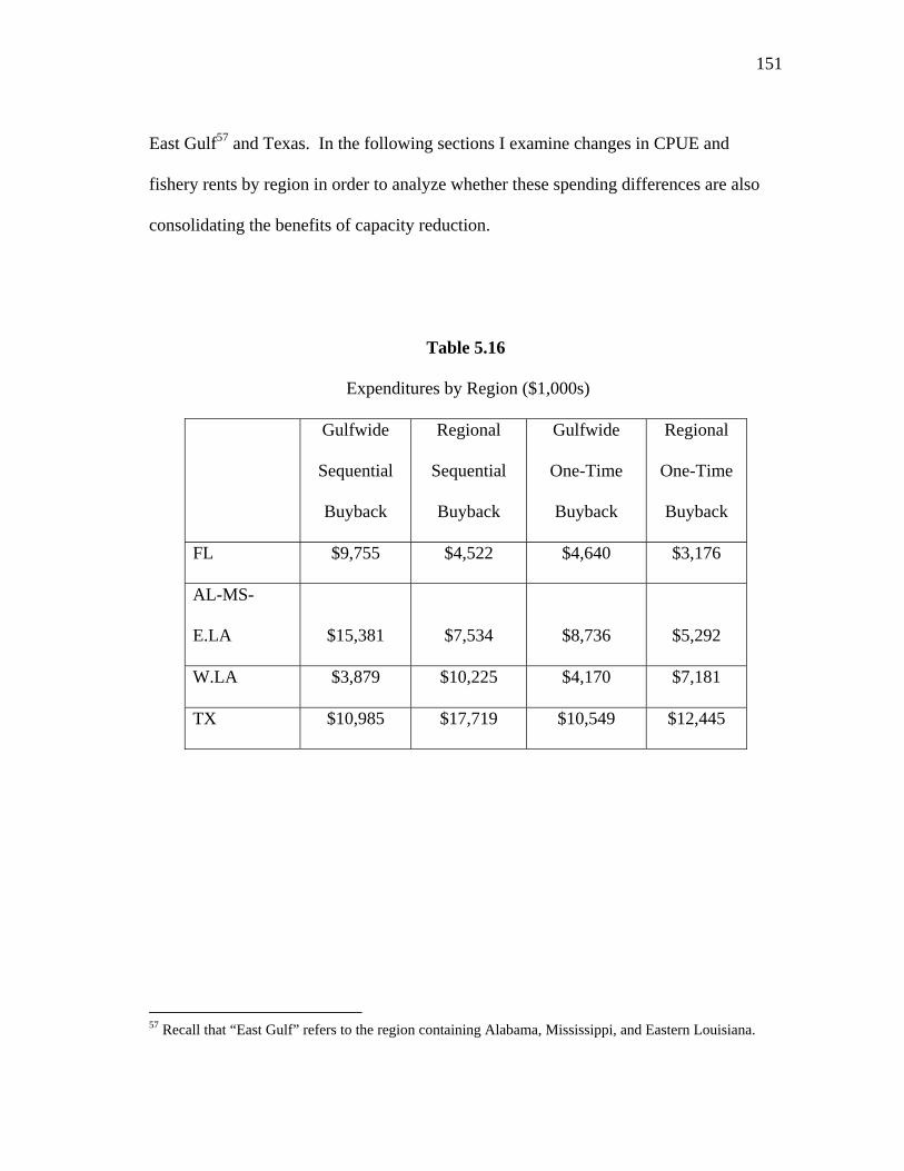
151
East Gulf57 and Texas. In the following sections I examine changes in CPUE and
fishery rents by region in order to analyze whether these spending differences are also
consolidating the benefits of capacity reduction.
Table 5.16
Expenditures by Region ($1,000s)
Gulfwide
Sequential
Buyback
Regional
Sequential
Buyback
Gulfwide
One-Time
Buyback
Regional
One-Time
Buyback
FL $9,755 $4,522 $4,640 $3,176
AL-MS-
E.LA $15,381 $7,534 $8,736 $5,292
W.LA $3,879 $10,225 $4,170 $7,181
TX $10,985 $17,719 $10,549 $12,445
57 Recall that “East Gulf” refers to the region containing Alabama, Mississippi, and Eastern Louisiana.

152
CPUE Changes by Region
One of the potential benefits of removing vessels from the fisheries is improved
productivity as measured by CPUE. Table 5.17 shows the percent change in CPUE in
each region, under each of the four programs. Previously, it was shown that the
gulfwide programs spend a disproportionate amount of money in Texas and the East
Gulf . From the table below one can see that, in Texas at least, this appears to be money
well spent. Texas experiences the greatest increase in CPUE under all four of the
programs.
Interestingly, the percentage increase in CPUE in the East Gulf is low relative to
the other regions. East Gulf has the lowest CPUE increase under all programs
considered here. Focusing on the gulfwide SB program, one can see that expenditures
for East Gulf are much higher than for any other region yet the productivity increase
there is smaller than in any other region. The CPUE change is, in fact, the cause of the
high expenditure level. Because productivity stays relatively low in East Gulf, permit
prices remain cheap compared to other regions. The gulfwide SB program purchases
more permits from East Gulf than Florida and Western Louisiana combined.

153
Table 5.17
Change in Catch per Unit Effort by Region (% Change)
Gulfwide SB Regional SB
Gulfwide
OTB
Regional
OTB
FL 41.49 30.10 57.38 48.23
AL-MS-
E.LA 28.98 29.30 44.31 43.02
W.LA 33.50 38.20 52.17 55.44
TX 35.36 33.93 56.63 60.27
Although there are some large differences in spending by region among the four
simulated programs, Table 5.17 shows that the changes in productivity across regions is
fairly even within each program. The largest spread (as measured by the maximum
increase less the minimum increase) in productivity increase is 17.25% under the
regional OTB program. And even under this program the lowest productivity change
was a 43.02% increase in CPUE.
Rents
To determine how rents are distributed across the various regions, I examine the
rents generated by each program and each region’s share of that total. Table 5.18 shows

154
the 10-year present value total of rents above the baseline58 generated by each program
for each region.
From Table 5.18 it appears that the monetary benefits of each program are
heavily concentrated in East Gulf and Texas. In both regional programs as well as the
gulfwide OTB program these two regions collect over 75% of the aggregate benefits.
Moreover, Texas collects over 40% of the aggregate benefits in all programs with the
exception of the Regional SB program. Given the amount of money spent in Texas, it is
not surprising to see benefits concentrated in this region.
Table 5.18
Total Rents Above Baseline (Present Value, $1,000)
Gulfwide SB Regional SB
Gulfwide
OTB
Regional
OTB
FL $4,462 -$216 $27,350 $23,651
AL-MS-
E.LA $24,448 $11,085 $48,876 $53,581
W.LA -$38,048 $5,736 $27,224 $18,871
TX $29,243 $7,377 $114,676 $88,036
Aggregate $20,105 $23,981 $218,127 $184,139
Max – Min $67,291 $11,301 $87,452 $69,165
58 To get these figures I sum the present value of rents in each region under each program and subtract the present value sum of rents under the baseline scenario.

155
Unlike the increase in CPUE, there is a very inequitable distribution of rents
among the regions, under all four programs. From the table above one can see that the
most even distribution of rents, as measured by the spread between the largest and
smallest gain, was provided by the regional SB program. However, this program also
generated substantially fewer rents than any other. It is also interesting to note that the
gulfwide OTB program generated more aggregate rents than the regional OTB program
and these benefits were more equitably distributed.
From Table 5.18 above one can see that Western Louisiana is actually worse off
under the gulfwide SB program then under the status quo. This is a unique result and it
is worth diverting briefly from the equity discussion to provide an explanation. One
assumption of the model is that owners will not voluntarily leave the fishery when a
buyback is in place. In Western Louisiana, like each of the other regions, rents are
initially predicted to be negative. However, without any capacity reduction, positive
rents are generated by the 3rd year. Because the gulfwide SB program spends so little
money in Western Louisiana, there are few changes in the fleet. Under the Baseline
Scenario, vessels exit the fishery in the presence of negative rents and this eventually
leads to increasing rents in Western Louisiana. While this result follows from a
modeling assumption that boats will not voluntarily leave the fishery if a buyback
program is in place, this assumption may be reasonable. If the government announces
that it will be paying for permits, those assets take on an option value that creates an
incentive for the fishermen to keep them active even if normal fishery economics is
working against them.

156
Texas Inshore Buyback
From Table 5.18 one immediately notes extraordinary rent levels generated in
Texas by both OTB programs. With total rents of $114 million under the gulfwide OTB
and $88 million under the regional OTB, Texas is far and away the most profitable
region in the gulf. An important factor contributing to this profitability is the presence
of the state run buyback program in the inshore fishery. The inshore buyback program
in Texas removes vessels from the bay system, allowing more shrimp to migrate to
offshore areas.
In all regions total landings and total revenues tend to fall as vessels are removed
from the fisheries. This means that the decline in total landings resulting from fleet
reduction is not being offset by an equal increase in the value of landings. The result of
this pattern for the present analysis is that declining landings have a negative effect on
fishery rents. In Texas, fleet reductions have a smaller effect on total landings than in
other regions.

157
To illustrate the impact of buyouts on total landings I show the year-by-year
change in landings with respect to changes in effort in Table 5.19. Here I focus on the
regional SB Program because it is the only program which led to reductions in every
year. Looking at the last five years of the simulation, one can see that the effect of effort
reductions on landings was considerably smaller in Texas than in either Western
Louisiana or the East Gulf region. During this time large vessel effort was being
removed from all fisheries but, since Texas was also removing effort from its inshore
fishery concurrently, gulf landings were impacted to a smaller degree.
The comparison between East Gulf and Texas is particularly informative because
the CPUE is very similar in these two regions. In Table 5.20 the CPUE was clearly
higher in East Gulf than in TX, but only by an average of about 66 lbs/day fished, per
year. Looking at the change in landings with respect to changes in effort, one can see a
much larger difference: removing 1 unit of effort from East Gulf resulted in an average
loss of 750 lbs, while a 1 unit effort reduction in TX costs an average of 786 lbs. From
this table it is clear that, while East Gulf was slightly more productive than TX, the
difference in the impact of effort reductions on landings between these two regions was
well out of proportion to the productivity difference.

158
Table 5.19
Regional Sequential Buyback Program’s Change in Landings with Respect to
Change in Effort (Change in lbs/ Change in Days-Fished)
Year FL
AL-MS-
E.LA W.LA TX
1
2 202.79 -1,091.63 -217.95 214.67
3 151.48 70.41 -191.19 167.52
4 285.94 958.89 758.54 902.11
5 377.22 1,074.94 941.60 886.94
6 304.56 1,072.38 1,630.51 1,027.26
7 458.68 1,060.72 1,408.58 865.45
8 470.41 1,194.99 1,626.00 1,010.76
9 488.78 1,118.84 1,480.72 950.33
10 463.38 1,290.54 1,968.09 1,047.67

159
Table 5.20
Landings and Effort Comparison for Regions 2 and 4
AL-MS-E.LA TX
Year
Effort (days
fished)
CPUE (lbs/day fished)
Change in Landings/ Change in
Effort
Effort (days
fished)
CPUE (lbs/days fished)
Change in Landings/ Change in
Effort
1 17,397 1,162.56 40,915 1,066.24 2 16,197 1,329.56 -1,091.63 34,936 1,211.98 214.673 15,089 1,422.02 70.41 32,126 1,303.33 167.524 14,060 1,455.92 958.89 28,772 1,350.10 902.115 13,439 1,473.52 1,074.94 27,334 1,374.47 886.946 13,190 1,481.10 1,072.38 26,175 1,389.84 1,027.267 12,918 1,489.95 1,060.72 25,504 1,403.64 865.458 12,684 1,495.39 1,194.99 24,909 1,413.03 1,010.769 12,491 1,501.21 1,118.84 24,397 1,422.74 950.3310 12,374 1,503.20 1,290.54 24,058 1,428.02 1,047.67
Average 750.01 785.86
The primary reason that Texas is able to remove vessels from the offshore fishery
with less impact on landings (as other regions) is because of effort reductions in the
inshore fishery. From Table 5.21 below, one can see that initially all of the inshore
fisheries experience a sharp decrease in landings. This is because the inshore fisheries
are unprofitable at the start so many of the vessels exit in the first two years. However,
with open access, as profitability improves effort begins to move back into the fisheries
and landings increase. In East Gulf and Western Louisiana landings begin to increase
steadily after the 3rd year. Meanwhile, landings in the Texas inshore fishery fall by an
average of just over 487,000 lbs per year throughout the 10-year simulation.

160
Table 5.21
Landings and Effort for Inshore Fisheries Under Regional Sequential Buyback
FL AL-MS-E.LA W.LA TX
Year
Effort (Days
Fished)
Change in
Landings (‘000 lbs)
Effort (Days
Fished)
Change in
Landings (‘000 lbs)
Effort (Days
Fished)
Change in Landings (‘000 lbs)
Effort (Days
Fished)
Change in
Landings (‘000 lbs)
1 1,604 9,921 32,586 12,466
2 849 -458.11 7,539 -1,149.16 14,352 -12,519.24 11,839 -6.813 475 -235.47 6,810 -498.97 14,580 498.67 11,808 115.94 281 -127.32 6,816 70.61 14,886 347.88 11,769 49.555 172 -72.96 6,846 55.47 15,206 318.05 11,742 22.166 109 -43.76 6,884 43.37 15,529 302.31 11,722 11.557 70 -27.11 6,924 53.98 15,850 347.66 11,699 10.678 45 -17.11 6,967 44.78 16,180 309.52 11,675 1.79 30 -10.96 7,010 49.37 16,510 337.15 11,652 3.810 20 -7.12 7,055 39.71 16,844 303.92 11,633 -2.51
160

161
Here I have presented several statistics on landings and effort in order to analyze
the impact of the inshore buyback in Texas on offshore rents. I have shown that the
impact on landings of a one unit effort reduction in Texas is small relative to the other
regions. This is due, in large part, to the presence of the inshore buyback program which
cuts landings from the bay system by an average of close to half a million pounds per
year. By reducing inshore effort, the small vessel buyback program helps improve the
profitability of the offshore fishery in Texas.
Program Evaluation Summary
There were two main goals for the analysis provided in this chapter. The first
was to assess the cost and effectiveness of SB programs relative to OTB programs. And
the second was to compare a policy of multiple regional markets for buyback with a
single gulfwide market for both SB and OTB programs. Table 5.22 provides a
composite of evaluation criteria.

162
Table 5.22
Four Program Ranking – Rank in Parentheses
Gulfwide Sequential Buyback
Regional Sequential Buybakc
Gulfwide One-Time
Buyback
Regional One-Time
Buyback
Reductions
Vessels 1,543
(3) 1,383
(4) 2,398
(1) 2,314
(2)
Effort 34,190
(3) 32,773
(4) 56,539
(2) 57,373
(1)
Productivity
CPUE Increase 381.49
(3) 365.11
(4) 654.25
(1) 554.86
(2)
Efficiency
Cost per Permit $26,930
(3) $28,918
(4) $11,714
(1) $12,138
(2)
Cost per Unit of Effort
$1,169 (3)
$1,220 (4)
$513 (1)
$668 (2)
Net Profitability
Present Value of Rents
$38,364 (3)
$23,981 (4)
$218,127 (1)
$215,386 (2)
Benefits/Cost $1.37
(3) $0.85
(4) $7.76
(1) $7.66
(2)
Equity (Rank Only)59 Equity in Productivity 3 1 2 4
Equity in Rents 2 1 3 4
Average Rank 2.89 3.33 1.44 2.11
59 The equity measures used here are simply the difference between the region of greatest gain and the region of least gain for each program. Equity in productivity for example is determined by the difference between the region of greatest CPUE increase and the region of least CPUE increase under each program.

163
It is clear from Table 5.22 that the OTB programs were able to retire more effort
at a much lower cost than their SB counterparts. These reductions resulted in greater
productivity increases and greater increases in fishery rents. The table also shows that
the regional programs offered little advantage over the gulfwide programs. The regional
SB was almost categorically dominated by its gulfwide counterpart (ranking below the
gulfwide SB program in 7 out of 9 measures). And, while the regional OTB program
retired more effort at a lower unit cost then its gulfwide counterpart, the gulfwide OTB
program generated superior rents resulting in a more favorable rent/cost ratio for the
program.
The 2nd Best Policy
In this chapter I have shown that, when offered the choice between buying back
permits sequentially over time or spending the present value of a stream of sequential
payments to buyback permits in a single year, more effort can be reduced from the
fishery with the single upfront payment. However, a prominent advantage to a
sequential buyout is that it does not require a large initial investment. Because of this
very practical advantage, SB programs may still find a place in the regulator’s toolkit.
Although, on the basis of rents, productivity increases and permit reductions, an OTB
program would be preferred, for managers who chose the SB program for capacity
reduction, understanding how capacity reductions influence fleet rents can help
regulators run an SB program more effectively.
Removing vessels from the fleet will have biological and economic impacts on
the fishery. However, many of these effects (such as an increase in abundance or
164
increase in size of shrimp landed) will relate back to the rent function. Fishery rents are
a compact measure of program success which captures many biological and economic
relationships. In the previous sections I have discussed how each of the simulated
programs affects the rent function. In this section I briefly discuss how vessel reductions
in general impact fishery rents and how this information could be used to improve the
efficacy of an SB program.
In GBFSM, vessel reductions influence rents mainly through their effect on
landings and the cost structure. Landings affect revenues which, in turn, affect rents
while cost has a more direct effect on rents.
Conceptually, one expects that inefficient producers will be the first to sell back
their permits. The immediate effect of this exit will be to reduce aggregate cost relative
to revenues and increase rents. However, as profitability in the fishery increases
remaining vessels have an incentive to expand operations, which tends to eat away at
rents. Because GBFSM is a homogeneous fleet model, fleet costs fall in direct
proportion to vessel reductions. Furthermore, effort in the fishery is assumed to be
directly related to the number of vessels. Therefore, the simulation model is not capable
of analyzing these cost issues.
The biological submodel included in GBFSM does, however, allow us to analyze
the behavior of landings under buyback regimes. The immediate impact of vessel
reductions will be to reduce total landings. But over the longer term, we cannot say a
priori whether total landings will rise or fall with vessel reductions. If the stock is
overfished initially, and if overfishing is severe, then it is possible to see total landings

165
increase over the longer term. Removing vessels, and hence fishing pressure, may
improve recruitment, leading to increased abundance in later years. Given the annual
nature of shrimp fisheries, however, what the simulations actually show are total
landings decreasing with vessel reductions.
The effect of changes in landings on fishery rents comes through the revenue
function. Revenues are made up of total landings and value of landings. Declining total
landings have a negative impact on revenues. However, this effect may be reduced by
the size effect. As total shrimp landings decrease, the expectation is that value per
pound will rise as shrimp are allowed to reach a larger size before harvest. While the
impact of landings on revenue and therefore rents may be predicted a priori (with
sufficient information regarding the yield curve), it cannot be know. What the
simulations show is that total revenues are decreasing with vessel reductions, meaning
that the positive impact on the revenue function of value increase is dominated by the
negative impact of volume decrease.
Here I have discussed how vessel reductions relate to fishery rents through their
effects on the cost and revenue functions. Focusing on the SB programs, one can see the
impact of vessel reductions on rents through time. In simple economic terms one can
think of the additional rents generated through vessel reductions as the marginal benefit
of the program. By examining the last purchased in each year it is also possible to
calculate the marginal cost – the cost required to purchase one additional vessel. These
two quantities are shown below in Table 5.23.

166
Table 5.23
Marginal Benefit and Cost to Purchase One Additional Vessel for Gulfwide Sequential
Buyback Program
Year
Vessel
Reduction
Marginal
Benefit Marginal Cost
1 $8,100
2 494 $94,810 $8,750
3 313 $75,680 $10,330
4 309 $32,340 $13,470
5 141 $29,290 $58,460
6 59 $22,700 $230,850
7 67 $15,130 $261,090
8 59 $14,630 $259,270
9 50 $12,780 $279,390
10 35 $10,520 $493,840

167
The table shows that vessel reductions initially have a very large payoff since
marginal benefits greatly exceed marginal cost. However, this payoff declines
substantially as more and more vessels are removed. By year five the marginal cost
exceeds the marginal benefit by a factor of almost four and by the 10th year buying an
additional permit under the gulfwide SB program only generates an additional $10,520
but costs almost a half million dollars.
In Table 5.24 below, I present the change in rents per dollar spent in each year of
the sequential auction. From the table one can see that by the 6th year the additional
rents generated by the programs were less than the amount spent and therefore the
change in rents per $ spent falls below 1 in these years. Furthermore, by the final year of
the simulation, the change in rents per dollar spent drops to a dismal $0.09 for the
gulfwide SB and $0.14 for the regional SB.
Although not as effective as OTB programs, SB programs offer managers an
affordable alternative to expensive one-time programs. Managers would have the option
of ending the program if they see that the marginal costs are greater than the marginal

168
Table 5.24
Change in Rents per Dollar Spent for Sequential Buyback Programs
Year Gulfwide SB Regional SB
1
2 $11.70 $11.31
3 $5.92 $5.70
4 $2.50 $2.19
5 $1.03 $1.08
6 $0.34 $0.54
7 $0.25 $0.48
8 $0.22 $0.32
9 $0.16 $0.29
10 $0.09 $0.14
benefits. In this section I have shown that the marginal benefit of vessel reductions
declines over time and as such the SB programs generate very few benefits per dollar
spent in the later years. One relatively simple rule which may increase the cost
effectiveness of the SB programs substantially would be to place a cap on permit price.
Managers with a thorough understanding of the economics of the fishery will be better
169
able to place this cap appropriately, though even for the most experienced and
knowledgeable managers, the difficulty of the task is significant.
In sum, SB programs, although they do not compare favorably to OTBs based on
the criteria presented in this chapter, may provide managers with a more cautious
approach to buying back permits. In a highly variable industry, such as shrimping in the
Gulf of Mexico, the idea of “optimal” reductions will likely change drastically from one
year to the next. A SB program would allow regulators to update their purchasing goals
and criteria as economic conditions in the fishery change or as new information becomes
available. In this section I have presented some evidence on marginal benefits and
marginal costs of reductions. Managers who prefer a cautious approach to reductions in
capital may favor a SB program, the analysis presented in this section may help
rationalize the use of a sequential program.
Summary of Simulation Work
In this chapter I have shown that OTB programs, by virtue of avoiding the
speculative premium, retire more effort faster, and at a lower cost, then SB programs.
This produces biological and economic benefits for the shrimp fisheries in the Gulf of
Mexico under which are far superior to those generated by SB programs. I have also
shown that single market buyback programs perform better in the Gulf of Mexico then
programs using multiple regional markets.

170
CHAPTER VI
SUMMARY AND CONCLUSIONS
This dissertation has provided a thorough analysis of the cost and effectiveness
of sequential buyback auctions relative to one-time buyback auctions for renewable
resource management. For this study I have developed an empirical model of bidding
behavior in a sequential license buyback auction. I used data from the Texas Inshore
Shrimp License Buyback Program – a long running sequential buyback auction – to
estimate parameters of this model. With these parameters, a model was developed to
simulate two hypothetical buyback policies: a sequential license buyback program for
offshore shrimp vessels in the Gulf of Mexico and a one-time buyback program for
offshore shrimp vessels in the Gulf of Mexico. Simulating two alternative programs for
capacity reduction in the same fishery allowed for the comparison of the auction
formats.
In Chapter II, a literature review on auctions and bidding was provided to
establish some background for our study. The literature on auctions and bidding both
from traditional economics and environmental economics is very well developed.
Furthermore, the game theoretic foundations of bidding, and in particular the elements of
strategy involving one bidder against another, have been explored at length in the
auction theory literature. However, the topic of strategy as it applies to sequential
auctions has received notably less attention. A contribution of this dissertation is that it
provides an in depth study of bidding strategy when participants are allowed to learn
about the buyer’s value over the course of a repeated game.
171
Chapter III gave a statistical summary of the Texas Inshore Shrimp License
Buyback Program. The objective in this chapter was to provide the basic motivation for
our formal dynamic econometric model. In Chapter III I showed that over half of all
participants in the buyback auction placed bids in more than one round. I also showed
that the distribution of all bids placed in the auction becomes progressively tighter as the
auction progresses. In the first round of the auctions bids are distributed very diffusely
but by the fourteenth round we see bids clustered very tightly around the average license
price. This suggests that bidders are learning about the agency’s willingness to pay as
the auction progresses and using this informing in submitting bids.
In Chapter IV I presented an econometric model used to estimate parameters of
the fisherman’s bidding function in a sequential auction. The primary objective of this
chapter was to estimate the parameters of the fisherman’s underlying benefit function
and to distinguish this from the speculative premium induced by the sequential auction
format. This was done by first setting up a dynamic programming algorithm to solve the
dynamic optimization problem characterizing the fisherman’s decision problem. The DP
problem was then nested inside of an estimation algorithm which searched for optimal
parameters by minimizing the sum of squared errors between actual and predicted bids.
The results of the estimation showed a speculative component which was initially very
high and volatile over the early years of the auction but which leveled out over the later
years. The estimates suggest an initial speculative premium equal to 3.6 times individual
benefits in the first round of the auction and a shape decline to 1.3 times individual
benefits for the second round. There was very little change in the speculative premium

172
after the 10th round as it stayed consistently between 1.8 and 1.9 times individual
benefits.
In addition to providing the estimates needed for effective policy comparison,
Chapter IV makes some important methodological contributions. First, I use a Bayesian
updating algorithm to introduce learning to our dynamic optimization problem. This
represents a contribution in the modeling of bidding under a sequential auction where
information transmission is an important part of the decision problem. Next, this
analysis considered a control variable (bid amount) that is continuous. This marks an
important departure from previous exercises in estimation of dynamic decision problems
(Rust 1988, Miranda and Schnitkey 1995, and Provencher and Bishop 1997) which all
use a binary decision variable.
The main objective of Chapter V was to use a simulation model to compare the
cost and effectiveness of a sequential license buyback program relative to a one-time
buyback program for capacity reduction in the Gulf of Mexico shrimp fishery. In this
chapter I showed that the sequential buyback program, because of the speculative
premium induced by this particular auction format, retires substantially less effort per
dollar spent then the one-time buyback program. In this chapter I found that, if faced
with the choice of spending a buyout budget over several years or spending the present
value of a sequential stream of payments in a single year, fisheries managers would
usually be better off choosing the one-time auction format.
As is often the case with complex estimation, it was necessary throughout this
dissertation to make some simplifications. Although these were deemed necessary and

173
defensible, future work in this area should concentrate on refining the estimation
algorithm. In particular, there may be room to increase the precision of the point
estimates by refining the grid search boundaries. The grid search method was deemed
the most appropriate algorithm to achieve maximization given the heavy non-linearities
in the objective function. However, future research may be able to add some precision
to the estimates.
In addition to further refinements in the grid search, a second suggestion for
future work is to concentrate on the structure that was imposed on the benefit function.
Currently, the benefit function contains the explanatory variables price and vessel length.
There was some evidence presented in Chapter III that license holder age should also be
incorporated into the fisherman’s benefit function. Because of the computational
intensity of the estimation algorithm, it was not possible to add another variable to the
structure. However, future research that strives to improve the efficiency of estimation
may provide an important extension to this work by making it possible to add more
explanatory variables to the R function that estimates the value of a fishing license.
It should also be reiterated that the simulation results, presented in the previous
chapter, were based on an earlier version of the model. This model was parameterized
using the best data available at the time. Since then, data improvements have led to a re-
parameterization of the simulation model and updated results can be found in Woodward
and Griffin (2008). It should be made clear however, that the updated model bears no
qualitative differences from the model used in this analysis. While the results derived
from the final simulation model differ quantitatively from those presented in Chapter V,

174
the conclusions presented in this dissertation regarding the performance of sequential
auctions relative to one-time buyback auctions remain intact.
175
NOMENCLATURE
BSAI Bering Sea Aluetian Islands
CPUE Catch per Unit of Effort
DGP Data Generating Process
DP Dynamic Programming
EEZ Exclusive Economic Zone
FAO Food and Agriculture Organization of the United Nations
GBFSM General Bioeconomic Fisheries Simulation Model
MAE Mean Absolute Error
Magnuson-Stevens Magnuson-Steven Fisheries Conservation and Management Act
ML Maximum Likelihood
NMFS National Marine Fisheries Service
OLS Ordinary Least Squares
OTB One-time buyback
PV Present Value
RFP Relative Fishing Power
SB Sequential buyback
SSE Sum of Squared Errors
TPWD Texas Parks and Wildlife Department
176
REFERENCES
Ashenfelter, O. 1989. How Auctions Work for Wine and Art. Journal of Economic
Perspectives. 3(3): 23-36. Curtis, R and D. Squires. 2007. Fisheries Buybacks. Ames, IA: Blackwell. Deltas, G. and G. Kosmopoulou. 2004. Catalogue vs Order-Of-Sale Effects in Sequential Auctions: Theory and Evidence from a Rare Book Sale. The Economic Journal, 114(492): 28-58.
Funk, R.D, W.L Griffin, J.W Mjelde, and J.M Ward. 2003. A Simulation Model of License Buyback in the Texas Bay Shrimp Fishery. Marine Resource Economics 18(1): 33 – 53.
Ginsburgh, V. 1998. Absentee Bidders and the Declining Price Anomaly in Wine Auctions. Journal of Political Economy, 106(6): 1302-1319.
Ginsburgh, V. and J.C van Ours. 2007. On Organizing a Sequential Auction: Results from a Natural Experiment by Christie’s. Oxford Economic Papers, 59(1): 1–15.
Grant, W.E and W.L Griffin. 1979. A Bioeconomic Model of the Gulf of Mexico Shrimp Fishery. Transactions of the American Fisheries Society 108(1): 1 – 13.
Grant, W.E, K.G Isakson, and W.L. Griffin. 1981. A General Bioeconomic Simulation Model for Annual-Crop Marine Fisheries. Ecological Modeling 3(3): 195 – 219.
Greene, W.H. 2003. Econometric Analysis. Upper Saddle River, NJ: Prentice Hall. Griffin, W.L., A.K. Shah, and J.M. Nance. 1997. Estimation of Standardized Effort in
the Heterogeneous Gulf of Mexico Shrimp Fleet. Marine Fisheries Review. 59(3): 23-33.
Grooves, T. and D. Squires. 2007. Lessons from Fisheries Buybacks. Fisheries
Buybacks, Curtis, R and D. Squires, eds., pp. 15-55. Ames, IA: Blackwell. Haby, M.G., R.J. Miget, L.L. Falconer, and G.L. Graham. 2002. A Review of Current
Conditions in The Texas Shrimp Industry, an Examination of Contributing Factors, and Suggestions for Remaining Competitive in the Global Shrimp Market. Extension Economics Staff Paper, TAMU-SG-03-701.
Holland, D., E. Gudmundsson and J. Gates. 1999. Do Fishing Vessel Buyback
Programs Work: A Survey of the Evidence. Marine Policy 23(1): 47-69

177
Jeitschko, T. 1998. Learning in Sequential Auctions. Southern Economic Journal 65(1): 98-112. Kennedy, P. 2003. A Guide to Econometrics. Cambridge, MA: MIT Press. Krishna, V. 2002. Auction Theory. New York: Academic Press. Larkin, S., W. Keithly, C. Adams, R. Kazmierczak. 2004. Buyback Programs for
Capacity Reduction in the U.S. Atlantic Shark Fishery. Journal of Agricultural and Applied Economics 36(2): 33-53
Latacz-Lohmann, U. and C. Van der Hamsvoort. 1997. Auctioning Conservation Contracts: A Theoretical Analysis and an Application. American Journal of Agricultural Economics, 79(2): 407- 418.
McAfee, P. and J. McMillan. 1987. Auctions and bidding. Journal of Economic Literature 25(2): 699-738. McAfee, P. and D. Vincent. 1993. The Declining Price Anomaly. Journal of Economic
Theory 60(1): 191-212. Milgrom, P. 1985. The Economics of Competitive Bidding. A Selective Survey. Social
Goals and Social Organization, E. Pazner, L. Hurwicz, D. Schmeidler, and H. Sonnenschein eds., pp. 261 - 293. Cambridge: Cambridge University Press.
Milgrom, P. 1989. Auctions and Bidding: A Primer. The Journal of Economic Perspectives, vol. 3, pp. 3-22. Milgrom, P. and R.J. Weber. 1982. A Theory of Auctions and Competitive Bidding. Econometrica, vol. 50, pp. 1089-1122. Miranda, M. and G. Schnitkey. 1995. An Empirical Model of Asset Replacement in
Dairy Production. Journal of Applied Econometrics 10(0): 41-55. Mullin, W. 2001. Will Gun Buyback Programs Increase the Quantity of Guns?
International Review of Law and Economics 21(1): 87-102. Muse, B. Washington State Commercial Salmon Fishery Buyback Programs, 1995-
1998. Working paper, 1999. http://www.cfec.state.ak.us/research/buyback/ WA_BB.PDF
178
Neugebauer, T. and P. Pezanis-Christou. 2007. Bidding Behavior at Sequential First-Price Auctions With(out) Supply Uncertainty: A Laboratory Analysis. Journal of Economic Behavior and Organization. 63(1): 55-72.
Oren, S., and M.H. Rothkopf. 1975. Optimal Bidding in Sequential Auctions. Operations Research, vol. 23(6): 1080-1090. Perrigne, I. and Q. Vuong. 1999. Structural Econometrics of First-Price Auctions: A Survey of Methods. Canadian Journal of Agricultural Economics, 47(3): 203-233. Provencher, B. and R. Bishop. 1992. An Estimable Dynamic Model of Recreation
Behavior with Application to Great Lakes Angling. Journal of Environmental Economics and Management 33(2): 107-127.
Reichers, R., W.L. Griffin and R.T. Woodward. 2007. The Texas Inshore Bay and Bait
License Buyback Program. Fisheries Buybacks, R. Curtis and D. Squires eds., pp. 215-226. Ames, IA: Blackwell Publishing.
Robinson, L., P. Cambell and L. Butler. 1994. Trends in Texas Commercial Fishery
Landings, 1972 – 1993. Management Data Series No. 111. Austin, TX: Texas Parks and Wildlife Department, Fisheries and Wildlife Division,
Rust, J. 1987. Optimal Replacement of GMC Bus Engines: An Empirical Model of
Harold Zurcher. Econometrica 55(5):999-1033. Rust, J. 1988. Maximum Likelihood Estimation of Discrete Control Processes. Journal
on Control and Optimization 26(5): 1006-1024. Schjerning, B. 2005. Structural Estimation of Markov Decision Models with
Continuous State Variables, Multiple Alternatives and Unobserved Heterogeneity. Working Paper: http://www.cebr.dk/upload/sp_2005-03.pdf
Texas Parks and Wildlife Department. 2002. Executive Summary: The Texas Shrimp
Fishery. In: A report to the Governor and the 77th Legislature of Texas, September 2002.
Texas Parks and Wildlife Department (TPWD). 2005. Texas Commercial Fishing Guide, 2005-2006.
Townsend, R. 1985. On “Capital Stuffing” in Regulated Fisheries. Land Economics
(61)2: 195-197.

179
van den Berg, G., J.C. van Ours and M.P. Pradhan. 2001. The Declining Price Anomaly in Dutch Rose Auctions. American Economic Review 91(4): 1055-1062.
Weninger, Q. and K.E McConnell. 2000. Buyback Programs in Commercial Fisheries:
Efficiency Versus Transfers. Canadian Journal of Economics, 33(2): 394-412. Wilson, R.B. 1987. Game-Theoretic Analyses of Trading Processes. Advances in
Economic Theory: Fifth World Congress, Bewley, T.F ed., pp. 33–70. Cambridge: Cambridge University Press.
Woodward, R.T and W.L Griffin. 2008. Final Report on Marfin Grant #NA04NMF4330080, Cost and Effectiveness of Sequential License Buyback Program in the Gulf of Mexico. Unpublished report. Texas A&M University, College Station, TX.
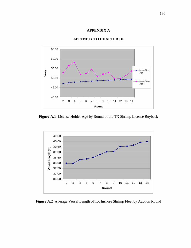
180
APPENDIX A
APPENDIX TO CHAPTER III
40.00
45.00
50.00
55.00
60.00
65.00
2 3 4 5 6 7 8 9 10 11 12 13 14
Round
Yea
rs Mean FleetAge
Mean SellerAge
Figure A.1 License Holder Age by Round of the TX Shrimp License Buyback
36.50
37.00
37.50
38.00
38.50
39.00
39.50
40.00
40.50
2 3 4 5 6 7 8 9 10 11 12 13 14
Round
Ves
sel L
ength
(ft
.)
Figure A.2 Average Vessel Length of TX Inshore Shrimp Fleet by Auction Round
181
VITA
Name: Aaron T. Mamula
Address: National Marine Fisheries Service Southwest Fisheries Science Center 110 Shaffer Road Santa Cruz, CA 95060 Email Address: [email protected] Education: B.A., Economics, Oregon State University, 2000 M.A., Economics, Southern Methodist University, 2003 Ph.D, Texas A&M University, 2009