li, y. and ang, k.h. and chong, g.c.y. (2006) pid control system analysis and design...

Li, Y. and Ang, K.H. and Chong, G.C.Y. (2006) PID control system analysis and design. IEEE Control Systems Magazine 26(1):pp. 32-41.

http://eprints.gla.ac.uk/3815/ Deposited on: 13 November 2007

Glasgow ePrints Service http://eprints.gla.ac.uk

32 IEEE CONTROL SYSTEMS MAGAZINE » FEBRUARY 2006 1066-033X/06/$20.00©2006IEEE

PID Control SystemAnalysis and Design

©IM

AG

ES

TA

TE

PID Control System Analysis and DesignPROBLEMS, REMEDIES, AND FUTURE DIRECTIONS

With its three-term functionality offering treatment of both transient and steady-state responses,

proportional-integral-derivative (PID) control provides a generic and efficient solution to real-world control problems [1]–[4]. The wide application of PID control has stimulated and sus-tained research and development to “get the best out of PID’’ [5], and “the search is on to findthe next key technology or methodology for PID tuning” [6].

This article presents remedies for problems involving the integral and derivative terms. PID design objec-tives, methods, and future directions are discussed. Subsequently, a computerized, simulation-based approachis presented, together with illustrative design results for first-order, higher order, and nonlinear plants. Finally,we discuss differences between academic research and industrial practice, so as to motivate new researchdirections in PID control.

STANDARD STRUCTURES OF PID CONTROLLERS

Parallel Structure and Three-Term FunctionalityThe transfer function of a PID controller is often expressed in the ideal form

By YUN LI, KIAM HEONG ANG, and GREGORY C.Y. CHONG

FEBRUARY 2006 « IEEE CONTROL SYSTEMS MAGAZINE 33

GPID(s) = U(s)E(s)

= KP

(1 + 1

TIs+ TD s

), (1)

where U(s) is the control signal acting on the error signal E(s),KP is the proportional gain, TI is the integral time constant, TD

is the derivative time constant, and s is the argument of theLaplace transform. The control signal can also be expressed inthree terms as

U(s) = KPE(s) + KI1s

E(s) + KD sE(s)

= UP(s) + UI(s) + UD(s), (2)

where KI = KP/TI is the integral gain and KD = KPTD is thederivative gain. The three-term functionalities include:

1) The proportional term provides an overall control actionproportional to the error signal through the allpass gainfactor.

2) The integral term reduces steady-state errors throughlow-frequency compensation.

3) The derivative term improves transient response throughhigh-frequency compensation.

A PID controller can be considered as an extreme form of aphase lead-lag compensator with one pole at the origin andthe other at infinity. Similarly, its cousins, the PI and the PDcontrollers, can also be regarded as extreme forms of phase-lag and phase-lead compensators, respectively. However, themessage that the derivative term improves transient responseand stability is often wrongly expounded. Practitioners havefound that the derivative term can degrade stability whenthere exists a transport delay [4], [7]. Frustration in tuning KD

has thus made many practitioners switch off the derivativeterm. This matter has now reached a point that requires clarifi-cation, as discussed in this article. For optimum performance,KP, KI (or TI), and KD (or TD) must be tuned jointly, althoughthe individual effects of these three parameters on the closed-loop performance of stable plants are summarized in Table 1.

The Series StructureIf TI ≥ 4TD, the PID controller can also be realized in a seriesform [7]

GPID(s) = (α + TD s) KP

(1 + 1

αTIs

)(3)

= GPD(s)GPI(s), (4)

where GPD(s) and GPI(s) are the factored PD and PI parts ofthe PID controller, respectively, and

α = 1 ± √1 − 4TD/TI

2> 0.

THE INTEGRAL TERM

Destabilizing Effect of the Integral TermReferring to (1) for TI �= 0 and TD = 0, it can be seen thatadding an integral term to a pure proportional term increasesthe gain by a factor of

∣∣∣∣1 + 1jωTI

∣∣∣∣ =√

1 + 1ω2T2

I

> 1, for all ω, (5)

and simultaneously increases the phase-lag since

�(

1 + 1jωTI

)= tan−1

( −1ωTI

)< 0, for all ω. (6)

Hence, both gain margin (GM) and phase margin (PM) arereduced, and the closed-loop system becomes more oscillatoryand potentially unstable.

Integrator Windup and RemediesIf the actuator that realizes the control action has saturatedrange limits, and the saturations are neglected in a linear con-trol design, the integrator may suffer from windup; this caus-es low-frequency oscillations and leads to instability. Thewindup is due to the controller states becoming inconsistentwith the saturated control signal, and future correction isignored until the actuator desaturates.

Automatic Reset If TI ≥ 4TD so that the series form (3) exists, antiwindup can beachieved implicitly through automatic reset. The factored PIpart of (3) is thus implemented as shown in Figure 1 [8], [9].

Explicit AntiwindupIn nearly all commercial PID software packages and hardwaremodules, however, antiwindup is implemented explicitlythrough internal negative feedback, reducing UI(s) to [8]–[10]

TABLE 1 Effects of independent P, I, and D tuning on closed-loop response.For example, while K I and K D are fixed, increasing K P alone can decrease rise time,increase overshoot, slightly increase settling time, decrease the steady-state error, and decrease stability margins.

Rise Time Overshoot Settling Time Steady-State Error StabilityIncreasing K P Decrease Increase Small Increase Decrease Degrade

Increasing K I Small Decrease Increase Increase Large Decrease Degrade

Increasing K D Small Decrease Decrease Decrease Minor Change Improve

34 IEEE CONTROL SYSTEMS MAGAZINE » FEBRUARY 2006

UI(s) = 1TIs

[KPE(s) − U(s) − U(s)

γ

], (7)

where U(s) is the theoretically computed control signal, U(s)is the actual control signal capped by the actuator limits, andγ is a correcting factor. A value of γ in the range [0.1, 1.0] usu-ally results in satisfactory performance when the PID coeffi-cients are reasonably tuned [7].

Accounting for Windup in Design SimulationsAnother solution to antiwindup is to reduce the possibilitiesfor saturation by reducing the control signal, as in linearquadratic optimal control schemes that minimize the trackingerror and control signal through a weighted objective func-tion. However, preemptive minimization of the control signalcan impede performance due to minimal control amplitude.Therefore, during the design evaluation and optimizationprocess, the control signal should not be minimized butrather capped at the actuator limits when the input to theplant saturates since a simulation-based optimization processcan automatically account for windup that might occur.

THE DERIVATIVE TERM

Stabilizing and Destabilizing Effect of the Derivative TermDerivative action is useful for providing phase lead, whichoffsets phase lag caused by integration. This action is alsohelpful in hastening loop recovery from disturbances. Deriva-tive action can have a more dramatic effect on second-orderplants than first-order plants [9].

However, the derivative term is often misunderstood andmisused. For example, it has been widely perceived in thecontrol community that the derivative term improves tran-sient performance and stability. But this perception is notalways valid. To see this, note that adding a derivative term toa pure proportional term reduces the phase lag by

�(1 + jωTD

) = tan−1 ωTD

1∈ [0, π/2] for all ω, (8)

which tends to increase the PM. In the meantime, however,the gain increases by a factor of

∣∣1 + jωTD∣∣ =

√1 + ω2T2

D > 1, for all ω, (9)

and hence the overall stability may be improved or degraded.To demonstrate that adding a differentiator can destabilize

some systems, consider the typical first-order delayed plant

G(s) = K1 + Ts

e−Ls, (10)

where K is the process gain, T is the time constant, and L is thedead time or transport delay. Suppose that this plant is con-trolled by a proportional controller with gain KP and that aderivative term is added. The resulting PD controller

GPD(s) = KP(1+TD s) (11)

leads to an open-loop feedforward path transfer function withfrequency response

G( jω)GPD( jω) = KKP1 + jTDω

1 + jTωe− jLω. (12)

For all ω, the gain satisfies

KKP

√1 + T2

Dω2

1 + T2ω2� KKP min

(1,

TD

T

), (13)

where inequality (13) holds since ((1 + T2Dω2)/(1 + T2ω2))

1/2 ismonotonic in ω.

Hence, if KP > 1/K and TD > T/K KP, then, for all ω,

∣∣G( jω)GPD( jω)∣∣ > 1. (14)

Inequality (14) implies that the 0-dB gain crossover frequency isat infinity. Furthermore, due to the transport delay, the phase is

� G( jω)GPD( jω) = tan−1 ωTD1 − tan−1 Tω

1 − Lω.

Therefore, when ω approaches infinity,

� G( jω)GPD( jω) < −180◦. (15)

Hence, if TD > T/KKP and KP > 1/K, then by the Nyquist crite-rion, the closed-loop system is unstable. This analysis also con-firms that some PID mapping formulas, such as theZiegler-Nichol (Z-N) formula obtained from the step-responsemethod, in which KP = (1.2(T/L))(1/K) and TD is proportionalto L, are valid for only a limited range of values of the T/L ratio.

As an example, consider plant (10) with K = 10, T = 1 s, andL = 0.1 s [7]. Control by means of a PI controller with KP =0.644 > 1/K and TI = 1.03 s yields reasonable stability marginsand time-domain performance, as seen in Figures 2 and 3 (Set 1,red curves). However, when a differentiator is added, gradually

FIGURE 1 The PI part of a PID controller in series form for automaticreset. The PI part of a PD-PI factored PID transfer function can beconfigured to counter actuator saturation without the need for sepa-rate antiwindup action. Here, UPD(s) is the control signal from thepreceding PD section. When U(s) does not saturate, the feedfor-ward-path gain is unity and the overall transfer function from UPD(s)

to U(s) is thus 1 + 1/(αTIs), the same as the last factor of (3).

++

U(s)U(s)Actuator Model

UPD(s)

1

1 + α TIs

KP


increasing TD from zero improves both GM and PM. The GMpeaks when TD approaches 0.03 s; this value of TD maximizesthe speed of the transient response without oscillation. Howev-er, if TD is increased further to 0.1 s, the GM deteriorates andthe transient exhibits oscillation. In fact, the closed-loop systemcan be destabilized if TD increases to 0.2 with T/KKP = 0.155.Hence, care needs to be taken to tune and use the derivativeterm properly when the plant is subject to delay.

This destabilizing phenomenon can contribute to difficul-ties in designing PID controllers. These difficulties help explainwhy 80% of PID controllers in use have the derivative partswitched off or omitted completely [5]. Thus, the functionalityand potential of a PID controller is not fully exploited, whileproper use of a derivative term can increase stability and helpmaximize the integral gain for better performance [11].

Remedies for Derivative ActionDifferentiation increases the high-frequency gain, as shown in(9) and demonstrated by the four sets of frequency responsesin Figure 2. A pure differentiator is not proper or causal.When a step change of the setpoint or disturbance occurs, dif-ferentiation results in a theoretically infinite control signal. Toprevent this impulse control signal, most PID software pack-ages and hardware modules add a filter to the differentiator.Filtering is particularly useful in a noisy environment.

Linear Lowpass FilterThe filtering remedy most commonly adopted is to cascadethe differentiator with a first-order, lowpass filter, a techniqueoften used in preprocessing for data acquisition. Hence, thederivative term becomes

GD(s) = KPTD s

1 + TDβ

s, (16)

where β is a constant factor. Most industrial PID hardwareprovides a value ranging from 1 to 33, with the majorityfalling between 8 and 16 [12]. A second-order Butterworthfilter is recommended in [13] if further attenuation of high-frequency gains is required. Sometimes, the lowpass filter iscascaded to the entire GPID in internal-model-control (IMC)-based design, which therefore leads to more sluggish tran-sients.

Velocity FeedbackBecause a lowpass filter does not completely remove, butrather averages, impulse derivative signals caused by sud-den changes of the setpoint or disturbance, modifications ofthe unity negative feedback PID structure are of interest [8].To block the effect of sudden changes of the setpoint, weconsider a variant of the standard feedback. This variant uses

FIGURE 2 Destabilizing effect of the derivative term, measured in the frequency domain by GM and PM. Adding a derivative term increasesboth the GM and PM, although raising the derivative gain further tends to reverse the GM and destabilize the closed-loop system. Forexample, if the derivative gain is increased to 20% of the proportional gain (TD = 0.2 s), the overall open-loop gain becomes greater than2.2 dB for all ω. At ω = 30 rad/s, the phase decreases to −π while the gain remains above 2.2 dB. Hence, by the Nyquist criterion, theclosed-loop system is unstable. It is interesting to note that MATLAB does not compute the frequency response as shown here, since MAT-LAB handles the transport delay factor e−jωL in state space through a Padé approximation.

Set 1: TD = 0

PIDeasy: TD = 0.0303

Set 2: TD = 0.1

Set 3: TD = 0.2

Nichols Chart

PIDeasy(TM) II - Nichols Chart

Nichols Chart

Set 1Set 1:

Set 2:

Set 3:

PIDeasy

PIDeasy:Set 2Set 3

Gain Margin: 7.75757Phase Margin: 53.37157

Gain Margin: −2.26496Phase Margin: – ∞



40

30

20

Gai

n (d

B)

10

0

−10

−20−3.5 −2.5 −2.0

Phase (deg.)

−1.5 −1.0 −0.5

×102

0.0−3.0


the process variable instead of the error signal for the deriva-tive action [14], as in

u(t) = KP e(t) + KI

∫ t

0e(τ) dτ − KD

ddt

y(t), (17)

where y(t) is the process variable, e(t) = r(t) − y(t) is the errorsignal, and r(t) is the setpoint or reference signal. The last termof (17) forms velocity feedback and, hence, an extra loop thatis not directly affected by a sudden change in the setpoint.However, sudden changes in disturbance or noise at the plantoutput can cause the differentiator to produce a theoreticallyinfinite control signal.

Setpoint FilterTo further reduce sensitivity to setpoint changes and avoidovershoot, a setpoint filter may be adopted. To calculate theproportional action, the setpoint signal is weighted by a factorb < 1, as in [8] and [14]

u(t) = KP(b r(t) − y(t)

) + KI∫ t

0 e(τ) dτ − KDddt

y(t). (18)

This modification results in a bumpless control signal andimproved transients if the value of b is carefully chosen [2].However, modification (18) is difficult to analyze quantita-

tively using standard techniques of stability and robust-ness analysis.

Structure (17) is referred to as Type B PID (or PI-D) control,structure (18) is known as Type C PID (or I-PD) control, andstructures (1)–(3) constitute Type A PID control. Types B and Cintroduce more structures, and the need for preselection of, orswitching between, suitable structures can pose a design chal-lenge. To meet this need, PID hardware vendors have developedartificial intelligence techniques to suppress overshoots [15], [16].

Nevertheless, the ideal, parallel, series, and modified PID con-troller structures can be found in many software packages andhardware modules. Techmation’s Applications Manual [12] docu-ments the structures employed in many industrial PID con-trollers. Since vendors often recommend their own controllerstructures, tuning rules for a specific structure do not necessarilyperform well with other structures. Readers may refer to [17] and[18] for detailed discussions on the use of various PID structures.

PrefilterFor setpoint tracking applications, an alternative to using a TypeB or C structure is to cascade the setpoint with a prefilter thathas critically damped dynamics. When a step change in the set-point occurs, continuous output of the prefilter helps achievesoft start and bumpless control [8], [19]. However, a prefilterdoes not solve the problem caused by sudden changes in thedisturbance since it is not embedded in the feedback loop.

FIGURE 3 Destabilizing effect of the derivative term, confirmed in the time domain by the closed-loop step response. Although increasing thederivative gain initially decreases the oscillation, this trend soon reverses and the oscillation grows into instability.

Set 1: TD = 0

Set 2: TD = 0.1

Set 3: TD = 0.2PIDeasy: TD = 0.0303

Sampling Rate: 0.00014 sec.View Both Responses

PIDeasy(TM) II - Step and Control Signal Response Dialog

Step Response

Step Response Plot

Set 1:

Set 2:

Set 3:

Set 1

Set 2

Set 3

PIDeasy:PIDeasy

Kp: 0.6439Ti: 1.0278Td: 0.2ITAE: 52,547.83

Kp: 0.6439Ti: 1.0278Td: 0.1ITAE: 247.69

Kp: 0.6439Ti: 1.02781Td: 0.03025ITAE: 104.86

Kp: 0.6439Ti: 1.0278Td: 0ITAE: 228.93

1.4

1.2

1.0

0.8

0.6

0.4

Out

put

0.2

0.0

0.0 0.2 0.4 0.6

Time (Sec.)

0.8 1.0 1.2 1.4


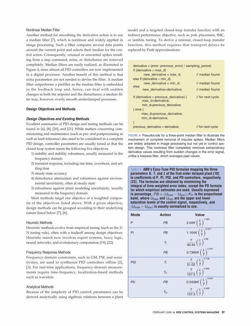
Nonlinear Median FilterAnother method for smoothing the derivative action is to usea median filter [7], which is nonlinear and widely applied inimage processing. Such a filter compares several data pointsaround the current point and selects their median for the con-trol action. Consequently, unusual or unwanted spikes result-ing from a step command, noise, or disturbance are removedcompletely. Median filters are easily realized, as illustrated inFigure 4, since almost all PID controllers are now implementedin a digital processor. Another benefit of this method is thatextra parameters are not needed to devise the filter. A medianfilter outperforms a prefilter as the median filter is embeddedin the feedback loop and, hence, can deal with suddenchanges in both the setpoint and the disturbance; a median fil-ter may, however, overly smooth underdamped processes.

Design Objectives and Methods

Design Objectives and Existing MethodsExcellent summaries of PID design and tuning methods can befound in [4], [8], [20], and [21]. While matters concerning com-missioning and maintenance (such as pre- and postprocessing aswell as fault tolerance) also need to be considered in a completePID design, controller parameters are usually tuned so that theclosed-loop system meets the following five objectives:

1) stability and stability robustness, usually measured in thefrequency domain

2) transient response, including rise time, overshoot, and set-tling time

3) steady-state accuracy4) disturbance attenuation and robustness against environ-

mental uncertainty, often at steady state5) robustness against plant modeling uncertainty, usually

measured in the frequency domain.Most methods target one objective or a weighted compos-

ite of the objectives listed above. With a given objective,design methods can be grouped according to their underlyingnature listed below [7], [8].

Heuristic MethodsHeuristic methods evolve from empirical tuning (such as the Z-N tuning rule), often with a tradeoff among design objectives.Heuristic search now involves expert systems, fuzzy logic,neural networks, and evolutionary computation [19], [22].

Frequency Response MethodsFrequency-domain constraints, such as GM, PM, and sensi-tivities, are used to synthesize PID controllers offline [2],[3]. For real-time applications, frequency-domain measure-ments require time-frequency, localization-based methodssuch as wavelets.

Analytical MethodsBecause of the simplicity of PID control, parameters can bederived analytically using algebraic relations between a plant

model and a targeted closed-loop transfer function with anindirect performance objective, such as pole placement, IMC,or lambda tuning. To derive a rational, closed-loop transferfunction, this method requires that transport delays bereplaced by Padé approximations.

FIGURE 4 Pseudocode for a three-point median filter to illustrate themechanism of complete removal of impulse spikes. Median filtersare widely adopted in image processing but not yet in control sys-tem design. This nonlinear filter completely removes extraordinaryderivative values resulting from sudden changes in the error signal,unlike a lowpass filter, which averages past values.

derivative = (error -previous_error) / sampling_period;if (derivative > max_d)

new_derivative = max_d; // median foundelse if (derivative < min_d)

new_derivative = min_d; // median found

// median foundelse

new_derivative=derivative;

if (derivative > previous_derivative) { // for next cyclemax_d=derivative;min_d=previous_derivative;

} else {max_d=previous_derivative;min_d=derivative;

}previous_derivative = derivative; // for next cycle

TABLE 2 ABB’s Easy-Tune PID formulas mapping the threeparameters K, T, and L of the first-order delayed plant (10)to coefficients of P, PI, PID, and PD controllers, respectively[23]. The formulas are obtained by minimizing the integral of time-weighted error index, except the PD formulafor which empirical estimates are used. Usually expressedin percentage, PB = (Umax − Umin)/K P is the proportionalband, where Umax and Umin are the upper and lowersaturation levels of the control signal, respectively, and|Umax − Umin| is usually normalized to one.

Mode Action Value

P PB 2.04K(

LT

)1.084

PI PB 1.164K(

LT

)0.977

TIT

40.44

(LT

)0.68

PB 0.7369K(

LT

)0.947

PID TIT

51.02

(LT

)0.738

TDT

157.5

(LT

)0.995

PD PB 0.5438K(

LT

)0.947

TDT

157.5

(LT

)0.995

Numerical Optimization MethodsOptimization-based methods can be regarded as a special typeof optimal control. PID parameters are obtained by numericaloptimization for a weighted objective in the time domain.Alternatively, a self-learning evolutionary algorithm (EA) canbe used to search for both the parameters and their associatedstructure or to meet multiple design objectives in both the

time and frequency domains [19], [22].Some design methods can be computerized, so that designs

are automatically performed online once the plant is identified;hence, these designs are suitable for adaptive tuning. WhilePID design has progressed from analysis-based methods tonumerical optimization-based methods, there are few tech-niques that are as widely applicable as Z-N tuning [2], [3]. The

most widely adopted initial tuning methods are basedon the Z-N empirical formulas and their extensions, suchas those shown in Table 2 [23]. These formulas offer adirect mapping from plant parameters to controller coef-ficients.

Over the past half century, researchers have sought thenext key technology for PID tuning and modular realiza-tion [6]. With simulation packages widely available andheavily adopted, computerizing simulation-based designsis gaining momentum, enabling simulations to be carriedout automatically so as to search for the best possible PIDsettings for the application at hand [22]. By using a com-puterized approach, multiple design methods can be com-bined within a single software or firmware package tosupport various plant types and PID structures.

A Computerized Simulation ApproachPIDeasy [7] is a software package that uses automatic sim-ulations to search globally for controllers that meet all fivedesign objectives in both the time and frequency domains.The search is initially performed offline in a batch mode[19] using artificial evolution techniques that evolve both

FIGURE 5 Gain and phase margins resulting from PIDeasy designs for first-order delayed plants with various L/T ratios. While requirements of fasttransient response, no overshoot, and zero steady-state error are accom-modated by time-domain criteria, multiobjective design goals providefrequency-domain margins in the range of 9–11 dB and 65–66◦.

80

5

10

15

70

60

50

L/T

10−3 10−2 10−1 100 101 102 103

10−3 10−2 10−1 100 101 102 103

Pha

se M

argi

n (°

)G

ain

Mar

gin

(dB

)

TABLE 3 Multioptimal PID settings for normalized typical high-order plants. Since PIDeasy’s search priorities are time-domaintracking and regulation, the corresponding gain and phase margins are given to assess frequency-domain properties.

PID Coefficients Resultant MarginsPlants Kp Ti (s) Td (s) GM (dB) PM (◦)

G1(s) = 1(s + 1)α

α = 1 92.1 1.0 0.0022 ∞ 102α = 2 1.95 1.61 0.14 ∞ 62.4α = 3 1.12 2.13 0.28 26.8 60.7α = 4 0.83 2.61 0.43 13.9 61α = 8 0.50 4.31 1.01 9.05 58.9

G2(s) = 1(s + 1)(1 + αs)(1 + α2s)(1 + α3s)

α = 0.1 5.53 1.03 0.04 52.8 68.7α = 0.2 2.87 1.08 0.07 38.6 66.3α = 0.5 1.19 1.36 0.17 19.1 62.6

G3(s) = 1 − αs(s + 1)3

α = 0.1 1.03 2.15 0.31 19.4 61.2α = 0.2 0.96 2.18 0.33 16.6 61.6α = 0.5 0.79 2.23 0.39 13 62.4α = 1.0 0.63 2.30 0.47 7.52 50.9α = 2.0 0.48 2.39 0.57 7.45 58.6α = 5.0 0.36 2.58 0.72 2.69 40.4

G4(s) = 1(1 + sα)2

e−s

α = 0.1 0.23 0.43 0.12 10.4 66α = 0.2 0.30 0.59 0.17 10.4 65.8α = 0.5 0.49 1.07 0.26 10.5 65.6α = 2.0 1.04 3.49 0.49 15 62.4α = 5.0 1.42 8.32 0.92 24.2 62.1α = 10 1.65 16.35 1.59 32.8 62.1



controller parameters and their associated structures. For practi-cal simplicity and reliability, the standard PID structure is main-tained as much as possible, while allowing augmentation witheither lowpass or median filtering for the differentiator and withexplicit antiwindup for the integrator. The resulting designs arethen embedded in the PIDeasy package. Further specific tuningcan be continued by local, fast numerical optimization if theplant differs from its model or data used in the initial design.

First-Order Delayed PlantsAn example of PIDeasy for a first-order delayed plant isshown in Figures 2 and 3. To assess the robustness of designusing PIDeasy, GMs and PMs resulting from designs forplants with various L/T ratios are shown in Figure 5 [19].While requirements of fast transient response, no overshoot,and zero steady-state error are accommodated by time-domain criteria, PIDeasy’s multiobjective goals provide fre-quency-domain margins in the range of 9–11 dB and 65–66◦.

Higher Order PlantsFor higher order plants, we obtain multioptimal designs forthe 20 benchmark plants [24]

G1(s) = 1(s + 1)α

, α = 1, 2, 3, 4, 8, (19)

G2(s) = 1(s + 1)(1 + αs)(1 + α2s)(1 + α3s)

,

α = 0.1, 0.2, 0.5, (20)

G3(s) = 1 − αs(s + 1)3

, α = 0.1, 0.2, 0.5, 1, 2, 5, (21)

G4(s) = 1(1 + sα)2

e−s, α = 0.1, 0.2, 0.5, 2, 5, 10. (22)

The resulting designs and their corresponding gain and PMsare summarized in Table 3.

Setpoint-Scheduled PID Network Consider the constant-temperature reaction process

dy(t)dt

= −Ky2(t) + 1V

[d − y(t)

]u(t), (23)

wherey(t) = concentration in the outlet stream (mol/�),u(t) = flow rate of the feed stream (�/h),K = rate of reaction (�/mol-h),V = reactor volume (� ),d = concentration in the inlet stream (mol/� ).

The setpoint, equilibrium, or steady-state operating trajectoryof the plant is governed by

Ky2 + 1V

u y − dV

u = 0. (24)

For setpoints ranging from 0 to 1 mol/�, an initial PIDcontroller can be placed effectively at y = 0.49 by using themaximum distance from the nonlinear trajectory to the lin-

ear projection linking the starting and ending points of theoperating envelope, as illustrated by node 2 in Figure 6 [22].Similarly, two more controllers can be added at nodes orsetpoints 1 and 3, forming a pseudolinear controller net-work comprised of three PIDs to be interweighted by sched-uling functions S1(y), S2(y), and S3(y), examples of which areshown in Figure 7.

FIGURE 6 Operating trajectory (bold curve) of the nonlinear chemicalprocess (23) for setpoints ranging from 0 to 1 mol/�, as given by(24). A PID controller is first placed at y = 0.49 (node 2) by usingthe maximum distance from the nonlinear trajectory to the linearprojection (thin dotted line) linking the starting and ending points ofthe operating envelope. Similarly, two more controllers can beadded at nodes 1 and 3, forming a pseudo-linear controller networkcomprised of three PIDs. Without the need for linearization, thesePID controllers can be obtained individually by PIDeasy or other PIDsoftware directly through step-response data, or obtained jointly byusing an evolutionary algorithm [22].

0 1 2 3 4 5 60

0.1

0.2

0.3

0.4

0.5

0.6

0.7

0.8

0.9

1

Input (l/h)

0.74

0.49

0.31

∆dmax

3

2

1

Out

put (

mol

/l )

FIGURE 7 Fuzzy logic membership-like scheduling functions S1(y),S2(y), and S3(y) for individual PID controllers contributing to thePID network at nodes 1, 2, and 3, respectively. Due to nonlinearity,these functions are often asymmetric. Similar to gain scheduling, lin-ear interpolation suffices for setpoint scheduling.

0.90.80.70.60.50.40.30.20.10

0

0.2

0.4

0.6

0.8

1

0.31 0.49 0.74

Scheduling Variable y (mol/l)

S1 S2 S3

Wei

ghtin

g


The PID controller centered at node 2 can be obtained byPIDeasy or other PID software directly through step-responsedata without the need for linearization at the current operating

point [22]. The remaining PIDs can be obtained similarly. Forsimplicity, we obtain the controller centered at node x, wherex = 1, 2, and 3, by using step-response data from the startingpoint to node x. The resulting PID network is given by

u(t) = [S1 S2 S3]

[ 9.82 1.22 0.037615.6 0.784 0.024128.6 0.481 0.0137

] [ 1p−1

p

]e(t),

(25)

where p denotes the derivative operator. To validate tracking performance using a setpoint that is

not originally used in the design process, the setpoint r = 0.53mol/� is used to test the control system. The response isshown in Figure 8, where a 10% disturbance occurs during [3,3.5] h, confirming load disturbance rejection at steady state.Figure 9 shows the performance of the network at multipleoperating levels not originally encountered in the design. If amore sophisticated PID network is desirable, the number ofnodes, controller parameters for each node, and schedulingfunctions can be optimized globally in a single design processby using an EA [22].

It is known that gain scheduling provides advantages overcontinuous adaptation in most situations [8]. The setpoint-scheduled network utilizes these advantages of gain schedul-ing. Furthermore, by bumpless scheduling, the network doesnot require discontinuous switching between various con-troller structures.

Discussion and ConclusionsPID is a generally applicable control technique thatderives its success from simple and easy-to-under-stand operation. However, because of limited infor-mation exchange and problem analysis, thereremain misunderstandings between academia andindustry concerning PID control. For example, themessage that increasing the derivative gain leads toimproved transient response and stability is oftenwrongly expounded. These misconceptions mayexplain why the argument exists that academicallyproposed PID tuning rules sometimes do not workwell on industrial controllers. In practice, therefore,switching between different structures and func-tional modes is used to optimize transient responseand meet multiple objectives.

Difficulties in setting optimal derivative actioncan be eased by complete understanding and carefultuning of the D term. Median filtering, which iswidely adopted for preprocessing in image process-ing but yet to be adopted in controller design, is aconvenient tool for solving problems that the PI-Dand I-PD structures are intended to address. A medi-an filter outperforms a lowpass filter in removingimpulse spikes of derivative action resulting from asudden change of setpoint or disturbance. Embedded

FIGURE 8 Performance of the pseudolinear PID network applied tothe nonlinear process example (23). To validate tracking perfor-mance using a setpoint that is not originally used in the designprocess, the setpoint r = 0.53 mol/� is used to test the control sys-tem. The controller network tracks this setpoint change accuratelywithout oscillation and rejects a 10% load disturbance occurringduring [3, 3.5] h.

0 0.5 1 1.5 2 2.5 3 3.5 4 4.5 50

0.2

0.4

0.6 0.53

0.8

Time (h)

0 0.5 1 1.5 2 2.5 3 3.5 4 4.5 5Time (h)

Out

put (

mol

l−1)

0

2

4

6

Con

trol

Sig

nal (

l h−1

)

FIGURE 9 Performance of the pseudolinear PID network applied to the nonlin-ear chemical process (23) at multiple operating levels that are not originallyused in the design process. The network tracks these setpoint changes accu-rately without oscillation. It can be seen that the control effort increases dispro-portionally to the setpoint change along the nonlinear trajectory, compensatingfor the decreasing gain of the plant when the operating level is raised.

0

0.5

0.9

0.6

0.3

1

Out

put m

ol (

l−1)

0 1 2 3 4 5 6 7 8 90

2

4

6

8

10

Time (h)

0 1 2 3 4 5 6 7 8 9Time (h)

Con

trol

Sig

nal (

l h−1

)


in the feedback loop, a median filter also outperforms a pre-filter in dealing with disturbances.

Over the past half century, researchers have sought thenext key technology for PID tuning and modular realization.Many design methods can be computerized and, with simula-tion packages widely used, the trend of computerizing simu-lation-based designs is gaining momentum. Computerizingenables simulations to be carried out automatically, whichfacilitates the search for the best possible PID settings for theapplication at hand. A simulation-based approach requires noartificial minimization of the control amplitude and helpsimprove sluggish transient response without windup.

In tackling PID problems, it is desirable to use standardPID structures for a reasonable range of plant types and oper-ations. Modularization around standard PID structuresshould also help improve the cost effectiveness of PID controland maintenance. This way, robustly optimal design methodssuch as PIDeasy can be developed. By including system iden-tification techniques, the entire PID design and tuning processcan be automated, and modular code blocks can be madeavailable for timely application and real-time adaptation.

ACKNOWLEDGMENTSThis article is based on [25]. Kiam Heong Ang and GregoryChong are grateful to the University of Glasgow for a post-graduate research scholarship and to Universities UK for anOverseas Research Students Award. The authors thank Prof.Hiroshi Kashiwagi of Kumamoto University and MitsubishiChemical Corp., Japan, for the nonlinear reaction processmodel and data.

AUTHOR INFORMATIONYun Li ([email protected]) is a senior lecturer at the Universi-ty of Glasgow, United Kingdom, where he has taught andconducted research in evolutionary computation and controlengineering since 1991. He worked in the U.K. National Engi-neering Laboratory and Industrial Systems and Control Ltd,Glasgow, in 1989 and 1990. In 1998, he established the IEEECACSD Evolutionary Computation Working Group and theEuropean Network of Excellence in Evolutionary Computing(EvoNet) Workgroup on Systems, Control, and Drives. Hewas a visiting professor at Kumamoto University, Japan. He iscurrently a visiting professor at the University of ElectronicScience and Technology of China. His research interests are inparallel processing, design automation, and discovery of engi-neering systems using evolutionary learning and intelligentsearch techniques. He has advised 12 Ph.D. students and has140 publications. He can be contacted at the Department ofElectronics and Electrical Engineering, University of Glasgow,Glasgow G12 8LT, U.K.

Kiam Heong Ang received a First-Class Honors B.Eng. anda Ph.D. degree in electronics and electrical engineering fromthe University of Glasgow, United Kingdom, in 1996 and2005, respectively. From 1997–2000, he was a software engi-neer with Advanced Process Control Group, Yokogawa Engi-

neering Asia Pte. Ltd., Singapore. Since 2005, within the samecompany, he has been working on process industry stand-ardization and new technology development. His researchinterests include evolutionary, multiobjective learning, com-putational intelligence, control systems, and engineeringdesign optimization.

Gregory Chong received a First-Class Honors B.Eng. degreein electronics and electrical engineering from the University ofGlasgow, United Kingdom, in 1999. He is completing hisPh.D. at the same university in evolutionary, multiobjectivemodeling, and control for nonlinear systems.

REFERENCES[1] J.G. Ziegler and N.B. Nichols, “Optimum settings for automatic con-trollers,” Trans. ASME, vol. 64, no. 8, pp. 759–768, 1942.[2] W.S. Levine, Ed., The Control Handbook. Piscataway, NJ: CRC Press/IEEEPress, 1996.[3] L. Wang, T.J.D. Barnes, and W.R. Cluett, “New frequency-domain designmethod for PID controllers,” Proc. Inst. Elec. Eng., pt. D, vol. 142, no. 4, pp.265–271, 1995.[4] J. Quevedo and T. Escobet, Eds., “Digital control: Past, present and futureof PID control,” in Proc. IFAC Workshop, Terrassa, Spain, Apr. 5, 2000. [5] I.E.E. Digest, “Getting the best out of PID in machine control,” in DigestIEE PG16 Colloquium (96/287), London, UK, Oct. 24, 1996. [6] P. Marsh, “Turn on, tune in—Where can the PID controller go next,” NewElectron., vol. 31, no. 4, pp. 31–32, 1998.[7] Y. Li, W. Feng, K.C. Tan, X.K. Zhu, X. Guan, and K.H. Ang, “PIDeasy andautomated generation of optimal PID controllers,” in Proc. 3rd Asia-PacificConf. Control and Measurement, Dunhuang, P.R. China, 1998, pp. 29–33.[8] K.J. Åström and T. Hägglund, PID Controllers: Theory, Design, and Tuning.Research Triangle Park, NC: Instrum. Soc. Amer., 1995.[9] F.G. Shinskey, Feedback Controllers for the Process Industries. New York:McGraw-Hill, 1994.[10] C. Bohn and D.P. Atherton, “An analysis package comparing PID anti-windup strategies,” IEEE Contr. Syst. Mag., vol. 15, no. 2, pp. 34–40, Apr.1995.[11] K.J. Åström and T. Hägglund, “The future of PID control,” Contr. Eng.Pract., vol. 9, no. 11, pp. 1163–1175, 2001.[12] Techmation Inc., Techmation [Online], May 2004. Available: http://pro-tuner.com[13] J.P. Gerry and F.G. Shinskey, “PID controller specification,” white paper[Online]. May 2004. Available: http://www.expertune.com/PIDspec.htm[14] BESTune, PID controller tuning [Online]. May 2004. Available:http://bestune.50megs.com[15] Honeywell International Inc. [Online]. May 2004. Available: http://www.Acs.Honeywell.Com/Ichome/Rooms/DisplayPages/LayoutInitial[16] Y. Li, K.H. Ang, and G. Chong, “Patents, software, and hardware forPID control,” IEEE Contr. Syst. Mag., vol. 26, no. 1, pp. 42–54, 2006. [17] J.P. Gerry, “A comparison of PID control algorithms,” Contr. Eng., vol.34, no. 3, pp. 102–105, Mar. 1987.[18] A. Kaya and T.J. Scheib, “Tuning of PID controls of different structures,”Contr. Eng., vol. 35, no. 7, pp. 62–65, July 1988.[19] W. Feng and Y. Li, “Performance indices in evolutionary CACSDautomation with application to batch PID generation,” in Proc. 10th IEEE Int.Symp. Computer Aided Control System, Hawaii, Aug. 1999, pp. 486–491.[20] R. Gorez, “A survey of PID auto-tuning methods,” Journal A, vol. 38, no. 1,pp. 3–10, 1997.[21] A. O’Dwyer, Handbook of PI and PID Controller Tuning Rules. London:Imperial College Press, 2003.[22] Y. Li, K.H. Ang, G. Chong, W. Feng, K.C. Tan, and H. Kashiwagi, “CAutoCSD—Evolutionary search and optimisation enabled computer-automated control system design,” Int. J. Automat. Comput., vol. 1, no. 1, pp. 76–88, 2004.[23] Specification Data File of Commander 355, ABB, SS/C355, Issue 3, 2001. [24] K.J. Åström and T. Hägglund, “Benchmark systems for PID control,” inProc. IFAC Workshop, Terrassa, Spain, 2000, pp. 165–166.[25] K.H. Ang, G. Chong, and Y. Li, “PID control system analysis, design, andtechnology,” IEEE Trans. Contr. Syst. Tech., vol. 13, no. 4, pp. 559–576, 2005.

li, y. and ang, k.h. and chong, g.c.y. (2006) pid control system analysis and design...

Documents