lógica no avião
TRANSCRIPT
An Introduction to PartiallyOrdered Structures andSheaves
Francisco Miraglia
Lógica no Avião

An Introduction to PartiallyOrdered Structures and Sheaves
Francisco Miraglia
Department of MathematicsUniversity of Sao Paulo
To
Tiago Passos Miraglia
In Memoriam
Editorial Board
Fernando FerreiraDepartamento de Matematica
Universidade de Lisboa
Francisco MiragliaDepartamento de Matematica
Universidade de Sao Paulo
Graham PriestDepartment of Philosophy
The City University of New York
Johan van BenthemDepartment of Philosophy Stanford University
Tsinghua UniversityUniversity of Amsterdam
Matteo VialeDipartimento di Matematica “Giuseppe Peano”
Universita di Torino
Francisco Miraglia, An Introduction to Partially Ordered
Structures and Sheaves, Brasılia: Logica no Avi~ao, 2020.
Serie L, Volume 2
I.S.B.N. 978-65-00-06148-2
Obra publicada com o apoio do PPGFIL/UnB.

Editorial Preface
I am very glad for the opportunity to write an editorial preface to “An In-troduction to Partially Ordered Structures and Sheaves” by Francisco Miraglia.This book with 45 chapters and almost 500 pages of exciting mathematics, featur-ing partially ordered structures, category theory, spectral spaces, presheaves overtopological spaces, change of base and characteristic maps, originated in graduatecourses given by the author, as a visiting scholar at the Mathematical Instituteof Oxford University, in the academic year 90/91. It was first published by Poli-metrica International Scientific Publisher in January 2009, where I was acting asa chief editor. I then had the privilege of writing a more careful, perhaps a bitpoetic, Foreword to the book. I will not repeat it here, but instead register somefacts. Polimetrica was founded by Giandomenico de Sica in Monza, Italy, withthe intention of bringing quality books to light. In my short life as an editor atPolimerica, I had the chance to publish, besides Miraglia’s book, also “The MagicGarden of George B And Other Logic Puzzles” by Raymond Smullyan in 2007,which was reprinted by World Scientific in 2015. Polimetrica did publish severalbooks, but unfortunately could not resist the pressure of the editorial market.
I would like to applaud the excellent initiative by the UnB Brasilia groupof “Logica no Aviao” (LnA) in the person of Rodrigo Freire (editor), AlexandreCosta-Leite, Edgar Almeida and Gustavo Schmidt in republishing this book. LnAis a non-profit organization dedicated to the promotion and dissemination of highquality work in logic and philosophy, and will make this extraordinary book freefor all future generations. I am proud to have contributed to it.
Campinas, July 2020
Walter Carnielli
5

Foreword
The discussion whether category theory is just a convenient language or hasits own intrinsic way to conceptualize mathematical knowledge will be seen as idleafter you read this book: you will certainly agree that it is both. Category theorywas born under the point of view that many (or all) concepts in Mathematics couldbe better understood and explained by approaching them in a highly unified way:several definitions, constructions, proofs and concepts are essentially the same, andthis is what the tools of category theory reveal.
Interesting enough, the idea of “category” derives from the use it had in phi-losophy; even if the intention the founders of category theory gave the term is notexactly the one Aristotle, Immanuel Kant, and Charles S. Peirce referred to it,some connections remain.
Perhaps what the ideas of category in the philosophical and mathematicalsenses share is the concern about existence and predication. In a similar way as onwhat can be said about a given object or subject, as idealized by the classics, woulddepend on the attention to certain aspects (such as quantity, substance, relationsor states), in the mathematical categories the existence of objects depends on theconceptual environment. The witnesses of their existence are the morphisms (an-other borrowed term, this one from R. Carnap) that relate the object in questionwith other objects.
Some authors will say that, in category theory, an object cannot say to exist,but what exists is the concept behind it. This is clearly reflected, for instance, insetting the natural number objects in sheaves: if we suspect that perhaps one ofthe most fundamental properties of natural numbers is their capacity of definingfunctions by recursion, an abstract treatment can test this idea and see how far itgoes.
It is in the spirit of Mathematics to stretch out the essence of an idea to itsultimate consequences: this way, for example, the category of sets or a topos ofsheaves over a topological space generalize at the same time a huge number ofconcepts.
This book gives an overall, as self-contained as possible, introduction to sheaftheory and its relation to logic. Starting from partially ordered structures, Mi-raglia shows how to go from lattices to sheaf theory, how this naturally leads tothe universal constructions of category theory, and to first-order structures overpartially ordered sets.
6
Foreword 7
Sheaves and presheaves over topological spaces - and how this is related tofirst-order structures - is a central topic of this book.
But the connections to contemporary logic itself go much further: A theory ofrelations and quantification in some particular categories is also explained; classi-cal existential and universal quantifiers arise from those when certain projections“forget” coordinates, following the seminal ideas of Francis William Lawvere onconceptual mathematics.
There is also a deep methodological point when working in abstract partiallyordered structures and sheaves, and this book contributes to making this pointclear - as in general such structures are “pointless”, the constructions and gener-alizations from elementary to more sophisticated results have to be more intrinsic,but this, on the other hand, reveals the common relationship among semillatices,distributive lattices, Heyting algebras and frames.
Continuous lattices and their natural topology (the “Scott topology”) is a ba-sic topic here; they are known to be connected with computer science, generaltopology, analysis, algebra and topos theory. This will also be relevant to read-ers interested in constructive mathematics, and in deeper connections betweencategory theory and Logic, and on how this leads to more abstract views, as forexample how the methods of homology, cohomology, algebra and topological K-theory could be seen as a sort of unified theory.
But what is an enjoyable and distinctive characteristic of this book is thatall this (and its relationship to category theory) is developed in a smooth way:Miraglia chooses to introduce sheaves directly as mathematical structures, (specif-ically, as Ω-sets closed under certain gluing properties) without previous require-ments on category theory, for the benefit of the non-acquainted reader. This makesthis book as peerless introduction not only to concepts and methods, but to thephilosophical assumptions, foundations and significance of contemporary logic.
Walter Carnielli
Editor, Contemporary Logic
Campinas, September 2006
F. Miraglia An Introduction to Partially Ordered Structures and Sheaves. Logica no Aviao.
Preface
These notes originated in graduate courses given by the author, as a visit-ing scholar, at the Mathematical Institute, Oxford University, in the academicyear 90/91. The audience included Angus Macintyre, Alex Wilkie, Richard Kaye,Margerita Otero, Ugo Solitro and Paula D’Aquino, all of which deserve my hearti-est thanks for ideas and suggestions. I am also grateful for the hospitality of theMathematical Institute at Oxford, marvelously represented by Angus Macintyreand Alex Wilkie.
I am happy to acknowledge the contributions of Ugo Solitro, Marcelo Coniglio,Andreas Brunner and Hugo Mariano to the present version of the text, whichconsists of a considerable revision of the original, distributed every week to theparticipants of the courses at Oxford. Special thanks are due to Walter Carniellifor his enthusiasm with this project and to Giandomenico de Sica and the editorialstaff at Polimetrica for all their help in bringing the book to print.
In January of 1989, Carlos di Prisco organized, at the Instituto Venezuelano DeInvestigaciones Cientıficas (IVIC) in Caracas, Venezuela, a workshop on CategoryTheory and Logic. Besides Carlos di Prisco, were in attendance Antonio MarioSette (University of Campinas, Brazil), Xavier Caicedo (University of Los Andes,Colombia), Ken Lopez-Escobar (University of Maryland, USA) and the author.In the many hours of enjoyable mathematical and cultural discussion, arose theidea of writing a text that could serve as an introduction for the development ofthe Sheaf Theory and Logic, as well as an introduction to the abstract context ofTopoi. The visit to Oxford gave me the opportunity of constructing a proposal inthis direction. However, all shortcomings of this attempt are my sole responsibility.
The prerequisites are a knowledge of basic algebra, point set topology andelementary category theory. I expect that a first year graduate student will haveenough background to be able to work through the book.
The text is divided into seven parts. In Part I, Partially Ordered Struc-tures, we discuss the lattice theoretic basis of sheaf theory. The attempt is to makethe text relatively self-contained. On the other hand, to keep size under control,we cut a rather brisk path through partially ordered sets, lattices, distributive lat-tices, Boolean algebras, Heyting algebras and their complete counterparts, givingindications for further reading.
We have also included, in Chapters 16 and 17 of Part II, a summary of theCategory Theory and of limits and colimits of first-order structures over partiallyordered sets used in the book.
8

Preface 9
Part III, Spectral Spaces, gives a unified treatment of the spectra of dis-tributive lattices and of commutative rings. It also includes a presentation of theGleason or projective cover of compact spaces.
Part IV, Presheaves over Topological Spaces, is a survey of the mainingredients of sheaves and presheaves over topological spaces. There is, of course,also a presentation of sheaves and presheaves of first order structures, in thissetting. Our feeling was that the geometrical model is important in understandingthe abstract constructions, which it originated.
Part V, L-sets generalizes to semilattices, distributive lattices, Heyting alge-bras and frames, the constructions in Part III. Since in general the algebraic basiswe work with do not have points, the treatment has to be more intrinsic. Theorigin of these ideas are in [15], but we build on the development begun in [50].
Part VI, Change of Base, discusses the process of transporting, along asemilattice morphism, L-sets and presheaves over one base to another. The mate-rial includes the fundamental constructs of image, base extension, inverse image,localization, fiber and stalks. These ideas are then applied to the description ofregularization functors, that generalize the transport functor associated to doublenegation in a frame.
With an eye to applications of the material in text to Model Theory in thecategory of Ω-sets and presheaves, we develop, in Part VII, Characteristic Maps,a description of closed subobjects of Ω-sets and presheaves that has proven to bea versatile and useful instrument for the establishment of a theory of relations andquantification in those categories. The final Chapter of this Part introduces thenotion of graded frame, bringing to the theory of characteristic maps a constructthat is inspired by the well-known sequences that occur in Homology, Cohomology,as well as in Algebraic and Topological K-theory.
We have chosen to present the development of Model Theory in the categoryof L-sets and presheaves over a frame in a distinct volume.
At the end of each chapter we have included exercises, of varying difficulty.Moreover, supplying the proofs of many assertions made in Examples and Remarksare also considered as exercises for the reader.
All results, remarks, examples, exercises and definitions are numbered consecu-tively within each chapter, beginning anew with every chapter, even if a chapter isdivided into sections. We adopt standard conventions concerning cross-references.The symbol 2 indicates the end of a proof, of an example or of a remark.
Sao Paulo, April, 2006
F. Miraglia
F. Miraglia An Introduction to Partially Ordered Structures and Sheaves. Logica no Aviao.
Contents
Editorial Preface 5
Foreword 6
Preface 8
Part 1. Partially Ordered Structures 14
Chapter 1. Fundamentals 151. Sets 152. Topology 17
Chapter 2. Partial Orders 261. Pre-Orders and Partial Orders 262. Chains and Well-Founded Posets 323. Directed Sets. Filters and Ideals 344. The Countable Chain Condition 385. Continuous and Algebraic Posets. Compactness 40
Chapter 3. Lattices 44
Chapter 4. Distributive Lattices 52
Chapter 5. Boolean Algebras 62
Chapter 6. Heyting Algebras 71
Chapter 7. Complete Lattices 80
Chapter 8. Frames 85
Chapter 9. Radical Ideals and Multiplicative Subsets 941. Radical Ideals 942. Multiplicative Subsets 993. Rings of Fractions 106
Chapter 10.∨
-Filters 112
Chapter 11. Frame Congruences 116
10
Table of Contents 11
Chapter 12. Points and Sober Spaces 120
Chapter 13. Constructive Quotients 126
Chapter 14. Regular Completions 132
Chapter 15. Extension of Morphisms 139
Part 2. Category Theory 142
Chapter 16. Categorical Constructions 1431. Categories and Morphisms 1432. Functors and Natural Transformations 1453. Adjoint functors and Equivalence of Categories 1484. Diagrams and Limits 1505. Injective and Projective Objects 154
Chapter 17. Limits and Colimits of First-Order Structures 1581. First-Order Languages and Logic 1582. First-order Structures and their Morphisms 1613. Limits in L-mod 1624. Colimits in L-mod 1655. Quotients in L-mod 167
Part 3. Spectral Spaces 169
Chapter 18. Boolean Spaces 170
Chapter 19. Spectra of Rings and Lattices 178
Chapter 20. Spectral Spaces and Stone Duality 190
Chapter 21. Projective Compact Hausdorff Spaces 2041. Extremally Disconnected Spaces 2042. Projective Compacts 209
Part 4. Presheaves over Topological Spaces 216
Chapter 22. Geometric Sheaves 217
Chapter 23. Sheaves and Presheaves 234
Chapter 24. Presheaves of Sets 2471. Categorical Constructions 2472. Monics and Epics. The Structure of Subpresheaves 2493. Relations and Quotients 2624. The Sheaf of Subsheaves. Exponentiation 2655. Constant Sheaves 2686. Natural Numbers 278
F. Miraglia An Introduction to Partially Ordered Structures and Sheaves. Logica no Aviao.

Table of Contents 12
Part 5. L-sets 283
Chapter 25. L-sets and L-presheaves 285
Chapter 26. Presheaves over a Semilattice 299
Chapter 27. Sheaves and Complete Ω-sets 311
Chapter 28. Strict Equality 328
Part 6. Change of Base 332
Chapter 29. Introduction 334
Chapter 30. Image of a L-set 340
Chapter 31. Base Extension 348
Chapter 32. Image of a Presheaf 356
Chapter 33. Inverse Image of a Presheaf 365
Chapter 34. Localization, Fibers and Stalks 374
Chapter 35. Regularization Functors 385
Part 7. Characteristic Maps 391
Introduction 392
Chapter 36. Closure 394
Chapter 37. Characteristic Maps in Powers of a Ω-set 400
Chapter 38. Exterior Products and Q-morphisms 411
Chapter 39. Image and Inverse Image under Change of Base 423
Chapter 40. Dependence on Coordinates 430
Chapter 41. Composition and Substitution 438
Chapter 42. Quantifiers 4421. Quantification along a Morphism 4422. Classical Quantifiers 445
Chapter 43. Relations. Equivalence Relations and Quotients 456
Chapter 44. Finitary Relations and Operations on a Presheaf 463
Chapter 45. Graded Frames 4671. Introduction 467
F. Miraglia An Introduction to Partially Ordered Structures and Sheaves. Logica no Aviao.
Table of Contents 13
2. The Graded Frame of Relations on a Presheaf 471
Bibliography 478
Index 481
F. Miraglia An Introduction to Partially Ordered Structures and Sheaves. Logica no Aviao.
Part 1
Partially Ordered Structures

CHAPTER 1
Fundamentals
1. Sets
We adopt standard notation for unions, intersections and other set theo-retic operations. For sets A and B, A − B is their difference, while A 4 B is theirsymmetric difference, i.e.,
A − B = x ∈ A : x 6∈ B and A 4 B = (A − B) ∪ (B − A).
If A ⊆ B is clear from context, write Ac for B − A.
A ⊆f B stands for A is a finite (possibly empty) subset of B. Let
[Fin] Fin(B) = A ⊆ B : A ⊆f Bbe the collection of finite subsets of B.
If A is a set, write card(A) or A for the cardinal of A.
If Xf−→ Y is a map and S ⊆ X, f|S : S −→ Y is the restriction of f to S.
Write 2 = 0, 1 and identify the set 2X with the family of subsets of X, viacharacteristic functions :
S ⊆ X 7−→ χS : X −→ 2, where χS(x) = 1 iff x ∈ S.
The identity map as well as the composition of maps will be written as usual.Whenever possible, we omit parentheses from functional notation, writing fx forthe value of f at x.
We write N = 0, 1, . . . , Z, Q, R and C for the natural numbers, integers,rationals, reals and complex numbers respectively, all of which carry their well-known mathematical structure. If a < b are reals, we use standard conventionsregarding intervals. Thus, e.g.,
[a, b) = x ∈ R : a ≤ x < b.For n ∈ N,
∗ n = 0, 1, 2, . . . , (n− 1), as is standard in Set Theory;
∗ If n ≥ 1, write n = 1, 2, . . . , n.Thus, 2 = 0, 1, while 2 = 1, 2. Clearly, 0 = ∅.
1.1. Partial Maps.
Write pF (X,Y ) for the set of partial maps from X to Y , that is
pF (X,Y ) = f : f ⊆ X × Y and f is a function.Write domf and Imf , respectively, for the domain and image of a binary
relation f . Note that ∅ (the function with empty domain) is a member of pF (X,Y ).
Write Y X (⊆ pF (X,Y )) for the set of maps from X to Y . 2
15
Chapter 1. Fundamentals 16
One of the basic properties of subsets of pF (X,Y ) is described in
Lemma 1.2. Assume that S ⊆ pF (X,Y ) is compatible, i.e., it satisfies :
For all f , g ∈ S, f|domf∩domg = g|domf∩domg.
Then, there is a unique h ∈ pF (X,Y ) such that
domh =⋃f∈S domf and h|domf = f , ∀ f ∈ S.
Proof. For x ∈ U =⋃f∈S , set hx = fx, with x ∈ domf , f ∈ S; since
the elements of S are compatible, h is a map from U into Y , with the requiredproperties.
Write h =∨f∈S f or h =
∨S for the ‘gluing’ of the compatible family S
given by Lemma 1.2.
1.3. Equivalence Relations.
An equivalence relation on a set X is a subset E ⊆ X × X, such that forall x, y, z ∈ X[equ 1] : x E y;
[equ 2] : x E y implies y E x;
[equ 3] : x E y and y E z implies x E z,
where, as usual, x E y stands for 〈x, y 〉 ∈ E (called infix notation). If E is anequivalence relation on X and x ∈ X, write
x/E = y ∈ X : x E y,for the equivalence class of x with respect to E. Write X/E for the set of equiv-alence classes of elements of X by E. There is a natural surjection πE : X −→X/E, given by πE(x) = x/E. 2
1.4. Products.
If Xii∈I is a family of sets, their product is defined to be∏i∈I Xi = I s−→
⋃i∈I Xi : ∀ i ∈ I, s(i) ∈ Xi ,
which may be abbreviated by∏
Xi. A typical element of∏
Xi is written a =
〈 ai 〉 or a = 〈 a(i) 〉. There are natural projection maps∏Xi
πi−→ Xi, given by a= 〈 ai 〉 7→ ai.
If J ⊆ I, there is a natural map,
ρJ :∏i∈I Xi −→
∏j∈J Xj , ρJ(a) = restriction of a to J .
Hence, ρJ is the projection that forgets the components outside J . Since we employthe restriction notation when dealing with presheaves, we shall refrain (althoughappropriate) to write ρJ(a) as a|J .
Let Xifi−→ Yi, i ∈ I, be a family of maps. There is a unique map∏
i∈I fi :∏i∈I −→
∏i∈I Yi,
∏fi(a) = 〈 fiai 〉, (PM)
called the product of the fi. A map Xf−→ Y , induces, for any set I, a function
f I : XI −→ Y I , f I(a) = 〈 fai 〉.We shall frequently let f(a) stand for fI(a). 2
F. Miraglia. An Introduction to Partially Ordered Structures and Sheaves. Logica no Aviao.

Chapter 1. Fundamentals 17
1.5. Disjoint Unions.
Write∐i∈I Xi or simply
∐Xi, for the disjoint sum of the family Xi, where∐
Xi =⋃i∈I Xi × i.
There are canonical maps Xiαi−→∐Xi, given by x ∈ Xi 7→ 〈x, i 〉. 2
2. Topology
We assume that the reader is familiar with the language of Topology, as forinstance in [12] or [77]. This section is designed to serve as a quick reference, forthe convenience of the reader.
Definition 1.6. A topological space is a pair 〈X, τ 〉 where X is a set andτ is a subset of 2X such that
[top 1] : ∅, X ∈ τ ;
[top 2] : τ is closed under finite intersections;
[top 3] : τ is closed under arbitrary unions.
The elements of τ are called opens 1 and τ as a topology on X.
A subset of X is closed if its complement is open. The de Morgan laws ofelementary set theory guarantee that the closed sets verify the following conditions:
[clo 1] : ∅, X are closed;
[clo 2] : The family of closed sets is closed under finite unions;
[clo 3] : The family of closed sets is closed under arbitrary intersections.
Example 1.7. Let 〈X, τ 〉 be a topological space and A be a subset of X.Define
τ |A = C ⊆ A : ∃ U ∈ τ such that C = U ∩ A.τ |A is a topology, the induced or subspace topology on A. 2
If τ1, τ2 are topologies on X and τ1 ⊆ τ2, we say that τ2 is finer than τ1.
Note that 2X is a topology on X, the discrete topology, in which all subsetsof X are open. It is clearly the finest topology on X.
The family of topologies on X – a subset of 22X –, is closed under intersections.Hence, if S ⊆ 2X is a family of subsets of X, S generates a unique topology on X,defined as
τ(S) =⋂τ : τ is a topology on X and S ⊆ τ.
A more “constructive” description of τ(S) is given by
Lemma 1.8. For S ⊆ 2X , let 2
B(S) = V ⊆ X : ∃ F ⊆f S such that V =⋂F.
Then,
τ(S) = U ⊆ X : ∃ G ⊆ B(S) such that U =⋃G.
1This is quite imprecise. “Open” only has meaning after τ is given.2⊆f means “finite subset of”, defined in page 15.
F. Miraglia. An Introduction to Partially Ordered Structures and Sheaves. Logica no Aviao.
Chapter 1. Fundamentals 18
Lemma 1.8 may be paraphrased as “the elements of τ(S) are the union of finiteintersections of elements of S”.
Proof. Write T = U ⊆ X : ∃ G ⊆ B(S) such that U =⋃G; note that
S ⊆ B(S) ⊆ T . It is straightforward that T ⊆ τ(S). Hence, it suffices to checkthat T is a topology. It is clear that T is closed under arbitrary unions, as well asthat ∅, X ∈ T 3. To see that it is closed under finite intersections, write
U =⋃G1 and V =
⋃G2,
with Gi ⊆ B(S), i = 1, 2. Then
U ∩ V =⋃A∈G1,B∈G2
A ∩ B. (*)
Since A and B are finite intersections of elements of S, the same is true of A ∩ B,and (*) entails that U ∩ V ∈ T , as needed.
Definition 1.9. Let 〈T, τ 〉 be a topological space and S ⊆ τ .
a) S is a basis for T iff every open set in T can be written as the union of elementsof S 4.
b) S is a sub-basis for T if every open set in T can be written as the union ofelements in B(S) (as in 1.8).
If X is a topological space, write Ω(X) for the topology (or the set of opens)in X. For x ∈ X,
νx = U ∈ Ω(X) : x ∈ Uis the set of open neighborhoods of x in X.
Associated to any topological space X there are operations on 2X , which wenow describe. For A ⊆ X, define
int A = interior of A =⋃U ∈ Ω(X) : U ⊆ A;
A = closure of A
=⋂F ⊆ X : A ⊆ F and F is closed in X;
∂A = frontier of A = A ∩ X −AThe basic properties of interior and closure are described in the following
Lemma, whose proof is left to the reader.
Lemma 1.10. Let X be a topological space, x ∈ X, A, B ⊆ X.
a) A is open iff A = int A and A is closed iff A = A.
b) Interior and closure are increasing and idempotent, that is,
(1) Increasing : A ⊆ B ⇒ int A ⊆ int B and A ⊆ B;
(2) Idempotent : int(int A) = int A and (A) = A.
c) int A ∪ int B ⊆ int (A ∪ B) and A ∩ B ⊆ A ∩ B 5.
d) int (A ∩ B) = int A ∩ int B and A ∪ B = A ∪ B.
e) A = p ∈ X : ∀ V ∈ νp, V ∩ A 6= ∅.
3Just as above, X =⋂∅ and ∅ =
⋃∅ and ∅ is a finite subset of S and B(S).
4Some authors require that S be closed under finite intersection.5In general, interior does not preserve unions and closure does not preserve intersection.
F. Miraglia. An Introduction to Partially Ordered Structures and Sheaves. Logica no Aviao.

Chapter 1. Fundamentals 19
f) int Ac =(A)c
and(Ac)c
= int A.
Definition 1.11. Let T be a topological space and A, B ⊆ X.
a) A is clopen if it is open and closed in T . Write B(T ) for the set of clopensubsets of T .
b) A is a regular open set if A = int A. Write Reg(T ) for the set of regularopens in T .
c) A is a regular closed set if A = intA.
d) A is dense in B if B ⊆ A. A is dense if it is dense in T , that is, A = T .Write D(T ) for the set of dense open sets in T .
With notation as in 1.11, it is clear that
[R] ∅, T ⊆ B(T ) ⊆ Reg(T ) ⊆ Ω(T ).
Lemma 1.12. If T is a topological space, then B(T ) is closed under comple-ments, as well as finite unions and intersections.
Proof. It is immediate from the defining properties of a topology (1.6) thatB(T ) is closed under complements and finite unions and intersections.
Lemma 1.13. Let T be a topological space.
a) A ⊆ T is dense iff for all U ∈ Ω(X) − ∅, A ∩ U 6= ∅.b) The set D(T ) of dense opens in T has the following properties :
(1) A, B ∈ D(T ) ⇒ A ∩ B ∈ D(T );
(2) A ∈ D(T ) and A ⊆ B ∈ Ω(X) ⇒ B ∈ D(T ).
Proof. a) Straightforward from 1.10.(e) and the fact that A = T .
b) Since closure is increasing (1.10.(b).(1)), (2) is clear. For (1), we use (a). Letx ∈ T and V ∈ νx; since A is dense in T , we have V ∩ A 6= ∅. But note thatV ∩ A is open and so must intersect the dense set B. Hence, V ∩ A ∩ B 6= ∅, and1.10.(e) entails x ∈ A ∩ B, as needed.
Lemma 1.14. Let U ∪ Wi : i ∈ I ⊆ Reg(T ), where T is a topologicalspace.
a) For A ∈ Ω(X), A is regular ⇔ A the interior of a closed set.
b) If A is open in T then
¬A =def int (T − A)
is a regular open, the largest open set in T that is disjoint from A. Moreover,(A ∪ ¬A) ∈ D(T ).
c) The smallest 6 regular open containing all Wi is∨∗i∈I Wi =def int
⋃i∈I Wi.
In particular, U ∨∗ ¬U = T .
d) The largest 7 regular open contained in all Wi is∧∗i∈I Wi = int
⋂i∈I Wi.
6Under inclusion.7Under inclusion.
F. Miraglia. An Introduction to Partially Ordered Structures and Sheaves. Logica no Aviao.
Chapter 1. Fundamentals 20
e) Reg(T ) is closed under finite intersections. Hence, if I is finite, then∧∗i∈I Wi =
⋂i∈I Wi.
f) U ∩∨∗i∈I Wi =
∨∗i∈I U ∩ Wi.
Proof. a) (⇒) is clear; conversely, suppose A = int F , with F closed in T .Then, since closure and interior are increasing (1.10.(b)), we get
A = intF ⊆ F .
Hence, A ⊆ int A ⊆ int F = A, and A = int A, as desired.
b) Since A is open, it follows from (a) that ¬A is a regular open. Clearly, A ∩ ¬A= ∅ 8. If W ∩ A = ∅, then W ⊆ (T − A). Since the interior of a set is the largestopen set contained in it (see § before 1.10), it follows that W ⊆ int (T − U) =¬U .
To check that U ∪ ¬U is dense in T , let x ∈ T and V ∈ νx. By what has justbeen proven
V ∩ U = ∅ ⇒ V ⊆ ¬U .
Hence, V ∩ (U ∪ ¬U) 6= ∅, and the conclusion follows from 1.10.(e).
c) By (a),∨∗
Wi ∈ Reg(T ); clearly, it contains all Wi. If V ∈ Reg(T ) verifies Wi
⊆ V , i ∈ I, then ⋃i∈I Wi ⊆ V ,
wherefrom it follows that⋃i∈I Wi ⊆ V . But then,∨∗
i∈I Wi = int⋃i∈I Wi ⊆ int V = V ,
as needed. Since U ∪ ¬U is dense in T , it follows that
U ∨∗ ¬U = int U ∪ ¬U = int T = T ,
as asserted. Item (d) is similar and left to the reader.
e) It is enough to show that if U , V ∈ Reg(T ), then U ∩ V ∈ Reg(T ). Thisamounts to verifying that
U ∩ V = int U ∩ V ,
which reduces to int U ∩ V ⊆ U ∩ V . But this follows from items (c) and (d) in1.10 :
int U ∩ V ⊆ int (U ∩ V ) = int U ∩ int V = U ∩ V ,
as desired.
f) From (c) and (d) in 1.10 we get
int⋃i∈I U ∩ Wi = int U ∩
⋃i∈I Wi ⊆ int
(U ∩
⋃i∈I Wi
)= int U ∩ int
⋃i∈I Wi = U ∩
∨∗i∈I Wi.
By the computation above, the reverse inclusion is equivalent to
int(U ∩
⋃i∈I Wi
)⊆ int U ∩
⋃i∈I Wi, (*)
which we now verify. To do this, it is enough to check that any open set containedin the left hand side of (*) is also contained in its right hand side. Suppose, then
8For ¬A ⊆ T − A.
F. Miraglia. An Introduction to Partially Ordered Structures and Sheaves. Logica no Aviao.
Chapter 1. Fundamentals 21
that W ∈ Ω(T ) is such that W ⊆(U ∩
⋃i∈I Wi
). Then, W ⊆ U , and so W ⊆ U ,
because U is regular. Hence,
W ⊆ U ∩⋃i∈I Wi (**)
We now observe
Fact 1.15. For U ∈ Ω(T ) and A ⊆ T , U ∩ A ⊆ U ∩ A.
Proof. Let p ∈ U ∩ A and V ∈ νp. Because U is open, U ∩ V ∈ νp. Since
p ∈ A, 1.10.(e) entails U ∩ V ∩ A 6= ∅, establishing that p ∈ U ∩ A.
It is now immediate from Fact 1.15 and (**) that W ⊆ U ∩⋃i∈I Wi, as needed
to establish (*), ending the proof.
There are several ways to measure the “size” of a topological space (besidescardinality). Two of the most common are introduced in
Definition 1.16. Let T be a topological space.
a) The density of T , d(T ), is the least cardinal κ such that T has a dense subsetof cardinality κ. T is separable if d(T ) is at most countable.
b) The weight of T , w(T ), is the least cardinal γ such that T has a basis of cardinalγ. T is second countable or Lindeloff if its weight is at most countable.
It is clear that d(T ) ≤ w(T ); but Theorem 1.29 (stated below) implies thatthere are (many) separable spaces whose weight is uncountable.
Definition 1.17. Let f : X −→ Y be a map between topological spaces.
a) f is continuous if for all V ∈ Ω(Y ), f−1(V ) ∈ Ω(X). Write C(X,Y ) forthe set of continuous maps from X to Y . When Y is the real line R, write C(X)for C(X,R).
b) f is closed if the image of every closed subset of its domain is closed in itscodomain.
c) f is open if the image of every open subset of its domain is open in its codomain.
d) A continuous map is a homeomorphism if it is bijective and its inverse iscontinuous.
Lemma 1.18. Let f : X −→ Y be a continuous map of topological spaces. Iff is bijective, the following are equivalent :
(1) f is a homeomorphism; (2) f is closed; (3) f is open.
Proof. Let g : Y −→ X be the inverse of f . Recall that inverse imagecommutes with complement and that for A ∈ 2X and B ∈ 2Y
f−1(B) = g(B) and g−1(A) = f(A).
The stated equivalence is immediate from these observations.
Definition 1.19. Let X and Y be sets and S, T be disjoint subsets of X.Let A ⊆ 2X and K ⊆ Y X .
a) A separates S and T if there are A, B ∈ A such that S ⊆ A and T ⊆ B.
F. Miraglia. An Introduction to Partially Ordered Structures and Sheaves. Logica no Aviao.

Chapter 1. Fundamentals 22
b) K separates S and T iff there is f ∈ K and y, y′ in Imf such that S ⊆ f−1(y)and T ⊆ f−1(y′).
c) A separates points in X if distinct points in X are separated by A. Analo-gously, for the concept that K separates points in X.
Definition 1.20. A topological space X is 9
∗ T0 iff for all x, y ∈ X, x 6= y ⇒ νx 6= νy.
∗ T1 iff ∀ x, y ∈ X, x 6= y ⇒ νx − νy 6= ∅.∗ Hausdorff or T2 iff distinct points in X are separated by Ω(X).
∗ regular or T3 iff it is T1 and for all x ∈ X and closed F in X,
x 6∈ F ⇒ x and F are separated by Ω(X).
∗ completely regular 10 iff it is T1 and for all x ∈ X and all closed F in X,
x 6∈ F ⇒ x and F are separated by C(X, [0, 1]).
∗ normal or T4 iff it is T1 and disjoint closed sets in X are separated by Ω(X).
Lemma 1.21. a) A space is T1 iff all points in X are closed.
b) A T1 space is regular iff for all x ∈ X and all V ∈ νx, there is U ∈ νx suchthat U ⊆ V .
If i ≤ j then Tj ⇒ Ti ; T4 ⇒ completely regular, comes from the famousUrysohn separation theorem for normal spaces :
Theorem 1.22. (Urysohn) X is a normal space iff any pair of disjoint closedsets is separated by C(X, [0, 1]).
An important property that will appear quite frequently is compactness, atopological version of finiteness.
Definition 1.23. Let T be a topological space and A ⊆ B ⊆ T .
a) A is compact 11 if every open covering of A has a finite subcovering.
b) A is relatively compact in B if (A ∩ B) is compact in B (in the topologyinduced by T ) 12.
c) A is relatively compact if A is compact in T .
Lemma 1.24. Let T be a topological space.
a) Compactness is preserved by finite unions 13.
b) If U ∈ Ω(T ) and A ⊆ U , then A is compact in U iff it is compact in T .
b) The intersection of a closed set and a compact set is compact. In particular, aclosed subset of a compact set is compact.
c) In a Hausdorff space, all compact subsets are closed. Hence, in a Hausdorffspace, the intersection of compacts is compact.
9Terminology as in 1.19.10Sometimes T3 1
2space; [0, 1] is the closed unit real interval.
11Some authors use quasi-compact when T is not Hausdorff.12(A ∩ B) is the closure of A in B, in the induced topology from T as 1.7.13However, in general, not by intersections.
F. Miraglia. An Introduction to Partially Ordered Structures and Sheaves. Logica no Aviao.
Chapter 1. Fundamentals 23
d) A compact Hausdorff space is normal (1.20).
e) Compactness is preserved by continuous image.
f) Let f : X −→ Y be a continuous map. If X is compact and Y is Hausdorff,then f is a homeomorphism ⇔ f is bijective.
Proof. We prove b), (d) and (f) leaving the other items to the reader.
b) Let C = F ∩ K, with F = F and K compact in T . Let W = F c; then W isopen in T . If Vi, i ∈ I, is an open covering of C, the family Vi : i ∈ I ∪ W isan open covering of K; hence it has a finite subcovering. Removing W from thisfinite subcovering, one obtains a finite subcovering C by the Vi, as needed.
d) Let C, E be disjoint closed sets in T . By (b), C and E are compact. Fix p ∈ C;for each q ∈ E, select disjoint open neighborhoods Uq, Vq of p and q, respectively.This is possible because T is Hausdorff. Since E is compact, there is β ⊆f E suchthat
E ⊆⋃q∈β Vq.
Because β is finite, Up =⋂q∈β Uq is an open set containing p. Now note that
Up ∩⋃q∈β Vq = ∅,
providing disjoint opens, one containing p and the other E. This reasoning showsthat T is regular. Now repeat the argument, using regularity. For each p ∈ C, thereare disjoint opens Up, Vp, with p ∈ Up and E ⊆ Vp. Compactness yields α ⊆f Csuch that C ⊆
⋃p∈α Up. But then⋂
p∈α Vp and⋃p∈α Up
are disjoint opens, the first containing E and the second C, establishing normality.
f) It is enough to prove (⇐). We show that f is closed and conclude by 1.18. LetF be a closed set in X; then, F is compact (by (b)) and so f(F ) is compact in Y(by (e)). Now, (c) entails that f(F ) is closed, ending the proof.
1.25. The Product Topology. Let Xi, i ∈ I, be a family of topologicalspaces. The product X =
∏Xi (1.4) carries a natural topology, the product
topology, that we now describe.
Recall that Fin(I) is the family of finite subsets of I (see [Fin] in page 15).For α ∈ Fin(I), define
O(α) =∏i∈α Ω(Xi).
Write U = 〈Ui 〉i∈α for a typical element of O(α). Now define
p(U) = s ∈∏Xi : s(i) ∈ Ui, for all i ∈ α. (1)
Note that p(U) is the product of the family
Xj : j ∈ I − α ∪ Ui : i ∈ α.Consequently,
p(U) = X if α = ∅,and
p(U) = ∅ if Ui = ∅, for some i ∈ α.
(2)
For α, β ∈ Fin(I), U ∈ O(α) and V ∈ O(β), define
U ∧ V ∈ O(α ∪ β) and U ∨ V ∈ O(α ∩ β),
F. Miraglia. An Introduction to Partially Ordered Structures and Sheaves. Logica no Aviao.
Chapter 1. Fundamentals 24
by the following prescriptions :
(U ∧ V )i =
Ui if i ∈ α − β;
Vi if i ∈ β − α;
Vi ∩ Ui if i ∈ α ∩ β.
(U ∨ V )i = Ui ∪ Vi, i ∈ α ∩ β.
We have
Fact 1.26. For α, β ∈ Fin(I), U ∈ O(α) and V ∈ O(β)
(1) p(U) ∩ p(V ) = p(U ∧ V );
(2) p(U) ∪ p(V ) = p(U ∨ V ).
Proof. (1) For s ∈ Xs ∈ p(U) ∩ p(V ) iff ∀ i ∈ α, s(i) ∈ Ui and ∀ j ∈ β, s(j) ∈ Vj
iff ∀ k ∈ α ∪ β,
s(k) ∈ Uk if k ∈ α − β
s(k) ∈ Vk if k ∈ β − α
s(k) ∈ Uk ∩ Vk if k ∈ α ∩ βiff s ∈ p(U ∧ V ).
The proof of (2) is similar and left to the reader.
The product topology on X =∏
Xi is the topology generated (1.8) by thefamily
p = p(U) : U ∈ O(α) and α ∈ Fin(I).By Fact 1.26, p is closed under finite intersections and unions. Hence, a subset C⊆ X is open in the product topology iff it can be written as a union of elementsof p. Some of the fundamental properties of the product topology are described in
Fact 1.27. a) The canonical projections, πi :∏Xi −→ Xi, are continuous.
b) Let Y be a topological space and f : Y −→∏Xi be a map. The following are
equivalent :
(1) f is continuous; (2) For all i ∈ I, f πi is continuous.
Proof. a) If A is open in Xi, then
π−1i (A) = p(U),
where α = i and U = 〈A 〉.b) Since composition preserves continuity, (a) entails that (1) ⇒ (2). For theconverse, note that if α ∈ Fin(I) and U ∈ O(α), then
f−1(p(U)) =⋂i∈α (f πi)−1(Ui),
which is open because α is finite. Since all opens in∏Xi are unions of elements
in p and inverse image preserves arbitrary unions, f is continuous. 2
We now mention two important structural properties of product spaces: preser-vation of compactness and the characterization of their density (1.16.(a)) in termsof that of its components. For a proof of these results, the reader may consult [12].
Theorem 1.28. (Tychonoff) If Xi, i ∈ I, is a family of compact spaces, then∏Xi, with the product topology, is compact.
F. Miraglia. An Introduction to Partially Ordered Structures and Sheaves. Logica no Aviao.

Chapter 1. Fundamentals 25
Theorem 1.29. (Hewitt, Marczewski, Pondiczery) Let m be an infinite car-dinal and let Xi, i ∈ I, be spaces such that d(Xi) ≤ m. If card(I) ≤ 2m, thend(∏Xi) ≤ m. 2
Exercises
1.30. If T is a topological space and U ∈ Ω(T ), then
a) ¬¬U = int U .
b) U ∈ D(T ) iff ¬¬U = T .
c) U ∈ Reg(T ) iff ¬¬U = U . 2
1.31. a) If f : X −→ Y is a continuous map, then
U ∈ B(Y ) ⇒ f−1(U) ∈ B(X).
b) Give an example to show that the above property is false for regular opens. 2
1.32. Let Xi, i ∈ I, be a family of topological spaces and let Bi be a basis 14
for the topology on Xi, i ∈ I. In analogy with 1.25, for α ∈ Fin(I), define
B(α) =∏i∈α Bi
and write U = 〈Ui 〉i∈α for a typical element of B(α). As in 1.25, set
p(U) = s ∈∏i∈I Xi : si ∈ Ui, for all i ∈ α,
and let
b = p(U) : U ∈ B(α) and α ∈ Fin(I).a) b is a basis for the product topology on
∏i∈I Xi.
b) If the Bi, i ∈ I, are closed under finite intersections, the same is true of b 15.
c) If the Bi, i ∈ I, are closed under finite unions, the same is true of b.
d) If Bi, i ∈ I, consists of clopen sets, then all elements of b are clopen in theproduct topology on
∏i∈I Xi.
e) If Bi, i ∈ I, consists of compact sets and all Xi are compact, then all elementsof b are compact in the product topology on
∏i∈I Xi. 2
1.33. Let X, Y be sets, S, T be disjoint subsets of X and A ⊆ 2X , K ⊆ Y X .
a) Prove that 2X separates any disjoint pair of subsets of X.
b) K separates S and T iff f−1(y) : f ∈ K and y ∈ Y separates S and T .
c) With notation as in 1.3, for x, y ∈ X, define
x E y iff For all f ∈ K, fx = fy.
(i) Show that E is an equivalence relation on X.
(ii) Show that if f ∈ K, then the rule f(x/E) = fx yields a well-defined map f :
X/E −→ Y , such that f πE = f .
(iii) Show that K = f : f ∈ K separates points in X/E. 2
14That is, every open in Xi is an unions of elements of Bi.15Fact 1.26 may be useful.
F. Miraglia. An Introduction to Partially Ordered Structures and Sheaves. Logica no Aviao.

CHAPTER 2
Partial Orders
Partial Orders occur very frequently in Mathematics and are at the foundationof all that will henceforth be discussed. We shall cut a rather brisk path throughthe basic facts we will need. General references for the material presented here are[3], [5], [21] and [60].
There is a perhaps inevitable cluster of definitions and nomenclature which hasto presented and acquired. We hope the examples will prove helpful in obtainingan understanding of these. Almost all that is described in this chapter will appearrepeatedly in future work.
1. Pre-Orders and Partial Orders
Definition 2.1. Let L be a set. A binary relation, ≤, on L is a pre-orderon L iff for all a, b, c ∈ L we have
[po1] : a ≤ a;
[po2] : a ≤ b and b ≤ c ⇒ a ≤ c.
A pre-order ≤ on L that satisfies, for all a, b ∈ L[po3] : a ≤ b and b ≤ a ⇒ a = b.
is called a partial order (po) on L. We often say that 〈L,≤〉 is a poset 1. Asusual, a < b stands for a ≤ b and a 6= b.
If 〈L,≤〉, 〈R,〉 are pre-ordered sets, a map f : L −→ R is a morphism 2,if for all x, y ∈ L[I] x ≤ y ⇒ fx fy.
A morphism f : L → R is an embedding if for all x, y ∈ L[E] x ≤ y ⇔ fx fy.
2.2. Notation. For a ≤ b in a pre-ordered L,
[a, b] = x ∈ L : a ≤ x ≤ b; (a, b) = x ∈ L : a < x < b;(a, b] = x ∈ L : a < x ≤ b; [a, b) = x ∈ L : a ≤ x < b;a→ = x ∈ L : a ≤ x; a← = x ∈ L : x ≤ a. 2
The proof of the next result is straightforward.
1Partially ordered set.2Or increasing.
26

Chapter 2. Partial Orders 27
Lemma 2.3. Let 〈L,≤〉 be a pre-ordered set. Define a binary relation E onL by
x E y iff x ≤ y and y ≤ x
Then, E is an equivalence relation on L. For x, y ∈ L, set
x/E ≤ y/E iff x ≤ y.
Then, 〈L/E,≤〉 is a poset and the natural surjection, πE, is a morphism of pre-ordered sets. Moreover, we have the following universal property : If 〈P,〉 isa poset and f : L −→ P is a morphism, then there is a unique morphism,fE : L/E −→ P , such that fE πE = f .
P
L
?
- L/E
f
πE
fE
2
The poset in 2.3 is called the poset associated to the pre-ordered set 〈L,≤〉.
Pre-orders on a set are in duality with a special type of topology on its carrier,as follows :
Proposition 2.4. There is a natural bijective correspondence between thepre-orders on a set X and subsets of 2X which are closed under arbitrary unionsand intersections.
Proof. Let be a pre-order on X. With notation as in 2.2, define
τ = U ⊆ X : ∀ x (x ∈ U ⇒ x→ ⊆ U. (I)
It is readily verified that τ is closed under arbitrary unions and intersections. Infact, τ is a topology on X, of a very special kind : each x ∈ X has a minimalneighborhood, namely x→.
Conversely, given a family P ⊆ 2X , which is closed under unions and intersec-tions, define
x P y iff ∀ U ∈ P, x ∈ U ⇒ y ∈ U . (II)
Again, it is straightforward that P is a reflexive and transitive relation on X. Wemay now ask for the relation between P and τ = τ P .
If U ∈ P, x ∈ U and x P y, then by (II) above, y ∈ U . Thus, by (I), U ∈ τand so P ⊆ τ . For the converse, first note that for x ∈ X
x→ = y ∈ X : x P y =⋂U ∈ P: x ∈ U, 3
3In the pre-order P .
F. Miraglia. An Introduction to Partially Ordered Structures and Sheaves. Logica no Aviao.

Chapter 2. Partial Orders 28
which is an element of P since it is closed under intersections. Thus, given V ∈ τ ,we may write V =
⋃x→ : x ∈ V , a union of elements in P, showing that V ∈ P
and so τ = P. A similar reasoning shows that τ = , ending the proof.
We have used the forcing symbol to indicate a pre-order in the proof of 2.4because of the connection between pre-orders and Kripke models.
It is clear that if S ⊆ L and ≤ is a po on L, then S is a poset with the orderinduced by L; when no confusion can arise, the induced order is still written ≤.
Example 2.5. We change notation a little for the sake of clarity. If R is a poon L, we may define a new po on L, Rop, given by
〈x, y 〉 ∈ R ⇔ 〈 y, x 〉 ∈ Rop.Rop is the inverse or opposite order of R. Clearly, (Rop)op = R. Conceptsdefined for R, correspond, by duality, to concepts defined for Rop : lower bound toupper bound, inf to sup, bounded to bounded, etc. We shall have a chance to seeother pairs of dual concepts below. It is useful to keep this duality in mind, sincea result proven for R will also yield its dual for Rop. 2
Definition 2.6. Let 〈L,≤〉 be a poset, let S be a subset of L and let a, b beelements of L.
∗ a is the maximum (minimum) of S, if a ∈ S and ∀ s ∈ S, s ≤ a (resp., a ≤ s).Notation : a = max S (resp., a = min S).
The symbols > (top) and ⊥ (bottom) will always denote max L and min L,respectively. Write L− for L − ⊥, >.
∗ a is an upper (lower) bound for S, if ∀ s ∈ S, s ≤ a (resp., a ≤ s).The (possibly empty) set of upper (resp., lower) bounds for S is denoted by S→
(resp., S←) : S→ = x ∈ L : ∀ s ∈ S, (s ≤ x)S← = x ∈ L : ∀ s ∈ S, (x ≤ s).
When S = b, following the notation in 2.2, write b→ and b← in place of S→ andS←, respectively. Notice that
S→ =⋂s∈S s
→,
and similarly for S←.
S is bounded if S→ 6= ∅ and S← 6= ∅. The reader can surely imagine thedefinitions of bounded above or below.
∗ a is the least upper bound, supremum (sup) or join of S if a = min S→;
sup S,∨S or
∨s∈S s,
stand for the join of S in L (whenever it exists). Duality yields the concept ofgreatest lower bound, infimum (inf) or meet of S, written
inf S,∧S or
∧s∈S s.
It is easily verified that
a = min S→ iff a = inf S→ iff a = sup S.
F. Miraglia. An Introduction to Partially Ordered Structures and Sheaves. Logica no Aviao.

Chapter 2. Partial Orders 29
Similar relations hold for the meet.
∗ a is maximal (minimal) in S, if a ∈ S and
∀ s ∈ S, s ≥ a ⇒ s = a (resp., s ≤ a ⇒ s = a).
∗ If L has bottom ⊥, a is an atom in L iff a is a minimal element distinct from⊥.
∗ S is an upper (lower) set iff S =⋃s∈S s
→ (resp.,⋃s∈S s
←).
If 〈L,≤〉 is a poset and S ⊆ L, it is clear that∨S exists in L iff
∨ ⋃s∈S s
← exists in L,
in which case they are equal. A similar comment holds for meets.
Remark 2.7. Every subset S ⊆ L generates an upper and a lower set, givenrespectively by
S↑ =⋃s∈S s
→ and S↓ =⋃s∈S s
←.
With this notation we have, for all S ⊆ L :
(i) S is an upper (lower) set iff S = S↑ (resp., S↓);(ii) (S↑)↑ = S↑ and (S↓)↓ = S↓.(iii)
∨S =
∨S↓ and
∧S =
∧S↑,
where the equations mean that one side is defined iff the other is and they areequal. 2
Remark 2.8. When dealing with sups and infs we must be careful of theposets in which they are computed (see 2.11, below). A completely unambiguousnotation would be very cumbersome. Common sense and care are the proposedalternatives. 2
Example 2.9. One of the most basic examples of poset is the power set ofa set X, 2X , with the inclusion relation, ⊆. If one wishes to deal directly withcharacteristic functions, this order is given by
f ≤ g iff ∀ x ∈ X, fx ≤ gx.
If S ∈ 2X then⋃S and
⋂S are, respectively, sup S and inf S in this po. Further,
in this po, ∅ = ⊥ and X = >.
Let S = singletons in X = x : x ∈ X; if X has more than one element,every element in S is maximal and minimal, but S has no top and no bottom.
Inside 2X there are many interesting subposets. As examples, let λ be a car-dinal, λ ≤ card(X) (the cardinal of X); define
2Xλ = A ∈ 2X : card(A) < λ ∪ X;Bλ(X) = A ∈ 2X : card(A) < λ or card(Ac) < λ,
both with the po induced from 2X . Note that 2Xγ = 2X , when γ is a cardinal notless than the successor of card(X). Moreover, if λ = ω (the cardinal of the naturalnumbers), then
2Xω = Fin(X) ∪ X,
F. Miraglia. An Introduction to Partially Ordered Structures and Sheaves. Logica no Aviao.
Chapter 2. Partial Orders 30
where Fin(X) is the set of finite subsets of X ([Fin], page 15). Further, Bω(X) isthe poset of subsets of X which are finite or cofinite (the complement of a finiteset). 2
Example 2.10. The natural orders on N, Z, Q and R are, of course, all pos.Definition 2.6 generalizes familiar concepts in these examples. If A denotes any ofthese number sets, let A∗ = A ∪ −∞,∞, with the canonical order. 4 2
Example 2.11. Let T be a topological space.
a) For x, y ∈ T , define x ≤ y iff x ∈ y; ≤ is a po iff T is a T0 space, calledthe specialization po.
b) Let Ω(T ) be the set of opens in T . Clearly, Ω(T ) ⊆ 2T and the inclusion poin Ω(T ) is that induced by 2X . As above, top and bottom in Ω(T ) are T and ∅,respectively. For S ⊆ Ω(T ),∧
S = int(⋂S) and
∨S =
⋃S,
are the sup and inf of S in Ω(T ), while int (∗) is the interior operation, as insection 1.2 and 1.10.
It is easy to find topological spaces and families of opens S where int(⋂S) 6=⋂
S. This exemplifies the caution mentioned in 2.8. 2
Example 2.12. Let pF (X,Y ) be the set of partial maps from X to Y (1.1).Define 5
f ≤ g iff domf ⊆ domg and g|domf= f .
This is clearly a partial order, called the extension po. For a non-emptyS ⊆ pF (X,Y ) we have :
a) S→ 6= ∅ iff for all f , g ∈ S, f|domf∩domg = g|domf∩domg.In that case,
∨S exists (by 1.2) as the gluing of the compatible family of maps
S. Thus, this poset satisfies a familiar property : every non-empty subset with anupper bound has a least upper bound.
b) f ∈ S← iff all elements of S are extensions of f .
Hence, S← is compatible and all non empty subsets of pF (X,Y ) have an infimum,namely
∨S←.
c) Any element of Y X is maximal, although pF (X,Y ) has no top, whenever Xhas more than one element.
In set-theoretical forcing, it is customary to use the opposite of this order :f ≤ g iff f is an extension of g. The results are then dual to the ones describedabove. 2
Example 2.13. If X, Y are sets and κ is a cardinal, define
pFκ(X,Y ) = f ∈ pF (X,Y ) : card(domf) < κ.pFκ(X,Y ) inherits the extension po of pF (X,Y ), with which it becomes a posetin its own right. In particular, pFω(X,Y ) consists of all partial maps from X toY with finite domain, with the extension po. 2
4For all x ∈ A, −∞ < x < ∞.5f|∗ is the restriction of f , as in page 15.
F. Miraglia. An Introduction to Partially Ordered Structures and Sheaves. Logica no Aviao.

Chapter 2. Partial Orders 31
Example 2.14. Let M be a module over the commutative ring R. Let Sub(M)be the set of submodules of M , partially ordered by inclusion. If S is a set ofsubmodules of M , there always exist
∧S (the intersection of the submodules in
S) and∨S (the submodule generated by
⋃S). Similarly, one can consider the
poset of ideals of a ring, the poset of subspaces of a vector space and the poset ofclosed subspaces of a Hilbert space. 2
Example 2.15. Let 〈M,Σ, µ 〉 be a measure space, that is M is a set, Σ ⊆2M is a σ - algebra and µ is a countably additive map, µ : Σ −→ R+ (positivereals). Actually, for our purposes, it would be sufficient that µ be a finitely additivevector measure. We assume that µM < ∞.
A partition of M in Σ is a finite set P ⊆ Σ − ∅, such that for all distinctp, q ∈ P we have p ∩ q = ∅ and
⋃P =
⋃p∈P p = M . Let P be the set of partitions
of M in Σ. For P , Q ∈ P, define
P Q iff ∃ b : Q −→ P such that ∀ q ∈ Q, q ⊆ bq.
The relation is a po on P, called refinement. Every pair (and thus every finitesubset) of partitions has a least upper bound, namely,
P ∨ Q = p ∩ q : p ∈ P , q ∈ Q and p ∩ q 6= ∅.Some authors allow partitions which are countable subsets of Σ, with refinementas above; others, require only that Σp∈P µp = µM . In general, we still have onlyfinite sups. We remark that for finite measure spaces, only finite partitions areneeded for integration theory. 2
Example 2.16. Products. If Xi, i ∈ I, are posets,∏
Xi has a natural pogiven by
〈 ai 〉 ≤ 〈 bi 〉 iff ∀ i ∈ I, ai ≤ bi.
In particular, if M is a poset, any power M I is also a poset in a natural way.
Important examples occur as sub posets of RI or R∗I , as for instance, continuousreal functions on a topological space and lower or upper semicontinuous on atopological space.
Recall that a map f : T −→ R∗ from a topological space to the extended realsis lower semicontinuous (f ∈ LSC(T )) iff
[LSC] For all r ∈ R∗, the set x ∈ T : fx > r is open in T .
For upper semicontinuity (USC(T )) we require that x : fx < r be open in T .
Under the order induced from the product R∗I , both LSC(T ) and USC(T )have sups for all subsets. On the other hand, the same will be true for continuousfunctions on compact spaces iff T is extremely disconnected, a property we willstudy later on. We have relative versions of the above for real valued functions,that is, every non-empty subset with an upper bound has a sup.
Other classical Banach function spaces are associated to “quotients” of posetsof the sort RI : if f , g are measurable real valued functions we may define
f ≤ g iff µx : fx > gx = 0.
As it stands, this is a pre-order (2.1). It becomes a po if we declare equal allfunctions which are equal almost everywhere.
F. Miraglia. An Introduction to Partially Ordered Structures and Sheaves. Logica no Aviao.

Chapter 2. Partial Orders 32
The reader will find a wealth of information on the functional analytic proper-ties of these structures in [16], [42], [78], [63] and [64]; [17] also has considerableinformation on the relation between these structures and continuous lattices. 2
Example 2.17. Let Xi : i ∈ I be a family of posets and assume that I ispartially ordered by . The disjoint union
∐Xi (see 1.5) carries a po, defined as
follows : 6
〈x, i 〉 ≤ 〈 y, j 〉 iff i ≺ j or i = j and x ≤ y (in Xi). 2
Example 2.18. Let 〈L,≤〉 be a poset and n ≥ 1 an integer. The product Ln
carries, besides the natural (coordinate-wise) partial order presented in 2.16, thefollowing partial order, called lexicographic po, defined as follows :
For x = 〈x1, . . . , xn 〉 and y = 〈 y1, . . . , yn 〉 in Ln, set 7α(x, y) = k ∈ n : xk 6= yk;
and
γ(x, y) =
min α(x, y) if α(x, y) 6= ∅
0 if γ(x, y) = ∅.Note that α(x, y) = 0 iff x = y. Now define, with γ = γ(x, y),
x ≤ y iff γ(x, y) = 0 or xγ ≤ yγ .
It is straightforward to check that this defines a partial order on Ln. The sameconstruction maybe obtained substituting n ≥ 1 for an arbitrary well-ordered (see2.19) set of indices. 2
2. Chains and Well-Founded Posets
Many interesting mathematical structures arise by considering partial orders inwhich certain subsets have maximum or minimum. We shall discuss two examplesof this sort : chains and well-orderings. While at it, we also present the notion ofwell-foundedness.
Definition 2.19. Let 〈L,≤〉 be a non-empty poset.
a) L is a chain if for all a, b ∈ S, a ≤ b or b ≤ a. Chains are also called totalor linear orders.
A subset S ⊆ L is a chain in L if S, with the induced order, is a chain.
b) L is well-founded if for all non-empty subsets S of L, there is x ∈ S suchthat x← ∩ S = x.c) L is well-ordered if all non-empty subsets of L have a minimum.
d) L is a tree if for all x ∈ L, x← is well-ordered 8.
Remark 2.20. A famous statement involving chains in posets is
Zorn’s Lemma : If 〈V,≤〉 is a non-empty poset in which every chain has anupper bound, then V has a maximal element.
6As usual, ≺ is the strict order derived from .7n = 1, 2, . . . , n is defined in page 15.8With the ordering induced by L.
F. Miraglia. An Introduction to Partially Ordered Structures and Sheaves. Logica no Aviao.

Chapter 2. Partial Orders 33
It is easily seen that the above statement is equivalent to : If 〈V,≤〉 is a posetin which every chain has a lower bound, then V has a minimal element. As iswell-known, Zorn’s Lemma is equivalent to the Axiom of Choice ([51]). Anotherstatement of this sort is
Well-Ordering Axiom (WOA) : Every non-empty set can be well-ordered.
WOA means that if X is a non-empty set, then there is a partial order on X whichis a well-ordering. As is the case with Zorn’s Lemma, WOA is another example ofan equivalent to the Axiom of Choice ([51]). In [62] the reader will find a plethoraof statements that are equivalent to the Axiom of Choice. 2
Lemma 2.21. a) Any well-ordered poset is a chain.
b) All well-orderings are well-founded and have ⊥ 9.
c) A chain is well-ordered iff it is well-founded.
Proof. a) Since a, b has a minimum, either a ≤ b or b ≤ a.
b) Let L be a well-ordered poset. It follows immediately from the definition thatL has a least element. If S 6= ∅ in L and x = min S, it is clear that x← ∩ S = x.c) It is enough to verify that a well-founded chain L is well-ordered. If S 6= ∅ inL, select x ∈ S such that x← ∩ S = x. Hence, for y ∈ S, we cannot have y <x. Since L is a chain, we conclude that x ≤ y, and so x = min S.
A well-known example of a well-ordered set is N, with its natural order. Thereare many well-founded posets that are not chains (and thus, by 2.21.(c), not well-ordered). Here is a family of examples :
Example 2.22. Let Y be a set. With notation as in 1.1, let
TY = f ∈ pF (N, Y ) : ∃ n ∈ N such that domf = n.We consider TY partially ordered by the extension po induced from pF (N, Y ).Since Y will remain fixed, write T for TY . For f ∈ T, define a map l : T −→ N,given by l(f) = domf , called the length of f .
Fact 1. For all f , g ∈ T, f < g ⇒ l(f) < l(g).
Proof. If f < g in the extension po of 2.12, then n = domf is properly containedin m = domg. Hence, in N, l(f) = n < m = domg.
Fact 2. T is a tree (the Y -branching tree over N).
Proof. Fix f ∈ T; note that for g ∈ T
g ≤ f iff g = f|k,
where k ≤ n 10. Hence, f← = f|k : k ≤ n, which is well-ordered in the extension
po, completing the proof of Fact 2.
For a non-empty S ⊆ T, consider
α(S) = l(f) : f ∈ T.
9As in 2.6, ⊥ is the least element of a poset.10But not in pF (N, Y ); n has many subsets which are not of the form k ≤ n.
F. Miraglia. An Introduction to Partially Ordered Structures and Sheaves. Logica no Aviao.
Chapter 2. Partial Orders 34
Since N is well-ordered and α(S) is a non-empty subset of N, there is s ∈ S suchthat l(s) = min α(S). It follows immediately from Fact 1 that s← ∩ S = s,verifying that T is well-founded.
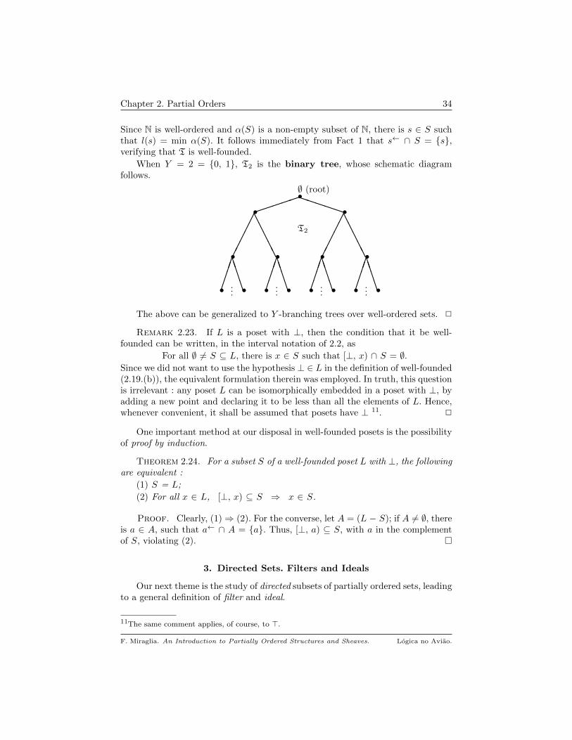
When Y = 2 = 0, 1, T2 is the binary tree, whose schematic diagramfollows.
• • • • • • • •
• • • •
• ••∅ (root)
BBBB
BBBB
BBBB
BBBB
AAAAA
AAAAA
PPPP
P
T2
......
......
The above can be generalized to Y -branching trees over well-ordered sets. 2
Remark 2.23. If L is a poset with ⊥, then the condition that it be well-founded can be written, in the interval notation of 2.2, as
For all ∅ 6= S ⊆ L, there is x ∈ S such that [⊥, x) ∩ S = ∅.Since we did not want to use the hypothesis ⊥ ∈ L in the definition of well-founded(2.19.(b)), the equivalent formulation therein was employed. In truth, this questionis irrelevant : any poset L can be isomorphically embedded in a poset with ⊥, byadding a new point and declaring it to be less than all the elements of L. Hence,whenever convenient, it shall be assumed that posets have ⊥ 11. 2
One important method at our disposal in well-founded posets is the possibilityof proof by induction.
Theorem 2.24. For a subset S of a well-founded poset L with ⊥, the followingare equivalent :
(1) S = L;
(2) For all x ∈ L, [⊥, x) ⊆ S ⇒ x ∈ S.
Proof. Clearly, (1)⇒ (2). For the converse, let A = (L − S); if A 6= ∅, thereis a ∈ A, such that a← ∩ A = a. Thus, [⊥, a) ⊆ S, with a in the complementof S, violating (2).
3. Directed Sets. Filters and Ideals
Our next theme is the study of directed subsets of partially ordered sets, leadingto a general definition of filter and ideal.
11The same comment applies, of course, to >.
F. Miraglia. An Introduction to Partially Ordered Structures and Sheaves. Logica no Aviao.
Chapter 2. Partial Orders 35
Definition 2.25. Let S be a subset of a poset L.
a) S is up directed if
[ud] For all a, b ∈ S, there is c ∈ S such that a ≤ c and b ≤ c.
The concept of down directed is dual, that is,
[dd] For all a, b ∈ S, there is c ∈ S such that c ≤ a and c ≤ b.
We abbreviate up directed by ud and down directed by dd. Some authors use right(left) directed for ud (resp., dd) sets.
b) S is up cofinal (ucof) in L if
[ucof ] For all a ∈ L, there is c ∈ S such that a ≤ c.
c) S is down cofinal (dcof) if
[dcof ] For all a ∈ L, there is c ∈ S such that c ≤ a.
d) S is cofinal if it is up and down cofinal.
The notion of directed set is instrumental to construct the concepts of filterand ideal in a poset.
Definition 2.26. Let S be a subset of a poset L.
a) S is a filter in L if S 6= ∅ and the following hold :
[Fi1] : S is dd in L;
[Fi2] : ∀ a, b ∈ L, (a ∈ S and a ≤ b ⇒ b ∈ S).
For a ∈ L, a→ is the principal filter generated by a in L.
b) S is an ideal in L if S 6= ∅ and the following hold :
[Id1] : S is ud in L;
[Id2] : ∀ a, b ∈ L (a ∈ S and b ≤ a ⇒ b ∈ S).
If a ∈ L, a← is the principal ideal generated by a in L.
A filter or ideal is said to be proper if it is distinct from L.
Clearly, Definitions 2.25 and 2.26 presents a set of pairs of dual concepts.Notice that a filter is down directed upper set, while an ideal is a ud lower set. Infact, some authors call a dd set a filter base and a ud set an ideal base. Thereason is the following result, whose proof is left to the reader.
Lemma 2.27. With notation as in 2.7, the following conditions are equivalent,for a subset S of a poset L :
(1) S is dd (ud);
(2) S↑ is dd (resp., S↓ is ud);
(3) S↑ is a filter (resp., S↓ is an ideal).
Example 2.28. Let X be a set and (2X , ⊆) be the power set of X, partiallyordered by inclusion. For S ⊆ 2X ,
a) S is ucof (dcof) iff X ∈ S (resp., ∅ ∈ S). This will always happen in a po with> (resp., ⊥).
b) The notions of filter and ideal in this po coincide with the usual ones in settheory 12 : S is a filter (ideal) in 2X iff
12We shall discuss filters and ideals in lattices in Chapter 3.
F. Miraglia. An Introduction to Partially Ordered Structures and Sheaves. Logica no Aviao.
Chapter 2. Partial Orders 36
(*) a, b ∈ S ⇒ a ∩ b ∈ S (resp., a ∪ b ∈ S);
(**) a ∈ S and a ⊆ b (resp., b ⊆ a) ⇒ b ∈ S. 2
Example 2.29. If X is a set, S ⊆ 2X and x ∈ X, define
Sx = U ∈ S : x ∈ U.Let L = 2X − ∅, partially ordered by ⊆. For S ⊆ L we have :
a) S is dcof or left cofinal in L iff ∀ x ∈ X, x ∈ Sx.
b) S is a filter in L iff S is a filter in 2X , such that ∅ 6∈ S (i.e., S is a properfilter).
c) S is an ideal in L iff S ∪ ∅ is an ideal in 2X . 2
Example 2.30. Let T be a topological space and L = Ω(T ) − ∅, the nonempty open sets of T , partially ordered by ⊆. With notation as in Example 2.29,and for S ⊆ L, we have :
a) S is dcof or left cofinal in L iff ∀ t ∈ T , St is a neighborhood basis of t inT . In particular,
⋃S is a dense open in T . Conversely, if V is a dense open in T ,
then S = Ω(V ) − ∅ is dcof in L.
b) S is a filter (ideal) in Ω(T ) iff it satisfies conditions (*) and (**) of 2.28 above,relative to Ω(T ). The concepts of filter/ideal in L correspond to that of properfilter/ideal in Ω(T ). 2
Example 2.31. Let L = pF (X,Y ), partially ordered by the extension po, asin 2.12.
a) Left cofinal subsets of L are not very interesting. On the other hand, ucof orright cofinal subsets furnish ‘samples’ of the possible values of elements in L. Theset
D(x) = f ∈ L : x ∈ domfis clearly up cofinal in L. As another example, fix g ∈ L and consider
D(g) = f ∈ L : f ≥ g or x ∈ X : fx 6= gx 6= ∅.Simple calculations will show that D(g) is up cofinal in L.
b) A subset S ⊆ L is a proper filter iff
i) ∅ ∈ S;
ii) S contains all extensions of its members;
iii) ∀ f , g ∈ S, x ∈ X : fx = gx 6= ∅.c) S is an ideal in L iff S consists of a family of pairwise compatible maps,together with the ‘gluing’ of every finite subset of S and all restrictions of elementsof S to subsets of their domains. Thus, S is an ideal iff :
∗ ∀ f , g ∈ S, f|domf∩domg = f|domf∩ domgand f ∨ g ∈ S;
∗ ∀ f ∈ S, ∀ A ⊆ domf , f|A ∈ S.
For a non-empty S ⊆ L, the following are equivalent :(a)
∨S exists in L; (b) S is bounded in L;
(c) S is contained in some ud set T ; (d) S is contained in some ideal I.
F. Miraglia. An Introduction to Partially Ordered Structures and Sheaves. Logica no Aviao.
Chapter 2. Partial Orders 37
If the above equivalent conditions hold, then the ud subset T and the ideal I canbe chosen so that
∨S =
∨T =
∨I. Hence, in pF (X,Y ), every non-empty ud
subset has a supremum.
By Lemma 1.2, an ideal S in L furnishes a function∨S ∈ L; the domain of∨
S might be very small (∅ is an ideal). One way to guarantee that dom∨S
= X is to require that for all ucof H ⊆ L, we have S ∩ H 6= ∅. Such ideals areusually called generic.
In expositions of forcing in set theory, it is the reverse order of the one abovethat is used (see, for instance, [40]). We are then led to consider filters, dcof (ordense) subsets and generic filters. 2
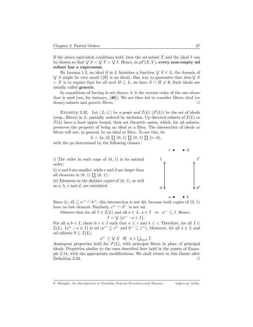
Example 2.32. Let 〈L,≤〉 be a poset and I(L) (F(L)) be the set of ideals(resp., filters) in L, partially ordered by inclusion. Up directed subsets of I(L) orF(L) have a least upper bound, their set theoretic union, which, for ud subsets,preserves the property of being an ideal or a filter. The intersection of ideals orfilters will not, in general, be an ideal or filter. To see this, let
L = a, b∐
(0, 1)∐
(0, 1)∐c, d,
with the po determined by the following clauses :
i) The order in each copy of (0, 1) is its naturalorder;
ii) a and b are smaller, while c and d are larger thanall elements in (0, 1)
∐(0, 1);
iii) Elements in the distinct copies of (0, 1), as wellas a, b, c and d, are unrelated.
•a • b
b
b
0
1
b
b
0′
1′
•c • d
Since c, d ⊆ a→ ∩ b→, this intersection is not dd, because both copies of (0, 1)have no last element. Similarly, c← ∩ d← is not ud.
Observe that for all I ∈ I(L) and all a ∈ L, a ∈ I ⇔ a← ⊆ I. Hence,
I =∨a← : a ∈ I.
For all a, b ∈ I, there is c ∈ I such that a ≤ c and b ≤ c. Therefore, for all I ∈I(L), a← : a ∈ I is ud (a← ⊆ c← and b← ⊆ c←). Moreover, for all a ∈ L andud subsets S ⊆ I(L),
a← ≤∨S iff a ∈
⋃I∈S I.
Analogous properties hold for F(L), with principal filters in place of principalideals. Properties similar to the ones described here hold in the posets of Exam-ple 2.14, with the appropriate modifications. We shall return to this theme afterDefinition 2.43. 2
F. Miraglia. An Introduction to Partially Ordered Structures and Sheaves. Logica no Aviao.

Chapter 2. Partial Orders 38
4. The Countable Chain Condition
Definition 2.33. Let 〈L,≤〉 be a poset and a, b ∈ L.
∗ a and b are up-compatible (compatible) if a→ ∩ b→ ∩ L− 6= ∅(resp., a← ∩ b← ∩ L− 6= ∅) 13.
∗ a and b are up-incompatible (resp., incompatible), writtena ⊥∗ b (resp., a ⊥ b) if they are not up-compatible (resp., compatible).
L is up-ccc (ccc) (countable chain condition) iff every set of pairwise up-incompatible (resp., incompatible) elements is at most countable. Hence, ≤ is upccc iff ≤op is ccc and vice-versa.
Remark 2.34. Terminology here is not quite standard. There is always thequestion of duality and of what is the “natural” way in which “increasing” or“decreasing” are understood. The examples below will help, hopefully, to makematters clearer. 2
Example 2.35. If T is a topological space and L = Ω(T ) with the inclusionpo, then :
i) U ⊥∗ V iff U ∪ V = T .
ii) U ⊥ V iff U ∩ V = ∅.Hence, our notion of ccc corresponds to what is known in the literature as a ccctopological space : any set of pairwise disjoint opens is at most countable. 2
Example 2.36. If L = pF (X,Y ), with the extension partial order of 2.12,then :
a) f ⊥∗ g iff they do not have a common extension
iff x ∈ X : fx 6= gx 6= ∅;b) f ⊥ g iff x ∈ X : fx = gx = ∅.
In the literature in Set Theory, sub posets of pF (X,Y ) are said to be ccc ifthey are up-ccc in our terminology. 2
Remark 2.37. If α is a cardinal, it should be clear how to define the conceptof α-ccc (the α chain condition). As above we would have a pair of dual up/down(or left/right) conditions. 2
Theorem 2.39 below, of independent interest, will guarantee that certain posetsare ccc. From here on, we assume that the well-ordering axiom (WOA) in 2.23 ispart of the axioms of Set Theory. We first recall the concept of regular cardinal.
Definition 2.38. Let K be a set. card(K) is regular if it is infinite and forall Ai : i ∈ I ⊆ 2K ,
card(I) < card(K)
and
card(Ai) < card(K), ∀ i ∈ I⇒ card(
⋃i∈I Ai) < card(K).
13Recall from 2.1 that L− = L − ⊥, >.
F. Miraglia. An Introduction to Partially Ordered Structures and Sheaves. Logica no Aviao.

Chapter 2. Partial Orders 39
Theorem 2.39. (Erdos-Rado) Let A be a set, n ≥ 1 a positive integer andK an infinite collection of subsets of A of cardinality n. Assume that card(K) isregular. Then there is a B ⊆f A and K ′ ⊆ K such that
(1) card(K) = card(K ′); (2) For all α, β ∈ K ′, α ∩ β = B.
Proof. By induction on n ≥ 1. If n = 1, then either
∗ There is a ∈ K that is common to card(K) elements of K; in this case, set B =a;∗ No such element exists and set B = ∅.
Suppose the result true for (n−1) ≥ 1 and that the elements of K have cardinaln. Assume A is well ordered and for α ∈ K, let aα be the least element of α inthis order. Consider the set
C = α − aα : α ∈ K.There are two possibilities :
1. card(C) < card(K) : For u ∈ C, define
Ku = α ∈ K : α − aα = u.Then K =
⋃Ku : u ∈ C; since card(K) is regular (2.38) and card(C) < card(K),
there is B ∈ C such that card(KB) = card(K). Now observe that for all α, β ∈KB , α ∩ β = B.
2. card(C) = card(K) : Since the elements of C have cardinal (n−1), by induction
there is D ⊆f A and C ′ ⊆ C, with card(C ′) = card(C) = card(K) and U ∩ V =D, ∀ U , V ∈ C ′. Consider the cardinality of
T = aα : α − aα ∈ C ′.Again there are two possibilities :
card(T ) < card(K) : For a ∈ T , let Ka = β : (β − a) ∈ C ′; clearly,⋃Ka : a ∈ T has cardinality equal to card(K) (it is larger than or equal
to card(C ′)). Since card(T ) is strictly less the regular card(K), there is a ∈ T suchthat card(Ka) = card(K). It is straightforward to check that for all β, γ in Ka,β ∩ γ = D ∪ a.card(T ) = card(K) : For a ∈ T , select α ∈ K with (α − a) ∈ C ′. It is clear
that this selection produces a subset K ′ ⊆ K such that for all α, β ∈ K ′, we haveα ∩ β = D, ending the proof
Corollary 2.40. Let A be a set and K an uncountable collection of finitesubsets of A. Then there is B ⊆f A and an uncountable K ′ ⊆ K such that ∀ α,β ∈ K ′, α ∩ β = B. If card(K) is regular, then there is K ′ ⊆ K with the aboveproperty, with card(K ′) = card(K).
Proof. For each n ≥ 1, let Kn = α ∈ K : card(α) = n; then K =⋃Kn
and so, being uncountable, at least one of the Kn must be uncountable. If card(K)is regular, then card(Kn) = card(K), for some n ≥ 1. If card(K) is not regular,one can always choose a regular uncountable cardinal below card(K) 14. The fullstatement of the Corollary now follows from 2.39.
14The first uncountable cardinal, ω1, is regular.
F. Miraglia. An Introduction to Partially Ordered Structures and Sheaves. Logica no Aviao.
Chapter 2. Partial Orders 40
Remark 2.41. Although Theorem 2.39 is true if card(K) is countable (aregular cardinal), this is not the case of Corollary 2.40. It is not very hard to findexamples of this. 2
As an application of these results, we show that the posets pFω(X,Y ) (2.13)are up-ccc, if Y is finite.
Corollary 2.42. If X, Y are sets, then pFω(X,Y ) is up-ccc in the extensionpo, whenever Y is finite.
Proof. Write Z = pFω(X,Y ) and suppose T is an uncountable set of up-incompatible elements in Z. Since for finite D, Y D is finite, K = dom t : t ∈ Tis uncountable. By Corollary 2.40, there is B ⊆f X and an uncountable K ′ ⊆ Ksuch that u ∩ v = B, for all u, v ∈ K ′. Let T ′ = t ∈ T : dom t ∈ K ′; if s, t ∈ T ′,then 2.36.(a) implies that s|B 6= t|B , because s ⊥∗ t. But this is impossible, since
T ′ is uncountable and Y B is finite.
We shall apply 2.42 in 18.6 to show that all dyadic spaces are ccc. Moreinformation on combinatorics and chain conditions can be found in [40] and [9].
5. Continuous and Algebraic Posets. Compactness
Analogy with topology produces the following
Definition 2.43. Let 〈L,≤〉 be a poset, a, b ∈ L and S ⊆ L.
a) a is compact (also algebraic or finite) in L iff for all ud S ⊆ L,
S→ ⊆ a→ ⇒ There is s ∈ S such that a ≤ s.
For b ∈ L, set cp(b) = a ∈ L : a is compact and a ≤ b.b) a is way below b, in symbols a b, iff for all ud S ⊆ L,
S→ ⊆ b→ ⇒ There is s ∈ S such that a ≤ s.
For b in L, set b←← = a ∈ L : a b.Note that a is compact iff a a.
c) ≤ is a continuous po on L (or L is a continuous poset) iff
[cpo1] : All non-empty, up directed subsets of L, have a sup in L;
[cpo2] : For all a in L, a←← is up directed and a =∨a←←.
d) L is an algebraic poset iff it is a continuous poset such that for all a ∈ L,cp(a) is up directed and a =
∨cp(a).
e) A poset with > is compact if it is algebraic and > is compact.
One can find much information on this topic in [17], where its connections withlattice theory, computer science, general topology, analysis, C∗-algebras and Topostheory are presented and explored. The material in [34] is also interesting, with adifferent point of view. Here we will be content with discussing the above propertiesrelative to the examples already given and presenting another two, important forfuture work.
F. Miraglia. An Introduction to Partially Ordered Structures and Sheaves. Logica no Aviao.
Chapter 2. Partial Orders 41
Remark 2.44. Our definition of compact and “way below” is not that in[17] since we wanted to state it without the assumption of “completeness”. Thefollowing observations are, therefore, in order :
a) Since the sets S in the definition of the way below relation are ud, we have 15
a b ⇔ ∀ ud S ⊆ L, S→ ⊆ a→ ⇒ ∃ F ⊆f S, with F→ ⊆ a→.
Similarly for the notion of compactness. This is closer to the usual topologicaldefinition of compactness.
b) In the presence of [cpo1] we may rewrite the definition of a b as :
∀ ud S ⊆ L, b ≤∨S ⇒ ∃ s ∈ S (a ≤ s).
Similarly for the concept of compactness.
c) If L has sups for all finite subsets (or equivalently, for each pair of its elements),then
a b iff ∀ S ⊆ L, S→ ⊆ a→ ⇒ ∃ F ⊆f S with a ≤∨F .
This holds because, in this case, given S ⊆ L, we can form
S′ = sup F : F ⊆ S and F is finite,which is ud and satisfies S→ = (S′)→. Similarly, of course, for compactness.
d) If L has sups for all its subsets then
a b iff ∀ S ⊆ L, b ≤∨S ⇒ ∃ F ⊆f S, with a ≤
∨F . 2
Proposition 2.45. In a poset 〈L,≤〉 the relation has the following prop-erties : for x, y, u, z ∈ La) x y ⇒ x ≤ y.
b) u ≤ x y ≤ z ⇒ u z. If x is compact and z ≤ x ≤ y, then z x y.
c) If L has finite sups then :
(i) x z, y z ⇒ supx, y z. In particular, z←← is ud.
(ii) If x and y are compact, so is x ∨ y. In particular, cp(z) is ud.
Proof. For item (a), just consider the ud set a. The remaining assertionsfollow straightforwardly from the definitions.
We now relate the notion of algebraic compactness with its topological version,presented in Definition 1.23.
Proposition 2.46. Let T be a topological space and V , U ∈ Ω(T ).
a) In 〈Ω(T ),⊆〉, consider the following conditions :
(1) V U ; (2) V is relatively compact (1.23) in U .
Then, (2) ⇒ (1). If T is regular (1.20), these conditions are equivalent.
b) U is compact in the poset 〈Ω(T ),⊆〉 iff it is (topologically) compact.
c) Consider the following conditions :
(1) 〈Ω(T ),⊆〉 is a continuous poset;
(2) Every open set in T is the union of relatively compact opens in U .
(3) T is locally compact, i.e., for U ∈ Ω(T ) and x ∈ U ,
15⊆f means “finite subset of”, defined in page 15.
F. Miraglia. An Introduction to Partially Ordered Structures and Sheaves. Logica no Aviao.

Chapter 2. Partial Orders 42
[lc] There is V ∈ νx 16 such that V ⊆ U and V is compact.
Then (3) ⇒ (2) ⇒ (1). If T is regular, these conditions are equivalent.
d) The following are equivalent :
(1) 〈Ω(T ),⊆〉 is an algebraic poset;
(2) T has a basis of compact opens, that is, every open in T is the union ofcompact opens.
Proof. Recall that Ω(T ) has arbitrary sups and so we may use the displayedstatement in 2.44.(d) as the definition of in Ω(T ). We discuss (a), leaving theother items to the reader.
a) For V ⊆ U , assume that V ∩ U is compact in U (or, equivalently, in T ;see 1.24.(b)). If S ⊆ Ω(U) is a covering of U , then there is C ⊆f S such that
V ⊆ V ∩ U ⊆⋃C, and V U , establishing that (2) ⇒ (1).
To show that (1) ⇒ (2), suppose that T is regular and let S ⊆ Ω(U) be anopen covering of F = V ∩ U . The covering S is refined in two ways :
∗ By Lemma 1.21.(b), eachW ∈ S may be written as a union of opens whose closureis contained in W ; let S′ be the covering of F obtained through the refinement ofS by this method;
∗ Let S′′ = S′ ∪ V c ∩ U.Since V
c ∩ U is the complement of F in U – it is clearly open –, S′′ is an opencovering of U . It follows from (1) that there is B ⊆f S′′, such that V ⊆
⋃B. Since
Vc ∩ U has empty intersection with V , we may as well assume that it is not in
B. Since closure commutes with finite unions (1.10.(d)), we get
F ⊆⋃W∈B W . (*)
Now, for each W ∈ B, select A ∈ S such that W ⊆ A. Because B is finite, oneobtains a finite subset of S that, by (*), is a covering of F , ending the proof.
Example 2.47. In 2X , a set is compact iff it is finite. Again, we have acontinuous poset, which is algebraic.
In pF (X,Y ), an element is compact iff its domain is finite; it is easily verifiedthat pF (X,Y ) is an algebraic poset. 2
Example 2.48. An important example of a continuous poset which is notalgebraic is the real unit interval [0, 1], with its usual order. We have a biff a < b or a = 0. On the other hand, the only compact element of [0, 1] is 0.Another example of this sort (but harder to verify), is furnished by LSC(T ), thelower semicontinuous functions on a compact space T . 2
Example 2.49. Let A be an algebra in the sense of universal algebra, i. e.,A is a set, together with a set of n-ary operations on A, for each n ≥ 0.
If A is an algebra, a congruence θ on A is an equivalence relation such thatfor all n ≥ 1, all n-ary operations α on A and all 〈 a1, . . . , an 〉, 〈 b1, . . . , bn 〉 in An,
ai θ bi, 1 ≤ i ≤ n, ⇒ α(a1, . . . , an) θ α(b1, . . . , bn).
16The filter of opens neighborhoods of x in T ; see section 1.2.
F. Miraglia. An Introduction to Partially Ordered Structures and Sheaves. Logica no Aviao.

Chapter 2. Partial Orders 43
Let Con(A) be the set of congruences on A. With the containment po inheritedfrom A2, Con(A) is a poset. Clearly, Con(A) is closed under arbitrary intersections.Thus, every subset S ⊆ A × A generates a congruence on A, given by
θS =⋂θ ∈ Con(A) : S ⊆ θ,
the smallest congruence relation containing S. Note that the equality relation (thediagonal of A × A) is the ⊥ of Con(A), while A × A is its >. Hence, in Con(A)all subsets have sup and inf.
For each 〈x, y 〉 in A × A, let θxy be the congruence generated by 〈x, y 〉.Clearly, θxy = θyx. Note that θxy is compact in Con(A) and for all θ in Con(A)
θ =∨θxy : 〈x, y 〉 ∈ θ.
Thus, Con(A) is an algebraic lattice. This example has many interesting instances:groups, rings, etc. 2
Exercises
2.50. a) If L is a poset, show that I(L) and F(L) (2.32) are continuousalgebraic posets.
b) If M is a module over a commutative ring, show that the lattice of submodulesof M (2.14) is an algebraic poset. 2
2.51. Let I be a set and [0, 1] be the real unit interval. In the power [0, 1]I ,with the coordinate-wise order (2.16), show that 17
(xi) (yi) iff
∀ i ∈ I, xi yi
and
∃ F ⊆f I with xi = 0 if i ∈ (I − F ). 2
2.52. One of the basic examples of poset is the family of subsets of a set,2X , partially ordered by inclusion. We can produce further posets by consideringsubsets S ⊆ 2X , with the induced order. Show that this, in fact, produces allposets, except for isomorphism. 2
17Recall that ⊆f denotes “finite subset of”.
F. Miraglia. An Introduction to Partially Ordered Structures and Sheaves. Logica no Aviao.
CHAPTER 3
Lattices
Recall that A ⊆f B means that A is a finite subset of B (page 15).
Definition 3.1. Let (L,≤) be a poset.
a) L is a semilattice iff for all F ⊆f L,∧F exists in L. When F = x, y,
write x ∧ y for inf x, y 1. Thus, all semilattices have > =∧∅.
b) L is a join semilattice iff for all F ⊆f L,∨F exists in L; for x, y ∈ L,
x ∨ y indicates sup x, y 2. Note that all join semilattices have ⊥ =∨∅.
c) L is a lattice iff for all F ⊆f L, both∧F and
∨F exist in L. Hence, all
lattices have ⊥ and >.
If L and P are lattices, a morphism, f : L −→ P , is a map such that for allF ⊆f L
f(∨F ) =
∨f(F ) and f(
∧F ) =
∧f(F ),
where, as usual, f(F ) = fx : x ∈ F.d) A sublattice of L is a subset P of L, such that for all F ⊆f P ,
∨F and
∧F ,
computed in L, are in P . Thus,∨
F and∧
F in P exist, and are identical tothe sup and inf taken in L.
Note that the canonical injection P −→ L is a morphism iff P is a sublatticeof L.
Lattices and their morphisms are a category, denoted by L. We write L ∈ Ob(L)and f ∈ M(L) to indicate that L is a lattice and that f is a lattice morphism.
Standard references on lattices are [21], [5] and [3]; [60] is also very interesting.In general, the definitions will allow for the absence of ⊥ and/or >. It is simple tomodify the above to cover that : just require that non-empty finite sets have infand/or sup. We will be mainly interested in lattices with ⊥ and >. The followingis straightforward :
Lemma 3.2. Let Lf−→ P be a map between lattices.
a) f is a morphism iff it verifies
∗ f(⊥) = ⊥ and f(>) = >;
∗ ∀ x, y ∈ L, f(x ∨ y) = fx ∨ fy and f(x ∧ y) = fx ∧ fy.
b) If f is a morphism, then f is increasing (i.e., a poset morphism) and the imageof f is a sublattice of P .
1Also called the meet of x and y.2Also called the join of x and y.
44
Chapter 3. Lattices 45
c) If f is increasing, then it is a lattice morphism iff
∗ f(⊥) = ⊥ and f(>) = >;
∗ ∀ x, y ∈ L, f(x ∨ y) ≤ fx ∨ fy and fx ∧ fy ≤ f(x ∧ y).
Many of the examples in Chapter 2 are lattices : 2Xλ and Bλ(X) (2.9), linearorders, the opens of a topological space (2.11), congruences on an algebra (2.49)and the posets presented in 2.14. We also have examples of semilattices and joinsemilattices.
Example 3.3. If Li, i ∈ I, is a family of lattices, the set-theoretical product,∏Li, has a natural lattice structure, where the operations of ∧ and ∨ are defined
coordinatewise :
∀ i ∈ I, [s ∧ t](i) = s(i) ∧ t(i) and [s ∨ t](i) = s(i) ∨ t(i).Note that > and ⊥ in
∏Li are the constant sequences > and ⊥, respectively. The
canonical projections∏Li
πi−→ Li are lattice morphisms.
If f : D −→ L is a lattice morphism, define
D ×f D = 〈 a, b 〉 ∈ D × D : fa = fb.With the operations induced by D × D, D ×f D is a lattice, called the fiberedproduct of D over f . The restriction of the canonical projections π1, π2 fromD × D to D are lattice morphisms, still indicated by πi, i = 1, 2. Note thatf π1 = f π2. This construction yields a proof that monomorphisms in thecategory L are precisely the injective lattice morphisms (Exercise 3.15.(d)). 2
Example 3.4. We shall now construct the coproduct of a family of lattices,Li : i ∈ I, written
∐i∈I Li. The question here is to obtain a lattice with ⊥ and
>. The formal definition of coproduct of a family of object in a category appearsin Example 16.30.(b), while that of initial object in a category in Definition 16.9.
If I = ∅, set ∐i∈I Li =def 2 = ⊥, >,
where 2 is the two-element lattice with ⊥ < >. Note that for all lattices L, thereis a unique lattice morphism from 2 to L, taking ⊥ to ⊥ and > to >. Hence, 2 isthe initial object in the category of lattices 3.
From here on assume that I 6= ∅ and let
T = s ∈∏Li : i ∈ I : si 6= > is finite,
with the partial order induced by∏Li. Define
B = s ∈ T : i ∈ I : si = ⊥ 6= ∅.Now note that :
(1) B is closed under meets;
(2) T = B ∪⋃s∈T−B s, and this union is disjoint.
Hence, there is a unique equivalence relation θ on T , whose equivalence classes areprecisely B and, for s ∈ T − B, the singleton s. Whence, for s, t ∈ T , s θ t
iff s, t ∈ B or s, t ∈ T − B and s = t.
Set
3It is a general fact that an empty coproduct, if it exists, is an initial object.
F. Miraglia. An Introduction to Partially Ordered Structures and Sheaves. Logica no Aviao.
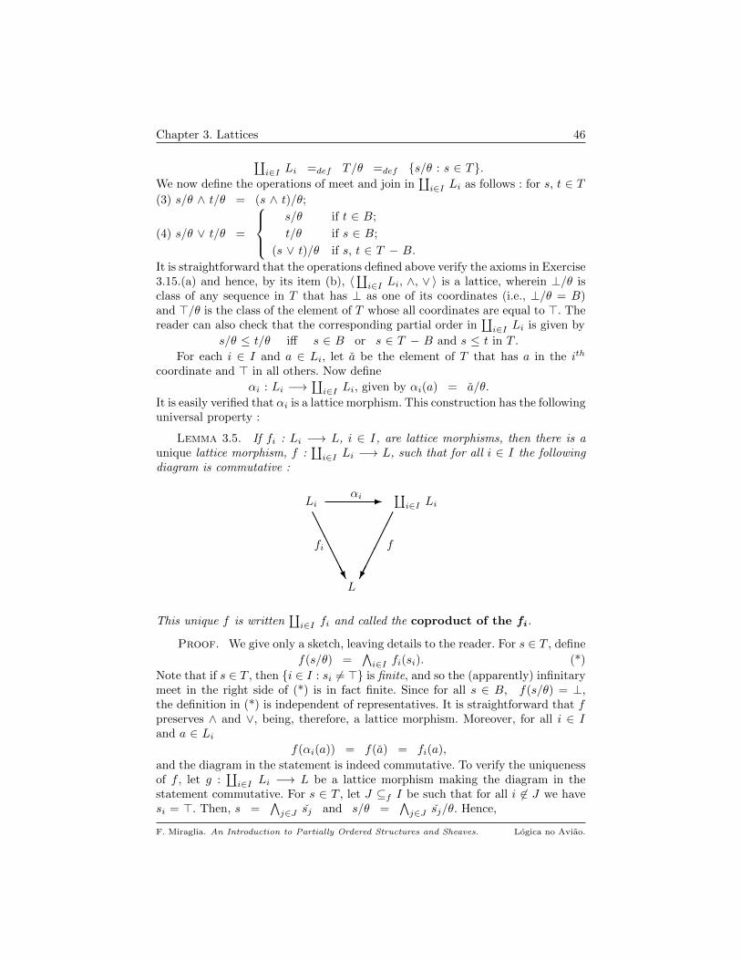
Chapter 3. Lattices 46
∐i∈I Li =def T/θ =def s/θ : s ∈ T.
We now define the operations of meet and join in∐i∈I Li as follows : for s, t ∈ T
(3) s/θ ∧ t/θ = (s ∧ t)/θ;
(4) s/θ ∨ t/θ =
s/θ if t ∈ B;
t/θ if s ∈ B;
(s ∨ t)/θ if s, t ∈ T − B.
It is straightforward that the operations defined above verify the axioms in Exercise3.15.(a) and hence, by its item (b), 〈
∐i∈I Li, ∧, ∨ 〉 is a lattice, wherein ⊥/θ is
class of any sequence in T that has ⊥ as one of its coordinates (i.e., ⊥/θ = B)and >/θ is the class of the element of T whose all coordinates are equal to >. Thereader can also check that the corresponding partial order in
∐i∈I Li is given by
s/θ ≤ t/θ iff s ∈ B or s ∈ T − B and s ≤ t in T .
For each i ∈ I and a ∈ Li, let a be the element of T that has a in the ith
coordinate and > in all others. Now define
αi : Li −→∐i∈I Li, given by αi(a) = a/θ.
It is easily verified that αi is a lattice morphism. This construction has the followinguniversal property :
Lemma 3.5. If fi : Li −→ L, i ∈ I, are lattice morphisms, then there is aunique lattice morphism, f :
∐i∈I Li −→ L, such that for all i ∈ I the following
diagram is commutative :
Li - ∐i∈I Li
fi f
L
αi
AAAAAAU
This unique f is written∐i∈I fi and called the coproduct of the fi.
Proof. We give only a sketch, leaving details to the reader. For s ∈ T , define
f(s/θ) =∧i∈I fi(si). (*)
Note that if s ∈ T , then i ∈ I : si 6= > is finite, and so the (apparently) infinitarymeet in the right side of (*) is in fact finite. Since for all s ∈ B, f(s/θ) = ⊥,the definition in (*) is independent of representatives. It is straightforward that fpreserves ∧ and ∨, being, therefore, a lattice morphism. Moreover, for all i ∈ Iand a ∈ Li
f(αi(a)) = f(a) = fi(a),
and the diagram in the statement is indeed commutative. To verify the uniquenessof f , let g :
∐i∈I Li −→ L be a lattice morphism making the diagram in the
statement commutative. For s ∈ T , let J ⊆f I be such that for all i 6∈ J we havesi = >. Then, s =
∧j∈J sj and s/θ =
∧j∈J sj/θ. Hence,
F. Miraglia. An Introduction to Partially Ordered Structures and Sheaves. Logica no Aviao.

Chapter 3. Lattices 47
g(s/θ) =∧j∈J g(sj) =
∧j∈J g(αj(sj)) =
∧j∈J fj(sj)
=∧i∈I fi(si) = f(s/θ),
ending the proof.
It is the universal property described by Lemma 3.5 that guarantees that thesystem 〈
∐i∈I Li, αi : i ∈ I 〉 is the coproduct of the Li in the category of
lattices, as stipulated by Definition 16.29 and Example 16.30.(b). 2
Example 3.6. Let T be a topological space. Recall from 1.11 that B(T ) andReg(T ) are the set of clopens and regular opens in T . We have (see [R] in page19)
∅, T ⊆ B(T ) ⊆ Reg(T ) ⊆ Ω(T )
as partially ordered sets. By 1.12,
B(T ) is a sublattice of Ω(T ).
It follows from 1.14 that Reg(T ) is a lattice with ⊥ = ∅, > = T and
U ∧ V = U ∩ V and U ∨ V = int (U ∪ V ).
However, Reg(T ) is not a sublattice of Ω(T ). 2
Recall from 2.49, that a congruence θ on a lattice L is an equivalence relationon L, such that for all x, y, a, b ∈ L,
x θ a and y θ b ⇒ (x ∧ y) θ (a ∧ b) and (x ∨ y) θ (a ∨ b).Write Con(L) for the lattice of congruences on L.
Example 3.7. Let Lf−→ P be a lattice morphism. For x, y ∈ L, define
x θf y iff fx = fy.
θf is a congruence on L, the congruence generated by f . 2
A congruence relation θ on L gives rise to a quotient L/θ, the set of equivalenceclasses of the elements of L by θ. For x ∈ L, write x/θ for the equivalence class ofx in L/θ. The following are straightforward :
a) ∀ x, y ∈ L, x θ (x ∧ y) iff y θ (x ∨ y). This allows us to define
x/θ ≤ y/θ iff x θ (x ∧ y),
yielding a partial order ≤ on L/θ.
b) The assignments,
x/θ ∨ y/θ = (x ∨ y)/θ and x/θ ∧ y/θ = (x ∧ y)/θ,
define operations on L/θ that, together with ⊥ = ⊥/θ and > = >/θ, make it thelattice associated to (L/θ,≤). Further, the map
πθ : L −→ L/θ, given by x 7→ x/θ
is a lattice morphism. The lattice L/θ is called the quotient of L by θ and πθ isthe quotient morphism.
Proposition 3.8. (Fundamental theorem for morphisms) Let L be a lattice,θ be a congruence on L and f : L −→ P be a lattice morphism. The followingconditions are equivalent :
F. Miraglia. An Introduction to Partially Ordered Structures and Sheaves. Logica no Aviao.
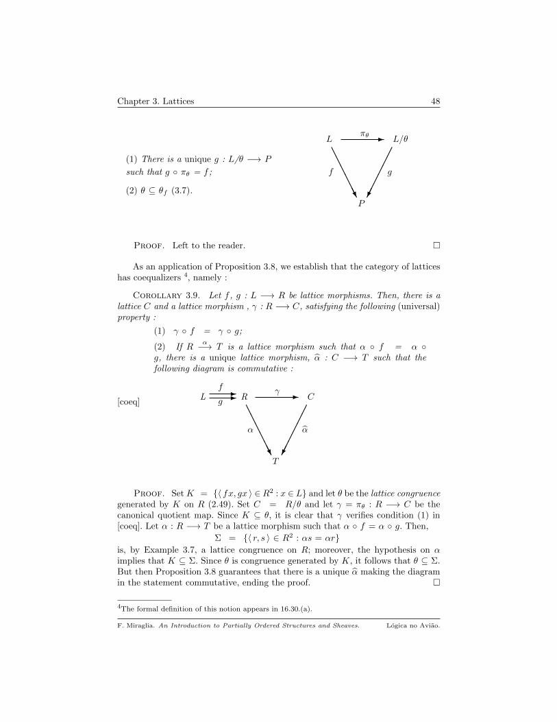
Chapter 3. Lattices 48
(1) There is a unique g : L/θ −→ P
such that g πθ = f ;
(2) θ ⊆ θf (3.7).
L - L/θ
f g
P
πθ
AAAAAAU
Proof. Left to the reader.
As an application of Proposition 3.8, we establish that the category of latticeshas coequalizers 4, namely :
Corollary 3.9. Let f , g : L −→ R be lattice morphisms. Then, there is alattice C and a lattice morphism , γ : R −→ C, satisfying the following (universal)property :
[coeq]
(1) γ f = γ g;
(2) If Rα−→ T is a lattice morphism such that α f = α
g, there is a unique lattice morphism, α : C −→ T such that thefollowing diagram is commutative :
L-f -
g R - C
α α
T
γ
AAAAAAU
Proof. Set K = 〈 fx, gx 〉 ∈ R2 : x ∈ L and let θ be the lattice congruencegenerated by K on R (2.49). Set C = R/θ and let γ = πθ : R −→ C be thecanonical quotient map. Since K ⊆ θ, it is clear that γ verifies condition (1) in[coeq]. Let α : R −→ T be a lattice morphism such that α f = α g. Then,
Σ = 〈 r, s 〉 ∈ R2 : αs = αris, by Example 3.7, a lattice congruence on R; moreover, the hypothesis on αimplies that K ⊆ Σ. Since θ is congruence generated by K, it follows that θ ⊆ Σ.But then Proposition 3.8 guarantees that there is a unique α making the diagramin the statement commutative, ending the proof.
4The formal definition of this notion appears in 16.30.(a).
F. Miraglia. An Introduction to Partially Ordered Structures and Sheaves. Logica no Aviao.
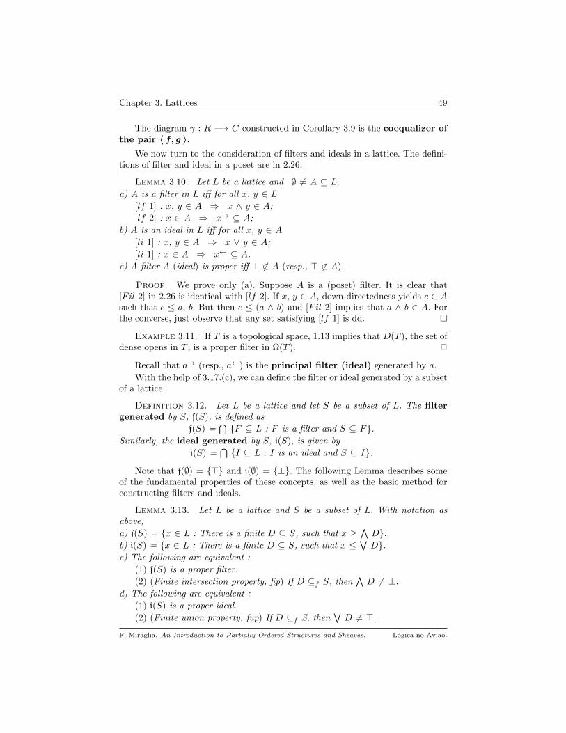
Chapter 3. Lattices 49
The diagram γ : R −→ C constructed in Corollary 3.9 is the coequalizer ofthe pair 〈 f, g 〉.
We now turn to the consideration of filters and ideals in a lattice. The defini-tions of filter and ideal in a poset are in 2.26.
Lemma 3.10. Let L be a lattice and ∅ 6= A ⊆ L.
a) A is a filter in L iff for all x, y ∈ L[lf 1] : x, y ∈ A ⇒ x ∧ y ∈ A;
[lf 2] : x ∈ A ⇒ x→ ⊆ A;
b) A is an ideal in L iff for all x, y ∈ A[li 1] : x, y ∈ A ⇒ x ∨ y ∈ A;
[li 1] : x ∈ A ⇒ x← ⊆ A.
c) A filter A (ideal) is proper iff ⊥ 6∈ A (resp., > 6∈ A).
Proof. We prove only (a). Suppose A is a (poset) filter. It is clear that[Fil 2] in 2.26 is identical with [lf 2]. If x, y ∈ A, down-directedness yields c ∈ Asuch that c ≤ a, b. But then c ≤ (a ∧ b) and [Fil 2] implies that a ∧ b ∈ A. Forthe converse, just observe that any set satisfying [lf 1] is dd.
Example 3.11. If T is a topological space, 1.13 implies that D(T ), the set ofdense opens in T , is a proper filter in Ω(T ). 2
Recall that a→ (resp., a←) is the principal filter (ideal) generated by a.
With the help of 3.17.(c), we can define the filter or ideal generated by a subsetof a lattice.
Definition 3.12. Let L be a lattice and let S be a subset of L. The filtergenerated by S, f(S), is defined as
f(S) =⋂F ⊆ L : F is a filter and S ⊆ F.
Similarly, the ideal generated by S, i(S), is given by
i(S) =⋂I ⊆ L : I is an ideal and S ⊆ I.
Note that f(∅) = > and i(∅) = ⊥. The following Lemma describes someof the fundamental properties of these concepts, as well as the basic method forconstructing filters and ideals.
Lemma 3.13. Let L be a lattice and S be a subset of L. With notation asabove,
a) f(S) = x ∈ L : There is a finite D ⊆ S, such that x ≥∧D.
b) i(S) = x ∈ L : There is a finite D ⊆ S, such that x ≤∨D.
c) The following are equivalent :
(1) f(S) is a proper filter.
(2) (Finite intersection property, fip) If D ⊆f S, then∧D 6= ⊥.
d) The following are equivalent :
(1) i(S) is a proper ideal.
(2) (Finite union property, fup) If D ⊆f S, then∨D 6= >.
F. Miraglia. An Introduction to Partially Ordered Structures and Sheaves. Logica no Aviao.
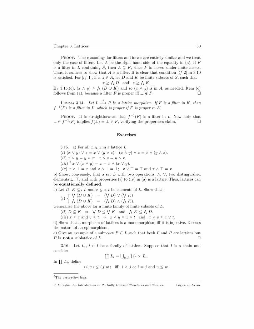
Chapter 3. Lattices 50
Proof. The reasonings for filters and ideals are entirely similar and we treatonly the case of filters. Let A be the right hand side of the equality in (a). If Fis a filter in L containing S, then A ⊆ F , since F is closed under finite meets.Thus, it suffices to show that A is a filter. It is clear that condition [lf 2] in 3.10is satisfied. For [lf 1], if x, z ∈ A, let D and K be finite subsets of S, such that
x ≥∧D and z ≥
∧K.
By 3.15.(c), (x ∧ y) ≥∧
(D ∪ K) and so (x ∧ y) is in A, as needed. Item (c)follows from (a), because a filter F is proper iff ⊥ 6∈ F .
Lemma 3.14. Let Lf−→ P be a lattice morphism. If F is a filter in K, then
f−1(F ) is a filter in L, which is proper if F is proper in K.
Proof. It is straightforward that f−1(F ) is a filter in L. Now note that⊥ ∈ f−1(F ) implies f(⊥) = ⊥ ∈ F , verifying the properness claim.
Exercises
3.15. a) For all x, y, z in a lattice L
(i) (x ∨ y) ∨ z = x ∨ (y ∨ z); (x ∧ y) ∧ z = x ∧ (y ∧ z).(ii) x ∨ y = y ∨ x; x ∧ y = y ∧ x.
(iii) 5 x ∨ (x ∧ y) = x = x ∧ (x ∨ y).
(iv) x ∨ ⊥ = x and x ∧ ⊥ = ⊥; x ∨ > = > and x ∧ > = x.
b) Show, conversely, that a set L with two operations, ∧, ∨, two distinguishedelements ⊥, >, and with properties (i) to (iv) in (a) is a lattice. Thus, lattices canbe equationally defined.
c) Let D, K ⊆f L and x, y, z, t be elements of L. Show that :
(i)
∨(D ∪ K) = (
∨D) ∨ (
∨K)∧
(D ∪ K) = (∧D) ∧ (
∧K).
Generalize the above for a finite family of finite subsets of L.
(ii) D ⊆ K ⇒∨D ≤
∨K and
∧K ≤
∧D.
(iii) x ≤ z and y ≤ t ⇒ x ∧ y ≤ z ∧ t and x ∨ y ≤ z ∨ t.d) Show that a morphism of lattices is a monomorphism iff it is injective. Discussthe nature of an epimorphism.
e) Give an example of a subposet P ⊆ L such that both L and P are lattices butP is not a sublattice of L. 2
3.16. Let Li, i ∈ I be a family of lattices. Suppose that I is a chain andconsider ∐
Li =⋃i∈I i × Li.
In∐Li, define
〈 i, u 〉 ≤ 〈 j, w 〉 iff i < j or i = j and u ≤ w.
5The absorption laws.
F. Miraglia. An Introduction to Partially Ordered Structures and Sheaves. Logica no Aviao.
Chapter 3. Lattices 51
The relation ≤ is a po. Is∐Li a lattice ? Is there an analogue of the morphisms
αi described in Example 3.4 for the direct sum ? 2
3.17. (Compare with 2.32) Let L be a poset.
a) If L is a semilattice, then the intersection of a family of filters in L is a filter.
b) If L is a join semilattice, the intersection of a family of ideals in L is an ideal.
c) If L is a lattice, the intersection of a family of filters (ideals) in L is a filter(resp., ideal).
d) If Ai, i ∈ I, is an upward directed (by inclusion) family of filters or ideals in L,then
⋃Ai is a filter or an ideal in L, respectively.
e) If L is a lattice, show that F(L) and I(L), the posets of filters and ideals in L,respectively, are lattices. 2
F. Miraglia. An Introduction to Partially Ordered Structures and Sheaves. Logica no Aviao.
CHAPTER 4
Distributive Lattices
We now come to the type of lattice that is central in all that follows.
Definition 4.1. A lattice L is distributive if it satisfies the following equiv-alent conditions :
[∧, ∨] : For all x, y, z ∈ L, x ∧ (y ∨ z) = (x ∧ y) ∨ (x ∧ z).
[∨, ∧] : For all x, y, z ∈ L, x ∨ (y ∧ z) = (x ∨ y) ∧ (x ∨ z).The notions of morphism and sublattice are the same as in the category of
lattices (3.1). In particular, Lf−→ P is an isomorphism iff there is P
g−→ Lsuch that f g = IdP and g f = IdL. If L and P are isomorphic we writeL ≈ P or L ≈f P , if there is need to display the isomorphism f explicitly.
Definition 4.1 and Exercise 3.15 guarantee that distributive lattices can beequationally defined.
Example 4.2. Except for the class of lattices in Example 2.10, all otherexamples in chapter 3 are distributive lattices. 2
Example 4.3. The lattices in 2.10 are important mathematical objects. Somesatisfy an alternative to distributivity, known as the modular law : ∀ x, y, z ∈ L
x ≤ z implies x ∨ (y ∧ z) = (x ∨ y) ∧ z.For closed subspaces of a Hilbert space, there is the operation of taking a
subspace to its orthogonal complement, x 7→ x⊥, satisfying :
(i) x ∧ x⊥ = ⊥; x ∨ x⊥ = >; (x⊥)⊥ = x.
(ii) (x ∧ y)⊥ = x⊥ ∨ y⊥.
(iii) (x ∨ y)⊥ = x⊥ ∧ y⊥.
(iv) (The orthomodular law) x ≤ y ⇒ x ∨ (x⊥ ∧ y) = y.
The interested reader may consult [5], [21] and [35]. 2
Distributive lattices and their morphisms form a category, denoted by D. Theexpressions L ∈ D and f ∈ M(D) indicate that L is a distributive lattice andthat f is a morphism in D.
Remark 4.4. There is a neat characterization of distributivity, due to Birkhoff,in terms of having or not certain finite lattices as sublattices. See, for instance,Theorem II.5.9, pg. 51 of [3]. 2
Example 4.5. The product (3.3) and the coproduct (3.4) of distributivelattices is distributive. Hence, 2 = ⊥, > is an initial object in the category D.
52
Chapter 4. Distributive Lattices 53
If f : L −→ P is a lattice morphism, with L distributive, then Im f is adistributive sublattice of P . 2
Example 4.6. If X is a topological space, the lattice of opens in X, Ω(X),is a distributive lattice, because it is a sublattice of 2X .
Let Y be a topological space and f : X −→Y be a continuous map. Definef∗ : Ω(Y ) −→ Ω(X) by U 7→ f−1(U). It is well known that f∗ preserves inter-sections and unions, being, therefore, a lattice morphism from Ω(Y ) to Ω(X). Ofcourse, if f is a homeomorphism, f∗ will be an isomorphism.
Recall from 3.6, that B(X), Reg(X) are the lattice of clopens and regularopens, respectively, in X. Since B(X) is a sublattice of Ω(X) it is also distributive.On the other hand, by 1.14.(f), Reg(X) is a distributive lattice, although not asublattice of Ω(X) or of 2X .
If we restrict f∗ to B(Y ), we get a lattice morphism from B(Y ) to B(X)(1.31.(a)). However, the inverse image of a regular open is not, in general, regular(1.31.(b)). For instance, for the sine function, sin : [0, π] −→ [0, 1], the inverseimage of (0, 1) is (0, π/2) ∪ (π/2, π), which is not regular.
There is a map f∗ : Ω(X) −→ Ω(Y ), closely associated to f∗. Define
f∗(V ) =⋃W ∈ Ω(Y ) : f∗(W ) ⊆ V .
f∗ is not direct image, as f might not be an open map. In fact,
f∗(V ) = int(Y − f(X − V )).
The connection between f∗ and f∗ is described by the adjunction :
(*) For all 〈V,W 〉 ∈ Ω(X) × Ω(Y ), f∗W ⊆ V iff W ⊆ f∗V .
A general way of obtaining such adjoint pairs is described in Theorem 7.8. 2
Lemma 4.7. Let L be a distributive lattice, a ∈ L, and S, T1, . . . , Tn be finitesubsets of L. Then,
a) a ∨ (∧S) =
∧a ∨ s : s ∈ S.
b) a ∧ (∨S) =
∨a ∧ s : s ∈ S.
c)∨ni=1 (
∧Ti) =
∧∨ni=1 f(i) : f ∈
∏Ti
d)∧ni=1 (
∧Ti) =
∨∧ni=1 f(i) : f ∈
∏Ti
Proof. Parts (a) and (b) come from the distributivity, by induction on thenumber of elements of S. Items (c) and (d) can be proven, for n = 2, by inductionon the number of elements of T1, the basis step being provided by (a) and (b).Finally, induction on n will finish the proof.
Remark 4.8. If L is a distributive lattice and θ is a lattice congruence on L,then the quotient lattice, L/θ, defined right before Proposition 3.8, is distributiveand called the quotient of L be θ. As before, πθ : L −→ L/θ is a lattice morphismand the statement of 3.8 is valid, ipsis litteris, for distributive lattices. In particular,Corollary 3.9 holds − with the same proof −, for distributive lattices, that is, inthis category every pair of morphisms has a coequalizer. 2
We now explore the relationship between congruences and filters or ideals ina distributive lattice.
F. Miraglia. An Introduction to Partially Ordered Structures and Sheaves. Logica no Aviao.
Chapter 4. Distributive Lattices 54
Definition 4.9. Let L be a distributive lattice and f : L −→ P be a latticemorphism.
a) If F ⊆ L is a filter in L, define, for x, y ∈ L,
x ∼F y iff there is z ∈ F such that x ∧ z = y ∧ z.
b) If I ⊆ L is an ideal in L, define, for x, y ∈ L,
x ∼I y iff there is z ∈ I such that x ∨ z = y ∨ z.
c) If θ is a congruence on L, set
Fθ = x ∈ L : x θ > and Iθ = x ∈ L : x θ ⊥.d) In the case θ is the congruence generated in L by f (3.7), the sets Fθ and Iθare called the cokernel and kernel of f , respectively :
coker f = x ∈ L : fx = > and ker f = x ∈ L : fx = ⊥.
Proposition 4.10. Let L be a distributive lattice.
a) For θ, θ′ ∈ Con(L), θ ⊆ θ′ ⇒ Fθ ⊆ Fθ′ and Iθ ⊆ Iθ′ .
b) If A is a filter or ideal in L, then ∼A is a congruence in L. Moreover,F∼A = A if A is a filter;
I∼A = A if A is an ideal.
c) For filters or ideals F , G in L, F ⊆ G iff ∼F ⊆ ∼G.
Proof. Item (a) is straightforward. In the remaining items, we treat onlythe case of filters; the proofs for ideals are analogous.
b) ∼A is an equivalence relation : Reflexivity and symmetry are immediate. Fortransitivity, let x, y, t ∈ L with x ∼A y and y ∼A t. Choose u and z in A such thatx ∧ u = y ∧ u and y ∧ z = t ∧ z. Since A is a filter, we have u ∧ z ∈ A, and so
x ∧ (u ∧ z) = (x ∧ u) ∧ z = (y ∧ u) ∧ z = (y ∧ z) ∧ u = (t ∧ z) ∧ u= t ∧ (u ∧ z),
showing that x ∼A t.
∼A is a congruence : Suppose x ∼A a and y ∼A b; let u, z be elements of A suchthat x ∧ u = a ∧ u and y ∧ z = b ∧ z. Then, u ∧ z ∈ A and we have
(u ∧ z) ∧ (x ∨ y) = (x ∧ u ∧ z) ∨ (y ∧ u ∧ z)= (a ∧ u ∧ z) ∨ (b ∧ u ∧ z)= (u ∧ z) ∧ (a ∨ b).
showing that (x ∨ y) ∼A (a ∨ b). Similar calculations, in fact not involving dis-tributivity, will verify that ∼A is a congruence with respect to ∧. For the displayedequation, note that
x ∈ F∼A iff x ∼A > iff for some z ∈ A, x ∧ z = > ∧ z = z
iff for some z ∈ A, x ≥ z.
Since A is a filter, we conclude that A = F∼A , as desired. Item (c) is a straight-forward consequence of (a) and (b).
4.11. Notation. If A is a filter or an ideal in a distributive lattice L, we adoptthe following notation, where x ∈ L :
∗ x/A is the equivalence class of x by the congruence ∼A;
F. Miraglia. An Introduction to Partially Ordered Structures and Sheaves. Logica no Aviao.

Chapter 4. Distributive Lattices 55
∗ L/A for the quotient lattice of L by the congruence ∼A;
∗ πA : L −→ L/A for the canonical quotient morphism. 2
Corollary 4.12. Let L be a distributive lattice and θ ∈ Con(L). With no-tation as in 4.9 and 4.11,
a) If A is a filter in L, then for all x, y ∈ Lx/A ≤ y/A iff ∃ z ∈ A such that x ∧ z ≤ y.
b) If A is an ideal in L, then for all x, y ∈ Lx/A ≤ y/A iff ∃ z ∈ A such that x ≤ y ∨ z.
c) Fθ is a filter and Iθ is an ideal in L. Furthermore, ∼Fθ ∪ ∼Iθ ⊆ θ.
d) The cokernel of a morphism is a filter and its kernel an ideal in L.
e) If A is a filter in L and θ ∈ Con(L), then ∼A ⊆ θ iff A ⊆ Fθ.
A corresponding statement holds for ideals.
Proof. We treat only the case of filters. For (a), note that if x, y ∈ L,
x/A ≤ y/A iff x/A ∧ y/A = (x ∧ y)/A = x/A iff (x ∧ y) ∼A x
iff ∃ z ∈ A such that x ∧ y ∧ z = x ∧ z.To conclude, note that the last equation is equivalent to (x ∧ z) ≤ y.
c) It is straightforward that Fθ and Iθ are, respectively, a filter and an ideal. Weshow that ∼Fθ ⊆ θ, leaving the analogous calculations for ∼Iθ to the reader. Forx, y ∈ L,
x ∼Fθ y iff ∃ z such that z θ > and x ∧ z = y ∧ z.From x θ x, y θ y and z θ >, we get (x ∧ z) θ x and (y ∧ z) θ y. Since x ∧ z= y ∧ z, transitivity yields x θ y, as required. Item (d) follows immediately from(c), while (e) is a consequence of 4.10 and (c).
For quotients by filters and ideals, Proposition 3.8 takes the following form,when the source of a morphism is distributive :
Corollary 4.13. Let L be a distributive lattice, F be a filter on L and
Lf−→ P be a lattice morphism. The following are equivalent:
(1) There is a unique g : L/F −→ P
such that g πF = f ;
(2) F ⊆ coker f .
L - L/F
g f
P
πF
AAAAAAU
A corresponding statement holds for ideals.
Proof. By Proposition 3.8, the existence of g is equivalent to ∼F ⊆ θf , while4.12.(e) implies that this condition is equivalent to F ⊆ Fθf = coker f .
Complementing Proposition 4.10, we prove
F. Miraglia. An Introduction to Partially Ordered Structures and Sheaves. Logica no Aviao.
Chapter 4. Distributive Lattices 56
Lemma 4.14. Let L be a lattice. With notation as in 4.9, the following areequivalent :
(1) L is a distributive lattice.
(2) For all filters A in L, the relation ∼A is a congruence in L.
(3) For all ideals A in L, the relation ∼A is a congruence in L.
(4) For all principal ideals A in L, ∼A is a congruence in L.
(5) For all principal filters A in L, ∼A is a congruence in L.
Proof. By 4.10, it is enough to verify that (5) ⇒ (1), i. e., if x, y, z ∈ L,then
x ∧ (y ∨ z) ≤ (x ∧ y) ∨ (x ∧ y). (I)
Let A = x→; since x ∧ y = x ∧ (x ∧ y), we have y ∼A x ∧ y; analogously,z ∼A x ∧ z. Since ∼A is a lattice congruence, we conclude that
(y ∨ z) ∼A [(x ∧ y) ∨ (x ∧ z)].Hence, there is t ∈ x→, such that
t ∧ (y ∨ z) = t ∧ [(x ∧ y) ∨ (x ∧ z)] ≤ (x ∧ y) ∨ (x ∧ z). (II)
But (II) and x ≤ t immediately imply (I), as desired.
Example 4.15. Let Li, i ∈ I, be a family of distributive lattices and F ⊆ 2I
be a filter in 2I (usually one says a filter on I). For s, t ∈∏Li, define,
s ∼F t iff i ∈ I : s(i) = t(i) ∈ F .
Then, ∼F is a congruence on∏Li; the quotient lattice, written
∏Li/F , is called
the reduced product of the Li by F . The elements of this quotient will bewritten s/F . For s, t ∈
∏Li, we have
s/F ≤ t/F iff i ∈ I : s(i) ≤ t(i) ∈ F . 2
Example 4.16. If T is a topological space and S ⊆ T , let
νS = U ∈ Ω(T ) : S ⊆ U.This is a filter in Ω(T ), the neighborhood filter of S in T . If S = x, write νxfor νS (as in section 1.2).
With the topology induced by T , S is a topological space and there is a canon-ical surjective lattice morphism,
πS : Ω(T ) −→ Ω(S), given by πS(U) = U ∩ S.
Clearly, coker πS = νS . It is left as an exercise for the reader to verify that Ω(S)isomorphic to the quotient of Ω(T ) by the congruence generated by πS .
By Proposition 4.10, the congruence generated by νS is contained in thatarising from πS . If S is open in T , then they are the same, and so Ω(T )/νS isisomorphic to Ω(S). In general, these congruences may be different. To see this,let T = R and S = [0, 1), the unit interval, closed at 0 and open at 1. Let
U = (1/2, 2) and V = (−1, 0) ∪ (1/2, 1).
Clearly, U ∩ S = V ∩ S; however, any open setW containing S will contain an openinterval around 0 and, hence, will have non-empty intersection with (−1, 0). Butthe latter interval is disjoint from U . This shows that U and V are not equivalentwith respect to the congruence generated by νS . Proposition 4.10 guarantees that,
F. Miraglia. An Introduction to Partially Ordered Structures and Sheaves. Logica no Aviao.

Chapter 4. Distributive Lattices 57
in fact, the congruence associated to πS is distinct from all that arise from filterson Ω(T ). 2
Example 4.17. As a simpler example of the fact that not all congruenceson a distributive lattice come from filters or ideals, consider the real unit interval[0, 1] and P = 0, 1/2, 1, with the usual ordering. Define f : [0, 1] −→ P by
fx =
0 if x = 01 if x = 11/2 otherwise
If θ is the congruence generated by f , then Fθ = 1 and Iθ = 0, which are,respectively, the cokernel and kernel of f . 2
The poset of congruences in a lattice yield important examples of distributivelattices. Before proving this result, we show
Lemma 4.18. Let A be an algebra (2.49) and let θi, i ∈ I, be a family ofcongruences in A. Then, the congruence generated by
⋃θi,∨θi, is given by
∨θi = 〈x, y 〉 ∈ A2 :
∃ s0, . . . , sn ∈ A, i1, . . . , in ∈ I such that
s0 = x, sn = y and 〈 sk−1, sk 〉 ∈ θik ,
∀ 1 ≤ k ≤ n.
Proof. Let S be the right hand side of the stated equality. First observe
that if θ is a congruence containing⋃θi then it must contain S, because every
pair of successive terms 〈 sk, sk+1 〉 appearing in the definition of S will be in θ.Quite clearly, θi ⊆ S, for all i ∈ I. Thus, it suffices to show that S is a congruenceon A.
S is an equivalence relation : It is immediate that S is reflexive. If 〈x, y 〉 ∈ S, thereare s0, s1, . . . , sn in A and i1, . . . , in in I with the properties described above. Toverify that 〈 y, x 〉 ∈ S, just consider t0, . . . , tn given by tk = sn−k, 0 ≤ k ≤ n.
For transitivity, suppose 〈x, y 〉, 〈 y, z 〉 ∈ S. Let s0, . . . , sn in A and i1, . . . , inin I “connect” x and y as in the statement; suppose further that t0, . . . , tm in Aand k1, . . . , km in I do the same for y and z. Recall that sn = y = t0; now :
a) Define elements uj ∈ A, 0 ≤ j ≤ m+ n, by
uj =
sj 0 ≤ j ≤ ntj−n n+ 1 ≤ j ≤ m+ n
b) Define elements lj ∈ I, 1 ≤ j ≤ m+ n, by
lj =
ij 1 ≤ j ≤ nkj−n n+ 1 ≤ j ≤ n+m
It is easily verified that the finite sequences in (a) and (b) “connect” x and z,proving the transitivity of S.
S is a congruence : Let α be a (m+ 1)-ary operation in A and let 〈x,~a 〉 ∈ Am+1,where ~a = 〈 a1, . . . , am 〉. Suppose 〈x, y 〉 ∈ S, with s0, . . . , sn in A and i1, . . . , inin I, “connecting” x and y, as above. Then, the sequences α(sk, ~a) (0 ≤ k ≤ n)in A and i1, . . . , in in I “connect” α(x, ~a) and α(y, ~a), and so 〈α(x,~a), α(y,~a) 〉is in S.
F. Miraglia. An Introduction to Partially Ordered Structures and Sheaves. Logica no Aviao.
Chapter 4. Distributive Lattices 58
The above argument can be carried out for any coordinate, holding the othersfixed. Changing one coordinate at a time, from 1 to m+1, we can show that for all~x, ~z ∈ Am+1, if 〈xk, zk 〉 ∈ S for all k ≤ m+ 1, then 〈α(~x), α(~z) 〉 ∈ S, completingthe proof that S is a congruence on A.
Recall that Con(A) is the poset of congruences on an algebra A. In Example2.49, it is shown that Con(A) has sups and infs for all of its subsets, being thereforea lattice. We now prove
Proposition 4.19. If L is a (not necessarily distributive) lattice, then Con(L)is a distributive lattice.
Proof. First observe that in any lattice,
For all x, y, z, (x ∧ y) ∨ (x ∧ z) ≤ x ∧ (y ∨ z).Thus, if θ, β and γ are congruences on a lattice L, it suffices to show that
θ ∩ (β ∨ γ) ⊆ (θ ∩ β) ∨ (θ ∩ γ).
Let 〈x, y 〉 ∈ θ and 〈x, y 〉 ∈ (β ∨ γ); this last assertion means, by 4.18, that thereare s0, s1, . . . , sn in L such that s0 = x, sn = y and for all k ≤ n, 〈 sk, sk+1 〉 is inβ or γ. We wish to produce, again by 4.18, a sequence “connecting” x and y, suchthat each pair of successive terms is either in (θ ∩ β) or in (θ ∩ γ).
For 1 ≤ k ≤ n, define a sequence in L, as follows :
tk = x ∨ (s1 ∧ y) ∨ . . . ∨ (sk ∧ y).
Fact. For all 1 ≤ k ≤ n,
∗ 〈 sk−1, sk 〉 ∈ β ⇒ 〈 tk−1, tk 〉 ∈ θ ∩ β;
∗ 〈 sk−1, sk 〉 ∈ γ ⇒ 〈 tk−1, tk 〉 ∈ θ ∩ γ.
Proof. We treat only the case in which 〈 sk−1, sk 〉 ∈ β, the other being similar.Observe that the sequence tk is increasing, as well as that
tk = tk−1 ∨ (sk ∧ y), 1 ≤ k ≤ n. (I)
Suppose sk−1 β sk; taking the meet with y, we get
(y ∧ sk−1) β (y ∧ sk),
and so the join with tk−1 on both sides yields
[tk−1 ∨ (y ∧ sk−1)] β [tk−1 ∨ (y ∧ sk)].
Hence, the absorption laws (3.15.(iii)) and (I) imply 〈 tk−1, tk 〉 ∈ β. It remains toshow that 〈 tk−1, tk 〉 ∈ θ. From x θ y we get
(x ∧ sk) θ (y ∧ sk),
and thus,
[tk−1 ∨ (x ∧ sk)] θ [tk−1 ∨ (y ∧ sk)]. (II)
Since tk−1 ≥ x, (I) and (II) imply the desired conclusion.
To complete the proof, note that tn = x ∨ y and t0 = x. It follows from theFact that the sequences tk in L and i1, . . . , in in I, “connect” x and (x ∨ y), bysteps which are either in (θ ∩ β) or in (θ ∩ γ). We conclude that for all x, y ∈ L,
〈x, y 〉 ∈ θ ∩ (β ∨ γ) ⇒ 〈x, x∨ y 〉 ∈ (θ ∩ β) ∨ (θ ∩ γ).
But then, it is also true that 〈 y, x∨ y 〉 ∈ (θ ∩ β) ∨ (θ ∩ γ). Now, symmetry andtransitivity will finish the proof.
F. Miraglia. An Introduction to Partially Ordered Structures and Sheaves. Logica no Aviao.
Chapter 4. Distributive Lattices 59
The filters and ideals essential in establishing the important connections be-tween Lattice theory, Logic and Topology are defined in
Definition 4.20. Let L be a distributive lattice.
a) A proper filter A is prime iff for all x, y in L,
x ∨ y ∈ A ⇒ x ∈ A or y ∈ A.
b) A proper ideal is prime if for all x, y ∈ L,
x ∧ y ∈ A ⇒ x ∈ A or y ∈ A.
c) A proper filter (ideal) is maximal iff for all proper filters (resp., ideals) G,A ⊆ G ⇒ A = G.
Remark 4.21. We shall consider ultrafilter as synonymous with maximalfilter. Reduced products by ultrafilters on a set are called ultraproducts. 2
Lemma 4.22. Let L be a distributive lattice.
a) If L = A ∪ B, with A ∩ B = ∅, then A is a prime filter iff B is a prime ideal.
b) Every maximal filter or ideal in L is prime.
c) If Lf−→ K is a lattice morphism, then the inverse image of a prime filter is a
prime filter.
Proof. Item (a) is left to the reader. In (b), we discuss only the case offilters. Let F ⊆ L be a maximal filter, with (x ∨ y) ∈ F . Set S = F ∪ x andT = F ∪ y. Notice that if either S or T have the fip (3.13), then they generatea proper filter containing F . Since F is maximal, we would get x ∈ F or y ∈ F ,the desired conclusion. Suppose then that both S and T do not have the fip. Selects1, . . . , sn and t1, . . . , tm in F such that
x ∧∧ni=1 si = ⊥ = y ∧
∧mk=1 tk.
Since F is a filter, finite intersections of elements of F are in F , and so the aboveequations are equivalent to the existence of z, w ∈ F such that
x ∧ z = ⊥ = y ∧ w.
But now observe that since (z ∧ w) and (x ∨ y) are in F , we get
(x ∨ y) ∧ (z ∧ w) = ⊥,
a contradiction, because F is a proper filter.
c) By 3.14, the inverse image of a proper filter is a proper filter. For F prime inK, write G for f−1(F ). If x, y ∈ L are such that x ∨ y ∈ G, then fx ∨ fy ∈ F ,and so either fx ∈ F or fy ∈ F . Hence, x ∈ G or y ∈ G, and G is prime in L.
Remark 4.23. Suppose A ⊆ L is a filter in a lattice L and x ∈ L. To showthat A ∪ x has the fip, it is enough to check that for z ∈ A, x ∧ z 6= ⊥. A dualstatement holds for ideals and the fup property. 2
One of the main results of this Chapter is the following
Theorem 4.24. (M. Stone, G. Birkhoff) Let L be a distributive lattice with⊥ and >. Let F be a filter in L and S a non-empty ud subset of L, such thatF ∩ S = ∅. Then, there is a prime filter P , such that F ⊆ P and P ∩ S = ∅.
F. Miraglia. An Introduction to Partially Ordered Structures and Sheaves. Logica no Aviao.
Chapter 4. Distributive Lattices 60
Proof. Let
V = G ⊆ L : G is a filter, F ⊆ G and G ∩ S = ∅ordered by inclusion. Since F ∈ V , V is not empty. By 3.17 (or 2.32), V satisfiesthe hypothesis of Zorn’s Lemma (2.20). Thus, there is a filter P , which is maximalin V . Clearly, P is proper filter (S 6= ∅), F ⊆ P and P ∩ S = ∅. It remains toverify that P is prime.
Suppose x, y in L are such that (x ∨ y) ∈ P . If neither x nor y is in P , thenthe filters generated by P ∪ x and P ∪ y contain P properly and so bothhave non-empty intersection with S. Hence, there are z, t ∈ P , u, v ∈ S such that
(x ∧ t) ≤ u and (y ∧ z) ≤ v.
Since S is ud, we can select w ∈ S such that u, v ≤ w. Since t ∧ z is in P , we get
(x ∨ y) ∧ (z ∧ t) ≤ (x ∧ t) ∨ (y ∧ z) ≤ u ∨ v ≤ w.
Hence, w ∈ P ∩ S, an impossibility which ends the proof.
There is, of course, a statement dual to the above, involving a proper ideal inL and a non empty dd subset of L, which are disjoint. This result is actually aconsequence of Theorem 4.24. With an similar argument one proves
Theorem 4.25. Every proper filter (ideal) in a distributive lattice is containedin a maximal filter (resp., ideal).
Corollary 4.26. Let L be a distributive lattice.
a) If a ≤ b is false in L, then there is a prime filter containing a, to which b doesnot belong.
b) Every filter (ideal) in L is the intersection of the prime filters (resp., ideals)that contain it. In particular, the intersection of all prime filters in L is > andthe intersection of all prime ideals is ⊥.
Proof. a) Just notice that the filter a→ does not intersect the ideal b← andapply Theorem 4.24.
b) Let F be a filter and V = P ⊆ L : P is a prime filter and F ⊆ P; clearly,⋂V
contains F . Now, if a 6∈ F , the ideal a← is disjoint from F and so Theorem 4.24yields a prime filter P containing F and disjoint from a←. Thus,
⋂V = F .
It is clear that the intersection of a prime filter/ideal in L with a sublattice ofL is a prime filter/ideal in the sublattice. The lifting of primes in sublattices of Lto primes in L is described in
Theorem 4.27. Let L be a distributive lattice and let D be a sublattice of L.If P is a prime filter (ideal) in D, then there is a prime filter (resp., ideal) Q inL such that Q ∩ D = P .
Proof. Assume that P is a prime filter in D and let I = D − P ; I is a primeideal in D (4.22.(a)) and so a non-empty upward directed set in L. Since P 6= D,P has the fip in L and so generates a proper filter F in L. Since P is closed underfinite meets, F = f(P ) (3.13.(a)) is given by
F = x ∈ L : ∃ y ∈ P such that y ≤ x.
F. Miraglia. An Introduction to Partially Ordered Structures and Sheaves. Logica no Aviao.

Chapter 4. Distributive Lattices 61
It follows that F ∩ I = ∅. By Theorem 4.24, there is a prime filter Q in L suchthat F ⊆ Q and Q ∩ I = ∅. Quite clearly, Q ∩ D = P .
Exercises
4.28. Let f : X −→ Y be a continuous map of topological spaces. Withnotation as in 4.6 and for 〈V,W 〉 ∈ Ω(X) × Ω(Y ),
a) Show that f∗W ⊆ V iff W ∩ f(X − V ) = ∅.b) Show that f∗V = int(Y − f(X − V )).
c) Prove formula (∗) in 4.6. 2
4.29. Let X be a topological space and x ∈ X.
a) Let 0 : X −→ 0 be the constant map with value 0. Determine 0∗ and 0∗.
b) Let x : 0 −→ X be the continuous map which sends 0 to x. Determine x∗
and x∗. 2
4.30. Let L be a lattice. Show that the following are equivalent :
(1) L is a distributive lattice;
(2) The lattice of ideals in L, I(L), is a distributive lattice;
(3) The lattice of filters in L, F(L), is a distributive lattice. 2
4.31. Let L be a lattice. A filter F in L is irreducible if it is proper and forall filters G1, G2 in L
F = G1 ∩ G2 ⇒ F = G1 or F = G2.
a) If L is a distributive lattice, a filter is irreducible iff it is prime.
b) Give examples of lattices with non-prime irreducible filters. 2
F. Miraglia. An Introduction to Partially Ordered Structures and Sheaves. Logica no Aviao.

CHAPTER 5
Boolean Algebras
It is customary to introduce algebraic constructions by requiring that certainsystems of equations have a solution. If L is a distributive lattice with ⊥ and >and b is an element of L, consider the system of equations in one unknown,
x ∧ b = ⊥x ∨ b = >
(*)
The above system may be generalized, for a ≤ b ≤ c in L, byx ∧ b = a
x ∨ b = c(**)
We have
Lemma 5.1. Let L be a distributive lattice.
a) If the systems (∗) and (∗∗) have a solution in L, then it is unique.
b) The following are equivalent :
(1) For all b ∈ L, system (∗) has a solution in L.
(2) For all a ≤ b ≤ c in L, system (∗∗) has a solution in L.
Proof. a) It is enough to verify uniqueness of solutions for systems of thetype (**). Fix a ≤ b ≤ c in L. Note that if z is a solution of (**), then a ≤ z ≤ b.If x and t satisfy (**), then a ≤ (x ∧ t) and so
x = x ∧ c = x ∧ (t ∨ b) = (x ∧ t) ∨ (x ∧ b) = (x ∧ t) ∨ a = x ∧ t,showing that x ≤ t. Since the argument is symmetrical, we conclude that x = t,as claimed.
b) Clearly, (2) ⇒ (1). For the converse, let ¬ b be the unique solution of (*) withparameter b. To get a solution for the system (**), with parameters a ≤ b ≤ c, sett = a ∨ (¬ b ∧ c); then
t ∧ b = [a ∨ (¬ b ∧ c)] ∧ b = (a ∧ b) ∨ (b ∧ ¬ b ∧ c) = a ∨ ⊥ = a,
while
t ∨ b = a ∨ (¬ b ∧ c) ∨ b = (¬ b ∧ c) ∨ b = (¬ b ∨ b) ∧ (c ∨ b)= > ∧ c = c,
completing the proof.
Remark 5.2. A lattice may be distributive and systems of the type (*) mightnot have solutions for b 6= ⊥, >. We shall see a whole category of these, when wetreat Heyting algebras in the next chapter. However, just as an example, consider
62
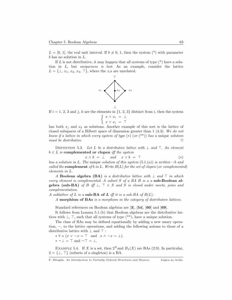
Chapter 5. Boolean Algebras 63
L = [0, 1], the real unit interval. If b 6= 0, 1, then the system (*) with parameterb has no solution in L.
If L is not distributive, it may happen that all systems of type (*) have a solu-tion in L, but uniqueness is lost. As an example, consider the latticeL = ⊥, x1, x2, x3, >, where the xis are unrelated.
>•
x1 x2• x3
• @@@
•
•⊥
@@@
If i = 1, 2, 3 and j, k are the elements in 1, 2, 3 distinct from i, then the systemx ∧ xi = ⊥x ∨ xi = >
has both xj and xk as solutions. Another example of this sort is the lattice ofclosed subspaces of a Hilbert space of dimension greater than 1 (4.3). We do notknow if a lattice in which every system of type (∗) (or (**)) has a unique solutionmust be distributive. 2
Definition 5.3. Let L be a distributive lattice with ⊥ and >. An elementb ∈ L is complemented or clopen iff the system
x ∧ b = ⊥ and x ∨ b = > (∗)has a solution in L. The unique solution of this system (5.1.(a)) is written ¬ b andcalled the complement of b in L. Write B(L) for the set of clopen (or complemented)elements in L.
A Boolean algebra (BA) is a distributive lattice with ⊥ and > in whichevery element is complemented. A subset S of a BA B is a a sub-Boolean al-gebra (sub-BA) of B iff ⊥, > ∈ S and S is closed under meets, joins andcomplementation.
A sublattice of L is a sub-BA of L iff it is a sub-BA of B(L).
A morphism of BAs is a morphism in the category of distributive lattices.
Standard references on Boolean algebras are [3], [54], [60] and [69].
It follows from Lemma 5.1.(b) that Boolean algebras are the distributive lat-tices with ⊥, >, such that all systems of type (**), have a unique solution.
The class of BAs may be defined equationally by adding a new unary opera-tion, ¬ , to the lattice operations, and adding the following axioms to those of adistributive lattice with ⊥ and > :
∗ ∀ x (x ∨ ¬x = > and x ∧ ¬x = ⊥).
∗ ¬⊥ = > and ¬> = ⊥.
Example 5.4. If X is a set, then 2Xand Bλ(X) are BAs (2.9). In particular,2 = ⊥, > (subsets of a singleton) is a BA.
F. Miraglia. An Introduction to Partially Ordered Structures and Sheaves. Logica no Aviao.
Chapter 5. Boolean Algebras 64
If T is a topological space, the lattice of clopens in T (3.6, 4.6), B(T ), is pre-cisely B(Ω(T )), and hence a BA. It will be shown latter that all Boolean algebrasare isomorphic to B(X), for some topological space X.
The lattice of regular opens in T , Reg(T ), is also a BA (1.14) although not asub-BA of Ω(T ). 2
Definition 5.5. If B is a Boolean algebra and a, b ∈ B, define the operationof implication by the rule
a → b = ¬ a ∨ b.We also define the operations of equivalence and symmetric difference by
a ↔ b = (a → b) ∧ (b → a) and a 4 b = (a ∧ ¬ b) ∨ (b ∧ ¬ a),
respectively.
Lemma 5.6. Let Lf−→ K be a morphism of distributive lattices and let
x, y ∈ L.
a) If x ∈ B(L), then fx ∈ B(K) and f(¬x) = ¬ f(x).
b) If L is a Boolean algebra, then,
i) f(¬x) = ¬ f(x); ii) f(x → y) = fx → fy;
iii) f(x ↔ y) = fx ↔ fy; iv) f(x 4 y) = fx 4 fy.
Moreover, f is a BA-morphism from L into B(K).
c) If L is a BA, f(L) is a sub-BA of K.
Proof. a) Since f preserves ∧ and ∨, as well as ⊥ and >, we havex ∧ ¬x = ⊥x ∨ ¬x = >
implies
fx ∧ f(¬x) = ⊥fx ∨ f(¬x) = >
which, in view of the distributivity of K and 5.1, shows that f(¬x) is ¬ f(x).Items (b) and (c) follow from (a) and the definitions of →, ↔ and 4.
Lemma 5.7. Let B be a BA and let x, y, z be elements in B. Then,
a) (The law of double negation) ¬¬x = x.
b) (x ∧ y) ≤ z iff x ≤ (¬ y ∨ z).
c) x ∧ y = ⊥ iff x ≤ ¬ y.
d) (The contrapositive law) x ≤ y iff ¬ y ≤ ¬x.
e) ¬ (x ∧ y) = ¬x ∨ ¬ y; ¬ (x ∨ y) = ¬x ∧ ¬ y.
f) For all S ⊆ B,
(1) If∨S exists in B, then both
∧s∈S ¬ s and
∨s∈S (x ∧ s) exist in B and
x ∧∨S =
∨s∈S (x ∧ s) and ¬
∨S =
∧s∈S ¬ s.
(2) If∧S exists in B, then both
∨s∈S ¬ s and
∧s∈S (x ∨ s) exist in B and
x ∨∧S =
∧s∈S (x ∨ s) and ¬
∧S =
∨s∈S ¬ s.
Proof. a) Follows immediately from the uniqueness of complements.
b) If x ∧ y ≤ z, then
x = x ∧ > = x ∧ (y ∨ ¬ y) = (x ∧ y) ∨ (x ∧ ¬ y) ≤ z ∨ (x ∧ ¬ y)
= (z ∨ x) ∧ (z ∨ ¬ y) ≤ z ∨ ¬ y.
F. Miraglia. An Introduction to Partially Ordered Structures and Sheaves. Logica no Aviao.

Chapter 5. Boolean Algebras 65
Conversely, if x ≤ z ∨ ¬ y, then
x ∧ y ≤ (z ∨ ¬ y) ∧ y = (z ∧ y) ∨ (¬ y ∧ y) = (z ∧ y) ∨ ⊥= z ∧ y ≤ z,
as desired. Item (c) is an immediate consequence of (b), with z = ⊥.
d) If x ≤ y, then
x ∧ ¬ y ≤ y ∧ ¬ y = ⊥,
and hence x ∧ ¬ y = ⊥. But then, (c) implies that ¬ y ≤ ¬x. The converse issimilar, using (a).
e) With distributivity, it is straightforward to check that the sated formulas aresolutions of the system of equations defining complements.
f) For the first equality in (1), let b ∈ B satisfy (x ∧ s) ≤ b, for all s ∈ S. By(b), we get s ≤ ¬x ∨ b. Thus,
∨S ≤ ¬x ∨ b; another application of (a) yields
x ∧∨S ≤ b. Hence,
∨s∈S (x ∧ s) exists in B and is equal to x ∧
∨S.
For the version of de Morgan’s law in (1), let b ∈ B be such that b ≤ ¬ s,for all s ∈ S. Then, ∀ s ∈ S, b ∧ s = ⊥ and so
∨s∈S (b ∧ s) = b ∧
∨S = ⊥.
Hence, b ≤ ¬ (∨S). It remains to show that ¬ (
∨S) ≤
∧s∈S ¬ s. The method
is the same as above and will be omitted. The proof of (2) is similar, and in fact,a consequence of (1), by complementation.
The basic properties of the operation 4 are described in
Lemma 5.8. Let B be a Boolean algebra. For x, y, z ∈ B,
a) 〈B,4,⊥〉 is an Abelian group of exponent 2 (i.e., x 4 x = ⊥), whose zero is⊥.
b) x 4 y = ⊥ iff x = y; x 4 y = > iff x = ¬ y.
c) x ∧ (y 4 z) = (x ∧ y) 4 (x ∧ z).d) 〈B,4,∧,⊥,>〉 is a commutative ring with identity >, with ∧ as product and4 as addition.
e) (x ∧ y) ∧ (x 4 y) = ⊥; x 4 y = x ∨ y iff x ∧ y = ⊥.
f) x ∨ y = x 4 y 4 (x ∧ y) = (x 4 y) ∨ (x ∧ y).
g) (y 4 z) ≤ x iff x ∨ y = x ∨ z.
Proof. Items (a) through (d) are left to the reader.
e) For the first equation, we compute as follows, recalling (b) and (c) :
(x ∧ y) ∧ (x 4 y) = (x ∧ y ∧ x) 4 (x ∧ y ∧ y)
= (x ∧ y) 4 (x ∧ y) = ⊥.
It x ∧ y = ⊥, then, by 5.7.(c), x ≤ ¬ y and y ≤ ¬x. Hence,
x 4 y = (x ∧ ¬ y) ∨ (y ∧ ¬x) = x ∨ y,
as claimed. Conversely, if x ∨ y = x 4 y, then x ≤ x 4 y. Thus, using (c), we get
x = x ∧ (x 4 y) = x 4 (x ∧ y),
and so the cancellation law in the group 〈B,4,⊥〉 yields x ∧ y = ⊥, as desired.
f) For a, b ∈ B, we have
a = a ∧ > = a ∧ (b ∨ ¬ b) = (a ∧ b) ∨ (a ∧ ¬ b).Hence,
F. Miraglia. An Introduction to Partially Ordered Structures and Sheaves. Logica no Aviao.
Chapter 5. Boolean Algebras 66
x ∨ y = [(x ∧ y) ∨ (x ∧ ¬ y)] ∨ [(y ∧ x) ∨ (y ∧ ¬x)]
= (x ∧ y) ∨ [(x ∧ ¬ y) ∨ (y ∧ ¬x)] = (x ∧ y) ∨ (x 4 y)
= (x ∧ y) 4 (x 4 y),
where the last equality comes from item (e).
g) First assume that (y 4 z) ≤ x. Then,
y 4 z = x ∧ (y 4 z) = (x ∧ y) 4 (x ∧ z), (I)
and so, since B is an Abelian group under 4, (I) is equivalent to
y 4 (x ∧ y) = z 4 (x ∧ z). (II)
Hence, item (f) and (II) yield
x ∨ y = x 4 y 4 (x ∧ y) = x 4 z 4 (x ∧ z) = x ∨ z.For the converse, assume that x ∨ y = x ∨ z. This equality can be written as
x 4 y 4 (x ∧ y) = x 4 z 4 (x ∧ z),which upon cancellation of x on both sides, leads us back to (II). But we knowthat (II) is equivalent to (I), ending the proof.
The fundamental properties of implication and equivalence are in
Lemma 5.9. Let B be a Boolean algebra. For x, y and z ∈ B, the followinghold :
a) x ≤ (y → z) iff x ∧ y ≤ z;
b) x → y = max a ∈ B : x ∧ a ≤ y.c) x ≤ y iff x → y = >; ¬x = (x → ⊥).
d) (modus ponens) x ∧ (x → y) ≤ y.
e) (contrapositive) (x → y) = (¬ y → ¬x).
f) x ≤ (y ↔ z) iff x ∧ y = x ∧ z.
Proof. (a) follows immediately from the definition of (y → z), while (b), (c)and (d) are simple applications of (a).
e) To show that (x → y) ≤ (¬ y → ¬x), it is enough to verify, by (a), that
¬ y ∧ (x → y) ≤ ¬x,
or equivalently, by Lemma 5.7.(c), that
x ∧ ¬ y ∧ (x → y) = ⊥.
But this follows immediately from the law of modus ponens (item (d)). Similarly,the reverse inequality is equivalent to
x ∧ (¬ y → ¬x) ≤ y. (I)
Since y = ¬¬ y (5.7.(a)), (5.7.(c)) implies that (I) is equivalent to
¬ y ∧ x ∧ (¬ y → ¬x) = ⊥,
which is, once again, a consequence of the law of modus ponens.
f) If x ≤ (y → z) = (y → z) ∧ (z → y), then (a) yields
x ∧ y ≤ z and x ∧ z ≤ y,
and so x ∧ y = x ∧ z. The converse is similar and left to the reader.
Our next result characterizes filters, ideals and the congruences they generatein terms of the operations of implication, equivalence and symmetric difference.
F. Miraglia. An Introduction to Partially Ordered Structures and Sheaves. Logica no Aviao.
Chapter 5. Boolean Algebras 67
Lemma 5.10. Let B be a Boolean algebra and x, y ∈ B.
a) A downward directed subset S of B is a filter iff
(F )
> ∈ S and
∀ x, y ∈ B, x, (x → y) ∈ S ⇒ y ∈ S.
b) An upward directed subset S of B is an ideal iff
(I)
⊥ ∈ S and
∀ x, y ∈ B, x, (x 4 y) ∈ S ⇒ y ∈ S.
c) With notation as in 4.9
(1) If F is a filter in B, then x ∼F y iff (x ↔ y) ∈ F .
(2) If I is an ideal in B, then x ∼I y iff (x 4 y) ∈ I.
Proof. a) Suppose that S satisfies (F ); if x ∈ S and x ≤ y, then, by 5.9.(c),(x → y) = > ∈ S, and so, y ∈ S. Moreover, if x, y ∈ S, since it is dd, thereis t ∈ S, such that t ≤ (x ∧ y). But then, we conclude from what has just beenproven, that (x ∧ y) ∈ S, and S is a filter (by 3.10.(a)).
Conversely, if S is a filter, it suffices to show that x ∈ S and (x → y) ∈ S,entails y ∈ S. But this follows immediately from the law of modus ponens (5.9.(d)).The proof of item (b) is analogous and we omit it.
c) We treat the case of ideals, leaving that of filters to the reader. For x, y ∈ B,we have suppose that x ∼I y. Then, there is t ∈ I, such that
x ∨ t = t ∨ y.
By Lemma 5.8.(g), (x4 y) ≤ t, and so (x4 y) ∈ I. Conversely, another applicationof 5.9.(g) yields
x ∨ (x 4 y) = y ∨ (x 4 y),
showing that (x 4 y) ∈ I implies x ∼I y.
A characterization of BAs among distributive lattices is given by
Proposition 5.11. Let L be a distributive lattice with ⊥ and >. Then, L isa BA iff for all θ ∈ Con(L), the congruence generated by Fθ is equal to θ.
Proof. By Exercise 5.18.(b), any congruence with respect to the latticeoperations in a BA is a congruence with respect to ¬.
Suppose L is a BA and θ ∈ Con(L). By Corollary 4.12, it is enough to provethat θ ⊆ ∼Fθ . To simplify notation, set
F = Fθ = x : x θ > and α = ∼Fθ .It must be shown that x θ y implies x ∼F y. Taking joins with ¬x on both sidesof (x θ y), yields (¬x ∨ x) θ (¬x ∨ y). Thus, (¬x ∨ y) is in F . Similarly, we have(¬ y ∨ x) ∈ F . F being a filter, we conclude
(x ↔ y) = (¬x ∨ y) ∧ (¬ y ∨ x) ∈ F .
It follows from Lemma 5.10.(c) that x ∼F y.
For the converse, we have to find a complement for each x ∈ L. Consider theideal I = x← and the congruence ∼I on B (4.10). By 5.18.(a), there is a filterF ⊆ B such that
F. Miraglia. An Introduction to Partially Ordered Structures and Sheaves. Logica no Aviao.
Chapter 5. Boolean Algebras 68
∀ a, b ∈ B, a ∼I b iff a ∼F b.
Since x ∼I ⊥, there is y ∈ F , with x ∧ y = ⊥. Because y ∈ F , we get y ∼F > andso y ∼I >; this means that there is t ≤ x, such that y ∨ t = > ∨ t = >. Clearly,y ∨ x = >, ending the proof.
In BAs, primeness and maximality for filters and ideals coincide.
Proposition 5.12. Let B be a Boolean algebra and let A be a proper filteror ideal in B. The following are equivalent :
(1) A is prime.
(2) For all x ∈ L, either x ∈ A or ¬x ∈ A.
(3) A is maximal.
Proof. Suppose that A is a filter in B. As usual, the case of ideals is dual.Since for all x ∈ B, x ∨ ¬x = > ∈ A, it is clear that (1) ⇒ (2). Now assume (2)and let G be a proper filter containing A. If x ∈ G, then ¬x cannot be in A, sincex ∧ ¬x = ⊥ and G is proper. Consequently, G ⊆ A and A is maximal. (3) ⇒ (1)follows from Lemma 4.22.(b).
Corollary 5.13. Let B be a Boolean algebra. There is a natural bijectivecorrespondence between the set of ultrafilters in B and the set of BA morphismsfrom B to 2 = ⊥, >, given by f 7→ cokerf .
Proof. Left to the reader.
Another characterization of Boolean algebras is given by
Proposition 5.14. A distributive lattice with ⊥ and > is a Boolean algebraiff every prime ideal is maximal.
Proof. We already know (5.12) that in a BA a filter is prime iff it is maximal.For the converse, suppose x ∈ L is not clopen. In particular x 6= ⊥, >. Set
A = z ∈ L : x ∧ z = ⊥.Then, A is an ideal and A ∪ x has the fup, otherwise x would have a complement.Let
F = y ∈ L : x ∨ y = > and I = i(A ∪ x) 1.
Clearly, F is a filter and I an ideal. To see that I ∩ F = ∅, consider what wouldhappen if there was t ∈ F ∩ I : in this case, x ∨ t = > and t ≤ x ∨ z, for somez ∈ A. But then
> ≤ (x ∨ t) ≤ x ∨ (x ∨ z) = x ∨ z,and z would be the complement of x. By Theorem 4.24, there is a prime filter Psuch that F ⊆ P and P ∩ I = ∅. In particular, x 6∈ P and P ∩ A = ∅. This lastequation means that P ∪ x has the fip; thus the proper filter it generates isstrictly larger than P , contradicting its maximality.
We invite the reader to supply a proof of the following preservation result.
1i(∗) is the ideal generated by ∗, as in 3.12.
F. Miraglia. An Introduction to Partially Ordered Structures and Sheaves. Logica no Aviao.
Chapter 5. Boolean Algebras 69
Proposition 5.15. The product, fiber product, and reduced product of Booleanalgebras are Boolean algebras.
The statement of the next result should be compared with 4.27.
Theorem 5.16. Let C ⊆ B be BAs. For every b ∈ B − C, there is anultrafilter F in C and ultrafilters F1, F2 in B, such that
(i) Fi ∩ C = F ; (ii) b ∈ F1 and ¬ b ∈ F2.
Proof. We freely employ the results in 5.7, without explicit mention.
Since b 6∈ C, the ideal I = b← ∩ C and the filter G = b→ ∩ C are disjoint inC. By Theorem 4.24 (and 5.12) , there is a ultrafilter F in C such that G ⊆ Fand F ∩ I = ∅.
We now verify that both F ∪ b and F ∪ ¬ b have the fip (3.13). If F ∪ bdid not have the fip, then for some a ∈ F , a ∧ b = ⊥. Hence, b ≤ ¬ a, and so¬ a ∈ G ⊆ F , which is impossible, because F is a proper filter. If F ∪ ¬ b didnot have the fip, then for some a ∈ F , we would have a ≤ b, untenable, becausethis implies a ∈ I and F is disjoint from this ideal, by construction.
By Theorem 4.25, there are ultrafilters F1, F2 in B, such that F ∪ b ⊆ F1
and F ∪ ¬ b ⊆ F2. Since F is maximal in C, it is clear that Fi ∩ C = F , endingthe proof.
The definitions of monic and epic appear in 16.8.
Proposition 5.17. Let Af−→ B be a BA morphism. Then,
a) f is monic iff it is injective iff coker f = >.
b) f is epic iff it is surjective.
Proof. a) is straightforward and left to the reader.
b) The argument here is more sophisticated, needing 5.16. All we have to do isverify that epic implies surjective (Exercise 16.38).
Suppose f is epic and there is b ∈ B − f(A). By 5.6.(c), f(A) is a sub-BA ofB. Let F , Fi, i = 1, 2 be the ultrafilters in f(A) and B constructed in 5.16. By5.13, B/Fi may be identified with 2 = ⊥, >. Let
B --
h1
h2
⊥, >
be the quotient maps induced by F1, F2, respectively. For a ∈ A,
h1(f(a)) = > iff f(a) ∈ F1 ∩ f(A) iff f(a) ∈ F2 ∩ f(A)
iff h2(f(a)) = >,
which shows that h1 f = h2 f . But this contradicts the hypothesis that f isepic, since h1(b) = >, while h2(b) = ⊥, that is, h1 6= h2.
F. Miraglia. An Introduction to Partially Ordered Structures and Sheaves. Logica no Aviao.

Chapter 5. Boolean Algebras 70
Exercises
5.18. Recall (2.32, 3.17) that if L is a lattice, F(L), I(L) are the poset offilters and ideals in L. Let B be a Boolean algebra.
a) Show that the map x 7→ ¬x induces an isomorphism from B onto Bop (which isalso a BA). Show that the above map induces a natural bijective correspondencebetween filters and ideals in B as follows
F ∈ F(B) 7→ ¬ F = b ∈ B : ¬ b ∈ F ∈ I(B).
Prove that this correspondence originates, in turn, a natural bijection between thecongruences generated by filters and ideals, in such a way that for all filters F inB, B/F is naturally isomorphic to B/¬ F .
b) Show that any lattice congruence on B is also a BA congruence, that is,preserves the operation ¬ . Conclude that any lattice congruence in a Booleanalgebra preserves implication, equivalence and symmetric difference.
c) If F is a filter in a BA B, then B/F is a BA and the canonical projection,
BπF−→ B/F , is a BA morphism. 2
5.19. Let B be a Boolean algebra. Show that the map
F ∈ F(B) 7−→ ∼F ∈ Con(B)
is an isomorphism between the lattice of filters in B (3.17.(d)) and the lattice ofcongruences in B. Conclude that the lattice of filters in a BA is a distributivelattice. State and prove a similar result for the lattice of ideals in a BA. 2
F. Miraglia. An Introduction to Partially Ordered Structures and Sheaves. Logica no Aviao.
CHAPTER 6
Heyting Algebras
The concept of Heyting algebra is an algebraic encoding of a constructivetheory of implication.
Definition 6.1. A Heyting algebra (HA) is a distributive lattice with ⊥and >, H, such that for all x, y ∈ H
max z ∈ H : z ∧ x ≤ y exists in H.
This element of H is denoted by x → y (x implies y). Hence, for all x, y, z ∈ H[→] x ∧ z ≤ y iff z ≤ (x → y).
If H and L are Heyting algebras, a map f : H −→ L is a HA-morphism ifff is a lattice morphism such that
∀ x, y ∈ H, f(x → y) = fx → fy.
Heyting algebras and their morphisms form a category, written HA.
Standard references on HAs are [3], [60] and [59].
Example 6.2. The algebra of opens of a topological space T provides one ofthe fundamental examples of Heyting algebras. The operation → is given by
U → V = int((T − U) ∪ V ).
In this Chapter it is recommended that the reader keep in mind the topologicalexample, together with the results in 1.14, that yield geometrical significance tomost of the constructions that follow.
A BA, B, is a Heyting algebra because for all x, y ∈ B, (¬x ∨ y) is the largestz ∈ B such that z ∧ x ≤ y (Lemma 5.7.(b)).
Chains or linear orders (with first and last element) are also HAs, where
x → y =
> if x ≤ y
y otherwise2
Remark 6.3. The class of HAs is equationally definable by adding a binaryoperation, →, to those of a lattice and adding, to the set of identities definingdistributive lattices with ⊥ and >, the following rules :
[HA 1] : x ∧ (x → y) = x ∧ y.
[HA 2] : x ∧ (y → z) = x ∧ ((x ∧ y) → (x ∧ z)).[HA 3] : z ∧ ((x ∧ y) → x) = z.
The reader is referred to Theorem IX.4.1, pg. 177, of [3]. In any case, this followseasily from the results to be presented below. 2
71
Chapter 6. Heyting Algebras 72
Some of the basic properties of Heyting algebras are presented in
Lemma 6.4. For x, y, z in a Heyting algebra H,
a) x ≤ y iff x → y = >.
b) (Modus Ponens) x ∧ (x → y) ≤ y.
c) x ≤ (x → y) → y and x ∧ (x → y) = x ∧ y.
d) y ≤ z implies
(x → y) ≤ (x → z)
and
(z → x) ≤ (y → x).
e) (y ∨ z) → x = (y → x) ∧ (z → x).
f) x → (y ∧ z) = (x → y) ∧ (x → z).
g) (x → t) ∨ (y → z) ≤ (x ∧ y) → (t ∨ z).
h) x → (y → z) = (x ∧ y) → z.
i) x ∧ (y → z) = x ∧ ((x ∧ y) → (x ∧ z)).
Proof. (a) is clear; (b) comes from the fact that (x → y) is the largest z inH such that z ∧ x ≤ y. From (b), the definition of → will immediately yield thefirst statement in (c), while, taking the meet with x on both sides of (b), will giveus the second.
d) Note that (x → y) ≤ (x → z) is true iff x ∧ (x → y) ≤ z. But this followsimmediately from (b) and y ≤ z. Similarly, we have
y ∧ (z → x) ≤ z ∧ (z → x) ≤ x,
which is equivalent to the second assertion in (d).
e) It follows directly from (d) that the left side of (e) is less than or equal to itsright hand side. For the other inequality, note that
(y ∨ z) ∧ (y → x) ∧ (z → x) =
= [y ∧ (y → x) ∧ (z → x)] ∨ [z ∧ (y → x) ∧ (z → x)]
≤ [x ∧ (z → x)] ∨ [x ∧ (y → x)] ≤ x ∨ x = x.
Items (f) and (g) are similar and left to the reader.
h) Applying the definition of → successively, we get
t ≤ [x → (y → z)] iff x ∧ t ≤ (y → z) iff y ∧ x ∧ t ≤ z
iff t ≤ [(x ∧ y) → z],
as needed. Item (i) is left to the reader.
The reader will surely notice the resemblance of the above with some of theusual laws of Logic.
Definition 6.5. Let H be a Heyting algebra. For each x ∈ H, write
¬x =def (x → ⊥),
called the pseudo-complement of x in H.
Remark 6.6. a) If Hf−→ K is a HA-morphism, then f preserves pseudo-
complement, that is, f(¬x) = ¬ fx, ∀ x ∈ H.
b) Note that for x in a HA H,
F. Miraglia. An Introduction to Partially Ordered Structures and Sheaves. Logica no Aviao.

Chapter 6. Heyting Algebras 73
¬x is the largest z in H such that z ∧ x = ⊥.
In particular, ¬⊥ = > and ¬> = ⊥. Observe also that if an element x of H has acomplement then it must be equal to ¬x. Hence, this notation is consistent withthat adopted for BAs. In fact,
H is a BA iff for all x ∈ H, x ∨ ¬x = >. (*)
i.e., ¬x is the complement of x (see Exercise 6.26.(a)). 2
Example 6.7. a) In the HA of opens of a topological space T we have
¬U = int(T − U).
It is therefore easy to give examples of HAs of this type, in which the only clopenelements are ⊥ and >.
b) In a chain, ¬x = ⊥ for all x 6= ⊥. 2
The basic rules governing pseudo-complementation are described in
Lemma 6.8. For all x, y, t, z in a HA H, we have
a) y ≤ z ⇒ ¬ z ≤ ¬ y.
b) x ≤ ¬¬x and x ≤ y ⇒ ¬¬x ≤ ¬¬ y.
c) t ∧ x = ⊥ iff t ∧ ¬¬x = ⊥.
d) ¬x = ¬¬¬x and x ≤ ¬ y ⇒ ¬¬x ≤ ¬ y.
e) ¬ (y ∨ z) = ¬ y ∧ ¬ z.
f) ¬ (x ∧ y) = ¬¬ (¬x ∨ ¬ y).
g) ¬¬ (x ∧ y) = ¬¬x ∧ ¬¬ y.
h) (¬x ∨ y) ≤ (x → y) ≤ ¬¬ (¬x ∨ y).
i) ¬ (x → y) = ¬¬x ∧ ¬ y.
j) ¬¬ (x → y) = ¬¬x → ¬¬ y.
k) ¬¬x ≤ ¬¬ [(x ∧ ¬ y) ∨ y].
l) ¬ (x ∨ ¬x) = ⊥; ¬¬ (x ∨ ¬x) = >.
Proof. Item (a) comes from the second statement in Lemma 6.4.(d), withx = ⊥. The first part of (b) is an instance of the first inequality in Lemma 6.4.(c),with y = ⊥, while the second comes from a double application of (a).
c) Clearly, (b) yields t ∧ ¬¬x = ⊥ ⇒ t ∧ x = ⊥. On the other hand,
t ∧ x = ⊥ ⇒ t ≤ ¬x ⇒ ¬¬x ≤ ¬ t ⇒ t ∧ ¬¬x = ⊥.
The assertions in (d) are direct consequences of (c). Item (e) comes directly fromLemma 6.4.(e), with x = ⊥.
f) Lemma 6.4.(g), with t = z = ⊥, yields ¬x ∨ ¬ y ≤ ¬ (x ∧ y); from item (d)above, we get ¬¬ (¬x ∨ ¬ y) ≤ ¬ (x ∧ y). On the other hand, (e) and a repeateduse of (d) yield that ¬ (x ∧ y) ∧ x ∧ y = ⊥ implies
¬ (x ∧ y) ∧ ¬¬x ∧ ¬¬ y = ¬ (x ∧ y) ∧ ¬ (¬x ∨ ¬ y) = ⊥,
showing that ¬ (x ∧ y) ≤ ¬ (¬x ∨ ¬ y), completing the proof of (f). Item (g)follows easily from (e) and (f).
h) Since x ∧ (¬x ∨ y) = x ∧ y, it follows that (¬x ∨ y) ≤ (x → y). For the otherinequality in (h), we again use (d) and (e) :
F. Miraglia. An Introduction to Partially Ordered Structures and Sheaves. Logica no Aviao.
Chapter 6. Heyting Algebras 74
x ∧ ¬ y ∧ (x → y) = ⊥ ⇒ ¬¬x ∧ ¬ y ∧ (x → y) = ⊥⇒ ¬ (¬x ∨ y) ∧ (x → y) = ⊥⇒ (x → y) ≤ ¬¬ (¬x ∨ y).
Item (i) is an immediate consequence of (a), (c) and (h).
j) By (g), (b) and Modus Ponens (6.4.(b)), we have
¬¬x ∧ ¬¬ (x → y) = ¬¬ (x ∧ (x → y)) ≤ ¬¬ y,
and the adjunction [→] in 6.1 yields ¬¬ (x → y) ≤ ¬¬x → ¬¬ y. For the reverseinequality, from item (i) and Modus Ponens comes
(¬¬x → ¬¬ y) ∧ ¬ (x → y) = (¬¬x → ¬¬ y) ∧ ¬¬x ∧ ¬ y≤ ¬¬ y ∧ ¬ y = ⊥,
and so, by (a), (¬¬x → ¬¬ y) ≤ ¬¬ (x → y), as needed. Items (k) and (l) are leftto the reader.
Definition 6.9. If H is a HA, define, for x, y ∈ H,
x ↔ y = (x → y) ∧ (y → x),
called the equivalence operation in H.
Lemma 6.10. For x, y, z in a HA H,
a) z ≤ (x ↔ y) iff x ∧ z = y ∧ z.
b) (x ↔ y) = max z ∈ H : z ∧ x = z ∧ y. 2
Proposition 6.11. If L is a distributive lattice, then F(L) and I(L) 1 areHeyting algebras.
Proof. Write F for F(L). We shall prove the result for F , leaving thecorresponding statement for I(L) to the reader. We start by
Fact. F is a distributive lattice.
Proof. It is sufficient to verify that for F,K,G ∈ F ,
F ∩ (G ∨ K) ⊆ (F ∩ G) ∨ (F ∩ K).
Recall that F ∨ G is the filter generated by F ∪ G, as well as that in F , ⊥ = >and > = L.
If x ∈ (G ∨ K), by Lemma 3.13.(a), there are A ⊆f G and B ⊆f K, such thatx ≥
∧A ∧
∧B. Thus,
x = (x ∨∧A) ∧ (x ∨
∧B) = [
∧a∈A (x ∨ a)] ∧ [
∧b∈B (x ∨ b)]. (I)
If x ∈ F , then (x ∨ a) ∈ (F ∩ G), ∀ a ∈ A. Similarly, if b ∈ B, then (x ∨ b) ∈(F ∩ K). Hence, (I) expresses x as a meet of elements in (F ∩ G) ∪ (F ∩ K), asneeded.
The same argument will prove something stronger, namely, that for all F ∈ Fand Gi : i ∈ I ⊆ F ,
F ∩ (∨Gi) =
∨(F ∩ Gi).
To finish the proof, observe that for F,G,K ∈ F ,
F ∩ K ⊆ G ⇒ For all k ∈ K and x ∈ F , (x ∨ k) ∈ G.
1The lattice of filters and ideals in L, as in 2.32 and 3.17.(d).
F. Miraglia. An Introduction to Partially Ordered Structures and Sheaves. Logica no Aviao.

Chapter 6. Heyting Algebras 75
The set of all z ∈ L that satisfy this property is easily seen to be a filter in L, thatis,
F → G = z ∈ L : ∀ x ∈ F , (x ∨ z) ∈ G,and F is indeed a HA.
Remark 6.12. Let L be a distributive lattice. With notation as in Proposition6.11, if F ∈ F , then
¬F = z ∈ L : ∀ x ∈ F , (x ∨ z) = >.In the case of I(L), we have, for I, J ∈ I(L)
I → J = z ∈ L : ∃ x ∈ I such that x ∧ z ∈ J;¬ I = z ∈ L : ∃x ∈ I such that (x ∧ z) = ⊥.
The lattice of congruences of any lattice is also a HA. We defer the proof of thisfact to a later chapter. 2
Example 6.13. a) If B is a BA and x, y ∈ B, then
(x ↔ y) = (¬x ∨ y) ∧ (¬ y ∨ x) = (x ∧ y) ∨ (¬x ∧ ¬ y).
Hence, (x ↔ y) = ¬ (x 4 y) = > 4 (x 4 y), where 4 is symmetric difference(5.5).
b) If T is a topological space and U, V ∈ Ω(T ), then
(U ↔ V ) = int((T − U) ∪ V ) ∩ int((T − V ) ∪ U)
= int [(U ∩ V ) ∪ ((T − U) ∩ (T − V ))].
Thus, ↔ in Ω(T ) is the interior of ↔ in 2T . 2
Example 6.14. a) If f : X −→ Y is a continuous map of topological spacesX,Y , in general, f∗ : Ω(Y ) −→ Ω(X) (4.6) will not be a HA-morphism. Thesame counterexample presented in 4.6 for the non-preservation of regular opens,shows that ¬ need not be preserved by f∗. This will, in fact, lead to a change inthe concept of morphism when we deal with frames 2. Nevertheless, the definitionof HA-morphism given above has enough importance to merit discussion. It isinteresting to find conditions on f such that f∗ is a HA-morphism. One such isthat f be open.
b) If C and L are chains, then f : C −→ L is a HA-morphism iff f is strictlyincreasing on C − coker f . 2
Proposition 6.15. Let H be a HA and F be a filter in H.
a) The equivalence relation ∼F generated by F is a congruence with respect to allthe operations on H. Furthermore, for x, y ∈ H
x ∼F y iff (x ↔ y) ∈ F .
b) The following are equivalent :
(1) F is an ultrafilter;
(2) F is prime and for all x ∈ H, ¬¬x ∈ F ⇒ x ∈ F ;
(3) For all x ∈ H, either x ∈ F or ¬x ∈ F .
c) If θ is a Heyting algebra congruence on H, then ∼Fθ = θ. The mapping
2Called complete Heyting algebras in [15] and complete pseudo-Boolean algebras in [60].
F. Miraglia. An Introduction to Partially Ordered Structures and Sheaves. Logica no Aviao.
Chapter 6. Heyting Algebras 76
F ∈ F(H) 7→ ∼F ∈ Con(H)
is an isomorphism from F(H) onto Con(H), the lattice of HA congruences onH.
d) If f is a HA-morphism, then f is injective iff coker f = >.
Proof. a) We first verify that
x ∼F y iff (x ↔ y) ∈ F .
If x ∼F y, then, there is z ∈ F such that x ∧ z = y ∧ z. By 6.10.(a), z ≤ (x↔ y),and so (x ↔ y) ∈ F . The converse is consequence of 6.10.(b), that is,
x ∧ (x ↔ y) = y ∧ (x ↔ y).
To complete the proof of (a), it is sufficient to show that
x ∼F y and a ∼F b ⇒ (x → y) ∼F (a → b).
Using the result just proven and Exercise 6.23.(b), we get
z = [(x ↔ y) ∧ (a ↔ b)] ∈ F and z ∧ (x → y) = z ∧ (a → b),
and so ∼F is a congruence with respect to →.
b) (1) ⇒ (2) : By 4.22, every ultrafilter is prime. If x 6∈ F , then the filter generated
by F and x cannot be proper. By 3.13.(a), there is a ∈ F such that a ∧ x = ⊥,that is, a ≤ ¬x. But then, ¬x ∈ F and F is not a proper filter. Hence, x ∈ F , asdesired.
(2) ⇒ (3) : By 6.8.(l), for all x ∈ H, ¬¬ (x ∨ ¬x) = > ∈ F ; therefore, (2) entails
(x ∨ ¬x) ∈ F and primeness yields the alternative in (3).
(3) ⇒ (2) : The proof is the same as that for BAs, in 5.12.
c) By 4.12.(c), it is enough to verify that θ ⊆ ∼Fθ . If x θ y, applying (x → ·) toboth sides of this relation yields > θ (x→ y). Similarly, we can show > θ (y → x).Hence, (x ↔ y) ∈ Fθ, which entails, by item (a), x ∼Fθ y. The remainder of (c),as well as (d), are left to the reader.
Corollary 6.16. If F is a filter in a HA H, the quotient H/F is a Heytingalgebra and the quotient morphism, πF : H −→ H/F is a HA-morphism.
Remark 6.17. a) Note that 6.15.(c) refers only, – as it must –, to HA-congruences. In 4.16 there is an example of a lattice congruence on the HA Ω(T )which does not come from a filter or ideal in Ω(T ). By 6.15.(c), that congruenceis not a HA-congruence on Ω(T ), something that can be checked directly.
Since Proposition 5.14 guarantees that a distributive lattice L is a BA iff alllattice congruences on L come from filters, and Ω(T ) is not a BA, such exampleswere certain to exist.
b) In general, the equivalence relation determined by ideals in a HA will notpreserve →, i.e., ∼I is not a HA-congruence. As an example, consider the idealI = (0,∞)←, generated by the open positive axis in the HA of opens of the realline, Ω(R). Clearly, (0, ∞) ∼I ⊥; but ¬ (0, ∞) = ( −∞, 0) is not equivalent to>, since there is no U ∈ I such that U ∪ (−∞, 0) = R. Hence, 6.16 is false forideals. 2
Example 6.18. Let H = [0, 1] be the real unit interval.
F. Miraglia. An Introduction to Partially Ordered Structures and Sheaves. Logica no Aviao.
Chapter 6. Heyting Algebras 77
a) DH = (0, 1], because for all x 6= 0 in H, ¬x = 0.
b) The filters on H are the principal filters and the intervals (x, 1], x 6= 0, allprime filters. But the only ultrafilter is DH = (0, 1]. This very simple examplealready displays an important fact : in Heyting algebras, prime filters have greatersignificance than ultrafilters. 2
The next theme is the discussion of a special type of filter in HAs, that willlead to a connection between Heyting and Boolean algebras. The analogy withtopological spaces is at the root of
Definition 6.19. Let H be a Heyting algebra and let x, y be elements of H.
a) x is dense in y iff x ≤ y ≤ ¬¬x. Write D(y) for the set of elements densein y.
b) x is dense iff ¬¬x = >. Write DH for the set of dense elements of H. WhenH is clear from context it will be omitted from the notation.
c) x is regular iff ¬¬x = x. Write Reg(H) is the set of regular elements in H.
Proposition 6.20. Let H be a HA and x, y ∈ H.
a) (x ∨ ¬x) ∈ D.
b) If y ∈ Reg(H), then
x → y = ¬¬x → y;
(x → y) ∈ Reg(H).
c) D is a proper filter in H and Reg(H) is closed under meets. Moreover, for allx, y ∈ H, x ∼D y iff ¬¬x = ¬¬ y.
d) A prime filter in H is maximal iff it contains D.
e) F and G are ultrafilters in H, then
F = G iff F ∩ Reg(H) = G ∩ Reg(H).
f) If Hf−→ P is a HA-morphism, then
f(DH) ⊆ DP and f(Reg(H)) ⊆ Reg(P ).
Proof. Item (a) is a consequence of 6.8.(l).
b) To prove the equality in the statement, it is enough, by 6.4.(d), to show that(x → y) ≤ (¬¬x → y). By the fundamental adjunction [→] in 6.1, this means
¬¬x ∧ (x → y) ≤ y. (I)
But we have, recalling 6.8.(j) and Modus Ponens
¬¬x ∧ (x → y) ≤ ¬¬x ∧ ¬¬ (x → y) = ¬¬x ∧ (¬¬x → ¬¬ y)
≤ ¬¬ y = y,
establishing (I), as needed. It now clear that if y ∈ Reg(H), then ¬¬ (x → y) =x → y, completing the proof of (b).
c) The first assertion in (c) is an immediate consequence of the fact that ⊥ 6∈ Dand 6.8.(g). For x, y ∈ H, by 6.15.(a) and 6.8.(g)
x ∼D y iff (x ↔ y) ∈ D iff ¬¬ (x ↔ y) = > = (¬¬x ↔ ¬¬ y)
iff ¬¬x = ¬¬ y,
as desired. Items (d) and (e) follow from 6.15.(b), while (f) is straightforward.
F. Miraglia. An Introduction to Partially Ordered Structures and Sheaves. Logica no Aviao.
Chapter 6. Heyting Algebras 78
Proposition 6.21. If H is a HA, then H/D is a BA, satisfying the followinguniversal property :
For all BAs B and all HA-morphisms Hf−→ B, there is a unique HA-
morphism, H/Dg−→ B, such that g πD = f .
B
H
?
- H/D
f
πD
g
Moreover, the map
u ∈ Reg(H) 7→ u/D ∈ H/Dis a BA-isomorphism of Reg(H) (6.24) onto H/D.
Proof. We already know that H/D is a HA. Note that for x ∈ Hx/D ∨ ¬x/D = (x ∨ ¬x)/D = >/D,
because ¬¬ (x ∨ ¬x) = > (6.20.(a) and (c)). It now follows from (*) in Remark6.6.(b) that H/D is a Boolean algebra. If f : H −→ B is a HA-morphism andx ∈ D, then
f(x) = ¬¬ f(x) = f(¬¬x) = f(>) = >,
and so D ⊆ coker f . By 4.13, there is a unique lattice morphism, g : L/D −→ B,making the displayed diagram commute. It now follows from 5.6.(b) that g is aBA-morphism. The remaining assertions are left to the reader.
The preceding results yield
Corollary 6.22. Let H be a HA. With notation as in 6.21, there are naturalbijective correspondences between
(1) The ultrafilters in H/D and the ultrafilters in H, given by F 7→ π−1D (F ).
(2) The HA-morphisms from H into 2 = ⊥, >, and the ultrafilters in H, givenby f 7→ cokerf .
Exercises
6.23. If ∗ is any of the binary operations in a HA H, then, for x, y, a, b ∈ H,
a) (a ∗ x) ∧ (x ↔ y) = (a ∗ y) ∧ (x ↔ y).
b) (a ∗ x) ∧ (x ↔ y) ∧ (a ↔ b) = (b ∗ y) ∧ (x ↔ y) ∧ (a ↔ b). 2
6.24. If H is a HA, define an operation ∨∗ on H by
a ∨∗ b = ¬¬ (¬¬ a ∨ ¬¬ b) = ¬¬ (a ∨ b).a) Reg(H) is closed under the operation ∨∗ and for a, b ∈ Reg(H),
F. Miraglia. An Introduction to Partially Ordered Structures and Sheaves. Logica no Aviao.
Chapter 6. Heyting Algebras 79
a ∨∗ b = sup a, b in the poset Reg(H).
b) Show that Reg(H) is a BA (the BA of regular elements in H.). 2
6.25. Let H be a HA and S be a subset of H. Show that
a) If∨S exists in H, then so does
∧s∈S ¬ s and ¬ (
∨S) =
∧s∈S ¬ s.
b) Investigate what happens in the case dual to (a). 2
6.26. Let H be a HA.
a) The following are equivalent :
(1) H is a BA.
(2) For all x ∈ H, x ∨ ¬x = >.
(3) For all x ∈ H, ¬¬x = x.
(4) The only dense element in H is >.
(5) Every prime filter in H is maximal.
(6) For all x, y ∈ H, (x → y) = ¬x ∨ y.
b) The following are equivalent :
(1) For all x, y ∈ H, ¬ (x ∧ y) = ¬x ∨ ¬ y.
(2) For all x ∈ H, ¬x ∨ ¬¬x = >. 2
F. Miraglia. An Introduction to Partially Ordered Structures and Sheaves. Logica no Aviao.
CHAPTER 7
Complete Lattices
One could view lattices as finitely complete posets. We now introduce theircomplete counterparts.
Definition 7.1. A partially ordered set L is complete (or a completelattice) if it satisfies the following equivalent conditions :
[∨
] : For all S ⊆ L,∨S exists in L;
[∧
] : For all S ⊆ L,∧S exists in L.
A subset S of a complete lattice L is a subbasis for L iff every element of Lis the join of finite meets of elements of S. S is a basis for L if every element ofL is the join of elements of S.
Note that all complete lattices have ⊥ and >. Among the examples in Chapter2, the reader will find many complete lattices. Of special importance here are thedistributive ones, particularly the algebra of opens of a topological space.
Remark 7.2. Let X be a set and S ⊆ 2X . In view of Lemma 1.8,
(i) S is a subbasis for τ(S), the topology generated by S on X.
(ii) S is a basis for a topology on X iff every element of B(S) is the union of ele-ments of S. In particular, this holds whenever S is closed under finite intersections,in which case B(S) = S. 2
Let A be a class of algebras, in which, among others, are defined the (possiblyinfinitary) partial operations ω1, . . . , ωn. If A, B ∈ A and f : A −→ B is a map,we say that
f is a [ω1, . . . , ωn]-morphism
iff f preserves all the operations ω1, . . . , ωn, that is, for all 1 ≤ j ≤ n, if ωj is definedin a = 〈 aα 〉α∈λ ∈ Aλ (λ a cardinal), then ωj is defined in f(a) = 〈 f(aα) 〉α∈λ and
f(ωj(a)) = ωj(f(a)).
Definition 7.3. Let L and P be posets. Let f : L −→ P be a morphism ofposets. Then,
a) f is a∨
-morphism iff for all S ⊆ L,∨S exists in L ⇒
∨f(S) exists in P and f(
∨S) =
∨f(S).
We may also write that f preserves joins.
b) f is a∧
-morphism iff for all S ⊆ L,∧S exists in L ⇒
∧f(S) exists in P and f(
∧S) =
∧f(S).
We may also write that f preserves meets.
80
Chapter 7. Complete Lattices 81
c) f is a [∧,∨
]-morphism iff f preserves finite meets and all joins.
d) f is a complete morphism iff f is a [∨,∧
]-morphism.
e) f is a regular embedding iff f is an injective [∨,∧
]-morphism.
A sublattice L ⊆ P is a regular sublattice if the canonical map from L toP is a regular embedding.
Note that all the notions of morphism introduced above are closed under com-position.
Remark 7.4. In the definition of maps preserving infinitary operations, it isnot assumed that the posets involved are complete. In particular, for a sublatticeto be a regular sublattice, it is necessary and sufficient that any joins or meetsexisting in the sublattice also exist and be the same in the larger one. As anexample, consider the rationals naturally embedded in R. This will be importantwhen we discuss completions. 2
One of the basic tools in constructing complete lattices is
Theorem 7.5. (Tarski) Let f : L −→ L be a poset morphism, with L acomplete lattice. Then, the set of fixed points of f ,
Fix(f) = x ∈ L : fx = x,with the po induced by L, is a complete lattice. In particular, Fix(f) 6= ∅. Moreover,
a) If f satisfies ∀ x ∈ L, fx ≥ x, then the meet of all S ⊆ Fix(f) are the sameas in L, that is, the natural injection of Fix(f) into L is a
∧-morphism.
b) If f satisfies ∀ x ∈ L, fx ≤ x, then the join of all S ⊆ Fix(f) are the same asin L, that is, the natural injection of Fix(f) into L is a
∨-morphism.
Proof. Let S ⊆ Fix(f); we show that∧S exists in Fix(f), in the partial
order induced by L. Consider
T = p ∈ L : ∀ s ∈ S (p ≤ s and p ≤ fp).It is straightforward to check that for p ∈ T , fp ∈ T . It is also clear that S ⊆ T .
Let q =∨T , this join taken in L. Note that
x ∈ Fix(f) and x ≤ s, for all s ∈ S ⇒ x ∈ T .
Therefore, to verify that q =∧S in Fix(f), it is enough to show that q ∈ Fix(f).
Since p ≤ s, for all 〈 p, s 〉 ∈ T × S, q is a lower bound for S. Furthermore, foreach p ∈ T , p ≤ q and so p ≤ fp ≤ fq. This means that fq is an upper bound forT and thus, q ≤ fq. We have shown that q ∈ T ; but then fq ∈ T and so fq ≤ q,proving that q ∈ Fix(f).
Now suppose fx ≥ x, ∀ x ∈ L. Let S ⊆ Fix(f) and t =∧S, this meet taken
in L. If t is proven to be a fixed point of f , then t will also be the meet of S inFix(f), as desired. Since f is increasing, we have ft ≤ fs = s, for all s ∈ S. Thus,ft is a lower bound for S in L. Consequently, ft ≤ t =
∧S, and so ft = t. The
case fx ≤ x is handled similarly. This ends the proof.
Example 7.6. In general, Fix(f) is not a sublattice of L. One simple reasonis that ⊥ and/or > might not be in their proper places. We now discuss slightlymore elaborate examples.
F. Miraglia. An Introduction to Partially Ordered Structures and Sheaves. Logica no Aviao.
Chapter 7. Complete Lattices 82
If T is a topological space we defined in section 1.2 two increasing maps of 2T
into itself, given by A 7→ int A and A 7→ A, whose basic properties are describedin 1.10. Notice that the fixed points of the first are the open sets in T , while thefixed points of the second are the closed sets in T ; in both cases, the lattice offixed points is a sublattice of 2T with arbitrary unions of opens being open andarbitrary intersections of closed sets being closed, illustrating the parts (b) and(c) of Theorem 7.5.
Now consider f , g : 2T −→ 2T given by
fA = intA and gA = int A.
Both maps are increasing, with Fix(f) corresponding to the regular closed setsi.e., closed sets F such that F = intF and Fix(g) corresponding to the lattice ofregular opens in T (3.6). If T = R, with its usual topology, then finite meets inFix(f) and finite joins in Fix(g) are not the same as in 2R. Simple examples maybe obtained by considering contiguous intervals, for instance [0, 1] and [1, 2] inFix(f) and (0, 1), (1, 2) in Fix(g). Although Fix(f) is a sub-∨-semilattice andFix(g) is a sub-semilattice of 2R, neither is a sublattice of 2R.
To construct an example such that neither finite meets nor finite joins arepreserved, it is sufficient to consider
f × g : 2R × 2R −→ 2R × 2R, given by (A,B) 7→ (fA, gB),
where the product lattice has its natural coordinatewise structure. Clearly, f × gis increasing and Fix(f × g) = Fix(f) × Fix(g). Thus, finite meets and joinsare not those induced by 2R × 2R. 2
Theorem 7.5 has many applications. Exercise 7.11 indicates two of these.
In complete lattices, a very general form of associativity holds for both meetsand joins, the proof of which is left to the reader :
Lemma 7.7. Let L be a complete lattice and Si, i ∈ I, be a family of subsetsof L. Then
a)∨i∈I (
∨Si) =
∨∨i∈I s(i) : s ∈
∏i∈I Si.
b)∧i∈I (
∧Si) =
∧∧i∈I s(i) : s ∈
∏i∈I Si. 2
With the infinitary versions of the distributive laws, the situation is quitedistinct. In Chapter 8, we discuss this situation in more detail (Proposition 8.7).
We now generalize what was done in Example 4.6.
Theorem 7.8. Let L and P be complete lattices. There is a natural bijective
correspondence between∨
-morphisms, Lf−→ P , and
∧-morphisms, P
g−→ L,defined by the rule :
[ad] ∀ u ∈ L and ∀ v ∈ P , fu ≤ v iff u ≤ gv.
In particular,
a) f g ≤ IdP and g f ≥ IdL.
b) g f g = g and f g f = f .
Proof. If g : P −→ L is a∧
-morphism, define f : L −→ P by
F. Miraglia. An Introduction to Partially Ordered Structures and Sheaves. Logica no Aviao.
Chapter 7. Complete Lattices 83
fu =∧v ∈ P : u ≤ gv.
It is immediate that f is increasing and that u ≤ gv ⇒ fu ≤ v. Assume nowthat fu ≤ v. Since g is increasing, g(fu) ≤ gv, while, the fact that g preserves
∧yields
g(fu) = g(∧v ∈ P : u ≤ gv) =
∧gv : u ≤ gv ≥ u.
Thus, u ≤ g(fu) ≤ gv and [ad] is verified.
To prove that f is a∨
-morphism, let S ⊆ L. Since f is increasing we have∨s∈S fs ≤ f(
∨S). To show equality, it is enough to verify that for v ∈ P , if
fs ≤ v, ∀ s ∈ S, then v ≥ f(∨S). This can be obtained from [ad] as follows :
∀ s ∈ S (fs ≤ v) ⇒ ∀s ∈ S (s ≤ gv) ⇒∨S ≤ gv,
and so f(∨S)≤ v, as desired. Given a
∨-morphism, f : L−→ P , define g : P −→ L
by dualizing what was done above :
gv =∨u ∈ L : fu ≤ v.
Analogous arguments will show that [ad] holds and that g is a∧
-morphism. It isstraightforward to show that the property [ad] uniquely determines the pair 〈 f, g 〉,as well as that it implies items (a) and (b) in the statement.
A pair (f , g) as in Theorem 7.8 will be called an adjoint pair with f the leftadjoint of g and g the right adjoint of f .
Corollary 7.9. Let f : L −→ P and g : P −→ L be an adjoint pair of mapsbetween complete lattices, with f a
∨-morphism and left adjoint to g.
a) The following conditions are equivalent :
(1) f is onto; (2) g is a section for f , that is, f g = IdP ;
(3) g is injective; (4) ∀ v ∈ P , g(v) = max f−1(v).
b) The following conditions are equivalent :
(1) f is injective; (2) f is a section for g, that is g f = IdL;
(3) g is onto; (4) ∀ u ∈ L, f(u) = min g−1(u).
Proof. We give a proof of the equivalence in (a), leaving the dual (b) as anexercise. Recall that the following adjointness condition is verified :
[ad] ∀ (u, v) ∈ L × P , fu ≤ v iff u ≤ gv,
as well as relations (a) and (b) in the statement of Theorem 7.8.
For (1) ⇒ (2), note that Theorem 7.8.(b) and the fact that f is onto yield, forv = fu,
f(g(v)) = f(g(f(u))) = fu = v,
as needed. (2) ⇒ (3) is clear. For (3) ⇒ (4), we have, for v ∈ P , g(f(g(v))) = gv(7.8.(b)); the injectivity of g implies f(g(v)) = v and so gv ∈ f−1(v). It followsdirectly from [ad] that gv is the largest element in f−1(v). (4) ⇒ (1) is immediateand the proof is ended.
Remark 7.10. Although in important cases (e.g., Example 6.2) the∨
-morphism f in Theorem 7.8 is a [∧,
∨]-morphism, g will not be a [∨,
∧]-morphism,
F. Miraglia. An Introduction to Partially Ordered Structures and Sheaves. Logica no Aviao.
Chapter 7. Complete Lattices 84
that is, g will not be a lattice morphism (it is always increasing or a poset mor-phism). As an example, consider the absolute value function av : R −→ R+. Withnotation as in Example 6.2 and using the formula given therein for av∗, it is easilychecked that
(i) av∗((0, ∞)) = av∗(( −∞, 0)) = ∅, while (ii) av∗(R − 0) = R+ − 0. 2
Most authors register the fact that Theorem 7.8 is a consequence of the AdjointFunctor Theorem (see Theorem 16.35).
In [17] adjoint pairs are called Galois connection; [17] contains interestingapplications of adjoint pairs, as well as references to the literature.
Exercises
7.11. Show that Theorem 7.5 implies the Cantor-Bernstein Theorem and thepossibility of defining functions by transfinite induction over well ordered sets. 2
7.12. This exercise consists in showing that the conditions in Theorem 7.8 areequivalent.
Let f : L −→ P and g : P −→ L be a∨
-morphism and a∧
-morphism ofcomplete lattices, respectively. The following are equivalent :
(1) 〈 f, g 〉 is an adjoint pair;
(2) f g ≤ IdP and g f ≥ IdL;
(3) g f g = g and f g f = f . 2
F. Miraglia. An Introduction to Partially Ordered Structures and Sheaves. Logica no Aviao.
CHAPTER 8
Frames
We now introduce the algebraic constructs that are fundamental in all thatfollows.
Definition 8.1. A complete lattice, L, is a frame if it satisfies the followingdistributive law :
[∧,∨
] For all S ⊆ L and all x ∈ L, x ∧∨S =
∨s∈S x ∧ s.
It is clear that any frame is a distributive lattice.
If L and L′ are frames, a map f : L −→ L′ is a frame morphism iff it isa [∧,
∨]-morphism of complete lattices, i.e., f preserves finite meets and arbitrary
joins.
If L is a frame, a subset K of L is a subframe of L if, when endowed withthe lattice structure induced by L, the canonical map from K to L is a framemorphism.
Write Frame for the category of frames and their morphisms.
Example 8.2. If X is a set, 2X with the usual set-theoretic operations is aframe. Moreover, the subframes of 2X are exactly the topologies on X. Althoughtopologies are fundamental examples of frames, other important instances of thisnotion will appear below. 2
Example 8.3. If (P , ≤) is a poset, let U(P ) be the topology on P generatedby the set x→ : x ∈ P (1.8). Note that :
i) Each x ∈ P has a smallest open neighborhood, namely x→.
ii) Opens of the form x→ are super compact, that is, any open covering has anone element sub covering.
iii) The frame of opens of this topology on P is an algebraic frame, since everyopen U can be written as U =
⋃x∈U x→.
In [15], the frame of opens of this topology on P are called Kripke models. 2
Induction and the [∧,∨
] law yields
Corollary 8.4. Let H be a frame and S1, . . . , Sn be subsets of H. Then∧ni=1 (
∨Si) =
∨∧ni=1 t(i) : T ∈
∏Si. 2
Lemma 8.5. A frame L has a natural structure of Heyting algebra, with im-plication given, for p, q ∈ L, by
p → q =∨x ∈ L : x ∧ p ≤ q,
and satisfying the fundamental adjunction [→] in Definition 6.1.
85
Chapter 8. Frames 86
Proof.1 Fix p, q ∈ L and set
t =∨x ∈ L : x ∧ p ≤ q. (1)
If S is the subset of L in the right-hand side of (1), the fact that L satisfies the[∧,∨
]-law yields
p ∧ t = p ∧∨S =
∨x∈S p ∧ x ≤ q,
showing that, in fact, t = max x ∈ L : p ∧ x ≤ q, as needed.
If L is a frame, the operation of implication in L will always be thecanonical operation associated to L as in Lemma 8.5.
It was shown in Lemma 7.7, that a very general form of associativity holds inany complete lattice. On the other hand, infinitary versions of distributivity yieldcharacterizations of some the algebraic objects we have been describing. We startwith
Definition 8.6. Let L be a lattice.
a) L is a [∧,∨
]-lattice iff it satisfies
[∧,∨
]For all S ⊆ L and all x ∈ L, if
∨S exists in L, then∨
s∈S (x ∧ s) exists in L and x ∧∨S =
∨s∈S (x ∧ s).
b) L is a [∨,∧
]-lattice iff it satisfies
[∨,∧
]For all S ⊆ L and all x ∈ L, if
∧S exists in L, then∧
s∈S (x ∨ s) exists in L and x ∨∧S =
∧s∈S (x ∨ s).
Proposition 8.7. a) Chains and BAs are [∨,∧
]−lattices.
b) Every HA is a [∧,∨
]-lattice. In particular, every BA and all chains are [∧,∨
]-lattices.
c) A HA is a frame iff it is complete as a lattice. In particular, complete chainsare frames.
Proof. a) The statement for BAs follows from 5.7.(g). For chains, the veri-fication is straightforward.
b) Let L be a HA, S ⊆ L and suppose that∨
S exists in L. Assume that fort, x ∈ L, we have t ≥ x ∧ s, ∀ s ∈ S. Then, s ≤ x → t, for all s ∈ S and so∨
S ≤ x → t. But this means that x ∧∨S ≤ t. This reasoning proves, in one
stroke, that∧s∈S (x ∧ s) exists in L and is equal to x ∧
∨S. Item (c) follows
immediately from (b) and Definition 8.1, ending the proof.
Remark 8.8. Important references in the subject, [15] among them, use theterm complete Heyting algebras (cHa) for what we here are designating as frames.Proposition 8.7 surely describes grounds on which this nomenclature is reasonable.It should be nevertheless registered that a frame and a Heyting algebra, that iscomplete as a lattice, are algebras of different types, although in a certain senseinterpretable in one another.
In [60], frames and cHas are called complete pseudo Boolean algebras . 2
1See also Exercise 8.27.
F. Miraglia. An Introduction to Partially Ordered Structures and Sheaves. Logica no Aviao.

Chapter 8. Frames 87
Definition 8.9. A complete Boolean algebra (cBa) is a BA that is com-plete as a lattice. The category cBa of complete Boolean algebras is the categorywhose objects are cBas and whose morphisms are [∧,
∨]-morphisms. By Proposi-
tion 8.7.(b) cBa is a subcategory of Frame.
Example 8.10. It is clear that 2X is a complete Boolean algebra. By Lemma1.14 and Example 5.4, if T is a topological space, Reg(T ) is a complete Booleanalgebra. 2
Definition 8.11. A frame morphism, f : L −→ R, is
a) implication preserving (ip) if
For all p, q ∈ L, f(p → q) = fp → fq.
b) open if it is an implication preserving, [∨,∧
]-morphism, of complete lattices.
Remark 8.12. Our definition of frame morphism has its origin in Topology(Examples 4.6 and 6.14). Analogy with Topology is also the source of the term“open” for a complete morphism which preserves implication : if f : X −→ Y is acontinuous open map of topological spaces, then f∗ : Ω(Y ) −→ Ω(X) is a completemorphism such that, for all U, V ∈ Ω(Y ), f∗(U → V ) = f∗U → f∗V .
In [15], open is used for what we here call a complete morphism. Hence, theexamples below may be instructive :
1. A regular embedding that does not preserve implication. Let [0, 1] be the closedreal unit interval and L = Ω((0, 1)) be the frame of opens of the open unit interval(0, 1). Define f : [0, 1] −→ L by r 7→ (0, r) (with f(0) = ∅); clearly, f is a completeembedding. On the other hand, for all r < s in (0, 1),
s → r = r in [0, 1], while (0, s) → (0, r) = (0, r) ∪ (s, 1) in L.
2. An implication preserving frame morphism that is not open. If L is a frame, let
D = ¬¬x ∈ L : x ∈ L,be the filter of dense opens in L, where as usual ¬x =def x → ⊥. Corollary 10.5and Example 8.18, the canonical quotient map from L to L/D is an implicationpreserving frame morphism, that, in general, does not preserve arbitrary meets.
In view of (1) and (2), it seemed reasonable to reserve the term open for thosemorphisms that had properties more closely resembling the topological case.
Example (1) also shows that a subobject in the category Frame may not bea Heyting subalgebra. 2
Other examples of frames are described in
Corollary 8.13. If L is a lattice, then Con(L) is a frame.
Proof. If θ and γi are in Con(L), it is sufficient to show that
θ ∧ (∨γi) ⊆
∨(θ ∧ γi).
By 4.18, this reduces to showing that for A ⊆f γi 2, θ distributes over the joinof the elements in A. But this comes immediately from 4.19, that guarantees thedistributivity of Con(L).
2⊆f means “finite subset of”.
F. Miraglia. An Introduction to Partially Ordered Structures and Sheaves. Logica no Aviao.

Chapter 8. Frames 88
There is method in this madness.
Proposition 8.14. A distributive algebraic lattice satisfies [∧,∨
]. In partic-ular, any complete distributive algebraic lattice is a frame.
Proof. Let L be a distributive algebraic lattice and S ⊆ L be such that∨S
exists in L. We will prove that for all x ∈ L,∨x ∧ s : s ∈ S = x ∧
∨S.
Fix a set C of compact elements in L such that x ∧∨
S =∨
C. Let p ∈ L besuch that p ≥ x ∧ s, for all s ∈ S. For each c ∈ C, c ≤ x and c ≤
∨S and so,
there is a finite subset s1, . . . , sn ⊆ S such that
c ≤ x ∧ (∨ni=1 si) =
∨ni=1 x ∧ si.
From p ≥ x ∧ s, s ∈ S, we get p ≥ c. Since this holds for all c ∈ C, we concludethat p ≥ x ∧
∨S, ending the proof.
In spite of the observation at the end of Remark 8.12, the following simpleresult will prove useful.
Corollary 8.15. Let H be a HA, P be a frame and Hf−→ P be an injective
lattice morphism such that f(H) is a basis for P . Then, f is a HA-morphism, thatis, for all x, y ∈ H, f(x → y) = fx → fy.
Proof. Since f is increasing and preserves meets, Modus Ponens yields
fx ∧ f(x → y) = f(x ∧ (x ∧ y)) ≤ f(y),
and so the adjunction [→] in 6.1 entails f(x → y) ≤ fx → fy. To prove equalityit is enough to check, again by [→], that
For all t ∈ P , t ∧ fx ≤ fy ⇒ t ≤ f(x → y).
Since f(H) is a basis for P , we may write t =∨z∈A fz, with A ⊆ H. Therefore,
the [∧,∨
]-law in P yields
t ∧ fx = fx ∧∨z∈A fz =
∨z∈A fx ∧ fz =
∨z∈A f(x ∧ z) ≤ fy.
Hence, for z ∈ A, we have f(x ∧ z) ≤ fy, or equivalently,
f(x ∧ z ∧ y) = f(x ∧ z);since f is injective, this implies x ∧ z ≤ y and so z ≤ x → y. But then,
For all z ∈ A, f(z) ≤ f(x → y),
that entails t =∨z∈A fz ≤ f(x → y), as desired.
The behavior of implication and pseudocomplementation with respect to theinfinitary operations in a frame is described in
Lemma 8.16. Let H be a frame and S ∪ x ⊆ H.
a)∧s∈S (x → s) = x →
∧S.
b)∧s∈S (s → x) =
∨S → x.
c)∨s∈S (x → s) ≤ x →
∨S.
d)∨s∈S (s → x) ≤
∧S → x.
e) ¬ (∨S) =
∧s∈S ¬ s.
f) ¬ (∧S) ≥ ¬¬ (
∨s∈S ¬ s) = ¬
∧s∈S ¬¬ s.
F. Miraglia. An Introduction to Partially Ordered Structures and Sheaves. Logica no Aviao.
Chapter 8. Frames 89
g) ¬¬∧s∈S ¬¬ s =
∧s∈S ¬¬ s.
h) ¬¬ (∨S) = ¬ (
∧s∈S ¬ s) = ¬¬ (
∨s∈S ¬¬ s).
In particular, in a cBa we have the de Morgan laws
¬∨
S =∧s∈S ¬ s and ¬
∧S =
∨s∈S ¬ s.
Proof. Part (a) is Exercise 8.28.(c). We prove (b), leaving (c) and (d) tothe reader. For each s ∈ S,
s ∧ (∧s∈S (s → x)) ≤ s ∧ (s → x) ≤ x,
and so (∨
S) ∧∧s∈S (s → x) ≤ x. Thus,
∧s∈S (s → x) ≤
∨S → x. By 6.4.(d),
(∨
S → x) ≤ (s → x). Thus,∨
S → x ≤∧s∈S (s → x), verifying (b).
e) We have
(∧s∈S ¬ s) ∧
∨S =
∨t ∧
∧s∈S ¬ s : t ∈ S = ⊥.
Thus, (∧s∈S ¬ s) ≤ ¬ (
∨S). To show equality, assume that
x ∧∨
S =∨x ∧ s : s ∈ S = ⊥.
Clearly, we must have, x ∧ s = ⊥, that is, x ≤ ¬ s, for all s ∈ S. From this, (e)follows immediately.
f) The equality in (f) follows from (e). For the inequality, note that
(∧
S) ∧∨s∈S ¬ s =
∨(¬ t) ∧
∧s∈S ¬¬ s) : t ∈ S = ⊥.
This yields∨s∈S ¬ s ≤ ¬
∧S. Therefore, taking the contrapositive (6.8.(a)) twice
(or using 6.8.(c)), yields the required result. The remaining items follow straight-forwardly from what has been proven.
Remark 8.17. It was shown in Lemma 5.7 that the general forms of thede Morgan laws held in a BA, whenever the appropriate joins and meets existed.Hence, if H is a frame and B a cBa,
every [∧,∨
]-morphism from B to H is an open morphism.
In particular, in the category cBa all morphisms are open. 2
Example 8.18. For finite subsets S of a HA we have
a) ¬∧
S = ¬¬∨s∈ S ¬ s (Lemma 6.8.(e));
b) ¬¬∧
S =∧s∈S ¬¬ s (Lemma 6.8.(f)).
However, these formulae do not hold for infinite subsets of a frame. As an example,consider, in Ω(R), the family S = R - p : p ∈ R. Then, for all U ∈ S, ¬¬U = Rand
∧S = ∅. Thus, ¬
∧S = >, while ¬¬
∨U∈S ¬U = ∅. Similarly, ¬¬
∧S =
∅, while ¬¬∧U∈S ¬¬U = R. Note that S ⊆ D, where D is the filter of dense
elements in Ω(R).
The reader is invited to prove that if H is a frame and S ⊆ H, then (a) isequivalent to (b).
A modification of the above example shows that Ω(R) does not satisfy[∨,∧
] :let S be as before and V 6= R be an open set, containing the rationals Q. Then,V ∨
∧S is distinct from
∧U∈S V ∨ U .
In [3] there is a characterization, due to Chang and Horn, of the lattices thatsatisfy [∧,
∨] and [∨,
∧] (Thm. XII.1.7, pg. 230). We have already remarked that
BAs and chains satisfy both generalized distributive laws (Proposition 8.7). 2
F. Miraglia. An Introduction to Partially Ordered Structures and Sheaves. Logica no Aviao.
Chapter 8. Frames 90
Although Example 8.18 shows that the [∨,∧
] distributive law does not hold ina frame L, there is a subset of L for which it holds true : the BA, B(L), of clopensin L (Definition 5.3). An important class of distributive lattices is described in
Definition 8.19. A complete distributive lattice L is zero-dimensionaliff B(L) is a basis for L.
In Chapter 18 of Part II, we present a whole class of frames, the algebraof opens of totally disconnected spaces, that are significant examples of zero-dimensional frames.
The clopens in a distributive lattice have a number of useful properties, someof which are described in
Lemma 8.20. Let L be a complete distributive lattice and b an element ofB(L).
a) The laws [∨,∧
] and [∧,∨
] hold for b and all S ⊆ L, that is
b ∨ (∧S) =
∧s∈S (b ∨ s) and b ∧
∨S =
∨s∈S (b ∧ s).
b) If L is a zero-dimensional frame, any element satisfying the [∨,∧
] law for allS ⊆ L is clopen.
c) If c is compact in L then b ∧ c is compact in L.
Proof. a) For the first equality, it is enough to show that∧s∈S (b ∨ s) ≤ b ∨
∧S.
Suppose t ≤ (b ∨ s), s ∈ S; then,
(t ∧ ¬ b) ≤ ¬ b ∧ (b ∨ s) = ¬ b ∧ s,and so (t ∧ ¬ b) ≤ ¬ b ∧
∧S. From b ∨ ¬ b = >, we get
t = (t ∧ b) ∨ (t ∧ ¬ b) ≤ (t ∧ b) ∨ (¬ b ∧∧S) ≤ b ∨
∧S,
giving the desired inequality. The proof of the second equation in the statement issimilar.
b) If L is zero-dimensional, let b ∈ L satisfy [∨,∧
] law, for all S ⊆ L. Since B(L)is a basis for L, we have b =
∨p∈A p, with A ⊆ B(L). For each p ∈ A, p ≤ b entails
b ∨ ¬ p = >. Thus,
> =∧p∈A (b ∨ ¬ p) = b ∨
∧p∈ A ¬ p.
Since L is a frame, we also have
b ∧∧q∈A ¬ q =
∨p∈A (p ∧
∧¬ q) = ⊥,
showing that b is complemented in L.
c) Let S ⊆ L be such that∨S ≥ b ∧ c. Then
¬ b ∨∨
S ≥ (c ∧ ¬ b) ∨ (c ∧ b) = c.
By compactness, ¬ b ∨∨
K ≥ c, with K ⊆f S. It is clear that∨K ≥ c ∧ b, and
b ∧ c is compact in L.
Definition 8.21. An element of a (not necessarily distributive) lattice L islinear if it satisfies the [∨,
∧]-law for all S ⊆ L.
Remark 8.22. It is clear that the set of linear elements in any lattice is closedunder finite sups.
F. Miraglia. An Introduction to Partially Ordered Structures and Sheaves. Logica no Aviao.

Chapter 8. Frames 91
By Lemma 8.20.(a), in distributive lattices, clopens are linear. However, theclopens are, in general, only a proper subset of the linear elements. For instance,in chains all elements are linear, but the only clopens are ⊥ and >. 2
We have already met a setting in which a complete lattice has to be a frame(Proposition 8.14). Another such situation is described in
Proposition 8.23. A complete zero-dimensional lattice is a frame iff it isdistributive.
Proof. Let L be a complete zero-dimensional distributive lattice and letS ∪ x ⊆ L. It is enough to verify that x ∧
∨S ≤
∨s∈S (x ∧ s). Let p ∈ B(L)
satisfy p ≤ x ∧∨S; then, p ∨ ¬ p = > yields
¬ p ∨ (x ∧∨S) = (¬ p ∨ x) ∧
∨s∈S (¬ p ∨ s) = >,
wherefore, ¬ p ∨ x = > and∨s∈S (¬ p ∨ s) = >. Hence, since ¬ p is linear (Lemma
8.20(a)),
¬ p ∨∨s∈S (x ∧ s) =
∨s∈S ¬ p ∨ (x ∧ s)
=∨s∈S (¬ p ∨ x) ∧ (¬ p ∨ s) = >,
and so p ≤∨s∈S (x ∧ s). Since L is zero-dimensional and p is an arbitrary clopen
below x ∧∨S, we obtain the inequality establishing that L is a frame.
An analysis of the proof of Proposition 8.23 leads to a very interesting result,due to Isbell ([31]; also [70]), giving a criterion for a complete lattice to be azero-dimensional frame, which circumvents first verifying that it is distributive.This will later be applied to show that the lattice of congruences in a frame iszero-dimensional. We follow, with minor modifications, the exposition of Isbell’sresult in [15].
We introduce a notion dual to that of basis. Let L be a complete lattice. Asubset S of L is a cobasis for L iff for all x, y ∈ L,
x ≤ y iff ∀s ∈ S (x ∨ s = > ⇒ y ∨ s = >).
With these preliminaries we are ready to prove
Theorem 8.24. (Isbell) A complete lattice is a zero-dimensional frame iff theset linear elements is a cobasis.
Proof. If L is a zero-dimensional frame, Lemma 8.20.(b) tells us that theset of linear elements is precisely B(L). Since L is distributive, for p ∈ B(L) andx ∈ L, we have p ≤ x iff ¬ p ∨ x = >. Thus, for all x, y ∈ L,
x ≤ y iff ∀ p ∈ B(L) (p ≤ x ⇒ p ≤ y)
iff ∀ q ∈ B(L) (q ∨ x = > ⇒ q ∨ y = >)
and so the set of linear elements is a cobasis for L. For the converse, we first verifythat L is a frame. For x ∪ S ⊆ L, we must prove that x ∧
∨S ≤
∨s∈S (x ∧ s).
Suppose that z is a linear element in L, such that z ∨ (x ∧∨S) = >. Once it is
proven that
z ∨∨s∈S (x ∧ s) = >,
F. Miraglia. An Introduction to Partially Ordered Structures and Sheaves. Logica no Aviao.

Chapter 8. Frames 92
the fact that the linear elements form a cobasis will give us the desired inequality.From z ∨ (x ∧
∨S) = > and the linearity of z comes
(*) z ∨ x = > = z ∨∨
S =∨s∈S (z ∨ s).
Thus, Lemma 7.7, the linearity of z and (*) yield
z ∨∨s∈S (x ∧ s) =
∨s∈S z ∨ (x ∧ s) =
∨s∈S (z ∨ x) ∧ (z ∨ s)
=∨s∈S z ∨ s = >,
showing that L is a frame. It remains to verify that the clopens in L are a basisfor L. A path is suggested by 8.20.(b) : prove that linear elements are clopen andso B(L) will be the set of linear elements. For, suppose that this is the case. If tis linear and x ∨ t = >, then ¬ t ≤ x and so
t ∨∨z ∈ B(L) : z ≤ x ≥ t ∨ ¬ t = >;
the linears being a cobasis, we obtain x ≤∨z ∈ B(L) : z ≤ x and B(L) is a
basis for L.
For a linear element t ∈ L, let z =∧y ∈ L : t ∨ y = >. By linearity, one
has t ∨ z = >. To prove that t ∈ B(L), it is sufficient to show that t ∧ z = ⊥. Letq be linear, such that q ∨ (t ∧ z) = >, that is, q ∨ t = > and q ∨ z = >. Sinceq ∨ t = >, we get z ≤ q. But then, q = z ∨ q = >. The above argument showsthat for all linear q in L, if q ∨ (t ∧ z) = >, then q = q ∨ ⊥ = >. The cobasisproperty then yields t ∧ z = ⊥, as needed.
We end this Chapter with the frame version of “disjointing an union of sets”.
Proposition 8.25. Let pi : i ∈ i be a family of elements in a frame H.Then, there is qi : i ∈ I ⊆ H, such that
(1) For all i ∈ I, qi ≤ pi;
(2) For all i 6= j in I, qi ∧ qj = ⊥;
(3)∨i∈I qi is dense in
∨i∈I pi (6.19.(a)).
Proof. We assume that I is well-ordered, with first element i0. By transfiniterecursion, define
∗ qi0 = pi0 ;
∗ Having defined qi, for i < j, set qj = pj ∧ ¬∨i<j pi.
It is clear that condition (1) is satisfied. If i 6= j, we may assume that i < j. Butthen, since qi ≤ pi ≤
∨k<j pk, we obtain
qi ∧ qj = qi ∧ pj ∧ ¬∨k<j pk = ⊥,
verifying (2). To establish (3) it is enough to show that for all j ∈ J ,
(*) pj ≤ ¬¬∨i≤j qi,
which shall be done by transfinite induction; clearly, (*) holds for the first elementi0 of I. Assume that (*) holds for all i < j. Note that the induction hypothesisentails
(**) ¬∨i<j qi = ¬
∨i<j pi.
Hence, (**), (e) and (k) in 6.8, together with 8.16.(e), yield
F. Miraglia. An Introduction to Partially Ordered Structures and Sheaves. Logica no Aviao.
Chapter 8. Frames 93
¬¬∨i≤j qi = ¬¬
(qj ∨
∨i<j qi
)= ¬
(¬ qj ∧ ¬
∨i<j qi
)= ¬
(¬ qj ∧ ¬
∨i<j pi
)= ¬¬
(qj ∨
∨i<j pi
)= ¬¬
((pj ∧ ¬
∨i<j pi) ∨
∨i<j pi
)≥ ¬¬ pj ,
ending the proof.
The law of double negation in Boolean algebras (5.7.(a)) yields
Corollary 8.26. Let pi : i ∈ i be a family of elements in a cBa B. Then,there is qi : i ∈ I ⊆ B, such that
(1) For all i ∈ I, qi ≤ pi;
(2) For all i 6= j in I, qi ∧ qj = ⊥;
(3)∨i∈I qi =
∨i∈I pi.
Exercises
8.27. Use Theorem 7.8 to construct implication in a frame and to immediatelyconclude item (a) in Lemma 8.16. 2
8.28. a) Show that the class of frames is closed under products and imagesby frame morphisms.
b) Examine what happens in 7.8 if we assume that L and P are cBas.
c) Let L be a complete lattice and d : L −→ L × L be the diagonal map,dx = 〈x, x 〉. Compute the right and left adjoints of d. 2
8.29. A distributive lattice is compact if >is compact (compare 2.43.(e)).Prove that a complete lattice is a compact zero-dimensional frame iff it is isomor-phic to the lattice of ideals of a BA. 2
F. Miraglia. An Introduction to Partially Ordered Structures and Sheaves. Logica no Aviao.

CHAPTER 9
Radical Ideals and Multiplicative Subsets
In general, the lattice of ideals of a commutative ring with identity, R, is notdistributive. The first section of this chapter is devoted to the construction of alattice of ideals in R that is distributive and, in fact, an algebraic frame : the latticeof radical ideals. When R is a Gaussian domain or Noetherian, there is anotheralgebraic frame associated to R, that of its saturated multiplicative subsets,discussed in section 2. The last section presents the ring of fractions generatedby a multiplicative subset of R. Most facts we shall use concerning commutativerings, if proofs are not provided, can be found in any standard text in CommutativeAlgebra, e.g., [2].
In what follows, all rings are commutative with identity 1.
1. Radical Ideals
Definition 9.1. Let R be a ring and S ⊆ R.
a) S is an ideal in R if for all x, y ∈ R∗ x, y ∈ S ⇒ x + y ∈ S; ∗ x ∈ R ⇒ xy ∈ S.
An ideal is proper if it is distinct from R.
b) The ideal generated by S is
(S) = t ∈ R :∃ s1, . . . , sn ∈ S and λ1, . . . , λn ∈ R
such that t =∑ni=1 λisi.
Remark 9.2. Let R be a ring and S ⊆ R.
a) Clearly, 0 is in any ideal. Moreover, an ideal I is proper iff 1 6∈ I.
b) The intersection of any family of ideals in R is an ideal in R. The union of aup-directed family of ideals in R is an ideal in R.
c) (S) is also the intersection of all ideals that contain S.
d) If Ik, k ∈ K, is a family of ideals in R, then∑k∈K Ik = t ∈ R :
∃ k1, . . . , kn ∈ K and xki ∈ Iki ,1 ≤ i ≤ n, such that t =
∑ni=1 xki
is an ideal, called the sum of the Ik. It is straightforward that∑
k∈K Ik =(⋃
k∈K Ik).
e) For ideals I, J in R, their product is defined by
IJ = t ∈ R :∃ a1, . . . , an ∈ I and b1, . . . , bn ∈ J ,
such that, t =∑ni=1 aibi
f) It is clear that if I, J are ideals in R, then IJ ⊆ I ∩ J . 2
94
Chapter 9. Radical Ideals and Multiplicative Subsets 95
Definition 9.3. a) An ideal P in R is prime iff
For all x, y ∈ R (xy ∈ P ⇒ x ∈ P or y ∈ P ).
Spec(R), the spectrum of R, is the set of proper prime ideals in R.
b) A subset S of R is multiplicative iff 1 ∈ S and
∀ x, y ∈ R, x, y ∈ S ⇒ xy ∈ S.
S is proper if 0 6∈ S. Write M(R) for the family of multiplicative subsets of R.
Lemma 9.4. Let R be a ring.
a) If P ∈ Spec(R), then P c ∈ M(R).
b) Every proper ideal is contained in a maximal ideal 1.
c) All maximal ideals are prime.
Proof. Left to the reader. For (b), one needs Zorn’s Lemma.
The fundamental facts we shall need about prime ideals and multiplicativesets are collected in
Theorem 9.5. Let R be a ring.
a) Let I be an ideal in R and S a multiplicative subset of R, such that S ∩ I = ∅.Then, there is a prime ideal P in R such that I ⊆ P and P ∩ S = ∅.b) If P1, . . . , Pn are prime ideals in R and I is an ideal in R, then
I ⊆⋃ni=1 Pi ⇒ ∃ i ≤ n such that I ⊆ Pi.
c) If I1, . . . , In are ideals in R and P is a prime ideal in R, then⋂nj=1 Ij ⊆ P ⇒ ∃ j ≤ n such that Ij ⊆ P .
If P =⋂nj=1 Ij, then, P = Ij, for some 1 ≤ j ≤ n.
Proof. a) Consider
V = J ⊆ R : J is an ideal, I ⊆ J and J ∩ S = ∅,partially ordered by inclusion. By Zorn’s Lemma (2.20), there is P maximal inV . Clearly, I ⊆ P and P ∩ S = ∅. If P is not prime, there are u, v ∈ R, suchthat uv ∈ P and neither u nor v are in P . Let K and J be the ideals generatedby P ∪ u and P ∪ v, respectively. Then, K and J must have non-emptyintersection with S. Hence, there are x, y ∈ S, a, b ∈ P and λ, β ∈ R such that
x = a + λu and y = b + βv.
But then xy = ab + aβv + bλu + βλuv ∈ P ∩ S, a contradiction that endsthe proof of (a).
b) We proceed by induction on n, the result being obvious for n = 1. Assume it
holds for n ≥ 1 and let P1, . . . , Pn, Pn+1 be primes in R, such that I ⊆⋃n+1i=1 Pi.
We contend that I is contained in the union of some subset of n elements of thePi. If not, for each 1 ≤ j ≤ (n+ 1), there is xj ∈ R such that
xj ∈ (I ∩ Pj) −⋃i 6=j Pi.
i.e., xj is outside the union of primes with index distinct from j, but in I ∩ Pj .Let
1An ideal is I maximal if for all proper ideals J , I ⊆ J ⇒ I = J .
F. Miraglia. An Introduction to Partially Ordered Structures and Sheaves. Logica no Aviao.

Chapter 9. Radical Ideals and Multiplicative Subsets 96
x =∑n+1j=1 x1x2 . . .xj−1xj+1 . . .xn+1.
It is clear that x ∈ I; on the other hand, x 6∈ Pj , for all 1 ≤ j ≤ (n + 1). To seethis, fix j between 1 and (n + 1); since all terms in x, except the jth, have xj asa factor, they are in Pj . Consequently, the difference between x and the sum ofthese terms is in Pj , that is,
x1x2 . . .xj−1xj+1 . . .xn ∈ Pj .But this is impossible, because for i 6= j, xi is outside
⋃k 6=i Pk ⊇ Pj . Hence,
for some α ⊆ 1, . . . , (n + 1) of cardinality n, I ⊆⋃k∈α Pk and the induction
hypothesis entails that I ⊆ Pi, 1 ≤ i ≤ (n+ 1), completing the induction.
c) Suppose xj ∈ Ij − P , for 1 ≤ j ≤ n; then x = Πni=1 xj ∈
⋂nj=1 Ij , but x 6∈ P ,
because all xj are outside P . The remaining statement is clear.
Closely associated to prime ideals are radical ideals.
Definition 9.6. An ideal I in R is radical iff
For all x ∈ R and all n ∈ N (xn ∈ I ⇒ x ∈ I).
Or equivalently, ∀ x ∈ R, x2 ∈ I implies x ∈ I. Write Rad(R) for the set of radicalideals in R.
Note that the complement S of a proper radical ideal is a subset of R satisfying
1 ∈ S and for all x ∈ R (x ∈ S ⇒ ∀ n ∈ N, xn ∈ S).
Clearly all primes ideals are radical ideals, but the converse is, in general, false.The next result is straightforward.
Lemma 9.7. a) Rad(R) is closed under arbitrary intersections.
b) Partially ordered by inclusion, Rad(R) is a complete lattice. 2
Example 9.8. If R is a principal ideal domain 2, an ideal (y) is radical iff y issquare free, that is, if p is a prime in R, such that pn divides y, then n = 1. Thisapplies, in particular, to Z and to rings of polynomials in one indeterminate withcoefficients in a field. 2
Example 9.9. It is not true that the sum of radical ideals is a radical ideal.To see this, let F be a field in which −1 does not have a square root. In the ring ofpolynomials in two indeterminates with coefficients in F , R = F (X, Y ), we have
Fact. a) (XY ) is a radical ideal.
b) The polynomial X2 + Y 2 is irreducible.
Proof. It is clear that (X) and (Y ) are primes in R. Thus, (XY ) = (X) ∩ (Y ) isa radical ideal (9.7.(a)). Moreover, X2 + Y 2 6∈ (XY ). For item (b), suppose that
X2 + Y 2 = p(X, Y )q(X, Y ). (I)
Substituting 1 for Y in this equation yields
p(X, 1)q(X, 1) = X2 + 1.
Since X2 + 1 is irreducible in F (X) – otherwise F would contain a square root of−1 –, we conclude, without loss of generality, that
2A commutative ring with 1, in which every ideal is of the form (x).
F. Miraglia. An Introduction to Partially Ordered Structures and Sheaves. Logica no Aviao.
Chapter 9. Radical Ideals and Multiplicative Subsets 97
p(X, 1) = u(X2 + 1) and q(X, 1) = 1u
,
with u 6= 0 in F . It follows that the variable X does not occur in q, that is,q = q(Y ). Hence, (I) becomes
X2 + Y 2 = p(X, Y )q(Y ). (II)
If 1 is substituted for X in (II), we get 1 + Y 2 = p(1, Y )q(Y ); reasoning as above,we are led to the following alternatives, where w is a non-zero element of F :
(i) p(1, Y ) = w and q(Y ) =(1 + Y 2)
wor
(ii) p(1, Y ) =(1 + Y 2)
wand q(Y ) = w
Note that (i) is impossible: it implies p = p(X) and (I) yields X2 + Y 2 =p(X)q(Y ); since the constant term on both sides is zero, X2 + Y 2 would bein (XY ). Therefore, we are left with alternative (ii), which guarantees that nei-
ther X nor Y occur in q, i.e., q is a constant non-zero polynomial, q = 1u
, while
p = u(X2 + Y 2), completing the proof of the Fact.
Let I = (XY ) and J = (X2 + Y 2); since R is a Gaussian domain (see 9.32),it follows from item (b) in the Fact that J is a prime ideal in R. Now, observe that
(X + Y )2 = X2 + Y 2 + 2XY ∈ (I + J),
but a degree argument shows that (X + Y ) 6∈ I + J . 2
Definition 9.10. If S is a subset of R, the radical ideal generated by Sis √
S =⋂I : I ∈ Rad(R) and S ⊆ I.
When S = x, write√x for the radical of x.
Lemma 9.11. Let R be a ring and S ⊆ R. Let Ik, k ∈ K, be a family ofradical ideals in R.
a)√S =
√(S).
b) The sup of the Iks in the lattice Rad(R) is given by∨Ik =
√(∑k∈K Ik).
Proof. Left to the reader.
Proposition 9.12. Let I be an ideal in R, S a subset of R and t an elementof R.
a) If tn : n ∈ N ∩ I = ∅, then there is a prime ideal P in R, such that I ⊆ Pand t 6∈ P .
b)√I = t ∈ R : ∃ n ∈ N such that tn ∈ I;
c)√S = t ∈ R : ∃ n ∈ N such that tn ∈ (S) 3.
d) If I is a proper ideal, then√I =
⋂P ∈ Spec(R) : I ⊆ P.
e) If K is a family of ideals in Rad(R), then
3(S) is the ideal generated by S, as in 9.1.
F. Miraglia. An Introduction to Partially Ordered Structures and Sheaves. Logica no Aviao.
Chapter 9. Radical Ideals and Multiplicative Subsets 98
∨K = t ∈ R :
∃ m ∈ N and I1, . . . , In ⊆ K,
such that tm ∈∑ni=1 Ii.
Proof. For (a), just note that tn : ≥ 0 is a multiplicative set and apply
9.5.(a). The other items are straightforward consequences of (a).
Corollary 9.13. The intersection of all prime ideals in R − the radical of0 − is the ideal of nilpotent elements of R. 2
Write η for the ideal of nilpotent elements in R. Note that η is the ⊥ of thelattice Rad(R).
Corollary 9.14. Let I, J be ideals in R.
a) The operation of taking radical is satisfies the following properties :
[rad 1] : I ⊆√I;
[rad 2] :√√
I =√I;
[rad 3] :√
(I ∩ J) =√I ∩√J .
In particular,√
is increasing, that is, I ⊆ J implies√I ⊆
√J .
b)√
(IJ) =√I ∩√J =
√(√I√J).
c) If I, J ∈ Rad(R), then√IJ = I ∩ J .
Proof. a) Properties [rad 1] and [rad 2] are straightforward. For [rad 3],9.12.(b) yields, for t ∈ R
t ∈√I ∩√J iff ∃n, m ∈ N, such that tn ∈ I and tm ∈ J ;
thus, tn+m ∈ I ∩ J , and so t ∈√
(I ∩ J). This show that√I ∩√J ⊆
√(I ∩ J),
which, in view of [rad 1], implies [rad 3]. Clearly,√
is increasing.
b) Since IJ ⊆ I ∩ J , [rad 3] yields√
(IJ) ⊆√I ∩√J . Next, we have
t ∈√I ∩√J ⇒ t2 ∈
√I√J ⇒ t ∈
√(√I√J).
Hence, to complete the proof of the stated equality, it remains to check that√(√I√J) ⊆
√(IJ). But if P is a prime ideal in R, then 9.45 and 9.12.(d) yield
IJ ⊆ P ⇒ I ⊆ P or J ⊆ P ⇒√I ⊆ P or
√J ⊆ P
⇒√I√J ⊆ P ,
and we conclude by 9.12.(d). Item (c) follows immediately from (b).
Remark 9.15. Simple examples show that√
(IJ) =√I√J is (frequently)
false. By Corollary 9.14.(b), this would imply, for instance, that all prime ideals inR are idempotent, that is, I2 = I. There are, however, important examples weremany ideals are idempotent, as is the case of closed left or right ideals in aC∗-algebra. See [52] for more details, further references and examples. 2
Rad(R) is yet another example of an algebraic frame :
Proposition 9.16. Let R be a ring. With notation as above,
a) For all x ∈ R,√x is a compact element of the lattice Rad(R).
b) For all I ∈ Rad(R), I =∨x∈I√x.
c) Rad(R) is a distributive lattice and an algebraic frame.
F. Miraglia. An Introduction to Partially Ordered Structures and Sheaves. Logica no Aviao.
Chapter 9. Radical Ideals and Multiplicative Subsets 99
d) For I, J ∈ Rad(R),
I → J = r ∈ R : rI ⊆ J,where rI = rx : x ∈ I.
Proof. a) For x ∈ R, suppose that√x ⊆
∨Ik =
√(∑k∈K Ik). Since x ∈
√x,
by 9.12.(a) there is m ∈ N, such that xm ∈∑k∈K Ik. By the definition of sum of
ideals (9.2.(d)), there are k1, . . . , kn ∈ K and xki ∈ Iki , 1 ≤ i ≤ n, such that
xm =∑ni=1 xki .
Thus, xm ∈∑ni=1 Iki . Hence, 9.12.(a) yields x ∈
∨ni=1 Iki and so
√x ⊆
∨ni=1 Iki .
Item (b) is clear.
c) Let I, J and K ∈ Rad(R); if x ∈ I and x ∈ (J ∨ K), then there is n ∈ N suchthat xn ∈ (J + K) (9.12.(a)). Hence, xn = a + b, for some a ∈ J and b ∈ K.Therefore,
xn+1 = ax + bx ∈ (I ∩ J) + (I ∩ K),
and so x ∈ (I ∩ J) ∨ (I ∩ K), verifying distributivity. The remaining assertion in(c) follows from (a), (b) and Proposition 8.14. Item (d) is left to the reader.
In Commutative Algebra the ideal (I → J) of 9.16.(d) is written (J : I) and theoperation (? : ?) is called residuation or ideal quotient. Some of the propertiesof this operation are discussed in Exercise 9.46.
2. Multiplicative Subsets
Henceforth, the expression prime ideal is synonymous with proper prime ideal.The concept of multiplicative subset of R is defined in 9.3. Recall (9.3.(a)) that
Spec(R) = P : P is a proper prime ideal in R.
Definition 9.17. Let R be a ring.
a) Write
U(R) = x ∈ R : ∃ y ∈ R such that xy = 1for the multiplicative group of units or invertible elements in R.
b) An element a ∈ R is a zero-divisor, if there is y 6= 0 such that ya = 0. Write
nzd(R) = x ∈ R : x is not a zero-divisor in Rfor the set of non zero-divisors in R.
c) For T ⊆ R, set
ZT = P ∈ Spec(R) : P ∩ T = ∅.When T = a write Za for Za. Hence,
Za = P ∈ Spec(R) : a 6∈ P.d) A multiplicative subset S of R (9.3.(b)) is saturated if it satisfies
[sat] ∀ x, y ∈ R, xy ∈ S ⇒ x, y ∈ S.
e) Write Mσ(R) for the set of saturated multiplicative subsets of R.
Example 9.18. Recall that M(R) is the set of multiplicative subsets of R(9.3.(b)).
F. Miraglia. An Introduction to Partially Ordered Structures and Sheaves. Logica no Aviao.
Chapter 9. Radical Ideals and Multiplicative Subsets 100
a) The smallest element of M(R) (under inclusion) is 1; its largest element isR. In general, the proper multiplicative subsets of R have no largest element. Anexample will be given in 9.20, below. On the other hand, in some important cases,for instance if R is an integral domain 4, then
R − 0 = nzd(R)
is the largest proper multiplicative subset of M(R).
b) Note that U(R) is a saturated multiplicative subset of R, indeed, the smallestelement in Mσ(R), since all saturated multiplicative subsets of R must containU(R). As above, Mσ(R) will not, in general, possess a largest proper element. 2
Lemma 9.19. a) M(R) and Mσ(R) are closed under arbitrary intersections.
b) Partially ordered by inclusion, M(R) and Mσ(R) are complete lattices, whosebottom and top are given by
⊥M(R) = 1 and ⊥Mσ(R) = U(R);
>M(R) = R = >Mσ(R).
c) The union of an up-directed family of proper multiplicative sets is a propermultiplicative set. A similar statement holds for saturated multiplicative sets.
Proof. Items (a) and (b) are straightforward. Let 〈 I,≤〉 be an up-directedposet and Si, i ∈ I, be proper multiplicative subsets ofR, such that i ≤ j ⇒ Si ⊆ Sj .Let S =
⋃i∈I Si. Clearly, 1 ∈ S and 0 6∈ S. For x, y ∈ S, select i, j ∈ I, with
x ∈ Si and y ∈ Sj . Since I is up-directed, there is k ≥ i, j; then, x, y ∈ Sk and soxy ∈ Sk ⊆ S. The preservation of saturation is clear.
Example 9.20. In general, M(R) is not distributive. Let R = Z × Z, withits natural product structure. Then,
T1 = Z × 1,−1 and T2 = −1, 1 × Zare multiplicative subsets of R, which are, in fact, saturated 5. It is easily estab-lished that the only subset of R containing (T1 ∪ T2) and closed under productsis R itself (the example promised in 9.18). Hence
T1 ∨ T2 = R,
both in M(R) and Mσ(R). Let
S = 〈 a, a 〉 ∈ R : a 6= ∅,a proper multiplicative subset of R. Now, note that
S ∩ T1 = S ∩ T2 = 〈 a, a 〉 ∈ R : a = ±1.Hence, S = S ∩ (T1 ∨ T2), while
(S ∩ T1) ∨ (S ∩ T2) = 〈 1, 1 〉, 〈−1,−1 〉,proving that M(R) is not distributive. 2
To characterize joins in M(R), we introduce the following
9.21. Notation. If α ⊆f R is a finite subset of R, write
Π α =def Πa∈α a
4xy = 0 ⇒ x = 0 or y = 0.5In Z, xy = ±1 ⇒ x, y = ±1
F. Miraglia. An Introduction to Partially Ordered Structures and Sheaves. Logica no Aviao.

Chapter 9. Radical Ideals and Multiplicative Subsets 101
for the product of the elements in α. If Si : i ∈ I ⊆ M(R), define∏i∈I Si = Π α : α ⊆f
⋃i∈I Si.
For S, T ∈ M(R) we have
S ∨ T = xy : x ∈ S and y ∈ T,which is frequently written as S · T . 2
Lemma 9.22. Let S ∈ Mσ(R) and Si : i ∈ I ⊆ M(R).
a)∏i∈I Si is the join of the Si in M(R).
b) S ∩∏i∈I Si =
∏i∈I S ∩ Si.
Proof. a) Write S for∏i∈I Si. It is clear that 1 ∈ S and that any multi-
plicative subset of R that contains the Si must contain S. If x, y ∈ S, there areα, β ⊆f
⋃i∈I Si, such that x = Π α and y = Π β. Then, γ = α ∪ β is a finite
subset of⋃i∈I Si and xy = Π γ ∈ S.
b) It is enough to check that
S ∩∏i∈I Si ⊆
∏i∈I S ∩ Si.
Suppose that x ∈ S and there is α ⊆f⋃i∈I Si such that x = Π α. Since S is
saturated, it follows that α ⊆ S. Hence,
α ⊆f S ∩⋃i∈I Si =
⋃i∈I S ∩ Si,
and so x = Π α ∈∏i∈I S ∩ Si, as desired.
Example 9.20 shows the hypothesis of saturation of S in 9.22.(b) is essential.
Proposition 9.23. Let R be a ring. For S ∈ M(R), set
σ(S) = x ∈ R : ∃ y ∈ R, such that yx ∈ S.Then, for S ∪ Ti : i ∈ I ⊆ M(S)
a) σ(S) is the smallest saturated multiplicative set in R containing S. Moreover,
(1) 0 ∈ σ(S) iff 0 ∈ S; (2) S ⊆ T ⇒ σ(S) ⊆ σ(T );
(3) σ(σ(S)) = σ(S); (4) S ∈ Mσ(R) iff σ(S) = S.
b) If Ti ∈ Mσ(R), i ∈ I, then∨i∈I Ti = σ
(∏i∈I Ti
)is the join of the Ti in Mσ(R).
Proof. a) Clearly, 1 ∈ σ(S); if x, y ∈ σ(S), there are s, t ∈ R such that sx,ty ∈ S. Thus, (st)(xy) ∈ S and so xy ∈ σ(S). Now suppose that ab ∈ σ(S); thenthere is s ∈ R such that sab ∈ S. From
(sa)b ∈ S and (sb)a ∈ Swe get a, b ∈ σ(S), proving that σ(S) ∈ Mσ(R). It is clear that σ(S) is containedin any element ofMσ(R) that includes S. Item (1) − (4) are straightforward andleft to the reader.
b) Set S =∏i∈I Ti; since S is the join of the Ti in M(R), any saturated mul-
tiplicative set containing the Ti, must contain S. But then, item (a) entails thatσ(S) is the least element of Mσ(R) containing Ti, as needed.
F. Miraglia. An Introduction to Partially Ordered Structures and Sheaves. Logica no Aviao.

Chapter 9. Radical Ideals and Multiplicative Subsets 102
Definition 9.24. a) For S ∈ M(R), the saturated multiplicative set σ(S),defined in 9.23, is the saturation of S in R.
b) For a ∈ R, define
σ(a) = σ(an : n ≥ 0).
Lemma 9.25. For S ∈ Mσ(R) and a ∈ Ra) σ(a) is compact in Mσ(R).
b) S =∨s∈S σ(s).
c) Mσ(R) is a complete algebraic lattice.
Proof. a) For Si ∈ Mσ(R), i ∈ I, suppose that σ(a) ⊆∨i∈I Si. By items
(a) and (b) in 9.23 this implies
a ∈ σ(∏
i∈I Si),
that is, there is y ∈ R and α ⊆f⋃i∈I Si, such that ya = Π α. But then,
a ∈ σ(∏
i∈α Si),
and σ(a) ⊆∨i∈α Si, with α finite in I, as needed.
b) Clearly, S ⊆∨s∈S σ(s); if x ∈
∨s∈S σ(s) = σ(
∏s∈S σ(s)), then there is y ∈ R
and α ⊆f⋃s∈S σ(s), such that yx = Π α. Write
α = t1, . . . , tn.For each 1 ≤ j ≤ n, there is sj ∈ S with tj ∈ σ(sj); hence, there are zj ∈ R andintegers kj ≥ 0 such that for 1 ≤ j ≤ n,
zjtj = skjj
Therefore, if z =∏nj=1 zj , we have
(zy)x = z Π α =∏nj=1 zjtj =
∏nj=1 s
kjj ∈ S,
and so x ∈ σ(S) = S (9.23.(a).(4)), as desired. Item (c) is an immediate conse-quence of (a) and (b).
To establish that Mσ(R) is a frame, we must take a closer look at the rela-tionship between saturated multiplicative sets and collections of primes in R. Thiswill also yield the saturated multiplicative set generated by any subset of R 6. Withnotation as in 9.17, we start with
Lemma 9.26. For S, T ⊆ R and a ∈ Ra) ZS =
⋂s∈S Zs.
b) Za = ∅ ⇔ a ∈ η 7.
c) S is proper in M(R) ⇔ ZS 6= ∅.d) Set S · T = xy : x ∈ S and y ∈ T 8. Then,
1 ∈ (S ∩ T ) ⇒ ZS·T = ZS ∩ ZT .
Proof. Item (a) is immediate from the definition, while (b) is a consequenceof 9.13. For (c), if ZS 6= ∅, then there is a prime P such that P ∩ S = ∅. Hence,
6The map σ of 9.23 and 9.24 only works for elements in M(R).7The ideal of nilpotents in R.8Generalizing notation in 9.21
F. Miraglia. An Introduction to Partially Ordered Structures and Sheaves. Logica no Aviao.

Chapter 9. Radical Ideals and Multiplicative Subsets 103
0 6∈ S and S is proper. Conversely, if S is a proper multiplicative subset of R, then(0) ∩ S = ∅, and Theorem 9.5 yields a prime ideal P such that P ∩ S = ∅, thatis, P ∈ ZS . For (d), note that 1 ∈ (S ∩ T ) implies that S, T ⊆ S · T . Hence, anyprime disjoint from S · T must be disjoint from S and T , i.e.,
ZS·T ⊆ ZS ∩ ZT .
For the reverse inclusion, observe that
x ∈ P ∩ (S · T ) ⇒ x = st ∈ P ⇒ s ∈ P ∩ S or t ∈ P ∩ T .
Hence, ZS ∩ ZT ⊆ ZS·T , as desired.
Proposition 9.27. a) If P is a family of prime ideals R, then
MP =def
⋂P c : P ∈ P
is a saturated multiplicative subset of R. Moreover,
P ⊆ Q ⇒ MQ ⊆ MP .
b) If S is a multiplicative subset of R, then
S is saturated ⇔ S = MZS =⋂P c : P ∩ S = ∅.
c) If T ⊆ R, then MZT is the least saturated multiplicative set containing T .Moreover, MT is proper iff ZT 6= ∅.
Proof. a) Write M for MP ; we may assume that P 6= ∅, otherwise M = R.Clearly, 1 ∈ M (all P in P are proper) and 0 6∈ M . Since the elements of P areprime, M is closed under products. If xy ∈ M , then xy 6∈ P , for all P ∈ P. Sincethese are ideals, we obtain x, y 6∈ P and so x, y ∈ M , establishing saturation. Theremaining assertion is immediate.
b) By (a), it is enough to prove (⇒). Moreover, clearly S ⊆ MZS . For the reversecontainment, suppose b ∈ R − S; then (b) ∩ S = ∅. For if there was y ∈ R suchthat yb ∈ S, then saturation would imply b ∈ S, contrary to assumption. We nowapply Theorem 9.5 to obtain a prime ideal P such that b ∈ P and P ∩ S = ∅.Hence, b 6∈ MZS , as needed.
c) If S ∈ Mσ(R) contains T , then any prime that is disjoint from S is disjointfrom T . Thus, ZS ⊆ ZT and so (a) and (b) entail
MZT ⊆ MZS = S,
as needed. The properness claim is clear.
Definition 9.28. If T ⊆ R, the multiplicative saturation of T is
σ(T ) =def MZT =⋂P c : P ∈ ZT .
Remark 9.29. Propositions 9.23.(a) and 9.27.(c) guarantee that the map
T ∈ 2R 7−→ MZT
is an extension of the map
T ∈ M(R) 7−→ x ∈ R : ∃ y ∈ R such that yx ∈ T,and we shall employ the same symbol for both, namely σ. 2
We now show that if R is a Gaussian domain, then Mσ(R) is a frame. Insection 3 of Chapter 2 of [20] the reader will find a good exposition of the basicproperties of Gaussian domains. We collect the main properties needed in theresults that follow.
F. Miraglia. An Introduction to Partially Ordered Structures and Sheaves. Logica no Aviao.
Chapter 9. Radical Ideals and Multiplicative Subsets 104
Theorem 9.30. Let R be a Gaussian domain.
a) For a ∈ R, a is irreducible iff a is prime iff (a) is a prime ideal in R.
b) For each a ∈ R, there is u ∈ U(R) together with a unique and finite 9 collectionof pairs 〈 pk,mk 〉 : k ∈ α, where pk : k ∈ α are distinct primes in R andmk : k ∈ α are integers ≥ 1, such that a = u Πk∈α p
mkk . 10
c) All pairs of elements in R have a greatest common divisor and a least commonmultiple.
The following result yields many examples of Gaussian domains.
Theorem 9.31. a) Every principle ideal domain is Gaussian.
b) The union of an up-directed family of Gaussian domains is Gaussian.
c) If R is a Gaussian domain, then R[X] 11 is Gaussian.
Example 9.32. a) All fields are Gaussian domains.
b) Since Z and k[X] are principal ideal domains (k a field), they are Gaussiandomains.
c) From 9.31.(c) it follows that if k is field, then the ring of polynomials in thevariables X1, . . . , Xn, k[X1, . . . , Xn], is a Gaussian domain.
d) To obtain a non-Noetherian example, just apply 9.31.(b) to get thatk[X1, X2, . . . , Xn, . . .], the ring of polynomials in an infinite number of variableswith coefficients in a field k, is a Gaussian domain. 2
Proposition 9.33. Let R be a Gaussian domain.
a) If S, T ∈ Mσ(R), then S ∨ T = S · T .
b) Mσ(R) is an algebraic frame.
Proof. a) Recall that for x, y ∈ Rx divides y iff ∃ z ∈ R such that zx = y iff y ∈ (x).
Since S ∨ T = σ(S · T ), it is enough to show that S · T is saturated. Assumethat xy = st ∈ S · T . By 9.30.(b) we may write
s = u Πi∈α pmii and t = v Πk∈β q
nkk ,
where pi and qk are primes in R and u, v ∈ U(R). Note that the saturation of Sand T guarantees that
(*) For all i ∈ α, k ∈ β and m ≥ 0, pmi ∈ S and qmk ∈ T .
Since an element of p is prime iff for all x, y ∈ Rp divides xy iff p divides x or p divides y,
it follows that
∀ primes p ∈ R, p divides x ⇒ p ∈ pi : i ∈ α ∪ qk : k ∈ β.Hence, the unique factorization in 9.30.(b) implies that x is the product of a unitin R by powers of some of the pi and some of the qk. Since U(R) ⊆ S ∩ T , (*)then entails that x ∈ S · T . Similarly, one shows that y ∈ S · T , as needed.
9Possibly empty; recall that the empty product equals 1.10Because of (a), this may be taken to be the definition of Gaussian domain.11The ring of polynomials in the variable X.
F. Miraglia. An Introduction to Partially Ordered Structures and Sheaves. Logica no Aviao.
Chapter 9. Radical Ideals and Multiplicative Subsets 105
b) Since Mσ(R) is an complete algebraic lattice (9.25.(c)), it is enough, by 8.14,to verify that Mσ(R) is distributive. But this follows from 9.22.(b).
Remark 9.34. Recall that ring R is Noetherian if it satisfies the followingequivalent conditions :
[N 1] : If I1 ⊆ I2 ⊆ . . .⊆ In ⊆ . . . is a sequence of ideals in R, then there is m ≥ 1such that Im = In, for all n ≥ m;
[N 2] : Every non-empty set of ideals in R has a maximal element 12;
[N 3] : Every ideal in R is finitely generated, that is, if I is an ideal in R, there area1, . . . , an ∈ R such that
I = ∑ni=1 ciai : ci ∈ R, 1 ≤ i ≤ n. 2
Theorem 9.35. Let R be a Noetherian ring.
a) If S, T ∈ Mσ(R), then ZS ∩T = ZS ∪ ZT .
b) Mσ(R) is an algebraic frame.
Proof. a) Clearly, ZS ∪ ZT ⊆ ZS ∩T . Now suppose that P ∩ S ∩ T = ∅.Then, by 9.27.(b) yields
P ∩⋂Qc : Q ∈ ZS ∩
⋂Rc : R ∈ ZT = ∅,
that is,
P ⊆⋃Q : Q ∈ ZS ∪
⋃R : R ∈ ZT .
Since P is finitely generated (R is Noetherian; see [N 3] in 9.34), there areQ1, . . . , Qnin ZS and R1, . . . , Rm in ZT , such that
P ⊆⋃ni=1 Qi ∪
⋃mj=1 Rj .
But then, 9.5.(b) implies that either P ⊆ Qi (i ≤ n), or P ⊆ Rj (j ≤ m). If formeralternative holds, then P ∈ ZS , while the latter entails P ∈ ZT , as needed.
b) SinceMσ(R) is a complete algebraic lattice (9.25.(c)), it is enough to check thatit is distributive (8.14). For S, T1, T2 ∈ Mσ(R), item (a), together with 9.26.(d)and 9.27.(b), yields
S ∩ (T1 ∨ T2) = S ∩ σ(T1 · T2)
=⋂P c : P ∈ ZS ∩
⋂P c : P ∈ ZT1T2
=⋂P c : P ∈ ZS ∩
⋂P c : P ∈ (ZT1
∩ ZT2)
=⋂P c : P ∈ (ZS ∪ (ZT1
∩ ZT2)
=⋂P c : P ∈ (ZS ∪ ZT1
) ∩ (ZS ∪ ZT2)
=⋂P c : P ∈ (ZS ∩T1
∩ ZS ∩T2)
=⋂P c : P ∈ Z(S ∩T1) · (S ∩T2)
= (S ∩ T1) ∨ (S ∩ T2),
ending the proof.
Although Gaussian domains and Noetherian rings are important classes ofcommutative rings, we shall construct an even wider class of rings for which thesaturated multiplicative sets are an algebraic frame. This will be obtained as an
12With respect to inclusion.
F. Miraglia. An Introduction to Partially Ordered Structures and Sheaves. Logica no Aviao.

Chapter 9. Radical Ideals and Multiplicative Subsets 106
application of our development of structures of locally constant functions on atopological space in section 5 of Chapter 24 (see Theorem 24.56).
3. Rings of Fractions
If S is a multiplicative subset of R (9.3.(b)), we can form a new ring
RS−1,
the ring of fractions of R by S, by the following procedure :
In the product R × S define a relation
〈 a, s 〉 ∼ 〈 b, t 〉 iff there is w ∈ S such that w(at − bs) = 0.
Then, ∼ is an equivalence relation in R × S. Let
RS−1 = as
: a ∈ R and s ∈ Sbe the set o equivalence classes of R × S under ∼. Note that the class of 〈 a, s 〉by ∼ is being written as a
s. Hence,
[fraction] as
= bt
iff ∃ w ∈ S, such that w(at − bs) = 0.
Define operations +, · in RS−1 by
as
+ bt
= at+ bsst
and asbt
= abst
.
It is straightforward that this is independent of representatives.
Proposition 9.36. Let R be a ring and S a multiplicative subset of R.
a) With the structure introduced above, RS−1 is a commutative ring with identity
1 = 11
.
b) The map a ∈ R 7−→ ιS(a) = a1∈ RS−1 is a ring homomorphism, such that for
all t ∈ S,
(1) t ∈ S ⇒ ιS(t) is a unit in RS−1, with inverse 1t
;
(2) ιS(t) = 0 ⇒ ∃ s ∈ S such that ts = 0.
c) If Rf−→ R′ is a ring homomorphism such that for all s ∈ S, f(s) is a unit in
R′, then the mapas7−→ f(a)f(s)−1
is the carrier of the unique ring homomorphism, g : RS−1 −→ R′, making thefollowing diagram commutative :
R - RS−1
f g
R′
ιS
AAAAAAU
F. Miraglia. An Introduction to Partially Ordered Structures and Sheaves. Logica no Aviao.
Chapter 9. Radical Ideals and Multiplicative Subsets 107
Proof. Items (a) and (b) are clear; for (c), we must show that
g(a/s) = f(a)f(s)−1
is well defined. If as
= bt, then there is w ∈ S such that w(at − bs) = 0. Whence,
f(w)(f(a)f(t) − f(b)f(s)) = 0,
and so, since f(w) is a unit in R′, we get
f(a)f(t) = f(b)f(s),
wherefrom it follows that
g(as
) = f(a)f(s)−1 = f(b)f(t)−1 = g(bt).
It is straightforward that g is a ring homomorphism making the displayed diagramcommutative. Uniqueness is clear.
Remark 9.37. Note that RS−1 = 0 iff 0 ∈ S 13. 2
Corollary 9.38. Let R be a ring and S ⊆ T be multiplicative subsets of R.
a) There is a unique ring homomorphism
ρST : RS−1 −→ RT−1, ρST (as
) = as
,
making the following diagram commutative :
R - RS−1
ιT ρST
RT−1
ιS
AAAAAAU
b) The following conditions are equivalent :
(1) ρST is an isomorphism; (2) T ⊆ σ(S) 14.
Proof. a) Let ιT : R −→ RT−1 be the canonical ring homomorphism of9.36.(b); since for all s ∈ S, ιT (s) is a unit in RT−1, existence and uniqueness ofρST follow from 9.36.(c). For a
s∈ RS−1, the proof of 9.36.(c) yields
ρST (as
) = as
,
where the right-hand side of the equality is in RT−1.
b) For x ∈ R and A ⊆ R, set xA = xa : a ∈ A.(1) ⇒ (2) : We first verify that for all x ∈ R
(*) 0 ∈ xT ⇒ 0 ∈ xS.
Indeed, if 0 ∈ xT , then ιT (x) = x1
= 0 in RT−1. Since ιT = ρST ιS and ρST is
injective, we get x1
= 0 in RS−1, that is, 0 ∈ xS.
13The ring 0 is called the zero ring.14The saturation of S in R, as in 9.28.
F. Miraglia. An Introduction to Partially Ordered Structures and Sheaves. Logica no Aviao.

Chapter 9. Radical Ideals and Multiplicative Subsets 108
For t ∈ T , the fact that ρST is surjective yields as∈ RS−1, such that, in RT−1,
ρST (as
) = as
= 1t.
Hence, there is t′ ∈ T , such that
t′(at − s) = 0.
By (*), there is s′ ∈ S, satisfying
s′(at − s) = 0,
that is, (as′)t = s′s ∈ S, and t ∈ σ(S), as desired.
(2) ⇒ (1) : For t ∈ T , select c ∈ R, with ct ∈ S. Then, if a ∈ R, we have
ρST (acct
) = acct
= at
,
in RT−1, showing that ρST is surjective. A similar technique establishes injectivity,ending the proof.
Proposition 9.39. Let R be a ring and S a multiplicative set in R.
a) If P ∈ ZS, then
PS−1 = as
: a ∈ P and s ∈ S
is the unique prime ideal in RS−1, such that ι−1S (PS−1) = P .
b) The map
Q ∈ Spec(RS−1) 7−→ ιSZ(Q) =def ι−1S (Q) ∈ Spec(R)
is a bijection between Spec(RS−1) and ZS, whose inverse is
P ∈ ZS 7−→ β(P ) = PS−1 ∈ Spec(RS−1).
Moreover, for a ∈ R and s ∈ S,
β−1(Za/s) = β−1(Za/1) = Za and ι−1SZ(Za) = Za/1.
Proof. a) It is straightforward that PS−1 is a proper ideal in RS−1. To
prove primeness, suppose that asbt
= abst
= cw
, with c ∈ P ; then, there is u ∈ Ssuch that
u(abw − cst) = 0.
Hence (uw)(ab) = c(ust) ∈ P . Since P ∩ S = ∅ and uw ∈ S, we obtain ab ∈ P .
Hence, a ∈ P or b ∈ P , and so either as
or bt
are in PS−1.
Assume that Q ∈ Spec(RS−1) verifies ιSZ(Q) = ι−1S (Q) = P . If a
s∈ Q, then
s1· as
= a1
= ιS(a),
and a ∈ P = ι−1S (Q). But then a
s∈ PS−1, and Q ⊆ PS−1. For the reverse
inclusion, note that if a ∈ P and s ∈ S, thenas
= a1· 1s
and so, since Q is an ideal, we must have as∈ Q, as needed.
b) Because every element Q of Spec(RS−1) is proper prime ideal and s is a unitin RS−1, we cannot have ιSZ(Q) ∩ S 6= ∅. Hence, the image of ιSZ is containedin ZS =
⋂s∈S Zs. It follows from (a) that ιSZ is a bijection between Spec(RS−1)
and ZS , whose inverse is the map β in the statement.
F. Miraglia. An Introduction to Partially Ordered Structures and Sheaves. Logica no Aviao.

Chapter 9. Radical Ideals and Multiplicative Subsets 109
For a ∈ R and s ∈ S, in Spec(RS−1), we have
Za/s = Za,
because s is a unit in RS−1. Moreover, for all P ∈ Spec(R),
a 6∈ P iff a16∈ PS−1,
wherefrom it is straightforward to conclude that
β−1(Za/1) = Za and ι−1SZ(Za) = Za/1,
ending the proof.
Corollary 9.40. Let R be a ring and P a prime ideal in R. If S = P c ∈Mσ(R),
a) RS−1 is a local ring 15, whose only maximal ideal is PS−1.
b) The prime ideals in RS−1 correspond bijectively to the prime ideals containedin P .
Proof. a) If xs6∈ PS−1, then x 6∈ P , that is, x ∈ S. Hence, x is a unit in
RS−1, the same being therefore true of xs
. We have just verified that any element
outside PS−1 is a unit and so this ideal must be the only maximal ideal in RS−1.
b) Just apply 9.39.(b) to S = P c.
Definition 9.41. The local ring of 9.40.(a) is called the localization of Rat the prime P , written RP . The canonical homomorphism from R to RP willbe written ιP : R −→ RP
16.
We shall now discuss how rings of fractions behave with respect to ring homo-morphisms.
Lemma 9.42. Let f : A −→ B be a homomorphism of rings with identity 17.
a) If T is a multiplicative set in B, then
(1) f∗T =def f−1(T ) is a multiplicative set in A, which is saturated if the same
is true of T . Moreover, f∗T is proper iff T is proper.
(2) The map a/s 7−→ fa/fs is the carrier of the unique ring homomorphism,f∗T : A(f∗T )−1 −→ BT−1, making the diagram below-left commutative.
A(f∗T )−1
A
?
- B
ι
f
BT−1
ι
f∗T
?- AS−1
A
?
- B
ι
f
B(f∗S)−1
ι
fS∗
?-
15A ring is local if it has only one maximal ideal.16Instead of ιPc .17That is, B is a A-algebra.
F. Miraglia. An Introduction to Partially Ordered Structures and Sheaves. Logica no Aviao.

Chapter 9. Radical Ideals and Multiplicative Subsets 110
b) If S is a multiplicative set in A, then(1) f∗S =def fx : x ∈ S is a multiplicative set in B, which is proper iffS ∩ ker f = ∅.(2) The map a/s 7−→ fa/fs is the carrier of the unique ring homomorphism,fS∗ : AS−1 −→ B(f∗S)−1, making the diagram above-right commutative.
Proof. a) Clearly, f∗T is multiplicative; and it is proper iff T is proper. IfT ∈ Mσ(B) and xy ∈ f∗T , then f(xy) = f(x)f(y) ∈ T and so f(x), f(y) ∈ T .Hence, x, y ∈ f∗T , as desired. Existence and uniqueness of f∗T comes from 9.36.(c),applied to the ring homomorphism h = ιT f : A −→ BT−1. The verification of(b) is similar and left to the reader.
Remark 9.43. If f : A−→B is a ring homomorphism and S is a multiplicativeset in A such that S ∩ ker f 6= ∅, then B(f∗S)−1 = 0 is the zero ring (9.37) andfS∗ (x) = 0, for all x ∈ AS−1. 2
Corollary 9.44. Let f : A −→ B be a homomorphism of rings with identity.If P ∈ Spec(B), then f∗P ∈ Spec(A). Moreover, there is a unique ring homomor-phism
f∗P : Af∗P −→ BP , f∗P (a/x) = f(a)/f(x),
making the following diagram commutative :
Af∗P
A
?
- B
ιf∗P
f
BP
ιP
f∗P
?-
Proof. Just apply 9.42.(a) to T = P c, using the notational conventions of9.41. Note that, consistently with the latter, the homomorphism induced by theinverse image of P c by f is being written f∗P .
Exercises
9.45. Let I, J be ideals in R. If P is a prime ideal in R, then IJ ⊆ P iffI ⊆ P or J ⊆ P . 2
9.46. If I, J , K and Kp, p ∈ A, are ideals in R
a) I ⊆ (I : J).
b) (I : J)J ⊆ I.
c) ((I : J) : K) = (I : JK) = ((I : K) : J).
d)(⋂
p∈A Kp : J)
=⋂p∈A (Kp : J).
e)(I :
∑p∈A Kp
)=
⋂p∈A (I : Kp). 2
F. Miraglia. An Introduction to Partially Ordered Structures and Sheaves. Logica no Aviao.

Chapter 9. Radical Ideals and Multiplicative Subsets 111
9.47. Show that nzd(R) 18 is a saturated multiplicative subset of R.
9.48. Saturation 19 is a map, 2Rσ−→ Mσ(R), with the following properties :
For T , S ⊆ R, and W , Si ∈ Mσ(R), i ∈ I,
a) T ⊆ σ(T ); T ⊆ W ⇒ σ(T ) ⊆ W .
b) ZT = Zσ(T ) and σ(σ(T )) = σ(T ).
c) S ⊆ T ⇒ σ(S) ⊆ σ(T ).
d) S ⊆ T ⊆ σ(T ) ⇒ σ(S) = σ(T ).
e) In Mσ(R),∨i∈I Si = σ
(⋃i∈I Si
). 2
9.49. If R is a ring, recall (9.47) that N = nzd(R) is a saturated multiplicativeset in R. The ring RN−1 is called the total ring of fractions of R.
a) N is the largest multiplicative set S in R for which ιS : R −→ RS−1 is injective.
b) Every element of RN−1 is either a zero-divisor or a unit.
c) A commutative ring with identity in which every element is either a unit or azero-divisor is isomorphic to its total ring of fractions. 2
18Defined in 9.17.(b).19See Definitions 9.24, 9.28 and Remark 9.29.
F. Miraglia. An Introduction to Partially Ordered Structures and Sheaves. Logica no Aviao.
CHAPTER 10∨-Filters
We now turn to the construction of quotient frames. Our first topic is a char-acterization of the filters whose quotient map is a frame morphism. In the nextchapter we discuss quotients in the category Frame using frame congruences,while in Chapter 13, we shall develop an intuitionistically acceptable theory ofquotients, applying the fixed point Theorem 7.5 to certain types of operators.
Definition 10.1. Let H be a frame. A filter F in H is a∨
-filter iff for allS ⊆ H and x ∈ H,
If ∀s ∈ S, (s → x) ∈ F , then∧s∈S (s → x) ∈ F .
For b ∈ Reg(H), set Db = x ∈ H : ¬¬x ≥ b.
By Lemma 6.8.(f), Db is a filter, which is proper iff b 6= ⊥. Note that the filterD, of dense elements in H, is precisely D>. The main properties of
∨-filters are
described in
Proposition 10.2. Let H, P be frames and let F be a filter in H. Then
a) For all x ∈ H,∨x/F =
∨z → x : z ∈ F.
b) The following are equivalent :
(1) F is a∨
-filter.
(2) For all x ∈ H,∨y ∈ H : y ∼F x =
∨x/F ∈ x/F .
(3) H/F is a frame and the quotient HA morphism, πF , is a frame morphism.
Moreover, for a HA morphism f : H −→ P , a necessary condition for f to be aframe morphism is that coker f be a
∨-filter. This condition is also sufficient in
case f is onto.
c) Principal filters and the filters Db, b ∈ Reg(H), are∨
-filters.
d) The intersection of any family of∨
-filters is a∨
-filter.
e) If F is an∨
-filter in H, then F ⊆ Db, for some b ∈ Reg(H). Further, thefollowing are equivalent :
(1) D = D> ⊆ F ;
(2) F = Dc, for some c ∈ Reg(H).
Proof. a) Recall that for x, b ∈ H, x ∼F b iff ∃ z ∈ F such that z ∧ x =z ∧ b. Thus, if b ∼F x then, for some z ∈ F , z ∧ b ≤ x, and so b ≤ z → x. Onthe other hand, by Modus Ponens, x ∼F (z → x), ∀ z ∈ F . Clearly, (a) followsdirectly from these observations.
112
Chapter 10.∨
-Filters 113
b) (1) ⇒ (2) : For all x ∈ H, x ≤∨x/F , and so (x →
∨x/F ) is always in F . If it
is shown that [(∨x/F ) → x] ∈ F , then x ∼F
∨x/F (6.15.(a)). Now, if b ∈ x/F ,
then (b → x) ∈ F ; since F is a∨
-filter, we get∧(b → x) : b ∈ x/F = [(
∨x/F ) → x] ∈ F ,
as required.
(2) ⇒ (1) : Initially we make note of two simple facts.
Fact 1. For a, b ∈ H, a → b ∈ F iff a ∧ b ∈ a/F iff a ∨ b ∈ b/F .
Proof. Corollary 8.13.(a) yields
a/F ≤ b/F iff ∃ z ∈ F such that a ∧ z ≤ b iff a → b ∈ F .
Hence, in H/F ,
a/F ∨ b/F = (a ∨ b)/F = b/F ;
a/F ∧ b/F = (a ∧ b)/F = a/F .
Similar considerations will yield
Fact 2. For a, b, c ∈ H,
a ≤ b ≤ c and a/F = c/F ⇒ a/F = b/F = c/F .
Suppose S ∪ x ⊆ H satisfies (s → x) ∈ F , ∀ s ∈ S; by Fact 1, (s ∨ x)∈ x/F . Since x ≤ (
∨S) ∨ x ≤
∨x/F , (2) and Fact 2 yield (
∨S) ∨ x ∈ x/F .
Another application of Fact 1 will give∧s∈S (s → x) = (
∨S) → x ∈ F ,
showing that F is a∨
-filter.
(1) ⇒ (3) : We show that H/F is a frame and that πF is a frame morphism, byproving that for all S ⊆ H,
πF (∨S) =
∨πF (S).
Since πF is increasing, it is enough to prove that
x/F ≥ s/F , for all s ∈ S ⇒ x/F ≥ (∨S)/F = πF (
∨S).
By Fact 1, x/F ≥ s/F means (s → x) ∈ F ; if F is a∨
-filter, from x/F ≥ s/F weget
∧s∈S (s → x) = (
∨S) → x ∈ F , yielding (
∨S)/F ≤ x/F , as needed.
(3) ⇒ (1) : Since πF is a HA-morphism (6.16), it is enough to show that the
cokernel of any HA-morphism, which is a frame morphism, must be a∨
-filter,and so we discuss this in general.
Let Hf−→ P be a HA-morphism, preserving arbitrary joins. Let S ∪ x ⊆
H satisfy (s → x) ∈ coker f , s ∈ S. Then, f(s → x) = fs → fx = >. Therefore,fs ≤ fx, ∀ s ∈ S. Since f preserves joins, f(
∨S) =
∨f(S) ≤ fx. Therefore,
(∨S → x) ∈ coker f , proving the latter to be a
∨-filter.
If f is onto and F = coker f , P is naturally isomorphic to H/F , with πFa frame morphism. Since any isomorphism is open, f , as a composition of framemorphisms, will also be a frame morphism.
c) Fix b ∈Reg(H) and x ∈H. By (b), it is sufficient to prove that (∨x/Db) ∈ x/Db.
Since D ⊆ Db, we have x ∨ ¬x ∈ Db; thus, the equation
x ∧ (x ∨ ¬x) = ¬¬x ∧ (x ∨ ¬x)
guarantees that x/Db = ¬¬x/Db. Now, for each z ∈ Db, we obtain, using Lemmas6.8.(a) and 6.4.(d)
F. Miraglia. An Introduction to Partially Ordered Structures and Sheaves. Logica no Aviao.

Chapter 10.∨
-Filters 114
(z → ¬¬x) ≤ (¬x → ¬ z) ≤ (¬¬ z → ¬¬x) ≤ b → ¬¬x.
By (a),∨x/Db =
∨¬¬x/Db = b → ¬¬x; from b ∈ Db and b ∧ (b → ¬¬x) =
b ∧ ¬¬x, we conclude that b → ¬¬x ∈ x/Db, completing the proof of (c). Item(d) is straightforward.
e) For the first assertion in (e), if F is a∨
-filter, let b =∨⊥/F ∈ ⊥/F . To show
that b is regular, note that
b ∼F ⊥ ⇒ ¬ b ∼F > ⇒ ¬¬ b ∼F ⊥,
that entails b = ¬¬ b. Thus, b, ¬ b ∈ Reg(H) and ¬ b ∈ F . Furthermore, if t ∈ F ,then ¬ t ∈ ⊥/F and so ¬ t ≤ b. This immediately implies the inclusion of F inD¬b. To verify the stated equivalence, it is enough to check that (1)⇒ (2). But theargument above shows that if F is a
∨-filter, then F ⊆ D¬b, where b =
∨⊥/F
and ¬ b ∈ F . If D ⊆ F , then for all x ∈ H, x ∼F ¬¬x. Consequently,
x ∈ D¬b ⇒ ¬¬x ≥ ¬ b ⇒ ¬¬x ∈ F ⇒ x ∈ F ,
verifying that F = D¬b and concluding the proof.
Remark 10.3. It follows immediately from 10.2.(d) that the only∨
-filtersin a cBa are the principal ones. Thus, onto frame morphisms (which are the sameas onto open morphisms), originating in a cBa B, are in bijective correspondencewith the principal filters in B. 2
Remark 10.4. By Proposition 10.2.(d), a∨
-filter, F , is contained in one ofthe type Db, b ∈ Reg(H). The difference between them might be large : in theframe [0, 1] ⊆ R, all filters are
∨-filters, but the only one of type Db is (0, 1].
The inclusion F ⊆ Db is far from sufficient for F to be a∨
-filter. In Ω(R), letF be the filter of cofinite sets (every cofinite set is open); note that F ⊆ D, butF is not a
∨-filter : if U = R − (1/n : n ≥ 1 ∪ 0),
∨U/F = R − 0 6∈
U/F . In fact, 10.2.(d) requires that F = D, which is clearly not the case. 2
An useful consequence of Proposition 10.2 is the following
Corollary 10.5. Let D be the filter of dense elements in a frame H.
a) The quotient H/D is a cBa and the quotient morphism 1, πD : H −→ H/D,preserves all joins in H. Further, we have the following universal property :
[reg]
For all cBas B and all implication preserving frame mor-phisms f : H −→ B, there is an unique cBa morphismg : H/D −→ B, such that g πD = f .
B
H
?
- H/D
f
πD
g
1Which is a HA-morphism, by 6.16.
F. Miraglia. An Introduction to Partially Ordered Structures and Sheaves. Logica no Aviao.

Chapter 10.∨
-Filters 115
b) For S ⊆ Reg(H), define∨∗S = ¬¬ (
∨S) and
∧∗S =
∧s∈S ¬¬ s,
where∨
and∧
are the join and meet in H. With these operations Reg(H) is acBa and the map x ∈ Reg(H) 7→ x/D ∈ H/D is an isomorphism of Reg(H) ontoH/D.
Proof. a) Propositions 6.21 and 10.2 imply that H/D is a cBa, that πD is animplication preserving frame morphism and the uniqueness of the BA-morphism g,making the displayed diagram commutative. It remains to verify that g preservessups (and so all operations, since B and H/D are cBas). For S ⊆ H, since both fand πD are sup preserving, we get∨
s∈S g(s/D) =∨s∈S f(s) = f(
∨S) = g(πD(
∨S)) = g((
∨S)/D),
as needed.
b) The assertions about meets and joins follow from (g) and (h) in 8.16 2. Theisomorphism claim follows from (a) and the fact that the map x 7−→ x/D is theisomorphism of Proposition 6.21.(e).
Remark 10.6. The universal property in Proposition 6.21 and Corollary 10.5does not hold for a lattice or a frame morphism from H to a BA B. To see this,consider i : Ω(R) −→ 2R, the canonical injection of the opens in R into the cBaof parts of R. This map is a lattice morphism and a frame morphism (unions ofopens and finite intersections of opens are open); it is not open, since ¬ is notpreserved. In fact, there is no lattice morphism g : Ω(R)/D −→ 2R, such thatg πD = i, because coker i = > 6= D.
By 8.18, in general, πD will not preserve arbitrary meets, i.e., it is a framemorphism and a HA-morphism, but it is not open. 2
Remark 10.7. Note that∧
-filters and complete filters, which would originatemeet preserving and open quotient maps, respectively, are principal ! That is, ifF ⊆ H is a filter such that for all S ∪ x ⊆ H,
∀s ∈ S (x → s) ∈ F ⇒∧s∈S (x → s) = x →
∧S ∈ F ,
then F is principal. Indeed, first note that ∀ x ∈ H, > → x = x; thus, the abovecondition implies that
∧x∈F (> → x) =
∧F ∈ F and F is principal. There is a
result similar to 10.2 for this situation, whose statement and proof is left to thereader, who is also invited to find interesting examples of this phenomenon. 2
Exercises
10.8. a) Construct a theory of frame quotients by ideals. Show in particularthat the quotient of a frame by a principal ideal is a frame and the natural quotientmap is a frame morphism. Give examples showing that these quotients cannot bedescribed by filters.
b) Give an example of an onto frame morphism f : H −→ P that is not isomorphicto any quotient produced by filters or ideals. 2
2That should be compared with the analogous statements in 1.14.
F. Miraglia. An Introduction to Partially Ordered Structures and Sheaves. Logica no Aviao.
CHAPTER 11
Frame Congruences
In general, when dealing with quotients, we define congruence relations andobtain quotients from these. Taking into account the morphisms we have in thecategory Frame, we set down
Definition 11.1. Let H be a frame and R ⊆ H2 be an equivalence relationon H. R is a frame congruence iff for all a, b, x, y ∈ H and xi, yii∈I ⊆ H wehave
a) If 〈 a, x 〉 ∈ R and 〈 b, y 〉 ∈ R, then 〈 a ∧ b, x ∧ y 〉 ∈ R.
b) If, for all i ∈ I, 〈xi, yi 〉 ∈ R, then 〈∨xi,∨yi 〉 ∈ R.
Thus, R is a frame congruence iff it preserves finite meets and all joins. Wedenote by C(H) the poset of all frame congruences on H, partially ordered byinclusion.
We adopt the standard convention that a R b means 〈 a, b 〉 ∈ R.
If R is a frame congruence on H write H/R for the set of equivalence classes,x/R, of elements x ∈ H. Let πR be the canonical quotient map H −→ H/R.
The basic properties of this construction are described in the following Propo-sition, whose statement one should be obliged to write out in its entirety only onceeach lifetime. The proof is straightforward and will be omitted.
Proposition 11.2. Let H be a frame, R a lattice congruence on H andx, y, z ∈ H.
a) R is a frame congruence iff for all S ⊆ H, 〈∨S,∨s∈S
∨(s/R) 〉 is in R. In
particular, if R is a frame congruence, then (∨x/R) ∈ x/R.
b) If R is a frame congruence then,
(1) x R (x ∧ y) iff y R (x ∨ y). The relation
x/R ≤ y/R iff x R (x ∧ y)
is independent of representatives and defines a partial order on H/R, with whichπR is an increasing map.
(2) The prescriptions
x/R ∧ y/R = (x ∧ y)/R and x/R ∨ y/R = (x ∨ y)/R,
are independent of representatives and define operations that make H/R into adistributive lattice with ⊥ = ⊥/R and > = >/R, in the po described in (1).
(3) With the po described in (1) and the operations in (2), H/R is a frame andthe map πR is a frame morphism. For A ⊆ H/R,∨
A = πR(∨x ∈ H : x/R ∈ A).
116

Chapter 11. Frame Congruences 117
c) If Hf−→ P is an onto frame morphism, then
Rf = 〈x, y 〉 ∈ H × H : fx = fyis a frame congruence on H and there is a unique isomorphism, H/Rf
g−→ P ,such that g πRf = f .
P
H
?
- H/Rf
f
πR
g
We now consider the structure that can be found in the set of frame congru-ences on a frame H. Since it is clear that the intersection of any family of framecongruences is a frame congruence, C(H)C(H)C(H) is a complete lattice in the inclusionpo. The diagonal of H × H, ∆H, is the least element of C(H) and H × H is itslargest element. The preservation of the property of being a frame congruence byarbitrary intersections allows us to define the frame congruence generated byA ⊆ H × H,
[A] =⋂R ∈ C(H) : A ⊆ R,
the least frame congruence containing A. If S ⊆ C(H) is a set of frame congruenceson H, then ∨
S = [⋃S].
We set down some special notation for filters and ideals.
Definition 11.3. If A is a filter or ideal in the frame H let
a) [A] = frame congruence generated by the lattice congruence ∼A= [∼A].
b) Write µA for the quotient mapping H −→ H/[A] in case A is an ideal, and µA
in case A is a filter.
c) For principal filters and ideals, writeEa = [a→] = 〈x, y 〉 ∈ H × H : a ∧ x = a ∧ y
and
Ea = [a←] = 〈x, y 〉 ∈ H × H : a ∨ x = a ∨ y,for the frame congruences generated by the filter a→ and the ideal a←, respectively.The corresponding quotient morphisms will be indicated by µa and µa.
Proposition 11.4. With notation as above, let H be a frame.
a) For all R ∈ C(H) and a, b ∈ H, the following hold in C(H) :
(1) Ea ∨ R = 〈x, y 〉 ∈ H × H : 〈 a ∧ x, a ∧ y 〉 ∈ R.(2) Ea ∨ R = 〈x, y 〉 ∈ H × H : 〈 a ∨ x, a ∨ y 〉 ∈ R.
F. Miraglia. An Introduction to Partially Ordered Structures and Sheaves. Logica no Aviao.

Chapter 11. Frame Congruences 118
(3) Ea and Ea are linear in C(H).
(4) Ea ∨ Ea = > and Ea ∧ Ea = ⊥.
(5) (Ea ∧ Eb) ∨ (Ea ∨ Eb) = >.
b) For all a, b ∈ H and R ∈ C(H), are equivalent :
(1) 〈 a, b 〉 ∈ R.
(2) (Ea ∧ Eb) ∨ (Eb ∧ Ea) ⊆ R.
(3) R ∨ (Ea ∨ Eb) = > and R ∨ (Ea ∨ Eb) = >.
Proof. We must take care in our calculations for we do not (yet) know thatC(H) is distributive.
a) (1) Let S be the right-hand side of the equality in (1). Since the diagonal ofH × H, ∆H, is contained in R, we have Ea ⊆ S; since R is a lattice congruence,〈x, y 〉 ∈ R implies 〈 a ∧ x, a ∧ y 〉 ∈ R. Thus, R ⊆ S and so Ea ∨ R ⊆ S. That Sis a frame congruence, comes directly from the [∧,
∨] law in H. It remains to see
that every frame congruence containing Ea and R contains S. Let Θ be a framecongruence, with Ea, R ⊆ Θ. If x, y ∈ H are such that 〈 a∧x, a∧ y 〉 ∈ R, then :
(i) 〈x, x ∨ (a ∧ y) 〉 ∈ R (take the join with x on both sides)
(ii) 〈 y ∨ (a ∧ x), y 〉 ∈ R (take the join with y on both sides)
(iii) 〈 y ∨ (a ∧ x), x ∨ (a ∧ y) 〉 ∈ Ea, (the meet of both coordinates ofthis pair with a is a ∨ (x ∧ y)).
Since Θ is transitive, (i), (ii) and (iii) imply 〈x, y 〉 ∈ Θ, proving item (1). Theproof of (2) is similar (actually, dual) and will be omitted.
a) (3) Let Ri, i ∈ I, be a family of congruences in C(H); using (1) and the factthat the meet in C(H) is set theoretic intersection, we obtain
Ea ∨∧Ri = 〈x, y 〉 ∈ H × H : 〈 a ∧ x, a ∧ y 〉 ∈
⋂i∈I Ri
=⋂i∈I 〈x, y 〉 ∈ H × H : 〈 a ∧ x, a ∧ y 〉 ∈ Ri
=∧
(Ea ∨ Ri).The proof of the linearity (8.21) of Ea is analogous.
a) (4) Since 〈⊥, a 〉 ∈ Ea and 〈 a,>〉 ∈ Ea, 〈⊥,>〉 ∈ Ea ∨ Ea. Any latticecongruence that declares ⊥ equivalent to >, has to be H × H (that is, > inC(H)). For the second equation, if 〈x, y 〉 ∈ Ea ∧ Ea, then a ∧ x = a ∧ y anda ∨ x = a ∨ y. Hence,
x = x ∨ (a ∧ y) = (a ∨ x) ∧ (x ∨ y) = (a ∨ y) ∧ (x ∨ y)
= y ∨ (a ∧ x) = y,
showing that Ea ∧ Ea = ∆H = ⊥ in C(H). (5) follows from (4) and the linearity(8.21) of Ea and Eb.
b) (1) ⇒ (2) : We prove that Ea ∧ Eb ⊆ R; by symmetry, Eb ∧ Ea ⊆ R and the
statement in (2) follows. Assume 〈 a, b 〉 ∈ R and that x, y satisfy a ∧ x = a ∧ y,as well as b ∨ x = b ∨ y. Then,
(*) y ∨ (b ∧ x) = (y ∨ b) ∧ (y ∨ x) = (b ∨ x) ∧ (y ∨ x)
= x ∧ (b ∨ y) = x ∧ (b ∨ x) = x.
Now, from 〈 a, b 〉 ∈ R, we get
F. Miraglia. An Introduction to Partially Ordered Structures and Sheaves. Logica no Aviao.

Chapter 11. Frame Congruences 119
(i) 〈 a ∧ x, b ∧ x 〉 ∈ R (taking meet with x on both sides);
(ii) 〈 a ∧ y, b ∧ x 〉 ∈ R (from (i) and a ∧ x = a ∧ y);
(iii) 〈 y, y ∨ (b ∧ x) 〉 = 〈 y, x 〉 ∈ R (take the join with y on both sidesof (ii) and use (*))
showing that Ea ∧ Eb ⊆ R. (2) ⇒ (3) comes directly from (5) in (a).
(3) ⇒ (1) : From (1), (2) in (a) and the hypothesis in (3), we get
H × H = R ∨ (Ea ∨ Eb) = (R ∨ Ea) ∨ Eb= 〈x, y 〉 ∈ H × H : 〈 a ∨ (b ∧ x), a ∨ (b ∧ y) 〉 ∈ R.
Thus, taking x=⊥ and y => yields 〈 a, a ∨ b 〉 ∈ R. By symmetry, the assumptionR ∨ (Ea ∨ Eb) = > leads to 〈 b, b ∨ a 〉 ∈ R and so transitivity yields 〈 a, b 〉 ∈ R,ending the proof.
Proposition 11.4 is the fundamental step towards
Theorem 11.5. (Isbell) The lattice of frame congruences on a frame is azero-dimensional frame.
Proof. By Theorem 8.24, it is enough to verify that the linear elements ofC(H) form a cobasis. Given R, S in C(H), suppose that
(*) For all linear z ∈ C(H), S ∨ z = > ⇒ R ∨ z = >.
If 〈 a, b 〉 ∈ S, Proposition 11.4.(b) assures that
(**) S ∨ (Ea ∨ Eb) = > and S ∨ (Ea ∨ Eb) = >.
Item (3) in 11.4.(a) guarantees that Ex and Ex are linear. Since linearity is pre-served by finite joins, it follows from (*) and (**) that R ∨ (Ea ∨ Eb) = > andR ∨ (Ea ∨ Eb) = >. From this we get 〈 a, b 〉 ∈ R, proving that S ⊆ R and thatthe linear elements are indeed a cobasis for C(H).
By 11.4.(b), [〈 a, b 〉] = (Ea ∧ Eb) ∨ (Eb ∧ Ea). If one knew that C(H) was dis-tributive, zero-dimensionality would follow immediately from item (4) in 11.4.(a).
Exercises
11.6. a) Try to prove directly that C(H) is a frame. Note that it is sufficientto show that it is distributive (8.23).
b) Prove that Ea ∨ Eb = Ea∧b and Ea ∨ Eb = Ea∨b. 2
F. Miraglia. An Introduction to Partially Ordered Structures and Sheaves. Logica no Aviao.
CHAPTER 12
Points and Sober Spaces
One of the main examples of frames are the algebras of opens in topologicalspaces. However, it is not true that every frame is isomorphic to one of this type.We shall apply the results in Chapters 10 and 11 to exhibit a class of such examples.We shall also develop a characterization of which frames come from Topology.
Recall that if X is a topological space, Ω(X) is the frame of opens in X andνp is the filter of open neighborhoods of the point p in X. This filter has a specialproperty :
If⋃Ui ∈ νp then, for some i ∈ I, Ui ∈ νp.
We use this observation to give a general definition of “point”.
Definition 12.1. A proper filter F in a complete lattice L is a point in Liff for all S ⊆ L,
∨S ∈ F implies S ∩ F 6= ∅. Write pt(L) for the set of points
in L.
For a ∈ L, set Pa = F ⊆ L : F is a point in L and a ∈ F.
Some authors use completely prime or pure state for those filters we herecall points 1.
Lemma 12.2. Let L, R be a complete lattices and S ⊆ L and a, b ∈ L. Then,
a) Pa ∩ Pb = Pa∧b and P∨S =
⋃s∈S Ps.
b) P> = pt(L) and P⊥ = ⊥.
c) The collection Pbb∈L is a T0 topology on pt(L).
d) If λ : L −→ R is a [∧,∨
]-morphism, then the map
pt(λ) : pt(R) −→ pt(L), defined by pt(λ)(P ) = λ−1(P ),
is continuous. The map λ 7→ pt(λ) preserves composition and pt(IdL) = Idpt(L).
Proof. (a) and (b) are immediate from the definitions. For (c), just notethat the collection in question contains ∅ and pt(L), being closed under finiteintersections and arbitrary unions. Thus, it is a topology. To check that it is T0(1.20), note that
F 6= G in pt(L) ⇒ ∃ a ∈ (F − G) ∪ (G − F ),
that is, Pa ∈ νF 4 νG. Item (d) is straightforward.
If L is a complete lattice, write Ω(pt(L)) for the frame of opens of the topo-logical space pt(L), with the topology of 12.2.(c). We have a map
1See Exercise 12.14.
120

Chapter 12. Points and Sober Spaces 121
αL : L −→ Ω(pt(L)), defined by αL(a) = Pa.
Lemma 12.3. Let L be a complete lattice. With notation as above,
a) The map αL is a surjective [∧,∨
]-morphism.
b) If L = Ω(X), X a topological space, then αL is a frame isomorphism.
Proof. (a) is clear from 12.2.(a); (b) comes from the fact that if L is Ω(X),then
U 6= V in Ω(X) iff ∃ a ∈ X such that a ∈ U 4 V
iff νa ∈ PU 4 PV ,
and so αL is injective.
Lemma 12.4. Let X be a topological space.
a) With the topology in 12.2.(c), the map
νX : X −→ pt(Ω(X)), given by x 7→ νx,
is continuous, with ν−1X (U) = PU , for all U ∈ Ω(X).
b) νX is injective iff X is T0.
c) νX is a homeomorphism iff it is bijective.
Proof. Item (a) is clear, while (b) is immediate from the definition of T0(see 1.20). For (c), note that
νX(U) = PU iffEvery point F in Ω(X) such thatU ∈ F , is in the image of νX .
Hence, if νX is bijective, it is open and continuous and thus, a homeomorphism.
Example 12.5. As an example, we verify that νX is a homeomorphism if Xis a Hausdorff space. Since every Hausdorff space is T0, by 12.4.(c), it is enoughto verify that νX is surjective. This can be accomplished in two stages : let F bea point in Ω(X).
(i) There is p ∈ X such that νp ⊆ F .
If not, for p ∈ X select Up ∈ νp − F , to get get X =⋃p∈X Up ∈ F , contradicting
either that F is a point or that it is a proper filter.
(ii) Let p ∈ X be such that νp ⊆ F . Then, F = νp.
Assume, to get a contradiction, that there is U ∈ F − νp; because X is Hausdorff,
it follows that U =⋃V ∈νp U − V . Since F is a point, for some V ∈ νp we have
U − V ∈ F . But then, F is not a proper filter. 2
The preceding Example leads to
Definition 12.6. Let T be a topological space and H be a frame.
a) T is sober if the map νT : T −→ pt(Ω(T )) is a bijection 2.
b) H has enough points if the map αH is a frame isomorphism.
2Or equivalently, a homeomorphism, by 12.4.(c)).
F. Miraglia. An Introduction to Partially Ordered Structures and Sheaves. Logica no Aviao.

Chapter 12. Points and Sober Spaces 122
Thus, Hausdorff spaces are sober and frames of opens in topological spaces haveenough points. Also, all sober spaces are T0, but T1 and sober are incomparable(see Exercise 12.15).
By Exercise 12.13, there are no points in atomless cBas. For instance,Reg(Ω(R))has no points. With notation as in Chapter 11, a whole class of examples comesfrom
Proposition 12.7. Let T be a Hausdorff topological space and F be the filterof cofinite sets in T (which are all open). Let [F ] be the frame congruence generatedby F in Ω(T ). Then, Ω(T )/[F ] is a frame without points.
Proof. Write µ for the quotient map from Ω(T ) to Ω(T )/[F ]. We know thatµ is a [∧,
∨]-morphism (11.2). If G ⊆ Ω(T )/[F ] is a point, it follows from Lemma
12.2.(d) that µ−1(G) is a point in Ω(T ). T being sober (12.5), there is p ∈ T suchthat µ−1(G) = νp. Since U = T − p ∈ F , we have µ(U) = >. Thus, U ∈ µ−1(G).
On the other hand, because⋂V ∈νp V = p, we have U =
⋃V ∈νp (U − V ). But
then, for some V ∈ νp, U − V ∈ µ−1(G) = νp, a contradiction.
Our next step is to give an intrinsic characterization of sobriety. To that end,we introduce
Definition 12.8. Let X be a topological space, E be a subset of X and p apoint in X.
a) E is irreducible in X if for all closed sets, F1, F2, in X
[irr] E ⊆ F1 ∪ F2 ⇒ E ⊆ F1 or E ⊆ F2.
b) p is a generic point of E if p ∈ E and E ⊆ p.
Remark 12.9. Let X be a topological space and E a closed set in X.
a) Because the finite intersection of closed sets is closed, E is irreducible in X ifffor all closed sets F1, F2 in X
E = F1 ∪ F2 ⇒ E = F1 or E = F2.
b) A point p ∈ E is generic iff p = E. 2
Lemma 12.10. Let X be a topological space, Ω(X) be the frame of opens inX and let E ⊆ X.
a) The following conditions are equivalent :
(1) E is irreducible in X;
(2) For all U ∈ Ω(X), U ∩ E 6= ∅ ⇒ U ∩ E is dense in E;
(3) For all U , V ∈ Ω(X),
U ∩ E 6= ∅ and V ∩ E 6= ∅ ⇒ U ∩ V ∩ E 6= ∅;(4) For all y ∈ E and V ∈ νy, E ∩ V = E.
b) If E is irreducible in X, the same is true of its closure, E.
c) If X is T0 and E has a generic point, then it is unique.
Proof. a) It is clear that (2), (3) and (4) are equivalent.
F. Miraglia. An Introduction to Partially Ordered Structures and Sheaves. Logica no Aviao.
Chapter 12. Points and Sober Spaces 123
(1) ⇒ (2) : Assume, to get a contradiction, that E is irreducible, but that there
is U ∈ Ω(X) such that U ∩ E 6= ∅ and this intersection is not dense in E. Hence,there are q ∈ E and V ∈ νq such that
(i) q ∈ V and (ii) V ∩ U ∩ E = ∅.Consider the closed sets F1 = U c and F2 = V c; by (ii) above, we have E ⊆ F1 ∪ F2.On the other hand, because q ∈ E − F2 and U ∩ E is non-empty, we concludethat neither E ⊆ F1, nor E ⊆ F2, contradicting the irreducibility of E.
(2) ⇒ (1) : We may assume that E 6= ∅. Let F1, F2 be closed sets in X such thatE ⊆ F1 ∪ F2. Hence,
E ∩ F c1 ∩ F c2 = ∅.If E ∩ F c1 = ∅, then E ⊆ F1 and we are done; otherwise, (2) entails F c1 ∩ E is densein E and thus, since F c2 ∈ Ω(X), we get F c2 ∩ E = ∅, i.e., E ⊆ F2, establishingthe irreducibility of E, as needed.
b) Let U be an open set in X such that U ∩ E 6= ∅; then, U ∩ E 6= ∅ and, sinceE is irreducible, item (2) of the equivalence in (a) yields
E = U ∩ E ⊆ U ∩ E ⊆ E,
showing that U ∩ E is dense in E. Another application of (a).(2) implies that Eis irreducible in X, as desired.
c) Let p, q ∈ E be generic points for E. If p 6= q, since X is T0, without loss ofgenerality we may assume that there is V ∈ Ω(X) such that p ∈ V and q 6∈ V .
But then, q ⊆ V c and so the closure of q does not contain E, contradicting itsgenericity and ending the proof.
Proposition 12.11. Let L be a complete lattice. Then, in the topologicalspace pt(L), every non-empty irreducible closed set has a generic point.
Proof. Since Pa, a ∈ L, is a basis for the topology on pt(L), if P , Q ∈ pt(L)we have
(*) P ∈ Q iff P ⊆ Q.
Now let K 6= ∅ be an irreducible closed set in pt(L); we show that P =⋃K is a
point in L and that P ∈ K. By (*), P will be a generic point for K.
A moment of thought will convince the reader that, in the verification that Pis a completely prime filter, the only property that is not immediately forthcomingis that P is closed under finite intersections. Let a, b ∈ P; note that this meansK ∩ Pa 6= ∅ and K ∩ Pb 6= ∅. We wish to show that a ∧ b ∈ P . Since all elementsof K are filters, if this were false, then for all Q ∈ K, either a 6∈ Q or b 6∈ Q. Thus,we could write
K = (K ∩ P ca) ∪ (K ∩ P cb )
where (∗)c denotes complementation in pt(L). Since K has been written as theunion of two closed sets in pt(L), its irreducibility yields K ⊆ P ca or K ⊆ P cb . Butboth alternatives lead to a contradiction. Therefore, a ∧ b belongs to P and P isa point in L. It remains to prove that P ∈ K. Since P =
⋃K, for any c ∈ P ,
Pc ∩ K 6= ∅. Hence, P ∈ K = K, as desired.
F. Miraglia. An Introduction to Partially Ordered Structures and Sheaves. Logica no Aviao.

Chapter 12. Points and Sober Spaces 124
In any topological space the closure of a point is an irreducible closed set. Torequire that in a T0 space all irreducible closed sets be of this type, is tantamountto requiring that it be sober. We have
Theorem 12.12. For a topological space T , the following are equivalent :
(1) T is sober.
(2) T is T0 and every non-empty irreducible closed set in T has a genericpoint.
(3) Every non-empty irreducible closed set in T has a unique generic point.
Proof. (1) ⇒ (2) : If T is sober, then νT : T −→ pt(Ω(T )) is a homeomor-
phism (12.4.(c)). It then follows from 12.2.(b) and 12.11, that T is T0 and allirreducible closed sets have a generic point.
(2) ⇒ (3) : Immediate from 12.10.(c).
(3) ⇒ (1) : We must show that ν = νT : T −→ pt(Ω(T )) is bijective.
ν is injective : For any two points in a topological space,
νx = νy iff x = y.Since closure of points are irreducible and irreducible closed sets in T have aunique generic point, we get νx = νy implies x = y, proving that ν is injective (orequivalently that T is T0).
ν is surjective : Let P be a point in Ω(T ). We must find x ∈ T , such that P = νx.Define K = x ∈ T : νx ⊆ P; we shall prove that K is a non-empty irreducibleclosed set in T . We start with
Fact 1. For all U ∈ P , U ∩ K 6= ∅. In particular, K 6= ∅.Proof. If U ∩ K = ∅, for each y ∈ U we may select Vy ∈ νy − P . Therefore,U =
⋃y∈U Vy, with each Vy 6∈ P . Patently, such a U cannot be in P .
Fact 2. K is closed.
Proof. Let y ∈ K; then, for all V ∈ νy, V ∩ K 6= ∅ (1.10.(e)). Therefore, for eachV ∈ νy, there is z ∈ K such that V ∈ νz ⊆ P . Thus, νy ⊆ P and y ∈ K.
Fact 3. K is irreducible.
Proof. We verify that for y ∈ K and V ∈ νy, V ∩ K = K. By 12.10, this is assuresthat K is irreducible. Suppose z ∈ K and U ∈ νz; since P is a proper filter andνy ∪ νz ⊆ P , we must have V ∩ U ∈ P . Fact 1 then yields U ∩ V ∩ K 6= ∅,showing that V ∩ K is dense in K.
By hypothesis, we have K = x, for some x ∈K. Note that this yields νx ⊆ P ;we show that, in fact, P = νx. We ask the reader to verify the following
Fact 4. If T be a topological space, K is a subset of T and x ∈ T , then, K ⊆ xiff ∀ y ∈ K, νy ⊆ νx.
Let U ∈ P ; by Fact 1, U ∩ K 6= ∅ and so U ∈ νy, for some y ∈ K. But then,Fact 4 yields U ∈ νx and so P ⊆ νx, as desired.
F. Miraglia. An Introduction to Partially Ordered Structures and Sheaves. Logica no Aviao.
Chapter 12. Points and Sober Spaces 125
Exercises
12.13. Show that in a cBa B, F is a point iff F is a principal ultrafiltergenerated by an atom in B. 2
12.14. Let L be a complete lattice. A pure state in L is a surjective [∧,∨
]-morphism from L to ⊥, >. Let PS(L) be the set of pure states in L. For a ∈ L,define
Wa = f ∈ PS(L) : fa = >.Show that there is a natural bijective correspondence pt(L)
ω−→ PS(L), such thatω(Pa) = Wa, for all a ∈ L. 2
12.15. Let X be an infinite set and let Cofin be the filter of cofinite subsetsin X. Prove that ∅ ∪ Cofin is a T1 topology on X, which is not sober. 2
12.16. Generalize Proposition 12.7 to sober spaces. 2
12.17. Let Top be the category of topological spaces and continuous mapsand Frame that of frames and their morphisms.
a) Show that we can consider Ω(∗) as a contravariant functor from Top to Frame,while the operation of taking ‘points’, pt(∗), induces a contravariant functor fromFrame to Top.
b) Prove that Ω(∗) is left adjoint to pt(∗).c) There is a duality (contravariant equivalence) between the category of sobertopological spaces and continuous mappings and that of frames with enough pointsand frame morphisms. 2
12.18. Continuous lattices (2.43) have a natural topology (the Scott topology)to be described below. This exercise consists of a proof that the Scott topology issober. Let L be a continuous lattice.
a) For each a ∈ L, set La = x ∈ L : a x. Show that
La ∩ Lb = La∨b.
Thus, Laa∈L is a basis for a topology, the Scott topology on L.
b) For all x ∈ L, x =∨a ∈ L : x ∈ La.
c) Show that the Scott topology is sober. 2
F. Miraglia. An Introduction to Partially Ordered Structures and Sheaves. Logica no Aviao.
CHAPTER 13
Constructive Quotients
In our discussion of quotients via frame congruences, we made use of arbi-trary choices, at least in proving that the quotient constructed is complete and aframe. We now present a constructive way of discussing quotients, similar to thatexpounded in [15] and [34].
To introduce this point of view, let Lf−→ P be a surjective [∧,
∨]-morphism
of complete lattices. By Corollary 7.9, there is a∧
-morphism g : P −→ L suchthat
(i) f g = IdP (ii) ∀ p ∈ P , gp = max f−1(p).
(iii) g f ≥ IdL (iv) g f g = g.
These relations readily imply that f|g(P ) g = IdP and g f|g(P )
= Idg(P ). Thus,
g(P ) is isomorphic to P , via f|g(P ). Consider J : L −→ L, given by J = g f ;
then J has the following properties, for x, y ∈ L :∗ Jx ≥ x; ∗ J(x ∧ y) = Jx ∧ Jy;
∗ J J = J ; ∗ Jx = x iff x ∈ g(P ), i.e., g(P ) = Fix(J).
Since f|Fix(J)is an isomorphism, we have obtained an isomorphic copy of P , as the
lattice of fixed points of a certain type of operator on L. The preceding observationssuggest the development that follows.
Definition 13.1. Let L be a complete lattice. A map LJ−→ L is a Q-
operator on L, if it satisfies, for all x, y ∈ L[Q 1] : Jx ≥ x. [Q 2] : J(x ∧ y) = Jx ∧ Jy.
If J and K are Q-operators on L, write
J ≤ K iff for all x ∈ L, Jx ≤ Kx,
that is a partial order on the set of Q-operators on L.
An operator, J : L −→ L, is a projection or idempotent iff J J = J . Anucleus on L is an idempotent Q-operator on L.
If L is a HA, an implicative operator on L (I-operator) is a nucleus, J ,such that ∀ x, y ∈ L, J(x → y) = Jx → Jy.
Write J(L) for the set of nuclei on L. J(L) is a poset, with the pointwise order.
Note that IdL and the constant function > on L are, respectively, ⊥ and > inthe complete lattice J(L). We now state
126

Chapter 13. Constructive Quotients 127
Theorem 13.2. Let L be a complete lattice and let Lg−→ L be a Q-operator
on L. Then
a) Fix(g) is a complete lattice with the partial order induced by L. Moreover, meetsin Fix(g) are the same as in L.
b) For x ∈ L, define Gx =∧y ∈ Fix(g) : y ≥ x. Then, G is a nucleus on L,
the least nucleus on L such that G ≥ g and Fix(g) = Fix(G).
c) G is a [∧,∨
]-morphism of L onto Fix(g) = Fix(G). In particular, if g is anucleus, then g is a [∧,
∨]-morphism from L to the complete lattice Fix(g).
d) If L is a frame, then Fix(g) is a frame.
Proof. a) Since g is increasing (by [Q 2]) and satisfies [Q 1], Theorem 7.5guarantees that Fix(g) is a complete lattice with the po induced by L, as well asthat all meets in Fix(g) are the same as those computed in L.
b) It follows from the definition of G and the fact that∧
coincides in L and inFix(g), that for all x ∈ L
Fix(g) ⊆ Fix(G) and Gx ∈ Fix(g).
If y ∈ Fix(g) ∩ x→, then y = gy ≥ gx, and so that Gx ≥ gx ≥ x, for all x ∈ L.These inequalities entail that Fix(G) = Fix(g), as well as that G verifies [Q 1].
Clearly, G is increasing and, for q ∈ Fix(g) and x ∈ L, q ≥ Gx iff q ≥ x. But then,G must be idempotent. Straightforward calculations, using the general associativelaws in Lemma 7.7 and the fact that g preserves ∧, show that G satisfies [Q 2].Thus, G is a nucleus on L, such that G ≥ g and with the same complete lattice offixed points as g. Let J be a nucleus on L, such that J ≥ g and Fix(J) = Fix(g).For x ∈ L, note that Gx and Jx are both fixed points of g, greater than or equalto x. The definition of G immediately entails G ≤ J .
For the remainder of this proof, to keep notation straight, write∨∗
for thejoin operation in Fix(g).
c) Since G is idempotent, we have Im G = Fix(G) = Fix(g). By [Q 2], G preservesfinite meets. To verify that it preserves joins, it suffices to show that for S ⊆ L,G(∨S) ≤
∨∗s∈S Gs. Let q ∈ Fix(G) be such that q ≥ Gs, s ∈ S; [Q 1] yields
q ≥∨S (in L) and so Gq = q ≥ G(
∨S), as needed.
d) For Fix(g) to be a frame, it must be shown that if S ∪ x ⊆ Fix(g), then
(*) x ∧∨∗
S ≤∨∗s∈S (x ∧ s).
Since ≤ is that induced by L, (*) is equivalent to
(**)∨∗
S ≤ x →∨∗s∈S (x ∧ s),
in L. Since x ∧ s ≤∨∗s∈S (x ∧ s), we get s ≤ x →
∨∗s∈S (x ∧ s). So, (**) would
follow if x →∨∗s∈S (x ∧ s) were in Fix(g). We have :
Fact. z, y ∈ Fix(g) ⇒ (z → y) ∈ Fix(g).
Proof. [Q 2] and z ∧ (z → y) ≤ y entail gz ∧ g(z → y) ≤ gy, that is,
g(z → y) ≤ gz → gy = (z → y).
But then, [Q 1] implies that g(z → y) = z → y, completing the proof of the Factand of the Theorem.
F. Miraglia An Introduction to Partially Ordered Structures and Sheavesc©2005 Polimetrica International Scientific Publisher Monza/Italy

Chapter 13. Constructive Quotients 128
The argument at the beginning of this Chapter yields
Corollary 13.3. Let f : L −→ P be a surjective [∧,∨
]-morphism of completelattices. Then, there is a nucleus J on L such that f|Fix(J)
: Fix(J) −→ P is an
isomorphism, making the following diagram commutative :
P
L
?
- Fix(J)
f
J
f|Fix(J)
Example 13.4. Quotients by principal filters and ideals give rise to framemorphisms and so it is natural to ask who are the corresponding nuclei. If a is anelement of the complete lattice L, the reader can check that the nuclei associatedto the filter a→ and the ideal a← are, respectively,
µax = a → x and µax = a ∨ x. (x ∈ L)
If H is a frame and b ∈ Reg(H), then Db = x ∈ H : ¬¬x ≥ b is a∨
-filter(10.2). The nucleus associated to Db is B¬bx = (x→ ¬ b)→ ¬ b. When b = >, weget the nucleus associated to the filter D of dense elements in H, B⊥x = ¬¬x.
In general, for any a ∈ H, the operator Ba = (x → a) → a yields a nucleuson H, whose fixed points constitute a Boolean algebra. 2
Example 13.5. With notation as in Chapter 9, let R be a commutative ringwith identity. Let I(R) be the complete lattice of ideals in R. By Corollary 9.14.(a),the map I 7→
√I is a nucleus on I(R), whose set of fixed points is exactly Rad(R).
By Proposition 9.16, Rad(R) is a frame. To justify this special situation, we startwith
Fact. Let I, J1, . . . , Jn, Kα : α ∈ A be ideals in R. Then,
a) I(∨nk=1 Jk) =
∨nk=1 IJk.
b) I(∨
α∈A Kα
)=∨α∈A IKα.
Proof. We shall employ the notions of sum and product of ideals in 9.2, keepingin mind that
∨and
∑denote the same operation in I(R).
a) It is enough to check that I(J ∨ K) ⊆ IJ ∨ IK. The stated equality will thenfollow for n = 2 and induction will finish the proof. If x ∈ I(J ∨ K), there area1, . . . , an in I, b1, . . . , bn in (I ∨ J), such that
x =∑np=1 apbp.
For each p ≤ n, select cpq ∈ J and dpq ∈ K, 1 ≤ q ≤ m, such that
bp =∑mq=1 cpq + dpq.
Then,
x =∑np=1 ap
∑mq=1(cpq + dpq) +
∑np=1
∑mq=1 apcpq + apdpq,
F. Miraglia An Introduction to Partially Ordered Structures and Sheavesc©2005 Polimetrica International Scientific Publisher Monza/Italy
Chapter 13. Constructive Quotients 129
verifying that x ∈ IJ ∨ IK. Item (b) is a straightforward consequence of (a),since any element of the displayed joins must belong to the supremum of a finitesubcollection of ideals.
Write∨∗
for the sup in Rad(R). Let I, Jα : α ∈ A be a radical ideals in R.To verify that Rad(R) is a frame, we compute as follows, using the Fact above,9.14.(c) and the preservation of joins by the operation
√(it is a nucleus !) :
I ∩∨∗
α∈A Jα = I ∩√(∨
α∈A Jα)
=√I(∨
α∈A Jα)
=√(∨
α∈A IJα)
=∨∗
α∈A√
(IJα) =∨∗
α∈A (√I ∩√Jα)
=∨∗
α∈A (I ∩ Jα),
as desired. The context of Quantales ([61]) provides a general framework for thetype of reasoning presented above. 2
If J is a nucleus on a complete lattice L, write LJ for complete lattice Fix(J),calling it the quotient of L by J . Write J for the canonical [∧,
∨]-morphism
from L onto LJ (abusing notation). One should keep in mind that LJ is containedin L, with arbitrary meets coinciding with those in L. The proof of the next resultis left to the reader.
Proposition 13.6. Let L be a complete lattice. For µ ∈ J(L), the map
δ ∈ J(Lµ) 7−→ (δ µ) ∈ J(L)
L - Lµ - Lµ ⊆ Lµ δ
is a bijection between J(Lµ) and µ→ (in J(L)). The map γ = (δ µ)|Lδµ , is a
lattice isomorphism, making the following diagram commutative :
Lµ
L
?
- Lδµ
µ
δ µ
(Lµ)δ
γ
δ
?-
The relation between frame congruences and nuclei is described in the followingProposition, in reality a generalization of our treatment of
∨-filters and of the
comments leading to the concept of Q-operator.
Proposition 13.7. Let H be a frame. For x, y ∈ H and J ∈ J(H), define
x RJ y iff Jx = Jy.
For R ∈ C(H) and x ∈ H, define
JRx =∨y ∈ H : 〈x, y 〉 ∈ R.
Then, RJ is a frame congruence on H, JR is a nucleus on H and the maps
J ∈ J(H) 7−→ RJ ∈ C(H) and R ∈ C(H) 7−→ JR ∈ J(H)
F. Miraglia An Introduction to Partially Ordered Structures and Sheavesc©2005 Polimetrica International Scientific Publisher Monza/Italy
Chapter 13. Constructive Quotients 130
are isomorphisms, inverse to one another. Moreover, these isomorphisms are uniquelycharacterized by the relation
[cong] For all x, y ∈ H, y ≤ Jx iff 〈x ∧ y, y 〉 ∈ R.
Proof. If R ∈ C(H), then JRx = max x/R, is the largest element in theclass of x. In particular, JRx ≥ x and JR JR = JR. To verify [Q 2], supposez R (x ∧ y); then both (z ∨ x) R x and (z ∨ y) R y. Thus,
z ≤ (z ∨ x) ≤ JRx and z ≤ (z ∨ y) ≤ JRy,
that imply JR(x ∧ y) ≤ JRx ∧ JRy. In view of [Q 1], this is sufficient to assure[Q 2] and that JR is a nucleus on H. Clearly, R 7→ JR is increasing and so a posetmorphism from C(H) to J(H).
Now let J be a nucleus on H. It is straightforward that RJ is a lattice con-gruence on H; that it is a frame congruence, is a consequence of the fact that J isa frame morphism from H onto HJ = Fix(J).
Let J , K ∈ J(H) with J ≤ K. If Jx = Jy then, x ≤ Jx = Jy yields
Kx ≤ K(Jx) = K(Jy) ≤ K(Ky) = Ky.
Similarly, Ky ≤ Kx, and so Ky = Kx and the map J 7→ RJ is increasing.
It is clear from the definitions that [cong] (in 13.7) holds and in fact, deter-mines, the maps constructed above between C(H) and J(H). It follows easily from[cong] that J = JRJ and R = RJR , showing that they are inverse isomorphisms.
From Proposition 13.7 and Theorem 11.5 comes
Corollary 13.8. J(H) is a zero dimensional frame.
By duality, there is an analogous treatment of [∧,∨
]-sublattices of a completelattice.
Definition 13.9. Let L be a complete lattice. A map Lj−→ L is a conucleus
if it satisfies, for all x, y ∈ L[con 1] : jx ≤ x; [con 2] : j j = j; [con 3] : j(x ∧ y) = jx ∧ jy.
Exercises
13.10. Let H be a frame.
a) If F is a filter in H, show that the map JF : H −→ H, defined by JFx =∨x/F
is a Q-operator. Further, prove that if F is a∨
-filter, then JF is an implicativeoperator.
b) Show that if h : H −→ H is an I-operator on H, then there is a∨
-filter F inH such that h = JF .
c) Study the relation between ideals in H and Q-operators. 2
13.11. Let L be a complete lattice. If fi, i ∈ I, is a family of nuclei on L, then∧fi, defined, for x ∈ L, by
(∧fi)x =
∧i∈I fix,
is a nucleus on L. Conclude that J(L) is a complete lattice. 2
F. Miraglia An Introduction to Partially Ordered Structures and Sheavesc©2005 Polimetrica International Scientific Publisher Monza/Italy

Chapter 13. Constructive Quotients 131
13.12. Let H be a frame. Let a, b ∈ H and let J be a nucleus on H. Recallthat in J(H), ⊥ = IdH and that > is the constant function >. With the notationof 13.4, prove the following relations in J(H) :
(1) µa ∨ µb = µa∧b and µa ∧ µb = µa∨b.
(2) µa ∨ µb = µa∨b and µa ∧ µb = µa∧b.
(3) µa ∨ J = µa J and µa ∨ J = J µa.
(4) µa ∧ µa = ⊥ and µa ∨ µa = >.
(5) µa ∨ Ba = Ba.
(6) µa ∨ Bb = Ba→b. 2
13.13. Using Definition 13.9 and the methods of this chapter, establish atheory of [∧,
∨]-sublattices of a complete lattice. Show that if we start with a
frame, then we obtain all its subframes as fixed points of a conucleus. 2
F. Miraglia An Introduction to Partially Ordered Structures and Sheavesc©2005 Polimetrica International Scientific Publisher Monza/Italy

CHAPTER 14
Regular Completions
We now turn to the discussion of how to obtain the completion of a Heytingalgebra. For distributive lattices in general, an example due to Crawley shows thatthere are distributive lattices that cannot be regularly embedded in any completedistributive lattice. The reader will find this example, together with other valuablecomments on this topic, in Chapter XII of [3], as well as in [21].
We shall focus mainly on Heyting and Boolean algebras. In the exercises atthe end of this chapter, we indicate an alternative route to our results, a construc-tion which is a generalization of the Dedekind cuts used to obtain the reals fromthe rationals. For general posets, this last construction, called the MacNeillecompletion, regularly embeds any poset in a complete lattice. For Heyting andBoolean algebras the outcomes of “completion by cuts” and that obtained as de-tailed below are isomorphic.
Our first step is to identify certain types of ideals and filters in a distributivelattice.
Definition 14.1. Let L be a distributive lattice.
a) An ideal I ⊆ L is complete iff for all S ⊆ L,
S ⊆ I and∨S exists in L ⇒
∨S ∈ I.
Write cI(L) for the poset of complete ideals in L, partially ordered by inclusion.
b) A filter F ⊆ L is complete iff for all S ⊆ L,
S ⊆ F and∧S exists in L ⇒
∧S ∈ F .
Write cF(L) for the poset of complete filters in L, partially ordered by inclusion.
Clearly, principal ideals and filters are complete. Moreover, the intersectionof any family of complete filters or ideals is again a complete filter or ideal. Thismeans, on the one hand, that the posets cF(L) and cI(L) are complete lattices;on the other, it allows us to define the complete filter or ideal generated byA ⊆ L :
A∗ =⋂F ∈ F(L) : A ⊆ F and F is a complete filter
and
A∗ =⋂I ∈ I(L): A ⊆ I and I is a complete ideal
When A = a the above definitions just give back the principal filter/ideal gen-erated by a. To simplify exposition, we shall write a∗ for a→ and a∗ shall stand fora←. We shall be mainly interested in complete ideals, although our constructionscould be also carried out with complete filters.
132

Chapter 14. Regular Completions 133
To increase our chances of prevailing over confusion, we use ∧ and∨
for theoperations in the lattice L and ∩,
⋂and
∨∗for the lattice operations in cI(L).
The symbol⋃
will always be used as set theoretic union.
In general, if Ik, k ∈ K, is a family of complete ideals, the ideal generatedby⋃Ik is not complete, even if the family is directed. Simple examples can be
found in the chain [0, 1]. Note also that principal ideals may not be compact incI(L). The next Lemma gives a useful description of joins in cI(L), when L is a[∧,∨
]-lattice (8.6).
Lemma 14.2. Let L be a [∧,∨
]-lattice.
a) If Iα, α ∈ A, is a family of complete ideals in , then∨∗Iα =
∨ ⋃α∈A Sα : Sα ⊆ Iα and
∨ ⋃α∈A Sα exists in L.
b) cI(L) is a frame.
Proof. a) Let K be the right-hand side of the stated equality. Clearly, anycomplete ideal containing all the Iα has to contain K. Thus, it suffices to checkthat K is a complete ideal. Suppose b ∈ K and c ≤ b; since b =
∨ ⋃Sα, Sα ⊆ Iα,
the [∧,∨
]-law yields
c = c ∧ b =∨ ⋃
α∈A c ∧ s : s ∈ Sαand so c ∈ K. If T ⊆ K then, for each t ∈ T ,
t =∨ ⋃
α∈A Stα, with Stα ⊆ Iα.
Let Tα =⋃t∈T Stα; if
∨T exists in L then
∨T =
∨ ⋃α∈A Tα, and so belongs to
K, showing that K is a complete ideal.
b) Let I, Jα, α ∈ A, be ideals in cI(L). It must be shown that
I ∩ (∨∗
Jα) ⊆∨∗
α∈A I ∩ Jα.
Let a ∈ I ∩ (∨∗
Jα); by (a), there are Sα ⊆ Jα such that a =∨ ⋃
α∈A Sα. Define
a ∧ Sα = a ∧ s : s ∈ Sα;then a ∧ Sα ⊆ Jα and a =
∨ ⋃(a ∧ Sα). Then, item (a) yields a ∈
∨∗α∈A I∩ Jα,
ending the proof.
By 14.2 and 8.7.(b), H∗ = cI(H) is a frame, when H is a HA.
Lemma 14.3. Let L be a lattice.
a) The map (·)∗ : H −→ H∗, a 7→ a∗ is a lattice embedding of L into cI(L), thatis, an injection such that for all a, b ∈ L∗ ⊥∗ = ⊥ and >∗ = H.
∗ (a ∨ b)∗ = a∗ ∨∗ b∗ and (a ∧ b)∗ = a∗ ∩ b∗.b) For I ∈ cI(L), I =
∨∗a∈I a∗; hence, a∗a∈H is a basis for H∗.
c) If L is a Heyting algebra, then a 7→ a∗ is a HA-morphism.
Proof. Items (a), (b) and (c) are straightforward, while (c) follows immedi-ately from Corollary 8.15.
F. Miraglia. An Introduction to Partially Ordered Structures and Sheaves. Logica no Aviao.
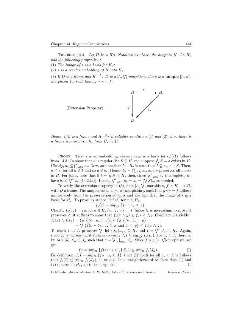
Chapter 14. Regular Completions 134
Theorem 14.4. Let H be a HA. Notation as above, the diagram H∗−→ H∗
has the following properties :
(1) The image of ∗ is a basis for H∗;
(2) ∗ is a regular embedding of H into H∗.
(3) If D is a frame and Hf−→ D is a [∧,
∨]-morphism, there is a unique [∧,
∨]-
morphism f∗, such that f∗ ∗ = f .
(Extension Property)
D
H
?
- H∗
f
∗
f∗
Hence, if Ω is a frame and Hh−→ Ω satisfies conditions (1) and (2), then there is
a frame isomorphism h∗ from H∗ to Ω.
Proof. That ∗ is an embedding whose image is a basis for cI(H) followsfrom 14.3. To show that ∗ is regular, let S ⊆ H and suppose
∧S = b exists in H.
Clearly, b∗ ⊆⋂s∈S s∗. Now, assume that I ∈ H∗ is such that I ⊆ s∗, s ∈ S. Then,
a ≤ s, for all a ∈ I and so a ∈ b∗. Hence, b∗ =⋂s∈S s∗, and ∗ preserves all meets
in H. For joins, note that if b =∨S in H, then, since
∨∗s∈S s∗ is complete, we
have b∗ ∈∨∗
s∗ (14.2.(a)). Hence,∨∗
s∈S s∗ = b∗ = (∨S)∗, as needed.
To verify the extension property in (3), fix a [∧,∨
]-morphism, f : H −→ D,with D a frame. The uniqueness of a [∧,
∨]-morphism g such that g ∗ = f follows
immediately from the preservation of joins and the fact that the image of ∗ is abasis for H∗. To prove existence, define, for x ∈ H∗,
f∗(x) = supD fa : a∗ ≤ x.Clearly, f∗(a∗) = fa, for a ∈ H, i.e., f∗ ∗ = f . Since f∗ is increasing, to prove itpreserves ∧, it suffices to show that f∗(x ∧ y) ≥ f∗x ∧ f∗y. Corollary 8.4 yields
f∗(x) ∧ f∗(y) = (∨fa : a∗ ⊆ x) ∧ (
∨fb : b∗ ⊆ y
=∨f(a ∧ b) : a∗ ⊆ x and b∗ ⊆ y ≤ f∗(x ∧ y).
To check that f∗ preserves∨
, let Jαα∈A ⊆ H∗ and I =∨∗
Jα in H∗. Again,since f∗ is increasing, it suffices to verify f∗I ⊆ supD f∗(Iα). For a∗ ⊆ I, there is,by 14.2.(a), Sα ⊆ Jα such that a =
∨ ⋃α∈A Sα. Since f is a [∧,
∨]-morphism, we
get
fa = supD f(s) : s ∈⋃Sα ≤ supD f∗(Jα). (I)
By definition, f∗I = supD fa : a∗ ⊆ I; since (I) holds for all a∗ ⊆ I, it followsthat f∗(I) ≤ supD f∗(Jα), as needed. It is straightforward to show that (1) and(2) determine H∗, up to isomorphism.
F. Miraglia. An Introduction to Partially Ordered Structures and Sheaves. Logica no Aviao.
Chapter 14. Regular Completions 135
The frame H∗ is called the completion of H. All we will ever need to know
about H∗ are the properties of the diagram H∗−→ H∗ in Theorem 14.4.
Example 14.5. The statement of 14.4 is best possible : we cannot hope toget a complete extension to H∗ of a complete morphism H −→ D. Indeed, let H= [−1, 0) ∪ (0, 1] ⊆ R, with its natural order. It is easily established that
H∗ = [−1, 1] = H ∪ 0.Let D = [0, 1] ∪ [2, 3]; define H
f−→D as the gluing of two linear, strictly increasingmaps, one from [−1, 0) onto [0, 1), and the other from (0, 1] onto (2, 3]. Note thatf is a regular embedding of H into D; f has only two extensions to H∗ : one taking0 to 1 and the other, mapping 0 to 2. The only one that is a [∧,
∨]-morphism is
the former, but it does not preserve infinite meets. 2
For Boolean algebras, Theorem 14.4 yields
Corollary 14.6. If B is a Boolean algebra, then the frame B∗ is a cBa andwe have
(1) B∗−→ B∗ is a regular embedding.
(2) The image of ∗ is a basis for B∗.
(3) If A is a cBa and Bf−→ A is a [∧,
∨]-morphism, there is a unique complete
morphism, B∗f∗−→ A, such that f∗ ∗ = f .
Moreover, if A is a cBa and Bh−→ A is a diagram satisfying (1) and (2), then
there is a unique isomorphism h∗, from B∗ onto A, such that h∗ ∗ = h.
Remark 14.7. One may ask if “BA-morphism” may be substituted for“[∧,
∨]-morphism” in item (3) of Corollary 14.6. The answer is no. To explain
what is involved, we succinctly comment on free objects in categories of algebras.For more details, consult [34] (Chapter I.4) or [3], particularly Chapters I and V.
Let L be a first order language with equality, but possessing no relation symbolsother than equality; let τ be the type of L. A model for L is called an algebraof type τ . The concept of morphism is clear : a map between two algebras of thesame type that preserve all the operations in L. Clearly, the identity mapping isa morphism and composition of morphisms – defined as the usual composition ofmaps –, is a morphism. We have a category, Algτ , of algebras of type τ . It is clearthat Algτ has products for any family of objects.
Definition 14.8. Let K be a class of algebras in Algτ and S a set. An algebra
F is the free algebra generated by S over K if there is a map Sf−→ F , such that
for all algebras B in K and all maps Sg−→ B, there is a unique morphism in
Algτ , Fh−→ B, such that h f = g.
F. Miraglia. An Introduction to Partially Ordered Structures and Sheaves. Logica no Aviao.

Chapter 14. Regular Completions 136
B
S
?
- F
h
f
g
An algebra is free over K if it is the algebra freely generated by some set over K.
A class K inAlgτ is an an equational class iff K is closed under the followingoperations :
(i) Taking isomorphic copies of homomorphic images of members of K;
(ii) Taking isomorphic copies of subalgebras of members of K;
(iii) Taking isomorphic copies of direct products of members of K.
K is trivial if it consists of the one element algebras of Algτ .
The classes of lattices, distributive lattices, Heyting and Boolean algebras,groups, rings, etc., are all non-trivial equational classes (but not all of the sametype). There is an important result of G. Birkhoff guaranteeing that a class ofalgebras in Algτ is equational iff it consists of all models of the universal closureof a set of atomic formulas in L. For equational classes we can state
Theorem A. (Thm. I.12.4, [3]) Let K be a non-trivial equational class. Then, foreach set S, the free algebra generated by S over K exists and belongs to K.
Theorem A guarantees the existence of free objects in any of the categories(lattices, HAs, BAs, etc.) mentioned above.
The free BA or the free HA on a set S is a familiar object : they are the algebrasof propositions, constructed by taking S as the set of atomic propositions, underthe equivalence relation “provably equivalent” from the axioms of the Classical orthe Heyting Propositional Calculus.
In contrast to Theorem A, we have (see [34] or [72])
Theorem B. (Gaifmann; Hales; Solovay) There is no free complete Booleanalgebra on a countable number of generators.
Consequently, there is no cBa BN and a map N g−→ BN, such that for all cBas
D and functions N f−→ D, there is a unique complete morphism BNh−→ D,
satisfying h g = f .
We now see that “[∧,∨
]-morphism” cannot be substituted by “BA-morphism”in Corollary 14.6.(3). If it were possible, then the completion of the free BA gen-erated by N would be the free cBa generated by N, contradicting Theorem B.
It is possible, however, to extend BA-morphisms with values in a completeBoolean algebra. This result is important and its precise formulation will appearin the next Chapter. 2
F. Miraglia. An Introduction to Partially Ordered Structures and Sheaves. Logica no Aviao.

Chapter 14. Regular Completions 137
For frames and their morphisms, the situation is quite distinct from that de-scribed by Theorem B in 14.7, as shown by Theorem 14.9 below, due to Benabou.
If X is a set, the family of finite subsets of X, Fin(X), is a poset underinclusion, in fact a lattice with ⊥ but without > (unless X is finite). Write ΩX forthe frame of opens of the U-topology of 8.3 on Fin(X). We have
Theorem 14.9. Notation as above, let Xι−→ ΩX be given by ι(x) = x→.
Then, for all frames L and maps g : X −→ L, there is a unique frame morphism,g : ΩX −→ L, making the following diagram commutative :
X - ΩX
g g
L
ι
AAAAAAU
Hence, ΩX is the free frame generated by X.
Proof. Write∧
, ∧,∨
, ∨ for meets and joins in L. If α ∈ Fin(X), then
α→ =⋂x∈α x→ =
⋂x∈α ι(x).
We define
(*) g(α→) =∧x∈α gx.
Note that for x ∈ X, (*) yields g(ι(x)) = gx, and the displayed diagram in thestatement is commutative. If α, β ∈ Fin(X), then
α→ ∩ β→ = (α ∪ β)→,
and so
(**)
g(α→ ∩ β→) = g((α ∪ β)→) =∧x∈(α∪β) ι(x)
=∧x∈α ι(x) ∧
∧y∈β ι(y)
= g(α→) ∧ g(β→).It follows immediately from (**) that
(***) α→ ⊆ β→ ⇒ g(α→) ≤ g(β→).
To extend g to U ∈ ΩX , write U =⋃i∈I α
→i and set
g(U) =∨i∈I g(α→i ).
To see that g is well defined, first note that if β→ ⊆ U , then the supercom-pactness of β→ (8.3.(ii)) entails the existence of i ∈ I such that β→ ⊆ α→i . Hence,(***) yields
g(β→) ≤ g(α→i ) ≤ g(U).
It now straightforward that if U =⋃j∈J β
→j , then∨
i∈I g(α→i ) =∨j∈J g(β→j ),
and g is indeed well defined. If U =⋃α∈S α
→ and V =⋃β∈T β
→, with S, T ⊆Fin(X), then 8.4, applied in ΩX , yields
F. Miraglia. An Introduction to Partially Ordered Structures and Sheaves. Logica no Aviao.

Chapter 14. Regular Completions 138
U ∩ V =⋃〈α,β〉∈S×T α→ ∩ β→.
But then from (**) and 8.4 in L we get
g(U ∩ V ) =∨〈α,β〉∈S×T g(α→ ∩ β→) =
∨〈α,β〉∈S×T g(α→) ∧ g(β→)
= g(U) ∧ g(V ),
showing that g preserves finite meets. The preservation of arbitrary joins is straight-forward. Uniqueness is clear from the construction.
Exercises
14.10. Let H be a HA and D be the filter of dense elements in H. Notationas in 14.4 and 10.5, let H∗ be the completion of H and write D∗ for the filter ofdense elements in H∗.
a) There is a unique injective BA-morphism, ∗ : H/D −→ H∗/D∗, making thefollowing diagram commutative :
H/D
H
?
- H∗
πD
∗
H∗/D∗
πD∗
∗?
-
b) H∗/D∗ is the completion of H/D 1. 2
The exercises that follow describe the MacNeille completion and its relationto the completions we have presented above. A slightly different account of thissame construction, using closure operators, can be found in section 2 of ChapterXII of [3], under the name of normal completion.
14.11. Let (P,≤) be a poset. All notation is as in Definition 2.6 and thecomments right after it.
A cut in P is a pair of subsets of P , (A,B) such that A ⊆ B← and B ⊆ A→.Every element x of P gives rise to a cut, c(x) = (x←, x→). Let cP be the set of allcuts in P , partially ordered by
(A,B) ≤ (C,D) iff A ⊆ C (or equivalently, iff D ⊆ B).
We denote by c : P −→ cP the map x 7→ c(x).
a) A cut (A,B) is equal to c(x), for some x ∈ P , iff A ∩ B 6= ∅.b) cP is a complete lattice and c is a regular embedding of P in cP . 2
14.12. Notation as in 14.11, assume that P is lattice.
a) If (A,B) is a cut in P , then A is an ideal and B a filter in P .
b) If P is a HA (BA), then cP is a frame (resp., cBa), isomorphic to the completionP∗ of Theorem 14.4 (resp., Corollary 14.6). 2
1In the notation of 14.6, H∗/D∗ = (H/D)∗.
F. Miraglia. An Introduction to Partially Ordered Structures and Sheaves. Logica no Aviao.

CHAPTER 15
Extension of Morphisms
We prove here that BA-morphisms with values in a complete Boolean algebracan be extended to BAs containing its domain, an important result due to S.Sikorski.
If B is a BA, it is readily verified that the intersection of any family of subal-gebras of B is again a subalgebra of B. Thus, if S is a subset of B, we can definethe subalgebra generated by S in B, as
[S] =⋂B′ : B′ is a subalgebra of B and S ⊆ B′.
Recall that for a, b in B, a 4 b (the symmetric difference of a and b) is definedin 5.5 as
a 4 b = (a ∧ ¬ b) ∨ (b ∧ ¬ a).
Lemma 15.1. Let B be a BA, B′ a subalgebra of B and m an element of B.Then
a) The subalgebra H generated by B′ and m is given by
H = (a ∧ m) ∨ (b ∧ ¬m): a, b ∈ B′.b) For all x, y, t, z in B′, the following are equivalent :
i) x ∧ m = t ∧ m and y ∧ ¬m = t ∧ ¬m.
ii) (x ∧ m) ∨ (y ∧ ¬m) = (t ∧ m) ∨ (z ∧ ¬m).
iii) x 4 t ≤ ¬m and y 4 z ≤ m.
Proof. a) It is straightforward to show that the left hand side of the equationis a subalgebra of B, and so it must the least one containing B′ and m.
b) It is immediate that (i) implies (ii), while taking the intersection of the equalitiesin (ii) with m and ¬m yields (ii).
(i) ⇒ (iii) : The first equation in (i) yields x ∧ m ∧ ¬ t = ⊥, and so x ∧ ¬ t ≤¬m. Similarly, t ∧ ¬x ≤ ¬m, and x 4 t ≤ ¬m. The other inequality stated in(iii) is proven similarly.
(iii) ⇒ (i) : From x 4 t ≤ ¬m we get
x ∧ ¬ t ∧ m = t ∧ ¬x ∧ m = ⊥.
Thus, x ∧ m ≤ t and t ∧ m ≤ x. But then, x ∧ m = t ∧ m. The remaining equalityin (i) is obtained analogously.
139

Chapter 15. Extension of Morphisms 140
With these preliminaries we have
Theorem 15.2. Let B be a BA and let B′ a subalgebra of B. If B is a cBa,any BA-morphism from B′ to B can be extended to a BA-morphism from B to B.
Proof. We may assume that B′ is a proper subalgebra of B. We also fix aBA-morphism f from B′ to B. As a first step, we prove
Fact. For m ∈ B, let H the BA generated in B by B′ and m. Then f can beextended to a BA morphism from H to B.
Proof. Let S = m← ∩ B′ and T = m→ ∩ B′; clearly every element of S is lessthan or equal to any element of T . Since f is increasing and B is complete, weconclude that ∨
f(S) ≤∧f(T ).
Let w be any element of B such that∨f(S) ≤ w ≤
∧f(T ). Using Lemma 15.1(a),
define g : H −→ B, by
g([a ∧ m] ∨ [b ∧ ¬m]) = (fa ∧ w) ∨ (fb ∧ ¬w),
where a, b ∈ B′. It must be shown that g is well defined; if x, y, t, z are elementsof B′ such that
(x ∧ m) ∨ (y ∧ ¬m) = (t ∧ m) ∨ (z ∧ ¬m),
then by 15.1.(b) we have (x 4 t) ≤ ¬m and (y 4 z) ≤ m. Thus, (y 4 z) ∈ S and¬ (x 4 t) ∈ T . Hence, since f is a BA morphism, we get
f(y 4 z) = fy 4 fz ≤ w and w ≤ f(¬ (x 4 t)) = ¬ f(x 4 t),
that is, fx 4 ft ≤ ¬w. But these are exactly the conditions needed to have
(fx ∧ w) ∨ (fy ∧ ¬w) = (ft ∧ w) ∨ (fz ∧ ¬w),
and g is well defined. Clearly, g is a BA morphism and the Fact is proven.
Consider
V = H g−→ B :H a subalgebra of B, B′ ⊆ H,
g is a BA-morphism and g|B′ = f ,
partially ordered by “extension”, i.e., g ≤ h iff dom g ⊆ dom h and h|domg = g. V
satisfies the conditions of Zorn’s Lemma (2.20), and has a maximal element g. Toend the proof, note that if dom g where a proper subalgebra of B, then the Factwould provide a proper extension of g, contradicting its maximality.
Theorem 15.2 is analogous to many other extension results, like the Hahn-Banach Theorem in Functional Analysis. In fact, there are significant relationsbetween these results. We refer the interested reader to [8] and [18].
Corollary 15.3. A complete Boolean algebra B satisfies the following uni-versal properties :
[BA− inj] Let B′f−→ B be a BA monomorphism. Then, for any BA-morphism
B′h−→ B, there is a BA-morphism B
g−→ B, such that g f = h.
F. Miraglia. An Introduction to Partially Ordered Structures and Sheaves. Logica no Aviao.

Chapter 15. Extension of Morphisms 141
[HA− inj] Let H and H ′ be Heyting algebras and H ′f−→ H be a HA-
monomorphism. Then, for any HA-morphism H ′h−→ B, there is a
HA-morphism Hg−→ B, such that g f = h.
B
H ′
?
- H
h
f
g
Proof. Property [BA − inj] follows immediately from Theorem 15.2. Forthe Heyting algebra case, let D and D′ be the filter of dense elements in H and H ′,respectively; by 6.21, f induces an injective BA-morphism from H ′/D′ to H/D,while h induces a BA-morphism from H ′/D′ to B. By [BA−inj], the map inducedby h can be extended to H/D; the required HA-morphism g is the composition ofthis extension with the quotient map H −→ H/D.
With 15.3 we can generalize, in one direction, 14.6.(3) :
Corollary 15.4. Let B be a BA and B∗−→ B∗ be the completion of B. If
B is a cBa and Bf−→ B is a BA morphism, then there exists a BA morphism,
f∗ : B∗ −→ B, such that f∗ ∗ = f . Moreover, if f is a monomorphism, the sameis true of f∗.
Proof. The only statement still to verify is that f∗ is monic if f is monic.Let c 6= d ∈ B∗; the injectivity of f∗ equivalent to f∗(c 4 d) 6= ⊥. Since B is abasis for B∗, there is a 6= ⊥ in B such that ⊥ < a∗ ≤ c 4 d. But then, from
f∗(c) 4 f∗(d) = f∗(c 4 d) ≥ f∗(a∗) = fa,
and the injectivity of f , it is clear that f∗(c 4 d) 6= ⊥, as needed.
In the language of Category Theory (see 16.5), Corollary 15.3 tells us thatcomplete Boolean algebras are injective objects both in the category of Booleanalgebras and in the category of Heyting algebras. The converse of these statementsis also true (see Exercise 15.5). Corollary 15.4 guarantees that the completion ofa BA B is the injective hull of B, that is, a minimal injective object containingB, as set down in item (d) of Definition 16.36.
Exercises
15.5. Prove that a BA (HA) is injective in the category of BAs (resp., HAs)iff it is a complete Boolean algebra. The definition of injective is “satisfies theuniversal properties [BA− inj] and [HA− inj]” in the statement of 15.3. 2
F. Miraglia. An Introduction to Partially Ordered Structures and Sheaves. Logica no Aviao.
Part 2
Category Theory
CHAPTER 16
Categorical Constructions
In this chapter we collect most of the language of Category Theory used inthe text. It is not a substitute for the reading of [44] or [53], but is included asa convenient reference for the reader. Many of the basic constructions are alsodescribed in chapter I of [3].
1. Categories and Morphisms
Definition 16.1. A category A is a pair 〈Ob(A), M(A) 〉 where Ob(A) isa class, whose elements are the objects of A and M(A) is a class, which is adisjoint union (1.5)
M(A) =∐
(A,B)∈Ob(A) [A,B]A,
where [A,B]A is a (possibly empty) set, called the set of morphisms from A toB in A. Whenever A is clear from context, we write [A,B] in place of [A,B]A.Moreover, for each triple of objects of A, 〈A,B,C 〉, we have a map
[A,B] × [B,C] −→ [A,C], 〈 f, g 〉 7→ g f ,
called composition, which satisfies the following conditions :
[ 1] : Composition, whenever defined, is associative.
[ 2] : For A ∈ Ob(A), there is IdA in [A,A], such that for B ∈ Ob(A), f ∈ [A,B]and g ∈ [B,A],
f IdA = f and IdA g = g.
The morphism IdA is unique, being called the identity of the object A. If f ∈ [A,B],we say that A is the domain of f (domf = A) and that B is the codomain of f(codomf = B). We use standard functional notation for morphisms. Hence,
f : A −→ B, Af−→ B,
are synonymous with f ∈ [A,B].
A category is small if the class of its objects is a set; it is said to be set basedif all its objects are sets and all its morphisms are set-theoretical maps.
Definition 16.2. Let A, B be categories. B is a subcategory of A iffOb(B) ⊆ Ob(A) and
∀ A, B ∈ Ob(B), [A,B]B ⊆ [A,B]A.
B is a full subcategory of A if [A,B]B = [A,B]A, for all A, B in Ob(B).
143

Chapter 16. Categorical Constructions 144
Remark 16.3. Here is a list of categories, some of which we have alreadymentioned, that will be of standard use :
∗ Set, the category of sets and mappings;
∗ Po, the category of partially ordered sets and increasing maps;
∗ L, the category of lattices and lattice morphisms;
∗ D, the category of distributive lattices and lattice morphisms;
∗ HA, the category of Heyting algebras and HA-morphisms;
∗ BA, the category of Boolean algebras and BA-morphisms;
∗ Frame, the category of frames and frame morphisms;
∗ cBa, the category of cBas, with complete morphisms;
∗ Framep, the category of frames with enough points and frame morphisms;
∗ Top, the category of Topological spaces and continuous maps;
∗ Htop, the category of Hausdorff spaces and continuous maps;
∗ CTop, the category of compact Hausdorff spaces and continuous maps;
∗ Sob, the category of sober spaces and continuous maps.
∗ Algτ , the category of algebras of type τ (see 14.7). 2
Example 16.4. Let 〈P,≤〉 be a poset. We construct a category, also writtenP , by setting Ob(P ) = P and for x, y ∈ P ,
[x, y] =
〈x, y 〉 if x ≤ y
∅ otherwise
Composition is clear: if x ≤ y ≤ z, 〈 y, z 〉 〈x, y 〉 = 〈x, z 〉. Clearly, 〈x, x 〉 = Idx,for all x ∈ P . Hence, every poset has a natural structure of category. 2
Example 16.5. To every category A corresponds a dual category, writtenAop, defined as follows :
∗ Ob(Aop) = Ob(A); ∗ For A, B ∈ Ob(A), [A,B]Aop = [B,A]A.
Clearly, (Aop)op = A. Thus, all theorems about categories embodies two results: ifa statement S holds in A, then its dual holds in Aop. Moreover, if the hypothesisused to prove S, also hold in Aop, then its dual is true in A = (Aop)op. 2
Example 16.6. Let A be a category and let A be an object in A. We definetwo categories, AA and AA, as follows :
[AA 1] : The objects of AA are morphisms in A, f : A −→ B, with B ∈ Ob(A);
[AA 2] : If I = (Af−→ B) and J = (A
g−→ C) are objects in AA, then a morphism
in AA, Ih−→ J , is a morphism h ∈ [B,C]A, such that h f = g.
A - B
g h
C
f
AAAAAU
B - C
β γ
A
η
AAAAAU
F. Miraglia. An Introduction to Partially Ordered Structures and Sheaves. Logica no Aviao.
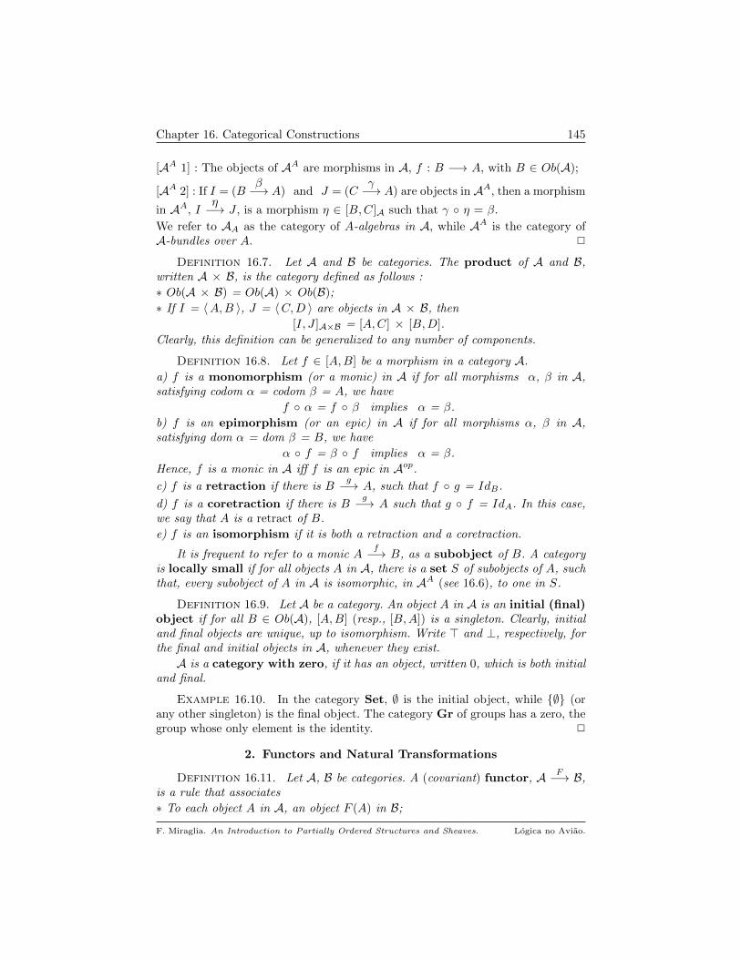
Chapter 16. Categorical Constructions 145
[AA 1] : The objects of AA are morphisms in A, f : B −→ A, with B ∈ Ob(A);
[AA 2] : If I = (Bβ−→ A) and J = (C
γ−→ A) are objects in AA, then a morphism
in AA, Iη−→ J , is a morphism η ∈ [B,C]A such that γ η = β.
We refer to AA as the category of A-algebras in A, while AA is the category ofA-bundles over A. 2
Definition 16.7. Let A and B be categories. The product of A and B,written A × B, is the category defined as follows :
∗ Ob(A × B) = Ob(A) × Ob(B);
∗ If I = 〈A,B 〉, J = 〈C,D 〉 are objects in A × B, then
[I, J ]A×B = [A,C] × [B,D].
Clearly, this definition can be generalized to any number of components.
Definition 16.8. Let f ∈ [A,B] be a morphism in a category A.
a) f is a monomorphism (or a monic) in A if for all morphisms α, β in A,satisfying codom α = codom β = A, we have
f α = f β implies α = β.
b) f is an epimorphism (or an epic) in A if for all morphisms α, β in A,satisfying dom α = dom β = B, we have
α f = β f implies α = β.
Hence, f is a monic in A iff f is an epic in Aop.
c) f is a retraction if there is Bg−→ A, such that f g = IdB.
d) f is a coretraction if there is Bg−→ A such that g f = IdA. In this case,
we say that A is a retract of B.
e) f is an isomorphism if it is both a retraction and a coretraction.
It is frequent to refer to a monic Af−→ B, as a subobject of B. A category
is locally small if for all objects A in A, there is a set S of subobjects of A, suchthat, every subobject of A in A is isomorphic, in AA (see 16.6), to one in S.
Definition 16.9. Let A be a category. An object A in A is an initial (final)object if for all B ∈ Ob(A), [A,B] (resp., [B,A]) is a singleton. Clearly, initialand final objects are unique, up to isomorphism. Write > and ⊥, respectively, forthe final and initial objects in A, whenever they exist.
A is a category with zero, if it has an object, written 0, which is both initialand final.
Example 16.10. In the category Set, ∅ is the initial object, while ∅ (orany other singleton) is the final object. The category Gr of groups has a zero, thegroup whose only element is the identity. 2
2. Functors and Natural Transformations
Definition 16.11. Let A, B be categories. A (covariant) functor, A F−→ B,is a rule that associates
∗ To each object A in A, an object F (A) in B;
F. Miraglia. An Introduction to Partially Ordered Structures and Sheaves. Logica no Aviao.

Chapter 16. Categorical Constructions 146
∗ To each morphism f ∈ [A,B]A, a morphism F (f) ∈ [F (A), F (B)]B, such that
(1) F (IdA) = IdF (A); (2) F (f g) = F (f) F (g),
where A ∈ Ob(A) and f , g are morphisms with codom g = dom f . Notice that forall A, B ∈ Ob(A), F induces a map
[A,B]A −→ [F (A), F (B)]B, f 7→ F (f).
F is faithful if this map is injective and full if it is onto.
A contravariant functor, G : A −→ B, is a functor from Aop to B.If F : A −→ B and G : B −→ C are functors, their composition is a functor,(G F ) : A −→ C, given by
∗ If A ∈ Ob(A), (G F )(A) = G(F (A));
∗ If Af−→ B is a morphism in A, (G F )(f) = G(F (f)).
Example 16.12. If A is a category, IdA for the identity functor from A toA, i.e., the functor that associates every object and morphism in A to itself. 2
Example 16.13. If A is a set based category, the forgetful functor from Ato Set is the functor that associates to every object in A its underlying set andto each morphism in A its underlying map. In general, if A and B are categories,and A has “richer” structure than B, there is a forgetful functor from A to B,which forgets the richer structure in A. As examples, we mention:
(1) LetL be the category of lattices and Po be the category of posets. The forgetfulfunctor from L to Po associates to each lattice its underlying poset and to eachlattice morphism the same map considered just as an increasing function.
(2) The forgetful functor from the category D, of distributive lattices, to thecategory L.
(3) The forgetful functor from the category of BAs, BA, to the category of HAs,HA, associates to each BA its underlying HA structure (x → y = ¬x ∨ y) andto each BA-morphism the corresponding map as a HA-morphism. 2
Example 16.14. Let A be a category. An object A in A determines twofunctors from A to Set, hA and hA, defined as follows :
[hA 1] : For each B ∈ Ob(A), hA(B) = [A,B], the set of morphismsfrom A to B in A.
[hA 2] : For a morphism Bg−→ C in A, hA(g) : [A, B] −→ [A, C] is given by
f 7−→ g f .
A - B
g f g
C
f
AAAAAAU
B - C
f g f
A
g
AAAAAAU
F. Miraglia. An Introduction to Partially Ordered Structures and Sheaves. Logica no Aviao.

Chapter 16. Categorical Constructions 147
[hA 1] : For each B ∈ Ob(A), hA(B) = [B,A], the set of morphisms from B to Ain A.
[hA 2] : For a morphism Bg−→ C in A, hA(g) : [C, A] −→ [B, A] is given by
f 7→ f g.
Note that hA is covariant, while hA is contravariant. These functors are called themorphism functors with parameter A. 2
Remark 16.15. Let A, B and C be categories. A functor from A × B to Cis usually called a bifunctor; it can have distinct variances in each coordinate.For example, it might be covariant in the first and contravariant in the second.Actually, all possible combinations can occur.
Note that if F : A −→ B and G : C −→ D are functors, then we have abifunctor,
T ≡ F × G : A × B −→ C × D,
which on objects is given by T (A, B) = 〈F (A), G(B) 〉, and on morphisms isdefined by T (f , g) = 〈F (f), G(g) 〉. Clearly, these observations can be generalizedto any number of components. 2
Example 16.16. Let F : A −→ B and G : B −→ A be functors of the samevariance. We shall assume, without loss of generality, that they are both covariant.These functors give rise to bifunctors
Fh, hG : Aop × B −→ Set,
defined as follows :
∗ For A ∈ Ob(A) and B ∈ Ob(B),Fh(A,B) = [F (A), B]B
hG(A,B) = [A, G(B)]A.
∗ For a morphism 〈 f, g 〉 : 〈A,B 〉 −→ 〈C,D 〉 in Aop × B,Fh(f, g) : [F (A), B] −→ [F (C), D], given by h 7→ g h F (f).
hG(f, g) : [A,G(B)] −→ [C,G(D)], given by h 7→ G(g) h f.
F (C)
F (A)
6
- B
F (f)
h
D
g
Fh(f, g)
?- C
A
6
- G(B)
f
h
G(D)
G(g)
hG(f, g)
?-
We shall return to this example when we discuss adjointness. 2
Morphisms of functors are called natural transformations :
F. Miraglia. An Introduction to Partially Ordered Structures and Sheaves. Logica no Aviao.

Chapter 16. Categorical Constructions 148
Definition 16.17. Let F , G : A −→ B be functors, of the same variance 1.A natural transformation, η : F −→ G, is a family of morphisms in B,
η = ηA ∈ [F (A), G(A)] : A ∈ Ob(A),such that if A
f−→ B is a morphism in A, the following diagram is commutative :
G(B)
F (A)
?
- G(A)
F (f)
ηA
F (B)
G(f)
ηB
?- G(A)
F (B)
?
- G(B)
F (f)
ηB
F (A)
G(f)
ηA
?-
where the diagram on the right is for the case in which F and G are contravariant.When ηA is an isomorphism for each A ∈ Ob(A), η is said to be a natural
equivalence. Natural transformations can be composed, as follows : if Fη−→ G
and Gµ−→ T are natural transformations, then π : F −→ T , given by
π = µA ηA : A ∈ Ob(A),is the composition µ η. Write [F,G] for the class of natural transformations fromF to G.
Definition 16.18. Let A be a category. A covariant functor F : A −→ Setis representable if there is A ∈ Ob(A) such that F is naturally equivalent to hA.
A fundamental result concerning representable functors is :
Theorem 16.19. (The Yoneda Lemma) Let F : A −→ Set be a functor,where A is a category. Then,
a) For any object A in A, there is a bijection
ηA,F : [hA, F ] −→ F (A), ηAF (η) = ηA(IdA),
which is natural in F and A.
b) If A and B are objects in A, the function
ηA,C : [hA, hC ] −→ [C,A], θA,C(η) = ηA(IdA),
is a bijection, which is natural in both A and C.
For a proof, see Lemma in pg. 61 of [44] or Lemma 2.1 and Corollary 2.2, pg.97ff, in [53].
3. Adjoint functors and Equivalence of Categories
Definition 16.20. Notation as 16.16, two functors A F−→ B and B G−→ A arean adjoint pair, (F,G), if there is a natural equivalence of set-valued bifunctors,η : Fh −→ hG. Thus, for each object 〈A,B 〉 ∈ Ob(Aop × B), we have a naturalbijective correspondence
1I.e., both covariant or both contravariant.
F. Miraglia. An Introduction to Partially Ordered Structures and Sheaves. Logica no Aviao.
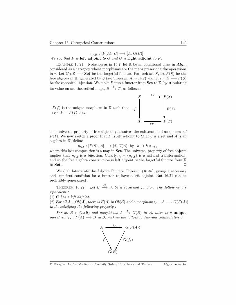
Chapter 16. Categorical Constructions 149
ηAB : [F (A), B] −→ [A, G(B)].
We say that F is left adjoint to G and G is right adjoint to F .
Example 16.21. Notation as in 14.7, let K be an equational class in Algτ ,considered as a category whose morphisms are the maps preserving the operationsin τ . Let G : K −→ Set be the forgetful functor. For each set S, let F (S) be thefree algebra in K, generated by S (see Theorem A in 14.7) and let ιS : S −→ F (S)be the canonical injection. We make F into a functor from Set to K, by stipulating
its value on set-theoretical maps, Sf−→ T , as follows :
F (f) is the unique morphism in K such thatιT F = F (f) ιS .
T
S
?
- F (S)
f
ιS
F (T )
F (f)
ιT
?-
The universal property of free objects guarantees the existence and uniqueness ofF (f). We now sketch a proof that F is left adjoint to G. If S is a set and A is analgebra in K, define
ηSA : [F (S), A] −→ [S, G(A)] by h 7→ h ιS ,
where this last composition is a map in Set. The universal property of free objectsimplies that ηSA is a bijection. Clearly, η = ηSA is a natural transformation,and so the free algebra construction is left adjoint to the forgetful functor from Kto Set. 2
We shall later state the Adjoint Functor Theorem (16.35), giving a necessaryand sufficient condition for a functor to have a left adjoint. But 16.21 can beprofitably generalized :
Theorem 16.22. Let B G−→ A be a covariant functor. The following areequivalent :
(1) G has a left adjoint.
(2) For all A ∈ Ob(A), there is F (A) in Ob(B) and a morphism ιA : A −→ G(F (A))in A, satisfying the following property :
For all B ∈ Ob(B) and morphisms Af−→ G(B) in A, there is a unique
morphism f∗ : F (A) −→ B in B, making the following diagram commutative :
A - G(F (A))
f G(f∗)
G(B)
ιA
AAAAAU
F. Miraglia. An Introduction to Partially Ordered Structures and Sheaves. Logica no Aviao.

Chapter 16. Categorical Constructions 150
Proof. Generalize the argument in Example 16.21.
Definition 16.23. Let A be a subcategory of B. A is a reflective subcategoryof B if the natural embedding A −→ B has a left adjoint R, called the reflectionfunctor from B to A. A is a coreflective subcategory of B if the natural embed-ding A −→ B has a right adjoint, called the coreflection of B in A.
Example 16.24. a) The following are full reflective categories of Top 2 :
∗ The category of Ti spaces, i = 1, 2, 3 (1.20);
∗ The category of completely regular spaces;
∗ the category of totally disconnected spaces;
b) The category of normal spaces (1.20) is a reflective subcategory of Htop.
c) The full subcategory of torsion-free groups is reflective in Ab, the category ofAbelian groups.
d) The full subcategory Ab of Abelian groups is reflective in the category ofgroups, Gr.
e) The full subcategory of torsion groups in Ab is an example of a coreflectivesubcategory. 2
Definition 16.25. Two categories, A and B, are equivalent if there arefunctors, F : A −→ B and G : B −→ A, together with natural equivalences
η : (G F ) −→ IdA and µ : (F G) −→ IdB.
The pair (F,G) is called an equivalence between A and B. A contravariant equiv-alence is called a duality.
An example of duality is presented in 12.17 : that between Sob and Framep.We shall see other important examples in the chapters ahead.
4. Diagrams and Limits
Definition 16.26. Let A be a category and let D be a small category. AD-diagram in A is a functor D : D −→ A.
If B is a subcategory of D, we write D|B for the B-diagram obtained by applying
D just to the objects and arrows in B.
The notion of diagram is functorial, that is, if F : A −→ B is a functor and Dis a D-diagram in A, then F D is a D-diagram in B.
Example 16.27. Let A be a category.
(1) Let D be the category consisting of two objects (1) and (2), such that [(1), (2)]has two distinct elements. A D-diagram in A consists of parallel arrows in A,
A --
f
g
B ,
with A, B ∈ Ob(A) and f , g ∈ [A, B].
2The category of topological spaces and continuous maps.
F. Miraglia. An Introduction to Partially Ordered Structures and Sheaves. Logica no Aviao.
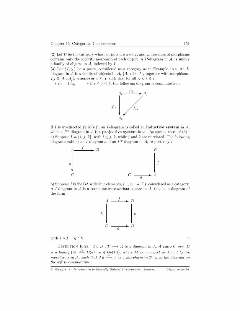
Chapter 16. Categorical Constructions 151
(2) Let D be the category whose objects are a set I, and whose class of morphismscontains only the identity morphism of each object. A D-diagram in A, is simplya family of objects in A, indexed by I.
(3) Let 〈 I,≤〉 be a poset, considered as a category as in Example 16.4. An I-diagram in A is a family of objects in A, Ai : i ∈ I, together with morphisms,fij ∈ [Ai, Aj ], whenever i ≤ j, such that for all i, j, k ∈ I∗ fii = IdAi ; ∗ If i ≤ j ≤ k, the following diagram is commutative :
Ak
Ai
?
- Aj
fik
fij
fjk
If I is up-directed (2.26(ii)), an I-diagram is called an inductive system in A,while a Iop-diagram in A is a projective system in A. As special cases of (3) :
a) Suppose I = i, j, k, with i ≤ j, k, while j and k are unrelated. The followingdiagrams exhibit an I-diagram and an Iop-diagram in A, respectively :
C
A
?
- B
g
f
C
B
A
f
g
?-
b) Suppose I is the BA with four elements, ⊥, a, ¬ a, >, considered as a category.A I-diagram in A is a commutative covariant square in A, that is, a diagram ofthe form
C
A
?
- B
h
f
D
k
g
?-
with k f = g h. 2
Definition 16.28. Let D : D −→ A be a diagram in A. A cone C over D
is a family M fd−→ D(d) : d ∈ Ob(D), where M is an object in A and fd are
morphisms in A, such that if dα−→ d′ is a morphism in D, then the diagram on
the left is commutative :
F. Miraglia. An Introduction to Partially Ordered Structures and Sheaves. Logica no Aviao.
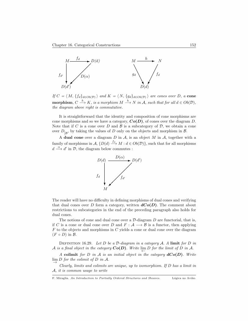
Chapter 16. Categorical Constructions 152
D(d′)
M
?
- D(d)
fd′
fd
D(α)
M - N
gd fd
D(d)
h
AAAAAU
If C = 〈M, fdd∈Ob(D) 〉 and K = 〈N, gdd∈Ob(D) 〉 are cones over D, a cone
morphism, Ch−→ K, is a morphism M
h−→ N in A, such that for all d ∈ Ob(D),the diagram above right is commutative.
It is straightforward that the identity and composition of cone morphisms arecone morphisms and so we have a category, Co(D), of cones over the diagram D.Note that if C is a cone over D and B is a subcategory of D, we obtain a coneover D|B, by taking the values of D only on the objects and morphism in B.
A dual cone over a diagram D in A, is an object M in A, together with a
family of morphisms in A, D(d)fd−→M : d ∈ Ob(D), such that for all morphisms
dα−→ d′ in D, the diagram below commutes :
M
D(d)
?
- D(d′)
fd
D(α)
fd′
The reader will have no difficulty in defining morphisms of dual cones and verifyingthat dual cones over D form a category, written dCo(D). The comment aboutrestrictions to subcategories in the end of the preceding paragraph also holds fordual cones.
The notions of cone and dual cone over a D-diagram D are functorial, that is,if C is a cone or dual cone over D and F : A −→ B is a functor, then applyingF to the objects and morphisms in C yields a cone or dual cone over the diagram(F D) in B.
Definition 16.29. Let D be a D-diagram in a category A. A limit for D inA is a final object in the category Co(D). Write lim← D for the limit of D in A.
A colimit for D in A is an initial object in the category dCo(D). Writelim→ D for the colimit of D in A.
Clearly, limits and colimits are unique, up to isomorphism. If D has a limit inA, it is common usage to write
F. Miraglia. An Introduction to Partially Ordered Structures and Sheaves. Logica no Aviao.
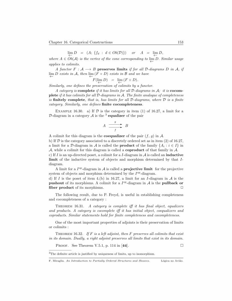
Chapter 16. Categorical Constructions 153
lim← D = (A; fd : d ∈ Ob(D)) or A = lim← D,
where A ∈ Ob(A) is the vertex of the cone corresponding to lim← D. Similar usage
applies to colimits.
A functor F : A −→ B preserves limits if for all D-diagrams D in A, iflim← D exists in A, then lim← (F D) exists in B and we have
F (lim← D) = lim← (F D).
Similarly, one defines the preservation of colimits by a functor.
A category is complete if it has limits for all D-diagrams in A; it is cocom-plete if it has colimits for all D-diagrams in A. The finite analogue of completenessis finitely complete, that is, has limits for all D-diagrams, where D is a finitecategory. Similarly, one defines finite cocompleteness.
Example 16.30. a) If D is the category in item (1) of 16.27, a limit for aD-diagram in a category A is the 3 equalizer of the pair
A --
f
g
B
A colimit for this diagram is the coequalizer of the pair (f , g) in A.
b) If D is the category associated to a discretely ordered set as in item (2) of 16.27,a limit for a D-diagram in A is called the product of the family Ai : i ∈ I inA, while a colimit for this diagram is called a coproduct of that family in A.
c) If I is an up-directed poset, a colimit for a I-diagram in A is called an inductivelimit of the inductive system of objects and morphism determined by that I-diagram.
A limit for a Iop-diagram in A is called a projective limit for the projectivesystem of objects and morphism determined by the Iop-diagram.
d) If I is the poset of item 4.(b) in 16.27, a limit for an I-diagram in A is thepushout of its morphisms. A colimit for a Iop-diagram in A is the pullback orfiber product of its morphisms. 2
The following result, due to P. Freyd, is useful in establishing completenessand cocompleteness of a category :
Theorem 16.31. A category is complete iff it has final object, equalizersand products. A category is cocomplete iff it has initial object, coequalizers andcoproducts. Similar statements hold for finite completeness and cocompleteness.
One of the most important properties of adjoints is their preservation of limitsor colimits :
Theorem 16.32. If F is a left adjoint, then F preserves all colimits that existin its domain. Dually, a right adjoint preserves all limits that exist in its domain.
Proof. See Theorem V.5.1, p. 114 in [44].
3The definite article is justified by uniqueness of limits, up to isomorphism.
F. Miraglia. An Introduction to Partially Ordered Structures and Sheaves. Logica no Aviao.
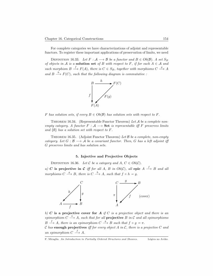
Chapter 16. Categorical Constructions 154
For complete categories we have characterizations of adjoint and representablefunctors. To register these important applications of preservation of limits, we need
Definition 16.33. Let F : A −→ B be a functor and B ∈ Ob(B). A set SBof objects in A is a solution set of B with respect to F , if for each A ∈ A and
each morphism Bf−→ F (A), there is C ∈ SB, together with morphisms C
g−→ A
and Bh−→ F (C), such that the following diagram is commutative :
F (A)
B
?
- F (C)
f
h
F (g)
F has solution sets, if every B ∈ Ob(B) has solution sets with respect to F .
Theorem 16.34. (Representable Functor Theorem) Let A be a complete non-empty category. A functor F : A −→ Set is representable iff F preserves limitsand ∅ has a solution set with respect to F .
Theorem 16.35. (Adjoint Functor Theorem) Let B be a complete, non-emptycategory. Let G : B −→ A be a covariant functor. Then, G has a left adjoint iffG preserves limits and has solution sets.
5. Injective and Projective Objects
Definition 16.36. Let C be a category and A, C ∈ Ob(C).
a) C is projective in C iff for all A, B in Ob(C), all epic Af−→ B and all
morphisms Cg−→ B, there is C
h−→ A, such that f h = g.
A
C
h
B
g
f
?-
A
C
?
- B
π
g
f (cover)
b) C is a projective cover for A if C is a projective object and there is an
epimorphism Cπ−→ A, such that for all projective B in C and all epimorphisms
Bf−→ A, there is an epimorphism C
g−→ B such that f g = π.
C has enough projectives iff for every object A in C, there is a projective C and
an epimorphism Cf−→ A.
F. Miraglia. An Introduction to Partially Ordered Structures and Sheaves. Logica no Aviao.
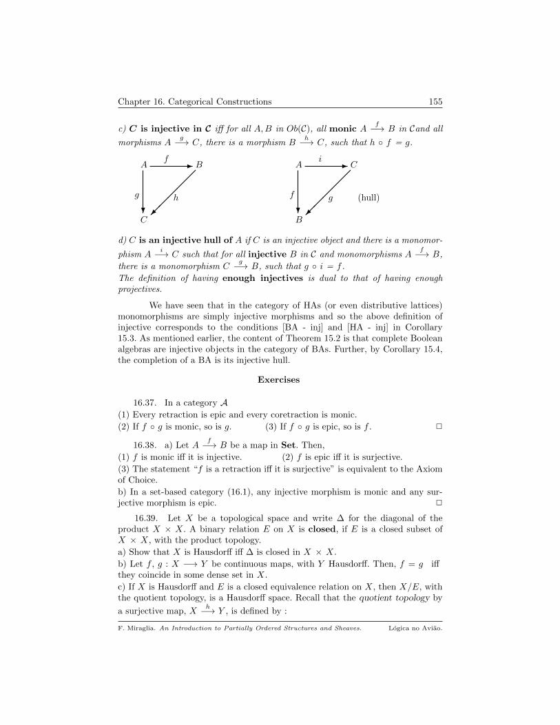
Chapter 16. Categorical Constructions 155
c) C is injective in C iff for all A,B in Ob(C), all monic Af−→ B in Cand all
morphisms Ag−→ C, there is a morphism B
h−→ C, such that h f = g.
C
A
?
- B
g
f
h
B
A
?
- C
f
i
g (hull)
d) C is an injective hull of A if C is an injective object and there is a monomor-
phism Ai−→ C such that for all injective B in C and monomorphisms A
f−→ B,
there is a monomorphism Cg−→ B, such that g i = f .
The definition of having enough injectives is dual to that of having enoughprojectives.
We have seen that in the category of HAs (or even distributive lattices)monomorphisms are simply injective morphisms and so the above definition ofinjective corresponds to the conditions [BA - inj] and [HA - inj] in Corollary15.3. As mentioned earlier, the content of Theorem 15.2 is that complete Booleanalgebras are injective objects in the category of BAs. Further, by Corollary 15.4,the completion of a BA is its injective hull.
Exercises
16.37. In a category A(1) Every retraction is epic and every coretraction is monic.
(2) If f g is monic, so is g. (3) If f g is epic, so is f . 2
16.38. a) Let Af−→ B be a map in Set. Then,
(1) f is monic iff it is injective. (2) f is epic iff it is surjective.
(3) The statement “f is a retraction iff it is surjective” is equivalent to the Axiomof Choice.
b) In a set-based category (16.1), any injective morphism is monic and any sur-jective morphism is epic. 2
16.39. Let X be a topological space and write ∆ for the diagonal of theproduct X × X. A binary relation E on X is closed, if E is a closed subset ofX × X, with the product topology.
a) Show that X is Hausdorff iff ∆ is closed in X × X.
b) Let f , g : X −→ Y be continuous maps, with Y Hausdorff. Then, f = g iffthey coincide in some dense set in X.
c) If X is Hausdorff and E is a closed equivalence relation on X, then X/E, withthe quotient topology, is a Hausdorff space. Recall that the quotient topology by
a surjective map, Xh−→ Y , is defined by :
F. Miraglia. An Introduction to Partially Ordered Structures and Sheaves. Logica no Aviao.
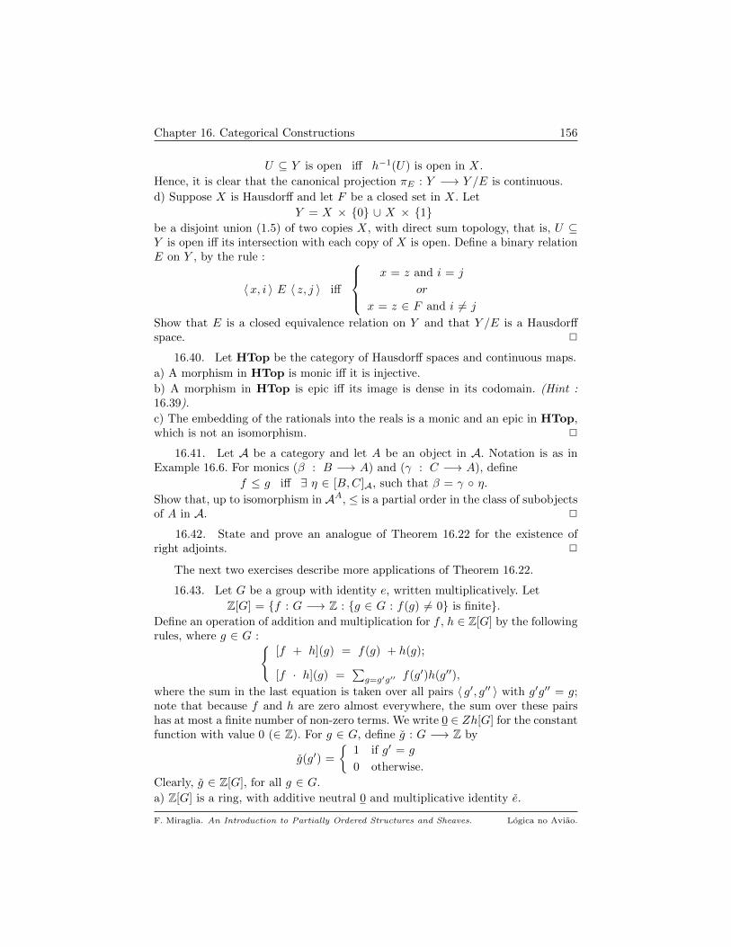
Chapter 16. Categorical Constructions 156
U ⊆ Y is open iff h−1(U) is open in X.
Hence, it is clear that the canonical projection πE : Y −→ Y /E is continuous.
d) Suppose X is Hausdorff and let F be a closed set in X. Let
Y = X × 0 ∪ X × 1be a disjoint union (1.5) of two copies X, with direct sum topology, that is, U ⊆Y is open iff its intersection with each copy of X is open. Define a binary relationE on Y , by the rule :
〈x, i 〉 E 〈 z, j 〉 iff
x = z and i = j
or
x = z ∈ F and i 6= j
Show that E is a closed equivalence relation on Y and that Y /E is a Hausdorffspace. 2
16.40. Let HTop be the category of Hausdorff spaces and continuous maps.
a) A morphism in HTop is monic iff it is injective.
b) A morphism in HTop is epic iff its image is dense in its codomain. (Hint :16.39).
c) The embedding of the rationals into the reals is a monic and an epic in HTop,which is not an isomorphism. 2
16.41. Let A be a category and let A be an object in A. Notation is as inExample 16.6. For monics (β : B −→ A) and (γ : C −→ A), define
f ≤ g iff ∃ η ∈ [B,C]A, such that β = γ η.
Show that, up to isomorphism in AA, ≤ is a partial order in the class of subobjectsof A in A. 2
16.42. State and prove an analogue of Theorem 16.22 for the existence ofright adjoints. 2
The next two exercises describe more applications of Theorem 16.22.
16.43. Let G be a group with identity e, written multiplicatively. Let
Z[G] = f : G −→ Z : g ∈ G : f(g) 6= 0 is finite.Define an operation of addition and multiplication for f , h ∈ Z[G] by the followingrules, where g ∈ G :
[f + h](g) = f(g) + h(g);
[f · h](g) =∑g=g′g′′ f(g′)h(g′′),
where the sum in the last equation is taken over all pairs 〈 g′, g′′ 〉 with g′g′′ = g;note that because f and h are zero almost everywhere, the sum over these pairshas at most a finite number of non-zero terms. We write 0 ∈ Zh[G] for the constantfunction with value 0 (∈ Z). For g ∈ G, define g : G −→ Z by
g(g′) =
1 if g′ = g
0 otherwise.
Clearly, g ∈ Z[G], for all g ∈ G.
a) Z[G] is a ring, with additive neutral 0 and multiplicative identity e.
F. Miraglia. An Introduction to Partially Ordered Structures and Sheaves. Logica no Aviao.
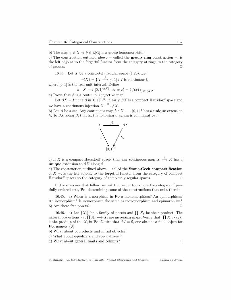
Chapter 16. Categorical Constructions 157
b) The map g ∈ G 7→ g ∈ Z[G] is a group homomorphism.
c) The construction outlined above − called the group ring construction −, isthe left adjoint to the forgetful functor from the category of rings to the categoryof groups. 2
16.44. Let X be a completely regular space (1.20). Let
γ(X) = X f−→ [0, 1] : f is continuous,where [0, 1] is the real unit interval. Define
β : X −→ [0, 1]γ(X), by β(x) = 〈 f(x) 〉f∈γ(X).
a) Prove that β is a continuous injective map.
Let βX = Image β in [0, 1]γ(X); clearly, βX is a compact Hausdorff space and
we have a continuous injection Xβ−→ βX.
b) Let A be a set. Any continuous map h : X −→ [0, 1]A has a unique extensionh∗ to βX along β, that is, the following diagram is commutative :
X - βX
h h∗
[0, 1]A
β
AAAAAU
c) If K is a compact Hausdorff space, then any continuous map Xh−→ K has a
unique extension to βX along β.
d) The construction outlined above − called the Stone-Cech compactificationof X −, is the left adjoint to the forgetful functor from the category of compactHausdorff spaces to the category of completely regular spaces. 2
In the exercises that follow, we ask the reader to explore the category of par-tially ordered sets, Po, determining some of the constructions that exist therein.
16.45. a) When is a morphism in Po a monomorphism? An epimorphism?An isomorphism? Is isomorphism the same as monomorphism and epimorphism?
b) Are there free posets? 2
16.46. a) Let Xi be a family of posets and∏
Xi be their product. Thenatural projections πi :
∏Xi −→Xi are increasing maps. Verify that (
∏Xi, πi)
is the product of the Xi in Po. Notice that if I = ∅, one obtains a final object forPo, namely ∅.b) What about coproducts and initial objects?
c) What about equalizers and coequalizers ?
d) What about general limits and colimits? 2
F. Miraglia. An Introduction to Partially Ordered Structures and Sheaves. Logica no Aviao.

CHAPTER 17
Limits and Colimits of First-Order Structures
Since most of our applications of limits and colimits are for diagrams of first-order structures over a poset, we include some basic results for this case. Weassume that the reader is familiar with the fundamental notions of Logic andModel Theory, in particular of the concept of satisfaction. Classic references are[38], [39], [68]; [71] has an interesting approach to first-order logic. It should besaid that Theorems 17.10, 17.15 and Corollary 17.18 are part of the folklore ofModel Theory.
1. First-Order Languages and Logic
We recall the construction of a first-order language L with equality.
17.1. Alphabet of L. ∗ A set vn : n ∈ N of variable symbols;
∗ The logical symbols ∧ (and), ∨ (or), → (implies) and ¬ (negation);
∗ The quantifiers ∃ (existential) and ∀ (universal);
∗ A binary relation symbol =, for equality;
∗ For each integer n ≥ 1,
(i) A set rel(n,L) of n-ary relation symbols;
(ii) A set op(n,L) of n-ary operation symbols;
(iii) A set Ct(L) of constants symbols. 2
17.2. Terms. Defined by induction on complexity, as follows :
∗ Variables and constant are terms;
∗ If n ≥ 1 is an integer, t1, . . . , tn are terms in L and ω ∈ op(n), then ω(t1, . . . , tn)is a term. 2
17.3. Formulas. Defined by induction on complexity, where n ≥ 1 is aninteger :
∗ If R ∈ rel(n) and t1, . . . , tn are terms in L, R(t1, . . . , tn) is a formula, called anatomic formula;
∗ If φ, ψ are formulas in L and 3 is one of the logical symbols ∧, ∨ or →, then(φ 3 ψ) is a formula.
∗ If φ is a formula, then ¬φ (the negation of φ) is a formula;
∗ If φ is a formula and vn is a variable, then ∀ vn φ and ∃ vn φ are formulas. 2
17.4. Basic Notions. a) To every formula φ in L is associated a sequenceof formulas, of lesser complexity, that describe the process of constructing φ from
158

Chapter 17. Limits and Colimits of First-Order Structures 159
the atomic formulas. The formulas in this sequence are called subformulas of φ.The occurrences of a variable vn in φ are divided into two categories :
(1) bound, when vn occurs in a subformula of φ of the type Qvn ψ, where Q =∃, ∀;(2) free, when the occurrence is not bound.
b) (Substitution) If φ is a formula, vn is a variable and τ is a term, write φ( pτ | vnq )for the formula obtained by substituting all free occurrences of vn in φ by τ .
c) If t is a term and φ is a formula in L, write t(v1, . . . , vn), φ(v1, . . . , vn) to meanthat the free variables in t and φ are among the ones being displayed. As usual,write v for the sequence 〈 v1, . . . , vn 〉; we may also use, as is standard, x, x, y, yand z, z to name variables.
d) A term t is free for vn in a formula φ iff in φ( pt | vnq ) (see (b) above) novariable in t becomes bound.
e) A formula φ in L is
∗ A sentence if it has no free variables. Let Sent(L) be the set of sentences in L;
∗ quantifier-free if there is no quantifier occurs in φ;
∗ positive if implication and negation do not occur in φ;
∗ existential if it is of the form ∃xψ, where ψ is quantifier-free;
∗ universal if it is of the form ∀xψ, where ψ is quantifier-free;
∗ primitive if it is of the form ∃xφ, where φ is a conjunction of atomic formulas;
∗ ∀ ∃ if is of the form ∀x ∃ y ψ, where ψ is quantifier-free;
∗ Horn if it is of the form ∀x [(ψ1 ∧ . . . ∧ ψn) → ψ], where ψ, ψ1, . . . , ψn areatomic formulas.
The reader should have no trouble in recognizing the content of expressions like“positive-existential” or “positive ∀∃”. 2
17.5. The Intuitionistic Predicate Calculus,H. The following is a Hilbertstyle 1 formalization of the Intuitionistic Predicate Calculus2, written H :
If φ, ψ and χ are formulas in L, v is a variable and τ is a term :
1. φ → (ψ → φ);
2. (φ → ψ) → ((φ → (ψ → χ)) → (φ → χ));
3. φ → (ψ → φ ∧ ψ);
4. φ ∧ ψ → φ;
5. φ ∧ ψ → ψ;
6. φ → (φ ∨ ψ);
7. ψ → (φ ∨ ψ);
8. (φ → χ) → ((ψ → χ) → (φ ∨ ψ → χ));
9. (φ → ψ) → ((φ → ¬ψ) → ¬φ);
10. ¬φ → (φ → ψ).
1For Gentzen style formalizations, see [58], [39], [38].2Due to A. Heyting.
F. Miraglia. An Introduction to Partially Ordered Structures and Sheaves. Logica no Aviao.
Chapter 17. Limits and Colimits of First-Order Structures 160
11. If τ is a term free for v in φ 3,
11.a. ∀v φ → φ( pτ | vq );
11.b. φ( pτ | vq ) → ∃v φ,
where φ( pτ | vq ) denotes substitution of τ for v in φ, as in 17.4.(b).
12. Deduction rules :
Modus Ponens :φ, φ → ψ
ψ
∀-rule :
φ → ψ(v)φ → ∀v ψ(v)
∃-rule :ψ(v)→ φ∃v ψ(v) → φ,
where in the ∀-rule and the ∃-rule v must not occur free in φ.
The axioms for equality are the usual ones, including the Leibniz substitution rule
[L] : If τ is a term in L, free for a variable v in φ, then 4
φ(v) ∧ (v = τ) → φ( pτ | vq ).
The first ten schemata, together with Modus Ponens formalize the IntuitionisticPropositional Calculus. To obtain the Classical Calculus, add (or replace axiom10 by) the rule
10C . ¬¬φ → φ.
where φ is any formula in L. In [65] one will find a different and interesting proposalfor the formalization of the Intuitionistic Predicate Calculus.
If Γ ∪ φ is a set of formulas in L, a proof of φ from Γ consists of a sequenceof formulas ψ1, . . . , ψn in L, such that ψn is φ and satisfying, for 1 ≤ k ≤ n,
∗ ψk ∈ Γ or ∗ ψk is an axiom or
∗ ψk comes from earlier formulas in the sequence, through the use of one of thededuction rules.
We writeΓ `H φ If φ is a consequence of Γ in H;
Γ `C φ If φ is a consequence of Γ in the Classical Calculus.
It is clear that Γ `H φ ⇒ Γ `C φ.
A theorem of H is a formula φ such that ∅ `H φ, written `H φ.
A set of sentences Σ is a theory in H, if it is closed under deduction that is
Σ `H σ ⇒ σ ∈ Σ.
Similarly, one defines the notion of theory in the classical Calculus. 2
On the basic results about these systems is
Proposition 17.6. (Deduction Theorem) Let Γ ∪ σ, φ be a set of formulasin L. If σ is a sentence in L, then
Γ, σ `H φ iff Γ `H (σ → φ).
A similar statement holds for the relation `C .
One of the basic discoveries of Lindenbaum and Tarski is that the syntax offormal theories generates interesting algebraic structures. If φ, ψ are formulas inL, define a relation
3As in 17.4.(d).4It is enough to assume this just for function and relation symbols in L.
F. Miraglia. An Introduction to Partially Ordered Structures and Sheaves. Logica no Aviao.
Chapter 17. Limits and Colimits of First-Order Structures 161
φ ≡ ψ iff `H (φ → ψ) ∧ (ψ → φ).
This is an equivalence relation on L and the set of its equivalence classes is theLindenbaum algebra of L. For intuitionistic systems − propositional or first-order −, the Lindenbaum algebra of L is Heyting algebra. For classical systems,it is a Boolean algebra. The propositional case is important, in particular becausetheir Lindenbaum algebras furnish the free objects in the categories of Heytingand Boolean algebras. For more information on this topic, see [59] and [60].
2. First-order Structures and their Morphisms
Since we shall be constantly using sequences, all the notational conventions in1.4 will be of constant use.
Let L be a first-order language with equality as in the previous section. AL-structure is a set M , together with
∗ For R ∈ rel(n,L) a subset RM ⊆ Mn, called the interpretation of R in M ;
∗ For ω ∈ op(n,L), a map ωM : Mn −→ M , the interpretation of ω in M ;
∗ For c ∈ Ct(L), an element cM ∈ M , the interpretation of c in M ;
∗ The equality symbol is interpreted as the diagonal of the M2.
By induction on complexity, a term t(v1, . . . , vn), in the free variables v1, . . . , vn,induces a map, tM : Mn −→ M , called the interpretation of t in M .
We shall assume the reader familiar with the concept of interpretation of aformula φ(v1, . . . , vn) in M (see [7]) and the symbol
M |= φ[a],
read φ holds in M at a ∈ Mn.
The main notions of morphism of L-structures are recalled in
Definition 17.7. Let L be a first-order language with equality and let M , Nbe structures for L. Let f : M −→ N be a map.
a) f is a L-morphism if for all integers n ≥ 1
(i) If c ∈ Ct, then f(cM ) = cN .
(ii) If ω ∈ op(n) and x ∈ Mn, f(ωM (x)) = ωN (f(x));
(iii) If R ∈ rel(n) and x ∈ Mn, then M |= R[x] ⇒ N |= R[f(x)].
b) f is a L-embedding if it is a L-morphism such that for all n ≥ 1, R ∈ rel(n)and x ∈ Mn M |= R[x] ⇔ N |= R[f(x)].
c) f is an elementary embedding if for all formulas φ(v1, . . . , vn) in L andx ∈ Mn, M |= φ[x] iff N |= φ[f(x)].
When clear from context, L will be omitted from the notation. L-structures andL-morphism are a category, written L-mod.
Remark 17.8. (1) Since equality is in rel(2), embeddings are injective.
(2) If f is a L-morphism and τ(v1, . . . , vn) is a term in L, then
For all x ∈ Mn, f(τM (x)) = τN (f(x)).
(3) Let φ ≡ R(τ1(v1, . . . , vn), . . . , τm(v1, . . . , vn)) be an atomic formula in L andlet f be a map satisfying (i) and (ii) in 17.7.(a). Then, f is a L-morphism iff
For all x ∈ Mn, M |= φ[x] ⇒ N |= φ[f(x)].
F. Miraglia. An Introduction to Partially Ordered Structures and Sheaves. Logica no Aviao.
Chapter 17. Limits and Colimits of First-Order Structures 162
Furthermore, f is an embedding iff
For all x ∈ Mn, M |= φ[x] ⇔ N |= φ[f(x)]. 2
17.9. Products in L-mod. Let Mi, i ∈ I, be a family of L-structures.Let M =
∏i∈I Mi be their set-theoretic product (1.4). M is endowed with a
L-structure, defined coordinatewise as follows, where n ≥ 1 is an integer :
∗ If c ∈ Ct, cM = 〈 cMi 〉i∈I ;∗ If ω ∈ op(n), and 〈 s1, . . . , sn 〉 ∈ Mn, then
ωM (s1, . . . , sn) = 〈ωMi(s1(i), s2(i), . . . , sn(i)) 〉i∈I ;∗ If R ∈ rel(n) and s ∈ Mn, then
M |= R[s] iff ∀ i ∈ I, Mi |= R[s1(i), s2(i), . . . , sn(i)].
Note that the canonical projections, πi : M −→ Mi, are L-morphisms. This con-struction is the product of the Mi in the category L-mod.
Induction on complexity yields :
a) If τ(v1, . . . , vn) is a term in L and s ∈ Mn, then
τM (s) = 〈 τMi(s1(1), . . . , sn(i)) 〉i∈I .b) If φ(v1, . . . , vn) is an atomic formula in L and x ∈ Mn, then
M |= φ[s] iff ∀ i ∈ I, Mi |= φ[s1(i), . . . , sn(i)]. 2
3. Limits in L-mod
Theorem 17.10. Let L be a first-order language with equality, containing atleast one constant symbol and let 〈 I,≤〉 be a poset.
a) The category L-mod is complete.
b) Let D be an I-diagram in L-mod and let lim← D be its limit. Then,
(1) If J ⊆ I is down-cofinal in I, lim← D|J is isomorphic to lim← D.
(2) Let σ ∈ Sent(L) be logically equivalent to a finite conjunction of sentences ofthe form ∀x (∀yψ → φ), where ψ and φ are positive and quantifier free 5. Then,
i ∈ I : D(i) |= σ is down-cofinal in I ⇒ lim← D |= σ.
Proof. a) We make use of Theorem 16.31, verifying that L-mod has finalobject, equalizers and products; by 17.9, it has products.
Equalizers : Let D = (A --
f
g
B) be L-morphisms. Set
E = a ∈ A : f(a) = g(a).For all constants c in L, cE =def cA ∈ E. Moreover, if ω ∈ op(n) is an n-aryoperation symbol in L and a = 〈 a1, . . . , an 〉 ∈ En, then
f(ωA(a)) = ωB(f(a)) = ωB(g(a)) = g(ωA(a)),
and E is closed under the restriction of the interpretations of all operation symbolsin A. For a n-ary relation symbol R in L, set RE = R ∩ En. Then, the canon-ical injection, η : E −→ A is a L-embedding. Moreover, since f η = g η,
5Defined in 17.4.
F. Miraglia. An Introduction to Partially Ordered Structures and Sheaves. Logica no Aviao.
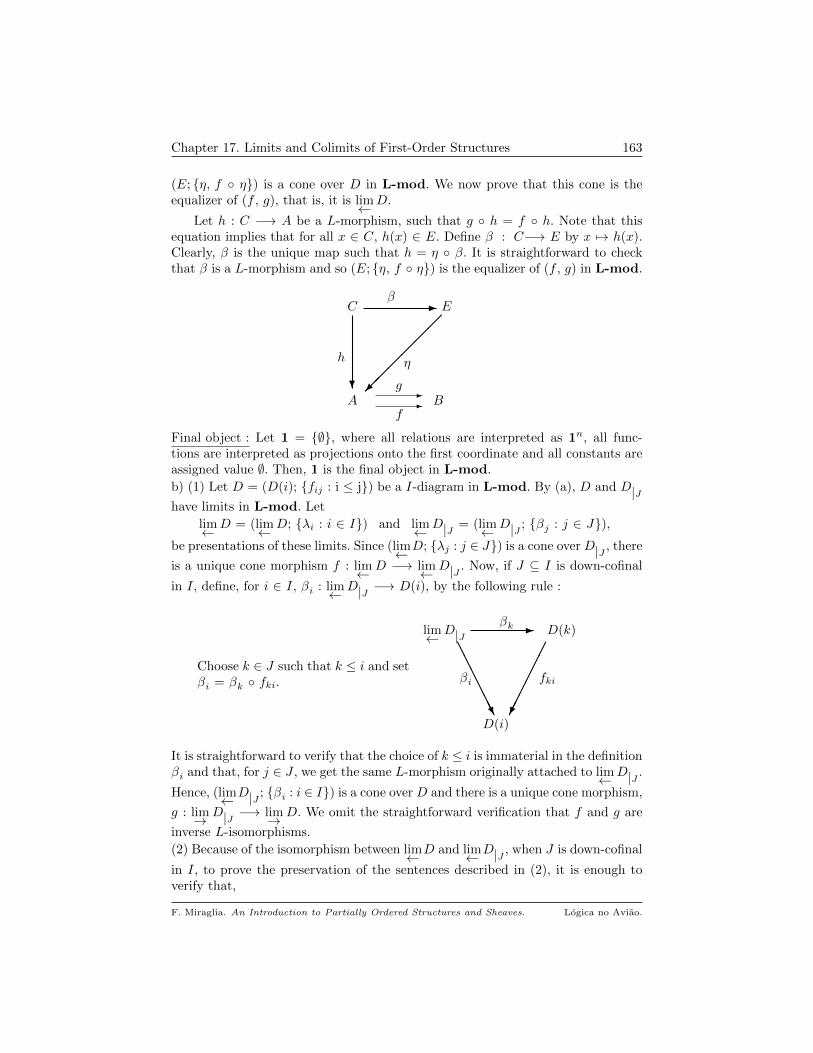
Chapter 17. Limits and Colimits of First-Order Structures 163
(E; η, f η) is a cone over D in L-mod. We now prove that this cone is theequalizer of (f , g), that is, it is lim← D.
Let h : C −→ A be a L-morphism, such that g h = f h. Note that thisequation implies that for all x ∈ C, h(x) ∈ E. Define β : C−→ E by x 7→ h(x).Clearly, β is the unique map such that h = η β. It is straightforward to checkthat β is a L-morphism and so (E; η, f η) is the equalizer of (f , g) in L-mod.
A
C
?
- E
h
β
η
--
f
gB
Final object : Let 1 = ∅, where all relations are interpreted as 1n, all func-tions are interpreted as projections onto the first coordinate and all constants areassigned value ∅. Then, 1 is the final object in L-mod.
b) (1) Let D = (D(i); fij : i ≤ j) be a I-diagram in L-mod. By (a), D and D|Jhave limits in L-mod. Let
lim← D = (lim← D; λi : i ∈ I) and lim← D|J = (lim← D|J ; βj : j ∈ J),be presentations of these limits. Since (lim← D; λj : j ∈ J) is a cone over D|J , there
is a unique cone morphism f : lim← D −→ lim← D|J . Now, if J ⊆ I is down-cofinal
in I, define, for i ∈ I, βi : lim← D|J −→ D(i), by the following rule :
Choose k ∈ J such that k ≤ i and setβi = βk fki.
lim← D|J- D(k)
βi fki
D(i)
βk
AAAAAAU
It is straightforward to verify that the choice of k ≤ i is immaterial in the definitionβi and that, for j ∈ J , we get the same L-morphism originally attached to lim← D|J .
Hence, (lim← D|J ; βi : i ∈ I) is a cone over D and there is a unique cone morphism,
g : lim→ D|J −→ lim→ D. We omit the straightforward verification that f and g are
inverse L-isomorphisms.
(2) Because of the isomorphism between lim← D and lim← D|J , when J is down-cofinal
in I, to prove the preservation of the sentences described in (2), it is enough toverify that,
F. Miraglia. An Introduction to Partially Ordered Structures and Sheaves. Logica no Aviao.

Chapter 17. Limits and Colimits of First-Order Structures 164
If σ is true in all D(i), then it is true in Λ =def lim← D.
Let Σ and Π be the sets of formulas φ(v1, . . . , vn) in L defined by the followingrules :
φ ∈ Σ iff ∀s ∈ Λn, (Λ |= φ[s] iff D(i) |= φ[λi(s)]);
φ ∈ Π iff ∀s ∈ Λn, (D(i) |= φ[λi(s)] ⇒ Λ |= φ[s]).
One then verifies that
∗ All atomic formulas are in Σ; ∗ ψ, φ ∈ Σ ⇒ ψ ∧ φ ∈ Σ;
∗ ψ ∈ Π, φ ∈ Σ ⇒ ∀x ψ ∈ Π and ψ → φ ∈ Π.
Details are left to the reader. Clearly, the desired result follows from the abovestatements.
Remark 17.11. Since L-structures satisfy the laws of Classical Logic, thesentence ∃x(x = x) forces them to be non-empty. If the language L has no con-stants, there are examples where the set of points where two morphisms, withsame domain and codomain, are equal is empty. For these languages, L-mod doesnot have equalizers. Hence, the statement of Theorem 17.10 is sharp. 2
The following characterization of limits of I-diagrams is useful :
Corollary 17.12. Let D = (D(i), fij : i ≤ j) be an I-diagram in L-mod, where I is a poset. Suppose Ct(L) 6= ∅. Let Λ = 〈Λ; λii∈I 〉 be a cone inL-mod over D and let λ =
∏λi be the unique map from Λ to
∏D(i), such that
πi λ = λi, i ∈ I. Then, Λ is (isomorphic to) lim← D iff
[lim 1] : The image of λ in∏D(i) is the set
m ∈∏D(i) : ∀ i, j ∈ I (i ≤ j ⇒ fij(πi(m)) = πj(m).
[lim 2] : For all atomic formulas φ(v1, . . . , vn) in L and s ∈ Λn,
Λ |= φ[s] iff for all i ∈ I, D(i) |= φ[λi(s)].
We now discuss limits for morphisms of I-diagrams in L-mod.
Definition 17.13. Let 〈 I,≤〉 be a poset and
D = (D(i); fij : i ≤ j) and E = (E(i); gij : i ≤ j)be I-diagrams in L-mod. A morphism h : D −→ E consists of a family of L-morphisms, hi : D(i) −→ E(i), i ∈ I, such that for i ≤ j in I, the followingdiagram is commutative :
E(i)
D(i)
?
- D(j)
hi
fij
E(j)
hj
gij
?-
Clearly, IdD = (IdD(i))i∈I is a morphism; if Dh−→ E
k−→ G are morphisms ofI-diagrams, then
F. Miraglia. An Introduction to Partially Ordered Structures and Sheaves. Logica no Aviao.
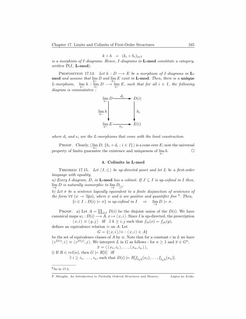
Chapter 17. Limits and Colimits of First-Order Structures 165
k h = (ki hi)i∈Iis a morphism of I-diagrams. Hence, I-diagrams in L-mod constitute a category,written D(I, L-mod).
Proposition 17.14. Let h : D −→ E be a morphism of I-diagrams in L-mod and assume that lim← D and lim← E exist in L-mod. Then, there is a unique
L-morphism, lim← h : lim← D −→ lim← E, such that for all i ∈ I, the following
diagram is commutative :
lim← E
lim← D
?
- D(i)
lim← h
di
E(i)
hi
ei
?-
where di and ei are the L-morphisms that come with the limit construction.
Proof. Clearly, 〈 lim← D; hi di : i ∈ I 〉 is a cone over E; now the universal
property of limits guarantee the existence and uniqueness of lim← h.
4. Colimits in L-mod
Theorem 17.15. Let 〈 I,≤〉 be up-directed poset and let L be a first-orderlanguage with equality.
a) Every I-diagram, D, in L-mod has a colimit. If J ⊆ I is up-cofinal in I then,lim→ D is naturally isomorphic to lim→ D|J .
b) Let σ be a sentence logically equivalent to a finite disjunction of sentences ofthe form ∀x (ψ → ∃yφ), where ψ and φ are positive and quantifier free 6. Then,
i ∈ I : D(i) |= σ is up-cofinal in I ⇒ lim→ D |= σ.
Proof. a) Let A =∐i∈I D(i) be the disjoint union of the D(i). We have
canonical maps wi : D(i) −→ A, x 7→ 〈x, i 〉. Since I is up-directed, the prescription
〈x, i 〉 ≡ 〈 y, j 〉 iff ∃ k ≥ i, j such that fik(x) = fjk(y),
defines an equivalence relation ≡ on A. Let
G = 〈x, i 〉/≡ : 〈x, i 〉 ∈ Abe the set of equivalence classes of A by ≡. Note that for a constant c in L we have〈 cD(i), i 〉 ≡ 〈 cD(j), j 〉. We interpret L in G as follows : for n ≥ 1 and x ∈ Gn,
x = 〈 〈x1, i1 〉, . . . , 〈xn, in 〉 〉,i) If R ∈ rel(n), then G |= R[x] iff
∃ i ≥ i1, . . . , in, such that D(i) |= R[fi1k(x1), . . . , fink(xn)].
6As in 17.4.
F. Miraglia. An Introduction to Partially Ordered Structures and Sheaves. Logica no Aviao.
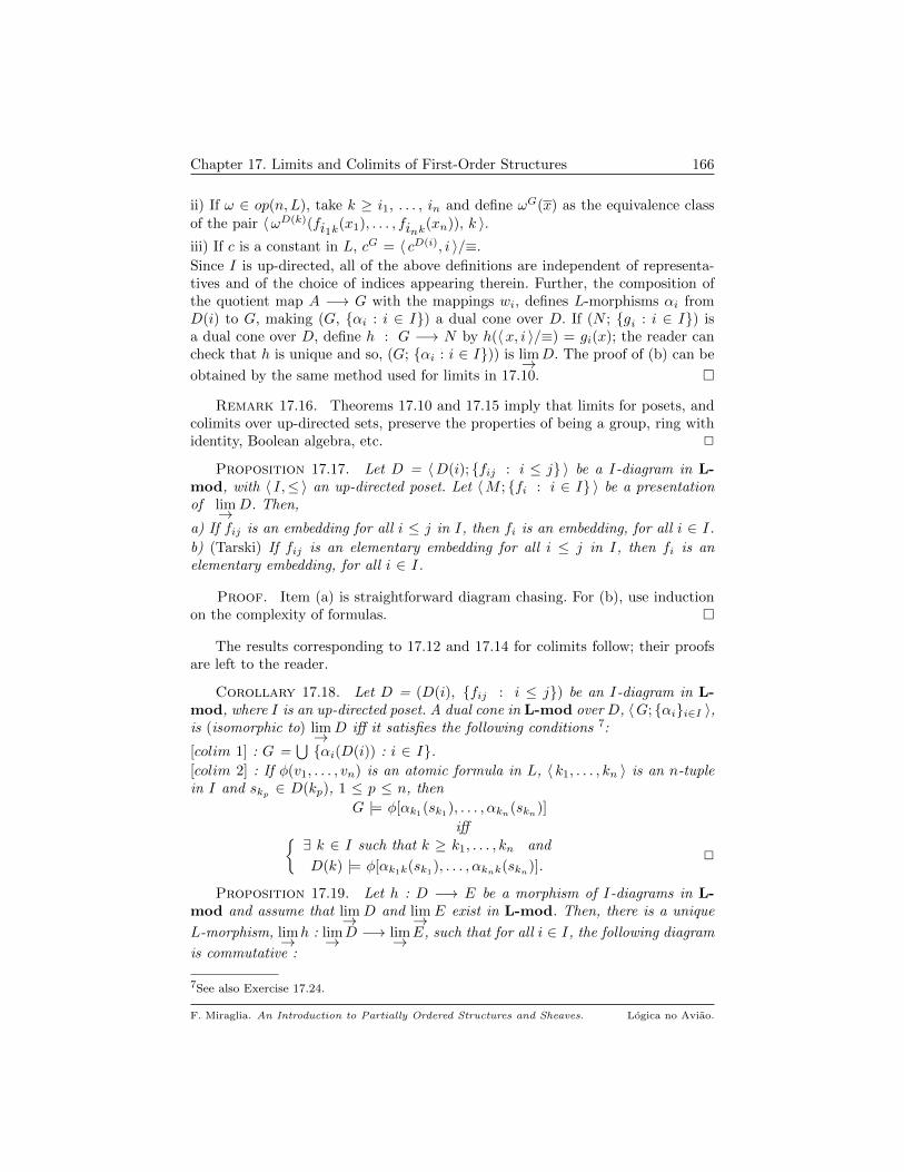
Chapter 17. Limits and Colimits of First-Order Structures 166
ii) If ω ∈ op(n,L), take k ≥ i1, . . . , in and define ωG(x) as the equivalence classof the pair 〈ωD(k)(fi1k(x1), . . . , fink(xn)), k 〉.iii) If c is a constant in L, cG = 〈 cD(i), i 〉/≡.
Since I is up-directed, all of the above definitions are independent of representa-tives and of the choice of indices appearing therein. Further, the composition ofthe quotient map A −→ G with the mappings wi, defines L-morphisms αi fromD(i) to G, making (G, αi : i ∈ I) a dual cone over D. If (N ; gi : i ∈ I) isa dual cone over D, define h : G −→ N by h(〈x, i 〉/≡) = gi(x); the reader cancheck that h is unique and so, (G; αi : i ∈ I)) is lim→ D. The proof of (b) can be
obtained by the same method used for limits in 17.10.
Remark 17.16. Theorems 17.10 and 17.15 imply that limits for posets, andcolimits over up-directed sets, preserve the properties of being a group, ring withidentity, Boolean algebra, etc. 2
Proposition 17.17. Let D = 〈D(i); fij : i ≤ j 〉 be a I-diagram in L-mod, with 〈 I,≤〉 an up-directed poset. Let 〈M ; fi : i ∈ I 〉 be a presentationof lim→ D. Then,
a) If fij is an embedding for all i ≤ j in I, then fi is an embedding, for all i ∈ I.
b) (Tarski) If fij is an elementary embedding for all i ≤ j in I, then fi is anelementary embedding, for all i ∈ I.
Proof. Item (a) is straightforward diagram chasing. For (b), use inductionon the complexity of formulas.
The results corresponding to 17.12 and 17.14 for colimits follow; their proofsare left to the reader.
Corollary 17.18. Let D = (D(i), fij : i ≤ j) be an I-diagram in L-mod, where I is an up-directed poset. A dual cone in L-mod over D, 〈G; αii∈I 〉,is (isomorphic to) lim→ D iff it satisfies the following conditions 7:
[colim 1] : G =⋃αi(D(i)) : i ∈ I.
[colim 2] : If φ(v1, . . . , vn) is an atomic formula in L, 〈 k1, . . . , kn 〉 is an n-tuplein I and skp ∈ D(kp), 1 ≤ p ≤ n, then
G |= φ[αk1(sk1), . . . , αkn(skn)]
iff∃ k ∈ I such that k ≥ k1, . . . , kn and
D(k) |= φ[αk1k(sk1), . . . , αknk(skn)].2
Proposition 17.19. Let h : D −→ E be a morphism of I-diagrams in L-mod and assume that lim→ D and lim→ E exist in L-mod. Then, there is a unique
L-morphism, lim→ h : lim→ D −→ lim→ E, such that for all i ∈ I, the following diagram
is commutative :
7See also Exercise 17.24.
F. Miraglia. An Introduction to Partially Ordered Structures and Sheaves. Logica no Aviao.
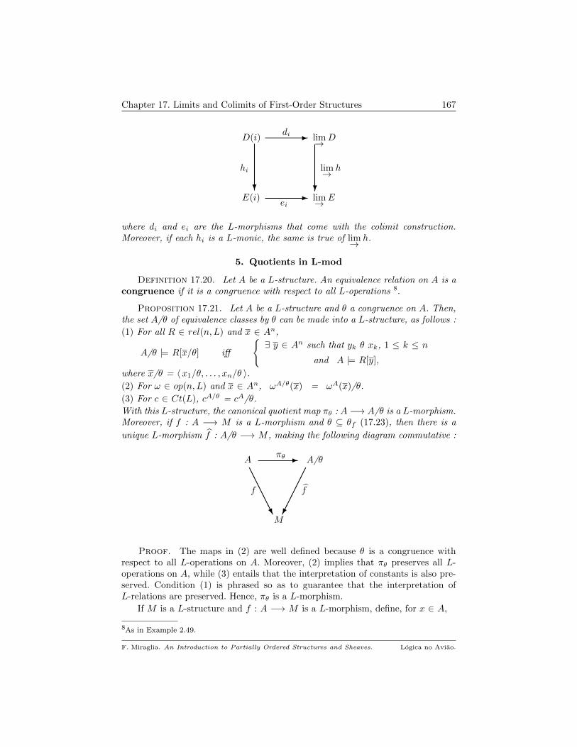
Chapter 17. Limits and Colimits of First-Order Structures 167
E(i)
D(i)
?
- lim→ D
hi
di
lim→ E
lim→ h
ei
?-
where di and ei are the L-morphisms that come with the colimit construction.Moreover, if each hi is a L-monic, the same is true of lim→ h.
5. Quotients in L-mod
Definition 17.20. Let A be a L-structure. An equivalence relation on A is acongruence if it is a congruence with respect to all L-operations 8.
Proposition 17.21. Let A be a L-structure and θ a congruence on A. Then,the set A/θ of equivalence classes by θ can be made into a L-structure, as follows :
(1) For all R ∈ rel(n,L) and x ∈ An,
A/θ |= R[x/θ] iff
∃ y ∈ An such that yk θ xk, 1 ≤ k ≤ n
and A |= R[y],
where x/θ = 〈x1/θ, . . . , xn/θ 〉.(2) For ω ∈ op(n,L) and x ∈ An, ωA/θ(x) = ωA(x)/θ.
(3) For c ∈ Ct(L), cA/θ = cA/θ.
With this L-structure, the canonical quotient map πθ : A −→ A/θ is a L-morphism.Moreover, if f : A −→ M is a L-morphism and θ ⊆ θf (17.23), then there is a
unique L-morphism f : A/θ −→ M , making the following diagram commutative :
A - A/θ
f f
M
πθ
AAAAAU
Proof. The maps in (2) are well defined because θ is a congruence withrespect to all L-operations on A. Moreover, (2) implies that πθ preserves all L-operations on A, while (3) entails that the interpretation of constants is also pre-served. Condition (1) is phrased so as to guarantee that the interpretation ofL-relations are preserved. Hence, πθ is a L-morphism.
If M is a L-structure and f : A −→ M is a L-morphism, define, for x ∈ A,
8As in Example 2.49.
F. Miraglia. An Introduction to Partially Ordered Structures and Sheaves. Logica no Aviao.

Chapter 17. Limits and Colimits of First-Order Structures 168
f(x/θ) = fx.
Since θ ⊆ θf (17.23), f is well defined. If R ∈ rel(n), assume that A/θ |= R[x/θ].Then, there is y ∈ An such that A |= R[y] and xk θ yk, 1 ≤ k ≤ n. Because f isa L-morphism, we conclude that
M |= R[f(y)].
Now xk θ yk and θ ⊆ θf imply that fxk = fyk, 1 ≤ k ≤ n, and so
M |= R[f(x/θ)]
as needed. It is clear that for all constants c in L, f(cA/θ) = cM . For operations
symbols, the argument is analogous. The uniqueness of f is immediate.
The L-structure A/θ in 17.21 is the quotient of A by the congruence θ.
Exercises
17.22. This exercise is related to 22.15 and 22.37. Let H be a HA and F be a(proper) filter in H. For a ∈ H, let Ha = H/a→ be the quotient HA by the filtera→. Write πa : H −→ Ha for the quotient morphism (instead of πa→).
a) F is an up-directed subset of Hop 9.
b) For a ≤ b in H there is a HA-morphism, hba : Hb −→ Ha, making the followingdiagram commutative :
H - Hb
πa hba
Ha
πb
AAAAAU
Moreover, whenever a ≤ b ≤ c, haa = IdHa and hca = hba hcb. Conclude thatF = 〈Ha; hba : a ≤ b in F 〉 is an inductive system of HAs and HA-morphisms.
c) H/F = lim→ F . 2
17.23. If Mf−→ N is a L-morphism, θf = 〈x, y 〉 ∈ M2 : f(x) = f(y)
is a L-congruence on M . 2
17.24. Let D = (D(i), fij : i ≤ j) be an I-diagram in L-mod, where I is anup-directed poset. A dual cone in L-mod over D, 〈G; αii∈I 〉, is (isomorphic to)lim→ D iff it satisfies the following conditions :
[colim 1′] : For all i, j ∈ I, x ∈ D(i) and y ∈ D(j)
αi(x) = αj(y) iff ∃ k ≥ i, j such that fik(x) = fjk(y).
[colim 2′] : For all n-ary relations R in L and ξ ∈ Gn,
M |= R[ξ] ⇔ ∃ k ∈ I and x ∈ D(k)n such that ξ = αk(x) and D(k) |= R[x]. 2
9Recall (2.5) that Hop is H with the opposite order it originally had.
F. Miraglia. An Introduction to Partially Ordered Structures and Sheaves. Logica no Aviao.

Part 3
Spectral Spaces
CHAPTER 18
Boolean Spaces
In this Chapter the results in section 1.2 may be used without explicit refer-ence.
Recall that Ω(X), B(X) and Reg(X) (3.6) denote the frame of opens, the BAof clopens and the cBa of regular opens, respectively, of the topological space X.
Definition 18.1. A T0 topological space X is totally disconnected if B(X)is a basis of opens in X, or equivalently, Ω(X) is a zero-dimensional frame (8.19).A Boolean space is a compact totally disconnected space.
A totally disconnected space X is Hausdorff. For if x 6= y in X, the T0 property(1.20) furnishes an open set U in X, such that x ∈ U and y 6∈ U (or the other wayaround). Since B(X) is a basis of opens in X, we might as well assume that U isclopen, and so x and y have disjoint clopen neighborhoods in X.
A subspace of a totally disconnected space, with the induced topology, is alsototally disconnected, i.e., the property of being totally disconnected is hereditary.A closed subspace of a Boolean space is a Boolean space in its own right.
The following Example describes an important way of obtaining totally dis-connected spaces.
Example 18.2. Let Si, i ∈ I, be a family of sets, considered as topolog-ical spaces with the discrete topology (all points are open). Then, the productS =
∏Si, with the product topology, is totally disconnected. Although a basis
for S appears in 1.25, we introduce new notation that is convenient for dealingwith products of discrete spaces. Recall that ⊆f stands for “finite subset of”.
Let Sω =⋃∏j∈J Sj : J ⊆f I. For s ∈ Sω, define
Vs = f ∈ S : f|doms = s,that is, Vs is the set of extensions of s in S. Then,
V = Vs : s ∈ Sω,is a basis of clopens for the product topology on S.
When each Si is finite, the product topology is compact, by Tychonoff’s The-orem 1.28. In particular, for all A, 2A is a Boolean space, where 2 = 0, 1; thespace 2N is called the Cantor space, being homeomorphic to the Cantor “extractthe middle third” space, a classical construction on the real closed unit interval.
For separable metric spaces, i.e., those possessing a countable dense set,two spaces of this type are fundamental. A result due to Kuratowski asserts that
170

Chapter 18. Boolean Spaces 171
(1) Every complete separable metric space is the continuous image of NN (theBaire space), by a map whose inverse image of each point is at most countable;
(2) The same holds for compact metric spaces, with 2N in place of NN. 2
Lemma 18.3. Let X be a totally disconnected space. Then, X is homeomorphicto a subspace of 2γ , where γ is the weight of X (1.16.(b)). If X is Boolean, thenX is homeomorphic to a closed subspace of 2γ .
Proof. Since the set of cardinals α such that X has a basis of cardinal αhas a least element, fix a basis B = Uβ : β ∈ γ of cardinal γ, which we mayassume to be contained in B(X). Define, for x ∈ X and β ∈ γ,
f : X −→ 2γ , by f(x)(β) =
1 if x ∈ Uβ0 otherwise.
If x 6= y in X, there is β ∈ γ, such that x ∈ Uβ and y 6∈ Uβ . Thus, f(x) 6= f(y)and f is injective; for continuity, let J ⊆f γ and s ∈ 2J ; with notation as in 18.2,Vs is a basic clopen in 2γ , and
f−1(Vs) =⋂β∈J Uβ ,
that is clopen in X. To check that f is open (1.18), let β ∈ γ and set
Vβ = t = 〈 tβ 〉 ∈ 2γ : tβ = 1,a clopen in 2γ . It is immediate from the definition of f that
For all β ∈ γ, f(Uβ) = Vβ ∩ Imf . (I)
For an open set U in X, let K ⊆ γ be such that U =⋃β∈K Uβ . Then, since f is
a bijection between X and its image, (I) yields
f(U) =⋃β∈K Vβ ∩ Imf ,
and f : X −→ Imf is a homeomorphism. If X is compact, the results in Lemma1.24 imply that Imf is a closed subset of 2γ .
Definition 18.4. A Hausdorff space X is dyadic if it is the continuousimage of 2I , for some set I.
Clearly, all dyadic spaces are compact. By the observations (1) and (2) atthe end of 18.2, every compact metric space is dyadic. The class of dyadic spacesis important in the study of functional analytic questions in Banach spaces ofcontinuous functions and in general measure theory.
Lemma 18.3 justifies a closer look at spaces of the type 2A. To deal with topo-logical and combinatorial questions in these spaces, we set down some notation,expanding that already described in 18.2. The posets pFω(A, 2), introduced inExample 2.13 will be of constant use.
Let A be a set; for each s ∈ pFω(A, 2), as in 18.2,
Vs = f ∈ 2A : f|doms = s.When s = 〈 a, 1 〉 or s = 〈 a, 0 〉, a ∈ A, we may write Vs as V(a,1) or V(a,0),respectively. Clearly,
Vs =⋂V(a,s(a)) : a ∈ dom s,
a finite intersection, since doms is finite. The collection
F. Miraglia. An Introduction to Partially Ordered Structures and Sheaves. Logica no Aviao.

Chapter 18. Boolean Spaces 172
B = Vs : s ∈ pFω(A, 2)is a clopen basis for the product topology on 2A. Note that V∅ = 2A. For f ∈ 2A,a fundamental system of neighborhoods of f is given by :
νf = Vs : s = f |B , B ⊆f A.
Recall (2.33, 2.36) that s, t ∈ pFω(A, 2) are up-compatible iff
s|doms∩ domt = t|doms∩ domt;otherwise, s and t are up-incompatible (s ⊥∗ t). Up-compatibility is equivalent tothe existence of x ∈ pFω(A, 2) such that s, t ≤ x. That is, s and t are compatible iffthey have a common extension in pFω(A, 2). We also have that s ⊥∗ t iff t ⊥∗ s.
For s ∈ pFω(A, 2), define
s : doms −→ 2, by s(b) = 1 iff s(b) = 0.
Clearly, s = s. If s, t ∈ pFω(A, 2), then
[⊥∗] s ⊥∗ t iff ∃ ∅ 6= B ⊆ doms ∩ dom t, such that s|B ≤ t.
This condition is symmetric, since s = s.
For up-compatible s, t ∈ pFω(A, 2), it follows from 1.2 that their join, (s ∨ t),exists in pFω(A, 2), being given by
dom (s ∨ t) = doms ∪ dom t;
(s ∨ t)|doms = s and (s ∨ t)|domt = t.
Since sequences with disjoint domains are compatible, their join exist in pFω(A, 2).In particular, if a 6∈ doms, s ∨ 〈 a, 1 〉 and s ∨ 〈 a, 0 〉 are in pFω(A, 2).
If s ∈ pFω(A, 2), define the length of s, l(s), by
[length] l(s) = card(dom s).
The basic properties of the collection B = Vs : s ∈ pFω(A, 2) are in
Lemma 18.5. Let A be a set and s, t ∈ pFω(A, 2). Then,
a) V∅ = 2A. Moreover, Vt ⊆ Vs iff s ≤ t.
b) Vs ∩ Vt 6= ∅ iff s and t are up-compatible and Vs ∩ Vt = V(s∨t).
c) 2A − Vs =⋃Vs|B : B ⊆ dom s, B 6= ∅
=⋃V(a,1−s(a)) : a ∈ dom s.
d) For all a 6∈ dom s,
Vs = V(s∨(a,1)) ∪ V(s∨(a,0)) and V(s∨(a,1)) ∩ V(s∨(a,0)) = ∅.In particular, for all a ∈ A, V(a,1) ∩ V(a,0) = ∅ and V(a,1) ∪ V(a,0) = 2A.
e) A subset C ⊆ 2A is clopen iff it is a finite union of elements of B.
Proof. Straightforward. Only (e) needs compactness.
It follows from 18.5.(e) that the cardinality of B(2A) is equal to that of A.Moreover, 18.5.(d) implies that, whenever A is infinite, B(2A) is atomless, that is,every non-empty clopen has a proper non-empty clopen subset.
Deeper topological properties of 2A come from combinatorial results in SetTheory, like the Erdos-Rado Theorem 2.39, sometimes referred to as the ∆-system
F. Miraglia. An Introduction to Partially Ordered Structures and Sheaves. Logica no Aviao.

Chapter 18. Boolean Spaces 173
Lemma. Recall (2.35), that a topological space is ccc if every family of non-emptypairwise disjoint opens is at most countable. From 2.42 we get
Corollary 18.6. All dyadic spaces are ccc.
Proof. Clearly, the continuous image of a ccc space is ccc. Thus, it sufficesto verify that 2A is ccc, for all sets A. Let Ui : i ∈ I be a family of non-emptypairwise disjoint opens in 2A. For i ∈ I, choose a basic clopen Vsi ⊆ Ui; sincethe Ui are pairwise disjoint, Lemma 18.5.(b) implies that si ⊥∗ sj , if i 6= j. ByCorollary 2.42, the cardinal of I must be countable.
Remark 18.7. Note that Theorem 1.29 implies that 2S is separable whenevercard(S) ≤ 2N. 2
The space 2A is also a topological group, because pointwise multiplication ofits elements is a continuous map. This compact topological group carries a measureλ, called Haar measure, the unique regular Borel measure whose value in eachbasic clopen Vs is given by
λ(Vs) = 2−l(s),
where l(s) is the length of s (defined in [length], page 172). λ is translation invari-ant, that is, for all Borel sets B in 2A and f ∈ 2A,
λ(B) = λ(f · B),
where f · B = fg : g ∈ B. Furthermore, 2A is an example of a profinite groupthat is, a compact totally disconnected topological group. One can find informationabout such groups in [46] and [41], as well as in the references therein.
If K ⊆ I, there is a map, πK : 2I −→ 2K , given by f 7→ f|K . Clearly, πK is
surjective; it also has the following properties :
Lemma 18.8. Let K ⊆ I be sets, s ∈ pFω(I, 2) and t ∈ pFω(K, 2).
a) πK is continuous.
b) πK(Vs) = Vs|K and π−1K (Vt) = Vt.
c) If U ⊆ 2K , U is clopen in 2K iff π−1K (U) is clopen in 2I .
d) If U ∈ Reg(2K), then π−1K (U) = int π−1
K (U) ∈ Reg(2I).
e) There is a homeomorphism
hK : 2I −→ 2K × 2(I−K), defined by h(x) = 〈πK(x), π(I−K)(x) 〉,such that for all w ∈ pFω((I −K), 2),
hK(Vs) = Vs|K × Vs|(I−K)and h−1
K (Vt × Vw) = Vt∨w.
Proof. Item (a) is clear and (e) is straightforward; (c) and (d) are immediateconsequences of 18.5.(e) and the fact that for A ⊆ 2K and C,D ⊆ 2I we have
πK(π−1K (A)) = A and πK(C ∪ D) = πK(C) ∪ πK(D),
The second assertion in (b), as well as that πK(Vs) ⊆ Vs|K , are clear from thedefinition of πK . If g ∈ Vs|K , then g and s are compatible; hence, any extensionto I of (g ∨ s) will be in Vs and its restriction to K is equal to g.
F. Miraglia. An Introduction to Partially Ordered Structures and Sheaves. Logica no Aviao.

Chapter 18. Boolean Spaces 174
Remark 18.9. Let X be a topological space. A bijective function h : I −→ J ,induces a homeomorphism, H : XJ −→ XI , by composition : f 7→ h f . Notethat for s ∈ pFω(J, 2), H(Vs) = Vhs. In particular, if I is infinite, then XI×I ishomeomorphic to XI . 2
The next result gives a topological characterization of completeness of B(X),X a Boolean space.
Lemma 18.10. For a Boolean space X, the following are equivalent:
(1) B(X) is a cBa; (2) B(X) = Reg(X);
(3) The closure of every open set in X is clopen.
Proof. Since the interior of the closure of any open set is regular, it is clearthat (2) and (3) are equivalent. Moreover, Reg(X) is always a cBa (10.5) and so(2) implies (1). It remains to check that (1) implies (2). Let U be a regular openin X and write
U =⋃i∈I Vi,
with Vi : i ∈ I ⊆ B(X). Let C =∨i∈I Vi, this sup being taken in B(X).
Note that for all i ∈ I, Vi ⊆ C, since the partial order in B(X) is set inclusion.Consequently, U ⊆ C. Now, if the open set (C − U) is not empty, then there isV ∈ B(X) such that V ⊆ (C − U). But then, (C − V ) is a clopen set containingall the Vi, but properly contained in C, which is impossible. Hence, U ⊆ C ⊆ U ;since C is clopen and U is regular, we conclude that C = U , ending the proof.
Condition (3) in 18.10 is the definition of extremally disconnected space.Well, no infinite dyadic space is extremally disconnected. Since we have not yetpresented Stone duality, we shall prove this just for 2A, in a way that has somegeometric content. The first step is
Corollary 18.11. B(2N) is not a complete Boolean algebra.
Proof. Let N f−→ 2 be the constant function with value 1. For an integern ≥ 0, define
sn = f|[0,n]and Vn = Vsn ;
Vn : n ≥ 0 is a strictly decreasing sequence of clopens in 2N. For n ≥ 0, set
U0 = V0 and Un+1 = Vn+1 − Vn.
The sequence Un consists of non-empty pairwise disjoint clopens in 2N. It isstraightforward to verify that the map
S ⊆ N 7−→ int⋃n∈SUn ∈ Reg(2N)
is injective. Hence, Reg(2N) has cardinality equal to 2N, and so must be distinctfrom B(2N), which is countable by 18.5.(e).
The method of proof of 18.11 is useful in many contexts. It is based in findinga properly decreasing sequence, which in turn produces a sequence of non-empty,pairwise disjoint elements.
F. Miraglia. An Introduction to Partially Ordered Structures and Sheaves. Logica no Aviao.
Chapter 18. Boolean Spaces 175
By Stone duality, Exercise 18.20 entails that if X is extremally disconnected,there is a continuous surjection, X −→ βN, where βN is the Stone-Cech compact-ification of the discrete space N. But a result due to Engelking and Pelczynski([13]), implies that βN is not a continuous image of a dyadic compact; hence,Corollary 18.6 applies to show that no dyadic space is extremally disconnected.We shall return to this question later in the text. For the moment, we prove
Proposition 18.12. If A is an infinite set, B(2A) is not a complete Booleanalgebra.
Proof. Select an infinite countable subset K ⊆ A. Since 2N is homeomorphicto 2K (18.9), there is a regular open U in 2K , which is not clopen. With notationas in 18.8, if V = π−1
K (U), then 18.8.(c) and (d) guarantee that V is a regular openin 2A, which is not clopen. By 18.10, B(2A) is not a cBa.
From Corollary 14.6 we obtain
Proposition 18.13. Reg(2A) is the completion of B(2A).
Proof. Write∨∗
for the sup operation in Reg(2A) and B for B(2A). By10.5, Reg(2A) is a complete Boolean algebra. It must be shown that the canonical
injection, B∗−→ Reg(2A), satisfies conditions (1) and (2) of Corollary 14.6. Since
set intersection is the meet operation in both BAs in consideration, we concludethat ∗ preserves meets. Let Ui, i ∈ I, be a family of clopens and let V = supB Ui.Since B is a basis for the topology on 2A, we have∨∗
Ui = int⋃Ui = V .
Hence, ∗ is a regular embedding; its image is dense in Reg(2A) because ifV ∈ Reg(2A), then∨∗ U ∈ B : U ⊆ V = int
⋃U ∈ B : U ⊆ V = int V = V ,
completing the proof.
Remark 18.14. In Theorem 14.4, if the map f : H −→ D is simply a HA-morphism, then f∗ might not even be a lattice morphism. For instance, consider
the HA-embedding B(X)ι−→ Ω(X), with X = 2A. The only extension of ι to
Reg(X) that preserves finite meets, is the canonical map into Ω(X). To see this,let f be a ∧-preserving extension of ι to Reg(X). To show that f(U) = U , itsuffices to check that U ⊆ f(U) ⊆ U . Since each V ∈ B(X) is kept fixed by f , it isclear that U ⊆ f(U). Suppose, to get a contradiction, that f(U) is not containedin U . Then, there is V ∈ B(X) such that V ∩ f(U) 6= ∅, while V ∩ U = ∅. Butthen,
∅ = f(V ∩ U) = f(V ) ∩ f(U) = V ∩ f(U),
the desired contradiction. Now, observe that the canonical injection from Reg(X)into Ω(X) is not a lattice morphism, since it does not preserve finite joins. 2
Definition 18.15. Let Ai : i ∈ I be a family of non-empty sets and letA =
∏i∈I Ai.
a) For a = 〈 ai 〉 and b = 〈 bi 〉 in A, set [a = b] = i ∈ I : ai = bi.
F. Miraglia. An Introduction to Partially Ordered Structures and Sheaves. Logica no Aviao.
Chapter 18. Boolean Spaces 176
b) Let Af−→ T be map and let J be a subset of I. We say that f depends only
on J if for all a = 〈 ai 〉 and b = 〈 bi 〉 in A
J ⊆ [a = b] implies f(a) = f(b).
c) Let S be a subset of A and let J be a subset of I. S depends only on J if itscharacteristic map 1, χS : A −→ 0, 1, depends only on J .
Remark 18.16. Note that if f : A −→ T ,
(*) f depends only on ∅ iff f is constant on A.
Moreover, for S ⊆ A, S depends only on J iff for all a, b ∈ Aa ∈ S and J ⊆ [a = b] implies b ∈ S. 2
The following result yields another characterization of dependence. Its proofis left to the reader.
Lemma 18.17. For non-empty sets Ai : i ∈ I, set
A =∏i∈I Ai and A|J =
∏j∈J Aj.
Let πJ : A −→ A|J be the projection that forgets the coordinates outside J . Then,
for all sets T , the map
f ∈ [A|J , T ] 7−→ f πJ ∈ [A, T ],
is a natural bijective correspondence between the set of maps from A|J to T , and
the set of maps from A to T that depend only on J . 2
Recall (1.17) that C(X) is the algebra of continuous real valued maps on thetopological space X.
Proposition 18.18. Let Xi : i ∈ I be compact Hausdorff spaces and letX =
∏i∈I Xi. Then, any map in C(X) depends only on a countable subset of I.
Proof. Let
A = h ∈ C(X) : h depends only on a finite subset of I.Then, A is closed under addition, multiplication and, because of (*) in Remark18.16, contains the constant functions. Since X is compact and Hausdorff, thefollowing celebrated result applies :
Theorem (Stone-Weierstrass) If X is a compact Hausdorff space, any subalgebraof C(X), containing the constant functions, is dense in C(X) with the sup norm.
Hence, A is dense in C(X), i.e., if f ∈ C(X), there is a sequence hn ∈ A, suchthat hn converges uniformly to f :
limn→∞ ||hn − f ||∞ = 0,
where ||g||∞ = supx∈X |g(x)|. For n ≥ 1, let Jn ⊆f I be the subset on which hndepends. Since the convergence is uniform, it is clear that f depends only on thecountable subset of coordinates
⋃n≥1 Jn.
1χS(a) = 1 iff a ∈ S.
F. Miraglia. An Introduction to Partially Ordered Structures and Sheaves. Logica no Aviao.
Chapter 18. Boolean Spaces 177
Exercises
18.19. A BA B is a σ-algebra if it has all countable joins and meets. Provethat an infinite σ-algebra is uncountable. Conclude that any infinite cBa must beuncountable, giving another proof of Corollary 18.11. 2
18.20. If X be an infinite extremally disconnected space, then there is aninjective BA-morphism f : 2N −→ B(X). 2
18.21. Let X be a topological space that contains at least two distinct points.Let I be a set. Write S(I) for the group of permutations of I, that is, bijectionsfrom I onto I. For each ω ∈ S(I), define
ω∗ : XI −→ XI , given by 〈xi 〉 7→ 〈xω(i) 〉.Then
a) ω∗ is a homeomorphism.
b) ω ∈ S(I) 7→ ω∗ ∈ Homeo(X), the group of homeomorphisms of X, is aninjective group homomorphism.
c) When is the homomorphism in (b) is an isomorphism ?
d) For x, y ∈ XI , define
x E y iff there is ω ∈ S(I), such that ω∗x = y.
Then, E is an equivalence relation on XI . The class x/E is called the orbit of xby S(I). What can be said about the space of orbits of this action, XI/S(I)? 2
F. Miraglia. An Introduction to Partially Ordered Structures and Sheaves. Logica no Aviao.
CHAPTER 19
Spectra of Rings and Lattices
In this Chapter we study the duality that between lattices and commutativerings and topological spaces. Both instances of the duality, Stone spaces and thespectrum of a ring, will be presented at the same time in order to underline simi-larities and differences. In the next Chapter, we shall describe a general setting ofwhich both cases are particulars. References for parts of this Chapter are [2], [3],[29], [33], [67], [25] and [34].
In this chapter, all lattices are distributive with ⊥ and >, and allrings are commutative with 1.
We restate Theorems 4.24 and 9.5 in a way that underlines the fundamentalanalogy between them.
Theorem 19.1. a) Let L be a lattice. Let F be a filter in L and S be a non-empty ud subset of L, such that F ∩ S = ∅. Then, there is a prime filter P in L,such that F ⊆ P and P ∩ S = ∅.b) Let R be a ring. Let I be an ideal in R and S be a multiplicative subset of R,such that I ∩ S = ∅. Then, there is a prime ideal P in R, such that I ⊆ P andP ∩ S = ∅.
Definition 19.2. Let L be a lattice and R be a ring. We defineS(L) = P : P is a proper prime filter in L
and
Spec(R) = P : P is a proper prime ideal in Rcalled the Stone space of L and the (Zariski) prime spectrum of R, respectively.
For a ∈ L and r ∈ R, set
Sa = P ∈ S(L) : a ∈ P and Zr = P ∈ Spec(R) : r 6∈ P.If I is an ideal in R, set
FI = P ∈ Spec(R) : I ⊆ P.Let Sca = S(L) − Sa and Zcr = Spec(R) − Zr.
Notice that S⊥ = ∅ = Z0, S> = S(L) and Z1 = Spec(R).
Remark 19.3. a) By 9.12.(d), if I is a proper ideal in a ring R, then
(?)√I =
⋂P ∈ Spec(R) : I ⊆ P =
⋂r∈I Z
cr .
178
Chapter 19. Spectra of Rings and Lattices 179
Recall that η =√
0, the intersection of all prime ideals in R, is the ideal of nilpotentelements in R (Corollary 9.13). For r ∈ R, (r) is the (principal) ideal generatedby r, (r) = αr : α ∈ R.b) To deal with quotients by ideals, we set down some basic terminology. If I is anideal in the ring R, R/I denotes the quotient ring, whose elements are equivalenceclasses r/I, r ∈ R. Recall that
r/I = s/I iff (r − s) ∈ I.
Let πI : R −→ R/I be the quotient homomorphism, πI(r) = r/I. If r, s ∈ R, wemay write r ≡ s mod I 1 is synonymous with r/I = s/I. It is well known that allring congruences on R are of the form ∗/I, for some ideal I ⊆ R.
If S ⊆ R is a subset of R, set
S/I = s/I ∈ R/I : s ∈ S = πI(S).
If (S) is the ideal generated by S in R, then (S)/I is an ideal, exactly the idealgenerated by S/I in R/I, that is :
(S)/I = (S/I).
In particular, (r)/I = (r/I), for all r ∈ R. 2
Lemma 19.4. For ideals I and J in a ring R,
a)√I ⊆
√J iff FJ ⊆ FI
2.
b) I/η ⊆ J/η ⇒√I ⊆
√J .
Proof. Item (a) is clear from (?) in 19.3; for (b), let P ∈ Spec(R) be suchthat J ⊆ P ; the hypothesis in (b) means that for every r ∈ I, there is s ∈ J suchthat (r − s) ∈ η. Since every prime contains η, we get I ⊆ P and the conclusionfollows from (a).
Proposition 19.5. Let L, L′, L′′ be lattices, and let R, R′, R′′ be rings. Leta, b be elements of L and r, s be elements of R.
a) Sa ∩ Sb = Sa∧b, Sa ∪ Sb = Sa∨b and Zr ∩ Zs = Zrs.
b) a ≤ b iff Sa ⊆ Sb; a = b iff Sa = Sb.
c) Zr ⊆ Zs iff√r ⊆√s;√r =√s iff Zr = Zs.
d) (r/η) = (s/η) ⇒ Zr = Zs.
e) A lattice morphism, Lf−→ L′, induces a map
fS : S(L′) −→ S(L), given by P 7→ f−1(P ),
such that for all a ∈ L, fS−1(Sa) = Sf(a). Further, if L′
g−→ L′′ is a latticemorphism, then (f g)S = fS gS.
f) A ring homomorphism, Rf−→ R′, induces a map
fZ : Spec(R′) −→ Spec(R), given by P 7→ f−1(P ),
such that for all r ∈ R, fZ−1(Zr) = Zf(r). Further, if R′
g−→ R′′ is a ring homo-morphism, then (f g)Z = fZ gZ .
1Read r is congruent to s modulo I.2Notation as in 19.2.
F. Miraglia. An Introduction to Partially Ordered Structures and Sheaves. Logica no Aviao.

Chapter 19. Spectra of Rings and Lattices 180
Proof. a) is immediate from the definitions of prime filter and prime ideal.In the lattice case, primeness is needed only to prove that S(∗) preserves joins.
b) By (a)
a ≤ b iff a = a ∧ b ⇒ Sa = Sa∧b = Sa ∩ Sb ⇒ Sa ⊆ Sb.
For the converse, if a ≤ b is false, then the filter a→ and the ideal b← are disjoint;by 19.1.(a), P ∈ Spec(R), such that a ∈ P and b 6∈ P , that is, P ∈ (Sa − Sb). (c)and (d) follow from 19.4.
e) By Lemma 4.22.(c) fS is indeed a map from S(L′) to S(L). The assertion aboutcomposition is immediate. For a ∈ L, we have
Q ∈ fS−1(Sa) iff fS(Q) ∈ Sa iff f−1(Q) ∈ Sa iff fa ∈ Q iff Q ∈ Sfa.
f) It is clear that the inverse image of a proper prime ideal by a ring homomorphismis a proper prime ideal, and that composition behaves as asserted. The argumentto prove that fZ
−1(Zr) = Zf(r) is exactly as in (e), with 6∈ substituted for ∈ inthe appropriate places.
By Proposition 19.5.(a),
Saa∈L and Zrr∈Rare basis for topologies on S(L) and Spec(R), respectively, called the Stone topol-ogy on S(L) and the Zariski topology on Spec(R).
By items (e) and (f) in Proposition 19.5, the rules 3
(Stone)
S : D −→ Top
L 7−→ S(L)
f ∈ [L, L′] 7→ fS ∈ [S(L′), S(L)]
(Spec)
Spec : CR −→ Top
R 7−→ Spec(R)
f ∈ [R, R′] 7→ fZ ∈ [Spec(R′), Spec(R)]
are contravariant functors, where Top is the category of topological spaces andCR is the category of commutative rings with identity; S is the Stone space functorand Spec is the Zariski spectrum functor. As will be seen later, these functors taketheir values in a subcategory of Top, that of spectral spaces and spectral maps.
Since η is the intersection of all prime ideals in a ring R, we get
Corollary 19.6. Let η be the ideal of nilpotent elements in a ring R andlet πη : R −→ R/η be the quotient homomorphism. Then, (πη)Z =def η∗ is ahomeomorphism of Spec(R/η) onto Spec(R).
Proof. Since η∗ is continuous, it suffices to check that it is open and bijective(1.18).
η∗ is a bijection : By the fundamental theorem of homomorphisms for rings (see
[2], Chapter 1), there is a bijective correspondence between ideals in R/η andideals in R containing η, given by
3[A, B] is the set of morphisms from A to B; see 16.1.
F. Miraglia. An Introduction to Partially Ordered Structures and Sheaves. Logica no Aviao.

Chapter 19. Spectra of Rings and Lattices 181
J ⊆ R/η 7→ πη−1(J) ⊆ R, with inverse K ⊆ R 7→ K/η.
Hence, it is sufficient to verify that the above correspondence preserves primeness.Given P ∈ Spec(R), P/η is a proper ideal in R/η. Suppose r/η · s/η ∈ P/η; hence,there is t ∈ P , such that (rs − t) ∈ η ⊆ P and so rs ∈ P . Since P is prime, r ∈ Por s ∈ P , and P/η is a prime ideal. Since inverse image preserves primeness, η∗ isindeed a bijection.
η∗ is open : It is enough to show that for r ∈ R, η∗(Zr/η) is open in Spec(R). We
prove, in fact, that it is equal to Zr. For (r/η) ∈ R/η, we have,
η∗(Zr/η) = η∗(Q) : Q ∈ Spec(R/η) and (r/η) 6∈ Q= P ∈ Spec(R) : (r/η) 6∈ P/η= P ∈ Spec(R) : r 6∈ P = Zr,
ending the proof.
Whenever a lattice has additional structure, this is reflected in its Stone space.Recall that A is the closure of the subset A in a topological space.
Proposition 19.7. Let L be a distributive lattice, a, b ∈ L and A ⊆ L.
a) If a → b = max x ∈ L : x ∧ a ≤ b exists in L, then
Sa→b = Sa → Sb,
where the last → is that in Ω(S(L)). If L is a Heyting algebra, the map a 7−→ Saembeds L as a sub-HA of Ω(S(L)).
b) If a ∈ B(L), then Sa is clopen in S(L) and Sca = S¬a.
c) If L is a BA, S(L) is a totally disconnected Hausdorff space.
d) If∨A exists in L, then
⋃a∈A Sa ⊆ S∨
A. Moreover,
(1) If L is a [∧,∨
]-lattice, then S∨A ⊆
⋃a∈A Sa.
(2) If L is a Boolean algebra, then S∨A =
⋃a∈A Sa.
e) If∧A exists in L, then S∧
A = int (⋂a∈A Sa).
Proof. a) Since a ∧ (a → b) ≤ b, 19.5.(a) entails
Sa ∩ Sa→ b ⊆ Sb.
Hence, Sa→b ⊆ Sca ∪ Sb, and so Sa→b ⊆ int (Sca ∪ Sb) = Sa → Sb in S(L). Toprove the reverse containment, suppose Sc ⊆ Sca ∪ Sb; then
Sa ∩ Sc = Sa∧c ⊆ Sb,
and 19.5.(b) yields a ∧ c ≤ b. Then, c ≤ (a → b), and so Sc ⊆ Sa→b. Since the setof Sc, c ∈ L, is a basis of opens in S(L), it follows that int (Sca ∪ Sb) = Sa→b, asneeded. By item (a) and (b) in 19.5, the map a ∈ L 7→ Sa ∈ Ω(S(L)) is a latticeembedding. By what has just been proven, if L is a HA, it will be a HA-embedding.
b) An immediate consequence of 19.5.(a).
c) If L is a BA, given distinct prime filters, F , G in L, 5.12 furnishes a ∈ L, suchthat a ∈ F and ¬ a ∈ G. Thus, F ∈ Sa, G ∈ S¬a with Sa ∩ S¬a = ∅, and S(L) isHausdorff. It follows immediately from (b) that Sa : a ∈ L is a basis of clopensfor the Stone topology in S(L), showing that it is totally disconnected (Definition18.1).
F. Miraglia. An Introduction to Partially Ordered Structures and Sheaves. Logica no Aviao.
Chapter 19. Spectra of Rings and Lattices 182
d) The first assertion follows from 19.5.(b). If L is a [∧,∨
]-lattice, to show
that S∨A ⊆
⋃a∈A Sa, it suffices to prove that, for P ∈ S∨
A and b ∈ P ,Sb ∩
⋃a∈ A Sa 6= ∅. Since P is a proper filter and both b and
∨A are in P , we
get b ∧∨A =
∨a∈ A (b ∧ a) 6= ⊥. Thus, there is a ∈ A, such that b ∧ a 6=
⊥. Hence, Sb ∩ Sa 6= ∅, as needed to verify (1). For (2), recall that a BA is a
[∧,∨
]-lattice and every prime filter is maximal (8.7, 5.14). If P ∈⋃a∈ A Sa, then
the [∧,∨
]-law and the fact that P is proper, imply that P ∪ ∨A has the fip.
Since P is maximal, this forces∨A ∈ P . Therefore,
⋃a∈ A Sa ⊆ S∨
A.
e) Is an immediate consequence of the fact the collection Sa, a ∈ L, is a basis forS(L) and Proposition 19.5.(b).
As observed in the proof of 19.7.(a), 19.5 entails that any distributive lattice isisomorphic to a sublattice of parts of a set : the map a 7→ Sa is a lattice isomorphismfrom L into 2S(L); by 19.7.(e), this mapping is in fact an injective [∨,
∧]-morphism
from L into Ω(S(L)). Moreover, when L is a HA, this [∨,∧
]-morphism is also aHA-morphism. Another consequence of these results is a famous Theorem of M.Stone : every Boolean algebra is isomorphic to a subalgebra of parts of a set. Weshall return to this theme, registering the full statement Stone’s Theorem withdue pomp and circumstance (Theorem 20.5).
Proposition 19.8. Let L be a lattice and let R be a ring. The Stone spaceof L and the Zariski spectrum of R are T0 compact spaces and for all a ∈ L andr ∈ R, Sa and Zr are compact opens. Moreover, in both cases, the set of compactopens is a sublattice of the frames Ω(S(L)) and Ω(Spec(R)), respectively.
Proof. If P 6= Q are prime filters in S(L), then P 4 Q 6= ∅; hence, there isa ∈ L, such that either P ∈ Sa and Q 6∈ Sa, or Q ∈ Sa and P 6∈ Sa. Thus, S(L)is T0. The argument for Spec(R) is analogous.
Since S(L) = S> and Spec(R) = Z1, we shall show that each Sa and each Zr,a ∈ L and r ∈ R, is compact. In both cases it is enough to prove that coveringsby basic opens have finite subcoverings.
For a ∈ L, suppose that bi, i ∈ I, are such that Sa ⊆⋃i∈I Sbi . Let K be the
ideal generated by the bi, i ∈ I, that is (Lemma 3.13.(b))
K = c ∈ L : c ≤∨j∈ J bj , J ⊆f I.
If the filter a→ had empty intersection with I, Theorem 19.1.(a) would yield aprime filter P , such that a ∈ P and bi 6∈ P , i ∈ I, an impossibility since the unionof the Sbi covers Sa. Therefore, a ∈ K, and there is a finite J ⊆ I, such thata ≤
∨j∈J bj . But then, Sa ⊆
⋃j∈ J Sbj , verifying that Sa is compact.
For the ring case, suppose r ∪ si : i ∈ I ⊆ R are such that Zr ⊆⋃i∈I Zsi .
Let K be the ideal generated by the si, that is,
K = t ∈ R : t =∑j∈J αjsj , with J ⊆f I and αj ∈ R.
If rn : n ∈ N had empty intersection with K, 19.1.(b) yields a prime ideal P ,such that si ∈ P , while r 6∈ P , which is impossible because the Zsi cover Zr. Thus,for some n ∈ N and some J ⊆f I, we have
rn =∑j∈J αjsj ,
F. Miraglia. An Introduction to Partially Ordered Structures and Sheaves. Logica no Aviao.
Chapter 19. Spectra of Rings and Lattices 183
with αj ∈ R. Now, if P is a prime ideal such that r 6∈ P , then for some j ∈ J ,sj cannot be in P . Otherwise, rn ∈ P , forcing r ∈ P . Hence, Zr ⊆
⋃j∈J Zsj ,
as needed. To finish the proof, note that the finite union of compacts is alwayscompact. The crucial point is that, both in the lattice and in the ring case, whathas just been proven and 19.5.(a) assure that the finite intersection of compactopens is compact.
The proof of 19.8 in the ring case yields
Corollary 19.9. Let R be a ring and b ∪ cj : j ∈ J ⊆ R. The followingare equivalent :
(1) Zb ⊆⋃j∈J Zcj ;
(2) b is in the radical of the ideal generated by cj : j ∈ J. 2
A natural question is if Sa and Zr are a Stone space and a Zariski spectrum,respectively. Although an affirmative answer follows from general results 4, we shallgive explicit descriptions in each case.
Proposition 19.10. If L is lattice, Sa is homeomorphic to S(a←), ∀ a ∈ L.
Proof. Note that the principal ideal a← is a distributive lattice with thesame bottom as L and > = a. We may of course assume that a 6= >L, otherwisethere is nothing to prove. Hence, a← is not a sublattice of L. Nevertheless, themaps
P ∈ Sa 7−→ α(P ) = P ∩ a←;
f : L −→ a←, f(x) = x ∧ a,
are respectively, a function from Sa into S(a←) and a lattice morphism from Lonto a←. If fS : S(a←) −→ (L) is the continuous Stone dual of f , note that
ImfS ⊆ Sabecause any prime filter in a← contains a (it is > in a←). Consequently, fS is acontinuous map from S(a←) into Sa ⊆ S(L). We shall show that
α fS = IdS(a←) and fS α = IdSa . (*)
If R ∈ S(a←), then
fS(R) = f−1(R) = x ∈ L : x ∧ a ∈ R (**)
and so, it is easily established that
α(fS(R)) = fS(R) ∩ a← = R,
verifying the first equation in (*). For the second, let P be a prime filter in Sa.Then, since a ∈ P , (**) yields
fS(P ∩ a←) = x ∈ L : x ∧ a ∈ (P ∩ a←) = x ∈ L : x ∧ a ∈ P= x ∈ L : x ∈ P = P ,
completing the proof of (*). Hence, α is a bijection, with a continuous inverse fS .To end the proof it is now enough to check that α is continuous. If b ≤ a, to makematters clearer, write (momentarily)
4Every spectral space is the Stone space of a distributive lattice and Zariski spectrum of acommutative ring with identity; see 20.5 for the lattice case.
F. Miraglia. An Introduction to Partially Ordered Structures and Sheaves. Logica no Aviao.
Chapter 19. Spectra of Rings and Lattices 184
Tb = R ∈ S(a←) : b ∈ Rfor the basic compact open determined by b in S(a←). Then,
α−1(Tb) = Sb.
Indeed, by 19.5.(e), we have f−1S (Sb) = Tfb = Tb, and so the equations in (*) entail
α−1(Tb) = α−1(f−1S (Sb)) = (fS α)−1(Sb) = Sb, as desired.
For the ring case, Proposition 9.39 and Corollary 9.13 yield
Corollary 19.11. Let R be a ring.
a) If S is a multiplicative subset of R and ιS : R −→ RS−1 is the canonical ringhomomorphism of 9.36.(b), then
ιSZ : Spec(RS−1) −→ ZS =⋂s∈S Zs
is a homeomorphism.
b) If Zr 6= ∅ in Spec(R) and S = rn : n ≥ 0, then Zr is homeomorphic toSpec(RS−1).
Proof. Item (a) is immediate from 9.39.(b). For (b), note that if Zr 6= ∅, thenr cannot be nilpotent (9.13). Hence, S = rn : n ≥ 0 is a proper multiplicativeset and item (a) guarantees that Spec(RS−1) is homeomorphic to
ZS =⋂s∈S Zs = Zr,
as claimed.
Definition 19.12. If X is a topological space, write Λ(X) ⊆ Ω(X), for thejoin semilattice of compact opens in X.
Notice that if X is Hausdorff and compact, Λ(X) is precisely the BA of clopensin X, B(X). The following result will be useful in the next Chapter.
Corollary 19.13. If L is a distributive lattice, then the map
σL : L −→ Λ(S(L)), given by a 7→ Sa,
is a lattice isomorphism.
Proof. By items (a) and (b) in 19.5, σL is an injective lattice morphism. IfU ∈ Λ(S(L)), then, since Sb : b ∈ L is a basis for the Stone topology, there isB ⊆f L such that U =
⋃b∈B Sb = S∨
B , showing that σL is a surjection.
In general, Λ(X) is not a sublattice of Ω(X). The following example might beuseful in understanding what might go wrong.
Example 19.14. Let C = 2N be the Cantor space, as in Chapter 18. C is aBoolean space and so Λ(C) = B(C) is a BA and a basis for its topology. Let ∗be a point distinct from all those in C and write O for the sequence in C whosecoordinates are all equal to zero. We define a topology on X = C ∪ ∗ by thefollowing rule :
U ⊆ X is open iff
(i) U ∩ C is open in C
and
(ii) If ∗ ∈ U , then ∃ V ∈ νO ∩ B(C),
such that (V − O) ⊆ U .
F. Miraglia. An Introduction to Partially Ordered Structures and Sheaves. Logica no Aviao.
Chapter 19. Spectra of Rings and Lattices 185
It is readily checked that this defines a topology on X. The filter of neighborhoodsof ∗, ν∗, is generated by sets of the form V∗ = (V − O) ∪ ∗, where V is aclopen neighborhood of O in C. On the other hand, the filter of neighborhoods ofall points in C remains unchanged. Hence, O and ∗ are inseparable in X, thatis, if V ∈ ν∗ and U ∈ νO, then V ∩ U 6= ∅. However, X is T1, because all pointsare closed.
If V is any clopen neighborhood of O in C, then both V and V∗ are compactin X. For V this is clear, since the topology induced in C by X is the originaltopology. For V∗, let Ui, i ∈ I, be an open covering of V∗ in X and select k ∈ I,such that ∗ ∈ Uk. Note that the complement of Uk is a compact set in C; thus,its intersection with V∗ is a compact set in C and so can be covered by a finitesubfamily, F , of the Ui, such that U ck ∩ V∗ ⊆
⋃F . But then, Uk ∪ F is a finite
subcovering of V∗. In particular, X is a compact T1 space and C is a compact openset in X. In fact, the above reasoning shows that X is a compact T1 space, witha basis of compact opens. But the set of compact opens in X is not a sublatticeof 2X : X∗ is compact open in X, C is compact open in X, but their intersection,(C − O), is not compact : the family (C − V ) : V ∈ νO is a collection ofclosed sets with the finite intersection property, whose intersection is empty.
Hence, C cannot be the spectrum of a ring, nor the Stone space of a lattice. 2
Definition 19.15. A continuous map, Xf−→ Y , of topological spaces is
spectral iff the inverse image of every compact open set in Y is compact in X.
Note that if X is compact and Y is Hausdorff, every continuous map from Xto Y is spectral (1.24). Propositions 19.5 and 19.8 yield
Corollary 19.16. If g : R −→ T is a ring homomorphism and f : L −→ Pis a lattice morphism, then gZ and fS are spectral maps. 2
Recalling Definition 2.43, Proposition 19.8 also yields
Corollary 19.17. If L is a lattice and R is a ring, then Ω(S(L)) andΩ(Spec(R)) are compact algebraic frames. 2
We may ask when Ω(S(L)) and Ω(Spec(R)) are zero-dimensional frames. Theanswers appear as Corollary 19.18 and Proposition 19.22.
Corollary 19.18. Let L be a lattice and S(L) its Stone space.
a) For a ∈ L, the following are equivalent :
(1) a is complemented in L. (2) Sa is clopen in S(L).
b) The following are equivalent :
(1) L is a Boolean algebra. (2) S(L) is Hausdorff.
Proof. a) We already know that (1) ⇒ (2) (Proposition 19.7.(c)). To prove(2) ⇒ (1), suppose Sa is clopen in S(L). Then, the same is true of its complementSca; closed sets are quasi compact in any compact space and so Sca is a compactopen in S(L). Hence, there is B ⊆f L such that Sca =
⋃b∈B Sb. But then, 19.5.(a)
yields Sca = S∨B . From this relation we obtain
F. Miraglia. An Introduction to Partially Ordered Structures and Sheaves. Logica no Aviao.

Chapter 19. Spectra of Rings and Lattices 186
Sa ∪ S∨B = S> and Sa ∩ S∨
B = S⊥.
Another application of 19.5.(a) shows that∨B is the complement of a in L.
b) By Proposition 19.7.(c), we have (1) ⇒ (2). For (2) ⇒ (1), first observe that ifS(L) is Hausdorff, then compact sets are closed and so Sa is clopen in S(L), forall a ∈ L. By (a), B(L) = L and L is a BA.
To answer the question of when Ω(Spec(R)) is zero-dimensional, we intro-duce the BA of idempotents in a ring and prove a result concerning the lifting ofidempotents.
Definition 19.19. Let R be a ring. An element e in R is idempotent ife2 = e. Write B(R) for the set of idempotents in R.
A commutative unitary ring R is regular 5 iff for all r ∈ R, there is e ∈ B(R)such that (r) = (e).
Remark 19.20. Notation as in 19.19, define operations ∧ and ∨ on B(R) asfollows :
e ∧ f = ef and e ∨ f = e + f − ef .
Then, B(R) is a Boolean algebra, wherein ¬ e = (1− e).A ring homomorphism, f : R −→ R′, gives rise to a BA-morphism, B(f) :
B(R) −→ B(R′), given by e 7→ f(e). In fact, the associations
R 7→ B(R) and f 7→ B(f),
define a functor from the category CR, of commutative rings with identity, to thecategory BA of Boolean algebras. 2
Proposition 19.21. Let R be a ring and I an ideal contained in η, that isevery element of I is nilpotent. Let πI be the quotient map from R to R/I. Then,B(πI) is a BA-isomorphism from B(R) onto B(R/I).
Proof. To simplify notation, write q forB(πI). Recall that for each e ∈ B(R),q(e) = πIe. We must show that q : B(R) −→ B(R/I) is a bijection.
If e, f ∈ B(R), then for odd integers n ≥ 1, (e − f)n = e − f . If (e − f) isnilpotent, then e = f , and q is injective. Now let x/I be an idempotent in R/I.We must show that there is e ∈ B(R), such that e/I = x/I. Note that if z, t ∈ R,satisfy (z + t) = 1 and zt = 0, then both are idempotents, with t the complementof z in B(R). We shall use this simple observation below.
Since x/I · x/I = x2/I = x/I and I ⊆ η, we conclude that
x2 − x = x(1 − x) ∈ I;
hence, this element is nilpotent, say xn(1 − x)n = 0. Then,
1 = 12n−1 = (x+ (1− x))2n−1 =∑2n−1j=0 cjx
2n−j−1(1− x)j ,
where the cj are the usual binomial coefficients. Set
e =∑n−1j=0 cjx
2n−j−1(1− x)j and f =∑2n−1j=n cjx
2n−j−1(1− x)j .
We have e + f = 1, while ef = 0, since all monomials of ef contain xn(1− x)n
as a factor. It remains to show that e ≡ x mod I. Observe that e ≡ x2n−1 mod
5Sometimes called von Neumann regular.
F. Miraglia. An Introduction to Partially Ordered Structures and Sheaves. Logica no Aviao.
Chapter 19. Spectra of Rings and Lattices 187
I, since e − x2n−1 is a multiple of x(1 − x). From x ≡ x2 mod I, we get, bysuccessively multiplying by x on both sides of this congruence, x ≡ x2n−1 mod I,which implies e ≡ x mod I, as desired.
Proposition 19.22. Let R be a ring.
a) For U ⊆ Spec(R), the following are equivalent :
(1) U is clopen in Spec(R);
(2) There is e ∈ B(R), such that U = Ze.
In particular, for r ∈ R, Zr is clopen in Spec(R) iff there is e ∈ B(R) such that(r/η) = (e/η) 6. Moreover, the map e ∈ B(R) 7→ Ze is an isomorphism fromB(R) onto the BA of clopens in Spec(R).
b) The following are equivalent :
(1) Spec(R) is a T1 space; (2) Spec(R) is Hausdorff;
(3) R/η is a regular ring.
Proof. a) If e ∈ R satisfies e(1 − e) ∈ η, then Ze is clopen in Spec(R) :from e(1 − e) ∈ η and e + (1 − e) = 1, we get
Ze ∩ Z(1−e) = ∅ and Ze ∪ Z(1−e) = Spec(R),
and so Z(1−e) is precisely Zce . Since (r/η) = (e/η) implies√r =
√e (19.4.(b)),
Proposition 19.5 assures that (2) ⇒ (1).
(1) ⇒ (2) : Note that both U and U c are open and compact. Thus, there areS, T ⊆f R such that
U =⋃s∈S Zs and U c =
⋃t∈T Zt,
and so
(*)
⋃s∈S Zs ∪
⋃t∈T Zt = Spec(R)
and⋃s∈S Zs ∩
⋃t∈T Zt = ∅.
Let I and J be the ideals generated by S and T in R, respectively, i.e.,
I = ∑s∈S αss : αs ∈ R and J =
∑t∈T βtT : βt ∈ R.
Fact. I ∩ J ⊆ η and I + J = R.
Proof. For the first relation, let x ∈ I ∩ J ; then,
x =∑t∈T βtt =
∑s∈S αss,
for some βt, αs ∈ R. If P ∈ Spec(R), there are two alternatives : if T ⊆ P , itis clear that x ∈ P ; if T is not contained in P then, for some t ∈ T , P ∈ Zt.The second equality in (*) entails P 6∈
⋃s∈S Zs, and so S ⊆ P . Consequently,
x =∑s∈S αss ∈ P , that is, x is in all prime ideals in R and so must be nilpotent.
To verify the equality in the statement, assume that I + J is a proper ideal inR. Then, by 9.4.(b), there is a maximal ideal P in R such that I + J ⊆ P . Sinceevery maximal ideal is prime (9.4.(c)), this contradicts the first equation in (*),ending the proof of the Fact.
By the Fact, there are u ∈ I and v ∈ J such that
(**) u + v = 1.
6Because by Proposition 19.5.(d), this condition is equivalent to Zr = Ze.
F. Miraglia. An Introduction to Partially Ordered Structures and Sheaves. Logica no Aviao.
Chapter 19. Spectra of Rings and Lattices 188
Therefore, u2 + uv = u, with uv ∈ I ∩ J ⊆ η. Hence, u is congruent to u2 moduloη, that is, u/η is an idempotent in R/η. Similarly, v/η is an idempotent in R/η,in fact, v/η = (1 − u)/η, the complement of u/η in B(R/η). By 19.21, there ise ∈ B(R) such that e/η = u/η; note that (**) implies that (1 − e)/η = v/η. ByProposition 19.5.(d) we know that
Ze = Zu and Z1−e = Zv,
and so, to complete the proof it suffices to show that U = Zu. Since u ∈ I, sayu =
∑s∈S αss, it follows that if P ∈ Spec(R), then
P ∈ Zu ⇔ u 6∈ P ⇒ ∃ s ∈ S such that s 6∈ P⇒ P ∈
⋃s∈S Zs = U ,
showing that Zu ⊆ U . Analogously, Zv ⊆ U c. Now observe thatuv ∈ η ⇒ Zu ∩ Zv = ∅;u + v = 1 ⇒ Zu ∪ Zv = Spec(R).
Since Zu ⊆ U and Zv ⊆ U c, it is immediate that Zu = U and Zv = U c, as desired.
We omit the straightforward verification that the map e 7→ Ze is a BA-isomorphism.
b) It is enough to verify that (2) ⇔ (3) and that (1) ⇒ (2). By Corollary 19.6,Spec(R) is homeomorphic to Spec(R/η). Since R/η has no nilpotent elements, wemay assume, without loss of generality, that R is nilpotent free that is, η = (0).
(2) ⇒ (3) : If Spec(R) is Hausdorff, then Zr is clopen for all r ∈ R. Therefore, by
(a), for each r ∈ R, there is an idempotent e ∈ R such that (r) = (e). But this isexactly the definition of R being regular.
(3) ⇒ (2) : Suppose R is a regular ring. Given P 6= Q in Spec(R), assume, without
loss of generality, that Q − P 6= ∅. Choose r ∈ Q − P and e ∈ B(R) such that (r)= (e). Then, e ∈ Q − P ; since e(1− e) = 0 and both primes in consideration areproper, it must be true that e 6∈ P and (1 − e) 6∈ Q. Thus, P ∈ Ze, Q ∈ Z(1−e),and Spec(R) is Hausdorff.
(1) ⇒ (2) : Write Λ for the lattice of compact opens in Spec(R). It follows from
what we have just proven that Spec(R) is Hausdorff iff Λ is a Boolean algebra,in fact a BA isomorphic to B(R). Our tactic will be to show that Λ is a BA, byproving that all prime filters in Λ are maximal (Proposition 5.14). For a primefilter F ⊆ Λ, define
MF = r ∈ R : Zr ∈ F.Fact. Let F and G be prime filters in Λ.
i) F ⊆ G iff MF ⊆ MG.
ii) MF is a multiplicative set in R, in fact the complement of a prime ideal inSpec(R).
Proof. Clearly F ⊆ G implies MF ⊆ MG. For the converse, let U be a compactopen in F ; then U =
⋃ni=1 Zai ∈ F , and so, Zai ∈ F , for some i ≤ n. Thus,
ai ∈ MF ⊆ MG and since U contains Zai , we conclude that U ∈ G.
ii) First observe that for all r, s ∈ R, we have Zr+s ⊆ Zr ∪ Zs; for if (r + s) doesnot belong to a prime ideal, then either r or s are not in it. Hence, M c
F is closedunder addition. Let r ∈ M c
F and α ∈ R; since Zαr = Zα ∩ Zr and Zr 6∈ F , it
F. Miraglia. An Introduction to Partially Ordered Structures and Sheaves. Logica no Aviao.

Chapter 19. Spectra of Rings and Lattices 189
follows that Zαr 6∈ F , and so αr ∈ M cF . We have shown that M c
F is an ideal inR. It follows immediately from the definition of filter and 19.5.(a), that MF is amultiplicative set containing 1. But then, M c
F must be a proper prime ideal in R,ending the proof of the Fact.
To finish the proof, note that by 19.26.(d), Spec(R) is T1 iff every prime idealin R is maximal. If F ⊆ Λ is not maximal, let G be a proper prime extension ofF . Then, M c
G is properly contained in M cF , contradicting the maximality of the
latter. Hence, all prime filters in Λ are maximal and Λ is a BA, as desired.
For future reference, we register
Corollary 19.23. The Stone space of a Boolean algebra, and the primespectrum of regular rings, are Boolean spaces. 2
We shall later see that a space is Boolean iff it is the Stone space of a BA.
Recall that a space is connected if it cannot be written as a disjoint union ofnon-empty opens. Hence,
Corollary 19.24. Spec(R) is connected iff B(R) = 0, 1; S(L) is con-nected iff B(L) = ⊥, >.
Exercises
19.25. Let R be a ring, I, J ideals in R and r ∈ R. Notation is as in 19.2.
a) F(r) = Zcr .
b) FI is a closed set in Spec(R) with the Zariski topology.
c) I ⊆ J iff FJ ⊆ FI .
d) FI = FJ iff√I =√J .
e) There is natural and order reversing bijective correspondence between the closedsets in Spec(R) and radical ideals in R.
f) Describe the relations between closed sets, open sets and ideals in S(L). 2
19.26. Let L be a lattice and R a ring.
a) If P , Q ∈ S(L), then P ∈ Q iff P ⊆ Q.
b) If P , Q ∈ Spec(R), then P ∈ Q iff Q ⊆ P .
c) The following are equivalent for a distributive lattice L :
(1) S(L) is a T1 space. (2) L is a Boolean algebra.
(3) Every prime ideal in L is maximal. (4) S(L) is a Hausdorff space.
d) Let MSpec(R) be the set of maximal ideals in Spec(R) and mS(L) be the setof minimal prime filters in S(L).
(1) A point in Spec(R) (S(L)) is closed iff it is in MSpec(R) (resp., mS(L)).
(2) MSpec(R) and mS(L) are dense compact sets in Spec(R) and S(L), re-spectively, which are T1 in the induced topology.
(3) What can be said about maximal filters in S(L) and minimal prime idealsin Spec(R) ? 2
F. Miraglia. An Introduction to Partially Ordered Structures and Sheaves. Logica no Aviao.

CHAPTER 20
Spectral Spaces and Stone Duality
In order to unify the topological properties that were disclosed in the precedingchapter we introduce
Definition 20.1. A topological space T is spectral iff
[spec 1] : T is T0 and quasi-compact.
[spec 2] : The set of quasi-compact opens in T , Λ(T ), is a sublattice and a basisof Ω(T ).
[spec 3] : Every non-empty irreducible closed set has a generic point.
Definition 12.8 describes the concepts of irreducibility and generic point. Infact, many of the results of Chapter 12 will be used here.
Recall (19.15) that a continuous map is spectral if the inverse image of a quasi-compact open is quasi-compact. Spectral spaces and spectral maps constitute acategory, written Spec. Since any continuous function between Boolean spaces isspectral, BTop, the category of Boolean spaces is a full subcategory of Spec.
By 12.12, every spectral space is sober. In fact, spectral is the same as soberand the set of quasi-compact opens is both a sublattice and a basis of its topology.
Theorem 20.2. The Stone space of a distributive lattice and the Zariskispectrum of a commutative ring are spectral spaces. If L is a distributive latticeand R is a commutative ring
a) S(L) is Hausdorff iff S(L) is T1 iff L is a BA.
iff S(L) is a Boolean space.
b) Spec(R) is Hausdorff iff Spec(R) is T1 iff R is a regular ring
iff every prime ideal in R is maximal
iff Spec(R) is a Boolean space.
Proof. By 19.8, 19.18 and 19.22, the only condition still to verify is thatirreducible closed sets have generic points. For the lattice case, the method of proofis the same as that of Proposition 12.11. Therefore, we leave the details of thiscase to the reader and turn to the ring case.
Let K be a non-empty irreducible closed set in Spec(R) and define P =⋂K.
Suppose rs ∈ P ; then for all Q ∈ K, Q ∈ Zcr ∪ Zcs . The irreducibility of K requiresthat K ⊆ Zcr or K ⊆ Zcs . Hence, either r or s belongs to all primes in K, i.e., is in
P . This proves that P is prime, as well as that K ⊆ P (19.26.(b)). Now, note
190

Chapter 20. Spectral Spaces and Stone Duality 191
that a basic open Zr is disjoint from K iff r ∈ P =⋂K. Thus, every basic open
containing P has non-empty intersection with K. Hence, P ∈ K = K.
The reader will find in [67] many interesting examples of spectra of rings.
Remark 20.3. In Chapter 19 we defined the Stone space functor,
S : D −→ Spec.
By Corollary 19.13, if L is a distributive lattice, we have a natural isomorphismσL : L −→ Λ(S(L)), given by a 7→ Sa. We now construct a contravariant functor
Λ : Spec −→ D,
as follows : if X is a spectral space and Xf−→ Y is a morphism of spectral spaces,
define
∗ Λ(X) is the distributive lattice of quasi-compact opens in X;
∗ Λ(f) : Λ(Y ) −→ Λ(X) is given by U 7→ f−1(U).
The fact that f is spectral guarantees that this is well defined, while the preserva-tion of all set theoretic operations by inverse image assures that Λ(f) is a latticemorphism. Clearly,
Λ(IdX) = IdΛ(X) and Λ(f g) = Λ(g) Λ(f). 2
Proposition 20.4. For a spectral space X, define
λX : X −→ S(Λ(X)), by λX(x) = νx ∩ Λ(X),
that is, λX(x) is the prime filter of quasi-compact open neighborhoods of x in X.Then, λX is a homeomorphism of X onto S(Λ(X)), such that for all compact openU in X, λX(U) = SU .
Proof. Since X is T0 and Λ(X) is a basis for the topology on X, it is clearthat λX is injective; it remains to show that it is surjective, continuous and open.For surjectivity, let F be a prime filter in Λ(X). Let G be the filter generated byF in Ω(X), that is,
G = U ∈ Ω(X) : ∃ V ∈ F such that V ⊆ U.Fact. G is a point in Ω(X) (12.1).
Proof. Suppose S ⊆ Ω(X), satisfies⋃S ∈ G. Fix a compact V ∈ F , such that
V ⊆⋃S. For each U ∈ S, we may write U =
⋃k∈IU Wk, with Wk ∈ Λ(X), for
all k ∈ IU . Therefore, ⋃S =
⋃k∈I Wk,
with I =⋃U∈S IU . By compactness, there are k1, . . . , kn ∈ I with V ⊆
⋃ni=1 Wki .
Thus,⋃i≤n Wki ∈ F ; since F is prime, there is i ≤ n such that Wki ∈ F . If we
select U ∈ S, such that Wki ⊆ U , then U ∈ G, as needed.
SinceX is sober (12.6), there is x ∈X, such that νx =G; then, νx ∩ Λ(X) = F ,showing that λX is onto S(Λ(X)).
For U ∈ Λ(X), we have SU = F ∈ S(Λ(X)) : U ∈ F. If x ∈ U , then it isclear that U ∈ νx ∩ Λ(X), that is λX(x) ∈ SU . Hence, λX(U) ⊆ SU . The reversecontainment follows from the fact that λX is surjective. For if F ∈ SU , there isx ∈ X such that λX(x) = F = νx ∩ Λ(X), and so x ∈ U . Since λX is bijective,
F. Miraglia. An Introduction to Partially Ordered Structures and Sheaves. Logica no Aviao.

Chapter 20. Spectral Spaces and Stone Duality 192
the equality λX(U) = SU , U compact open in X, implies that it is continuous andopen, ending the proof.
Our discussion has led to the fundamental
Theorem 20.5. (M. Stone) The functors S and Λ establish a duality 1 betweenthe categories D and Spec, which restricts to a duality between the categories BAand BTop. There are natural equivalences
σ : IdDDD −→ Λ S and λ : IdSpecSpecSpec −→ S Λ,
that is
[lat] : For all L ∈ Ob(D), σL : L −→ Λ(S(L)) is an isomorphism. For all lattice
morphisms Lf−→ P the diagram below left is commutative.
P
L
?
- Λ(S(L))
f
σL
Λ(S(P ))
Λ(fS)
σP
?- Y
X
?
- S(Λ(X))
f
λX
S(Λ(Y ))
(Λ(f))S
λY
?-
[spec] : For all X ∈ Ob(Spec), λX : X −→ S(Λ(X)) is a homeomorphism. Forall spectral maps, f : X −→ Y , the diagram above right is commutative.
Proof. The only statements that remain to be verified are the commuta-tivity of the diagrams in [lat] and [Spec], which follow straightforwardly from thedefinitions of the concepts involved.
By Theorem 20.5, every BA is isomorphic to the BA of clopens of its Stonespace and every Boolean space X is homeomorphic to the Stone space of a BA,namely S(B(X)).
We shall now develop some applications of Stone duality for Boolean algebras.We start with the construction of the Booleanization of a topological space.Since we are also interested in how closed sets behave in this process, we introduce
Definition 20.6. Let F ⊆ K be non-empty closed sets in a topological spaceX. K is an essential extension of F , if there is a clopen U in X, such thatU ∩ F = ∅ and U ∩ K 6= ∅.
If X has a basis consisting of clopen sets, every extension is essential. On theother hand, in the real unit interval, every extension is inessential.
Theorem 20.7. Let X a topological space. Then, there is a Boolean spaceγX, together with a continuous function, γ : X −→ γX, such that
a) For all u ∈ B(X), γ−1(Su) = u.
b) The image of γ is dense in γX.
1As in 16.25. The functor Λ is defined in 20.3; the functor S by condition (Stone) in page 180.
F. Miraglia. An Introduction to Partially Ordered Structures and Sheaves. Logica no Aviao.
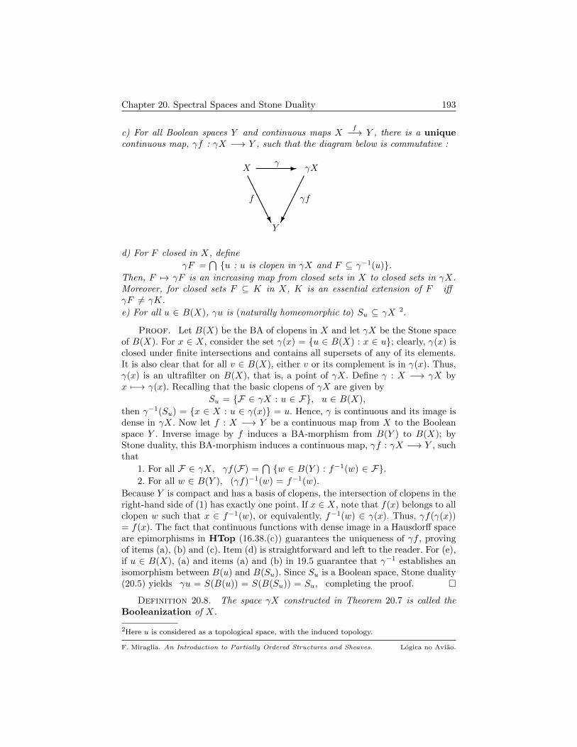
Chapter 20. Spectral Spaces and Stone Duality 193
c) For all Boolean spaces Y and continuous maps Xf−→ Y , there is a unique
continuous map, γf : γX −→ Y , such that the diagram below is commutative :
X - γX
f γf
Y
γ
AAAAAU
d) For F closed in X, define
γF =⋂u : u is clopen in γX and F ⊆ γ−1(u).
Then, F 7→ γF is an increasing map from closed sets in X to closed sets in γX.Moreover, for closed sets F ⊆ K in X, K is an essential extension of F iffγF 6= γK.
e) For all u ∈ B(X), γu is (naturally homeomorphic to) Su ⊆ γX 2.
Proof. Let B(X) be the BA of clopens in X and let γX be the Stone spaceof B(X). For x ∈ X, consider the set γ(x) = u ∈ B(X) : x ∈ u; clearly, γ(x) isclosed under finite intersections and contains all supersets of any of its elements.It is also clear that for all v ∈ B(X), either v or its complement is in γ(x). Thus,γ(x) is an ultrafilter on B(X), that is, a point of γX. Define γ : X −→ γX byx 7−→ γ(x). Recalling that the basic clopens of γX are given by
Su = F ∈ γX : u ∈ F, u ∈ B(X),
then γ−1(Su) = x ∈ X : u ∈ γ(x) = u. Hence, γ is continuous and its image isdense in γX. Now let f : X −→ Y be a continuous map from X to the Booleanspace Y . Inverse image by f induces a BA-morphism from B(Y ) to B(X); byStone duality, this BA-morphism induces a continuous map, γf : γX −→ Y , suchthat
1. For all F ∈ γX, γf(F) =⋂w ∈ B(Y ) : f−1(w) ∈ F.
2. For all w ∈ B(Y ), (γf)−1(w) = f−1(w).
Because Y is compact and has a basis of clopens, the intersection of clopens in theright-hand side of (1) has exactly one point. If x ∈ X, note that f(x) belongs to allclopen w such that x ∈ f−1(w), or equivalently, f−1(w) ∈ γ(x). Thus, γf(γ(x))= f(x). The fact that continuous functions with dense image in a Hausdorff spaceare epimorphisms in HTop (16.38.(c)) guarantees the uniqueness of γf , provingof items (a), (b) and (c). Item (d) is straightforward and left to the reader. For (e),if u ∈ B(X), (a) and items (a) and (b) in 19.5 guarantee that γ−1 establishes anisomorphism between B(u) and B(Su). Since Su is a Boolean space, Stone duality(20.5) yields γu = S(B(u)) = S(B(Su)) = Su, completing the proof.
Definition 20.8. The space γX constructed in Theorem 20.7 is called theBooleanization of X.
2Here u is considered as a topological space, with the induced topology.
F. Miraglia. An Introduction to Partially Ordered Structures and Sheaves. Logica no Aviao.
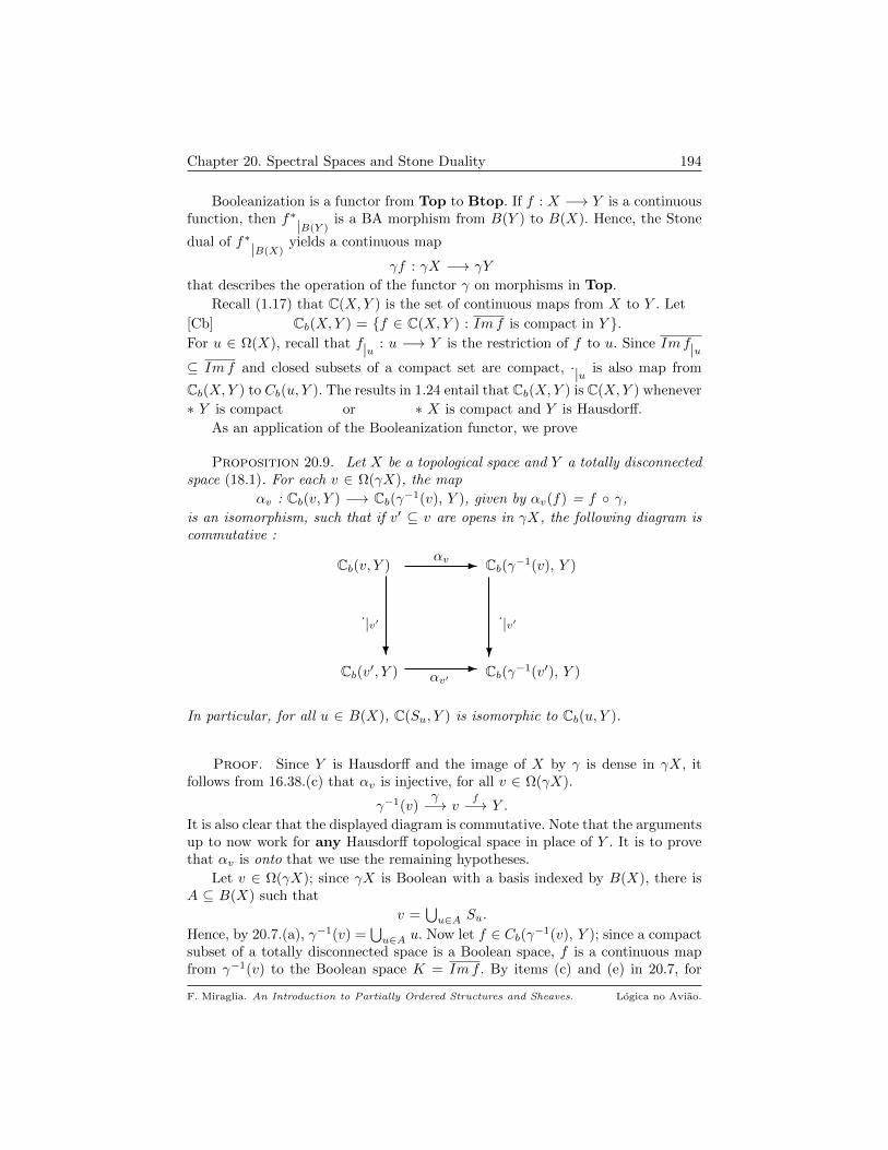
Chapter 20. Spectral Spaces and Stone Duality 194
Booleanization is a functor from Top to Btop. If f : X −→ Y is a continuousfunction, then f∗|B(Y )
is a BA morphism from B(Y ) to B(X). Hence, the Stone
dual of f∗|B(X)yields a continuous map
γf : γX −→ γY
that describes the operation of the functor γ on morphisms in Top.
Recall (1.17) that C(X,Y ) is the set of continuous maps from X to Y . Let
[Cb] Cb(X,Y ) = f ∈ C(X,Y ) : Imf is compact in Y .For u ∈ Ω(X), recall that f|u : u −→ Y is the restriction of f to u. Since Imf|u⊆ Imf and closed subsets of a compact set are compact, ·|u is also map from
Cb(X,Y ) to Cb(u, Y ). The results in 1.24 entail that Cb(X,Y ) is C(X,Y ) whenever
∗ Y is compact or ∗ X is compact and Y is Hausdorff.
As an application of the Booleanization functor, we prove
Proposition 20.9. Let X be a topological space and Y a totally disconnectedspace (18.1). For each v ∈ Ω(γX), the map
αv : Cb(v, Y ) −→ Cb(γ−1(v), Y ), given by αv(f) = f γ,
is an isomorphism, such that if v′ ⊆ v are opens in γX, the following diagram iscommutative :
Cb(v′, Y )
Cb(v, Y )
?
- Cb(γ−1(v), Y )
·|v′
αv
Cb(γ−1(v′), Y )
·|v′
αv′
?-
In particular, for all u ∈ B(X), C(Su, Y ) is isomorphic to Cb(u, Y ).
Proof. Since Y is Hausdorff and the image of X by γ is dense in γX, itfollows from 16.38.(c) that αv is injective, for all v ∈ Ω(γX).
γ−1(v)γ−→ v
f−→ Y .
It is also clear that the displayed diagram is commutative. Note that the argumentsup to now work for any Hausdorff topological space in place of Y . It is to provethat αv is onto that we use the remaining hypotheses.
Let v ∈ Ω(γX); since γX is Boolean with a basis indexed by B(X), there isA ⊆ B(X) such that
v =⋃u∈A Su.
Hence, by 20.7.(a), γ−1(v) =⋃u∈A u. Now let f ∈ Cb(γ−1(v), Y ); since a compact
subset of a totally disconnected space is a Boolean space, f is a continuous mapfrom γ−1(v) to the Boolean space K = Imf . By items (c) and (e) in 20.7, for
F. Miraglia. An Introduction to Partially Ordered Structures and Sheaves. Logica no Aviao.
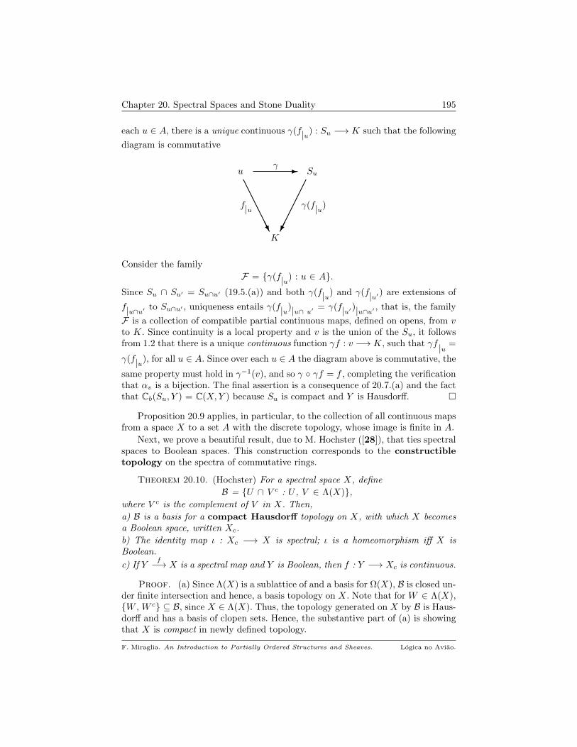
Chapter 20. Spectral Spaces and Stone Duality 195
each u ∈ A, there is a unique continuous γ(f|u) : Su −→ K such that the following
diagram is commutative
u - Su
f|u γ(f|u)
K
γ
AAAAAAU
Consider the family
F = γ(f|u) : u ∈ A.Since Su ∩ Su′ = Su∩u′ (19.5.(a)) and both γ(f|u) and γ(f|u′) are extensions of
f|u∩u′ to Su∩u′ , uniqueness entails γ(f|u)|u∩ u′= γ(f|u′)|u∩u′ , that is, the family
F is a collection of compatible partial continuous maps, defined on opens, from vto K. Since continuity is a local property and v is the union of the Su, it followsfrom 1.2 that there is a unique continuous function γf : v −→ K, such that γf |u =
γ(f|u), for all u ∈ A. Since over each u ∈ A the diagram above is commutative, the
same property must hold in γ−1(v), and so γ γf = f , completing the verificationthat αv is a bijection. The final assertion is a consequence of 20.7.(a) and the factthat Cb(Su, Y ) = C(X,Y ) because Su is compact and Y is Hausdorff.
Proposition 20.9 applies, in particular, to the collection of all continuous mapsfrom a space X to a set A with the discrete topology, whose image is finite in A.
Next, we prove a beautiful result, due to M. Hochster ([28]), that ties spectralspaces to Boolean spaces. This construction corresponds to the constructibletopology on the spectra of commutative rings.
Theorem 20.10. (Hochster) For a spectral space X, define
B = U ∩ V c : U , V ∈ Λ(X),where V c is the complement of V in X. Then,
a) B is a basis for a compact Hausdorff topology on X, with which X becomesa Boolean space, written Xc.
b) The identity map ι : Xc −→ X is spectral; ι is a homeomorphism iff X isBoolean.
c) If Yf−→ X is a spectral map and Y is Boolean, then f : Y −→ Xc is continuous.
Proof. (a) Since Λ(X) is a sublattice of and a basis for Ω(X), B is closed un-der finite intersection and hence, a basis topology on X. Note that for W ∈ Λ(X),W , W c ⊆ B, since X ∈ Λ(X). Thus, the topology generated on X by B is Haus-dorff and has a basis of clopen sets. Hence, the substantive part of (a) is showingthat X is compact in newly defined topology.
F. Miraglia. An Introduction to Partially Ordered Structures and Sheaves. Logica no Aviao.

Chapter 20. Spectral Spaces and Stone Duality 196
In any topological space, compact sets are closed under finite unions. Further-more, the intersection of a compact set and a closed set is compact (1.24.(b)).Hence, all elements of B as well as their complements, are compact in the originaltopology on X. Further, since finite intersections of complements of elements inB can be expressed as finite unions of members of B, we get the following simple,but crucial
Fact 1. All finite intersections of sets of the form U ∪ V c, U, V in Λ(X), arecompact in (the original topology of) X.
The reader should remark the importance in all this of Λ(X) being closedunder finite intersections. Now, since B is a basis for the topology on Xc, everyclosed set in Xc is the intersection of a collection of closed sets (in Xc) of theform U ∪ V c, with U, V ∈ Λ(X). Thus, to show that Xc is compact, it enough toverify that if A is a collection of sets of the form U ∪ V c, with U and V compactopens in X, possessing the finite intersection property, then
⋂A 6= ∅. Such a set
A will remain fixed throughout the remaining part of the argument. By Fact 1,the intersection of all finite subsets of A is compact in the original topology of X.
Define
T = F ⊆ X : F is closed in X and F ∩⋂B 6= ∅, for all B ⊆f A,
partially ordered by inclusion. Clearly, T is not empty since X ∈ T . Let C be achain in T . We show that the closed set
⋂C is in T . To see this, fix W =
⋂B,
B ⊆f A. For F ∈ C, F ∩ W is a non-empty closed set in W , and so, since C is achain, the family
F ∩ W : F ∈ Chas the fip. The compactness of W implies that
⋂C ∩ W 6= ∅. By Zorn’s Lemma
(2.20), there is K minimal in T ; K is closed in X and K ∩ W 6= ∅, for all W ∈ A.
Fact 2. K is irreducible in X.
Proof. Suppose K = F ∪ G, with F and G closed in X. If for some B ⊆f A, wehad G ∩
⋂B = ∅, then, it follows that for all finite subsets B′ ⊆ A, we must have
F ∩⋂B′ 6= ∅. Since K is minimal with this property, it follows that K = F . The
argument just presented is symmetric in F and G, proving that K is irreducible.
Since X is spectral, K has a generic point p, K = p. The proof of (a) willbe finished as soon as we show that p ∈ W , for all W ∈ A. Observe that for openU in X,
K ∩ U 6= ∅ iff p ∈ U .
Let U ∪ V c ∈ A; if p 6∈ U , then K ∩ U = ∅, because U is open. ConsiderF = K ∩ V c; F is closed and non-empty, because K ∈ T . If B is a finite subsetof A, set W =
⋂B; then W ∩ (U ∪ V c) is the intersection of a finite subset of A
and so, since K is in T and K ∩ U = ∅, we must have
K ∩ W ∩ V c = F ∩ W 6= ∅.Since B is an arbitrary finite subset of A, we conclude that F ∈ T . From F ⊆ Kand the minimality of K in T , it follows that F = K, and p ∈ V c, verifying (a).
Part (b) is immediate from the construction. As for (c), if the map f fromY to X is spectral, then for all U ∈ Λ(X), f−1(U) is compact open in Y , i.e.,
F. Miraglia. An Introduction to Partially Ordered Structures and Sheaves. Logica no Aviao.
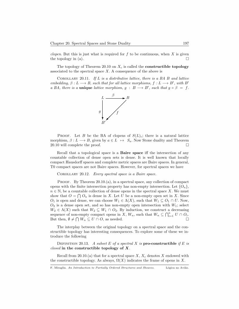
Chapter 20. Spectral Spaces and Stone Duality 197
clopen. But this is just what is required for f to be continuous, when X is giventhe topology in (a).
The topology of Theorem 20.10 on Xc is called the constructible topologyassociated to the spectral space X. A consequence of the above is
Corollary 20.11. If L is a distributive lattice, there is a BA B and latticeembedding, β : L −→ B, such that for all lattice morphisms, f : L −→ B′, with B′
a BA, there is a unique lattice morphism, g : B −→ B′, such that g β = f .
B′
L
?
- B
g
β
f
Proof. Let B be the BA of clopens of S(L)c; there is a natural latticemorphism, β : L −→ B, given by a ∈ L 7→ Sa. Now Stone duality and Theorem20.10 will complete the proof.
Recall that a topological space is a Baire space iff the intersection of anycountable collection of dense open sets is dense. It is well known that locallycompact Hausdorff spaces and complete metric spaces are Baire spaces. In general,T0 compact spaces are not Baire spaces. However, for spectral spaces we have
Corollary 20.12. Every spectral space is a Baire space.
Proof. By Theorem 20.10.(a), in a spectral space, any collection of compactopens with the finite intersection property has non-empty intersection. Let On,n ∈ N, be a countable collection of dense opens in the spectral space X. We mustshow that O =
⋂On is dense in X. Let U be a non-empty open set in X. Since
O1 is open and dense, we can choose W1 ∈ Λ(X), such that W1 ⊆ O1 ∩ U . Now,O2 is a dense open set, and so has non-empty open intersection with W1; selectW2 ∈ Λ(X) such that W2 ⊆ W1 ∩ O2. By induction, we construct a decreasingsequence of non-empty compact opens in X, Wn, such that Wn ⊆
⋂ni=1 U ∩ Oi.
But then, ∅ 6=⋂Wn ⊆ U ∩ O, as needed.
The interplay between the original topology on a spectral space and the con-structible topology has interesting consequences. To explore some of these we in-troduce the following
Definition 20.13. A subset E of a spectral X is pro-constructible if E isclosed in the constructible topology of X.
Recall from 20.10.(a) that for a spectral space X, Xc denotes X endowed withthe constructible topology. As always, Ω(X) indicates the frame of opens in X.
F. Miraglia. An Introduction to Partially Ordered Structures and Sheaves. Logica no Aviao.
Chapter 20. Spectral Spaces and Stone Duality 198
Remark 20.14. Let X be a spectral space.
a) Since the constructible topology in X is finer than its spectral topology, everyclosed set in the original spectral topology is pro-constructible.
b) Because Xc is a Boolean space, with a basis of clopens given by the set B in20.10.(a), if E ⊆ X, the following are equivalent :
(1) E is pro-constructible;
(2) E is an intersection of clopens in Xc;
(3) E is a compact subset of Xc3;
(3) There are compact opens in X, Ui : i ∈ I, Vi : i ∈ I, suchthat E =
⋂i∈I Ui ∪ V ci .
c) It is clear that the finite intersection of pro-constructible subsets of X ispro-constructible. Moreover, if E is pro-constructible and F ⊆ E is closed inXc, then F is pro-constructible. In particular, it follows from (a) that subsetsof pro-constructible sets, that are closed in the spectral topology, are also pro-constructible. 2
Proposition 20.15. Let X be a spectral space.
a) If E 6= ∅ is a pro-constructible subset of X, which is irreducible in the spectraltopology 4, then E has a (unique) generic point.
b) If K is a pro-constructible subset of X, then, with the topology induced by X, Kis a spectral space. Moreover, the constructible topology associated to the spectralspace K is that induced by Xc on K.
Proof. Let Λ(X) be a basis of compact opens in X, that is a sublattice ofΩ(X).
a) Let E be the closure of E in the spectral topology of X. By Lemma 12.10.(b), Eis irreducible in X and so there is p ∈ E such that p is generic for E. We contendthat p ∈ E, which will complete the proof of (a). Assume otherwise; since E isclosed in Xc and
B = U ∩ V c : U , V ∈ Λ(X)is a basis of clopens for the topology in Xc, there are U , V ∈ Λ(X) such that
p ∈ U ∩ V c and U ∩ V c ∩ E = ∅. (I)
Because p ∈ V c, a closed set in X, we get that E ⊆ p = E ⊆ V c. Hence, theequality in (I) yields
∅ = U ∩ V c ∩ E = U ∩ E,
that is impossible because U is an open neighborhood of p ∈ E. The uniquenessof p follows immediately from Lemma 12.10.(c).
b) It is clear that, with the topology induced by X, K is a T0 space, as well asthat
Λ(X)|K =def U ∩ K : U ∈ Λ(X)
3And consequently also in X.4This is a subtle, but important point; since Xc is Boolean, its only non-empty irreducible subsetsare its points.
F. Miraglia. An Introduction to Partially Ordered Structures and Sheaves. Logica no Aviao.

Chapter 20. Spectral Spaces and Stone Duality 199
is a basis and a sublattice of Ω(K) = W ∩ K : W ∈ Ω(X). We must show thatfor all U ∈ Λ(X), U ∩ K is compact in K. Since K is closed in Xc, U is clopen inXc and this last space is compact, it follows that U ∩K is compact in Xc. Now, thefact that the constructible topology is finer than the spectral topology guaranteesthat U ∩ K, with the topology induced by X, is also compact. In particular, Kitself is a compact space.
It remains to check that if E is a non-empty irreducible closed set in K, thenE has a generic point. By Remark 20.14.(c), we know that E is pro-constructibleand so the desired conclusion follows immediately from (a). It is straightforwardthat the constructible topology associated to the topology induced by X on K isthat induced by Xc on K, ending the proof.
As an application, we prove that certain limits of spectral spaces − in par-ticular, products and projective limits − are spectral, and also determine theconstructible topology on these limits. We start with
Theorem 20.16. If Xi, i ∈ I, is a family of spectral spaces, then X =∏i∈I Xi,
with the product topology, is a spectral space. Moreover,
Xc =∏i∈I Xic,
that is, the constructible topology on X is the product of the constructible topologieson each coordinate.
Proof. Since each Xi is a compact space, it follows from Tychonoff’s The-orem 1.28 that X =
∏i∈I Xi, with the product topology, is a compact space; it
is straightforward that X is T0; if Λ(Xi) is the family of compact opens in Xi,i ∈ I, Exercise 1.32 guarantees that, with L(α) =
∏i∈α Λ(Xi),
L = p(U) : U ∈ L(α) and α ∈ Fin(I), (*)
is a basis of compact opens for the product topology on X and a sublattice ofΩ(X).
Let X =∏i∈I Xic be the product of the Boolean spaces that arise when the
Xi are endowed with the constructible topology. Again by Tychonoff’s Theorem,X is compact and, in fact, a Boolean space, because by Exercise 1.32, the set
B = p(V ) : v ∈ B(α) and α ∈ Fin(I), (**)
where B(α) =∏i∈α Bi
5, is a basis for the product topology on X, consisting of
clopen sets 6. Set
γ : X −→ X, given by γ(ξ) = ξ; (***)
since the topology on X is finer than that in X (because this is true for eachcoordinate), γ is a continuous map.
For i ∈ I, we shall write πi both for the projection of X onto Xi and for theprojection of X onto Xic.
5Bi = U ∩ V c : U , V ∈ Λ(Xi), as in Theorem 20.10.6As sets, we have X = X; but it seemed advisable to give distinct names to distinct topologicalspaces.
F. Miraglia. An Introduction to Partially Ordered Structures and Sheaves. Logica no Aviao.
Chapter 20. Spectral Spaces and Stone Duality 200
Since X is compact, T0 and has a basis of compact opens that is a sublattice ofΩ(X), to show that it is spectral we must prove that every non-empty irreducibleclosed set in X has a generic point. This is a consequence of the following:
Fact 20.17. Let E be a non-empty irreducible subset of X and let u ∈ X.For each i ∈ I, let ui = πi(u) and Ei = πi(E)
a) u ∈ E ⇔ ∀ i ∈ I, ui ∈ Ei.b) If E is closed in X, then ∀ i ∈ I, Ei is an irreducible pro-constructible subsetof Xi.
Proof. a) The implication (⇒) is immediate from the continuity of each πi.For the converse, assume, to obtain a contradiction, that u 6∈ E; then, there is afinite subset α of I and for each j ∈ α an open set Uj ⊆ XJ , so that the openU =
∏j∈α Uj ×
∏i∈I\α Xi is a neighborhood of u, disjoint from E. For j ∈ α, let
Vj = Uj ×∏i 6=j Xi; then, U =
⋂j∈α Vj and so E ⊆
⋃j∈α V
cj , a union of closed
sets in X. Since E is irreducible, for some k ∈ α we have E ⊆ V ck , i.e., E ∩ Vk = ∅;since u ∈ Vk, this contradicts the assumption u ∈ E, establishing (a).
b) Since the topology on X is finer than that of X, E is closed, and so compactin X. The continuity of πi : X −→ Xic entails that πi(E) is compact in Xic. SinceXic is Hausdorff, πi(E) is closed in Xic and thus pro-constructible in Xi. Withrespect to irreducibility, suppose that F1, F2 are closed sets in Xi such that
πi(E) ⊆ F1 ∪ F2.
Then, E ⊆ π−1i (F1) ∪ π−1
i (F2); since E is irreducible in X, we conclude that
E ⊆ π−1i (F1) or E ⊆ π−1
i (F2). (****)
Hence, (****) and the surjectivity of πi entails
πi(E) ⊆ πi(π−1i (F1)) = F1 or πi(E) ⊆ πi(π
−1i (F2)) = F2,
and πi(E) is irreducible in X, completing the proof of the Fact.
Now let F be a non-empty irreducible closed in X. Fact 20.17.(b) and Propo-sition 20.15.(a) yield, for each i ∈ I, a generic point, xi ∈ πi(F ). Let x ∈ X be the
point whose coordinates are the xi ∈ πi(F ), i ∈ I. Recalling that πi(F ) = xi,it follows readily from item (a) in Fact 20.17 that x belongs to F and is a genericpoint for F , establishing the spectrality of X.
To finish the proof we need to verify that X is homeomorphic to Xc. In viewof item (c) of Theorem 20.10 and the fact that a continuous bijection betweencompact Hausdorff spaces is a homeomorphism, it suffices to check that the con-tinuous map γ in (***) above is spectral, which in turn reduces to verifying thatif p(U) ∈ L, then γ−1(p(U)) is compact in X. But this is clear, since γ−1(p(U)) =p(U) ∈ B (as in (**)), in fact a clopen set in X, ending the proof.
Theorem 20.16 and Proposition 20.15 yield
Theorem 20.18. Let 〈 I,≤〉 be a poset and let D : I −→ Spec be an I-diagram of spectral spaces, that is, a family Xi : i ∈ I of spectral spaces andspectral maps, fij : Xi −→ Xj (i ≤ j in I), satisfying for all i ≤ j ≤ k in I
F. Miraglia. An Introduction to Partially Ordered Structures and Sheaves. Logica no Aviao.

Chapter 20. Spectral Spaces and Stone Duality 201
(1) fii = IdXi ;
(2) fik = fjk fij.
Xi- Xj
fik fjk
Xk
fij
AAAAAU
Then, T = lim← D exists in Spec and the constructible topology on T is the limit
of the I-diagram whose vertices are the Xic and whose arrows are the fij (i ≤ j).
Proof. The proof will show that in fact the limit of D, in the category oftopological spaces, is spectral and hence the limit of D in Spec.
Let X =∏i∈I Xi; by 20.16, X is spectral and that Xc =
∏i∈I Xic. Recalling
Corollary 17.12, let
T = z ∈ X : ∀ i ≤ j in I, fij(πi(z)) = πj(z), (I)
endowed with the topology induced by X =∏i∈I Xi. We now prove
Fact 20.19. T is pro-constructible in X.
Proof. It must be verified that T is closed in Xc. Let x = (xi)i∈I be a point inXc, outside T . Hence, for some i ≤ j in I, we have that
xj = πj(xj) 6= fij(xi) = fij(πi(x)).
Since Xjc is a Hausdorff space, there are disjoint clopens in Xjc, Vj , V′j , such that
xj ∈ Vj and fij(xi) ∈ V ′j . The continuity of fij guarantees that Vi = f−1ij (V ′j ) is
a clopen set in Xic. Let α = i, j and consider, with notation as in (**) in theproof of 20.16, the clopen p(U) ∈ B, where U = 〈Vi, Vj 〉. Then, p(U) is a clopenneighborhood of x in Xc, that is disjoint from T . Indeed, clearly x ∈ p(U); if y =(yi)i∈I ∈ p(U), then yi ∈ Vi, while yj ∈ Vj . Hence, fij(yi) ∈ V ′j , which is disjointfrom Vj ; in particular, fij(yi) 6= yj , showing that y 6∈ T . The above reasoning hasshown that T c is open in Xc, as needed to establish Fact 20.19.
It follows immediately from Proposition 20.15 that T , with the topology in-duced by X, is a spectral space. Moreover, the same result guarantees that Tc isthe space resulting from endowing T with the topology of Xc.
Consider the systems T = 〈T ; πi|T : T −→ Xi; 〉
T c = 〈Tc; πi|Tc : Tc −→ Xic. 〉
The proof will be completed as soon as it is verified that
T = lim← D and T c = lim← Dc, (II)
where Dc is the I-diagram having as vertices the Xic and as arrows the fij . Weshall prove the first equality in (II); the proof of the second is analogous and leftto the reader. The first step is to show that T is a cone over D, that is, for i ≤ jin I, the diagram below left is commutative :
F. Miraglia. An Introduction to Partially Ordered Structures and Sheaves. Logica no Aviao.

Chapter 20. Spectral Spaces and Stone Duality 202
T - Xi
πj |T fij
Xj
πi|T
AAAAAU
Y - Xi
gj(Y) fij
Xj
gi
AAAAAU
For x = (xi)i∈I ∈ T , we have, by the definition of T in (I),
fij(πi(x)) = πj(x) = xj ,
and the diagram above left is indeed commutative. Next, let
Y = 〈Y ; gi : Y −→ Xi 〉be a cone over D in Spec, i.e., Y is a spectral space, the gi are spectral mapsand for all i ≤ j in I, diagram (Y) above right is commutative. For y ∈ Y , definef : Y −→ T by
f(y)(i) = gi(y),
that is, f(y) is the I-sequence whose ith-coordinate is gi(y). To check that f(y) isindeed in T , assume that i ≤ j in I. Then, Y being a cone over D, the commuta-tivity of diagram (Y) above yields
fij(f(y)(i)) = fij(gi(y)) = gj(y) = f(y)(j),
as needed. The uniqueness of f is straightforward. It remains to show that f isspectral, which reduces to verifying that if p(U) ∈ L (as in (*) in the proof of20.16), then f−1(p(U)) is a compact open in Y . Let α ∈ Fin(I) be such that U= 〈Ui 〉i∈α; then, it is easily established that
f−1(p(U)) =⋂i∈α g
−1i (Ui),
a compact open in Y because it is spectral and each gi is a spectral map. Hence,the cone T is lim← D, ending the proof.
Remark 20.20. a) If fact, Theorem 20.16 is a consequence of Theorem 20.18,for the former corresponds to the case in which the poset I is discrete, i.e., i ≤ jiff i = j. However, it seemed that the exposition would become clearer if 20.16,that is interesting in its own right, was proven first.
For a rather comprehensive information on the category of spectral spaces, thereader is referred to Theorem 7 and 8, as well as Propositions 9 and 10 in [28].
b) As a special case of Theorem 20.18, we obtain that a projective limit of spectralspaces is spectral, as well as that the constructible topology on the projective limitis the projective limit of the corresponding constructible topologies.
c) If I = ∅, then Theorems 20.16 and 20.18 correspond to the empty product,yielding
lim← D = ∗,
F. Miraglia. An Introduction to Partially Ordered Structures and Sheaves. Logica no Aviao.

Chapter 20. Spectral Spaces and Stone Duality 203
i.e., a singleton, endowed with the only possible topology it can have. Clearly, sucha space is spectral and its constructible and spectral topologies coincide since ∗is a Boolean space. 2
Exercises
20.21. Prove that a topological space T is Boolean iff it is spectral andHausdorff. 2
20.22. Show that the construction in Theorem 20.10 originates a functor fromSpec to BTop, and study its properties. 2
20.23. Let L = [0, 1] be the unit real interval considered as a complete chain.Determine S(L) and the constructible topology on S(L).
Hint : S(L) is the disjoint union ((0, 1] × 0) ∪ ([0, 1) × 1) 2
20.24. Using Stone duality, show that the category Spec, of spectral spacesand maps, is a complete and cocomplete category 7. 2
7Freyd’s Theorem 16.31 may be useful. A nice proof would generalize Theorem 20.18 and theanalogous result for colimits of I-diagrams in Spec.
F. Miraglia. An Introduction to Partially Ordered Structures and Sheaves. Logica no Aviao.
CHAPTER 21
Projective Compact Hausdorff Spaces
The first section of this Chapter discusses extremally disconnected spaces,while in the second it will be shown that the category of compact Hausdorff spaceshas enough projectives.
1. Extremally Disconnected Spaces
We now turn to the discussion of the effect of completeness of a lattice or of aBA on the topological properties of their Stone spaces.
Definition 21.1. A topological space X is
a) completely spectral (cs) iff it is spectral and the interior of the intersectionof any family of compact open sets is compact open.
b) extremally disconnected (ed) iff it is Hausdorff and the closure of everyopen set is clopen.
From 19.7.(e) and Stone duality (20.5) we obtain
Proposition 21.2. Let L be a distributive lattice.
a) L is complete iff S(L) is a completely spectral space. Stone duality establishesa natural bijective correspondence between complete distributive lattices and com-pletely spectral spaces.
b) L is a complete Boolean algebra iff S(L) is a compact extremally disconnectedspace. Stone duality establishes a natural and bijective correspondence betweencomplete Boolean algebras and compact extremally disconnected spaces. 2
If B is a Boolean algebra, there is a natural lattice morphism from B to thecBa of regular opens in S(B) :
a ∈ B 7→ Sa ∈ B(S(B)) ⊆ Reg(S(B)).
Note that the operation of join in Reg(S(B)) involves taking the closure of a union,but for a finite number of clopens this is just their set theoretic union. Thus, theabove map is in fact a lattice morphism. Further, it is injective and by Proposition19.7.(d) it is a regular embedding. Since the family Sa : a ∈ B is a basis forthe topology on S(B), we can generalize 18.13, with the help of 14.6 :
Proposition 21.3. If B is a BA, then Reg(S(B)) is the completion of B.
If X is a set then 2X is a cBa and so its Stone space, S(2X), is a compactextremally disconnected space, written βX.
204
Chapter 21. Projective Compact Hausdorff Spaces 205
Remark 21.4. By Exercise 21.21, it is possible to map X into βX in a naturalway :
(β) x ∈ X 7−→ x→ = A ⊆ X : x ∈ A ∈ βX.
If X is given the discrete topology (all points are open), then the above map isa homeomorphism of X onto its image, for all principal ultrafilters in βX areisolated points. Further, if SA is a non-empty clopen set in βX, then A is a non-empty subset of X and so, any of its points will determine a principal ultrafilterin SA. This means that the image of map defined in (β) is a dense open set inβX. Thus, the Stone space construction has given us a compactification of thediscrete space X. To develop the topological and functional analytic properties ofthis construction, we need to recall the relation between filters and convergence ina topological space. 2
Recall (§ after 2.26) that a subset S of a lattice L is a (proper) filter basisif S 6= ∅, ⊥ 6∈ S and
∗ S is down directed, that is, for a, b ∈ S, ∃ c ∈ S such that c ≤ a ∧ b.
Definition 21.5. Let X, Y be topological spaces and let F ⊆ 2X be a filter
basis. Let x ∈ X, y ∈ Y and let Xf−→ Y be a map.
a) x is an accumulation point of F iff x ∈⋂A∈F A. 1
b) F converges to x (F −→ x or lim F = x) iff νx is contained in the filtergenerated by F .
c) f converges to y along F (limF f = y) iff f(F ) = f(A) : A ∈ F is afilter basis in Y , which converges to y.
Exercise 21.22 registers some of the fundamental properties of these concepts.Now we prove
Proposition 21.6. Let X be a set, βX be the Stone space of 2X and letβ : X −→ βX be the map in 21.4.(β). If Y is a compact space and f : X −→ Yis a continuous map, then f has a unique continuous extension to βX, that is,there is g : βX −→ Y , such that g β = f .
Proof. We begin with
Fact. Let F be an ultrafilter on 2X . Then, f(F ) = f(A) : A ∈ F is a convergentfilter base, to a unique point in the closure of f(X). Further, if F = x→ isprincipal, then f(F ) converges to fx.
Proof. Since F is a proper filter and f(A ∩ B) ⊆ f(A) ∩ f(B), f(F ) is a filterbase in Y . By compactness (21.22.(d)), this filter base has an accumulation point,
y ∈⋂A∈F f(A). Clearly, y ∈ f(X).
To prove that f(F ) −→ y, let V be an open neighborhood of y in Y ; since
V ∩⋂A∈F f(A) 6= ∅, it follows that for A ∈ F , f−1(V ) ∩ A is non-empty. Thus,
f−1(V ) ∪ F has the fip, and the maximality of F yields f−1(V ) ∈ F . Since
1A is the closure of A.
F. Miraglia. An Introduction to Partially Ordered Structures and Sheaves. Logica no Aviao.
Chapter 21. Projective Compact Hausdorff Spaces 206
f(f−1(V )) ⊆ V , we conclude that V is in the filter generated by f(F ), as needed.Because Y is Hausdorff, a filter base can have only one limit (21.22.(c)).
If F is principal, F = x→, then fx is an accumulation point of f(F ). The proofgiven above shows that f(F ) converges to any its accumulation points. Hence,f(x→) −→ fx, completing the proof of the Fact.
Define g : βX −→ Y by g(F ) = limF f ; by the Fact, g is a function and anextension of f . It remains to prove that it is continuous. Let V be an open setin Y ; to show that g−1(V ) is open in βX, let F be such that g(F ) ∈ V . Sincecompact spaces are regular, choose W ∈ νg(F ), such that W ⊆ V and let A =
g−1(W ). Exactly as above, we can show that A ∪ F has the fip, and so A ∈ F ,that is, F ∈ SA. If G ∈ SA then the construction of g yields
g(G) ∈ f(A) ⊆ W ⊆ V .
Thus, F ∈ SA ⊆ g−1(V ), as needed. Uniqueness is immediate, because X is densein βX and Y is Hausdorff.
Proposition 21.6 shows that βX is the Stone-Cech compactification of thediscrete space X, since the defining properties of the Stone-Cech compactificationof X are : X is densely embedded in a compact space Y such that every continuousfunction from X to any compact space can be extended to Y . Clearly, this propertydetermines the space Y , whenever it exists, up to homeomorphism. By Exercise16.44, every completely regular space has a Stone-Cech compactification. However,the method described here to obtain it is quite distinct from the one in 16.44.
Recall (1.16(a)) that the density, d(X), of a space X is the least cardinal suchthat X it has a dense subset of that cardinality. Clearly, X always has a densesubset of cardinality d(X). Note that if I is a set, then, d(βI) = card(I). Hence,βN is separable, i.e., d(βN) = ω.
Corollary 21.7. Every compact topological space is the continuous imageof a compact extremally disconnected space of the same density. In particular, allseparable compact spaces are a continuous image of βN.
Proof. Let Y be a dense subset of cardinality d(X), of the compact spaceX. By 21.6, the injection of Y into X has a continuous extension, f : βY −→ X.Since Im f is dense and compact in a Hausdorff space, we conclude that f is ontoX. To finish the proof, just observe that d(βY ) = card(Y ) = d(X).
By 21.7, extremally disconnected compacts are “projective generators” in thecategory of compact spaces. We will discuss this theme in depth in the next section.
We now wish to show that dyadic spaces cannot be extremally disconnected,generalizing Proposition 18.13. Our method will be distinct from that in [13]. Tothis end, we prove (compare 18.20)
Lemma 21.8. Every infinite cBa contains a copy of 2N.
Proof. Let B be an infinite cBa. We start by constructing a strictly decreas-ing sequence, an, n ≥ 0, of elements of B, such that a←n is infinite, for all n ≥ 0.Set a0 = >; by induction, assume that we have constructed ak, with ak+1 < ak,
F. Miraglia. An Introduction to Partially Ordered Structures and Sheaves. Logica no Aviao.
Chapter 21. Projective Compact Hausdorff Spaces 207
0 ≤ k ≤ (n− 1). Since a←n is infinite, select b < an; because b ∨ (¬ b ∧ an) = an,all c ∈ a←n can be written as a join of elements in b← and (¬ b ∧ an)←. It followsthat either b← or (¬ b ∧ an)← must be infinite. Set
an+1 =
b if b← is infinite
¬ b ∧ an otherwise
For n ≥ 0, let bn = (an ∧ ¬ an+1) = an 4 an+1. Note that the bn are all pairwisedisjoint and distinct from ⊥. Moreover,∨
n≥0 an =∨n≥0 bn = >.
Now define f : 2N −→ B, by
f(S) =∨n∈S bn.
Clearly, f(∅) = ⊥ (=∨∅) and f(N) = >. If S, T ∈ 2N and n ∈ (S − T ), then
bn ≤ f(S), but bn ∧ f(T ) = ⊥, showing that f is injective. Next, the distributivelaw in 8.4 yields, for all S ∈ 2N,
f(S) ∧ f(N − S) =∨k∈S bk ∧
∨j 6∈S bj =
∨(k,j)∈(S×Sc) bk ∧ bj = ⊥,
because the bn are pairwise disjoint. Clearly, f(S) ∨ f(N − S) = >, and hence,f(N − S) = ¬ f(S), that is, f preserves complements. To complete the proof, itis enough to show that f preserves meets. Another application of 8.4 yields
f(S) ∧ f(T ) =∨k∈S bk ∧
∨j∈T bj =
∨(k,j)∈S×T bk ∧ bj
=∨n∈S∩T bn = f(S ∩ T ),
completing the proof.
Remark 21.9. The proof of 21.8 applies to σ-algebras, that is BAs with allcountable joins and meets. Hence, any σ-algebra (or cBa) has cardinal larger thanor equal to that of the continuum (2N). 2
A categorical duality establishes a correspondence between dual concepts :monic and epic, injectives and projectives, etc. In the case of Stone duality, anembedding of BAs originates an epic in the category of Boolean spaces, whichby Exercise 16.40 and compactness, are onto continuous maps in BTop. Simi-larly, an epic in BA, which is an onto BA-morphism by 5.17, will give rise to amonic in BTop, that is an injective continuous map. We shall make use of thesecorrespondences in what follows, without further notice.
Corollary 21.10. βN is a continuous image of every extremally disconnectedspace.
Proof. If X is extremally disconnected, then B(X) is a cBa (21.2.(b)). Theinjective BA-morphism, f : 2N −→ B(X), of 21.8, yields, by Stone duality, acontinuous surjection, fS : X −→ βN, as desired.
Proposition 21.11. βN is not a dyadic compact.
Proof. Assume, to get a contradiction, that there is a continuous surjectionπ : 2A −→ βN. For each n ≥ 0, let Vn = π−1(n) be the clopen inverse image ofthe principal ultrafilters n ∈ βN. Clearly,
F. Miraglia. An Introduction to Partially Ordered Structures and Sheaves. Logica no Aviao.
Chapter 21. Projective Compact Hausdorff Spaces 208
(*)
(i) k 6= j ⇒ Vk ∩ Vj = ∅;(ii)
⋃n≥0 Vn is a dense open in 2A,
where the second property follows from the fact that N is dense in βN. By 18.5.(e),for n ≥ 0, there is sn ∈ pFω(A, 2), such that Vn = Vsn . Let K =
⋃n≥0 domsn.
Then K is countable. To keep notation straight, write σn for sn considered as anelement of pFω(K, 2); by Lemma 18.8, we have, for all n ≥ 0,
Vn = Vσn × 2(A−K).
Note that the collection Vσn ; n ≥ 0 satisfies the properties in (*), with K inplace of A. For x ∈ 2K , write x for the element of 2A given, for i ∈ A, by
xi =
xi if i ∈ K1 if i 6∈ K.
Note that if x ∈ Vσn , then x ∈ Vn, n ≥ 0.
Fact 1. Let (xn)n≥0 ⊆ 2K be a sequence such that xn ∈ Vσn , n ≥ 0. Then, thereis an infinite T ⊆ N, such that the sequence xt, t ∈ T , is convergent in 2A.
Proof. Since K is countable, 2K is metric compact. Thus, xn has a convergentsubsequence, xnk −→ x in 2K . Clearly, xnk converges to x. Now, just take T =nk : k ≥ 0; since the xn are all distinct (the Vσn are disjoint), T is an infinitesubset of N.
But we also have
Fact 2. Let T be an infinite subset of N and let T = xt : t ≥ T be a sequence ofelements in 2A, such that xt ∈ Vt, for all t ∈ T . Let Y be a compact space. Then,any map from T to Y can be extended to a continuous map from 2A into Y .
Proof. Let f : T −→ Y be a map; define g : N −→ Y by
g(n) =
f(xn) if n ∈ Tp if n 6∈ T ,
where p is any point in Y . By 21.6, g has a (unique) continuous extension,g : βN −→ Y . But then g π is an extension of f to 2A.
Y
2A
?
- βN
g π
π
g
Let T = xt : t ∈ T be the convergent sequence in Fact 1, with limit x. Since Tis infinite, write T = P ∪ Q, with P , Q infinite and disjoint. Let f : T −→ 0, 1given by
f(xt) =
1 if t ∈ P0 if t ∈ Q.
By Fact 2, f has a continuous extension to 2A. But this is impossible, because thesubsequences of T indexed by P and Q both converge to x.
F. Miraglia. An Introduction to Partially Ordered Structures and Sheaves. Logica no Aviao.
Chapter 21. Projective Compact Hausdorff Spaces 209
We can now prove a strong generalization of 18.13, namely
Theorem 21.12. If X is a dyadic space, then
a) No continuous image of X is extremally disconnected. In particular, X is notextremally disconnected.
b) No infinite Boolean algebra of clopens in X is complete.
Proof. a) Since the class of dyadic spaces is closed under continuous images,it follows from Proposition 21.11 and Corollary 21.10, that no continuous imageof a dyadic space can be extremally disconnected.
b) Let X be a dyadic compact and let B ⊆ B(X) be a complete subalgebra of
clopens in X. Assume, to get a contradiction, that B is infinite. Let Xγ−→ γX
be the Booleanization of X, as in 20.7. Since X is compact and the image of γis dense in γX, it follows that γ is surjective. Moreover, since γX is the Stonespace of B(X), the embedding B −→ B(X) yields, by Stone duality, a continuoussurjection, from γX to S(B). Hence, S(B) is a continuous image of X. But, by21.2, S(B) is extremally disconnected, contradicting (a).
2. Projective Compacts
In this section we discuss projectives in the category of compact Hausdorffspaces and present the construction of the Gleason projective cover of thesespaces.
As already mentioned in section 1, a duality establishes a natural correspon-dence between dual notions, such as epics and monics, injectives and projectives,injective hulls and projective covers. Consequently, Stone duality provides a wayto transfer results about the category BA to the category BTop. For instance,Theorem 20.5, Corollary 15.3, Exercise 15.5 and Corollaries 15.4 and 21.3 yield
Corollary 21.13. A Boolean space is projective in BTop iff it is extremallydisconnected. Every Boolean space X is the continuous image of S(Reg(X)), andthis compact extremally disconnected space is the projective cover of X in BTop.
We go a step further, investigating what happens in the category of compactHausdorff spaces. The properties in Lemma 1.10 will be of constant use.
Proposition 21.14. Let X be a compact (Hausdorff ) space.
a) The following are equivalent:
(1) X is extremally disconnected.
(2) For all open U , V in X, U ∩ V = U ∩ V .
(3) For all open U , V in X, U ∩ V = ∅ implies U ∩ V = ∅.b) If X is a projective compact space, then X is extremally disconnected.
c) X is a projective compact space iff it satisfies :
[split] If Y is a compact space and Yf−→ X is a onto continuous
map, there is a continuous Xg−→ Y , such that f g = IdX .
F. Miraglia. An Introduction to Partially Ordered Structures and Sheaves. Logica no Aviao.
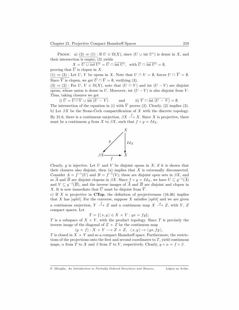
Chapter 21. Projective Compact Hausdorff Spaces 210
Proof. a) (3) ⇒ (1) : If U ∈ Ω(X), since (U ∪ int U c) is dense in X, and
their intersection is empty, (3) yields
X = U ∪ int U c = U ∩ int U c, with U ∩ int U c = ∅,proving that U is clopen in X.
(1) ⇒ (3) : Let U , V be opens in X. Note that U ∩ V = ∅, forces U ∩ V = ∅.Since V is clopen, we get U ∩ V = ∅, verifying (3).
(3) ⇒ (2) : For U , V ∈ Ω(X), note that (U ∩ V ) and int (U − V ) are disjoint
opens, whose union is dense in U . Moreover, int (U − V ) is also disjoint from V .Thus, taking closures we get
i) U = U ∩V ∪ int (U − V ) and ii) V ∩ int (U − V ) = ∅.The intersection of the equation in (i) with V proves (2). Clearly, (2) implies (3).
b) Let βX be the Stone-Cech compactification of X with the discrete topology.
By 21.6, there is a continuous surjection, βXf−→ X. Since X is projective, there
must be a continuous g from X to βX, such that f g = IdX .
βX
X
g
X
IdX
f
?-
Clearly, g is injective. Let U and V be disjoint opens in X; if it is shown thattheir closures also disjoint, then (a) implies that X is extremally disconnected.Consider A = f−1(U) and B = f−1(V); these are disjoint open sets in βX, andso A and B are disjoint clopens in βX. Since f g = IdX , we have U ⊆ g−1(A)and V ⊆ g−1(B), and the inverse images of A and B are disjoint and clopen inX. It is now immediate that U must be disjoint from V .
c) If X is projective in CTop, the definition of projectiveness (16.36) impliesthat X has [split]. For the converse, suppose X satisfies [split] and we are given
a continuous surjection, Yf−→ Z and a continuous map X
g−→ Z, with Y , Zcompact spaces. Let
T = 〈x, y 〉 ∈ X × Y : gx = fy;T is a subspace of X × Y , with the product topology. Since T is precisely theinverse image of the diagonal of Z × Z by the continuous map
(g × f) : X × Y −→ Z × Z, 〈x, y 〉 7→ 〈 gx, fy 〉,T is closed in X × Y and so a compact Hausdorff space. Furthermore, the restric-tions of the projections onto the first and second coordinates to T , yield continuousmaps, α from T to X and β from T to Y , respectively. Clearly, g α = f β.
F. Miraglia. An Introduction to Partially Ordered Structures and Sheaves. Logica no Aviao.
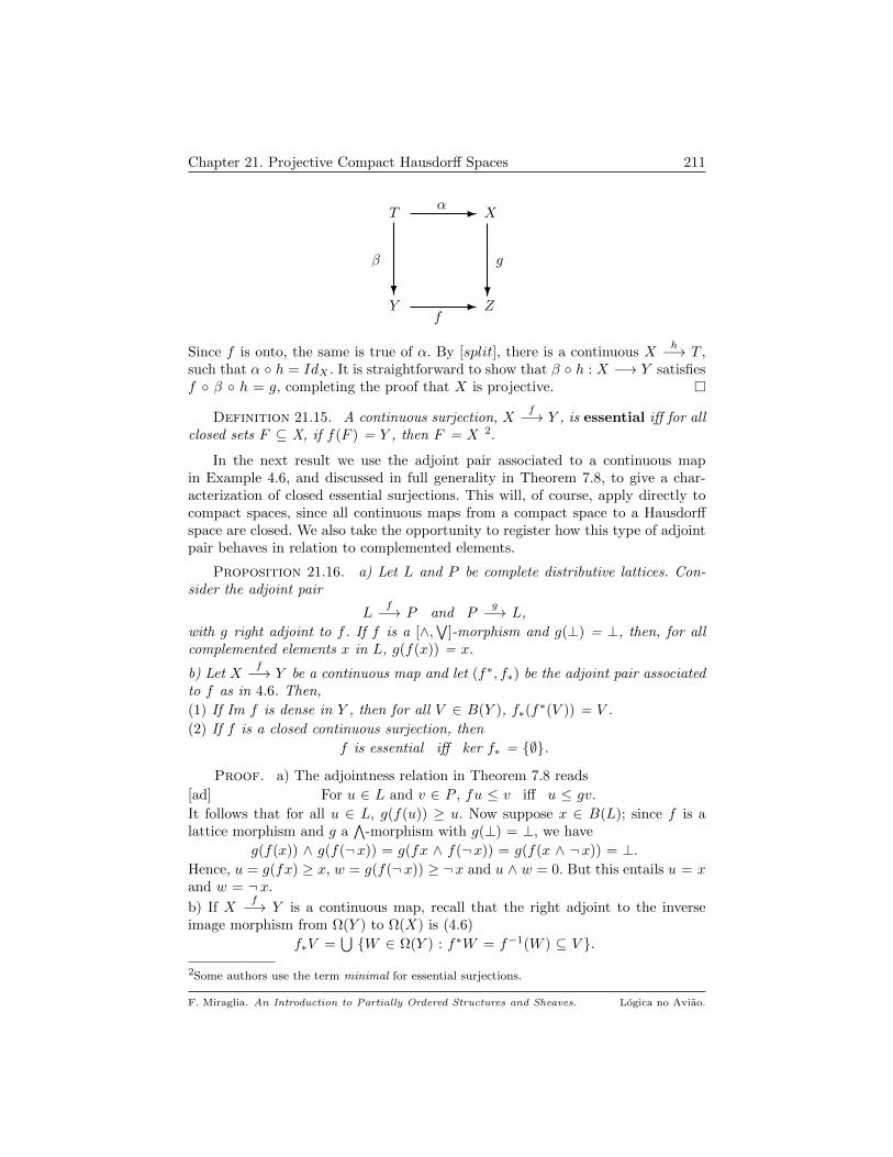
Chapter 21. Projective Compact Hausdorff Spaces 211
Y
T
?
- X
β
α
Z
g
f
?-
Since f is onto, the same is true of α. By [split], there is a continuous Xh−→ T ,
such that α h = IdX . It is straightforward to show that β h : X −→ Y satisfiesf β h = g, completing the proof that X is projective.
Definition 21.15. A continuous surjection, Xf−→ Y , is essential iff for all
closed sets F ⊆ X, if f(F ) = Y , then F = X 2.
In the next result we use the adjoint pair associated to a continuous mapin Example 4.6, and discussed in full generality in Theorem 7.8, to give a char-acterization of closed essential surjections. This will, of course, apply directly tocompact spaces, since all continuous maps from a compact space to a Hausdorffspace are closed. We also take the opportunity to register how this type of adjointpair behaves in relation to complemented elements.
Proposition 21.16. a) Let L and P be complete distributive lattices. Con-sider the adjoint pair
Lf−→ P and P
g−→ L,
with g right adjoint to f . If f is a [∧,∨
]-morphism and g(⊥) = ⊥, then, for allcomplemented elements x in L, g(f(x)) = x.
b) Let Xf−→ Y be a continuous map and let (f∗, f∗) be the adjoint pair associated
to f as in 4.6. Then,
(1) If Im f is dense in Y , then for all V ∈ B(Y ), f∗(f∗(V )) = V .
(2) If f is a closed continuous surjection, then
f is essential iff ker f∗ = ∅.
Proof. a) The adjointness relation in Theorem 7.8 reads
[ad] For u ∈ L and v ∈ P , fu ≤ v iff u ≤ gv.
It follows that for all u ∈ L, g(f(u)) ≥ u. Now suppose x ∈ B(L); since f is alattice morphism and g a
∧-morphism with g(⊥) = ⊥, we have
g(f(x)) ∧ g(f(¬x)) = g(fx ∧ f(¬x)) = g(f(x ∧ ¬x)) = ⊥.
Hence, u = g(fx) ≥ x, w = g(f(¬x)) ≥ ¬x and u ∧ w = 0. But this entails u = xand w = ¬x.
b) If Xf−→ Y is a continuous map, recall that the right adjoint to the inverse
image morphism from Ω(Y ) to Ω(X) is (4.6)
f∗V =⋃W ∈ Ω(Y ) : f∗W = f−1(W ) ⊆ V .
2Some authors use the term minimal for essential surjections.
F. Miraglia. An Introduction to Partially Ordered Structures and Sheaves. Logica no Aviao.

Chapter 21. Projective Compact Hausdorff Spaces 212
Consequently, if the image of f is dense in Y , the only open set in Y whose inverseimage is empty is ∅. The conclusion in (1) now follows from (a). To verify (2),let U be a non-empty open set in X. Because f is essential and closed, there is anon-empty open V in Y , such that V ∩ f(X − U) = ∅. Then,
f∗V ∩ (X − U) ⊆ f∗V ∩ f−1(f(X − U)) = ∅,showing that f∗V ⊆ U . By adjointness, V ⊆ f∗U , and so f∗U 6= ∅, proving thatthe kernel of f∗ = ∅. Conversely, if ker f∗ = ∅, let F be a proper closed subsetof X and U = (X − F ). Since U 6= ∅, we have f∗U 6= ∅. From the adjointnessrelation and f∗U = f∗U , we obtain f∗(f∗U) ⊆ U . But this means that f restrictedto F is not surjective, for there is a non-empty open in Y , whose inverse image isdisjoint from F . Hence, f is essential.
Proposition 21.17. Let Xf−→ Y be a continuous surjection of compact
spaces.
a) There is a compact subspace T of X, such that f|T is an essential surjection
onto Y.
b) If f is essential and Y is extremally disconnected, then f is a homeomorphism.
Proof. a) Define
V = F ⊆ X : F is closed in X and f(F ) = Y ,partially ordered by inclusion. If C is a chain in V, then, for each y ∈ Y , thefamily f−1(y) ∩ F : F ∈ C has the fip. Since f−1(y) is compact, this impliesthat
⋂C ∩ f−1(y) 6= ∅, that is,
⋂C ∈ V. By Zorn’s Lemma (2.20), V has a
minimal element, T . Clearly, f restricted to T is an essential surjection onto Y .
b) Since continuous maps between compact spaces are closed and f is onto Y , toprove that f is a homeomorphism, it is enough to show that it is injective. Let z, tbe distinct points in X and assume, to get a contradiction, that fz = ft = y. Fixdisjoint opens, U ∈ νz and V ∈ νt and let f∗ : Ω(X) −→ Ω(Y ) be the right adjointto the inverse image morphism f∗, as in 21.16.(b). Since U ∩ V = ∅, we havef∗U ∩ f∗V = ∅. Y being extremally disconnected, it follows that f∗U is disjointfrom f∗V . Let S and T be the clopen complements of f∗U and f∗V , respectively,in Y . Clearly, S ∪ T = Y . Consequently, y = fz = ft must be in either S or Tand we can suppose, without loss of generality, that y ∈ T . Consider the open setV ∩ f∗T ; it is non-empty, since it contains t. On the other hand, recalling that Tis complemented in Ω(Y ) and item (b) in 21.16, we get
f∗(V ∩ f∗T ) = f∗V ∩ f∗(f∗T ) = f∗V ∩ T = ∅,that is impossible, because f is essential.
If X is a compact Hausdorff space, let G(X) =def S(Reg(X)) be the Stonespace of the cBa Reg(X). G(X) is the Gleason cover of X; it is extremallydisconnected and its points are the ultrafilters in Reg(X).
If F ∈ G(X), V : V ∈ F is a collection of closed sets in X with the fip. Bycompactness, A =
⋂V ∈F V 6= ∅. Let x ∈ A; since X is regular, for each U ∈ νx,
we can select a regular open W ∈ νx, such that W ⊆ U . Notice that W ∪ F hasthe fip in Reg(X); the maximality of F implies that W ∈ F . We have shown (21.5)
F. Miraglia. An Introduction to Partially Ordered Structures and Sheaves. Logica no Aviao.
Chapter 21. Projective Compact Hausdorff Spaces 213
that the filter generated by F in Ω(X) (or 2X) contains νx, that is, F −→ x. SinceX is Hausdorff, A must consist of a single point. Therefore, we have constructeda map
g : G(X) −→ X,
whose basic properties are described in
Proposition 21.18. With g : G(X) −→ X as above,
a) g is onto X.
b) For all open U ∈ Ω(X),
g∗U = g−1(U) =⋃SV : V ∈ Reg(X) and V ⊆ U.
In particular, g is continuous and g∗U = SU , for all U ∈ Reg(X).
c) g is an essential continuous surjection from G(X) onto X.
d) If G(X)f−→ G(X) is a continuous map such that g f = g, then f = IdG(X).
Proof. a) Let x be a point in X; the collection of regular open neighborhoodsof x is a proper filter in Reg(X) and so can be extended to an ultrafilter F onReg(X). Clearly, the filter generated by F in Ω(X) contains νx, that is gF = x.
b) Let U be open in X and let F be an ultrafilter in Reg(X), such that gF ∈ U .Let V be a regular open neighborhood of gF , such that V ⊆ U . The definition ofg implies that for all G ∈ SV , gG ∈ V ⊆ U . Hence, SV ⊆ g∗U , proving that g∗Uis open and contained in the right side of the equality stated in (b). The reversecontainment is an immediate consequence of the construction of g. The continuityof g is clear. Observe that U is the sup, in the cBa Reg(X), of the collection ofregular V ⊆ U , such that V ⊆ U . By Proposition 19.7.(d),
SU =⋃SV : V ∈ Reg(X) and V ⊆ U = g∗ U .
(c) For U ∈ Reg(X), we have g∗U ⊆ SU ; the adjointness relation [ad] (see proof of21.16 or 7.8) implies that U ⊆ g∗(SU ). Recalling that SU is empty iff U is empty,that the clopens in G(X) are of the form SU , U ∈ Reg(X), and that they form abasis for G(X), we conclude that ker g∗ = ∅. By Proposition 21.16.(b), g is anessential surjection.
(d) Let f : G(X) −→ G(X) be a continuous map, such that g f = g. Sinceg(Im f) = X and g is an essential surjection, it follows that f is onto G(X).Moreover, f must be essential, for if for some proper closed subset, A ⊆ G(X), wehad f(A) = G(X), then g(f(A)) = g(A) = X, contradicting the essential natureof g. But then, the fact that G(X) is extremally disconnected implies that f is ahomeomorphism. Now, for U in Reg(X), (a) entails that g∗U dense in SU . Sincef is a homeomorphism, f∗(g∗U) is dense in the clopen set f∗(SU ). On the otherhand, g f = g yields f∗(g∗U) = g∗U . Thus, f∗(SU ) = SU , for all U ∈ Reg(X).But the only continuous map from G(X) to G(X) that can satisfy this propertyis IdG(X), ending the proof.
We summarize our discussion in
Theorem 21.19. a) A compact Hausdorff space is projective iff it is extremallydisconnected.
F. Miraglia. An Introduction to Partially Ordered Structures and Sheaves. Logica no Aviao.
Chapter 21. Projective Compact Hausdorff Spaces 214
b) For all compact spaces X, the Gleason cover of X, G(X)g−→ X, is the projective
cover of X in the category of compact spaces.
Proof. (a) By items (b) and (c) in Proposition 21.14, it is enough to show
that if X is extremally disconnected, every continuous surjection Yf−→ X has a
section that is, a continuous g : X −→ Y , such that f g is the identity on X.By 21.17.(a), there is a closed subset F of Y , such that h = f|F : F −→ X is an
essential surjection. Since X is extremally disconnected, part (b) of 21.17 impliesthat h is a homeomorphism. The inverse of h provides the desired continuoussection of f .
(b) Let Yf−→ X be a continuous surjection, with Y compact and extremally
disconnected. Since Y is projective, there is a continuous map g : Y −→ G(X),such that g g = f . It remains to show that g is onto. Since G(X) is also projective,there is h : G(X) −→ Y , such that f h = g. From g g = f , we get g (g h)= g, with g h a continuous map from G(X) to G(X). By Proposition 21.14.(d),g h = IdG(X). Hence, g is onto G(X) and the proof is complete.
It is quite clear that the construction of taking the Gleason cover of a compactspace is idempotent, that is, G(G(X) is naturally homeomorphic to G(X).
Exercises
21.20. A compact Hausdorff ed space is Boolean 3. 2
21.21. Recall that an atom in a lattice L is a minimal element 6=⊥ (2.6).
a) A principal filter is maximal iff it is generated by an atom.
b) Let Atm(L) be (possibly empty) set of atoms in L. The map a 7→ a→ definesa bijective correspondence between the atoms of L and the open set of isolatedpoints 4 of S(L). 2
21.22. Let Xf−→ Y be a map, where X and Y are topological spaces. Let F
be a filter basis in X. Then,
a) If F −→ x, then x is an accumulation point of F . If F is a maximal filter inΩ(X) and x is an accumulation point of F , then F −→ x. In particular, if anultrafilter in 2X has an accumulation point, then it converges to that point.
b) f is continuous iff for all x ∈ X and filters F ⊆ 2X , F −→ x ⇒ limF f =f(x).
c) If X is a topological space and x, y ∈ X, the following are equivalent :
(1) X is a Hausdorff space.
(2) For all filter bases F ⊆ 2X , x = lim F = y ⇒ x = y.
(3) For all ultrafilters F ⊆ 2X , x = lim F = y ⇒ x = y.
(4) For all filter bases G on Ω(X), x = lim G = x ⇒ x = y.
3Compact spaces are normal; but even regularity suffices!4A point p is isolated if p is open.
F. Miraglia. An Introduction to Partially Ordered Structures and Sheaves. Logica no Aviao.

Chapter 21. Projective Compact Hausdorff Spaces 215
d) Consider the following conditions :
(1) X is a compact space.
(2) Every filter basis on 2X has an accumulation point.
(3) Every ultrafilter on 2X converges.
(4) Every ultrafilter in Ω(X) converges.
Then, (1) ⇔ (2) ⇔ (3) ⇒ (4). If X is regular (1.20), all four conditions areequivalent.
e) Give an example of a Hausdorff non-compact, non-regular space in which allultrafilters of opens are convergent 5. 2
21.23. Let I be a set and Fi : i ∈ I be a family of fields indexed by I. LetR =
∏i∈I Fi. Then, Spec(R) is homeomorphic to the Stone-Cech compactification
of the discrete space I. 2
21.24. Let CTop be the category of compact Hausdorff spaces and letF : CTop −→ Set be the forgetful functor. What is the relation between βXand F ? 2
5T0, non-Hausdorff examples are easy to find; T2 examples are harder.
F. Miraglia. An Introduction to Partially Ordered Structures and Sheaves. Logica no Aviao.
Part 4
Presheaves over TopologicalSpaces
CHAPTER 22
Geometric Sheaves
In this chapter many proofs are left to the reader. Its contents describe thebasic geometrical object associated to sheaves over topological spaces. Generalreferences for this chapter are [75], [19], [22] and [66]. In [21] the reader willfind an interesting survey of the history of Sheaf Theory and its mathematicalsignificance.
Notation and results of section 1.2 may be used without explicit reference.Recall that Ω(X) is the frame of opens of the topological space X.
Definition 22.1. Let pF (X,E) be the set of partial maps from X to E (2.12).For s, t ∈ pF (X,E), define
[[s = t]] = x ∈ doms ∩ dom t : s(x) = t(x)Let E
p−→ X be a map. A section for p is a map s ∈ pF (X,E) such that
doms ⊆ Imp and p s = Iddoms.
If doms = A ⊆ X, s is a section over A.
If E and X are topological spaces, p is a local homeomorphism iff for alle ∈ E, there is an open U ∈ νe such that p(U) ∈ Ω(X) and p|U : U −→ p(U) is
a homeomorphism 1.
The basic properties of local homeomorphisms and their sections are described in
Proposition 22.2. If Ep−→ X is a local homeomorphism, then
a) p is continuous and open.
b) A section of p over an open subset of X is an open map. If s is a continuoussection of p over u ∈ Ω(X), then s and p|s(u)
are inverse homeomorphisms between
u ∈ Ω(X) and s(u) ∈ Ω(E).
c) p(E) ∈ Ω(X) and Ep−→ p(E) is a local homeomorphism.
d) Let q : F −→ X be a local homeomorphism and f : E −→ F be a map suchthat q f = p. Then, f is continuous iff f is a local homeomorphism.
1νe is the filter of open neighborhoods of e; see the paragraph right after 1.9. Homeomorphismsare defined in 1.17.(d).
217
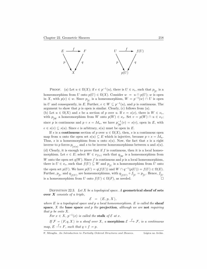
Chapter 22. Geometric Sheaves 218
E - F
p q
X
f
AAAAAU
U - f(U)
p q
p(U)
f
AAAAAU
Proof. (a) Let u ∈ Ω(X); if e ∈ p−1(u), there is U ∈ νe, such that p|U is a
homeomorphism from U onto p(U) ∈ Ω(X). Consider w = u ∩ p(U); w is openin X, with p(e) ∈ w. Since p|U is a homeomorphism, W = p−1(w) ∩ U is open
in U and consequently, in E. Further, e ∈ W ⊆ p−1(u), and p is continuous. Theargument to show that p is open is similar. Clearly, (c) follows from (a).
(b) Let u ∈ Ω(X) and s be a section of p over u. If e = s(x), there is W ∈ νe,with p|W a homeomorphism from W onto p(W ) ∈ νx. Set v = p(W ) ∩ u ∈ νx;
since p is continuous and p s = Idu, we have p−1
|W (v) = s(v), open in E, with
e ∈ s(v) ⊆ s(u). Since e is arbitrary, s(u) must be open in E.
If s is a continuous section of p over u ∈ Ω(X), then, s is a continuous openmap from u onto the open set s(u) ⊆ E which is injective, because p s = Idu.Thus, s is a homeomorphism from u onto s(u). Now, the fact that s is a rightinverse to p forces p|s(u)
and s to be inverse homeomorphisms between u and s(u).
(d) Clearly, it is enough to prove that if f is continuous, then it is a local homeo-morphism. Let e ∈ E; select W ∈ νf(e) such that q|W is a homeomorphism from
W onto the open set q(W ). Since f is continuous and p is a local homeomorphism,there is U ∈ νe, such that f(U) ⊆ W and p|U is a homeomorphism from U onto
the open set p(U). We have p(U) = q(f(U)) and W ∩ q−1(p(U)) = f(U) ∈ Ω(E).Further, p|U and q|f(U)
are homeomorphisms, with q|f(U) f|U = p|U . Hence, f|U
is a homeomorphism from U onto f(U) ∈ Ω(F ), as needed.
Definition 22.3. Let X be a topological space. A geometrical sheaf of setsover X consists of a triple,
E = 〈E, p, X 〉,where E is a topological space and p a local homeomorphism. E is called the sheafspace, X the base space and p the projection, although we are not requiringthat p be onto X.
For x ∈ X, p−1(x) is called the stalk of E at x.
If F = 〈F, q,X 〉 is a sheaf over X, a morphism E f−→ F , is a continuous
map, Ef−→ F , such that q f = p.
F. Miraglia. An Introduction to Partially Ordered Structures and Sheaves. Logica no Aviao.

Chapter 22. Geometric Sheaves 219
E - F
p q
X
f
AAAAAU
Since the (set-theoretical) composition of morphisms is a morphism and the identityis a morphism, we have a category, Shg(X), of geometric sheaves over X.
Example 22.4. If E = 〈E, p,X 〉 is a sheaf over X, the projection p is acontinuous open map. If U is any open set in E, 〈U, p|U , X 〉 is a sheaf over X. In
fact, if S ⊆ X is given the induced topology from X, then 〈 p−1(S), p|p−1(S), S 〉
is a sheaf over S. 2
Example 22.5. Proposition 22.2.(d) implies that if E f−→ F is a morphism ofsheaves, then the triple 〈E, f, F 〉 is a sheaf over F , where E and F are the sheafspaces of E and F , respectively. 2
Definition 22.6. Let E = 〈E, p,X 〉 be a sheaf and let S, T be subsets of X.
a) Write E(S) for the set of continuous sections of p with domain S :
E(S) = S s−→ E : s is a continuous section of pUnless explicit mention to the contrary, it is assumed that S has the topologyinduced by X. Note that E(∅) has precisely one element, written ∗, correspondingto the unique section of E over the empty set.
For x ∈ X, Ex =def E(x) = p−1(x) is the stalk of E at x.
b) If S ⊆ T , define the restriction map
ρTS : E(T ) −→ E(S), given by t 7−→ t|S.
When S = x, write ρTx for ρTx. Note that if S ⊆ T ⊆ K, then
ρKS = ρTS ρKT and ρSS = IdE(S).
We shall frequently use our standard notation for restriction to indicate the mapsρTS.
c) Let |E| =∐u∈Ω(X) E(u), called the domain of the sheaf E 2. The elements of
|E| will be identified with the corresponding sections of E, and called the sectionsof E.
∗ If s is a section of E, write Es for doms (the extent of s).
∗ E(p(E)) is the set of global sections of the sheaf E.
Corollary 22.7. Let E = 〈E, p,X 〉 be a sheaf over X.
a) If u ∈ Ω(X) and s ∈ E(u), then s is a homeomorphism of u onto the open sets(u) in E, with inverse p|s(u)
. Moreover, the set
2Notice that the disjoint union is taken over the open sets in X.
F. Miraglia. An Introduction to Partially Ordered Structures and Sheaves. Logica no Aviao.
Chapter 22. Geometric Sheaves 220
s(u) : s ∈ |E|, u ∈ Ω(X)is a basis for the topology of E.
b) If τ1 and τ2 are topologies on E, such that p is a local homeomorphism withrespect to both, then τ1 = τ2.
Proof. The first assertion in (a) is a restatement of 22.2.(b). By the defini-tion of local homeomorphism, given U ∈ Ω(E), we may write U =
⋃i∈I Wi, where
p|Wiis a homeomorphism onto the open subset p(Wi), i ∈ I. Let si be the sections
of p given by the inverses of p|Wi; clearly, U =
⋃i∈I si(p(Wi)), showing that the
of images of opens in X, by the continuous sections of p, constitute a basis for thetopology on E. Item (b) is left to the reader.
The next result describes the main properties of sections in a sheaf.
Proposition 22.8. Let a, b, c ∈ |E|, where E = 〈E, p,X 〉 is a sheaf over X.
a) [[a = b]] =⋃u ∈ Ω(Ea∩Eb) : a|u = b|u. In particular, [[a = b]] is open in
Ea ∩ Eb and in X.
b) The map [[∗ = ∗]] has the following properties :
(1) [[a = b]] = [[b = a]]; (2) [[a = b]] ∩ [[b = c]] ⊆ [[a = c]];
(3) Ea = [[a = a]]; (4) Ea = Ea = [[a = b]] ⇔ a = b.
c) Suppose si : i ∈ I ⊆ |E| satisfies
[compatible] For all i, j ∈ I, si|Esi∩Esj = sj |Esi∩Esj;
then, there is a unique t ∈ |E| such that
(1) Et =⋃i∈I Esi; (2) For all i ∈ I, t|Esi = si.
Proof. a) The definition of [[a = b]] is in 22.1. To keep notation straight, weshall, momentarily, write
‖a = b‖ =⋃u ∈ Ω(Ea∩Eb) : a|u = b|u.
It is clear that ‖a = b‖ ⊆ [[a = b]]; for the reverse inclusion, let x ∈ Ea ∩ Eb,e = a(x) = b(x) and W = a(Ea) ∩ b(Eb) ∈ νe. By 22.2.(b), p|W is a homeomor-
phism between W and p(W ) ∈ νx. Moreover, a|p(W )and b|p(W )
are inverses to
p|W . Thus, a|p(W )= b|p(W )
and x ∈ ‖a = b‖, establishing the desired equality.
b) Items (1), (3) and (4) are clear. For (2), note that if u ∈ Ω(Ea∩Eb) andv ∈ Ω(Eb∩Ec), then (u ∩ v) ∈ Ω(Ea∩Ec), and
a|u = b|u and b|v = c|v ⇒ a|u∩v = c|u∩v. (I)
Since Ω(X) is a frame, 8.4 and (I) yield
[[a = b]] ∩ [[b = c]] =⋃u ∩ v :
u ∈ Ω(Ea∩Eb), v ∈ Ω(Eb∩Ec),a|u = b|u and b|v = c|v
⊆
⋃w ∈ Ω(Ea∩Ec) : a|w = c|w
= [[a = c]].
F. Miraglia. An Introduction to Partially Ordered Structures and Sheaves. Logica no Aviao.

Chapter 22. Geometric Sheaves 221
c) Observe that the hypothesis entails that si : i ∈ I ⊆ pF (X,E) is compatible,according to 1.2. Hence, by this same result, there is a unique t ∈ pF (X,E) satis-fying conditions (1) and (2) (keep in mind that extent is the same as domain, inthis context). It remains to see that t is a section for p over Et. But this followseasily from the fact that each si is a section for p.
Example 22.9. Let Y be a set, considered as a topological space with the dis-crete topology (all points are open). Let E = X × Y , with the product topology;then, the natural projection onto the first coordinate, πX , is a local homeomor-phism, and E = 〈E, πX , X 〉 is a sheaf over X. This sheaf is called the constantsheaf, of stalk Y , over X. Note that for each u ∈ Ω(X), E(u) = Y u. 2
Example 22.10. Let Yp−→ X be a continuous surjection. The triple
C = 〈Y, p,X 〉 is a covering space, if for all x ∈ X, there is u ∈ νx, such thatp−1(u) can be written as a disjoint union
⋃i∈I vi, such that p|vi is a homeo-
morphism of vi onto u. Clearly, all covering spaces − an important topologicalconstruction −, are geometric sheaves. References for this topic are [47], [30] and[23]. We give two examples of this construction, which will be useful latter.
Let S1 be the unit circle in the complex plane, i.e., the set of z ∈ C, such that|z| = 1, with the topology induced by C. Define exp : R −→ S1 by t 7→ eit; thenU(S1) = 〈R, exp, S1 〉 is a covering space, the universal covering space of S1.
Let Sn be the n-sphere in Rn+1, that is,
Sn = 〈 a1, . . . , an, an+1 〉 ∈ Rn+1 :∑n=1i=1 a2
i = 1.The identification of antipodal points in Sn, produces a covering space,
U(RPn) = (Sn, π, RPn),
called the universal covering space of the real projective space of dimension n, RPn.For these examples, we have
∗ The stalks of U(S1) are naturally isomorphic to Z, while the stalks of U(RPn)are naturally isomorphic to Z2 = Z/2Z.
∗ In both cases, the set of global sections is empty.
(a) To see this for U(S1), suppose that s : S1 −→ R is a continuous section; sinceS1 is connected, the image of s in R must be an interval. Now, let A = S1 − x,where x is any point in S1. The restriction of s to A is continuous and A is stillconnected, but its image is the union of two disjoint intervals in R, a contradiction.
(b) For U(RPn) the argument is more sophisticated (and also applies to U(S1)). Letπ1(X) be the first homotopy group of the space X; if f : X −→ Y is a continuousmap, let f∗ : π1(X) −→ π1(Y ) be the homomorphism induced by f on homotopy.
Since the sphere is simply connected, we have π1(Sn) = 0. On the other hand,since U(RPn) is a universal covering space with structure group Z2, π1(RPn) =Z2. Now assume that s : RPn −→ Sn is a global section of U(RPn). Then, sincep s is the identity on RPn and homotopy is a functor, we obtain a commutativediagram
F. Miraglia. An Introduction to Partially Ordered Structures and Sheaves. Logica no Aviao.
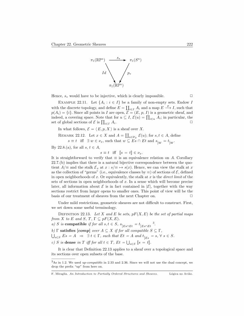
Chapter 22. Geometric Sheaves 222
π1(RPn) - π1(Sn)
Id p∗
π1(RPn)
s∗
AAAAAU
Hence, s∗ would have to be injective, which is clearly impossible. 2
Example 22.11. Let Ai : i ∈ I be a family of non-empty sets. Endow I
with the discrete topology, and define E =∐i∈I Ai and a map E
p−→ I, such thatp(Ai) = i. Since all points in I are open, E = (E, p, I) is a geometric sheaf, andindeed, a covering space. Note that for u ⊆ I, E(u) =
∏i∈u Ai; in particular, the
set of global sections of E is∏i∈I Ai. 2
In what follows, E = 〈E, p,X 〉 is a sheaf over X.
Remark 22.12. Let x ∈ X and A =∐u∈νx E(u); for s, t ∈ A, define
s ≡ t iff ∃ w ∈ νx, such that w ⊆ Es ∩ Et and s|W = t|W .
By 22.8.(a), for all s, t ∈ A,
s ≡ t iff [[s = t]] ∈ νx.
It is straightforward to verify that ≡ is an equivalence relation on A. Corollary22.7.(b) implies that there is a natural bijective correspondence between the quo-tient A/≡ and the stalk Ex at x : s/≡ 7→ s(x). Hence, we can view the stalk at xas the collection of “germs” (i.e., equivalence classes by ≡) of sections of E , definedin open neighborhoods of x. Or equivalently, the stalk at x is the direct limit of thesets of sections in open neighborhoods of x. In a sense which will become preciselater, all information about E is in fact contained in |E|, together with the waysections restrict from larger opens to smaller ones. This point of view will be thebasis of our treatment of sheaves from the next Chapter on. 2
Under mild restrictions, geometric sheaves are not difficult to construct. First,we set down some useful terminology.
Definition 22.13. Let X and E be sets, pF (X,E) be the set of partial mapsfrom X to E and S, T , Γ ⊆ pF (X,E).
a) S is compatible if for all s, t ∈ S, s|Es∩Et = t|Es∩Et3.
b) Γ satisfies [comp] over A ⊆ X if for all compatible S ⊆ Γ,⋃s∈S Es = A ⇒ ∃ t ∈ Γ, such that Et = A and t|Es = s, ∀ s ∈ S.
c) S is dense in T iff for all t ∈ T , Et =⋃s∈S [[s = t]].
It is clear that Definition 22.13 applies to a sheaf over a topological space andits sections over open subsets of the base.
3As in 1.2. We used up-compatible in 2.33 and 2.36. Since we will not use the dual concept, wedrop the prefix “up” from here on.
F. Miraglia. An Introduction to Partially Ordered Structures and Sheaves. Logica no Aviao.
Chapter 22. Geometric Sheaves 223
Proposition 22.14. Let p : E−→ X be a map, where X is a topologicalspace and E is a set. Suppose Γ ⊆ pF (X,E) satisfies
(1) For all s ∈ Γ, Es =def doms is open in X;
(2) All elements of Γ are sections of p, i.e., p s = IdEs;
(3) For all s, t ∈ Γ, [[s = t]] is open in X;
(4) For all e ∈ E, there is s ∈ Γ such that e ∈ Ims.
Then, there is a unique topology on E, such that p is a local homeomorphism.Moreover, if E = 〈E, p,X 〉 is the sheaf so determined over X, then
a) Γ ⊆ |E| and Γ is dense in |E|.b) Let B be a basis for the topology on X. For v ∈ Ω(X), define
ΓB, v = s|w : w ⊆ v and w ∈ B and Γ(v) = s ∈ Γ : Es = v.If, for u ∈ Ω(X), ΓB, u satisfies [comp] over u, then Γ(u) = E(u).
Proof. Let B = s(u ∩ Es) : 〈 s, u 〉 ∈ Γ × Ω(X); it is straightforwardto show that for all s, s′ ∈ Γ and u, v ∈ Ω(X),
(*) s(u ∩ Es) ∩ s′(v ∩ Es′) = s([[s = s′]] ∩ u ∩ v).
Thus, B is closed under finite intersections and is a basis for a topology on E. Notethat all s ∈ Γ are open in this topology (by definition !). Further, from (*) oneeasily verifies that for all s, s′ ∈ Γ and v ∈ Ω(X),
s−1(s′(v ∩ Es′) = [[s = s′]] ∩ v,
that is open in X. Thus, all s ∈ Γ are continuous, open and injective from theopen set Es ⊆ X, onto the open set Ims ⊆ E. Therefore, every s ∈ Γ is a home-omorphism from the open Es in X, onto the open Ims in E. Hence, assumption(4) implies that p is a local homeomorphism and E = 〈E, p,X 〉 is a sheaf, with Γ⊆ |E|.
To show that Γ is dense in |E|, let t ∈ |E|, x ∈ Et and e = t(x). By (4), thereis s ∈ Γ such that e = s(z) ∈ Ims. Since t and s are sections of p, we get x = z.Since E is a sheaf, [[s = t]] ∈ νx. Hence, Et =
⋃s∈Γ [[s = t]], as desired.
Clearly, Γ(u) ⊆ E(u); for the reverse inclusion, fix a basis B for the topol-ogy on X and a section t ∈ E(u). By denseness, there is S ⊆ Γ, such thatEt =
⋃s∈S [[s = t]]. Since B is basis for the topology on X and all [[s = t]] are
open in X, we can write
Et =⋃i∈I wi,
where, for each i ∈ I, there is s ∈ S such that wi ⊆ [[s = t]]. Thus, for i ∈ I ands ∈ S,
s|wi = t|wi , s|wi ∈ Γu and Es|wi = wi.
Since ΓB, u satisfies [comp] over u, there is s′ ∈ Γ such that
s′|wi = s|wi = t|wi and Es′ = u.
Now, item (4) in 22.8.(b) yields s′ = t, i.e., t ∈ Γ(u).
Perhaps the best way to understand 22.14 is to see it in action.
F. Miraglia. An Introduction to Partially Ordered Structures and Sheaves. Logica no Aviao.

Chapter 22. Geometric Sheaves 224
Example 22.15. Let H be a HA and let X = S(H) be the Stone space of H(19.2). Define E =
∐F∈X H/F and p : E −→ X, by sending all elements of the
quotient H/F to the prime filter F in X. Observe that p is onto X. Each a ∈ Hgives rise to a global section of p as follows :
a ∈ H 7−→ a∗ : X −→ E, where a∗(F ) = a/F .
Let Γ = a∗ : a ∈ H; clearly, conditions (1), (2) and (4) are satisfied by Γ.Regarding (3), recall (6.10) that if a, b ∈ H, then
(a ↔ b) = (a → b) ∧ (b → a) = max z ∈ H : a ∧ z = b ∧ zexists in H and that for all t ≤ (a ↔ b), we have t ∧ a = t ∧ b. For a and b ∈ H,
[[a∗ = b∗]] = F ∈ X : a/F = b/F= F ∈ X : ∃ c ∈ F such that a ∧ c = b ∧ c= F ∈ X : (a ↔ b) ∈ F = Sa↔b,
which is open in X. 22.14 applies, yielding a sheaf E = 〈E, p, S(H) 〉, with Γ densein |E|.
Next, we show that if B = Sa : a ∈ H is the standard basis of opens forS(H), then ΓB,X has [comp] over X. From this and 22.14.(b) we conclude that
Γ = Γ(X) = E(X),
that is, the set of global sections of E is an isomorphic copy of H. Let S ⊆ Γ andus = Scs , s ∈ S, be basic opens in S(H) such that⋃
s∈S us = X and s|us : s ∈ S is compatible in E .
Since X is compact (19.8), there is T ⊆f S, with⋃t∈T ut = X. Note that if we
can find a ∈ H such that a∗|ut = t|ut , for all t ∈ T , then, by the compatibility of
S, we get a∗|us = s|us , for all s ∈ S. Hence, we may assume that S is finite, S =
a∗i : 1 ≤ i ≤ n, with ua∗i = Sci , 1 ≤ i ≤ n. The compatibility of a∗i |Scimeans
that for all i, j ≤ n, we have
Sci∧cj = Sci ∩ Scj ⊆ [[a∗i = a∗j ]] = Sai↔aj .
Thus, 19.5.(b) entails that for i, j ≤ n, ci ∧ cj ≤ (ai ↔ aj); in particular,
(*) ai ∧ (ci ∧ cj) = aj ∧ (ci ∧ cj),for all i, j ≤ n. Define a =
∨ni=1 ai ∧ ci; for each i ≤ n, (*) yields
a ∧ ci = (ai ∧ ci) ∨∨i6=j ci ∧ cj ∧ aj ≤ ai ∧ ci,
wherefrom it follows that a ∧ ci = ai ∧ ci. Consequently, if F is a prime filterin H such that ci ∈ F , then a/F = ai/F , that is, a∗ restricted to Sci is equalto ai restricted to the same basic open. Hence, ΓB,X satisfies [comp] over X, asasserted. 2
Corollary 22.16. Every Heyting algebra can be identified with the set of theglobal sections of a sheaf of Heyting algebras over its Stone space. 2
Example 22.17. Let R be a commutative ring with identity, which for ease ofexposition, we assume to be an integral domain. For each prime ideal P ∈ Spec(R),let RP be the localization of R at P (9.41), that is, RP is the ring of fractions a/r,such that a ∈ R and r 6∈ P . Since R is an integral domain 4, in RP
4xy = 0 iff x = 0 or y = 0; equivalently, (0) is a prime ideal.
F. Miraglia. An Introduction to Partially Ordered Structures and Sheaves. Logica no Aviao.
Chapter 22. Geometric Sheaves 225
a/r = b/s iff as = bt.
Let E =∐P∈Spec(R) RP and define p : E −→ Spec(R) by sending each element
of the localization RP to the point P in Spec(R). Clearly, p is surjective. Eachelement of E is of the form a/b, with a ∈ R and b outside some prime ideal in R.
Recall from Chapter 19, that Zr = P ∈ Spec(R) : r 6∈ P is the compactopen associated to r ∈ R and that B = Zr : r ∈ R is a basis for the Zariskitopology on Spec(R). Further, since R is an integral domain, Zr = ∅ iff r = 0. Toeach pair 〈 a, r 〉 ∈ R × (R− 0) we can associate a map
a/r : Zr −→ E, given by P ∈ Zr 7→ a/r ∈ RP ,
that is well defined, because for all P ∈ Zr, r 6∈ P . Hence, a/r is a section of pover its domain, Zr.
Let Γ = a/r : 〈 a, r 〉 ∈ R × (R− 0). The set of elements in Γ whose extentequals Spec(R) = Z1 is
Γ(Spec(R)) = a/1 : a ∈ R,an isomorphic copy of R. Since R is a domain, Γ may be identified with the field ofquotients of R, together with the assignment to each fraction, of the set of primesthat do not contain its denominator.
Clearly, Γ satisfies conditions (1), (2) and (4) of 22.14. Further, Γ is closedunder restrictions of its elements to basic opens in Spec(R) : if a/r ∈ Γ andZs ⊆ Zr, then (a/r)|Zs = as/rs, since, by 19.5.(a), we have Zs = Zr ∩ Zs = Zrs.
In particular, ΓB,X ⊆ Γ. For condition (3), it is straightforward to see that
(∗) [[a/r = b/s]] =
Zr ∩ Zs if as = br∅ otherwise
Hence, [[a/r = b/s]] is open in Spec(R), for all a/r, b/s ∈ Γ. By 22.14, we have asheaf E = 〈E, p, Spec(R) 〉, with Γ dense in |E|.
We now verify that if ai/ri, i ∈ I, is a compatible collection of sections in Γ,such that
⋃Zri = Spec(R), then there is a ∈ R such that (a/1)|Zri
= ai/ri, for
all i ∈ I. Thus, ΓB,Spec(R) will satisfy [comp] over Spec(R), and
Γ(Spec(R)) = a/1 : a ∈ R = E(R).
What is the meaning of a/r being compatible with b/s ? The fact that R is anintegral domain implies that the zero ideal, (0), is prime. Since it is contained in
every prime ideal, (0) is a generic point for Spec(R), that is, (0) = Spec(R). Butthis means that (0) is in every non-empty open in Spec(R), and so the intersectionof any finite number of non-empty opens in Spec(R) is non-empty. Since r, s 6= 0implies Zr ∩ Zs 6= ∅, from (*) we get that for all a, b ∈ R and r, s ∈ R− 0(**) a/r is compatible with b/s iff as = br.
Let ai/ri, i ∈ I, be a compatible subset of Γ, with⋃Zri = Spec(R). By Corollary
19.9, there is J ⊆f I, such that the ideal generated by the rj , j ∈ J , is equal toR. Hence, there are αj ∈ R such that∑
j∈J αjrj = 1. (1)
Since the sections ai/ri are compatible, from (**) we get
∀ i, k ∈ I, airk = akri. (2)
F. Miraglia. An Introduction to Partially Ordered Structures and Sheaves. Logica no Aviao.
Chapter 22. Geometric Sheaves 226
Define a =∑j∈J αjaj ; for each i ∈ I, (1) and (2) yield
ri a = ri∑j∈J αjaj =
∑j∈J αjajri =
∑j∈J αjrjai = ai (
∑j∈J αjrj)
= ai.
Hence, the value of a/1 in each localization RP , P ∈ Zri , is the same as ai/ri, andso a/1 is the “gluing” of the compatible family given at the outset.
With only slight modifications, one can show that the set of elements in Γwith domain Zr is equal to E(Zr), for all r 6= 0 in R. Further, essentially the sameargument shows that an analogous construction holds for any module over R,with stalks that are the localizations of the module at each prime in Spec(R). 2
Corollary 22.18. Every integral domains can be identified with the set ofglobal sections of a sheaf of local rings over its Zariski spectrum. 2
Corollary 22.18 is true for all commutative rings with identity, as will be seenin the Example 27.21 and Theorem 27.22, due to A. Grothendieck.
Example 22.19. Let R be a commutative regular ring (19.19). By Theorem20.2, every prime ideal in R is maximal. Hence, R/P is a field, for all P ∈ Spec(R),and so if e is an idempotent in R, e/P = 0 or e/P = 1.
By 19.22, Spec(R) is a Boolean space, wherein B = Zr : r ∈ R is a basis ofclopens. Further, if er is the unique idempotent of R such that (r) = (er), thenZr = Zer . Since R has no nilpotent elements, the intersection of all primes in R isequal to 0. The set of ideas presented below are due to R. S. Pierce ([57], [6]).
Let E =∐P∈ Spec(R) R/P and define p : E −→ Spec(R) by assigning to each
element of R/P the point P ∈ Spec(R). Each a ∈ R defines a map (to be indicatedby the same symbol)
a : Spec(R) −→ E, given by P 7→ a/P .
Clearly, every such map is a section of p. Let Γ be the set of sections of p overSpec(R), just defined. We have
[[a = b]] = P ∈ Spec(R) : a/P = b/P = P ∈ Spec(R) : (a− b) ∈ P= complement of Z(a−b) in Spec(R),
which is clopen in Spec(R). It is now straightforward to see that Γ has properties(1) − (4) of 22.14. Hence, E = 〈E, p, Spec(R) 〉 is a sheaf, with Γ dense in |E|. Wewish to show that Γ = E(Spec(R)). As a preliminary step, we prove
Fact 1. Let a, b ∈ R and let e, f be idempotents in R. Then
a) Ze ⊆ [[a = b]] iff ae = be.
b) [[a|Ze = b|Zf ]] = [[a = b]] ∩ Ze ∩ Zf = [[a = b]] ∩ Zef .
c) a|Ze is compatible with b|Zf iff aef = bef .
Proof. (a) Let P be a prime ideal in R. If e 6∈ R and (ae−be) = 0, then, (a− b) ∈ P ,and so P ∈ [[a = b]], proving that Ze ⊆ [[a = b]]. Now assume that Ze ⊆ [[a = b]];we show that ae = be by proving that it is in every prime ideal in R. We maysuppose that e 6∈ P ; then P ∈ Ze, and so a/P = b/P , whence (a − b) ∈ P . Butthen, (ae− be) = 0, as desired. Items (b) and (c) are left to the reader 5.
5Compare with 22.30.(c).
F. Miraglia. An Introduction to Partially Ordered Structures and Sheaves. Logica no Aviao.
Chapter 22. Geometric Sheaves 227
Suppose ai ∈ Γ and clopens Zei , i ∈ I, verify
(1) The restrictions of the ai to Zei are compatible, that is
∀ i, j ∈ I, [[ai|Zei= aj |Zej
]] = Zei ∩ Zej(2)
⋃i∈I Zei = Spec(R).
We may suppose that each ei is an idempotent. (1) and Fact 1 yield
(*) ∀ i, k ∈ I, aieiek = akekei.
As in the 22.15 and 22.17, condition (2) yields a finite J ⊆ I and cj ∈ R, suchthat
(**)∑j∈J cjej = 1.
Define a =∑j∈J cjajej ; for each i ∈ I, (*) and (**) yield
aei = ei∑j∈J cjajej =
∑j∈J cjajejei =
∑j∈J cjaieiej = aiei
∑j∈J cjej
= aiei,
and so, [[a = ai|ei ]] = Zei , for all i ∈ I, as desired. 2
Corollary 22.20. Every commutative regular ring can be identified with theset of global sections of a sheaf of fields over its spectrum. 2
Remark 22.21. The last three examples consist of just a glimpse of what isknown as “representation of algebras by continuous sections”. A classical referenceis [29]. Recent examples also appear in [3]. 2
A geometric sheaf E = 〈E, p,X 〉 is Hausdorff if E is a Hausdorff space. Thesituation in Example 22.19 is quite typical :
Lemma 22.22. For a sheaf E = 〈E, p,X 〉 over a Hausdorff space X, thefollowing are equivalent :
(1) E is Hausdorff.
(2) For all u ∈ Ω(X) and s, t ∈ E(u), [[s = t]] is clopen in u.
(3) For all s, t ∈ |E|, [[s = t]] is clopen in Es ∩ Et.
Proof. (1) ⇒ (2) : It is enough to show that
x ∈ u : s(x) 6= t(x) = u− [[s = t]]
is open in u. If x ∈ (u − [[s = t]]), since s(x) = e 6= t(x) = e′, there are V ∈ νe andV ′ ∈ νe′ , such that V ∩ V ′ = ∅ and p restricted to V and V ′ are homeomorphismsonto p(V ) and p(V ′), respectively. Hence, the intersection p(V ) ∩ p(V ′) is non-empty and contained in (u − [[s = t]]), as needed. (2) ⇒ (1) is immediate froms|[[s=t]] = t|[[s=t]] (22.30.(a)).
(3) ⇒ (1) : Given distinct e, e′ ∈ E, we have two cases :
∗ p(e) 6= p(e′). Let u and v be disjoint open neighborhoods of p(e) and p(e′),respectively. There are U ∈ νe and V ∈ νe′ , such that p is a homeomorphism of Uand V onto p(U) ⊆ u and p(V ) ⊆ v, respectively. Clearly, U ∩ V = ∅.∗ p(e) = p(e′) = x. Again, there are U ∈ νe and U ′ ∈ νe′ , such that p|U and p|U ′are homeomorphisms onto p(U), p(U ′). Let v = p(U) ∩ p(U ′), let s be the inverse
F. Miraglia. An Introduction to Partially Ordered Structures and Sheaves. Logica no Aviao.
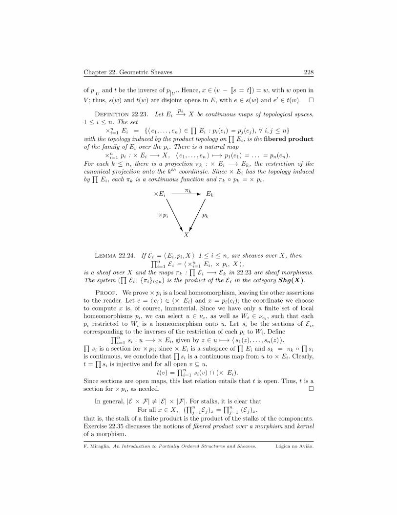
Chapter 22. Geometric Sheaves 228
of p|U and t be the inverse of p|U ′ . Hence, x ∈ (v − [[s = t]]) = w, with w open in
V ; thus, s(w) and t(w) are disjoint opens in E, with e ∈ s(w) and e′ ∈ t(w).
Definition 22.23. Let Eipi−→ X be continuous maps of topological spaces,
1 ≤ i ≤ n. The set
×ni=1 Ei = 〈 e1, . . . , en 〉 ∈∏Ei : pi(ei) = pj(ej), ∀ i, j ≤ n
with the topology induced by the product topology on∏Ei, is the fibered product
of the family of Ei over the pi. There is a natural map
×ni=1 pi : × Ei −→ X, 〈 e1, . . . , en 〉 7−→ p1(e1) = . . . = pn(en).
For each k ≤ n, there is a projection πk : × Ei −→ Ek, the restriction of thecanonical projection onto the kth coordinate. Since × Ei has the topology inducedby∏Ei, each πk is a continuous function and πk pk = × pi.
×Ei - Ek
×pi pk
X
πk
AAAAAU
Lemma 22.24. If E i = 〈Ei, pi, X 〉 1 ≤ i ≤ n, are sheaves over X, then∏ni=1 E i = 〈×ni=1 Ei, × pi, X 〉,
is a sheaf over X and the maps πk :∏E i −→ Ek in 22.23 are sheaf morphisms.
The system (∏E i, πii≤n) is the product of the E i in the category Shg(X).
Proof. We prove × pi is a local homeomorphism, leaving the other assertionsto the reader. Let e = 〈 ei 〉 ∈ (× Ei) and x = pi(ei); the coordinate we chooseto compute x is, of course, immaterial. Since we have only a finite set of localhomeomorphisms pi, we can select u ∈ νx, as well as Wi ∈ νei , such that eachpi restricted to Wi is a homeomorphism onto u. Let si be the sections of E i,corresponding to the inverses of the restriction of each pi to Wi. Define∏n
i=1 si : u −→ × Ei, given by z ∈ u 7−→ 〈 s1(z), . . . , sn(z) 〉.∏si is a section for × pi; since × Ei is a subspace of
∏Ei and sk = πk
∏si
is continuous, we conclude that∏si is a continuous map from u to × Ei. Clearly,
t =∏si is injective and for all open v ⊆ u,
t(v) =∏ni=1 si(v) ∩ (× Ei).
Since sections are open maps, this last relation entails that t is open. Thus, t is asection for × pi, as needed.
In general, |E × F| 6= |E| × |F|. For stalks, it is clear that
For all x ∈ X, (∏nj=1Ej)x =
∏nj=1 (Ej)x.
that is, the stalk of a finite product is the product of the stalks of the components.Exercise 22.35 discusses the notions of fibered product over a morphism and kernelof a morphism.
F. Miraglia. An Introduction to Partially Ordered Structures and Sheaves. Logica no Aviao.
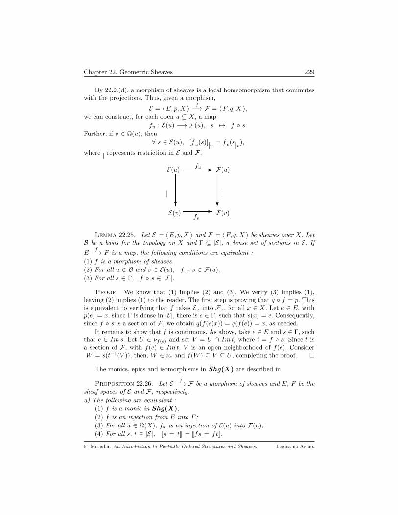
Chapter 22. Geometric Sheaves 229
By 22.2.(d), a morphism of sheaves is a local homeomorphism that commuteswith the projections. Thus, given a morphism,
E = 〈E, p,X 〉 f−→ F = 〈F, q,X 〉,we can construct, for each open u ⊆ X, a map
fu : E(u) −→ F(u), s 7→ f s.Further, if v ∈ Ω(u), then
∀ s ∈ E(u), [fu(s)]|v = fv(s|v),where | represents restriction in E and F .
E(v)
E(u)
?
- F(u)
|
fu
F(v)
|
fv
?-
Lemma 22.25. Let E = 〈E, p,X 〉 and F = 〈F, q,X 〉 be sheaves over X. LetB be a basis for the topology on X and Γ ⊆ |E|, a dense set of sections in E. If
Ef−→ F is a map, the following conditions are equivalent :
(1) f is a morphism of sheaves.
(2) For all u ∈ B and s ∈ E(u), f s ∈ F(u).
(3) For all s ∈ Γ, f s ∈ |F|.
Proof. We know that (1) implies (2) and (3). We verify (3) implies (1),leaving (2) implies (1) to the reader. The first step is proving that q f = p. Thisis equivalent to verifying that f takes Ex into Fx, for all x ∈ X. Let e ∈ E, withp(e) = x; since Γ is dense in |E|, there is s ∈ Γ, such that s(x) = e. Consequently,since f s is a section of F , we obtain q(f(s(x)) = q(f(e)) = x, as needed.
It remains to show that f is continuous. As above, take e ∈ E and s ∈ Γ, suchthat e ∈ Ims. Let U ∈ νf(e) and set V = U ∩ Im t, where t = f s. Since t isa section of F , with f(e) ∈ Im t, V is an open neighborhood of f(e). ConsiderW = s(t−1(V )); then, W ∈ νe and f(W ) ⊆ V ⊆ U , completing the proof.
The monics, epics and isomorphisms in Shg(X) are described in
Proposition 22.26. Let E f−→ F be a morphism of sheaves and E, F be thesheaf spaces of E and F , respectively.
a) The following are equivalent :
(1) f is a monic in Shg(X);
(2) f is an injection from E into F ;
(3) For all u ∈ Ω(X), fu is an injection of E(u) into F(u);
(4) For all s, t ∈ |E|, [[s = t]] = [[fs = ft]].
F. Miraglia. An Introduction to Partially Ordered Structures and Sheaves. Logica no Aviao.

Chapter 22. Geometric Sheaves 230
b) The following are equivalent :
(1) f is an epic in Shg(X); (2) f is a surjection of E onto F ;
(3) Imf is dense in |F|.c) The following are equivalent :
(1) f is an isomorphism in Shg(X);
(2) f is a homeomorphism from E onto F .
Proof. (a) Clearly, (2) ⇒ (1); for the converse, we use the fibered productof E over f (22.35); in the notation therein, we have f d1 = f d2, which forcesd1 = d2. But this means that f(e) = f(e′) implies e = e′, and f is an injectionfrom E into F . The remainder of (a) is left to the reader.
(b) Clearly, (2) → (1); we prove that (3) ⇔ (2), leaving (1) ⇒ (2) as an exercise.To fix notation, assume that E = 〈E, p,X 〉 and F = 〈F, q,X 〉.(3) ⇒ (2) : Fix y ∈ F ; let x = q(y) and let t be a section of F over some open
u ∈ νx, such that t(x) = y. By (3), Et =⋃s∈|E [[fs = t]], and so for some s ∈ |E|,
x ∈ [[fs = t]]. Hence, f(s(x)) = t(x) = y and f is onto F .
(2) ⇒ (3) : Let t ∈ F(u) be a section of F over u. Since f is surjective, for x ∈ u,
there is ex ∈ E, such that f(ex) = t(x). For x ∈ u, select sx ∈ |E| such that
∗ Esx ∈ νx ∩ Ω(u) and ∗ sx(x) = ex.
Since f(sx(x)) = t(x), x ∈ u, we have that [[(f sx) = t]] = ux are non-empty opensin X, satisfying Et = u =
⋃x∈u ux, and (3) follows. Item (c) is straightforward
and left to the reader.
Remark 22.27. By 22.26.(a), the subsheaves of a geometric sheaf can beidentified, up to isomorphism, to the open sets of its sheaf space. Thus, the familyof subsheaves of E = 〈E, p,X 〉 is 〈U, p|U , X 〉 : U ∈ Ω(E). 2
Remark 22.28. A sheaf morphism may be an epimorphism in Shg(X),although the maps fu are not surjections. It is this fact that produces the differentCohomology Theories that are such an important part of sheaf theory and itsapplications. 2
By 22.26.(a), if E is a subsheaf of F (written E ⊆ F), then for each u ∈ Ω(X),
there is a natural injection, E(u)fu−→ F(u), such that for all open v ⊆ u, the
following diagram is commutative :
E(v)
E(u)
?
- F(u)
|
fu
F(v)
|
fv
?-
Furthermore, since E is a sheaf, any compatible family of sections in |E| can be“glued” to a section in E .
F. Miraglia. An Introduction to Partially Ordered Structures and Sheaves. Logica no Aviao.

Chapter 22. Geometric Sheaves 231
Exercises
22.29. Let E = 〈E, p,X 〉 be a sheaf over X.
a) Prove that condition (4) in 22.8.(b) is equivalent to
If s, t ∈ E(u) are such that s|ui = t|ui , for i ∈ I, then s = t.
b) Let ui : i ∈ I ⊆ Ω(X), u =⋃
ui and si ∈ E(ui), i ∈ I. Prove that thestatement in 22.8.(c) is equivalent to
If si|(ui∩uj) = sj |(ui∩uj), ∀ i, j ∈ I, then
there is a unique s ∈ E(u), such that s|ui = si, ∀ i ∈ I.2
22.30. Let a, b ∈ |E|, where E = 〈E, p,X 〉 be a sheaf over X. With notationas in 22.8,
a) a|[[a=b]]= b|[[a=b]]
.
b) [[a = b]] is the largest open set u ⊆ (Ea∩Eb) such that a|u = b|u.
c) If u, v are opens in Ea and Eb, respectively, then
[[a|u = b|v]] = u ∩ v ∩ [[a = b]]. 2
22.31. a) For S, T ⊆ pF (X,E) show that S is dense in T iff for all t ∈ T ,there is B ⊆ S such that Et =
⋃b∈B [[s = b]].
b) If E = 〈E, p,X 〉 is a sheaf over X and S, T ⊆ |E|, S is dense in T iff for allt ∈ T there is 〈ui, si 〉 : i ∈ I ⊆ Ω(X) × S, such that
(1) Et =⋃ui and (2) t|ui = si|Esi∩ui , ∀ i ∈ I. 2
22.32. If X is a topological space, Ω(X) can be represented as the set of globalsections of a geometric sheaf over X, whose stalks are Ω(X)/νx, x ∈ X. 2
22.33. Let E be the sheaf of 22.19, with the convention of not distinguishingbetween elements of Γ and R. Show that
a) If s ∈ E(Zr), then s = a|Zr , for some a ∈ Γ.
b) For all s, t ∈ E , if Es and Et are clopen in Spec(R), then [[s = t]] is clopen inSpec(R).
c) If P is a prime ideal in a commutative regular ring R, then the localization ofR at P (9.41), RP , is naturally isomorphic to the residue field R/P . 2
22.34. a) In the situation of 22.24, show that for each u ∈ Ω(X), there is abijective map
ηu : [∏E i](u) −→
∏Ei(u),
such that for all open v, u ∈ Ω(X), if v ⊆ u, then the following diagram is com-mutative, where | is the restriction map in the sheaf
∏E i, while |
n is the product
of the restriction maps on each E i :
F. Miraglia. An Introduction to Partially Ordered Structures and Sheaves. Logica no Aviao.
Chapter 22. Geometric Sheaves 232
[∏Ei](v)
[∏Ei](u)
?
-∏Ei(u)
|
ηu
∏Ei(v)
|n
ηv
?-
b) Is it possible to use 22.14 to give a proof of 22.24 ? 2
22.35. Let E = 〈E, p,X 〉 f−→ F = 〈F, q,X 〉 be a morphism of sheaves overX. Define the fibered product of E over f by
E ×f E = 〈 e, e′ 〉 ∈ E × E : f(e) = f(e′),with the topology induced by E × E. Note that for all 〈 e, e′ 〉 ∈ E ×f E we havep(e) = p(e′). Thus, 〈 e, e′ 〉 7→ p(e) defines a map from E ×f E to X, writtenρ. We also have projections d1, d2 from E ×f E to E, given by the restrictionof the projections defined on E × E onto the first and the second coordinates,respectively. Clearly, these are continuous functions. Then :
a) E ×f E is open in E × E.
b) ρ is the restriction of p× p to E ×f E. Conclude that E ×f E = 〈E ×f E, ρ,X 〉is a sheaf over X.
c) d1 and d2 are the restriction to E ×f E of the canonical projections fromE × E −→ E, described in 22.24. Conclude that they are sheaf morphisms fromE ×f E to E . Verify that f d1 = f d2.
In the above situation, if f = IdE then we obtain a sheaf, indicated by ∆E ,which corresponds to the graph of the identity relation on E . 2
22.36. a) LetK be a closed set in a topological space Y . Let Z = Y ∪ (∗ × K)be the disjoint union Y and K, with the following topology :
(1) The topology on Y is its original topology.
(2) An open neighborhood of 〈 ∗, z 〉 ∈ (∗ × K) is an open neighborhood V of zin Y , with 〈 ∗, z 〉 in place of z : (V − z) ∪ 〈 ∗, z 〉.
Let 〈Y, p,X 〉 be a sheaf over X.
a) Define Zq−→ X by q|Y = p and q(∗, z) = p(z); then 〈Z, q,X 〉 is a sheaf over
X and Yh−→ Z, given by h(y) = y, is a sheaf morphism.
b) Show that k : Y −→ Z, given by
k(z) =
z if z 6∈ K〈 ∗, z 〉 if z ∈ K,
is a sheaf morphism and prove that (1) ⇔ (2) in 22.26.(b). 2
The following Exercise indicate how Examples 22.15, 22.17 and 22.19 do infact yield algebraic representation results.
22.37. Notation as in 22.15, let E = 〈E, p, S(H) 〉 be the sheaf constructedtherein. There are global sections >∗ and ⊥∗, defined, for F ∈ S(H), by
F. Miraglia. An Introduction to Partially Ordered Structures and Sheaves. Logica no Aviao.

Chapter 22. Geometric Sheaves 233
>∗(F ) = >/F and ⊥∗(F ) = ⊥/F .
Define ∧, ∨ : E × E −→ E as follows :
For 〈 e, e′ 〉 ∈ (E×E), with p(e) = p(e′) = F ∈ S(H), write e = a/F ande′ = b/F , with a, b ∈ H and set
∧(e, e′) = a/F ∧ b/F = (a ∧ b)/F∨(e, e′) = a/F ∨ b/F = (a ∨ b)/F .
Define ≤ = 〈 a/F, b/F 〉 ∈ E × E : a/F ≤ b/F in H/F, together with a projec-tion on S(H), corresponding to the restriction of p × p to ≤. Then :
a) ≤ is a subsheaf of E × E , and the maps ∧, ∨ are well-defined sheaf morphisms.
b) For each open u in S(H), the set of sections over u, E(u), inherits
(i) a binary relation ≤(u), the set of sections of ≤ over u;
(ii) two binary operations, namely ∧u and ∨u.
(iii) two distinguished elements >∗|u, ⊥∗|u.
With this structure, E(u) is a HA. Further, the restriction map E(u) −→ E(v),v ⊆ u, are HA-morphisms.
c) For each a ∈ H there is a HA-isomorphism, γa : E(Sa) −→ H/a→, such thatfor all b ≤ a the following diagram is commutative :
E(Sb)
E(Sa)
?
- H/a→
|
γa
H/b→
αab
γb
?-
where αab is the HA-morphism αab(x/a→) = x/b→, x ∈ H.
e) The map constructed in 22.15 is a lattice isomorphism from H onto the latticeof global sections of E . 2
22.38. With Exercise 22.37 as a model, discuss Examples 22.17 and 22.19, toshow that integral domains and commutative regular rings are ring isomorphic tothe rings of global sections of the sheaves constructed in those Examples. 2
22.39. How would one define a first-order structure in the category of geo-metric sheaves ? 2
F. Miraglia. An Introduction to Partially Ordered Structures and Sheaves. Logica no Aviao.
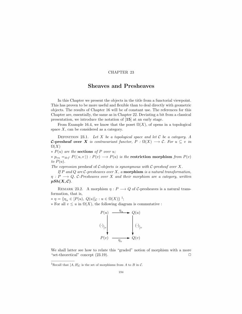
CHAPTER 23
Sheaves and Presheaves
In this Chapter we present the objects in the title from a functorial viewpoint.This has proven to be more useful and flexible than to deal directly with geometricobjects. The results of Chapter 16 will be of constant use. The references for thisChapter are, essentially, the same as in Chapter 22. Deviating a bit from a classicalpresentation, we introduce the notation of [15] at an early stage.
From Example 16.4, we know that the poset Ω(X), of opens in a topologicalspace X, can be considered as a category.
Definition 23.1. Let X be a topological space and let C be a category. AC-presheaf over X is contravariant functor, P : Ω(X) −→ C. For u ⊆ v inΩ(X)
∗ P (u) are the sections of P over u;
∗ pvu =def P (〈u, v 〉) : P (v) −→ P (u) is the restriction morphism from P (v)to P (u).
The expression presheaf of C-objects is synonymous with C-presheaf over X.
If P and Q are C-presheaves over X, a morphism is a natural transformation,η : P −→ Q. C-Presheaves over X and their morphism are a category, writtenpSh(X, C).
Remark 23.2. A morphism η : P −→ Q of C-presheaves is a natural trans-formation, that is,
∗ η = ηu ∈ [P (u), Q(u)]C : u ∈ Ω(X) 1;
∗ For all v ≤ u in Ω(X), the following diagram is commutative :
P (v)
P (u)
?
- Q(u)
(·)|v
ηu
Q(v)
(·)|v
ηv
?-
We shall latter see how to relate this “graded” notion of morphism with a more“set-theoretical” concept (23.19). 2
1Recall that [A,B]C is the set of morphisms from A to B in C.
234

Chapter 23. Sheaves and Presheaves 235
Example 23.3. If C has a final object, 1, we may define a presheaf over X,also indicated by 1, as follows : for all u ∈ Ω(X),
1(u) = 1 and the restriction maps are the identity morphism of 1.
It is clear that 1 is the final object in pSh(X, C). Similar comments apply whenC has an initial object or a zero. 2
Remark 23.4. It is clear that a presheaf of C-objects can also be defined asa covariant functor from Ω(X)op to C, where ∗op is the dual category as in 16.5.Many texts on the subject adopt this definition.
If P : Ω(X)op −→ C is a presheaf, then with the notation of 23.1, observe thatif u ⊆ v ⊆ w in Ω(X), then functoriality entails
(1) puu = IdP (u) and (2) pwu = pvu pwv.Moreover, P (∅) must be an object in C such that [P (u), P (∅)] 6= ∅, for all u ∈ Ω(X).Whenever C has a final object, 1, it is standard to set
P (∅) = 1,
a convention we shall also adopt. The following table exemplifies the terminologyin 23.1, with notation as in 16.3 :
Usual Name Functor from Ω(X)op to
Presheaf of sets over X Set
Presheaf of partial orders over X Po
Presheaf of distributive lattices DPresheaf of Abelian groups over X AbGr
Presheaf of rings over X CR
Presheaf of L-structures over X L-mod
There is something in common with all the examples in the preceding table : allare set-based categories (16.1), the only type of category that will be target ofpresheaves in this book. 2
23.5. Conventions. a) From here on, the term category will mean set-basedcategory, that is, sets underlie its objects and maps underlie its morphisms.
b) If P : Ω(X)op −→ C is a C-presheaf over X, then
(1) P (∅) = ∗, a fixed singleton;
(2) If u ∈ Ω(X) and s ∈ P (v), define s|u = pv,u∩v(s).
Note that if u ⊆ v in Ω(X) and x ∈ P (v), then x|u = pvu(s). Hence, the operation
(·)|u generalizes the restriction morphisms in a presheaf.
(3) For u, v ∈ Ω(X), u ≤ v stands for v ∈ Ω(X) and u ∈ Ω(v). 2
Definition 23.6. Let P : Ω(X)op −→ C be a C-presheaf over X.
a) The domain of P is the set |P | =∐u∈Ω(X) P (u).
b) For s ∈ |P |, the extent of s in P is defined as
F. Miraglia. An Introduction to Partially Ordered Structures and Sheaves. Logica no Aviao.

Chapter 23. Sheaves and Presheaves 236
EP s = the unique u ∈ Ω(X) such that s ∈ P (u).
c) If S ⊆ |P |, the support of S is defined as
EPS =⋃s∈S Es.
d) For s, t ∈ |P |, define 2
[[s = t]]P =⋃u ≤ (Es ∩ Et) : s|u = t|u,
called the equality of P . Note that [[s = t]]P ∈ Ω(X).
e) P is extensional 3 if for all s, t ∈ |P |,[ext] EP s = EP t = [[s = t]]P ⇔ s = t.
Context allowing, we omit P from the notation of extent, support and equality.
Proposition 23.7. Let P be a C-presheaf over X, let s, t, z ∈ |P | and letu, v ∈ Ω(X).
a) Restriction in P verifies the following properties :
[rest 1] : s|Es = s; [rest 2] : Es|u = u ∩ Es;
[rest 3] : (s|u)|v = s|u∩v; [E] : Es = [[s = s]].
b) The equality of P satisfies the following properties :
[= 1] : [[s = t]] = [[t = s]];
[= 2] : [[s = t]] ∩ [[t = z]] ⊆ [[s = z]].
[E =] : [[s = t]] ≤ (Es ∩ Et).
c) [[s|u = s]] = u ∩ Esd) [[s|u = t|v]] = u ∩ v ∩ [[s = t]].
e) If P is extensional, then s|[[s=t]] = t|[[s=t]] and
[[s = t]] = max u ≤ (Es ∩ Et) : s|u = t|u.f) Consider the conditions
(1) s|u = t|u; (2) u ≤ (Es ∪ Et) → [[s = t]].
Then, (1) ⇒ (2). If P is extensional, these conditions are equivalent.
Proof. a) All equations in (a) are straightforward consequences of the defi-nitions. Relations [= 1] and [E =] in (b) are clear; the proof of [= 2] is exactlylike that given in 22.8.(b).(2) for the corresponding relation in geometric sheaves.
c) Since Es|u = u ∩ u ([rest 2]), [E =] in (b) yields
[[s|u = s]] ≤ Es|u ∩ Es = u ∩ Es ∩ Es = u ∩ Es.To verify equality, note that [rest 1] and [rest 3] in (a) imply,
(s|u)|u∩Es = s|u∩u∩Es = s|u∩Es,and so u ∩ Es ≤ [[s = t]], as needed.
d) Since Es|u = u ∩ Es and Et|v = v ∩ Et, [E =] entails
2Compare 22.8.(a); and keep in mind 23.5.(b).(3).3Separated or a mono-presheaf.
F. Miraglia. An Introduction to Partially Ordered Structures and Sheaves. Logica no Aviao.
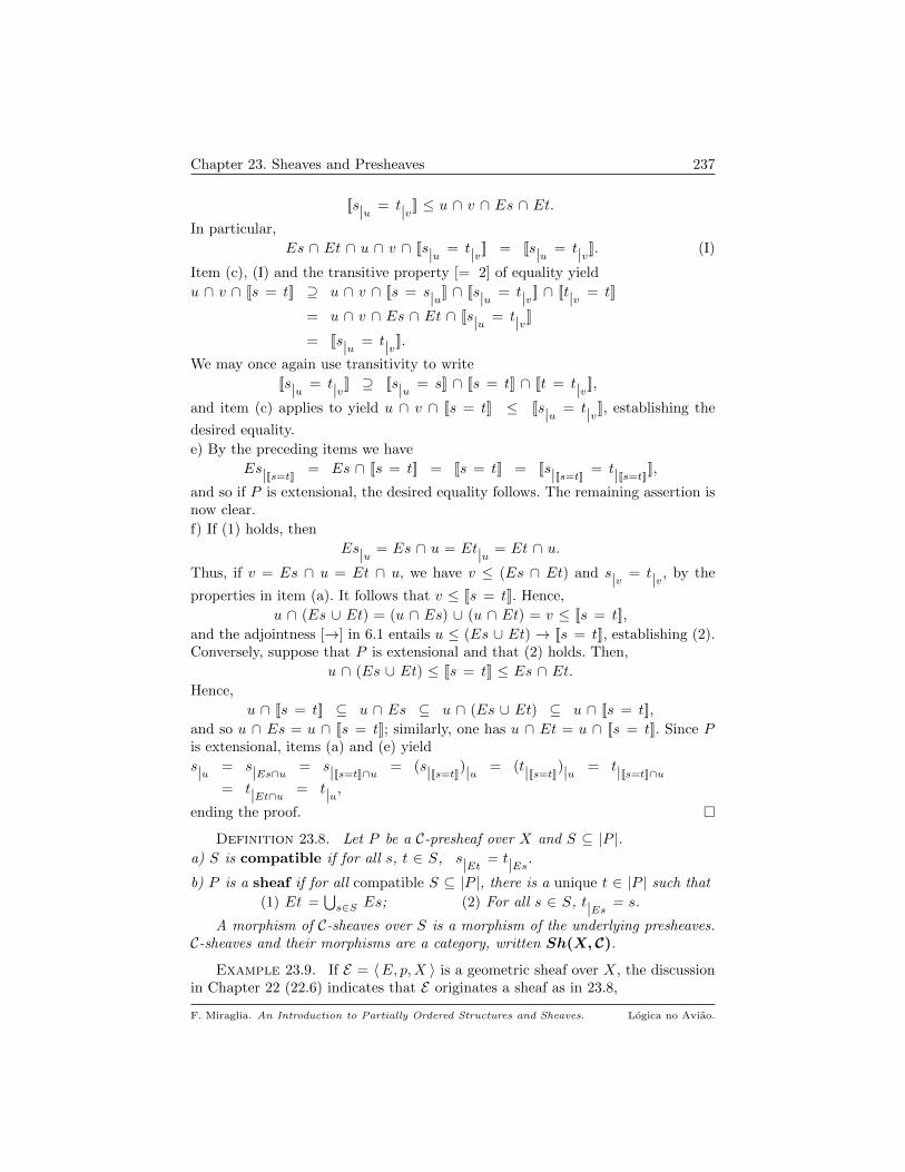
Chapter 23. Sheaves and Presheaves 237
[[s|u = t|v]] ≤ u ∩ v ∩ Es ∩ Et.In particular,
Es ∩ Et ∩ u ∩ v ∩ [[s|u = t|v]] = [[s|u = t|v]]. (I)
Item (c), (I) and the transitive property [= 2] of equality yield
u ∩ v ∩ [[s = t]] ⊇ u ∩ v ∩ [[s = s|u]] ∩ [[s|u = t|v]] ∩ [[t|v = t]]
= u ∩ v ∩ Es ∩ Et ∩ [[s|u = t|v]]= [[s|u = t|v]].
We may once again use transitivity to write
[[s|u = t|v]] ⊇ [[s|u = s]] ∩ [[s = t]] ∩ [[t = t|v]],and item (c) applies to yield u ∩ v ∩ [[s = t]] ≤ [[s|u = t|v]], establishing the
desired equality.
e) By the preceding items we have
Es|[[s=t]] = Es ∩ [[s = t]] = [[s = t]] = [[s|[[s=t]] = t|[[s=t]]]],and so if P is extensional, the desired equality follows. The remaining assertion isnow clear.
f) If (1) holds, then
Es|u = Es ∩ u = Et|u = Et ∩ u.
Thus, if v = Es ∩ u = Et ∩ u, we have v ≤ (Es ∩ Et) and s|v = t|v, by the
properties in item (a). It follows that v ≤ [[s = t]]. Hence,
u ∩ (Es ∪ Et) = (u ∩ Es) ∪ (u ∩ Et) = v ≤ [[s = t]],
and the adjointness [→] in 6.1 entails u ≤ (Es ∪ Et) → [[s = t]], establishing (2).Conversely, suppose that P is extensional and that (2) holds. Then,
u ∩ (Es ∪ Et) ≤ [[s = t]] ≤ Es ∩ Et.Hence,
u ∩ [[s = t]] ⊆ u ∩ Es ⊆ u ∩ (Es ∪ Et) ⊆ u ∩ [[s = t]],
and so u ∩ Es = u ∩ [[s = t]]; similarly, one has u ∩ Et = u ∩ [[s = t]]. Since Pis extensional, items (a) and (e) yield
s|u = s|Es∩u = s|[[s=t]]∩u = (s|[[s=t]])|u = (t|[[s=t]])|u = t|[[s=t]]∩u= t|Et∩u = t|u,
ending the proof.
Definition 23.8. Let P be a C-presheaf over X and S ⊆ |P |.a) S is compatible if for all s, t ∈ S, s|Et = t|Es.b) P is a sheaf if for all compatible S ⊆ |P |, there is a unique t ∈ |P | such that
(1) Et =⋃s∈S Es; (2) For all s ∈ S, t|Es = s.
A morphism of C-sheaves over S is a morphism of the underlying presheaves.C-sheaves and their morphisms are a category, written Sh(X, C).
Example 23.9. If E = 〈E, p,X 〉 is a geometric sheaf over X, the discussionin Chapter 22 (22.6) indicates that E originates a sheaf as in 23.8,
F. Miraglia. An Introduction to Partially Ordered Structures and Sheaves. Logica no Aviao.
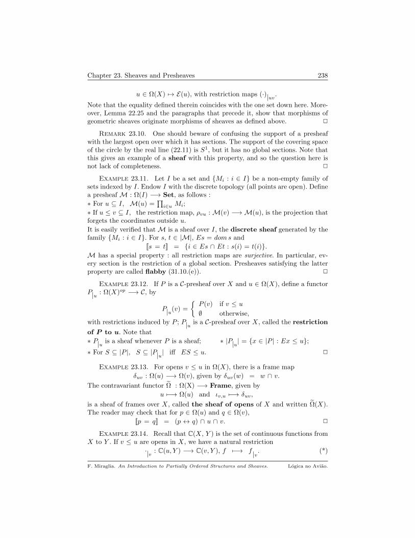
Chapter 23. Sheaves and Presheaves 238
u ∈ Ω(X) 7→ E(u), with restriction maps (·)|uv.Note that the equality defined therein coincides with the one set down here. More-over, Lemma 22.25 and the paragraphs that precede it, show that morphisms ofgeometric sheaves originate morphisms of sheaves as defined above. 2
Remark 23.10. One should beware of confusing the support of a presheafwith the largest open over which it has sections. The support of the covering spaceof the circle by the real line (22.11) is S1, but it has no global sections. Note thatthis gives an example of a sheaf with this property, and so the question here isnot lack of completeness. 2
Example 23.11. Let I be a set and Mi : i ∈ I be a non-empty family ofsets indexed by I. Endow I with the discrete topology (all points are open). Definea presheaf M : Ω(I) −→ Set, as follows :
∗ For u ⊆ I, M(u) =∏i∈u Mi;
∗ If u ≤ v ⊆ I, the restriction map, ρvu :M(v) −→M(u), is the projection thatforgets the coordinates outside u.
It is easily verified thatM is a sheaf over I, the discrete sheaf generated by thefamily Mi : i ∈ I. For s, t ∈ |M|, Es = doms and
[[s = t]] = i ∈ Es ∩ Et : s(i) = t(i).M has a special property : all restriction maps are surjective. In particular, ev-ery section is the restriction of a global section. Presheaves satisfying the latterproperty are called flabby (31.10.(e)). 2
Example 23.12. If P is a C-presheaf over X and u ∈ Ω(X), define a functorP|u : Ω(X)op −→ C, by
P|u(v) =
P (v) if v ≤ u
∅ otherwise,
with restrictions induced by P ; P|u is a C-presheaf over X, called the restriction
of P to u. Note that
∗ P|u is a sheaf whenever P is a sheaf; ∗ |P|u| = x ∈ |P | : Ex ≤ u;∗ For S ⊆ |P |, S ⊆ |P|u| iff ES ≤ u. 2
Example 23.13. For opens v ≤ u in Ω(X), there is a frame map
δuv : Ω(u) −→ Ω(v), given by δuv(w) = w ∩ v.
The contravariant functor Ω : Ω(X) −→ Frame, given by
u 7−→ Ω(u) and ιv,u 7−→ δuv,
is a sheaf of frames over X, called the sheaf of opens of X and written Ω(X).The reader may check that for p ∈ Ω(u) and q ∈ Ω(v),
[[p = q]] = (p ↔ q) ∩ u ∩ v. 2
Example 23.14. Recall that C(X, Y ) is the set of continuous functions fromX to Y . If v ≤ u are opens in X, we have a natural restriction
·|v : C(u, Y ) −→ C(v, Y ), f 7−→ f |v. (*)
F. Miraglia. An Introduction to Partially Ordered Structures and Sheaves. Logica no Aviao.
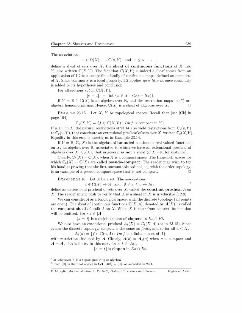
Chapter 23. Sheaves and Presheaves 239
The associations
u ∈ Ω(X) 7−→ C(u, Y ) and v ≤ u 7−→ ·|v,define a sheaf of sets over X, the sheaf of continuous functions of X intoY , also written C(X,Y ). The fact that C(X,Y ) is indeed a sheaf comes from anapplication of 1.2 to a compatible family of continuous maps, defined on open setsof X. Since continuity is a local property, 1.2 applies ipsis litteris, once continuityis added to its hypotheses and conclusion.
For all sections s, t in C(X,Y ),
[[s = t]] = int x ∈ X : s(x) = t(x).If Y = R 4, C(X) is an algebra over R, and the restriction maps in (*) are
algebra homomorphisms. Hence, C(X) is a sheaf of algebras over X. 2
Example 23.15. Let X, Y be topological spaces. Recall that (see [Cb] inpage 194)
Cb(X,Y ) = f ∈ C(X,Y ) : Imf is compact in Y .If u ≤ v in X, the natural restrictions of 23.14 also yield restrictions from Cb(v, Y )to Cb(u, Y ), that constitute an extensional presheaf of sets overX, written Cb(X,Y ).Equality in this case is exactly as in Example 23.14.
If Y = R, Cb(X) is the algebra of bounded continuous real valued functionson X, an algebra over R, associated to which we have an extensional presheaf ofalgebras over X, Cb(X), that in general is not a sheaf (if X =R, for instance).
Clearly, Cb(X) = C(X), when X is a compact space. The Hausdorff spaces forwhich Cb(X) = C(X) are called pseudo-compact. The reader may wish to tryhis hand at proving that the first uncountable ordinal, ω1, with the order topology,is an example of a pseudo compact space that is not compact. 2
Example 23.16. Let A be a set. The associations
u ∈ Ω(X) 7→ A and ∅ 6= v ≤ u 7→ IdA5
define an extensional presheaf of sets over X, called the constant presheaf A onX. The reader might wish to verify that A is a sheaf iff X is irreducible (12.8).
We can consider A as a topological space, with the discrete topology (all pointsare open). The sheaf of continuous functions C(X,A), denoted by A(X), is calledthe constant sheaf of stalk A on X. When X is clear from context, its mentionwill be omitted. For s, t ∈ |A|,
[[s = t]] is a disjoint union of clopens in Es ∩ Et.We also have an extensional presheaf Ab(X) = Cb(X,A) (as in 23.15). Since
A has the discrete topology, compact is the same as finite, and so for all u ≤ X,
Ab(u) = f ∈ C(u,A) : Imf is a finite subset of A,with restrictions induced by A. Clearly, A(u) = Ab(u) when u is compact andA = Ab if A is finite. In this case, for s, t ∈ |Ab|,
[[s = t]] is clopen in Es ∩ Et.
4Or whenever Y is a topological ring or algebra5Since 0 is the final object in Set, A(∅) = 0, as accorded in 23.4.
F. Miraglia. An Introduction to Partially Ordered Structures and Sheaves. Logica no Aviao.
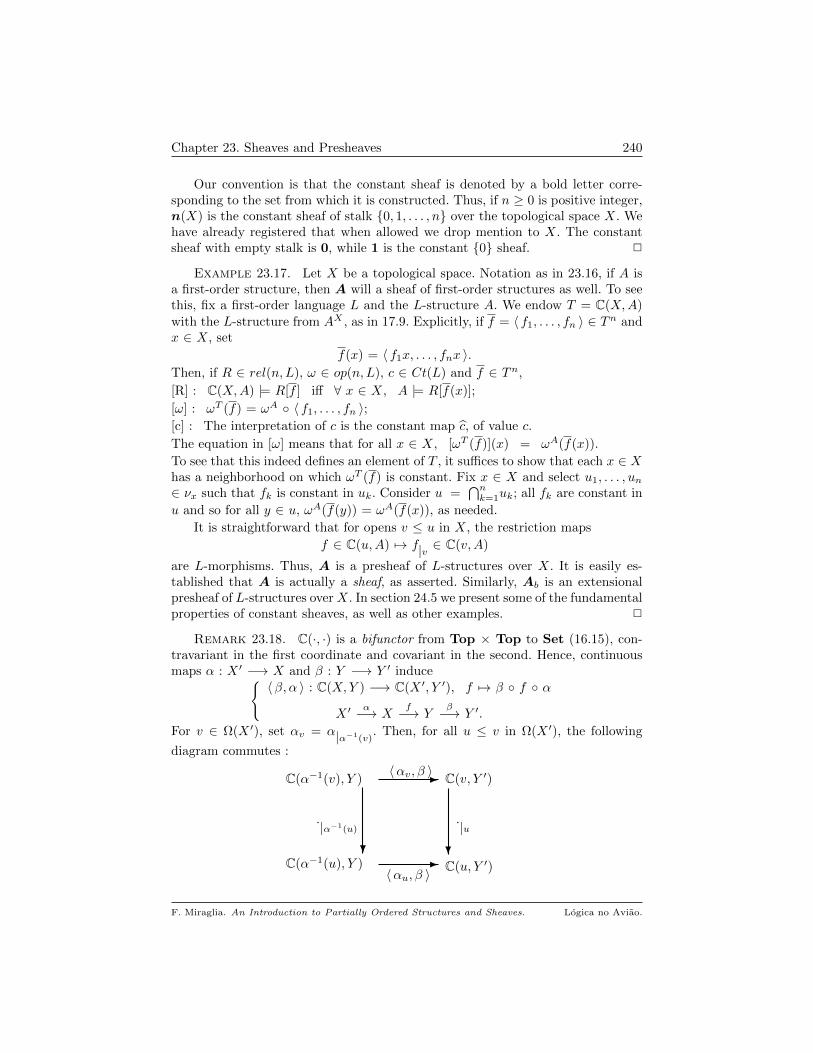
Chapter 23. Sheaves and Presheaves 240
Our convention is that the constant sheaf is denoted by a bold letter corre-sponding to the set from which it is constructed. Thus, if n ≥ 0 is positive integer,n(X) is the constant sheaf of stalk 0, 1, . . . , n over the topological space X. Wehave already registered that when allowed we drop mention to X. The constantsheaf with empty stalk is 0, while 1 is the constant 0 sheaf. 2
Example 23.17. Let X be a topological space. Notation as in 23.16, if A isa first-order structure, then A will a sheaf of first-order structures as well. To seethis, fix a first-order language L and the L-structure A. We endow T = C(X,A)with the L-structure from AX , as in 17.9. Explicitly, if f = 〈 f1, . . . , fn 〉 ∈ Tn andx ∈ X, set
f(x) = 〈 f1x, . . . , fnx 〉.Then, if R ∈ rel(n,L), ω ∈ op(n,L), c ∈ Ct(L) and f ∈ Tn,
[R] : C(X,A) |= R[f ] iff ∀ x ∈ X, A |= R[f(x)];
[ω] : ωT (f) = ωA 〈 f1, . . . , fn 〉;[c] : The interpretation of c is the constant map c, of value c.
The equation in [ω] means that for all x ∈ X, [ωT (f)](x) = ωA(f(x)).
To see that this indeed defines an element of T , it suffices to show that each x ∈ Xhas a neighborhood on which ωT (f) is constant. Fix x ∈ X and select u1, . . . , un∈ νx such that fk is constant in uk. Consider u =
⋂nk=1uk; all fk are constant in
u and so for all y ∈ u, ωA(f(y)) = ωA(f(x)), as needed.
It is straightforward that for opens v ≤ u in X, the restriction maps
f ∈ C(u,A) 7→ f|v ∈ C(v,A)
are L-morphisms. Thus, A is a presheaf of L-structures over X. It is easily es-tablished that A is actually a sheaf, as asserted. Similarly, Ab is an extensionalpresheaf of L-structures overX. In section 24.5 we present some of the fundamentalproperties of constant sheaves, as well as other examples. 2
Remark 23.18. C(·, ·) is a bifunctor from Top × Top to Set (16.15), con-travariant in the first coordinate and covariant in the second. Hence, continuousmaps α : X ′ −→ X and β : Y −→ Y ′ induce
〈β, α 〉 : C(X,Y ) −→ C(X ′, Y ′), f 7→ β f α
X ′α−→ X
f−→ Yβ−→ Y ′.
For v ∈ Ω(X ′), set αv = α|α−1(v). Then, for all u ≤ v in Ω(X ′), the following
diagram commutes :
C(α−1(u), Y )
C(α−1(v), Y )
?
- C(v, Y ′)
·|α−1(u)
〈αv, β 〉
C(u, Y ′)
·|u
〈αu, β 〉
?-
F. Miraglia. An Introduction to Partially Ordered Structures and Sheaves. Logica no Aviao.

Chapter 23. Sheaves and Presheaves 241
This example, as well as 20.9, show that it is important to study morphisms betweensheaves with different bases, giving an indication on how to define such a concept(see Definitions 29.1 and 29.3). 2
Let η : P −→ Q be a morphism of C-presheaves (23.2). We can view η as amap from |P | to |Q|, as follows :
For s ∈ |P |, set ηs = ηEs(s).
The following Lemma summarizes the relations between the “natural transforma-tion” concept of morphism and that just introduced.
Lemma 23.19. Let P and Q be C-presheaves over X. Consider the followingconditions :
(1) There is a unique C-presheaf morphism, η : P −→ Q, such that ηEs(s) = f(s),s ∈ |P |.
(2) For all s ∈ |P | and u ∈ Ω(X),
(i) EQf(s) = EP s;
(ii) f(s|u) = f(s)|u.
(3) For all s, t ∈ |P |,
[mor 1] : EQf(s) = EP s;
[mor 2] : [[s = t]]P ⊆ [[f(s) = f(t)]]Q.
Then,
a) (1) ⇒ (2) ⇒ (3).
b) If Q is extensional, then (3) ⇒ (2).
c) If P and Q are presheaves of sets then (3) and (1) are equivalent. If Q isextensional, all three conditions are equivalent.
Proof. We write E(·) for the extension of sections in P and in Q, the contextmaking it clear to which presheaf the section belongs.
a) (1) ⇒ (2) is an immediate consequence of the definitions.
(2) ⇒ (3) : Clearly it suffices to prove [mor 2]. For s, t ∈ |P |, the properties of
restriction in 23.7.(a) and (2).(ii) yield
(*) [[f(s|[[s=t]]) = f(t|[[s=t]])]] = [[f(s)|[[s=t]] = f(t)|[[s=t]]]]= [[f(s) = f(t)]] ∩ [[s = t]].
On the other hand, s|[[s=t]] = t|[[s=t]] and Es|[[s=t]] = [[s = t]]. Thus, from (2).(i)
and (*) comes
[[s = t]] = [[f(s) = f(t)]] ∩ [[s = t]],
which is equivalent to [mor 2].
b) If 〈 s, v 〉 ∈ P (u) × Ω(u), then
Ef(s|v) = Es|v = Es ∩ v = Ef(s) ∩ v = E(fs)|v. (A)
Thus, [mor 2] and [rest 3] in 23.7.(a) yield
[[f(s|v) = (fs)|v]]] = [[f(s|v) = fs]] ∩ v ⊇ [[s|v = s]] ∩ v = Es ∩ v.
By (A), [[f(s|v) = (fs)|v]] ⊆ Es ∩ v, and so
F. Miraglia. An Introduction to Partially Ordered Structures and Sheaves. Logica no Aviao.
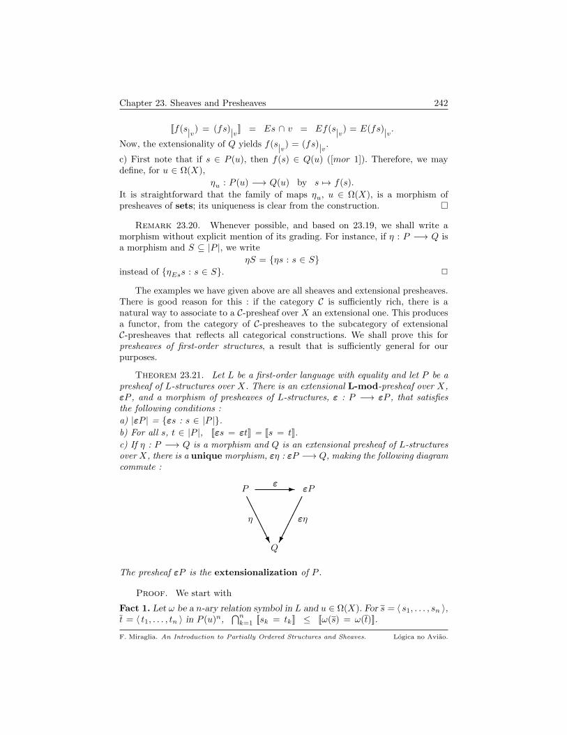
Chapter 23. Sheaves and Presheaves 242
[[f(s|v) = (fs)|v]] = Es ∩ v = Ef(s|v) = E(fs)|v.Now, the extensionality of Q yields f(s|v) = (fs)|v.c) First note that if s ∈ P (u), then f(s) ∈ Q(u) ([mor 1]). Therefore, we maydefine, for u ∈ Ω(X),
ηu : P (u) −→ Q(u) by s 7→ f(s).
It is straightforward that the family of maps ηu, u ∈ Ω(X), is a morphism ofpresheaves of sets; its uniqueness is clear from the construction.
Remark 23.20. Whenever possible, and based on 23.19, we shall write amorphism without explicit mention of its grading. For instance, if η : P −→ Q isa morphism and S ⊆ |P |, we write
ηS = ηs : s ∈ Sinstead of ηEss : s ∈ S. 2
The examples we have given above are all sheaves and extensional presheaves.There is good reason for this : if the category C is sufficiently rich, there is anatural way to associate to a C-presheaf over X an extensional one. This producesa functor, from the category of C-presheaves to the subcategory of extensionalC-presheaves that reflects all categorical constructions. We shall prove this forpresheaves of first-order structures, a result that is sufficiently general for ourpurposes.
Theorem 23.21. Let L be a first-order language with equality and let P be apresheaf of L-structures over X. There is an extensional L-mod-presheaf over X,εP , and a morphism of presheaves of L-structures, ε : P −→ εP , that satisfiesthe following conditions :
a) |εP | = εs : s ∈ |P |.b) For all s, t ∈ |P |, [[εs = εt]] = [[s = t]].
c) If η : P −→ Q is a morphism and Q is an extensional presheaf of L-structuresover X, there is a unique morphism, εη : εP −→ Q, making the following diagramcommute :
P - εP
η εη
Q
ε
AAAAAU
The presheaf εP is the extensionalization of P .
Proof. We start with
Fact 1. Let ω be a n-ary relation symbol in L and u ∈ Ω(X). For s = 〈 s1, . . . , sn 〉,t = 〈 t1, . . . , tn 〉 in P (u)n,
⋂nk=1 [[sk = tk]] ≤ [[ω(s) = ω(t)]].
F. Miraglia. An Introduction to Partially Ordered Structures and Sheaves. Logica no Aviao.

Chapter 23. Sheaves and Presheaves 243
Proof. 6 Let u1, . . . , un ∈ Ω(X) be such that for 1 ≤ k ≤ n,
uk ≤ (Esk ∩ Etk) and sk|uk = tk|uk ,
and set u =⋂nk=1 uk. It follows from [rest 3] in 23.7.(a) that
For all 1 ≤ k ≤ n, sk|u = tk|u. (I)
Since P is a presheaf of L-structures, the restriction maps are L-morphisms, thatis,
ω(s)|u = ω(s1|u, . . . , sn|u). (II)
(I) and (II) yield ω(s)|u = ω(t)|u, showing that u ⊆ [[ω(s) = ω(t)]]. Since
Ω(X) is a [∧,∨
]-lattice, 8.4 guarantees that⋂nk=1 [[sk = tk]] =
⋃⋂nk=1 uk : uk ≤ Esk ∩Etk and sk|uk = tk|uk,
and the inequality in the statement follows.
For s, t ∈ |P | define
s θ t iff Es = Et = [[s = t]].
It is clear that θ is an equivalence relation on |P |.Fact 2. For u ∈ Ω(X), set θu = θ ∩ (P (u) × P (u)). Then, θu is a congruenceon the L-structure P (u).
Proof. Clearly, θu is an equivalence relation on P (u). Let ω be a n-ary operationsymbol in L. It must be shown that for s = 〈 s1, . . . , sn 〉 and t = 〈 t1, . . . , tn 〉 inP (u)n, we have
sk θu tk, for 1 ≤ k ≤ n ⇒ ω(s) θu ω(t). (III)
It is clear that Eω(s) = Eω(t) = u, because ω is an operation on P (u). From thehypothesis in (III) and Fact 1, we obtain⋃n
k=1 [[sk = tk]] =⋃nk=1 Esk = u ≤ [[ω(s) = ω(t)]],
and so [E =] in 23.7.(b) entails [[ω(s) = ω(t)]] = u, ending the proof of Fact 2.
For u ∈ Ω(X), let
εP (u) = P (u)/θu,
be the quotient L-structure of P (u) by θu, as in 17.21; write
εu : P (u) −→ P (u)/θufor the canonical quotient L-morphism. For s ∈ |P |, write εs =def s/θEs. Foropens u ≤ v in X, define
ρvu : εP (v) −→ εP (u), by ρvu(εs) = ε(s|u).
Fact 3. For opens u ≤ v in X, ρvu is a L-morphism such that
(1) If u ≤ v ≤ w are opens in X, ρwu = ρvu ρwv;(2) ρuu = IdεP (u).
Moreover, εP : Ω(X) −→ L-mod defined by
u 7−→ P (u) and ιuv 7−→ ρvuis a presheaf over X.
Proof. Fix opens u ≤ v in X and let f = εu (·)|u.
6In fact, we should use ωP (u), but this would overload notation.
F. Miraglia. An Introduction to Partially Ordered Structures and Sheaves. Logica no Aviao.

Chapter 23. Sheaves and Presheaves 244
P (v)(·)|u−→ P (u)
εu−→ εP (u).
By construction, f is a L-morphism. We now verify that
θv ⊆ θf = 〈 s, t 〉 ∈ P (v)2 : fs = ft,that is, for all s, t ∈ P (v), s θv t ⇒ s|u θu t|u. Since u = Es = Et = [[s = t]],
23.7.(d) yields
[[s|u = t|u]] = u ∩ [[s = t]] = u
and the conclusion follows from [rest 2] in 23.7.(a). By the universal property in
17.21, there is a unique L-morphism, f : εP (v) −→ εP (u), such that
f εv = f = εu (·)|u.
Since f is pointwise identical with ρvu, the latter is a L-morphism, as desired. Theverification of conditions (1) and (2) is straightforward and εP is a presheaf ofL-structures over X.
Fact 4. For all s, t ∈ |P |,(1) Eεs = Es;
(2) [[εs = εt]] = [[s = t]];
(3) εP is an extensional presheaf of L-structures over X.
Proof. (1) is clear, because if s ∈ P (u), then εs ∈ εP (u). For (2), if u ≤ Es ∩ Etis such that s|u = t|u, then
ρEs,u(εs) = ε(s|u) = ε(t|u) = ρEt,u(εt),
and u ≤ [[εs = εt]]. Hence, [[s = t]] ⊆ [[εs = εt]]. Conversely, if v ≤ Es ∩ Et,satisfies ρEs,v(εs) = ρEt,v(εt), the definition of the restriction maps ρ∗∗ entails
ε(s|v) = ε(t|v),that is, s|v θv t|v. Hence, items (a) and (d) in 23.7 yield
v ∩ Es = Es|v = Et|v = v ∩ Et = [[s|v = t|v]] = v ∩ [[s = t]].
Since v ≤ Es ∩ Et, the preceding equations entail v = v ∩ [[s = t]], that is,v ≤ [[s = t]]. It follows that [[εs = εt]] ⊆ [[s = t]], completing the verification of(2). Item (3) is immediate from (1) and (2).
Up to now we have proven (a) and (b) (Fact 3.(2)) in the statement of theTheorem. It remains to verify (c).
If η = ηu ∈ [P (u), Q(u)] : u ∈ Ω(X) is a natural transformation from Pto Q (23.2), define εη : εP −→ Q as follows :
For u ∈ Ω(X), (εη)u : εP (u) −→ Q(u) is given by
(εη)u(εs) = ηus.
To see that this well defined, let Es = Et = [[s = t]], s, t ∈ P (u). By Lemma23.19, we have
[[s = t]] ⊆ [[ηus = ηut]],
F. Miraglia. An Introduction to Partially Ordered Structures and Sheaves. Logica no Aviao.
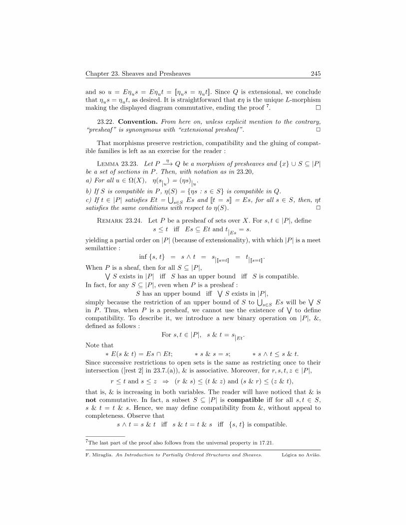
Chapter 23. Sheaves and Presheaves 245
and so u = Eηus = Eηut = [[ηus = ηut]]. Since Q is extensional, we concludethat ηus = ηut, as desired. It is straightforward that εη is the unique L-morphismmaking the displayed diagram commutative, ending the proof 7.
23.22. Convention. From here on, unless explicit mention to the contrary,“presheaf” is synonymous with “extensional presheaf”. 2
That morphisms preserve restriction, compatibility and the gluing of compat-ible families is left as an exercise for the reader :
Lemma 23.23. Let Pη−→ Q be a morphism of presheaves and x ∪ S ⊆ |P |
be a set of sections in P . Then, with notation as in 23.20,
a) For all u ∈ Ω(X), η(s|u) = (ηs)|u.
b) If S is compatible in P , η(S) = ηs : s ∈ S is compatible in Q.
c) If t ∈ |P | satisfies Et =⋃s∈S Es and [[t = s]] = Es, for all s ∈ S, then, ηt
satisfies the same conditions with respect to η(S). 2
Remark 23.24. Let P be a presheaf of sets over X. For s, t ∈ |P |, define
s ≤ t iff Es ⊆ Et and t|Es = s.
yielding a partial order on |P | (because of extensionality), with which |P | is a meetsemilattice :
inf s, t = s ∧ t = s|[[s=t]] = t|[[s=t]].When P is a sheaf, then for all S ⊆ |P |,∨
S exists in |P | iff S has an upper bound iff S is compatible.
In fact, for any S ⊆ |P |, even when P is a presheaf :
S has an upper bound iff∨S exists in |P |,
simply because the restriction of an upper bound of S to⋃s∈S Es will be
∨S
in P . Thus, when P is a presheaf, we cannot use the existence of∨
to definecompatibility. To describe it, we introduce a new binary operation on |P |, &,defined as follows :
For s, t ∈ |P |, s & t = s|Et.Note that
∗ E(s & t) = Es ∩ Et; ∗ s & s = s; ∗ s ∧ t ≤ s & t.
Since successive restrictions to open sets is the same as restricting once to theirintersection ([rest 2] in 23.7.(a)), & is associative. Moreover, for r, s, t, z ∈ |P |,
r ≤ t and s ≤ z ⇒ (r & s) ≤ (t & z) and (s & r) ≤ (z & t),
that is, & is increasing in both variables. The reader will have noticed that & isnot commutative. In fact, a subset S ⊆ |P | is compatible iff for all s, t ∈ S,s & t = t & s. Hence, we may define compatibility from &, without appeal tocompleteness. Observe that
s ∧ t = s & t iff s & t = t & s iff s, t is compatible.
7The last part of the proof also follows from the universal property in 17.21.
F. Miraglia. An Introduction to Partially Ordered Structures and Sheaves. Logica no Aviao.
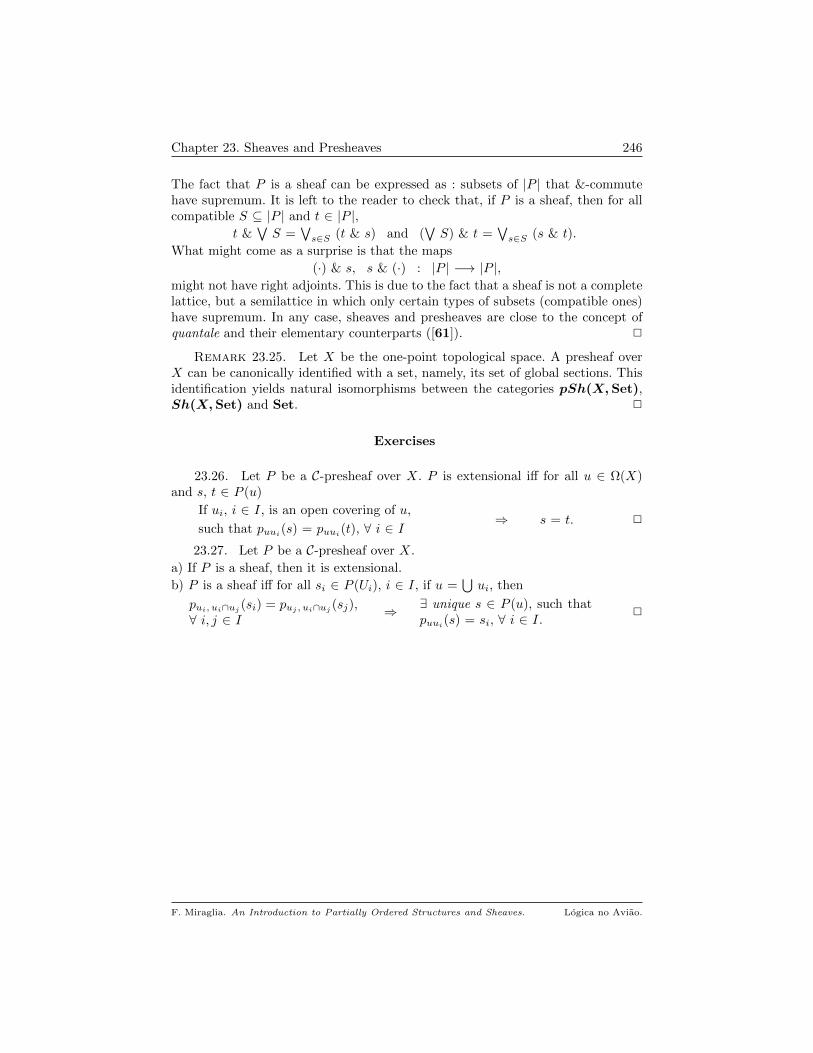
Chapter 23. Sheaves and Presheaves 246
The fact that P is a sheaf can be expressed as : subsets of |P | that &-commutehave supremum. It is left to the reader to check that, if P is a sheaf, then for allcompatible S ⊆ |P | and t ∈ |P |,
t &∨S =
∨s∈S (t & s) and (
∨S) & t =
∨s∈S (s & t).
What might come as a surprise is that the maps
(·) & s, s & (·) : |P | −→ |P |,might not have right adjoints. This is due to the fact that a sheaf is not a completelattice, but a semilattice in which only certain types of subsets (compatible ones)have supremum. In any case, sheaves and presheaves are close to the concept ofquantale and their elementary counterparts ([61]). 2
Remark 23.25. Let X be the one-point topological space. A presheaf overX can be canonically identified with a set, namely, its set of global sections. Thisidentification yields natural isomorphisms between the categories pSh(X,Set),Sh(X,Set) and Set. 2
Exercises
23.26. Let P be a C-presheaf over X. P is extensional iff for all u ∈ Ω(X)and s, t ∈ P (u)
If ui, i ∈ I, is an open covering of u,
such that puui(s) = puui(t), ∀ i ∈ I⇒ s = t. 2
23.27. Let P be a C-presheaf over X.
a) If P is a sheaf, then it is extensional.
b) P is a sheaf iff for all si ∈ P (Ui), i ∈ I, if u =⋃ui, then
pui, ui∩uj (si) = puj , ui∩uj (sj),∀ i, j ∈ I ⇒ ∃ unique s ∈ P (u), such that
puui(s) = si, ∀ i ∈ I.2
F. Miraglia. An Introduction to Partially Ordered Structures and Sheaves. Logica no Aviao.

CHAPTER 24
Presheaves of Sets
In this chapter we discuss sheaves and presheaves of sets. The reasons for thisare twofold :
∗ Without a doubt, presheaves of sets underlie very important mathematical con-structions and are frequently used as an introduction to the subject;
∗ Since we are ultimately interested in First-Order Logic, presheaves of first-order structures are our main concern. Consider how the classical concept of L-structure is defined. The basic building blocks are sets and constructions with sets.Thus, a L-structure is a set, together with maps, elements and certain distinguishedsubsets of its finite powers. It seems, reasonable to proceed by analogy to arrive atthe notion of L-structures in presheaves, replacing the category of sets by that ofpresheaves. If this path is taken, elementary “set theory” must be internalized inthe category of presheaves, that is, one has to establish the analogues of unions,intersections, the power set, maps, elements and relations, among other things.
It will turn out that “L-structure in the category of presheaves” comes to thesame thing as “presheaves of L-structures”, but the conceptual role of workinginside the category of presheaves over a topological space is important to under-stand other situations, in which such a correspondence is false, as is the case inthe general framework of Topoi, originating with A. Grothendieck and his school,to treat Algebraic Geometry, just to mention one notable example.
Throughout this Chapter, X is a topological space and Ω = Ω(X) is the frameof opens in X. All presheaves will be extensional. Write pSh(X) and Sh(X) forthe categories of presheaves and sheaves of sets over X, respectively.
We employ Proposition 23.7 and Lemma 23.19, without necessarily mentioningit. The definition of extensionality, [ext], appears in 23.6.(c).
1. Categorical Constructions
This section is dedicated to the description of some of the basic categoricalconstructions in pSh(X) and Sh(X).
24.1. Initial and Final Objects. These are the constant sheaves 0 and 1,respectively (see 23.16). It is clear that for each presheaf P on X, there are uniquemorphisms from 0 to P and from P to 1 1. 2
1The empty map is the unique map with empty domain, into any set.
247
Chapter 24. Presheaves of Sets 248
24.2. Products. Let Pi, i ∈ I, be a family of presheaves overX. For u ∈ Ω(X),define
(∏i∈I Pi)(u) =
∏i∈I Pi(u),
and for an open subset v of u, a restriction
(∏i∈I Pi)(u) −→ (
∏i∈I Pi)(v), 〈 si 〉 7→ 〈 si|v 〉
It is straightforward that this defines a presheaf over X, which is a sheaf if thesame is true of each component. The canonical projections
πiu : (∏i∈I Pi)(u) −→ Pi(u),
are presheaf morphisms, πi : (∏i∈I Pi) −→ Pi. The pair
〈∏i∈I Pi, πii∈I 〉
is the product of the family Pi in the categories pSh(X) or Sh(X).
Write P =∏i∈I Pi; the domain of P is given by
|P | = 〈 si 〉 ∈∏i∈I |Pi| : ∀ i, j ∈ I, Esi = Esj.
Note the distinction between |P | and the product of the |Pi| : only i-tuples withconstant extent are in |P |. If s = 〈 si 〉, t = 〈 ti 〉 are sections in |P |, then 2
[[s = t]] =∧i∈I [[si = ti]] = int
(⋂i∈I [[si = ti]]
).
In particular, Es =∧i∈I Esi = Esi, for any i ∈ I. The projections πi may
be written as maps, πi : |P | −→ |Pi|, πis = si. If s, t are sections in P , then
Es = Et = [[s = t]],
implies that for all i ∈ I,
Esi = Eti = [[si = ti]]
and the extensionality of each component entails s = t. Hence, P is an extensionalpresheaf. When I = ∅, we have
P ∅ =def P0 = 1,
where 1 is the constant sheaf 0, as in 23.16. The reason for this is that in anycategory, the empty product is its final object. In particular, in Set, the emptyproduct is the final object 1 = 0. 2
24.3. Fibered product over a map. Let λ : P −→ Q be a morphism ofpresheaves over X. Define, for u ∈ Ω(X),
(P ×λ P )(u) = 〈 s, t 〉 ∈ P (u) × P (u) : λu(s) = λu(t),with restrictions induced by the product P × P . P ×λ P is a presheaf, called thefibered product of P over λ. If P is a sheaf, the same is true of P ×λ P . Thereare morphisms,
δ1, δ2 : P ×λ P −→ P ,
given by the restriction to (P ×λ P )(u) ⊆ P (u) × P (u), of the projections ofthe product presheaf P × P on each coordinate. Clearly, λ δ1 = λ δ2.
If λ = IdP , the fibered product of P over λ is the graph of the identity relationon P , ∆P ; when P is clear from context, write ∆ for this presheaf. 2
24.4. Equalizers. Let λ, β be morphisms from P to Q. For each u ∈ Ω(X),define
2Recall that∧
in the frame Ω(X) is the interior of the intersection; 2.11.(b).
F. Miraglia. An Introduction to Partially Ordered Structures and Sheaves. Logica no Aviao.
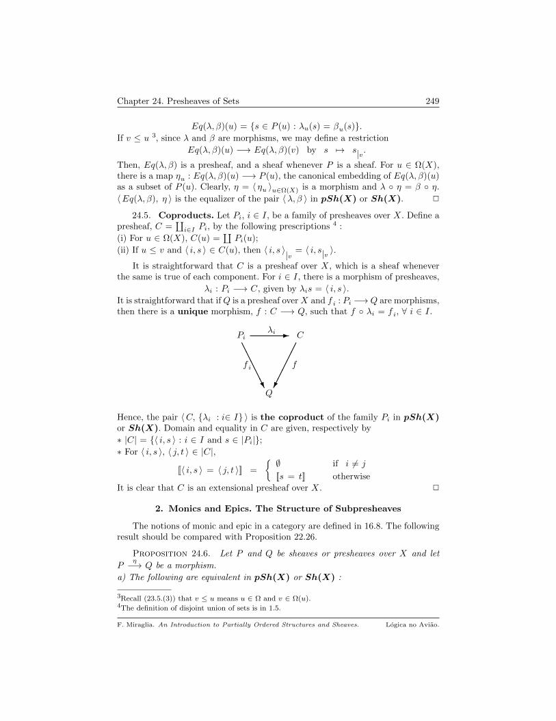
Chapter 24. Presheaves of Sets 249
Eq(λ, β)(u) = s ∈ P (u) : λu(s) = βu(s).If v ≤ u 3, since λ and β are morphisms, we may define a restriction
Eq(λ, β)(u) −→ Eq(λ, β)(v) by s 7→ s|v.Then, Eq(λ, β) is a presheaf, and a sheaf whenever P is a sheaf. For u ∈ Ω(X),there is a map ηu : Eq(λ, β)(u) −→ P (u), the canonical embedding of Eq(λ, β)(u)as a subset of P (u). Clearly, η = 〈 ηu 〉u∈Ω(X) is a morphism and λ η = β η.
〈Eq(λ, β), η 〉 is the equalizer of the pair 〈λ, β 〉 in pSh(X) or Sh(X). 2
24.5. Coproducts. Let Pi, i ∈ I, be a family of presheaves over X. Define apresheaf, C =
∐i∈I Pi, by the following prescriptions 4 :
(i) For u ∈ Ω(X), C(u) =∐Pi(u);
(ii) If u ≤ v and 〈 i, s 〉 ∈ C(u), then 〈 i, s 〉|v = 〈 i, s|v 〉.
It is straightforward that C is a presheaf over X, which is a sheaf wheneverthe same is true of each component. For i ∈ I, there is a morphism of presheaves,
λi : Pi −→ C, given by λis = 〈 i, s 〉.It is straightforward that if Q is a presheaf over X and f i : Pi −→Q are morphisms,then there is a unique morphism, f : C −→ Q, such that f λi = f i, ∀ i ∈ I.
Pi - C
f i f
Q
λi
AAAAAU
Hence, the pair 〈C, λi : i∈ I 〉 is the coproduct of the family Pi in pSh(X)or Sh(X). Domain and equality in C are given, respectively by
∗ |C| = 〈 i, s 〉 : i ∈ I and s ∈ |Pi|;∗ For 〈 i, s 〉, 〈 j, t 〉 ∈ |C|,
[[〈 i, s 〉 = 〈 j, t 〉]] =
∅ if i 6= j
[[s = t]] otherwise
It is clear that C is an extensional presheaf over X. 2
2. Monics and Epics. The Structure of Subpresheaves
The notions of monic and epic in a category are defined in 16.8. The followingresult should be compared with Proposition 22.26.
Proposition 24.6. Let P and Q be sheaves or presheaves over X and let
Pη−→ Q be a morphism.
a) The following are equivalent in pSh(X) or Sh(X) :
3Recall (23.5.(3)) that v ≤ u means u ∈ Ω and v ∈ Ω(u).4The definition of disjoint union of sets is in 1.5.
F. Miraglia. An Introduction to Partially Ordered Structures and Sheaves. Logica no Aviao.

Chapter 24. Presheaves of Sets 250
(1) η is monic; (2) For all u ∈ Ω(X), ηu is injective;
(3) For all s, t ∈ |P |, [[ηs = ηt]] = [[s = t]].
b) The following are equivalent in pSh(X) or Sh(X) :
(1) η is epic.
(2) For all t ∈ |Q|, there are ui ⊆ Ω(X) and si ∈ P (ui), i ∈ I,such that
(i)⋃i∈ I ui = Et; (ii) For all i ∈ I, t|ui = ηui(si).
(3) For all t ∈ |Q|, Et =⋃s∈|P | [[t = s]].
c) The following are equivalent in pSh(X) or Sh(X) :
(1) η is an isomorphism. (2) For all u ∈ Ω(X), ηu is bijective.
Proof. We treat sheaves and presheaves at the same time, asking the readerto notice that, when P and Q are sheaves, the objects we need, fibered productover a morphism (24.3) and the sheaf of opens of X (23.13), are sheaves.
(a) Clearly, (2) ⇒ (1), while (2) ⇒ (1) can be handled exactly as in Proposition22.26, by considering the two maps originating in the fibered product of P over ηwith values in P .
(2) ⇒ (3) : If s, t ∈ |P |, then [[s = t]] ⊆ [[ηs = ηt]] ([mor 2]). To prove the reverse
inclusion, set w = [[ηs = ηt]]]; note that [mor 1] implies w ⊆ Et ∩ Es. Thus, boths|w and t|w are in P (w). Hence,
Eη(s|w) = Es|w = Es ∩ w = w;
similarly, we can show that Eη(t|w) = w. Moreover,
[[η(s|w) = η(t|w)]] = [[(ηs)|w = (ηt)|w]] = [[ηs = ηt]] ∩ w = w.
Thus, [ext] yields η(s|w) = η(t|w) in Q(w). Since ηw is injective, we get s|w = t|w.
Now, [rest 3] entails w = [[[s|w = t|w]] = [[s = t]] ∩ w, and so w ⊆ [[s = t]],
as desired.
(3) ⇒ (2) : Suppose s, t ∈ P (u) satisfy ηs = ηt. Then,
Eηs = Eηt = [[ηs = ηt]].
Hence, Es = Et = [[s = t]], and the conclusion follows by extensionality.
b) It is easily seen that (2) iff (3); we prove (1) ⇒ (2), leaving the converse, as
well as item (c) as exercises. Recall that Ω (23.13) is the sheaf of opens of X. We
define two morphisms, α, β : Q −→ Ω, as follows : for t ∈ Q(u), set
∗ αu(t) = 〈u, u 〉; ∗ βu(t) = 〈⋃s∈|P | [[ηs = t]], u 〉.
Clearly, αu, βu are maps from Q(u) into Ω(u) = 〈 v, u 〉 : v ≤ u. We shall verifythat β is a morphism, omitting the (much simpler) case of α. For t ∈ Q(u) andv ≤ u, it must be shown that
βv(t|v) = βu(t)|v. (I)
It suffices to check that the first coordinate of these pairs are the same in Ω(v),since both second coordinates are v. We have
F. Miraglia. An Introduction to Partially Ordered Structures and Sheaves. Logica no Aviao.
Chapter 24. Presheaves of Sets 251⋃s∈|P | [[ηs = t|v]] =
⋃s∈|P | v ∩ [[ηs = t]]
= v ∩⋃s∈|P | [[ηs = t]].
(II)
Since restriction to v in Ω is given by intersection with v in both coordinates, itis clear that (II) entails (I) and so β is a morphism of presheaves. Note that foru ∈ Ω(X) and s ∈ P (u), βu(ηu(s)) = 〈u, u 〉, because⋃
a∈|P | [[ηa = ηs]] = Eηs = u.
Hence, α η = β η; since η is epic, this entails α = β, completing the proof.
Example 24.7. Important example of sheaves come from the theory of an-alytic functions. For an open set u in complex plane C, let H(u) be the ring ofholomorphic functions in u, with the canonical restriction maps if v ≤ u. If T isan open set in C, let HT be the sheaf of analytic functions in opens of T . There is
a morphism, HTexp−→ HT , given by f 7→ ef . It is clear that exp is monic. The Rie-
mann mapping theorem gives a necessary and sufficient condition for an analyticmap to a have a logarithm : its domain must be simply connected. Since C hasa basis consisting of simply connected opens, 24.6.(b) entails that exp is an epic.However, expu is onto iff u is simply connected. This shows that it is impossible todo better than conditions (2) and (3) in the statement of 24.6, even if dealing withsheaves. Similar examples are obtained from the distinction between exact andclosed differential forms in open sets that are not simply connected. This examplealso shows that a morphism of sheaves may be monic and epic without being anisomorphism. 2
Item (a) in Proposition 24.6.(a) is the basis of the following
Definition 24.8. If P is a presheaf over X, a subpresheaf of P is a presheafQ over X such that for all u ≤ v in Ω(X),
∗ Q(u) ⊆ P (u);
∗ The restriction of Q is that induced by P .
Or equivalently, a subpresheaf Q of P is a subset |Q| ⊆ |P | that is closed underthe restriction map of P .
If P is a sheaf, a subsheaf of P is a subpresheaf Q that has gluing of allcompatible families, i.e., for all compatible S ⊆ |Q|,
∃ ! t in |Q|, such that Et =⋃s∈S Es and t|Es = s, ∀ s ∈ S.
Write Q ⊆ P to indicate that Q is a subpresheaf of P and PP (X) for the set ofsubpresheaves of P .
Remark 24.9. It is clear that 〈 PP (X), ⊆〉 is a partially ordered set. More-over, if S, T ∈ PP (X), then
S ⊆ T iff |S| ⊆ |T |,a fact that will be used repeatedly below without further comment. 2
24.10. Intersections. If Pα, α ∈ A, are subpresheaves of P , set, for u ∈ Ω(X),
[⋂α∈A Pα](u) =
⋂α∈A Pα(u),
With the restriction maps induced by P ,⋂Pα is a subpresheaf of P , the inter-
section of the Pα. Further,⋂Pα is a sheaf, if each Pα is a sheaf.
F. Miraglia. An Introduction to Partially Ordered Structures and Sheaves. Logica no Aviao.
Chapter 24. Presheaves of Sets 252
The presheaf⋂Pα is the meet of the family Pα in the poset PP (X), which
is, therefore, a complete lattice. It is left to reader to describe domain, extent andequality of the intersection of subpresheaves. 2
A description of “unions”, or more precisely of joins, in the complete latticePP (X) is the content of Exercise 24.71.
Now consider the analogous problem for subsheaves. There is no problem withintersection, as noted in 24.10. For joins, it is another story. With notation as in24.71, the point is that there may be many compatible subsets of the union of thePα that have no gluing in it. To treat this problem, we introduce :
Definition 24.11. Let P be a presheaf over X, C,B ⊆ |P | and T a sub-presheaf of P .
a) C is dense in B iff for all b ∈ B, 5 Eb =⋃c∈C [[b = c]], i.e., if for all b ∈ B,
there is an open covering ui of Eb, together with ci ∈ C, such that b|ui = ci|ui ,for all i ∈ I.
b) T is a closed subpresheaf of P , if for all t ∈ |P |,Et =
⋃a∈T [[a = t]] ⇒ t ∈ |T |.
Write PP (X) for the set of closed subpresheaves of P .
c) The subpresheaf generated by B in P is
pB =⋂Q ⊆ P : Q is a presheaf and B ⊆ |Q|.
d) The closed subpresheaf generated by B in P is
B =⋂Q ⊆ P : Q is a closed subpresheaf and B ⊆ |Q|.
B is called the closure of B in P 6.
Clearly, B ⊆ |pB| ⊆ |B| and pB is a subpresheaf of B. Moreover, 〈PP (X), ⊆〉is a poset.
Remark 24.12. If P is a presheaf and S ∪ x ⊆ |P |, then the followingconditions are equivalent :
(1) Ex ≤⋃s∈S [[s = x]]; (2) Ex =
⋃s∈S [[s = x]].
To see this, just recall that [[y = x]] ≤ Ex, for all y ∈ |P |, by [E =] in 23.7.(b).Similarly, if S ⊆ T ⊆ |P |, then (1) entails Ex =
⋃t∈T [[t = x]], because⋃
s∈S [[s = x]] ⊆⋃t∈T [[t = x]].
These relations will be used frequently, without comment. 2
Lemma 24.13. If P is a sheaf over X and Q ⊆ P , then Q is a closed sub-presheaf of P iff Q is a subsheaf of P . In particular, PP (X) is the completelattice of subsheaves of P .
Proof. Suppose that Q is a subsheaf of P and t ∈ |P | verifies Et =⋃q∈|Q| [[q = t]]. Consider the family
S = q|[[q=t]] : q ∈ |Q|.
5Compare with 22.13.(c).6Here there is need of Exercise 24.72.(b).
F. Miraglia. An Introduction to Partially Ordered Structures and Sheaves. Logica no Aviao.

Chapter 24. Presheaves of Sets 253
Since Q is a presheaf, it is closed under restrictions. Hence, S ⊆ |Q|. Next, observethat S is compatible, because for all q ∈ |Q|
q|[[q=t]] = t|[[q=t]],by 23.7.(e). Alternatively, since Eq|[[q=t]] = [[q = t]], for q, q′ ∈ |Q|,(q|[[q=t]])|[[q′=t]] = (t|[[q=t]])|[[q′=t]] = t|[[q=t]]∩[[q′=t]]
= (t|[[q′=t]])|[[q=t]]= (q′|[[q′=t]])|[[[q=t]],
verifying the compatibility of S. Since Q is a sheaf, there is s ∈ |Q| such that
Es =⋃q∈|Q| [[q = t]] and s|[[q=t]] = q|[[q=t]] = t|[[q=t]].
Hence, Es = Et and the transitive property of equality ([= 2] in 23.7.(b)) entailsthat for all q ∈ |Q|,[[s = t]] ⊇ [[s = t|[[q=t]]]] ∩ [[t|[[q=t]] = t]] = [[s = t|[[q=t]]]] ∩ [[q = t]]
= [[s|[[q=t]] = t|[[q=t]]]] = [[q = t]].
Thus, [[s = t]] ⊇⋃q∈|Q| [[q = t]] = Es = Et, and extensionality guarantees
that s = t ∈ |Q|, as desired.
Conversely, suppose that Q is a closed subpresheaf of P and that S ⊆ |Q| iscompatible. Then, S has a gluing t in |P | (it is a sheaf). Conditions (1) and (2)in 23.8.(b) yield
(1) Et =⋃s∈S Es; (2) t|Es = s, ∀ s ∈ S.
But then,⋃s∈S [[s = t]] =
⋃s∈S [[t|Es = t]] =
⋃s∈S Es ∩ [[t = t]]
= Et ∩⋃s∈S Es = Et ∩ Et = Et,
and so we must have (24.12) Et =⋃q∈|Q| [[q = t]]. Since Q is a closed subpresheaf
of P , we obtain t ∈ Q, as needed.
Lemma 24.14. Let µ, η : P −→ Q be presheaf morphisms and let D be adense subset of sections in P . The following are equivalent :
(1) µ = η; (2) µ|D = η|D.
Proof. We prove that (2) ⇒ (1). For s ∈ |P | we may write
Es =⋃d∈D [[s = d]]. (I)
The transitive law for equality, [mor 1] and [mor 2] in 23.7.(3) yield, for d ∈ D,
[[µs = ηs]] ⊇ [[µs = µd]] ∩ [[µd = ηd]] ∩ [[ηd = ηs]]
= [[µs = µd]] ∩ Ed ∩ [[ηd = ηs]]
⊇ [[s = d]] ∩ [[s = d]] = [[s = d]],
and so, taking joins with respect to d ∈ D, (I) entails
Es = Eµs = Eηs = [[µs = ηs]],
and extensionality implies µs = ηs, as desired.
Theorem 24.15. Let P be a presheaf over X and Γ ⊆ |P |. For u ∈ Ω(X),set Γ(u) = s ∈ Γ : Es = u.a) pΓ is the subpresheaf of P whose domain is given by
F. Miraglia. An Introduction to Partially Ordered Structures and Sheaves. Logica no Aviao.

Chapter 24. Presheaves of Sets 254
|pΓ| = t|u ∈ |P | : t ∈ Γ and u ∈ Ω(X).Moreover, Γ is dense in pΓ and the embedding Γ ⊆ pΓ has the following morphismextension property :
If Q is a presheaf and Γf−→ Q is a map such that for all s, s′ in Γ
(i) Ef(s) = Es; (ii) [[s = s′]] ⊆ [[fs = fs′]],
then, there is a unique presheaf morphism, pf : pΓ −→ Q, such thatpf(s) = f(s), ∀ s ∈ Γ.
b) Γ is the subpresheaf whose domain is given by
|Γ| = t ∈ |P | : Et =⋃s∈Γ [[t = s]].
Further, Γ is dense in Γ and satisfies the following morphism extension property :
If Q is a sheaf and Γf−→ Q a presheaf morphism, then f has a unique
extension, f : Γ −→ Q.
Proof. a) It is clear that pΓ is closed under restriction and contained in anysubpresheaf of P that contains Γ. Hence, it must be the subpresheaf generated byΓ in P . Since for all 〈 t, u 〉 ∈ Γ × Ω(X)
Et|u = u ∩ Et = [[t = t|u]],
we have Et|u =⋃s∈Γ [[s = t|u]], and Γ is dense in pΓ.
For the extension property, assume that f : Γ −→ Q satisfies (i) and (ii). Ifs ∈ |pΓ|, there is 〈 t, u 〉 ∈ Γ × Ω(X), such that s = t|u. Define pf(s) = (fs)|u;
if this in fact defines a map, then it is easily established that f is a morphism.Clearly, pf extends f to pΓ. So assume that s = t|u = z|v, with t, z ∈ Γ and
u, v ∈ Ω(X). We wish to show that (ft)|u = (fz)|v in Q. Note that
Es = Et ∩ u = Ez ∩ v = [[t|u = z|v]] = [[z = t]] ∩ u ∩ v. (*)
From Efs = Es and Eft = Et, we get
E(ft)|u = Eft ∩ u = Et ∩ u and E(fz)|v = Ez ∩ v.
Consequently, by (*),
E(ft)|u = E(fz)|v = Et ∩ u = Ez ∩ v. (**)
But then, (i) yields
[[(ft)|u = (fz)|v]] = [[ft = fz]] ∩ u ∩ v ⊇ [[t = z]] ∩ u ∩ v,
and so, (*) and (**) entail [[(ft)|u = (fz)|v]] = E(ft)|u = E(fz)|v. Extensionality
now entails (ft)|u = (fz)|v, as desired. Uniqueness is clear from 24.14.
b) For Γ to be a closed subpresheaf of P , we must show that
(1) If 〈 t, u 〉 ∈ |cΓ| × Ω(X), then t|u ∈ |cΓ|; (it is a subpresheaf)
(2) For all t ∈ |P |, Et =⋃s∈|cΓ| [[s = t]] ⇒ t ∈ |cΓ|.
For (1), note that if 〈 t, u 〉 ∈ |cΓ| × Ω(X), then
Et|u = Et ∩ u =⋃s∈|Γ| ([[s = t]] ∩ u) =
⋃s∈|Γ| [[s = t|u]],
F. Miraglia. An Introduction to Partially Ordered Structures and Sheaves. Logica no Aviao.
Chapter 24. Presheaves of Sets 255
and t|u ∈ |cΓ|. For (2), note that for a ∈ Γ and s ∈ |cΓ|, transitivity of equality
yields [[s = t]] ∩ [[s = a]] ⊆ [[a = t]]. Hence, taking unions with respect to a ∈ Γon both sides, we arrive at
[[s = t]] ∩⋃a∈Γ [[s = a]] ⊆
⋃a∈Γ [[a = t]]. (+)
Since s ∈ |cΓ|, Es =⋃a∈Γ [[a = s]], which substituted into (+) yields
[[s = t]] ∩ Es = [[s = t]] ⊆⋃a∈Γ [[a = t]]. (++)
Since (++) holds for all s ∈ |cΓ|, the hypothesis in (2) entails
Et =⋃s∈|cΓ| [[s = t]] ⊆
⋃a∈Γ [[a = t]],
wherefrom it follows that Et =⋃a∈Γ [[a = t]] and t ∈ |cΓ|, as needed. Clearly, Γ
is contained in any closed subpresheaf of P that contains Γ, being therefore theclosure of Γ in P . The preceding argument also shows that Γ is dense in Γ.
For the extension property, let f be a morphism from Γ to a sheaf Q; for t ∈ Γ,consider the following family of sections in Q :
S = (fs)|[[t=s]] : s ∈ Γ.We contend that S is compatible in Q and
⋃Ex : x ∈ S = Et. For s, z ∈ |Γ|,
[mor 2] (23.19) and [= 2] (23.7) yield
[[(fs)|[[t=s]] = (fz)|[[z=t]]]] = [[fs = fz]] ∩ [[s = t]] ∩ [[z = t]]
⊇ [[s = t]] ∩ [[s = t]] ∩ [[z = t]]
= [[s = t]] ∩ [[z = t]].
By [mor 1] (23.19), E(fs)|[[s=t]] = Efs ∩ [[s = t]] = [[s = t]]; similarly,
E(fz)|[[z=t]] = [[t = z]], and S is a compatible family in Q. Since Γ is dense in cΓ,
we have Et =⋃[[s = t]] : s ∈ |Γ|. Thus,⋃E(fs)|[[s=t]] : s ∈ Γ =
⋃s∈Γ [[t = s]] = Et.
The unique extension of f to Γ is given by ft = the unique gluing of S in |Q|.
Lemma 24.16. Let P be a presheaf over X and S, T , B ⊆ |P |.a) If S is dense in T and B ⊆ T , then S is dense in B.
b) S dense in T and T dense in B ⇒ S dense in B.
c) If S ⊆ T and S is dense in T , then for all x ∈ |P |⋃s∈S [[s = x]] =
⋃t∈T [[t = x]].
d) If S ⊆ T , then S is dense in T iff S = T .
Proof. Item (a) is clear. For (b), if x ∈ B, denseness and transitivity ofequality yield
Ex =⋃t∈T [[x = t]] =
⋃t∈T ([[x = t]] ∩ Et)
=⋃t∈T
([[x = t]] ∩
⋃s∈S [[s = t]]
)=
⋃t∈T
⋃s∈S [[x = t]] ∩ [[s = t]]) ⊆
⋃s∈S [[x = s]],
and the conclusion follows from 24.12.
c) Since S ⊆ T , it is clear that the left-hand side of (c) is contained in its right-handside for any x ∈ |P |. For the reverse inclusion, denseness and 8.4 yield
F. Miraglia. An Introduction to Partially Ordered Structures and Sheaves. Logica no Aviao.
Chapter 24. Presheaves of Sets 256
⋃t∈T [[t = x]] =
⋃t∈T ([[t = x]] ∩ Et)
=⋃t∈T
([[t = x]] ∩
⋃s∈S [[t = s]]
)=
⋃t∈T
⋃s∈S [[t = x]] ∩ [[t = s]]
⊆⋃t∈T
⋃s∈S [[x = s]] =
⋃s∈S [[x = s]],
and we conclude by 24.12.
d) If S = T , since S is dense in S (24.15.(b)), we have S dense in T and theconclusion follows from (a). Conversely, if S is dense in T , then 24.15.(b) entailsT ⊆ S. Since T is the least closed subpresheaf of P containing T , we obtain T ⊆ S.The reverse inclusion follows immediately from S ⊆ T .
Here is how denseness propagates to finite products :
Proposition 24.17. Let D ⊆ |P | be a dense subset of a presheaf P over Xand n ≥ 1 be an integer. For d = 〈 d1, . . . , dn 〉 ∈ Dn, set
Ed =⋂ni=1 Edi and d|Ed = 〈 d1|Ed, . . . , dn|Ed 〉.
Then, Dn = d|Ed : d ∈ Dn is dense in Pn.
Proof. First note that Dn is indeed a subset of the domain of Pn, becausefor all i ∈ n 7, E(di|Ed) = Ed ∩ Edi = Ed.
For t = 〈 t1, . . . , tn 〉 ∈ |Pn| and d ∈ Dn, we have⋂i≤n Ed ∩ [[di = ti]] =
⋂i≤n Edi ∩ [[di = ti]] =
⋂i≤n [[di = ti]].
Hence, since Et = Eti, for all i ∈ n, 8.4 yields⋃s∈Dn [[s = t]] =
⋃d∈Dn [[d|Ed = t]] =
⋃d∈Dn
⋂i≤n [[di|Ed = ti]]
=⋃d∈Dn
⋂i≤n Ed ∩ [[di = ti]]
=⋃d∈Dn
⋂i≤n [[di = ti]] =
⋂i≤n
⋃d∈Dn [[di = ti]]
=⋂i≤n Eti = Et,
and Dn is dense in Pn.
We can now describe joins in PP (X) :
Corollary 24.18. If P is a presheaf and Pα, α ∈ A, are closed subpresheavesof P , then their join in PP (X) is given by∨
α∈A Pα =⋃α∈A Pα,
that is,∨Pα is the subpresheaf of P whose domain is
(∗) |∨Pα| = z ∈ |P | : Ez =
⋃[[z = s]] : s ∈
⋃α∈A |Pα|.
Moreover,⋃α∈A |Pα| is dense in
∨α∈A Pα. 2
The extension properties in 24.15 yield
Corollary 24.19. a) Let Pf−→ Q and P
g−→ T be monics in pSh(X) and
let Γ be a set of sections in P . Then, there is a unique isomorphism, pf(Γ)γ−→ pg(Γ),
making the diagram below-left commutative :
7Recall that n = 1, 2, . . . , n (page 15).
F. Miraglia. An Introduction to Partially Ordered Structures and Sheaves. Logica no Aviao.
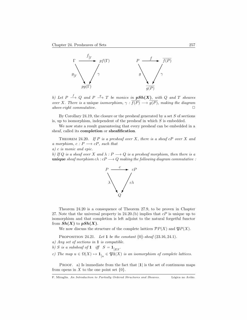
Chapter 24. Presheaves of Sets 257
Γ - pf(Γ)
g|Γ γ
pg(Γ)
f|Γ
AAAAAU
P - f(P )
g γ
g(P )
f
AAAAAU
b) Let Pf−→ Q and P
g−→ T be monics in pSh(X), with Q and T sheaves
over X. There is a unique isomorphism, γ : f(P ) −→ g(P ), making the diagramabove-right commutative. 2
By Corollary 24.19, the closure or the presheaf generated by a set S of sectionsis, up to isomorphism, independent of the presheaf in which S is embedded.
We now state a result guaranteeing that every presheaf can be embedded in asheaf, called its completion or sheafification.
Theorem 24.20. If P is a presheaf over X, there is a sheaf cP over X anda morphism, c : P −→ cP , such that
a) c is monic and epic.
b) If Q is a sheaf over X and λ : P −→ Q is a presheaf morphism, then there is aunique sheaf morphism cλ : cP −→ Q making the following diagram commutative :
P - cP
λ cλ
Q
c
AAAAAU
Theorem 24.20 is a consequence of Theorem 27.9, to be proven in Chapter27. Note that the universal property in 24.20.(b) implies that cP is unique up toisomorphism and that completion is left adjoint to the natural forgetful functorfrom Sh(X) to pSh(X).
We now discuss the structure of the complete lattices PP (X) and PP (X).
Proposition 24.21. Let 1 be the constant 0-sheaf (23.16, 24.1).
a) Any set of sections in 1 is compatible.
b) S is a subsheaf of 1 iff S = 1|ES.
c) The map u ∈ Ω(X) 7→ 1|u ∈ P1(X) is an isomorphism of complete lattices.
Proof. a) Is immediate from the fact that |1| is the set of continuous mapsfrom opens in X to the one point set 0.
F. Miraglia. An Introduction to Partially Ordered Structures and Sheaves. Logica no Aviao.
Chapter 24. Presheaves of Sets 258
b) For S ⊆ |1|, 23.12 implies that S ⊆ 1|ES . Since all sets of sections in 1 are
compatible, |S| is compatible and must glue to the unique map from ES to 0.But then S = 1|ES . The converse is clear, since all restrictions of a sheaf to an
open set are sheaves.
c) By (b), the map in (c) is bijective. To show that it is an isomorphism of completelattices, it is enough to prove that it is an isomorphism of posets, that is, for allu, v ∈ Ω(X),
u ≤ v iff 1|u ⊆ 1|v.One direction is obvious; the other follows from E1|u = u and the fact that support
is increasing, i.e., S ⊆ T ⇒ ES ≤ ET , completing the proof.
Proposition 24.21 shows that, in general, PP (X) will not be a Boolean algebra,since Ω(X) cannot be a Boolean algebra except in (very) special circumstances.Generalizing 24.21, we have
Theorem 24.22. PP (X) and PP (X) are frames, with ⊥ = ∅ (the empty sheaf)and > = P .
Proof. We treat the case of PP (X), leaving the other as an exercise. LetT , Sα, α ∈ A, be closed subsheaves of P . By 8.7, it is enough to prove that
T ∩∨Sα ⊆
∨α∈A (T ∩ Sα).
Since the restriction is that induced by P , this relation is equivalent to the inclusionof the respective domains. Let z ∈ |T ∩
∨Sα|; then, (∗) in 24.18 yields
Ez =⋃[[z = s]] : s ∈ |T | ∩ |
∨Sα|
=⋃[[z = s]] : s ∈ |T | ∩
⋃α∈A |Sα|
=⋃[[z = s]] : s ∈
⋃α∈A |T | ∩ |Sα|
and so z ∈ |∨α∈AT ∩Sα|, as desired.
Explicit formulas for implication and negation are the content of
Proposition 24.23. For S, T ∈ PP (X), P a presheaf over X, we have 8
a) |S → T | = x ∈ |P | : ∀ u ∈ Ω(X) (x|u ∈ |S| ⇒ x|u ∈ |T |).9
b) |¬S| = x ∈ |P | : ∀ u ∈ Ω(X), x|u 6∈ |S|.
Proof. a) The first step is verifying that the right-hand side of the equality,A, is a closed subpresheaf of P . If z ∈ |P | is such that
Ez =⋃a∈A [[a = z]],
and u ∈ Ω(X), assume that z|u ∈ |S|. For each a ∈ A, 23.7.(e) and [rest 3] in
23.7.(a) yield
a|u∩[[a=z]]= z|u∩[[a=z]]
,
8Exactly the same formulas hold for S, T ∈ PP (X).9The ⇒ here is classical material implication !
F. Miraglia. An Introduction to Partially Ordered Structures and Sheaves. Logica no Aviao.
Chapter 24. Presheaves of Sets 259
and so, S being a presheaf, it follows that a|u∩[[a=z]]∈ |S|. Since a ∈ A, we conclude
that a|u∩[[a=z]]∈ |T |. But then,⋃
a∈A [[x|u = a|u∩[[a=z]]]] =
⋃a∈A u ∩ [[a = z]] ∩ [[a = z]]
= u ∩⋃a∈A [[a = z]] = u ∩ Ez = Ez|u,
and z|u ∈ |T | because T is closed. Hence, A is a closed subpresheaf of P . We now
verify that for all Z ∈ PP (X)
S ∩ Z ⊆ T iff Z ⊆ A,
and so A = (S → T ). Assume that S ∩ Z ⊆ T , x ∈ |Z| and that z|u ∈ |S|, for
u ∈ Ω(X); then, since Z is a presheaf, z|u ∈ |S| ∩ |Z| = |S ∩ Z|. Hence, x|u ∈ |T |and x ∈ |A|. The converse is clear. Item (b) follows from (a) and the fact that¬S = (S → 0).
24.24. Image and Restriction of Morphisms Let Pη−→ Q be a morphism
of presheaves. If T is a subpresheaf of P , the restriction of η to T , η|T : T −→ Q, is
given by t ∈ |T | 7→ ηt ∈ |Q|. If one prefers to view it as a natural transformation,then
η|T = ηu|T (u): u ∈ Ω(X).
The image of η is defined as
Imη = ηx : x ∈ |P |,that is, the closure of the set-theoretical image of η. The set-theoretical image isa subpresheaf of Q, but it will not be a subsheaf, even if P and Q are sheaves.Hence, we prefer to use closure to uniformly obtain subobjects in pSh(X) andSh(X). In general, if S ⊆ |P |,
η∗S = ηs : s ∈ S,is the image of S by η. 2
Lemma 24.25. If η : P −→ Q is a morphism of presheaves, the mapη∗ : PP (X) −→ PQ(X) 10 is a
∨-morphism.
Proof. Let Si : i ∈ I ⊆ PP (X); it is clear that η∗ is increasing, and so itis enough to check that
η∗(∨i∈I Si) ⊆
∨i∈I η∗Si.
Since⋃|Si| is dense in
∨Si (Corollary 24.18), 24.16.(c) yields, for y ∈ |η∗(
∨i∈I Si)|,
Ey =⋃s∈
∨Si
[[y = ηs]] =⋃s∈
⋃|Si| [[y = ηs]]
=⋃i∈I
⋃s∈|Si| [[y = ηs]] =
⋃i∈I
⋃z∈|η∗Si| [[y = z]] 11
=⋃t∈
⋃|η∗Si| [[y = t]],
and so y ∈ |∨i∈Iη∗Si|, as needed.
10Defined in 24.24.11Because ηs : s ∈ |Si| is dense in η∗Si and 24.16.(c).
F. Miraglia. An Introduction to Partially Ordered Structures and Sheaves. Logica no Aviao.

Chapter 24. Presheaves of Sets 260
24.26. Inverse Image. Let Pη−→ Q be a morphism of presheaves. If S is a
subpresheaf of Q, the map
u ∈ Ω(X) 7→ η−1u (S(u)) ⊆ P (u),
with the restrictions induced by P , is a subpresheaf of P , the inverse image of Sby η and written η−1(S). Notice that the domain of the inverse image is given by
|η−1(S)| = s ∈ |P | : ηs ∈ |S|,that is, the set-theoretic inverse image. It is well-known that in the case of sets, in-verse image is well-behaved, preserving all set-theoretic operations. The analogousproperties in our present setting are described in Proposition 24.27. 2
Proposition 24.27. Let η : P −→ Q be a morphism of presheaves.
a) For S, T ⊆ |Q|, S dense in T ⇒ η−1S is dense in η−1T . Moreover,
(1) η−1(T ) = η−1T ; (2) T ∈ PQ(X) ⇒ η−1T ∈ PP (X).
b) The map η∗ : PQ(X) −→ PP (X), S 7→ η−1(S), is an open frame-morphism.
c) The pair 〈 η∗, η∗ 〉 satisfies, for S ∈ PP (X) and T ∈ PQ(X),
[adj] η∗S ⊆ T iff S ⊆ η∗T ,
being therefore an adjoint pair (4.6, 7.8), with η∗ left adjoint to η∗.
d) η∗ is monic iff η is epic.
Proof. a) Let S ⊆ Q and x ∈ η−1T ; then ηx ∈ T and so
Eηx =⋃s∈S [[ηx = s]]. (I)
Let A = x|[[ηx=s]]: s ∈ S; then, for all s ∈ S, condition (ii) in 23.19.(2) and
23.7.(e) yield η(x|[[ηx=s]]) = (ηx)|[[ηx=s]]
= s|[[ηx=s]]∈ |S|, and so y|[[ηx=s]]
∈ η−1S,
i.e., A ⊆ η−1S. Hence, since Eηx = Ex, (I) entails⋃s∈S [[x = y|[[ηx=s]]
]] =⋃s∈S [[ηx = s]] ∩ [[x = x]] =
⋃s∈S [[x = s]]
= Eηx = Ex,
showing that x ∈ A ⊆ η−1S, as desired. To get the full conclusion in (a), recallthat a subset of |P | is dense in the presheaf it generates and that denseness istransitive (24.15.(a), 24.16.(b)). For (1), since T is dense in T and T ⊆ T , we have
η−1T dense in η−1(T ) and η−1T ⊆ η−1(T ),
and we conclude by 24.16.(d). Item (2) follows immediately from (1).
b) Let Ti : i ∈ I ⊆ PQ(X). Since (set-theoretical) inverse image preservesarbitrary intersections, it is clear that η∗ is a
∧-morphism. For joins, we have,
using (a).(1)
η∗(∨Ti) = η∗(
⋃i∈I |Ti|) = η∗(
⋃i∈I |Ti|)
=⋃i∈I η
∗Ti =∨η∗Ti.
Since η∗ preserves meets, if S, T ∈ PQ(X), then
η∗S ∩ η∗(S → T ) = η∗(S ∩ (S → T )) ⊆ η∗T ,
and so η∗(S → T ) ⊆ (η∗S → η∗T ) 12. To prove the reverse inclusion, it is enoughto show, by the adjointness condition [→] in 6.1, that for A ∈ PP (X),
12Note : this argument is valid for any ∧-semilattice morphism between HAs.
F. Miraglia. An Introduction to Partially Ordered Structures and Sheaves. Logica no Aviao.

Chapter 24. Presheaves of Sets 261
A ∩ η∗S ⊆ η∗T ⇒ A ⊆ η∗(S → T ). (*)
For x ∈ |A|, assume that (ηx)|u ∈ |S|, u ∈ Ω(X). From ηx|u = η(x|u), it follows
that x|u ∈ |A| ∩ |S| = |A ∩ S|. The hypothesis in (*) entails x|u ∈ η∗T , that is,
η(x|u) ∈ T . This reasoning (and 24.23.(a)) proves that ηx ∈ |S → T |, completing
the proof of (b).
Item (c) is straightforward and left to the reader. For (d), observe that 7.9.(a)guarantees that η∗ is monic (i.e., injective) iff η∗ is onto. Hence, it is enough toshow that η∗ is onto iff η is an epic. If η∗ is onto PQ(X), then
η∗P = Q = ηx : x ∈ |P |,showing that the set-theoretical image of |P | by η is dense in Q. By 24.6.(b), η is anepic. If η is epic and S ∈ PQ(X), it is left to the reader to show that η∗η
∗S = S,completing the proof.
Since we have products and the notion of subobject in pSh(X), we can gen-eralize Definition 18.15, as follows :
Definition 24.28. Let Ai, i ∈ I, be a family of presheaves over X and
let A =∏i∈I Ai. Let P be a presheaf and A
f−→ P be a morphism. Let S be asubpresheaf of A and let J be a subset of I.
a) f depends only on J iff for all u ∈ Ω(X), fu : A(u) −→ P (u) depends onlyon J , that is, if s = 〈 si 〉 and t = 〈 ti 〉 are sections in A(u), then
J ⊆ i ∈ I : si = ti implies fu(s) = fu(t).
b) S depends only on J iff for all u ∈ Ω(X) and all s = 〈 si 〉, t = 〈 ti 〉 in A(u),
J ⊆ i ∈ I : si = ti and s ∈ S(u) implies t ∈ S(u).
24.29. Notation. Let n ∈ N and let A be a non-empty set. For s = 〈 si 〉 ∈ An,for k ∈ (n+ 1) and a ∈ A, define 〈 a/k; s 〉 ∈ An+1, by
〈 a/k; s 〉(i) =
si if i < k
a if i = k
s(i−1) if i > k.
Hence, 〈 a/k; s 〉, corresponds to constructing the (n+ 1)-tuple that has si in thefirst (k−1) coordinates, has a in the kth coordinate, and has si−1 in the coordinatesindexed by i > k. This notation applies both to sections over an open set in powersof a presheaf, as well as to sections in powers of the domain of a presheaf. 2
24.30. Quantifiers. Let P be sheaf over X and let S be a subsheaf of Pn,n ∈ N. For k ∈ n, let πk : Pn −→ P (n−1), be the projection that forgets the kth
coordinate. What are the meanings of ∃xk S and ∀xk S ? The classical answers inSet are
(I)
∃xk S = Im πk;
∀xk S = largest A ⊆ P (n−1), such that π−1k (A) ⊆ S
= s ∈ P (n−1) : For all t ∈ P , 〈 t/k; s 〉 ∈ S.
F. Miraglia. An Introduction to Partially Ordered Structures and Sheaves. Logica no Aviao.

Chapter 24. Presheaves of Sets 262
Because these answers are “structural”, it is natural to use the same ideas todefine these concepts in Sh(X). Thus, in view of 24.24, define,
[∃xk S](u) = z ∈ P (u)(n−1) :
∃ ui ≤ u and ti ∈ P (ui), i ∈ I,
such that⋃ui = u and
〈 ti/k; z|ui 〉 ∈ S(ui), i ∈ I.
[∃]
Then, u 7−→ [∃xk S](u), with restrictions induced by P (n−1), is a subpresheaf ofP (n−1), the existential quantification along the kth component.
For the universal quantifier, one might be tempted to consider
A(u) = z ∈ [P (u)](n−1) : For all t ∈ P (u), 〈 t/k; z 〉 ∈ S(u).But observe that, for v ⊆ u, if the restriction map of P is not onto, then u 7→ A(u)will not be a presheaf. Thus, we are led to define
[∀xk S](u) = z ∈ P (u)(n−1) :For all v ∈ Ω(u) and t ∈ P (v),
〈 t/k; z|v 〉 ∈ S(v)
[∀]
which, with restrictions induced by P (n−1), is a subpresheaf, the universal quan-tification of S along the kth component. The reader can then verify that we have
Fact 24.31. If S ⊆ Pn depends only on α, then (∃xk S) and (∀xk S) dependonly on α − k. 2
By 24.75, S can be considered as a subpresheaf of Pα, namely πα(S), whereπα : Pn −→ Pα is the map that forgets the coordinates outside α. Moreover,
πα−1(πα(S)) = S. (II)
Fact 24.31 and (II) imply that if k 6∈ α, then
(∃xk S) = (∀xk S) = S. (III)
Moreover, if S ⊆ Pn, after quantifying, existentially or universally, with respectto all components on which S depends, we obtain a subsheaf of the final object 1,that is, an open set in X (24.21). 2
3. Relations and Quotients
In this section we develop an elementary theory of relations in pSh(X). Afull blown theory will emerge when we discuss characteristic maps in Part 7.
As is well known in the case of sets, a relation from A to B is a subset of A × B.This can, of course, be generalized to any set of components. In particular, if n isa positive integer, a n-ary relation on a set A is a subset of An. In pSh(X), theconcept is analogous, with one subtlety :
Definition 24.32. If P , Q are presheaves over X, a relation from P toQ is a closed subpresheaf of P × Q. If n ≥ 1 is an integer, a n-ary relationon P is a closed subpresheaf of Pn.
Thus, a relation from P to Q consists of
∗ For each u ∈ Ω(X), a subset R(u) ⊆ P (u) × Q(u);
∗ For v ≤ u, 〈 s, t 〉 ∈ R(u) ⇒ 〈 s|v, t|v 〉 ∈ R(v);
F. Miraglia. An Introduction to Partially Ordered Structures and Sheaves. Logica no Aviao.

Chapter 24. Presheaves of Sets 263
∗ If 〈x, y 〉 ∈ |P × Q| is such that
Ex = Ey =⋃〈s,t〉∈|P×Q| [[x = s]] ∩ [[y = t]],
then 〈x, y 〉 ∈ |R| 13. Write ∆ for ∆2, the diagonal of P 2.
If R is a relation from P to Q, its inverse, R−1 is defined by
R−1(u) = 〈 t, s 〉 ∈ Q(u) × P (u) : 〈 s, t 〉 ∈ R(u),with restriction induced by Q × P ; clearly, R−1 is a closed subpresheaf of Q × P .
Binary relations can be composed. Care must be exercised in transcribing theusual set-theoretic definition, so as to furnish closed subpresheaves. This idea isused so often that we take time to explain it.
Let R be relation from P to Q and S a relation from Q to T . By analogy withthe set-theoretic case, consider, for each u ∈ Ω(X)
C(u) = 〈 s, t 〉 ∈ P (u) × T (u) :∃ z ∈ Q(u), such that
〈 s, z 〉 ∈ R(u) and 〈 z, t 〉 ∈ S(u)
with restrictions induced by P × T ; C is a subpresheaf of P × T , but will not,in general, be closed. We are then led to define the composition of R and S asthe closure of C in P × T . Hence, for u ∈ Ω(X) and 〈 s, t 〉 ∈ P (u) × T (u)
〈 s, t 〉 ∈ (S R)(u)
iff
∃ ui ≤ u and zi ∈ Q(ui) such that u =⋃ui and ∀ i ∈ I,
〈 s|ui , zi 〉 ∈ R(ui) and 〈 zi, t|ui 〉 ∈ S(ui).
Hence, the distinction between C and (S R) is that one must use the set-theoretical idea locally. One way to further understand this is to realize that(S R) is the image by a morphism of the relation
〈 s, z, t 〉 ∈ |P ×Q× T | : 〈 s, z 〉 ∈ |R| and 〈 z, t 〉 ∈ |S|.Next, we discuss equivalence relations in pSh(X).
Definition 24.33. If P is a presheaf over X, an equivalence relation onP is a binary relation E on P such that :
[ER1] : ∆ ⊆ E; [ER2] : E = E−1; [ER3] : E E ⊆ E.
The following observations are straightforward :
I. For each u ∈ Ω(X), E(u) is a (set-theoretic) equivalence relation on P (u);
II. The intersection of a family of equivalence relations on P is an equivalencerelation on P ;
III. P × P is the largest and ∆ is the smallest equivalence relation on P ; the setof equivalence relations on a presheaf is a complete lattice under inclusion.
Item (III) allows us to set down
Definition 24.34. If P is a presheaf over X and R ⊆ P × P , the equiva-lence relation generated by R is
E(R) =⋂E ⊆ P × P : E is an equivalence relation and R ⊆ E.
13Notation as in 24.2.
F. Miraglia. An Introduction to Partially Ordered Structures and Sheaves. Logica no Aviao.

Chapter 24. Presheaves of Sets 264
Example 24.35. Let Pλ−→ Q be a morphism. The set
|ker(λ)| = 〈 s, t 〉 ∈ |P × P | : λs = λtis the domain of an equivalence relation on P , called the kernel of λ. Note thatker(λ) is the inverse image of the diagonal of Q × Q by the canonical morphism
λ × λ : P × P −→ Q × Q,
and so a closed subpresheaf of P × P , by 24.27.(a). Clearly, ker(λ) is the equalizer(24.4) of the pair 〈λ, λ 〉. Moreover, if R ⊆ P × P is a binary relation on P , then
(*) ∀ 〈 s, t 〉 ∈ |R|, λs = λt iff E(R) ⊆ ker(λ). 2
Let E be an equivalence relation on P and let v ≤ u be opens in X. Since E isa subpresheaf of P × P , for all s, t ∈ P (u), if s and t are equivalent with respectto E(u), then s|v and t|v are equivalent with respect to E(v). Thus, if
[P/E](u) = P (u)/E(u) = s/E(u) : s ∈ P (u),is the set of equivalence classes of P (u) with respect to the E(u), the map
[P/E](u) −→ [P/E](v), s/E(u) 7→ s|v/E(v)
is a well defined restriction on P/E, making it a presheaf over X, the quotientof P by the equivalence E. The natural map, πE : P −→ P/E, defined by
s ∈ P (u) 7−→ s/E(u) ∈ P (u)/E(u)
is a morphism of presheaves, the projection or quotient morphism. SinceE = ker(πE), every equivalence relation is the kernel of a morphism (24.35).
As an application, we can construct, in pSh(X), the coequalizer of a pair ofmorphisms, λ, µ : P −→ Q. Let E be the equivalence relation on Q, generated bythe subpresheaf R of Q × Q, whose domain is given by
|R| = 〈λs, µs 〉 : s ∈ |P |.By (*) in 24.35, πE λ = πE µ, where πE : Q −→ Q/E is the quotient morphism.〈Q; πE 〉 is the coequalizer of the pair (λ, µ), that is, it has the following universalproperty (16.30) :
If Qf−→ T is a presheaf morphism and f λ = f µ, then there is a unique
g : Q/E −→ T , such that f = g πE :
Q - Q/E
πE g
T
f
AAAAAU
Write Coeq(λ, µ) for the coequalizer of the pair (λ, µ).
In general, it is not true that if P/E is a sheaf when P and E are sheaves.However, Theorem 24.20 applies to yield a completion of P/E, which is defined asthe quotient of the sheaf P by the equivalence relation E in the category Sh(X).
F. Miraglia. An Introduction to Partially Ordered Structures and Sheaves. Logica no Aviao.
Chapter 24. Presheaves of Sets 265
Similarly, the coequalizer of a pair of morphisms in Sh(X) is the completion ofthe construction presented above for presheaves.
Theorem 16.31, together with the constructions in this section and in section24.1, yield
Theorem 24.36. Sh(X) and pSh(X) are complete and cocomplete cate-gories.
4. The Sheaf of Subsheaves. Exponentiation
In the category Set, an important object is the family of subsets of a set andthe family of maps between two sets. These concepts are of course related, becausethe set 0, 1 = 2 has a special role : there is a natural and bijective correspondencebetween subsets of A and functions from A to 2.
In this section, we discuss what sheaf plays the role of 2 in Sh(X), as well asexponentiation. We shall focus, mainly, on the category Sh(X), because it is themost important case. To treat these themes for presheaves or closed presheaves allthat is needed are minor modifications and/or the use of Theorem 24.20.
To construct an analogue of the power set in Sh(X), we must find a sheafthat fulfills that role. The next definition sets down the concept we need.
Definition 24.37. Let Q be a sheaf over the topological space X. With no-tation as in 23.12, for u ∈ Ω(X), set
PQ(u) = T ⊆ Q : T is a subsheaf of Q|u.For v ≤ u in X, there is a natural restriction map
|v : PQ(u) −→ PQ(v), given by T 7−→ T|v.
The association u ∈ Ω(X) 7−→ PQ(u), together with the restriction maps |v defined
above, constitute a presheaf written PQ.
Note that the set of global sections of PQ is precisely PQ(X), which is aframe by Theorem 24.22, but in general, not a cBa. This points to a fundamentaldifference between the categories Set and Sh(X) : the analogue of the power setis a frame, not a cBa.
Recall (23.6.(c)) that the support of a sheaf Q is the open set
EQ =⋃u ∈ Ω(X) : Q(u) 6= ∅.
Clearly, EQ|u ⊆ u. Hence, an alternate description of PQ is :
i) |PQ| = 〈S, u 〉 ∈ PQ(X) × Ω(X) : ES ⊆ u;ii) For 〈S, u 〉 ∈ |PQ| and v ∈ Ω(X), set 〈S, u 〉|v = 〈S|u∩v, v 〉;
iii) For 〈S, u 〉, 〈T, v 〉 ∈ |PQ|,[[〈S, u 〉 = 〈T, v 〉]] =
⋃w ∈ Ω(u ∩ v) : S|w = T|w
=⋃w ∈ Ω(u ∩ v) : S(w) = T (w).
Perhaps a comment is in order regarding the equalities in (iii). To say that twosheaves are the same or equal is to say that the corresponding functors are
F. Miraglia. An Introduction to Partially Ordered Structures and Sheaves. Logica no Aviao.

Chapter 24. Presheaves of Sets 266
the same. However, if S and T are subsheaves of a sheaf Q, since restrictions arethose induced by Q, S will be equal to T if and only if they have the same set ofsections over all opens in X. This leads from the second to the third term in (iii).The last description can be seen to be equivalent to the (classical) one in 24.37,by realizing that PQ(u) can be identified with the set of pairs 〈S, u 〉, where S isa subsheaf of Q with support contained in u.
Note that for all S ∈ PQ(u), ES = [[S = S]] = u.
Proposition 24.38. Let Q be sheaf over X.
a) For u ∈ Ω(X), PQ(u) is a frame, with Q|u as its top and ∅ as its bottom.
Implication and pseudo-complementation in PQ(u) are given by the following pre-scriptions, where w ∈ Ω(u) and the restrictions are those induced by Q :
(S → T )(w) = s ∈ Q(w) : ∀ v ≤ w, s|v ∈ S(v) ⇒ s|v ∈ T (v);
¬ S(w) = s ∈ Q(w) : ∀ v ≤ w, v 6= ∅ ⇒ s|v 6∈ S(v).b) The restriction maps, |v : PQ(u) −→ PQ(v), S 7−→ S|v, are open frame
morphisms.
c) PQ is a sheaf over X.
Proof. Left to the reader; the main ingredients, besides the comments justmade on equality and restriction in PQ, are the computations used in the proofof 24.22 and 24.23.
The sheaf PQ is the sheaf of subsheaves of Q.
If Q ∈ Sh(X), the sheaf PQ has a special property, called flabbyness, whosedefinition is item (a) of
Proposition 24.39. Let Q and P be sheaves over X.
a) For all u ∈ Ω(X), the restriction map from PQ(X) to PQ(u) is surjective 14.In particular, PP (X) is dense in PQ.
b) Let λ, µ be morphisms from PQ to P . Then, λ = µ iff λX = µX .
c) There is a natural bijective correspondence between the set of morphisms fromPQ to P and the set of maps from PQ(X) to P (X), given by λ 7→ λX .
Proof. a) Since Q|u is a subsheaf of Q, all of its subsheaves are subsheaves
of Q. The density assertion is now obvious. Item (b) is an immediate consequenceof the fact that global sections are dense and 24.14.
c) Let PQλ−→ P be a sheaf morphism. If 〈S, u 〉 is a section in PQ, then
λu(〈S, u 〉) = λX(〈S,X 〉)|u,
and so the values of λ are entirely determined by those of λX . The remainingstatements follow from this and item (b).
14Or equivalently, every section in PQ can extended to a global section (i.e., an element ofPQ(X)); see also 31.10.(e)
F. Miraglia. An Introduction to Partially Ordered Structures and Sheaves. Logica no Aviao.

Chapter 24. Presheaves of Sets 267
Our next result shows that the sheaf Ω of opens in X (23.13) is a subobjectclassifier. Before the statement, we need the following
24.40. Notation. Let Q be a sheaf over X.
a) For S ∈ PQ(X) and u ∈ Ω(X), define
γSu : Q(u) −→ Ω(u), by γSu(s) = v ≤ u : ∃ t ∈ Q(v), with s|v = t.
The family γS = γSu : u ∈ Ω(X) is a morphism from Q to Ω, the characteristicmorphism of S.
b) Let λ : Q −→ Ω be a morphism. For u ∈ Ω(X), define
Qλ(u) = s ∈ Q(u) : λus = u.With restrictions induced by Q, Qλ is a subsheaf of Q, the characteristic sub-sheaf of λ. 2
With these preliminaries, the reader is invited to prove
Theorem 24.41. Let Q be a sheaf over X. With notation as above, the mapsS ∈ PQ(X) 7→ γS : Q −→ Ω
λ : Q −→ Ω 7→ Qλ ∈ PQ(X),
are inverse bijective correspondences between PQ(X) and the set of all sheaf mor-
phisms from Q to Ω. 2
One of the fundamental laws in Set is the existence of a natural bijective
correspondence between AB×C and ABC
, i.e., between [B × C, A] and [C, AB ],where [X, Y ] is the set of morphisms from X to Y , as in Chapter 16. An importantingredient in this adjunction is the concept of “evaluation at a point” :
ev : AB × B −→ A, given by 〈 f, b 〉 7→ f(b).
Indeed, the correspondence mentioned above can be constructed as follows : for a
morphism Cλ−→ AB , consider
λ × IdB : C × B −→ AB × B, defined by 〈 c, b 〉 7→ 〈λ(c), b 〉;we associate to λ the map g = ev (λ × IdB) from C × B to A :
C × B - AB × B
g ev
A
λ× IdB
AAAAAU
Note that the construction is entirely categorical. This same law holds in Sh(X),once the appropriate concepts have been defined.
Recall that if λ : P −→ Q is a morphism of sheaves and S is a subsheaf of P ,the restriction of λ to S is the morphism
λ|S : S −→ Q, given by s 7→ λs.
F. Miraglia. An Introduction to Partially Ordered Structures and Sheaves. Logica no Aviao.
Chapter 24. Presheaves of Sets 268
If u ∈ Ω(X), define λ|u as the restriction of λ to the subsheaf P|u. Observe that,
in fact, λ|u : P|u −→ Q|u. Further, if v ≤ u in X, then (λ|u)|v = λ|v. In particular,
if QP (u) is the set of morphisms from P|u to Q|u and v ≤ u in X, there is a map
|v : QP (u) −→ QP (v), given by λ 7→ λ|v.
These assignments constitute a contravariant functor, QP , from Ω(X) to Set, i.e.,a presheaf over X. For λ ∈ QP (u) and µ ∈ QP (v), we have
[[λ = µ]] =⋃w ∈ Ω(u ∩ v) : λ|w = µ|w
=⋃w ∈ Ω(u ∩ v) : ∀ s ∈ P (w), λs = µs.
It is now straightforward that QP is a sheaf over X.
Definition 24.42. Let P and Q be sheaves over X. With notation as above,the sheaf QP is defined to be the sheaf of morphisms from P to Q.
Define the evaluation morphism ev : QP × P −→ Q, as the natural trans-formation ev = evu : u ∈ Ω(X), where
evu : QP (u) −→ Q(u) is given by evu(λ, s) = λs.
Proposition 24.38 now yields
Corollary 24.43. The correspondences in Theorem 24.41 extend to iso-
morphisms between the sheaves PQ and ΩQ
. 2
With the same proof as in Set, we have
Theorem 24.44. In Sh(X), exponentiation and Cartesian product are ad-joints that is, if P , Q and R are sheaves, there is a natural sheaf isomorphism
between QP×R and QPR
, given by
λ ∈ [R, QP ] 7→ ev (λ × IdR) ∈ [P × R, Q],
where ev is the evaluation morphism of 24.42. 2
Remark 24.45. Since Sh(X) has finite products and the adjunction in 24.44,it is, like Set, a Cartesian closed category (see [44], section IV.6, p.95 ff). 2
In Part 7 we shall return to the theme of 24.41, describing a theory of char-acteristic functions, fundamental in treating first-order structures in pSh(X).
5. Constant Sheaves
Let A be a set and A be the constant A sheaf over X, as in 23.16 and 23.17.By definition, for each u ∈ Ω(X), A(u) consists of the set of continuous maps,s : u −→ A, where A has the discrete topology (all points as open).
We can identify A with the set of constant maps from X to A : for a ∈ A,
write a for the constant map of value a on X. Write A for the image of A in A(X)by the injection a 7−→ a.
For s ∈ |A| and a ∈ A, s−1(a) = [[s = a]], which is clopen in Es. Thus,
[[s = a]] 6= ∅ iff a ∈ Ims.
F. Miraglia. An Introduction to Partially Ordered Structures and Sheaves. Logica no Aviao.

Chapter 24. Presheaves of Sets 269
Furthermore, if a 6= b in A, then [[s = a]] ∩ [[s = b]] = ∅. We summarize some ofthe basic properties of sections of constant sheaves in
Lemma 24.46. Let A be a set, f ∈ AX , s, t ∈ |A| and u ∈ Ω(X).
a) f ∈ |A| iff for all a ∈ A, [[f = a]] is clopen in X.
b) Es =⋃a∈Ims [[s = a]], this union being composed of pairwise disjoint non-
empty clopens in Es. Moreover,
(1) For all a ∈ Ims, s|[[s=a]]= a|[[s=a]]
; (2) A is dense in A.
c) [[s = t]] = x ∈ Es ∩ Et : s(x) = t(x).d) [[s = t]] is clopen in Es ∩ Et.e) If f = 〈 f1, . . . , fn 〉 ∈ A(u)n, then there are non-empty pairwise disjoint clopensin u, ui : i ∈ I, such that u =
⋃i∈I ui and each fk is constant on ui, for all
i ∈ I and 1 ≤ k ≤ n.
f) Let 〈 ti, ui 〉 ∈ A(X) × Ω(u), i ∈ I, be such that
(1) ui : i ∈ I are pairwise disjoint non-empty clopens in u;
(2) u =⋃i∈I ui;
Then, there is s ∈ A(u), such that for all i ∈ I, s|ui = ti|ui .
g) If u is clopen in X, then the restriction map from A(X) to A(u) is a surjection.
Proof. (a) is just a restatement of the fact that f is continuous. Item (b) isclear; to verify (c), recall that
[[s = t]] =⋃w ∈ Ω(Es ∩ Et) : s|w = t|w
⊆ x ∈ Es ∩ Et : s(x) = t(x).Now, if s(x) = t(x) = a, then x ∈ [[s = a]] ∩ [[t = a]] = w, a clopen subset ofEs ∩ Et, such that s|w = t|w. But this implies the equality in (c).
d) To show that [[s = t]] is clopen in Es ∩ Et, let x ∈ Es ∩ Et satisfy s(x) = a6= t(x). Then, x ∈ [[s = a]] ∩ Et, a clopen in Et, and
[[s = a]] ⊆ x ∈ Es ∩ Et : s(y) 6= t(y).Thus, the complement of [[s = t]] is open in Es ∩ Et, as needed. Item (e) followsfrom (b) and 8.4.
f) Just observe that the family ti|ui : i ∈ I is compatible and so can be glued
to a section s over u.
g) Fix s ∈ A(u) and a ∈ A; since the sections a|(X−u)and s have disjoint extents
whose union is X, (d) implies that there is t ∈ A(X) such that t|Es = s, as
desired.
Remark 24.47. It is well known (and easy to verify) that if Yi are topologicalspaces, i ∈ n, then 15
C(X,∏Yi) is naturally isomorphic to
∏C(X,Yi),
15n = 1, . . . , n, as in page 15.
F. Miraglia. An Introduction to Partially Ordered Structures and Sheaves. Logica no Aviao.

Chapter 24. Presheaves of Sets 270
where∏Yi has the product topology. Since the finite product of discrete spaces
is discrete, the finite product of constant Ai sheaves is naturally isomorphic to theconstant
∏Ai sheaf. 2
Remark 24.48. A map Af−→ B induces a morphism (23.18)
Af−→ B, given by s 7−→ f s.
This produces a covariant functor from Set to the category of constant sheavesover X, that preserves monics and epics. 2
The next result characterizes morphisms whose domain is a constant sheaf.
Proposition 24.49. Let Q be a presheaf over X, let A be a set and letλ, µ: A −→ Q be presheaf morphisms.
a) The following are equivalent : 16
(1) λ = µ. (2) λX |A = µX |A.
b) If Q is a sheaf, then the map τ : [A, Q] −→ Q(X)A, λ 7→ λX |A, is a
natural bijective correspondence between the morphisms from A to Q and the setof maps from A to the set of global sections of Q, Q(X).
Proof. a) Since A is dense in A, (1) ⇔ (2) follows from 24.14.
b) It is enough to verify that every f ∈ Q(X)A gives rise to a morphism, whose
restriction to A is f (24.14). For s ∈ |A|, consider the family
T = fa|[[s=a]]: a ∈ A ⊆ |Q|.
Since A is a dense set of global sections in A,
Es =⋃a∈A [[s = a]] =
⋃a∈A fa|[[s=a]]
.
Hence, T is compatible, and there is a unique t ∈ |Q|, such that for all a ∈ A,
Et = Es and t|[[s=a]]= fa|[[s=a]]
.
Define λs = t. It is straightforward that λ is a morphism, such that λX |A = f .
In particular, we have
Corollary 24.50. Let P be a presheaf over X. There is a natural bijectivecorrespondence between the morphisms from 1 to P and the set of global sectionsof P , P (X), given by
λ ∈ [1, P ] 7→ λX(0) ∈ A(X).
where 0 is the constant map with value 0 17.
We now return to the consideration of constant sheaves of L-structures as in23.17. Let X be a topological space, let L be a first-order language with equalityand M a L-structure. We know from 23.17 that M and Mb are presheaves ofL-structures, with relations, constants and operations defined pointwise. We know
16Recall that λ = λu : u ∈ Ω(X).170 is the unique element of 1(X).
F. Miraglia. An Introduction to Partially Ordered Structures and Sheaves. Logica no Aviao.

Chapter 24. Presheaves of Sets 271
that M is a sheaf over X. To characterize the type of completeness of Mb weintroduce
Definition 24.51. Let C be a category. A C-presheaf P over X is finitelycomplete if all finite compatible sets of sections in P have a unique gluing. Thatis, if S ⊆f |P | is compatible, then there is a unique t ∈ |P | such that
Et =⋃s∈S Es and t|Es = s, for all s ∈ S.
Proposition 24.52. Mb is a finitely complete presheaf over X.
Proof. If S ⊆f |Mb| is compatible, since continuity is a local property, 1.2yields a continuous t :
⋃s∈S −→ M , whose restriction to each Es is s ∈ S. Since
S is finite and all sections in S have finite image, the same must be true of t.
Definition 24.53. Let φ(v1, . . . , vn) be a formula in L, in the free variablesv1, . . . , vn. Let u ∈ Ω(X) and f = 〈 f1, . . . , fn 〉 ∈ M(u)n. Define
vu(φ)(f) = x ∈ u : M |= φ[f1(x), . . . , fn(x)]called the Feferman-Vaught value of φ at f 18. When u is clear from context,its mention will be omitted.
Recall (17.4) that a formula is primitive if it is of the form ∃xφ, where φ is aconjunction of atomic formulas. Note that the set of primitive formulas is closedunder conjunction.
Proposition 24.54. Let u ∈ Ω(X) and f ∈ M(u)n. Notation as above,
a) If φ(v1, . . . , vn) is a formula in L, then vu(φ)(f) is clopen in u.
b) Let ∆ be the set of formulas φ(v1, . . . , vn) in L such that
[∆] For all f ∈ M(u)n, M(u) |= φ[f ] iff vu(φ)(f) = u.
Then, ∆ is closed under conjunction and contains all primitive formulas in L.
c) Let Γ be the set of formulas φ(v1, . . . , vn) in L such that
[Γ] For all f ∈ M(u)n, vu(φ)(f) = u ⇒ M(u) |= φ[f ].
Then,
(1) φ, ψ ∈ ∆ ⇒ (φ → ψ) ∈ Γ; (2) φ ∈ Γ ⇒ ∀ z φ ∈ Γ.
d) Let σ be a sentence of the form ∀z (φ → ∃ y ψ), where φ, ψ are conjunctions ofatomic formulas. Then,
M |= σ ⇒ M(u) |= σ.
Proof. a) By 24.46.(e), there is a partition of u into clopens, ui : i ∈ I,such that all fk are constant in ui, i ∈ I. Write aik for the constant value of fk onui. Consequently
v(φ)(f) =⋃ui : M |= φ[ai1, . . . , a
in]
and
v(¬φ)(f) =⋃ui : M |= ¬φ[ai1, . . . , a
in].
18In honor of the seminal [14]; see Theorem 24.55.
F. Miraglia. An Introduction to Partially Ordered Structures and Sheaves. Logica no Aviao.
Chapter 24. Presheaves of Sets 272
Hence, u is the union of the disjoint opens v(φ)(f) and v(¬φ)(f), and both thesevalues are clopen in u.
b) Note that atomic formulas are in ∆ because M(u) is, by definition, a substruc-ture of Mu with the L-interpretation given in 17.9. It is straightforward that ∆ isclosed under conjunctions. Next, we show
(*) φ ∈ ∆ ⇒ ∃zφ ∈ ∆.
For 〈 g; f 〉 ∈M(u)n+1, suppose that M(u) |= φ[g; f ]. Then, for all x ∈ u,
M |= φ[g(x); f(x)]
and so v(∃zφ)(f) = u. If this equality holds, let ui, i ∈ I, be a clopen partitionof u, such that fk is constant in ui, 1 ≤ k ≤ n (24.46.(e)). Let ai1, . . . , a
in be the
values of f1, . . . , fn on ui. Since M |= ∃zφ[z; ai1, . . . , ain], there are bi ∈ M , such
that
For all i ∈ I, M |= φ[bi; ai1, . . . , a
in].
Let g : u −→M be the map that on each ui has constant value bi. Then, g ∈M(u)and v(φ)(g; f) = u. Since φ ∈ ∆, we get M(u) |= φ[g; f ], and so M(u) |= ∃zφ[f ],completing the proof of (*) and of item (b).
c) (1) Suppose φ, ψ ∈ ∆ and v(φ → ψ)(f) = u. If M(u) |= φ[f ], then v(φ)(f) =u and so v(ψ)(f) = u. But then, the hypothesis that ψ ∈ ∆ yields M(u) |= ψ[f ],as needed.
(2) Suppose that φ ∈ Γ and v(∀zφ)(f) = u. For g ∈M(u) and x ∈ u, we have
M |= φ[g(x); f(x)]
because M |= ∀zφ[z; f(x)]. Hence, v(φ)(g; f) = u, and the hypothesis that φ ∈ Γentails M(u) |= φ[g; f ]. Since g is arbitrary in M(u), we obtain M(u) |= ∀zφ[f ],as desired.
d) It is immediate from (b) and (c) that σ ∈ Γ. Since the hypothesis is equivalentto v(σ) = u, we conclude that M(u) |= σ, as claimed.
As a consequence of 24.54.(d), the L-structure of locally constant functions onany topological space with values in a model of a theory T whose axioms are of theform ∀z(φ → ∃yψ), with φ, ψ a conjunction of atomic formulas, are also modelsof T . This applies to many interesting mathematical structures, such as groups,rings, lattices, Boolean or Heyting algebras, etc.
The satisfaction of general formulas in the global sections of Mb is character-ized by the following fundamental result :
Theorem 24.55. (Feferman-Vaught) Let M be a L-structure and X a Booleanspace. To each formula φ(v1, . . . , vn) in L we can recursively associate a sequence
〈Φ(x1, . . . , xm); ψ1(v1, . . . , vn), . . . , ψm(v1, . . . , vn) 〉such that
∗ Φ(x1, . . . , xm) is a formula of the language of Boolean algebras;
∗ For 1 ≤ k ≤ m, ψk(v1, . . . , vn) are L-formulas in the same free variables as φ;
∗ For all f = 〈 f1, . . . , fn 〉 ∈ Mb(X)n,
Mb(X) |= φ[f1, . . . , fn] iff B(X) |= Φ[v(ψ1)(f), . . . , v(ψm)(f)].
F. Miraglia. An Introduction to Partially Ordered Structures and Sheaves. Logica no Aviao.

Chapter 24. Presheaves of Sets 273
Proof. By induction on the complexity of formulas. The proof given in [14]or [7] is easily adapted to this case, via 24.46, once it is remarked that the passagethrough the existential quantifier requires only finite completeness. The readermight also consult [76].
As an illustration of the techniques used to treat structures of locally constantfunctions on a topological space, we shall prove the following result, complementing9.33 and 9.35.
Theorem 24.56. Let X be a compact space and R a commutative ring withidentity. If Mσ(R) is a frame, then Mσ(R(X)) is an algebraic frame.
Proof. We shall use the notation and results in section 9.2. Recall thatB(X) is the Boolean algebra of clopens in X.
By 24.54.(d), R(X) = C(X,R) is a commutative ring with identity 1 (the
constant function with value 1 ∈ R) and additive neutral 0 (the constant functionwith value 0 ∈ R). Addition and multiplication in R(X) are defined pointwise,i.e., for f , g ∈ R(X) and x ∈ X,
[f + g](x) = f(x) + g(x) and [f · g](x) = f(x)g(x).
For S ⊆ R(X) and x ∈ X, set
S(x) = f(x) ∈ R : f ∈ S.If f , g ∈ R(X) and u ∈ B(X), write
f|u ∨ g|ucfor the element of R(X) that coincides with f on u and with g on uc (24.46.(f)).
The proof develops through a series of Facts, that describe the relationshipbetween global and local aspects of the pertinent concepts.
Fact 24.57. Let S, T be a multiplicative subsets of of R(X). Then
a) For all x ∈ S, S(x) ∈ M(R) and S ⊆ T ⇒ S(x) ⊆ T (x).
b) If S ∈ Mσ(R(X)), f ∈ S and u ∈ B(X), then(f|u ∨ 1|uc
)∈ S.
c) S ∈ Mσ(R(X)) ⇒ S(x) ∈ Mσ(R), for all x ∈ X.
d) For all x ∈ X, σ(S)(x) = σ(S(x)) 19.
Proof. Item (a) is straightforward. For (b), consider
g = f|u ∨ 1|uc and h = 1|u ∨ f|uc .Then, f = gh and saturation implies g, h ∈ S, as desired.
c) Fix x ∈ X and suppose that ab = c ∈ S(x). Then, there is s ∈ S and a clopen
u in X, such that s is constantly equal to c in u. By (b), f = s|u ∨ 1|uc is in S.
Now define g, h ∈ R(X) as follows :
g = a|u ∨ 1|uc and h = b|u ∨ 1|uc ,
19σ is saturation, as in 9.23. Its basic property is described in 9.23.(a).
F. Miraglia. An Introduction to Partially Ordered Structures and Sheaves. Logica no Aviao.
Chapter 24. Presheaves of Sets 274
where a is the constant a-valued map on X. It is clear that gh = f . Since S issaturated, we get g, h ∈ S, and so a = g(x) and b = h(x) are both in S(x), asneeded.
d) Fix x ∈ X; since S(x) ⊆ σ(S)(x) and the latter is saturated, we haveσ(S(x)) ⊆ σ(S)(x). Now suppose that a ∈ σ(S(x)); then, there are b ∈ R andc ∈ S(x), such that ab = c. Select f ∈ S and u ∈ B(X) such that f is constantlyequal to c on u. Define g, h ∈ R(X) by
g = a|u ∨ 1|uc and h = b|u ∨ f|uc .Then, gh = f ∈ S and so g, h ∈ σ(S). Hence, a = g(x) ∈ σ(S)(x), as needed.
Fact 24.58. If S, T ∈ Mσ(R(X)), then
S = T ⇔ For all x ∈ X, S(x) = T (x).
Proof. It is enough to verify (⇐). This is the only step of the proof in whichwe shall use the compactness of X. Let f ∈ S. For each x ∈ X, there is gx ∈ T , suchthat gx(x) = f(x). Since all elements of R(X) are locally constant, we concludethat for each x ∈ X, there is a pair 〈 gx, ux 〉 ∈ T × B(X), such that x ∈ ux andf , gx are constant and equal in ux. Since ux : x ∈ X is a clopen covering of X,compactness entails that it has a finite subcovering. Hence, we may assume thatthere is a finite collection
〈 gk, uk 〉 ∈ T × B(X) : 1 ≤ k ≤ nsuch that
⋃nk=1 uk = X and f , gk coincide in uk. Define, by induction on k ≤ n,
v1 = u1 and
vk = uk −⋃j≤(k−1) vj if k ≥ 2.
Then, vk ⊆ uk, the vk are pairwise disjoint and still a covering of X. Hence, thecollection
〈 gk, vk 〉 : 1 ≤ k ≤ nstill has the property of the original one, i.e., gk and f are constant and equal ineach vk and the vk are a (pairwise disjoint) covering of X. Define, for 1 ≤ k ≤ n
hk = gk|vk ∨ 1|vck .
Since T is saturated, (b) guarantees that hk ∈ T , 1 ≤ k ≤ n. Now observe thatfor each vk we have
(h1h2 . . . hn)|vk = gk|vk = f|vk ,
and so f = h1h2. . .hn ∈ T . We have shown that S ⊆ T . The argument beingsymmetrical in S and T , we conclude that S = T , as desired.
Fact 24.59. If S, T ∈ Mσ(M(X)), then, for all x ∈ X,
a) (S ∩ T )(x) = S(x) ∩ T (x); b) (S · T )(x) = S(x) · T (x);
c) (S ∨ T )(x) = S(x) ∨ T (x).
Proof. a) Clearly, (S ∩ T )(x) ⊆ S(x) ∩ T (x). If a ∈ S(x) ∩ T (x), selectf ∈ S, g ∈ T and u ∈ B(X) such that f and g are constantly equal to a on u. ByFact 24.57.(b)
F. Miraglia. An Introduction to Partially Ordered Structures and Sheaves. Logica no Aviao.
Chapter 24. Presheaves of Sets 275
h = f|u ∨ 1|uc = g|u ∨ 1|ucare in S and T , establishing that a ∈ (S ∩ T )(x).
b) It suffices to check that S(x) · T (x) ⊆ (S · T )(x). If c = ab, with a ∈ S(x) andb ∈ T (x), there are f ∈ S, g ∈ T and u ∈ B(X) such that f and g are constant
on u, with values a and b, respectively. Then, g = f|u ∨ 1|uc belongs to S and
h = g|u ∨ 1|uc is in T , with gh(x) = c, as needed.
c) By 9.23.(b), S ∨ T = σ(S · T ); the conclusion follows immediately from (b)and 24.57.(d).
Since Mσ(R(X)) is a complete algebraic lattice (9.25.(c)), by 8.14 it willbe a frame iff it is distributive. Hence, to complete the proof, let S, T1, T2 besaturated multiplicative sets in R(X). The fact that Mσ(R) is a frame, togetherwith 24.57.(c), implies that that for all x ∈ X
S(x) ∩ (T1(x) ∨ T2(x)) = (S(x) ∩ T1(x)) ∨ (S(x) ∩ T2(x)).
But then, items (a) and (c) in 24.59 yield
S ∩ (T1 ∨ T2) = (S ∩ T1) ∨ (S ∩ T2)
as needed.
Proposition 9.33, together with Theorems 9.35 and 24.56, produce a wide avariety of commutative rings with identity whose lattice of saturated multiplicativesets constitute an algebraic frame.
To end this section we present a further example of sheaf, that are importantin applications ([43], [1], [36], [49], [10]).
Definition 24.60. Let X be a topological space and M a L-structure. Afiltration Σ in 〈X,M 〉 is a collection of pairs
Σ = 〈Fi,Mi 〉 : i = 1, . . . , nsuch that
∗ F1, . . . , Fn is an increasing sequence of closed set in X;
∗ M1, . . . ,Mn is an increasing sequence of substructures of M .
If u ∈ Ω(X) write Σ|u for the induced filtration on u, that is, 20
Σ|u = 〈u ∩ Fi, Mi 〉 : i ∈ n.Define, for u ∈ Ω(X)
M(u,Σ) = s ∈ M(u) : ∀ i ∈ n (x ∈ Fi ⇒ f(x) ∈ Mi).With relations, operations and constants induced by M , M(u,Σ) is a L-structure.
For u ≤ v in X, the canonical restrictions of M are L-morphisms, takingM(v,Σ) into M(u,Σ). Hence, we have an extensional presheaf over X, the fil-tered power of M over X by Σ, written M(X,Σ).
Write Mb(X, Σ) for the subpresheaf of M(X,Σ) whose domain is consti-tuted by all sections with finite image in M . Mb(X, Σ) is the bounded filtered
20Recall that n = 1, . . . , n as in page 1.
F. Miraglia. An Introduction to Partially Ordered Structures and Sheaves. Logica no Aviao.

Chapter 24. Presheaves of Sets 276
power of M over X by Σ. If u ∈ Ω(X), write Mb(u, Σ) for the L-structure ofsections of Mb(X, Σ) over u.
Remark 24.61. Note that when Σ = 〈X,M 〉,M(X,Σ) = M and Mb(X, Σ) = Mb.
Moreover, neither the filtered power nor the bounded filtered power are changed ifthe pair 〈X,M 〉 is added to the filtration. Whenever convenient we shall assumethat 〈X,M 〉 belongs to the filtration in consideration. 2
The following is straightforward :
Lemma 24.62. If Σ is a filtration on 〈X,M 〉 then
a) M(X,Σ) is a sheaf over X;
b) Mb(X, Σ) is a finitely complete presheaf over X. 2
Lemma 24.63. Let X, Y be topological spaces and M a L-structure. Let
ΣX = 〈Fi,Mi 〉 : i ∈ n and ΣY = 〈Ki,Mi 〉 : i ∈ nbe filtrations on X and Y , respectively. Suppose that f : X −→ Y is a continuous
map such that for all k ∈ n, Fi ⊆ f−1(Ki). If f is the map (23.18),
f : M(Y , ΣY ) −→ M(X, ΣX), given by s 7→ s fthen, 21
a) f is a L-morphism.
b) Imf is dense in Y , f is a L-monomorphism.
c) The restriction of f to Mb(Y , Σ) takes values in Mb(X, Σ) and statements(a) and (b) above hold for this restriction.
Proof. It is clear that f takes M(Y , ΣY ) to M(X, ΣX) and restricts to amap from the bounded filtered power of M over Y to the bounded filtered powerof M over X.
a) Let R ∈ rel(n,L) be a n-ary relation symbol in L and s = 〈 s1, . . . , sn 〉 besections in M(Y , ΣY ). Then,
M(Y , ΣY ) |= R[s] iff ∀ y ∈ Y , M |= R[s1(y), . . . , sn(y)].
Since f(sk) = sk f , for each x ∈ X we have
M |= R[s1(f(x)), . . . , sn(f(x))],
that is, M(X, ΣX) |= R[f(s1), . . . , f(sn)]. Similarly, one shows that f preserves
operations in L. It is clear that f takes constant maps to constant maps and so isa L-morphism. Since the bounded filtered power is a L-substructure of the filtered
power, the restriction of f to the bounded filtered power is also a L-morphism.
b) In view of (a), to show that f is a L-monomorphism it is enough to check thatif R ∈ rel(n,L) and s1, . . . , sn ∈M(Y , ΣY ), then
M(X, ΣX) |= R[f(s1), . . . , f(sn)] ⇒ M(Y , ΣY ) |= R[s].
By 24.46.(e), there is a partition vi : i ∈ i of Y into non-empty clopens suchthat each sk is constant in vi, i ∈ I. For y ∈ Y , there is a unique i ∈ I such that
21For the definition of L-morphism and L-monomorphism see 17.7.
F. Miraglia. An Introduction to Partially Ordered Structures and Sheaves. Logica no Aviao.

Chapter 24. Presheaves of Sets 277
y ∈ vi. Since Imf is dense in Y , there is x ∈ X such that f(x) ∈ vi. Hence, ourhypothesis entails
M |= R[s1(f(x)), . . . , sn(f(x))],
and so M |= R[s1(y), . . . , sn(y)], because each sk is constant in vi. Since y isarbitrary in Y , we obtain M(Y , ΣY ) |= R[s], as needed. The bounded filteredpower being a L-substructure of the filtered power, (c) is also verified.
Proposition 24.64. Let M be an L structure, X a topological space and γXthe Booleanization of X (20.7). Let
Σ = 〈Fi,Mi 〉 : i ∈ nbe a filtration on 〈X,M 〉. Then,
a) Σ induces a filtration γΣ = 〈 γFi, Mi 〉 : i ∈ n, such that for all i ∈ n,Fi ⊆ γ−1(γFi).
b) For each v ∈ Ω(γX), the map
αv : Mb(v, γΣ) −→ Mb(γ−1(v),Σ), given by αv(s) = s γ
is a L-isomorphism, such that for all opens w ≤ v in γX, the following diagramcommutes :
Mb(w, γΣ)
Mb(v, γΣ)
?
- Mb(γ−1(v),Σ)
·|w
αv
Mb(γ−1(w), γΣ)
·|γ−1(w)
αw
?-
In particular, for all u ∈ B(X), Mb(u, Σ) is isomorphic to Mb(Su, γΣ).
Proof. a) Since F 7→ γF is an increasing map (20.9.(c)), it is clear that γΣis a filtration on 〈 γX,M 〉. Recalling that
γF =⋂v ∈ B(γX) : F ⊆ γ−1(v)
we have F ⊆ γ−1(γF ), for any closed set F in X.
b) Taking 20.9 and 24.63 into account, there only remains to verify that αv is asurjection. The reader can check that the proof used to show that αv is onto in20.9 also applies to the situation at hand.
Remark 24.65. As was the case in 20.9, it follows from 24.64 that Mb(X, Σ)is isomorphic to M(γX, γΣ), with γX a Boolean space. Hence, if we are interestedonly in global sections, we may as well assume that X is Boolean. However, sheaf-theoretically, the situation is more complex : the structure of sections over eachv ∈ Ω(γX) is isomorphic to the structure of sections over its inverse image by γ.ButX may very well possess opens that are not in the image of γ∗. In fact, the proofof 20.9 indicates what one must do to produce such an example. It is shown thatthe image of γ∗ corresponds to the set of opens in X that are unions of elementsof B(X). Hence, if X is not totally disconnected, we must have Ω(X) 6= Imγ∗. Inthis case, the presheaves Mb(X, Σ) and Mb(γX, γΣ) are not isomorphic.
F. Miraglia. An Introduction to Partially Ordered Structures and Sheaves. Logica no Aviao.
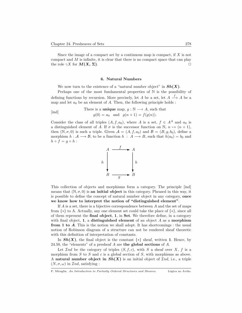
Chapter 24. Presheaves of Sets 278
Since the image of a compact set by a continuous map is compact, if X is notcompact and M is infinite, it is clear that there is no compact space that can playthe role γX for M(X, Σ). 2
6. Natural Numbers
We now turn to the existence of a “natural number object” in Sh(X).
Perhaps one of the most fundamental properties of N is the possibility of
defining functions by recursion. More precisely, let A be a set, let Af−→ A be a
map and let a0 be an element of A. Then, the following principle holds :
[ind]There is a unique map, g : N −→ A, such that
g(0) = a0 and g(n+ 1) = f(g(n)).
Consider the class of all triples (A, f, a0), where A is a set, f ∈ AA and a0 isa distinguished element of A. If σ is the successor function on N, n 7→ (n + 1),then (N, σ, 0) is such a triple. Given A = (A, f, a0) and B = (B, g, b0), define amorphism h : A −→ B, to be a function h : A −→ B, such that h(a0) = b0 andh f = g h :
B
A
?
- A
h
f
B
h
g
?-
This collection of objects and morphisms form a category. The principle [ind]means that (N, σ, 0) is an initial object in this category. Phrased in this way, itis possible to define the concept of natural number object in any category, oncewe know how to interpret the notion of “distinguished element”.
If A is a set, there is a bijective correspondence between A and the set of mapsfrom ∗ to A. Actually, any one element set could take the place of ∗, since allof them represent the final object, 1, in Set. We therefore define, in a categorywith final object, 1, a distinguished element of an object A as a morphismfrom 1 to A. This is the notion we shall adopt. It has shortcomings : the usualnotion of Robinson diagram of a structure can not be rendered sheaf theoreticwith this definition of interpretation of constants.
In Sh(X), the final object is the constant ∗ sheaf, written 1. Hence, by24.50, the “elements” of a presheaf A are the global sections of A.
Let Ind be the category of triples (S, f, c), with S a sheaf over X, f is amorphism from S to S and c is a global section of S, with morphisms as above.A natural number object in Sh(X) is an initial object of Ind, i.e., a triple(N, σ, ω) in Ind, satisfying :
F. Miraglia. An Introduction to Partially Ordered Structures and Sheaves. Logica no Aviao.

Chapter 24. Presheaves of Sets 279
[ind]For all (S, f, c) in Ind, there is a unique g : N −→ S,
such that fX(ω) = c and f g = g σ.
S
N
?
- N
g
σ
S
g
f
?-
Clearly, if it exists, such an object is unique, up to isomorphism.
Theorem 24.66. The triple (NNN, σ, 0), consisting of
∗ The constant N sheaf, NNN;
∗ The ‘successor’ morphism σ, defined, for each u ∈ Ω(X), by
s ∈ NNN(u) 7→ σu(s) = s+ 1;
∗ The global section constantly equal to 0, denoted by 0,
is the natural number object in Sh(X). Furthermore, the following induction prin-ciple holds in NNN : if S is a subsheaf of NNN, the following are equivalent :
(1) S = NNN.
(2) (i) 0 ∈ S(X) (ii) σ(S) ⊆ S.
Proof. Let Q ∈ Sh(X), let q0 ∈ Q(X) be a global section of Q and letµ : Q −→ Q be a morphism. By the classical principle of definition by recursion,there is a unique g : N −→ Q(X), such that g(0) = q0 and g(n+ 1) = µX(g(n)),∀ n ∈ N. By Proposition 24.49.(b), there is a unique morphism λ : NNN −→ Q, suchthat λX(n) = g(n). It is straightforward that λ is the unique morphism from NNN to
Q, such that λX(0) = q0 and λ σ = µ λ, as needed.
For the induction principle, clearly (1) ⇒ (2); for the converse, the conditionsin (2) and the usual induction principle entail that n ∈ |S|, for all n ∈ N. Since
N is dense in NNN (24.46.(a).(2)) and S is a subsheaf of NNN, we obtain S = NNN, asneeded.
We now introduce the sheaf-theoretic counterpart of the familiar structure onNNN. For s, t ∈ |NNN|, define
s + t : Es ∩ Et −→ N by [s + t](x) = s(x) + t(x);
s · t : Es ∩ Et −→ N by [s · t](x) = s(x)t(x),
where the operations in the right-hand side are the usual ones in N. Note that forall a ∈ N,
[(s + t) = a] =⋃b+c=a [[s = b ]] ∩ [[t = c ]]
[(s · t) = a] =⋃bc=a [[s = b ]] ∩ [[t = c ]],
and so s + t, st are, by 24.46.(a), in |NNN|. It is readily verified that addition andproduct are sheaf morphisms from NNN × NNN to NNN.
F. Miraglia. An Introduction to Partially Ordered Structures and Sheaves. Logica no Aviao.
Chapter 24. Presheaves of Sets 280
We also define a binary relation ≤ on NNN by the following prescription, whereu ∈ Ω(X) :
≤(u) = 〈 s, t 〉 ∈ NNN(u) × NNN(u) : ∀ x ∈ u, s(x) ≤ t(x),with restrictions induced by NNN × NNN. The reader can check that ≤ is a subsheaf ofNNN2. We can consider NNN as a structure
NNN = 〈NNN, ≤, +, ·, 0, 1 〉,that has basic properties that are analogous to those found in elementary numbertheory. Although we have not defined the value of formulas in presheaves, we shalldiscuss the interpretation of very simple formulas in NNN, in particular because it isa good introduction to the general case. For instance
(i) ∀s ∀t (s + t = t + s)
expressing the commutativity of addition is true because addition is defined point-wise and it is commutative in N. Similarly, the sheaf operations + and · are commu-tative, associative and have 0 and 1 as neutrals, respectively. Of a slightly differentsort are the properties
(ii) ∀s(s 6= 0 → ∃t(s = t + 1));
(iii) ∀s (s = 0 ∨ ∃t (s = t + 1).
Classically, (ii) and (iii) are equivalent, but not intuitionistically (see 6.8.(h)); ingeneral, we only have (iii) ⇒ (ii). To see that NNN |= (iii), note that, if s ∈ |NNN|, itsextent Es can be partitioned into two disjoint opens :
Es = [[s = 0 ]] ∪ u, where u =⋃n≥1 [[s = n ]]. (*)
In u we may certainly write s as t + 1. Since the union of where the two alternativesin (iii) hold is Es, we consider that NNN |= (iii). For (ii), let s be a section in NNN; the
idea is that in Es (where s exists), if it is distinct from 0, then it must locally bethe successor of a section of NNN, that is
Es ∩ int x ∈ Es : s(x) 6= 0 ⊆⋃t∈|NNN| [[s = (t+ 1)]]. (**)
But this is exactly the content of (*), verifying that NNN |= (ii) 22. In a similar vein,one can prove that ≤ is a linear order on NNN, that is a partial order satisfying
(iv) ∀s ∀t (s ≤ t ∨ t ≤ s).
For, consider
u = x ∈ Es ∩ Et : s(x) ≤ t(x);since s and t are locally constant, for x ∈ u select a clopen v in νx, such thatv ⊆ (Es ∩ Et) and s, t are constant in v. Then v ⊆ u, and so u ∈ Ω(X). A similarreasoning shows that
v = x ∈ Es ∩ Et : t(x) ≤ s(x) ∈ Ω(X).
Since u ∪ v = Es ∩ Et, it follows that NNN models (iv).
Once we have N, there are well known constructions to produce the integers,Z, and the rationals, Q. The proof of this left to the reader as Exercise 24.83
It is also possible to construct the reals in Sh(X). In general however, “com-pletion by Cauchy sequences” gives a different result than “completion by Dedekind
22This can be obtained on general grounds, since, as it shall be seen, sheaves are models for theintuitionistic predicate calculus.
F. Miraglia. An Introduction to Partially Ordered Structures and Sheaves. Logica no Aviao.
Chapter 24. Presheaves of Sets 281
cuts”. The completion by Dedekind cuts of the sheaf QQQ is the sheaf of con-tinuous real valued functions on X, C(X). We refer the interested reader to [55].
If A is a set, a sequence in A is a map f : N −→ A. For presheaves we have
Definition 24.67. If P is a presheaf over X, a sequence in P is a morphismfrom NNN to P .
From 24.49 we get
Corollary 24.68. Let P be a presheaf over X. There is a natural bijectivecorrespondence between sequences in P and (set-theoretical) sequences in P (X).
Exercises
24.69. Determine domain, equality and extent for the initial and final objects0 and 1 (as in 24.1). 2
24.70. Let P --
λ
β
Q be morphisms of presheaves.
a) P ×λ P is the equalizer of P --
λ
λ
Q.
b) Determine the domain, equality and extent of Eq(λ, β), establishing it is anextensional presheaf of sets over X. 2
24.71. Let Pα, α ∈ A, be a family of subpresheaves of P . For u ∈ Ω(X), set
B(u) =⋃α∈A Pα(u),
with restrictions induced by P . Then, B is a presheaf and the join of the Pα inthe complete lattice PP (X). 2
24.72. a) The constant presheaf A over X (23.16) is dense in the constantsheaf A over X.
b) If Pα, α ∈ A, are closed subpresheaves of P , then so is their intersection.Conclude that PP (X) is a complete lattice.
c) Show that PP (X) and PP (X) are closed under the restriction operation definedin Example 23.12. 2
24.73. a) Completion is a functor, c : pSh(X) −→ Sh(X).
b) The functor c preserves monics and epics. 2
24.74. Let P be a presheaf over X and S, T ⊆ |P |.a) S ⊆ T ⇒ S ⊆ T and S ∩ T = S ∩ T .
b) The map (·) : PP (X) −→ PP (X), S 7→ S, is an increasing nucleus on PP (X)(13.1), whose set of fixed points is PP (X). 2
24.75. a) Generalize Lemma 18.17 to pSh(X).
b) Let Pi : i ∈ I be presheaves over X and let P =∏i∈I Pi. For J⊆ I, set
F. Miraglia. An Introduction to Partially Ordered Structures and Sheaves. Logica no Aviao.
Chapter 24. Presheaves of Sets 282
P|J =∏j∈J Pj
and let πJ : P −→ P|J be the projection that forgets the coordinates outside J .
Then, the map
S ∈ PP|J(X) 7→ πJ−1(S) ∈ PP (X),
is a natural bijective correspondence between closed subpresheaves of P|J and
closed subpresheaves of P that depend only on J . A similar statement holds forPP (X) and PP|J(X). 2
24.76. If P is a presheaf over X, the diagonal of Pn,
∆n = (〈 s1, . . . , sn 〉 ∈ |P |n : si = sj , ∀ i, j ≤ n,is a n-ary relation on P . 2
24.77. If R is a relation from P to Q, define domain and image of R. 2
24.78. Let Q be a sheaf over X.
a) The map u ∈ Ω(X) 7→ Q|u ∈ PQ(X) is a frame isomorphism of Ω(X) onto its
image.
b) Is every subsheaf of Q of the form Q|u, for some u ∈ Ω(X) ? 2
24.79. Extend 24.49 to any finite product of constant sheaves. 2
24.80. Every finitely complete C-presheaf is extensional. 2
24.81. Let R1, . . . , Rn be a commutative rings with identity such thatMσ(Ri)is an algebraic frame. If R =
∏ni=1 Ri, then Mσ(R) is a frame 23. 2
24.82. Let N be the natural numbers and Z the ring of integers. Let R = ZN
be the ring of sequences of integers, with its natural coordinate-wise structure.
a) If S ∈ M(Z) and F is a filter on N, then
[F, S] = s ∈ R : n ∈ N : s(n) ∈ S ∈ Fis a multiplicative subset of R, which is saturated if the same is true of S. Moreover
F ⊆ G and S ⊆ T ⇒ [F, S] ⊆ [G,T ].
b) Let F be the filter of cofinite subsets of N and S = U(Z) = ±1. Then, for alln ∈ N, 24
[F, S](n) = s(n) : s ∈ [F, S] = Z.
c) Show that the equivalence in 24.58 is false if X is not compact. 2
24.83. Show that the usual way of introducing the additive inverse in N toconstruct the integers Z, produces, in Sh(X), the constant sheaf ZZZ. Show thatthe “field of fractions” construction, applied to ZZZ, yields the constant sheaf QQQ. 2
23If Ri = R, 1 ≤ i ≤ n, this is an immediate consequence of 24.56.24Notation as in the proof of 24.56.
F. Miraglia. An Introduction to Partially Ordered Structures and Sheaves. Logica no Aviao.
Part 5
L-sets

In this Part we begin the study of an abstract version of sheaves and presheavesthat originated with [26] but developed essentially in [15] and [50]. The symbolL denotes a semilattice (3.1), H stands for a Heyting algebra (6.1), while Ω willbe reserved for a frame (8.1).
Many of the results are generalizations of the ones proven for sheaves andpresheaves over topological spaces. However, since in general HAs do not havepoints, many of the constructions have to be obtained in an intrinsic way. Theproofs of a fair amount of the properties of L-sets are straightforward transcriptionsof those for presheaves of sets over topological spaces.
CHAPTER 25
L-sets and L-presheaves
We start with a general concept of a set with values in a semilattice, obtainedby transcribing to the semilattice context the first two properties in 23.7.(b).
Definition 25.1. Let L be a semilattice. A L-set, A, consists of a set, |A|,(the domain of A), together with a map
[[· = ·]] : |A| × |A| −→ L,
satisfying, for all x, y, z ∈ |A|,[= 1] : [[x = y]] = [[y = x]];
[= 2] : [[x = y]] ∧ [[y = z]] ≤ [[x = z]].
The map [[· = ·]] is the equality relation on A. For x ∈ |A|,Ex =def [[x = x]]
is the extent of x. Clearly, [[x = y]] ≤ Ex ∧ Ey. For S ⊆ |A|, the support ofS is
ES =∨a∈S Ea,
whenever this sup exists in L. When there is need to register explicitly that equality,extent or support refer to A, write [[· = ·]]A and EA.
We refer to an element in |A| as a section of A. For p ∈ L,
A(p) = x ∈ |A| : Ex = p,is the set of sections of A over p. A global section of A is an element of A(>).We shall assume that whenever L has ⊥, any L-set has a unique section over ⊥,indicated by ∗.
A L-set A is extensional iff it satisfies
[ext] For all x, y ∈ |A|, Ex = Ey = [[x = y]] ⇒ x = y.
Unless explicit mention to the contrary, all L-sets are assumed to beextensional.
If A is an L-set and |B| ⊆ |A|, then |B| is the domain of a L-set, obtainedby restricting [[· = ·]] to |B| × |B|. Moreover, if A is extensional, the same will betrue of B; write B ⊆ A to indicate the L-set structure induced by A on |B|.
Example 25.2. Presheaves, P , over a topological space X give rise to a Ω(X)-set, also denoted by P , with |P | =
∐u∈Ω(X) P (u) and for s ∈ P (u), t ∈ P (v),
[[s = t]] =⋃w ∈ Ω(u ∩ v) : s|w = t|w.
By 23.7.(b), this equality relation makes P into a Ω(X)-set. It will be extensionaliff P is an extensional presheaf over X. 2
285
Chapter 25. L-sets and L-presheaves 286
Example 25.3. If A is a L-set and p ∈ L,
|A|p| = x ∈ |A| : Ex ≤ p.is the domain of a L-set A|p, the restriction of A to p. Equality in A|p is induced
by A, i.e., for x, y ∈ |A|p|, [[x = y]]A|p = [[x = y]]A. Clearly, A|p is extensional
whenever the same is true of A. 2
Example 25.4. Let H be a HA. Define an H-set, H, as follows :
∗ |H| = 〈 a, p 〉 ∈ H × H : a ≤ p =⋃p∈H p← × p;
∗ [[〈 a, p 〉 = 〈 b, q 〉]] = p ∧ q ∧ (a ↔ b),
where ↔ is equivalence in H (6.9). By 6.23, this equality satisfies [= 1] and [= 2].
Clearly, E〈 a, p 〉 = p, for all 〈 a, p 〉 ∈ |H|. H corresponds to the sheaf of opens
of a topological space X (23.13). To establish that H is extensional, note thatE〈 a, p 〉 = E〈 b, q 〉 = [[〈 a, p 〉 = 〈 b, q 〉]] entails p = q = p ∧ (a ↔ b). Hence,p ≤ (a ↔ b), and 6.10.(a) yields a = a ∧ p = b ∧ p = b, as needed. 2
Example 25.5. Let L be a semilattice. Define a L-set, 1, by
∗ |1| = L; ∗ [[x = y]] = x ∧ y.
Clearly, 1 is an extensional L-set. 2
Example 25.6. Let R be a commutative ring with identity and let Ω be theframe Rad(R), of radical ideals in R, of Chapter 9, the results of which we shalluse freely. Recall that (x) is the principal ideal generated by x ∈ R. Define a Ω-set,
R, as follows :
∗ |R| = R; ∗ [[a = b]] = (√a ↔
√b) = (
√a :√b) ∩ (
√b :√a).
Recalling that ↔ is the equivalence operation in the frame Ω, it follows from 6.23
that R is a Rad(R)-set, in which every section is global.
R will be extensional iff for all a, b ∈ R√a =√b ⇒ a = b.
Since√
(a2) =√a (the set of primes containing a and a2 are the same), we must
have that a2 = a, for all a ∈ R, that is, R is a Boolean ring. Conversely, if R isa Boolean ring, then
√a =
√b ⇒ a = b. Indeed, by 9.12.(b), the hypothesis
means that there are n, m ≥ 1 such that
an = a ∈ (b) and bm = b ∈ (a).
These relations entail the existence of x, y ∈ R such that a = xb and b = ya;the first of these equations yields ab = xb2 = xb = a, while the second impliesab = ya2 = ya = b, showing that a = b. Hence,
R is an extensional Rad(R)-set iff R is a Boolean ring. 2
Example 25.7. Let R be a commutative regular ring with identity andlet B(R) the BA of idempotents in R (19.19). For a, b ∈ R, there is a uniqueeab ∈ B(R), such that the principal ideal (a − b) is equal to the principal ideal(eab). Hence,
(a− b)eab = (a− b) and eab = αab(a− b), (I)
for some αab ∈ R. Define a B(R)-set, R, as follows :
F. Miraglia. An Introduction to Partially Ordered Structures and Sheaves. Logica no Aviao.
Chapter 25. L-sets and L-presheaves 287
∗ |R| = 〈 a, e 〉 ∈ R × B(R) : ae = a;
∗ [[〈 a, e 〉 = 〈 b, f 〉]]] = (1 − eab)ef .
Clearly, E〈 a, e 〉 = e. One should keep in mind that e·f is e ∧ f in B(R). This con-struction corresponds to the structure sheaf of R over the Boolean space Spec(R)(Example 22.19 and Corollary 22.20). R is extensional, because
E〈 a, e 〉 = E〈 b, f 〉 = [[〈 a, e 〉 = 〈 b, f 〉]],implies e = f = (1− eab)ef ; hence, eabe = 0, and so
a − b = ae − be = e(a − b) = eeab(a − b) = 0,
verifying that a = b, as desired. 2
Example 25.8. This example is an abstract version of the presheaf fA in
23.16. Let A be a set and let L be a distributive lattice, with ⊥ and >. If As−→ L
is a map, the support of s is
spt(s) = a ∈ A : s(a) 6= ⊥.Now define 1
|fA| = s ∈ LA :spt(s) ⊆f A and ∀ a, b ∈ Aa 6= b ⇒ s(a) ∧ s(b) = ⊥.
For s, t ∈ |fA|, set
[[s = t]] =∨a∈A s(a) ∧ t(a).
Note that the join in the definition of [[· = ·]] is finite because the support of s andt are finite. Clearly, [[· = ·]] satisfies [= 1]; for [= 2], we have, using distributivityand the fact that t(a) is disjoint from t(b) for a 6= b,
[[s = t]] ∧ [[t = z]] =∨a∈A s(a) ∧ t(a) ∧
∨a∈A t(a) ∧ z(a)
=∨a,b∈A s(a) ∧ t(a) ∧ t(b) ∧ z(b)
=∨a∈A s(a) ∧ t(a) ∧ z(a)
≤∨a∈A s(a) ∧ z(a) = [[s = z]].
Note that Es =∨a∈A s(a). Hence, fA is a L-set, the bounded constant A
L-set. To see it is extensional, suppose Es = Et = [[s = t]]; for a ∈ A, we have
s(a) = s(a) ∧ Es = s(a) ∧ [[s = t]] = s(a) ∧∨b∈A s(b) ∧ t(b)
=∨b∈A s(a) ∧ s(b) ∧ t(b) = s(a) ∧ t (a),
and so s(a) ≤ t(a). Since the argument is symmetrical in s and t, we conclude thats(a) = t(a), as needed.
To describe the sections in fA that correspond to the constant functions, foreach a ∈ A, define a : A −→ L by
a(b) =
⊥ if a 6= b;
> if b = a.
Then, a is a global section in fA; write A = a : a ∈ A. The map
a ∈ A 7−→ a ∈ fA(>)
is an injection of A into the global sections of fA, with image A.
1Recall (page 15) that ⊆f means “finite subset of”.
F. Miraglia. An Introduction to Partially Ordered Structures and Sheaves. Logica no Aviao.
Chapter 25. L-sets and L-presheaves 288
If L is Ω(X), X a topological space, the construction above is isomorphicto that in Example 23.16. We leave details to the reader, but make the followingobservations :
∗ If f : X −→ A is a continuous map with finite image, define
α(f) : A −→ Ω(X), given by α(f)(a) = [[f = a ]].
Note that α(f) ∈ fA;
∗ If s ∈ |fA|, define β(s) : X −→ A by
β(s)(x) = a iff x ∈ s(a).
Then, β(s) is a continuous map, with finite image in A;
∗ α(β(s)) = s and β(α(f)) = f .
∗ α and β are morphisms of Ω(X)-sets 2. 2
Example 25.9. This example is the abstract counterpart of the constantsheaf presented in 23.17 and discussed in section 24.5.
Let Ω be a frame and A be a set. Let
|A| = s ∈ ΩA : ∀ a, b ∈ A, a 6= b ⇒ s(a) ∧ s(b) = ⊥.Thus, |A| is analogous to |fA|, but without the finiteness assumption on support.For s, t ∈ |A|
[[s = t]] =∨a∈A s(a) ∧ t(a).
As in 25.8
∗ A is an extensional Ω-set, the constant A Ω-set;
∗ The map · : A −→ A ⊆ A(>) is an injection of A into the set of global sectionsof A.
∗ As was the case in 25.8, if Ω is the frame of opens of a topological space, thenthe definition of A given here and that in 23.17 are isomorphic presentations ofthe same object. 2
We now introduce the notion of morphism of L-sets.
Definition 25.10. Let A, B be L-sets. A morphism, Af−→ B, is a set-
theoretical map, f : |A| −→ |B|, such that for all x, y ∈ |A|[mor 1] : EBfx = EAx;
[mor 2] : [[x = y]]A ≤ [[fx = fy]]B.
L-sets and their morphisms form a category, written Lset.
Note that there is no extensionality assumption in 25.10. Moreover, 25.10 isjust a rewriting, with L in place of Ω(X), of item (3) in 23.19 and hence a directdescendant of the corresponding notion for presheaves over a topological space.
25.11. Final and Initial Object. The final object in Lset is the L-set 1of Example 25.5. If A is a L-set, the unique morphism from A to 1 is given bya 7→ Ea. The final object in Lset is the empty L-set, written ∅. Recall that if Lhas ⊥, then |∅| = ∗, with E∗ = ⊥. 2
2Defined in 25.10.
F. Miraglia. An Introduction to Partially Ordered Structures and Sheaves. Logica no Aviao.
Chapter 25. L-sets and L-presheaves 289
25.12. Products. Let A1, . . . , An be L-sets. Define a L-set,∏ni=1 Ai, by the
following rules :
∗ |∏ni=1 Ai| = 〈 a1, . . . , an 〉 ∈
∏ni=1 |Ai| : Ea1 = Ea2 = . . . = Ean;
∗ [[x = y]] =∧ni=1 [[xi = yi]],
where x, y ∈ |∏ni=1Ai|. Note the distinction between the domain of the product
and the product of the domains. Moreover,∏ni=1 Ai is extensional if the same is
true of each coordinate. There are natural morphisms of L-sets
πi :∏ni=1 Ai −→ Ai, πi(a) = ai,
the projections to the ith coordinate. The family
〈∏ni=1 Ai, πi : 1 ≤ i ≤ n 〉
is the product of the Ai in the category Lset. If L is complete lattice, an analogousconstruction shows that Lset has all products. As usual in any category, theempty product is the final object 1. 2
Before going on to describe some of the other standard constructions in thecategory Lset, we set down a vector notation for L-sets, complementing the con-ventions set down in 1.4.
25.13. Notation. Let L be a semilattice and let A1, . . . , An be L-sets. Writex = 〈x1, . . . , xn 〉 for an element of
∏ni=1 |Ai|. For x, y ∈
∏ni=1 |Ai|, define
∗ Ex =∧ni=1 Exi; ∗ [[x = y]] =
∧ni=1 [[xi = yi]].
If L is complete, this notation applies to any family of L-sets. 2
Lemma 25.14. a) If A1, . . . , An are L-sets and a, b, c ∈∏ni=1 Ai, then
(1) [[a = b]] ≤ Ea ∧ Eb; (2) [[a = b]] ∧ [[b = c]] ≤ [[a = c]].
If L is a complete lattice, the above laws hold for any family of L-sets.
b) Let Af−→ B
g−→ C be morphisms of L-sets with h = g f . If L is a completelattice, then for all sets I, a ∈ |A|I and c ∈ |C|I ,
[[ha = c]] =∨b∈|B|I [[fa = b]] ∧ [[gb = c]].
Proof. Item (a) is a straightforward consequence that meets − even infini-tary −, are associative (Lemma 7.7).
b) Fix a ∈ |A|I and c ∈ |C|I ; since g is a morphism, for each b ∈ |B|I and i ∈ I,we have
[[fai = bi]] ≤ [[gfai = gbi]] = [[hai = gbi]],
and so, taking meets over i ∈ I yields [[fa = b]] ≤ [[ha = gb]]. Thus, if b ∈ |B|I
[[fa = b]] ∧ [[gb = c]] ≤ [[ha = gb]] ∧ [[gb = c]] ≤ [[ha = c]],
wherefrom it follows that∨b∈|B|I [[fa = b]] ∧ [[gb = c]] ≤ [[ha = c]].
On the other hand, if we take b = f(a) then∨b∈|B|I [[fa = b]] ∧ [[gb = c]] ≥ [[fa = fa]] ∧ [[gfa = c]]. (1)
Since g is a morphism, one has
F. Miraglia. An Introduction to Partially Ordered Structures and Sheaves. Logica no Aviao.

Chapter 25. L-sets and L-presheaves 290
[[fa = fa]] = Efa = Egfa = Eha.
Thus, item (a) yields
[[fa = fa]] ∧ [[gfa = c]] = Eha ∧ [[ha = c]] = [[ha = c]],
and (1) implies the desired equality.
Recall (25.1) that the support of a L-set A is EA =∨a∈|A| Ea, whenever
this join exists in L. The next result discusses the support of non-empty powersand products 3.
Lemma 25.15. Let L be a complete lattice.
a) A is a L-set and I 6= ∅ is a set, then
EA = EAI =∨a∈|A|I Ea.
b) If Ai, i ∈ I, are L-sets, then
(1) E(Πi∈I Ai) ≤∨c∈Π|Ai| Ec ≤
∧i∈I EAi.
(2) If L is a frame and I is finite, then∨c∈Π|Ai| Ec =
∧i∈I EAi.
Proof. a) The diagonal morphism, ∆ : A −→ AI , ∆(a) = a 4 and 25.36entail EA ≤ EAI . Since |AI | ⊆ |A|I , it suffices to check that
∨a∈|A|I Ea ≤ EA.
But this is clear, because for a ∈∏i∈I |Ai| we have, for some fixed k ∈ I,
Ea =∧i∈I Eai ≤ Eak ≤ EA,
as needed.
b) The inequality in (1) is clear, recalling that |∏i∈I Ai| ⊆
∏i∈I |Ai|. If I is finite
and L is a frame, distributivity of joins over finite meets (8.4) yields, with∧i∈I EAi =
∧i∈I
∨ai∈|Ai| Eai =
∨a∈Π|Ai|
∧i∈I Eai
=∨a∈Π|Ai| Ea.
ending the proof.
Remark 25.16. The reader will easily find examples of Ω-sets A, B such that|A × B| = ∗ 5, but EA ∧ EB 6= ⊥. Hence, the equality between the support ofa product and the meet of the supports of its components is false for Ω-sets, evenfor finite products. For Ω-presheaves, the relation holds for finite products (see26.13); however, even for presheaves, it is false for arbitrary products, as shown in26.14. The same example shows that the equality (2) in 25.15.(b) is also false forinfinite products. 2
25.17. Fibered product over a map. Let f : A −→ B be a morphism inLset. Define a L-set A×f A by the rules :
∗ |A×f A| = 〈x, y 〉 ∈ A × A : fx = fy= 〈 t, z 〉 ∈ |A| × |A| : Ex = Et and ft = fz;
∗ Equality is that induced by A × A.
3The support of the empty product, 1, is >.4The constant I-sequence with entries a.5∗ is the unique section over ⊥ as in 25.1.
F. Miraglia. An Introduction to Partially Ordered Structures and Sheaves. Logica no Aviao.
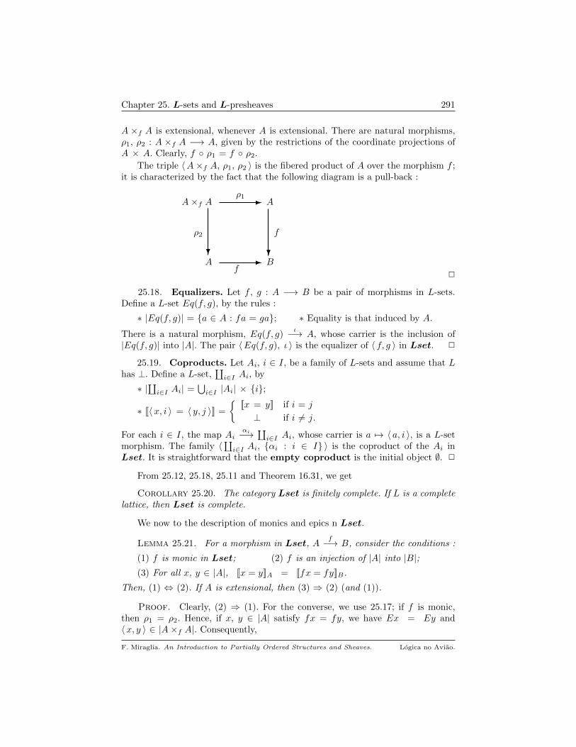
Chapter 25. L-sets and L-presheaves 291
A ×f A is extensional, whenever A is extensional. There are natural morphisms,ρ1, ρ2 : A ×f A −→ A, given by the restrictions of the coordinate projections ofA × A. Clearly, f ρ1 = f ρ2.
The triple 〈A×f A, ρ1, ρ2 〉 is the fibered product of A over the morphism f ;it is characterized by the fact that the following diagram is a pull-back :
A
A×f A
?
- A
ρ2
ρ1
B
f
f
?-
2
25.18. Equalizers. Let f , g : A −→ B be a pair of morphisms in L-sets.Define a L-set Eq(f, g), by the rules :
∗ |Eq(f, g)| = a ∈ A : fa = ga; ∗ Equality is that induced by A.
There is a natural morphism, Eq(f, g)ι−→ A, whose carrier is the inclusion of
|Eq(f, g)| into |A|. The pair 〈Eq(f, g), ι 〉 is the equalizer of 〈 f, g 〉 in Lset. 2
25.19. Coproducts. Let Ai, i ∈ I, be a family of L-sets and assume that Lhas ⊥. Define a L-set,
∐i∈I Ai, by
∗ |∐i∈I Ai| =
⋃i∈I |Ai| × i;
∗ [[〈x, i 〉 = 〈 y, j 〉]] =
[[x = y]] if i = j
⊥ if i 6= j.
For each i ∈ I, the map Aiαi−→
∐i∈I Ai, whose carrier is a 7→ 〈 a, i 〉, is a L-set
morphism. The family 〈∐i∈I Ai, αi : i ∈ I 〉 is the coproduct of the Ai in
Lset. It is straightforward that the empty coproduct is the initial object ∅. 2
From 25.12, 25.18, 25.11 and Theorem 16.31, we get
Corollary 25.20. The category Lset is finitely complete. If L is a completelattice, then Lset is complete.
We now to the description of monics and epics n Lset.
Lemma 25.21. For a morphism in Lset, Af−→ B, consider the conditions :
(1) f is monic in Lset; (2) f is an injection of |A| into |B|;(3) For all x, y ∈ |A|, [[x = y]]A = [[fx = fy]]B.
Then, (1) ⇔ (2). If A is extensional, then (3) ⇒ (2) (and (1)).
Proof. Clearly, (2) ⇒ (1). For the converse, we use 25.17; if f is monic,then ρ1 = ρ2. Hence, if x, y ∈ |A| satisfy fx = fy, we have Ex = Ey and〈x, y 〉 ∈ |A×f A|. Consequently,
F. Miraglia. An Introduction to Partially Ordered Structures and Sheaves. Logica no Aviao.

Chapter 25. L-sets and L-presheaves 292
x = ρ1(〈x, y 〉) = ρ2(〈x, y 〉) = y,
showing that f is an injection. To complete the proof, it is enough to verify that(3) implies (2), when A is extensional. If x, y ∈ |A| are such that fx = fy, then,
[[x = y]] = [[fx = fy]] = Efx = Efy = Ex = Ey,
and extensionality yields x = y, as needed.
By Lemma 25.21, the notion of subobject in Lset is just subset of thedomain, with the induced equality. Hence, the construction described rightafter 25.1, written, A ⊆ B, yields all sub L-sets of B.
The L-set morphism verifying (3) in 25.21 deserve a special name :
Definition 25.22. A L-set morphism Af−→ B is a regular monic if for
all x, y ∈ |A| [[fx = fy]]B = [[x = y]]A.
Lemma 25.23. If f : A −→ B is a morphism of L-sets, the following areequivalent :
(1) f is an isomorphism, i.e., there is a morphism g : B −→ A, such thatg f = IdA and f g = IdB.
(2) f is bijective and a regular monic (25.22).
If A is extensional, these conditions are equivalent to
(3) f is surjective and a regular monic.
Proof. (1) ⇒ (2) : It is enough to check that [[fx = fy]]B ≤ [[x = y]]A. Sinceg f = IdA, the needed inequality amounts to
[[gfx = gfy]]A ≥ [[fx = fy]]B ,
that is a consequence of g being a morphism.
(2) ⇒ (1) : Let g be the (set-theoretical) inverse of f ; thus, for all 〈 a, b 〉 ∈ |A| × |B|,f a = b iff gb = a.
It is immediate that Egb = Eb, for all b ∈ |B|. If b = fa and b′ = fa′, then
[[b = b′]]B = [[fa = fa′]]B = [[a = a′]]A = [[gb = gb′]]A,
verifying that g is a morphism, as needed. To end the proof, just note that, in caseA is extensional, 25.21 guarantees that a regular monic is injective.
The description of epics appears in
Lemma 25.24. Let f : A −→ B be a morphism of L-sets. Assume that L isa frame and consider the following conditions :
(1) f is epic in Lset; (2) ∀ b ∈ |B|, Eb =∨a∈|A| [[b = fa]].
Then, (1) ⇒ (2); if B is extensional, these conditions are equivalent.
Proof. (1) ⇒ (2) : Let L be the L-set of 25.4. We construct two morphisms
h, k : B −→ L, as follows : for b ∈ |B|h(b) = 〈Eb,Eb 〉;k(b) = 〈
∨a∈|A| [[b = fa]], Eb 〉.
F. Miraglia. An Introduction to Partially Ordered Structures and Sheaves. Logica no Aviao.
Chapter 25. L-sets and L-presheaves 293
Note that Ehb = Ekb = Eb; to see that k is indeed a morphism, it is enough toshow that [[b = b′]] ≤ [[kb = kb′]]
= Eb ∧ Eb′ ∧(∨
a∈|A| [[b = fa]] ↔∨a∈|A| [[b′ = fa]]
),
or equivalently (6.10.(a)) that
[[b = b′]] ∧∨a∈|A| [[b = fa]] = [[b = b′]] ∧
∨a∈|A| [[b = fa]]. (I)
Since L is a frame, we have
[[b = b′]] ∧∨a∈|A| [[b = fa]] =
∨a∈|A| [[b = b′]] ∧ [[b = fa]]
≤∨a∈|A| [[b′ = fa]].
By symmetry, we obtain the equality in (I), as needed. The verification that h isalso a morphism is straightforward. Now observe that for all a ∈ |A|
k(fa) = 〈∨a′∈|A| [[fa = fa′]], Efa 〉 = 〈Efa,Efa 〉 = h(fa),
and so h f = k f . Since f is epic, we conclude that h = k, establishing theequality in (2) for all b ∈ B.
(2) ⇒ (1) : Assume that B is extensional and let B --
h
k
C be morphisms,
such that f h = f k. For b ∈ |B|, the transitivity of equality ([= 2] in 25.1)yields, with a ∈ |A|[[hb = kb]] ≥ [[hb = hfa]] ∧ [[hfa = kb]] = [[hb = hfa]] ∧ [[kfa = kb]]
≥ [[b = fa]] ∧ [[fa = b]] = [[b = fa]]. (II)
Hence, taking joins over a ∈ |A| in (II) yields
[[hb = kb]] ≥∨a∈|A| [[b = fa]] = Eb,
and extensionality entails hb = kb, concluding the proof.
The notions of compatibility and of “gluing” compatible families is at the heartof sheaf theory. We shall discuss these notions in the context of L-sets, indicatingthe need for L to satisfy a [∧,
∨]- law (8.6) in order to have a smooth theory of
sheaves and presheaves.
Let A be L-set, with L a semilattice. How would we define compatibility ofsections in |A| ? Given x ∈ |A|, we think of Ex as the largest element of L wherex exists. Equality, is thought of as the largest element of L over which x and ycoincide. Thus, two sections x, y of A should be compatible if and only if the valueof their equality is the intersection of their extents. Hence,
Definition 25.25. A set of sections S ⊆ |A| in a L-set A is compatible ifffor all s, t ∈ S Es ∧ Et = [[s = t]].
Next, what would be the right concept of “gluing” ? We wish to find, given acompatible S ⊆ |A|, a section t ∈ |A| that “extends” all s ∈ S. Consequently, tmust have extent, at least
∨s∈S Es; in particular, we must assume that this sup
exists in L. Secondly, it is expected that in each Es, t and s coincide. Since thereis no information about t outside
∨s∈S Es, we are led to require that t satisfy
F. Miraglia. An Introduction to Partially Ordered Structures and Sheaves. Logica no Aviao.
Chapter 25. L-sets and L-presheaves 294
[gl >]
(i) Et =
∨s∈S Es
(ii) For all s ∈ S, Es = [[t = s]].
Note that if t and t′ satisfy (i) and (ii) in [gl >], then, for s ∈ S,
[[t = t′]] ≥ [[t = s]] ∧ [[t′ = s]] = Es ∧ Es = Es,
and so [[t = t′]] ≥∨s∈S Es = Et = Et′. Hence, extensionality implies
uniqueness of a section satisfying [gl >]. All seems to be working fine, even in thegeneral context of semilattices. It is a different matter when we try to localize theabove reasoning.
Definition 25.26. Let L be a semilattice and p ∈ L. A set of sections S ina L-set A is compatible over p iff for all s, t ∈ S,
p ∧ Es ∧ Es = p ∧ [[s = t]]. 6
If S is compatible over p ∈ L, one expects to be able to glue, uniquely, thepieces of elements of S that lie over p. To each s ∈ S, there corresponds a pieceof s over p − which may not be in |A| −, but whose extent ought to be p ∧ Es.Hence, by analogy with [gl >], if
∨s∈S p ∧ Es exists in L, we are looking for t ∈
|A|, such that
[gl p]∗
(i) Et =
∨s∈S p ∧ Es;
(ii) For all s ∈ S, p ∧ Es = p ∧ [[t = s]].
If t and t′ satisfy [gl p]∗, then, for s ∈ S,
[[t = t′]] ≥ [[t = s]] ∧ [[s = t′]] = p ∧ Es,and so, [[t = ′t′]] ≥
∨s∈S p ∧ Es = Et = Et′, and extensionality again
entails the desired uniqueness.
But there is another plausible alternative for the extent condition (i) in [gl p]∗:Et = p ∧
∨s∈S Es. After all, we have information to determine t in the inter-
section of p and∨s∈S Es, assuming, of course, that this join exists in L. Since L
does not necessarily satisfy the [∧,∨
]-law of 8.6, we may have
p ∧∨s∈S Es >
∨s∈S p ∧ Es,
with a (possibly) significant difference between these terms. Requiring that theextent of the gluing be the largest it can be is coded by
[gl p]∗
(i) Et = p ∧
∨s∈S Es;
(ii) For all s ∈ S, p ∧ Es = p ∧ [[t = s]].
Perhaps a fruitful analogy is with integration : condition [gl p]∗ yields a “lowergluing”, while [gl p]∗ defines an “upper gluing” of S over p. In general, uppergluings are not unique :
Example 25.27. Let L be the complete (non-distributive) lattice of Remark5.2 :
6Thus, compatibility (25.25) corresponds to the case p = > in the present definition.
F. Miraglia. An Introduction to Partially Ordered Structures and Sheaves. Logica no Aviao.
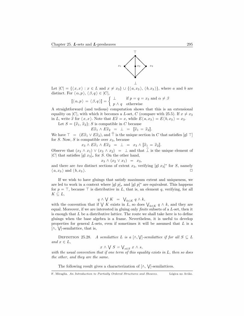
Chapter 25. L-sets and L-presheaves 295
>•
x1 x2• x3
• @@@
•
•⊥
@@@
Let |C| = 〈x, x 〉 : x ∈ L and x 6= x3 ∪ 〈 a, x3 〉, 〈 b, x3 〉, where a and b aredistinct. For 〈α, p 〉, 〈β, q 〉 ∈ |C|,
[[〈α, p 〉 = 〈β, q 〉]] =
⊥ if p = q = x3 and α 6= β
p ∧ q otherwise
A straightforward (and tedious) computation shows that this is an extensionalequality on |C|, with which it becomes a L-set, C (compare with 25.5). If x 6= x3
in L, write x for 〈x, x 〉. Note that Ex = x, while E〈 a, x3 〉 = E〈 b, x3 〉 = x3.
Let S = x1, x2; S is compatible in C because
Ex1 ∧ Ex2 = ⊥ = [[x1 = x2]].
We have > = (Ex1 ∨ Ex2), and > is the unique section in C that satisfies [gl >]for S. Now, S is compatible over x3, because
x3 ∧ Ex1 ∧ Ex2 = ⊥ = x3 ∧ [[x1 = x2]].
Observe that (x3 ∧ x1) ∨ (x3 ∧ x2) = ⊥ and that ⊥ is the unique element of|C| that satisfies [gl x3]∗ for S. On the other hand,
x3 ∧ (x2 ∨ x1) = x3,
and there are two distinct sections of extent x3, verifying [gl x3]∗ for S, namely〈 a, x3 〉 and 〈 b, x3 〉. 2
If we wish to have gluings that satisfy maximum extent and uniqueness, weare led to work in a context where [gl p]∗ and [gl p]∗ are equivalent. This happensfor p = >, because > is distributive in L, that is, an element q, verifying, for allK ⊆ L,
q ∧∨K =
∨k∈K q ∧ k,
with the convention that if∨K exists in L, so does
∨k∈K q ∧ k, and they are
equal. Moreover, if we are interested in gluing only finite subsets of a L-set, then itis enough that L be a distributive lattice. The route we shall take here is to definegluings when the base algebra is a frame. Nevertheless, it is useful to developproperties for general L-sets, even if sometimes it will be assumed that L is a[∧,∨
]-semilattice, that is,
Definition 25.28. A semilattice L is a [∧,∨
]-semilattice if for all S ⊆ Land x ∈ L,
x ∧∨S =
∨s∈S x ∧ s,
with the usual convention that if one term of this equality exists in L, then so doesthe other, and they are the same.
The following result gives a characterization of [∧,∨
]-semilattices.
F. Miraglia. An Introduction to Partially Ordered Structures and Sheaves. Logica no Aviao.
Chapter 25. L-sets and L-presheaves 296
Proposition 25.29. Let L be a semilattice with ⊥ and >. The following areequivalent :
(1) L is a [∧,∨
]-semilattice. (2) L can be regularly embedded in a frame.
Proof. The definition of regular embedding appears in 7.3. By 8.7, (2) im-plies (1). For the converse, the reader can verify that Definition 14.1, as wellas the proofs of Lemma 14.2 and Theorem 14.4 apply, verbatim, to a [∧,
∨]-
semilattice.
The hypothesis of regular in 25.29.(2) cannot be omitted, for the completelattice L in 25.27 can be embedded, as a semilattice, into a complete Booleanalgebra.
By 8.7, HAs and BAs are [∧,∨
]-semilattices; moreover, a complete [∧,∨
]-semilattice is a frame. Thus, there is enough variety in structure to sample impor-tant constructions. We formally set down 7
Definition 25.30. Let A be an Ω-set, S ∪ t ⊆ |A| and p ∈ Ω. The sectiont is a gluing of S over p if the following conditions are satisfied
[glu p]
(i) Et = p ∧
∨s∈S Es;
(ii) For all s ∈ S, p ∧ Es = [[t = s]],
When p = >, t is a gluing of S in A.
The next result shows that equality of gluings is determined by the equalityof the pieces being glued.
Lemma 25.31. Let A be a Ω-set and x, y be sections in A, that are gluingsover p ∈ Ω of S, T ⊆ |A|, respectively. Then,
p ∧ [[x = y]] = p ∧∨〈s,t〉∈S×T [[s = t]].
Proof. We shall treat the case in which p = >, leaving the straightforwardgeneralization to the reader. By 25.30, we have
(i) Ex =∨s∈S Es;
(ii) ∀ s ∈ S, Es = [[x = s]];
(iii) Ey =∨t∈t Et;
(iv) ∀ t ∈ t, Et = [[y = t]];(*)
The equations in (*), the distributive law in 8.4 and Exercise 25.35 yield
[[x = y]] = [[x = y]] ∧ Ex ∧ Ey = [[x = y]] ∧∨s∈S Es ∧
∨t∈T Et
=∨〈s,t〉∈S×T [[x = y]] ∧ Es ∧ Et
=∨〈s,t〉∈S×T [[x = y]] ∧ [[x = s]] ∧ [[y = t]]
=∨〈s,t〉∈S×T [[s = t]] ∧ [[x = s]] ∧ [[y = t]]
=∨〈s,t〉∈S×T [[s = t]] ∧ Es ∧ Et
=∨〈s,t〉∈S×T [[s = t]],
as desired.
Another concept that can be conveniently treated when the base is a frame isdenseness.
7Recall our standing convention that L is a semilattice, H is a HA and Ω a frame.
F. Miraglia. An Introduction to Partially Ordered Structures and Sheaves. Logica no Aviao.
Chapter 25. L-sets and L-presheaves 297
Definition 25.32. Let A be a Ω-set and S, T ⊆ |A|.
a) S is dense in T if for all t ∈ T , Et =∨s∈S [[s = t]].
b) The density of A, d(A), is the least cardinal γ such that there is dense subsetof A of cardinal γ. A is separable if d(A) is at most countable.
Lemma 25.33. Let A be a Ω-set and D be a dense set of sections in A. LetB be an extensional Ω-set.
a) The relation of being dense is transitive.
b) If a, b ∈ |A|, then [[a = b]] =∨d,d′∈D [[d = d′]] ∧ [[a = d]] ∧ [[b = d′]].
c) If f , g : A −→ B are morphisms of Ω-sets, then f|D = g|D ⇒ f = g.
c) A morphism Af−→ B is epic iff f(A) is dense in B.
Proof. a) If S is dense in T , T is dense in X and x ∈ X, then
Ex =∨t∈T [[x = t]] =
∨t∈T [[x = t]] ∧ Et
=∨t∈T [[x = t]] ∧
(∨s∈S [[t = s]]
)=
∨s∈S
∨t∈T [[x = t]] ∧ [[t = s]]
≤∨s∈S [[x = s]] ≤ Ex,
establishing that S is dense in X.
b) As in the proof of 25.31, if a, b ∈ |A|, then 25.35 yields
[[a = b]] = [[a = b]] ∧ Ea ∧ Eb= [[a = b]] ∧
∨d∈D [[a = d]] ∧
∨d′∈D [[b = d′]]
=∨d,d′∈D [[a = b]] ∧ [[a = d]] ∧ [[b = d′]]
=∨d,d′∈D [[d = d′]] ∧ [[a = d]] ∧ [[b = d′]],
as needed.
c) For a ∈ A and d ∈ D, we have
[[fa = ga]] ≥ [[fa = fd]] ∧ [[fd = ga]] = [[fa = fd]] ∧ [[gd = ga]]
≥ [[a = d]],
and so taking joins over d ∈ D, we arrive at [[fa = ga]] ≥ Ea. Since B is exten-sional, we conclude that fa = ga, as desired. Item (c) is just a rephrasing of theequivalence in 25.24.
We end this section with the concept of finite completeness.
Definition 25.34. Let L be a distributive lattice. A L-set A is finitely com-plete (fc) if for all p ∈ L and S ⊆f |A|, if S is compatible over p, then there isa unique t ∈ |A| such that
Et = p ∧∨s∈S E s and p ∧ Es = [[t = s]], ∀ s ∈ S.
F. Miraglia. An Introduction to Partially Ordered Structures and Sheaves. Logica no Aviao.
Chapter 25. L-sets and L-presheaves 298
Exercises
25.35. If A is a L-set and a, b, x, y ∈ |A|, then the following exchange ruleshold true :
a) [[a = b]] ∧ [[a = x]] ∧ [[b = y]] = [[x = y]] ∧ [[a = x]] ∧ [[b = y]].
b) [[x = b]] ∧ [[x = a]] = [[a = b]] ∧ [[x = a]]. 2
25.36. If A, B are L-sets such that EA, EB ∈ L (25.1) and there is a morphismfrom A to B, then EA ≤ EB. 2
25.37. If L is a semilattice, p ∈ L and I is a finite set,
(1|p)I ≈ 1|p.
The same is true for any set I whenever L is complete. 2
25.38. Let A, B be Ω-sets, S ⊆ |A| and p ∈ Ω. Let f : A −→ B be amorphism of Ω-sets.
a) If S has a gluing over p, then S is compatible over p.
b) If A is extensional, then gluings are unique (whenever they exist).
c) If S is compatible over p in A, then f(S) = fs : s ∈ S is compatible over pin B.
d) If t is a gluing of S over p in A, then ft is a gluing of f(S) over p in B. 2
25.39. a) H(>) is dense in H (25.4).
b) A is dense in fA (25.8) and in A (25.9).
c) There are separable Ω-sets with domain of arbitrarily large cardinality. 2
25.40. a) fA is finitely complete.
b) If H is a HA, H (25.4) is finitely complete.
c) Show that the categorical constructions discussed in this Chapter lead fromfc-sets to fc-sets.
d) Determine which of the Examples of this Chapter are finitely complete. 2
F. Miraglia. An Introduction to Partially Ordered Structures and Sheaves. Logica no Aviao.
CHAPTER 26
Presheaves over a Semilattice
As was the case with L-sets, the definition of a presheaf over a semilattice isobtained by specifying [rest 1] through [rest 3] in 23.7.(a) as axioms :
Definition 26.1. Let L be a semilattice.
a) A presheaf P over L 1 is a set |P | (the domain of P ), together with maps
E : |P | −→ L (extent) and
| : |P | × L −→ |P |
〈 a, p 〉 7→ a|p(restriction)
satisfying, for all a ∈ |P |, p, q ∈ L[rest 1] : a|Ea = a; [rest 2] : Ea|p = Ea ∧ p;
[rest 3] : (a|p)|q = a|p∧q.
b) For q ∈ L, P (q) = a ∈ |P | : Ea = q is the set of sections of P overq; an element of P (>) is called a global section of P .
Whenever L has ⊥, we assume that any presheaf over L has a unique sectionover ⊥, written ∗ (as for L-sets).
c) For p ∈ L and S ⊆ |P |,∗ ES =
∨a∈A Ea is the support of S in P , whenever this join exists in L;
∗ S is compatible over p iff for all x, y ∈ S, x|p∧Ex∧Ey = y|p∧Ex∧Ey.
∗ S is compatible if x|Ex∧Ey = y|Ex∧Ey, for all x, y ∈ S.
d) If S ⊆ |P | and t ∈ |P |, t is a gluing of S in P if
Et =∨s∈S Es and t|Es = s, ∀ s ∈ S.
e) A presheaf P over L is extensional if for all x, y ∈ |P | and D ⊆ L
[ext] ∀ p ∈ D, x|p = y|p and Ex = Ey =∨D ⇒ x = y.
f) If P and Q are L-presheaves, a map f : |P | −→ |Q| is a morphism iff for allx ∈ |P | and p ∈ L
[pmor 1] : Efx = Ex [pmor 2] : f(x|p) = (fx)|p.
Write pSh(L) for the category of L-presheaves and their morphisms.
1Or L-presheaf.
299
Chapter 26. Presheaves over a Semilattice 300
As for L-sets (25.36), the support of the source of a morphism is less than orequal to the support of its target.
By Proposition 23.7, every presheaf over a topological space X gives rise toa Ω(X)-presheaf, with same domain and restriction, which is extensional iff theoriginal presheaf is extensional. Moreover, by 23.19, a morphism of presheaves overX gives rise to a morphism of Ω(X)-presheaves. In fact, we have
Lemma 26.2. The categories pSh(X) and pSh(Ω(X)) are isomorphic,the same being true of the corresponding extensional subcategories.
Proof. We only comment in how a Ω(X)-presheaf P gives rise to a presheafover X. If u ≤ v, the restriction map of P yields a map
pvu : P (u) −→ P (v), pvu(s) = s|v,which satisfies puu = IdP (u) (by [rest 1]) and pvu pwv = pwu, if u ≤ v ≤ w(by [rest 3]); that morphisms correspond bijectively follows from 23.19.(c).
Because of 26.2, we shall not distinguish between the categories of Ω(X)-presheaves and presheaves over X.
Exercise 26.23 collects some of basic properties of L-presheaves and their mor-phisms, entirely analogous to the ones for presheaves over topological spaces. Theconcept of [∧,
∨]-semilattice is defined in 25.28.
Example 26.3. Let 2 = ⊥, >; a 2-presheaf can be naturally identifiedwith its set of global sections; and morphisms identified with the induced map onglobal sections. Hence, the categories pSh(2) and Set are naturally isomorphicand Sheaf Theory can be considered as a generalization of Set Theory. 2
Example 26.4. Let A be a set and L a semilattice. We construct a L-presheaf,also written A, as follows :
(i) |A| =⋃⊥6=p∈L A × p ∪ 〈 ∗,⊥〉; (ii) E〈x, p 〉 = p;
(iii) 〈x, p 〉|q = 〈x, p ∧ q 〉.
A is the constant presheaf on L. If f : A −→ B is a map, f induces a morphismof L-presheaves,
〈x, p 〉 7−→
〈 fx, p 〉 if p 6= ⊥〈 ∗,⊥〉 if p = ⊥,
still indicated by f . It is straightforward that these definitions yield a functor fromSet to pSh(L), the constant presheaf functor. 2
Example 26.5. Let L ⊆ R be semilattices and let A be a R-presheaf. Wedefine a L-presheaf, A|L, the restriction of A to L, by the following rules :
i) |A|L| =∐p∈R A(p);
ii) Extent and restriction are those induced by A.
Note that for p, q ∈ L and x ∈ A(p), we have
x|q = x|p∧q ∈ A(p ∧ q) ⊆ |A|L|,
F. Miraglia. An Introduction to Partially Ordered Structures and Sheaves. Logica no Aviao.
Chapter 26. Presheaves over a Semilattice 301
and A|L is indeed a L-presheaf. Clearly, A|L is extensional whenever the same is
true of A. If L = p←, p ∈ R, write A|p for the restriction of A to p←. Note that
|A|p| = x ∈ |A| : Ex ≤ p,as was the case for L-sets in 25.3. There is a natural injection
rA : A|L −→ A, given by x ∈ |A|L| 7−→ x ∈ |A|,such that for all p ∈ L and x ∈ |A|L|, rA(x|p) = (rAx)|p. 2
Before giving more examples, we establish a connection between L-presheavesand L-sets, starting with the following
Definition 26.6. Let L be a semilattice and let A be a L-set which is also aL-presheaf. The equality and restriction in A are compatible if for all x, y ∈ |A|and all p, q ∈ L
(i) Ex = [[x = x]]; (ii) [[x|p = y|q]] = p ∧ q ∧ [[x = y]],
where in (i), Ex is the extent map that comes with the L-presheaf structure of A.
Lemma 26.7. Let L be a semilattice and let A be a L-presheaf with a compatiblestructure of L-set.
a) For x ∈ |A| and p ∈ L, Ex|p = [[x|p = x]] = p ∧ Ex. If A is an extensional
L-set, then x|p is the unique element t ∈ |A| satisfying Et = [[t = x]] = p ∧ Ex.
b) If A is an extensional L-set, then A is an extensional presheaf.
c) Let B be an extensional L-set with a compatible structure of L-presheaf. Thenevery L-set morphism from A to B is a presheaf morphism.
Proof. a) The definition of L-presheaf entails Ex|p = p ∧ Ex; on the other
hand, (i) and (ii) in 26.6 yield [[x|p = x]] = p ∧ Ex, as desired. The remaining
statement is clear.
b) Suppose x, y ∈ |A| and there is D ⊆ L such that∨D = Ex = Ey and x|p = y|p,
for all p ∈ D. Transitivity of equality and (a) yield, for p ∈ D,
[[x = y]] ≥ [[x = x|p]] ∧ [[x|p = y]] = p ∧ Ex ∧ [[y|p = y]]
= p ∧ Ex ∧ Ey = p,
and so [[x = y]] ≥∨D = Ex = Ey. Hence, extensionality entails x = y, as needed.
c) It must be shown that if x ∈ |A| and p ∈ L, then f(x|p) = (fx)|p. Since f is a
morphism, item (a) yields ∗ Ef(x|p) = Ex|p = p ∧ Ex = E(fx)|p;
∗ p ∧ Ex = [[x|p = x]] ≤ [[f(x|p) = fx]] ≤ Ef(x|p) = p ∧ Ex,
and the extensionality of B implies f(x|p) = (fx)|p, as desired.
The next result guarantees a large supply of presheaves with a compatibleequality.
F. Miraglia. An Introduction to Partially Ordered Structures and Sheaves. Logica no Aviao.

Chapter 26. Presheaves over a Semilattice 302
Theorem 26.8. Let P be a presheaf over a subsemilattice L of a frame Ω.For x, y ∈ |P |, set
[equ] [[x = y]] =∨p ∈ L : p ≤ Ex ∧ Ey and x|p = y|p,
where this join is computed in Ω. Then, for x, y ∈ |A| and p, q ∈ La) [[x = y]] is an equality in |P |, with which it becomes a Ω-set, called the Ω-set associated to the presheaf P , still indicated by P . Furthermore, P is anextensional Ω-set iff P is an extensional presheaf over L.
b) [[x|p = y|q]] = p ∧ q ∧ [[x = y]].
c) Ex|p = [[x|p = x]] = p ∧ Ex. If P is extensional, x|p is the unique t in
|P | such that Et = [[t = x]] = p ∧ Ex.
d) If P is extensional, then
(1) x|p = y|p iff p ≤ (Ex ∨ Ey) → [[x = y]] 2.
(2) If p ≤ Ex ∧ Ey, then x|p = y|p iff p ≤ [[x = y]].
(3) If [[x = y]] ∈ L, then x|[[x=y]]= y|[[x=y]]
.
e) Let P and Q be presheaves over L and let f : |P | −→ |Q| be a map. Considerthe following conditions :
(1) f is a presheaf morphism. (2) f is a Ω-set morphism.
Then, (1) ⇒ (2) and they are equivalent if Q is extensional.
Proof. Throughout the proof, write
Exy = p ∈ L : p ≤ Ex ∧ Ey and x|p = y|p,where x, y ∈ |P |. Hence, [[x = y]] =
∨Exy. For q ∈ L, let
q ∧ Exy = q ∧ p : p ∈ Exy.a) It is clear that [[x = x]] = Ex and that [[x = y]] = [[y = x]]. For transitivity, ifp ∈ Exy and q ∈ Eyz, note that (p ∧ q) ≤ Ex ∧ Ez and
x|p∧q = (x|p)|q = (y|p)|q = y|p∧q,that is, p ∧ q ∈ Exz. Hence,
p ∧ q : p ∈ Exy and q ∈ Eyz ⊆ Exz. (*)
Now, (*) and 8.4 immediately imply [[x = y]] ∧ [[y = z]] ≤ [[x = z]], as desired. Itis straightforward that P is an extensional Ω-set iff it is an extensional L-presheaf.
b) Write s = x|p and t = y|q; since Es = p ∧ Ex and Et = q ∧ Ey, if r ∈ Est,then
Er ≤ p ∧ q ∧ Ex ∧ Ey and
x|r = x|p∧r = (x|p)|r = s|r = t|r = (y|q)|r = y|q∧r = y|r,wherefrom we conclude that r ∈ Exy. Consequently,
[[x|p = y|q]] ≤ p ∧ q ∧ [[x = y]].
2∨ and → are join and implication in Ω.
F. Miraglia. An Introduction to Partially Ordered Structures and Sheaves. Logica no Aviao.
Chapter 26. Presheaves over a Semilattice 303
To prove the reverse inequality, it is enough to verify, because Ω is a frame, thatif u ∈ Exy, then p ∧ q ∧ u ∈ Est. We have,
s|p∧q∧u = (x|p)|p∧q∧u = x|p∧q∧u = (x|u)|p∧q = (y|u)|p∧q = y|p∧q∧u= (y|q)|p∧q∧u = t|p∧q∧u,
completing the proof of (b); item (c) follows from (b), as in 26.7.(a).
d) Suppose that p ≤ (Ex ∨ Ey) → [[x = y]], that is (by [→] in 6.1)
p ∧ (Ex ∨ Ey) ≤ [[x = y]] ≤ Ex ∧ Ey.
The above inequalities entail p ∧ Ex = p ∧ Ey = p ∧ Ex ∧ Ey and hence,
p ∧ Ex = Ex|p = p ∧ Ey = Ey|p = p ∧ [[x = y]].
Consider the set D = p ∧ Exy; Ω being a frame, we have∨D = p ∧
∨Exy = p ∧ [[x = y]] = p ∧ Ex = p ∧ Ey.
Since L is a subsemilattice of Ω, p ∧ Exy ⊆ L and p ∧ Ex ∈ L, it follows that∨D
exists in L and is equal to p ∧ Ex = p ∧ Ey. Because x|q = y|q, for all q ∈ Exy,
it follows that for all r = (p ∧ q) in D, we have
x|r = x|p∧q = (x|q)|p = (y|q)|p = y|p∧q = y|r,and extensionality implies x|p = y|p. Conversely, suppose that x|p = y|p. By item
(b),
Ex|p = p ∧ Ex = p ∧ Ey = Ey|p = [[x|p = y|p]] = p ∧ [[x = y]].
Hence, p ∧ (Ex ∨ Ey) = p ∧ Ex = p ∧ [[x = y]] ≤ [[x = y]], as needed. Items(2) and (3) in (d) follow straightforwardly from what has already been proven.
e) Let f : |P | −→ |Q| be a map and assume that f is the carrier of a presheafmorphism. For x, y ∈ |P |, if p ∈ Exy, [pmor 2] implies that p ∈ Efx,fy; hence,[[x = y]] ≤ [[fx = fy]]. Since extent is the same for a presheaf over L and forthe associated Ω-set, we conclude that f is the carrier of a morphism of Ω-sets.The proof of the converse is analogous to that of 26.7.(c).
Remark 26.9. If L is a subsemilattice of a frame and A is a L-presheaf, A willalways be considered as an Ω-set with the equality in 26.8 (the Ω-set associatedto A). In particular, every Ω-presheaf gives rise to a Ω-set, indicated by the samesymbol. Without explicit mention to the contrary, all L-set concepts used for aL-presheaf A, refer to the equality in 26.8. 2
Example 26.10. All the examples in Chapter 25, except 25.3 and 25.6, can begiven a compatible structure of extensional presheaf, as follows (numbering refersto the original example) :
25.4. For 〈 a, p 〉 ∈ |H| and q ∈ H, the rules
E〈 a, p 〉 = p and 〈 a, p 〉|q = 〈 a ∧ q, p ∧ q 〉,
make |H| a presheaf over H. Now suppose that 〈 a, p 〉 and 〈 b, p 〉 are sections in
H, such that there is pi ∈ H satisfying p =∨i∈I pi and
F. Miraglia. An Introduction to Partially Ordered Structures and Sheaves. Logica no Aviao.
Chapter 26. Presheaves over a Semilattice 304
〈 a, p 〉|pi= 〈 a ∧ pi, p ∧ pi 〉 = 〈 b ∧ pi, p ∧ pi 〉.
Then, for all i ∈ I, a ∧ pi = b ∧ pi, that is, pi ≤ (a ↔ b). Hence, p ≤ (a ↔ b),
and so, a = a ∧ p = b ∧ p = b, showing that, as a presheaf, H satisfies [ext].
25.5. For p, q ∈ L, set Ep = p and p|q = p ∧ q; extensionality is clear.
25.7. Let R be a commutative regular ring and let B(R) the BA of idempotentsin R. For 〈 a, e 〉 ∈ |cR| and f ∈ B(R), set
E〈 a, e 〉 = e and 〈 a, e 〉|f = 〈 af, ef 〉.
Then, R is a B(R)-presheaf. To see that it is extensional, assume that 〈 a, e 〉,〈 b, e 〉 ∈ |R| are such that there are fi ∈ B(R), with∨
i∈I fi = e and fi(a− b) = 0, for all i ∈ I.
It follows from (I) in 25.7, that eabfi = 0, for all i ∈ I. Since B(R) is a Booleanalgebra, it is a [∧,
∨]-lattice (8.7) and so,
eabe = eab ∧∨i∈I fi =
∨i∈I eabfi = 0.
But then, again by (I) in 25.7, we get
a− b = eab(a− b) = eab(ae− be) = eabe(a− b) = 0,
as needed to show that R is an extensional presheaf.
25.8. For s ∈ |fA| and p ∈ L, set Es =∨a∈A s(a). Now define
s|p : A −→ L by s|p(a) = p ∧ s(a).
It is clear that spt(s|p) ⊆ spt(s), being therefore finite in A. These definitions make
fA into an extensional L-presheaf. The proof of extensionality is essentially thesame as that given in 25.8. The same technique will show that the constant Ω-setA is a Ω-presheaf.
25.27. Recall that |A| = x1, x2, >, ⊥, 〈 a, x3 〉, 〈 b, x3 〉. Define
∗ Ex = x, if x 6= x3, and E〈 a, x3 〉 = E〈 b, x3 〉 = x3;
∗ 〈α, p 〉|q =
〈α, p 〉 if p ≤ q
⊥ if p ∧ q = ⊥x if α = p = > and q 6= x3
〈 a, x3 〉 if α = p = > and q = x3,
yielding extent and restriction that verify the conditions in 26.1. Since > is the onlyelement of L with a non-trivial cover, and A(>) is a singleton, A is extensional. 2
To describe some of the usual categorical constructions in pSh(L), we intro-duce a vector notation, complementing 25.13 :
26.11. Notation. Let A1, . . . , An be L-presheaves. If x ∈∏ni=1 |Ai| and
p ∈ L, set
∗ Ex =∧ni=1 Exi; ∗ x|p = 〈xi|p 〉.
If L is complete, this notation applies to any family of presheaves over L. 2
F. Miraglia. An Introduction to Partially Ordered Structures and Sheaves. Logica no Aviao.
Chapter 26. Presheaves over a Semilattice 305
26.12. Products. Let Ai, i ∈ I, be L-presheaves. Let
|∏i∈I Ai| = x ∈
∏i∈I |Ai| : ∀ i, j ∈ I, Exi = Exj.
Define extent and restriction in∏i∈I Ai by
x 7−→ Ex and 〈x, p 〉 7−→ x|p,where p ∈ L. Then,
∏i∈I Ai is a L-presheaf, which is extensional iff the same is
true of each coordinate. There are maps
πi :∏i∈I Ai −→ Ai, πi(x) = xi,
which are morphisms of presheaves, called the projections on the ith coordinate.The family 〈
∏i∈IAi, πi : i ∈ I 〉 is the product of the Ai in pSh(L). 2
Lemma 26.13. If A1, . . . , An are Ω-presheaves then
E(Πni=1 An) =
∨a∈Π|Ai| Ea =
∧ni=1 EAi.
Proof. The second equality follows from 25.15.(b).(2). Set P =∏i∈I Ai.
Note that for a ∈∏i∈I |Ai|, 26.8.(c) yields
Ea = Ea|Ea and a|Ea ∈ |P |.Thus, EP ≥
∨a∈Π|Ai| Ea, and so equality follows from (1) and (2) in 25.15.(b).
Example 26.14. We shall construct a sequence An of presheaves, such that
EAn = > but E(∏
n≥1 An
)= ⊥. Let B be the BA of clopens in the Cantor space
2N. As in Chapter 18, for n ≥ 1 and s ∈ 2n, Vs = t ∈ 2N : t|n = s. Moreover,
for each n ≥ 1,⋃s∈2n Vs = 2N, the top of the BA B. Let A be any B-presheaf
with EA = > = 2N. Define, for n ≥ 1
An =∐s∈2n A|Vs ,
with restriction as in 26.5. It is straightforward that EAn = 2N, for all n ≥ 1. Onthe other hand, the domain of the product of the An contains only the section over⊥ = ∅, because the intersection of any infinite collection of the Vs is the bottomelement of B. Thus, in this case∧
n≥1 EAn = > = 2N and E(∏
n≥1 An
)= ⊥ = ∅,
as asserted. If a ∈∏n≥1 |An|, Ea = ⊥, and so
∨a∈Π|An| Ea = ⊥, showing
that the equality in 25.15.(b).(2) may fail. 2
26.15. Fibered product over a map. Let f : A −→ B be a morphism inpSh(L). Define a L-presheaf A×f A by the rules :
∗ |A×f A| = 〈x, y 〉 ∈ A × A : fx = fy= 〈 t, z 〉 ∈ |A| × |A| : Ex = Et and ft = fz;
∗ Extent and restriction are induced by A × A.
A ×f A inherits extensionality from A. There are natural morphisms,ρ1, ρ2 : A×f A −→ A, the restrictions of the coordinate projections of A × Ato A×f A. The triple 〈A×f A, ρ1, ρ2 〉 is the fibered product of A over f ; asnoted in 25.17, it is a pull-back in pSh(L) and f ρ1 = f ρ2. 2
F. Miraglia. An Introduction to Partially Ordered Structures and Sheaves. Logica no Aviao.
Chapter 26. Presheaves over a Semilattice 306
The next result should be compared with 25.23.
Lemma 26.16. If f : A −→ B is a morphism of L-presheaves, the followingare equivalent :
(1) f is an isomorphism, i.e., there is a morphism, g : B −→ A, suchthat f g = IdB and g f = IdA;
(2) f is bijective.
Proof. It is enough to check that (2) ⇒ (1). Let g be the (set-theoretical)inverse of f . Since
∀ 〈 a, b 〉 ∈ |A| × |B|, fa = b iff gb = a,
it is clear that Egb = Eb, ∀ b ∈ |B|. To show that g is a morphism of presheaves,let b ∈ |B| and p ∈ L; then f((gx)|p) = fg(x)|p = x|p, and so (gx)|p = g(x|p), as
needed.
Lemma 26.17. Let Af−→ B be a morphism in pSh(L).
a) The following are equivalent :
(1) f is monic in pSh(L); (2) f is injective from |A| into |B|.b) If A has a compatible structure of L-set (26.6), with which it is extensional,then the conditions in (a) are equivalent to
(3) f is a regular monic (25.22).
Proof. The proof that (1) and (2) in (a) are equivalent is the same as in25.21. The latter result and 26.8.(f) also yield (3)⇒ (1) and (2). For the converse,note that if x, y ∈ |A|, then 26.8.(d).(3) entails
f(x|[[fx=fy]]) = fx|[[fx=fy]]
= fy|[[fx=fy]]= f(y|[[fx=fy]]
),
and so x|[[fx=fy]]= y|[[fx=fy]]
. Hence, [[fx = fy]] = [[x = y]], as needed.
Lemma 26.17 allows the following conclusions :
∗ For presheaves over Ω, a morphism is monic iff it is a regular monic;
∗ The notion of subobject in pSh(L) coincides with subset of the domain,with induced restriction and extent. Write A ⊆ B if A is a subpresheaf of B.
26.18. Initial and Final object. The final object in pSh(L) is the presheafversion of 1 in 25.5, described in 26.10. The initial object pSh(L) is the presheafcorresponding to the empty L-set. 2
26.19. Equalizers. Let f , g : A −→ B be morphisms of presheaves. Define apresheaf Eq(f, g), by setting
∗ |Eq(f, g)| = x ∈ |A| : fx = gx;∗ Extent and restriction are those induced by A.
There is a natural morphism, Eq(f, g)ι−→ A, whose carrier is the canonical inclu-
sion. The pair 〈Eq(f, g), ι 〉 is the equalizer of 〈 f, g 〉 in pSh(L). Observe that ifA is extensional, so is Eq(f, g). 2
F. Miraglia. An Introduction to Partially Ordered Structures and Sheaves. Logica no Aviao.

Chapter 26. Presheaves over a Semilattice 307
26.20. Coproducts. Let Ai, i ∈ I, be a family of presheaves over L. Definea L-presheaf
∐i∈I Ai, by
∗ |∐i∈I Ai| =
⋃i∈I |Ai| × i; ∗ E〈 a, i 〉 = Ea;
∗ 〈 a, i 〉|p = 〈 a|p, i 〉.
There are presheaf morphisms, a ∈Aiαi7−→ 〈 a, i 〉, making 〈
∐i∈I Ai, αi : i ∈ I 〉
the coproduct of the Ai in pSh(L). Note that the coproduct preserves extension-ality. It is also clear that if L is complete, then
E(∐
i∈I Ai)
=∨i∈I EAi,
that is the support (26.1) of the coproduct is the join of the supports of thecomponent presheaves. 2
The notion of restriction density in Exercise 26.28.(d) allows extension of mor-phisms, as follows :
Lemma 26.21. Let A be a L-presheaf and B a restriction dense subset of |A|.Let C be a L-presheaf and B
f−→ |C| be a map such that for x, y ∈ B and p ∈ LEfx = Ex and x|p = y|p ⇒ (fx)|p = (fy)|p.
Then, f has a unique extension to a presheaf morphism, f : A −→C.
Proof. If a = b|Ea, set f(a) = (fb)|Ea.
An important distinction between presheaves and general Ω-sets is that a densesubset in each coordinate generates a dense subset of a finite product. The state-ment and proof closely resemble that of 24.17.
Proposition 26.22. Let A1, . . . , An be Ω-presheaves and Di be dense subsetsof Ai, 1 ≤ i ≤ n. Then,
D = d|Ed : d ∈∏ni=1 Di
is dense in∏ni=1 Ai and for all x ∈
∏ni=1 |Ai|, Ex =
∨d∈
∏Di
[[x = d]].
Proof. We prove only the last assertion; let A =∏ni=1 Ai. Since x|Ex ∈ |A|,
and Ex|Ex = Ex, the first part of the statement yields
Ex =∨c∈D [[x|Ex = c]] =
∨d∈
∏Di
[[x|Ex = d|Ed]]
=∨d∈
∏Di
Ex ∧ Ed ∧ [[x = d]] =∨d∈
∏Di
[[x = d]],
as needed.
F. Miraglia. An Introduction to Partially Ordered Structures and Sheaves. Logica no Aviao.
Chapter 26. Presheaves over a Semilattice 308
Exercises
26.23. Let f : P −→ Q be a morphism of presheaves over a semilattice L.
a) If S ⊆ |P | and p ∈ L, let S|p = s|p : s ∈ S. Then, S is compatible over p iff
S|p is compatible 3.
b) If S ⊆ |P | has a gluing in P , then S is compatible.
c) If P is extensional and L is a [∧,∨
]-semilattice, then gluings are unique (when-ever they exist).
d) If t is a gluing of S in P and L is a [∧,∨
]-semilattice, then t|p is a gluing of S|pfor all p ∈ L.
e) If S ⊆ |P | is compatible over p ∈ L, then f(S) = fs : s ∈ S is compatibleover p in Q.
f) If t is a gluing of S ⊆ |P | in P , then ft is a gluing of f(S) in Q. 2
26.24. A semilattice L may be considered as a category, whose objects are itselements and whose arrows are given by
[x, y] =
∅ if x 6∈ y←
〈x, y 〉 if x ≤ y.
The collection of contravariant functors from L to Set, with natural transforma-tions as morphisms, is a category, pS(L). Then, there is a natural equivalencebetween pS(L) and pSh(L). 2
26.25. With notation as in 26.5,
a) If C is a L-presheaf and |C| g−→ |A| is a map such that for 〈x, p 〉 ∈ |C| × L,
Egx = Ex and g(x|p) = (gx)|p,then there is a unique morphism of L-presheaves, f : C −→ A|L, such that the
triangle below is commutative :
C - A|L
g rA
A
f
AAAAAU
A|L
A
?
- B
rA
f
B|L
rB
rf
?-
b) If B is a R-presheaf and f : A −→ B is a morphism of R-presheaves, there isa unique morphism of L-presheaves, rf : A|L −→ B|L such that the square above
is commutative.
c) Restriction is a covariant functor r : pSh(R) −→ pSh(L). 2
3Hence, for presheaves, local compatibility can be reduced to compatibility. This is not truefor L-sets (25.25, 25.26).
F. Miraglia. An Introduction to Partially Ordered Structures and Sheaves. Logica no Aviao.
Chapter 26. Presheaves over a Semilattice 309
The exercise that follows describes a way to extensionalize a presheaf, underreasonable hypotheses on the base.
26.26. Let L be a [∧,∨
]-semilattice and let A be a L-presheaf. Define a binaryrelation Σ on |A| as follows :
s Σ t iffEs = Et and ∃ α ⊆ L such that
∨α = Es and
s|p = t|p, ∀ p ∈ α.
a) Σ is an equivalence relation in |A| and a congruence with respect to restriction,i.e., for all s, t ∈ |A| and p ∈ L
s Σ t ⇒ s|p Σ t|p.b) Let |Ae| = |A|/Σ = se : s ∈ |A| be the set of equivalence classes of |A| by Σ.For s ∈ |A| and p ∈ L, define
Ese = Es and (se)|p = (s|p)e.With this structure, Ae is an extensional L-presheaf, and s ∈ |A| 7−→ se ∈ |Ae| isa morphism of L-presheaves, e : A −→ Ae, with the following universal property :
If Af−→ B is a morphism of L-presheaves and B is extensional, there is a
unique morphism of L-presheaves, f : Ae −→ B making the following diagramcommutative :
A - Ae
f f
B
e
AAAAAU
c) Extensionalization is a covariant functor from pSh(L) to the full subcategoryof extensional presheaves over L, left adjoint to the associated forgetful functor. 2
26.27. Let A be a presheaf over Ω, S ⊆ |A|, p ∈ Ω and t ∈ |A|. Then :
a) S is compatible over p in the presheaf sense (26.1.(c) iff it is compatible in theΩ-set sense (25.26).
b) t is a gluing of S in the presheaf sense (26.1.(d)) iff it is a gluing of S in theΩ-set sense (25.30). 2
26.28. Let A be a L-presheaf and D ⊆ |A|. D is ρ-dense in A iff for allx ∈ |A|, there is 〈 di, pi 〉 ∈ D × L : i ∈ I such that
(i) Ex =∨pi and (ii) ∀ i ∈ I, x|pi = (di)|pi .
Thus, D is ρ-dense in A if all sections in A are locally equal to restrictions ofsections in D.
a) If L is a frame, then D is ρ-dense in A iff D is dense in A 4.
4In the sense of 25.32.
F. Miraglia. An Introduction to Partially Ordered Structures and Sheaves. Logica no Aviao.

Chapter 26. Presheaves over a Semilattice 310
b) If L is a [∧,∨
]-semilattice, ρ-denseness is transitive.
c) The constant L-presheaf C is ρ-dense in fC (25.8 in 26.10).
d) B ⊆ |A| is restriction dense if for all x ∈ |A|, there is b ∈ B with x = b|Ex.
Show that a restriction dense subset is ρ-dense in A.
e) A is flabby 5 if its set of global sections is restriction dense. If H is a HA, H(25.4, 26.10) is a flabby presheaf over H. 2
26.29. Let L be a distributive lattice. A finitely complete L-set (25.34) hasa compatible structure of extensional presheaf over L (26.6). How are L-set andpresheaf morphisms related ? 2
5This type of presheaf is important in characterizing injectivity in categories of sheaves of mod-ules; see Prop. 2.4.6, p. 98 in [37].
F. Miraglia. An Introduction to Partially Ordered Structures and Sheaves. Logica no Aviao.
CHAPTER 27
Sheaves and Complete Ω-sets
This chapter introduces the abstract version of sheaves. The discussion at theend of Chapter 25 and Definition 23.8 lead to
Definition 27.1. Let Ω be a frame.
a) A Ω-set A is complete iff for all p ∈ Ω and S ⊆ |A|, if S is compatible overp, then S has a unique gluing over p 1. A morphism of complete Ω-sets is amorphism of the underlying Ω-sets.
b) A Ω-presheaf P is a sheaf if all compatible S ⊆ |P | can be uniquely glued inP 2. A morphism of Ω-sheaves is a morphism of the underlying Ω-presheaves.
Clearly, complete Ω-sets and their morphism, as well as Ω-sheaves and theirmorphisms, are categories.
Lemma 27.2. Complete Ω-sets and Ω-sheaves are extensional.
Proof. Let A be a complete Ω-set and s, t ∈ |A| satisfy Es = Et = [[s = t]].Note that s is compatible over Es and that s satisfies (i) and (ii) in [glu Es](27.1). It is straightforward that t also satisfies [glu Es] for s and so uniquenessentails s = t, as needed. The reasoning for Ω-sheaves is analogous.
The concepts in 27.1 are equivalent :
Proposition 27.3. The categories of complete Ω-sets and of Ω-sheaves areisomorphic.
Proof. Let A be a complete Ω-set. We must show that there are naturalextent and restriction maps in A, compatible with its equality (26.6), with whichit becomes a sheaf over Ω. For s ∈ |A|, set
Es = [[s = s]].
Now fix s ∈ |A| and p ∈ Ω. Since s is compatible over p, there is a unique t ∈ |A|such that
Et = p ∧ Es = [[s = t]]. (*)
Define s|p = t; clearly, this restriction map satisfies [rest 2] in 26.1. Moreover,
∗ From (*) we get Es|Es = Es = [[s = s|Es]], and so extensionality (27.2)
entails s|Es = s, verifying [rest 1] in 26.1;
1Here compatibility is as in 25.26 and gluing as in 25.30.2Here compatibility and gluing are as in 26.1, although 25.38 implies that it does not matter.
311
Chapter 27. Sheaves and Complete Ω-sets 312
∗ If p, q ∈ Ω, then
p ∧ q ∧ Es = Es|p∧q = q ∧ (p ∧ Es) = q ∧ Es|p = E(s|p)|q. (+)
The transitivity of equality and (*) yield
[[s|p∧q = (s|p)|q]] ≥ [[s|p∧q = s]] ∧ [[s = s|p]] ∧ [[s|p = (s|p)|q]]= (p ∧ q ∧ Es) ∧ (p ∧ Es) ∧ (q ∧ Es|p)= p ∧ q ∧ Es,
which, together with (+) and extensionality, entails s|p∧q = (s|p)|q, establishing
[rest 3] and showing that A is a Ω-presheaf.
Fact. For all s, t ∈ |A| and p, q ∈ Ω
a) [[s|p = t|q]]A = p ∧ q ∧ [[s = t]]A.
b) [[s = t]]A =∨p ≤ Es ∧ Et : s|p = t|p.
Proof. Here, [[∗ = ∗]]A is the original equality in A and not that defined in 26.8 3.With that in mind, we omit A from the notation.
a) The transitive law of equality in A and (*) yield
[[s|p = t|q]] ≥ [[s|p = s]] ∧ [[s = t]] ∧ [[t = t|q]]= p ∧ Es ∧ [[s = t]] ∧ q ∧ Et = p ∧ q ∧ [[s = t]]. (I)
On the other hand, we also have
[[s = t]] ≥ [[s = s|p]] ∧ [[s|p = t|q]] ∧ [[t = t|q]]= Es|p ∧ [[s|p = t|q]] ∧ Et|q = [[s|p = t|q]]. (II)
It is clear that (I) and (II) imply the desired equality 4.
b) First note that extensionality and (*) yield s|[[s=t]] = t|[[s=t]]. Next, if s|p = t|p,then
p ∧ Es = Es|p = Et|p = p ∧ Et = [[s|p = t|p]]= p ∧ [[s = t]],
(++)
where the last equality comes from (a). If p ≤ Es ∧ Et, it follows from (++) thatp ≤ [[s = t]], completing the proof of the Fact.
By the Fact, the equality generated by the restriction on A, as in 26.8, is itsoriginal equality. Hence,
∗ By 26.27, S ⊆ |A| is presheaf compatible iff it is Ω-set compatible; and presheafgluings correspond to Ω-set gluings. Hence, with the extent and restriction definedabove, A is a Ω-sheaf;
∗ By 26.8.(f), Ω-set morphisms correspond to presheaf morphism.
It is left to the reader to check that if A is a Ω-sheaf, then with the equalitydefined in 26.8, A is a complete Ω-set.
In view of Proposition 27.3, we set down
3That is exactly the crux of the matter.4We have shown that (*) and the laws of equality entail 26.8.(b).
F. Miraglia. An Introduction to Partially Ordered Structures and Sheaves. Logica no Aviao.

Chapter 27. Sheaves and Complete Ω-sets 313
Definition 27.4. If Ω is a frame, write Sh(Ω) for the isomorphic categoriesof sheaves over Ω and complete Ω-sets.
Example 27.5. By 26.2 and 27.3, all sheaves over a topological space X areexamples of complete Ω(X)-sets. 2
Example 27.6. Let Ω be a frame and let A be a set. The constant Ω-set A(25.9) is complete. To see this, let p ∈ Ω and suppose that S ⊆ |A| is compatibleover p. Thus, for s, t ∈ S
p ∧ Es ∧ Et = p ∧ [[s = t]], (I)
that is,
p ∧∨a,b∈A s(a) ∧ t(b) = p ∧
∨a∈A s(a) ∧ t(a). (II)
Fact 1. For a 6= b in A, p ∧ s(a) ∧ t(b) = ⊥.
Proof. Relation (I) and the fact that the values of s and t in distinct points of Aare disjoint yields,
p ∧ s(a) ∧ t(b) = p ∧ s(a) ∧ t(b) ∧ Es ∧ Et= p ∧ s(a) ∧ t(b) ∧ [[s = t]]
= p ∧ s(a) ∧ t(b) ∧∨c∈A s(c) ∧ t(c)
= p ∧ s(a) ∧ t(a) ∧ t(b) = ⊥,
as claimed. Define x : A −→ Ω as follows :
x(a) = p ∧∨s∈S s(a).
If a 6= b in A, then, Fact 1 entails
x(a) ∧ x(b) = p ∧∨s,t∈S s(a) ∧ t(b) = ⊥,
verifying that x ∈ |A|. Note that
Ex =∨a∈A x(a) =
∨a∈A p ∧
∨s∈S s(a) = p ∧
∨s∈S Es.
Moreover, for s ∈ S,
p ∧ [[x = s]] = p ∧∨a∈A x(a) ∧ s(a)
= p ∧∨a∈A
(∨t∈S t(a)
)∧ s(a)
= p ∧∨a∈A s(a) = p ∧ Es,
verifying [glu p] in Definition 25.30. Since we already know that A is extensional,the gluing of S over p is unique and A is a complete Ω-set. In particular, the finalobject 1 and the initial object 0 (25.11) in Ωset are complete Ω-sets. 2
Example 27.7. If Ω is a frame, the Ω-set Ω of 25.4 is complete. To see this,
let u ∈ Ω and suppose that S ⊆ |Ω| is a set of sections compatible over u. Hence,for all 〈 a, p 〉, 〈 b, q 〉 ∈ S
u ∧ p ∧ q = u ∧ (a ↔ b) ∧ p ∧ q,or equivalently, u ∧ p ∧ q ≤ (a ↔ b). Since a ≤ p and b ≤ q, 6.10.(a) yields
For all 〈 a, p 〉, 〈 b, q 〉 ∈ S, u ∧ q ∧ a = u ∧ p ∧ b. (I)
Define
x = u ∧∨〈a,p〉∈S a and w = u ∧
∨〈a,p〉∈S p.
Clearly, x ≤ q. We shall verify that 〈x,w 〉 is the gluing of S over u, which will be
unique, because Ω is extensional. Since the extent of 〈 a, p 〉 ∈ S is p, we have
F. Miraglia. An Introduction to Partially Ordered Structures and Sheaves. Logica no Aviao.

Chapter 27. Sheaves and Complete Ω-sets 314
E〈x,w 〉 = w = u ∧∨s∈S Es.
verifying condition (i) for [glu u] in 25.30. Next, we must check that if 〈 a, p 〉 ∈ S,
u ∧ E〈 a, p 〉 = u ∧ [[〈 a, p 〉 = 〈x,w 〉]],that is, keeping in mind that u ∧ p ≤ w,
u ∧ p = u ∧ p ∧ w ∧ (a ↔ x) = u ∧ p ∧ (a ↔ x).
Since this relation is equivalent to u ∧ p ≤ (a ↔ x), what must be shown reduces,via 6.10.(a), to
u ∧ p ∧ a = u ∧ p ∧ x. (II)
From the definition of x and (I) comes
u ∧ p ∧ x = u ∧ p ∧∨〈b,q〉∈S b =
∨〈b,q〉∈S u ∧ p ∧ b
=∨〈b,q〉∈S u ∧ q ∧ a ≤ a,
establishing that u ∧ p ∧ x ≤ u ∧ p ∧ a. Since u ∧ a ≤ x, the reverse inequality
is obvious and the proof of (II) and that Ω is a sheaf over Ω is complete. 2
Lemma 27.8. If Af−→ B is a morphism of sheaves, then f is an isomorphism
⇔ f is monic and epic.
Proof. It suffices to establish (⇐). Since A, B are sheaves, they are exten-sional and have compatible restriction and equality. Hence, 26.17.(b) guaranteesthat f is injective and
∀ x, y ∈ |A|, [[x = y]] = [[fx = fy]]. (I)
By 25.23, it remains to check that f is onto B. If s ∈ |B|, the fact that f is epicentails, by 25.24,
Es =∨a∈|A| [[s = fa]].
Consider the set S = a|[[s=fa]]∈ |A| : a ∈ |A|; note that
Ea|[[s=fa]]= Ea ∧ [[s = fa]] = Efa ∧ [[s = fa]] = [[s = fa]].
Because [[s = fa]] ∧ [[s = fa′]] ≤ [[fa = fa′]] = [[a = a′]], (I) implies
[[s = fa]] ∧ [[s = fa′]] = [[s = fa]] [[s = fa′]] ∧ [[a = a′]]
= [[a|[s=fa]]= a′|[[s=fa′]]]],
wherefrom we conclude that S is compatible in A. Since A is a sheaf, S has aunique gluing, x, in A, verifying, for all a ∈ |A|,
(II)
(i) Ex = Efx =
∨a∈|A| [[s = fa]] = Es;
(ii) [[s = fa]] = [[x = a|[[s=fa]]]] = [[s = fa]] ∧ [[x = a]].
Since [[fx = s]] ≥ [[s = fa]] ∧ [[fx = fa]], taking joins with respect to a ∈ |A|,yields, in view of (i) and (ii) in (II) above,
Ex = Es ≥ [[fx = s]] ≥∨a∈|A| [[s = fa]] ∧ [[fx = fa]]
=∨a∈|A| [[s = fa]] ∧ [[x = a]]
=∨a∈|A| [[s = fa]] = Es,
and fx = s, completing the proof.
F. Miraglia. An Introduction to Partially Ordered Structures and Sheaves. Logica no Aviao.
Chapter 27. Sheaves and Complete Ω-sets 315
The main result of this section is the following
Theorem 27.9. Let A be a Ω-set. Then, there is a sheaf cA over Ω and amorphism c : A −→ cA, satisfying the following properties :
(1) For a, b ∈ |A|, [[a = b]] = [[ca = cb]].
(2) For all s ∈ |cA|, Es =∨a∈A [[s = ca]].
(3) If B is a sheaf over Ω and g : A −→ B is a morphism, there is a uniquemorphism g : cA −→ B that makes the following diagram commutative :
A - cA
g g
B
c
AAAAAU
The sheaf cA of 27.9 is the completion of A. This construction shows thatthe forgetful functor from Sh(Ω) to Ωset has a left adjoint. The proof of 27.9uses ideas due to D. Scott and first published in [15]. We start with
Definition 27.10. Let A be a L-set. A map s : |A| −→ L is a singleton inA if for all a, b ∈ |A|
[sin 1] : s(a) ∧ s(b) ≤ [[a = b]];
[sin 2] : s(a) ∧ [[a = b]] ≤ s(b).
Write |cA| for the set of singletons in A. If L is a complete lattice, the extent ofs ∈ |cA| is Es =
∨a∈|A| s(a).
Example 27.11. If A is a Ω-set and x ∈ |A|, then
cx : |A| −→ Ω, given by y 7−→ [[x = y]],
is, by 26.8.(a), a singleton in A, such that Ex = Ecx. 2
Lemma 27.12. Let A be L-set. a, b ∈ |A|, s ∈ |cA| and p ∈ La) s(a) ≤ Ea; s(a) ∧ [[a = b]] = s(b) ∧ [[a = b]].
b) If L is a HA, then [[a = b]] ≤ s(a) ↔ s(b), where ↔ is equivalence in L (6.9).
c) The map
p ∧ s : |A| −→ L, defined by [p ∧ s](a) = p ∧ s(a)
is a singleton in A. If L is a frame, then E(p ∧ s) = p ∧ Es.
Proof. The first relation in (a) comes from [sin 1] with a = b, while thesecond follows easily from [sin 2] in 27.10, by symmetry; (b) is immediate from(a). Item (c) is straightforward and left to the reader.
Lemma 27.13. Let L be a frame, Af−→ B a morphism of L-sets and s a
singleton in A
F. Miraglia. An Introduction to Partially Ordered Structures and Sheaves. Logica no Aviao.

Chapter 27. Sheaves and Complete Ω-sets 316
a) If A is a complete L-set, there is a unique a ∈ |A| such that
For all x ∈ |A|, s(x) = [[a = x]].
In particular, Ea = Es = s(a).
b) The map sf : |B| −→ L defined by
sf (b) =∨a∈|A| s(a) ∧ [[fa = b]]
is a singleton in B, with Es = Esf . Moreover, notation as in 27.11, if a ∈ |A|,then (ca)f = c(fa).
Proof. a) By 27.3, A has a restriction compatible with its equality, that is,the formulas in 26.8 apply to the situation at hand 5.
Given s ∈ |cA|, let S = c|s(c) : c ∈ |A|. By 26.8.(b) (or (a) of the Fact in the
proof of 27.3) and [sin 1]
[[c|s(c) = b|s(b)]] = s(c) ∧ s(b) ∧ [[c = b]] = s(c) ∧ s(b)= Ec|s(c) ∧ Eb|s(b),
showing that S is compatible. By completeness, there is a ∈ |A| such that (i) Ea =∨c∈|A| Ec|s(c) =
∨c∈|A| s(c) = Es;
(ii) Ec|s(c) = s(c) = [[a = c|s(c)]] = s(c) ∧ [[a = c]].(*)
It follows from (ii) in (*) that s(c) ≤ [[a = c]]. Thus, [sin 2] implies
s(c) = s(c) ∧ [[a = c]] ≤ s(a),
that, by taking joins over c ∈ |A|, entails, together with (i) in (*),
Ea =∨c∈|A| s(c) ≤ s(a),
and so, Ea = s(a). But then, another application of [sin 2] yields
[[a = c]] = Ea ∧ [[a = c]] = s(a) ∧ [[a = c]] ≤ s(c),
which in view of (ii) in (*) entails s(c) = [[a = c]], as desired.
b) For [sin 1], let b, b′ ∈ |B|. Since [[a = a′]] ≤ [[fa = fa′]], we get
sf (b) ∧ sf (b′) =∨a∈|A| s(a) ∧ [[fa = b]] ∧
∨a′∈A′ s(a
′) ∧ [[fa′ = b′]]
=∨a,a′∈|A| s(a) ∧ s(a′) ∧ [[fa = b]] ∧ [[fa′ = b′]]
≤∨a,a′∈|A| [[a = a′]] ∧ [[fa = b]] ∧ [[fa′ = b′]]
≤∨a,a′∈|A| [[fa = fa′]] ∧ [[fa = b]] ∧ [[fa′ = b′]]
≤ [[b = b′]],
as desired. For [sin 2], we have
s(b) ∧ [[b = b′]] =∨a∈|A| s(a) ∧ [[fa = b]] ∧ [[b = b′]]
≤∨a∈|A| s(a) ∧ [[fa = b′]] = sf (b′),
and sf is indeed a singleton in B. Moreover, recalling 27.12.(a), we get
Esf =∨b∈|B| sf (b) =
∨b∈|B|
∨a∈|A| s(a) ∧ [[fa = b]]
=∨a∈|A| s(a) ∧
(∨b∈|B| [[fa = b]]
)=
∨a∈|A| s(a) ∧ Efa
5In fact, all we need is the Fact in the proof of 27.3.
F. Miraglia. An Introduction to Partially Ordered Structures and Sheaves. Logica no Aviao.

Chapter 27. Sheaves and Complete Ω-sets 317
=∨a∈|A| s(a) ∧ Ea =
∨a∈|A| s(a) = Es,
as desired. If a ∈ |A|, then for all b ∈ |B|(ca)f (b) =
∨x∈|A| ca(x) ∧ [[fx = b]] =
∨x∈|A| [[a = x]] ∧ [[fx = b]]
≤∨a∈|A| [[fx = fa]] ∧ [[fx = b]] ≤ [[fa = b]]
= c(fa)(b),
showing that (ca)f (b) ≤ c(fa)(b). For the reverse inequality, we have
[[fa = b]] = Efa ∧ [[fa = b]] = Ea ∧ [[fa = b]]
=∨x∈|A| [[a = x]] ∧ [[fa = b]]
=∨x∈|A| [[a = x]] ∧ [[fa = fx]] ∧ [[fa = b]]
≤∨x∈|A| [[a = x]] ∧ [[fx = b]] = (ca)f (b),
concluding the proof.
If the base algebra is a frame, cA is a sheaf :
Lemma 27.14. Let A be an Ω-set. For s, t ∈ |cA|, the prescription
[[s = t]] =∨a∈|A| s(a) ∧ t(a).
defines an extensional equality in |cA|, with which it is a sheaf.
Proof. Clearly, [[ = ]] verifies [= 1] in 25.1. For [= 2] we use the fact that tis singleton and 8.4 to get
[[s = t]] ∧ [[t = z]] = [∨a∈|A| s(a) ∧ t(a)] ∧ [
∨b∈|A| t(b) ∧ z(b)]
=∨a,b∈|A| s(a) ∧ t(a) ∧ t(b) ∧ z(b)
≤∨a,b∈|A| s(a) ∧ [[a = b]] ∧ z(a)
≤∨a,b∈|A| s(a) ∧ z(a) = [[s = z]],
as needed. If Es = Et = [[s = t]] and a ∈ |A|, then
s(a) = s(a) ∧ Es = s(a) ∧ [[s = t]] = s(a) ∧∨b∈|A| s(b) ∧ t(b)
=∨b∈|A| s(a) ∧ s(b) ∧ t(b) ≤
∨b∈|B| [[a = b]] ∧ t(b) ≤ t(a).
The argument being symmetrical in s, t, we get s = t, proving extensionality. Forcompleteness, let S ⊆ |cA| be compatible over p ∈ Ω. By 25.26, this means thatfor all s, s′ ∈ S
p ∧ Es ∧ Es′ = p ∧ [[s = s′]] = p ∧∨a∈|A| s(a) ∧ s′(a). (*)
Define t : |A| −→ Ω by
t(a) = p ∧∨s∈S s(a).
We shall prove that t is the (unique) gluing of S over p. First note that 7.7 andthe fact that Ω is a frame yields
Et =∨a∈|A|
∨s∈S p ∧ s(a) = p ∧
∨a∈|A|
∨s∈S s(a)
= p ∧∨s∈S
∨a∈A s(a) = p ∧
∨s∈S Es,
verifying (i) in condition [glu p] of 27.1. To verify (ii) in [glu p], suppose thats ∈ S. Then, (*) yields
p ∧ [[s = t]] = p ∧∨a∈A s(a) ∧ t(a)
F. Miraglia. An Introduction to Partially Ordered Structures and Sheaves. Logica no Aviao.
Chapter 27. Sheaves and Complete Ω-sets 318
= p ∧∨a∈|A| s(a) ∧
∨s′∈S p ∧ s′(a)
=∨a∈|A|
∨s′∈S p ∧ s(a) ∧ s′(a)
=∨s′∈S p ∧
∨a∈|A| s(a) ∧ s′(a)
=∨s′∈S p ∧ [[s = s′]] = p ∧ Es,
and cA is a complete Ω-set, as desired.
Lemma 27.15. Notation as in 27.11, if A is an Ω-set, the map c : A −→ cA,a 7−→ ca is a morphism of Ω-sets, verifying (1) and (2) in 27.9.
Proof. It has already been remarked that Eca = Ea, for all a ∈ |A|. If a, bare in |A|, note that∨
c∈|A| [[a = c]] ∧ [[c = b]] = [[a = b]]. (*)
It is clear that [[a = b]] is below the left-hand side of (*); the reverse inequalitycomes from the transitivity of equality ([= 2]). Hence, (*) and the definition ofequality in cA entail
[[ca = cb]] = [[a = b]],
proving in one stroke that c is a morphism and that it verifies (1) in 27.9. For s in|cA|, items (a) and (c) in 27.12 yield∨a∈|A| [[s = ca]] =
∨a∈A
∨b∈|A| s(b) ∧ [[a = b]]
=∨a∈A
∨b∈|A| s(a) ∧ [[a = b]]
=∨a∈|A| s(a) ∧
(∨b∈|A| [[a = b]]
)=
∨a∈|A| s(a) ∧ Ea =
∨a∈|A| s(a) = Es,
establishing that c satisfies (2) in 27.9, as desired.
Proof of Theorem 27.9 : 6 In view of 27.14 and 27.15, it only remains to checkthat cA has the extension property (3). Let g : A −→ B be a morphism of Ω-sets,with B a sheaf over Ω. If s ∈ |cA|, 27.13.(b) implies that sf is a singleton in B.Hence, by 27.13.(a) there is a unique b ∈ |B| such that for all c ∈ |B|
sf (c) = [[b = c]]. (I)
Set g(s) = the unique b ∈ |B| satisfying (I). By Lemma 27.13.(b), g(ca) = fa,for all a ∈ |A|. It is left to the reader to check that g is a morphism of Ω-sets.Uniqueness follows (2) and 25.33.(b), completing the proof. 2
We have constructed a functor
c : Ωset −→ Sh(Ω),
the completion functor that is left adjoint to the forgetful functor from Sh(Ω)to Ωset. By 26.8, a presheaf over a frame Ω is a Ω-set and there is a naturalcorrespondence between presheaf morphisms and Ω-set morphisms. Hence,
Corollary 27.16. Let A be a presheaf over a frame Ω. Then, there is a sheafcA over Ω and a presheaf morphism c : A −→ cA satisfying properties (1), (2)and (3) of 27.9. 2
6For an alternate proof, see 27.23.
F. Miraglia. An Introduction to Partially Ordered Structures and Sheaves. Logica no Aviao.
Chapter 27. Sheaves and Complete Ω-sets 319
Sheaves have important morphism extension properties. Generalizing 24.15.(c),we state
Theorem 27.17. Let D ⊆ A be extensional Ω-sets, with D dense in A andlet f : D −→ B be a morphism of Ω-sets. If B is a sheaf over Ω, then f has a
unique extension, f , to A. Furthermore,
(1) f is a regular monic iff f is a regular monic 7;
(2) f is epic iff f is epic.
Proof. Once the existence of f is proven, uniqueness follows from 25.33. Be-cause B is a sheaf, we know that it has compatible equality, extent and restriction.Since D is dense in A, for each a ∈ |A| we have
Efa = Ea =∨d∈|D| [[a = d]]. (I)
Consider Sa = (fd)|[[a=d]]∈ |B| : d ∈ |D|; note that for all d ∈ |D|,
E(fd)|[[a=d]]= [[a = d]] ∧ Efd = [[a = d]] ∧ Ed = [[a = d]]. (II)
Moreover, for d, d′ ∈ D, we also have
[[a = d]] ∧ [[a = d′]] ≤ [[d = d′]] ≤ [[fd = fd′]]. (III)
Hence, (III) entails
[[(fd)|[[a=d]]= (fd′)|[[a=d′]]
]] = [[fd = fd′]] ∧ [[a = d]] ∧ [[a = d′]]
= [[a = d]] ∧ [[a = d′]],
which, in view of (II), implies that S is compatible in B. Let fa be the uniquesection in B that is the gluing of Sa. For d ∈ |D|, the element of largest extent
in Sd is (fd)|Ed = fd and so, fd = fd. Hence, if f is a morphism, it will be the
required extension of f . It follows from (I) that Efa = Ea, for all a ∈ |A|. For a,b ∈ |A|, we make use of 25.31 and 25.35, to get
[[fa = f b]] =∨d,d′∈ |D| [[(fd)|[[a=d]]
= (fd′)|[[b=d′]]]]=
∨d,d′∈ |D| [[fd = fd′]] ∧ [[a = d]] ∧ [[b = d′]]
≥∨d,d′∈ |D| [[d = d′]] ∧ [[a = d]] ∧ [[b = d′]]
=∨d,d′∈|D| [[a = b]] ∧ [[a = d]] ∧ [[b = d′]]
= [[a = b]] ∧∨d,d′∈|D| [[a = d]] ∧ [[b = d′]]
= [[a = b]] ∧∨d∈|D| [[a = d]] ∧
∨d′∈|D| [[b = d′]]
= [[a = b]] ∧ Ea ∧ Eb = [[a = b]],
as needed to establish that f is a morphism. The assertion in (1) is a consequence25.21 and the fact that, if f is monic, the only inequality in the preceding compu-tation can be replaced by an equality. Item (2) is clear.
From 27.8 and 27.17 we get
Corollary 27.18. If Af−→ B is a morphism of Ω-sets, then f is epic and
a regular monic ⇔ cf is an isomorphism.
7Regular monics are defined in 25.22.
F. Miraglia. An Introduction to Partially Ordered Structures and Sheaves. Logica no Aviao.
Chapter 27. Sheaves and Complete Ω-sets 320
Proof. With notation as in 27.29 (including the displayed diagram), notethat cf is the the unique extension of (c f) to cA. Hence, if f is epic and aregular monic, cf has, by 27.17, the same properties; the conclusion follows from27.8, because completions are sheaves.
It is frequent that in concrete situations we know the data of a sheaf only overcertain subsets of the base algebra; it is also important to establish conditionsunder which the extension to a sheaf preserves the original data. A typical result ofthis kind is Theorem 27.20, below. First, we introduce notions that are localizationsof completeness and finite completeness (27.1, 25.34) :
Definition 27.19. Let L be a semilattice, p ∈ L and A be a L-presheaf.
a) A is finitely complete (fc) over p if all compatible S ⊆f |A|, such that∨s∈S Es = p, have a unique gluing in A, i.e., there is t ∈ |A| satisfying
(i) Et =∨s∈S Es and (ii) For all s ∈ S, s = t|Es.
b) A is complete over p if all compatible S ⊆ |A| such that p =∨s∈S Es, have
a unique gluing in A 8.
Theorem 27.20. Let Ω be a frame and L ⊆ Ω be a subsemilattice which is abasis for Ω (7.1). If A is an extensional L-presheaf and p ∈ L is such that
(1) A is finitely complete over p and p is compact in Ω (2.43),
or
(2) A is complete over p,
then, c|A(p): A(p) −→ cA(p) is a bijection.
Proof. By 26.8, A is a Ω-set, whose equality is compatible with its extentand restriction. By 26.8 and 25.21, condition (1) in 27.9 implies that c|A(p)
is an
injection of A(p) into cA(p). We prove that c|A(p)is surjective whenever (1) holds,
leaving the other alternative to the reader.
Fix t ∈ cA(p); since L is a basis for Ω, for each a ∈ |A|, there is αa ⊆ L suchthat [[ca = t]] =
∨q∈αa q. Hence, 27.9.(2) entails
p = Et =∨a∈|A| [[ca = t]] =
∨a∈|A|
∨αa.
By compactness, there are a1, . . . , an ∈ |A| and βk ⊆f αak , 1 ≤ k ≤ n, such that
Et = p =∨nk=1
∨βk.
Consider the finite subset of A given by
S =⋃nk=1 ak|q : q ∈ βk.
It is clear that ∨s∈S Es =
∨nk=1
∨βk = Et.
To show that S is compatible, let q ∈ βi, r ∈ βk, i, k ∈ n. Recalling (1) in 27.9,as well as the relations
q ≤ [[cai = t]] ≤ Eai and r ≤ [[cak = t]] ≤ Eak,
8That is, ∃ t ∈ |A|, verifying (i) and (ii) in item (a).
F. Miraglia. An Introduction to Partially Ordered Structures and Sheaves. Logica no Aviao.
Chapter 27. Sheaves and Complete Ω-sets 321
we obtain
∗ Eak|q∧r = Eak ∧ q ∧ r = q ∧ r = q ∧ r ∧ Ea|i = Eai|q∧r.
∗ [[ai|q∧r = ak|q∧r]] = q ∧ r ∧ [[cai = cak]]
≥ q ∧ r ∧ [[cai = t]] ∧ [[cak = t]] = q ∧ r,and the extensionality of A entails ai|q = ak|r. The finite completeness of A over
p yields a ∈ A that is the gluing of S in A. Since c is a presheaf morphism (27.16),it is straightforward to verify that ca = t, completing the proof.
As an illustration of Theorem 27.20, we present the structure sheaf of a com-mutative ring with identity, generalizing Example 22.17 and Corollary 22.18.
Example 27.21. The structure sheaf of a commutative ring. We shallemploy the notation and results of Chapters 9 and 19, in particular the ring offractions construction, presented in section 9.3.
Let R be a commutative ring with identity. Write R∗ for the complement ofthe ideal η of nilpotent elements in R. Recall that
∗ (a) is the ideal generated by a in R;
∗ Za = P ∈ Spec(R) : a 6∈ P is the basic compact open of the Zariski topologycorresponding to a.
∗ Let Sa =def an : n ≥ 0. Note that Sa is a proper multiplicative set iff a 6∈ η.
Since η is the intersection of all prime ideals in R, we have
Za = ∅ iff a ∈ η.
For a ∈ R∗, let Ra = RS−1a ; recall that the elements of Ra are written x/an,
n ≥ 0 and x ∈ R, under the equivalence relation
x/an ≡ y/am iff ∃ k ≥ 0, ak(xam − yan) = 0,
with the usual definitions of addition and multiplication of fractions. If a, b ∈ R,Propositions 19.5.(c) and 9.12.(c) yield
Za ⊆ Zb iff√a ⊆√b iff a ∈
√b
iff ∃ n ≥ 0 such that an ∈ (b)iff ∃ n ≥ 0 and u ∈ R, such that an = ub.
Therefore, if a, b ∈ R∗, then
(*) Za ⊆ Zb ⇒ ∃ n ≥ 0 and u ∈ R such that 1b
= uan
in Ra,
that is, b is invertible in Ra. By Proposition 9.36.(c), there is a unique ring homo-morphism
ρba : Rb −→ Ra,
such that for all x ∈ R,
(**) ρba
(xbm
)= x
(1b
)m= xum
anm,
with u as in (*). Moreover, if Za = Zb, i.e.,√a =
√b, ρba is an isomorphism, by
which we identify Rb with Ra. With this convention,
Za ⊆ Zb ⊆ Zc ⇒ ρca = ρba ρcb and ρaa = IdRa .
In particular, for each a ∈ R∗ there is a canonical ring homomorphism
F. Miraglia. An Introduction to Partially Ordered Structures and Sheaves. Logica no Aviao.
Chapter 27. Sheaves and Complete Ω-sets 322
ρ1a =def ρa : R −→ Ra, ρa(x) = x1
.
Let X = Spec(R) be the Zariski spectrum of R, as in Chapter 19 and let
L(R) = L = Za : a ∈ R∗ ∪ ∅.By 19.5.(a), L is a semilattice, a subsemilattice of the lattice Λ(X) of compactopens in X (19.8). Let R be the L-presheaf determined the prescriptions :
(1) |R| =⋃r∈R∗ Rr × Zr ∪ 〈 ∗, ∅ 〉 9;
(2) Define extent and restriction in R as follows :E〈 ξ, Zr 〉 = Zr; E〈 ∗, ∅ 〉 = ∅;
〈 ξ, Zr 〉|Zs= 〈 ρr,rs(ξ), Zrs 〉; 〈 ξ, Zr 〉|∅ = 〈 ∗, ∅ 〉|∅ = 〈 ∗, ∅ 〉.
If r, s ∈ R∗, r and s are invertible in Rrs10. Thus, (**) above yields, with ξ = x
rn,
ρr,rs
(xrn
)= xsn
rnsn= x
rn.
Since Zr ∩ Zs = Zrs (19.5.(a)), we may write restriction in R as
(***) 〈 ξ, Zr 〉|Zs= 〈 ξ, Zrs 〉 = 〈 ξ, Zr ∩ Zs 〉,
while the restriction of any section of R to ∅ is equal to 〈 ∗, ∅ 〉. It follows readilyfrom these observations that R is a presheaf over L.
Fact 1. R is an extensional L-presheaf.
Proof. Suppose that 〈 ξ, Zr 〉, 〈 ζ, Zr 〉 are sections in R and D ⊆ L satisfies⋃D = Zr and 〈 ξ, Zr 〉|d = 〈 ζ, Zr 〉|d, ∀ d ∈ D.
Since ξ, ζ ∈ Rr, one has
ξ = xrn
and ζ = zrn
.
We may assume that the exponent of r in both fractions are the same; otherwise,just multiply one of them by a convenient power of r to arrive at such an expression.Moreover, since Zr is compact in X, we may suppose that D is finite,
D = Zai : 1 ≤ i ≤ p.For each 1 ≤ i ≤ p, our hypothesis is that
〈 ξ, Zr 〉|Zai= 〈 ζ, Zr 〉|Zai
,
and so, (***) entailsxrn
= zrn
in Rai .
Thus, there is ki ≥ 0 such that
akii rn(x − z) = 0.
Consequently, if m = max ki : 1 ≤ i ≤ p, we obtain
(1) For all 1 ≤ i ≤ p, ami rn(x − z) = 0.
9Note that this is a disjoint union.10 1r
= srs
and 1s
= rrs
.
F. Miraglia. An Introduction to Partially Ordered Structures and Sheaves. Logica no Aviao.
Chapter 27. Sheaves and Complete Ω-sets 323
It is clear that for all c ∈ R and all integers m ≥ 1, Zc = Zcm , because for allprime ideals P in R, c 6∈ P ⇔ cm 6∈ P . Hence, the hypothesis that D covers Zramounts to
Zr =⋃pi=1 Zami ,
where m ≥ 1 is as in (1). By Corollary 19.9, the preceding equality means that ris in the radical of the ideal generated by ami : i ≤ p, that is, there are k ≥ 1and ci : 1 ≤ i ≤ p ⊆ R, such that
(2) rk =∑pi=1 cia
mi .
If each of the equations in (1) is multiplied by ci and then summed over i ≤ p, (2)yields ∑p
i=1 ciami r
n(x − z) = rkrn(x − z) = 0,
establishing that ξ = ζ in Rr, as needed. 2
Fact 2. For all r ∈ R∗, R is finitely complete over Zr.
Proof. Let 〈 ξi, Zai 〉, 1 ≤ i ≤ p, be a finite collection of sections in R, that arepairwise compatible and such that Zr =
⋃pi=1 Zai . Write
ξi = xiani
,
where, once again, we may take the exponents of the ai to be the same. By (***),compatibility of the ξi is equivalent to the following ring theoretic condition :
∃ q ≥ 0 such that ∀ i, j ≤ p, (aiaj)q (anj xi − ani xj) = 0.
Setting m = q + n, the preceding equations can be written as
(3) ∀ i, j ≤ p, amj aqixi − ami a
qjxj = 0,
where m ≥ 1. The fact that Zai is a covering of Zr is expressed by equation (2)in the proof of Fact 1. Let
x =∑pi=1 cia
qixi,
where the ci are as in (2) above. Then, (3) yields
aqjrkxj = aqj(
∑pi=1 cia
mi )xj =
∑pi=1 cia
qjami xj =
∑pi=1 cia
mj a
qixi
= amj∑pi=1 cia
qixi = amj x,
and so, since m = q + n, aqj(rkxj − anj x) = 0, proving that 〈x/rk, Zr 〉|Zaj
=
〈 ξj , Zaj 〉, 1 ≤ j ≤ p. Hence, 〈x/rk, Zr 〉 is the ‘gluing’ of the given compatiblefamily, completing the proof of Fact 2.
Since L is a basis of compact opens for the Zariski topology on X = Spec(R),Theorem 27.20 applies to show that the completion of the L-presheaf R, cR, issuch that
For all r ∈ R∗, cR(Zr) = R(Zr) = Rr.
In particular, since X is compact, this applies to the global sections of R and cRand we have
cR(X) = R(X) = R.
The sheaf cR is the structure sheaf of R, due to A. Grothendieck. These sheaves,the affine schemes, are the basic building blocks of modern Algebraic Geometry
F. Miraglia. An Introduction to Partially Ordered Structures and Sheaves. Logica no Aviao.

Chapter 27. Sheaves and Complete Ω-sets 324
([67], [25], [24]). A general scheme is a sheaf of rings that is locally affine. Refer-ences for the very important theory of algebraic groups are [27] and [56]. 2
Example 27.21 yields
Theorem 27.22. A commutative ring with identity, R, is isomorphic to theglobal sections of a sheaf of rings over Spec(R). Moreover, if a ∈ (R − η), thesections of this sheaf over the compact open Za is the ring of fractions RS−1
a , whereSa = an : n ≥ 0. 2
The last theme of this Chapter is the preservation of finite products of presheavesby the functor c. It should be said that c does not, in general, preserve productsof Ω-sets or infinite products of Ω-presheaves (see Exercise 27.33). However, thereare conditions under which finite products are preserved. For instance, we have
Proposition 27.23. If A1, . . . , An are presheaves over Ω, then 11
c(∏ni=1 Ai) =
∏ni=1 cAi.
Proof. It is enough to verify the statement for n = 2. Let A, B be presheavesover Ω and
f : A × B −→ cA × cB, given by 〈 a, b 〉 7→ 〈 ca, cb 〉. 12
We prove that if T is a Ω-sheaf and g : A × B −→ T is a morphism, then thereis a unique g : cA × cB −→ T , such that the following diagram commutes :
(D)
A × B - cA × cB
g g
T
f
AAAAAU
The universal property (3) in 27.9 will then imply that c(A × B) is isomorphic tocA × cB.
Let 〈x, y 〉 ∈ |cA × cB|; then Ex = Ey and (2) in 27.9 yields
Ex =∨a∈|A| [[x = ca]] and Ey =
∨b∈|B| [[y = cb]],
and so taking meets we obtain
Ex = Ey =∨a∈A,b∈B [[x = ca]] ∧ [[y = cb]]. (I)
For a ∈ |A| and b ∈ |B|, set
p(a, b) = ([[x = ca]] ∧ [[y = cb]]).
Since Ea = Eca and Eb = Ecb, we have
Ea ∧ p(a, b) = Eca ∧ p(a, b) = p(a, b) = Eb ∧ p(a, b).Hence, for 〈 a, b 〉 ∈ |A × B|,
Ea|p(a,b) = p(a, b) = Eb|p(a,b). (II)
11Equality, up to isomorphism, of course.12Hence, f = c × c.
F. Miraglia. An Introduction to Partially Ordered Structures and Sheaves. Logica no Aviao.

Chapter 27. Sheaves and Complete Ω-sets 325
Thus, Sxy = 〈 a|p(a,b), b|p(a,b) 〉 : a ∈ |A| and b ∈ |B| ⊆ |A × B|. Moreover,
if a′ ∈ |A| and b′ ∈ |B|, the relations[[x = ca]] ∧ [[x = ca′]] ≤ [[ca = ca′]]; ([= 2] in 25.1);
[[a = a′]] = [[ca = ca′]], ((1) in 27.9),
entail, together with 26.8.(b),
[[a|p(a,b) = a′|p(a′,b′)]] = [[a = a′]] ∧ p(a, b) ∧ p(a′, b′) =
= [[ca = ca′]] ∧ [[x = ca]] ∧ [[y = cb]] ∧ [[x = ca′]] ∧ [[y = cb′]]
= p(a, b) ∧ p(a′, b′). (III)
Since the role of a and a′ may be played by b and b′, we also get
[[b|p(a,b) = b′|p(a′,b′)]] = [[b = b′]] ∧ p(a, b) ∧ p(a′, b′)= p(a, b) ∧ p(a′, b′).
(IV)
(II), (III) and (IV) imply that Sxy is compatible in A × B. Indeed, we have
E〈 a|p(a,b), b|p(a,b) 〉 ∧ E〈 a′|p(a′,b′), b
′|p(a′,b′) 〉 = p(a, b) ∧ p(a′, b′) =
= [[a|p(a,b) = a′|p(a′,b′)]] ∧ [[b|p(a,b) = b′|p(a′,b′)]]
= [[〈 a|p(a,b), b|p(a,b) 〉 = 〈 a′|p(a′,b′), b′|p(a′,b′) 〉]],
as claimed. Since g is a morphism, g(Sxy) = gs : s ∈ Sxy is compatible in T(26.23.(e)). Thus, there is a unique ξ ∈ |T | that is the gluing of g(Sxy). Define
g(x, y) = ξ.
Note that (I) implies that Eξ = Ex = Ey = E〈x, y 〉. It is left to the reader tocheck that g is a morphism of Ω-sets. For 〈 a, b 〉 ∈ |A × B|,
a|[[ca=ca]]= a|Ea = a and b|[[cb=cb]] = b|Eb = b,
and so in case x = ca and y = cb, 〈 a, b 〉 is the gluing of Sca,cb in A × B. Hence,g(ca, cb) = f(a, b), and diagram (D) is commutative. Uniqueness of g comes fromthe denseness of the image of the completion map, the commutativity of diagram(D) and 26.22.
27.24. The category Sh(Ω). The following categorical constructs lead di-rectly from sheaves to sheaves
∗ Products (26.12); ∗ Fibered product over a map (26.15);
∗ Equalizers (26.19); ∗ Initial and Final object (26.18);
∗ Coproducts (26.20);
To see that the coproduct of sheaves is a sheaf, just observe that two sectionsin a coproduct are compatible iff they belong to the same component and arecompatible therein.
From the list above, we conclude that Sh(Ω) is a complete category. It is alsococomplete, but to get coequalizers is slightly more delicate, as quotients (to bediscussed in Chapter 43) do not immediately furnish sheaves. However, the wayto correct that is exactly the same as that discussed in section 24.3 : take thecompletion of the presheaf or Ω-set version of the construction. 2
F. Miraglia. An Introduction to Partially Ordered Structures and Sheaves. Logica no Aviao.
Chapter 27. Sheaves and Complete Ω-sets 326
Definition 27.25. A Ω-presheaf A is locally flabby 13 if for all p ∈ Ω,there is α ⊆ Ω such that
∗ p =∨α;
∗ For all q ∈ α, the restriction map from A(p) to A(q) is surjective.
Example 27.26. Let X = 2ω be the Cantor space, that is, the product ofω copies of 2 = 0, 1, with the product topology. X is a compact metric space,whose distance function is given by
d(P , Q) =
1
1 + min k ∈ ω : P (k) 6= Q(k) if P 6= Q;
0 otherwise.
If P is a point in X, the map fP : X −→ R, defined by
fP (Q) = d(P , Q),
is continuous, being equal to zero only at P . Consequently, gP = 1fP
is continuous
and unbounded in the open set U = X − P. This construction shows that thesheaf of continuous functions on X, C(X), is locally flabby, although it is notflabby. Indeed,
∗ Since X is Boolean, every open in X is the union of a (countable) family ofclopens;
∗ Any continuous real map defined on a clopen in X can be extended (in manyways) to a continuous map on X. Hence, the restriction map from global sectionsto any clopen is surjective;
∗ The above arguments show that C(X) is locally flabby. On the other hand, sinceany continuous map on a compact is bounded, it is clear that gP ∈ C(U) cannotbe the restriction of a global section of C(X).
The reader should check that constant sheaves on X are also examples oflocally flabby, non-flabby, presheaves.
Exercise 27.34, below, describes an important property of locally flabbypresheaves, generalizing Proposition 24.49.(b) 2
Exercises
27.27. If Ω is a frame, then Sh(Ω) is closed under products (25.12), fiberedproducts (25.17), equalizers (25.18) and coproducts (25.19), constituting a com-plete category. 2
27.28. Let 2 = ⊥, > be the two-element BA. Generalizing 23.25, show thatthe categories pSh(2), 2set and Sh(2) are all naturally isomorphic to Set. 2
27.29. a) With notation as in 27.13.(b), let Af−→ B be a morphism of Ω-sets.
If s, t ∈ |cA|, then
Es = Esf and [[s = t]] ≤ [[sf = tf ]].
13Compare with 26.28.(e).
F. Miraglia. An Introduction to Partially Ordered Structures and Sheaves. Logica no Aviao.

Chapter 27. Sheaves and Complete Ω-sets 327
Conclude that s ∈ |cA| 7→ sf ∈ |cB| is a morphism of Ω-sets, indicated by cf ,making the following diagram commutative :
cA
A
?
- B
c
f
cB
c
cf
?-
b) We have c(IdA) = IdcA and c(g f) = cf cg. 2
27.30. Let cR be the structure sheaf of the commutative ring with identityR, as in 27.21. Let U =
⋃ni=1 Zai be a compact open in Spec(R) and
MU =⋂P c : P ∈ U
be the saturated multiplicative set associated to U (9.27). Then,
cR(U) = RM−1U ,
that is, the ring of sections of cR over U is the ring of fractions of R relative tothe saturated multiplicative set MU
14. 2
27.31. Notation as in 27.21, let P ∈ Spec(R) be a prime ideal in R. Let
νP = Za ∈ L : P ∈ Za = Za : a 6∈ P.a) (νP )op is up-directed.
b) Let P = 〈Ra; ρba : Za ⊆ Zb in νP 〉 be the inductive system associated tothe opposite of the inclusion order in νP . Then, RP = lim→ P.
c) Construct a geometric sheaf of rings R over Spec(R) whose stalk at P ∈ Spec(R)is RP and that is isomorphic to cR 15. 2
27.32. Let R be a commutative regular ring. Give a description, in terms ofits idempotents, of the structure sheaf of R. 2
27.33. a) If An are the presheaves of 26.14, then cAn = cA, for all n ≥ 1.
b) Construct Ω-sets A, B and a sequence of Ω-presheaves An, such that
c(A × B) 6= cA × cB and c(∏
n≥1 An
)6=∏n≥1 cAn. 2
27.34. Let A be a locally flabby presheaf over a frame Ω (27.25). If B is asheaf over Ω, the map
η ∈ [A,B] 7−→ η|A(>)∈ B(>)A(>)
is a natural bijective correspondence between the morphisms from A to B and theset of maps from A(>) to B(>). 2
14By 9.38.(b), this is consistent with cR(Za) = R(Za) = Ra.15Example 22.17 gives an indication on how to proceed.
F. Miraglia. An Introduction to Partially Ordered Structures and Sheaves. Logica no Aviao.

CHAPTER 28
Strict Equality
If H is a Heyting algebra and A is a H-set, there is another type of equalitythat can be defined in A, called strict equality, due to Dana Scott ([65], [15]).
Definition 28.1. If A is a H-set, define, for x, y ∈ |A|[x ≡ y] = (Ex ∨ Ey) → [[x = y]],
called the strict equality between x and y in A.
The next Lemma rephrases familiar notions in terms of [· ≡ ·].
Lemma 28.2. If A is a H-set and x, y, z ∈ |A|, then
a) [[x = y]] ≤ [x ≡ y] = [y ≡ x].
b) [x ≡ y] ∧ [y ≡ z] ≤ [x ≡ z].
c) (Ex ∨ Ey) ∧ [x ≡ y] = Ex ∧ Ey ∧ [x ≡ y] = [[x = y]].
d) x, y is compatible in A iff (Ex ∧ Ey) ≤ [x ≡ y].
e) The following are equivalent :
(1) A is extensional (2) [x ≡ y] = > ⇒ x = y.
f) If B is a H-set and f : |A| −→ |B| is a map, the following are equivalent :
(1) f is a H-set morphism;
(2) For all x, y ∈ |A|,
(i) Efx = Ex;
(ii) [x ≡ y] ≤ [fx ≡ fy].
g) If A is an extensional H-presheaf, then for all p ∈ H,
x|p = y|p iff p ≤ [x ≡ y].
Proof. Item (a) is clear; for (b), 6.4.(b) (or [→] in 6.1) yields
[x ≡ y] ∧ [y ≡ z] ∧ (Ex ∨ Ez) ≤≤ (Ex ∨ Ey ∨ Ez) ∧ [x ≡ y] ∧ [y ≡ z]
≤ [[x = y]] ∧ [[y = z]] ≤ [[x = z]],
and the adjunction [→] in 6.1 entails the desired conclusion.
c) We have
Ex ∧ Ey ∧ [x ≡ y] ≤ (Ex ∨ Ey) ∧ [x ≡ y] ≤ [[x = y]],
and the second equality follows from (a). The remaining statement and (d) areclear.
328

Chapter 28. Strict Equality 329
e) Assume that A is extensional and [x ≡ y] = >. By 6.4.(a), Ex ∨ Ey = [[x = y]]and so x = y. Now suppose Ex = Ey = [[x = y]]. Clearly, [x ≡ y] = >,and (2) entails x = y, as needed. Item (f) is left as an exercise. Regarding (g),just observe that the proof of the corresponding result in 26.8.(d) does not usecompleteness and thus holds true in any HA.
Note that 〈A, [· ≡ ·] 〉 is a H-set in which all sections are global ([x ≡ x] = >).
In the case of the product of presheaves, one must exercise care in definingstrict equality for elements in the product of their domains.
28.3. Strict equality for vectors. Let Ai, i ∈ I, be a family of Ω-sets. Forx, y ∈
∏i∈I |Ai|, define
[x ≡ y] = (Ex ∨ Ey) → [[x = y]].
Note that [x ≡ y] is not the meet of the strict equality of the components of xand y. In fact, we have
[x ≡ y] = [x|Ex ≡ y|Ey],
where the strict equality on the right-hand side is that of∏i∈I Ai. 2
28.4. The H-set skA. Let k : H −→ L be a semilattice morphism, whichwill remain fixed until further notice. If A is a H-set, define a H-set, skA, by thefollowing prescriptions :
a) |skA| = 〈x, p 〉 ∈ |A| × L : Ex ≤ p and k(Ex) = k(p);b) [[〈x, p 〉 = 〈 y, q 〉]] = p ∧ q ∧ [x ≡ y].
Note that E〈x, p 〉 = p ∧ [x ≡ x] = p ∧ > = p. It is straightforward from 28.2that skA is a H-set. For x ∈ |A|, set skx = 〈x,Ex 〉 ∈ |skA|. 2
Proposition 28.5. Let h : H −→ L be a semilattice morphism and A anextensional H-set. With notation as above,
a) skA is extensional and sk is a monic in H-set. If k is injective, then sk is anisomorphism, by which we may identify A and skA.
b) If f : A −→ B is a morphism of H-sets, the map
skf : |skA| −→ |skB|, given by skf(〈x, p 〉) = 〈 fx, p 〉,is the carrier of a morphism of H-sets, skf , making the following diagram com-mutative :
B
A
?
- skA
f
sk
skB
skf
sk
?-
Moreover, sk(IdA) = IdskA and sk(g f) = skg skf .
F. Miraglia An Introduction to Partially Ordered Structures and Sheavesc©2005 Polimetrica International Scientific Publisher Monza/Italy
Chapter 28. Strict Equality 330
c) If A is a H-presheaf, whose restriction is compatible with its equality (26.6),then, the rule
〈x, p 〉|q = 〈x|q, p ∧ q 〉
yields a restriction in skA, compatible with its equality and with which it is aH-presheaf.
d) If H is a frame, k is a [∧,∨
]-morphism and A is a H-sheaf, then skA is a sheafover H.
Proof. a) Assume that E〈x, p 〉 = E〈 y, q 〉 = p ∧ q ∧ [x ≡ y]. Then,p = q = p ∧ [x ≡ y], that is
Ex ∨ Ey ≤ p ≤ [x ≡ y]
and so, 28.2.(c) yields
(Ex ∨ Ey) = (Ex ∨ Ey) ∧ [x ≡ y] = [[x = y]],
and the extensionality of A forces x = y, as desired. For a, b ∈ |A|, 28.2.(c) entails
[[ska = skb]] = [[〈 a,Ea 〉 = 〈 b, Eb 〉]] = Ea ∧ Eb ∧ [a ≡ b]
= [[a = b]],
and sk is a monic by 25.21. If k is injective, then |skA| = 〈x,Ex 〉 : x ∈ |A|,and it is clear that sk is an isomorphism.
b) It is obvious that skf preserves extent. For 〈x, p 〉, 〈 y, q 〉 ∈ |skA|, item (2) in28.2.(e) entails
[[skf(〈x, p 〉) = skf(〈 y, q 〉)]] = [[〈 fx, p 〉 = 〈 fy, q 〉]]= q ∧ p ∧ [fx ≡ fy]
≥ p ∧ q ∧ [x ≡ y]
= [[〈x, p 〉 = 〈 y, q 〉]],and skf is a morphism of H-sets. The commutativity of the displayed diagram isclear. The remaining assertion in (b) is left to the reader.
c) We check only that restriction and equality are compatible, omitting otherdetails. For 〈x, p 〉, 〈 y, q 〉 ∈ |skA|, r, r′ ∈ H, first observe that
r ∧ r′ ∧ ((Ex ∧ r) ∨ (Ey ∧ r′) = r ∧ r′ ∧ (Ex ∨ Ey). (1)
Hence, (1) and 6.4.(i) furnish
[[〈x|r, p∧ r 〉 = 〈 y|r′ , q ∧ r′ 〉]] = p ∧ q ∧ r ∧ r′ ∧ [x|r ≡ y|r′ ]
= p ∧ q ∧ r ∧ r′ ∧ (((Ex ∧ r) ∨ (Ey ∧ r′)) → [[x|r = y|r′ ]])= p ∧ q ∧ r ∧ r′ ∧ (((r ∧ r′) ∧ (Ex ∨ Ey)) → (r ∧ r′ ∧ [[x = y]]))
= p ∧ q ∧ r ∧ r′ ∧ ((Ex ∨ Ey) → [[x = y]])
= r ∧ r′ ∧ [[〈x, p 〉 = 〈 y, q 〉]],establishing the compatibility of restriction and equality in skA.
d) Let 〈xi, pi 〉, i ∈ I, be a compatible family of sections in skA. This means thatfor all i, j ∈ I,
pi ∧ pj = [[〈xi, pi 〉 = 〈xj , pj 〉]] = pi ∧ pj ∧ [xi ≡ xj ].
Hence, as in item (a), from
F. Miraglia An Introduction to Partially Ordered Structures and Sheavesc©2005 Polimetrica International Scientific Publisher Monza/Italy

Chapter 28. Strict Equality 331
(C) Exi ∧ Exj ≤ pi ∧ pj ≤ [xi ≡ xj ],
we conclude that Exi ∧ Exj = [[xi = xj ]], i.e., the xi are compatible; let x betheir gluing in A. We have, for i ∈ I,
(G) Ex =∨i ∈ I Exi and Exi = [[x = xi]].
Let q =∨i∈I pi; we shall verify that 〈x, q 〉 is the gluing of the originally given
family in skA. Since h is a [∧,∨
]-morphism, the first equation in (G) entails
k(q) =∨i∈I k(pi) =
∨i∈I k(Exi) = k(Ex),
and so 〈x, q 〉 ∈ |skA|, with the required extent. To end the proof we establish
Fact. For i ∈ I, pi ∧ Ex ≤ Exi.
Proof. We shall prove a bit more. Fix i, j ∈ I. Formula (C) above guarantees that
pi ∧ Exj = pi ∧ Exj ∧ [xi ≡ xj ].
Since pi ∧ Exj ≤ (Exj ∨ Exi), 6.4.(i) and Modus Ponens (6.4.(b)) yield
pi ∧ Exj ∧ [xi ≡ xj ] = pi ∧ Exj ∧ ((Exi ∨ Exj) → [[xi = xj ]])
= pi ∧ Exj ∧ ((pi ∧ Exj) → [[xi = xj ]])
≤ [[xi = xj ]] ≤ Exi,
establishing the Fact.
If i ∈ I, the Fact above, the second equation in (G), together with items (a)and (i) in 6.4, imply
[[〈x, q 〉 = 〈xi, pi 〉]] = q ∧ pi ∧ [x ≡ xi] = pi ∧ (Ex → [[x = xi]])
= pi ∧ ((pi ∧ Ex) → Exi) = pi ∧ >= pi = E〈xi, pi 〉,
verifying that 〈x, q 〉 is the gluing of the 〈xi, pi 〉 in skA.
The preceding construction has furnished endo-functors, all indicated by thesame symbol,
sk : Hset −→ Hset, sk : pSh(H) −→ pSh(H),
and when H is a frame and k is a [∧,∨
]-morphism,
sk : Sh(H) −→ Sh(H),
called the s-functors associated to k.
Exercises
28.6. Let k : H −→ L be a semilattice morphism and A, B be extensionalH-sets.
a) The map β : |sk(A × B)| −→ |skA × skB|, defined by
〈 〈 a, b 〉, p 〉 7−→ 〈 〈 a, p 〉, 〈 b, p 〉 〉is a H-set isomorphism from sk(A × B) onto skA × skB.
b) The functor sk preserves non-empty products, equalizers and monics. 2
F. Miraglia An Introduction to Partially Ordered Structures and Sheavesc©2005 Polimetrica International Scientific Publisher Monza/Italy
Part 6
Change of Base

In applications of sheaf theory to Algebraic Geometry, Algebraic Topology andthe Theory of Complex Analytic Spaces, being able to move, along a continuousfunction, from the category of sheaves over one space to the category of sheavesover another space is an essential part of the methods that have been developedin the last 50 years. Even a cursory glance at the classical way to define imageand inverse image shows that the “stalk at a point” is used frequently. Since ourbase algebras might not have points at all, we shall here introduce another way toarrive at the concepts of image and inverse image along a map.
For sheaves (or presheaves) over a topological space with values in an Abeliancategory, there are other functors which are also central, e.g., images with propersupport. The functors image, inverse image, image with proper supports and theirderived functors constitute the basis of important methods, with applications inall of the above mentioned theories. For more information on these topics, thereader is referred to [37] and [32].
The first chapter discusses the definition of morphisms between objects withdifferent bases. We then present the construction of image and inverse image,along a semilattice morphism, of ∗-sets and presheaves. The following table sum-marizes the pertinent constructions and associated functors, where h : L −→ R isa semilattice morphism.
Construction Functor Reference
Image of a L-set εh Chapter 30
Base Extension for Presheaves eh Chapter 31
Essential Image of a Presheaf along h ηh 32.1, 32.2
Image of a L-presheaf along h dh Chapter 32
Inverse image of R-presheaf along h ih Chapter 33
The sixth chapter of this part is devoted to the notions of localization, fibersand stalks, generalizing well-known concepts in the topological setting.
The final chapter, regularization, gives an useful description of the inverseimage of the image of an object along a semilattice morphism.
In all that follows, semilattices have ⊥ and >.

CHAPTER 29
Introduction
The following definition sets down the concept of morphism between objectswith (possibly) different base algebras. In 29.3, we register the classical concept ofmorphism of presheaves over distinct topological spaces, while 29.4 indicates whyit is a special case of the abstract version below.
Definition 29.1. Let L, R be semilattices.
a) If A is a L-set and B is a R-set, a morphism from A to B consists of a pair
of maps 〈 f, h 〉, L h−→ R and |A| f−→ |B|, such that
∗ h is a semilattice morphism;
∗ For all x, y ∈ |A|,
[mor 1] : EBfx = h(EAx);
[mor 2] : [[fx = fy]]B ≥ h([[x = y]]A).
Let [A,B]h be the set of morphisms of the form 〈 f, h 〉 from A to B. When h =IdL, we omit the subscript corresponding to h.
b) If P is a L-presheaf and Q is a R-presheaf, a morphism from P to Q is a pairof maps, 〈 f, h 〉, h : L −→ R and f : |P | −→ |Q|, such that
∗ h is a semilattice morphism;
∗ For all 〈x, p 〉 ∈ |P | × L,
[pmor 1] : Efx = h(Ex);
[pmor 2] : f(x|p) = (fx)|h(p).
As for ∗-sets, write [A,B]h for the set of morphisms of the form 〈 f, h 〉 from A toB, omitting the subscript h when it is IdL.
When h = IdL, we get back the notions of morphism of L-sets or of L-presheaves as in 25.10 and 26.1.(f), respectively. As usual, write
〈 f, h 〉 : A −→ B
to indicate that 〈 f, h 〉 is a morphism from A to B (be they ∗-sets or ∗-presheaves).
If 〈 g, k 〉 : B −→ C is a morphism from the R-set B to the T -set C, thencomposition of 〈 f, h 〉 and 〈 g, k 〉 is defined as
〈 g, k 〉 〈 f, h 〉 = 〈 g f, k h 〉.
334
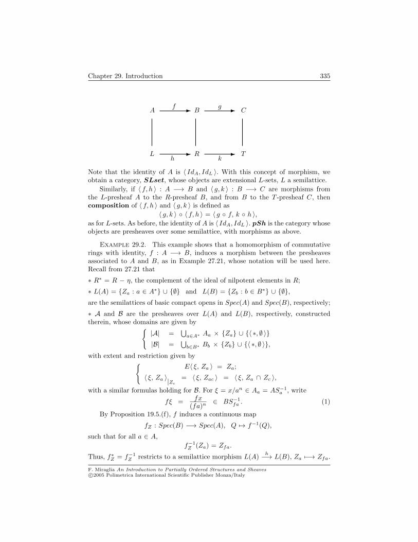
Chapter 29. Introduction 335
L
A - Bf
Rh- - T
- Cg
k
Note that the identity of A is 〈 IdA, IdL 〉. With this concept of morphism, weobtain a category, SLset, whose objects are extensional L-sets, L a semilattice.
Similarly, if 〈 f, h 〉 : A −→ B and 〈 g, k 〉 : B −→ C are morphisms fromthe L-presheaf A to the R-presheaf B, and from B to the T -presheaf C, thencomposition of 〈 f, h 〉 and 〈 g, k 〉 is defined as
〈 g, k 〉 〈 f, h 〉 = 〈 g f, k h 〉,as for L-sets. As before, the identity of A is 〈 IdA, IdL 〉. pSh is the category whoseobjects are presheaves over some semilattice, with morphisms as above.
Example 29.2. This example shows that a homomorphism of commutativerings with identity, f : A −→ B, induces a morphism between the presheavesassociated to A and B, as in Example 27.21, whose notation will be used here.Recall from 27.21 that
∗ R∗ = R − η, the complement of the ideal of nilpotent elements in R;
∗ L(A) = Za : a ∈ A∗ ∪ ∅ and L(B) = Zb : b ∈ B∗ ∪ ∅,are the semilattices of basic compact opens in Spec(A) and Spec(B), respectively;
∗ A and B are the presheaves over L(A) and L(B), respectively, constructedtherein, whose domains are given by
|A| =⋃a∈A∗ Aa × Za ∪ 〈 ∗, ∅ 〉
|B| =⋃b∈B∗ Bb × Zb ∪ 〈 ∗, ∅ 〉,
with extent and restriction given byE〈 ξ, Za 〉 = Za;
〈 ξ, Za 〉|Zc= 〈 ξ, Zac 〉 = 〈 ξ, Za ∩ Zc 〉,
with a similar formulas holding for B. For ξ = x/an ∈ Aa = AS−1a , write
fξ =fx
(fa)n∈ BS−1
fa . (1)
By Proposition 19.5.(f), f induces a continuous map
fZ : Spec(B) −→ Spec(A), Q 7→ f−1(Q),
such that for all a ∈ A,
f−1Z (Za) = Zfa.
Thus, f∗Z = f−1Z restricts to a semilattice morphism L(A)
h−→ L(B), Za 7−→ Zfa.
F. Miraglia An Introduction to Partially Ordered Structures and Sheavesc©2005 Polimetrica International Scientific Publisher Monza/Italy

Chapter 29. Introduction 336
Define γ : |A| −→ |B| by
γ(〈 ξ, Za 〉) = 〈 fξ, Zfa 〉.By (1) above the value of γ is indeed in |B|. Since h(Za) = Zfa, γ satisfies [pmor 1]in 29.1.(b). If 〈 ξ, Za 〉 ∈ |A| and Zc ∈ L(A), we have
γ(〈 ξ, Za 〉|Zc) = γ(〈 ξ, Zac 〉) = 〈 fξ, Zf(ac) 〉 = 〈 fξ, Zfafc 〉
= γ(〈 ξ, Za 〉)|Zfc = γ(〈 ξ, Za 〉)|h(Zc),
verifying [pmor 2]. Hence, 〈 γ, h 〉 is a morphism from A to B, as desired. The readerwill have noticed that γ is simply the “gluing” of the natural ring homomorphismsfrom AS−1
a to BS−1fa of Lemma 9.42.(b), a ∈ A. 2
The classical concept of morphism of presheaves over distinct topological spacesfollows. It has already appeared − without a formal definition −, in Propositions20.9 and 24.64.
Definition 29.3. Let A, B be presheaves over the topological spaces X andY , respectively. A morphism from A to B consists of a pair 〈 η, f 〉 such that
∗ f : Y −→ X is a continuous map;
∗ η = ηU : U ∈ Ω(X), where ηU : A(U) −→ B(f−1(U)) is a map such that ifV ≤ U in Ω(X), the following diagram is commutative :
A(V )
A(U)
?
- B(f−1(U))
·|V
ηU
B(f−1(V ))
·|f−1(V )
ηV
?-
Write 〈 η, f 〉 : A −→ B for a morphism from A to B. If we have morphisms,
A〈η,f〉−→ B
〈µ,g〉−→ C,
their composition is 〈µ η, f g 〉. The identity of A is 〈 IdA, IdX 〉1. Write pShtfor the category of presheaves over some topological space.
The connection between the classical notion of morphism and that in 29.1 isdescribed in
Lemma 29.4. Let A, B be extensional presheaves over the spaces X, Y , re-spectively. The following conditions are equivalent :
(1) 〈 η, f 〉 is a morphism from A to B;
(2) 〈 η, f∗ 〉 is a morphism from the Ω(X)-presheaf A to the Ω(Y )-presheaf B,according to 29.1.(b);
(3) 〈 η, f∗ 〉 is a morphism from the Ω(X)-set A to the Ω(Y )-set B, accordingto 29.1.(a).
1Pointing in the appropriate directions.
F. Miraglia An Introduction to Partially Ordered Structures and Sheavesc©2005 Polimetrica International Scientific Publisher Monza/Italy

Chapter 29. Introduction 337
Proof. It is clear that (1) and (2) are equivalent; for (2)⇔ (3), the argumentis the same as that used to show the equivalence in item (f) of Proposition 26.8.
Definition 29.5. Let A be a L-set and B a R-set. A morphism in SLset,〈 f, h 〉 : A −→ B, is a retract if it has a right inverse, that is, there is a morphism〈 g, k 〉 : B −→ A in SLset such that
〈 f, h 〉 〈 g, k 〉 = 〈 IdB , IdR 〉.Analogously, one defines a retract in pSh.
Lemma 29.6. Suppose L, R are frames, h : L −→ R is a frame-morphism.If 〈 f, h 〉 : A −→ B is a retract in SLset and A is a sheaf over L, then B is asheaf over R.
Proof. Let 〈 g, k 〉 : B −→ A be a morphism such that 〈 f g, h k 〉 =〈 IdB , IdR 〉. For p ∈ R, suppose S ⊆ |B| is compatible over p. By 29.8,gS = gs : s ∈ S is compatible over g(p) (in |A|), and for all s, s′ ∈ S,
Egs = k(Es) and k(p ∧ Es ∧ Es′) = k(p) ∧ [[gs = gs′]].
Let t be a gluing of gS over k(p) in |A|. Then,k(p) ∧ Et =
∨s∈S k(p) ∧ k(Es);
∀ s ∈ S, k(p) ∧ [[t = gs]] = k(p) ∧ Egs = k(p ∧ Es).Consequently, since h preserves joins, we obtain
p ∧ Eft = h(k(p) ∧ Et) = h(k(p) ∧
∨s∈S k(Es)
)= h(k(p)) ∧
∨s∈S h(k(Es)) = p ∧
∨s∈S Es,
as well as, for each s ∈ S,
p ∧ [[ft = s]] = h(k(p)) ∧ [[ft = fgs]] ≥ h(k(p)) ∧ h([[t = gs]])
= h(k(p) ∧ [[t = gs]]) = h(k(p ∧ Es)) = p ∧ Es,and so ft is the gluing of S over p in |B|.
Corollary 29.7. If f : A −→ B is a retract of presheaves over a frame,then Imf = B is a sheaf, whenever the same is true of A.
To understand the categorical content of direct and inverse image, fix a semi-lattice morphism h : L −→ R. If A is a L-set, consider the category of A-algebrasover h 2, whose objects are diagrams
I = (A〈f,h〉−→ B),
with B a R-set. If J = (A〈g,h〉−→ C) is an object of this type, a morphism,
α : I −→ J , consists of a morphism of R-sets, α : B −→ C, such that the di-agram below-left is commutative :
2Analogous to 16.6; sometimes called a comma category.
F. Miraglia An Introduction to Partially Ordered Structures and Sheavesc©2005 Polimetrica International Scientific Publisher Monza/Italy
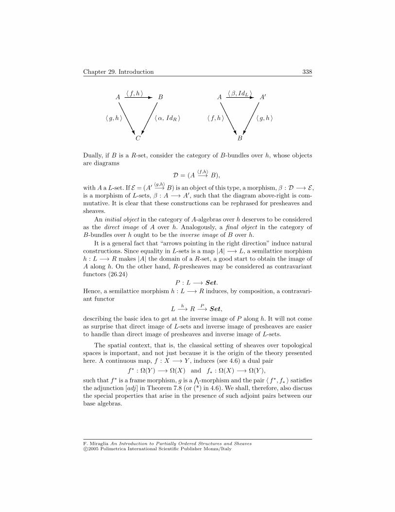
Chapter 29. Introduction 338
A - B
〈 g, h 〉 〈α, IdR 〉
C
〈 f, h 〉
AAAAAU
A - A′
〈 f, h 〉 〈 g, h 〉
B
〈β, IdL 〉
AAAAAU
Dually, if B is a R-set, consider the category of B-bundles over h, whose objectsare diagrams
D = (A〈f,h〉−→ B),
withA a L-set. If E = (A′〈g,h〉−→ B) is an object of this type, a morphism, β : D −→ E ,
is a morphism of L-sets, β : A −→ A′, such that the diagram above-right is com-mutative. It is clear that these constructions can be rephrased for presheaves andsheaves.
An initial object in the category of A-algebras over h deserves to be consideredas the direct image of A over h. Analogously, a final object in the category ofB-bundles over h ought to be the inverse image of B over h.
It is a general fact that “arrows pointing in the right direction” induce naturalconstructions. Since equality in L-sets is a map |A| −→ L, a semilattice morphismh : L −→ R makes |A| the domain of a R-set, a good start to obtain the image ofA along h. On the other hand, R-presheaves may be considered as contravariantfunctors (26.24)
P : L −→ Set.
Hence, a semilattice morphism h : L −→ R induces, by composition, a contravari-ant functor
Lh−→ R
P−→ Set,
describing the basic idea to get at the inverse image of P along h. It will not comeas surprise that direct image of L-sets and inverse image of presheaves are easierto handle than direct image of presheaves and inverse image of L-sets.
The spatial context, that is, the classical setting of sheaves over topologicalspaces is important, and not just because it is the origin of the theory presentedhere. A continuous map, f : X −→ Y , induces (see 4.6) a dual pair
f∗ : Ω(Y ) −→ Ω(X) and f∗ : Ω(X) −→ Ω(Y ),
such that f∗ is a frame morphism, g is a∧
-morphism and the pair 〈 f∗, f∗ 〉 satisfiesthe adjunction [adj] in Theorem 7.8 (or (*) in 4.6). We shall, therefore, also discussthe special properties that arise in the presence of such adjoint pairs between ourbase algebras.
F. Miraglia An Introduction to Partially Ordered Structures and Sheavesc©2005 Polimetrica International Scientific Publisher Monza/Italy
Chapter 29. Introduction 339
Exercises
29.8. a) If 〈 f, h 〉 : A −→ B is a morphisms in LSset or pSh, and S ⊆ |A|is compatible over p, then
fS = fs : s ∈ S ⊆ |B|is compatible over h(p).
b) If Lh−→ R is a [∧,
∨]-morphism, a morphism 〈 f, h 〉 : A −→ B in SLset or
pSh preserves gluings of compatible families. 2
F. Miraglia An Introduction to Partially Ordered Structures and Sheavesc©2005 Polimetrica International Scientific Publisher Monza/Italy
CHAPTER 30
Image of a L-set
Let A be L-set and Lh−→ R be a semilattice morphism. We can transport the
L-equality in |A| along h, to get an R-equality on |A|, given by
[[x = y]]AR = h([[x = y]]A).
Write AR for the R-set so defined. In general, AR is not extensional, even if A isextensional. We now describe a different procedure, which furnishes an extensionalchange of base.
30.1. Let h : L −→ R be a semilattice morphism and let A be a L-set. Definea binary relation θA on |A|, by
x θA y iff h(EAx) = h([[x = y]]A) = h(EAy). (I)
It is readily verified that θA is an equivalence relation on |A|; let
∗ |εhA| be the set of θA-equivalence classes on |A|;
∗ εAh : |A| −→ |εhA| be the canonical quotient map. Whenever A is clear fromcontext, we omit the superscript A from the notation. 2
Remark 30.2. If h is injective and A is extensional, θA is the identity. Hence,in this case, εhA = AR. Furthermore, for all p ∈ L, εh|A(p)
is a bijection between
A(p) and εhA(h(p)). 2
Proposition 30.3. Let h : L −→ R be a semilattice morphism and let A bea L-set.
a) For x, y ∈ |A|, the map
〈 εhx, εhy 〉 7−→ h([[x = y]]A)
defines an extensional equality on |εhA|, with which it is a R-set. Furthermore,〈 εh, h 〉 : A −→ εhA is a morphism in SLset, such that for all x, y ∈ |A|
E(εhx) = h(Ex) and [[εhx = εhy]] = h([[x = y]]).
b) If B an extensional R-set and 〈 f, h 〉 a morphism from A to B, then there
is a unique morphism f : Ah −→ B in Rset such that the following diagramcommutes :
340
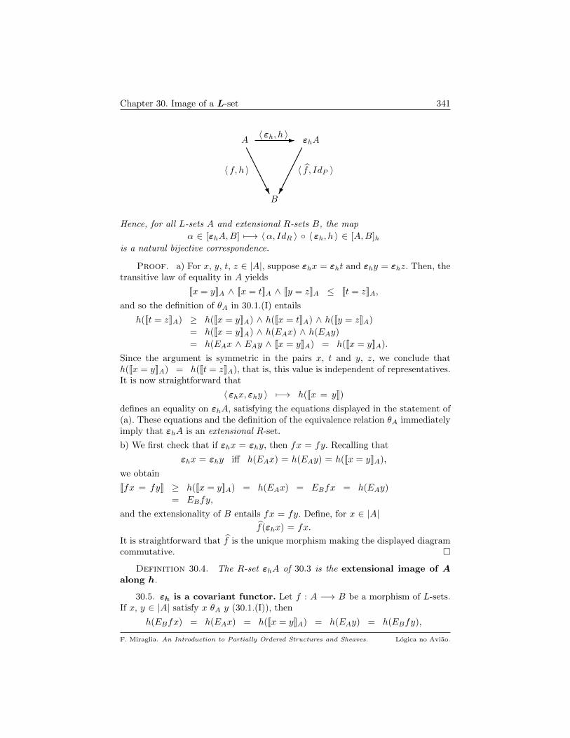
Chapter 30. Image of a L-set 341
A - εhA
〈 f, h 〉 〈 f , IdP 〉
B
〈 εh, h 〉
AAAAAU
Hence, for all L-sets A and extensional R-sets B, the map
α ∈ [εhA,B] 7−→ 〈α, IdR 〉 〈 εh, h 〉 ∈ [A,B]his a natural bijective correspondence.
Proof. a) For x, y, t, z ∈ |A|, suppose εhx = εht and εhy = εhz. Then, thetransitive law of equality in A yields
[[x = y]]A ∧ [[x = t]]A ∧ [[y = z]]A ≤ [[t = z]]A,
and so the definition of θA in 30.1.(I) entails
h([[t = z]]A) ≥ h([[x = y]]A) ∧ h([[x = t]]A) ∧ h([[y = z]]A)
= h([[x = y]]A) ∧ h(EAx) ∧ h(EAy)
= h(EAx ∧ EAy ∧ [[x = y]]A) = h([[x = y]]A).
Since the argument is symmetric in the pairs x, t and y, z, we conclude thath([[x = y]]A) = h([[t = z]]A), that is, this value is independent of representatives.It is now straightforward that
〈 εhx, εhy 〉 7−→ h([[x = y]])
defines an equality on εhA, satisfying the equations displayed in the statement of(a). These equations and the definition of the equivalence relation θA immediatelyimply that εhA is an extensional R-set.
b) We first check that if εhx = εhy, then fx = fy. Recalling that
εhx = εhy iff h(EAx) = h(EAy) = h([[x = y]]A),
we obtain
[[fx = fy]] ≥ h([[x = y]]A) = h(EAx) = EBfx = h(EAy)
= EBfy,
and the extensionality of B entails fx = fy. Define, for x ∈ |A|f(εhx) = fx.
It is straightforward that f is the unique morphism making the displayed diagramcommutative.
Definition 30.4. The R-set εhA of 30.3 is the extensional image of Aalong h.
30.5. εh is a covariant functor. Let f : A −→ B be a morphism of L-sets.If x, y ∈ |A| satisfy x θA y (30.1.(I)), then
h(EBfx) = h(EAx) = h([[x = y]]A) = h(EAy) = h(EBfy),
F. Miraglia. An Introduction to Partially Ordered Structures and Sheaves. Logica no Aviao.
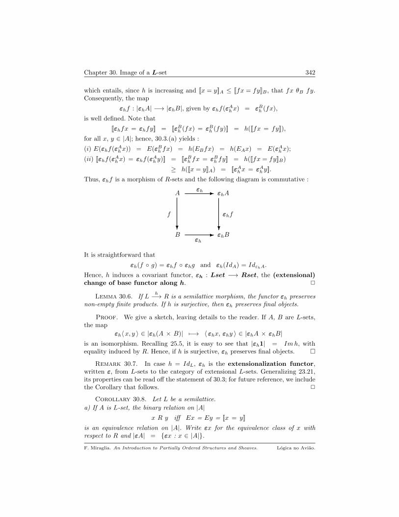
Chapter 30. Image of a L-set 342
which entails, since h is increasing and [[x = y]]A ≤ [[fx = fy]]B , that fx θB fy.Consequently, the map
εhf : |εhA| −→ |εhB|, given by εhf(εAh x) = εBh (fx),
is well defined. Note that
[[εhfx = εhfy]] = [[εBh (fx) = εBh (fy)]] = h([[fx = fy]]),
for all x, y ∈ |A|; hence, 30.3.(a) yields :
(i) E(εhf(εAh x)) = E(εBh fx) = h(EBfx) = h(EAx) = E(εAh x);
(ii) [[εhf(εAh x) = εhf(εAh y)]] = [[εBh fx = εBh fy]] = h([[fx = fy]]B)
≥ h([[x = y]]A) = [[εAh x = εAh y]].
Thus, εhf is a morphism of R-sets and the following diagram is commutative :
B
A
?
- εhA
f
εh
εhB
εhf
εh
?-
It is straightforward that
εh(f g) = εhf εhg and εh(IdA) = IdεhA.
Hence, h induces a covariant functor, εh : Lset −→ Rset, the (extensional)change of base functor along h. 2
Lemma 30.6. If Lh−→ R is a semilattice morphism, the functor εh preserves
non-empty finite products. If h is surjective, then εh preserves final objects.
Proof. We give a sketch, leaving details to the reader. If A, B are L-sets,the map
εh〈x, y 〉 ∈ |εh(A × B)| 7−→ 〈 εhx, εhy 〉 ∈ |εhA × εhB|is an isomorphism. Recalling 25.5, it is easy to see that |εh1| = Imh, withequality induced by R. Hence, if h is surjective, εh preserves final objects.
Remark 30.7. In case h = IdL, εh is the extensionalization functor,written ε, from L-sets to the category of extensional L-sets. Generalizing 23.21,its properties can be read off the statement of 30.3; for future reference, we includethe Corollary that follows. 2
Corollary 30.8. Let L be a semilattice.
a) If A is L-set, the binary relation on |A|x R y iff Ex = Ey = [[x = y]]
is an equivalence relation on |A|. Write εx for the equivalence class of x withrespect to R and |εA| = εx : x ∈ |A|.
F. Miraglia. An Introduction to Partially Ordered Structures and Sheaves. Logica no Aviao.

Chapter 30. Image of a L-set 343
b) For x, y ∈ |A|, set
[[εx = εy]] = [[x = y]].
This defines an extensional equality on |εA|, such that Eεx = Ex, for all x ∈ |A|.c) The map ε : A −→ εA, x 7→ εx is a L-set morphism, with the following universalproperty :
If B is an extensional L-set and f : A −→ B is a morphism of L-sets, there
is a unique morphism of L-sets, f : εA −→ B, making the diagram below-leftcommutative :
A - εA
f f
B
ε
AAAAAU
B
A
?
- εA
f
ε
εB
εf
ε
?-
d) If Af−→ B is a morphism of L-sets, the map
εf : |εA| −→ |εB|, defined by εx 7→ εfx,
is the unique morphism of L-sets making the diagram above-right commutative. 2
The composition of εh with the completion functor in 27.9 yields
Corollary 30.9. Let Lh−→ Ω be a semilattice morphism, with Ω a frame.
If A is a L-set, then there is a sheaf chA over Ω and a morphism
〈 ch, h 〉 : A −→ chA,
verifying the following conditions :
(1) For all a, b ∈ |A|, [[cha = chb]] = h([[a = b]]);
(2) For all s ∈ |cA|, Es =∨a∈|A| [[cha = s]];
(3) If C is a sheaf over Ω and 〈 g, h 〉 : A −→ C is a morphism, there is aunique morphism g : chA −→ C in Sh(Ω) such that the following diagram iscommutative :
A - chA
〈 g, h 〉 〈 g, IdΩ 〉
C
〈 ch, h 〉
AAAAAU
2
The sheaf chA is the completion of A along h. When h = IdΩ, we get backthe completion cA of Theorem 27.9; furthermore,
F. Miraglia. An Introduction to Partially Ordered Structures and Sheaves. Logica no Aviao.

Chapter 30. Image of a L-set 344
〈 ch, h 〉 = 〈 c, IdΩ 〉 〈 εh, h 〉,with c the completion map of 27.9. Since every [∧,
∨]-semilattice can be regularly
embedded in a frame (25.29), we get
Corollary 30.10. If L is a [∧,∨
]-semilattice and A is a L-set, there is aregular embedding, h : L −→ Ω, a sheaf chA over Ω together with a morphism,ch : A −→ chA, such that, if L is identified with h(L), conditions (1), (2) and (3)in 27.9 are verified 1.
In particular, if H is a HA, then any H-set gives rise to a sheaf over H∗, theframe completion of H (14.4). Exercise 30.14 shows that this completion deservesto be considered the completion of the H-set under consideration.
The functor ch may also be used to define image in the category of sheaves :
Definition 30.11. If L is a frame, h : L −→ Ω is a semilattice morphismand A is a sheaf over L, the sheaf chA is the image of A along h in the categoryof Sh(Ω).
We now show that image along a semilattice morphism preserves composition.This result has many applications, considerably simplifying the computation ofthe transfer of objects along maps between the base algebras.
Proposition 30.12. Let Lf−→ R
g−→ T be semilattice morphisms. Then,
a) ε(g f) = εg εf 2.
b) If L, R, T are frames, then c(g f) = cg cf .
c) If T = L and g f = IdL, εg εg and cg cf are the identity functors in theextensional subcategory of Lset and in Sh(L), respectively.
Proof. a) We prove (a), leaving (b) as an exercise. Let A be a L-set and〈α, gf 〉 : A −→ B be a morphism in pSh into the extensional T -set B.
Fact. The map εfa ∈ |εfA|β7−→ αa ∈ |B| is the carrier of the unique morphism,
〈β, g 〉 : εfA −→ B, making the following triangle commutative :
A - εfA
〈α, gf 〉 〈β, g 〉
B
〈 εf , f 〉
AAAAAU
Proof. If a, b ∈ |A| are such that εfa = εfb, then
f(Ea) = f(Eb) = f([[a = b]])
1With ch in place of c, of course.2I.e., these functors are naturally isomorphic; the same comment applies to (b).
F. Miraglia. An Introduction to Partially Ordered Structures and Sheaves. Logica no Aviao.
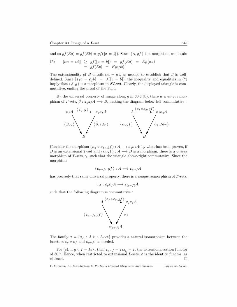
Chapter 30. Image of a L-set 345
and so gf(Ea) = gf(Eb) = gf([[a = b]]). Since 〈α, gf 〉 is a morphism, we obtain
(*) [[αa = αb]] ≥ gf([[a = b]]) = gf(Ea) = EB(αa)
= gf(Eb) = EB(αb).
The extensionality of B entails αa = αb, as needed to establish that β is well-defined. Since [[εfa = εfb]] = f([[a = b]]), the inequality and equalities in (*)imply that 〈β, g 〉 is a morphism in SLset. Clearly, the displayed triangle is com-mutative, ending the proof of the Fact.
By the universal property of image along g in 30.3.(b), there is a unique mor-
phism of T -sets, β : εgεfA −→ B, making the diagram below-left commutative :
εfA - εgεfA
〈β, g 〉 〈 β, IdT 〉
B
〈 εg, g 〉
AAAAAU
A - εfεgA
〈α, gf 〉 〈 γ, IdT 〉
B
〈 εf εg, gf 〉
AAAAAU
Consider the morphism 〈 εg εf , gf 〉 : A −→ εgεfA; by what has been proven, ifB is an extensional T -set and 〈α, gf 〉 : A −→ B is a morphism, there is a uniquemorphism of T -sets, γ, such that the triangle above-right commutative. Since themorphism
〈 εg f , gf 〉 : A −→ εg fA
has precisely that same universal property, there is a unique isomorphism of T -sets,
σA : εgεfA −→ ε(g f)A,
such that the following diagram is commutative :
A - εgεfA
〈 εg f , gf 〉 σA
ε(g f)A
〈 εf εg, gf 〉
AAAAAU
The family σ = σA : A is a L-set provides a natural isomorphism between thefunctors εg εf and εg f , as needed.
For (c), if g f = IdL, then εg f = εIdL = ε, the extensionalization functorof 30.7. Hence, when restricted to extensional L-sets, ε is the identity functor, asclaimed.
F. Miraglia. An Introduction to Partially Ordered Structures and Sheaves. Logica no Aviao.
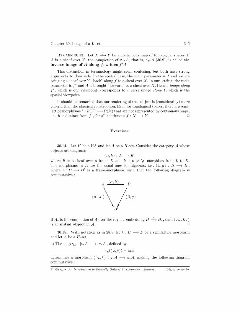
Chapter 30. Image of a L-set 346
Remark 30.13. Let Xf−→ Y be a continuous map of topological spaces. If
A is a sheaf over Y , the completion of εf∗A, that is, cf∗A (30.9), is called theinverse image of A along f , written f∗A.
This distinction in terminology might seem confusing, but both have strongarguments to their side. In the spatial case, the main parameter is f and we arebringing a sheaf over Y “back” along f to a sheaf over X. In our setting, the mainparameter is f∗ and A is brought “forward” to a sheaf over X. Hence, image alongf∗, which is our viewpoint, corresponds to inverse image along f , which is thespatial viewpoint.
It should be remarked that our rendering of the subject is (considerably) moregeneral than the classical construction. Even for topological spaces, there are semi-lattice morphisms h : Ω(Y ) −→ Ω(X) that are not represented by continuous maps,i.e., h is distinct from f∗, for all continuous f : X −→ Y . 2
Exercises
30.14. Let H be a HA and let A be a H-set. Consider the category A whoseobjects are diagrams
〈α, k 〉 : A −→ B,
where B is a sheaf over a frame D and k is a [∧,∨
]-morphism from L to D.The morphisms in A are the usual ones for algebras, i.e., 〈β, g 〉 : B −→ B′,where g : D −→ D′ is a frame-morphism, such that the following diagram iscommutative :
A - B
〈α′, k′ 〉 〈β, g 〉
B′
〈α, k 〉
AAAAAU
If A∗ is the completion of A over the regular embedding H∗−→ H∗, then 〈A∗, H∗ 〉
is an initial object in A. 2
30.15. With notation as in 28.5, let k : H −→ L be a semilattice morphismand let A be a H-set.
a) The map γk : |skA| −→ |εkA|, defined by
γk(〈x, p 〉) = εkx
determines a morphism 〈 γk, k 〉 : skA −→ εkA, making the following diagramcommutative :
F. Miraglia. An Introduction to Partially Ordered Structures and Sheaves. Logica no Aviao.
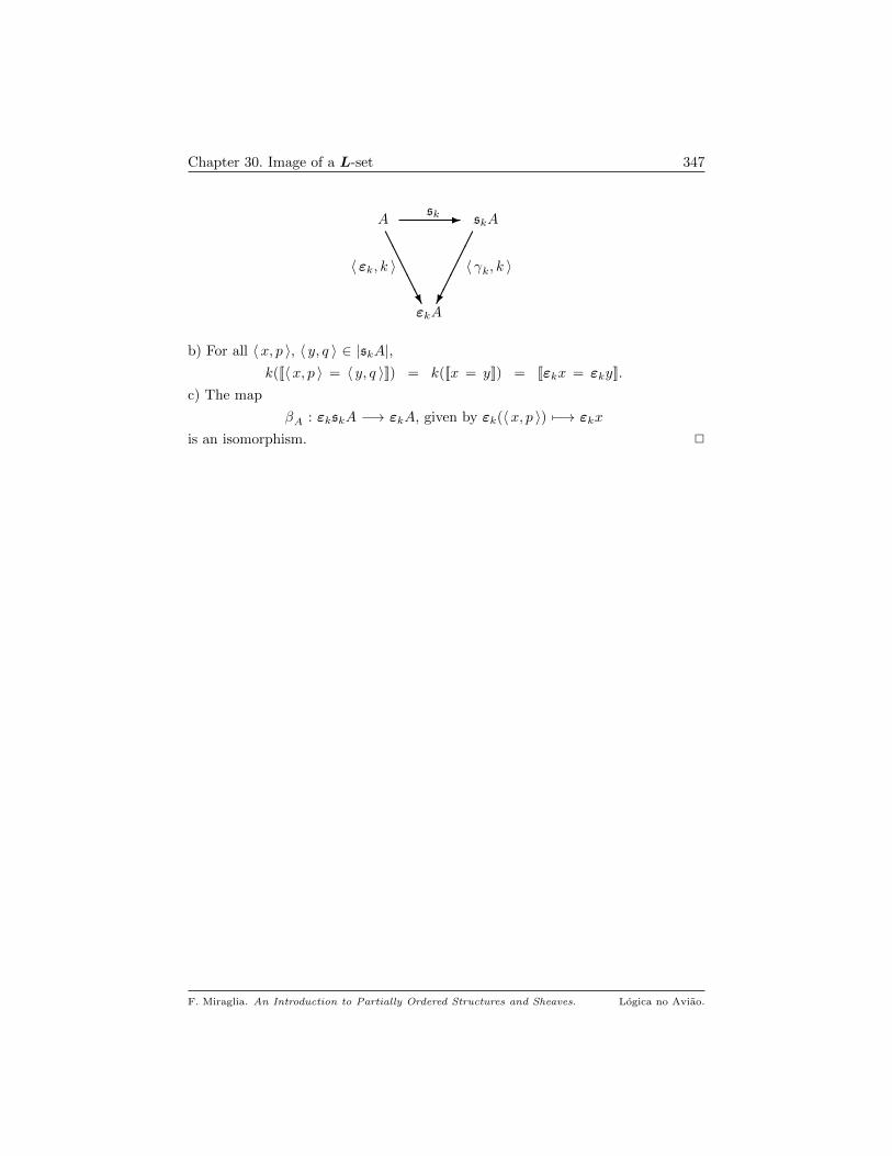
Chapter 30. Image of a L-set 347
A - skA
〈 εk, k 〉 〈 γk, k 〉
εkA
sk
AAAAAU
b) For all 〈x, p 〉, 〈 y, q 〉 ∈ |skA|,k([[〈x, p 〉 = 〈 y, q 〉]]) = k([[x = y]]) = [[εkx = εky]].
c) The map
βA : εkskA −→ εkA, given by εk(〈x, p 〉) 7−→ εkx
is an isomorphism. 2
F. Miraglia. An Introduction to Partially Ordered Structures and Sheaves. Logica no Aviao.

CHAPTER 31
Base Extension
By 26.5 and 26.25, whenever L ⊆ R, a R-presheaf may be restricted to L,originating a functor, r : pSh(R) −→ pSh(L). This Chapter is devoted to theinverse operation. Section 16.4 and Chapter 17 are references for the colimitsemployed below.
31.1. We return to the context of Chapter 23. Let L be a semilattice, consi-dered a category as in Example 16.4. Let C be a category that has colimits for alldiagrams over up-directed posets and fix a covariant functor 1
A : Lop −→ C.We write the values of A at p ∈ L as A(p) and if p ≤ q ∈ L,
x ∈ A(q) 7−→ x|p ∈ A(p)
for the morphism corresponding to the pair p ≤ q. For p ≤ q ≤ r and x ∈ A(r),the functoriality of A entails
x|r = x and x|p = (x|q)|p.These equalities imply that a down-directed subset F of L gives rise to an inductivesystem in C, A(F ), given by :
A(F ) = 〈A(q); ∗|p : p ≤ q in F 〉.
Note that A(F ) is an inductive system over the up-directed subset F op of L. Write
AF = lim→p∈FA(p) = lim→ A(F )
for the colimit of A(F ). Recall that AF comes equipped with C-morphisms
fFp : A(p) −→ AF , p ∈ F ,
making the following diagram commutative, for p ≤ q in F :
A(q) - A(p)
fFq fFp
AF
∗|p
AAAAAU
1That is, a L-presheaf with values in C.
348

Chapter 31. Base Extension 349
It is clear that if F has a least element p, then AF = A(p) and that the morphismfFq is the restriction from A(q) to A(p).
If G is another down-directed subset of L, with F ⊆ G, then for all p ∈ F ,there is a map fGp : A(p) −→ AG, making the diagram below-left commutative,where p ≤ q in F :
A(q) - A(p)
fGq fGp
AG
∗|p
AAAAAU
A(p) - AF
fGp αFG
AG
fFp
AAAAAU
Since AF = lim→ A(F ), there is a unique C-morphism,
αFG : AF −→ AG,
making the diagram above right commutative, for all p ∈ F . We call αFG therestriction from AF to AG.
A final comment : if F is empty, AF is also empty. Thus, if G is a down-directedsubset of L, the restriction map αFG is the empty map from AF to AG. 2
By Exercise 26.24, the category of L-presheaves is isomorphic to that of covari-ant functors from Lop to Set, with natural transformations as morphisms. We maytherefore apply the general scheme described in 31.1 to the extension problem.
31.2. Let A be a L-presheaf and suppose that R is a semilattice, containingL as a subsemilattice. For each u ∈ R, set
G(u) = p ∈ L : u ≤ p.Clearly, G(u) is down-directed and, in fact, closed under meets. Let eA(u) be thecolimit of the system associated to G(u) and A, which comes equipped with mapsfpu : A(p) −→ eA(u), making the diagram below-left commutative :
A(q) - A(p)
fqu fpu
eA(u)
∗|p
AAAAAU
A(p) - eA(u)
fpv αuv
eA(v)
fpu
AAAAAU
Note that if v ≤ u in R, then G(u) ⊆ G(v), and 31.1 guarantees that thereis a unique map, αuv : eA(u) −→ eA(v), such that the diagram above-right iscommutative, for all p ∈ G(u). It is straightforward to verify that if r ≤ v ≤ u inR, then
(*) αuu = IdeA(u) and αur = αuv αvr.
F. Miraglia. An Introduction to Partially Ordered Structures and Sheaves. Logica no Aviao.

Chapter 31. Base Extension 350
Moreover, if p ∈ L, then p = min G(p) and we have :
(**)
(i) eA(p) = A(p); (ii) ∀ q ∈ G(p), αqp = ∗|p;
(iii) If p ∈ G(r), then αpr = fpr.
We now define a R-presheaf, eA, as follows :
(eA)
a) |eA| =
∐u∈R eA(u);
b) EeA(s) = u iff s ∈ eA(u);
c) For s ∈ |eA| and v ∈ R, s|v = αEs,Es∧v(s).
2
Proposition 31.3. Notation as in 31.2, let A be a L-presheaf and R a semi-lattice containing L as a subsemilattice. Then,
a) eA is a R-presheaf.
b) The map e : |A| −→ |eA| defined by
a ∈ |A| 7−→ ea ∈ eA(Ea) = A(Ea)
is an injection, such that for all 〈x, p 〉 ∈ |A| × L
Eex = Ex and e(x|p) = (ex)|p.
Moreover, for all s ∈ |eA|, there is p ∈ G(Es) and x ∈ A(p) such that s = x|Es2.
c) If L is complete and A is extensional, then eA is extensional.
d) If B is a R-presheaf and |A| g−→ |B| is a map such that for all 〈x, p 〉 ∈ |A| × L
Egx = Ex and g(x|p) = (gx)|p,
then there is a unique morphism of R-presheaves, f : eA −→ B, such that thediagram below-left is commutative :
A - eA
g f
B
e
AAAAAU
A - (eA)|L
e reA
eA
ρA
AAAAAU
e) There is a natural isomorphism, ρA : A −→ (eA)|L, making the diagram
above-right is commutative 3.
Proof. a) That eA is a R-presheaf follows easily from the equalities in (*)of 31.2. For instance, if x ∈ |eA| and u, v ∈ R, then
(x|u)|v = x|u∧vis an immediate consequence of the second equation in 31.2.(*).
2Thus, the image of e is restriction dense in eA; see 26.28.(d).3Notation as in 26.5 and 26.25.
F. Miraglia. An Introduction to Partially Ordered Structures and Sheaves. Logica no Aviao.

Chapter 31. Base Extension 351
b) Clearly, e has the stated properties. Fix s ∈ eA(u); since eA(u) = lim→p∈G(u)A(p),
there is p ∈ G(u) and x ∈ A(p), such that fpu(x) = s. But (eA) in 31.2 then entailsx|u = s in eA 4.
c) Assume that A is extensional and L is complete. Let s, t ∈ eA(u) be sectionssuch that there is α ⊆ R satisfying∨
α = u and s|v = t|v, for all v ∈ α.
By item (b), there are p, q ∈ G(u), x ∈ A(p) and y ∈ A(q), such that x|u = s and
y|u = t. Since G(u) is down-directed, we may as well assume that p = q (otherwise,
substitute both for p ∧ q). For v ∈ α, we have
x|v = x|u∧v = (x|u)|v = s|v = t|v = y|v.Since eA(v) = lim→r∈G(v)
A(r), there is qv ∈ G(v) such that x|qv = y|qv . Because
v ≤ u ≤ p, we may assume that qv ≤ p (otherwise, replace qv by its meet with p).It is clear that
u ≤ q =def
∨v∈α qv ∈ L.
Consider x′ = x|q, y′ = y|q ∈ A(q); since s = x|u and t = y|u, we also have s = x′|u
and t = y′|u. Now observe that for all v ∈ α,
x′|qv = (x|q)|qv = x|q∧qv = x|qv = y|qv = y′|qv ,
and the extensionality of A entails x′ = y′. Thus, s = x′|u = y′|u = t, establishing
the extensionality of eA.
d) For u ∈ R and p ∈ G(u), since Egx = Ex, define
gpu : A(p) −→ B(u), by x ∈ A(p) 7−→ (gx)|u ∈ B(u).
Since g commutes with the restrictions by elements in L, the diagram below leftis commutative, where q ≤ p, both in G(u) :
A(p) - A(q)
gpu gqu
B(u)
∗|p
AAAAAU
A(p) - eA(u)
gpu fu
B(u)
fpu
AAAAAU
Since eA(u) = lim→p∈G(u)A(p), there is a unique fu : eA(u) −→ B(u), such that the
diagram above-right is commutative, for all p inG(u). The family f = fu : u ∈ Rdetermines the required morphism of R-presheaves. Details are left to the reader.
4We are, of course, identifying A with its image by the injection e.
F. Miraglia. An Introduction to Partially Ordered Structures and Sheaves. Logica no Aviao.
Chapter 31. Base Extension 352
d) By 23.26.(a) (and (b) in the present result), there is a unique morphism ofL-presheaves, ρA : A −→ (eA)|L, such that the diagram in the statement is com-
mutative. Since for all p ∈ L we have
(eA)|L(p) = eA(p) = A(p),
it is clear that ρA is a bijection when restricted to A(p). Hence, ρA is an isomor-phism between A and (eA)|L.
Definition 31.4. The R-presheaf eA of 31.3 is the extension of A to R.
Example 31.5. Let g : C −→ D be a non-injective map of sets. Fix a, b inC, such that g(a) = g(b). Let
L = [0, 1/2) ∪ (1/2, 1] ⊆ [0, 1] = R,
the unit real interval. Both L and R have their natural orders. Note that R is aframe and L is a [∧,
∨]-sublattice of R. Define a L-presheaf A as follows :
(i) |A| =⋃p∈[0,1/2) D × p ∪
⋃p∈(1/2,1] C × p;
(ii) E〈x, p 〉 = p;
(iii) 〈x, p 〉|q =
〈 g(x), p 〉 if p ∈ [0, 1/2) and q ∈ (1/2, 1]
〈x, p ∧ q 〉 otherwise.
A is extensional for the simple reason that no element of (1/2, 1] is the join ofelements in [0, 1/2). If p ≤ q in L, the restriction maps of A are given by
ρqp =
IdC if p, q ∈ (1/2, 1]
IdD if p, q ∈ [0, 1/2)
g if p ∈ [0, 1/2) and q ∈ (1/2, 1].
Consequently, eA(1/2) = lim→p>1/2A(p) = C; further, for p < 1/2, the restric-
tion map from eA(1/2) to A(p) is g. Hence, for all p ∈ [0, 1/2),
a|p = b|p,
although a 6= b in eA(1/2). This shows that the hypothesis of completeness of Lin 31.3.(c) is necessary. 2
31.6. Base extension is a covariant functor. Let L ⊆ R be semilatticesand f : A −→ B be a morphism of L-presheaves. It is straightforward that thecomposition
Af−→ B
e−→ eB
verifies the conditions in item (d) of 31.3, and so there is a unique morphism ofR-presheaves, ef : eA −→ eB, making the following diagram commutative :
F. Miraglia. An Introduction to Partially Ordered Structures and Sheaves. Logica no Aviao.

Chapter 31. Base Extension 353
B
A
?
- eA
f
e
eB
ef
e
?-
The proof of 31.3.(d) will yield a concrete description of ef on the elements of |eA|.It is straightforward that
e(IdA) = IdeA and e(g f) = eg ef ,
and so base extension is a covariant functor, e : pSh(L) −→ pSh(R). It has beennoted (26.25) that restriction is also a covariant functor, r : pSh(R) −→ pSh(L).The next result establishes the adjointness of these functors. 2
Proposition 31.7. Let L ⊆ R be semilattices, A be a L-presheaf and B aR-presheaf.
a) There is a natural morphism of R-presheaves, jB : e(B|L) −→ B, making the
following diagram commutative :
B|L - e(B|L)
rB jB
B
e
AAAAAU
b) Extension is left adjoint to restriction, that is, there a bijective correspondence,natural in A and B,
kAB : [eA, B] ≈ [A, B|L],
defined by g 7−→ rg ρA, whose inverse is given by f 7−→ jB ef 5.
Proof. The existence and naturality of jB follows from the universal prop-erty of the morphism e : B|L −→ e(B|L) in 31.3.(d). Item (b) is a straightforward
consequence of the universal properties of extension and restriction (26.25).
Example 31.8. Let M be the sheaf of 23.11, whose base algebra is thecomplete Boolean algebra 2I . Recall that for all u ⊆ I,
M(u) =∏i∈u Mi,
and the restriction maps are the projections that forget the coordinates outsidethe larger domain.
5ρA as in 31.3.(e).
F. Miraglia. An Introduction to Partially Ordered Structures and Sheaves. Logica no Aviao.

Chapter 31. Base Extension 354
Let βI be the Stone-Cech compactification of the discrete set I (21.6). SinceβI is the Stone space of 2I , Stone duality yields a lattice injection
2I −→ Ω(βI),
which identifies each u ⊆ I with the compact clopen Su6. We may, therefore,
consider 2I as a sublattice of Ω(βI). To determine the extension of M to Ω(βI),recall that by 21.2.(b), βI is extremally disconnected, that is, the closure of everyopen set is clopen. Hence, if U ∈ Ω(βI), there is a unique u ∈ 2I , with U = Su.Hence, if v ⊆ I, elementary topology and Stone duality yield
U ⊆ Sv iff Su ⊆ Sv iff u ⊆ v.
Whence, in the notation of 31.2,
G(U) = v ⊆ I : u ⊆ v.and so
eM(U) = lim→v∈G(U)M(v) = M(u) =
∏i∈u Mi,
with restriction maps induced by M. In particular,
eM(βI) =∏i∈I Mi = M(I).
Let T = tk : k ∈ K be a compatible set of sections in |eM|. For each k ∈ K,there is uk ⊆ I and sk ∈ A(uk) such that
Etk = Suk and sk = tk.
Since M is a sheaf, the sk have a unique gluing in M, s, whose extent isv =
⋃k∈K uk. By 19.7.(d).(2), we have
U =def
⋃k∈K Etk ⊆
⋃k∈K Suk ⊆
⋃k∈K Suk = Sv.
Thus, if u ⊆ I is such that U = Su, then Su ⊆ Sv, that is, u ⊆ v. Then, s|u is the
unique gluing of the tk in eM. We have shown that eM is a sheaf over βI. Thus,a sheaf over the discrete space I has given rise, by base extension, to a sheaf overthe non-discrete space βI.
Finally, if s, t ∈ |eM|, then
[[s = t]]eM = Es ∧ Et ∧ S[[s=t]],
where, in the second member of the above equation, the index [[s = t]] is theequality of these terms as elements of |M|. 2
We now describe how restriction (26.5, 26.25) and extension behave on cat-egories of sheaves. By 31.11.(a), extension does not, in general, preserve com-pleteness (but see Exercise 31.14). If L ⊆ R are frames, to construct a functor,ce : Sh(L) −→ Sh(R), we follow the extension functor e of 31.3 by completionover R, obtaining the complete extension functor. Hence, we have functors
r : Sh(R) −→ Sh(L) and ce : Sh(L) −→ Sh(R),
which are still adjoint, as in 31.7.
6Su is the set of ultrafilters F in 2I such that u ∈ F .
F. Miraglia. An Introduction to Partially Ordered Structures and Sheaves. Logica no Aviao.

Chapter 31. Base Extension 355
Corollary 31.9. If L ⊆ R are frames, then complete extension is left ad-joint to restriction, i.e., if A is a L-sheaf and B is a R-sheaf, there is a bijectivecorrespondence, natural in A and B,
[ceA, B] ≈ [A, B|L],
which is induced, as in 31.7, by natural isomorphisms
ρA : A ≈ (ceA)|L and jB : ce(B|L) −→ B.
Proof. Left to the reader.
Exercises
31.10. Prove 31.3.(d) making use of 26.21 and of the fact that A is restrictiondense in eA. 2
31.11. Let L be a semilattice with ⊥ and >. Let 2 = ⊥,> ⊆ L; clearly, 2is a complete subsemilattice of L.
a) Show that if A is a set (i.e., a 2-presheaf, 26.3), then the extension of A to L isthe constant A presheaf on L (26.4).
b) If B is a L-presheaf, then B|L can be naturally identified with the set of global
sections of B over L.
c) “Global section” is a functor from pSh(L) to Set = pSh(2), right adjoint tothe constant presheaf functor. 2
31.12. Let L be a distributive lattice and let A be a L-presheaf. With 31.8 asa model, study the extension of A to the Stone space, S(L), of L. Show that if Uis a compact open in S(L), there is p ∈ L, such that eA(U) = A(p). 2
31.13. If L is a subsemilattice of R and A is a flabby presheaf over R (26.28.(e)),then A|L is a flabby L-presheaf. 2
31.14. If L ⊆ R are frames, then B ∈ Sh(R) ⇒ B|L ∈ Sh(L). 2
F. Miraglia. An Introduction to Partially Ordered Structures and Sheaves. Logica no Aviao.
CHAPTER 32
Image of a Presheaf
As a preliminary to the construction in the title, we discuss the essential imageof a presheaf along h.
32.1. Let Lh−→ R be a semilattice morphism and let A be a L-presheaf. Set
A = 〈 a, q 〉 ∈ |A| × (Imh) : h(Ea) = q.Define a binary relation ϑA on A, as follows :
〈 a, q 〉 ϑA 〈 b, q′ 〉 iff q = q′ and ∃ u ∈ h−1(q) such that a|u = b|u.
ϑA is an equivalence relation on A. For instance, if 〈 a, q 〉 ϑA 〈 b, q′ 〉 and 〈 b, q′ 〉ϑA 〈 c, q′′ 〉, then q = q′ = q′′; moreover, there are u, v ∈ L such that
h(u) = h(v) = q, a|u = b|u and b|v = c|v.
Hence, (u ∧ v) ∈ h−1(q), a|u∧v = c|u∧v, and so 〈 a, q 〉 ϑA 〈 c, q′′ 〉. If r ∈ Imh and
v, w ∈ h−1(r), then for all 〈 a, q 〉 ∈ A,
(ϑ)
(i) 〈 a|v, q ∧ r 〉 ∈ A;
(ii) 〈 a|v, q ∧ r 〉 ϑA 〈 a|w, q ∧ r 〉 ϑA 〈 a|v∧w, q ∧ r 〉.
For (i), we have Ea|v = Ea ∧ v, and therefore h(Ea ∧ v) = q ∧ r. For (ii), let
u = Ea ∧ v ∧ w. Then, h(u) = q ∧ r and we get
(a|v)|u = a|Ea∧v∧w = a|v∧w = (a|w)|u,
as needed. Let |ηhA| be the set of equivalence classes of A by ϑA :
|ηhA| = 〈 a, q 〉/ϑA : 〈 a, q 〉 ∈ A.To avoid overloading notation, and whenever no confusion is possible, write 〈 a, q 〉(or 〈 a, h(Ea) 〉) both for the element of A and for its class in |ηhA|. Define astructure of Imh-presheaf on |ηhA| by the following prescriptions :
[ηh 1] : E〈 a, q 〉 = q;
[ηh 2] : For r ∈ Imh, 〈 a, q 〉|r = 〈 a|v, q ∧ r 〉, where v ∈ h−1(r).
By (ii) in (ϑ) above, [ηh 2] is independent of the element v in h−1(r). It is straight-forward that the maps defined by [ηh 1] and [ηh 2] endow |ηAh| with the structureof Imh-presheaf, written ηhA. For instance,
∗ 〈 a, q 〉|q = 〈 a|Ea, q 〉 = 〈 a, q 〉, verifying [rest 1] in 26.1;
∗ If r, r′ ∈ Imh and v, v′ ∈ L satisfy h(v) = r, h(v′) = r′, then
356

Chapter 32. Image of a Presheaf 357
(〈 a, q 〉|r)|r′ = (〈 a|v, q ∧ r 〉)|r′ = 〈 (a|v)|v′ , q ∧ r ∧ r′ 〉
= 〈 a|v∧v′ , q ∧ r ∧ r′ 〉 = 〈 a, q 〉|r∧r′ ,
verifying [rest 3] in 26.1. 2
Definition 32.2. The (Imh)-presheaf ηhA constructed in 32.1 is the essen-tial image of A along h.
The basic properties of essential image are described in
Proposition 32.3. Let Lh−→ R be a semilattice morphism and let A be a
L-presheaf. With notation as above,
a) ηhA is a (Imh)-presheaf and the map 1
ηAh : |A| −→ |ηhA|, given by ηAh (a) = 〈 a, h(Ea) 〉,makes the pair 〈 ηAh , h 〉 a morphism from A to ηhA in pSh.
b) If B is a R-presheaf and 〈 f, h 〉 : A −→ B is a morphism in pSh, there is a
unique map, f : |ηhA| −→ |B|, satisfying the following properties :
(1) For all 〈 a, q 〉 ∈ |ηhA| and r ∈ Imh,
Ef(〈 a, q 〉) = q and f(〈 a, q 〉|r) = f(〈 a, q 〉|r,
that is, f is a morphism of (Imh)-presheaves.
(2) The following diagram commutes :
A - ηhA
〈 f, h 〉 〈 f , IdImh 〉
B
〈 ηh, h 〉
AAAAAU
Proof. a) For v ∈ L and a ∈ |A|,ηh(a|v) = 〈 a|v, h(Ea ∧ v) 〉 = 〈 a, h(Ea) 〉|h(v)
= ηh(a)|h(v),
as needed to show that 〈 ηh, h 〉 is a morphism in pSh.
b) Note that if a, b ∈ |A| and ηh(a) = ηh(b), then f(a) = f(b). Indeed, thehypothesis means that 〈 a, h(Ea) 〉 ϑA 〈 b, h(Eb) 〉, that is,
h(Ea) = h(Eb) and ∃ u ∈ L, with h(u) = Ea and a|u = b|u.
Hence, since Efa = h(Ea), we get
f(a|u) = (fa)|h(u)= fa|h(Ea)
= f(a),
with similar relations for b, as desired. Set f(ηha) = f(a), to get the unique mapwith the properties in the statement.
1In fact, 〈 a, h(Ea) 〉/ϑA; but the reader should keep in mind our standing notational convention.
Moreover, as was the case of image for L-sets, we omit the mention of A in the map ηh when itis clear from context.
F. Miraglia. An Introduction to Partially Ordered Structures and Sheaves. Logica no Aviao.

Chapter 32. Image of a Presheaf 358
If h is surjective, then ηhA ∈ pSh(R). In the general case, to obtain the imageof A along h, we follow ηh by base extension from Imh to R; 31.3 and 32.3 yield
Corollary 32.4. Let Lh−→ R be a semilattice morphism and let A be a
L-presheaf.
a) There is a R-presheaf, dhA, and a morphism 〈 dh, h 〉 : A −→ dhA, such that ifB is a R-presheaf and 〈 f, h 〉 : A −→ B is a morphism, there is a unique morphismof R-presheaves, g : dhA −→ B, making the triangle below-left is commutative.
A - dhA
〈 f, h 〉 〈 g, IdR 〉
B
〈 dhA, h 〉
AAAAAU
A - chA
〈 f, h 〉 g
B
〈 ch, h 〉
AAAAAU
b) If R is a frame, there is a sheaf chA over R and a morphism
〈 ch, h 〉 : A −→ chA,
such that if B is a R-sheaf 〈 f, h 〉 : A −→ B is a morphism, there is a uniqueg : chA −→ B, making the triangle above-right commutative.
Proof. a) Define dhA = e(ηhA) and dh = e ηh; the existence and unique-ness of g comes from 32.3.(b) and 31.3.(d). For (b), just follow the precedingconstruction by completion over R. Details are left to the reader.
Definition 32.5. a) The diagram 〈 dh, h 〉 : A −→ dhA of Corollary 32.4.(a)is the image of A along h.
b) 〈 ch, h 〉 : A −→ chA in 32.4.(b) is the completion of A along h.
Remark 32.6. The constructions ηh, dh and ch are functors. We discussthe case of dh, the others being analogous. If f : A −→ A′ is a morphism of L-presheaves, composition with 〈 dh, h 〉 : A′ −→ dhA
′ yields a morphism from A todhA
′. The universal property in 32.4 yields a unique morphism of R-presheaves,dhf : dhA −→ dhA
′, such that the following square is commutative :
A′
A
?
- dhA
f
〈 dh, h 〉
dhA′
dhf
〈 dh, h 〉
?-
dhf is obtained by base extension of the morphism ηhf : ηhA −→ ηhB, givenexplicitly as
(*) ηhf(〈 a, h(Ea) 〉) = 〈 fa, h(Ea) 〉.
F. Miraglia. An Introduction to Partially Ordered Structures and Sheaves. Logica no Aviao.
Chapter 32. Image of a Presheaf 359
For ease of reading, let k stand for ηhf . Let 〈 a, q 〉, 〈 b, q′ 〉 be sections in ηhA, suchthat for some r ∈ R 〈 a, q 〉|r = 〈 b, q′ 〉|r. We may as well suppose that r ≤ q ∧ q′.Since
dhA(r) = lim→w∈G(r)ηhA(w)
there is p ∈ L such that r ≤ h(p) ≤ q ∧ q′ and 〈 a, q 〉|h(p)= 〈 b, q′ 〉|h(p)
. But
then,
k(〈 a, q 〉)|r = (k(〈 a, q 〉)|h(p))|r = k(〈 a|p, h(p) 〉)|r
= k(〈 b|p, h(p) 〉)|r = (k(〈 b, q′ 〉)|h(p))|r = k(〈 b, q′ 〉)|r,
verifying the hypothesis of 26.21. Hence, k = ηhf has a unique extension to mor-phism from dhA to dhB. 2
There is an important situation in which restriction and equality coexist inharmony : presheaves over a frame (26.8). It will be shown that in this case imageas a Ω-set coincides with image as a Ω-presheaf. The results in 26.8 will be usedwithout explicit reference.
Proposition 32.7. Let h : Ω −→ R be a semilattice morphism. If A is aΩ-presheaf, then for all x, y ∈ |A| and p, q ∈ L,
a) εh(x) = εh(y) and h(p) = h(q) ⇒ εh(x|p) = εh(y|q).
b) Let coker h = p ∈ Ω : h(p) = > 2; then, for p ∈ coker h, εh(x) = εh(x|p)c) The maps
εhx ∈ |εhA| 7→ h(Ex) and 〈 εhx, r 〉 ∈ |εhA| × Imh 7→ εh(x|p)
where p ∈ h−1(r), define the structure of a (Imh)-presheaf on |εhA|, compatiblewith its equality. Moreover, 〈 εh, h 〉 is a morphism from A to εhA.
d) For p ≤ q in Ω, let ρqp : A(q) −→ A(p) be the restriction, x 7→ x|p. For
r ∈ Imh, the system
〈A(q); ρqp : p ≤ q and p, q ∈ h−1(r) 〉is inductive over the left-directed subset h−1(r) of Ω. If A is extensional then
εhA(r) = lim→p∈h−1(r)A(p).
Proof. a) If εh(x) = εh(y) then
h(Ex) = h(Ey) = h([[x = y]]). (I)
Consequently, since Ex|p = p ∧ Ex and Ey|q = q ∧ Ey, we get
h(Ex ∧ p) = h(Ex) ∧ h(p) = h(Ey) ∧ h(q) = h(Ey ∧ q). (II)
Furthermore, by 26.8.(b) we have
h([[x|p = y|q]]) = h(p ∧ q ∧ [[x = y]]) = h(p) ∧ h([[x = y]]),
2Similar to 4.9.(d); clearly, if it is non-empty, coker h is a filter in Ω.
F. Miraglia. An Introduction to Partially Ordered Structures and Sheaves. Logica no Aviao.
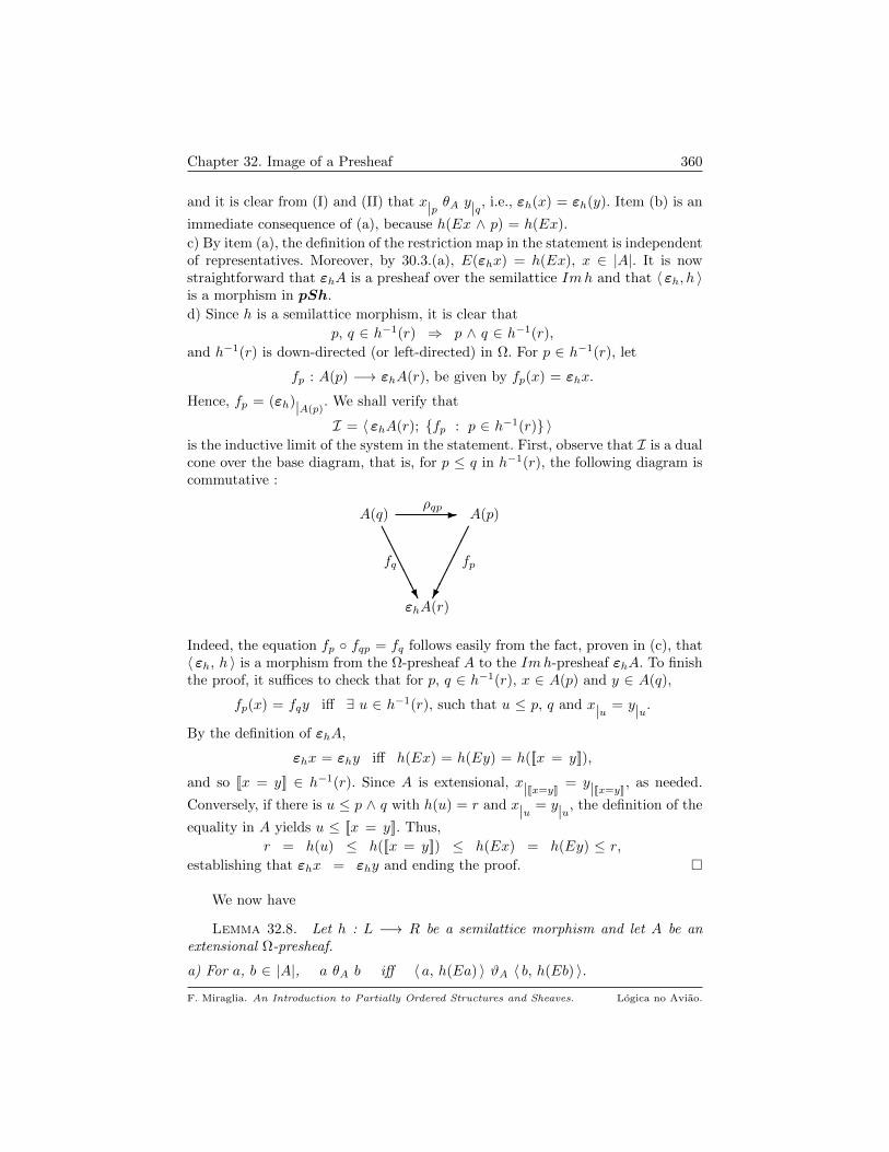
Chapter 32. Image of a Presheaf 360
and it is clear from (I) and (II) that x|p θA y|q, i.e., εh(x) = εh(y). Item (b) is an
immediate consequence of (a), because h(Ex ∧ p) = h(Ex).
c) By item (a), the definition of the restriction map in the statement is independentof representatives. Moreover, by 30.3.(a), E(εhx) = h(Ex), x ∈ |A|. It is nowstraightforward that εhA is a presheaf over the semilattice Imh and that 〈 εh, h 〉is a morphism in pSh.
d) Since h is a semilattice morphism, it is clear that
p, q ∈ h−1(r) ⇒ p ∧ q ∈ h−1(r),
and h−1(r) is down-directed (or left-directed) in Ω. For p ∈ h−1(r), let
fp : A(p) −→ εhA(r), be given by fp(x) = εhx.
Hence, fp = (εh)|A(p). We shall verify that
I = 〈 εhA(r); fp : p ∈ h−1(r) 〉is the inductive limit of the system in the statement. First, observe that I is a dualcone over the base diagram, that is, for p ≤ q in h−1(r), the following diagram iscommutative :
A(q) - A(p)
fq fp
εhA(r)
ρqp
AAAAAU
Indeed, the equation fp fqp = fq follows easily from the fact, proven in (c), that〈 εh, h 〉 is a morphism from the Ω-presheaf A to the Imh-presheaf εhA. To finishthe proof, it suffices to check that for p, q ∈ h−1(r), x ∈ A(p) and y ∈ A(q),
fp(x) = fqy iff ∃ u ∈ h−1(r), such that u ≤ p, q and x|u = y|u.
By the definition of εhA,
εhx = εhy iff h(Ex) = h(Ey) = h([[x = y]]),
and so [[x = y]] ∈ h−1(r). Since A is extensional, x|[[x=y]]= y|[[x=y]]
, as needed.
Conversely, if there is u ≤ p ∧ q with h(u) = r and x|u = y|u, the definition of the
equality in A yields u ≤ [[x = y]]. Thus,
r = h(u) ≤ h([[x = y]]) ≤ h(Ex) = h(Ey) ≤ r,
establishing that εhx = εhy and ending the proof.
We now have
Lemma 32.8. Let h : L −→ R be a semilattice morphism and let A be anextensional Ω-presheaf.
a) For a, b ∈ |A|, a θA b iff 〈 a, h(Ea) 〉 ϑA 〈 b, h(Eb) 〉.
F. Miraglia. An Introduction to Partially Ordered Structures and Sheaves. Logica no Aviao.
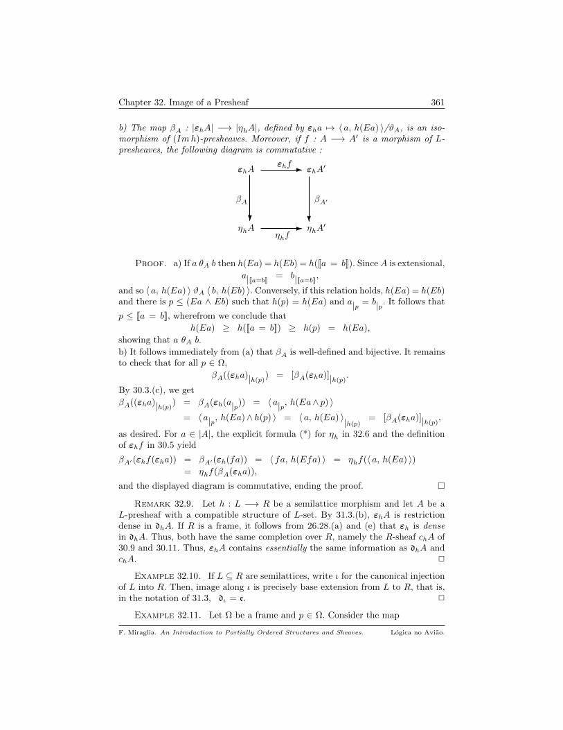
Chapter 32. Image of a Presheaf 361
b) The map βA : |εhA| −→ |ηhA|, defined by εha 7→ 〈 a, h(Ea) 〉/ϑA, is an iso-morphism of (Imh)-presheaves. Moreover, if f : A −→ A′ is a morphism of L-presheaves, the following diagram is commutative :
ηhA
εhA
?
- εhA′
βA
εhf
ηhA′
βA′
ηhf
?-
Proof. a) If a θA b then h(Ea) = h(Eb) = h([[a = b]]). Since A is extensional,
a|[[a=b]]= b|[[a=b]]
,
and so 〈 a, h(Ea) 〉 ϑA 〈 b, h(Eb) 〉. Conversely, if this relation holds, h(Ea) = h(Eb)and there is p ≤ (Ea ∧ Eb) such that h(p) = h(Ea) and a|p = b|p. It follows that
p ≤ [[a = b]], wherefrom we conclude that
h(Ea) ≥ h([[a = b]]) ≥ h(p) = h(Ea),
showing that a θA b.
b) It follows immediately from (a) that βA is well-defined and bijective. It remainsto check that for all p ∈ Ω,
βA((εha)|h(p)) = [βA(εha)]|h(p)
.
By 30.3.(c), we get
βA((εha)|h(p)) = βA(εh(a|p)) = 〈 a|p, h(Ea∧ p) 〉
= 〈 a|p, h(Ea)∧h(p) 〉 = 〈 a, h(Ea) 〉|h(p)= [βA(εha)]|h(p)
,
as desired. For a ∈ |A|, the explicit formula (*) for ηh in 32.6 and the definitionof εhf in 30.5 yield
βA′(εhf(εha)) = βA′(εh(fa)) = 〈 fa, h(Efa) 〉 = ηhf(〈 a, h(Ea) 〉)= ηhf(βA(εha)),
and the displayed diagram is commutative, ending the proof.
Remark 32.9. Let h : L −→ R be a semilattice morphism and let A be aL-presheaf with a compatible structure of L-set. By 31.3.(b), εhA is restrictiondense in dhA. If R is a frame, it follows from 26.28.(a) and (e) that εh is densein dhA. Thus, both have the same completion over R, namely the R-sheaf chA of30.9 and 30.11. Thus, εhA contains essentially the same information as dhA andchA. 2
Example 32.10. If L ⊆ R are semilattices, write ι for the canonical injectionof L into R. Then, image along ι is precisely base extension from L to R, that is,in the notation of 31.3, dι = e. 2
Example 32.11. Let Ω be a frame and p ∈ Ω. Consider the map
F. Miraglia. An Introduction to Partially Ordered Structures and Sheaves. Logica no Aviao.

Chapter 32. Image of a Presheaf 362
h : Ω −→ p← given by h(u) = p ∧ u.
The ideal p← is a frame and h is a surjective [∧
,∨
]-morphism. If X is a topologicalspace and U is an open set in X, then h corresponds to the dual of the canonicalcontinuous injection of U into X 3.
I. If A is an extensional presheaf over Ω, then εhA is an extensional presheaf overp←. To describe the sections of εhA, let q ≤ p. Then,
h−1(q) = u ∈ Ω : u ∧ p = qand so q = min h−1(q). Consequently, 32.7.(d) yields
εhA(q) = lim→u∈h−1(q)A(u) = A(q).
Hence, image along h “forgets” the part of A that is outside p. Note that for alls, t ∈ |A|,
[[εhs = εht]] = p ∧ [[s = t]].
Thus, if Es, Et ∈ p←, εhs = εht iff s = t, whence εh is injective whenrestricted to the subset
⋃q≤p A(q) of |A|.
II. By 7.8, h has a right adjoint ρ : p← −→ Ω, determined by the adjunction
For all 〈u, q 〉 ∈ Ω × (p←), u ∧ p ≤ q iff u ≤ ρ(q).
Thus, [→] in 6.1 implies that for all q ≤ p, ρ(q) = (p → q).
Since h is surjective, by 7.9.(a), ρ is injective. Recalling that for all q ∈ p←
(p → ⊥) = ¬ p ≤ (p → q) ≤ (p → p) = >,
we get min(Imρ) = ¬ p, max(Imρ) = > and Imρ ⊆ (¬ p)→. In general, thelatter containment is strict : for instance, in the algebra of opens of (0, 1) ⊆ R, ifp = (0, 1/2) ∪ (1/2, 1), then ¬ p = ∅, but p is not of the form (p → q), q ≤ p.
If B is an extensional p←-set, then ερB is the Ω-set defined by
(i) |ερB| = |B|;(ii) For s, t ∈ |B|, [[s = t]]ερB = p → ([[s = t]]B) ≥ ¬ p.Thus, a section of extent q ≤ p in B, is considered as a section of extent (p → q)in the Ω-set ερB. In particular,
∗ A global section in B (of extent p) is a global section (of extent >) in ερB;
∗ The unique section over ⊥ in B, yields the unique section of extent ¬ p in ερB.
Thus, image along g “spreads out” B over Ω, without producing sections of extentstrictly less than ¬ p.
Now suppose that B is an extensional presheaf over p←. Then, by 32.7, ερB isa presheaf over Imρ. If q ≤ r ≤ p, the restriction map of B is transferred directlyto ερB, that is, if s ∈ ερB(ρ(r)), then
s|ρ(q) = s|q,regarded as an element of ερB(ρ(q)). We take the opportunity to comment on theextension of ερB to the Ω-presheaf dρB, discussed in 31.3. For u ∈ Ω,
3That is, h = ι∗, where ι : U → X.
F. Miraglia. An Introduction to Partially Ordered Structures and Sheaves. Logica no Aviao.
Chapter 32. Image of a Presheaf 363
G(u) = q ∈ p← : u ≤ (p → q) = q ∈ p← : u ∧ p ≤ q= q ≤ p : h(u) ≤ q.
and dρB(u) = lim→q∈G(u)B(q). Since for all u ∈ Ω, G(u) = G(p ∧ u) and
(p ∧ u) ∈ p←, it follows that 4
dρB(u) = dρB(p ∧ u) = lim→p∧u≤q≤pB(q) = B(p ∧ u).
This fits well with the preceding results because if u = (p → q), then
p ∧ u = p ∧ (p → q) = p ∧ q = q,
whence dρB(p → q) = B(q). If v ≤ u in Ω, the restriction map from dρB(u) todρB(v) is induced by B, i.e., if s ∈ dρB(u) = B(p ∧ u), then s|v in |dρB| is s|p∧vin |B|. Therefore,
∗ (dρB)|p is a copy of B, that is, for all r, q ≤ p,
dρB(q) = B(q) and ·|q is the restriction map of B;
∗ If u ≤ ¬ p, then dρB(u) = B(⊥) and the restriction maps into dρB(u) are theonly possible ones, taking all elements to ∗;∗ If s ∈ dρB(u) and t ∈ dρB(v), then
[[s = t]]dρB = u ∧ v ∧ ρ([[s = t]]B),
the verification of which is left to the reader.
∗ εhερB = B.
III. By 7.8, h has a left adjoint, λ : p← −→ Ω, determined by the adjunction
For all 〈x, q 〉 ∈ p← × Ω, λ(x) ≤ q iff x ≤ h(q) = p ∧ q.Hence, λ is the natural inclusion x ∈ p← 7−→ x ∈ Ω.
If D is an extensional p←-set then ελD is the extensional Ω-set, whose domainis that of D and whose equality is [[∗ = ∗]]D, considered as an element of Ω. In thiscase, ελA may be identified with A, equality included.
If D is a p←-presheaf, as observed in 32.10, dλ is base extension from p← toΩ. To describe the sections of dλD = eD, let u ∈ Ω. Then,
G(u) = q ∈ p← : u ≤ q =
u← if u ∈ p←
∅ otherwise.
Therefore,
eD(u) =
D(u) if u ≤ p
∅ otherwise,
with restriction induced by D. Therefore, eD is a copy of D over the elements inp←, with empty set of sections over all elements of Ω outside p←. If A is a presheafover Ω, the reader can check that the preceding description and the results in (I)above entail
4Or put differently, since u ≤ (p → (p ∧ u)), p ∧ u = min(G(u)) ∈ p←.
F. Miraglia. An Introduction to Partially Ordered Structures and Sheaves. Logica no Aviao.
Chapter 32. Image of a Presheaf 364
dλεhA = edhA = A|p.The examples above are a special − although important −, instances of 30.12
and 33.9. 2
The description of the base extension along the natural embedding p← → Ωin 32.11.(III) yields
Corollary 32.12. Let Ω be frame and p ∈ Ω. If A is a sheaf over p←, theneA is a sheaf over Ω, such that for u ∈ Ω
eA(u) =
A(u) if u ≤ p
∅ otherwise.2
Exercises
32.13. Let Lh−→ R be a semilattice morphism, A be a L-presheaf and r ∈
Imh.
a) h−1(r) is a down-directed subset of L.
b) For u ≤ v in h−1(r), let ρuv : A(u) −→ A(v) be the restriction map of A. Thesystem 〈A(u); ρuv : v ≤ u in h−1(r) 〉 is inductive and
ηhA(r) = lim→u∈h−1(r)A(u). 2
32.14. Show that Proposition 30.12 holds for the image functor, that is, if
Lf−→ R
g−→ T are semilattice morphisms, then dg f = dg df . 2
32.15. 5 Let h : Ω −→ R be a surjective semilattice morphism and let C(R) bethe category whose objects are extensional R-presheaves with compatible structureof R-set and arrows R-set morphisms. By 32.7.(c), εh is a functor from pSh(Ω)to C(R). Prove that this functor preserves all finite limits. 2
5This exercise complements 30.6.
F. Miraglia. An Introduction to Partially Ordered Structures and Sheaves. Logica no Aviao.
CHAPTER 33
Inverse Image of a Presheaf
Let h : L −→ R be a semilattice morphism. If B is a R-presheaf, set
(i) |ihB| =∐p∈L B(h(p)) =
⋃p∈L B(h(p)) × p;
(ii) EηhB〈 s, p 〉 = p; (iii) 〈 s, p 〉|q = 〈 s|h(q), p ∧ q 〉.
The properties [rest 1] − [rest 3] in 26.1 are readily verified. For instance
〈 s, p 〉|p = 〈 s|h(p), p 〉 = 〈 s, p 〉,
because s ∈ B(h(p)) and B is a R-presheaf. Similarly, for p, q, r ∈ L,
(〈 s, p 〉|q)|r = 〈 (s|h(q))|h(r)
, p∧ q ∧ r 〉 = 〈 s|h(q)∧h(r), p∧ q ∧ r 〉
= 〈 s|h(q∧r), p∧ q ∧ r 〉 = 〈 s, p 〉|q∧r.
Definition 33.1. The presheaf ihB is the inverse image of B along h.
Remark 33.2. As was the case in 30.13, for sheaves over topological spaces,classical nomenclature is dual to ours. If f : X −→ Y is a continuous map and Ais a sheaf over X, inverse image along f∗ is called image along f , written f∗A.The arguments for this and for our usage are the same as in 30.13. Additionalarguments will emerge in 33.9. A clue to what is happening is already in 33.11. 2
Proposition 33.3. Let h : L −→ R be a semilattice morphism and B aR-presheaf.
a) ihB is extensional whenever h is a [∧,∨
]-morphism and B is extensional.
b) The map
ih : |ihB| −→ |B|, given by 〈 s, p 〉 7→ s,
makes 〈 ih, h 〉 a morphism from ihB to B in pSh (29.1.(b)), with the followinguniversal property :
If A is a L-presheaf and 〈 f, h 〉 : A −→ B is a morphism in pSh, there is aunique morphism of L-presheaves, g : A −→ ihB, making the following diagramcommutative :
365

Chapter 33. Inverse Image of a Presheaf 366
A - ihB
〈 f, h 〉 〈 ih, h 〉
B
〈 g, IdL 〉
AAAAAAU
c) If L and R are frames, h is a frame morphism and B is a sheaf, then ihB is asheaf over L.
Proof. a) For 〈 s, p 〉, 〈 t, p 〉 ∈ |ihB|, suppose that there is α ⊆ L is such that∨α = p and 〈 s|t(q), q 〉 = 〈 t|h(q)
, q 〉, for all q ∈ α.
Since h preserves joins, we have∨q∈α h(q) = h(p) and s|h(q)
= t|h(q), for all
q ∈ α. Since EBs = EBt = h(p), the extensionality of B implies that s = t andso 〈 s, p 〉 = 〈 t, p 〉, as needed.
b) Clearly, 〈 ih, h 〉 is a morphism in pSh. If 〈 f, h 〉 : A −→ B is a morphism inpSh, then for all x ∈ |A|, we have EBfx = h(EAx). Hence, 〈 fx,EAx 〉 ∈ |ihB|,and the map
g : |A| −→ |ihB|, given by by x 7−→ 〈 fx,EAx 〉is well-defined. If p ∈ L and x ∈ |A|, we have
g(x|p) = 〈 f(x|p), p ∧ EAx 〉 = 〈 (fx)|h(p), p ∧ EAx 〉 = 〈 fx,EAx 〉|p
= (gx)|p,
and g is a morphism of L-presheaves. Uniqueness is clear.
c) Let 〈xi, pi 〉 : i ∈ I be a compatible set of sections in ihB, i.e., for all i, j ∈ I〈xi, pi 〉|pj
= 〈xi|h(pj), pi ∧ pj 〉 = 〈xj |h(pj)
, pi ∧ pj 〉 = 〈xj , pj 〉|pi.
Consequently, xi|h(pj)= xj |h(pi)
; since EBxi = h(pi), the collection xi, i ∈ I,
is compatible in B. Let x be the unique gluing of the xi in B. Since h preservesjoins, it follows that
EBx =∨i∈I h(pi) = h(
∨i∈I pi),
and so 〈x, q 〉, with q =∨i∈I pi, is an element in the domain of ihB. It is easily
established that 〈x, q 〉 is a gluing of the 〈xi, pi 〉 in ihB. Uniqueness of 〈x, q 〉 is aconsequence of item (a), ending the proof.
Illustrating the interplay between direct and inverse image we have
F. Miraglia. An Introduction to Partially Ordered Structures and Sheaves. Logica no Aviao.
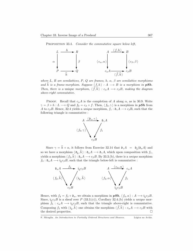
Chapter 33. Inverse Image of a Presheaf 367
Proposition 33.4. Consider the commutative square below left,
P
L
?
- R
α
h
Q
β
h
?- cαA
A
?
- B
〈 cα, α 〉
〈 f, h 〉
cβB
〈 cβ , β 〉
〈 f , h 〉
?-
where L, R are semilattices, P , Q are frames, h, α, β are semilattice morphisms
and h is a frame-morphism. Suppose 〈 f, h 〉 : A −→ B is a morphism in pSh.
Then, there is a unique morphism, 〈 f , h 〉 : cαA −→ cβB, making the diagramabove-right commutative.
Proof. Recall that cαA is the completion of A along α, as in 30.9. Writeγ = β h : L −→ Q and f0 = cβ f . Then, 〈 f0, γ 〉 is a morphism in pSh fromA to cβB. Hence, 32.4 yields a unique morphism, f1 : dγA −→ cβB, such that thefollowing triangle is commutative :
A - dγA
〈 f0, γ 〉 f1
cβB
〈 dγ , γ 〉
AAAAAU
Since γ = h α, it follows from Exercise 32.14 that dγA = dh(dαA) and
so we have a morphism 〈 dh, h 〉 : dαA −→ dγA, which upon composition with f1,
yields a morphism 〈 f2, h 〉 : dαA −→ cβB. By 33.3.(b), there is a unique morphismf3 : dαA −→ ihcβB, such that the triangle below-left is commutative :
dαA - ihcβB
〈 f2, h 〉 〈 ih, h 〉
cβB
f3
AAAAAU
A - cαA
〈 f4, α 〉 f5
ihcβB
〈 cα, α 〉
AAAAAU
Hence, with f4 = f3 dα, we obtain a morphism in pSh, 〈 f4, α 〉 : A −→ ihcβB.Since, ihcβB is a sheaf over P (33.3.(c)), Corollary 32.4.(b) yields a unique mor-phism f5 : cαA −→ ihcβB, such that the triangle above-right is commutative.
Composing f5 with 〈 ih, h 〉 one obtains the morphism 〈 f , h 〉 : cαA −→ cβB withthe desired properties.
F. Miraglia. An Introduction to Partially Ordered Structures and Sheaves. Logica no Aviao.
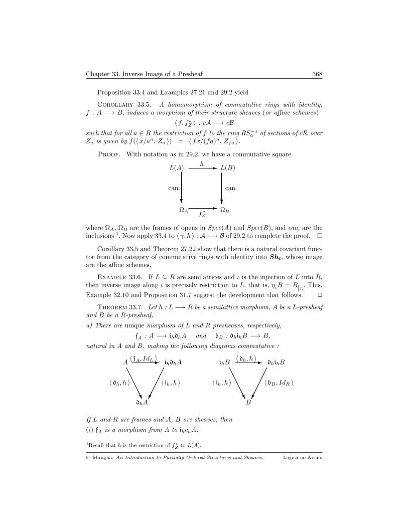
Chapter 33. Inverse Image of a Presheaf 368
Proposition 33.4 and Examples 27.21 and 29.2 yield
Corollary 33.5. A homomorphism of commutative rings with identity,f : A −→ B, induces a morphism of their structure sheaves (or affine schemes)
〈 f, f∗Z 〉 : cA −→ cBsuch that for all a ∈ R the restriction of f to the ring RS−1
a of sections of cR overZa is given by f(〈x/an, Za 〉) = 〈 fx/(fa)n, Zfa 〉.
Proof. With notation as in 29.2, we have a commutative square
ΩA
L(A)
?
- L(B)
can.
h
ΩB
can.
f∗Z
?-
where ΩA, ΩB are the frames of opens in Spec(A) and Spec(B), and can. are theinclusions 1. Now apply 33.4 to 〈 γ, h 〉 : A −→ B of 29.2 to complete the proof.
Corollary 33.5 and Theorem 27.22 show that there is a natural covariant func-tor from the category of commutative rings with identity into Sht, whose imageare the affine schemes.
Example 33.6. If L ⊆ R are semilattices and ι is the injection of L into R,then inverse image along ι is precisely restriction to L, that is, ηιB = B|L. This,
Example 32.10 and Proposition 31.7 suggest the development that follows. 2
Theorem 33.7. Let h : L −→ R be a semilattice morphism, A be a L-presheafand B be a R-presheaf.
a) There are unique morphism of L and R presheaves, respectively,
fA : A −→ ihdhA and bB : dhihB −→ B,
natural in A and B, making the following diagrams commutative :
A - ihdhA
〈 dh, h 〉 〈 ih, h 〉
dhA
〈 fA, IdL 〉
AAAAAU
ihB - dhihB
〈 ih, h 〉 〈 bB , IdR 〉
B
〈 dh, h 〉
AAAAAU
If L and R are frames and A, B are sheaves, then
(i) fA is a morphism from A to ihchA;
1Recall that h is the restriction of f∗Z to L(A).
F. Miraglia. An Introduction to Partially Ordered Structures and Sheaves. Logica no Aviao.
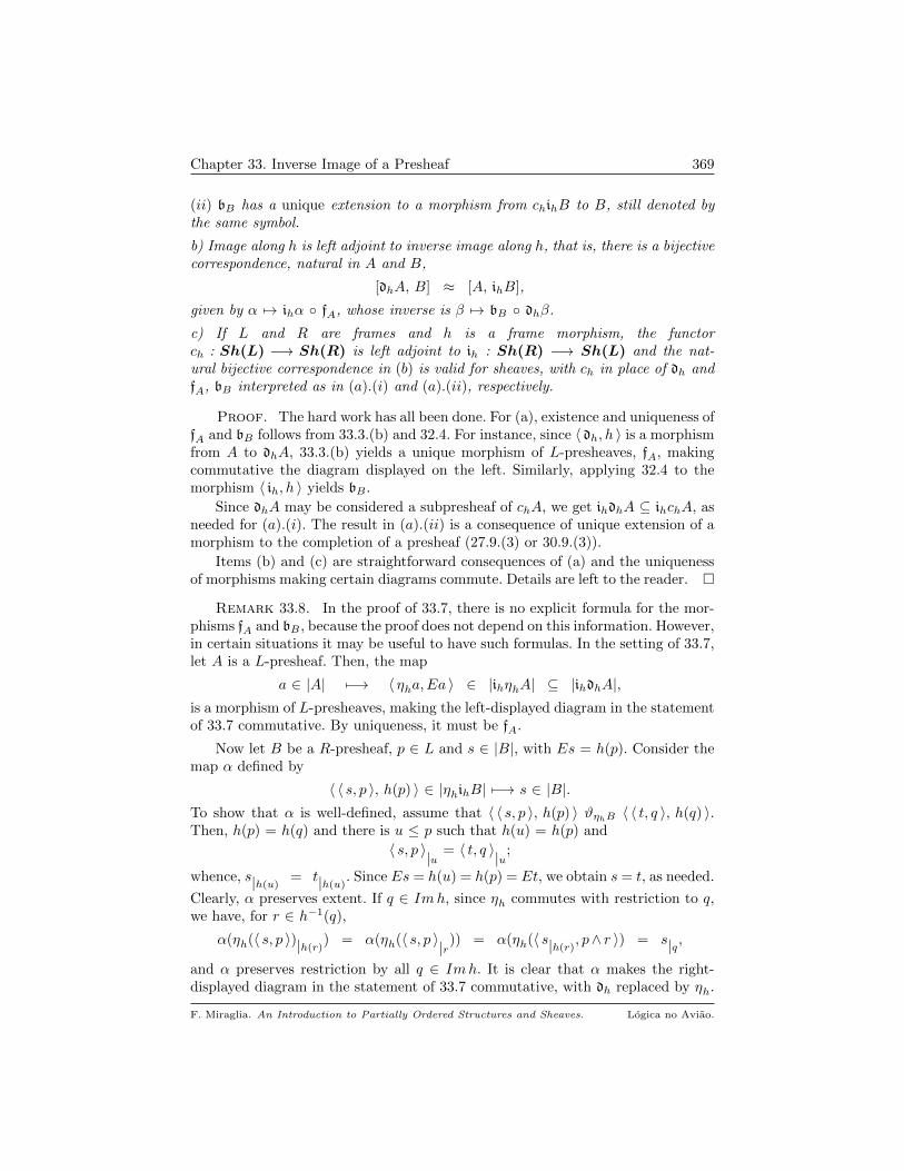
Chapter 33. Inverse Image of a Presheaf 369
(ii) bB has a unique extension to a morphism from chihB to B, still denoted bythe same symbol.
b) Image along h is left adjoint to inverse image along h, that is, there is a bijectivecorrespondence, natural in A and B,
[dhA, B] ≈ [A, ihB],
given by α 7→ ihα fA, whose inverse is β 7→ bB dhβ.
c) If L and R are frames and h is a frame morphism, the functorch : Sh(L) −→ Sh(R) is left adjoint to ih : Sh(R) −→ Sh(L) and the nat-ural bijective correspondence in (b) is valid for sheaves, with ch in place of dh andfA, bB interpreted as in (a).(i) and (a).(ii), respectively.
Proof. The hard work has all been done. For (a), existence and uniqueness offA and bB follows from 33.3.(b) and 32.4. For instance, since 〈 dh, h 〉 is a morphismfrom A to dhA, 33.3.(b) yields a unique morphism of L-presheaves, fA, makingcommutative the diagram displayed on the left. Similarly, applying 32.4 to themorphism 〈 ih, h 〉 yields bB .
Since dhA may be considered a subpresheaf of chA, we get ihdhA ⊆ ihchA, asneeded for (a).(i). The result in (a).(ii) is a consequence of unique extension of amorphism to the completion of a presheaf (27.9.(3) or 30.9.(3)).
Items (b) and (c) are straightforward consequences of (a) and the uniquenessof morphisms making certain diagrams commute. Details are left to the reader.
Remark 33.8. In the proof of 33.7, there is no explicit formula for the mor-phisms fA and bB , because the proof does not depend on this information. However,in certain situations it may be useful to have such formulas. In the setting of 33.7,let A is a L-presheaf. Then, the map
a ∈ |A| 7−→ 〈 ηha,Ea 〉 ∈ |ihηhA| ⊆ |ihdhA|,is a morphism of L-presheaves, making the left-displayed diagram in the statementof 33.7 commutative. By uniqueness, it must be fA.
Now let B be a R-presheaf, p ∈ L and s ∈ |B|, with Es = h(p). Consider themap α defined by
〈 〈 s, p 〉, h(p) 〉 ∈ |ηhihB| 7−→ s ∈ |B|.To show that α is well-defined, assume that 〈 〈 s, p 〉, h(p) 〉 ϑηhB 〈 〈 t, q 〉, h(q) 〉.Then, h(p) = h(q) and there is u ≤ p such that h(u) = h(p) and
〈 s, p 〉|u = 〈 t, q 〉|u;
whence, s|h(u)= t|h(u)
. Since Es = h(u) = h(p) = Et, we obtain s = t, as needed.
Clearly, α preserves extent. If q ∈ Imh, since ηh commutes with restriction to q,we have, for r ∈ h−1(q),
α(ηh(〈 s, p 〉)|h(r)) = α(ηh(〈 s, p 〉|r)) = α(ηh(〈 s|h(r)
, p∧ r 〉) = s|q,
and α preserves restriction by all q ∈ Imh. It is clear that α makes the right-displayed diagram in the statement of 33.7 commutative, with dh replaced by ηh.
F. Miraglia. An Introduction to Partially Ordered Structures and Sheaves. Logica no Aviao.
Chapter 33. Inverse Image of a Presheaf 370
By 31.3.(d), α has a unique extension to a morphism from dhihB to B. Thisextension makes the right-displayed diagram in the statement of 33.7 commute,and so is the required morphism bB . 2
In the spatial setting, if f : X −→ Y is a continuous map, then f∗ is a framemorphism, with right adjoint f∗. We now consider an abstract counterpart of thissituation, already previewed in 32.11.
As shown by (a) and (d) in 33.3, inverse image has pleasant preservationproperties when h is a [∧,
∨]-morphism. Additionally, 7.8 guarantees that h has
a right adjoint, g : R −→ L, that is, g is a∧
-morphism such that
[adj] For all 〈u, v 〉 ∈ L × R, hu ≤ v ⇔ u ≤ gv.
When L and R are frames, there is a connection between the inverse image alongh and the image along g, for extensional presheaves :
Theorem 33.9. Let h : L −→ R be a frame morphism, with right adjoint g.Let A, B be an extensional presheaves over L and R, respectively. Then,
a) For all 〈 s, p 〉, 〈 t, q 〉 ∈ |ihB|[[〈 s, p 〉 = 〈 t, q 〉]] = g([[s = t]]B) ∧ p ∧ q.
b) There is an injective L-set morphism, natural in B,
ιB : εgB −→ ihB, given by εgs 7−→ 〈 s|hg(Es), g(Es) 〉,
whose image is restriction dense 2 in ihB. Furthermore, if p ∈ Img and x ∈ |εgB|,then ιB(x|p) = ιB(x)|p.
c) If B is a R-sheaf, ιB has a unique extension to a natural isomorphism fromcgB to ihB, that in turn induces a natural isomorphism between the functors cgand ih.
d) The functor ch is left adjoint to cg.
e) If h is surjective, then
(1) chihB ≈ chcgB ≈ B;
(2) The map 〈 ih, h 〉 : ihεhA −→ εhA is a retract (29.5).
f) If h is injective, then ihchA ≈ cgchA ≈ A.
Proof. a) Since E〈 s, p 〉 = p in ihB, while EBs = h(p), we have
[[〈 s, p 〉 = 〈 t, q 〉]] =∨u ≤ p ∧ q : 〈 s, p 〉|u = 〈 t, q 〉|u
=∨u ≤ p ∧ q : 〈 s|h(u)
, u 〉 = 〈 t|h(u), u 〉
=∨u ≤ p ∧ q : s|h(u)
= t|h(u)
=∨u ≤ p ∧ q : h(u) ≤ [[s = t]]B,
where the last step in the above equalities follows from extensionality and 26.8.(d).(2).Since h preserves arbitrary joins, it follows that
2Defined in 26.28.(d).
F. Miraglia. An Introduction to Partially Ordered Structures and Sheaves. Logica no Aviao.
Chapter 33. Inverse Image of a Presheaf 371
h([[〈 s, p 〉 = 〈 t, q 〉]]) ≤ [[s = t]]B ,
and the adjointness relation [adj], E〈 s, p 〉 = p and E〈 t, q 〉 = q, entail
[[〈 s, p 〉 = 〈 t, q 〉]] ≤ g([[s = t]]B) ∧ p ∧ q.Let w = g([[s = t]]B) ∧ p ∧ q; clearly, h(w) ≤ h(p ∧ q) = h(p) ∧ h(q). By 7.8.(a),we have
For all v ∈ R and p ∈ L, hg(v) ≤ v and p ≤ gh(p), (*)
Thus,
h(w) = h(g([[s = t]]B) ∧ p ∧ q) = h(g([[s = t]]B)) ∧ h(p) ∧ h(q)
≤ [[s = t]]B ∧ h(p) ∧ h(q) = [[s = t]]B ,
and so s|h(w)= t|h(w)
in B. Hence,
〈 s, p 〉|w = 〈 s|h(w), w 〉 = 〈 t|h(w)
, w 〉 = 〈 t, q 〉|w,
showing that w ≤ [[〈 s, p 〉 = 〈 t, q 〉]], as needed.
b) For s ∈ |B|, (*) entails h(g(Es)) ≤ Es and so 〈 s|hg(Es), g(Es) 〉 is in |ihA|. To
show that ιB is well-defined, let t ∈ |B| verify εgs = εgt; then
g(Es) = g(Et) = g([[s = t]])
and so h(g([[s = t]])) ≤ [[s = t]] ((*), again), which entails s|hg(Es) = t|hg(Et), as
needed. Clearly,
EιBεgs = g(Es) = Eεgs.
Furthermore, item (a) yields
[[ιBεgs = ιBεgt]] = [[〈 s|hg(Es), g(Es) 〉 = 〈 t|hg(Et), g(Et) 〉]]
= g([[s|hg(Es) = 〈 t|hg(Et) 〉]]) ∧ g(Es) ∧ g(Et)
= g([[s = t]]) ∧ g(Es) ∧ g(Et)
= g([[s = t]]) = [[εgs = εgt]],
and ιB is, by 25.21, a monic morphism from εGB into ihB. For 〈 s, p 〉 ∈ |ihB|, wehave, because of Es = h(p) and hgh = h (7.8.(b)),
ξ =def ιBεgs = 〈 s|hg(Es), g(Es) 〉 = 〈 s|hgh(p)
, gh(p) 〉= 〈 s|h(p)
, gh(p) 〉 = 〈 s, gh(p) 〉,
and so, since p ≤ gh(p), it follows that
ξ|p = 〈 s|h(p), p ∧ gh(p) 〉 = 〈 s, p 〉.
Hence, the image of ιB is restriction dense (26.28.(d)) in ihB. Similar techniqueswill establish the remaining statements in (b).
c) By 27.17, ιB has a unique monic extension, γB , to cgB, the completion of εgBover L. Since the image of ιB is restriction dense in ihB, it is clear that γB is onto|ihB|, and hence an isomorphism. Just as in the proof of 30.12, the family
γ = γB : B is a R-sheafis a natural isomorphism between the functors cg and ih. Hence, sheaf-theoreticalinverse image by h comes to the same thing as sheaf-theoretical image by its adjoint
F. Miraglia. An Introduction to Partially Ordered Structures and Sheaves. Logica no Aviao.
Chapter 33. Inverse Image of a Presheaf 372
g. This also establishes (d). For (e), observe that if h is surjective, 7.9 guaranteesthat h g = IdR and (1) is an immediate consequence of (b) and 30.12.(c). For(2), consider the morphism
〈 ι(εhA) εg, g 〉 : εhA −→ ihεhA,
where ι∗ is defined in item (b). Since h g = IdR, it remains to check that(ih ι(εhA) εg) is the identity in εhA. The definitions of ι∗ in item (b) and of ihin 33.3.(b) yield, for x ∈ |A|,
ih(ι(εhA)(εg(εhx))) = ih
(〈 (εhx)|hg(Ex)
, g(Eεhx) 〉)
= ih(〈 εhx, g(Eεhx) 〉) = εhx,
as needed. Item (f) is similar to (e).(1), ending the proof.
The reader will have noticed that Propositions 30.12 and Theorem 33.9 ap-ply to the spatial situation, in fact generalizing it considerably. All the classicalrelations involving image and inverse image along a continuous map are straight-forward consequences of the results presented above.
Example 33.10. Let h : Ω −→ 2 = ⊥, > be a pure state in Ω (12.14), i.e.,a surjective frame morphism; h has a right adjoint g (7.8), given by
g(>) = > and g(⊥) =∨p ∈ Ω : h(p) = ⊥.
Since F = coker h = q ∈ Ω : h(q) = > is a completely prime filter in Ω (12.1),the join of all elements outside F is outside F , constituting the value of g at ⊥.Write
qF = g(⊥) =∨p ∈ Ω : p 6∈ F.
In the spatial setting, if X is a topological space and x is point in X, the(completely prime) filter of open neighborhoods of x in X induces a pure state pxin Ω(X), given by
px(U) = > iff u ∈ νx.
The right adjoint of px takes ⊥ to (X − x), the largest open in X to whichx does not belong. If B is a set (i.e., a 2-sheaf), inverse image of B along h is,by 33.3.(c), a sheaf over Ω, which by 33.9.(c), is the same as the completion ofεgB. We discuss both constructions, to illustrate the relations between them. Oneshould keep in mind that, as a 2-sheaf, the domain of B is B ∪ ∗, where ∗ 6∈ B,with equality given by
[[x = y]] =
> if x = y in B,
⊥ otherwise.
In particular, [[∗ = ∗]] = [[x = ∗]] = ⊥.
The Ω-set εgB has sections only over g(⊥) = qF and g(>) = >, as follows :
εGB(>) = B and εGB(qF ) = ∗.Moreover, since εg is injective and B is extensional, we may identify εGx withx ∈ |B| (30.2). Thus, for x, y ∈ |εgB|,
F. Miraglia. An Introduction to Partially Ordered Structures and Sheaves. Logica no Aviao.

Chapter 33. Inverse Image of a Presheaf 373
(I) [[x = y]]εgB = g([[x = y]]) =
> if x = y in B;
qF otherwise.
The definition in the first paragraph of this Chapter yields, since B(⊥) = ∗,|ihB| =
⋃p∈Ω B(h(p)) × p
=⋃p∈F B × p ∪
⋃p≤qF ∗ × p.
ihB is a sheaf over Ω, the skyscraper sheaf over Ω, centered at F andgenerated by B.
Note that εgB is indeed restriction dense in ihB and so the latter is the former’scompletion. In view of 33.9.(a) and (I) above, equality in ihB is given by
[[〈x, p 〉 = 〈 y, q 〉]] = p ∧ q ∧ g([[x = y]])
=
p ∧ q if x = y in B,
p ∧ q ∧ qF otherwise.
It is instructive to go back to the spatial setting and to verify, directly, that ihBis a sheaf. 2
Exercises
33.11. In the setting of 32.11, show that if B is a p←-presheaf, then dgB canbe naturally identified with ihB
3. 2
33.12. Let h : L −→ R be a semilattice morphism and B a flabby R-presheaf(26.28.(e)). Then, ihB is a flabby L-presheaf. 2
33.13. If Lh−→ R
k−→ T are semilattice morphisms, then ikh = ih ik. 2
3So inverse image along h is image along g.
F. Miraglia. An Introduction to Partially Ordered Structures and Sheaves. Logica no Aviao.
CHAPTER 34
Localization, Fibers and Stalks
As an application of the image functor, we present the notions of localization,fiber and stalk.
Definition 34.1. Let L be a distributive lattice and F a proper filter in L.Let πF : L −→ L/F be the natural quotient map. If A is a L-set, write
A/F =def επFA
for the extensional image of A along πF (30.4). The L/F -set A/F is the local-ization of A at F ; its set of global sections is the fiber of A at F , written AF .The morphism
〈 εF , πF 〉 =def 〈 επF , πF 〉 : A −→ A/F
is the localization morphism of A at F . Whenever context allows, write x/Ffor εFx, x ∈ |A|. If u ∈ F and s ∈ A(u), then εF s is a global section of A/F 1,written sF and called the germ of s at F 2.
If f : A −→ B is a morphism of L-sets, write
f/F : A/F −→ B/F ,
for the morphism επF f (the localization of f at F ) and fF for the map induced byf/F on global sections (the fiber map induced by f at F ).
Remark 34.2. Recall that for a ∈ L, a/F stands for the equivalence class ofa by the congruence generated by F . By a standard abuse of notation, we have
a/F = π−1F (a/F ) and a/F = πF (a).
We collect here some of the formulas that describe explicitly the conceptsintroduced above. Let f : A −→ B be a morphism of L-sets and F a (proper)filter in L. For all x, y ∈ |A| :
(1)
[[x/F = y/F ]] = πF ([[x = y]]) = [[x = y]]/F ;
E(x/F ) = πF (Ex) = (Ex)/F ;
(2) f/F (x/F ) = (fx)/F ;
(3) [[f/F (x/F ) = f/F (y/F )]] = πF ([[fx = fy]]) = [[fx = fy]]/F .
(4) If Ex ∈ F , then fF (xF ) = f/F (x/F ) = (fx)/F = (fx)F , i.e., thegerm of a section at F is taken to the germ of fx at F .
1Recall that u ∈ F iff πF (u) = >.2By analogy with the classical construction; see 34.10.
374
Chapter 34. Localization, Fibers and Stalks 375
(5) If A is a L-presheaf, then A/F is a presheaf over L/F (32.7.(c)).
These observations will be used forthwith, without explicit reference. 2
Proposition 34.3. Let L be a distributive lattice. If A is a L-set and F is aproper filter in L, then for all x, y ∈ |A|a) If (Ex ∨ Ey) ∈ F , then x/F = y/F iff [[x = y]] ∈ F .
b) x/F ∈ AF iff Ex ∈ F . If Ex, Ey ∈ F , xF = yF iff [[x = y]] ∈ F .
c) If L is a Heyting algebra, x/F = y/F iff [x ≡ y] ∈ F 3.
Proof. Recall (4.9) that for p, q ∈ LπF p = πF q iff ∃ u ∈ F such that u ∧ p = u ∧ q. (*)
Since the equivalence relation θA defining |A/F | is given by
πF (Ex) = πF (Ey) = πF ([[x = y]]),
(*) and the fact that a filter is closed under meets yield
(**) x/F = y/F iff
∃ u ∈ F such that
u ∧ Ex = u ∧ Ey = u ∧ [[x = y]].
a) If (Ex ∨ Ey) ∈ F and x/F = y/F , there is u ∈ F verifying the conditions inthe right-hand side of (**). Hence,
(Ex ∨ Ey) ∧ u = (Ex ∧ u) ∨ (Ey ∧ u) = Ex ∨ u = u ∧ [[x = y]]
≤ [[x = y]],
and so [[x = y]] ∈ F . The converse is clear.
b) Since E(x/F ) = πF (Ex) and F = π−1F (>), it follows that x/F is a global section
of A/F iff Ex ∈ F . The remainder of (b) is an immediate consequence of (a).
c) If L is a HA and x/F = y/F , then (**) entails that for some u ∈ Fu ∧ (Ex ∨ Ey) = u ∧ [[x = y]] ≤ [[x = y]].
The adjunction [→] in 6.1 implies u ≤ [x ≡ y], and [x ≡ y] ∈ F . For the converse,28.2.(c) entails that, with u = [x ≡ y], the conditions in the right-hand side of(**) are satisfied, whence x/F = y/F .
For Ω-presheaves, the fiber construction is closer to its classical counterpart.From Propositions 34.3, 32.7 and 26.8 we obtain :
Corollary 34.4. If A is an extensional Ω-presheaf, then for all x, y ∈ |A|a) The following conditions are equivalent :
(1) x/F = y/F ; (2) [x ≡ y] ∈ F ; (3) ∃ p ∈ F with x|p = y|p.
b) E(x/F ) = > iff Ex ∈ F . If Ex, Ey ∈ F , then
xF = yF iff ∃ p ∈ F ∩ (Ex ∧ Ey)← such that x|p = y|p.
In particular, if p, Ex ∈ F , then (x|p)F = xF .
3For the definition of strict equality, [· ≡ ·], and its basic properties see 28.1 and 28.2.
F. Miraglia. An Introduction to Partially Ordered Structures and Sheaves. Logica no Aviao.
Chapter 34. Localization, Fibers and Stalks 376
c) For p ≤ q, let ρqp : A(q) −→ A(p) be the restriction map x 7→ x|p. For r ∈ Ω,
let Dr = q ∈ L : q ≤ r and q/F = r/F. The system
〈A(q); ρqp : p ≤ q with p, q in Dr 〉is an inductive system of sets and maps such that A/F (r/F ) = lim→q∈Dr
A(q).
In particular, AF = lim→p∈FA(p) i.e., the fiber of A at F is the inductive limit
of the sections with extent in F , by the restriction maps of A 4.
d) If B ⊆ |A| is restriction dense in A (26.28.(d)), then
AF = bF : b ∈ B and Eb ∈ F.If A is flabby (26.28.(e)), then AF = sF : s ∈ A(>).
Proof. We comment only on the first assertions in (c) and (d). By 30.3.(d),we have A/F (r/F ) = lim→q∈r/F
A(q). Since Dr is cofinal in r/F , the desired
conclusion follows from 17.15.(a). For (d), if p ∈ F and s ∈ A(p), there is x ∈ Bsuch that x|Es = s. By 34.3.(b), sF = xF .
Regarding completeness, we state
Lemma 34.5. Let F be a proper filter in the distributive lattice L. If A is afinitely complete L-set (25.34), then A/F is finitely complete over L/F .
Proof. By Exercise 26.29, A has a compatible structure of L-presheaf.Hence, A/F is a L/F -presheaf ((5) in 34.2) and to show that it is fc it is enoughto check that a finite compatible subset has a gluing.
Let T = s/F : s ∈ S be compatible in A/F , with S ⊆f |A|. This means thatfor s, s′ ∈ S,
πF (Es ∧ Es′) = πF ([[s = s′]]).
Relation (**) in the proof of 34.3 implies that for 〈 s, s′ 〉 ∈ S × S, there isu(s, s′) ∈ F , such that
(I) Es ∧ Es′ ∧ u(s, s′) = u(s, s′) ∧ [[s = s′]].
Since S is finite, u =∧s,s′∈S u(s, s′) ∈ F . Hence, (I) entails
∀ s, s′ ∈ S, Es ∧ Es′ ∧ u = u ∧ [[s = s′]],
i.e., the finite set s|u : s ∈ S is compatible in A. Since A is fc, there is t ∈ |A|,such that Et =
∨s∈S Es|u = u ∧
∨s∈S Es;
Es|u = [[t = s|u]] = u ∧ [[t = s]] = u ∧ Es.
Applying πF to these equations and recalling that u ∈ F , we obtain 5
E(t/F ) =∨s∈S E(s/F ) and ∀ s ∈ S, E(s/F ) = [[t/F = s/F ]],
whence t/F is the gluing of T in A/F , as needed.
4Generalizing the classical case of “stalks at a point in a topological space”.5The joins are finite and πF is a lattice morphism.
F. Miraglia. An Introduction to Partially Ordered Structures and Sheaves. Logica no Aviao.

Chapter 34. Localization, Fibers and Stalks 377
Example 34.6. Let A be a H-set (H a HA) and let D be the filter of denseelements in H (6.19). We know that H/D is a BA, isomorphic to the BA Reg(H)of regular elements in H (6.21). The localization at D furnishes a H/D-set, A/D,whose set of global sections, AD, is the fiber of A at D. If x, y ∈ |A| then it followsfrom 34.3.(c) and 6.8.(j) that
x/D = y/D iff ¬¬ [x ≡ y] ∈ D iff ¬¬ (Ex ∨ Ey) = ¬¬ [[x = y]].
In particular, if Ex, Ey ∈ D, then xF = yF iff ¬¬ [[x = y]] = >.
If A is a H-presheaf and p ∈ H, recall (6.19.(a)) that
D(p) = q ∈ H : p ≤ q ≤ ¬¬ pis the set of elements dense in p. Hence, 34.4.(c) entails
AD(p/D) = lim→q∈D(p)A(q).
In particular, AD = lim→d∈DA(d).
If A is finitely complete over H, 34.5 guarantees that A/D is finitely completeover H/D. We shall prove latter that if H is a frame and A is a sheaf over H, thenA/D is a sheaf over H/D (35.9).
Given the well-known connection between intuitionistic logic and Heyting alge-bras, on one hand, and classical logic and Boolean algebras, on the other, localiza-tion at D associates to the intuitionistic structure A, a “classical” structure, A/D.We shall explore this further, when discussing the regularization functor associatedto πD in 35.7. The reader might also consult [11] to see how this construction isconnected to the notion of ultrasheaf of first-order structures. 2
We now describe the concept of stalk.
Definition 34.7. Let L be a semilattice with > and 2 = ⊥,> be the 2-element Boolean algebra. Let h : L −→ 2 is a surjective semilattice morphism.If A is a L-set, the image of A along h is the stalk of A at h, written Ah. Iff : A −→ B is a morphism of L-set, write fh for the morphism εhf : Ah −→ Bh,called the stalk morphism induced by f at g. If s ∈ |A|, with h(Es) = >,write sh ∈ Ah for the germ of s at h.
Since the categories 2set, Sh(2), pSh(2) and Set are isomorphic, the stalkconstruction is a covariant functor from Lset to Set.
The next result shows that when L is a distributive lattice, stalk at h is nat-urally isomorphic to fiber at the cokernel of h.
Lemma 34.8. Let L be a distributive lattice and h : L −→ 2 a surjectivesemilattice morphism. Let A be a L-set and write F for coker h 6.
a) There is a unique semilattice morphism, g : L/F −→ 2, making the followingdiagram commutative, where πF is canonical quotient morphism from L to L/F :
6coker h = p ∈ L : h(p) = > is the cokernel of h; it is a proper filter in L.
F. Miraglia. An Introduction to Partially Ordered Structures and Sheaves. Logica no Aviao.
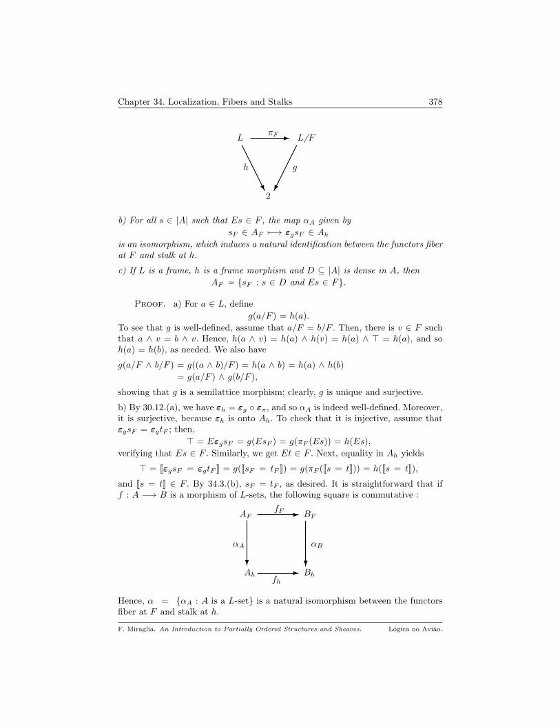
Chapter 34. Localization, Fibers and Stalks 378
L - L/F
h g
2
πF
AAAAAU
b) For all s ∈ |A| such that Es ∈ F , the map αA given by
sF ∈ AF 7−→ εgsF ∈ Ahis an isomorphism, which induces a natural identification between the functors fiberat F and stalk at h.
c) If L is a frame, h is a frame morphism and D ⊆ |A| is dense in A, then
AF = sF : s ∈ D and Es ∈ F.
Proof. a) For a ∈ L, define
g(a/F ) = h(a).
To see that g is well-defined, assume that a/F = b/F . Then, there is v ∈ F suchthat a ∧ v = b ∧ v. Hence, h(a ∧ v) = h(a) ∧ h(v) = h(a) ∧ > = h(a), and soh(a) = h(b), as needed. We also have
g(a/F ∧ b/F ) = g((a ∧ b)/F ) = h(a ∧ b) = h(a) ∧ h(b)
= g(a/F ) ∧ g(b/F ),
showing that g is a semilattice morphism; clearly, g is unique and surjective.
b) By 30.12.(a), we have εh = εg επ, and so αA is indeed well-defined. Moreover,it is surjective, because εh is onto Ah. To check that it is injective, assume thatεgsF = εgtF ; then,
> = EεgsF = g(EsF ) = g(πF (Es)) = h(Es),
verifying that Es ∈ F . Similarly, we get Et ∈ F . Next, equality in Ah yields
> = [[εgsF = εgtF ]] = g([[sF = tF ]]) = g(πF ([[s = t]])) = h([[s = t]]),
and [[s = t]] ∈ F . By 34.3.(b), sF = tF , as desired. It is straightforward that iff : A −→ B is a morphism of L-sets, the following square is commutative :
Ah
AF
?
- BF
αA
fF
Bh
αB
fh
?-
Hence, α = αA : A is a L-set is a natural isomorphism between the functorsfiber at F and stalk at h.
F. Miraglia. An Introduction to Partially Ordered Structures and Sheaves. Logica no Aviao.
Chapter 34. Localization, Fibers and Stalks 379
c) If h preserves joins, then F is completely prime, that is,∨i∈I pi ∈ F ⇒ ∃ i ∈ I with pi ∈ F .
To see this, suppose p =∨i∈I pi exists in L. Then,
> = h(p) = h(∨i∈I pi) =
∨i∈i h(pi).
It is immediate that the h(pi) cannot all be equal to ⊥. For x ∈ |A|, with Ex ∈ F ,we may write
Ex =∨d∈D [[x = d]],
and so there is d ∈ D such that [[x = d]] ∈ F . But then, Ed ∈ F and 34.3.(b)entails sF = dF , ending the proof.
Example 34.9. Let Ω be a frame and F a point (or completely prime filter)in Ω (12.1). The point F originates a pure state (12.14)
pF : Ω −→ 2, given by pF (p) = > iff a ∈ F .
However, 2 may be very far from the quotient Ω/F .
If A is a Ω-set, the stalk of A at pF is the image of A by pF . By Lemma 34.8,it is isomorphic to the fiber of A at F , but it will be important in applications toLogic to know that there is a frame morphism involved in the construction of AF .The isomorphism in 34.8 justifies the usage of “stalk” both for the fiber of A at Fand its image under pF . In Example 33.10 it was shown that inverse image alongpF corresponds to the construction known as the “skyscraper” sheaf.
To exemplify the concept in the spatial setting, let X be a topological spaceand x a point in X. Let f be the unique continuous map from ∅ into X, thattakes ∅ to x. Then, f∗ : Ω(X) −→ 2 is precisely the pure state associated to thecompletely prime filter νx, of open neighborhoods of x in X. Hence, in classicalnotation (30.13, 33.2)
∗ If A is a sheaf over X, f∗A is the stalk of A at the point x;
∗ If B is a set (i.e., a 2-sheaf), f∗B is the skyscraper sheaf on X, centered at xand generated by B. 2
Example 34.10. Let X be a topological space, A be Ω(X)-set and x ∈ X.Localizing A at the completely prime filter νx, yields an extensional (Ω(X)/νx)-set, A/νx, whose set of global sections is written Ax (the stalk of A at x); theelements of Ax are written sx. If s, t are sections in A such that Es, Et are openneighborhoods of x, then
sx = tx iff [[s = t]] ∈ νx.
If f , g are sections of the sheaf C(X,Y ) of 23.5, with Ef , Eg ∈ νx, then
fx = gx iff ∃ u ≤ Ef ∩ Eg such that f|u = g|u,
corresponding to the classical notion of stalk at x : f and g have the same germat x iff they coincide in an open neighborhood of x. Note that in the contextof Ω(X)-sets, there is more to this construction than just the stalk, even in theclassical setting, for we can consider the whole localization at x as a (Ω(X)/νx)-setin its own right. 2
F. Miraglia. An Introduction to Partially Ordered Structures and Sheaves. Logica no Aviao.

Chapter 34. Localization, Fibers and Stalks 380
Since a L-set is dense in its completion, 34.8.(c), 34.9 and 34.10 yield
Corollary 34.11. If F is a point in the frame Ω, then for all Ω-sets A
AF = (cA)F ,
where cA is the completion of A. In particular, if A is a presheaf over a topologicalspace X, the stalk of A and that of its completion are the same at all x ∈ X. 2
Example 34.12. Let L be a distributive lattice with ⊥ and >. Let U be amaximal filter in L. If a ∈ L, then
a/U = >/U or a/U = ⊥/U .
To see this, note that if U ∪ a has the fip 7, then a ∈ U , by maximality; otherwise,a is equivalent to ⊥ modulo U . Hence, the quotient L/U may be identified with2 = ⊥, >, and U originates a surjective lattice morphism
πU : L −→ 2, given by πU (a) = > iff a ∈ U .
There are many familiar constructions that are instances of “stalk at U”. Asan example, consider the sheaf M of 23.11 and 31.8; M is a flabby sheaf over L,that is, every section is the restriction of a global section in M (26.28.(e)).
Let U be an ultrafilter in L (i.e., an ultrafilter on I). By 34.4.(d), to computethe stalk of M at U it is enough to determine the germs of global section at U .For s, t ∈ M(I) =
∏i∈I Mi,
sU = tU iff [[s = t]] ∈ U iff i ∈ I : s(i) = t(i) ∈ U .
Thus, MU is the ultraproduct of the family Mi by the ultrafilter U . When U isa principal ultrafilter generated by i ∈ I,
U = u ⊆ I : i ∈ u,then MU can be canonically identified with Mi.
In 31.8 we described the extension ofM to a β I-sheaf, eM. Now, an ultrafilteron I is a point in the topological space βI. Furthermore, for every U ∈ Ω(βI),eM(U) =M(u), where u is the unique element of 2I such that U = Su. It followsthat the stalk of eM at a point U of βI is still the ultraproduct of the Mi at U .
If instead of an ultrafilter U on I, we had considered a filter F on I, thenthe fiber of M at F is the reduced product of the Mi by F , another importantconstruct in Model Theory. 2
Certain properties between Ω-presheaves are faithfully reflected by fiber andlocalization, as is the case for commutative rings 8. An example is Proposition34.13, proven below. Recall that S(L) is the Stone space of the distributive latticeL (19.2); the definition of frame with enough points appears in 12.6.
Proposition 34.13. Let f , g : A −→ B be morphisms of extensional Ω-presheaves.
a) The following are equivalent :
(1) f = g; (2) ∀ F ∈ S(Ω), f/F = g/F ; (3) ∀ F ∈ S(Ω), fF = gF .
7The finite intersection property; see 3.13.(c).8That is the reason for adopting the term here.
F. Miraglia. An Introduction to Partially Ordered Structures and Sheaves. Logica no Aviao.
Chapter 34. Localization, Fibers and Stalks 381
If Ω is a frame with enough points, these conditions are equivalent to
(4) For all points P in Ω, fP = gP .
b) The following are equivalent :
(1) f is monic in pSh(Ω);
(2) For all F ∈ S(L), f/F is monic in pSh(Ω/F );
(3) For all F ∈ S(L), fF is injective.
If Ω is a frame with enough points, these conditions are equivalent to
(4) For all points P in Ω, fP is injective
c) If Ω is a frame with enough points, the following are equivalent :
(1) f is epic in pSh(Ω); (2) For all points P in Ω, fP is surjective.
Proof. a) It is enough to show that (3) ⇒ (1) and, in case Ω has enoughpoints, that (4) ⇒ (1).
(3) ⇒ (1) : For x ∈ |A|, fx 6= gx implies [[fx = gx]] < Ex; by Corollary 4.26.(a),
there is a prime filter F in L such that Ex ∈ F , but [[fx = gx]] 6∈ F . Consequently,fF (xF ) 6= gF (xF ), contradicting (3).
(4) ⇒ (1) : The argument is the same as above, except that since Ω has enough
points, there is a point P in Ω such that Ex ∈ P , with [[fx = gx]] 6∈ P .
b) (1) ⇒ (2) : Let F be a prime filter in Ω and x, y ∈ |A|. By 26.17.(b), (1) isequivalent to
[[x = y]] = [[fx = fy]].
Consequently, recalling the pertinent definitions in 30.5, we have
[[x/F = y/F ]] = πF ([[x = y]]) = πF ([[fx = fy]]) = [[(fx)/F = (fy)/F ]]
= [[f/F (x/F ) = f/F (y/F )]],
and the desired conclusion follows from the extensionality of A/F and 25.21. Theentailment (2) ⇒ (3) is an immediate consequence of 26.17.(a).
(3) ⇒ (1) : Assume, to get a contradiction, that [[x = y]] < [[fx = fy]], where
x, y ∈ |A|. By 4.26.(a), there is a prime filter F in L such that
[[fx = fy]] ∈ F and [[x = y]] 6∈ F .
Then, Ex ∧ Ey = Efx ∧ Efy ∈ F and Proposition 34.3.(b) yields xF 6= yF and(fx)F = (fy)F , proving that fF is not injective, the desired contradiction. If Ωhas enough points, the reasoning is analogous, replacing prime filters by points.
c) (1) ⇒ (2) : If bF ∈ AF , then Eb ∈ F (34.3.(b)). By 25.24, we get
Eb =∨a∈|A| [[b = fa]],
and so, F being a point in Ω, we conclude that for some a ∈ |A|, [[b = fa]] ∈ F .An application of 34.3.(b) yields
fF (a/F ) = (fa)F = bF ,
establishing that fF is surjective 9.
9Note that (1) ⇒ (2) is true for all Ω.
F. Miraglia. An Introduction to Partially Ordered Structures and Sheaves. Logica no Aviao.
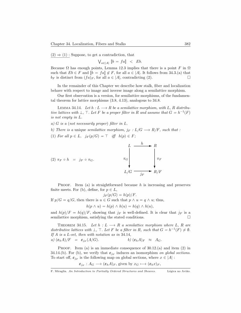
Chapter 34. Localization, Fibers and Stalks 382
(2) ⇒ (1) : Suppose, to get a contradiction, that∨a∈|A| [[b = fa]] < Eb.
Because Ω has enough points, Lemma 12.3 implies that there is a point F in Ωsuch that Eb ∈ F and [[b = fa]] 6∈ F , for all a ∈ |A|. It follows from 34.3.(a) thatbF is distinct from (fa)F , for all a ∈ |A|, contradicting (2).
In the remainder of this Chapter we describe how stalk, fiber and localizationbehave with respect to image and inverse image along a semilattice morphism.
Our first observation is a version, for semilattice morphisms, of the fundamen-tal theorem for lattice morphisms (3.8, 4.13), analogous to 34.8.
Lemma 34.14. Let h : L −→ R be a semilattice morphism, with L, R distribu-tive lattices with ⊥, >. Let F be a proper filter in R and assume that G = h−1(F )is not empty in L.
a) G is a (not necessarily proper) filter in L.
b) There is a unique semilattice morphism, jF : L/G −→ R/F , such that :
(1) For all p ∈ L, jF (p/G) = > iff h(p) ∈ F ;
(2) πF h = jF πG.
L/G
L
?
- R
πG
h
R/F
πF
jF
?-
Proof. Item (a) is straightforward because h is increasing and preservesfinite meets. For (b), define, for p ∈ L,
jF (p/G) = h(p)/F .
If p/G = q/G, then there is u ∈ G such that p ∧ u = q ∧ u; thus,
h(p ∧ u) = h(p) ∧ h(u) = h(q) ∧ h(u),
and h(p)/F = h(q)/F , showing that jF is well-defined. It is clear that jF is asemilattice morphism, satisfying the stated conditions.
Theorem 34.15. Let h : L −→ R a semilattice morphism where L, R aredistributive lattices with ⊥, >. Let F be a filter in R, such that G = h−1(F ) 6= ∅.If A is a L-set, then with notation as in 34.14,
a) (εhA)/F = εjF (A/G). b) (εhA)F ≈ AG.
Proof. Item (a) is an immediate consequence of 30.12.(a) and item (2) in34.14.(b). For (b), we verify that εjF induces an isomorphism on global sections.To start off, εjF is the following map on global sections, where x ∈ |A| :
εjF : AG −→ (εhA)F , given by xG 7−→ (εhx)F ,
F. Miraglia. An Introduction to Partially Ordered Structures and Sheaves. Logica no Aviao.
Chapter 34. Localization, Fibers and Stalks 383
that is, it sends the germ of x at G, to the germ of εhx at F . Clearly, εjF issurjective. If x, y ∈ |A| are such that (εhx)F = (εhy)F in the fiber of εhA at F ,34.3.(b) entails
h(Ex) = Eεhx ∈ F ; h(Ey) = Eεhy ∈ F ;
h([[x = y]]) = [[εhx = εhy]] ∈ F .These relations imply Ex, Ey, [[x = y]] ∈ G, i.e., xG = yG, showing that εjF isalso injective and completing the proof.
Remark 34.16. If G in 34.15 is empty, then the fiber of εhA at F is alsoempty, for there is no x ∈ |A| for which Eεhx ∈ F . If the fiber at the empty setis defined to be empty, then item (b) will hold in a trivial way. 2
All the classical relations between fibers and stalks along change of base areconsequences of 34.15. We register a sample of these as illustration.
Corollary 34.17. a) Let L, R be frames and h : L −→ R be a frame-morphism. If F is a point in R, then
(1) G = h−1(F ) is a point in L.
(2) For all L-sets A, (cA)G ≈ AG ≈ (εhA)F ≈ (chA)F .
b) If f : X −→ Y is a continuous map of topological spaces and B is a presheafover Y , then, for all x ∈ X, (f∗B)x ≈ Bfx. 2
Corollary 34.18. Let h : L −→ R be a semilattice morphism of distributivelattices with ⊥, >. Assume that h has a right adjoint g and let K be a proper filterin L.
a) If B is a R-presheaf and K is a proper filter in L, then
(ihB)K ≈ (εgB)K ≈ B(g−1K).
b) If h is surjective, F is a proper filter in R and A is a L-presheaf, then
(ihεhA)(h−1F ) ≈ (εhA)F .
c) If h is injective, F is a proper filter in L and B is a R-presheaf, then
(chihB)(g−1F ) ≈ (cgB)F ≈ (εgB)F .
Proof. a) Since gh ≥ IdL, it follows that
u ∈ K ⇒ ghu ∈ K.
Hence, g−1(K) 6= ∅ and 34.15 entails (εgB)K ≈ Bg−1K . The other isomorphismis a consequence of the fact that εgB is restriction dense in ihB (33.9.(b)) and34.4.(d).
b) Since h g = IdR, we have g−1(h−1(F )) = F . Hence, item (a) applies to yield
(ihεhA)h−1F ≈ (εhA)(g−1h−1F ) = (εhA)F ,
as needed. Item (c) is analogous and left to the reader.
F. Miraglia. An Introduction to Partially Ordered Structures and Sheaves. Logica no Aviao.

Chapter 34. Localization, Fibers and Stalks 384
Exercises
34.19. Let A be a commutative ring with identity and cA be the structuresheaf of A over Spec(A), as in 27.21.
a) For P ∈ Spec(A), let NP = Za : a 6∈ P be the set of basic open neighborhoodsof P in Spec(A). Then, with Sa = an : n ≥ 0,
P = 〈AS−1a ; ρba : Za ⊆ Zb in NP 〉
is an inductive system of rings over the up-directed poset NopP , with lim→ P = AP ,
the localization of A at P (9.41).
b) Determine the stalk of cA at the point P ∈ Spec(A).
c) If A is a regular ring (19.19), then for all P ∈ Spec(A), AP is (isomorphic to)the residue field A/P . 2
34.20. Let A be an extensional presheaf over the topological space X. Showthat there is a geometrical sheaf over X, cA, together with a presheaf morphism,c : A −→ cA, which satisfies the conditions in Theorem 27.9 10. 2
34.21. Let Ω be a frame with enough points (12.6).
a) If A ⊆ B are sheaves over Ω, the following are equivalent :
(1) A = B; (2) For all points F in Ω, AF = BF .
b) Let f : A −→ B be a morphism of sheaves over Ω. The following are equivalent :
(1) f is an isomorphism; (2) For all points F in Ω, fF is a bijection. 2
34.22. State and prove a result similar to 34.18, with semilattice morphismonto 2 (34.7) in place of filters. 2
34.23. Let R be a commutative ring with identity and let R be the structuresheaf of R over X = Spec(R) as in 27.21 and 27.22. Let ι : Xc −→ X be theidentity map, where Xc is Spec(R) endowed with the constructible topology (as inTheorem 20.10). Describe the inverse image ofR along ι, establishing, in particularthat for all P ∈ X, the stalk of ι∗R at P is the localization RP . 2
10This is the classical version of completion.
F. Miraglia. An Introduction to Partially Ordered Structures and Sheaves. Logica no Aviao.
CHAPTER 35
Regularization Functors
In this Chapter it will be shown that if k : L −→ R is a semilattice morphismwith a right adjoint, there is a functor
kr : Lset −→ Lset,
such that for all L-sets A, with a compatible structure of presheaf (26.6), krA isnaturally isomorphic to ikεkA. We shall assume the reader familiar with the imageand inverse image constructions, discussed in the preceding Chapters.
35.1. The L-set krA. Assume that k : L −→ R has a right adjoint, that is,there is a semilattice morphism, g : R −→ L, such that
[adj] For all 〈 p, r 〉 ∈ L × R, kp ≤ r iff p ≤ gr.
As usual in this situation (7.8), we have
(*)
(i) ∀ 〈 p, r 〉 ∈ L × R, p ≤ gk(p) and kg(r) ≤ r;
(ii) kgk = k and gkg = g.
Let
|A| = 〈x, p 〉 ∈ |A| × H : Ex ≤ p and k(Ex) = k(p).For 〈x, p 〉, 〈 y, q 〉 ∈ |A| set 1
(**) [[〈x, p 〉 = 〈 y, q 〉]]r =def p ∧ q ∧ gk([[x = y]])).
It is straightforward that (**) defines an equality in |A|, with which it becomes aL-set A 2. Furthermore, the first relation in (∗).(i) above entails
Er〈x, p 〉 =def [[〈x, p 〉 = 〈x, p 〉]]r = p ∧ gk(Ex) = p ∧ gk(p)
= p.
In general, A is not extensional. In fact, we have
Fact 35.2. For 〈x, p 〉, 〈 y, q 〉 ∈ |A|, the following are equivalent
(1) Er〈x, p 〉 = Er〈 y, q 〉 = [[〈x, p 〉 = 〈 y, q 〉]]r;(2) p = q and k(Ex) = k(Ey) = k([[x = y]]).
Proof. If (1) holds, then, p= q and p≤ gk([[x = y]]). Since k(Ex) = p = k(Ey),the equations in (∗).(ii) imply k(Ex) = k(Ey) ≤ k([[x = y]]), and (2) followsimmediately. Conversely, if (2) holds, then applying g to all terms yields
1Of course, [[x = y]] is the equality in A.2Clearly, |A| = |skA| (28.4), and so (**) defines another equality in the same domain. However,we have preferred to maintain notations distinct.
385

Chapter 35. Regularization Functors 386
gk(Ex) = gk(Ey) = gk([[x = y]]),
and the first inequality in (∗).(i) entails p = q = p ∧ q ∧ gk([[x = y]]), whichis equivalent to (1). 2
It is clear that (2) defines an equivalence relation on |A|, and that the domainof the extensionalization (30.8) of A is the set of these equivalence classes. Let
krA = εA
be the extensionalization of A. We shall use the same name for an elementof |A| and for its equivalence class in |krA|. Hence, for 〈x, p 〉, 〈 y, q 〉 ∈ |krA|
〈x, p 〉 = 〈 y, q 〉 iff p = q and k(Ex) = k(Ey) = k([[x = y]]);
[[〈x, p 〉 = 〈 y, q 〉]]r = p ∧ q ∧ gk([[x = y]]);
Er〈x, p 〉 = p.
Since Er〈 a,Ea 〉 = Ea and
[[〈 a,Ea 〉 = 〈 b, Eb 〉]]r = Ea ∧ Eb ∧ gk([[a = b]]) ≥ [[a = b]],
krA comes equipped with a L-set morphism, kr : A −→ krA, a 7−→ 〈 a,Ea 〉.
A morphism f : A −→ B of L-sets, induces a morphism
krf : krA −→ krB, 〈x, p 〉 7−→ 〈 fx, p 〉.
Indeed, clearly krf preserves extent. For 〈x, p 〉, 〈 y, q 〉 ∈ |krA|, since g k isincreasing, it follows that
[[〈 fx, p 〉 = 〈 fy, q 〉]]r = p ∧ q ∧ gk([[fx = fy]])
≥ p ∧ q ∧ gk([[x = y]]) = [[〈x, p 〉 = 〈 y, q 〉]]r,
as needed. It is straightforward that
kr(IdA) = IdkrA and kr(f g) = krf krg. 2
Definition 35.3. Let k : L −→ R be a semilattice morphism, with a rightadjoint g. The construction in 35.1 is the regularization functor associated tok, kr : Lset −→ Lset.
We now prove that
∗ The image of krA along k is isomorphic to εkA (35.4.(a));
∗ In case A has a presheaf structure compatible with its equality, krA is naturallyisomorphic to ikεkA (35.4.(c)). For this, it is enough to show that krA has thecorresponding universal property (33.3.(b)).
Theorem 35.4. Let k : L −→ R be a semilattice morphism with a rightadjoint g. Let A be a L-set.
a) The map jA : |krA| −→ |εkA|, given by 〈x, p 〉 7→ εkx is surjective and deter-mines a morphism in SLset, 〈 jA, k 〉 : krA −→ εkA, making the triangle below-leftcommutative :
F. Miraglia. An Introduction to Partially Ordered Structures and Sheaves. Logica no Aviao.
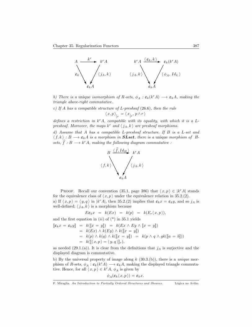
Chapter 35. Regularization Functors 387
A - krA
εk 〈 jA, k 〉
εkA
kr
AAAAAU
krA - εk(krA)
〈 jA, k 〉 〈φA, IdL 〉
εkA
〈 εk, k 〉
AAAAAU
b) There is a unique isomorphism of R-sets, φA : εk(krA) −→ εkA, making thetriangle above-right commutative.
c) If A has a compatible structure of L-presheaf (26.6), then the rule
〈x, p 〉|r = 〈x|r, p∧ r 〉
defines a restriction in krA, compatible with its equality, with which it is a L-presheaf. Moreover, the maps kr and 〈 jA, k 〉 are presheaf morphisms.
d) Assume that A has a compatible L-presheaf structure. If B is a L-set and〈 f, k 〉 : B −→ εkA is a morphism in SLset, there is a unique morphism of H-
sets, f : B −→ krA, making the following diagram commutative :
B - krA
〈 f, k 〉 〈 jA, k 〉
εkA
〈 f , IdH 〉
AAAAAU
Proof. Recall our convention (35.1, page 386) that 〈x, p 〉 ∈ |krA| standsfor the equivalence class of 〈x, p 〉 under the equivalence relation in 35.2.(2).
a) If 〈x, p 〉 = 〈 y, q 〉 in |krA|, then 35.2.(2) implies that εkx = εky, and so jA iswell-defined; 〈 jA, k 〉 is a morphism because
Eεkx = k(Ex) = k(p) = k(Er〈x, p 〉),and the first equation in (ii) of (*) in 35.1 yields
[[εkx = εky]] = k([[x = y]]) = k(Ex ∧ Ey ∧ [[x = y]])
= k(Ex) ∧ k(Ey) ∧ k([[x = y]])
= k(p) ∧ k(q) ∧ k([[x = y]]) = k(p ∧ q ∧ gk([[a = b]]))
= k([[〈x, p 〉 = 〈 y, q 〉]]r),as needed (29.1.(a)). It is clear from the definitions that jA is surjective and thedisplayed diagram is commutative.
b) By the universal property of image along k (30.3.(b)), there is a unique mor-phism of R-sets, φA : εk(krA) −→ εkA, making the displayed triangle commuta-tive. Hence, for all 〈x, p 〉 ∈ krA, φA is given by
φA(εk〈x, p 〉) = εkx.
F. Miraglia. An Introduction to Partially Ordered Structures and Sheaves. Logica no Aviao.
Chapter 35. Regularization Functors 388
Since jA is surjective, φA is also surjective. To show that it is injective, we use25.21, recalling the equations in (∗).(ii) in 35.1, to obtain
[[φA(εk〈x, p 〉) = φA(εk〈 y, q 〉)]] = [[εkx = εky]] = k([[x = y]])
= k(Ex ∧ Ey ∧ [[x = y]]) = k(p ∧ q ∧ [[x = y]])
= k(p ∧ q ∧ gk([[x = y]])) = k([[〈x, p 〉 = 〈 y, q 〉]]r)= [[εk〈x, p 〉 = εk〈 y, q 〉]],
completing the proof of (b). Item (c) is straightforward.
c) Fix a morphism 〈 f, k 〉 : B −→ εkA; for b ∈ |B|, let xb in |A| be such thatfb = εkx
b. Since 〈 f, k 〉 is a morphism, for all c, b ∈ |B|, we have
(F)
(i) Efb = k(Eb) = k(Exb);
(ii) k([[b = c]]) ≤ [[fb = fc]] = [[εkxb = εkx
c]]
= k([[xb = xc]]).
Applying g to inequality (ii) in (F) yields, by (∗).(i) in 35.1,
(G) [[b = c]] ≤ gk([[b = c]]) ≤ gk([[xb = xc]]).
With these preliminaries, note that (i) in (F) entails
Exb ∧ Eb = E(xb|Eb) ≤ Eb and k(Exb ∧ Eb) = k(Eb).
Hence, 〈xb|Eb, Eb 〉 ∈ |krA|. Define f b = 〈xb|Eb, Eb 〉.
We have, Efb = Er〈xb|Eb, Eb 〉 = Eb, showing that f verifies [mor 1] in 25.10.
If b, c ∈ |B|, (G) yields [[f b = f c]] = [[〈xb|Eb, Eb 〉 = 〈xc|Ec, Ec 〉]]
= Eb ∧ Ec ∧ gk([[xb|Eb = xc|Ec]])
= Eb ∧ Ec ∧ gk(Eb ∧ Ec ∧ [[xb = xc]])
= Eb ∧ Ec ∧ gk([[xb = xc]])
≥ Eb ∧ Ec ∧ [[b = c]] = [[b = c]],
verifying [mor 2] in 25.10. For b ∈ |B|, (i) in (F) above yields
jA(〈xb|Eb, Eb 〉) = εk(xb|Eb) = (εkxb)|k(Ep)
= fb|h(Ep)= fb,
verifying the commutativity of the displayed triangle. It remains to check unique-ness. Let β : B −→ krA be a morphism of L-sets, for which the triangle in thestatement is commutative. For b ∈ |B|, write βb = 〈 y, q 〉. Clearly, q = Eb ≥ Ey.Since, jA(〈 y, q 〉) = εky, we conclude that εky = εkx
b. Consequently,
k(Ey) = k(Exb) = k(Eb) = k([[xb = y]]).
These equations and (∗).(i) in 35.1 furnish
[[〈xb|Eb, Eb 〉 = 〈 y, Eb 〉]] = Eb ∧ gk([[xb|Eb = y]]) = Eb ∧ gk(Eb ∧ [[xb = y]])
= Eb ∧ gk([[xb = y]]) = Eb
and the extensionality of krA guarantees that βb = f b, as needed.
From item (d) in Theorem 35.4 we get
F. Miraglia. An Introduction to Partially Ordered Structures and Sheaves. Logica no Aviao.

Chapter 35. Regularization Functors 389
Corollary 35.5. Let k : L −→ R be a semilattice morphism with a rightadjoint. If A is has compatible structures of L-set and L-presheaf, then krA isnaturally isomorphic to ikεkA. 2
Lemma 35.6. If k : L −→ R is a semilattice morphism with a right adjoint,the functor kr : Lset −→ Lset preserves all finite products.
Proof. Let 1 be the final object in Lset (25.5). From the definition of kr,it follows that |kr1| = 〈x, p 〉 ∈ L × L : x ≤ p and kx = kp, where 〈x, p 〉is identified with 〈 y, p 〉 if k(x) = k(y) = k(x ∧ y). Hence, 〈x, p 〉 = 〈 p, p 〉 in kr1and so kr1 = 1. If A1, . . . , An are L-sets, the map
〈x, p 〉 ∈ |kr(∏ni=1 Aj)| 7−→ 〈 〈x1, p 〉, . . . , 〈xn, p 〉 〉 ∈ |
∏ni=1 k
rAj |is easily seen to be an isomorphism.
35.7. The regularization associated to double negation. There is aspecial case of regularization 3 that is important in applications to logic : whenH is a Heyting algebra and the semilattice morphism k is the canonical quotientmap πD : H −→ H/D, where D is the filter of dense elements in H (6.19, 6.20,10.5). Note that even if H is not complete, πD has a right adjoint,
g(p/D) = ¬¬ p.In this case :
[r 1] : Write rA for πrDA. Thus,
|rA| = 〈x, p 〉 ∈ |A| × H : Ex ≤ p and ¬¬Ex = ¬¬ p,with the convention that
〈x, p 〉 = 〈 y, q 〉 iff p = q and ¬¬Ex = ¬¬Ey = ¬¬ [[x = y]].
Moreover, equality in rA is given by
[[〈x, p 〉 = 〈 y, q 〉]]r = p ∧ q ∧ ¬¬ [[x = y]].
[r 2] : Write r : A −→ rA for the morphism x 7−→ rx =def 〈x,Ex 〉;[r 3] : If f : A −→ B is a H-set morphism, rf : rA −→ rB is given by
rf(〈x, p 〉) = 〈 fx, p 〉. 2
The results in this Chapter, together with 34.18, yield
Corollary 35.8. Let H be a Heyting algebra and D the filter of denseelements in H. Let A have compatible structures of H-set and H-presheaf.
a) The functor r : Hset −→ Hset preserves all finite products.
b) rA ≈ iπd(A/D), A/D = (rA)/D and (rA)D = AD. 4
c) If F is a prime filter in the BA H/D, then (A/D)F ≈ rA(π−1D F ), i.e. the
stalk of A/D at F coincides with the stalk of rA at the ultrafilter π−1D (F ) of H. 2
When H is a frame, we have,
3Actually, the origin for the terminology.4AD is the fiber of A at D, as in 34.6.
F. Miraglia. An Introduction to Partially Ordered Structures and Sheaves. Logica no Aviao.
Chapter 35. Regularization Functors 390
Proposition 35.9. If H is a frame and A is a sheaf over H, then rA is asheaf over H and A/D is a sheaf over H/D.
Proof. There are two ways to establish our result :
∗ Show that rA is a sheaf and conclude by 33.9.(e).(2) and 29.6;
∗ Show that A/D is a sheaf and obtain that rA is a sheaf from 33.3.(c).
The basic techniques are similar, and we take the first route.
Let 〈xi, pi 〉 : i ∈ I be a compatible family in |rA|. Thus, ∀ i, j ∈ I,
(A) [[xi = xj ]] ≤ Exi ∧ Exj ≤ pi ∧ pj ≤ ¬¬ [[xi = xj ]].
By 8.25, there is a pairwise disjoint family qi : i ∈ I, such that
(B) ∀ i ∈ I, qi ≤ Exi and∨i∈I Exi ≤ ¬¬
∨i∈I qi.
Let S = (xi)|qi : i ∈ I; since the qi are pairwise disjoint, S is compatible
in A. Let x ∈ |A| be the gluing of S. Hence,
(C)
(i) Ex =
∨i∈I qi;
(ii) qi = [[x = (xi)|qi ]] = qi ∧ [[x = xi]], ∀ i ∈ I.
Thus, Ex ≤ p =def
∨i∈I pi; additionally, Lemma 8.16.(h), ¬¬Exi = ¬¬ pi
and (B) yield
¬¬Ex = ¬¬∨i∈I qi = ¬¬
∨i∈I Exi = ¬¬
∨i∈I ¬¬Exi
= ¬¬∨i∈I ¬¬ pi = ¬¬
∨i∈I pi = ¬¬ p,
and 〈x, p 〉 ∈ |rA|. Then, 〈x, p 〉 is the gluing of the original family in rA; clearly,it has the appropriate extent.
Fact. For all i ∈ I, [[x = xi]] is dense in pi.
Proof. Let α = j ∈ I : Exi ∧ qj 6= ⊥; from (B) comes
(D) ¬¬Exi = ¬¬Exi ∧ ¬¬∨j∈I qj = ¬¬ (Exi ∧
∨j∈I qj)
= ¬¬∨j∈A Exi ∧ qj .
Consequently, for j ∈ α, (A) and (C).(ii) entail
¬¬ [[x = xi]] ≥ ¬¬(
[[x = (xj)|qj ]] ∧ [[(xj)|qj = xi]])
= ¬¬ (qj ∧ [[xi = xj ]]) = ¬¬ qj ∧ ¬¬ [[x = xi]]
= ¬¬ qj ∧ ¬¬ (Exi ∧ Exj) = ¬¬ (qj ∧ Exi ∧ Exj)= ¬¬ (qj ∧ Exi).
Whence, taking joins with respect to j ∈ α, (D) and (A) yield
¬¬ [[x = xi]] ≥ ¬¬∨j∈A ¬¬ (qj ∧ Exi) = ¬¬
∨j∈A Exi ∧ qj
= ¬¬Exi = ¬¬ pi,as claimed.
With the Fact, we then obtain
[[〈x, p 〉 = 〈xi, pi 〉]]r = p ∧ pi ∧ ¬¬ [[x = xi]] = pi ∧ ¬¬ [[x = xi]]
= pi = E〈xi, pi 〉,and 〈x, p 〉 is the gluing of the 〈xi, pi 〉, as desired.
F. Miraglia. An Introduction to Partially Ordered Structures and Sheaves. Logica no Aviao.

Part 7
Characteristic Maps

Introduction
Characteristic maps are a means to construct an algebra of relations in thecategories Ωset and pSh(Ω). The attentive reader will realize that many of ourdefinitions and results are valid for general L-sets and L-presheaves. However, com-pleteness of the base algebra guarantees that certain (possibly infinite) joins andmeets, associated to quantification, exist in the algebra of characteristic functionsand for this reason we concentrate on objects whose base algebra is a frame. Theoriginal idea for this development appeared in [50]; [52] describes how analogousmethods may be applied to deal with subobjects in presheaves over idempotentquantales.
Although our main interest is establishing the basic structures needed to de-velop Model Theory in the category of Ω-presheaves, we shall also work with Ω-setsin order to guarantee a certain generality to our constructions, as well as to in-dicate the difficulties that arise when the domain of a first-order structure is nota presheaf. Since in first-order languages relation and function symbols, althoughfinitary, might depend on arbitrarily large finite sets of variables, it seems appro-priate to deal with arbitrary powers of a Ω-object. Moreover, if A and B are thedomains of first-order structures, it is important to describe how relations in Atransfer to B along a morphism. In this respect, inverse image is more importantthan direct image. Indeed, recall that if M , N are first-order structures, a map f: M −→ N is a L-morphism if for each n-ary relation R in L and a ∈ Mn
M |= R[a] ⇒ N |= R[fa].
This may be rephrased in terms of characteristic maps as RM ≤ f∗RN , whereR(·) is the characteristic map of the interpretation of R. In a similar vein, f is aL-monic if RM = f∗RN and an elementary embedding if a corresponding relationholds for all formulas.
The family of all characteristic maps on a Ω-set, as well as the collection of suchmaps that depend on a fixed subset of the index set, constitute frames. However,the family of all characteristic maps that depend on some finite subset of the indexset does not have a natural structure of a frame. Nevertheless, it can be described asan inductive limit of an inductive system of frames of characteristic maps on finitepowers of the base domain, together with open injections. Consequently, we haveincluded material on the graded frame that arises by considering characteristicmaps on finite powers of a Ω-set.
Even if we had adopted a completely finitistic approach, to establish the sound-ness of the Heyting Predicate Calculus for presheaves of structures over a frame,
392

Introduction 393
requires that characteristic maps defined on distinct finite powers, having as expo-nents subsets α, β of the natural numbers, be considered as characteristic maps onthe power whose exponent is the union α ∪ β. This corresponds to a well-knownidentification : a formula in the variables indexed by α, is considered as formulain the variables indexed by α ∪ β. This, in turn, originates with the fact that forn ≤ m, a subset of An can be identified with a subset of Am, via inverse image bythe projection that forgets coordinates outside n. This identification correspondsprecisely to taking, as interpretations of formulas in n free variables, the inductivelimit of its interpretations in Am, where n ≤ m.
Experience has shown that it is easier to handle the values of formulas ifone does have to worry about the extent of the arguments. Hence, characteristicmaps will be defined on a power of the domain of the base object (37.1). For Ω-presheaves – but not for Ω-sets –, this is equivalent to characteristic maps definedin the domain of the corresponding power of the base object (38.7). However, thegenerality and practical merits of the definition we have adopted justify the effortin developing its properties.
Unless otherwise explicitly stated, all objects are extensional and allsemilattices have ⊥ and >.
F. Miraglia. An Introduction to Partially Ordered Structures and Sheaves. Logica no Aviao.
CHAPTER 36
Closure
This Chapter discusses results of section 24.2 in the categories Ωset andpSh(Ω). The proofs for Ω-presheaves are so similar that we shall frequently omitthem. The notion of denseness is defined in 25.32.
Definition 36.1. Let A be a Ω-set and S ⊆ |A|. The closure of S in A is
S = x ∈ |A| : Ex =∨s∈S [[x = s]].
Clearly, S ⊆ S. We say that S is closed in A if S = S. Write P>(A) for thefamily of closed subsets of A. If the domain in which the closure operation is being
performed has to be displayed, we write SA
for S. The superscript will always beomitted whenever clear from context.
Remark 36.2. Recall our convention (25.1) that an Ω-set A has a uniquesection of extent ⊥, written ∗. For all S ⊆ |A|
⊥ = E∗ =∨s∈S [[∗ = s]],
and so ∗ ∈ S; ∗ is clearly closed and so it is the least closed subset of A. 2
Recall (25.3) that if A is a Ω-set, S ⊆ |A| and p ∈ Ω,
∗ The restriction of S to p, S|p, is the sub-Ω-set of A whose domain is
|S|p| = x ∈ |A| : Ex ≤ p;
∗ The extent of S is ES =∨x∈S Ex.
Lemma 36.3. Let A be a Ω-set and S, T ⊆ |A|.a) ES = ES.
b) T ⊆ S iff S is dense in T .
c) If S ⊆ T , then S = T iff S is dense in T .
d) The closure operation is increasing, inflationary and idempotent 1.
e) The intersection of any family of closed subsets of is closed.
f) If S is closed in A, then S ∩ T is closed in T .
g) If S is closed and T ⊆ S is a compatible set in A, whose gluing t exists in A,then t ∈ S.
1That is, S ⊆ T ⇒ S ⊆ T , S ⊆ S and S = S.
394
Chapter 36. Closure 395
Proof. Items (a), (b), (c) and (f) are clear, as is the fact that closure isincreasing and inflationary in (d). For idempotency, we have
S dense in S, S dense in S,
and the conclusion follows from (c) and the transitivity of denseness (25.33.(a)).For (e), let Si, i ∈ I, be closed subsets of |A|, and set S =
⋂i∈I Si. By (c),
S ⊆ Si = Si, for all i ∈ I,
and S ⊆ S, i.e., S is closed in A. For (g), let T ⊆ S be compatible in A, withgluing t. Then, [glu p] in 25.30, with p = >, yields
Et =∨u∈T [[t = u]] ≤
∨s∈S [[t = s]],
and so t ∈ S, as asserted.
For Ω-presheaves, closure has the following additional properties :
Lemma 36.4. Let A be a Ω-presheaf, S, T be subpresheaves of A and p ∈ Ω.
a) The following conditions are equivalent :
(1) S = S;
(2) ∀ t ∈ |A|, ∀ α ⊆ Ω,∨α = Et and t|q ∈ |S| ⇒ t ∈ |S|.
b) S ∩ T = S ∩ T .
c) All closed subsets of |A| are subpresheaves of A.
d) Closure commutes with restriction, i.e., (S|p) = S|p.
e) If A is a sheaf, then S is closed in A iff S is a subsheaf of A.
Proof. Item (a) is straightforward. For (b), first note that 36.3.(b) entailsS ∩ T ⊆ S ∩ T . Let x ∈ S ∩ T ; then
(I) Et =∨s∈S [[x = s]] =
∨t∈T [[x = t]].
Let D = s|([[x=s]]∧[[x=t]])∈ |A| : s ∈ S, t ∈ T. Note that for all 〈 s, t 〉 ∈ S × T ,
(II) s|[[x=s]]∧[[x=t]]= x|[[x=s]]∧[[x=t]]
= t|[[x=s]]∧[[x=t]].
Since S, T are subpresheaves of A, (II) entails D ⊆ (S ∩ T ). But then (I) yields∨d∈D [[x = d]] =
∨〈s,t〉∈S×T [[x = s|[[x=s]]∧[[x=t]]
]]
=∨〈s,t〉∈S×T [[x = s]] ∧ [[x = t]]
=∨s∈S [[x = s]] ∧
∨t∈T [[x = t]] = Et
showing that x ∈ S ∩ T .
c) It is enough to show that a closed subset is closed under restriction. Let C bea closed subset of A, x ∈ C and p ∈ Ω. Then∨
c∈C [[x|p = c]] ≤ [[x|p = x]] = p ∧ Ex = Ex|p,
F. Miraglia An Introduction to Partially Ordered Structures and Sheavesc©2005 Polimetrica International Scientific Publisher Monza/Italy

Chapter 36. Closure 396
and so x|p ∈ S = S, as desired. For (d), since restriction to p is obviously increas-
ing, it suffices to check that |S|p| ⊆ |(S|p)|. If x ∈ |S|p|, then, because S is a
subpresheaf, and Ex ≤ p, we obtain
Ex =∨s∈|S| [[x = s]] =
∨s∈|S| p ∧ [[x = s]] =
∨s∈|S| [[x = s|p]]
≤∨d∈|S|p| [[x = d]],
and x ∈ |(S|p)|, as needed. The proof of (e) is analogous to that of 24.13.
Observe that
∗ If A is a Ω-presheaf, 36.4.(b) entails that P>(A) is the family of closed sub-presheaves of A;
∗ If A is a Ω-sheaf, 36.4.(d) implies that P>(A) is the family of subsheaves of A.
Corollary 36.5. If A is a Ω-set or a Ω-presheaf, 〈P>(A), ⊆〉 is a completelattice, with meets given by intersection.
Proof. Follows from 36.3.(d), 36.4.(b) and the fact that (set-theoretic) in-tersection of subpresheaves is a subpresheaf.
If Si, i ∈ I, are closed subsets of a Ω-set or a Ω-presheaf A, then 2
(∨
)∨i∈I Si =
⋃i∈I Si
is the join of the Si in the complete lattice P>(A).
Remark 36.6. If A is a Ω-set, P>(A) is almost a Ω-presheaf. By Exercise36.14, closure is preserved by restriction. It is then straightforward that the maps
S ∈ P>(A) 7−→ ES ∈ Ω
〈S, p 〉 ∈ P>(A) × Ω 7−→ S|p ∈ P>(A),
satisfy [rest 1] and [rest 3] in Definition 23.1, but, in general, not [rest 2] 3.
However, if A is a Ω-presheaf, then [rest 2] is verified and P>(A) is a Ω-presheaf. In this case, Proposition 26.8 yields, for S, T ∈ P>(A),
[[S = T ]] =∨p ∈ Ω : p ≤ ES ∧ ET and S|p = T|p
=∨p ∈ Ω : p ≤ ES ∧ ET and |S|p| = |T|p|.
The reader is invited to show that, with the presheaf structure defined above,P>(A) is a sheaf over Ω, whenever A is an extensional Ω-presheaf. 2
Example 36.7. Let |A| = a, b, c, ∗ be a set with four elements and letB = ⊥, p, ¬ p, > be the four-element BA. Define, for x, y ∈ |A| − ∗
2By 36.4.(b), in the case of presheaves.3One may have S|p = ∗, with ES = >.
F. Miraglia An Introduction to Partially Ordered Structures and Sheavesc©2005 Polimetrica International Scientific Publisher Monza/Italy
Chapter 36. Closure 397
[[x = y]] = [[y = x]] =
> if x = y;
p if x = a and y = c;
¬ p if x = b and y = c;
⊥ if x = a and y = b,
while [[x = ∗]] = [[∗ = x]] = ⊥. It is straightforward that this defines a equality on|A|, with which it is an extensional B-set. Note that for all x ∈ |A| − ∗, x, ∗is closed in A. Moreover, a, b is dense in A, because
> = Ec = [[c = a]] ∨ [[c = b]] = p ∨ ¬ p.Thus, c, ∗ ∩ (a, ∗ ∨ b, ∗) = c, ∗ ∩ |A| = c, ∗; on the other hand,c, ∗ ∩ a, ∗ = ∗ = c, ∗ ∩ b, ∗. Hence, P>(A) is not distributive andso cannot be a frame. As we shall see shortly, this changes if A is a presheaf. 2
Theorem 36.8. Let A be a Ω-presheaf.
a) P>(A) is a frame, whose meets are (set-theoretic) intersections and whose joinsare given by formula (
∨) on page 396.
b) If B is a dense subpresheaf of A, then the map
T ∈ P>(B) 7−→ TA ∈ P>(A)
is a frame-isomorphism.
c) The map defined in (b) is a frame isomorphism between P>(A) and P>(cA),where cA is the completion of A over Ω (27.9).
Proof. a) By 36.3.(a) and 36.4.(a), the map
? : 2|A| −→ P>(A)
is a nucleus on the cBa 2|A| (13.1). Hence, Theorem 13.2.(d) entails that P>(A) isa frame. Item (a) in Theorem 7.5, together with the proof of 13.2, guarantee thatmeets and joins in P>(A) are as asserted.
b) By 36.3.(d), the displayed map is increasing. Hence, to show that it is anisomorphism, it is enough to check that it is a bijection.
For T , T ′ ∈ P>(B), assume that TA
= T ′A
. By 36.3.(b), T , T ′ are dense ineach other in A and so the same must be true in B. Since they are closed relativeto B, we must have T = T ′, verifying injectivity. If S is a closed subset of A, let Tbe the subpresheaf of B whose domain is (|B| ∩ |S|); T is closed in B (36.3.(f)) and
dense in S, because B is dense in A. Thus, TA
= S, establishing surjectivity.
The next result simplifies computations in non-empty powers of presheaves.
Lemma 36.9. Let A be a Ω-presheaf and I 6= ∅ be a set. For S ⊆ |A|I , set 4
pS = s|Es ∈ AI : s ∈ S.
Then, pS = x ∈ |AI | : Ex =∨s∈S [[x = s]].
4Note that S ⊆ |AI | iff pS = S.
F. Miraglia An Introduction to Partially Ordered Structures and Sheavesc©2005 Polimetrica International Scientific Publisher Monza/Italy
Chapter 36. Closure 398
Proof. Recall that AI has a natural presheaf structure (26.12), compatiblewith its equality, given by (25.12) [[x = y]] =
∧i∈I [[xi = yi]]. For x ∈ |AI |
and s ∈ S, 26.8.(b) yields [[x = s]] = [[x = s|Es]], with s|Es ∈ pS. Hence,∨s∈S [[x = s]] =
∨c∈pS [[x = c]], and the conclusion follows immediately.
Remark 36.10. If A is an extensional Ω-presheaf, define a Ω-presheaf P(A)by the following prescriptions :
∗ |P(A)| = 〈S, p 〉 ∈ (P>(A) × Ω) : ES ≤ p; ∗ E〈S, p 〉 = p;
∗ 〈S, p 〉|q = 〈S|q, p ∧ q 〉.
As was the case for presheaves of sets, discussed in section 24.2 (24.38),
P(A) is a Ω-sheaf, whose set of global sections is P>(A).
Moreover, [[〈S, p 〉 = 〈T, q 〉]] =∨u ≤ p ∧ q : S|u = T|u.
The sheaf P(A) is the sheaf of closed subpresheaves of A. If A is a sheaf,P(A) is the sheaf of subsheaves of A. 2
As for presheaves of sets (24.24, 24.26), we have
Definition 36.11. Let η : A −→ B be a morphism of Ω-sets. If S ⊆ |A|,the image of S by η is
η∗S = ηx : x ∈ S.In particular, Imη is the closure in B of the set-theoretical image of |A| by η. IfT ⊆ |B|, the inverse image of T by η is
η∗T = x ∈ |A| : ηx ∈ T.
Exercises
36.12. Let A be a Ω-set and ∆ = 〈 a, a 〉 : a ∈ |A| be the diagonal ofA2 = A × A.
a) ∆ = 〈x, y 〉 ∈ |A2| : Ex = Ey = [[x = y]].b) A is extensional iff ∆ is a closed subset of A2. 2
36.13. Let 1 be the final object in Ω set (25.5, 26.18). For S ⊆ |1|, as wasthe case in 24.21.(b), S ∈ P>(1) iff S = 1|ES . 2
36.14. Show that restriction takes closed sets to closed sets. 2
36.15. If A is a Ω-presheaf and S, T ⊆ |A|, define 5
S → T = x ∈ |A| : For all p ≤ Ex, x|p ∈ S ⇒ x|p ∈ T.
a) S, T ∈ P>(A) ⇒ S → T ∈ P>(A) and (S → T ) = S → T .
b) S → T is the implication operation in the frame P>(A).
c) If S, T ∈ P>(A), the following are equivalent, for p ≤ ES ∧ ET :
5If S, T are subpresheaves, then S → T = x ∈ |A| : x ∈ |S| ⇒ x ∈ |T |.
F. Miraglia An Introduction to Partially Ordered Structures and Sheavesc©2005 Polimetrica International Scientific Publisher Monza/Italy

Chapter 36. Closure 399
(1) A|p ⊆ (S ↔ T ); (2) S|p = T|p,
where ↔ is the equivalence operation in the frame P>(A). 2
36.16. If A is a Ω-presheaf, P(A) is flabby (31.10.(e)). 2
36.17. Let A be an extensional Ω-presheaf. Write H for the frame P>(A).
a) The map p ∈ Ω 7−→ γ(p) =def A|p ∈ H is an open frame morphism (8.1.(b)).
b) If A = 1, the morphism in (a) is an isomorphism between P>(1) and Ω 6.
c) Let H be the sheaf over H in 27.7 and 25.4. Then, P(A) is the inverse image of
H along the morphism γ in (a) 7. 2
36.18. Let A be an L-set and S ⊆ |A|. The finite closure of S in A is
fcl(S) = s ∈ |A| : ∃ α ⊆f S such that Es =∨a∈α [[s = a]] .
With 36.3 and 36.4 as models, discuss finite closure for L-sets and presheaves. 2
36.19. With 24.25 and 24.27 as parameters, study image and inverse imageby morphisms in Ωset and pSh(Ω), establishing their adjointness. 2
36.20. Let A, B be Ω-presheaves.
a) If S ∈ P>(A) and T ∈ P>(B) then S × T ∈ P>(A × B), where
S × T = 〈 a, b 〉 ∈ |A × B| : a ∈ S and b ∈ T.b) E(S × T ) = ES ∧ ET (ES is the support of S as in 26.1.(c)).
c) The map P>(A) × P>(B) −→ P>(A × B), given by 〈S, T 〉 7−→ S × T , isa frame-morphism, where P>(A) × P>(B) has the product frame structure 8.
d) If S, S′ ∈ P>(A) and T ∈ P>(B), then
(S → S′) × T = (A × T ) ∩(
(S × T ) → (S′ × T ))
;
and, similarly if the first coordinate is kept fixed. Conclude that the mapsP>(A) −→ P>(A × B), S 7−→ S × B
P>(B) −→ P>(A × B), T 7−→ A × T
are open injective frame-morphisms.
e) For 〈S, T 〉, 〈S′, T ′ 〉 ∈ P>(A) × P>(B), the following are equivalent:
(1) S × T = S′ × T ′;
(2)
(a) ES ∧ ET = ES′ ∧ ET ′;(b) S|ES∧ET = S′|ES∧ET and T|ES∧ET = T ′|ES∧ET . 2
36.21. State and prove the generalization of Theorem 24.15 to L-presheaves,assuming that L is a frame wherever necessary. 2
61 is the final object in Ω set; this generalizes 24.21.(c).7No wonder the constructions are so similar.8Note : S × T = π∗A(S) ∩ π∗B(T ), where πA, πB are the natural projections.
F. Miraglia An Introduction to Partially Ordered Structures and Sheavesc©2005 Polimetrica International Scientific Publisher Monza/Italy
CHAPTER 37
Characteristic Maps in Powers of a Ω-set
We shall constantly use the vector notation introduced in 25.13 and 26.11. Thereader should keep in mind the distinction between the domain of a product ofΩ-sets and the domain of their product. If A is a Ω-presheaf and I is a set,
x|Ex is always in |AI | and x|Ex = x iff x ∈ |AI |.
Moreover, if A has a compatible structures of Ω-set and presheaf (26.6), then forall x, y ∈ |A|I and p, q ∈ L,
(Rest) [[x|p = y|q]] = p ∧ q ∧ [[x = y]],
a very useful relation. Exercise 37.21 collects the properties that will be of constantuse.
We begin by defining characteristic maps on powers of a Ω-set. However,most of the results can be readily extended to finite products of Ω-sets or Ω-presheaves, corresponding to relations whose variables range over distinct sorts.Recall (25.15.(a)) that if A is a Ω-set and I 6= ∅ is a set, then∨
a∈|A|I Ea = EA.
Definition 37.1. Let A be a Ω-set and I be a set. A I-characteristic map
on A is a map, |A|I k−→ Ω, such that for x, y ∈ |A|I ,
[ch 1] : k(x) ≤ Ex; [ch 2] : k(x) ∧ [[x = y]] ≤ k(y).
Let KI(A,Ω) be the set of I-characteristic maps on A. Whenever context allows,write KIA for KI(A,Ω). For h ∈ KIA, set
Eh =∨a∈|A|I h(a),
called the extent of h.
If I = n = 1, . . . , n, a I-characteristic map is called a n-characteristicmap on A; write KnA for the set of n-characteristic maps on A.
Remark 37.2. Let A be a Ω-set and I be a set.
a) It is straightforward that [ch 2] in 37.1 is equivalent to
[ch 2′] : k(x) ∧ [[x = y]] = k(y) ∧ [[x = y]],
or yet, using the equivalence in the frame Ω (6.9), [ch 2] and [ch 2′] can be written
[ch 2′′] : [[x = y]] ≤ k(x) ↔ k(y).
400

Chapter 37. Characteristic Maps in Powers of a Ω-set 401
b) If D is a sub-Ω-set of A and k ∈ KIA, write k|D for the restriction of k to |D|I ,called the restriction of k to D. Hence, for d ∈ |D|I , k|D(d) = k(d). Clearly,
k|D is I-characteristic map on D.
c) If h ∈ KIA, it follows from 25.15.(a) and [ch 1] in 37.1 that
Eh =∨a∈|A|I Ea = EA.
Hence, KIA could be defined as the set of maps h : |A|I −→ EA, satisfying [ch 1]and [ch 2] in 37.1. In our setting, the distinction between the definitions is slight,except when treating K∅A, discussed in 37.3, below.
These observations will be of constant use, frequently without explicit reference. 2
Remark 37.3. If I = ∅, a I-characteristic map k : |A|0 −→ Ω is a func-tion from ∗ to Ω. Hence, the statement of 37.1 implies that K∅A is in bijectivecorrespondence with Ω. However, taking 37.2.(c) into account, we shall instead
(!) Identify K∅A with the frame (EA)←.
We shall also write K0A for K∅A.
Convention (!) is adopted to prevent many of our central results to be falsifiedfor trivial reasons. If characteristic maps on A are taken to have codomain EA,which, as noted in 37.2.(c), is equivalent to 37.1, then (!) is immediately forth-coming. On the other hand, one would have to constantly take into account thecodomain of characteristic maps, burdening arguments unnecessarily. A structuralreason for (!) will emerge in Chapter 40 of this Part (see 40.4).
As an additional argument for keeping 37.1, note that if I is finite, it can bestated verbatim for a L-set, where L is any semilattice. 2
The set of I-characteristic maps, KIA, inherits the structure that is present inΩ. Care must be exercised in handling implication and negation. We summarizethe pertinent results, omitting proofs, in
Proposition 37.4. Let A be a L-set and I be a set.
a) There is a partial order on KIA, given by
h ≤ k iff ∀ x ∈ |A|I , h(x) ≤ k(x).
In this partial order, the maps ⊥⊥⊥I and >>>I 1 are the bottom and top of KIA,respectively.
b) If p ∈ L and k ∈ KIA, then p ∧ k ∈ KIA, where for all x ∈ |A|I
(p ∧ k)(x) = p ∧ k(x).
c) If L is a lattice, KIA is a lattice, with meets and joins computed pointwise, i.e.,(∧λ∈Λ hλ
)(x) =
∧λ∈Λ h(x) and
(∨λ∈Λ hλ
)(x) =
∨λ∈Λ hλ(x),
are the meet and join of the hλ in the partial order of (a). Moreover, if L iscomplete or a frame, the same is true of KIA.
d) If L is a HA, KIA is a HA in which implication and negation are given by
1In items (b) and (c) of 37.22.
F. Miraglia. An Introduction to Partially Ordered Structures and Sheaves. Logica no Aviao.

Chapter 37. Characteristic Maps in Powers of a Ω-set 402(h → k)(x) = Ex ∧ (h(x) → k(x));
(¬h)(x) = Ex ∧ ¬h(x),
where → and ¬ in the right-hand side of these formulas are implication and nega-tion in L.
e) If L is a BA, then, with the operations described above, KIA is a Boolean algebra,which is complete whenever the same is true of L.
f) Let SI be the set of permutations of I, that is, the set of bijective maps fromI to I. If σ ∈ SI and x ∈ |A|I , let xσ ∈ |A|I be given by xσi = xσ(i). For
h ∈ KIA, define hσ : |A|I −→ Ω by hσ(x) = h(xσ). Then
(1) hσ ∈ KIA; (2) The map h 7→ hσ is an automorphism of KIA. 2
Example 37.5. Recall (25.5) that 1 is the final object in the category Ωset,where |1| = Ω and [[p = q]] = p ∧ q.
Fact 37.6. Let p ∈ Ω.
a) If k ∈ K11|p, then for all q ∈ |1|p|, k(q) = k(p) ∧ q.b) The map k ∈ K11|p 7−→ k(p) ∈ p← is an isomorphism.
Proof. Keep in mind that |1|p| = p← and that if q ∈ |1|p|,Eq = q = p ∧ q = [[p = q]].
For k ∈ K11|p and q ∈ |1|p|,
k(q) = k(q) ∧ Eq = k(q) ∧ [[p = q]] = k(p) ∧ [[p = q]] = k(p) ∧ q,establishing (a). Since Ep = p, it is clear that k(p) ≤ p. It is immediate from (a)that the map in (b) is injective. Surjectivity comes from 37.4.(b) : if u ≤ p, thenk = u ∧ >>>1 ∈ K11|p and k(p) = u. 4
If A is a Ω-set, then (!) in 37.3 and Fact 37.6 entail 2
K0A ≈ (EA)← ≈ K11|EA.
From this perspective, if I is any set, there is an isomorphic copy of K0A insideKIA, namely the image of the map
p ≤ EA 7−→ p ∧ >>>I ∈ KIA
i.e., the I-characteristic map on A given by a 7→ p ∧ Ea. To see that this map isinjective, note that if p, q ≤ EA are such that
∀ a ∈ |A|I , p ∧ Ea = q ∧ Eathen taking joins on both sides over a yields p ∧ EA = q ∧ EA, and so p = q. Weshall return to this theme in Chapter 40. 2
Example 37.7. Let f : A −→ B be a morphism of Ω-sets and letI be a set.
Fix ξ = b ∈ |B|I and define
kξ : |A|I −→ Ω, by kξ(a) = [[f(a) = b]].
2One is tempted by the idea that the empty power of A should be 1|EA.
F. Miraglia. An Introduction to Partially Ordered Structures and Sheaves. Logica no Aviao.

Chapter 37. Characteristic Maps in Powers of a Ω-set 403
Then, kξ is a I-characteristic map on A. First note that since f is a morphism,
we have kξ(a) ≤ Efa = Ea, for all a ∈ |A|I . If x ∈ |A|I , [[a = x]] ≤ [[fa = fx]]yields
kξ(a) ∧ [[a = x]] = [[fa = b]] ∧ [[a = x]] ≤ [[fa = b]] ∧ [[fa = fx]]
≤ [[fx = b]] = kξ(x),
verifying [ch 2] in 37.1. By 37.2.(a), for all a, x ∈ |A|I
[[fa = b]] ∧ [[a = x]] = [[fx = b]] ∧ [[a = x]]. (*)
The reader has probably noticed that in case I = 1, we have just shown that
certain singletons are in K1(A). Similarly, one verifies that for a ∈ |A|I ,ka(b) = [[fa = b]]
is a I-characteristic map on B. Moreover, by 37.4.(c),(∨a∈|A| ka
)(b) =
∨a∈|A|I [[fa = b]] (**)
is in KIB, since it is a join of elements in KIB. 2
Our next result describes the basic properties of extension and restriction ofcharacteristic maps; its item (c) is a very important property of characteristic mapson finite powers, guaranteeing that if D is dense in A, a characteristic map on Dhas a unique extension to a characteristic map on A.
Theorem 37.8. Let D ⊆ A be Ω-sets and I be a set.
a) For h ∈ KID, define he : |A|I −→ Ω by
he(a) =∨d∈DI [[a = d]] ∧ h(d).
Then, he ∈ KIA and he|D = h 3.
b) The map k ∈ KIA 7−→ k|D ∈ KID is an open (8.1.(c)) surjection.
c) If I is finite and D is dense in A, then the restriction morphism in (b) is anisomorphism, with inverse h 7→ he.
Proof. a) Clearly, he verifies [ch 1] in 37.1. For a, b ∈ |A|I ,he(a) ∧ [[a = b]] = [[a = b]] ∧
∨d∈DI [[a = d]] ∧ h(d)
=∨d∈DI [[a = b]] ∧ [[a = d]] ∧ h(d)
≤∨d∈DI [[b = d]] ∧ h(d) = he(b),
showing that he ∈ KIA. Now, if t ∈ |D|I , we get
he(t) =∨d∈DI [[t = d]] ∧ h(d) =
∨d∈DI [[t = d]] ∧ h(t)
= h(t) ∧∨d∈DI [[t = d]] = h(t) ∧ Et = h(t),
and (he)|D = h, as desired.
b) By (a), restriction is a surjection from KIA onto KID; it is straightforward thatit preserves all meets and joins, as well as implication, being therefore open.
3Restriction is defined in 37.2.(b).
F. Miraglia. An Introduction to Partially Ordered Structures and Sheaves. Logica no Aviao.
Chapter 37. Characteristic Maps in Powers of a Ω-set 404
c) We may assume that I = n = 1, . . . , n. It is enough to check that h|D = k|Dimplies h= k. SinceD is dense in A, for a ∈ |A|n we have Eaj =
∨dj∈|D| [[aj = dj ]],
1 ≤ j ≤ n. Thus, distributivity of joins over finite meets (8.4) yields
Ea =∧nj=1 Eaj =
∧nj=1
∨dj∈|D| [[aj = dj ]] =
∨d∈Dn [[a = d]].
Hence, h(a) = h(a) ∧ Ea = h(a) ∧∨d∈Dn [[a = d]]
=∨d∈Dn h(a) ∧ [[a = d]] =
∨d∈Dn h(d) ∧ [[a = d]]
=∨d∈Dn k(d) ∧ [[a = d]] =
∨d∈Dn k(a) ∧ [[a = d]]
= k(a).
Corollary 37.9. If A is a Ω-set and n ≥ 0 is an integer, there is a naturalisomorphism between KnA and KncA, where cA is the completion of A (27.9).
Proof. Notation as in Theorem 27.9, we may identify A with its image byc in cA. Then A is dense in cA and the conclusion follows from 37.8.(c).
When A is a Ω-presheaf, characteristic maps on A have important additionalproperties. First, we introduce
37.10. Notation. Let A be a Ω-set and I be a set.
a) For x ∈ |A|I and u ∈ ΩI , set
x|u = the I-sequence in |A| whose ith-coordinate is xi|ui .
b) For a ∈ |A|I , x ∈ |A| and k ∈ I, the substitution of x at the kth coordinateof a is the I-sequence in |A| given by
a px | kq (i) =
ai if i 6= k
x if i = k.
Clearly, this definition applies to any product of sets. 2
Lemma 37.11. Let A be a Ω-set and I 6= ∅ be a set.
a) For a, c ∈ |A|I , k ∈ I and x, y ∈ |A|,(1) [[a px | kq = c py | kq ]] = [[x = y]] ∧
∧i 6=k [[ai = ci]].
(2) [[a px | kq = a py | kq ]] = [[x = y]] ∧ Ea px | kq= [[x = y]] ∧ Ea py | kq .
(3) Ea ∧ Ea px | kq = Ea ∧ Ex.
b) If h ∈ KIA, then
(1) h(a px | kq ) ∧ [[x = y]] ≤ h(a py | kq ).
(2) h(a px | kq ) ∧ [[x = y]] = h(a py | kq ) ∧ [[x = y]].
Proof. a) (1) and (3) are straightforward; for (2), we have
[[a px | kq = a py | kq ]] = [[x = y]] ∧∧i 6=k Eai
= [[x = y]] ∧ Ex ∧∧i 6=k Eai = [[x = y]] ∧ Ea px | kq .
A similar reasoning proves the other equality.
F. Miraglia. An Introduction to Partially Ordered Structures and Sheaves. Logica no Aviao.

Chapter 37. Characteristic Maps in Powers of a Ω-set 405
b) (2) follows from (1), as in 37.2.(a). For (1), (a).(2) yields
h(a py | kq ) ≥ h(a px | kq ) ∧ [[a px | kq = a py | kq ]]
= h(a px | kq ) ∧ [[x = y]] ∧ Ea px | kq= h(a px | kq ) ∧ [[x = y]].
Proposition 37.12. Let A be a Ω-presheaf, I be a set and k, h ∈ KIA.
a) For x ∈ |A|I and u ∈ ΩI , h(x|u) = h(x) ∧∧i∈I ui. In particular,
h(x|Ex) = h(x|h(x)) = h(x).
b) h ≤ k iff ∀ a ∈ |A|I , h(a) = Ea ⇒ k(a) = Ea.
c) Assume that I 6= ∅. If S ∪ x ⊆ |A| and p ∈ Ω satisfy p =∨s∈S [[x = s]],
then for all y ∈ |A|I and k ∈ Ip ∧ h(y px | kq ) =
∨s∈S h(y ps | kq ) ∧ [[s = x]].
In particular, if p =∨λ∈Λ pλ, then h(y px|p | kq ) =
∨λ∈Λ h(y px|pλ | kq ).
d) If D is a dense subset of AI , then h|D = k|D ⇒ h = k 4.
Proof. a) For x ∈ |A|I , u ∈ ΩI , [ch 2′] in 37.2.(a) yields
h(x|u) ∧ [[x|u = x]] = h(x) ∧ [[x|u = x]]. (1)
Since [[x|u = x]] =∧i∈I [[xi|ui = xi]] =
∧i∈I Exi ∧ ui = Ex ∧
∧i∈I ui
= Ex|u,
it follows from (1) that h(x|u) = h(x|u) ∧ Ex|u = h(x) ∧ Ex ∧∧i∈I ui
= h(x) ∧∧i∈I ui,
as desired. The remaining assertions are clear.
b) Since the value of any characteristic map is less than or equal to the extent ofits argument, it is clear that (1) ⇒ (2). For the converse, let x ∈ |A|I ; then
Ex|h(x)= h(x)
and item (a) entails h(x|h(x)) = h(x) = Ex|h(x)
. Hence, (2) and item (a) yield
h(x) = Ex|h(x)= k(x|h(x)
) = h(x) ∧ k(x), verifying that h(x) ≤ k(x).
c) By 37.11.(b), if s ∈ S, then h(y pk | xq ) ∧ [[x = s]] = h(y pk | sq ) ∧ [[x = s]].
Thus, p ∧ h(a px | kq ) = h(a px | kq ) ∧∨s∈S [[x = s]]
=∨s∈S h(a px | kq ) ∧ [[x = s]]
=∨s∈S h(a ps | kq ) ∧ [[x = s]].
The remaining statement is clear.
d) We start with
Fact. If D is dense in AI and a ∈ |A|I , then Ea =∨d∈D [[a = d]].
Proof. Since a|Ea ∈ AI and its extent is Ea, we obtain
4This is stronger than 37.8.(c).
F. Miraglia. An Introduction to Partially Ordered Structures and Sheaves. Logica no Aviao.
Chapter 37. Characteristic Maps in Powers of a Ω-set 406
Ea =∨d∈D [[a|Ea = d]] =
∨d∈D [[a = d]],
as asserted.
For a ∈ |A|I , the Fact above yields
k(a) = k(a) ∧ Ea =∨d∈D k(a) ∧ [[a = d]]
=∨d∈D k(d) ∧ [[a = d]] =
∨d∈D h(d) ∧ [[a = d]]
=∨d∈D h(a) ∧ [[a = d]] = h(a),
ending the proof.
Definition 37.13. Let A be a Ω-set and I 6= ∅ be a set. For S ⊆ |A|I , define
kS : |A|I −→ Ω by kS(a) =∨s∈S [[a = s]],
called the I-characteristic map of S in A.
Proposition 37.14. Let A be a Ω-set and I 6= ∅ be a set. Let k ∈ KIA and S, T ⊆ |A|I .
a) kS ∈ KIA and for all s ∈ S, kS(s) = Es. Moreover, EkS = ES.
b) kS ≤ k iff ∀ s ∈ S, k(s) = Es.
c) S ⊆ T ⇒ kS ≤ kT .
d) If S ⊆ |AI |, then
(1) ∀ x ∈ |AI |(Ex = kS(x) iff x ∈ S
);
(2) kS = kS.
e) The following are equivalent, for S, T ⊆ |AI | :
(1) ∀ s ∈ S, kT (s) = Es; (2) kS ≤ kT ;
(3) S ⊆ T ; (4) S ⊆ T .
Proof. Item (a) is straightforward. For (b), [ch 1] in 37.1 implies that thehypothesis kS ≤ k forces the value of k at s ∈ S to be Es. Conversely, if thiscondition holds and a ∈ |A|I , then
kS(a) =∨s∈S [[a = s]] =
∨s∈S [[a = s]] ∧ Es
=∨s∈S [[a = s]] ∧ k(s) =
∨s∈S [[a = s]] ∧ k(a)
= k(a) ∧∨s∈S [[a = s]] = k(a) ∧ kS(a),
and kS ≤ k. Item (c) follows immediately from (a) and (b).
d) (1) is immediate from the definition of closure (36.1). For (2), it suffices (by(c)) to check that kS ≤ kS , which by (b) is equivalent to
∀ y ∈ S, kS(y) =∨s∈S [[y = s]] = Ey.
This clear, because S is dense in S. Item (e) follows from the preceding ones.
For Ω-presheaves, Lemma 36.9 and Proposition 37.14.(d).(2) yield
Corollary 37.15. If A is a Ω-presheaf and I 6= ∅ is a set, then for all
S ⊆ |A|I , kS = kpS. 5 2
5Recall that pS = s|Es ∈ |AI | : s ∈ S.
F. Miraglia. An Introduction to Partially Ordered Structures and Sheaves. Logica no Aviao.
Chapter 37. Characteristic Maps in Powers of a Ω-set 407
We now state the fundamental
Theorem 37.16. (The Representation Theorem) Let A be a Ω-set and letI 6= ∅ be a set. Consider the maps S? and k? defined by :
S ∈ P>(AI) 7−→ kS ∈ KIA
k ∈ KIA 7−→ Sk = x ∈ |AI | : k(x) = Ex.Then,
a) For all k ∈ KIA, Sk is a closed subset of AI .
b) The map k? is an injective∨
-morphism. Moreover,
(1) 〈 k?, S? 〉 is an adjoint pair between KIA and P>(A);
(2) S? is a surjective∧
-morphism;
(3) For all 〈S, k 〉 ∈ P>(A) × KIA, SkS = S and kSk ≤ k.
c) If A is a Ω-presheaf, the maps S? and k? are inverse isomorphisms.
Proof. a) Fix t ∈ |AI |, with Et =∨s∈Sk [[t = s]]. If s ∈ |Sk|, then
k(t) ∧ [[t = s]] = k(s) ∧ [[t = s]] = Es ∧ [[t = s]] = [[t = s]].
Thus, k(t) ≥ [[t = s]], ∀ s ∈ |Sk|, and so k(t) ≥ Et. Hence, k(t) = Et, and Sk isclosed in AI .
b) By 37.14.(d).(1), S 7−→ kS is injective. To verify the preservation of joins, letSλ, λ ∈ Λ, be closed subsets of A and set T =
∨λ∈Λ Sλ. It is immediate from
37.14.(c) that∨λ∈Λ kλ ≤ kT . Suppose k ∈ KIA satisfies kλ ≤ k, for all λ ∈ Λ. By
37.14.(b), to prove that kT ≤ k, it suffices to check that if t ∈ T , then k(t) = Et.Recalling formula (
∨) in page 396, we have
Et =∨s∈⋃Sλ
[[t = s]]. (+)
Hence, if s ∈ Sλ, since kλ(s) = Es, it follows that
k(t) ≥ k(s) ∧ [[t = s]] ≥ kλ(s) ∧ [[t = s]] = [[t = s]],
which, together with (+), entails k(t) ≥ Et. Hence, kT =∨λ∈Λ kλ, as desired. To
finish the proof of (b), it suffices to see that 〈 k?, S? 〉 is an adjoint pair : the otherassertions are then immediately forthcoming from Theorem 7.8 and Corollary 7.9.But adjointness means that for T ∈ P>(A) and k ∈ KIA
kT ≤ k iff T ≤ Sk,
exactly the content of 37.14.(b).
c) We shall verify that for k ∈ KIA, kSk = k. By (b).(3), it is enough to see thatk ≤ kSk . Observe that (b) and 36.4.(b) imply Sk is a closed subpresheaf of AI .
If x ∈ |A|I , then, k(x) ≤ Ex and 37.14.(a) yield :
x|k(x)∈ |AI | and k(x) = k(x|k(x)
) = Ex|k(x).
Hence, x|k(x)∈ Sk and so k(x) = k(x|k(x)
) = kSk(x|k(x)) = k(x) ∧ kSk(x).
Thus, k ≤ kSk , and the adjointness in (b).(1) guarantees that k? is an isomor-phism, with inverse S?.
F. Miraglia. An Introduction to Partially Ordered Structures and Sheaves. Logica no Aviao.

Chapter 37. Characteristic Maps in Powers of a Ω-set 408
Remark 37.17. If I = ∅, Example 37.5 and Exercise 36.13 imply thatk 7−→ Ek is a natural isomorphism between K0A and (EA)←, for all Ω-sets A.This will be understood as the natural extension of the representation Theorem37.16 to the empty power of a Ω-set. 2
Theorem 37.16 allows the identification of closed subsets ofAI by I-characteris-tic maps. Further, if A is a presheaf, this identification is an isomorphism, throughwhich operations on subpresheaves are reflected in the corresponding operationson characteristic maps. This will be the way we shall henceforth deal with I-aryrelations on Ω-sets and presheaves. We have had the opportunity of using, inChapter 27, a special class of characteristic maps, namely singletons, to constructthe completion of an Ω-set. The root that idea is described in Exercise 37.26.
Remark 37.18. For Ω-sets in general, the map k? of 37.16 is not surjectiveand does not preserve even finite meets. To see this, let A be a B-set in Example36.7 (B is a cBa). The map
k(a) = p ∧ Ea,
is in K1A, in fact, k = p ∧ >>>1. Since Ek = p 6∈ ⊥, >, 37.14.(a) guarantees thatk cannot be equal to kS , for any S ⊆ |A|, because all such subsets have extenteither equal to > or to ⊥.
For x ∈ A(>), let kx be the characteristic map of x, ∗. The reader can checkthat
ka ∧ kc 6= k∗ = ⊥⊥⊥1,
although a, ∗ ∩ c, ∗ = ∗ 6. In fact, ka ∧ kc and kb ∧ kc, the first of extentp and the latter of extent ¬ p, are not characteristic maps of any subset of |A|.
This example shows that, in the case of Ω-sets, treating relations via theircharacteristic maps has shortcomings. To begin with, an element of K1(AI) mightnot correspond to a I-relation on A. Moreover, the correspondence S 7−→ kS doesnot preserve intersections. Nevertheless, there are important situations, as shownby 37.26 and the very definition of Ω-set − [[· = ·]] is an element of K2A, not ofK1(A2) −, wherein characteristic maps on a Ω-set provide a means to arrive atsignificant constructions. In this respect, see also 37.19, below.
It would be interesting to determine, for Ω-sets in general, conditions for anelement of KIA to belong to the image of k?. 2
Lemma 37.19. Let A be a Ω-set and n ≥ 2 be an integer. If ∆n is the diagonalof An, then for all x ∈ |A|n, [[ ∆n(x) ]] =
∧n−1i=1 [[xi = xi+1]].
Proof. Fix x ∈ |A|n; the exchange rule in 25.35.(b) yields, for a ∈ |A|,[[a = x1]] ∧ [[a = x2]] = [[x1 = x2]] ∧ [[a = x2]]. Thus,∧n
i=1 [[a = xi]] = [[x1 = x2]] ∧∧ni=2 [[a = xi]],
and induction then implies
(])∧ni=1 [[a = xi]] = [[a = xn]] ∧
∧n−1i=1 [[xi = xi+1]].
6This is to be expected : K1(A) is a frame, while P>(A) is not.
F. Miraglia. An Introduction to Partially Ordered Structures and Sheaves. Logica no Aviao.
Chapter 37. Characteristic Maps in Powers of a Ω-set 409
Hence, if a is the constant n-sequence with entries equal to a,
[[ ∆n(x) ]] =∨a∈|A| [[x = a]] =
∨a∈|A|
∧ni=1 [[a = xi]]
=∧n−1i=1 [[xi = xi+1]] ∧
∨a∈|A| [[a = xn]]
=∧n−1i=1 [[xi = xi+1]] ∧ Exn =
∧n−1i=1 [[xi = xi+1]],
as desired.
Whenever convenient, our notation for the characteristic map of
R ⊆ |A|I will be [[R(·) ]] : |A|I −→ Ω, instead kR. Thus, for x ∈ |A|I ,
[[R(x) ]] =∨[[x = s]] : s ∈ |R|.
If it is necessary to register that this characteristic map is being computed relativeto A, we shall write [[R(x) ]]A.
In this notation, Proposition 37.14, Corollary 37.15 and Theorem 37.16 yield
Corollary 37.20. If A is a Ω-presheaf and I is a set, the following are
equivalent, where S ⊆ |A|I and R ∈ P>(AI) : 7
(1) pS ⊆ |R|; (2) pS ⊆ R;
(3) [[S(·) ]] ≤ [[R(·) ]]; (4) For all s ∈ S, [[R(s) ]] = Es. 2
Exercises
37.21. Let A be a Ω-presheaf and I be a set. Let x, y, z be elements in |A|I .a) [[x = y]] ∧ [[y = z]] ≤ [[x = z]].
b) If A is extensional, then x|[[x=y]]= y|[[x=y]]
.
c) In the presheaf AI , extensionality is equivalent to
∀ x, y ∈ |A|I , Ex = Ey = [[x = y]] ⇒ x|Ex = y|Ey.
d) A family xλ in |AI |, λ ∈ Λ, is compatible iff for all λ, µ ∈ Λ,
[[xλ = xµ]] = Exλ ∧ Exµ.
e) If S ⊆ |AI |, then the domain of closure of S in AI is given by
|S| = t ∈ |AI | : Et =∨s∈S [[t = s]].
f) AI is a sheaf iff for all compatible families xλ in |AI |, λ ∈ Λ, there is t ∈ |AI |such that
(i) Et =∨λ∈Λ Exλ and (ii) Exλ = [[t = xλ]].
g) The above laws, with the appropriate modifications, hold in any product ofpresheaves over Ω. 2
7pS = s|Es ∈ |AI | : s ∈ S; see 36.9.
F. Miraglia. An Introduction to Partially Ordered Structures and Sheaves. Logica no Aviao.

Chapter 37. Characteristic Maps in Powers of a Ω-set 410
37.22. Let A be a Ω-set and I a set.
a) Equality is a 2-characteristic map on A.
b) The map ⊥⊥⊥I(x) = ⊥ is a I-characteristic map on A.
c) The map >>>I(x) = Ex is a I-characteristic map on A.
37.23. Let A be a Ω-set and I be a set. The following are equivalent, for a
map h : |A|I −→ Ω :
(1) h is a I-characteristic map on A;
(2) h verifies [ch 1] in 37.1 and for all x, y ∈ |A|I 8
h(x) ∧ [x ≡ y] ≤ h(y). 2
37.24. (Fixing Coordinates) Let A be a Ω-set and J ⊆ I be sets. Set K = I − J .Define
〈 · ; · 〉 : |A|J × |A|K −→ |A|I , by 〈 a; c 〉(i) =
ai if i ∈ J ;
ci if i ∈ K.
a) If a ∈ |A|I and b, c ∈ |A|K , then
(1) E〈 a; b 〉 = Ea ∧ Eb.(2) [[〈 a; b 〉 = 〈 a; c 〉]] = Ea ∧ [[b = c]].
b) For a ∈ |A|I and h ∈ KI(A), define k : |A|K −→ Ω by k(c) = h(〈 a; c 〉).Then, k ∈ KKA, obtained by fixing the coordinates in J . 2
37.25. Generalizing 37.4.(f), if A is a Ω-set and Iσ−→ J is a bijection, the
map
h ∈ KIA 7−→ hσ ∈ KJA,
where hσ(a) = h(aσ), is a frame-isomorphism 9. 2
37.26. If A is a Ω-set, there is a natural bijective correspondence betweensingletons in A and the closure of compatible sets of sections in A. 2
37.27. Let A be a Ω-presheaf and n, m ≥ 0 be integers. With notation as in36.20, if S ∈ P>(An) and T ∈ P>(Am), then for all x ∈ |A|n+m
[[S × T (x) ]] = [[S(x1, . . . , xn) ]] ∧ [[T (xn+1, . . . , xn+m) ]]. 2
8[· ≡ ·] is strict equality in A, discussed in Chapter 28.9Hence, KIA is independent, up to isomorphism, of the “presentation” of I.
F. Miraglia. An Introduction to Partially Ordered Structures and Sheaves. Logica no Aviao.
CHAPTER 38
Exterior Products and Q-morphisms
Recall that the canonical Ω-set structure on a product is described in 25.12.Lemma 25.14 suggests the following construction.
38.1. Exterior Product Let Ai, i ∈ I, be Ω-sets, with I 6= ∅. Define a Ω-set,⊗i∈I Ai, by the following prescriptions :
∗ |⊗
i∈I Ai| =∏i∈I |Ai|;
∗ For a, c ∈∏i∈I |Ai|, [[a = c]] =
∧i∈I [[ai = bi]].
By 25.14.(a).(2),⊗
i∈I Ai is a Ω-set, called the exterior product of the Ai.
If L is a semilattice, this construction makes sense for finite families of L-sets;and arbitrary ones, when L is complete. Clearly, the canonical product,
∏i∈I Ai,
is a sub-Ω-set of⊗
i∈I Ai.
The exterior product of I copies of a Ω-set A, written⊗I
A, is the exteriorpower of A by I. When I = ∅, we set⊗∅
A =def
⊗0A =def 1|EA,
where 1 is the final object in Ωset, as in 25.5 1. 2
Remark 38.2. Let Ai, i ∈ I, be Ω-sets, with I 6= ∅. Care must be exercisedin treating exterior products, as shown by the following comments :
a) Even if all Ai are extensional,⊗
i∈I Ai will not be extensional. As an example,let a, b be compatible sections of distinct extent in a Ω-set A. Then, in A
⊗A
E〈 a, b 〉 = E〈 b, a 〉 = Ea ∧ Eb = [[a = b]] = [[〈 a, b 〉 = 〈 b, a 〉]],but 〈 a, b 〉 6= 〈 b, a 〉.b) The canonical projections πi no longer are morphisms, because although theyverify [mor 2] in 25.10, [mor 1] is, in general, violated.
c) If each Ai is a presheaf, then we may define restriction and extent in⊗
i∈I Aiusing 26.11, that is, for a ∈
∏i∈I |Ai| and p ∈ Ω,
Ea =∧i∈I Eai and a|p = 〈 ai|p 〉.
However,⊗
i∈I Ai is not a Ω-presheaf, since, in general, a|Ea 6= a, violating
[rest 1] in 26.1. Nevertheless, [rest 2] and [rest 3] are satisfied, that is,
Ea|p = p ∧ Ea; (a|p)|q = a|p∧q,
1But the empty product and power are still equal to 1.
411
Chapter 38. Exterior Products and Q-morphisms 412
as well as the important relation in 26.8.(b) :
[[a|p = c|q]] = p ∧ q ∧ [[a = c]].
In the case of presheaves, if each component is extensional, then
Ea = Ec = [[a = c]] ⇒ a|Ea = c|Ec,
simply because a|Ea ∈ |∏i∈I Ai|.
Even with all these shortcomings, the exterior product will be useful in unifyingthe presentation and proof of some of our basic results. 2
Recall (25.1) that the support of a Ω-set A is EA =∨a∈|A| Ea. From 25.15
and 37.3 we get
Corollary 38.3. Let A be a Ω-set.
a) If I 6= ∅ is a set, then E⊗I
A = EAI = EA.
b) E⊗0
A = E1|EA = EA. 2
Proposition 38.4. Let K 6= ∅ be a set, Ak, k ∈ K, be Ω-presheaves and Bbe a Ω-set.
a) The map
ρ : |⊗
k∈K AK | −→ |∏k∈K Ak|, ρ(a) = a|Ea
is a Ω-set morphism, satisfying the following properties :
(1) ρ is surjective and a regular monic;
(2) If B is a presheaf and p ∈ Ω, then ρ(a|p) = ρ(a)|p2.
b) The map
f ∈ [∏k∈K Ak, B] 7−→ f ρ ∈ [
⊗k∈K Ak, B]
is injective. If B is a presheaf, then it is a bijection 3.
c) If A is a Ω-set and I is a set, there is a natural bijective correspondence between
KIA and [⊗I
A, Ω] 4.
d) If A is a Ω-presheaf and I 6= ∅ is a set, there is a natural bijective correspondence
between [AI , Ω] and KIA.
Proof. a) First, it is clear that a|Ea is in the domain of∏k∈K Ak. It is also
clear that ρ is surjective. Next, for a, c ∈∏k∈K |Ak|, Eρ(a) = Ea|Ea = Ea,
and [[ρ(a) = ρ(c)]] = [[a|Ea = c|Ec]] = Ea ∧ Ec ∧ [[a = c]]
= [[a = c]],
2But ρ is not a presheaf morphism.3Recall that [C, D] is the set of morphisms from C to D.4Ω is defined in 25.4; see also 27.7.
F. Miraglia. An Introduction to Partially Ordered Structures and Sheaves. Logica no Aviao.
Chapter 38. Exterior Products and Q-morphisms 413
and so ρ is a Ω-set morphism and a regular monic 5. If B is a presheaf, thenrecalling 38.2.(c) and that Ea|p = p ∧ Ea, we get
ρ(a|p) = (a|p)|p∧Ea = a|p∧Ea = (a|Ea)|p = ρ(a)|p,ending the proof of (a).
b) Since ρ is surjective (and therefore, epic), the map f 7→ ρ f is injective. If Bis a presheaf and g is a Ω-set morphism in [
⊗k∈K Ak, B], let f be the restriction
of g to |∏k∈K Ak|; since the product is a sub-Ω-set of the exterior product, f is
a Ω-set morphism. For a ∈∏k∈K |Ak|, the fact that B is a presheaf and (a).(2)
yield f(ρ(a)) = f(a|Ea) = g(a|Ea) = g(a)|Ea = g(a)|Eg(a)= g(a),
verifying that g = f ρ.
c) Let f ∈ [⊗I
A, Ω]; for a ∈ |A|I , we may write
f(a) = 〈hf (a), Ea 〉,where hf : |A|I −→ Ω; the definition of Ω guarantees that hf (a) ≤ Ea. Since f isa Ω-set morphism, we have
[[a = c]] ≤ [[f(a) = f(c)]] = [[〈hf (a), Ea 〉 = 〈hf (c), Ec 〉]]= Ea ∧ Ex ∧ (hf (a) ↔ hf (c)),
a relation that is equivalent to [ch 2′] in 37.2.(a). Hence, hf ∈ KIA. Conversely,
given h ∈ KIA, define a morphism fh ∈ [⊗I
A, Ω] by
fh(a) = 〈h(a), Ea 〉.It is left to the reader to check that
∗ fh is a Ω-set morphism and f 7→ hf and h 7→ fh are inverse bijective corre-spondences;
∗ The above computations hold true even for I = ∅, because⊗0
A = 1|EA.
Item (d) is immediate from (b) and (c).
Remark 38.5. In the setting of 38.4, if I = ∅, then⊗0A = 1|EA and AI = 1.
The morphism ρ in 38.4.(b) is the canonical injection of 1|EA into 1. It is a regular
monic, but will not be epic unless EA = >. In a similar vein, in item (c) we have,recalling 37.5 and 37.6
K0A = (EA)← and K01 = Ω,
which are distinct, unless EA = >. 2
Corollary 38.6. If Ai, i ∈ I, are extensional Ω-presheaves, the extension-alization 6 of
⊗i∈I Ai is
∏i∈I Ai. 2
Corollary 38.7. If A is a Ω-presheaf and I, J are sets, KI×JA and KJ(AI)are naturally isomorphic. In particular, KIA ≈ K1(AI).
5But not injective : ρ(a) = ρ(a|Ea).
6As in Remark 30.7 and Corollary 30.8.
F. Miraglia. An Introduction to Partially Ordered Structures and Sheaves. Logica no Aviao.

Chapter 38. Exterior Products and Q-morphisms 414
Proof. It is straightforward that AI×J is naturally isomorphic to (AI)J 7.Then, 38.4.(d) yields
KI×JA ≈ [AI×J , Ω] ≈ [(AI)J , Ω] ≈ KJ(AI)
as claimed. Since I ≈ I × 1, 37.25 entails KIA ≈ K1(AI).
The statement of 38.7 is false for Ω-sets in general. Hence, if A, B are Ω-sets,a morphism f : AI −→ BJ will induce an adjoint pair 8
f∗ : K1(AI) −→ K1(BJ) and f∗ : K1(BJ) −→ K1(AI)
but not the image and inverse image connecting KIA and KJB. To obtain these,one has to consider maps between the exterior powers of A and B. But it hasalready been remarked (38.2.(b)) that the projection that forgets coordinates isnot a morphism when defined in exterior powers. Since we wish to discuss theclassical quantifiers for relations defined in Ω-sets − not just in Ω-presheaves −,there is need of a method to treat uniformly morphisms and projections that forgetcertain coordinates. To this end, we introduce the following
Definition 38.8. Let A, B be Ω-sets. A map f : |A| −→ |B| is a Q-morphism if for all x, y ∈ |A|
[[x = y]] ≤ [[fx = fy]].
Hence a Q-morphism is a map that verifies [mor 2] in 25.10. Note that a Q-morphism satisfies Ex ≤ Efx.
It is clear that
∗ The composition of Q-morphisms is a Q-morphism.
∗ Every Ω-set morphism is a Q-morphism.
We shall be mostly interested in Q-morphisms defined and with values inexterior powers of Ω-sets (38.1). Generalizing 38.2.(b), we have
Example 38.9. Let Ai, i ∈ I, be Ω-sets and ∅ 6= J ⊆ I. There are naturalprojections ∏
i∈I Ai −→∏j∈J Aj⊗
i∈I Ai −→⊗
j∈J Aj ,
both be written πJ , that forget the coordinates outside J . Hence, for a ∈∏i∈I |Ai|,
and j ∈ J 9 πJ(a)(j) = aj . It is straightforward that if a, c ∈∏i∈I |Ai|, then
[=J ] : [[a = c]] = [[πJ(a) = πJ(c)]] ∧ [[πI−J(a) = πI−J(c)]];
[EJ ] : Ea = EπJ(a) ∧ EπI−J(a).
[chJ ] : If R ∈ KIA and u ∈ |A|I−J , then, with notation as in 37.24,
[[πJa = πJc]] ∧ [[R(πJa; u) ]] ≤ [[R(πJc; u) ]].
Note that [chJ ] follows from [ch 2] in 37.1 once it is observed that
7True even in Sh(Ω), see 24.44.8Image and inverse image; see Theorem 38.11 and Corollary 38.15.9We refrain from writing a|J , in place of πJ (a), for obvious motives.
F. Miraglia. An Introduction to Partially Ordered Structures and Sheaves. Logica no Aviao.
Chapter 38. Exterior Products and Q-morphisms 415[[R(πJa; u) ]] ≤ Eu;
[[〈πJa; , u 〉 = 〈πJc; u 〉]] = [[πJa = πJc]] ∧ Eu.Hence,
∗ Considered as a map⊗
i∈I Ai −→⊗
j∈J Aj , πJ is a Q-morphism 10;
∗ Considered a map∏i∈I Ai −→
∏j∈J Aj , πJ is a morphism of Ω-sets.
These projections shall be used frequently in the sequel and context will establishwhich is the pertinent meaning. Note that
∗ If I = J , πJ is the identity of⊗
i∈I Ai or∏i∈I Ai;
∗ If J = ∅ and Ai = A, i ∈ I, then πJ :
AI −→ 1⊗IA −→ 1|EA,
in both cases given by a 7−→ Ea. 2
Example 38.10. Let f : A −→ B be a morphism of Ω-sets. Then f inducesΩ-set morphisms, indicated by the same symbol
f I :
AI −→ BI⊗IA −→
⊗IB,
where f I(a) = 〈 f(ai) 〉 11. Note that in this case, if a ∈ |A|I ,Ef I(a) =
∧i∈I Ef(ai) =
∧i∈I Eai = Ea,
and f I is a Ω-set morphism, whether with domain the power or the exterior powerof A. We have agreed to indicate f I(a) by f(a) (1.4). Again, context will makeclear to which map we are referring. If I = ∅, then
f∅ :
1 −→ 1
1|EA −→ 1|EB ,
in both cases being the map p 7→ p 12.
If J ⊆ I, we may compose f I with πJ to obtain a Ω-set and a Q-morphism,again denoted by the same symbol
πJ f I :
AI −→ BJ⊗IA −→
⊗JB.
The above construction may be generalized by considering a family of Q-morphisms, fi : Ai −→ Bi, i ∈ I. Then
f =∏i∈I fi, a ∈ |
⊗i∈I Ai| 7−→ 〈 fiai 〉 ∈ |
⊗i∈I Bi|,
is a Q-morphism. Indeed, for a, c ∈∏i∈I |Ai|,
[[f(a) = f(c)]] =∧i∈I [[fi(ai) = fi(ci)]] ≥
∧i∈I [[ai = bi]] = [[a = c]],
as needed. Similarly, f can be understood as a Q-morphism from∏i∈I Ai to∏
i∈I Bi. The reader can check that if each fi is a Ω-set morphism, then∏i∈I fi
10But not a Ω-set morphism.11Both for a ∈ |A|I and in |AI |.12By Exercise 25.36, EA ≤ EB.
F. Miraglia. An Introduction to Partially Ordered Structures and Sheaves. Logica no Aviao.

Chapter 38. Exterior Products and Q-morphisms 416
defines Ω-set morphisms between the product and the exterior product of the Ai,respectively. 2
The main result of this Chapter is
Theorem 38.11. Let A, B be Ω-sets and let I, J be sets. A Q-morphism,
f :⊗I
A −→⊗J
B, induces maps
f∗ : KIA −→ KJB and f∗ : KJB −→ KIA,
defined for R ∈ KIA, S ∈ KJB, a ∈ |A|I and s ∈ |B|J , byf∗R(s) =
∨a∈|A|I [[f(a) = s]] ∧ [[R(a) ]];
f∗S(a) = [[S(f(a)) ]] ∧ Ea,
satisfying the following conditions 13 :
a) f∗ is a∨
-morphism such that
f∗⊥⊥⊥I = ⊥⊥⊥J and f∗>>>I ≤ [[ f(|A|I)(·) ]].
If f is a morphism of Ω-sets, then f∗>>>I = [[ f(|A|I)(·) ]].
b) f∗ is a open morphism and f∗⊥⊥⊥J = ⊥⊥⊥I and f∗>>>J = >>>I .
c) If EA = EB or if f is a Ω-set morphism, then 〈 f∗, f∗ 〉 is an adjoint pair (7.8).
d) If f is a Ω-set morphism, the following are equivalent :
(1) For all a, c ∈ |A|I , [[f(a) = f(c)]] = [[a = c]] 14;
(2) f∗ is injective; (3) f∗ is surjective.
e) Consider the following conditions :
(1) f∗ is injective; (2) For all s ∈ |B|J , Es =∨a∈|A|I [[f(a) = s]];
(3) f∗ is surjective.
Then, (1) ⇒ (2); if f is a Ω-set morphism, all three conditions are equivalent.
Proof. a) Clearly, f∗h(s) ≤ Es. For R ∈ KIA and s, u ∈ |B|J , we have
[[s = u]] ∧ f∗R(s) = [[s = u]] ∧∨a∈|A|I [[fa = s]] ∧ [[R(a) ]]
=∨a∈|A|I [[s = u]] ∧ [[fa = s]] ∧ [[R(a) ]]
≤∨a∈|A|I [[fa = u]] ∧ [[R(a) ]] = f∗R(u),
establishing [ch 2] in 37.1. Let Rλ, λ ∈ Λ, be a family in KIA. Recall (37.4.(c))that joins in KIA are computed pointwise. Hence,
f∗(∨
λ∈Λ Rλ)(s) =
∨a∈|A|I [[fa = s]] ∧
∨λ∈Λ [[Rλ(a) ]]
=∨λ∈Λ
∨a∈|A|I [[fa = s]] ∧ [[Rλ(a) ]]
=∨λ∈Λ f∗Rλ(s) = [
∨λ∈Λ f∗Rλ](s),
and f∗ is a∨
-morphism. Since⊥⊥⊥I(a) =⊥ (37.22.(b)), it is obvious that f∗⊥⊥⊥I = ⊥⊥⊥J .Recalling that >>>I(a) = Ea ≤ Ef(a), we get
13⊥⊥⊥I and >>>I are the bottom and top of KIA, as in 37.22.(b) and (c).14Hence, f is a regular monic.
F. Miraglia. An Introduction to Partially Ordered Structures and Sheaves. Logica no Aviao.
Chapter 38. Exterior Products and Q-morphisms 417
f∗>>>I(s) =∨a∈|A|I [[fa = s]] ∧ Ea ≤
∨a∈|A|I [[fa = s]] ∧ Ef(a)
=∨a∈|A|I [[fa = s]] = [[ f(|A|I)(s) ]].
If f is a morphism, then Ef(a) = Ea and the only inequality in the precedingcomputation is an equality; hence, f∗>>>I = [[ f(|A|I)(·) ]].
b) For S ∈ KJB, it is clear that f∗S(a) ≤ Ea; if c ∈ |A|I , then
[[a = c]] ∧ f∗S(a) = [[a = c]] ∧ [[S(f(a)) ]] ∧ Ea = [[a = c]] ∧ [[S(f(a)) ]] ∧ Ec≤ [[f(c) = f(a)]] ∧ [[S(f(a)) ]] ∧ Ec≤ [[S(f(c)) ]] ∧ Ec = f∗S(c),
and f∗k ∈ KIA. It is straightforward that f∗ is a [∧
,∨
]-morphism. To check thatit is open, let S1, S2 ∈ KIB; then
f∗(S1 → S2)(a) = [[ (S1→ S2)(fa) ]] ∧ Ea= Ea ∧ Ef(a) ∧
([[S1(fa) ]] → [[S2(fa) ]]
)= Ea ∧
([[S1(fa) ]] → [[S2(fa) ]]
)= Ea ∧
((Ea ∧ [[S1(fa) ]]) → (Ea ∧ [[S2(fa) ]])
)= [f∗S1 → f∗S2](a),
as needed. The remaining statement is clear.
c) For R ∈ KIA and a ∈ |A|I , we have, recalling [ch 2′] in 37.2.(a)
f∗(f∗R)(a) = Ea ∧ f∗R(f(a)) = Ea ∧∨c∈|A|I [[f(c) = f(a)]] ∧ [[R(c) ]]
≥∨c∈|A|I [[a = c]] ∧ [[R(c) ]] =
∨c∈|A|I [[a = c]] ∧ [[R(a) ]]
= [[R(a) ]] ∧∨c∈|A|I [[a = c]] = [[R(a) ]] ∧ Ea = [[R(a) ]].
We have just verified that f∗ f∗ ≥ IdKIA. Now, if S ∈ KIB, then
(*)f∗(f
∗S)(s) =∨a∈|A|I [[f(a) = s]] ∧ f∗S(a)
=∨a∈|A|I [[f(a) = s]] ∧ [[S(f(a)) ]] ∧ Ea.
We now discuss two cases :
f is a morphism : Then, Ef(a) = Ea and (*) yields
f∗(f∗S)(s) =
∨a∈|A|I [[f(a) = s]] ∧ [[S(f(a)) ]] ∧ Ef(a)
=∨a∈|A|I [[f(a) = s]] ∧ [[S(f(a)) ]] ≤ [[S(s) ]].
EA = EB : From (*), 38.3 and [[S(s) ]] ≤ Es ≤ EB we get
f∗(f∗S)(s) =
∨a∈|A|I [[f(a) = s]] ∧ [[S(f(a)) ]] ∧ E(a)
≤∨a∈|A|I [[S(f(s)) ]] ∧ Ea
= [[S(s) ]] ∧ E⊗I
A = [[S(s) ]] ∧ EB = [[S(s) ]].
In both of the above cases f∗ f∗ ≤ IdKJB ; since also have f∗ f∗ ≥ IdKIA,Exercise 7.12 implies that 〈 f∗, f∗ 〉 is an adjoint pair.
d) (1) ⇒ (2) : If P , Q ∈ KIA verify f∗P = f∗Q, then for s ∈ |B|I , we have∨a∈|A|I [[fa = s]] ∧ [[P (a) ]] =
∨a∈|A|I [[fa = s]] ∧ [[Q(a) ]]. (I)
F. Miraglia. An Introduction to Partially Ordered Structures and Sheaves. Logica no Aviao.
Chapter 38. Exterior Products and Q-morphisms 418
Fix c ∈ |A|n; (I) then yields, with s = fc,∨a∈|A|I [[fa = fc]] ∧ [[P (a) ]] =
∨a∈|A|I [[fa = fc]] ∧ [[Q(a) ]]. (II)
From (1) we get
[[fa = fc]] ∧ [[P (a) ]] = [[a = c]] ∧ [[P (a) ]] = [[a = c]] ∧ [[P (c) ]],
with a similar relation holding for Q. But then∨a∈|A|I [[fa = fc]] ∧ [[P (a) ]] =
∨a∈|A|I [[a = c]] ∧ [[P (c) ]]
= [[P (c) ]] ∧∨a∈|A|I [[a = c]]
= [[P (c) ]] ∧ Ec = [[P (c) ]],
with an analogous result for Q. Thus, (II) yields [[P (c) ]] = [[Q(c) ]], verifying thatf∗ is injective.
(2) ⇒ (1) : Exactly as in 37.7, for all s ∈ |B|J , h(x) = [[fx = s]] is a I-
characteristic map on A. Hence, [ch 2′] in 37.2.(a) applied to h yields
(*) ∀ a, c ∈ |A|I , [[fa = s]] ∧ [[a = c]] = [[fc = s]] ∧ [[a = c]].
Fix c ∈ |A|I ; the following are I-characteristic maps on A : h1(x) = [[x = c]]and h2(x) = [[fx = fc]] 15. For s ∈ |B|J , (*) then yields
f∗(h1)(s) =∨a∈|A|I [[fa = s]] ∧ [[a = c]] =
∨a∈|A|I [[fc = s]] ∧ [[a = c]]
= [[fc = s]] ∧∨a∈|A|I [[a = c]] = [[fc = s]] ∧ Ec
= [[fc = s]] ∧ Efc = [[fc = s]].
On the other hand, the exchange rule in 25.35.(b) entails
f∗(h2)(s) =∨a∈|A|I [[fa = s]] ∧ [[fa = fc]] = [[fc = s]] ∧
∨a∈|A|I [[fa = fc]]
= [[fc = s]] ∧ Efc = [[fc = s]].
We have shown that f∗h1 = f∗h2, and so h1 = h2 in KIA. But this means that
for all x ∈ |A|I , [[x = s]] = [[fx = fs]]. i.e., f is a regular monic.
Since f is a morphism, it follows from the adjointness in (c) and 7.9.(b) that(2) and (3) are equivalent.
e) (1) ⇒ (2) : By item (b), f∗>>>J = >>>I . Let h be the J-characteristic map of
f(|A|I) in B, that is, h(s) =∨a∈|A|I [[fa = s]], s ∈ |B|I . Then, if c ∈ |A|I
f∗(h)(c) = h(fc) ∧ Ec = Ec ∧∨a∈|A|I [[fa = fc]] = Ec ∧ Efc = Ec,
and so f∗h = f∗>>>J in KIA. Thus, h = >>>J , that is, for s ∈ |B|I ,Es =
∨a∈|A|I [[fa = s]],
establishing (2). If f is a Ω-set morphism, we prove
(2) ⇒ (1) : Let S, T ∈ KJB verify f∗S = f∗T . Since for all a ∈ |A|I , Efa =Ea, the hypothesis and the definition of f∗ entail
(#)[[S(f(a) ]] = [[S(f(a) ]] ∧ Efa = [[S(fa) ]] ∧ Ea
= [[T (fa) ]] ∧ Ea = [[T (fa) ]] ∧ Efa = [[T (fa) ]].
15For h1 this is clear; h2 is a special case of the preceding.
F. Miraglia. An Introduction to Partially Ordered Structures and Sheaves. Logica no Aviao.
Chapter 38. Exterior Products and Q-morphisms 419
Hence, if s ∈ |B|J , (2) and (#) yield
[[S(s) ]] = [[S(s) ]] ∧ Es = [[S(s) ]] ∧∨a∈|A|I [[fa = s]]
=∨a∈|A|I [[S(s) ]] ∧ [[fa = s]]
=∨a∈|A|I [[S(fa) ]] ∧ [[fa = s]] =
∨a∈|A|I [[T (fa) ]] ∧ [[fa = s]]
=∨a∈|A|I [[T (s) ]] ∧ [[fa = s]] = [[T (s) ]] ∧ Es = [[T (s) ]],
verifying that f∗ is injective. As in (d), (2)⇔ (3) is a consequence of the adjunctionin (c) and 7.9.(a), ending the proof.
Definition 38.12. Let A, B be Ω-sets and I, J be sets. If
f :⊗I
A −→⊗J
B
is a Q-morphism, R ∈ KIA and S ∈ KJB,
a) f∗R is the image of R by f .
b) f∗S is the inverse image of S by f .
Corollary 38.13. Let A be a Ω-set and J , I be sets. Let
∆ :
A −→ AJ
A −→⊗J
A
be the diagonal embeddings and η : AJ −→⊗J
A be the natural embedding. Thediagrams below are commutative
KIA - KI(AJ)
∆∗ η∗
KI×J(A)
∆∗
AAAAAU
KI×J(A) - KI(AJ)
∆∗ ∆∗
KIA
η∗
AAAAAU
and have the following properties :
a) All arrows above-left are injective∨
-morphisms, while those above-right aresurjective open morphisms, with corresponding to adjoint pairs ·∗ and ·∗.b) If A is a presheaf, η∗ and η∗ are inverse isomorphisms.
Proof. a) The commutative diagram of regular Ω-set embeddings below-left,induces, by 38.10, the commutative diagram of regular Ω-set embeddings below-right
A - AJ
∆ η
⊗JA
∆
AAAAAU
⊗IA -
⊗I(AJ)
∆I ηI
⊗I×JA
∆I
AAAAAU
F. Miraglia. An Introduction to Partially Ordered Structures and Sheaves. Logica no Aviao.
Chapter 38. Exterior Products and Q-morphisms 420
recalling that⊗I
(⊗J
A) is naturally isomorphic to⊗I×J
A 16. Theorem 38.11then yields the commutative diagrams in the statement.
b) This is an explicit rendering of the isomorphism in 38.7. For S in KI×JA, letT = S||AJ |I ; then T ∈ KI(A
J) (37.2.(b)); we show that η∗T = S, completing
the proof. For t ∈ |A|I×J we have
η∗T (t) =∨s∈|AJ |I [[ηs = t]] ∧ [[T (s) ]] =
∨s∈|AJ |I [[ηs = t]] ∧ [[T (t) ]]
≤ [[T (t) ]].
On the other hand, noting that t|Et ∈ |AI×J | ⊆ |AJ |I and [[t = t|Et]] = Et,
37.4.(a) yields
[[S(t) ]] = [[S(t|Et) ]] ≤∨s∈|AJ |I [[ηs = t]] ∧ [[T (t|Et) ]] = η∗T (t),
as needed.
Remark 38.14. If A is a Ω-set and I, J are sets, 38.13 implies that
∗ KI(AJ) is a retract of KI×JA and KIA is a retract of KI(AJ);
∗ KIA is a quotient of KI(AJ), which in turn is a quotient of KI×JA. Since the
surjections that characterize these quotients are open, it follows from Remark 10.7that there are principal filters F ⊆ G in KI×JA, such that
KI(AJ) ≈ (KI×JA)/F and KIA ≈ (KI×JA)/G.
The reader can check that F is the principal filter generated by η∗>>>I , i.e., thecharacteristic map of |AJ |I ⊆ |A|I×J . Similarly, one obtains G.
Similar comments apply, by the same argument and 38.11.(d), to the inverseimage by any regular embedding. 2
Corollary 38.15. Let f : A −→ B be a Ω-set morphism. For each set I, finduces an adjoint pair 〈 f∗, f∗ 〉, satisfying the following conditions :
a) f∗ : KIA −→ KIB, given by f∗R(b) =∨a∈|A|I [[fa = b]] ∧ [[R(a) ]], is a∨
-morphism that takes >>>I to [[ f(|A|I)(·) ]].
b) f∗ : KIB −→ KIA, given by f∗S(a) = [[S(fa) ]] is an open frame morphism.
c) The following conditions are equivalent :
(1) f is a regular monic; (2) f∗ is injective; (3) f∗ is surjective.
d) If I is finite and B is extensional, the following are equivalent
(1) f is epic; (2) f∗ is surjective; (3) f∗ is injective.
Proof. By Example 38.10, f I :⊗I
A −→⊗I
B is a Ω-set morphism anditems (a), (b) and (c) follow from 38.11. For (d), it is clear that f I is a regularmonic if the same is true of f ; the stated equivalence follows from 38.11.(d).
e) By Lemma 25.24, f is epic iff for all b ∈ |B|Eb =
∨a∈|A| [[fa = b]].
If I is finite, then for b ∈ |B|I , distributivity of joins over finite meets (8.4) yields
16By exponential adjunction.
F. Miraglia. An Introduction to Partially Ordered Structures and Sheaves. Logica no Aviao.

Chapter 38. Exterior Products and Q-morphisms 421
Eb =∧i∈I Ebi =
∧i∈I
∨ai∈|A| [[fai = bi]]
=∨a∈|A|I
∧i∈I [[fai = bi]] =
∨a∈AI [[fa = b]],
and f I verifies condition (2) in 38.11.(e), ending the proof.
Corollary 38.16. Let A be a Ω-set and I be a set. For J ⊆ I, the projection
πJ :⊗I
A −→⊗J
A
induces an adjoint pair 〈π∗J , πJ∗ 〉 satisfying the following conditions :
a) π∗J : KJA −→ KIA, given, for R ∈ KJA and a ∈ |A|I by
π∗JR(a) = [[R(πJa) ]] ∧ Eais an open frame embedding.
b) πJ∗ : KIA −→ KJA, given, for S ∈ KIA and c ∈ |A|J , by
πJ∗S(c) =∨a∈|A|I [[πJ(a) = c]] ∧ [[S(a) ]]
is a surjective∨
-morphism that preserves ⊥⊥⊥I and >>>I .
Proof. Since πJ :⊗I
A −→⊗J
A is a Q-morphism (38.9) and E⊗IA =E⊗JA = EA (38.3), Theorem 38.11 entails all conclusions, except
(1) π∗J is injective.
Once (1) is proven, 7.9 implies that πJ∗ is surjective and so must preserve >>>Ibecause, being a
∨-morphism, it is increasing.
Proof of (1) : First assume that J = ∅. Then,⊗J
A = 1|EA; by the isomorphism
of K11|EA with (EA)← in 37.6, the inverse image by πJ of p ≤ EA is the I-
characteristic map p ∧ >>>I . The argument that p ≤ EA 7−→ p ∧ >>>I ∈ KIA isinjective was presented at the end of Example 37.5.
Now suppose that J 6= ∅ and fix k in J . We may assume that J 6= I, otherwisethere is nothing to prove, since πJ is the identity. Let R, T ∈ KJA satisfy
(*) ∀ a ∈ |A|I , [[R(πJa) ]] ∧ Ea = [[T (πJa) ]] ∧ Ea,
and fix c ∈ |A|J . Let ck be the constant I − J sequence with value ck and considera = 〈 c; ck 〉 ∈ |A|I 17. Observe that
πJa = c and Ea =∧i∈I Eai = Ec ∧ Eck = Ec.
Hence, (*) yields
[[R(c) ]] = [[R(c) ]] ∧ Ec = [[R(πJa) ]] ∧ Ea = [[T (πJa) ]] ∧ Ea = [[T (c) ]],
as needed.
Corollary 38.17. Let A be a Ω-set and n ≥ 1 be an integer. Let
πn :⊗n+1
A −→⊗n
A
be the projection that forgets the (n + 1)th-coordinate. If R ∈ KnA, then for alla ∈ |A|n+1
π∗nR(a) = [[R(a1, . . . , an) ]] ∧ Ean+1.
17Notation as in 37.24.
F. Miraglia. An Introduction to Partially Ordered Structures and Sheaves. Logica no Aviao.
Chapter 38. Exterior Products and Q-morphisms 422
Proof. Immediate from 38.16.(a), since for a ∈ |A|n+1
[[R(a1, . . . , an) ]] ∧ Ea = [[R(a1, . . . , an) ]] ∧ Ean+1
because [[R(a1, . . . , an) ]] ≤ E〈 a1, . . . , an 〉 =∧ni=1 Eai.
Exercises
38.18. If A, B, C are Ω-sets and I, J , K are sets, then
a) Id(⊗IA)∗ = Id∗⊗IA = IdKIA.
b) If⊗I
Af−→⊗J
Bg−→⊗K
C are Q-morphisms, then
(g f)∗ = g∗ f∗ and (g f)∗ = f∗ g∗. 2
38.19. In the setting 38.11, assume that A is a Ω-presheaf. If R ∈ KIA, then
f∗R(s) =∨a∈|AI | [[f(a) = s]] ∧ [[R(a) ]].
Thus, the parameters a in |A|I in the definition, may be substituted for sectionsin AI . Verify that in this case f∗>>>I = [[ f(AI) ]]. 2
38.20. With notation as in 38.13, assume that J is finite. For t ∈ |A|I×J andj ∈ J , let
tj : I −→ |A| be given by tj(i) = t(i, j).
a) If R ∈ KIA, then for all t ∈ |A|I×J ,
∆∗R(t) =∧j∈J [[R(tj) ]],
with ∆ :⊗I
A −→⊗I×J
A as in 38.13. A similar relation holds for image along
the diagonal embedding ∆ :⊗I
A −→⊗I
AJ .
b) Both maps ∆∗ from KIA to KI×JA and KI(AJ) preserve arbitrary meets being
therefore complete (or regular) embeddings. 2
The next Exercise furnishes yet another argument in favor of dealing withextensional objects.
38.21. Let A be a Ω-set and I 6= ∅ be a set. Let εA be the extensionalizationof A (30.7, 30.8). Then, ε∗ : KIA −→ KIεA is a frame isomorphism. 2
F. Miraglia. An Introduction to Partially Ordered Structures and Sheaves. Logica no Aviao.

CHAPTER 39
Image and Inverse Image under Change of Base
In this Chapter we present a generalization of image and inverse image formorphisms between objects with (possibly) distinct basis (29.1), as well as severalapplications of these set of ideas. We shall deal mainly with presheaves, but manyof our results hold true, with the same proofs, in the category Ωset.
Theorem 39.1. Let L, Ω be frames and A, B be presheaves over L and Ω,respectively. Let
f = 〈 f, λ 〉 : A −→ B
be a morphism in pSh 1, with λ a frame-morphism. Let ρ : Ω −→ L be the rightadjoint of λ. Then, for each set I, f induces an adjoint pair 〈 f∗, f
∗ 〉, as follows :
a) f∗ : KIA −→ KIB is a∨
-morphism, called image by f, given, for b ∈ |B|Iand R ∈ KIA by
f∗R(b) =∨a∈|A|I [[fa = b]] ∧ λ
([[R(a) ]]
).
b) f∗ : KIB −→ KIA is a∧
-morphism, called inverse image by f, defined fora ∈ |A|I and S ∈ KIB by
f∗S(a) = Ea ∧ ρ(
[[S(fa) ]])
.
Moreover, the pair 〈 f∗, f∗ 〉 has the following properties :
c) If I = ∅, then f∗ = λ and f∗ = g.
d)
(1) f∗⊥⊥⊥I = ⊥⊥⊥I and f∗>>>I = [[ f(AI) ]].
(2) f∗⊥⊥⊥I = ⊥⊥⊥I and f∗>>>I = >>>I .
e) If ρ preserves implication or joins, the same is true of f∗.
f) Suppose λ is injective and consider the following conditions :
(1) For all a, b ∈ |A|, [[fa = fb]] = λ(
[[a = b]])
;
(2) For all finite I, f∗ is injective;
(3) For all finite I, f∗ is surjective;
(4) For all a, b ∈ |A|, [[a = b]] = ρ(
[[fa = fb]])
.
Then, (1) ⇒ (2) ⇔ (3) ⇒ (4). If ρ is a∨
-morphism, then (2), (3) and (4) areequivalent.
1As in 29.1.
423
Chapter 39. Image and Inverse Image under Change of Base 424
g) If λ is surjective, the following conditions are equivalent :
(1) For all b ∈ |B|, Eb =∨a∈|A| [[fa = b]];
(2) For all finite I, f∗ is surjective;
(3) For all finite I, f∗ is injective.
h) If 〈 g, µ 〉 : B −→ C is a morphism in pSh, with µ a frame-morphism, then
(1) (〈 g, µ 〉 〈 f, λ 〉)∗ = 〈 g, µ 〉∗ 〈 f, λ 〉∗(2) (〈 g, µ 〉 〈 f, λ 〉)∗ = 〈 f, λ 〉∗ 〈 g, µ 〉∗.
Proof. Analogous to the corresponding statements in 38.11. The only signif-icant difference is the presence of the right adjoint ρ; and we shall verify that f∗Sis in KIA, adjointness, (f) and (g), sampling the techniques to handle its presence.
From the definition of f∗ in (b), it is enough to check [ch 2] in 37.1. If S ∈ KIBand a ∈ |A|I , since ρ λ ≥ IdL (7.8.(a)), we get
f∗S(a) ∧ [[a = c]] = Ea ∧ ρ(
[[S(fa) ]])∧ [[a = c]]
≤ Ec ∧ ρ(λ([[a = c]])
)∧ ρ
([[S(fa) ]]
)≤ Ec ∧ ρ
([[fa = fc]] ∧ [[S(fa) ]]
)≤ Ec ∧ ρ
([[S(fc) ]]
)= f∗S(c),
and f∗S ∈ KIA. Adjointness means that for R ∈ KIA and S ∈ KIB,f∗R ≤ S ⇔ R ≤ f∗S. Assume that f∗R(b) ≤ [[S(b) ]], for all b ∈ |B|I . Then, for
all a ∈ |A|I , [[fa = fa]] ∧ λ(
[[R(fa) ]])≤ [[S(fa) ]]. Since Efa = λ(Ea), the
preceding inequality yields
λ(Ea ∧ [[R(a) ]]
)= λ
([[R(a) ]]
)≤ [[S(fa) ]],
that, by adjointness, implies [[R(a) ]] ≤ Ea ∧ ρ(
[[S(fa) ]])
= f∗S(a), estab-
lishing (⇒). The argument for (⇐) is similar.
f) By 7.9, (2) and (3) are equivalent. Moreover, since λ preserves finite meets, ifa, c ∈ |A|I , then (1) entails
(λ) [[fa = fc]] =∧i∈I [[fai = fci]] =
∧i∈I λ([[ai = ci]]) = λ([[a = c]]).
A similar argument shows that (4) implies
(ρ) ρ([[fa = fc]]) = [[a = c]].
(1) ⇒ (2) : For R ∈ KIA and a ∈ |A|I , (λ) yields
f∗R(fa) =∨c∈|A|I [[fc = fa]] ∧ λ
([[R(c) ]]
)=
∨c∈|A|I λ
([[c = a]]
)∧ λ
([[R(c) ]]
)=
∨c∈|A|I λ
([[c = a]] ∧ [[R(c) ]]
)=
∨c∈|A|I λ
([[c = a]] ∧ [[R(a) ]]
)= λ
([[R(a) ]]
).
F. Miraglia. An Introduction to Partially Ordered Structures and Sheaves. Logica no Aviao.
Chapter 39. Image and Inverse Image under Change of Base 425
If R′ ∈ KIA is such that f∗R = f∗R′, the above computation shows that for all
a ∈ |A|I ,λ(
[[R(a) ]])
= λ(
[[R′(a) ]])
,
whence [[R(a) ]] = [[R′(a) ]], establishing (2). Since λ is injective, 7.9 yieldsρ λ = IdL and λ ρ ≤ IdR.
(2) ⇒ (4) : Fix c ∈ |A|. Consider the elements of K1A given by
h1(x) = [[x = c]] and h2(x) 2 ρ(
[[fc = fx]])
.
To see that h2 ∈ K1A, let x, y ∈ |A|. Then,
∗ h2(x) = ρ(
[[fc = fx]])≤ ρ(Efx) = ρ(λ(Ex)) = Ex;
∗ h2(x) ∧ [[x = y]] = ρ(
[[fc = fx]])∧ [[x = y]] = ρ
([[fc = fx]] ∧ λ([[x = y]])
)≤ ρ
([[fc = fx]] ∧ [[fx = fy]]
)≤ ρ
([[fx = fy]]
)= h2(y).
We shall now verify that f∗h1 = f∗h2. For b ∈ |B|,
f∗h1(b) =∨u∈|A| [[fu = b]] ∧ λ([[u = c]])
=∨u∈|A| [[fc = b]] ∧ λ([[u = c]])
= [[fc = b]] ∧ λ(∨
u∈|A| [[u = c]])
= [[fc = b]] ∧ λ(Ec) = [[fc = b]] ∧ Efc = [[fc = b]].
For h2, first note that
f∗h2(b) =∨u∈|A| [[fu = b]] ∧ λ(ρ([[fu = fc]]))
≤∨u∈|A| [[fu = b]] ∧ [[fu = fc]] ≤ [[fc = b]].
On the other hand, [[fc = b]] ∧ λ(ρ([[fc = fc]])) = [[fc = b]] ∧ λ(ρ(λ(Ec))
= [[fc = b]] ∧ λ(Ec)
= [[fc = b]] ∧ Efc= [[fc = b]].
Hence, f∗h2(b) = [[fc = b]] and so f∗h1 = f∗h2, as desired. Thus, the injectivityof f∗ entails h1 = h2, proving (4).
Now assume that ρ is a∨
-morphism to show
(4) ⇒ (2) : If R ∈ KIA and a ∈ |A|I , we get, recalling (ρ) above,
ρ(f∗R(fa)
)=
∨c∈|A|I ρ
([[fc = fa]]
)∧ ρ(λ([[R(c) ]]))
=∨c∈|A|I [[c = a]] ∧ [[R(c) ]]
=∨c∈|A|I [[c = a]] ∧ [[R(a) ]] = [[R(a) ]].
Hence, if R, R′ ∈ KIA are such that f∗R = f∗R′, the preceding computation
immediately implies R = R′, as needed.
F. Miraglia. An Introduction to Partially Ordered Structures and Sheaves. Logica no Aviao.
Chapter 39. Image and Inverse Image under Change of Base 426
g) By 7.9, (2) ⇔ (3) and λ ρ = IdR. Hence, it suffices to see that (1) ⇔ (3).The proof of (3) ⇒ (1) is similar to that of (1) ⇒ (2) in 38.11.(e). For (1) ⇒ (3),let S ∈ KIB and a ∈ |A|I ; then
λ(f∗S(a)) = λ(Ea ∧ ρ([[S(fa) ]])
)= λ(Ea) ∧ [[S(fa) ]]
= Efa ∧ [[S(fa) ]] = [[S(fa) ]].
Hence, if f∗S = f∗S′, the preceding computation shows that S and S′ coincidein (fA)I . Since (1) implies that fA is dense in B, 37.8.(c) entails S = S′, asneeded.
Recall that if L is a frame, DL is the filter of dense elements in L and Reg(L)is the cBa of regular elements in L, naturally isomorphic to the quotient L/D 2.
Lemma 39.2. Let A be a Ω-set and I be a set.
a) Reg(KIA) = R ∈ KIA : ∀ a ∈ |A|I , Ea ∧ ¬¬ [[R(a) ]] = [[R(a) ]].b) DKIA = R ∈ KIA : ∀ a ∈ |A|I , Ea ≤ ¬¬ [[R(a) ]]
= R ∈ KIA : ∀ a ∈ |A|I , ¬¬Ea = ¬¬ [[R(a) ]].
Proof. Item (a) is immediate from 37.4.(d). For (b), since the top of KIAis >>>I , R is dense iff ¬¬R = >>>I . Hence, for all a ∈ |A|I ,
[[¬¬R(a) ]] = Ea ∧ ¬¬ [[R(a) ]] = >>>I(a) = Ea
which is equivalent to ¬¬Ea = ¬¬ [[R(a) ]].
One might inquire as to whether the cBa KIA/DKIA corresponds to charac-teristic maps on some object. For finite I, we have
Theorem 39.3. Let A be a Ω-presheaf and I a finite set. Let D, Dk be thefilters of dense elements in Ω and KIA, respectively. Let 3
h = 〈 εD, πD 〉 : A −→ A/D
be the localization morphism of A at the filter D. Then,
a) h∗ : KI(A/D) −→ Reg(KIA) is an isomorphism of complete Boolean algebras.
b) KIA/Dk is naturally isomorphic to KI(A/D).
Proof. Let ρ : Ω/D −→ Ω be the right adjoint of πD, ρ(p/D) = ¬¬ p.Hence,
(+) Imρ = Reg(Ω) and ρ(πD(p)) = ¬¬ p.Furthermore, since I is finite, if a, c ∈ |A|I , then (see 34.2)
(&)
(i) εDa = 〈 ai/D 〉i∈I =def a/D;
(ii) [[a/D = c/D]] =∧i∈I πD([[ai = ci]]) = πD([[a = c]]).
Since εD and πD are surjective, 39.1.(g) guarantees that h∗ is injective. Re-calling that in Ω/D
2See 6.19, 6.21 and 10.5.3Notation as in 34.1.
F. Miraglia. An Introduction to Partially Ordered Structures and Sheaves. Logica no Aviao.
Chapter 39. Image and Inverse Image under Change of Base 427
¬ (p/D) = ¬ p/D and (p → q)/D = p/D → q/D
items (d) and (j) in 6.8 imply that ρ preserves implication and negation. Hence, h∗
is a∧
-morphism, preserving implication and negation (39.1.(e)). Because KI(A/D)is a cBa (37.4.(e)), the de Morgan laws (8.16.(h)) entail that h∗ is an open injection,i.e., it preserves all meets and joins, as well as implication. The same argumentshows that ρ is open, in fact, an isomorphism between Ω/D and Reg(Ω).
For S ∈ KI(A/D) and a ∈ |A|I , 37.4.(d) and 6.8.(g) yield, since Imρ = Reg(Ω)
[¬¬ h∗S](a) = Ea ∧ ¬¬ h∗R(a) = Ea ∧ ¬¬Ea ∧ ¬¬ ρ(
[[S(a/D) ]])
= Ea ∧ ρ(
[[S(a/D) ]])
= h∗S(a)
and Im h∗ ⊆ Reg(KIA). To end the proof of (a) we need :
Fact 39.4. If a, u ∈ |A|I , then
a) ρ(
[[a/D = u/D]])
= ¬¬ [[a = u]].
b) ρ(∨
c∈|A|I [[c/D = a/D]])
= ¬¬Ea.
c) For R ∈ KIA, h∗h∗R = ¬¬R.
Proof. a) Item (ii) in (&) yields
ρ(
[[a/D = u/D]])
= ρ(πD([[a = u]])) = ¬¬ [[a = u]].
b) With (a) and the fact that ρ is open we obtain
ρ(∨
c∈|A|I [[c/D = a/D]])
=∨c∈|A|I ρ(πD([[c = a]]))
=∨c∈|A|I ¬¬ [[c = a]] = ¬¬Ea,
as needed.
c) Since ρ is open, (a), (b) and 8.16.(g) yield, for a ∈ |A|I ,h∗[h∗R](a) = Ea ∧ ρ
(h∗R(a/D)
)= Ea ∧ ρ
(∨c∈|A|I [[c/D = a/D]] ∧ πD([[R(c) ]])
)= Ea ∧
∨c∈|A|I ρ
([[c/D = a/D]]
)∧ ρ(πD([[R(c) ]]))
= Ea ∧∨c∈|A|I ¬¬ [[c = a]] ∧ ¬¬ [[R(c) ]]
= Ea ∧∨c∈|A|I ¬¬ [[c = a]] ∧ ¬¬ [[R(a) ]]
= Ea ∧ ¬¬ [[R(a) ]] ∧∨c∈|A|I ¬¬ [[c = a]]
= Ea ∧ ¬¬ [[R(a) ]] ∧ ¬¬Ea = [[¬¬R(a) ]],
as desired.
It follows immediately from 39.4 that h∗ is onto Reg(KIA), ending the proofof (a). Item (b) follows from (a) and 10.5.
As long as we are on the subject, there is also an isomorphism betweenReg(KIA) and Reg(KIrA), where rA is the regularization of A associated to doublenegation, as in 35.7 :
F. Miraglia. An Introduction to Partially Ordered Structures and Sheaves. Logica no Aviao.
Chapter 39. Image and Inverse Image under Change of Base 428
Theorem 39.5. Let A be a Ω-presheaf and Ar−→ rA be the regularization
of A associated to double negation (35.7). For each finite set I, the pair 〈 r∗, r∗ 〉induces inverse isomorphisms between Reg(KIA) and Reg(KI(rA)).
Proof. We assume the reader is familiar with Chapter 35, in particular withthe notational conventions in 35.7. By 30.6, we may assume I to be n = 1, 2,. . . , n. The fact that double negation distributes over finite meets (6.8.(g)) willbe used repeatedly, without further comment. Write
〈x, p 〉 = 〈 〈x1, p1 〉, . . . , 〈xn, pn 〉 〉for a typical element of |rA|n. We shall also write Kn(∗) for KI(∗).
By 39.1.(e) 4, r∗ : Kn(rA) −→ KnA is an open morphism.
Fact 39.6. a) If T ∈ Kn(rA) and 〈x, p 〉 ∈ |rA|n, then
[[T (〈x, p 〉) ]] ∧ Ex = [[T (rx) ]].
b) The restriction of r∗ to Reg(Kn(rA)) is an open embedding into Reg(KnA).
c) If S ∈ KnA and 〈x, p 〉 ∈ |rA|n, define
rS(〈x, p 〉) =∧ni=1 pj ∧ ¬¬ [[S(x) ]].
Then, rS ∈ Reg(Kn(rA)) and r∗(rS) = ¬¬S.
Proof a) By [ch 2′] in 37.2, we have
(+) [[T (〈x, p 〉) ]] ∧ [[〈x, p 〉 = rx]]r = [[T (rx) ]] ∧ [[〈x, p 〉 = rx]]r.
Since Exi ≤ pi ≤ ¬¬Exi, 1 ≤ i ≤ n, it follows [r 1] in 35.7 that
[[〈x, p 〉 = rx]]r =∧ni=1 pi ∧ Ex ∧ ¬¬Ex = Ex = Erx,
which substituted into (+) yields the stated equality.
b) If T ∈ Reg(Kn(rA)) and a ∈ |A|n, since r is a morphism 5, we get
¬¬T ∗(a) = Ea ∧ ¬¬ [[T (ra) ]] = Era ∧ ¬¬ [[T (ra) ]]
= [[¬¬T (ra) ]] = [[T (ra) ]] = r∗T (a),
and T ∗ ∈ Reg(KnA). To verify injectivity, suppose T , T ′ ∈ Reg(Kn(rA)) satisfyr∗T = r∗T ′. Then, [[T (ra) ]] = [[T ′(ra) ]], for all a ∈ |A|n, and item (a) yields, for
〈x, p 〉 ∈ |rA|n,
(&) [[T (〈x, p 〉) ]] ∧ Ex = Ex ∧ [[T ′(〈x, p 〉) ]].
Taking double negation on both sides of (&) and recalling that
(*) E〈x, p 〉 =∧ni=1 pi ≤ ¬¬Ex,
we arrive at ¬¬ [[T (〈x, p 〉) ]] = ¬¬ [[T ′(〈x, p 〉) ]] and so T = T ′, as desired. Sincer∗ is an open morphism and Reg(Kn(rA)) is both a Boolean algebra and a [
∧,¬ ]-
sublattice of Kn(rA), it follows that the restriction of r∗ to the regular elementsin Kn(rA) is still an open morphism.
4Applied to the pair 〈 IdΩ, IdΩ 〉.5And so r∗T (a) = Ea ∧ [[T (ra) ]] = Era ∧ [[T (ra) ]] = [[T (a) ]].
F. Miraglia. An Introduction to Partially Ordered Structures and Sheaves. Logica no Aviao.
Chapter 39. Image and Inverse Image under Change of Base 429
c) It is clear from (*) above that rS satisfies [ch 1] in 37.1. For the Leibniz rulewe have
[[ rS(〈x, p 〉) ]] ∧ [[〈x, p 〉 = 〈 y, q 〉]]r =
=∧ni=1 pi ∧ ¬¬ [[S(x) ]] ∧
∧ni=1 qi ∧ ¬¬ [[x = y]]
≤∧ni=1 qi ∧ ¬¬ ([[S(x) ]] ∧ [[x = y]])
≤∧ni=1 qi ∧ ¬¬ [[S(y) ]] = [[ rS(〈 y, q 〉) ]],
and rS ∈ Kn(rA). It is straightforward that r∗(rS) = ¬¬S.
It is immediate from (b) and (c) in 39.6 that r∗ is an isomorphism fromReg(Kn(rA)) onto Reg(KnA), whose inverse is, in fact, r∗
6.
Remark 39.7. Theorem 39.5 can be generalized to other regularization func-tors. Let k : L −→ Ω be a frame-morphism with right adjoint g. If A is a L-presheaf,n ≥ 1 is a positive integer, R ∈ KnA and a ∈ |A|n, define
[[ gkR(a) ]] = Ea ∧ gk([[R(a) ]]).
Then, gkR ∈ KnA. Let
Rk(KnA) = R ∈ KnA : gkR = R.If kr : A −→ krA is the regularization morphism in 35.1, the adjoint pair 〈 kr∗, kr∗ 〉establishes algebraic connections between Rk(KnA) and Rk(Kn(krA)), that de-pend on the properties of k and g. 2
6Hint : rS = r∗(¬¬S).
F. Miraglia. An Introduction to Partially Ordered Structures and Sheaves. Logica no Aviao.

CHAPTER 40
Dependence on Coordinates
This Chapter generalizes to Ω-sets the content of Definition 24.28.
Definition 40.1. Let Ai, i ∈ I, be Ω-sets. For x, y ∈∏i∈I |Ai|, define
c(x, y) = i ∈ I : [[xi = yi]] = Exi ∧ Eyii.e., c(x, y) is the set of i ∈ I wherein xi and yi are compatible in Ai. It is clearthat c(x, y) = c(y, x) 1.
Definition 40.2. Let B, A be Ω-sets, I be a set and J ⊆ I.
a) A characteristic map R ∈ KIA depends on J if for all x, y ∈ |A|I
J ⊆ c(x, y) ⇒ Ex ∧ [[R(y) ]] = Ey ∧ [[R(x) ]].
Write KI(A, J) for the set of R ∈ KIA that depend on J .
b) A subset of AI depends on J if its characteristic map (37.13) depends on J .
c) Let Ai, i ∈ I, be Ω-sets. A morphism f :∏i∈I Ai −→ B depends on J if for
all a, c ∈ |∏i∈I Ai|J ⊆ c(a, c) ⇒ [[f(a) = f(c)]] = Ea ∧ Ec,
that is, f(a) and f(c) are compatible in B. In particular, if B is extensional andEa = Ec, then f(a) = f(c). Write [AI , B]J for the collection of morphisms fromAI to B that depend on J .
Lemma 40.3. Let J ⊆ I be sets and A, B, Ai, i ∈ I, be Ω-sets and letP =
∏i∈I Ai. Let f : P −→ B be a Ω-set morphism.
a) If R ∈ KIA and a, c ∈ |P | are such that c(a, c) = I, then
Ea ∧ [[R(c) ]] = Ec ∧ [[R(a) ]].
b) For R ∈ KIA, consider the following conditions :
(1) R depends on J ;
(2) For all a, c ∈ |P |, πJ(a) = πJ(c) ⇒ Ea ∧ [[R(c) ]] = Ec ∧ [[R(a) ]].
(3) For all a, c ∈ |P |,πJ(a) = πJ(c) ⇒ EπJc(a) ∧ [[R(c) ]] = EπJc(c) ∧ [[R(a) ]].
(4) For all a, c ∈ P , Ea = Ec and πJ(a) = πJ(c) ⇒ [[R(c) ]] = [[R(a) ]].
Then, (1) ⇔ (2) ⇔ (3) ⇒ (4). If A is a presheaf, these conditions are equivalent.
1However, it is not true in general that c(x, y) ∩ c(y, z) ⊆ c(x, z).
430
Chapter 40. Dependence on Coordinates 431
c) Consider the following conditions :
(1) f depends on J ;
(2) For all x, y ∈ |P | , πJ(x) = πJ(y) ⇒ [[fx = fy]] = Ex ∧ Ey;
(3) For all x, y ∈ |P |, Ex = Ey and πJ(x) = πJ(y) ⇒ fx = fy.
Then, (1) ⇒ (2) ⇒ (3). If B, Ai, i ∈ I, are presheaves, these conditions areequivalent.
Proof. a) If the conditions in the statement are met, then
[[a = c]] =∧i∈I [[ai = ci]] =
∧i∈I Eai ∧ Eci = Ea ∧ Ec,
and the definition of characteristic map (37.1) entails Ea ∧ [[R(c) ]] = Ec ∧ [[R(a) ]].
b) Note that
πJ(a) = πJ(c) ⇒ J ⊆ c(a, c),
to obtain (1)⇒ (2). Since [[R(u) ]] ≤ EπJu for all u ∈ |A|I , we have (2)⇒ (3). Forthe converse take the meet on both sides of the equality in (3) with EπJa = EψJcto obtain (2). Clearly, (2) ⇒ (4). To complete the first batch of equivalences, itwill be verified that (2) ⇒ (1).
If u, v ∈ |A|I verify J ⊆ c(u, v), consider x ∈ |A|I , defined by
xi =
vi if i 6∈ Jui if i ∈ J .
Then,
(i) πJx = πJu; (ii) Ex = EπJcv ∧ EπJu;
(iii) [[v = x]] = EπJcv ∧ [[πJv = πJu]] = EπJcv ∧∧i∈J [[vi = ui]]
= EπJcv ∧∧i∈J Evi ∧ Eui = EπJcv ∧ EπJv ∧ EπJu
= Ev ∧ EπJu.
Hence, (2), (i) and (iii) entail
(A) Eu ∧ [[R(x) ]] = Ex ∧ [[R(u) ]] = EπJcv ∧ [[R(u) ]].
Taking the meet with Ev on both sides of (A) yields
(B) Eu ∧ Ev ∧ [[R(x) ]] = Ev ∧ [[R(u) ]].
Now, (ii) implies Eu ∧ Ev ∧ [[R(x) ]] = Eu ∧ EπJu ∧ Ev ∧ [[R(x) ]]
= Eu ∧ [[v = x]] ∧ [[R(x) ]]
≤ Eu ∧ [[R(v) ]],
that, together with (B), entails Ev ∧ [[R(u) ]] ≤ Eu ∧ [[R(v) ]]. Since the argumentis symmetrical in u, v, we conclude the equality needed to establish (1).
To show that (4) ⇒ (1), assume that A is a Ω-presheaf. If J ⊆ c(a, c), set
p = Ea ∧ Ec, x = a|p and y = c|p.
Then, Ea|p = Ec|p = p; if i ∈ c(a, c), then Exi = Eyi = p, with
[[xi = yi]] = [[ai|p = ci|p]] = p ∧ [[ai = ci]] = p ∧ Eai ∧ Eci = p,
F. Miraglia. An Introduction to Partially Ordered Structures and Sheaves. Logica no Aviao.

Chapter 40. Dependence on Coordinates 432
and so the extensionality of Ai entails xi = yi. Since J ⊆ c(a, c), we conclude thatπJ(x) = πJ(y). Now (3) and 37.12.(a) yield
Ea ∧ [[R(c) ]] = Ea ∧ Ec ∧ [[R(c) ]] = [[R(c|p) ]] = [[R(a|p) ]]
= Ec ∧ Ea ∧ [[R(a) ]] = Ec ∧ [[R(a) ]],
as needed. The arguments for item (b) are similar.
Lemma 40.4. Let A be a Ω-set and I be a set.
a) For R ∈ KIA, the following conditions are equivalent :
(1) R depends on ∅; (2) For all a ∈ |A|I , [[R(a) ]] = ER ∧ Ea 2.
b) The map R ∈ KI(A, ∅) 7−→ ER ∈ (EA)← is a regular embedding and anisomorphism whenever A is a Ω-presheaf.
Proof. a) It is clear that (2) ⇒ (1); for the converse, if (1) holds, then Rsatisfies ∀ a, c ∈ |A|I , Ea ∧ [[R(c) ]] = Ec ∧ [[R(a) ]]. Taking joins with respectto c on both sides yields, Ea ∧ ER = [[R(a) ]] ∧
∨c∈|A|I Ec = [[R(a) ]], as
needed.
b) It is straightforward that the displayed map is a regular embedding. The iso-morphism in case A is a presheaf is left to the reader.
Proposition 40.5. Let A be a Ω-set and I be a set. Let J , K and Jλ, λ ∈ Λ,be subsets of I.
a) J ⊆ K ⊆ I ⇒ KI(A, J) ⊆ KI(A,K).
b) Rλ ∈ KI(A, Jλ), λ ∈ Λ ⇒∨λ∈Λ Rλ,
∧λ∈Λ Rλ ∈ KI(A,
⋃Jλ).
c) R ∈ KI(A, J), S ∈ KI(A,K) ⇒
¬R ∈ KI(A, J)
(R → S) ∈ KI(A, J ∪ K).
d) With the operations induced by KIA, KI(A, J) is a frame and the canonicalinclusion into KIA is an open embedding.
e) If Λ is finite and J =⋂λ∈Λ Jλ, then
(1)⋂λ∈Λ KI(A, Jλ) = KI(A, J).
(2) If B, Ai, i ∈ I, are Ω-presheaves, then⋂λ∈Λ
[∏i∈I Ai, B
]Jλ
=[∏
i∈I Ai, B]J
.
Proof. Item (a) is clear. For (b), suppose a, c ∈ |A|I satisfy Jλ ⊆ c(a, c),for all λ ∈ Λ.
Then, Ec ∧ [[∨λ∈Λ Rλ(a) ]] =
∨λ∈Λ Ec ∧ [[Rλ(a) ]] =
∨λ∈Λ Ea ∧ [[Rλ(c) ]]
= Ea ∧ [[∨λ∈Λ Rλ(c) ]],
and∨λ∈Λ Rλ depends on
⋃λ∈Λ Jλ. The case of meets is analogous.
c) If J ∪ K ⊆ c(a, c), then 6.4.(i) entails
2Recall from 37.1 that ER =∨a∈|A|I [[R(a) ]] is the extent of R.
F. Miraglia. An Introduction to Partially Ordered Structures and Sheaves. Logica no Aviao.

Chapter 40. Dependence on Coordinates 433
Ec ∧ [[ (R→S)(a) ]] = Ec ∧ Ea ∧ ([[R(a) ]] → [[S(a) ]])
= Ec ∧ Ea ∧ [(Ec ∧ [[R(a) ]]) → (Ec ∧ [[S(a) ]])]
= Ec ∧ Ea ∧ [(Ea ∧ [[R(c) ]]) → (Ea ∧ [[S(c) ]])]
= Ea ∧ [[ (R→S)(c) ]],
as needed. The case of negation is similar. Item (d) is an immediate consequenceof the preceding.
e) Proof of (1) : By (a), KI(A, J) ⊆⋂λ∈Λ KI(A, Jλ). For the reverse inclusion,
it is enough to verify the statement for J1, J2 ⊆ I and use induction. If J1 ⊆ J2
or vice-versa there is nothing to prove. Assume then that R ∈ KIA depends on J1
and J2 and that a, c ∈ |A|I verify J ⊆ c(a, c). Consider x ∈ |A|I , defined by
xi =
ai if i ∈ J1
ci if i 6∈ J1.
Then : (i) x coincides with a in J1 and J2 ⊆ c(x, c) 3.
(ii) Ex = EπJc1 c ∧ EπJ1a ≥ Ec ∧ Ea and so
Ea ∧ [[R(c) ]] ≤ Ex and Ec ∧ [[R(a) ]] ≤ Ex.
Hence, 40.3.(b) and (i) imply
(*)
Ex ∧ [[R(c) ]] = Ec ∧ [[R(x) ]]
Ex ∧ [[R(a) ]] = Ea ∧ [[R(x) ]].
Now, (ii) and (*) yield
Ea ∧ [[R(c) ]] = Ea ∧ Ex ∧ [[R(c) ]] = Ea ∧ Ec ∧ [[R(x) ]]
= Ec ∧ Ex ∧ [[R(a) ]] = Ec ∧ [[R(a) ]],
as needed.
For (2), the above argument shows that if f is a morphism from∏i∈I Ai to
B depending on J1 and J2, and a, c ∈ |A|I verify Ea = Ec and J ⊆ c(a, c), thenf(a) = f(c). Since domain and codomain are presheaves, the desired conclusionfollows from 40.3.(c).
Example 40.6. Item (e) in Proposition 40.5 is false for infinite intersections,even in the classical, set-theoretic, case. As an example, let F be the filter ofcofinite subsets in N and consider the canonical projection
πF : NN −→ NN/Ffrom NN to the reduced power modulo F . Since
πF (s) = πF (t) iff k ∈ N : s(k) = t(k) ∈ F ,
it is clear that πF depends on every cofinite set. However, since it is not constant,it does not depend on ∅, the intersection of all cofinite sets. To obtain an exampleof a characteristic map violating 40.5.(e).(1) for infinite intersections, it suffices toconsider the characteristic map of the equivalence relation that originates πF . 2
Remark 40.7. If A is a Ω-set and I is a set, by Proposition 40.5 the functor
3In J , a is compatible with c; in J2 − J , x coincides with c.
F. Miraglia. An Introduction to Partially Ordered Structures and Sheaves. Logica no Aviao.

Chapter 40. Dependence on Coordinates 434
D :
J ∈ 2I 7−→ KI(A, J)
J ⊆ K 7−→ ιJK : KI(A, J) −→ KI(A,K),
where ιJK is the canonical inclusion, is an inductive system of frames and openembeddings over the poset 〈 2I ,⊆〉. It is clear that KIA is the inductive limit ofthis system, i.e., KIA = lim→ D. 2
We now show that KI(A, J) is naturally isomorphic to KJA.
Theorem 40.8. Let A be a Ω-set and I be a set. For J ⊆ I, let
πJ :⊗I
A −→⊗J
A
be the projection that forgets the coordinates outside J 4. Then, π∗J is an isomor-phism from KJA onto KI(A, J).
Proof. By 38.16, π∗J : KJA −→ KIA is an open embedding; thus, it is enoughto show that its image is KI(A, J). For R ∈ KJA and a ∈ |A|I , we have
[[π∗JR(a) ]] = Ea ∧ [[R(πJa) ]].
Hence, if a, c ∈ |A|I verify J ⊆ c(a, c), then, c(πJ(a), πJ(c)) = J and so [EJ ] in38.9 and 40.3.(a) yield
Ec ∧ [[π∗JR(a) ]] = Ec ∧ Ea ∧ [[R(πJa) ]]
= Ea ∧ EπJcc ∧ EπJc ∧ [[R(πJa) ]]
= Ea ∧ EπJcc ∧ EπJa ∧ [[R(πJc ]]
= Ea ∧ EπJcc ∧ [[R(πJc) ]]
= Ea ∧ EπJcc ∧ EπJc ∧ [[R(πJc) ]]
= Ea ∧ Ec ∧ [[R(πJc) ]] = Ea ∧ [[π∗JR(c) ]],
and π∗JR ∈ KI(A, J). To verify that π∗J is onto KI(A, J), let S be an element ofKI(A, J). For z ∈ |A|J , define 5
[[R(z) ]] =∨e∈|A|I−J [[S(〈 z; e 〉) ]].
Then, R ∈ KJA; clearly, it satisfies [ch 1] in 37.1. If x, y ∈ |A|J and e ∈ |A|I−J ,note that [[〈x; e 〉 = 〈 y; e 〉]] = [[x = y]] ∧ Ee, and so, since [[S(〈x; e 〉) ]] ≤ Ee,
[[x = y]] ∧ [[R(x) ]] = [[x = y]] ∧∨e∈|A|I−J [[S(〈x; e 〉) ]]
=∨e∈|A|I−J [[x = y]] ∧ Ee ∧ [[S(〈x; e 〉) ]]
=∨e∈|A|I−J [[〈x; e 〉 = 〈 y; e 〉]] ∧ [[S(〈x; e 〉) ]]
≤∨e∈|A|I−J [[S(〈 y; e 〉) ]] = [[R(y) ]],
verifying [ch 2]. Note that the above holds true for any S in KIA. We shall nowverify that π∗JR = S. For a ∈ |A|I ,(1) [[π∗JR(a) ]] = [[R(πJa) ]] ∧ Ea =
∨e∈|A|I−J Ea ∧ [[S(〈πJ(a); e 〉) ]].
Since S ∈ KI(A, J) and πJa = πJ(〈πJa; e 〉), 40.3.(b) entails
Ea ∧ [[S(〈πJa; e 〉) ]] = E〈πJa; e 〉 ∧ [[S(a) ]],
4As in 38.9 and 38.16.5Notation as in 37.24.
F. Miraglia. An Introduction to Partially Ordered Structures and Sheaves. Logica no Aviao.

Chapter 40. Dependence on Coordinates 435
which substituted into (1) yields, recalling 25.15.(a),
[[π∗JR(a) ]] =∨e∈|A|I−J E〈πJa; e 〉 ∧ [[S(a) ]] = [[S(a) ]] ∧
∨e∈|A|I−J E〈πJa; e 〉
= [[S(a) ]] ∧ EπJa ∧∨e∈|A|I−J Ee = [[S(a) ]] ∧ EA = [[S(a) ]],
ending the proof.
Remark 40.9. Direct image by a morphism does not preserve dependence oncoordinates, even in the classical, set-theoretic, setting. If f : A −→ B is a non-surjective map and I is a set, the characteristic map of AI depends on the emptyset, but its image under f , that is the characteristic map of f(A)I (38.15.(a)),depends on I and on no smaller subset. In particular, the image of a characteristicmap that depends on a finite set may turn out to be dependent on an infinite setof coordinates. This Remark illustrates the result that follows. 2
Proposition 40.10. Let L, R be frames and A, B be presheaves over L andR, respectively. Let f = 〈 f, λ 〉 : A −→ B be a morphism in pSh, with λ a
frame-morphism and J ⊆ I be sets. Let fI = 〈 f I , λ 〉.a) T ∈ KI(B, J) ⇒ fI∗T ∈ KI(A, J).
b) With notation as in the diagram below, the left adjoint of f∗|KI(B,J)is
Bπ∗J fJ∗ AπJ∗ = Bπ∗J BπJ∗ f
I∗.
⊗JA
⊗IA
?
-⊗I
B
〈AπJ , Id 〉
fI
⊗JB
〈BπJ , Id 〉
fJ
?-
Proof. a) With notation as in 39.1, let ρ be the right adjoint of λ and assumethat a, c ∈ |A|I verify J ⊆ c(a, c). Then, J ⊆ c(fa, fc) and so for T ∈ KI(B, J)we have
(1) Efa ∧ [[T (fc) ]] = Efc ∧ [[T (fa) ]].
Hence, since ρ λ ≥ IdL (7.8.(a)), (1) entails
Ea ∧ fI∗T (c) = Ea ∧ Ec ∧ ρ([[T (fc) ]])
≤ Ec ∧ Ea ∧ ρ(λ(Ea)) ∧ ρ([[T (fc) ]])
= Ec ∧ Ea ∧ ρ(Efa ∧ [[T (fc) ]]
)= Ec ∧ Ea ∧ ρ
(Efc ∧ [[T (fa) ]]
)= Ec ∧ Ea ∧ ρ(λ(Ec)) ∧ ρ([[T (fa) ]])
= Ec ∧ Ea ∧ ρ([[T (fa) ]]) = Ec ∧ fI∗T (a).
Since the argument is symmetrical in a and c, we conclude thatfI∗T ∈ KI(A, J), as desired.
F. Miraglia. An Introduction to Partially Ordered Structures and Sheaves. Logica no Aviao.
Chapter 40. Dependence on Coordinates 436
b) The equality of the terms in the statement follows from the commutativityof the displayed diagram and 39.1.(h) 6. To verify adjointness, let S ∈ KI(A, J)and T ∈ KI(B, J). By 40.8, there is T ′ ∈ KJB, such that Bπ∗JT
′ = T . Hence, theadjointness of the pairs 〈 f∗, f
∗ 〉 and 〈πJ∗, π∗J 〉 yield
Bπ∗J fJ∗ AπJ∗(S) ≤ T iff Bπ∗J f
J∗ AπJ∗(S) ≤ Bπ∗J(T ′)
iff fJ∗ AπJ∗(S) ≤ T ′
iff AπJ∗(S) ≤ fJ∗(T ′)
iff S ≤ Aπ∗J fJ∗(T ′) = fI∗ Bπ∗J(T ′)
= fI∗(T ),
completing the proof.
Remark 40.11. a) By 40.10.(b), the left adjoint of the restriction of f∗ toKI(B, J) is obtained as follows : given S ∈ KI(A, J), we take the saturation of f∗Salong πJ , that is, the inverse image of its projection in KJB. If λ is the left adjointof the said restriction, then for S ∈ KI(A, J) and b ∈ |B|I ,
λS(b) = Eb ∧∨u∈|B|I−J f∗S(πJ(b); u).
b) The reader can check that statement and proof of 40.10 are valid for Ω-sets. 2
Proposition 40.10, together with Theorems 40.8, 39.3 and 39.5 yield
Corollary 40.12. Let A be a Ω-presheaf and D be the filter of dense elementsin Ω. Let
h = 〈 εD, πD 〉 : A −→ A/D and r : A −→ rA
be the localization of A at D (34.1) and the regularization associated to doublenegation (35.7). If I is a set, then for all finite J ⊆ I,
(1) h∗ takes KI(A/D, J) isomorphically onto Reg(KI(A, J));
(2) r∗ takes Reg(KI(rA, J)) isomorphically onto Reg(KI(A, J)). 2
The analog of Theorem 40.8 for morphisms is left to the reader. Recall that[A,B] is the set of Ω-set morphisms from A to B.
Theorem 40.13. For J ⊆ I, let πJ :∏i∈I Ai −→
∏j∈J Aj be the morphism
that forgets the coordinates outside J , where Ai, i ∈ I, are Ω-sets. If B is a Ω-set,the map
f ∈[∏
j∈J Aj , B]7−→ f πJ ∈
[∏i∈I Ai, B
]is a natural bijection between
[∏j∈J Aj , B
]and
[∏i∈I Ai, B
]J
7. 2
The last result of this Chapter shows that KI(A, J) can be naturally identifiedwith KI(A,K), whenever J and K are of the same cardinality.
Proposition 40.14. Let A be a Ω-set and J , K ⊆ I be sets. If card(J) =card(K), there is an automorphism τ of KIA that restricts to an isomorphismbetween KI(A,K) and KI(A, J).
6A similar observation, together with 40.8, yields another proof of item (a).7[∏i∈I Ai, B]J is the set of morphisms from that depend on J , as in 40.2.
F. Miraglia. An Introduction to Partially Ordered Structures and Sheaves. Logica no Aviao.
Chapter 40. Dependence on Coordinates 437
Proof. We shall use the Fact that follows, whose proof is left to the reader.
Fact. For J , K as above, one of the following alternatives hold
(1) card(J −K) = card(K − J);
(2) If card(J−K) < card(K−J), there is T ⊆ J ∩ K such that card[(J−K) ∪ T ]= card(K − J);
(3) If card(K−J) < card(J−K), there is S ⊆ J ∩ K such that card[(K−J) ∪ S]= card(J −K).
We now define a permutation, σ : I −→ I, such that σ(J) = K. To start off,set σ equal to the identity in I − (J ∪ K). In J ∪ K,
∗ If card(J −K) = card(K − J), let f : (J − K) −→ (K − J) be a bijection anddefine, for i ∈ (J ∪ K)
σ(i) =
i if i ∈ J ∩ K;
f(i) if i ∈ J − K;
f−1(i) if i ∈ K − J .
It is clear that σ is a permutation of I, taking J to K.
∗ If card(J−K) < card(K−J), by the Fact, there is T ⊆ (J ∩ K) and a bijectionf : (J − K) ∪ T −→ (K − J). For i ∈ I, define
σ(i) =
i if i ∈ (J ∩ K) − T ;
f(i) if i ∈ (J − K) ∪ T ;
f−1(i) if i ∈ (K − J).
Again, it is straightforward that σ is a permutation of I, taking J to K. Thesituation of case (3) can be handled similarly. By 37.4.(f), the map τ given by
S ∈ KIA 7−→ Sσ ∈ KIA
is an automorphism of KIA. Since [[Sσ(a) ]] = [[S(aσ) ]], where aσi = aσ(i), it isreadily verified that the characteristic maps that depend on J correspond bijec-tively, via τ , to the characteristic maps that depend on K.
Remark 40.15. If J , K are finite subsets of I of the same cardinality, onlycase (1) in the statement of the Fact in the proof of 40.14 can occur. Hence, itis possible to give an automorphism of KIA that moves only coordinates in thesymmetric difference J 4 K. If I is well-ordered, such an isomorphism can beconstructed from an increasing bijection between (J − K) and (K − J). 2
Exercises
40.16. Let A be a Ω-presheaf and I be a set. If S is closed in AI and J ⊆ I,
then S depends on J iff for all a, c ∈ |A|I ,Ea = Ec, πJ(a) = πJ(c) and a ∈ S ⇒ c ∈ S. 2
40.17. If A is a Ω-presheaf and I is a set, there are natural isomorphisms
KI(A, ∅) ≈ (EA)← ≈ (AI)|p : p ≤ EA. 2
F. Miraglia. An Introduction to Partially Ordered Structures and Sheaves. Logica no Aviao.

CHAPTER 41
Composition and Substitution
The result that follows describes how relations are composed in the context ofcharacteristic maps. As usual, Ω denotes a frame.
Lemma 41.1. Let A be a Ω-set and I, J , K be sets. If R ∈ KI×JA andS ∈ KJ×KA, define, for a ∈ |A|I×K 1
[[S R(a) ]] =∨c∈|A|J [[R(πI(a); c) ]] ∧ [[S(c;πK(a)) ]].
Then, S R ∈ KI×KA.
Proof. If a ∈ |A|I×K and c ∈ |A|J
[[R(πI(a); c) ]] ≤ EπI(a) and [[S(c;πK(a)) ]] ≤ EπK(a)
and so [[S R(a) ]] ≤ Ea. Next, if u ∈ |A|I×K and c ∈ |A|J , [=J ] and [chJ ] in38.9 yield
[[a = u]] ∧ [[R(πI(a); c) ]] ∧ [[S(c;πK(a)) ]] =
= [[πIa = πIu]] ∧ [[πKa = πKu]] ∧ [[R(πI(a); c) ]] ∧ [[S(c;πK(a)) ]]
≤ [[R(πI(u); c) ]] ∧ [[S(c;πK(u)) ]],
and so, taking joins over c ∈ |A|J we get [[S R(a) ]] ∧ [[a = u]] ≤ [[S R(u) ]],completing the verification that S R ∈ KI×KA.
Definition 41.2. With notation as in 41.1, the characteristic map S R isthe composition of R and S.
An important operation in the syntax of formal languages and in their inter-pretation is that of substitution of terms for variables in a relation or in anotherterm. This is an example of a situation in which matters are considerably simpli-fied by working with presheaves. Before stating the pertinent results we generalizethe notation in 37.10.(b).
41.3. Let A be a Ω-set and I 6= ∅ be a set. If J ⊆ I, c ∈ |A|J and a ∈ |A|I ,define the substitution of c for the coordinates of a in J as the I-sequencegiven by
a pc | Jq (i) =
ai if i 6∈ Jci if i ∈ J .
1Notation as in 37.24.
438

Chapter 41. Composition and Substitution 439
Theorem 41.4. Let A be a Ω-set and J ⊆ I 6= ∅ be sets. Let AIfj−→ A,
j ∈ J , be morphisms and let f : AI −→ AJ be their product. If R ∈ KIA anda ∈ |A|I , set
[[R pf | Jq (a) ]] =∨c∈|AI | [[R(a pfc | Jq ) ]] ∧ [[a = c]].
Then, R pf | Jq ∈ KIA. Moreover,
a) For all a ∈ |AI |, [[R pf | Jq (a) ]] = [[R(a pfa | Jq ) ]].
b) If A is a Ω-presheaf, then
(1) For all a ∈ |A|I , [[R pf | Jq (a) ]] = [[R(a pf(a|Ea) | Jq ) ]].
(2) If R depends on K and fj depends on Kj, j ∈ J , then R pf | Jq depends on(K ∩ Jc) ∪
⋃j∈K Kj.
Proof. It is clear that [[R pf | Jq (a) ]] ≤ Ea. Let a, u ∈ |A|I ; for c ∈ |AI |,since f is a morphism, we get
(A)[[a pfc | Jq = u pfc | Jq ]] = [[πJca = πJcu]] ∧ Efc
= [[πJca = πJcu]] ∧ Ec.Hence, (A) yields
[[Ra pfc | Jq ]] ∧ [[a = c]] ∧ [[a = u]] =
= [[Ra pfc | Jq ]] ∧ Ec ∧ [[πJca = πJcu]] ∧ [[a = c]] ∧ [[a = u]]
= [[Ra pfc | Jq ]] ∧ [[a pfc | Jq = u pfc | Jq ]] ∧ [[a = c]] ∧ [[a = u]]
≤ [[Ru pfc | Jq ]] ∧ [[u = c]],
and so, taking joins over c ∈ |AI |, we obtain [[R pf | Jq (a) ]] ∧ [[a = u]] ≤[[R pf | Jq (u) ]], and R pf | Jq ∈ KIA, as asserted.
a) Clearly, for all a ∈ |AI |, we have [[R pf | Jq (a) ]] ≥ [[R(a pfa | Jq ) ]]. Forthe reverse inequality, let c ∈ |AI |. Then,
(B) [[a pfc | Jq = a pfa | Jq ]] = EπJca ∧ [[fa = fc]].
Since EπJca ∧ [[fa = fc]] ≥ [[a = c]], (B) entails
[[R(a pfc | Jq ) ]] ∧ [[a = c]] ≤ [[R(a pfc | Jq ) ]] ∧ EπJca ∧ [[fa = fc]]
= [[R(a pfc | Jq ) ]] ∧ [[a pfc | Jq = a pfa | Jq ]]
≤ [[R(a pfa | Jq ) ]].
Taking joins over c ∈ |AI |, yields [[R(a pfa | Jq ) ]] ≥ [[R pf | Jq (a) ]], establishingthe equality of these terms.
b) (1) If A is a Ω-presheaf, 37.4.(a) entails, for a ∈ |A|I ,[[R pf | Jq (a) ]] = [[R pf | Jq (a|Ea) ]],
and since a|Ea ∈ |AI |, we get [[R pf | Jq (a) ]] = [[R(a|Ea pfa|Ea | Jq ) ]].
Since [[a pfa|Ea | Jq = a|Ea pfa|Ea | Jq ]] = Ea, [ch 2′] in 37.2 yields
[[R(a|Ea pfa|Ea | Jq ) ]] = [[R(a pfa|Ea | Jq ) ]].
F. Miraglia. An Introduction to Partially Ordered Structures and Sheaves. Logica no Aviao.
Chapter 41. Composition and Substitution 440
(2) Write W = (K ∩ Jc) ∪⋃j∈K Kj and suppose a, u ∈ |A|I satisfy W ⊆ c(a, u).
Since
[[ai|Ea = ui|Eu]] = Ea ∧ Eu ∧ [[ai = ui]],
we have c(a, u) ⊆ c(a|Ea, u|Eu). Hence, by (b).(1), we may suppose that a, u are
in |AI |, otherwise just reason with a|Ea and u|Eu, in place of a, u, respectively. If
j ∈ J ∩ K, then [[fj(a) = fj(u)]] = Ea ∧ Eu = Efa ∧ Efu, because fjdepends on Kj ⊆ W . Hence, K ⊆ c(a pfa | Jq , u pfu | Jq ). Since
Ea pfa | Jq = Ea and Eu pfu | Jq = Eu
and R depends on K, item (a) entails
Ea ∧ [[R pf | Jq (u) ]] = Ea pfa | Jq ∧ [[R(u pfu | Jq ) ]]
= Eu pfu | Jq ∧ [[R(a pfa | Jq ) ]]
= Eu ∧ [[R pf | Jq (a) ]],
ending the proof.
Definition 41.5. Notation as in 41.4, the characteristic map R pf | Jq is thesubstitution of f in R at the coordinates in J . If J = j, write R pf | jqfor R pf | jq .
For elements of K1(AI), A a Ω-set, and elements of KIA, A a presheaf, substi-tution of morphisms in distinct coordinates is commutative :
Corollary 41.6. Let A be a Ω-set and I 6= ∅ be a set. Let j, k be distinctelements of I and f , g : AI −→ A be Ω-set morphisms. If R ∈ K1(AI) or ifR ∈ KIA and A is a presheaf, then
R pf | jq pg | kq = R pg | kq pf | jq = R p〈 f, g 〉 | 〈 j, k 〉q .
There is an analog of Theorem 41.4 that describes the process of substitution ofmorphisms for variables in a morphism. We give the pertinent statement, omittingthe proof.
Proposition 41.7. Let A be a Ω-presheaf and J ⊆ I 6= ∅ be sets. Letg, fj : AI −→ A be morphisms, j ∈ J , and f : AI −→ AJ be the product ofthe fj. Define
g pf | Jq : AI −→ A, by g pf | Jq (a) = g(a pfa | Jq ),
called the substitution of f in g at the coordinates in J . Then,
a) g pf | Jq is a Ω-set morphism from AI to A.
b) If g depends on K and fj depends on Kj, j ∈ J , then g pf | Jq depends on(K ∩ Jc) ∪
⋃j∈K Kj. 2
Exercises
41.8. Determine the dependence on coordinates of a composition of relationsas a function of the dependence of its factors. 2
F. Miraglia. An Introduction to Partially Ordered Structures and Sheaves. Logica no Aviao.
Chapter 41. Composition and Substitution 441
41.9. This exercise consists in verifying directly that Theorem 41.4 holdsfor I-ary relations on a Ω-set. Let A be a Ω-set and J ⊆ I 6= ∅ be sets. Letfj : AI −→ A be morphisms, j ∈ J , and let f be their product. For R ∈ K1(AI) anda ∈ |AI |, define
[[R pf | Jq (a) ]] = [[R(a pfa | Jq ) ]].
Then, R pf | Jq ∈ K1(AI), and is called the substitution of f in R at thecoordinates in J . Moreover, if R depends on K and fj depends on Kj , thenR pf | Jq depends on (Jc ∩ K) ∪
⋃j∈K Kj . 2
F. Miraglia. An Introduction to Partially Ordered Structures and Sheaves. Logica no Aviao.
CHAPTER 42
Quantifiers
In this Chapter we discuss the operation of quantification. The first section isdevoted to a general form of this notion, associated to a morphism of Ω-sets. Inthe second section we specialize to the case of coordinate forgetting projections,that give rise to the classical existential and universal quantifiers.
1. Quantification along a Morphism
Let f : A −→ B be a morphism of Ω-sets, which will remain fixed throughoutthis section. By Corollary 38.15, for each set I, f induces an adjoint pair
f∗ : KI(A) −→ KI(B) and f∗ : KI(B) −→ KI(A).
From a logical point of view, we can consider f∗ as existential quantificationalong f . Therefore, some authors write ∃f for f∗. Hence, 38.15 yields, for b ∈ |B|I ,R ∈ KIA and S ∈ KIB
(∃f )
[[ ∃fR(b) ]] =∨a∈|A|I [[fa = b]] ∧ [[R(a) ]];
[[ ∃fR ]] ≤ [[S ]] iff [[R ]] ≤ [[ f∗R ]].
Since ∃f is a left adjoint, it preserves joins, that is, for R, S ∈ KIA
[[ ∃fR ]] ∨ [[ ∃fS ]] = [[ ∃f (R ∨ S) ]],
a familiar law of Logic, that holds even for arbitrary families in KIA.
By Corollary 38.15, f∗ is an open morphism and so Theorem 7.8 implies thatit has a right adjoint,
u : KIA −→ KIB,
satisfying for R ∈ KIA and T ∈ KIB
f∗T ≤ R iff T ≤ uR.
We have (see proof of 7.8)
uR =∨T ∈ KIB : f∗T ≤ R,
that is, the largest element of KIB whose inverse image is contained in R. Becauseof this property, the right adjoint of f∗ is called universal quantification alongf , written ∀f . Hence, we have constructed a
∧-morphism
∀f : KIA −→ KIB,
given, for R ∈ KIA by
∀fR =∨T ∈ KIB : ∀ a ∈ |A|I , [[T (fa) ]] ≤ [[R(a) ]].
Since ∀f is a∧
-morphism, if Rλ : λ ∈ Λ ⊆ KIA, then
442

Chapter 42. Quantifiers 443
∀f (∧λ∈Λ Rλ) =
∧λ∈Λ ∀fRλ,
a law that, in its finite version, is well-known in Logic. The next result gives amore convenient description of ∀f .
Theorem 42.1. Let f : A −→ B be a morphism of Ω-sets and I be a set. IfR ∈ KIA and b ∈ |B|I
(∀f ) [[∀f R(b) ]] = Eb ∧∧a∈|A|I [[fa = b]] → [[R(a) ]],
where → in the right side of (∀f ) is implication in Ω.
Proof. Fix R ∈ KIA and let u : |B|I −→ Ω be given by
u(b) = Eb ∧∧a∈|A|I [[fa = b]] → [[R(a) ]].
It is straightforward that u ∈ KIB. We shall verify that for T ∈ KIB
f∗T ≤ R iff T ≤ u,
and so u = ∀fR. Assume that for all a ∈ |A|I ,[[ f∗T (a) ]] = [[T (fa) ]] ≤ [[R(a) ]]. (1)
For b ∈ |B|I and a ∈ |A|I , we have
[[T (b) ]] ∧ [[fa = b]] = [[T (fa) ]] ∧ [[fa = b]], (2)
and (1) entails [[T (b) ]] ∧ [[fa = b]] ≤ [[R(a) ]], wherefrom it follows that forarbitrary a ∈ |A|I
[[T (b) ]] ≤ [[fa = b]] → [[R(a) ]].
Hence,
[[T (b) ]] ≤∧a∈|A|I [[fa = b]] → [[R(a) ]]. (3)
Since [[T (b) ]] ≤ Eb, from (3) we conclude that T ≤ u, as desired. To establish thatT ≤ u implies f∗T ≤ R, it is enough to check, since inverse image is increasing,that f∗u ≤ R. For c ∈ |A|I , we have
f∗u(c) = u(fc) = Efc ∧∧a∈|A|I [[fa = fc]] → [[R(a) ]]
≤ Ec ∧ ([[fc = fc]] → [[R(c) ]]) = Ec ∧ (Ec → [[R(c) ]])
≤ [[R(c) ]],
ending the proof.
In the remainder of this section we describe the laws that connect quantifica-tion and negation. We begin with a general result.
Proposition 42.2. Let γ : L −→ R be an open frame morphism andlet λ, ρ : R −→ L be the left and right adjoints of γ, respectively. Then, for allp, q ∈ R,
a) ρ(p → q) ≤ ρp → ρq = ρ(γ(ρp) → q).
b) ρ(¬ p) = ¬λ(¬¬ p). In particular, ρ(¬ p) is regular in L.
c) ¬ ρ(¬ p) = ¬¬λ(¬¬ p) and ¬λ(¬ p) = ¬¬ ρ(¬¬ p) = ρ(¬¬ p).
F. Miraglia. An Introduction to Partially Ordered Structures and Sheaves. Logica no Aviao.
Chapter 42. Quantifiers 444
Proof. Recall the adjointness relations in 7.8 and 7.9 :
∀ 〈 a, p 〉 ∈ L × R,
(i) γa ≤ p iff a ≤ ρp;
(ii) λp ≤ a iff p ≤ γa;
(iii) γ(ρ(p)) ≤ p and γ(λ(p)) ≥ p;
(iv) ρ γ ρ = ρ; λ γ λ = λ.
(ad)
a) Since ρ preserves meets (it is a right adjoint), we have
ρ(p → q) ≤ ρp → ρq,
and (iv) in (ad) yields
ρ(γ(ρp) → q) ≤ ρ(γ(ρp)) → ρq = ρp → ρq.
Let a ∈ L be such that a ∧ ρp ≤ ρq; by relation (i) in (ad), γ(a ∧ ρp) ≤ q.Since γ preserves meets, γ(a ∧ ρp) = γa ∧ γ(ρp) and so γa ∧ γ(ρp) ≤ q. Thus,γa ≤ γ(ρp) → q and another application of (i) entails a ≤ ρ(γ(ρp) → q), proving(a).
b) To simplify understanding, we first prove
Fact. For 〈 a, p 〉 ∈ L × R, γa ∧ p = ⊥ iff a ∧ λp = ⊥.
Proof. If a ∧ λp = ⊥, then since γ(⊥) = ⊥, γ preserves meets and γ(λp) ≥ p, it isclear that γa ∧ p = ⊥. For the converse, γa ∧ p = ⊥ implies p ≤ ¬ γa = γ(¬ a);by the adjointness relation (ii), λp ≤ ¬ a and so λp ∧ a = ⊥, as desired.
Item (b) is equivalent to
¬λ(¬¬ p) ≤ ρ(¬ p) and ρ(¬ p) ≤ ¬λ(¬¬ p),and so (i) in (ad) and the fact that ¬∗ = ∗ → ⊥ imply that the above are in turnequivalent to
(1) γ(¬λ(¬¬ p)) ∧ p = ⊥ and (2) ρ(¬ p) ∧ λ(¬¬ p) = ⊥.
Proof of (1) : By the Fact, (1) is equivalent to ¬λ(¬¬ p) ∧ λ(p) = ⊥. Since λ is
increasing (it is a∨
-morphism) and p ≤ ¬¬ p, we get
¬λ(¬¬ p) ∧ λ(p) ≤ ¬λ(¬¬ p) ∧ λ(¬¬ p) = ⊥,
as needed.
Proof of (2) : By the Fact, (2) is equivalent to γ(ρ(¬ p)) ∧ ¬¬ p = ⊥. Thus, the
first inequality in (iii) of (ad) yields γ(ρ(¬ (p)) ∧ ¬¬ p ≤ ¬ p ∧ ¬¬ p = ⊥,establishing (b). Item (c) is a straightforward consequence of (b).
Proposition 42.2 applied to f∗ yields
Corollary 42.3. If Af−→ B is a morphism of Ω-sets and I is a set, then
for all R, S ∈ KIA,
a) ∀f (R → S) ≤ ∀fR → ∀fS.
b) ∀f¬R = ¬∃f¬¬R and ∀f¬¬R = ¬∃f¬R.
c) ¬∀f¬R = ¬¬ ∃f ¬¬R.
Note that if KIA is a Boolean algebra, (c) and (d) in 42.3 give back the usualrelations between the quantifiers and negation.
F. Miraglia. An Introduction to Partially Ordered Structures and Sheaves. Logica no Aviao.
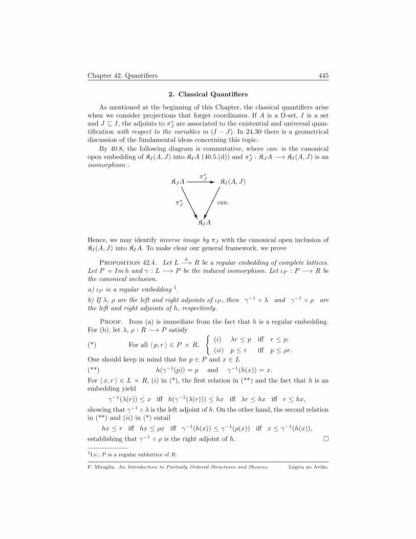
Chapter 42. Quantifiers 445
2. Classical Quantifiers
As mentioned at the beginning of this Chapter, the classical quantifiers arisewhen we consider projections that forget coordinates. If A is a Ω-set, I is a setand J ⊆ I, the adjoints to π∗J are associated to the existential and universal quan-tification with respect to the variables in (I − J). In 24.30 there is a geometricaldiscussion of the fundamental ideas concerning this topic.
By 40.8, the following diagram is commutative, where can. is the canonicalopen embedding of KI(A, J) into KIA (40.5.(d)) and π∗J : KJA −→ KI(A, J) is anisomorphism :
KJA - KI(A, J)
π∗J can.
KIA
π∗J
AAAAAU
Hence, we may identify inverse image by πJ with the canonical open inclusion ofKI(A, J) into KIA. To make clear our general framework, we prove
Proposition 42.4. Let Lh−→ R be a regular embedding of complete lattices.
Let P = Imh and γ : L −→ P be the induced isomorphism. Let ιP : P −→ R bethe canonical inclusion.
a) ιP is a regular embedding 1.
b) If λ, ρ are the left and right adjoints of ιP , then γ−1 λ and γ−1 ρ arethe left and right adjoints of h, respectively.
Proof. Item (a) is immediate from the fact that h is a regular embedding.For (b), let λ, ρ : R −→ P satisfy
(*) For all 〈 p, r 〉 ∈ P × R,
(i) λr ≤ p iff r ≤ p;
(ii) p ≤ r iff p ≤ ρr.
One should keep in mind that for p ∈ P and x ∈ L(**) h(γ−1(p)) = p and γ−1(h(x)) = x.
For 〈x, r 〉 ∈ L × R, (i) in (*), the first relation in (**) and the fact that h is anembedding yield
γ−1(λ(r)) ≤ x iff h(γ−1(λ(r))) ≤ hx iff λr ≤ hx iff r ≤ hx,
showing that γ−1 λ is the left adjoint of h. On the other hand, the second relationin (**) and (ii) in (*) entail
hx ≤ r iff hx ≤ ρx iff γ−1(h(x)) ≤ γ−1(ρ(x)) iff x ≤ γ−1(h(x)),
establishing that γ−1 ρ is the right adjoint of h.
1I.e., P is a regular sublattice of R.
F. Miraglia. An Introduction to Partially Ordered Structures and Sheaves. Logica no Aviao.
Chapter 42. Quantifiers 446
Proposition 42.4 shows that if the regular embedding h is identified, via theisomorphism γ, to the canonical embedding of its image into its codomain, thenthe left and right adjoints of this embedding are isomorphic to the left and rightadjoints of h, respectively.
Applying 42.4 to the open embedding π∗J : KJA −→ KIA, we obtain thatthe left and right adjoints of the canonical inclusion of KI(A, J) into KIA willrepresent, up to isomorphism, the left and right adjoints of π∗J . This is the way weshall treat the classical quantifiers.
42.5. Notation. If A is a Ω-set, K ⊆ I are sets and a ∈ |A|I , define
p(a,K) = c ∈ |A|I : πK(a) = πK(c). 2
Theorem 42.6. Let A be a Ω-set, and J ⊆ I be sets. For S in KIA and a in|A|I , define
(∃πJ) [[∃πJS(a) ]] = Ea ∧∨c∈p(a,J) [[S(c) ]];
(∀πJ) [[∀πJS(a) ]] = Ea ∧∧c∈p(a,J) Ec → [[S(c) ]],
where → in the right-hand side of (∀πJ) is implication in Ω. Then,
a) S ∈ KI(A,K) ⇒ ∃πJS, ∀πJS ∈ KI(A, K ∩ J).
b) The map ∃πJ , ∀πJ : KIA −→ KIA are the left and right adjoints of thecanonical inclusion of KI(A, J) into KIA, respectively.
Proof. Initially, it must be shown that if S ∈ KIA, then ∀πJS, ∃πJS ∈ KIA.The case of ∃πJS was treated in the proof of 40.8. In the case of ∀πJS, [ch 1] in37.1 is clear. For [ch 2], if x, y ∈ |A|I , it must be verified that
[[x = y]] ∧ [[ ∀πJS(x) ]] ≤ Ey ∧∧v∈p(y,J) Ev −→ [[S(v) ]],
that amounts to proving that for each v ∈ p(y, J)
[[x = y]] ∧ [[ ∀πJS(x) ]] ≤ Ev −→ [[S(v) ]],
that, in view of the adjunction [→] in 6.1, reduces to
(1) [[x = y]] ∧ [[ ∀πJS(x) ]] ∧ Ev ≤ [[S(v) ]].
Notation as in 37.24, set c = 〈πJ(x);πJ−I(v) 〉; then, c ∈ p(x, J) and, sinceπJ(v) = πJ(y), [=J ] in 38.9 yields
(2)[[c = v]] = [[πJ(x) = πJ(v)]] ∧ [[πI−J(v) = πI−J(v)]]
= [[πJ(x) = πJ(y)]] ∧ EπI−J(v).
From (2), we obtain, recalling [EJ ] and [=J ] in 38.9,
[[x = y]] ∧ Ev =
= [[πJ(x) = πJ(y)]] ∧ [[πJ−I(x) = πI−J(y)]] ∧ EπJ(v) ∧ EπI−J(v)
= [[c = v]] ∧ [[πJ−I(x) = πI−J(y)]] ∧ EπJ(v)
= [[c = v]] ∧ [[πI−J(x) = πI−J(y)]] ≤ [[c = v]].
Going back to (1), the preceding and Modus Ponens in 6.4.(b) entail
F. Miraglia. An Introduction to Partially Ordered Structures and Sheaves. Logica no Aviao.
Chapter 42. Quantifiers 447
[[x = y]] ∧ [[ ∀πJS(x) ]] ∧ Ev ≤ [[c = v]] ∧ Ex ∧∧u∈p(x,J) Eu → [[S(u) ]]
≤ [[c = v]] ∧ (Ec → [[S(c) ]])
= Ec ∧ [[c = v]] ∧ (Ec → [[S(c) ]])
≤ [[c = v]] ∧ [[S(c) ]] ≤ [[S(v) ]]
completing the proof that ∀πJS ∈ KIA.
a) Let S ∈ KI(A,K) and x, y ∈ |A|I verify J ⊆ c(x, y). It must be shown (40.2.(a))that
(3) Ex ∧ [[ ∀πJS(y) ]] = Ey ∧ [[ ∀πJS(x) ]].
Fact 1. For x, y as above, if u ∈ p(x, J), then
Eu ∧ [[ ∀πJS(y) ]] ≤ [[S(u) ]].
Proof. Set c = 〈πJ(y); πJc(u) 〉; note that c ∈ p(y, J) and
(i) Ec = EπJ(y) ∧ EπJc(u) ≥ Ey ∧ Eu;
(ii) c(c, u) = I; indeed, outside J , c and u coincide, while in J we have πJc = πJyand πJu = πJx, and so J ⊆ c(c, u).
(iii) By 40.3.(a), (ii) implies Eu ∧ [[S(c) ]] = Ec ∧ [[S(u) ]].
From (i) and (iii) we get
Eu ∧ [[ ∀πJS(y) ]] = Eu ∧ Ey ∧∧v∈p(y,J) Ev → [[S(v) ]]
≤ Ec ∧ Eu ∧ (Ec → [[S(c) ]])
≤ Eu ∧ [[S(c) ]] ≤ [[S(u) ]],
completing the proof of Fact 1.
By Fact 1, for all u ∈ p(x, J) we have [[∀πJS(y) ]] ≤ Eu → [[S(u) ]], and so,taking meets with respect to u on the right-hand side and meets with Ex on bothsides, we arrive at Ex ∧ [[ ∀πJS(y) ]] ≤ [[ ∀πJS(x) ]], which in turn readily impliesEx ∧ [[ ∀πJS(y) ]] ≤ Ey ∧ [[ ∀πJS)(x) ]]. Since the argument is symmetrical in xand y, we conclude the validity of (3). The argument for ∃πJ is similar (in fact,simpler).
b) It is immediate from (a) that ∀πJS, ∃πJS ∈ KI(A, J), for all S in KIA. LetιJ : KI(A, J) −→ KIA be the natural embedding.
∀πJ is right adjoint to ιJ : For R ∈ KI(A, J) and S ∈ KIA, we must verify that
(4) R ≤ S ⇔ R ≤ ∀πJS.
Assume that [[R(x) ]] ≤ [[S(x) ]], for all x ∈ |A|I . If u ∈ p(x, J), the fact thatR ∈ KI(A, J) entails Eu ∧ [[R(x) ]] = Ex ∧ [[R(u) ]] ≤ [[S(u) ]], whence[[R(x) ]] ≤ Eu → [[S(u) ]]. Since u is arbitrary in p(x, J) and [[R(x) ]] ≤ Ex, weget
[[R(x) ]] ≤ Ex ∧∧u∈p(x,J) Eu → [[S(u) ]] = [[∀πJS(x) ]],
verifying (⇒) in (4). Conversely, if the right-hand side of (4) holds, then
[[R(x) ]] ≤ Ex ∧ (Ex → [[S(x) ]]) ≤ [[S(x) ]],
as needed.
∃πJ is left adjoint to ιJ : This amounts to proving, for R ∈ KI(A, J) and S ∈ KIA
F. Miraglia. An Introduction to Partially Ordered Structures and Sheaves. Logica no Aviao.

Chapter 42. Quantifiers 448
∃πJS ≤ R ⇔ S ≤ R.
(⇒) is clear; for the converse, fix x ∈ |A|I . If u ∈ p(x, J), then
Ex ∧ [[S(u) ]] ≤ Ex ∧ [[R(u) ]] = Eu ∧ [[R(x) ]] ≤ [[R(x) ]].
Taking joins on both sides with respect to u ∈ p(x, J), we get
[[ ∃πJS(x) ]] ≤ [[R(x) ]],
ending the proof.
Corollary 42.7. Let A be a Ω-set and J ⊆ K ⊆ I be sets.
a) If R ∈ KI(A, J), then R = ∀πKR = ∃πKR.
b) If S ∈ KIA, then QπK (Q′πJ S) = Q′πJ S, where QπK and Q′πJ stand forexistential or universal quantification.
Proof. a) To be precise, let ιJ : KI(A, J) −→ KIA be the canonical embed-ding. We have a commutative diagram of open embeddings
KI(A, J) - KI(A,K)
ιJ ιK
KIA
ιJK
AAAAAU
and so ιK ιJK = ιJ . To simplify notation, let λK , ρK be the left and rightadjoints of ιK . Then, Corollary 7.9 yields
(*) λK ιK = IdKI(A,J) = ρK ιK .
Indeed, since 〈λJ , ιJ 〉 is an adjoint pair and ιJ is injective, 7.9.(a) entails λK ιJ = IdKI(A,J). Similarly, 7.9.(b) implies the other relation in (*). From (*), weobtain
λK ιJ = λK (ιK ιJK) = IdKI(A,J) ιJK = ιJK .
The same argument shows that ρK ιJ = ιJK , establishing (a). Item (b) followsreadily from (a) and 42.6.(a).
Corollary 42.7 expresses a familiar law of Logic : quantifying over variablesalready quantified yields nothing new. Another of these well-known laws is that theorder which variables are existentially or universally quantified is immaterial. Thiscan be proven by direct computation, but we prefer to use a different approach,that exhibits the structural properties of the concepts in discussion.
Proposition 42.8. a) A commutative diagram of regular embeddings of com-plete lattices
F. Miraglia. An Introduction to Partially Ordered Structures and Sheaves. Logica no Aviao.
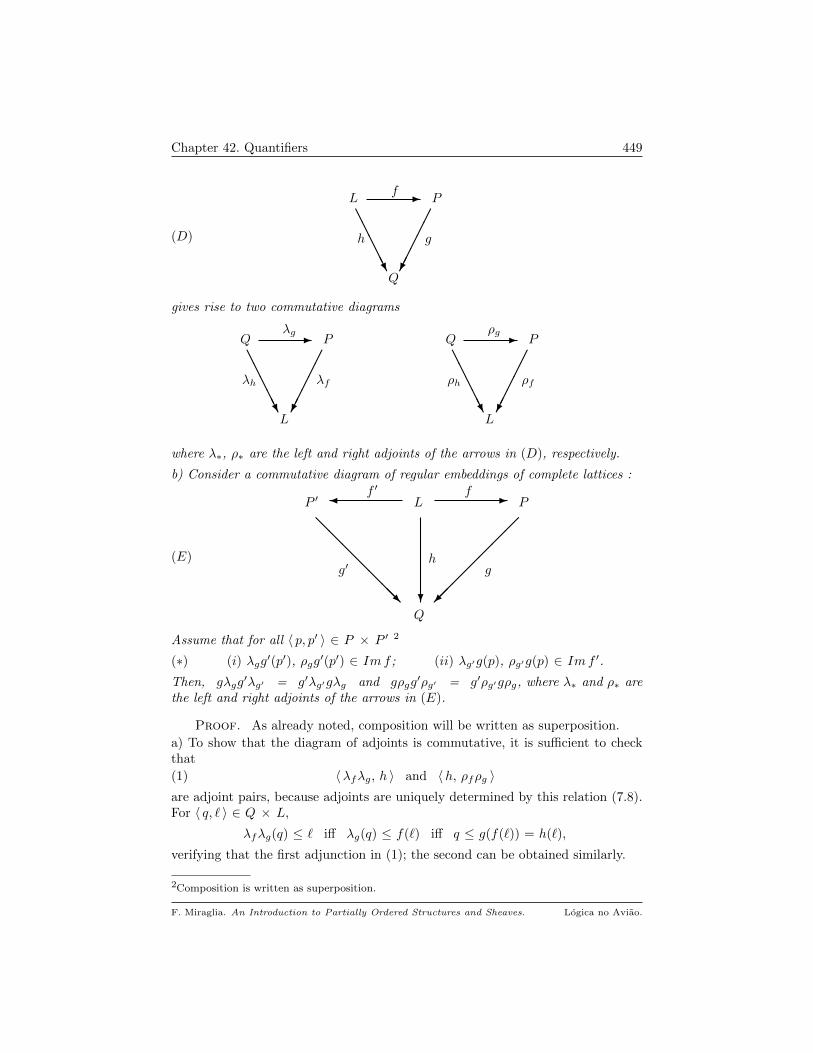
Chapter 42. Quantifiers 449
(D)
L - P
h g
Q
f
AAAAAU
gives rise to two commutative diagrams
Q - P
λh λf
L
λg
AAAAAU
Q - P
ρh ρf
L
ρg
AAAAAU
where λ∗, ρ∗ are the left and right adjoints of the arrows in (D), respectively.
b) Consider a commutative diagram of regular embeddings of complete lattices :
(E)
Q
L
?
h
- PP ′f ′ f
@@@@@@@R
g′
g
Assume that for all 〈 p, p′ 〉 ∈ P × P ′ 2
(∗) (i) λgg′(p′), ρgg
′(p′) ∈ Imf ; (ii) λg′g(p), ρg′g(p) ∈ Imf ′.
Then, gλgg′λg′ = g′λg′gλg and gρgg
′ρg′ = g′ρg′gρg, where λ∗ and ρ∗ arethe left and right adjoints of the arrows in (E).
Proof. As already noted, composition will be written as superposition.
a) To show that the diagram of adjoints is commutative, it is sufficient to checkthat
(1) 〈λfλg, h 〉 and 〈h, ρfρg 〉are adjoint pairs, because adjoints are uniquely determined by this relation (7.8).For 〈 q, ` 〉 ∈ Q × L,
λfλg(q) ≤ ` iff λg(q) ≤ f(`) iff q ≤ g(f(`)) = h(`),
verifying that the first adjunction in (1); the second can be obtained similarly.
2Composition is written as superposition.
F. Miraglia. An Introduction to Partially Ordered Structures and Sheaves. Logica no Aviao.

Chapter 42. Quantifiers 450
b) Since all arrows in (E) are injective, it follows from items (a) and (b) in 7.9that
(**) λ∗ ∗ = Iddom ∗ = ρ∗ ∗ .
We start with the following
Fact. 1) λgg′ = fλf ′ and ρgg
′ = fρf ′ . 2) λg′g = f ′λf and ρg′g = f ′ρf .
Proof. 1) We shall show that hypothesis (i) in (*) implies (1). For the first equation,let p′ be an element in P ′ and set λgg
′(p′) = f(`); then, (**) yields
` = λff(`) = λfλgg′(p′).
Hence, (a) and another application of (**) entail
λgg′(p′) = fλfλgg
′(p′) = fλhg′(p′) = fλf ′λg′g
′(p′) = fλf ′(p′),
as desired. The second equation in (1), as well as, the implication (∗).(ii) ⇒ (2)can be obtained similarly.
The first equation in (1) of the Fact and item(a) yield
λgg′ = fλf ′ ⇒ gλgg
′λg′ = gfλf ′λg′ = hλh.
Similarly, the first equation in (2) of the Fact entails
g′λg′gλg = hλh,
wherefrom we conclude that gλgg′λg′ = g′λg′gλg. The same argument applied to
the second equations in (1) and (2) of the Fact shows that
gρgg′ρg′ = hρh = g′ρg′gρg,
ending the proof.
Corollary 42.9. If A is a Ω-set and J , K ⊆ I are sets, then
QπJQπK = QπKQπJ ,
where Q is either ∃ or ∀.
Proof. By 42.6.(a), the following commutative diagram of open embeddingsverifies the hypothesis (i) and (ii) in (∗) of 42.8 :
KIA
KI(A, J ∩ K)
?
ιJ∩K
- KI(A, J)KI(A,K)ιJ∩K,K ιJ∩K,J
HHHHHH
HHHHHHHj
ιK
ιJ
Indeed, if R ∈ KI(A,K), then QπJR is in KI(A, J ∩K); of course, the same applies,with the roles of J and K reversed and the conclusion follows from 42.8.
Proposition 42.2.(c) applied to the open embedding ιJ : KI(A, J) −→ KIAyields (analogously to 42.3)
F. Miraglia. An Introduction to Partially Ordered Structures and Sheaves. Logica no Aviao.

Chapter 42. Quantifiers 451
Corollary 42.10. If A is a Ω-set, J ⊆ I are sets and R, S ∈ KIA,
a) ∀πJ(R → S) ≤ ∀πJR → ∀πJS.
b) ∀πJ¬R = ¬∃πJ¬¬R and ∀πJ¬¬R = ¬∃πJ¬R.
c) ¬∀πJ¬R = ¬¬∃πJ¬¬S.
d) R ∈ KI(A,K) ⇒ ∀vi¬R ∈ Reg(KI(A, (K − J)). 2
All the intuitionistic laws involving negation and quantifiers follow from 42.10.
The classical quantifiers along the ith-coordinate, ∃vi, ∀vi, are special cases ofthe above, with J = I − i. Here, instead of the p notation in 42.5, it is betterto use the substitution of an element of |A| into the ith-coordinate of a I-sequence,introduced in 37.10.(b). This is because for x ∈ |A|I ,
p(x, I − i) = x pa | iq ∈ |A|I : a ∈ |A|.The formulas for ∃vi and ∀vi are so important that we state them explicitly.
Corollary 42.11. Let A be a Ω-set and I be a set.
a) For i ∈ I and S ∈ KIA,
(∃vi) [[∃viS(x) ]] = Ex ∧∨a∈|A| [[S(x pa | iq ) ]].
(∀vi) [[∀viS(x) ]] = Ex ∧∧a∈|A| Ea → [[S(x pa | iq ) ]]
= Ex ∧∧a∈|A| Ea →
(Ea ∧ [[S(x pa | iq ) ]]
).
b) S ∈ KI(A,K) ⇒ QviS ∈ KI(A,K − i).
Proof. Immediate from the preceding results. For (b), just note that sinceQvi corresponds to QπI−i, 42.6.(a) guarantees that for S ∈ KI(A,K), QviS isin KI(A,K ∩ I − i) = KI(A, K − i).
Proposition 42.12. Let L, R be frames and A, B be presheaves over L andR, respectively. Let f = 〈 f, λ 〉 : A −→ B be a morphism in pSh, with λ a framemorphism. Let I be a set and R ∈ KIB. With notation as in 39.1,
a) For all i ∈ I, f∗(∃viR) ≥ ∃vi f∗R and f∗(∀viR) ≤ ∀vi f∗R.
b) Assume that f verifies Eb =∨a∈|A| [[fa = b]] and ρ λ = IdL, where ρ is the
right adjoint of λ.
(1) If ρ is a∨
-morphism, then f∗(∃viR) = ∃vi f∗R.
(2) If ρ is an open morphism, then f∗(∀viR) = ∀vi f∗R.
Proof. a) Let ρ : R −→ L be the right adjoint of λ. We shall use the followingobservations, all straightforward :
∗ If g : L −→ R is increasing and S ⊆ L, then g(∨S) ≥
∨s∈S g(s);
∗ g : L −→ R is a semilattice morphism, then g(p → q) ≤ g(p) → g(q).
One should also keep in mind that ρ λ ≥ IdL (7.8.(a)).
We first treat the case of the universal quantifier.
F. Miraglia. An Introduction to Partially Ordered Structures and Sheaves. Logica no Aviao.
Chapter 42. Quantifiers 452
Fact 42.13. For x ∈ |A|I , i ∈ I, a ∈ |A| and R ∈ KIB
Ex ∧ ρ(Efa → [[R(fx pa | iq ) ]]
)≤ Ea → f∗R(x pa|iq )
Proof. Since Efa = λ(Ea), by the second observation in the beginning of the proof,it is enough to check that
Ex ∧(ρ(λ(Ea)) → ρ
([[R(fx pa | iq ) ]]
))≤ Ea → f∗R(x pa | iq ).
By the adjunction [→] in 6.1, this is equivalent to
Ea ∧ Ex ∧(ρ(λ(Ea)) → ρ
([[R(fx pa | iq ) ]]
))≤ f∗R(x pa | iq ).
Since Ea ≤ ρ(λ(Ea)), Modus Ponens and 37.11.(a).(3) yield
Ea ∧ Ex ∧(ρ(λ(Ea)) → ρ
([[R(fx pa | iq ) ]]
))=
= Ea ∧ Ex ∧ ρ(λ(Ea)) ∧(ρ(λ(Ea)) → ρ
([[R(fx pa | iq ) ]]
))≤ Ea ∧ Ex ∧ ρ
(([[R(fx pa | iq ) ]]
)= Ex ∧ Ex pa | iq ∧ ρ
(([[R(fx pa | iq ) ]]
)≤ Ex pa | iq ∧ ρ
(([[R(fx pa | iq ) ]]
)= f∗R(x pa | iq ),
establishing the Fact.
Since ρ is a∧
-morphism we then obtain
f∗(∀viR)(x) = Ex ∧ ρ(
[[ ∀viR(fx) ]])
= Ex ∧ ρ(Efx ∧
∧y∈|B| Ey → [[R([fx] py | iq ) ]]
)= Ex ∧
∧y∈|B| ρ
(Ey → [[R([fx] py | iq ) ]]
)≤ Ex ∧
∧a∈|A| ρ
(Efa → [[R([fx] pfa | iq ) ]]
)≤ Ex ∧
∧a∈|A| Ea → f∗R(x pa | iq ) = ∀vi f∗R(x),
as needed. For the existential quantifier, 42.11 and 37.11.(a).(3) yield
f∗(∃viR)(x) = Ex ∧ ρ([[ ∃viR(fa) ]])
= Ex ∧ ρ(∨
y∈|B| Ey ∧ [[R([fx] py | iq ) ]])
≥ Ex ∧ ρ(∨
a∈|A| Efa ∧ [[R([fx] pfa | iq ) ]])
≥ Ex ∧ ρ(∨
a∈|A| λ(Ea) ∧ [[R(fx pa | iq ) ]])
≥ Ex ∧∨a∈|A| ρ(λ(Ea)) ∧ ρ
([[R(fx pa | iq ) ]]
)≥ Ex ∧
∨a∈|A| Ex ∧ Ea ∧ ρ
([[R(fx pa | iq ) ]]
)= Ex ∧
∨a∈|A| Ex pa | iq ∧ ρ
([[R(fx pa | iq ) ]]
)= Ex ∧
∨a∈|A| f
∗R(x pa | iq ) = ∃vi f∗R(x).
F. Miraglia. An Introduction to Partially Ordered Structures and Sheaves. Logica no Aviao.
Chapter 42. Quantifiers 453
b) (1) First note that for a ∈ |A|I and b ∈ |B|,[[R(fa pb | iq ) ]] = [[R(fa pb | iq ) ]] ∧ Eb
= [[R(fa pb | iq ) ]] ∧∨c∈|A| [[fc = b]]
=∨c∈|A| [[R(fa pb | iq ) ]] ∧ [[fc = b]]
=∨c∈|A| [[R(f(a pc | iq )) ]] ∧ [[fc = b]].
Hence, since ρ(Efc) = ρ(λ(Ec)) = Ec,
f∗(∃viR)(a) = Ea ∧ ρ([[ ∃viR(a) ]])
= Ea ∧ ρ(∨
b∈|B| [[R(fa pb | iq ) ]])
= Ea ∧∨b∈|B| ρ([[Rf(a pb | iq ) ]])
= Ea ∧∨b∈|B|
∨c∈|A| ρ([[R(f(a pc | iq )) ]] ∧ [[fc = b]])
= Ea ∧∨c∈|A| ρ
([[R(f(a pc | iq )) ]]) ∧
∨b∈|B| [[fc = b]]
)= Ea ∧
∨c∈|A| ρ([[R(f(a pc | iq )) ]]) ∧ ρ(Efc)
= Ea ∧∨c∈|A| ρ([[R(f(a pc | iq )) ]]) ∧ Ec
= Ea ∧∨c∈|A| Ea pc | iq ∧ ρ([[R(f(a pc | iq )) ]] = ∃vif∗R(a).
(2) For the universal quantifier, recall (8.16.(b)) that
(*)(∨
λ∈Λ pλ)→ q =
∧λ∈Λ (pλ → q).
Since Eb =∨c∈|A| [[fc = b]], (*) yields
Eb → [[R(fa pb | iq ) ]] = (∨c∈|A| [[fc = b]]) → [[R(fa pb | iq ) ]]
=∧c∈|A| [[fc = b]] → [[R(fa pb | iq ) ]]
=∧c∈|A| [[fc = b]] → ([[fc = b]] ∧ [[R(fa pb | iq ) ]])
=∧c∈|A| [[fc = b]] → ([[fc = b]] ∧ [[R(fa pfc | iq ) ]])
=∧c∈|A| [[fc = b]] → [[R(f(a pc | iq )) ]].
Thus, another application of (*) entails∧b∈|B| Eb → [[R(fa pb | iq ) ]] =
=∧b∈|B|
∧c∈|A| ([[fc = b]] → [[R(f(a pc | iq )) ]])
=∧c∈|A|
∧b∈|B| ([[fc = b]] → [[R(f(a pc | iq )) ]])
=∧c∈|A|
(∨b∈|B| [[fc = b]]
)→ [[R(f(a pc | iq )) ]]
=∧c∈|A| Efc → [[R(f(a pc | iq )) ]].
Since ρ is open and ρ(Efc) = Ec, we then obtain∧b∈|B| ρ(Eb → [[R(fa pb | iq ) ]]) =
∧c∈|A| Ec → ρ([[R(f(a pc | iq )) ]]),
and the conclusion in (2) is immediately forthcoming.
For localization at the filter of dense elements and regularization by doublenegation we have, complementing 39.3 and 39.5 :
Theorem 42.14. Let A be a Ω-presheaf and I 6= ∅ be a finite set. Let
h = 〈 εD, πD 〉 : A −→ A/D and Ar−→ rA
F. Miraglia. An Introduction to Partially Ordered Structures and Sheaves. Logica no Aviao.

Chapter 42. Quantifiers 454
be the localization of A at the filter D of dense elements in Ω (34.6, 39.3) and theregularization associated to double negation (35.7, 39.5).
a) For T ∈ KI(rA),
(1) r∗∀vi¬T = ∀vir∗¬T ;
(2) r∗¬∃viT = ¬∃vir∗T .
b) If T ∈ Reg(KI(rA)), then r∗(∀viT ) = ∀vir∗T .
c) For T ∈ KI(A/D),
(1) h∗∀vi¬T = ∀vi¬ h∗T ;
(2) h∗¬∃viT = ¬∃vih∗T .
d) If T ∈ Reg(KI(A/D)), then h∗∀viT = ∀vih∗T .
Proof. We prove (a) and (b), leaving (c), (d) to the reader. Recall thefollowing facts concerning implication and negation in a frame :
∗ p ∧ (q → r) = p ∧ ((p ∧ q) → (p ∧ r)); (6.4.(i))
∗ p ∧ q = p → (p ∧ q);∗ ¬¬ distributes over ∧ and →; (6.8.(g), 6.8.(j))
∗ q ∈ Reg(Ω) ⇒ p → q = ¬¬ p → q ∈ Reg(Ω); (6.20.(b))
∗ ¬¬∧s∈S ¬¬ s =
∧s∈S ¬¬ s; (8.16.(g))
∗ ¬ (∨S) = ¬
∨s∈S ¬¬ s; (8.16.(h))
These relations will be used forthwith, without comment.
Fact 42.15. For 〈x, p 〉 ∈ |rA|, a ∈ |A|I and T ∈ KI(rA)
¬ [[T ([ra] p〈x, p 〉 | iq ) ]] = ¬ [[T (r(a px | iq )) ]].
Proof. From Fact 39.6.(a) comes
[[T (r(a px | iq )) ]] =∧j 6=i Eaj ∧ Ex ∧ [[T ([ra] p〈x, p 〉 | iq ) ]].
Taking double negation on both sides, recalling that Ex ≤ p ≤ ¬¬Ex, we get
¬¬ [[T (r(a px | iq )) ]] =∧i6=j ¬¬Eaj ∧ ¬¬Ex ∧ ¬¬ [[T ([ra] p〈x, p 〉 | iq ) ]]
= ¬¬E[ra] p〈x, p 〉 | iq ∧ ¬¬ [[T ([ra] p〈x, p 〉 | iq ) ]]
= ¬¬ [[T ([ra] p〈x, p 〉 | iq ) ]],
which is equivalent to the desired result.
Proof of (1) : From 42.15 we get, since Ea = Era and E〈x, p 〉 = p (35.1) :
r∗(∀vi¬T )(a) = [[∀vi¬T (ra) ]]
= Ea ∧∧〈x,p〉∈|rA| E〈x, p 〉 → [[¬T ([ra] p〈x, p 〉 | iq ) ]]
= Ea ∧∧〈x,p〉∈|rA| p → E[ra] p〈x, p 〉 | iq ∧ ¬ [[T ([ra] p〈x, p 〉 | iq ) ]]
= Ea ∧∧〈x,p〉∈|rA| (Ea ∧ p) →
→ Ea ∧ E[ra] p〈x, p 〉 | iq ∧ ¬ [[T (r(a p〈x, p 〉 | iq ) ]].
By Lemma 37.11.(a).(3), we have
Ea ∧ E[ra] p〈x, p 〉 | iq = Era ∧ E[ra] p〈x, p 〉 | iq = Ea ∧ E〈x, p 〉 = Ea ∧ p,which substituted in the expression above yields
F. Miraglia. An Introduction to Partially Ordered Structures and Sheaves. Logica no Aviao.
Chapter 42. Quantifiers 455
(I)
r∗(∀vi¬T )(a) = Ea ∧∧〈x,p〉∈|rA| (Ea ∧ p) →
→ Ea ∧ p ∧ ¬ [[T (r(a px | iq )) ]]
= Ea ∧∧〈x,p〉∈|rA| p → ¬ [[T (r(a px | iq )) ]].
Since ¬ [[T (r(a px | iq )) ]] is regular in Ω, for 〈x, p 〉 ∈ |rA|, we have
p → ¬ [[T (r(a px | iq )) ]] = ¬¬ p → ¬ [[T (r(a px | iq )) ]]
= ¬¬Ex → ¬ [[T (r(a px | iq )) ]]
= Ex → ¬ [[T (r(a px | iq )) ]]
and so (I) leads to r∗(∀vi¬T )(a) = Ea ∧∧x∈|A| Ex → ¬ [[T (r(a px | iq )) ]]
= ∀vir∗¬T (a),
establishing (1). Item (b) is immediate from this and Theorem 39.5.
Proof of (2) : For a ∈ |A|I , 42.15 entails
r∗(¬∃viT )(a) = [[¬∃viT (ra) ]] = Ea ∧ ¬ [[ ∃viT (ra) ]]
= Ea ∧ ¬(∨〈x,p〉∈|rA| [[T ([ra] p〈x, p 〉 | iq ) ]]
)= Ea ∧ ¬
(∨〈x,p〉∈|rA| ¬¬ [[T ([ra] p〈x, p 〉 | iq ) ]]
)= Ea ∧ ¬
(∨〈x,p〉∈|rA| ¬¬ [[T (r(a px | iq )) ]]
)= Ea ∧ ¬
(∨x∈|A| [[T (r(a px | iq )) ]]
)= ¬∃vir∗T (a),
ending the proof.
Exercises
42.16. Let A be a Ω-presheaf and E : A−→ 1 be the unique presheaf morphismfrom A to the final object 1 (25.5, 26.10). Let S be a closed subpresheaf of A andp ∈ Ω.
a) The following are equivalent :
(1) ∃ES = p; (2) ES = p 3;
(3) ∃ pi : i ∈ I ⊆ p with p =∨i∈I pi and S(pi) 6= ∅, ∀ i ∈ I.
b) The following are equivalent :
(1) ¬ [[S = ∅]] = p 4.
(2) p =∨q ∈ Ω :
∀ r ≤ q, if r 6= ⊥, there is ⊥ 6= r′ ≤ r,
such that S(r′) 6= ∅.
(3) p ∈ Reg(Ω), ES ≤ p and there is a q ≤ p, such that ¬¬ q = p and
S(q) 6= ∅.c) What can be said about the relation between the following elements of Ω : ∃ESand [[S 6= ∅ ]] =def ¬ [[S = ∅]] ? 2
3ES is the support of S, as in 26.1.(c).4∅ is the empty subpresheaf of A; this equality is defined in 36.6.
F. Miraglia. An Introduction to Partially Ordered Structures and Sheaves. Logica no Aviao.

CHAPTER 43
Relations. Equivalence Relations and Quotients
As in section 24.3, a relation on presheaves A1, . . . , An is a subpresheaf of∏Ai. Since we are mainly interested in the subobjects describable via character-
istic maps, we define a relation on A1, . . . , An as a closed subpresheaf of∏Ai.
Any set of sections in this product generates a relation on A1, . . . , An : its closurein∏Ai. Notice that this automatically prescribes that a relation on a finite family
of sheaves is a subsheaf of their product.
Definition 43.1. Let n ≥ 1 be an integer. A n-ary relation on a Ω-presheafA is a characteristic map in KnA. If R is a binary relation on A, that is R ∈ K2A,we frequently use the so called infix notation for R, that is,
[[x R y ]] stands for [[R(x, y) ]].
All subsets S ⊆ |An| generate a n-ary relation on A, namely [[S(∗) ]].
Lemma 43.2. Let A be a L-set. For R ∈ KnA, n ≥ 2, the following areequivalent 1 :
(1) For all x ∈ |A|n, [[ ∆n(x) ]] ≤ [[R(x) ]];
(2) For all a ∈ |A|, [[R(a) ]] = Ea.
Proof. By 37.19, [[ ∆n(x) ]] =∧n−1i=1 [[xi = xi+1]], and (1) ⇒ (2) follows
immediately. For the converse, given x ∈ |A|n, formula (]) in the proof of 37.19(page 408), yields, with a = xn∧n−1i=1 [[xi = xi+1]] = Exn ∧
∧n−1i=1 [[xi = xi+1]]
= Exn ∧∧ni=1 [[xn = xi]]
= [[R(xn) ]] ∧∧ni=1 [[xn = xi]] ≤ [[R(x) ]],
as needed.
Definition 43.3. If R is a binary relation on A, define the inverse of R bythe rule
For all 〈x, y 〉 ∈ |A|2, [[ y R−1 x ]] = [[x R y ]].
Classically, an equivalence relation on a set A is a subset θ ⊆ A × A, suchthat ∆ ⊆ θ, θ = θ−1 and θ θ ⊆ θ. By analogy, we set down
1Notation as in 37.19; moreover, a = 〈 a, a, . . . , a 〉 ∈ An.
456
Chapter 43. Relations. Equivalence Relations and Quotients 457
Definition 43.4. An equivalence relation on a L-set A is a binary relationθ on A, such that for all x, y, z ∈ |A|
[ER 1] : [[x = y]] ≤ [[x θ y ]];
[ER 2] : [[x θ y ]] = [[ y θ x ]];
[ER 3] : [[x θ z ]] ∧ [[ z θ y ]] ≤ [[x θ y ]].
Write Eq(A) for the poset of equivalence relations on A, with the order inducedby K2A.
Remark 43.5. Let A be an L-set and θ ∈ Eq(A).
a) By 43.2, condition [ER 1] in 43.4 is equivalent to
[ER 1′] : ∀ x ∈ |A|, [[x θ x ]] = Ex.
Note the similarity of [ER 1′] to the usual reflexive law “x θ x”.
b) For x, y ∈ |A|, we have [[x = y]] ≤ [[x θ y ]] ≤ Ex ∧ Ey. It is clear that
[[x >2 y ]] = Ex ∧ Ey and [[x = y]],
are both equivalence relations on A, in fact, the top and bottom, respectively, ofthe poset Eq(A). Exercise 43.9 describes some of the lattice-theoretic propertiesof Eq(A). 2
Example 43.6. Let A be a Ω-set and p ∈ Ω. For x, y ∈ |A|, define
[[x θp y ]] = Ex ∧ Ey ∧ [p → (p ∧ [[x = y]])].
It is easily established that θp ∈ K2A and that it satisfies [ER 1′] in 43.5.(a) and[ER 2] in 43.4. Hence, to see that θp is an equivalence relation on A, it remains toverify transitivity; for x, y, z ∈ |A|, this comes down to
p ∧ Ex ∧ Ey ∧ Ez ∧ [[x θp y ]] ∧ [[ y θp z ]] ≤ p ∧ [[x = z]].
But the rule of Modus Ponens in 6.4 yields
p ∧ Ex ∧ Ey ∧ Ez ∧ [p → (p ∧ [[x = y]])] ∧ [p → (p → [[y = z]])] ≤≤ p ∧ ([[x = y]] ∧ [[y = z]]) ≤ p ∧ [[x = z]],
as needed. In the notation of 37.16, we have
Sθp = 〈 s, t 〉 ∈ |A2| : p ∧ Es ∧ Et = p ∧ [[s = t]],which, in case A is a Ω-presheaf, may be written
Sθp = 〈 s, t 〉 ∈ |A2| : s|p = t|p.
Hence, the equivalence relation θp corresponds to compatibility over p in A, asdefined in 25.26. 2
43.7. Quotients. If θ is an equivalence relation on an L-set A, let θ be thefollowing binary relation on |A| :
x θ y iff Ex = Ey = [[x θ y ]].
It is clear θ is an equivalence relation on |A|. Write x/θ for the class of x ∈ |A|with respect to θ. Define a L-set A/θ by the following prescriptions :
F. Miraglia. An Introduction to Partially Ordered Structures and Sheaves. Logica no Aviao.

Chapter 43. Relations. Equivalence Relations and Quotients 458
(i) |A/θ| = x/θ : x ∈ |A| = |A|/θ; (ii) [[x/θ = y/θ]] = [[x θ y ]].
Then A/θ is an extensional L-set and the natural map
πθ : |A| −→ |A/θ|, x 7−→ x/θ
is a morphism of L-sets. The diagram Aπθ−→ A/θ is the quotient of A by
the equivalence relation θ. The universal property of the diagram Aπθ−→ A/θ
appears in Exercise 43.10.
Now suppose A is a L-presheaf. For x, y ∈ |A| and p ∈ L,
(*) x θ y ⇒ x|p θ y|p.To see this, note that [[x|p θ x ]] ≥ [[x|p = x]] = p ∧ Ex, with a similar relation
holding with y in place of x. Thus, [ER 3] in 43.4 and the hypothesis that x θ yentail
[[x|p θ y|p ]] ≥ [[x|p θ x ]] ∧ [[x θ y ]] ∧ [[ y θ y|p ]] = p ∧ Ex ∧ Ey.
Since Ex|p = p ∧ Ex = p ∧ Ey = Ey|p and θ is a characteristic function, the
above inequality implies [[x|p θ y|p ]] = Ex|p = Ey|p, establishing (*). Since
θ is a congruence with respect to restriction, there is a natural way to make thequotient A/θ into a L-presheaf and πθ into a presheaf morphism : for x ∈ |A| andp ∈ L, define
(**) (x/θ)|p = x|p/θ.
The diagram Aπθ−→ A/θ is the quotient of A by θ in the category pSh(L). In
general. A/θ will not be a sheaf even if A is a sheaf. In this case, we definethe quotient of A by θ to be the completion of the presheaf constructedabove, still indicating it by A/θ. 2
As an application of equivalence relations, we prove a general result concerningthe gluing of families of presheaves. For topological spaces, this appears in section3.3 of Chapter 0 in [24] (and Exercise II.1.22 in [25]). This is the process by whicha general scheme is constructed out of affine schemes in Algebraic Geometry.
If p ∈ Ω, the ideal p← = q ∈ Ω : q ≤ p is a frame, with p in the role of >.The concept of restriction of a L-set A to an element p of L, A|p, was defined in
25.3. With these preliminaries, we state
Theorem 43.8. Let Ω be a frame and B be a subset of Ω. Suppose we aregiven the following data :
(1) For each b ∈ B, a presheaf Ab over b←;
(2) For each 〈 a, b 〉 ∈ B × B, an isomorphism fab : Aa|a∧b −→ Ab|a∧b, such that
for all a, b, c ∈ B we have, with p = a ∧ b ∧ c,a) fbb = IdAb .
b) If x ∈ |Aa| is such that Ex ≤ p, then fac(x) = [fbc fab](x).
F. Miraglia. An Introduction to Partially Ordered Structures and Sheaves. Logica no Aviao.
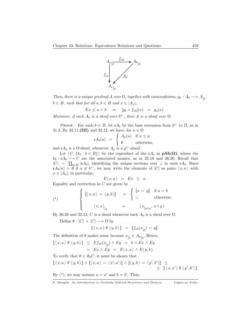
Chapter 43. Relations. Equivalence Relations and Quotients 459
Ac|p
Aa|p
?
- Ab|p
fac
fab
fbc
Then, there is a unique presheaf A over Ω, together with isomorphisms, gb : Ab −→ A|b,b ∈ B, such that for all a, b ∈ B and x ∈ |Aa|,
Ex ≤ a ∧ b ⇒ [gb fab](x) = ga(x).
Moreover, if each Ab is a sheaf over b←, then A is a sheaf over Ω.
Proof. For each b ∈ B, let eAb be the base extension from b← to Ω, as in31.3. By 32.11.(III) and 32.12, we have, for u ∈ Ω
eAb(u) =
Ap(u) if u ≤ p
∅ otherwise,
and eAp is a Ω-sheaf, whenever Ap is a p←-sheaf.
Let 〈C, kb : b ∈ B 〉 be the coproduct of the eAb in pSh(Ω), where thekb : eAb −→ C are the associated monics, as in 25.19 and 26.20. Recall that|C| =
∐b∈B |eAb|, identifying the unique sections over ⊥ in each eAb. Since
eAb(u) = ∅ if u 6∈ b←, we may write the elements of |C| as pairs 〈x, a 〉 withx ∈ |Aa|; in particular,
E〈x, a 〉 = Ex ≤ a.
Equality and restriction in C are given by
(*)
[[〈x, a 〉 = 〈 y, b 〉]] =
[[x = y]] if a = b
⊥ otherwise.
〈x, a 〉|q = 〈x|a∧q, a∧ q 〉.
By 26.20 and 32.12, C is a sheaf whenever each Ab is a sheaf over Ω.
Define θ : |C| × |C| −→ Ω by
[[ 〈x, a 〉 θ 〈 y, b 〉 ]] = [[fab(x|b) = y]].
The definition of θ makes sense because x|b ∈ Aa|b. Hence,
[[ 〈x, a 〉 θ 〈 y, b 〉 ]] ≤ Efab(x|b) ∧ Ey = b ∧ Ex ∧ Ey= Ex ∧ Ey = E〈x, a 〉 ∧ E〈 y, b 〉.
To verify that θ ∈ K2C, it must be shown that
[[ 〈x, a 〉 θ 〈 y, b 〉 ]] ∧ [[〈x, a 〉 = 〈x′, a′ 〉]] ∧ [[〈 y, b 〉 = 〈 y′, b′ 〉]] ≤≤ [[ 〈x, a′ 〉 θ 〈 y′, b′ 〉 ]].
By (*), we may assume a = a′ and b = b′. Thus,
F. Miraglia. An Introduction to Partially Ordered Structures and Sheaves. Logica no Aviao.

Chapter 43. Relations. Equivalence Relations and Quotients 460
[[fab(x|b) = y]] ∧ [[〈x, a 〉 = 〈x′, a 〉]] ∧ [[〈 y, b 〉 = 〈 y′, b 〉]]= [[fab(x|b) = y]] ∧ [[x = x′]] ∧ [[y = y′]]
≤ [[fab(x|b) = y]] ∧ b ∧ [[x = x′]] ∧ [[y = y′]]
= [[fab(x|b) = y]] ∧ [[x|b = x′|b]] ∧ [[y = y′]]
≤ [[fab(x|b) = y]] ∧ [[fab(x|b) = fab(x′|b)]] ∧ [[y = y′]]
≤ [[fab(x′|b) = y]] ∧ [[y = y′]] ≤ [[fab(x
′|b) = y′]]
and property [ch 2] in 37.1 follows immediately. It remains to check that θ is anequivalence relation on C. We have
∗ Property (a) in the statement implies [[ 〈x, a 〉 θ 〈x, a 〉 ]] = Ex; by 43.2, θverifies [ER 1] in 43.4;
∗ By (2).(b), fba restricted to Aa|a∧b has fab as its inverse. Thus, definition θ is
symmetrical, i.e., [[ 〈x, a 〉 θ 〈 y, b 〉 ]] = [[ 〈 y, b 〉 θ 〈x, a 〉 ]].∗ To check transitivity, let 〈x, a 〉, 〈 y, b 〉 and 〈 z, c 〉 be sections in |C|. Then, ifp = a ∧ b ∧ c, (2).(b) and 26.8.(b) yield
[[ 〈x, a 〉 θ 〈 y, b 〉 ]] ∧ [[ 〈 b, y 〉 θ 〈 z, c 〉 ]] =
= [[fab(x|b) = y]] ∧ [[fbc(y|c) = z]]
= p ∧ [[fab(x|b) = y]] ∧ [[fbc(y|c) = z]]
= [[fab(x|p) = y|p]] ∧ [[fbc(y|p) = z|p]]≤ [[fbc(fab(x|p)) = fbc(y|p)]] ∧ [[fbc(y|p) = z|p]]= [[fac(x|p) = fbc(y|p)]] ∧ [[fbc(y|p) = z|p]]≤ [[fac(x|p) = z|p]] = p ∧ [[fac(x|c) = z]]
≤ [[fac(x|c) = z]],
and so θ is transitive. Let A be the quotient presheaf C/θ and πθ : C −→ C/θ be
the quotient map. Recall (43.7) that the domain of C/θ is |A|/θ, where θ is theequivalence relation
〈 t, a 〉 θ 〈 z, b 〉 iff Et = Ez = [[fab(t|b) = z]].
Since Ab is extensional and Ez ≤ a ∧ b, this equivalence can be written 2
(+) 〈 t, a 〉 θ 〈 z, b 〉 iff fab(t) = z.
For b ∈ B, consider the presheaf morphisms gb = πθ kb : Ab −→ A; we shallprove that they satisfy the requirements in the conclusion of the Theorem.
If 〈 z, c 〉/θ ∈ |A|b|, then E〈 z, c 〉/θ = Ez ≤ b, and so Ez ≤ b ∧ c. Hence, (+)
entails 〈 z, c 〉 θ 〈 fcb(z), b 〉; therefore
πθ kb(fcb(z)) = πθ (〈 fcb(z), b 〉) = 〈 z, c 〉/θ,
2Because t|b = t.
F. Miraglia. An Introduction to Partially Ordered Structures and Sheaves. Logica no Aviao.
Chapter 43. Relations. Equivalence Relations and Quotients 461
and gb : Ap −→ A|p is surjective. For injectivity if x, y ∈ |Ab|, then 3,
[[gb(x) = gb(y)]] = [[〈x, b 〉/θ = 〈 y, b 〉/θ]] = [[ 〈x, b 〉 θ 〈 y, b 〉 ]]= [[fbb(x) = y]] = [[x = y]]
and the conclusion follows from 26.17.(b). To finish the proof in the presheaf case,
let a, b ∈ B and x ∈ |Aa| satisfy Ex ≤ a ∧ b. Then, since 〈x, a 〉 θ 〈 fab(x), b 〉) (by(+) above), we have
gb(fab(x))) = πθ(kb(fab(x))) = πθ(〈 fab(x), b 〉) = 〈 fab(x), b 〉)/θ= 〈x, a 〉/θ = ga(x),
as desired. The case in which Ab is a sheaf, b ∈ B, let cA be the completion ofthe presheaf A constructed above. If we substitute g∗ by c πθ k∗, we obtainmonics from A∗ into cA, with the properties in the statement. Since A|b ≈ Ab,
A|b is complete over all q ∈ p←. We now invoke Theorem 27.20 to conclude that
cA|b = A|b and the newly defined monics are in fact isomorphisms, ending the
proof.
The equivalence relation generated by a set of sections in |A × A| is instru-mental in proving that Ω set, pSh(Ω) and Sh(Ω) have coequalizers, as was thecase for sheaves and presheaves over topological spaces in section 24.3. The detailsare left as Exercise 43.11.
Exercises
43.9. Let A be a Ω-presheaf.
a) Eq(A) is a complete lattice with the po induced by K2A4. Is it a complete
sublattice of K2A ?
b) If S ⊆ |A2|, define the equivalence relation generated by S to be
[[x θS y ]] =∧[[x R y ]] :
R ∈ Eq(A) and ∀ 〈 s1, s2 〉 ∈ S[[ s1 R s2 ]] = Es1 = Es2
If S = 〈x, y 〉, write θxy for θS . Then,
(1) For all 〈x, y 〉 ∈ |A2|, θxy is compact in Eq(A).
(2) For all R ∈ Eq(A), R =∨〈x,y〉∈R θxy.
(3) Eq(A) is an algebraic frame. 2
43.10. a) Let A be an L-set and θ ∈ Eq(A). Let f : A −→ B be a morphismof L-sets, such that
∀ x, y ∈ |A|, [[x θ y ]] ≤ [[fx = fy]].
Then, there is a unique L-set morphism, g : A/θ −→ B satisfying g πθ = f .
3Recall (see (ii) in 43.7) that [[∗/θ = ∗/θ]] = [[ ∗ θ ∗ ]].4Hence, meets and joins are computed pointwise.
F. Miraglia. An Introduction to Partially Ordered Structures and Sheaves. Logica no Aviao.
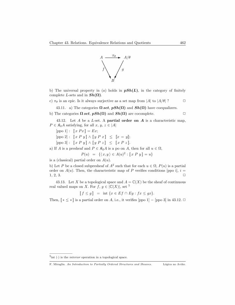
Chapter 43. Relations. Equivalence Relations and Quotients 462
A - A/θ
f g
B
πθ
AAAAAU
b) The universal property in (a) holds in pSh(L), in the category of finitelycomplete L-sets and in Sh(Ω).
c) πθ is an epic. Is it always surjective as a set map from |A| to |A/θ| ? 2
43.11. a) The categories Ω set, pSh(Ω) and Sh(Ω) have coequalizers.
b) The categories Ω set, pSh(Ω) and Sh(Ω) are cocomplete. 2
43.12. Let A be a L-set. A partial order on A is a characteristic map,P ∈ K2A satisfying, for all x, y, z ∈ |A|
[ppo 1] : [[x Px ]] = Ex;
[ppo 2] : [[x P y ]] ∧ [[ y P x ]] ≤ [[x = y]];
[ppo 3] : [[x P y ]] ∧ [[ y P z ]] ≤ [[x P z ]].
a) If A is a presheaf and P ∈ K2A is a po on A, then for all u ∈ Ω,
P (u) = 〈x, y 〉 ∈ A(u)2 : [[x P y ]] = uis a (classical) partial order on A(u).
b) Let P be a closed subpresheaf of A2 such that for each u ∈ Ω, P (u) is a partialorder on A(u). Then, the characteristic map of P verifies conditions [ppo i], i =1, 2, 3. 2
43.13. Let X be a topological space and A = C(X) be the sheaf of continuousreal valued maps on X. For f , g ∈ |C(X)|, set 5
[[ f ≤ g ]] = int x ∈ Ef ∩ Eg : fx ≤ gx.
Then, [[ ∗ ≤ ∗ ]] is a partial order on A, i.e., it verifies [ppo 1] − [ppo 3] in 43.12. 2
5int (·) is the interior operation in a topological space.
F. Miraglia. An Introduction to Partially Ordered Structures and Sheaves. Logica no Aviao.
CHAPTER 44
Finitary Relations and Operations on a Presheaf
This Chapter collects results on finitary relations and operations on Ω-presheaves,although many of them hold true for arbitrary Ω-sets.
Definition 44.1. If A is a Ω-presheaf, let 1
KfA =⋃J⊆fN KN(A, J); op(A) =
⋃J⊆fN [AI , A]J ,
be the set of finitary relations and operations, respectively, on A. For K ⊆f N,write op(A,K) for the operations on A that depend on K and op(A,n) for thosethat depend on n = 1, 2, . . . , n.
From Propositions 37.4 and 40.5 we get
Corollary 44.2. With the operations defined in 37.4, KfA is a Heytingalgebra, whose bottom is ⊥⊥⊥N and whose top is >>>N. Moreover, if Ω is a Booleanalgebra, the same is true of KfA.
In general, KfA is not a complete lattice for joins and meets of an arbitraryfamily of finitary relations might not be finitary. It will become apparent thatKfA and op(A) have just enough structure to interpret first-order Logic. We nowintroduce
Definition 44.3. For R ∈ KfA and ω ∈ op(A), define
fv(R) =⋂J ⊆ N : R depends on J
fv(ω) =⋂J ⊆ N : ω depends on J,
called the sets of free variables in R and ω, respectively.
Corollary 44.4. If R ∈ KfA and ω ∈ op(A), A a Ω-presheaf, then R dependson fv(R) and ω depends on fv(ω). Moreover, fv(∗) is the smallest subset of Non which ∗ depends.
Proof. Since R and ω depend on a finite subset of N, the intersectionsdefining fv(∗) in 44.3 are finite. The result is then a consequence of 40.5.(e).
The behavior of fv(∗) with respect to substitution and quantification is theusual one :
1Notation as in 40.2; recall that J ⊆f N means that J is a finite subset of N.
463
Chapter 44. Finitary Relations and Operations on a Presheaf 464
Corollary 44.5. Let A be a presheaf over Ω, R ∈ KfA and ω ∈ op(A). ForJ ⊆ N, let τ j, j ∈ J , be finitary operations in A and let τ be their product.
a) ∀ i ∈ N, ∃viR, ∀viR ∈ KfA and fv(∃viR) = fv(∀viR) = fv(R) − i.b) If J ⊆ fv(R), then R pτ | Jq ∈ KfA and
fv(R pτ | Jq ) = (fv(R) − J) ∪⋃j∈J fv(τ j).
c) If J ⊆ fv(ω), then ω pτ | Jq ∈ op(A) and
fv(ω pτ | Jq ) = (fv(ω) − J) ∪⋃j∈J fv(τ j).
Proof. Item (a) follows from Theorem 42.6.(a) (or 42.11.(b)). Items (b) and(c) are a consequence of Theorem 41.4.(b) and Proposition 41.7.
Let L, R be frames and A, B be presheaves over L, R, respectively. Letf = 〈 f, λ 〉 : A −→ B be a morphism in pSh, with λ a frame morphism. By Re-mark 40.9, image by f does not produce a morphism from KfA to KfB. However,for inverse image, we have
Corollary 44.6. With notation as above, let ρ be the right adjoint of λ.
a) f∗ : KfB −→ KfA is a semilattice morphism. If ρ preserves joins or implication,the same is true of f∗.
b) For T ∈ KfB, f∗(∃viR) ≥ ∃vi f∗R and f∗(∀viR) ≤ ∀vi f∗R.
c) If for all b ∈ |B|, Eb =∨c∈|A| [[fc = b]] and ρ λ = IdL, then
(1) ρ is a∨
-morphism ⇒ f∗(∃viR) = ∃vi f∗R.
(2) ρ is open ⇒ f∗(∀viR) = ∀vi f∗R.
Proof. a) By Proposition 40.10.(a), f∗ takes KfB to KfA. The preservationof meets, joins and implication follow from the corresponding assertions in 39.1.Items (b) and (c) are straightforward consequences of Proposition 42.12.
The next result is basic in connecting KfA and op(A) with the IntuitionisticPredicate Calculus H, presented in 17.5.
Proposition 44.7. Let A be a Ω-presheaf and J be a finite subset of N.Let ω, τ j ∈ op(A), j ∈ J , and let τ : AI −→ AJ be the product of the τ j. LetR, S ∈ KfA.
a) If 3 is one of the operations ∧, ∨ or →, then
(R 3 S) pτ | Jq = R pτ | Jq 3 S pτ | Jq .
Moreover, (¬R) pτ | Jq = ¬ (R pτ | Jq ).
b) If k 6∈ fv(τ) ∪ J , then
(∃vkR) pτ | Jq = ∃vk(R pτ | Jq );
(∀vkR) pτ | Jq = ∀vk(R pτ | Jq ).
c) For all k ∈ N, ∀vkR ≤ R pω | kq ≤ ∃vkR.
d) If k 6∈ fv(R), then for all x ∈ AN and c ∈ A(1) [[R(x) ]] ≤ [[S(x) ]] ⇒ Ec ∧ [[R(x) ]] ≤ [[S(x pc | kq ) ]].
F. Miraglia. An Introduction to Partially Ordered Structures and Sheaves. Logica no Aviao.
Chapter 44. Finitary Relations and Operations on a Presheaf 465
(2) [[S(x) ]] ≤ [[R(x) ]] ⇒ Ex ∧ [[S(x pc | kq ) ]] ≤ [[R(x) ]].
e) If k 6∈ fv(R), then
(1) R ≤ S ⇒ R ≤ ∀vkS; (2) S ≤ R ⇒ ∃vkS ≤ R.
Proof. a) All relations follow from 41.4.(b).(1). As an example, for implica-tion we have, with a ∈ |A|I , c = τ(a|Ea) and recalling that
Ea = Ea pτa|Ea | Jq = Ea pc | Jq ,
[[ (R → S) pτ | Jq (a) ]] = [[ (R → S)(a pc | Jq ) ]] =
= Ea pc | Jq ∧(
[[R(a pc | Jq ) ]] → [[S(a pc | Jq ) ]])
= Ea ∧ [[R pτ | Jq (a) ]] → [[S pτ | Jq (a) ]]
= [[ (R pτ | Jq → S pτ | Jq )(a) ]].
b) We treat the universal quantifier; the analogous argument for the existentialquantifier is left to the reader. For a ∈ |A|I and u ∈ |A|, set
x = a|Ea and yu = (a pu | kq )|Eapu|kq.
Then, x, yu ∈ AI , with
Ex = Ea and Eyu = Ea pu | kq =∧i 6=k Eai ∧ Eu.
Hence, Ex ∧ Eyu = Ea ∧ Eu. Since k 6∈ fv(τ) =⋃j∈J τ j (44.8.(d)), a and
a pu | kq coincide in all coordinates except k and
Ea|Ea∧Eu = E(a pu | kq )|Ea∧Eu = Ea ∧ Eu,
we conclude that
(*) τ(x)|Ea∧Eu = τ(x|Ea∧Eu) = τ(yu|Ea∧Eu) = τ(yu)|Ea∧Eu.
Hence, since k 6∈ J , 41.4.(b).(1) and (*) yield,
[[ (∀vk)R pτ | Jq (a) ]] = Ea ∧∧u∈|A| Eu → [[R pτ | Jq (a pu | kq ) ]]
= Ea ∧∧u∈|A| Eu → [[R(a pu | kq pτ(yu) | Jq ) ]]
= Ea ∧∧u∈|A| Ea ∧ Eu → Ea ∧ Eu ∧ [[R(a pu | kq pτ(yu) | Jq ) ]]
= Ea ∧∧u∈|A| Ea ∧ Eu → [[R(a pu | kq pτ(yu)|Ea∧Eu | Jq ) ]]
= Ea ∧∧u∈|A| Ea ∧ Eu → [[R(a pu | kq pτ(x)|Ea∧Eu | Jq ) ]]
= Ea ∧∧u∈|A| Ea ∧ Eu → Ea ∧ Eu ∧ [[R(a pu | kq pτ(x) | Jq ) ]]
= Ea ∧∧u∈|A| Ea ∧ Eu → Ea ∧ Eu ∧ [[R(a pτ(x) | Jq pu | kq ) ]]
= Ea ∧∧u∈|A| Eu → [[R(a pτ(x) | Jq pu | kq ) ]]
= Ea pτ(x) | Jq ∧∧u∈|A| Eu → [[R(a pτ(x) | Jq pu | kq ) ]]
= [[ (∀vkR) pτ | Jq (a) ]],
as desired.
c) For x ∈ |A|I , let c = ω(x|Ex). Then, Ec = Ex = Ex pc | kq . Hence, Theorem
41.4.(b).(1) yields
F. Miraglia. An Introduction to Partially Ordered Structures and Sheaves. Logica no Aviao.
Chapter 44. Finitary Relations and Operations on a Presheaf 466
[[ ∀vkS(x) ]] ≤ Ex ∧ (Ec −→ [[S(x pc | kq ) ]]) ≤ [[S(x pc | kq ) ]]
= [[S pω | kq (x) ]],
establishing the first inequality in (d). The second is similar.
d) For (1), since k 6∈ fv(R) it follows that
Ec ∧ [[R(x) ]] = Ec ∧∧i6=k Exi ∧ [[R(x) ]] = Ex pc | kq ∧ [[R(x) ]]
= Ex ∧ [[R(x pc | kq ) ]] ≤ Ex ∧ [[S(x pc | kq ]]
≤ [[S(x pc | kq ) ]].
Analogously, one obtains (2); item (e) is a straightforward consequence of (d) andthe pertinent definitions.
Exercises
44.8. Let A be a Ω-presheaf and R, S ∈ KfA. Let J ⊆f N, τ j ∈ op(A) andlet τ be the product of the τ j .
a) fv(R → S) = fv(R ∧ S) = fv(R ∨ S) = fv(R) ∪ fv(S).
b) fv(¬R) = fv(R).
c) fv(⊥⊥⊥N) = fv(>>>N) = ∅.d) Set fv(τ) =
⋂J ⊆ N : τ depends on J. Then, fv(τ) =
⋃j∈J fv(τ j). 2
44.9. Let A be a Ω-presheaf. All the axioms and rules of the IntuitionisticPropositional Calculus in 17.5 hold in KfA, with the following conventions :
∗ In the axioms and rules of H, the symbols φ, ψ and χ stand for elements of KfA;
∗ An axiom is satisfied if its value is >>>N for all φ, ψ, χ ∈ KfA;
∗ A rule is valid whenever the conjunction of its antecedents is satisfied, so is itsconclusion. For instance, to check that the rule of Modus Ponens is valid it mustbe shown that
φ ∧ (φ → ψ) = >>>N ⇒ ψ = >>>N,
for arbitrary φ, ψ in KfA. 2
F. Miraglia. An Introduction to Partially Ordered Structures and Sheaves. Logica no Aviao.

CHAPTER 45
Graded Frames
Let A be a Ω-presheaf. Recall (37.1) that if n ≥ 1 is an integer, KnA is theframe of n-characteristic maps on A. By Proposition 40.14, if J ⊆f N has cardinaln ≥ 1, there is an automorphism of KNA that takes KN(A, J) isomorphically ontoKN(A,n) 1, which may be identified with KnA (40.8). Hence, associated to A thereis a sequence of frames
K∗(A) = 〈K0(A), K1(A), . . . , Kn(A), . . . 〉where K0(A) = (EA)← (see (!) in 37.3). In this Chapter we introduce the structurethat is adequate to study this type of object. It is analogous to the graded rings andmodules that appear in Homology, Cohomology or in Topological and AlgebraicK-theory. A general reference for homological constructs is MacLane’s [45]; forAlgebraic K-theory the reader may consult [48], [4], [74] or [73]
1. Introduction
We start with the following
Definition 45.1. A graded frame is of a sequence of frames
L∗ = 〈L0, L1, . . . , Ln, . . . 〉together with a binary operation, ⊗ : L∗ × L∗ −→ L∗, consisting for each pair ofintegers n, m ≥ 0 of an operation
⊗ : Ln × Lm −→ Ln+m,
satisfying the following conditions, where ⊥n, >n are the top and bottom of Ln,respectively :
[⊗ 1] : ⊗ is associative;
[⊗ 2] : ⊗ distributes over finite meets and arbitrary joins;
[⊗ 3] : >n ⊗ >m = >m ⊗ >n = >n+m;
[⊗ 4] : For all η ∈ Ln, η ⊗ η = (η ⊗ >n) ∧ (>n ⊗ η);
[⊗ 5] : For all p ∈ L and η ∈ Ln, p ⊗ η = η ⊗ p = η ∧ (p ⊗ >n);
[⊗ 6] : For all η ∈ Ln, >0 ⊗ η = η ⊗ >0 = η.
The frame Ln is the component of degree n of L∗; a member of Ln iscalled an element of degree n of L∗. When context allows write > for >0
1n = 1, 2, . . . , n.
467
Chapter 45. Graded Frames 468
(the top of L0). A graded cBa is a graded frame in which all components arecomplete Boolean algebras.
The following comments are included to help make the statement of Definition45.1 clearer :
∗ The only commutativity assumptions are [⊗ 5] and [⊗ 6]. Note that [⊗ 5] implies(p ⊗ >n) = (>n ⊗ p), for all p ∈ L. In general, the operation ⊗ is not commutative;
∗ Associativity means that if α ∈ Ln, β ∈ Lm and γ ∈ Lk, then in Ln+m+k wehave
(α ⊗ β) ⊗ γ = α ⊗ (β ⊗ γ).
∗ Distributivity over finite meets means that if α, β ∈ Ln and γ ∈ Lm, then thefollowing relations hold in Ln+m :
(α ∧ β) ⊗ γ = (α ⊗ γ) ∧ (β ⊗ γ);
γ ⊗ (α ∧ β) = (γ ⊗ α) ∧ (γ ⊗ β).
∗ Distributivity over arbitrary joins means that if αi : i ∈ I ⊆ Ln and γ ∈ Lm,then the following relations hold in Ln+m :
(∨i∈I αi
)⊗ γ =
∨i∈I αi ⊗ γ;
γ ⊗∨i∈I αi =
∨i∈I γ ⊗ αi.
∗ Axiom [⊗ 4] is the form of idempotency that is compatible with the gradedstructure.
∗ For all α ∈ Lm and n ≥ 0, α ⊗ ⊥n = ⊥n ⊗ α = ⊥n+m2.
Example 45.2. If L is a frame, the constant sequence
L = 〈L,L, . . . , L, . . . 〉is a graded frame, where the operation ⊗ is the meet in L. Thus, for p ∈ Ln,q ∈ Lm, we set p ⊗ q = p ∧ q, computed in Ln+m = L. 2
Example 45.3. Let A be a set. The sequence
2A∗ = 〈 2, 2A, 2A×A, . . . , 2An
, . . . 〉where 2 = ⊥, > is the two element cBa, is a graded cBa, where the operation⊗ is defined, for S ⊆ An and T ⊆ Am, by
S ⊗ T = 〈 a1, . . . , an, c1, . . . , cm 〉 ∈ An+m :
〈 a1, . . . , an 〉 ∈ Sand
〈 c1, . . . , cm 〉 ∈ T
In this case, meets and joins are simply intersection and union, whether finite ornot. Observe that for S ⊆ An
S ⊗ > = > ⊗ S = S and S ⊗ ⊥ = ⊥ ⊗ S = ⊥n,
where ⊥n is ∅, understood as a subset of An. 2
2⊥ is the join of the empty family.
F. Miraglia. An Introduction to Partially Ordered Structures and Sheaves. Logica no Aviao.
Chapter 45. Graded Frames 469
Lemma 45.4. Let L∗ be a graded frame and n, m, l ≥ 0 be integers.
a) ⊗ is increasing in both coordinates : for α, β ∈ Ln and γ ∈ Lm, then
α ≤ β ⇒
(α ⊗ γ) ≤ (β ⊗ γ);
(γ ⊗ α) ≤ (γ ⊗ β).
b) For p, q ∈ L0, p ⊗ q = p ∧ q.c) For all p, q ∈ L0 and n, m ≥ 0,
(p ⊗ >n) ⊗ (q ⊗ >m) = (p ∧ q) ⊗ >n+m.
d) For α ∈ Ln, the maps
(·) ⊗ α : Lm−→ Ln+m, β 7→ β ⊗ α;
α ⊗ (·) : Lm−→ Ln+m, β 7→ α ⊗ β,
are frame-morphisms, i.e., preserve finite meets and arbitrary joins.
e) Right-tensoring by >n provides a family of frame-morphisms from Ll to Ll+n,such that the following diagram is commutative 3 :
Ll+m
Ll
?
- Ll+n
⊗ >m
⊗ >n
Ll+m+n
⊗ >m
⊗ >n
?-
f) For n ≥ 1, the frame-morphism (∗) ⊗ >n is the n-fold composition of tensoringon the right with >1.
Proof. a) If α ≤ β iff β = α ∨ β; hence, distributivity over joins yieldsβ ⊗ γ = (α ∨ β) ⊗ γ = (α ⊗ γ) ∨ (β ⊗ γ), proving that (α ⊗ γ) ≤ (β ⊗ γ).Similarly, one verifies the other relation.
b) From [⊗ 5] and [⊗ 6] we get : p ⊗ q = p ∧ (q ⊗ >) = p ∧ q, as needed.
c) First note that associativity ([⊗ 1]) and [⊗ 5] yield
(p ⊗ >n) ⊗ (q ⊗ >m) = p ⊗ (>n ⊗ >m) ⊗ q = (p ⊗ >n+m) ⊗ q.
Next, since (p ⊗ >n+m) is an element of degree n + m in L∗, another applicationof [⊗ 5] and distributivity of meets over ⊗ yields
(p ⊗ >n+m) ⊗ q = (p ⊗ >n+m) ∧ (q ⊗ >n+m) = (p ∧ q) ⊗ >n+m,
as needed. Item (d) is an immediate consequence of distributivity of finite meetsand arbitrary joins over ⊗, while (e) and (f) follow from (d) and [⊗ 3] in 45.1.
To present the various concepts of morphism of graded frames and the induc-tive systems associated to them, we introduce a set of “standard” operations inframes, namely
3Notation is thoughtfully ambiguous.
F. Miraglia. An Introduction to Partially Ordered Structures and Sheaves. Logica no Aviao.
Chapter 45. Graded Frames 470
(O) O = semilattice,∧
,∨
, frame 4, [∧,∨
], open
Remark 45.5. By Lemma 45.4.(e), a graded frame L∗ gives rise to an induc-tive system of frame and frame-morphisms
I(L∗) = L0⊗>1−→ L1 · · ·
⊗>1−→ Ln⊗>1−→ Ln+1 · · ·
that will be important in what follows. Note that a morphism
g = 〈 gn 〉n≥0 : I(L∗) −→ I(K∗)
consists of a sequence gn : Ln −→ Kn, n ≥ 0, such that the following diagram iscommutative :
Ln+1
Ln
?
- Kn
(∗) ⊗ >1
gn
Kn+1
(∗) ⊗ >1
gn+1
?-
If o ∈ O is one of the “standard” operations in (O), then g is a o-morphism ifffor all n ≥ 0, gn is a o-morphism from Ln to Kn. 2
Definition 45.6. a) Let d ≥ 1 be an integer and L∗, K∗ be graded frames.A map of degree d, f : L∗ −→ K∗, consists of a sequence f = 〈 fn 〉n≥0 suchthat
[grm 1] : ∀ n ≥ 0, fn : Ln −→ Kdn;
[grm 2] : For all α ∈ Ln and η ∈ Lm, fn(α) ⊗ fm(η) = fn+m(α ⊗ η).
A map of graded frames is map of degree 1.
b) A map of graded frames, f : L∗ −→ K∗, is stable if it induces a morphismfrom I(L∗) to I(K∗), as in 45.5.
c) Let o ∈ O be one of the standard operations in frames (see (O), above) andlet f : L∗ −→ K∗ be a map of degree d. f is a o-morphism if for all n ≥ 0,fn : Ln −→ Kdn is a o-morphism of frames. The expression o-morphism standsfor a o-morphism of degree 1.
e) A o-morphism is stable, if its carrier is a stable map.
Example 45.7. Let L∗ be a graded frame. There is a natural map (of degree
1), j : L0 −→ L∗, where L0 is the constant graded frame of 45.2. For p ∈ Ln = L0,set
jn(p) = p ⊗ >n.
By items (b) and (c) in 45.4, j is a graded frame-morphism (or [∧,∨
]-morphism).More examples will emerge in section 2. 2
4That is, [∧,∨
]-morphism.
F. Miraglia. An Introduction to Partially Ordered Structures and Sheaves. Logica no Aviao.
Chapter 45. Graded Frames 471
45.8. Categories of Graded Frames. a) If L∗ is a graded frame, its iden-tity morphism, IdL∗ , is the morphism whose nth map is the identity of the nth
component of L∗. Clearly, IdL∗ has degree 1.
b) Let o ∈ O (see (O) in page 470). If f : L∗ −→ R∗ and g : R∗ −→ S∗ are o-morphisms of graded frames, of degrees d, d′, respectively, then g f : L∗ −→ S∗,defined, for n ≥ 0, by
(g f)n = gdn fn,
is a o-morphism of graded frames, of degree dd′. In particular, the composi-tion of o-morphisms of degree 1 is a o-morphism of degree 1. Graded frameswith o-morphisms of arbitrary degree, with o-morphisms of degree 1 or stableo-morphisms are categories. 2
2. The Graded Frame of Relations on a Presheaf
Let A be a Ω-set and K∗(A) be the sequence
K∗(A) = 〈 (EA)←,K1(A), K2(A), . . . , Kn(A), . . . 〉consisting of the frames of n-characteristic maps on A. Recall that K0(A) is iden-tified with (EA)← (by (!) in 37.3). As in 37.22.(b) and (c), write >n, ⊥n for then-characteristic maps on A given by
x 7−→ Ex and x 7−→ ⊥,
which by 37.4.(a) are the top and bottom of Kn(A). If A is a Ω-presheaf, K∗(A) isa graded frame, as follows : define a binary operation on K∗(A),
⊗ : K∗(A) × K∗(A) −→ K∗(A)
where for R ∈ Kn(A), S ∈ Km(A) and x ∈ |A|n+m
[[R ⊗ S(x) ]] = [[R(x1, . . . , xn) ]] ∧ [[S(xn+1, . . . , xn+m) ]].
It is straightforward that R ⊗ S ∈ Kn+m(A). The geometrical significance of thisoperation is described in 37.27 (or 45.3). Note that
∗ If n = 0, then ⊗ : (EA)← × Km(A) −→ Km(A) takes 〈 p,R 〉 to p ∧ R ∈ Km(A)(by 37.4.(b)). In particular,
∀ p ∈ Ω, ∀ R ∈ Km(A), p ⊗ R = R ⊗ p.
In terms of the isomorphism in 37.16, p ⊗ R is the characteristic map of R|p;
∗ In general, ⊗ is not commutative.
Besides being a graded frame, K∗(A) has other special properties, described in
Proposition 45.9. Let A be a Ω-presheaf and n, m ≥ 0 be integers. Then,
a) K∗(A) is a graded frame.
b) For R, R′ ∈ Kn(A) and S, S′ ∈ Km(A),
R ⊗ (S → S′) = (R ⊗ >m) ∧(
(R ⊗ S) → (R ⊗ S′))
;
(R → R′) ⊗ S =(
(R ⊗ S) → (R′ ⊗ S))∧ (>n ⊗ S).
F. Miraglia. An Introduction to Partially Ordered Structures and Sheaves. Logica no Aviao.

Chapter 45. Graded Frames 472
c) The map (·) ⊗ >1 : Kn(A) −→ Kn+1(A), given by R 7→ R ⊗ >1, is an open(8.1.(b)) injection.
d) Right-tensoring by >m provides a family of open injections from Kn(A) intoKn+m(A).
Proof. Item (a) is straightforward and left to the reader.
b) To simplify exposition, if x ∈ |A|n+m, we write z = 〈x1, . . . , xn 〉 andy = 〈xn+1, . . . , xn+m 〉. Hence, x = 〈 z, y 〉 and Ex = Ez ∧ Ey.
Let R ∈ Kn(A) and S, S′ ∈ Km(A); 6.4.(i) and [car 1] in 37.1 yield
[[R ⊗ (S → S′)(x) ]] = [[R(z) ]] ∧ ([[ (S → S′)(y) ]] =
= [[R(z) ]] ∧ Ey ∧ ([[S(y) ]] → [[S′(y) ]])
= [[R(z) ]] ∧ Ez ∧ Ey ∧ ([[R(y) ]] → [[S′(y) ]])
= [[R(z) ]] ∧ Ex ∧(
([[R(z) ]] ∧ [[S(y) ]]) → ([[R(z) ]] ∧ [[S′(y) ]]))
= [[R(z) ]] ∧ Ex ∧(
[[R ⊗ S(x) ]] → [[R ⊗ S′(x) ]])
= [[R(z) ]] ∧ [[ (R ⊗ S → R ⊗ S′)(x) ]]
= [[R(z) ]] ∧ Ey ∧ [[ (R ⊗ S → R ⊗ S′)(x) ]]
= [[ (R ⊗ >m)(x) ]] ∧ [[ (R ⊗ S → R ⊗ S′)(x) ]],
establishing the first equality; the other can be proven similarly.
c) By 45.4.(d) (or (e)), right-tensoring with >1 is a frame-morphism. It followseasily from the definition that it preserves arbitrary meets 5. To see it is open, letR, R′ ∈ Kn(A). Item (b) and [⊗ 3] in 45.1 then yield
(R → R′) ⊗ >1 = (R ⊗ >1 → R′ ⊗ >1) ∧ (>n ⊗ >1)
= (R ⊗ >1 → R′ ⊗ >1) ∧ >n+1 = (R ⊗ >1 → R′ ⊗ >1),
showing that (∗) ⊗ >1 preserves implication; it remains to check that it is injective.Note that
R ⊗ >1 = R′ ⊗ >1, (1)
implies that for all x ∈ |A|n
[[R(x) ]] ∧ Exn = [[R′(x) ]] ∧ Exn. (2)
To see this, just compute the value of each member in (1) at the n + 1-tuple〈x1, . . . , xn, xn 〉 to obtain the equality in (2). Since Ex ≤ Exn, property [ch 1]and (2) immediately imply that R = R′. For (d) observe that
∗ The composition of open injections yields an open injection;
∗ By 45.4.(f), right-tensoring with >n is the n-fold composition of right-tensoringwith >1.
The relation between K∗(Ad) and K∗(A) yields an example of a graded mor-
phism of degree d.
5In fact, in K∗(A), right or left tensoring by any element is a [∧
,∨
]-morphism.
F. Miraglia. An Introduction to Partially Ordered Structures and Sheaves. Logica no Aviao.

Chapter 45. Graded Frames 473
Proposition 45.10. Let A be a Ω-presheaf and d ≥ 1 be an integer. There isa natural graded morphism of degree d over (EA)←, g : K∗(A
d) −→ K∗(A), suchthat for all m ≥ 0, gm is a frame isomorphism.
Proof. Set g0 = Id(EA)← ; for m ≥ 1 and x ∈ |A|md, we shall write
x = 〈x1, . . . , xm 〉,where xj+1 = 〈x(j−1)d+1, . . . , xjd 〉 ∈ |A|d, 1 ≤ j ≤ m. Hence,
xj |Exj∈ |Ad| and Ex =
∧mj=1 Exj . (1)
Consider the map
γm : |A|md −→ |Ad|m, given by γm(x) = 〈x1|Ex1, . . . , xm|Exm 〉,
and observe that for x, y ∈ |A|md
Eγm(x) = Ex and [[x = y]] = [[γm(x) = γm(y)]]. (2)
Define gm : Km(Ad) −→ Kmd(A) by 6
gm(h)(x) = h(γm(x)).
It follows easily from (2) that gm(h) ∈ Kmd(A). If h, h′ ∈ Km(Ad), then
gm(h ∧ h′)(x) = h ∧ h′(γm(x)) = h(γm(x)) ∧ h′(γm(x)),
and gm preserves meets; similarly, one verifies that it preserves joins. To showthat g = 〈 gn 〉n≥0 is a graded frame morphism, we use the following notational
convention : if x ∈ |A|(m+n)d, write
z = 〈x1, . . . , xmd 〉 and y = 〈xmd+1, . . . , xmd+nd 〉.Hence, z ∈ |A|md, while y ∈ |A|nd. Moreover,
γm+n(x) = 〈 γm(z), γn(y) 〉. (3)
Given h ∈ Km(Ad) and k ∈ Kn(Ad), (3) yields, for x ∈ |A|(m+n)d,
gm(h) ⊗ gn(k)(x) = gm(h)(z) ∧ gn(k)(y) = h(γm(z)) ∧ k(γn(y))
= h ⊗ k(γm(z), γn(y)) = h ⊗ k(γm+n(x))
= gm+n(h ⊗ k)(x),
as needed. It remains to show that gm is an isomorphism. Note that if h ∈ Km(Ad)and x ∈ |A|md, the first relation in (1) and 37.12.(a) entail
h(γm(x)) = h(x1|Ex1, . . . , xm|Exm) =
∧mj=1 Exj ∧ h(x)
= Ex ∧ h(x) = h(x), (4)
which immediately implies that gm is injective. For surjectivity, fix k ∈ Kmd(A).Note that if t ∈ |Ad|, then
t = 〈 t1, . . . , td 〉, with Etk = Et1, 1 ≤ k ≤ d.
Define h : |Ad|m −→ Ω by
h(t1, . . . , tm) = k(t11, . . . , t1d, t21, . . . , t2d, . . . , tm1, . . . , tmd).
It is straightforward that h ∈ Km(Ad). For x ∈ |A|md, we have
6To simplify presentation, we momentarily abandon the infix notation.
F. Miraglia. An Introduction to Partially Ordered Structures and Sheaves. Logica no Aviao.
Chapter 45. Graded Frames 474
gm(h)(x) = h(γm(x)) = h(x1|Ex1, . . . , xm|Exm)
= k(x1|Ex1, . . . , xm|Exm) = Ex ∧ k(x) = k(x),
establishing that k = gm(h) and ending the proof.
Our next task is the description of the functorial properties of K∗. For a mor-phism of presheaves over the same frame, 38.11 (or 39.1) yields
Corollary 45.11. If Ω is a frame, K∗ is a covariant functor from the categoryof Ω-presheaves to the category of graded frames, with
∨-morphisms. A morphism
of Ω-presheaves, f : A −→ B, induces a∨
-morphism
f∗ = 〈 f∗n 〉n≥0 : K∗A −→ K∗B,
that in degree 0 is the inclusion of (EA)← into (EB)←, and for n ≥ 1, R ∈ Kn(A)and b ∈ |B|n,
[[ f∗nR(b) ]] =∨a∈|A|n [[fa = b]] ∧ [[R(a) ]].
Proof. Recall (25.36) that EA ≤ EB and so f∗0 is well defined. In view of38.11, it is enough to check that f∗ is a morphism of graded frames, that is, thatfor n, m ≥ 0, R ∈ KnA and S ∈ KmA
f∗nR ⊗ f∗mS = f∗(n+m)(R ⊗ S).
If b ∈ |B|n and d ∈ |B|m, write 〈 b, d 〉 = 〈 b1, . . . , bn, d1, . . . , dm 〉 ∈ |B|n+m.Then,
[[ f∗nR ⊗ f∗mS(〈 b, d 〉) ]] = [[ f∗nR(b) ]] ∧ [[ f∗m(d) ]] =
=∨a∈|A|n
∨c∈|A|m [[fa = b]] ∧ [[fc = d]] ∧ [[R(a) ]] ∧ [[S(c) ]]
=∨〈a,c〉∈|A|n+m [[f〈 a, c 〉 = 〈 b, d 〉]] ∧ [[R ⊗ S(〈 a, c 〉) ]]
= [[ f∗(n+m)(R⊗S)(〈 b, d 〉) ]],
as needed.
By Remark 40.9 7, in general f∗ is not a stable morphism of graded frames.However, for inverse image we have
Corollary 45.12. If Ω is a frame, K∗ is a contravariant functor frompSh(Ω) to the category of graded frames with open stable morphism. If f : A −→ Bis a morphism of Ω-presheaves, then
f∗ = 〈 f∗n 〉n≥ 0 : K∗B −→ K∗A
that in degree 0 is the right adjoint of the inclusion of (EA)← into (EB)←, andfor n ≥ 1, T ∈ KnB and a ∈ |A|n
[[ f∗nT (a) ]] = [[T (fa) ]].
In particular, f∗n(>n) = >n and f∗n(⊥n) = ⊥n.
7See also 40.10 and 40.11.
F. Miraglia. An Introduction to Partially Ordered Structures and Sheaves. Logica no Aviao.
Chapter 45. Graded Frames 475
Proof. It is clear that f∗n is well-defined for all n ≥ 0. Taking 38.11 intoaccount, it remains to check that f∗ is a stable map of graded frames. To see thatit respects grading, let R ∈ Kn(B) and S ∈ Km(B). For a ∈ |A|n+m, we have
[[ f∗nR ⊗ f∗mS(a) ]] = [[R(fa1, . . . , fan) ]] ∧ [[S(fan+1, . . . , fan+m) ]]
= [[R ⊗ S(fa) ]] = [[ f∗n+m(R ⊗ S)(a) ]],
as desired. For stability, write 〈 a, c 〉 = 〈 a1, . . . , an, c 〉 for a typical element of|A|n+1. A similar convention applies to elements in |B|n+1. The meaning of f〈 a, c 〉is then clear. For T ∈ KnB, it must be shown that
f∗n+1(T ⊗ >1) = f∗nT ⊗ >1.
KnA
KnB
?
- Kn+1B
f∗n
⊗ >1
Kn+1A
f∗n+1
⊗ >1
?-
If 〈 a, c 〉 ∈ |A|n+1,
[[ f∗n+1(T ⊗ >1)(a, c) ]] = [[T ⊗ >1(f〈 a, c 〉) ]] = [[T (fa) ]] ∧ Efc= [[ f∗nT (a) ]] ∧ Ec = [[ (f∗nT ⊗ >1)(a, c) ]],
ending the proof.
If f : A −→ B is a morphism of presheaves, the graded morphisms f∗ and f∗
form an adjoint pair, as follows :
Corollary 45.13. If f : A −→ B is a morphism of Ω-presheaves, then
f∗ f∗ ≤ IdK∗(B) and f∗ f∗ ≥ IdK∗(A)
and 〈 f∗, f∗ 〉 is an adjoint pair 8. Moreover,
a) The following conditions are equivalent :
(1) f is monic; (2) ∀ n ≥ 0, f∗n is injective; (3) ∀ n ≥ 0, f∗n is surjective.
b) The following are equivalent :
(1) f is epic; (2) ∀ n ≥ 0, f∗n is surjective; (3) ∀ n ≥ 0, f∗n is injective. 2
Since the completion in Theorem 27.9 is monic and epic, we obtain
Corollary 45.14. If A is a Ω-presheaf, there is a natural graded frameisomorphism, c∗ : K∗(A) −→ K∗(cA), where cA is the completion of A over Ω. 2
The existential and universal quantifiers yield examples of morphisms of theinductive system I(K∗A) (45.5), that are not morphisms of graded frames :
Corollary 45.15. Let A be a Ω-presheaf and let k ≥ 1 be an integer. Define∃vk : I(K∗A) −→ I(K∗A)
∀vk : I(K∗A) −→ I(K∗A)
8That is, for all n ≥ 0, 〈 f∗n, f∗n 〉 is an adjoint pair as in 7.8.
F. Miraglia. An Introduction to Partially Ordered Structures and Sheaves. Logica no Aviao.
Chapter 45. Graded Frames 476
by the following prescriptions :
∗ If n < k, then (Qvk)n = IdKnA, (Q = ∃,∀);∗ If k ≤ n, R ∈ KnA and a ∈ |A|n, then
[[ ∃vkR(a) ]] = Ea ∧∨c∈|A| [[R(a pc | kq ) ]];
[[ ∀vkR(a) ]] = Ea ∧∧c∈|A| Ec → [[R(a pc |q ) ]].
Then, ∃vk is a∨
-morphism and ∀vk is a∧
-morphism on I(K∗A).
Proof. By Theorem 42.6, ∃vk and ∀vk are, in each degree, right and leftadjoints, and so,
∨and
∧-morphisms, respectively; it remains to show (see 45.5)
that if n ≥ 0 and R ∈ KnA, then
(1)
∃vk(R ⊗ >1) = ∃vkR ⊗ >1
∀vk(R ⊗ >1) = ∀vkR ⊗ >1.
If k > n+ 1, it follows immediately from the definitions that the equations in(1) are satisfied. If k ≥ n+ 1, we have two possibilities :
∗ k > n+ 1 : Then, for Q = ∃, ∀, Qvk(R ⊗ >1) = R ⊗ >1 = QvkR ⊗ >1,as needed.
∗ k = n+ 1 : Then, for 〈 a, c 〉= 〈 a1, . . . , an, c 〉 ∈ |A|n+1 we have, recalling 8.16.(b),6.4.(c) and that p → q = p → (p ∧ q)[[ ∀vk(R ⊗ >1)(〈 a, c 〉) ]] = Ea ∧ Ec ∧
∧u∈|A| Eu → [[R ⊗ >1(〈 a, c 〉 pu | kq ) ]]
= Ea ∧ Ec ∧∧u∈|A| Eu → [[R ⊗ >1(〈 a, u 〉) ]]
= Ea ∧ Ec ∧∧u∈|A| Eu → ([[R(a) ]] ∧ Eu)
= Ea ∧ Ec ∧∧u∈|A| Eu → [[R(a) ]]
= Ea ∧ Ec ∧[(∨u∈|A| Eu) → [[R(a) ]]
]= Ea ∧ Ec ∧ (EA → [[R(a) ]])
= Ea ∧ Ec ∧ (Ea → [[R(a) ]])
= Ea ∧ Ec ∧ [[R(a) ]] = [[∀vkR(a) ]] ∧ Ec= [[ (∀vkR ⊗ >1)(〈 a, c 〉) ]],
as desired. The existential quantifier can be treated similarly.
We now show how the algebra KfA, of finitary relations on A, can be recoveredfrom the graded frame K∗A. Let A be a Ω-presheaf; for n ≥ 0 define
ιn : KnA −→ KfA, by [[ ιnR(a) ]] = Ea ∧ [[R(a1, . . . , an) ]],
where a ∈ |A|N. Then
Corollary 45.16. With notation as above
a) For all n ≥ 0, ιn is an open morphism.
b) The system 〈KfA; ιn : n ≥ 0 〉 is the colimit of I(K∗A), that is,
KfA = lim→ I(K∗A).
F. Miraglia. An Introduction to Partially Ordered Structures and Sheaves. Logica no Aviao.
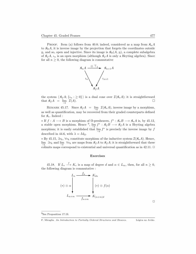
Chapter 45. Graded Frames 477
Proof. Item (a) follows from 40.8; indeed, considered as a map from KnAto KNA, it is inverse image by the projection that forgets the coordinates outsiden, and so, open and injective. Since its image is KN(A, n), a complete subalgebraof KfA, ιn is an open morphism (although KfA is only a Heyting algebra). Sincefor all n ≥ 0, the following diagram is commutative
KnA - Kn+1A
ιn ιn+1
KfA
⊗ >1
AAAAAU
the system 〈KfA; ιn : ≥ 0 〉 is a dual cone over I(K∗A); it is straightforwardthat KfA = lim→ I(A).
Remark 45.17. Since KfA = lim→ I(K∗A), inverse image by a morphism,
as well as quantification, may be recovered from their graded counterparts definedfor K∗. Indeed :
∗ If f : A −→ B is a morphism of Ω-presheaves, f∗ : K∗B −→ K∗A is, by 45.12,a stable open morphism. Hence 9, lim→ f∗ : KfB −→ KfA is a Heyting algebra
morphism; it is easily established that lim→ f∗ is precisely the inverse image by f
described in 44.6, with λ = IdΩ.
∗ By 45.15, ∃vk, ∀vk constitute morphism of the inductive system I(K∗A). Hence,lim→ ∃vk and lim→ ∀vk are maps from KfA to KfA; it is straightforward that these
colimits maps correspond to existential and universal quantification as in 42.11. 2
Exercises
45.18. If L∗f−→ K∗ is a map of degree d and α ∈ Lm, then, for all n ≥ 0,
the following diagram is commutative :
Ln+m
Ln
?
- Kdn
(∗) ⊗ α
fn
K(n+m)d
(∗) ⊗ f(α)
fn+m
?-
2
9See Proposition 17.19.
F. Miraglia. An Introduction to Partially Ordered Structures and Sheaves. Logica no Aviao.

Bibliography
[1] R. Arens and I. Kaplansky. Topological representation of algebras. Trans. Amer. Math. Soc.,63:457–481, 1949.
[2] M. F. Atiyah and I. G. MacDonald. Introduction to Commutative Algebra. Addison-Wesley
Publ. Co., Reading, Massachussetts, 1969.[3] R. Balbes and Ph. Dwinger. Distributive Lattices. Univ. of Missouri Press, Columbia, Mis-
souri, 1974.
[4] H. Bass. Algebraic K-Theory. W. A. Benjamin, New York, 1968.[5] G. Birkhoff. Lattice Theory. AMS Colloquium Publications, Providence, Rhode Island, third
edition, 1967.
[6] A. B. Carson. Model Completions, Ring Representations and the Topology of the Piercesheaf, volume 209 of Pitman Research Notes. Longman Scientific and Tecnical, Essex, UK,
1989.[7] C. C. Chang and H. J. Keisler. Model Theory. North Holland Publ. Co., Amsterdam, 1990.
[8] R. Cignoli. A Hahn-Banach Theorem for Distributive Lattices. Revista da Union Matematica
Argentina, 25:335–342, 1971.[9] W.W. Comfort and S. Negrepontis. Chain Conditions in Topology, volume 79 of Cambridge
Tracts in Mathematics. Cambridge Univ. Press, Cambridge, UK, 1982.
[10] M. Dickmann and F. Miraglia. Special Groups : Boolean theoretic methods in the theory ofquadratic forms, volume 654 of Memoirs of the AMS. American Math. Society, Providence,
RI, 2000.
[11] D. P. Ellerman. Sheaves of Structures and Generalized Ultraproducts. Annals of Pure andApplied Logic, 7:165–195, 1974.
[12] R. Engelking. General Topology, volume 6 of Sigma Series in Pure Mathematics. Helderman
Verlag, Berlin, (revised and completed edition), 1989.[13] R. Engelking and A. Pelczynscki. Remarks on dyadic spaces. Colloquium Math., 11:55 – 63,
1963.[14] S. Feferman and R. Vaught. First Order Properties of Products of Algebraic Systems. Fund.
Math., 47:57 – 103, 1959.
[15] M. Fourman and D. S. Scott. Sheaves and Logic. In D.S.Scott M.Fourman, C.J.Mulvey,editor, Applications of Sheaves, volume 753 of Lecture Notes in Mathematics, pages 302 –
401. Springer-Verlag, Berlin, 1979.[16] D. H. Fremlin. Topological Riecz Spaces and Measure Theory. Cambridge University Press,
1974.
[17] G. Gierz et alia. A Compendium of Continuous Lattices. Springer Verlag, Berlin, 1980.
[18] D. Gluschankof and M. Tilli. On Some Extension Theorems in Functional Analysis and theTheory of Boolean Algebras. Prepublications de l’Equipe de Logique Mathematique, 1990.
[19] R. Godement. Topologie Algebrique et Theorie des Faisceaux. Hermann, Paris, 1958.[20] J. K. Goldhaber and G. Ehrlich. Algebra. The Macmillan Co., New York, 1970.[21] G. Gratzer. General Lattice Theory. Academic Press, New York, 1978.
[22] H. Grauert and R. Remmert. Coherent Analytic Sheaves, volume 265 of Grundlehren derMath. Wissen. Springer-Verlag, Berlin, 1984.
478
Bibliography 479
[23] M. J. Greenberg and J. R. Harper. Algebraic Topology : a first course. Benjamim/Cummings
Publ. Co., Reading, Mass., 1981.
[24] A. Grothendieck and J. Dieudonne. Elements de Geometrie Algebrique I, volume 166 of
Grunlehren der Math. Wissen. Springer-Verlag, Heidelberg, 1971.
[25] R. Hartshorne. Algebraic Geometry, volume 52 of Graduate Texts in Mathematics. Springer-Verlag, New York, 1977.
[26] D. Higgs. The Theory of Omega-sets. mimeographed notes, 1984.
[27] G. P. Hochshild. Basic Theory of Algebraic Groups and Lie Algebras, volume 75 of GraduateText in Mathematics. Springer-Verlag, S. Francisco, 1997.
[28] M. Hochster. Prime Ideal Structure in Commutative Rings. Trans. Amer. Math. Soc.,142:43–60, 1969.
[29] K. H. Hofmann. Representations of Algebras by Continuous Sections. Bull. Amer. Math.
Soc., 78:291–373, 1972.[30] D. Husemoller. Fiber Bundles, volume 20 of Graduate Text in Mathemetics. Springer-Verlag,
Berlin, 1966.
[31] J. R. Isbell. Atomless Parts of Spaces. Math. Scand., 31:5 – 32, 1972.[32] B. Iversen. Cohomology of Sheaves. Springer-Verlag, Berlin, 1986.
[33] N. Jacobson. Basic Algebra I, II. W. H. Freeman Co., New York, 1980.
[34] P. T. Johnstone. Stone Spaces, volume 3 of Cambridge Studies in Advanced Math. Cam-bridge Univ. Press, Cambridge, 1983.
[35] G. Kalmbach. Orthomodular Lattices. Academic Press, N. York, 1983.
[36] I. Kaplansky. Topological representation of algebras II. Trans. Amer. Math. Soc., 63:62–75,1950.
[37] M. Kashiwara and P. Schapira. Sheaves on Manifolds, volume 292 of Grund. der Math.Wissen. Springer-Verlag, Berlin, N. York, 1994.
[38] S. C. Kleene. Introduction to Metamathematics. North Holland Publ. Co., Amsterdam, 1952.
[39] S. C. Kleene. Mathematical Logic. John Wiley and Sons, Inc., New York, 1967.[40] K. Kunen. Set Theory : An Introduction to Independence Proofs, volume 102 of Studies in
Logic. North Holland Publ. Co., Amsterdam, 1980.
[41] S. Lang. Algebraic Number Theory. Addison-Wesley Publ. Co., Reading, Mass, 1970.[42] W. A. J. Luxemburg and A. C. Zaanen. Riecz Spaces, volume 1. North Holland Publ. Co.,
Amsterdam, 1971.
[43] A. Macintyre and J. G. Rosenstein. ℵ0-Categoricity for Rings without Nilpotents Elementsand for Boolean Structures. Journal of Algebra, 43:129–154, 1976.
[44] S. MacLane. Categories for the Working Mathematician. Springer-Verlag, New York, 1971.
[45] S. MacLane. Homology. Springer-Verlag, Berlin, 1987.[46] A. R. Magid. The Separable Galois Theory of Commutative Rings, volume 27 of Pure and
Applied Mathematics Series. Marcel Dekker, Inc., New York, 1974.
[47] W. S. Massey. Algebraic Topology : an introduction. Hartcourt, Brace and World, N. York,1967.
[48] J. Milnor. Introduction to Algebraic K-theory, volume 72 of Annals of Math. Studies. Prince-ton University Press, Princeton, N. J., 1971.
[49] F. Miraglia. On ℵ0-Categorical Biregular Rings. PhD thesis, Yale University, 1977.
[50] F. Miraglia. The Downward Lowenheim-Skolem Theorem for l-structures in Ω-sets. Con-temporary Mathematics, 69:189–208, 1988.
[51] F. Miraglia. Teoria dos Conjuntos : um mınimo. Editora da Universidade de Sao Paulo,1992.
[52] F. Miraglia and U. Solitro. Sheaves over Right-Sided Idempotent Quantales. Logic Journalof the IGPL, 6:545–600, 1998.
[53] B. Mitchell. Theory of Categories. Academic Press, New York, 1965.[54] J. D. Monk and R. Bonnet, editors. Handbook of Boolean Algebras, volume 1, 2 and 3.
North-Holland Publ. Co., Amsterdam, 1989.[55] C. Mulvey. Intuitionistic Algebra and the Representation of Rings. Memoirs of the AMS,
148:3–57, 1974.
F. Miraglia. An Introduction to Partially Ordered Structures and Sheaves. Logica no Aviao.
Bibliography 480
[56] D. B. Mumford. Abelian Varieties. Oxford Univ. Press, Oxford, UK, 1970.
[57] R. S. Pierce. Modules over Commutative Regular Rings, volume 70 of Memoirs of the AMS.American Math. Society, Providence, RI, 1967.
[58] D. Prawitz. Natural Deduction. A proof-theoretical study. Almquist and Wiksell, Stockholm,
1965.[59] H. Rasiowa. An Algebraic Approach to Non-Classical Logics. North Holland Publ. Co. and
PWN-Polish Scientific Publ., Amsterdam and Warsaw, 1974.
[60] H. Rasiowa and R. Sikorski. The Mathematics of Metamathematics, volume 41. Polish Acad-emy of Science Publications, Warsaw, second edition, 1968.
[61] K. I. Rosenthal. Quantales and their Applications, volume 234 of Pitman Research Notes
in Math. Longman Scientific & Tecnical, Essex, UK, 1990.[62] H. Rubin and J. E. Rubin. Equivalents of the Axiom of Choice. North-Holland Publ. Co.,
Amsterdam, 1963.
[63] H. Schaeffer. Topological Vector Spaces, volume 3 of Graduate Text In Math. Springer–Verlag, N. York, third edition, 1970.
[64] H. Schaeffer. Banach Lattices and Positive Operators. Springer-Verlag, Berlin, 1974.[65] D. S. Scott. Identity and Existence in Intuitionistic Logic. In D.S.Scott M.Fourman,
C.J.Mulvey, editor, Applications of Sheaves, volume 753 of Lecture Notes in Mathematics,
pages 660 – 696. Springer-Verlag, Berlin, 1979.[66] J. P. Serre. Faisceaux Algebrique Coherents. Annals of Math., 61:197–278, 1955.
[67] I. R. Shafarevich. Basic Algebraic Geometry, volume 213 of Grundlehren der Math. Wissen.
Springer-Verlag, Heidelberg, 1974.[68] J. R. Shoenfield. Mathematical Logic. Addison-Wesley Publ. Co., Reading, Mass., 1967.
[69] R. Sikorski. Boolean Algebras. Springer Verlag, Berlin, third edition, 1969.
[70] H. Simmons. A Framework for Topology. In Logic Colloquium 1977. North-Holland Publ.Co., 1978.
[71] R. M. Smullyan. First-Order Logic. Springer-Verlag, N. York, 1968.
[72] R. M. Solovay. A New Proof of a Theorem of Gaifman and Hales. Bull. Amer. Math. Soc.,72:282 – 284, 1966.
[73] V. Srinivas. Algebraic K-Theory, volume 90 of Progress in Math. Birkhauser, Boston, Mass.,1996.
[74] Richard G. Swan. Algebraic K-Theory, volume 76 of Lecture Notes in Math. Springer Verlag,
Berlin, 1968.[75] B. R. Tennison. Sheaf Theory, volume 20 of London Math. Soc. Lecture Notes. Cambridge
University Press, 1975.
[76] H. Volger. The Feferman-Vaught theorem revisited. Colloquium Mathematicum, 36:1–11,1976.
[77] A. Wilansky. Topology for Analysis. Ginn and Waltham, Massachusetts, 1970.
[78] A. C. Zaanen. Riesz Spaces, volume 1 and 2. North Holland Publ. Co., Amsterdam, 1981.
F. Miraglia. An Introduction to Partially Ordered Structures and Sheaves. Logica no Aviao.
Index
2Xλ , 30
B(T ), 19
Bλ(X), 30
Fin(B), 15
R pf | Jq , 440
Rad(R), 96
Reg(T ), 19
S(L), 178
Sent(L), 159
Spec(R), 178
U(R), 99
C(X), 21
C(X,Y ), 21
Λ(X), 184
⊥⊥⊥I , 410
>>>I , 410
PP (X), 251, 258
∃vi, 451
∀vi, 451
PP (X), 252, 258
a pc | Jq , 438
fv, 463
pFκ(X,Y ), 30
pFω(X,Y ), 30
σ(S), 101
σ(a), 102
`C , 160
cF(L), 132
cI(L), 132
nzd(R), 99
opA, 463
op(A,K), 463
op(A,n), 463
pS, 397
S←, 28
f∗A, 346, 365
A∗, 30
βX, 204
H, 159
I(L∗), 470
S→, 28
a←, 26
∃πJS, 446
∀πJS, 446
KIA, 400
KfA, 463
KnA, 400
K0A, 401, 402
η∗, 180
O, 470
P(A), 398
kr, 386
NN, 171
`H, 160
2X , 30
f|S , 15√S, 97
RP , 109
ZT , 99
Za, 99
[x ≡ y], 328
εhA, 341
∃f , 442
∀f , 442
P>(A), 394
dhA, 358
ihB, 365
skA, 329
⊆f , 15
chA, 343, 344, 358
a→, 26
, 40
g pf | Jq , 440
accumulation point, 205
adjoint pair, 83
adjointness theorem
for graded direct image, 475
481

Index 482
for graded inverse image, 475
algebra, 42
A-, 145
σ-, 177
algebraic
element of a poset, 40
poset, 40
associated poset, 27
atom, 29
base space, 218
basis
for a space, 18
in complete lattice, 80
Boolean algebra, 63
of regular elements, 79
Booleanization
of a topological space, 193
bounded, 28
above, 28
below, 28
bundle
A-, 145
card(A), 15
cardinal of a set, 15
categorical constructions
in Sh(Ω), 325
category, 143
Cartesian closed, 268
cocomplete, 153
complete, 153
dual, 144
equivalent, 150
finitely complete, 153
locally small, 145
of graded frames, 471
product of, 145
set-based, 143
small, 143
with zero, 145
cHa, 86
chain, 32
in a poset, 32
characteristic map, 400
image by a Q-morphism, 419
inverse image by a Q-morphism, 419
of a subset of |A|I , 406
representation theorem, 407
clopen, 19
in a distributive lattice, 63
closed, 17
in a Ω-set, 394
map, 21
representation of P> by characteristic
maps, 407
closure, 252
in a Ω-set, 394
of a set, 18
cobasis, 91
coequalizer, 153
in pSh(X), 264
in Sh(Ω), 325
in Sh(X), 265
of lattice morphisms, 49
cofinal, 35
down (dcof), 35
up (ucof), 35
cokernel
of a morphism, 54
colimit
for morphisms of I-diagrams, 166
in a category, 152
in L-mod, 165
compact
element of a poset, 40
in a topological space, 22
poset, 40
relatively, 22
compatible, 222, 293, 299
for partial maps, 16
in a presheaf, 237
over p, 294, 299
restriction and equality, 301
complement, 63
of a set, 15
complemented, 63
complete
Ω-set, 311
Boolean algebra
graded, 468
pseudo Boolean algebras, 86
complete Heyting algebra, 86
completeness
for L-mod, 162
completion
along a semilattice morphism, 343
functor, 318
geometrical, 384
of a Ω-set, 315
of a H-set, 346
of a Boolean algebra, 135
of a Heyting algebra, 135
of a presheaf along a semilatticemorphism, 358
of a presheaf over a topological space,257
preservation of finite products, 324
F. Miraglia. An Introduction to Partially Ordered Structures and Sheaves. Logica no Aviao.

Index 483
composition
of characteristic maps, 438
of graded frame morphisms, 471
of relations, 263
cone, 151
dual, 152
congruence
frame, 116
frame (generated by a set), 117
generated by a filter, 54
generated by a morphism, 47
generated by an ideal, 54
constant presheaf, 300
continuous, 21
conucleus, 130
convergence
filter-, 205
of a map along a filter, 205
coproduct
empty, 291
in Sh(Ω), 325
in a category, 153
of lattice morphisms, 46
of lattices, 45
of presheaves, 249
of sets, 17
coreflection, 150
coreflective subcategory, 150
coretraction, 145
degree
component of – n, 467
of a map of graded frames, 470
of an element, 467
dense, 77, 222
ρ-, 309
in a Ω-set, 297
in a presheaf, 252
in another element, 77
restriction, 310
set, 19
density, 21
of a Ω-set, 297
dependence on coordinates
for characteristic map, 430
for closed subpresheaves of AI , 430
for morphisms of Ω-sets, 430
for presheaves over X, 261
diagonal of Pn, 282
diagram in a category, 150
difference of sets, 15
directed
down (dd), 35
left, 35
right, 35
up (ud), 35
discrete sheaf, 238
discrete topology, 17
disjoint union of sets, 17
domain
of a L-set, 285
of a presheaf, 235
dual cone, 152
duality, 150
embedding
L-, 161
elementary, 161
of posets, 26
regular, 81
enough injectives, 155
enough projectives, 154
epimorphism, 145
equality
in a L-set, 285
in a geometric sheaf, 220
in a presheaf, 236
strict, 328
equalizer, 153, 291
in Sh(Ω), 325
of presheaf morphisms, 248
equivalence
class, 16
in a Heyting algebra, 74
of categories, 150
relation, 16, 263
generated in a presheaf, 263
on a L-set, 457
essential image
of a presheaf, 356, 357
exchange rules, 298
existential quantification
for presheaves, 262
extension
as adjoint to restriction, 353
essential (for closed sets), 192
of a presheaf, 350, 352
extension theorem
for BA-morphism, 140
extensional, 236
L-set, 285
extensionalization, 242
functor, 342
extent
of a characteristic map, 400
in a presheaf, 299
of a section, 235
of a section in a L-set, 285
F. Miraglia. An Introduction to Partially Ordered Structures and Sheaves. Logica no Aviao.

Index 484
of a singleton, 315
exterior power, 411
empty, 411
exterior product, 411
Feferman-Vaught value
of a formula, 271
fiber
at a filter, 374
fibered product, 153, 290
in Sh(Ω), 325
of L-presheaves, 305
of bundles over a base space, 228
of geometric presheaves, 248
of lattices, 45
over a morphism, 228
over a sheaf morphism, 232
filter∨-, 112∧-, 115
base, 35
complete, 132
generated by, 132
completely prime, 120
generated by S in a lattice, 49
in 2X , 35
in a poset, 35
irreducible, 61
lattice, 49
maximal, 59
prime, 59
principal, 35
proper, 35
filtered power, 275
bounded, 276
filtration, 275
final object, 145
for presheaves, 247
in Sh(Ω), 325
finitary
operations, 463
relations, 463
finite intersection property, 49
finite union property, 49
finitely complete
L-set, 297
presheaf, 271
fixed point theorem, 81
fixing coordinates
in a characteristic map, 410
flabby, 238, 310
locally, 326
formula, 158
∀∃, 159
existential, 159
Horn, 159
positive, 159
primitive, 159
quantifier-free, 159
universal, 159
frame, 85
free, 137
with enough points, 121
free
algebra, 135, 136
frame, 137
frontier of a set, 18
functor, 145
s -, 331
bi-, 147
change of base, 342
complete extension, 354
faithful, 146
forgetful, 146
full, 146
morphism, 147
preserves colimits, 153
preserves limits, 153
regularization, 386
representable, 148
Stone space, 180
Zariski spectrum, 180
fundamental theorem
for lattice morphisms, 47
for quotient by ideals, 55
for quotients by filters, 55
Gaussian domain, 104
generic point, 122
germ of a section, 374, 377
Gleason cover, 212
global section
of a L-set, 285
gluing
in a Ω-set, 296
of a subset, 299
gluing lemma
for pF (X,Y ), 16
graded
cBa, 468
frame, 467
greatest lower bound, 28
Heyting algebra (HA), 71
homeomorphism, 21
local, 217
ideal
F. Miraglia. An Introduction to Partially Ordered Structures and Sheaves. Logica no Aviao.
Index 485
base, 35
complete, 132
generated by a set, 132
generated by S in a commutative ring,94
generated by S in a lattice, 49
in 2X , 35
in a commutative ring, 94
in a poset, 35
lattice, 49
maximal, 59
prime, 59
in a commutative ring, 95
principal, 35
product
in a commutative ring, 94
proper, 35
radical
in a commutative ring, 96
sum
in a commutative ring, 94
idempotent, 186
image
as a graded map on K∗, 474
by a Ω-set morphism, 398
by a morphism in pSh, 423
by a Q-morphism, 419
of a L-set along a semilattice morphism,341
of a presheaf along a semilattice
morphism, 358
of a sheaf along a continuous map, 365
of a sheaf along a semilattice morphism,344
implication
for closed subpresheaves, 258
for subpresheaves, 258
in a Heyting algebra, 71
inductive
limit, 153
system, 151
infimum (inf), 28
initial object, 145
for presheaves, 247
in Sh(Ω), 325
injective
Boolean algebra, 141
hull, 155
in a category, 155
interior of a set, 18
inverse image
as a graded map on K∗, 474
by a Ω-set morphism, 398
by a morphism in pSh(X), 260
by a morphism in pSh, 423
by a Q-morphism, 419
of a presheaf along a semilatticemorphism, 365
of a sheaf along a continuous map, 346
invertible element, 99
irreducible, 122
isomorphism, 145
join, 28, 44
in PP (X), 256
kernel
of a morphism, 54
of a presheaf morphism, 264
of a sheaf morphism, 228
Kripke models, 85
lattice, 44
[∨,∧
]-, 86
[∧,∨
]-, 86
complete, 80
distributive, 52
zero-dimensional, 90
least upper bound, 28
left adjoint, 83
Lemma
gluing, 16
Yoneda’s, 148
Zorn’s, 32
limit
along a filter, 205
for morphisms of I-diagrams, 165
in a category, 152
in L-mod, 162
inductive, 153
of a map along a filter, 205
projective, 153
linear element, 90
linear order, 32
local homeomorphism, 217
localization
at D, 426, 454
of a L-set at a filter, 374
of a ring at a prime ideal, 109
lower bound, 28
lower set, 29
map
I-characteristic, 400
n-characteristic, 400
closed, 21
continuous, 21
essential, 211
minimal, 211
F. Miraglia. An Introduction to Partially Ordered Structures and Sheaves. Logica no Aviao.

Index 486
of graded frames, 470
of graded frames over Ω, 470
open, 21
spectral, 185
maximal, 29
maximum, 28
meet, 28, 44
minimal, 29
minimum, 28
modular law, 52
Modus Ponens, 72, 160
monomorphism, 145
morphism
[∨
,∧
]-, 81
[∧,∨
]-, 81∨-, 80∧-, 80
L-, 161
characteristic, 267
complete, 81
cone-, 152
epic, 145
epic (for presheaves), 249
evaluation, 268
fiber – at a filter, 374
frame, 85
implication preserving (ip), 87
from L-set to a P -set, 334
HA-, 71
image of a, 259
increasing, 26
lattice, 44
localization, 374
monic, 145
monic (for presheaves), 249
of I(L∗), 470
of I-diagrams, 164
of L-sets, 288
of geometric sheaves, 218
of graded frames, 470
of pre-ordered sets, 26
of presheaves, 234
of presheaves over distinct topologicalspaces, 336
of sheaves, 237
open, 87
restriction of a, 259
stable, 470
stalk, 377
multiplicative subset, 95
natural equivalence, 148
natural number object, 278
natural transformation, 148
negation
for closed subpresheaves, 258
for subpresheaves, 258
neighborhood of a point, 18
nucleus, 126
open, 17
map, 21
operator
idempotent, 126
implicative, 126
order
lexicographic, 32
linear, 32
opposite, 28
partial, 26
pre-, 26
reverse, 28
total, 32
well-ordering, 32
orthomodular law, 52
partial order (po), 26
extension, 30
partition
of a measure space, 31
of a set, 31
point
generic, 122
in a complete lattice, 120
poset, 26
algebraic, 40
compact, 40
continuous, 40
predicate calculus
classical, 160
intuitionistic, 159
presheaf
of C-objects, 234
as a Ω(X)-set, 285
extensionalization of a, 242
finitely complete, 271
flabby, 310
over a semilattice, 299
extensional, 299
restriction in, 234, 235
section of a, 234
pro-constructible set, 197
product
empty, 289
in Sh(Ω), 325
in a category, 153
of L-sets, 289
of L-structures, 162
F. Miraglia. An Introduction to Partially Ordered Structures and Sheaves. Logica no Aviao.
Index 487
of lattices, 45
of maps, 16
of posets, 31
of presheaves, 248
of sets, 16
of sheaves, 248
reduced, 56
topology, 23
projection, 126
projective
cover, 154
in a category, 154
limit, 153
system, 151
proof, 160
proper
multiplicative set, 95
pseudo-complement, 72
pullback, 153
pushout, 153
Q-morphism, 414
Q-operator, 126
quantifier
as a morphism on I(K∗A), 476
classical, 445, 446, 451
existential, 261
along f , 442
universal, 261
along f , 442
quotient
L-structure, 168
distributive lattice, 53
for presheaves, 264
for sheaves, 265
lattice, 47
of a L-presheaf, 458
of a L-set, 458
of a sheaf, 458
ring, 179
reduced product, 56
refinement
of partitions, 31
reflection, 150
reflective subcategory, 150
regular, 77
closed set, 19
monic, 292
open set, 19
ring, 186
regularization
associated to double negation, 389
by double negation, 428, 454
relation
in pSh(X), 262
inverse of a, 456
on a Ω-presheaf, 456
on presheaves, 456
representation theorem, 407
restriction
as adjoint to extension, 353
in a geometric sheaf, 219
in a presheaf, 299
of a characteristic map, 401
of a L-set to p, 286
of a map, 15
of a presheaf to p, 301
of a presheaf to a subsemilattice, 301
of a presheaf to an open set, 238
restriction dense, 310
retract, 337
retraction, 145
right adjoint, 83
ring
Noetherian, 105
of fractions, 106
total, 111
von Neumann regular, 186
zero, 107
saturated, 99
saturation, 101–103
section
continuous, 219
extent of a, 219
global, 219, 299
of a L-set, 285
of a map, 217
of a presheaf, 299
semicontinuous
lower, 31
upper, 31
semilattice, 44
[∧,∨
]-, 295
join, 44
sentence, 159
separation
by a family of functions, 22
by a family of subsets, 21
sequence, 281
set
Ω-
associated to a presheaf, 302
complete, 311
constant, 288
L-, 285
bounded constant, 287
F. Miraglia. An Introduction to Partially Ordered Structures and Sheaves. Logica no Aviao.

Index 488
irreducible, 122
pro-constructible, 197
sheaf, 237
constant geometric, 221
discrete, 238
domain of a, 219
geometrical, 218
Hausdorff geometric, 227
of closed subpresheaves, 398
of continuous functions, 239
of morphisms, 268
of opens, 238
of subsheaves, 265, 266, 398
over Ω, 311
sections of, 219
skyscraper, 373
sheaf representation
of a commutative ring, 321, 324
of a Heyting algebra, 224, 232
of a regular ring, 226, 233
of an integral domain, 225, 233
sheaf space, 218
sheafification, 257
singleton, 315
skyscraper sheaf, 373
solution sets, 154
soundness
of Intuitionistic Propositional Calculus
in KfA, 466
space
Baire, 171, 197
base, 218
Boolean, 170
Cantor, 170
compact, 22
completely regular, 22
completely spectral, 204
connected, 189
covering, 221
dyadic, 171
extremally disconnected, 204
Hausdorff or T2, 22
Lindeloff, 21
locally compact, 42
normal or T4, 22
regular or T3, 22
second countable, 21
separable, 21
sheaf, 218
sober, 121
spectral, 190
Stone, 178
T0, 22
T1, 22
topological, 17
totally disconnected, 170
specialization po, 30
spectrum
of a commutative ring, 95, 178
stable morphism, 470
stalk, 377
of a geometric sheaf, 218
Stone duality, 192
Stone space, 178
Stone-Cech compactification, 157, 206
structure, L-, 161
sub-basis
for a space, 18
sub-Boolean algebra
generated by a set, 139
subbasis
in a complete lattice, 80
subcategory, 143
full, 143
subframe, 85
sublattice, 44
regular, 81
subobject
classifier, 267
in a category, 145
subpresheaf, 251
closed, 252
closed – generated by, 252
generated by, 252
subsheaf, 251
characteristic, 267
substitution
in a sequence, 404
of a J-sequence in a I-sequence, 438
of a term for a variable, 159
of morphisms in R ∈ K1(AI), 441
of morphisms in R ∈ KIA, 440
of morphisms into a morphism, 440
support
of a presheaf, 236
of a product, 305
of a set of sections
in a L-presheaf, 299
in a L-set, 285
of an exterior power, 412
of powers, 290
of products, 290, 305
supremum (sup), 28
symmetric difference
of sets, 15
tensor product
of characteristic maps, 471
F. Miraglia. An Introduction to Partially Ordered Structures and Sheaves. Logica no Aviao.
Index 489
term, 158
free for a variable, 159theorem, 160
adjoint functor-, 154
Feferman-Vaught, 272representable functor-, 154
Stone’s, 192
Stone-Weierstrass, 176Tychonoff’s, 24
Urysohn separation, 22
theory, 160topology, 17
constructible, 197
discrete, 17finer than, 17
generated, 17induced, 17
product, 23
Stone, 180subspace, 17
Zariski, 180
total order, 32total ring of fractions, 111
tree, 32
Y -branching, 33binary, 34
ultrafilter, 59ultraproduct, 59
unit, 99
upper bound, 28upper set, 29
variablebound, 159
free, 159
in a finitary operation, 463in a finitary relation, 463
way below, 40weight, 21
well-founded, 32well-ordering, 32Well-Ordering Axiom (WOA), 33
Yoneda’s Lemma, 148
zero
-divisor, 99
in a category, 145ring, 107
Zorn’s Lemma, 32
F. Miraglia. An Introduction to Partially Ordered Structures and Sheaves. Logica no Aviao.

I.S.B.N. 978-65-00-06148-2