lexicographic local search and the p-center problem

European Journal of Operational Research 151 (2003) 265–279

www.elsevier.com/locate/dsw

Lexicographic local search and the p-center problem

Refael Hassin, Asaf Levin *, Dana Morad

Department of Statistics and Operations Research, School of Mathematical Sciences, Tel-Aviv University, Tel-Aviv 69978, Israel

Abstract

We introduce a local search strategy that suits combinatorial optimization problems with a min–max (or max–min)

objective. According to this approach, solutions are compared lexicographically rather then by their worst coordinate.

We apply this approach to the p-center problem.

� 2003 Elsevier B.V. All rights reserved.

Keywords: Facility planning; Heuristics

1. Introduction

The subject of this paper is the application of

local search to the class of bottleneck problems. In

these problems, each feasible solution, say X , isassociated with a vector, say cX 2 Rn, and the goal

is to minimize maxi cXi (or maximize mini cXi ). Forexample, Hochbaum and Shmoys [11] considered a

class of problems in which a weighted graph is

given and we wish to find a subgraph satisfying

some requirements such that the length of the

longest edge included in the subgraph is mini-

mized. Several problems from this class emerging

from routing, location, and communication net-

work design, are described there in detail.We observe that bottleneck problems are quite

insensitive to local changes in the solution. This is

in contrast to the case whereP

i cXi is minimized.

We suggest dealing with this drawback by con-

* Corresponding author.

E-mail addresses: [email protected] (R. Hassin), lev-

[email protected] (A. Levin).

0377-2217/$ - see front matter � 2003 Elsevier B.V. All rights reserv

doi:10.1016/S0377-2217(02)00825-1

sidering a more sensitive measure that ranks so-

lutions which have the same objective value. Our

approach is of sorting the elements of the solution

vectors and then comparing them lexicographi-

cally. We call the resulting algorithm lexicographic

local search. This approach can be incorporated in

various local improvement approaches such assimulated annealing and tabu search.

In recent years many heuristic approaches were

designed that include a local search procedure as a

subroutine. Such approaches include for example

simulating annealing and tabu search. We suggest

to incorporate the proposed lexicographic local

search in such heuristics when solving a bottleneck

problem. We demonstrate the power of using lex-icographic local search in such circumstances by

using it in simulating annealing.

Our goal in this paper is to examine the effect of

modifying a local search heuristic by the use of

lexicographic local search.

We discuss lexicographic local search in the

context of the p-center problem. We present some

theoretical results which motivate our use of lexi-cographic local search and show the limitation of

ed.

mail to: [email protected]

266 R. Hassin et al. / European Journal of Operational Research 151 (2003) 265–279

this approach. Then we concentrate on a compu-

tational study. Our results indicate that lexico-

graphic local search is a useful tool. It improves

(with respect to local search) the quality of the

solutions without increasing the computationaleffort. In many cases we were able to receive a

higher frequency of the best solution using lexi-

cographic local search. This higher frequency

means that if we were running the algorithms for a

shorter time period the chances of getting the

better result would be higher.

An interesting bottleneck problem is that of

minimizing the maximum completion time whenscheduling jobs on m parallel machines. Here a

solution is associated with an m-vector giving the

completion time on each machine. Glass et al. [7]

applied local search to this problem. They defined

as an improvement a step that either decreases the

maximum completion time or keeps it unchanged

but decreases the number of machines that achieve

it. Lexicographic search can be considered as afurther step towards improving the sensitivity of

the search to promising directions by considering

not only the number of occurrences of the maxi-

mum completion time but also the next highest

completion times.

F€uurer and Raghavachari [5] developed an ap-

proximation algorithm for minimizing the maxi-

mum node degree of a spanning tree. The localsearch they developed swaps pairs of edges when

the maximum degree of the four nodes involved is

reduced, even when this does not affect the maxi-

mum degree of the tree. A different variation ap-

pears in [6]. This approach can be viewed as a

variation of lexicographic local search.

Finally, Khanna et al. [12] developed a general

paradigm, non-oblivious local search, in which localoptimality is defined according to a function which

does not just rank solutions that are identical with

respect to the original function, as we do, but in

fact ranks solutions in a different way from that

dictated by the original function. They demon-

strate that a clever choice of this function may

improve the theoretical approximation ratio.

In the next sections we provide a brief descrip-tion of several algorithms for the p-center problemincluding the lexicographic local search. We then

present a worst-case analysis for the p-center

problem of the lexicographic local search and the

other algorithms and we finally present results of a

computational study for the p-center problem and

conclusions we draw from it.

2. The p-center problem

In the p-center problem, a finite set V is given

with a non-negative distance matrix d ¼ dij; i;j 2 V . For a subset X � V , let DiX ¼ minj2X dij bethe distance of i 2 V from the subset X . The

problem is to find X � V such that jX j ¼ p andF ðX Þ ¼ maxv2V DvX is minimized. We call F ðX Þ theradius of X . In an illustrative description of the

problem, V is a set of customers to be served by pservice centers. The goal is to locate the centers so

that the maximum travel time of a customer to the

nearest center is minimized.

The p-center problem is NP-hard even when Vis a set of points in the two dimensional plane andd describes the Euclidean distances among the

points [4]. Assuming that the distance matrix is

symmetric and obeys the triangle inequality, the

polynomial algorithms of Dyer and Frieze [3],

Hochbaum and Shmoys [10] and Plesn�ıık [13] are

fast and guarantee an approximation which is

bounded by twice the optimal solution�s value.

These algorithms are designed to achieve the errorbound and will often produce solutions with an

error that cannot be accepted for practical com-

putations. There are other algorithms that usually

perform well while theoretically their running time

may not be polynomially bounded and the solu-

tions they provide cannot be bounded in the worst

case by any constant. An important example is an

algorithm of Drezner [2] (Cooper [1] used earlier asimilar method for related problems).

3. Local search

The local search approach assumes that for

each solution, X , a neighborhood, NX , is defined.

Then, in each iteration the neighborhood is sear-ched for an improved solution. A natural defini-

tion of a neighborhood in the p-center problem is

the set of solutions obtained by relocating at most

R. Hassin et al. / European Journal of Operational Research 151 (2003) 265–279 267

k centers of the current solution, for some pre-

specified k. In our study we assume k ¼ 1.

Algorithm LS:

1. Start with an arbitrary solution X . (This may be

the output of some other heuristic.)

2. Let NX be the set of solutions obtained from Xby relocating a single center. Scan NX for a bet-ter solution, X 0. If none exists, stop and output

X . Else, replace X by X 0 and repeat.

The search terminates in a local optimum, a

solution which is best in its neighborhood. Clearly,

the specific output depends on the choice of the

initial solution, and a common practice is to repeat

the search many times, starting from different ini-tial solutions, and finally select the best outcome.

We note that each iteration of the algorithm

(i.e., reaching a local minimum from a given initial

point) requires polynomial time. The reason is that

the number of improvements is bounded by the

number of distinct distance values which is Oðn2Þ.In many applications d is symmetric and satis-

fies the triangle inequality. In the case of twocenters we can use these properties to prove a

performance guarantee for the algorithm.

Theorem 3.1. If d is symmetric and the triangleinequality is satisfied, then the radius of the 2-centersolution produced by Algorithm LS is at most twicethe size of the radius of an optimal solution. Thisbound is tight.

Proof. Let fx1; x2g be an optimal solution with

radius r. Let S1, S2 be a partition of V such that

dv;xi 6 r; v 2 Si; i ¼ 1; 2. For example, Si may be

the set of customers serviced by the center at xiunder the optimal solution. Then, it follows from

the triangle inequality that any solution fy; zg such

that y 2 S1, z 2 S2 satisfies dvy 6 dv;x1 þ dx1;y 6 2r forv 2 S1, and dvz 6 dv;x2 þ dx2;z 6 2r for v 2 S2. Hence,

the radius of any such solution is at most 2r. Itnow follows that a solution whose radius is strictly

greater than 2r cannot be a local minimum since it

must have its two centers located in the same

subset Si and by relocating a center to the other

subset the radius is improved to a value at most 2r.

Consider now four points on the line with co-

ordinates 0; 1; 2; 4. The 2-center solution is f1; 4gwith radius 1. But the solution f0; 2g is a local

minimum and its radius is 2. This proves that the

bound stated by the proposition is tight. �

For p > 2, the ratio of the approximate solution

to the optimal cannot be bounded by a constant.

This will follow from a stronger claim presented in

the next section.

4. Lexicographic local search

Consider a 2-center example. Six points with

coordinates f0; 10; 19; 21; 30; 40g are located on a

line. Consider the solution X ¼ f19; 21g. To im-

prove it, both of its centers must be moved.

Therefore it is a local minimum with respect to LS.

Note however that by moving one of the centers of

X we can reduce the number of points whose dis-tance from their nearest center is 19. Such a

change, while not reducing the radius, is a good

move towards reducing the radius in a following

step.

This example motivates a modification of the

objective function that will make it more sensitive

to promising changes in the solution.

Consider two vectors x; y 2 Rn. Let x0, y0 be thevectors obtained by permuting x, y respectively, so

that x01 P x02 P � � � P x0n and y 01 P y 02 P � � � P y 0n.We say that x is ‘-lexicographically equal to y if forall k 2 f1; . . . ; ‘g, x0k ¼ y0k. We say that x is ‘-lexi-cographically smaller than y if for some k 2f1; . . . ; ‘g, x0i ¼ y 0i ; i ¼ 1; . . . ; k � 1 and x0k < y0k.

The algorithm which we propose in this paper is

a local search variation that scans the neighbor-hood to find an ‘-lexicographically smaller solu-

tion, where ‘ is a predetermined parameter.

Algorithm ‘LEX:

1. Start with an arbitrary solution X .

2. Scan NX for an ‘-lexicographically smaller solu-

tion, X 0 (first improvement). If none exists, stop

and output X . Else, replace X by X 0 and repeat.

In the p-center problem, we associate with each

solution a vector x 2 Rn, where xi is the distance


between node i and its nearest center in the solu-

tion. We apply the lexicographic local search to

obtain a lexicographic local minimum with respect

to this measure.

We note that for any fixed ‘ value, each itera-tion of the algorithm (reaching an ‘-lexicographiclocal minimum from a given initial point) requires

polynomial time. The reason is that the number of

improvements is OðN ‘Þ, where N is the number of

distinct values in the distance matrix d.Clearly 1LEX is equivalent to LS, and 2LEX is

sufficient to reach the optimal solution in the ex-

ample that opened this section. One could gener-alize this example to justify higher ‘ values. Let

V ¼ V1 [ V2 [ V3 where the subsets are of equal

size. Suppose that the distances between points in

each of the subsets are zero, while between subsets

the distances are of one unit. An optimal solution

for pP 3 locates at least one center in each of the

three subsets and its radius is zero. However, a

solution that locates all the centers within onesubset is ‘LEX optimal for all ‘6 n=3, since by

moving one center to another subset DiX remains

one for all points i in the third subset. We conclude

that the ratio of the ‘LEX solution to the optimal

in the worst case cannot be bounded by a constant.

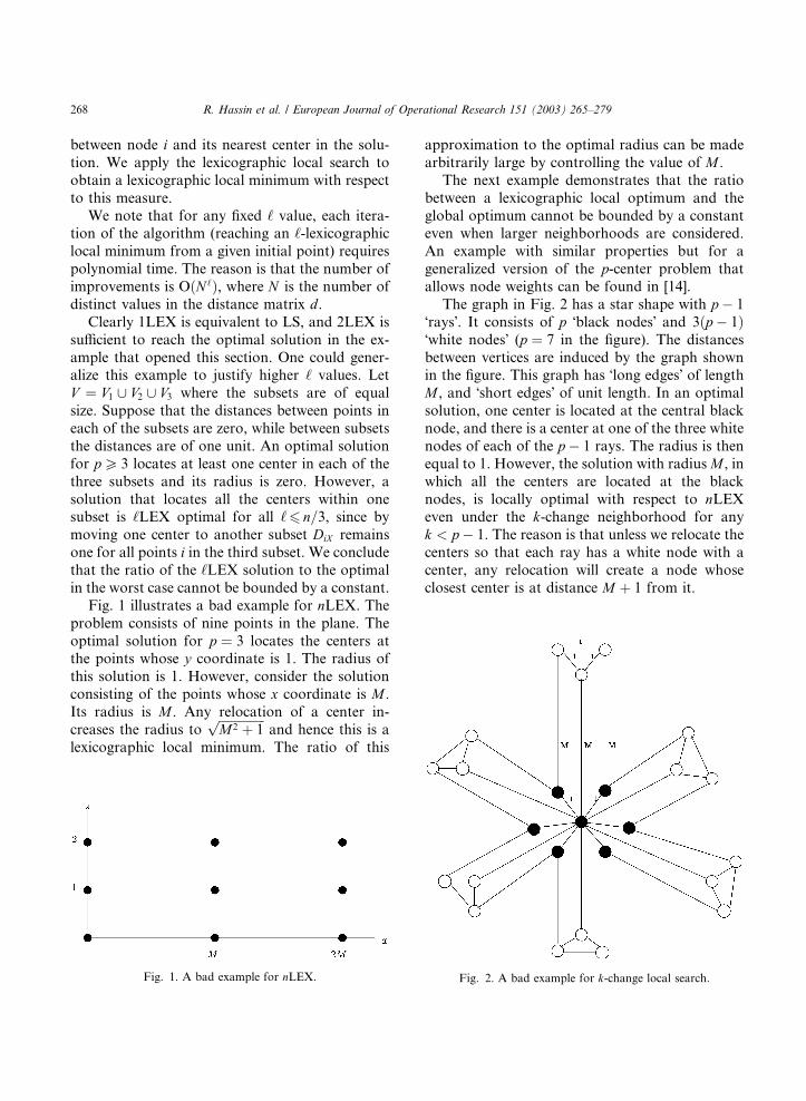
Fig. 1 illustrates a bad example for nLEX. The

problem consists of nine points in the plane. The

optimal solution for p ¼ 3 locates the centers atthe points whose y coordinate is 1. The radius of

this solution is 1. However, consider the solution

consisting of the points whose x coordinate is M .

Its radius is M . Any relocation of a center in-

creases the radius toffiffiffiffiffiffiffiffiffiffiffiffiffiffiffiM2 þ 1

pand hence this is a

lexicographic local minimum. The ratio of this

Fig. 1. A bad example for nLEX.

approximation to the optimal radius can be made

arbitrarily large by controlling the value of M .

The next example demonstrates that the ratio

between a lexicographic local optimum and the

global optimum cannot be bounded by a constanteven when larger neighborhoods are considered.

An example with similar properties but for a

generalized version of the p-center problem that

allows node weights can be found in [14].

The graph in Fig. 2 has a star shape with p � 1

�rays�. It consists of p �black nodes� and 3ðp � 1Þ�white nodes� (p ¼ 7 in the figure). The distances

between vertices are induced by the graph shownin the figure. This graph has �long edges� of lengthM , and �short edges� of unit length. In an optimal

solution, one center is located at the central black

node, and there is a center at one of the three white

nodes of each of the p � 1 rays. The radius is then

equal to 1. However, the solution with radiusM , in

which all the centers are located at the black

nodes, is locally optimal with respect to nLEXeven under the k-change neighborhood for any

k < p � 1. The reason is that unless we relocate the

centers so that each ray has a white node with a

center, any relocation will create a node whose

closest center is at distance M þ 1 from it.

Fig. 2. A bad example for k-change local search.


However, we are able to show that when the

points are distinct points on a line (1-dimension

space) 2LEX provides a 2-approximation algo-

rithm for the 3-center problem whereas LS does

not provide us any constant error ratio as can beseen by the following example:

Let V ¼ f0;M ;M þ 1;M þ 2; 2M þ 2g. The

optimal 3-center is f0;M þ 1; 2M þ 2g with unit

radius. However, fM ;M þ 1;M þ 2g is a local

optimum for LS with radius M .

Theorem 4.1. 2LEX is a 2-approximation algo-rithm for the 3-center problem when all the pointsare distinct points on a line.

Proof. Every solution divides the line into three

segments such that all the points on a segment are

served by the same center. Consider the partition

induced by an optimal solution. Any solution that

locates one center in every segment has a radius of

at most twice the optimal. Consider a 2LEX localoptimum.

If there is one center in each segment it is a

2-approximation.

If there is a segment with two centers and an-

other one with one center, moving one of the two

centers to the third segment will guarantee a 2-

approximation. The algorithm decided not to

move to this solution and therefore, the currentradius is at most twice the optimum.

The remaining case is that there is a segment

with three centers. In order for this solution to

have a radius which is more than twice the opti-

mum, the maximum distance must not be achieved

in the segment of the three centers. If there is only

one point with distance from its nearest center

which is the maximum distance then moving acenter to the segment which contains this point

will reduce the radius. Therefore, there are exactly

two points, a and b, with a distance from their

nearest neighbor which equals the maximum dis-

tance (as all the points are distinct). By moving a

center (the middle center) to another segment (that

contains a) we reach a new solution in which one

of the two maximum distances of the current so-lution is reduced (the distance from a). The dis-

tances which were increased are at most twice the

optimum (these are distances in the segment where

the three centers were located). As the current

solution is a 2LEX local optimum (by assumption)

this case is not possible and the radius is at most

twice the optimal value. �

The bound of the above theorem cannot be

improved as shown by the following example:

Consider the p-center problem on the line with

points f1; 2; 3; 4; 5; 6; . . . ; 3p � 2; 3p � 1; 3pg. The

optimal solution is f2; 5; . . . ; 3p � 1g and it has

radius 1. However, the solution f1; 4; . . . ; 3p � 2gis n-LEX optimal but it has radius 2 (this is so for

pP 2). The distance vector of this solution consistof one entry of 2, 2p � 1 entries of 1 and the rest

are 0. To improve lexicographically one must

change all the centers of the current solution.

The result of Theorem 4.1 cannot be extended

to higher dimension Euclidean spaces and in par-

ticular the graph in Fig. 1 shows that in R2 nLEXdoes not guarantee any constant error ratio when

p ¼ 3.

5. Fast algorithms for the p-center problem

The algorithm of Dyer and Frieze [3] runs in

OðpnÞ time where n ¼ jV j. It is a 2-approximation

for the problem when d satisfies the triangle in-

equality.

Algorithm DF:

1. Locate the first center at an arbitrary pointv 2 V .

2. Given a set of centers X � V . If jX j ¼ p, stopand output X . Else, locate the next center at a

point v 2 V satisfying DvX ¼ maxu2V DuX .

In our computational study, we executed n runs

starting with all possible initial choices. Our

computational study indicates that this imple-mentation is practically useful, however, it does

not improve the error bound of 2 even in the

(polynomially solvable) case of p ¼ 2, as demon-

strated by the following example. Consider six

points on a line with coordinates f1; 2; 3; 4; 5; 6g.Let p ¼ 2. The optimal solution locates the centers

at 2 and 5 and has a radius 1. No matter what is

the initial point, DF will locate the second center


in one of the extreme locations (1 or 6) and the

radius obtained will be 2.

Drezner�s algorithm is a heuristic designed to

practically solve the p-center problem. No poly-

nomial bound on its running time is known and wewill show below that its error ratio cannot be

bounded by a constant. However, it often pro-

duces good solutions in short time. To simplify the

presentation of the algorithm we assume that the

elements of the distance matrix d are all distinct.

Consider a subset X � V . For each j 2 X let

IjðX Þ ¼ fi 2 V jdij ¼ mink2X dikg. Thus, IjðX Þ is theset of customers that will be served by the centerat j, given the solution X .

For j 2 X let kðjÞ be the optimal center�s loca-tion in the 1-center problem in which customers

are located in the subset IjðX Þ and the center can

be located at any point of V . Note that under our

simplifying assumption kðjÞ is unique.

Algorithm DR:

1. Arbitrarily select X � V such that jX j ¼ p.2. If kðjÞ ¼ j 8j 2 X stop and output X . Else, for

each j 2 X such that kðjÞ 6¼ j insert kðjÞ intoX , delete j from X , and repeat this step.

Assuming that the elements of d are distinct, the

algorithm is deterministically determined except

for the choice of the initial solution. One can apply

the algorithm several times, starting with different

initial solutions, and finally select the best of the

solutions that are obtained. Such a strategy is de-sired since otherwise the algorithm may be easily

trapped in bad solutions. For example consider the

graph in Fig. 1 for the 3-center problem (one can

change the distances by infinitesimally quantities

so they all be distinct). If we start with a solution

consisting of the points whose x coordinate is Mthen this solution cannot be improved by DR.

6. The computational study

We compare ‘-lexicographic local search for

‘ ¼ 1; 2; 3; 4 on several p-center instances satisfyingthe triangle inequality. We compare the perfor-

mance of ‘-lexicographic local search with that of

ordinary local search (LS). We produced initial

solutions using various heuristics, and continue

either by LS with neighborhoods allowing a single

relocation of a center, or by simulated annealing

with the same type of neighborhood.

The algorithms were programmed in Fortran 77and ran on Sun4m computers running SunOS 4.1.3

U1. We used different machines for different in-

stances, but all the algorithms that we tested on any

given instance were executed on the same machine.

We tested each instance with several p values.

We applied each algorithm n times, where n is the

number of nodes in the graph. The reason for

executing n runs is that we often used DF to forminitial solutions. DF is deterministic up to the

initial choice and the assumption that the distances

are distinct. In each run we applied DF with a

different starting point.

The detailed test results appear in the appendix.

For each instance and each algorithm, they give

the best solution value obtained in n runs, the

frequency of this value, the average value, theworst value, and the total execution time of the nruns (where s, m, h denote seconds, minutes,

hours, respectively).

The row denoted DF refers to the application of

Dyer and Frieze�s algorithm. DFDR is the com-

bined algorithm that first runs DF and then uses

its output as an initial solution for DR. A DFDR

prefix for LEX means that the lexicographic localsearch started with the output solution obtained

by DFDR.

A SIM prefix means that simulated annealing

was used with the lexicographic criterion (with the

output of DFDR giving the initial solution). To

apply simulated annealing we concatenated each

solution�s ‘ highest elements. For example, when

‘ ¼ 2, a vector ð122; 25; 32; 6Þ will be representedby its two highest elements as 122 032. Applying

LS with this representation is equivalent to ap-

plying 2LEX to the original data. This represen-

tation enabled us to test ‘LEX with different

values of ‘, using the same simulating annealing

code. Since our goal is to test the lexicographic

local search against ordinary local search, the de-

tails of the simulating annealing are not importantand are not described here. Note that it was not

essential to develop an efficient simulated anneal-

ing program.


In our computational study, we changed the

solution whenever a lexicographic improvement

was detected.

On small problems, with up to 50 nodes and

p ¼ 10, the use of lexicographic search was notjustified since the optimal solutions (that were

found separately using an Integer Programming

solver) were also often found by the faster DFDR

algorithm or by LS.

We will present a summary of the results ac-

cording to different criteria. We say that Algo-

rithm A performed better than Algorithm B on a

given instance if the best solution returned by A isbetter than the one returned by B, or the best so-

lutions have the same value but A returned the

best solution more frequently, or if both A and B

returned the same best solution the same num-

ber of times but the average value returned by A

was better. Lastly, A is better than B if both al-

gorithms performed equally with respect to all of

the above mentioned criteria, and A was fasterthan B.

In our study we obtained that DFDR‘LEX is

better than ‘LEX:

• DFDR1LEX had better results on 30 instances

(in 14 instances it produced a better best solu-

tion), whereas 1LEX had better results on six

instances (in one of them it produced a betterbest solution).


(in eight instances it produced a better best so-

lution), whereas 2LEX had better results on

14 instances (in four instances it produced a bet-

ter best solution).


(in three instances it produced a better best so-lution), whereas 3LEX had better results on 15

instances (in four instances it produced a better

best solution).


(in one instance it produced a better best solu-

tion), whereas 4LEX had better results on 17 in-

stances (in one instance it produced a better

best solution).

The following is a summary of the results

comparing ‘LEX to ð‘þ 1ÞLEX:

• 2LEX had better results on 35 instances (in 17

instances it produced a better best solution),

whereas 1LEX had better results on one in-

stance (it never produced a better best result).• 3LEX had better results on 30 instances (in se-

ven instances it produced a better best solution),

whereas 2LEX had better results on four in-

stances (it never produced a better best result).

• 4LEX had better results on 28 instances (in

three instances it produced a better best solu-

tion), whereas 3LEX had better results on six

instances (in one instance it produced a betterbest solution).


comparing DFDR‘LEX to DFDRð‘þ 1ÞLEX:


(in three instances it produced a better best so-

lution), whereas DFDR1LEX had better resultson three instances (it never produced a better

best result).


(in one instance it produced a better best solu-

tion), whereas DFDR2LEX had better results

on 9 instances (it never produced a better best

result).

• DFDR4LEX had better results on 21 instances(in one instance it produced a better best solu-

tion), whereas DFDR3LEX had better results

on 12 instances (in one instance it produced a

better best solution).


comparing SIM‘LEX to SIMð‘þ 1ÞLEX:

• SIM2LEX had better results on 20 instances (inone instance it produced a better best solution),

whereas SIM1LEX had better results on nine in-


• SIM3LEX had better results on 13 instances (in

one instance it produced a better best solution),

whereas SIM2LEX had better results on 10 in-


• SIM4LEX had better results on 11 instances (itnever produced a better best result), whereas

SIM3LEX had better results on 15 instances

(it never produced a better best result).


The following properties could be observed in

the study:

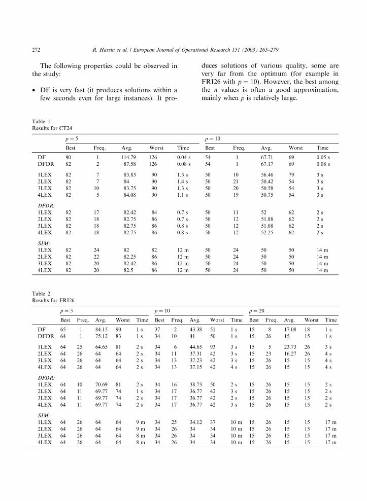
• DF is very fast (it produces solutions within a

few seconds even for large instances). It pro-

Table 1

Results for CT24

p ¼ 5

Best Freq. Avg. Worst Time

DF 90 1 114.79 126 0.04 s

DFDR 82 2 87.58 126 0.08 s

1LEX 82 7 83.83 90 1.3 s

2LEX 82 7 84 90 1.4 s

3LEX 82 10 83.75 90 1.3 s

4LEX 82 5 84.08 90 1.1 s

DFDR:

1LEX 82 17 82.42 84 0.7 s

2LEX 82 18 82.75 86 0.7 s

3LEX 82 18 82.75 86 0.8 s

4LEX 82 18 82.75 86 0.8 s

SIM:

1LEX 82 24 82 82 12 m

2LEX 82 22 82.25 86 12 m

3LEX 82 20 82.42 86 12 m

4LEX 82 20 82.5 86 12 m

Table 2

Results for FRI26

p ¼ 5 p ¼ 10

Best Freq. Avg. Worst Time Best Freq. A

DF 65 1 84.15 90 1 s 37 2 4

DFDR 64 1 75.12 83 1 s 34 10 4

1LEX 64 25 64.65 81 2 s 34 6 4

2LEX 64 26 64 64 2 s 34 11 3

3LEX 64 26 64 64 2 s 34 13 3

4LEX 64 26 64 64 2 s 34 13 3

DFDR:

1LEX 64 10 70.69 81 2 s 34 16 3

2LEX 64 11 69.77 74 1 s 34 17 3

3LEX 64 11 69.77 74 2 s 34 17 3

4LEX 64 11 69.77 74 2 s 34 17 3

SIM:

1LEX 64 26 64 64 9 m 34 25 3

2LEX 64 26 64 64 9 m 34 26 3

3LEX 64 26 64 64 8 m 34 26 3

4LEX 64 26 64 64 8 m 34 26 3

duces solutions of various quality, some are

very far from the optimum (for example in

FRI26 with p ¼ 10). However, the best among

the n values is often a good approximation,mainly when p is relatively large.

p ¼ 10


54 1 67.71 69 0.05 s

54 1 67.17 69 0.08 s

50 10 56.46 79 3 s

50 21 50.42 54 3 s

50 20 50.58 54 3 s

50 19 50.75 54 3 s

50 11 52 62 2 s

50 12 51.88 62 2 s

50 12 51.88 62 2 s

50 12 52.25 62 2 s

50 24 50 50 14 m

50 24 50 50 14 m

50 24 50 50 14 m

50 24 50 50 14 m

p ¼ 20

vg. Worst Time Best Freq. Avg. Worst Time

3.38 51 1 s 15 8 17.08 18 1 s

1 50 1 s 15 26 15 15 1 s

4.65 93 3 s 15 5 23.73 26 3 s

7.31 42 3 s 15 23 16.27 26 4 s

7.23 42 3 s 15 26 15 15 4 s

7.15 42 4 s 15 26 15 15 4 s

8.73 50 2 s 15 26 15 15 2 s

6.77 42 3 s 15 26 15 15 2 s

6.77 42 2 s 15 26 15 15 2 s

6.77 42 3 s 15 26 15 15 2 s

4.12 37 10 m 15 26 15 15 17 m

4 34 10 m 15 26 15 15 17 m

4 34 10 m 15 26 15 15 17 m

4 34 10 m 15 26 15 15 17 m


• The combination, DFDR, in which the output

of DF produces the initial solutions to DR is

a reasonable approximation algorithm. It is still

very fast, but sometimes even its best solution isinferior to those produced by 1LEX.

Table 3

Results for CT30

p ¼ 5


DF 105 1 119.23 143 0.05 s

DFDR 92 12 102.23 118 0.1 s

1LEX 92 16 98.70 118 2 s

2LEX 92 20 96.53 111 2 s

3LEX 92 20 96.53 111 2 s

4LEX 92 20 96.33 105 2 s

DFDR:

1LEX 92 23 95.23 111 1 s

2LEX 92 23 95.03 105 1 s

3LEX 92 23 95.03 105 1 s

4LEX 92 24 94.60 105 1 s

SIM:

1LEX 92 30 92 92 15 m

2LEX 92 30 92 92 15 m

3LEX 92 30 92 92 15 m

4LEX 92 30 92 92 15 m

Table 4

Results for DANTZIG42

p ¼ 5 p ¼ 10


DF 42 1 53.36 60 1 s 28 1 31

DFDR 36 9 41.69 50 1 s 28 5 30

1LEX 38 1 44.67 70 4 s 27 1 32

2LEX 35 4 42.14 46 5 s 26 6 28

3LEX 35 2 41.86 46 5 s 26 9 28

4LEX 35 10 41.45 46 7 s 26 9 28

DFDR:

1LEX 35 16 38.52 43 4 s 27 6 29

2LEX 35 20 38.19 46 4 s 27 5 28

3LEX 35 22 37.81 46 4 s 27 5 28

4LEX 35 30 37.29 46 5 s 27 5 28

SIM:

1LEX 35 42 35 35 14 m 26 19 26

2LEX 35 42 35 35 14 m 26 30 26

3LEX 35 42 35 35 14 m 26 24 26

4LEX 35 40 35.38 43 14 m 26 19 27

• When applying the lexicographic rule in lo-

cal search from random points or from the

results of DFDR, the quality of the solu-

tions usually improved when ‘ grows from 1to 4.

p ¼ 10


61 3 69.63 81 0.07 s

61 4 64.07 70 0.1 s

61 7 64.53 92 5 s

61 8 62.13 66 5 s

61 9 62.03 66 5 s

61 16 61.73 66 6 s

61 8 62.07 66 3 s

61 8 62.07 66 3 s

61 18 61.73 66 5 s

61 20 61.60 66 5 s

61 30 61 61 17 m

61 30 61 61 17 m

61 30 61 61 17 m

61 30 61 61 17 m

p ¼ 20


.79 35 1 s 17 3 18.79 20 2 s

.52 35 2 s 17 18 18.33 20 1 s

.60 45 9 s 15 5 22.38 29 15 s

.60 33 12 s 15 27 16.74 21 21 s

.10 31 13 s 15 33 15.57 21 25 s

31 13 s 15 35 15.36 18 29 s

.17 31 7 s 15 3 16.95 20 15 s

.74 31 9 s 15 4 16.83 18 18 s

.74 31 9 s 15 4 16.83 18 18 s

.83 31 10 s 15 4 16.83 18 20 s

.55 27 16 m 15 42 15 15 20 m

.43 28 16 m 15 42 15 15 20 m

.86 29 16 m 15 42 15 15 20 m

.19 29 16 m 15 42 15 15 20 m


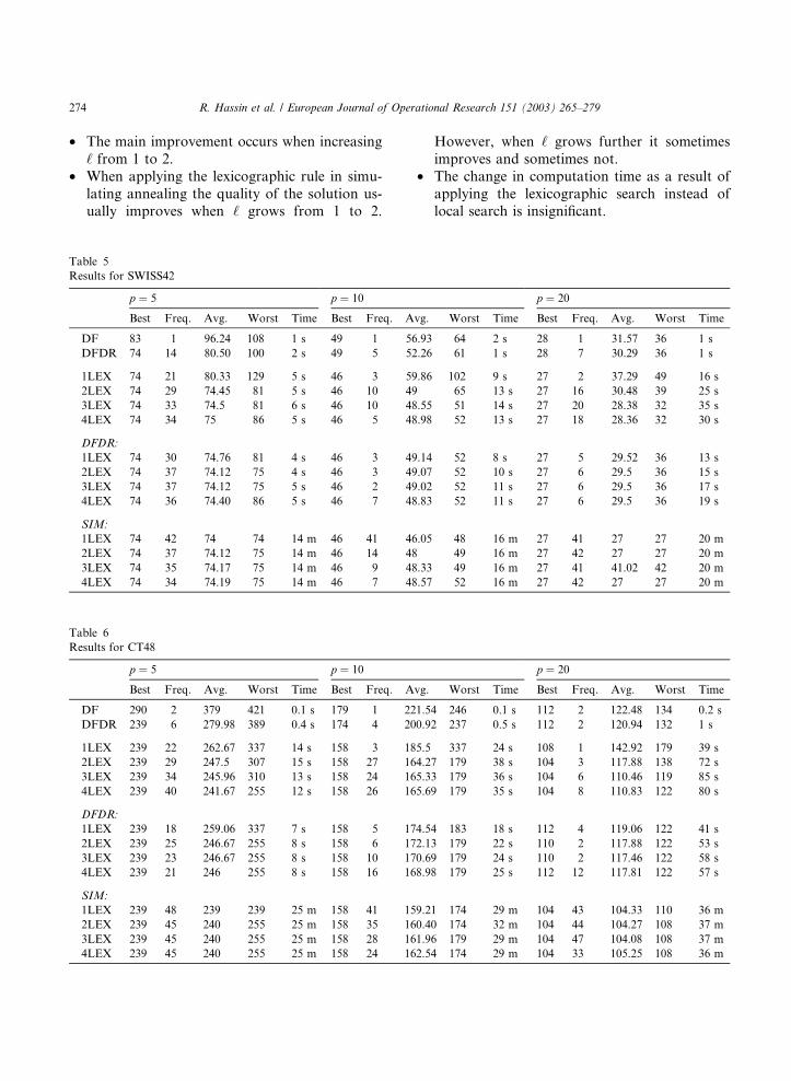
• The main improvement occurs when increasing

‘ from 1 to 2.

• When applying the lexicographic rule in simu-

lating annealing the quality of the solution us-ually improves when ‘ grows from 1 to 2.

Table 5

Results for SWISS42

p ¼ 5 p ¼ 10


DF 83 1 96.24 108 1 s 49 1 56

DFDR 74 14 80.50 100 2 s 49 5 52

1LEX 74 21 80.33 129 5 s 46 3 59

2LEX 74 29 74.45 81 5 s 46 10 49

3LEX 74 33 74.5 81 6 s 46 10 48

4LEX 74 34 75 86 5 s 46 5 48

DFDR:

1LEX 74 30 74.76 81 4 s 46 3 49

2LEX 74 37 74.12 75 4 s 46 3 49

3LEX 74 37 74.12 75 5 s 46 2 49

4LEX 74 36 74.40 86 5 s 46 7 48

SIM:

1LEX 74 42 74 74 14 m 46 41 46

2LEX 74 37 74.12 75 14 m 46 14 48

3LEX 74 35 74.17 75 14 m 46 9 48

4LEX 74 34 74.19 75 14 m 46 7 48

Table 6

Results for CT48

p ¼ 5 p ¼ 10


DF 290 2 379 421 0.1 s 179 1 22

DFDR 239 6 279.98 389 0.4 s 174 4 20

1LEX 239 22 262.67 337 14 s 158 3 18

2LEX 239 29 247.5 307 15 s 158 27 16

3LEX 239 34 245.96 310 13 s 158 24 16

4LEX 239 40 241.67 255 12 s 158 26 16

DFDR:

1LEX 239 18 259.06 337 7 s 158 5 17

2LEX 239 25 246.67 255 8 s 158 6 17

3LEX 239 23 246.67 255 8 s 158 10 17

4LEX 239 21 246 255 8 s 158 16 16

SIM:

1LEX 239 48 239 239 25 m 158 41 15

2LEX 239 45 240 255 25 m 158 35 16

3LEX 239 45 240 255 25 m 158 28 16

4LEX 239 45 240 255 25 m 158 24 16

However, when ‘ grows further it sometimes

improves and sometimes not.

• The change in computation time as a result of

applying the lexicographic search instead oflocal search is insignificant.

p ¼ 20


.93 64 2 s 28 1 31.57 36 1 s

.26 61 1 s 28 7 30.29 36 1 s

.86 102 9 s 27 2 37.29 49 16 s

65 13 s 27 16 30.48 39 25 s

.55 51 14 s 27 20 28.38 32 35 s

.98 52 13 s 27 18 28.36 32 30 s

.14 52 8 s 27 5 29.52 36 13 s

.07 52 10 s 27 6 29.5 36 15 s

.02 52 11 s 27 6 29.5 36 17 s

.83 52 11 s 27 6 29.5 36 19 s

.05 48 16 m 27 41 27 27 20 m

49 16 m 27 42 27 27 20 m

.33 49 16 m 27 41 41.02 42 20 m

.57 52 16 m 27 42 27 27 20 m

p ¼ 20


1.54 246 0.1 s 112 2 122.48 134 0.2 s

0.92 237 0.5 s 112 2 120.94 132 1 s

5.5 337 24 s 108 1 142.92 179 39 s

4.27 179 38 s 104 3 117.88 138 72 s

5.33 179 36 s 104 6 110.46 119 85 s

5.69 179 35 s 104 8 110.83 122 80 s

4.54 183 18 s 112 4 119.06 122 41 s

2.13 179 22 s 110 2 117.88 122 53 s

0.69 179 24 s 110 2 117.46 122 58 s

8.98 179 25 s 112 12 117.81 122 57 s

9.21 174 29 m 104 43 104.33 110 36 m

0.40 174 32 m 104 44 104.27 108 37 m

1.96 179 29 m 104 47 104.08 108 37 m

2.54 174 29 m 104 33 105.25 108 36 m


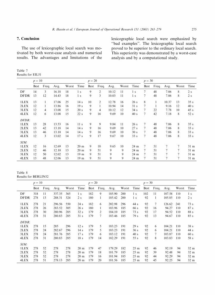
7. Conclusion

The use of lexicographic local search was mo-

tivated by both worst-case analysis and numericalresults. The advantages and limitations of the

Table 7

Results for EIL51

p ¼ 10 p ¼ 20


DF 14 3 16.18 18 1 s 9 2 10

DFDR 13 12 14.43 18 1 s 9 3 10

1LEX 13 1 17.06 25 14 s 10 2 12

2LEX 12 1 13.86 16 19 s 9 1 10

3LEX 12 4 13.08 15 20 s 9 4 10

4LEX 12 6 13.08 15 22 s 9 16 9

DFDR:

1LEX 13 28 13.53 16 11 s 9 9 9

2LEX 13 42 13.18 14 14 s 9 16 9

3LEX 13 46 13.10 14 14 s 9 16 9

4LEX 12 3 13.02 14 17 s 9 17 9

SIM:

1LEX 12 16 12.69 13 20 m 9 18 9

2LEX 12 46 12.10 13 20 m 9 51 9

3LEX 12 50 12.02 13 19 m 9 51 9

4LEX 13 48 12.06 13 19 m 9 51 9

Table 8

Results for BERLIN52

p ¼ 10 p ¼ 20


DF 318 11 337.35 365 1 s 182 9 18

DFDR 278 13 288.31 324 2 s 180 1 18

1LEX 278 21 296.56 550 24 s 182 6 20

2LEX 278 26 283.52 305 26 s 180 1 18

3LEX 278 30 280.96 285 32 s 179 2 18

4LEX 278 31 280.83 285 31 s 179 7 18

DFDR:

1LEX 278 15 285 296 12 s 179 5 18

2LEX 278 24 282.67 296 14 s 179 5 18

3LEX 278 24 281.76 285 17 s 179 6 18

4LEX 278 31 280.83 285 18 s 179 14 18

SIM:

1LEX 278 52 278 278 20 m 179 47 17

2LEX 278 52 278 278 20 m 179 18 18

3LEX 278 52 278 278 20 m 179 16 18

4LEX 278 51 278.13 285 20 m 179 20 18

lexicographic local search were emphasized by

‘‘bad examples’’. The lexicographic local search

proved to be superior to the ordinary local search.

This superiority was demonstrated by a worst-case

analysis and by a computational study.

p ¼ 30


.12 11 1 s 7 48 7.06 8 2 s

.03 11 1 s 7 48 7.06 8 2 s

.78 16 26 s 8 1 10.37 13 35 s

.94 14 31 s 7 1 9.16 12 40 s

.12 12 34 s 7 22 7.78 10 45 s

.69 10 40 s 7 42 7.18 8 52 s

.84 11 26 s 7 48 7.06 8 35 s

.69 10 27 s 7 48 7.06 8 33 s

.69 10 30 s 7 48 7.06 8 33 s

.67 10 33 s 7 48 7.06 8 33 s

.65 10 24 m 7 51 7 7 31 m

9 24 m 7 51 7 7 31 m

9 24 m 7 51 7 7 31 m

9 24 m 7 51 7 7 31 m

p ¼ 30


5.90 200 1 s 102 11 107.58 110 1 s

5.42 200 1 s 92 1 105.85 110 2 s

2.98 296 44 s 92 7 126.62 241 73 s

3.96 185 66 s 92 16 94.27 110 87 s

4.10 185 73 s 92 17 94.52 110 88 s

3.46 185 79 s 92 13 94.67 110 85 s

3.23 191 29 s 92 6 104.21 110 38 s

3.23 191 36 s 92 6 104.21 110 44 s

3.12 191 40 s 92 7 103.87 110 60 s

2.29 191 55 s 92 8 103.83 110 58 s

9.29 182 25 m 92 46 92.19 94 32 m

1.79 185 25 m 92 39 92.48 94 32 m

1.94 185 25 m 92 44 92.29 94 32 m

1.56 185 25 m 92 45 92.25 94 32 m


Appendix A

In this section we show the detailed numerical

results relating to the following instances:

Table 9

Results for BRASIL58

p ¼ 10 p ¼ 20


DF 806 3 937.60 1030 1 s 455 1 5

DFDR 799 1 810.07 932 2 s 446 21 4

1LEX 1000 58 1000 1000 5 s 446 14 7

2LEX 785 3 978.60 1000 15 s 439 3 5

3LEX 785 13 910.95 1000 23 s 439 3 5

4LEX 785 21 860.86 1000 30 s 439 3 4

DFDR:

1LEX 785 7 801.29 806 17 s 446 43 4

2LEX 785 7 801.29 806 17 s 446 38 4

3LEX 785 7 801.29 806 21 s 446 41 4

4LEX 785 7 801.29 806 26 s 446 38 4

SIM:

1LEX 785 58 785 785 23 m 439 44 4

2LEX 785 57 785.24 799 22 m 439 4 4

3LEX 785 24 791.45 806 22 m 446 58 4

4LEX 785 6 802.02 806 23 m 446 57 4

Table 10

Results for ST70

p ¼ 10 p ¼ 20


DF 23 9 25.07 28 1 s 14 9 1

DFDR 21 15 22.84 27 1 s 13 12 1

1LEX 23 1 26.57 43 34 s 15 1 2

2LEX 20 2 23.41 28 44 s 13 10 1

3LEX 19 1 21.56 24 65 s 12 13 1

4LEX 20 31 20.99 24 70 s 12 17 1

DFDR:

1LEX 19 2 21.43 24 34 s 12 2 1

2LEX 19 4 20.63 23 42 s 12 5 1

3LEX 19 6 20.36 23 48 s 12 5 1

4LEX 19 6 20.26 23 50 s 12 5 1

SIM:

1LEX 19 28 19.60 20 44 m 12 19 1

2LEX 19 49 19.30 20 44 m 12 68 1

3LEX 19 56 19.21 21 45 m 12 55 1

4LEX 19 43 19.41 21 44 m 12 58 1

CT24: An instance with 24 nodes from [8].

FRI26: An instance with 26 nodes from [15].


DANTZIG42: An instance with 42 nodes from[15].

p ¼ 30


23.57 544 1 s 262 1 284.74 300 2 s

94.81 544 1 s 260 3 276.88 287 2 s

47.78 1000 59 s 259 2 410.43 1000 104 s

76.22 1000 91 s 259 8 312.52 1000 127 s

04.93 1000 105 s 259 7 287.05 1000 125 s

67.84 1000 115 s 259 11 287.19 1000 129 s

65.69 544 55 s 259 6 265.53 287 79 s

64.74 544 68 s 259 7 265.14 287 82 s

64.28 544 68 s 259 7 264.66 287 102 s

68.98 544 68 s 259 7 264.66 287 90 s

41 455 29 m 259 40 259.31 260 36 m

45.67 455 28 m 259 47 259.29 262 35 m

46 446 28 m 259 53 259.16 262 35 m

46.16 455 28 m 259 56 259.03 260 35 m

p ¼ 30


5.77 18 2 s 9 4 10.14 11 2 s

5.11 18 2 s 9 16 9.94 11 2 s

0.87 33 79 s 11 3 16.26 24 131 s

5.91 19 112 s 9 1 12.04 24 160 s

3.80 19 165 s 9 10 10.60 14 182 s

2.97 19 186 s 9 41 10.07 11 221 s

3.37 16 98 s 9 25 9.76 11 123 s

3.11 14 108 s 9 31 9.64 11 135 s

3.07 14 115 s 9 32 9.63 11 139 s

3.06 14 118 s 9 32 9.63 11 143 s

2.74 14 55 m 9 40 9.49 11 73 m

2.03 13 57 m 9 70 9 9 70 m

2.21 13 57 m 9 70 9 9 70 m

2.17 13 56 m 9 70 9 9 71 m


SWISS42: An instance with 42 nodes from

[15].


EIL51: An instance with 51 nodes from [15].

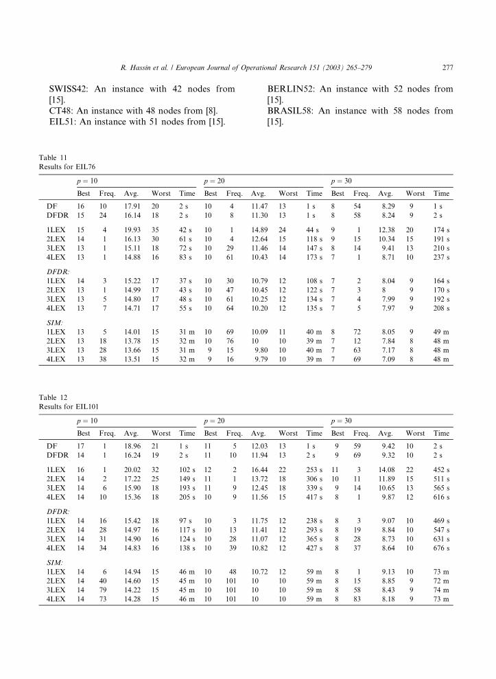
Table 11

Results for EIL76

p ¼ 10 p ¼ 20


DF 16 10 17.91 20 2 s 10 4 1

DFDR 15 24 16.14 18 2 s 10 8 1

1LEX 15 4 19.93 35 42 s 10 1 1

2LEX 14 1 16.13 30 61 s 10 4 1

3LEX 13 1 15.11 18 72 s 10 29 1

4LEX 13 1 14.88 16 83 s 10 61 1

DFDR:

1LEX 14 3 15.22 17 37 s 10 30 1

2LEX 13 1 14.99 17 43 s 10 47 1

3LEX 13 5 14.80 17 48 s 10 61 1

4LEX 13 7 14.71 17 55 s 10 64 1

SIM:

1LEX 13 5 14.01 15 31 m 10 69 1

2LEX 13 18 13.78 15 32 m 10 76 1

3LEX 13 28 13.66 15 31 m 9 15

4LEX 13 38 13.51 15 32 m 9 16

Table 12

Results for EIL101

p ¼ 10 p ¼ 20


DF 17 1 18.96 21 1 s 11 5 1

DFDR 14 1 16.24 19 2 s 11 10 1

1LEX 16 1 20.02 32 102 s 12 2 1

2LEX 14 2 17.22 25 149 s 11 1 1

3LEX 14 6 15.90 18 193 s 11 9 1

4LEX 14 10 15.36 18 205 s 10 9 1

DFDR:

1LEX 14 16 15.42 18 97 s 10 3 1

2LEX 14 28 14.97 16 117 s 10 13 1

3LEX 14 31 14.90 16 124 s 10 28 1

4LEX 14 34 14.83 16 138 s 10 39 1

SIM:

1LEX 14 6 14.94 15 46 m 10 48 1

2LEX 14 40 14.60 15 45 m 10 101 1

3LEX 14 79 14.22 15 45 m 10 101 1

4LEX 14 73 14.28 15 46 m 10 101 1

BERLIN52: An instance with 52 nodes from

[15].

BRASIL58: An instance with 58 nodes from

[15].

p ¼ 30


1.47 13 1 s 8 54 8.29 9 1 s

1.30 13 1 s 8 58 8.24 9 2 s

4.89 24 44 s 9 1 12.38 20 174 s

2.64 15 118 s 9 15 10.34 15 191 s

1.46 14 147 s 8 14 9.41 13 210 s

0.43 14 173 s 7 1 8.71 10 237 s

0.79 12 108 s 7 2 8.04 9 164 s

0.45 12 122 s 7 3 8 9 170 s

0.25 12 134 s 7 4 7.99 9 192 s

0.20 12 135 s 7 5 7.97 9 208 s

0.09 11 40 m 8 72 8.05 9 49 m

0 10 39 m 7 12 7.84 8 48 m

9.80 10 40 m 7 63 7.17 8 48 m

9.79 10 39 m 7 69 7.09 8 48 m

p ¼ 30


2.03 13 1 s 9 59 9.42 10 2 s

1.94 13 2 s 9 69 9.32 10 2 s

6.44 22 253 s 11 3 14.08 22 452 s

3.72 18 306 s 10 11 11.89 15 511 s

2.45 18 339 s 9 14 10.65 13 565 s

1.56 15 417 s 8 1 9.87 12 616 s

1.75 12 238 s 8 3 9.07 10 469 s

1.41 12 293 s 8 19 8.84 10 547 s

1.07 12 365 s 8 28 8.73 10 631 s

0.82 12 427 s 8 37 8.64 10 676 s

0.72 12 59 m 8 1 9.13 10 73 m

0 10 59 m 8 15 8.85 9 72 m

0 10 59 m 8 58 8.43 9 74 m

0 10 59 m 8 83 8.18 9 73 m

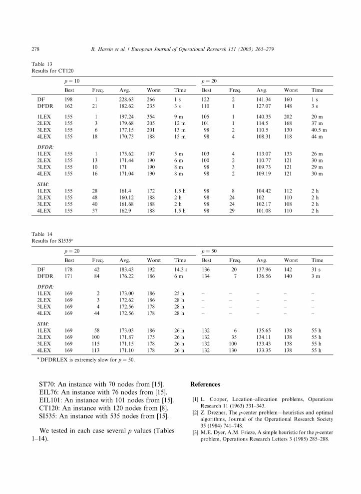
Table 13

Results for CT120

p ¼ 10 p ¼ 20

Best Freq. Avg. Worst Time Best Freq. Avg. Worst Time

DF 198 1 228.63 266 1 s 122 2 141.34 160 1 s

DFDR 162 21 182.62 235 3 s 110 1 127.07 148 3 s

1LEX 155 1 197.24 354 9 m 105 1 140.35 202 20 m

2LEX 155 3 179.68 205 12 m 101 1 114.5 168 37 m

3LEX 155 6 177.15 201 13 m 98 2 110.5 130 40.5 m

4LEX 155 18 170.73 188 15 m 98 4 108.31 118 44 m

DFDR:

1LEX 155 1 175.62 197 5 m 103 4 113.07 133 26 m

2LEX 155 13 171.44 190 6 m 100 2 110.77 121 30 m

3LEX 155 10 171 190 8 m 98 3 109.73 121 29 m

4LEX 155 16 171.04 190 8 m 98 2 109.19 121 30 m

SIM:

1LEX 155 28 161.4 172 1.5 h 98 8 104.42 112 2 h

2LEX 155 48 160.12 188 2 h 98 24 102 110 2 h

3LEX 155 40 161.68 188 2 h 98 24 102.17 108 2 h

4LEX 155 37 162.9 188 1.5 h 98 29 101.08 110 2 h

Table 14

Results for SI535a

p ¼ 20 p ¼ 50

Best Freq. Avg. Worst Time Best Freq. Avg. Worst Time

DF 178 42 183.43 192 14.3 s 136 20 137.96 142 31 s

DFDR 171 84 176.22 186 6 m 134 7 136.56 140 3 m

DFDR:

1LEX 169 2 173.00 186 25 h – – – – –

2LEX 169 3 172.62 186 28 h – – – – –

3LEX 169 4 172.56 178 28 h – – – – –

4LEX 169 44 172.56 178 28 h – – – – –

SIM:

1LEX 169 58 173.03 186 26 h 132 6 135.65 138 55 h

2LEX 169 100 171.87 175 26 h 132 35 134.11 138 55 h

3LEX 169 115 171.15 178 26 h 132 100 133.43 138 55 h

4LEX 169 113 171.10 178 26 h 132 130 133.35 138 55 h

aDFDRLEX is extremely slow for p ¼ 50.


ST70: An instance with 70 nodes from [15].




SI535: An instance with 535 nodes from [15].

We tested in each case several p values (Tables1–14).

References

[1] L. Cooper, Location–allocation problems, Operations

Research 11 (1963) 331–343.

[2] Z. Drezner, The p-center problem––heuristics and optimal

algorithms, Journal of the Operational Research Society

35 (1984) 741–748.

[3] M.E. Dyer, A.M. Frieze, A simple heuristic for the p-centerproblem, Operations Research Letters 3 (1985) 285–288.


[4] R.J. Fowler, M.S. Paterson, S.L. Tanimoto, Optimal

packing and covering in the plane are NP-complete,

Information Processing Letters 12 (1987) 133–137.

[5] M. F€uurer, B. Raghavachari, Approximating the minimum

degree spanning tree to within one from the optimal

degree, in: Proceedings of the Third Annual ACM-SIAM

Symposium on Discrete Algorithms, 1992.

[6] M. F€uurer, B. Raghavachari, Approximating the minimum

degree Steiner tree to within one of optimal, Journal of

Algorithms 17 (1994) 409–423.

[7] C.A. Glass, C.N. Potts, P. Shade, Unrelated parallel

machine scheduling using local search, Mathematical and

Computer Modeling 20 (1994) 41–52.

[8] M. Gr€ootschel, O. Holland, Solution of large-scale sym-

metric travelling salesman problems, Mathematical Pro-

gramming 51 (1991) 141–202.

[9] G.Y. Handler, P. Mirchandani, Location on Networks,

Theory and Algorithms, M.I.T. Press, Cambridge, MA,

1979.

[10] D.S. Hochbaum, D.B. Shmoys, A best possible heuristic

for the k-center problem, Mathematics of Operations

Research 10 (1985) 180–184.

[11] D.S. Hochbaum, D.B. Shmoys, A unified approach to

approximation algorithms for bottleneck problems, Jour-

nal of the Association for Computing Machinery 33 (1986)

533–550.

[12] S. Khanna, R. Motwani, M. Sudan, U. Vazirani, On

syntactic versus computational views of approxima-

bility, in: Proceedings of the 35th Annual IEEE Sym-

posium on Foundations of Computer Science, 1994,

pp. 819–830.

[13] J. Plesn�ıık, A heuristic for the p-center problem in graphs,

Discrete Applied Mathematics 17 (1987) 263–268.

[14] J. Plesn�ıık, On the interchange heuristic for locating centers

and medians in a graph, Mathematica Slovaca 37 (1987)

209–216.

[15] G. Reinelt, TSPLIB. Available from <ftp://elib.zib-ber-

lin.de/pub/mp-testdata/tsp/index.html>.

ftp://elib.zib-berlin.de/pub/mp-testdata/tsp/index.html

ftp://elib.zib-berlin.de/pub/mp-testdata/tsp/index.html

lexicographic local search and the p-center problem

Documents