leverage aversion and risk parity - cloud object …s3.amazonaws.com/zanran_storage/ aversion and...

1

Leverage Aversion and Risk Parity

Cliff Asness, Andrea Frazzini, and Lasse H. Pedersen*

This draft: December 27, 2010

Abstract.

Leverage aversion changes the predictions of modern portfolio theory: It causes safe assets to

offer higher risk-adjusted returns than riskier assets. Consuming the high risk-adjusted

returns offered by safe assets requires leverage, creating an opportunity for investors with the

ability and willingness to borrow. A Risk Parity (RP) portfolio exploits this in a simple way,

namely by equalizing the risk allocation across asset classes, thus overweighting safe assets

relative to their weight in the market portfolio. We show empirically that RP has

outperformed the market over the last century by a statistically and economically significant

amount.

* Cliff Assess is at AQR Capital Management, Two Greenwich Plaza, Greenwich, CT 06830, email: [email protected]. Andrea Frazzini is at AQR Capital Management, Two Greenwich Plaza, Greenwich, CT 06830, e-mail: [email protected]. Lasse H. Pedersen is at New York University, AQR, NBER, and CEPR, 44 West Fourth Street, NY 10012-1126; e-mail: [email protected]; web: http://www.stern.nyu.edu/~lpederse/. We would like to thank John Liew for helpful comments and discussions.

Leverage Aversion and Risk Parity – Cliff Asness, Andrea Frazzini and Lasse H. Pedersen –

How should investors allocate their assets? The standard advice provided by the Sharpe-

Lintner-Mossin Capital Asset Pricing Model (CAPM) is that all investors should hold the

market portfolio, leveraged according to each investor’s risk preference. However, over

recent years a new approach to asset allocation called Risk Parity (RP) has surfaced and has

been gaining in popularity among practitioners. We fill what we believe is a hole in the

current arguments in favor of Risk Parity investing by adding a theoretical justification based

on investors’ aversion to leverage and by providing broad empirical evidence.

Risk Parity investing starts from the observation that traditional asset allocations, such

the market portfolio or the 60/40 portfolio in U.S. stocks/bonds, are insufficiently diversified

when viewed from the perspective of how each investment contributes to the risk of the

overall portfolio. Because stocks are so much more volatile than bonds, movement in the

stock market dominates the risk in a 60/40 portfolio. Thus, when viewed from a risk

perspective, 60/40 is mainly an equity portfolio. In this sense, 60/40 offers little

diversification even though 60/40 looks well balanced when viewed from the perspective of

dollars invested in each asset class.

Risk Parity advocates suggest a simple cure: Be diversified, but be diversified by risk

not by dollars. That is, take a similar amount of risk in equities and in bonds. To diversify by

risk, we generally need to invest more money in low-risk assets than in high risk assets. As a

result, even if return-per-unit-of-risk is higher, the total aggressiveness and expected return is

lower than that of a traditional 60/40 portfolio. Risk Parity investors address this problem by

applying leverage to the risk-balanced portfolio to increase its risk and expected return to

desired levels. While you do introduce the practical concern of using leverage (a topic for

another day), now you have the best of both worlds: You are truly risk (not dollar) balanced

across the asset classes and, importantly, you are taking enough risk to matter. Details can

vary tremendously (for instance, real life Risk Parity is about much more than just U.S.

stocks and bonds), but the above is the essence of Risk Parity investing.

To further bolster the case for Risk Parity investing, beyond simply the idea that more

diversification must be better, advocates appeal to the historical experience that Risk Parity

portfolios have done better than traditional portfolios. Figure 1 shows the growth of $1 since

1926 in a 60/40 portfolio, in a portfolio that weights by the ex-ante market cap of each asset

class, and, finally, in a simple version of a Risk Parity portfolio. While we show one case


here, the historical outperformance of Risk Parity is quite robust. In sum, the popular case

for Risk Parity investing rests on (1) the intuitive superiority of balancing risk and not dollars

invested and (2) the historical evidence for this approach over traditional approaches.

While these arguments are alluring, unfortunately, we don’t think they are enough.

Starting with (1) above, the intuition that a risk balanced portfolio is always better, is simply

false. You don’t always want to be as risk balanced as possible. For instance, if the expected

return of stocks was high enough versus bonds (a high enough “equity risk premium”) you

would gladly invest in a portfolio whose risk was equity dominated. The intuition of “equal

risk” is only accurate in the specific case of each asset possessing equal risk adjusted returns.

The intuition that 60/40 investors take too much risk in equities at all is only accurate if the

equity risk premium versus bonds is not high enough.

In other words, you can’t just assert that equal risk is optimal. Rather, to believe that,

you must believe you are not getting paid enough in equities to be so concentrated in them.

You cannot think of Risk Parity as only a statement about divvying up risks, as it’s inherently

also a statement about your views on expected return. A Risk Parity investor should not say

“equal risk is always the best regardless of expected returns.” Instead, they should say “we

do not believe expected returns are high enough on equities to make them a disproportionate

part of our risk budget.” That’s an important distinction lost in the current discussion of Risk

Parity. In fact, according to the CAPM, the risk premia are exactly such that the market

portfolio is optimal, so Risk Parity investors need to explain how the CAPM fails in a way

that justifies a larger allocation to low-risk assets.

Let’s turn to (2), the empirical support that a Risk Parity portfolio has outperformed

over the long-term. It is indeed useful and relevant evidence in favor of Risk Parity, but it’s

also only one draw from history (admittedly a decently long one). We have to ask if this is

enough? Does the equity premium over bonds not being large enough in the last 80+ years

mean it won’t be large enough going forward? Ideally, we would like to have some out-of-

sample evidence, but waiting another 80 years seems an unappealing strategy. We propose

another route to potentially increasing our confidence.

The missing links are i) a theoretical justification for Risk Parity investing, combined

with ii) broad tests across and within the major asset classes. Frazzini and Pedersen (2010)


present these links. Following Fischer Black (1972), they show that if some investors are

adverse to leverage, low-beta assets will offer higher risk-adjusted returns, and high-beta

assets lower risk-adjusted returns. Leverage aversion breaks the standard CAPM, and

according to this theory the highest risk-adjusted return is not achieved by the market, but by

a portfolio that over-weights safer assets. Thus, an investor who is less leverage averse (or

less leverage constrained) than the average investor can benefit by overweighting low-beta

assets, underweighting high-beta assets, and applying some leverage to the resulting

portfolio.

Empirically, Frazzini and Pedersen (2010) find consistent evidence of this theory within

each major asset class. They find that low-beta stocks have higher risk-adjusted returns than

high-beta stocks in the U.S. (echoing Black, Jensen, and Scholes (1972)) and in global stock

markets, safer corporate bonds have higher risk-adjusted returns than riskier ones, safer

short-maturity Treasuries offer higher risk-adjusted returns than riskier long-maturity ones,

and similarly within several other asset classes.1

As applied to Risk Parity, bonds are the low-beta asset, stocks the high-beta asset, and

the benefit of over-weighting bonds is another empirical success of the theory. The theory of

leverage aversion not only constitutes a theoretical underpinning for Risk Parity, but it also

highlights how further out-of-sample empirical evidence can be achieved by comparing the

risk-adjusted returns of safe vs. riskier securities within each of the major asset classes.

Having the theory hold up in many other applications (without notable exception) completely

separate from the asset allocation decision studied here, makes us far more confident that the

empirical superiority of Risk Parity is not a statistical fluke, but rather one more feather in

the cap of Fisher Black’s theory, and one more instance to add to the many in Frazzini and

Pedersen (2010).2

1 This evidence complements that large literature documenting that the CAPM is violated empirically (Fama and French (1992), Gibbons (1982), Kandel (1984), Karceski (2002), Shanken (1985)). Given the strong assumptions underlying the CAPM, it should perhaps not be a surprise that it is rejected empirically. Indeed, the CAPM assumes that markets are without any frictions and that all investors can use any amount of leverage. According to the CAPM, everyone holds the market portfolio (possibly leveraged) – which is clearly not the case in the real world. However, that these violations tend to go the same way, higher returns on low beta assets than forecast, is very interesting. 2 Naturally, there are other hypotheses that produce higher risk-adjusted returns of safe assets versus riskier assets. The alternatives include models of delegated portfolio managements with benchmarked institutional investor (Brennan (1993), Baker, Bradley, and Wurgler (2010)), mutual fund managers’ incentive to over-


The rest of the paper is organized as follows. First we lay out our theory of leverage

aversion. We present the investment opportunity set for investors who cannot use leverage.

As an alternative to leverage, these investors overweight riskier asset, and this increases the

equilibrium price of riskier assets or, said differently, reduces the expected return on riskier

assets. As a result, if some investors face such leverage constraints or margin requirements,

then the market portfolio is not the portfolio with the highest Sharpe ratio as the standard

CAPM predicts. Instead, the portfolio with the highest Sharpe ratio over-weights safer assets

and under-weights riskier assets, just like the RP portfolio. Next we test the theory's

implications for asset allocation. We find that the portfolio with the highest ex post Sharpe

indeed over-weights safe asset classes. Further, we find that the implementable RP portfolio

is close to the (unimplementable) ex post optimal portfolio. Finally we test the theory's

predictions for security selection within asset classes, finding strong consistent evidence that

safer assets offer higher risk-adjusted returns than riskier ones. This is important as it is out-

of-sample evidence that our story for risk-parity is not limited to the successful history

documented in Figure 1. Details about our data and portfolio construction are in Appendix.

A Theory of Leverage Aversion

Before we introduce leverage aversion, let us revisit the standard predictions of Modern

Portfolio Theory (MPT) of Markowitz (1952) and the Capital Asset Pricing Model (CAPM)

of Sharpe (1964), Lintner (1965) and Mossin (1966). MPT considers how an investor should

choose a portfolio with a good trade-off between risk and expected return. This is often

illustrated using a mean-volatility diagram as in Figure 2, which uses data from 1926 to

2010. The figure shows that the overall stock market has had average returns of 7.4% per

year with a volatility of 16.0%, while the overall bond market provided a lower average

return of 5.2% at a lower volatility of 3.4%. The hyperbola connecting these two points

represents all possible portfolios of stocks and bonds. For instance, the 60-40 portfolio

represents an investment of 60% of capital in stocks and 40% of capital in bonds. (This

weight high beta stocks due to the option-like payoffs generated by the convexity of the flow-performance relation (Falkenstein (1994) and Karceski (2002)), or money illusion (Cohen, Polk, and Vuolteenaho (2005)). These alternatives are not mutually exclusive but they deliver predictions that apply to a specific setting (for example the universe of active equity mutual fund managers), as a result each of these alternatives can explain some but all the evidence within and across each of the major asset classes. They can of course be complementary to our unified leverage aversion theory.


portfolio is rebalanced every month to these weights.)

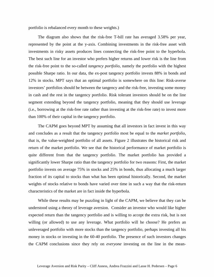
The diagram also shows that the risk-free T-bill rate has averaged 3.58% per year,

represented by the point at the y-axis. Combining investments in the risk-free asset with

investments in risky assets produces lines connecting the risk-free point to the hyperbola.

The best such line for an investor who prefers higher returns and lower risk is the line from

the risk-free point to the so-called tangency portfolio, namely the portfolio with the highest

possible Sharpe ratio. In our data, the ex-post tangency portfolio invests 88% in bonds and

12% in stocks. MPT says that an optimal portfolio is somewhere on this line: Risk-averse

investors’ portfolios should be between the tangency and the risk-free, investing some money

in cash and the rest in the tangency portfolio. Risk tolerant investors should be on the line

segment extending beyond the tangency portfolio, meaning that they should use leverage

(i.e., borrowing at the risk-free rate rather than investing at the risk-free rate) to invest more

than 100% of their capital in the tangency portfolio.

The CAPM goes beyond MPT by assuming that all investors in fact invest in this way

and concludes as a result that the tangency portfolio most be equal to the market portfolio,

that is, the value-weighted portfolio of all assets. Figure 2 illustrates the historical risk and

return of the market portfolio. We see that the historical performance of market portfolio is

quite different from that the tangency portfolio. The market portfolio has provided a

significantly lower Sharpe ratio than the tangency portfolio for two reasons: First, the market

portfolio invests on average 75% in stocks and 25% in bonds, thus allocating a much larger

fraction of its capital to stocks than what has been optimal historically. Second, the market

weights of stocks relative to bonds have varied over time in such a way that the risk-return

characteristics of the market are in fact inside the hyperbola.

While these results may be puzzling in light of the CAPM, we believe that they can be

understood using a theory of leverage aversion. Consider an investor who would like higher

expected return than the tangency portfolio and is willing to accept the extra risk, but is not

willing (or allowed) to use any leverage. What portfolio will he choose? He prefers an

unleveraged portfolio with more stocks than the tangency portfolio, perhaps investing all his

money in stocks or investing in the 60-40 portfolio. The presence of such investors changes

the CAPM conclusions since they rely on everyone investing on the line in the mean-


volatility diagram. Specifically, the tangency portfolio is not equal to the market portfolio

when there exist leverage averse investors.

So what is the tangency portfolio? Frazzini and Pedersen (2010) show that the tangency

portfolio over-weights safer assets, just as is the case empirically. This result is intuitive:

Since some investors choose to overweight riskier assets to avoid leverage, the price of

riskier assets is elevated or, equivalently, the expected return on riskier assets is reduced. In

contrast, the safe assets are under-weighted by these investors, and therefore trade at low

prices, i.e., offer high returns. Hence, investors who are able to apply leverage can achieve

higher risk-adjusted returns by having the opposite portfolio tilts, namely over-weighting

safe assets. This is why the tangency portfolio consists of a disproportional amount of safe

assets.

The specific composition of the tangency portfolio depends on how many leverage

constrained investors there are and this can change over time. Hence, in practice, we cannot

know for sure what the tangency portfolio is. However, Risk Parity (RP) investment offers a

simple suggestion, which is in the direction suggested by the leverage aversion theory: RP

investments allocate the same amount of risk to stocks and bonds. This means investing 15%

in stocks and 85% in bonds on an unlevered basis, on average. Figure 2 shows that the

historical performance of the RP portfolio is more similar to that of the tangency portfolio

than either the market or the 60-40 portfolios. As seen in the Figure 2, despite being not

exactly ex post optimal, the RP portfolio has been as good approximation since over-

weighting safe assets has paid off. While we should not take the precise prescription to have

exactly equal risk in stocks and bonds (parity) too seriously, it is quite a strong and accurate

move in the right direction ex post.

The leverage aversion theory is laid out more formally by Frazzini and Pedersen

(2010), who also present several other testable asset pricing predictions. Further, according to

this theory, no one holds the market portfolio, but equilibrium is achieved nevertheless since

some investors over-weight safe assets while others over-weight riskier assets. Both groups

of investors are satisfied: Some accept low Sharpe ratios but achieve high expected returns

without leverage; others achieve high expected returns with a better risk-return tradeoff by

using leverage.


Risk and Return Across Asset Classes: The Market vs. Risk Parity vs. 60-40

To test our predicted implications of leverage aversion, we compare the historical

performance of the value-weighted market portfolio, the Risk Parity portfolio, and the 60-40

stock/bond portfolio. We do this over two different data samples: Our “Long Sample” covers

U.S. stocks and bonds from 1926 to 2010, and our “Broad Sample” covers global stocks,

U.S. bonds, credit, and commodities from 1973 to 2010. Summary statistics are seen in Table

1 and further details on the data and the portfolios are in the appendix.

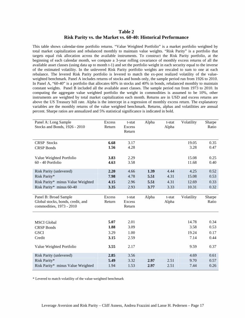
Table 2 shows the performance statistics, with Panel A using our Long Sample, while

Panel B covers the Broad Sample. In both cases, we see that stocks have delivered higher

average returns than bonds, and stocks have realized much higher volatility than bonds. As a

result, the value-weighted market portfolio and the 60-40 portfolio have had higher average

returns than the unleveraged Risk Parity portfolio. Therefore, an investor who cannot and or

will not use leverage may prefer to hold the market or the 60-40 portfolio or even all stocks,

and such behavior is what can cause riskier assets to be overpriced relative to the standard

CAPM.

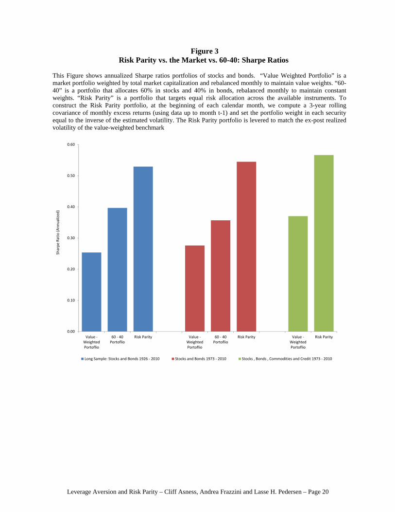
An investor who is able to use leverage will prefer the historical performance of the

Risk Parity portfolio, however, because of its higher Sharpe ratio (risk-adjusted return).

Indeed, the leveraged Risk Parity portfolio has the same volatility as the market portfolio, but

a considerably higher average return. Figure 3 illustrates the significant improvement in

Sharpe ratio of the Risk Parity portfolio over the market and 60-40 portfolios.

The strong historical performance of Risk Parity is also seen in the cumulative return

plot illustrated in Figure 1 (as discussed in the introduction). To test the significance of this

outperformance, Table 2 reports t-statistic of the Risk Parity portfolio’s realized alpha. Here,

alpha is the intercept in a time series regression of monthly excess return on the value-

weighted benchmark. The t-statistics are far north of 2 implying strong statistical

significance. As a further test, we construct long-short portfolios that go long the Risk Parity

portfolio and go short the market portfolio (or go short the 60-40 portfolio) over each sample.

These long-short portfolios have statistically significant excess returns and alphas over both

our Long Sample and our Broad Sample.

A classic illustration of the empirical failure of the standard CAPM is the notion that


the “Security Market Line is too flat,” originally pointed out by Black, Jensen, and Scholes

(1972) for U.S. stocks. The Security Market Line is the connection between the actual excess

return across securities and the CAPM-predicted excess returns, given by beta times the

market excess return. Rather than looking at the Security Market Line across stocks, we are

interested in the Security Market Line across assets classes. Figure 4 shows the Security

Market Line for the asset classes in our Broad Sample, where betas are the slopes from a

time series regression of monthly excess return on the value-weighted benchmark.

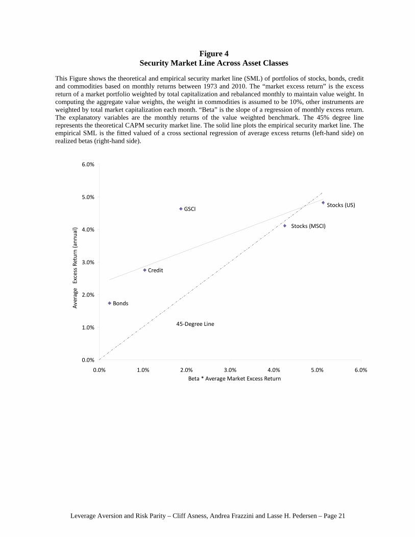
The CAPM predicts that securities line up on the 45 degree line. However, Figure 4

shows that the empirical Security Market Line is more flat since safe asset classes (bonds and

credit) provide too high returns relative to the CAPM, while riskier asset classes (domestic

and global stocks) provide too low returns relative to their risk. The same result (a flat asset

class Security Market Line) is also true for our Long Sample as shown by Figure 1.

Risk and Return Within Asset Classes: High Beta is Low Alpha

Our evidence that the Security Market Line is too flat holds not just across asset

classes, but also within asset classes. Said differently, safe assets have higher risk-adjusted

returns than riskier assets when comparing securities within the same asset class, just as in

the case of comparing across asset classes.

Indeed, Black, Jensen and Scholes (1972) famously found that the Security Market

Line is too flat across U.S. stocks. Frazzini and Pedersen (2010) confirm this finding adding

40 years of out-of-sample evidence: the Security Market Line has remained remarkably flat

since the study of Black, Jensen and Scholes. Further, Frazzini and Pedersen (2010) find that

the Security Market Line is also too flat in all the other major asset classes. It is too flat in

global stocks markets, in 18 of 19 developed equity markets, too flat across Treasuries,

across corporate bonds, and even across futures.

Figure 5 reports the evidence of Frazzini and Pedersen (2010) across U.S. stocks (Panel

A) and across bonds (Panel B). In each case, we see that the Security Market Line is flatter

than the CAPM-predicted 45-degree line, meaning that safe assets provide higher risk-

adjusted returns.

The within-asset-class results are very important to the inherently across-asset-class


results of risk-parity, as they represent strong out-of-sample confirmation that what’s going

on for asset classes is ubiquitous and thus less likely data mining.

Conclusion: You Can Eat Risk Adjusted Returns

Risk Parity investing has become a popular alternative to traditional methods of

strategic asset allocation. However, existing justifications leave a lot to be desired. It is not

enough to simply desire diversification by risk not dollars, however intuitive. If you were

paid enough in expected return to be dominated in risk-space by a single asset class you'd do

so gladly. It's not enough to show that historically you have not in fact been paid enough to

be so dominated (the equivalent of a backtest showing that Risk Parity is historically superior

to traditional allocations). Historical evidence is always welcome, but even long histories of

asset class return can be dominated by a few large data points or arise from data mining.

Risk Parity investors need not despair, however. While there is no certainty in finance,

perhaps the closest we ever come is a realistic theory that holds up consistently in out of

sample tests across and within different asset classes. Leverage aversion, pioneered by Black

(1972) is such a theory.

Assuming that some market participants are unable or unwilling to use leverage is not

unrealistic. Indeed, using leverage requires acquiring a certain “technology” to apply the

leverage, and to manage the leverage and the dynamic portfolio over time. Our capital

markets present plenty of examples of investors that are not allowed (or choose not) to

employ leverage to increase their returns. For example, the majority of mutual funds and

many pension funds are prevented from borrowing or limited in the amount leverage they

can take. As another example, mutual fund families typically provide suggested asset

allocations for low to high risk tolerant investors. The high risk recommendations rarely use

leverage, but rather recommend a very extreme concentration in equities. Similarly, the rise

of embedded leverage in exchange traded funds (ETFs) shows that some investors choose not

to employ leverage directly, but prefer instruments with embedded leverage.

The results in Black, Jensen, and Scholes (1972) and Frazzini and Pedersen (2010)

show that the predictions of a theory of leverage aversion hold up in a very wide variety of

tests across and within many asset classes. This paper shows that Risk Parity investing is


simply another instance of this theory working out of sample, and thus greatly enhances our

confidence that Risk Parity's superiority to traditional methods is not a figment of the data

but real and important.


References

Ashcraft, A., N. Garleanu, and L.H. Pedersen (2010), “Two Monetary Tools: Interest Rates

and Haircuts,” NBER Macroeconomics Annual, forthcoming.

Asness, C.S. (1996), “Why Not 100% Equities,” The Journal of Portfolio Management, Vol.

22:2, 29-34.

Baker, M., B. Bradley, and J. Wurgler (2010), “Benchmarks as Limits to Arbitrage:

Understanding the Low Volatility Anomaly,” working paper, Harvard.

Black, F. (1972), “Capital market equilibrium with restricted borrowing,” Journal of

business, 45, 3, pp. 444-455.

– (1992), “Beta and Return,” The Journal of Portfolio Management, 20, pp. 8-18.

Black, F., M.C. Jensen, and M. Scholes (1972), “The Capital Asset Pricing Model: Some

Empirical Tests.” In Michael C. Jensen (ed.), Studies in the Theory of Capital Markets, New

York, pp. 79-121.

Brennan, M.J. (1993), “Agency and Asset Pricing.” University of California, Los Angeles,

working paper.

Brunnermeier, M. and L.H. Pedersen (2009), “Market Liquidity and Funding Liquidity,” The

Review of Financial Studies, 22, 2201-2238.

Cohen, R.B., C. Polk, and T. Vuolteenaho (2005), “Money Illusion in the Stock Market: The

Modigliani-Cohn Hypothesis,” The Quarterly Journal of Economics, 120:2, 639-668.

Falkenstein, E.G. (1994), “Mutual funds, idiosyncratic variance, and asset returns”,

Dissertation, Northwestern University.


Fama, E.F. and French, K.R. (1992), “The cross-section of expected stock returns,” Journal

of Finance, 47, 2, pp. 427-465.

Frazzini, A. and L. H. Pedersen (2010), “Betting Against Beta”, working paper, AQR Capital

Management, New York University and NBER (WP 16601).

Garleanu, N., and L. H. Pedersen (2009), “Margin-Based Asset Pricing and Deviations from

the Law of One Price," UC Berkeley and NYU, working paper.

Gibbons, M. (1982), “Multivariate tests of financial models: A new approach,” Journal of

Financial Economics, 10, 3-27.

Kandel, S. (1984), “The likelihood ratio test statistic of mean-variance efficiency without a

riskless asset,” Journal of Financial Economics, 13, pp. 575-592.

Karceski, J. (2002), “Returns-Chasing Behavior, Mutual Funds, and Beta’s Death,” Journal

of Financial and Quantitative Analysis, 37:4, 559-594.

Lintner, J. (1965), “The valuation of risk assets and the selection of risky investments in

stock portfolios and capital budgets”, Review of Economics and Statistics, 47, 13-37.

Markowitz, H.M. (1952), “Portfolio Selection,” The Journal of Finance, 7, 77-91.

Mossin, J. (1966), “Equilibrium in a Capital Asset Market”, Econometrica, 34, 768–783.

Shanken, J. (1985), “Multivariate tests of the zero-beta CAPM,” Journal of Financial

Economics, 14,. 327-348.

Sharpe, W. F. (1964), “Capital asset prices: A theory of market equilibrium under conditions

of risk”, Journal of Finance, 19, 425-442.


Appendix: Data and Portfolio Construction

Our study focuses on a Long Sample from January 1926 to June 2010 which consists of

U.S. stocks and government bonds, and a Broad Sample from January 1973 to June 2010

which consists of global stocks, bonds, corporate bonds, and commodities.

The data for the Long Sample is drawn from the CRSP database. We use the CRSP

value weighted market return (including dividends) as the aggregate stock return. Similarly,

our aggregate bond return is the value-weighted average of the unadjusted holding period

return for each bond in the CRSP Monthly US Treasury Database. Bonds are weighted by

their outstanding face value.

To include data on global stocks, commodities, and credit in our Broad Sample, we

need to the more recent time period from 1973. Our global stock market proxy is the MSCI

Word index provided by MSCI/Barra.3 For corporate bonds, we use the Barclays aggregate

US Credit index from Barclays Capital’s Bond.Hub database.4 Finally, we use the S&P GSCI

index as a benchmark for investment in commodity markets obtained from Bloomberg.5

Unfortunately, the commodities series is the only asset class for which we lack a source of

monthly total market capitalization, thus forcing us to make an assumption when

constructing value-weighted aggregate benchmarks. We assume a constant market weight of

10% on commodities. All returns and market capitalization series are in USD and excess

returns are above the US Treasury bill rate.

Constructing Risk Parity Portfolios

We construct simple Risk Parity portfolios (hereafter RP) that are rebalanced monthly

such as to target an equal risk allocation across the available asset classes. To construct a RP

portfolio, at the beginning of each calendar month, we estimate volatilities i of all the

available asset classes (using data up to month t-1) and set the portfolio weight in security i

to:

3 The data can be downloaded at: http://www.mscibarra.com 4 The data can be downloaded at https://live.barcap.com 5 Formerly the Goldman Sachs Commodity Index


nikw ittit ,..,1ˆ 1,,

We estimate i as the 3-year rolling volatility of monthly excess returns, but we get similar

results for other volatility estimates. The constant tk is a constant (same for all assets), which

controls the amount of leverage (or the target volatility) of the RP portfolio.

We consider two very simple RP portfolios: The first portfolio is an unlevered RP,

obtained by setting

i

itk 1

This corresponds to a simple value-weighted portfolio that over-weighted less volatile assets

and under-weight more volatile assets.

The second portfolio is a levered RP obtained by setting

kkt

for all periods. Of course, since k is constant across periods, the exact level of k does not

affect statistical inference. For comparison purposes, we set k so that the average annualized

volatility of this portfolio matches the ex-post realized volatility of the value-weighted

benchmark. This portfolio corresponds to a portfolio targeting a constant volatility in each

asset class, levered up to match the volatility of the value weighted benchmark. (We get

similar results if we choose k to match the volatility of the benchmark at the time of portfolio

formation.)

Portfolios are rebalanced every calendar month and the monthly excess return over T-

bills is given by

)( ,,1 titi

itRP

t rfrwr

where r is the month-t USD gross return and rf is the 1-month Treasury bill rate. Table A1

reports the list of instruments.


Table 1 Summary Statistics

This table reports the list of instruments included in our data and the corresponding date range.

Asset Class Index ME available

Start Year End Year

Long Sample

Stocks CRSP Value-Weighted Index Y 1926 2010

Bonds CRSP Value-Weighted Index Y 1926 2010

Broad Sample

Global stocks MSCI Global Index Y 1973 2010

Bonds CRSP Value-Weighted Index Y 1973 2010

Credit Barclays Capital Credit Index Y 1973 2010

Commodities GSCI N 1973 2010


Table 2 Risk Parity vs. the Market vs. 60-40: Historical Performance

This table shows calendar-time portfolio returns. “Value Weighted Portfolio” is a market portfolio weighted by total market capitalization and rebalanced monthly to maintain value weights. “Risk Parity” is a portfolio that targets equal risk allocation across the available instruments. To construct the Risk Parity portfolio, at the beginning of each calendar month, we compute a 3-year rolling covariance of monthly excess returns of all the available asset classes (using data up to month t-1) and set the portfolio weight in each security equal to the inverse of the estimated volatility. In the unlevered Risk Parity portfolio weights are rescaled to sum to one at each rebalance. The levered Risk Parity portfolio is levered to match the ex-post realized volatility of the value-weighted benchmark. Panel A includes returns of stocks and bonds only, the sample period run from 1926 to 2010. In Panel A, “60-40” is a portfolio that allocates 60% in stocks and 40% in bonds, rebalanced monthly to maintain constant weights. Panel B included all the available asset classes. The sample period run from 1973 to 2010. In computing the aggregate value weighted portfolio the weight in commodities is assumed to be 10%, other instruments are weighted by total market capitalization each month. Returns are in USD and excess returns are above the US Treasury bill rate. Alpha is the intercept in a regression of monthly excess return. The explanatory variables are the monthly returns of the value weighted benchmark. Returns, alphas and volatilities are annual percent. Sharpe ratios are annualized and 5% statistical significance is indicated in bold.

Panel A: Long Sample Stocks and Bonds, 1926 - 2010

Excess Return

t-stat Excess Return

Alpha t-stat Alpha

Volatility Sharpe Ratio

CRSP Stocks 6.68 3.17 19.05 0.35 CRSP Bonds 1.56 4.28 3.28 0.47

Value Weighted Portfolio 3.83 2.29 15.08 0.25 60 - 40 Portfolio 4.63 3.58 11.68 0.40

Risk Parity (unlevered) 2.20 4.66 1.39 4.44 4.25 0.52 Risk Parity* 7.98 4.78 5.51 4.31 15.08 0.53

Risk Parity* minus Value Weighted 4.15 2.96 5.51 4.31 12.69 0.33 Risk Parity* minus 60-40 3.35 2.93 3.77 3.33 10.31 0.32 Panel B: Broad Sample Global stocks, bonds, credit, and commodities, 1973 - 2010

Excess Return

t-stat Excess Return

Alpha t-stat Alpha

Volatility Sharpe Ratio

MSCI Global 5.07 2.01 14.78 0.34

CRSP Bonds 1.88 3.09 3.58 0.53

GSCI 3.29 1.00 19.24 0.17 Credit 3.15 2.59 7.14 0.44

Value Weighted Portfolio 3.55 2.17 9.59 0.37

Risk Parity (unlevered) 2.85 3.56 4.69 0.61 Risk Parity* 5.49 3.32 2.97 2.51 9.70 0.57 Risk Parity* minus Value Weighted 1.94 1.53 2.97 2.51 7.44 0.26

* Levered to match volatility of the value-weighted benchmark


Figure 1 Risk Parity vs. the Market vs. 60-40: Cumulative Returns

This Figure shows total cumulative returns (log scale) of portfolios of stocks and bonds. “Value Weighted Portfolio” is a market portfolio weighted by total market capitalization and rebalanced monthly to maintain value weights. “60-40” is a portfolio that allocates 60% in stocks and 40% in bonds, rebalanced monthly to maintain constant weights. “Risk Parity” is a portfolio that targets equal risk allocation across the available instruments. To construct the Risk Parity portfolio, at the beginning of each calendar month, we compute a 3-year rolling covariance of monthly excess returns (using data up to month t-1) and set the portfolio weight in each security equal to the inverse of the estimated volatility. The Risk Parity portfolio is levered to match the ex-post realized volatility of the value-weighted benchmark. This figure includes Stocks and Bonds only.

$0

$1

$10

$100

$1,000

$10,000

Log (Total Return)

Value‐Weighted Market Portfolio 60‐40 Market Portfolio Risk Parity Portoflio


Figure 2 Efficient Frontier

This Figure shows the efficient frontier of portfolios of stocks and bonds based on monthly returns between 1926 and 2010. “Value Weighted Portfolio” is a market portfolio weighted by total market capitalization and rebalanced monthly to maintain value weights. “60-40” is a portfolio that allocates 60% in stocks and 40% in bonds, rebalanced monthly to maintain constant weights. “Risk Parity” is a portfolio that targets equal risk allocation across the available instruments. To construct the Risk Parity portfolio, at the beginning of each calendar month, we compute a 3-year rolling covariance of monthly excess returns (using data up to month t-1) and set the portfolio weight in each security equal to the inverse of the estimated volatility. In the unlevered Risk Parity portfolio weights are rescaled to sum to one at each rebalance. The levered Risk Parity portfolio is levered to match the ex-post realized volatility of the value-weighted benchmark. This figure includes stocks and bonds only.

Risk‐Free Rate

Tangency Portoflio

Value‐Weighted Market

60‐40 Portfolio

Risk Parity (levered)

Risk Parity (unlevered)

Stocks

Bonds

0.0%

2.0%

4.0%

6.0%

8.0%

10.0%

12.0%

14.0%

16.0%

0.0% 2.0% 4.0% 6.0% 8.0% 10.0% 12.0% 14.0% 16.0% 18.0% 20.0%

Standard Deviation (annualized)

Average Return (annualized)


Figure 3 Risk Parity vs. the Market vs. 60-40: Sharpe Ratios

This Figure shows annualized Sharpe ratios portfolios of stocks and bonds. “Value Weighted Portfolio” is a market portfolio weighted by total market capitalization and rebalanced monthly to maintain value weights. “60-40” is a portfolio that allocates 60% in stocks and 40% in bonds, rebalanced monthly to maintain constant weights. “Risk Parity” is a portfolio that targets equal risk allocation across the available instruments. To construct the Risk Parity portfolio, at the beginning of each calendar month, we compute a 3-year rolling covariance of monthly excess returns (using data up to month t-1) and set the portfolio weight in each security equal to the inverse of the estimated volatility. The Risk Parity portfolio is levered to match the ex-post realized volatility of the value-weighted benchmark

0.00

0.10

0.20

0.30

0.40

0.50

0.60

Value ‐WeightedPortoflio

60 ‐ 40Portoflio

Risk Parity Value ‐WeightedPortoflio

60 ‐ 40Portoflio

Risk Parity Value ‐WeightedPortoflio

Risk Parity

Sharpe Ratio (Annualized

)

Long Sample: Stocks and Bonds 1926 ‐ 2010 Stocks and Bonds 1973 ‐ 2010 Stocks , Bonds , Commodities and Credit 1973 ‐ 2010


Figure 4 Security Market Line Across Asset Classes

This Figure shows the theoretical and empirical security market line (SML) of portfolios of stocks, bonds, credit and commodities based on monthly returns between 1973 and 2010. The “market excess return” is the excess return of a market portfolio weighted by total capitalization and rebalanced monthly to maintain value weight. In computing the aggregate value weights, the weight in commodities is assumed to be 10%, other instruments are weighted by total market capitalization each month. “Beta” is the slope of a regression of monthly excess return. The explanatory variables are the monthly returns of the value weighted benchmark. The 45% degree line represents the theoretical CAPM security market line. The solid line plots the empirical security market line. The empirical SML is the fitted valued of a cross sectional regression of average excess returns (left-hand side) on realized betas (right-hand side).

Stocks (US)

Stocks (MSCI)

Bonds

GSCI

Credit

45‐Degree Line

0.0%

1.0%

2.0%

3.0%

4.0%

5.0%

6.0%

0.0% 1.0% 2.0% 3.0% 4.0% 5.0% 6.0%

Beta * Average Market Excess Return

Average Excess Return (annual)


Figure 5 Security Market Line within Asset Classes

Panel A: Portfolios U.S. Stocks Sorted by Beta This Figure shows the theoretical and empirical security market line (SML) of ten beta-sorted portfolios from Frazzini and Pedersen (2010). At the beginning of each calendar month stocks are ranked in ascending order on the basis of their estimated beta at the end of the previous month. Betas are estimated using 1-year rolling regressions. The ranked stocks are assigned to one of ten deciles portfolios. All stocks are value-weighted within a given portfolio, and the portfolios are rebalanced every month to maintain value weights. The “market excess return” is the CRSP value-weighted excess return. “Beta” is the slope of a regression of monthly excess return. The explanatory variables are market monthly returns. The 45% degree line represents the theoretical CAPM security market line. The solid line plots the empirical security market line. The empirical SML is the fitted valued of a cross sectional regression of average excess returns (left-hand side) on realized betas (right-hand side). The data run from 1926 to 2010.

45‐Degree Line

4%

5%

6%

7%

8%

9%

10%

11%

12%

13%

14%

4% 6% 8% 10% 12% 14%




Figure 5 Security Market Line within Asset Classes

Panel B: Portfolios of U.S. Bonds Sorted by Maturity This Figure shows the theoretical and empirical security market line (SML) of the CRSP Monthly Treasury - Fama Bond Portfolios with maturity ranging from 1 to 30 years. The portfolio returns are an equal weighted average of the unadjusted holding period return for each bond in the portfolios in excess of the risk-free rate. Only non-callable, non-flower notes and bonds are included in the portfolios. The “market excess return” is the value-weighted mean excess return. “Beta” is the slope of a regression of monthly excess return. The explanatory variables are market monthly returns. The 45% degree line represents the theoretical CAPM security market line. The solid line plots the empirical security market line. The empirical SML is the fitted valued of a cross sectional regression of average excess returns (left-hand side) on realized betas (right-hand side). The data run from 1952 to 2010.

45‐Degree Line

0%

1%

1%

2%

2%

3%

3%

4%

0% 1% 1% 2% 2% 3% 3% 4%



leverage aversion and risk parity - cloud object …s3.amazonaws.com/zanran_storage/ aversion and...

Documents