Lessons From A Sensor Network Expedition

Robert Szewczyk1, Joseph Polastre1, Alan Mainwaring2, and David Culler1,2

1 University of California, BerkeleyBerkeley CA 94720

{szewczyk,polastre,culler}@cs.berkeley.edu

2 Intel Research Laboratory at BerkeleyBerkeley CA 94704

{amm,dculler}@intel-research.net

Abstract. Habitat monitoring is an important driving application forwireless sensor networks (WSNs). Although researchers anticipate somechallenges arising in the real-world deployments of sensor networks, anumber of problems can be discovered only through experience. Thispaper evaluates a sensor network system described in an earlier workand presents a set of experiences from a four month long deploymenton a remote island off the coast of Maine. We present an in-depth anal-ysis of the environmental and node health data. The close integrationof WSNs with their environment provides biological data at densitiesprevious impossible; however, we show that the sensor data is also use-ful for predicting system operation and network failures. Based on overone million data and health readings, we analyze the node and networkdesign and develop network reliability profiles and failure models.

1 Introduction

Application-driven research has been the foundation of excellent science con-tributions from the computer science community. This research philosophy isessential for the wireless sensor network (WSN) community. Integrated closelywith the physical environment, WSN functionality is affected by many environ-mental factors not foreseen by developers nor detectable by simulators. WSNsare much more exposed to the environment than the traditional systems. Thisallows WSNs to densely gather environment data. Researchers can study the re-lationships between collected environmental data and sensor network behavior.If a particular aspect of sensor functionality is correlated to a set of environmen-tal conditions, network designers can optimize the behavior of the network toexploit a beneficial relationship or mitigate a detrimental one.

Habitat monitoring is widely accepted as a driving application for wirelesssensor network research. Many sensor network services are useful for habitatmonitoring: localization [1], tracking [3,14,16], data aggregation [9,15,17], and, ofcourse, energy efficient multihop routing [5,13,25]. Ultimately the data collectedneeds to be meaningful to disciplinary scientists, so sensor design [19] and in-the-field calibration systems are crucial [2,24]. Since such applications need torun unattended, diagnostic and monitoring tools are essential [26].

2 Szewczyk et al.

While these services are an active area of research, few studies have beendone using wireless sensor networks in long-term field applications. During thesummer of 2002, we deployed an outdoor habitat monitoring application that ranunattended for four months. Outdoor applications present an additional set ofchallenges not seen in indoor experiments. While we made many simplifying as-sumptions and engineered out the need for many complex services, we were ableto collect a large set of environmental and node diagnostic data. Even thoughthe collected data was not useful for making scientific conclusions, the fidelityof the sensor data yields important observations about sensor network behav-ior. The data analysis discussed in this paper yields many insights applicable tomost wireless sensor deployments. We utilize traditional quality of service met-rics such as packet loss; however the sensor data combined with network metricsprovide a deeper understanding of failure modes. We anticipate that with systemevolution comes higher fidelity sensor readings that will give researchers an evenbetter understanding of sensor network behavior.

The paper is organized as follows: Section 2 provides a detailed overview ofthe application, Section 3 analyzes the network behaviors that can be deducedfrom the sensor data, Section 4 contains the analysis of the node-level data.Section 5 contains related work and Section 6 concludes.

2 Application overview

In the summer of 2002, we deployed a 43 node sensor network for habitat mon-itoring on an uninhabited island 15km off the coast of Maine, USA. Biologistshave seasonal field studies with an emphasis on the ecology of the Leach’s StormPetrel [12]. The ability to densely instrument this habitat with sensor networksrepresents a significant advancement over traditional instrumentation. Monitor-ing habitats at scale of the organism was previously impossible using standalonedata loggers. To assist the biologists, we developed a complete sensor networksystem, deployed it on the island and monitored its operation for over fourmonths. We used this case study to deepen our understanding of the researchand engineering challenges facing the system designers, while providing data thathas been previously unavailable to the biologists. The biological background, thekey questions of interest, and core system requirements are discussed in depthin [18,20].

In order to study the Leach’s Storm Petrel’s nesting habits, nodes were de-ployed in underground nesting burrows and outside burrow entrances aboveground. Nodes monitor typical weather data including humidity, pressure, tem-perature, and ambient light level. Nodes in burrows also monitored infrared ra-diation to detect the presence of a petrel. The specific components of the WSNand network architecture are described in this section.

2.1 Application Software

Our approach was to simplify the problem wherever possible, to minimize engi-neering and development efforts, to leverage existing sensor network platforms

Lessons From A Sensor Network Expedition 3

and components, and to use off-the-shelf products. Our attention was focusedon the sensor network operation. We used the Mica mote developed by UCBerkeley [10] running the TinyOS operating system [11].

In order to analyze the long term operation of a WSN, each node executed asimple periodic application that met the biologists requirements in [20]. Every70 seconds, each node sampled each of its sensors. Data readings were time-stamped with 32-bit sequence numbers kept in flash memory. The readings weretransmitted in a single 36 byte data packet using the TinyOS radio stack. We re-lied on the underlying carrier sense MAC layer protocol to prevent against packetcollisions. After successfully transmitting the packet of data, the motes enteredtheir lowest power state for the next 70 seconds. The motes were transmit-onlydevices and the expected duty cycle of the application was 1.7%. The motes werepowered by two AA batteries with an estimated 2200mAh capacity.

2.2 Sensor board design

We designed and built a microclimate sensor board for monitoring the Leach’sStorm Petrel. We decided to use surface mount components because they aresmaller and operate at lower voltages than probe-based sensors. Burrow tunnelsare small, about the size of a fist. A mote was required to fit into the tunneland not obstruct the passage. Above ground, size constraints were relaxed. Tofit the node into a burrow, the sensor board integrated all sensors into a singlepackage to minimize size and complexity. To monitor the petrel’s habitat, thesensor board included a photoresistive light sensor, digital temperature sensor,capacitive humidity sensor, digital barometric pressure sensor, and passive in-frared detector (thermopile with thermistor). One consequence of an integratedsensor board is the amount of shared fate between sensors; a failure of one sen-sor likely affects all other sensors. The design did not consider fault isolationamong independent sensors or controlling the effects of malfunctioning sensorson shared hardware resources.

2.3 Packaging strategy

In-situ instrumentation experiences diverse weather conditions including densefog with pH readings of less than 3, dew, rain, and flooding. Waterproofing themote and its sensors is essential for prolonged operation.

Sealing electronics from the environment could be done with conformal coat-ing, packaging, or combinations of the two. Since our sensors were surface mount-ed and needed to be exposed to the environment, we sealed the entire mote withparylene leaving the sensor elements exposed. We tested the sealant with a coatedmote that ran submerged in a coffee cup of water for days.

Our survey of off-the-shelf enclosures found many that were slightly too smallfor the mote or too large for tunnels. Custom enclosures were too costly. Aboveground motes were placed in ventilated acrylic enclosures. In burrows, sealedmotes were deployed without enclosures.

4 Szewczyk et al.

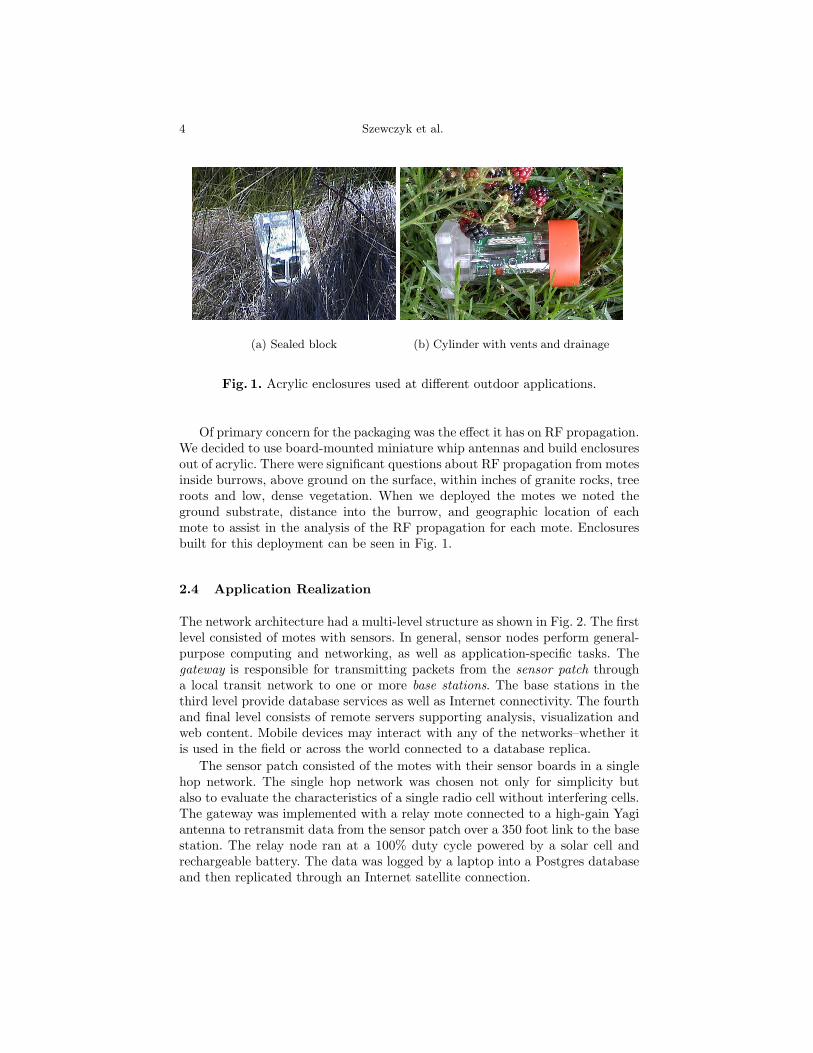
(a) Sealed block (b) Cylinder with vents and drainage

Fig. 1. Acrylic enclosures used at different outdoor applications.

Of primary concern for the packaging was the effect it has on RF propagation.We decided to use board-mounted miniature whip antennas and build enclosuresout of acrylic. There were significant questions about RF propagation from motesinside burrows, above ground on the surface, within inches of granite rocks, treeroots and low, dense vegetation. When we deployed the motes we noted theground substrate, distance into the burrow, and geographic location of eachmote to assist in the analysis of the RF propagation for each mote. Enclosuresbuilt for this deployment can be seen in Fig. 1.

2.4 Application Realization

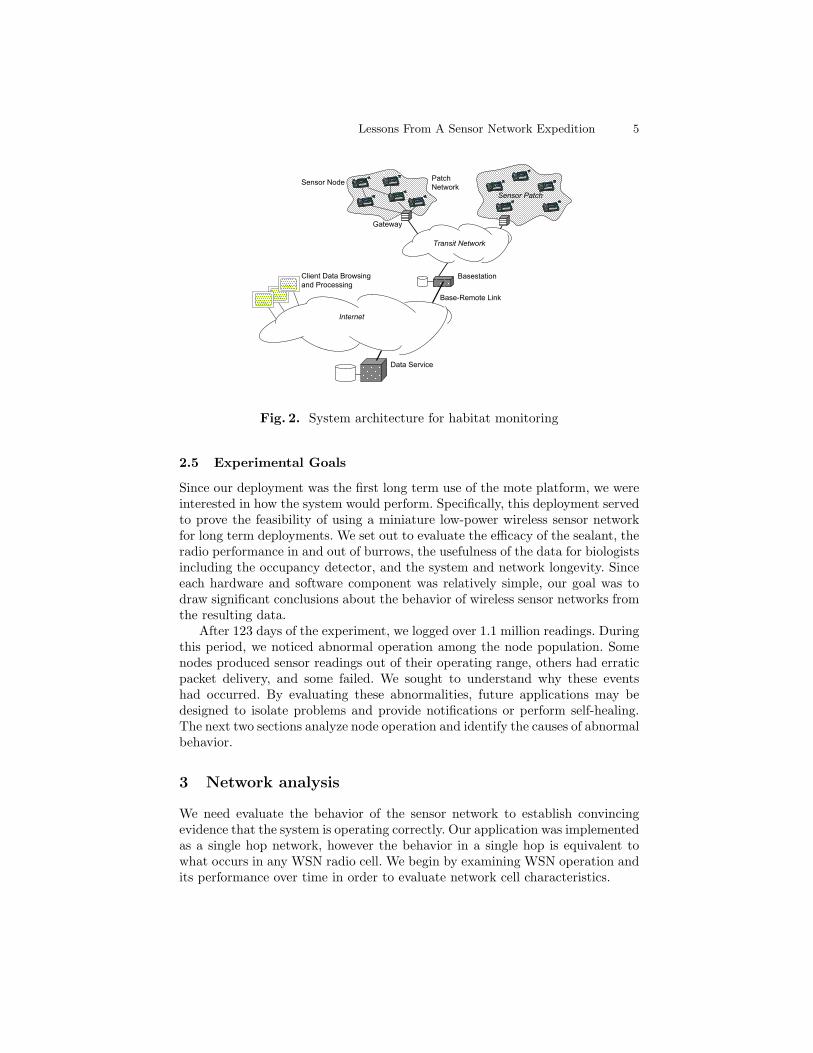
The network architecture had a multi-level structure as shown in Fig. 2. The firstlevel consisted of motes with sensors. In general, sensor nodes perform general-purpose computing and networking, as well as application-specific tasks. Thegateway is responsible for transmitting packets from the sensor patch througha local transit network to one or more base stations. The base stations in thethird level provide database services as well as Internet connectivity. The fourthand final level consists of remote servers supporting analysis, visualization andweb content. Mobile devices may interact with any of the networks–whether itis used in the field or across the world connected to a database replica.

The sensor patch consisted of the motes with their sensor boards in a singlehop network. The single hop network was chosen not only for simplicity butalso to evaluate the characteristics of a single radio cell without interfering cells.The gateway was implemented with a relay mote connected to a high-gain Yagiantenna to retransmit data from the sensor patch over a 350 foot link to the basestation. The relay node ran at a 100% duty cycle powered by a solar cell andrechargeable battery. The data was logged by a laptop into a Postgres databaseand then replicated through an Internet satellite connection.

Lessons From A Sensor Network Expedition 5

Transit Network

Basestation

Gateway

Sensor Patch

Patch Network

Base-Remote Link

Data Service

Internet

Client Data Browsingand Processing

Sensor Node

Fig. 2. System architecture for habitat monitoring

2.5 Experimental Goals

Since our deployment was the first long term use of the mote platform, we wereinterested in how the system would perform. Specifically, this deployment servedto prove the feasibility of using a miniature low-power wireless sensor networkfor long term deployments. We set out to evaluate the efficacy of the sealant, theradio performance in and out of burrows, the usefulness of the data for biologistsincluding the occupancy detector, and the system and network longevity. Sinceeach hardware and software component was relatively simple, our goal was todraw significant conclusions about the behavior of wireless sensor networks fromthe resulting data.

After 123 days of the experiment, we logged over 1.1 million readings. Duringthis period, we noticed abnormal operation among the node population. Somenodes produced sensor readings out of their operating range, others had erraticpacket delivery, and some failed. We sought to understand why these eventshad occurred. By evaluating these abnormalities, future applications may bedesigned to isolate problems and provide notifications or perform self-healing.The next two sections analyze node operation and identify the causes of abnormalbehavior.

3 Network analysis

We need evaluate the behavior of the sensor network to establish convincingevidence that the system is operating correctly. Our application was implementedas a single hop network, however the behavior in a single hop is equivalent towhat occurs in any WSN radio cell. We begin by examining WSN operation andits performance over time in order to evaluate network cell characteristics.

6 Szewczyk et al.

Jul Aug Sep Oct Nov Dec0

102030405060708090

100

Mea

n pa

cket

del

iver

y ra

te (%

)

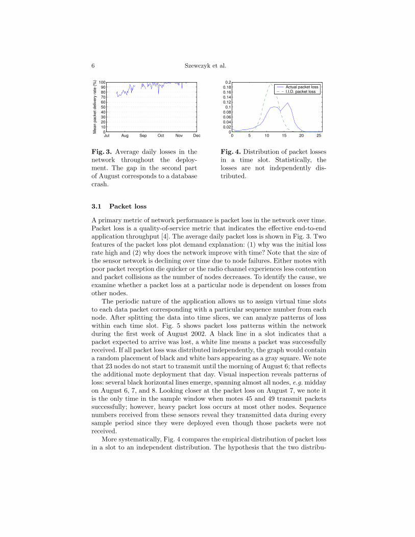
Fig. 3. Average daily losses in thenetwork throughout the deploy-ment. The gap in the second partof August corresponds to a databasecrash.

0 5 10 15 20 250

0.020.040.060.08

0.10.120.140.160.18

0.2

Missing packets per time slot

Actual packet lossI.I.D. packet loss

Fig. 4. Distribution of packet lossesin a time slot. Statistically, thelosses are not independently dis-tributed.

3.1 Packet loss

A primary metric of network performance is packet loss in the network over time.Packet loss is a quality-of-service metric that indicates the effective end-to-endapplication throughput [4]. The average daily packet loss is shown in Fig. 3. Twofeatures of the packet loss plot demand explanation: (1) why was the initial lossrate high and (2) why does the network improve with time? Note that the size ofthe sensor network is declining over time due to node failures. Either motes withpoor packet reception die quicker or the radio channel experiences less contentionand packet collisions as the number of nodes decreases. To identify the cause, weexamine whether a packet loss at a particular node is dependent on losses fromother nodes.

The periodic nature of the application allows us to assign virtual time slotsto each data packet corresponding with a particular sequence number from eachnode. After splitting the data into time slices, we can analyze patterns of losswithin each time slot. Fig. 5 shows packet loss patterns within the networkduring the first week of August 2002. A black line in a slot indicates that apacket expected to arrive was lost, a white line means a packet was successfullyreceived. If all packet loss was distributed independently, the graph would containa random placement of black and white bars appearing as a gray square. We notethat 23 nodes do not start to transmit until the morning of August 6; that reflectsthe additional mote deployment that day. Visual inspection reveals patterns ofloss: several black horizontal lines emerge, spanning almost all nodes, e.g. middayon August 6, 7, and 8. Looking closer at the packet loss on August 7, we note itis the only time in the sample window when motes 45 and 49 transmit packetssuccessfully; however, heavy packet loss occurs at most other nodes. Sequencenumbers received from these sensors reveal they transmitted data during everysample period since they were deployed even though those packets were notreceived.

More systematically, Fig. 4 compares the empirical distribution of packet lossin a slot to an independent distribution. The hypothesis that the two distribu-

Lessons From A Sensor Network Expedition 7

Mote ID

Dat

e

1 2 3 4 9 10 12 13 15 16 17 18 19 22 24 25 29 30 32 35 38 39 41 42 43 45 46 48 49 50 51 52 54 55 57 58 59 90

08/05

08/06

08/07

08/08

08/09

08/10

08/11

Fig. 5. Packet loss patterns within the deployed network during a week in Au-gust. Y-axis represents time divided into virtual packet slots (note: time increasesdownwards). A black line in the slot indicates that a packet expected to arrivein this time slot was missed, a white line means that a packet was successfullyreceived.

tions are the same is rejected by both parametric (χ2 test yields 108) and non-parametric techniques (rank test rejects it with 99% confidence). The empiricaldistribution appears a superposition of two Gaussians: this is not particularlysurprising, since we record packet loss at the end of the path (recall networkarchitecture, Section 2). This loss is a combination of potential losses along twohops in the network. Additionally, packets share the channel that varies withthe environmental conditions, and sensor nodes are likely to have similar bat-tery levels. Finally, there is a possibility of packet collisions at the relay nodes.

3.2 Network dynamics

Given that the expected network utilization is very low (less than 5%) we wouldnot expect collisions to play a significant role. Conversely, the behavior of motes45 and 49 implies otherwise: their packets are only received when most packetsfrom other nodes are lost. Such behavior is possible in a periodic application: inthe absence of any backoff, the nodes will collide repeatedly. In our application,the backoff was provided by the CSMA MAC layer. If the MAC worked asexpected, each node would backoff until it found a clear slot; at that point, wewould expect the channel to be clear. Clock skew and channel variations mightforce a slot reallocation, but such behavior should be infrequent.

Looking at the timestamps of the received packets, we can compute the phaseof each node, relative to the 70 second sampling period. Fig. 6 plots the phase

8 Szewczyk et al.

08/06 08/07 08/08 08/09 08/10 08/11 08/120

10

20

30

40

50

60

70

Time (days)

Pha

se (s

econ

ds)

13151718494555

13 55

18

15 17

49

45

09:00 12:00 15:000

10

20

30

40

50

60

70

Time (hours)

Pha

se (s

econ

ds)

13151718494555

17

15

55

18

13

49

45

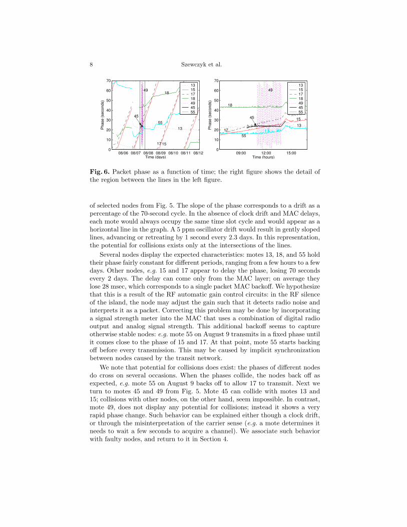
Fig. 6. Packet phase as a function of time; the right figure shows the detail ofthe region between the lines in the left figure.

of selected nodes from Fig. 5. The slope of the phase corresponds to a drift as apercentage of the 70-second cycle. In the absence of clock drift and MAC delays,each mote would always occupy the same time slot cycle and would appear as ahorizontal line in the graph. A 5 ppm oscillator drift would result in gently slopedlines, advancing or retreating by 1 second every 2.3 days. In this representation,the potential for collisions exists only at the intersections of the lines.

Several nodes display the expected characteristics: motes 13, 18, and 55 holdtheir phase fairly constant for different periods, ranging from a few hours to a fewdays. Other nodes, e.g. 15 and 17 appear to delay the phase, losing 70 secondsevery 2 days. The delay can come only from the MAC layer; on average theylose 28 msec, which corresponds to a single packet MAC backoff. We hypothesizethat this is a result of the RF automatic gain control circuits: in the RF silenceof the island, the node may adjust the gain such that it detects radio noise andinterprets it as a packet. Correcting this problem may be done by incorporatinga signal strength meter into the MAC that uses a combination of digital radiooutput and analog signal strength. This additional backoff seems to captureotherwise stable nodes: e.g. mote 55 on August 9 transmits in a fixed phase untilit comes close to the phase of 15 and 17. At that point, mote 55 starts backingoff before every transmission. This may be caused by implicit synchronizationbetween nodes caused by the transit network.

We note that potential for collisions does exist: the phases of different nodesdo cross on several occasions. When the phases collide, the nodes back off asexpected, e.g. mote 55 on August 9 backs off to allow 17 to transmit. Next weturn to motes 45 and 49 from Fig. 5. Mote 45 can collide with motes 13 and15; collisions with other nodes, on the other hand, seem impossible. In contrast,mote 49, does not display any potential for collisions; instead it shows a veryrapid phase change. Such behavior can be explained either though a clock drift,or through the misinterpretation of the carrier sense (e.g. a mote determines itneeds to wait a few seconds to acquire a channel). We associate such behaviorwith faulty nodes, and return to it in Section 4.

Lessons From A Sensor Network Expedition 9

4 Node-level analysis

Nodes in outdoor WSNs are exposed to closely monitor and sense their environ-ment. Their performance and reliability depend on a number of environmentalfactors. Fortunately, the nodes have a local knowledge of these factors, and theymay exploit that knowledge to adjust their operation. Appropriate notificationsfrom the system would allow the end user to pro-actively fix the WSN. Ideally,the network could request proactive maintenance, or self-heal. We examine thelink between sensor and node performance. Although the particular analysis isspecific to this deployment, we believe that other systems will be benefit fromsimilar analyses: identifying outlier readings or loss of expected sensing pat-terns, across time, space or sensing modality. Additionally, since battery stateis an important part of a node’s self-monitoring capability [26], we also examinebattery voltage readings to analyze the performance of our power managementimplementation.

4.1 Sensor analysis

The suite of sensors on each node provided analog light, humidity, digital temper-ature, pressure, and passive infrared readings. The sensor board used a separate12-bit ADC to maximize the resolution and minimize analog noise. We examinethe readings from each sensor.

Light readings: The light sensor used for this application was a photoresis-tor that we had significant experience with in the past. It served as a confidencebuilding tool and ADC test. In an outdoor setting during the day, the light valuesaturated at the maximum ADC value, and at night the values were zero. Know-ing the saturation characteristics, not much work was invested in characterizingits response to known intensities of light. The simplicity of this sensor combinedwith an a priori knowledge of the expected response provided a valuable base-line for establishing the proper functioning of the sensor board. As expected,the sensors deployed above ground showed periodic patterns of day and nightand burrows showed near to total darkness. Fig. 7 shows light and temperaturereadings and average light and temperature readings during the experiment.

The light sensor operated most reliably of the sensors. The only behavioridentifiable as failure was disappearance of diurnal patterns replaced by highvalue readings. Such behavior is observed in 7 nodes out of 43, and in 6 casesit is accompanied by anomalous readings from other sensors, such as a 0oCtemperature or analog humidity values of zero.

Temperature readings: A Maxim 6633 digital temperature sensor providedthe temperature measurements While the sensor’s resolution is 0.0625oC, in ourdeployment it only provided a 2oC resolution: the hardware always suppliedreadings with the low-order bits zeroed out. The enclosure was IR transpar-ent to assist the thermopile sensor; consequently, the IR radiation from directsunlight would enter the enclosure and heat up the mote. As a result, tempera-tures measured inside the enclosures were significantly higher than the ambient

10 Szewczyk et al.

07/21 07/22 07/23 07/24 07/25 07/26 07/27 07/28 07/29

0

10

20

30

40

50

60

70

80

90

100Light Level (%)Temperature (oC)

07/21 07/22 07/23 07/24 07/25 07/26

0

10

20

30

40

50

60

70

80

90

100Light Level (%)Temperature (oC)

Jul Aug Sep Oct Nov Dec

0

10

20

30

40

50

60

70

80

90

100Light Level (%)Temperature (oC)

Fig. 7. Light and temperature time series from the network. From left: outside,inside, and daily average outside burrows.

temperatures measured by traditional weather stations. On cloudy days the tem-perature readings corresponded closely with the data from nearby weather buoysoperated by NOAA.

Even though motes were coated with parylene, sensor elements were leftexposed to the environment to preserve their sensing ability. In the case of thetemperature sensor, a layer of parylene was permissible. Nevertheless the sensorfailed when it came in direct contact with water. The failure manifested itself in apersistent reading of 0oC. Of 43 nodes, 22 recorded a faulty temperature readingand 14 of those recorded their first bad reading during storms on August 6. Thefailure of temperature sensor is highly correlated with the failure of the humiditysensor: of 22 failure events, in two cases the humidity sensor failed first and intwo cases the temperature sensor failed first. In remaining 18 cases, the twosensors failed simultaneously. In all but two cases, the sensor did not recover.

Humidity readings: The relative humidity sensor was a capacitive sensor: itscapacitance was proportional to the humidity. In the packaging process, thesensor needed to be exposed; it was masked out during the parylene sealing pro-cess, and we relied on the enclosure to provide adequate air circulation whilekeeping the sensor dry. Our measurements have shown up to 15% error in theinterchangeability of this sensor across sensor boards. Tests in a controlled en-vironment have shown the sensor produces readings with 5% variation due toanalog noise. Prior to deployment, we did not perform individual calibration;instead we applied the reference conversion function to convert the readings intoSI units.

In the field, the protection afforded by our enclosure proved to be inadequate.When wet, the sensor would create a low-resistance path between the powersupply terminals. Such behavior would manifest itself in either abnormally large(more than 150%) or very small humidity readings (raw readings of 0V). Fig. 8shows the humidity and voltage readings as well as the packet reception rates ofselected nodes during both rainy and dry days in early August. Nodes 17 and 29experienced a large drop in voltage while recording an abnormally high humidityreadings on Aug. 5 and 6. We attribute the voltage drop to excessive load on thebatteries caused by the wet sensor. Node 18 shows an more severe effect of rain:on Aug. 5, it crashes just as the other sensors register a rise in the humidity

Lessons From A Sensor Network Expedition 11

08/05 08/06 08/07 08/08 08/09 08/10 08/110

100

200

Hum

idity

(%)

08/05 08/06 08/07 08/08 08/09 08/10 08/110

2

Vol

tage

(V)

08/05 08/06 08/07 08/08 08/09 08/10 08/110

50

Pac

kets

rece

ived

per h

our 17

182955

17182955

17182955

Node 18: extended down−time,followed by self−recovery

Fig. 8. Sensor behavior during the rain. Nodes 17 and 29 experience substantialdrop in voltage, while node 55 crashes. When the humidity sensor recovers, thenodes recover.

readings. Node 18, on the other hand, seems to be well protected: it registershigh humidity readings on Aug. 6, and its voltage and packet delivery ratesare not correlated with the humidity readings. Nodes that experienced the highhumidity readings typically recover when they dried up; nodes with the unusuallylow readings would fail quickly. While we do not have a definite explanation forsuch behavior, we evaluate that characteristics of the sensor board as a failureindicator below.

Thermopile readings: The data from the thermopile sensor proved difficult toanalyze. The sensor measures two quantities: the ambient temperature and theinfrared radiation incident on the element. The sum of thermopile and thermistorreadings yields the object surface temperature, e.g. a bird. We would expect thatthe temperature readings from the thermistor and from the infrared temperaturesensor would closely track each other most of the time. By analyzing spikes inthe IR readings, we should be able to deduce the bird activity.

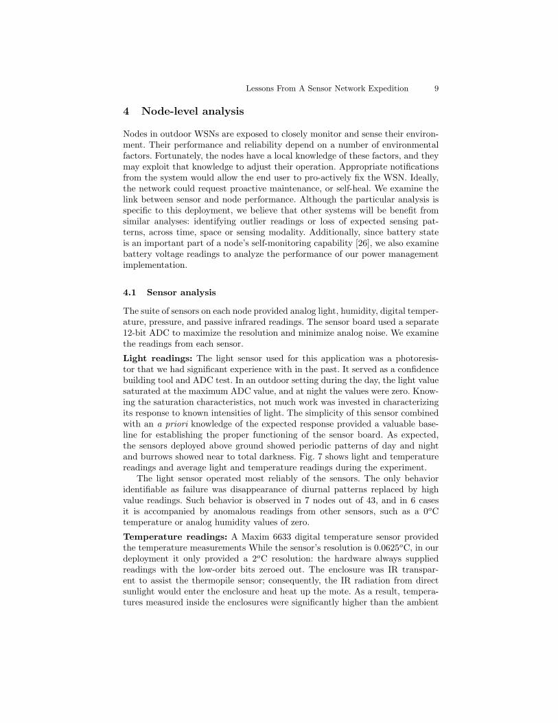
The readings from the thermistor do, in fact, track closely with the temper-ature readings. Fig. 9 compares the analog thermistor with the digital maximtemperature sensor. The readings are closely correlated although different onan absolute scale. A best linear fit of the temperature data to the thermistorreadings on a per sensor per day basis yields a mean error of less than 0.9oC,within the half step resolution of the digital sensor. The best fit coefficient variessubstantially across the nodes.

Assigning biological significance to the infrared data is a difficult task. Theabsolute readings often do not fall in the expected range. The data exhibits a lackof any periodic daily patterns (assuming that burrow occupancy would exhibitthem), and the sensor output appears to settle quickly in one of the two extremereadings. In the absence of any ground truth information, e.g. infrared cameraimages corresponding to the changes in the IR reading, the data is inconclusive.

12 Szewczyk et al.

07/21 07/22 07/23 07/24 07/25 07/26 07/27 07/28 07/2910

12

14

16

18

Tem

pera

ture

(o C)

07/21 07/22 07/23 07/24 07/25 07/26 07/27 07/28 07/29−28−26−24−22−20−18

Unc

orre

cted

The

rmis

tor (

o C)

Fig. 9. The temperature sensor(top) and thermistor (bottom),though very different on the abso-lute scale, are closely correlated: alinear fit yields a mean error of lessthan 0.8oC.

07/18 07/28 08/07 08/17 08/27 09/06 09/160

0.5

1

1.5

2

2.5

3

Average daily voltage at node 57

Time

Vol

tage

(V)

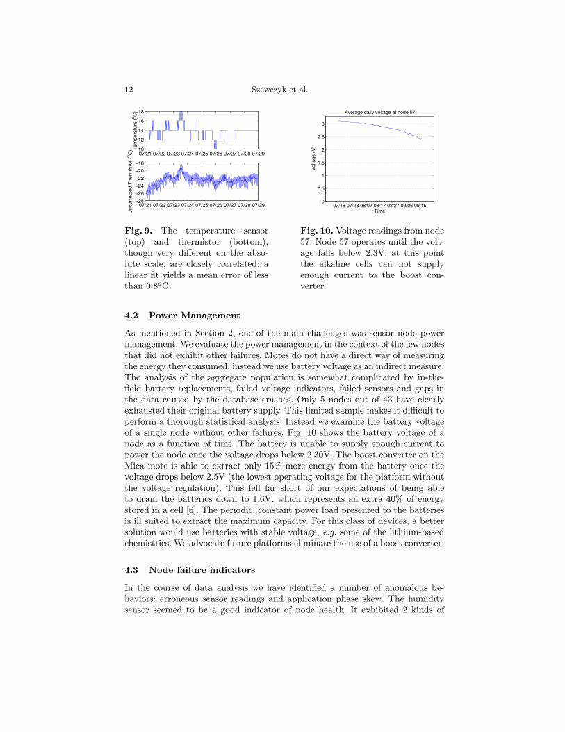
Fig. 10. Voltage readings from node57. Node 57 operates until the volt-age falls below 2.3V; at this pointthe alkaline cells can not supplyenough current to the boost con-verter.

4.2 Power Management

As mentioned in Section 2, one of the main challenges was sensor node powermanagement. We evaluate the power management in the context of the few nodesthat did not exhibit other failures. Motes do not have a direct way of measuringthe energy they consumed, instead we use battery voltage as an indirect measure.The analysis of the aggregate population is somewhat complicated by in-the-field battery replacements, failed voltage indicators, failed sensors and gaps inthe data caused by the database crashes. Only 5 nodes out of 43 have clearlyexhausted their original battery supply. This limited sample makes it difficult toperform a thorough statistical analysis. Instead we examine the battery voltageof a single node without other failures. Fig. 10 shows the battery voltage of anode as a function of time. The battery is unable to supply enough current topower the node once the voltage drops below 2.30V. The boost converter on theMica mote is able to extract only 15% more energy from the battery once thevoltage drops below 2.5V (the lowest operating voltage for the platform withoutthe voltage regulation). This fell far short of our expectations of being ableto drain the batteries down to 1.6V, which represents an extra 40% of energystored in a cell [6]. The periodic, constant power load presented to the batteriesis ill suited to extract the maximum capacity. For this class of devices, a bettersolution would use batteries with stable voltage, e.g. some of the lithium-basedchemistries. We advocate future platforms eliminate the use of a boost converter.

4.3 Node failure indicators

In the course of data analysis we have identified a number of anomalous be-haviors: erroneous sensor readings and application phase skew. The humiditysensor seemed to be a good indicator of node health. It exhibited 2 kinds of

Lessons From A Sensor Network Expedition 13

0 10 20 30 40 50 60 700

0.1

0.2

0.3

0.4

0.5

0.6

0.7

0.8

0.9

1

Time (days)

Pro

babi

lity

of fa

ilure

Relative humidityClock skewCombinationTotal population

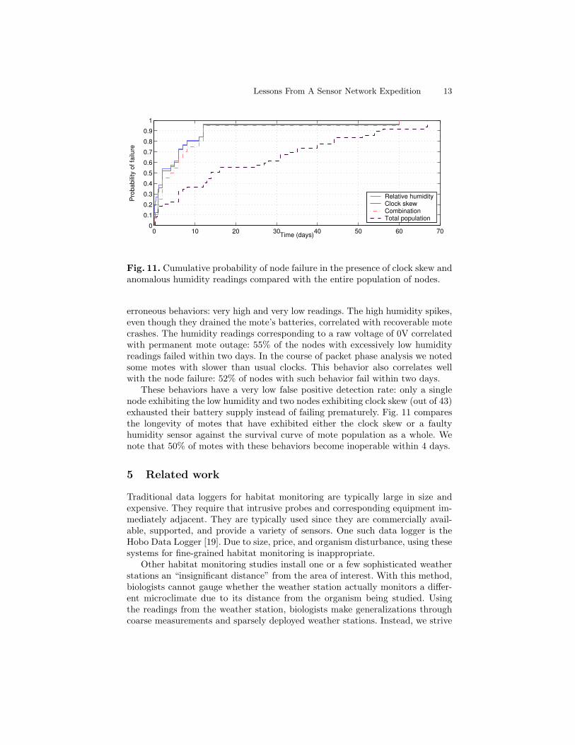
Fig. 11. Cumulative probability of node failure in the presence of clock skew andanomalous humidity readings compared with the entire population of nodes.

erroneous behaviors: very high and very low readings. The high humidity spikes,even though they drained the mote’s batteries, correlated with recoverable motecrashes. The humidity readings corresponding to a raw voltage of 0V correlatedwith permanent mote outage: 55% of the nodes with excessively low humidityreadings failed within two days. In the course of packet phase analysis we notedsome motes with slower than usual clocks. This behavior also correlates wellwith the node failure: 52% of nodes with such behavior fail within two days.

These behaviors have a very low false positive detection rate: only a singlenode exhibiting the low humidity and two nodes exhibiting clock skew (out of 43)exhausted their battery supply instead of failing prematurely. Fig. 11 comparesthe longevity of motes that have exhibited either the clock skew or a faultyhumidity sensor against the survival curve of mote population as a whole. Wenote that 50% of motes with these behaviors become inoperable within 4 days.

5 Related work

Traditional data loggers for habitat monitoring are typically large in size andexpensive. They require that intrusive probes and corresponding equipment im-mediately adjacent. They are typically used since they are commercially avail-able, supported, and provide a variety of sensors. One such data logger is theHobo Data Logger [19]. Due to size, price, and organism disturbance, using thesesystems for fine-grained habitat monitoring is inappropriate.

Other habitat monitoring studies install one or a few sophisticated weatherstations an “insignificant distance” from the area of interest. With this method,biologists cannot gauge whether the weather station actually monitors a differ-ent microclimate due to its distance from the organism being studied. Usingthe readings from the weather station, biologists make generalizations throughcoarse measurements and sparsely deployed weather stations. Instead, we strive

14 Szewczyk et al.

to provide biologists the ability to monitor the environment on the scale of theorganism, not on the scale of the biologist [8,21].

Habitat monitoring for WSNs has been studied by a variety of other researchgroups. Cerpa et. al. [3] propose a multi-tiered architecture for habitat moni-toring. The architecture focuses primarily on wildlife tracking instead of habitatmonitoring. A PC104 hardware platform was used for the implementation withfuture work involving porting the software to motes. Experimentation using ahybrid PC104 and mote network has been done to analyze acoustic signals [23],but no long term results or reliability data has been published. Wang et. al. [22]implement a method to acoustically identify animals using a hybrid iPaq andmote network.

ZebraNet [14] is a WSN for monitoring and tracking wildlife. ZebraNet nodesare significantly larger and heavier than motes. The architecture is designed foran always mobile, multi-hop wireless network. In many respects, this design doesnot fit with monitoring the Leach’s Storm Petrel at static positions (burrows).ZebraNet, at the time of this writing, has not yet had a full long-term deploy-ment.

The number of deployed wireless sensor network systems is extremely low.The Center for Embedded Network Sensing (CENS) has deployed their Exten-sible Sensing System [7] at the James Mountain Reserve in California. Theirarchitecture is similar to ours with a variety of sensor patches connected via atransit network that is tiered. Intel Research has recently deployed a networkto monitor Redwood canopies in Northern California and a second network tomonitor vineyards in Oregon. We deployed a second generation multihop habi-tat monitoring network on Great Duck Island, Maine in the summer of 2003.These networks are in their infancy but analysis may yield the benefits of variousapproaches to deploying habitat monitoring systems.

6 Conclusion

We have analyzed the environmental data from one of the first outdoor deploy-ments of WSNs. While the deployment exhibited very high node failure rates, ityielded valuable insight into WSN operation that could not have been obtainedin simulation or in an indoor deployment. We have identified sensor featuresthat predict a 50% node failure within 4 days. We analyzed the application-leveldata to show complex behaviors in low levels of the system, such as MAC-layersynchronization of nodes. We have shown that great care must be taken whendeploying WSNs such that the MAC implementation, network topology, syn-chronization, sensing modalities, sensor design, and packaging be designed withawareness of each other.

Sensor networks do not exist in isolation from their environment; they areembedded within it and greatly affected by it. This work shows that the anoma-lies in sensor readings can predict node failures with high confidence. Predictionenables pro-active maintenance and node self-maintenance. This insight will bevery important in the development of self-organizing and self-healing WSNs.

Lessons From A Sensor Network Expedition 15

Notes

Data from the wireless sensor network deployment on Great Duck Island canbe view graphically at http://www.greatduckisland.net. Our website alsoincludes the raw data for researchers in both computer science and the biologicalsciences to download and analyze.

This work was supported by the Intel Research Laboratory at Berkeley,DARPA grant F33615-01-C1895 (Network Embedded Systems Technology), theNational Science Foundation, and the Center for Information Technology Re-search in the Interest of Society (CITRIS).

References

1. Bulusu, N., Bychkovskiy, V., Estrin, D., and Heidemann, J. Scalable, ad hocdeployable, RF-based localization. In Proceedings of the Grace Hopper Conferenceon Celebration of Women in Computing (Vancouver, Canada, Oct. 2002).

2. Bychkovskiy, V., Megerian, S., Estrin, D., and Potkonjak, M. Colibration:A collaborative approach to in-place sensor calibration. In Proceedings of the 2ndInternational Workshop on Information Processing in Sensor Networks (IPSN’03)(Palo Alto, CA, USA, Apr. 2003).

3. Cerpa, A., Elson, J., Estrin, D., Girod, L., Hamilton, M., and Zhao, J.Habitat monitoring: Application driver for wireless communications technology. In2001 ACM SIGCOMM Workshop on Data Communications in Latin America andthe Caribbean (San Jose, Costa Rica, Apr. 2001).

4. Chalmers, D., and Sloman, M. A survey of Quality of Service in mobile com-puting environments. IEEE Communications Surveys 2, 2 (1992).

5. Chen, B., Jamieson, K., Balakrishnan, H., and Morris, R. Span: An energy-efficient coordination algorithm for topology maintenance in ad hoc wireless net-works. In Proceedings of the 7th Annual International Conference on Mobile Com-puting and Networking (Rome, Italy, July 2001), ACM Press, pp. 85–96.

6. Eveready Battery Company. Energizer no. x91 datasheet. http:

//data.energizer.com/datasheets/library/primary/alkaline/energizer_

e2/x91.pdf.7. Hamilton, M., Allen, M., Estrin, D., Rottenberry, J., Rundel, P., Sri-

vastava, M., and Soatto, S. Extensible sensing system: An advanced networkdesign for microclimate sensing. http://www.cens.ucla.edu, June 2003.

8. Happold, D. C. The subalpine climate at smiggin holes, Kosciusko NationalPark, Australia, and its influence on the biology of small mammals. Arctic &Alpine Research 30 (1998), 241–251.

9. He, T., Blum, B., Stankovic, J., and Abdelzaher, T. AIDA: Adaptive Appli-cation Independant Data Aggregation in Wireless Sensor Networks. ACM Trans-actions in Embedded Computing Systems (TECS), Special issue on DynamicallyAdaptable Embedded Systems (2003).

10. Hill, J., and Culler, D. Mica: a wireless platform for deeply embedded networks.IEEE Micro 22, 6 (November/December 2002), 12–24.

11. Hill, J., Szewczyk, R., Woo, A., Hollar, S., Culler, D., and Pister, K.System architecture directions for networked sensors. In Proceedings of the 9thInternational Conference on Architectural Support for Programming Languages andOperating Systems (ASPLOS-IX) (Cambridge, MA, USA, Nov. 2000), ACM Press,pp. 93–104.

16 Szewczyk et al.

12. Huntington, C., Butler, R., and Mauck, R. Leach’s Storm Petrel (Ocean-odroma leucorhoa), vol. 233 of Birds of North America. The Academy of NaturalSciences, Philadelphia and the American Orinthologist’s Union, Washington D.C.,1996.

13. Intanagonwiwat, C., Govindan, R., and Estrin, D. Directed diffusion: ascalable and robust communication paradigm for sensor networks. In Proceedingsof the 6th Annual International Conference on Mobile Computing and Networking(Boston, MA, USA, Aug. 2000), ACM Press, pp. 56–67.

14. Juang, P., Oki, H., Wang, Y., Martonosi, M., Peh, L.-S., and Ruben-stein, D. Energy-efficient computing for wildlife tracking: Design tradeoffs andearly experiences with ZebraNet. In Proceedings of the 10th International Confer-ence on Architectural Support for Programming Languages and Operating Systems(ASPLOS-X) (San Jose, CA, USA, Oct. 2002), ACM Press, pp. 96–107.

15. Krishanamachari, B., Estrin, D., and Wicker, S. The impact of data aggre-gation in wireless sensor networks. In Proceedings of International Workshop ofDistributed Event Based Systems (DEBS) (Vienna, Austria, July 2002).

16. Liu, J., Cheung, P., Guibas, L., and Zhao, F. A dual-space approach totracking and sensor management in wireless sensor networks. In Proceedings of the1st ACM International Workshop on Wireless Sensor Networks and Applications(Atlanta, GA, USA, Sept. 2002), ACM Press, pp. 131–139.

17. Madden, S., Franklin, M., Hellerstein, J., and Hong, W. TAG: a TinyAGgregation service for ad-hoc sensor networks. In Proceedings of the 5th USENIXSymposium on Operating Systems Design and Implementation (OSDI ’02) (Boston,MA, USA, Dec. 2002).

18. Mainwaring, A., Polastre, J., Szewczyk, R., Culler, D., and Anderson,J. Wireless sensor networks for habitat monitoring. In Proceedings of the 1st ACMInternational Workshop on Wireless Sensor Networks and Applications (Atlanta,GA, USA, Sept. 2002), ACM Press, pp. 88–97.

19. Onset Computer Corporation. HOBO weather station. http://www.

onsetcomp.com.20. Polastre, J. Design and implementation of wireless sensor networks for habitat

monitoring. Master’s thesis, University of California at Berkeley, 2003.21. Toapanta, M., Funderburk, J., and Chellemi, D. Development of Franklin-

iella species (Thysanoptera: Thripidae) in relation to microclimatic temperaturesin vetch. Journal of Entomological Science 36 (2001), 426–437.

22. Wang, H., Elson, J., Girod, L., Estrin, D., and Yao, K. Target classificationand localization in habitat monitoring. In Proceedings of IEEE International Con-ference on Acoustics, Speech, and Signal Processing (ICASSP 2003) (Hong Kong,China, Apr. 2003).

23. Wang, H., Estrin, D., and Girod, L. Preprocessing in a tiered sensor networkfor habitat monitoring. EURASIP JASP Special Issue on Sensor Networks 2003,4 (Mar. 2003), 392–401.

24. Whitehouse, K., and Culler, D. Calibration as parameter estimation in sensornetworks. In Proceedings of the 1st ACM International Workshop on WirelessSensor Networks and Applications (Atlanta, GA, USA, Sept. 2002), ACM Press.

25. Xu, Y., Heidemann, J., and Estrin, D. Geography-informed energy conserva-tion for ad hoc routing. In Proceedings of the 7th Annual International Conferenceon Mobile Computing and Networking (Rome, Italy, July 2001), ACM Press.

26. Zhao, J., Govindan, R., and Estrin, D. Computing aggregates for monitoringwireless sensor networks. In Proceedings of the 1st IEEE International Workshopon Sensor Network Protocols and Applications (Anchorage, AK, USA, May 2003).