Lesson 6: Computer method overviewLesson 6: Computer method overview

Neutron transport overviews Comparison of deterministic vs. Monte Carlo

User-level knowledge of Monte Carlo Example calc: Approach to critical

Neutron transport overview

Neutron balance equationNeutron balance equation

Scalar flux/current balance

Used in shielding, reactor theory, crit. safety, kinetics

Problem: No source=No solution !

ErSErErErErErJ fa ,,,,,,

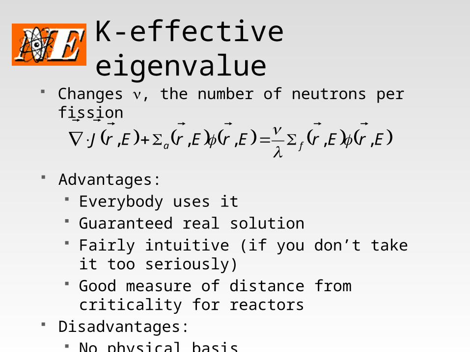
K-effective eigenvalueK-effective eigenvalue Changes n, the number of neutrons per fission

ErErErErErJ fa ,,,,,

Advantages: Everybody uses it Guaranteed real solution Fairly intuitive (if you don’t take it too seriously) Good measure of distance from criticality for reactors

Disadvantages: No physical basis Not a good measure of distance from criticality for CS

Neutron transportNeutron transport Scalar vs. angular flux Boltzmann transport equation

Neutron accounting balance General terms of a balance in energy, angle, space

Deterministic Subdivide energy, angle, space and solve equation Get k-effective and flux

Monte Carlo Numerical simulation of transport Get particular flux-related answers, not flux

everywhere

Deterministic grid solutionDeterministic grid solution

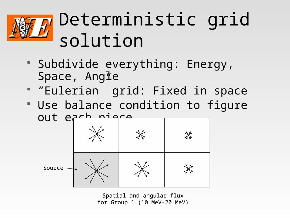
Subdivide everything: Energy, Space, Angle “Eulerian” grid: Fixed in space Use balance condition to figure out each piece

Spatial and angular flux for Group 1 (10 MeV-20 MeV)

Source

Stochastic solutionStochastic solution

Continuous in Energy, Space, Angle “Lagrangian” grid: Follows the particle Sample (poll) by following “typical” neutrons

Particle track of two 10 MeV fission neutrons

Fissile

Absorbed

Fission

Advantages and disadvantages of eachAdvantages and disadvantages of each

Advantages Disadvantages

DiscreteOrdinates(deterministic)

Fast (1D, 2D) Accurate for simple geometries Delivers answer everywhere: = Complete spatial, energy, angular map of the flux 1/N (or better) error convergence

Slow (3D) Multigroup energy required Geometry must be approximated Large computer memory requirements User must determine accuracy by repeated calculations

Monte Carlo(stochastic)

“Exact” geometry Continuous energy possible Estimate of accuracy given

Slow (1,2,3D) Large computer time requirements 1/N1/2 error convergence

Monte Carlo overview

Monte CarloMonte Carlo

We will cover the mathematical details in 3 steps

1. General overview of MC approach2. Example walkthrough3. Special considerations for criticality

calculations Goal: Give you just enough details for you

to be an intelligent user

General Overview of MCGeneral Overview of MC

Monte Carlo: Stochastic approach Statistical simulation of individual particle

histories Keep score of quantities you care about Most of mathematically interesting features

come from “variance reduction methods” Gives results PLUS standard deviation =

statistical measure of how reliable the answer is

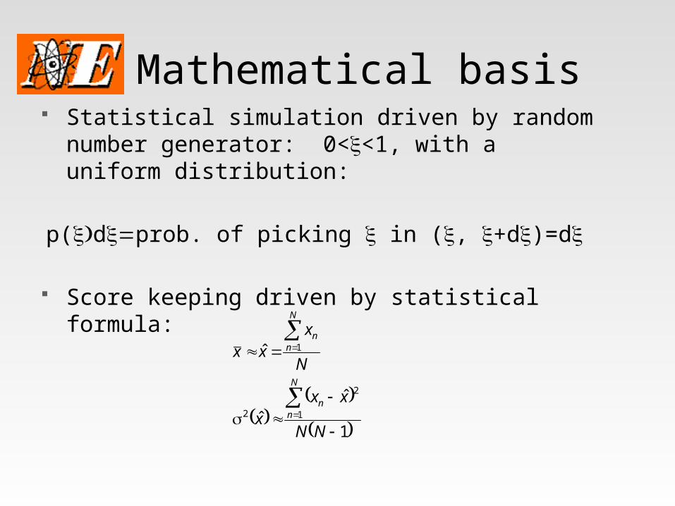
Mathematical basisMathematical basis Statistical simulation driven by random number generator:

0<x<1, with a uniform distribution:

p( )x d =x prob. of picking x in (x, x+dx)=dx

Score keeping driven by statistical formula:

1

ˆˆ

ˆ

1

2

2

1

NN

xxx

N

xxx

N

nn

N

nn

Simple Walkthrough Simple Walkthrough

Six types of decisions to be made:1. Where the particle is born2. Initial particle energy3. Initial particle direction4. Distance to next collision5. Type of collision6. Outcome of scattering collision (E, direction)

How are these decisions made?

Decision 1: Where particle is bornDecision 1: Where particle is born

3 choices:1. Set of fixed points (first “generation” only)2. Uniformly distributed (first generation only)

KENO picks point in geometry

Rejected if not in fuel After first generation, previous generation’s

sites used to start new fissions

min max

min max min

min max min

min max min

, uniformly distributed

( )

( )

( )

x x x

x x x x

y y y y

z z z z

Decision 2: Initial particle energyDecision 2: Initial particle energy

From a fission neutron energy spectrum Complicated algorithms based on advanced

mathematical treatments Rejection method based on “bounding box”

idea

Decision 3: Initial particle directionDecision 3: Initial particle direction

Easy one for us because all fission is isotropic Must choose the “longitude” and “latitude” that

the particle would cross a unit sphere centered on original location

Mathematical results: m=cosine of angle from polar axis

F=azimuthal angle (longitude)

1-2

ddistributeuniformly ,11

2

ddistributeuniformly ,20

Decision 4: Distance to next collisionDecision 4: Distance to next collision

Let s=distance traveled in medium with St Prob. of colliding in ds at distance s

=(Prob. of surviving to s)x(Prob. of colliding in ds|survived to s)

=(e- St s)x(Sts)

Using methods from NE582, this results in:

t

s

ln

Decision 5: Type of collisionDecision 5: Type of collision

Most straight-forward of all because straight from cross sections: Ss / St =probability of scatter Sa / St =probability of absorption

Therefore, if x< Ss / St , it is a scatter Otherwise particle is absorbed (lost) “Weighting in lieu of absorption”=fancy term for

following the non-absorbing fraction of the particle

Decision 6: Outcome of scattering collisionDecision 6: Outcome of scattering collision

In simplest case (isotropic scattering), a combination of Decisions 3 and 5: “Decision 5-like” choice of new energy group

g' group tog group fromscatter ofy probabilit

gs

ggs

Decision 3 gets new direction In more complicated (normal) case, must deal with

the energy/direction couplings from elastic and inelastic scattering physics

Special considerations for criticality safetySpecial considerations for criticality safety

Must deal w/ “generations”=outer iteration Fix a fission source spatial shape Find new fission source shape and eigenvalue

User must specify # of generations AND # of histories per generation AND # of generation to “skip”

Skipped generations allow the original lousy spatial fission distribution to improve before we really start keeping “score”

KENO defaults: 203 generations of 1000 histories per generation, skipping first 3

Approach to critical

Approach to criticalApproach to critical

This is a brief overview of the basic techniques of running a critical experiment The very same techniques are used to bring a

reactor from shutdown state to an initial zero-power critical condition

The basic idea is to use the equations of subcritical multiplication to sneak up on the critical value of some parameter (i.e., one of the nine MAGICMERV parameters)

Approach to critical (cont’d)Approach to critical (cont’d) We begin with the basic definition of k-

effective (which we will call “k” in our equations) The ratio of fission neutrons produced in any

“generation” to those in the previous generation Actually, since the flux increases linearly with

fission rate (if you are careful) any flux-dependent parameter can be used in place of the fission neutron production

• We will use the response of an external detector In both practice and theory, there must be an

external neutron source to give the system something to multiply

Approach to critical (cont’d)Approach to critical (cont’d) If we assume an external source rate of S

neutrons/generation, we can see that:1. In the first generation, S neutrons will be

released. Since no fission has taken place yet, these will be the only neutrons in the system.

2. In the second generation, S new neutrons will be released and the previous generation’s S neutrons will cause kS(<S) new neutrons to give us a population of:

(1 )S k

Approach to critical (cont’d)Approach to critical (cont’d)

3. In the next generation, the same thing happens: S new neutrons will be released and the previous population is multiplied by k, giving us:

4. Following this through to an infinite series:

2(1 ) (1 )S k S k S k k

2 3(1 ...)1

SS k k k

k

Approach to critical (cont’d)Approach to critical (cont’d)5. The 1/(1-k) term is a MULTIPLIER of the

source. It appears from first glance that this equation can be used to find k, but it really can’t, because we never really know what the original k is.

6. But it CAN tell you is how much (relatively) closer your most recent change got you to k=1.

For example, if you make a change and your detector reading goes from 100 counts/sec to 200 counts/sec, you DO know that you went HALFWAY to k=1. But you can’t tell whether you went from k=.8 to .9 or (maybe) 0.96 to 0.98

Approach to critical (cont’d)Approach to critical (cont’d) This is useful because it tells you that ANOTHER

change of (about) the same magnitude would get you to critical.

7. Since criticality corresponds to the M=1/(1-k) term (the MULTIPLIER of the source) going infinite, we have found it is more useful to instead watch its inverse.

Criticality corresponds to 1/M going to 0.

(Inclass example as time allows)