lesson 13: box-jenkins modeling strategy for building arma ... · introduction in this lesson we...

Lesson 13: Box-Jenkins Modeling

Strategy for building ARMA models

Umberto Triacca

Facolta di Economia

Universita dell’Aquila

[email protected]

Umberto Triacca Lesson 13: Box-Jenkins Modeling Strategy for building ARMA

Introduction

In this lesson we present a method to construct anARMA(p, q) model.

The so-called Box-Jenkins Modeling Strategy.


Introduction

The Box-Jenkins approach to modeling ARMA(p, q) modelswas described in a highly influential book by statisticiansGeorge Box and Gwilym Jenkins in 1970.

⇓

Box, G.E.P. and G.M. Jenkins (1970) Time series analysis:

Forecasting and control, San Francisco: Holden-Day.


Introduction

The Box-Jenkins modelling procedure involved a preliminaryanalysis (Data Transformation) and an iterative three-stageprocess:

1 Model identification

2 Model estimation

3 Model checking


Introduction

Each stage concerns a question.

Preliminary analysis: Is the time series stationary?

1 Model identification: What class of models probablyproduced the (transformed) series?

2 Model estimation: What are the model parameters?

3 Model checking: Are the residuals from the estimatedmodel white noise?


The assumption of stationarity

The assumption that our time series is a realization of astationary process is clearly fundamental in time seriesanalysis.

The Box-Jenkins methodology requires that the ARMA(p, q)process to be used in describing the DGP to be bothstationary and invertible.

Thus, in order to construct an ARMA model, we must firstdetermine whether our time series can be considered arealization of a stationary process.

If it is not, we must transform the time series in order to getthe stationarity.


The assumption of stationarity

A time series can be considered a realization of a stationarystochastic process if:

1 if there is no systematic change in mean (no trend),

2 if there is no systematic change in variance,

3 if there is no periodic variation.


Data Transformation

In this stage a very useful tool is the graph of the series.

From the plot of the time series values we can obtain usefulindications concerning the stationarity of the process.

If the observed values of the time series seem to fluctuate withconstant variation around a constant mean, then it isreasonable to suppose that the process is stationary, otherwise,it is nonstationary.


Time series

Figure : Time plot of a series generated by a stationary ARMAprocess.


Time series

In the practice many time series cannot be considered likerealizations of stationary processes.


Time series

Consider an example the Airline series.

Figure : Monthly totals in thousands of international airlinepassengers from January 1949 to December 1960.


Time series

The plot shows that:

1 The number of passengers tends to increase over time(positive trend).

2 The spread or variance in the counts of passengers tendsto increase over time.

3 The number of passengers tends to peak in certainmonths in each year.


Time series


Figure : Time plot of a series generated by a stationary ARMAprocess. Umberto Triacca Lesson 13: Box-Jenkins Modeling Strategy for building ARMA

Time series

Conclusion:


this time series cannot be considered like a realization of astationary process.


Making a time series stationary

Goal : Make the data set airlines stationary


Variance stabilizing techniques

First, we want to stabilize the increasing variability of theseries.


Variance stabilizing techniques

To stabilize the variance, we can use the Box-CoxTransformation:


The Box-Cox Transformation

The Box-Cox Transformation

yt =

xλt −1

λif λ 6= 0

log(xt) if λ = 0

where the parameter λ is chosen by the analyst.Different values of λ yield different transformations.Popular choices of the parameter λ are 0 and 1/2.


Mathematical Foundation of the Box-Cox

Transformation with λ equal to 0 or 1/2

Why is it often the case that either λ = 0 or λ = 1/2 isadequate?




Consider a time series xt such that

xt = µt + vt

where µt is a nonstochastic mean level.Suppose that the variance of the time series xt has the form

var(xt) = var(vt) = µ2tσ2

The variance of the series is varying according to the meanlevel.




We want to find a transformation g on xt such that thevariance of g(xt) is constant.




By using the Taylor’s approximation we have

g(xt) ∼= g(µt) + g ′(µt)(xt − µt)

Thus

var(g(xt)) ∼= [g ′(µt)]2var(xt) = [g ′(µt)]

2µ2tσ2




We require that

var(g(xt)) = constant

Therefore g is chosen such that

g ′(µt) =1

µt




This implies thatg(µt) = log(µt)

resulting in the usual logarithmic trasformation.




Ifvar(xt) = µtσ

2

theng ′(µt) = µ

−1/2t

which implies thatg(µt) = 2µ

1/2t

resulting in the square-root trasformation.




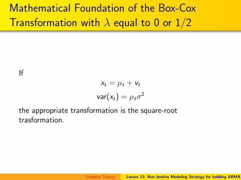
Ifxt = µt + vt

var(xt) = µ2tσ2

the appropriate transformation is the log-trasformation.




Ifxt = µt + vt

var(xt) = µtσ2

the appropriate transformation is the square-roottrasformation.




If the variance of the series appears to increasequadratically with the mean, the logarithmic

transformation (λ = 0) is appropriate;

If the variance increases linearly with the mean, weshould use λ = 0.5, that is the square-root

trasformation.


Time series


Consider the log transformation

yt = log(xt) t = 1, 2, ...,T


Time series

Figure : Log of Monthly totals in thousands of international airlinepassengers from January 1949 to December 1960.

The log transformation has removed the increasing variability.


Time series

In order to remove the trend and the seasonal component, wedecide to use the differencing method.By using the filter

∆12 = 1− L12

we remove the seasonal component

Figure : (1− L12) Log of Monthly totals in thousands of

international airline passengers


Time series

Finally, we use the filter

∆ = 1− L

in order to remove the non-stationarity in mean.


Time series

The transformed series is given by

zt = ∆∆12log(xt) t = 1, 2, ...,T

We see that the differencing has well removed the trend andthe seasonal component.

Figure : (1− L)(1− L12) Log of Monthly totals in thousands of



Time series

Figure : (1− L)(1− L12) Log of Monthly totals in thousands of


Figure : Time plot of a series generated by a stationary ARMAprocess. Umberto Triacca Lesson 13: Box-Jenkins Modeling Strategy for building ARMA

The DGP’s model

✫✪✬✩DGP

❄

ARMA

✓✓✓✓✓✓✓✓✓✓✓✼

✛✚

✘✙zk , ..., zT

✛✚

✘✙x1, ..., xT✲✛


Conclusion

After the data have been rendered stationary, we are ready tofit an appropriate model to the data. This is the subject of thenext lessons.


Lesson 13 BIS: The Identification of

ARMA Models

Umberto Triacca

Dipartimento di Ingegneria e Scienze dell’Informazione e Matematica

Universita dell’Aquila,

[email protected]

Umberto Triacca Lesson 13 BIS: The Identification of ARMA Models

Identification

Consider an ARMA process

xt ∼ ARMA(p, q)

Before an ARMA(p,q) model can be estimated we need toselect the order p and q of the AR and MA-polynomial

Following the Box and Jenkins’s terminology we will refer tothis step as identification of the appropriate ARMA model


Identification

The guidelines for the choice of p and q come from the shapeof two sample functions:

1 The Sample AutoCorrelation Function (SACF)

2 The Sample Partial AutoCorrelation Function (SPACF)


Identification

The sample autocorrelation and partial autocorrelationfunctions should reflect (with sampling variation) theproperties of the theoretical autocorrelation and partialautocorrelation functions of the process.

In order to identify the order of the model, the SACF andSPACF are compared with the theoretical ACF and PACF,respectively.

The sample autocorrelation plot and the sample partialautocorrelation plot are compared to the theoretical behaviorof these plots.


Identification

The theoretical behavior of ACF and PACF

If xt ∼ WN(0, σ2), then ρk = 0 and πk = 0 for all k ;

If xt ∼ AR(p) process, then ρk 6= 0 for all k , ρk → 0 ask → ∞ and πk 6= 0 for k ≤ p, πk = 0 for k > p;

If xt ∼ MA(q) process, then ρk 6= 0 for k ≤ q, ρk = 0 fork > q and πk 6= 0 for all k , πk → 0 as k → ∞;

If xt ∼ ARMA(p, q), then ρk 6= 0 for all k , ρk → 0 ask → ∞ and πk 6= 0 for all k , πk → 0 as k → ∞.


Identification

If xt ∼ AR(p) process, then ρk decays exponentially (eitherdirect or oscillatory) and πk cut off after the lag p.

Figure :


Identification

If xt ∼ MA(q) process, then ρk cut off after the lag q and πk

decays exponentially (either direct or oscillatory)

Figure :


Identification

If xt ∼ ARMA(p, q), then ρk decay exponentially (either director oscillatory) and πk decay exponentially (either direct oroscillatory)


Identification

The identification of a pure autoregressive or moving averageprocess is reasonably straightforward using the sampleautocorrelation and partial autocorrelation functions.

On the other hand, as we will see, for ARMA(p, q) processeswith p and q both non-zero, the SACF and SPACF are muchmore difficult to interpret


Identifying the orders p and q by using Information

Criteria

The mixed models can be particularly difficult to identify byusing the correlogram and the partial correlogram.

For this reason, in recent years information-based criteria suchas AIC (Akaike Information Criterion) and BIC (BayesInformation Criteria) and others have been preferred and used.


Model Idendification

The AIC statistic is defined as

AIC (p, q) = ln(σ2) +2(p + q)

T

where σ2 is the maximum likelihood estimated of the whitenoise variance.

Among a set of models, we select the values of p and q for ourfitted model to be those which minimize AIC (p, q).



Intuitively one can think of

2(p + q)

T

as a penality term to discourage over-parameterization.



There is an empirical evidences that AIC has the tendency topick models which are over-parameterized.

The BIC is a criterion which attempts to correct theoverfitting nature of the AIC.

It is defined to be

BIC (p, q) = ln(σ2) +ln(T )(p + q)

T



We note that BIC penalizes larger models more than AIC.

ln(T )

T>

2

T∀T ≥ 8



The procedure to use these criteria is the following:

1 Set upper bounds, P and Q for the AR and MA order,respectively

2 Fit all possible ARMA(p, q) models for p ≤ P and q ≤ Q

using a common sample size T

3 The AIC(pA, qA) and BIC(pB , qB) of the best modelssatisfy, rispectively,

AIC (pA, qA) = minp≤P,q≤QAIC (p, q)

BIC (pB , qB) = minp≤P,q≤QBIC (p, q)



The theoretical properties of these criteria have beeninvestigated. It is known that BIC is consistent in the sensethat the probability of selecting the true model approaches 1(if the true model is in the candidate list), but AIC is not.


Some examples


Some examples

The blue dotted parallel lines show approximative 95%confidence intervals for the null hypotesis H0 : ρk = 0 andH0 : πk = 0, respectively


Some examples


Some examples

Table : Selection ARMA order by AIC and BIC.

Orders p,q of ARMA model2,2 2,1 1,2 2,0 0,2 1,1

1,0 0,1

AIC 288.7 286.8 286.7 306.6 293.7 285.2

325.5 320.4BIC 304.4 299.9 299.8 317.1 304.2 289.4

333.4 328.3


lesson 13: box-jenkins modeling strategy for building arma ... · introduction in this lesson we...

Documents