lek-heng lim - cornell university · lek-heng lim university of california, berkeley february 20,...

Modeling and learning with tensors

Lek-Heng Lim

University of California, Berkeley

February 20, 2009

(Thanks: Charlie Van Loan, National Science Foundation; Collaborators: Jason Morton,

Berkant Savas, Yuan Yao)

L.-H. Lim (NSF Workshop) Tensor modeling February 20, 2009 1 / 26

Why tensors?

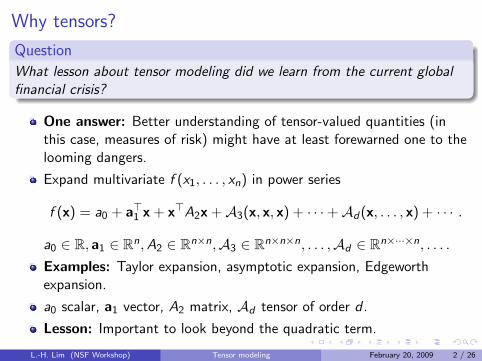
Question

What lesson about tensor modeling did we learn from the current globalfinancial crisis?

One answer: Better understanding of tensor-valued quantities (inthis case, measures of risk) might have at least forewarned one to thelooming dangers.

Expand multivariate f (x1, . . . , xn) in power series

f (x) = a0 + a>1 x + x>A2x +A3(x, x, x) + · · ·+Ad(x, . . . , x) + · · · .

a0 ∈ R, a1 ∈ Rn,A2 ∈ Rn×n,A3 ∈ Rn×n×n, . . . ,Ad ∈ Rn×···×n, . . . .

Examples: Taylor expansion, asymptotic expansion, Edgeworthexpansion.

a0 scalar, a1 vector, A2 matrix, Ad tensor of order d .

Lesson: Important to look beyond the quadratic term.


This copy is for your personal, noncommercial use only. You can order presentation-ready

copies for distribution to your colleagues, clients or customers here or use the "Reprints" tool

that appears next to any article. Visit www.nytreprints.com for samples and additional

information. Order a reprint of this article now.

January 4, 2009

Risk Mismanagement

By JOE NOCERA

‘The story that I have to tell is marked all the way through by a persistent tension between those who assertthat the best decisions are based on quantification and numbers, determined by the patterns of the past,and those who base their decisions on more subjective degrees of belief about the uncertain future. This is acontroversy that has never been resolved.’

— FROM THE INTRODUCTION TO ‘‘AGAINST THE GODS: THE REMARKABLE STORY OF RISK,’’ BYPETER L. BERNSTEIN

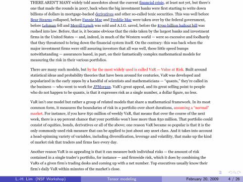
THERE AREN’T MANY widely told anecdotes about the current financial crisis, at least not yet, but there’sone that made the rounds in 2007, back when the big investment banks were first starting to write downbillions of dollars in mortgage-backed derivatives and other so-called toxic securities. This was well beforeBear Stearns collapsed, before Fannie Mae and Freddie Mac were taken over by the federal government,before Lehman fell and Merrill Lynch was sold and A.I.G. saved, before the $700 billion bailout bill wasrushed into law. Before, that is, it became obvious that the risks taken by the largest banks and investmentfirms in the United States — and, indeed, in much of the Western world — were so excessive and foolhardythat they threatened to bring down the financial system itself. On the contrary: this was back when themajor investment firms were still assuring investors that all was well, these little speed bumpsnotwithstanding — assurances based, in part, on their fantastically complex mathematical models formeasuring the risk in their various portfolios.

There are many such models, but by far the most widely used is called VaR — Value at Risk. Built aroundstatistical ideas and probability theories that have been around for centuries, VaR was developed andpopularized in the early 1990s by a handful of scientists and mathematicians — “quants,” they’re called inthe business — who went to work for JPMorgan. VaR’s great appeal, and its great selling point to peoplewho do not happen to be quants, is that it expresses risk as a single number, a dollar figure, no less.

VaR isn’t one model but rather a group of related models that share a mathematical framework. In its mostcommon form, it measures the boundaries of risk in a portfolio over short durations, assuming a “normal”market. For instance, if you have $50 million of weekly VaR, that means that over the course of the nextweek, there is a 99 percent chance that your portfolio won’t lose more than $50 million. That portfolio couldconsist of equities, bonds, derivatives or all of the above; one reason VaR became so popular is that it is theonly commonly used risk measure that can be applied to just about any asset class. And it takes into accounta head-spinning variety of variables, including diversification, leverage and volatility, that make up the kindof market risk that traders and firms face every day.

Another reason VaR is so appealing is that it can measure both individual risks — the amount of riskcontained in a single trader’s portfolio, for instance — and firmwide risk, which it does by combining theVaRs of a given firm’s trading desks and coming up with a net number. Top executives usually know theirfirm’s daily VaR within minutes of the market’s close.


properly understood, were not a fraud after all but a potentially important signal that trouble was brewing?Or did it suggest instead that a handful of human beings at Goldman Sachs acted wisely by putting theirmodels aside and making “decisions on more subjective degrees of belief about an uncertain future,” asPeter L. Bernstein put it in “Against the Gods?”

To put it in blunter terms, could VaR and the other risk models Wall Street relies on have helped preventthe financial crisis if only Wall Street paid better attention to them? Or did Wall Street’s reliance on themhelp lead us into the abyss?

One Saturday a few months ago, Taleb, a trim, impeccably dressed, middle-aged man — inexplicably, hewon’t give his age — walked into a lobby in the Columbia Business School and headed for a classroom togive a guest lecture. Until that moment, the lobby was filled with students chatting and eating a quick lunchbefore the afternoon session began, but as soon as they saw Taleb, they streamed toward him, surroundinghim and moving with him as he slowly inched his way up the stairs toward an already-crowded classroom.Those who couldn’t get in had to make do with the next classroom over, which had been set up as anoverflow room. It was jammed, too.

It’s not every day that an options trader becomes famous by writing a book, but that’s what Taleb did, firstwith “Fooled by Randomness,” which was published in 2001 and became an immediate cult classic on WallStreet, and more recently with “The Black Swan: The Impact of the Highly Improbable,” which came out in2007 and landed on a number of best-seller lists. He also went from being primarily an options trader towhat he always really wanted to be: a public intellectual. When I made the mistake of asking him one daywhether he was an adjunct professor, he quickly corrected me. “I’m the Distinguished Professor of RiskEngineering at N.Y.U.,” he responded. “It’s the highest title they give in that department.” Humility is notamong his virtues. On his Web site he has a link that reads, “Quotes from ‘The Black Swan’ that theimbeciles did not want to hear.”

“How many of you took statistics at Columbia?” he asked as he began his lecture. Most of the hands in theroom shot up. “You wasted your money,” he sniffed. Behind him was a slide of Mickey Mouse that he hadput up on the screen, he said, because it represented “Mickey Mouse probabilities.” That pretty much sumsup his view of business-school statistics and probability courses.

Taleb’s ideas can be difficult to follow, in part because he uses the language of academic statisticians; wordslike “Gaussian,” “kurtosis” and “variance” roll off his tongue. But it’s also because he speaks in a kind ofbrusque shorthand, acting as if any fool should be able to follow his train of thought, which he can’t bebothered to fully explain.

“This is a Stan O’Neal trade,” he said, referring to the former chief executive of Merrill Lynch. He clicked toa slide that showed a trade that made slow, steady profits — and then quickly spiraled downward for a giant,brutal loss.

“Why do people measure risks against events that took place in 1987?” he asked, referring to Black Monday,the October day when the U.S. market lost more than 20 percent of its value and has been used ever since asthe worst-case scenario in many risk models. “Why is that a benchmark? I call it future-blindness.

“If you have a pilot flying a plane who doesn’t understand there can be storms, what is going to happen?” heasked. “He is not going to have a magnificent flight. Any small error is going to crash a plane. This is whythe crisis that happened was predictable.”

Eventually, though, you do start to get the point. Taleb says that Wall Street risk models, no matter how


Cumulants

Univariate distribution: First four cumulants areI mean K1(x) = E(x) = µ,I variance K2(x) = Var(x) = σ2,I skewness K3(x) = σ3 Skew(x),I kurtosis K4(x) = σ4 Kurt(x).

Multivariate distribution: Covariance matrix partly describes thedependence structure — enough for Gaussian. Cumulants describehigher order dependence among random variables.


Cumulants

For multivariate x, Kd(x) = Jκj1···jd (x)K are symmetric tensors oforder d .

In terms of Edgeworth expansion,

log E(exp(i〈t, x〉) =∞∑

α=0

i |α|κα(x)tα

α!, log E(exp(〈t, x〉) =

∞∑α=0

κα(x)tα

α!,

α = (j1, . . . , jn) is a multi-index, tα = t j11 · · · t

jnn , α! = j1! · · · jn!.

Provide a natural measure of non-Gaussianity: If x Gaussian,

Kd(x) = 0 for all d ≥ 3.

Gaussian assumption equivalent to quadratic approximation.

Non-Gaussian data: Not enough to look at just mean andcovariance.


Tensors inevitable in multivariate problems

Mathematics

I Derivatives of univariate functions: f : R→ R smooth,f ′(x), f ′′(x), . . . , f (k)(x) ∈ R.

I Derivatives of multivariate functions: f : Rn → R smooth,grad f (x) ∈ Rn,Hess f (x) ∈ Rn×n, . . . ,D(k)f (x) ∈ Rn×···×n.

Statistics

I Cumulants of random variables: Kd(x) ∈ R.I Cumulants of random vectors: Kd(x) = Jκj1···jd (x)K ∈ Rn×···×n.

Physics

I Hooke’s law in 1D: x extension, F force, k spring constant,

F = −kx .

I Hooke’s law in 3D: x = (x1, x2, x3)>, elasticity tensor C ∈ R3×3×3×3,stress Σ ∈ R3×3, strain Γ ∈ R3×3

σij =∑3

k,l=1cijklγkl .


Humans cannot understand tensorsHumans cannot make sense out of more than O(n) numbers. For mostpeople, 5 ≤ n ≤ 9 [Miller, 1956].

VaR: single numberI Readily understandable.I Not sufficiently informative and discriminative.

Covariance matrix: O(n2) numbersI Hard to make sense of without further processing.I For symmetric matrices, may perform eigenvalue decomposition.I Basis for PCA, MDS, ISOMAP, LLE, Laplacian Eigenmap, etc.I Used in clustering, classification, dimension reduction, feature

identification, learning, prediction, visualization, etc.

Cumulant of order d : O(nd) numbersI How to make sense of these?I Want analogue of ‘eigenvalue decomposition’ for symmetric tensors.I Principal Cumulant Component Analysis: finding components that

simultaneously account for variation in cumulants of all orders (cf.Jason Morton’s talk).


DARPA mathematical challenge eight

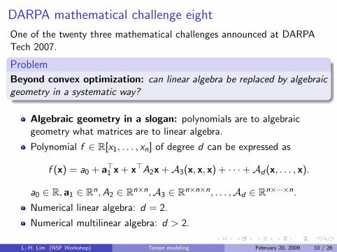
One of the twenty three mathematical challenges announced at DARPATech 2007.

Problem

Beyond convex optimization: can linear algebra be replaced by algebraicgeometry in a systematic way?

Algebraic geometry in a slogan: polynomials are to algebraicgeometry what matrices are to linear algebra.

Polynomial f ∈ R[x1, . . . , xn] of degree d can be expressed as

f (x) = a0 + a>1 x + x>A2x +A3(x, x, x) + · · ·+Ad(x, . . . , x).

a0 ∈ R, a1 ∈ Rn,A2 ∈ Rn×n,A3 ∈ Rn×n×n, . . . ,Ad ∈ Rn×···×n.

Numerical linear algebra: d = 2.

Numerical multilinear algebra: d > 2.


Tensors as hypermatrices

Up to choice of bases on U,V ,W , a tensor A ∈ U ⊗ V ⊗W may berepresented as a hypermatrix

A = JaijkKl ,m,ni ,j ,k=1 ∈ Rl×m×n

where dim(U) = l , dim(V ) = m, dim(W ) = n if

1 we give it coordinates;

2 we ignore covariance and contravariance.

Henceforth, tensor = hypermatrix.


Probably the source

Woldemar Voigt, Die fundamentalen physikalischen Eigenschaften derKrystalle in elementarer Darstellung, Verlag Von Veit, Leipzig, 1898.

“An abstract entity represented by an array of componentsthat are functions of co-ordinates such that, under atransformation of co-ordinates, the new components are relatedto the transformation and to the original components in adefinite way.”


Definite way: multilinear matrix multiplication

Correspond to change-of-bases transformations for tensors.

Matrices can be multiplied on left and right: A ∈ Rm×n, X ∈ Rp×m,Y ∈ Rq×n,

C = (X ,Y ) · A = XAY> ∈ Rp×q,

cαβ =∑m,n

i ,j=1xαiyβjaij .

3-tensors can be multiplied on three sides: A ∈ Rl×m×n, X ∈ Rp×l ,Y ∈ Rq×m, Z ∈ Rr×n,

C = (X ,Y ,Z ) · A ∈ Rp×q×r ,

cαβγ =∑l ,m,n

i ,j ,k=1xαiyβjzγkaijk .

Define ‘right’ (covariant) multiplication by(X ,Y ,Z ) · A = A · (X>,Y>,Z>).


Not every 3-array of numbers is a 3-tensor

3-way array: data structure; 3-tensor: algebraic object.

Saying that a measured or observed 3-array of numbers is a 3-tensoris a modeling process.

Should have some reason to believe that these numbers transform asexpected under change-of-bases, i.e. via multilinear matrixmultiplications.

Not a 3-tensor:

I Take n × 3n matrix representing a linear operator from an3n-dimensional vector space to an n-dimensional vector space and writeit as n × n × n array of numbers.

I iPod sales figures stored in a ZIP code-by-model number-by-montharray.

I Phone directory — page-by-row-by-column of phone numbers.


Tensor modeling in physics

Hooke’s law revisited: At a point x = (x1, x2, x3)> in a linearanisotropic solid,

σij =∑3

k,l=1cijklγkl −

∑3

k=1bijkek − taij

where elasticity tensor C ∈ R3×3×3×3, piezoelectric tensorB ∈ R3×3×3, thermal tensor A ∈ R3×3, stress Σ ∈ R3×3, strainΓ ∈ R3×3, electric field e ∈ R3, temperature change t ∈ R.

Invariant under change-of-coordinates: If y = Qx, then

σij =∑3

k,l=1c ijklγkl −

∑3

k=1bijkek − taij

where

C = (Q,Q,Q,Q) · C, B = (Q,Q,Q) · B, A = (Q,Q) · A,Σ = (Q,Q) · Σ, Γ = (Q,Q) · Γ, e = Qe.


Tensor modeling in statistics

Multilinearity: If x is a Rn-valued random variable and A ∈ Rm×n

Kp(Ax) = (A, . . . ,A) · Kp(x).

Additivity: If x1, . . . , xk are mutually independent of y1, . . . , yk , then

Kp(x1 + y1, . . . , xk + yk) = Kp(x1, . . . , xk) +Kp(y1, . . . , yk).

Independence: If I and J partition {j1, . . . , jp} so that xI and xJ areindependent, then

κj1···jp (x) = 0.

Support: There are no distributions where

Kp(x)

{6= 0 3 ≤ p ≤ n,

= 0 p > n.


Tensor modeling in computer science

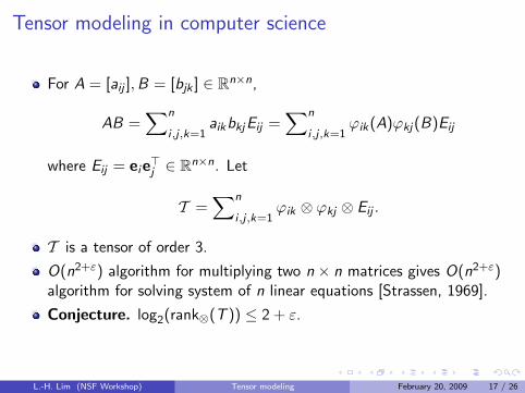
For A = [aij ],B = [bjk ] ∈ Rn×n,

AB =∑n

i ,j ,k=1aikbkjEij =

∑n

i ,j ,k=1ϕik(A)ϕkj(B)Eij

where Eij = eie>j ∈ Rn×n. Let

T =∑n

i ,j ,k=1ϕik ⊗ ϕkj ⊗ Eij .

T is a tensor of order 3.

O(n2+ε) algorithm for multiplying two n × n matrices gives O(n2+ε)algorithm for solving system of n linear equations [Strassen, 1969].

Conjecture. log2(rank⊗(T )) ≤ 2 + ε.


How do tensors arise in modeling?

Affinity or dissimilarity of triples of objects: symmetric tensors.I Example: Amit Singer’s dissimilarity metric from cryo-EM and NMR

applications. A = JaijkK ∈ S3(Rn) where

aijk = exp

[−

d2ij + d2

jk + d2ki

δ

]× exp

[−1

εsin2

(θij + θjk + θki

2

)].

May assume, for simplicity, aijk = wijwjkwki for some nonnegativematrix W = [wij ] ∈ S2(Rn).

Measure of higher order dependence: symmetric tensors.I Example: Cumulants.

Comparisons of triples of objects: skew-symmetric tensors.I Example: Triplewise rankings.

Multilinearity: tensors.I Example: If all but one factors are kept constant and the quantity you

are measuring varies linearly with the changing factor, then thatquantity can be modeled by a tensor.


Analyzing tensorsA ∈ Rm×n.

I Singular value decomposition:

A = UΣV> =∑r

i=1σiui ⊗ vi

where rank(A) = r , U,V orthonormal columns, Σ = diag[σ1, . . . , σr ].

A ∈ Rl×m×n. Can either keep diagonality of Σ or orthogonality of Uand V but not both.

I Linear combination:

A = (X ,Y ,Z ) · Σ =∑r

i=1σixi ⊗ yi ⊗ zi

where rank⊗(A) = r , X ,Y ,Z matrices, Σ = diagr×r×r [σ1, . . . , σr ]; rmay exceed n.

I Multilinear combination:

A = (U,V ,W ) · C =∑r1,r2,r3

i,j,k=1cijkui ⊗ vj ⊗wk

where rank�(A) = (r1, r2, r3), U,V ,W orthonormal columns,C = JcijkK ∈ Rr1×r2×r3 ; r1, r2, r3 ≤ n.

I Ensuing models in Psychometrics: candecomp/parafac and Tucker.


Other forms

Approximation theory: Decomposing function into linearcombination of separable functions,

f (x , y , z) =∑r

i=1λiϕi (x)ψi (y)θi (z).

Application: separation of variables for pdes.

Operator theory: Decomposing operator into linear combination ofKronecker products,

∆3 = ∆1 ⊗ I ⊗ I + I ⊗∆1 ⊗ I + I ⊗ I ⊗∆1.

Application: numerical operator calculus (cf. talks by Greg Beylkin,Martin Mohlenkamp).


Other forms

Commutative algebra: Decomposing homogeneous polynomial intolinear combination of powers of linear forms,

pd(x , y , z) =∑r

i=1λi (aix + biy + ciz)d .

Application: independent components analysis (cf. talks by PhilipRegalia, Lieven De Lathauwer).

Probability theory: Decomposing probability density into conditionaldensities of random variables satisfying naıve Bayes:

Pr(x , y , z) =∑

hPr(h) Pr(x | h) Pr(y | h) Pr(z | h).

Application: probabilistic latent semantic indexing (cf. talks byInderjit Dhillon, Haesun Park, Bob Plemmons).

H◦

X•oo

oooo

Y•

Z•O

OOOOO


Multilinear spectral theory

Eigenvalues and eigenvectors of symmetric A ∈ Rn×n are criticalvalues and critical points of

x>Ax/‖x‖22.

Define eigenvalues/vectors of symmetric tensor A as criticalvalues/points of

A(x, . . . , x)/‖x‖pp.I Liqun Qi independently defined essentially the same notion in a

different manner.I Falls outside Classical Invariant Theory — not invariant under

Q ∈ O(n), ie. ‖Qx‖2 = ‖x‖2.

Define singular values/vectors of tensor A as critical values/points of

A(u, v . . . , z)

‖u‖2‖v‖2 · · · ‖z‖2.

I σmax(A) equals spectral norm of A.


Inherent difficulty

The best r -term approximation problem for tensors has no solution ingeneral (except for the nonnegative case).

Eugene Lawler: “The Mystical Power of Twoness.”

I 2-SAT is easy, 3-SAT is hard;I 2-dimensional matching is easy, 3-dimensional matching is hard;I 2-body problem is easy, 3-body problem is hard;I 2-dimensional Ising model is easy, 3-dimensional Ising model is hard.

Applies to tensors too:

I 2-tensor rank is easy, 3-tensor rank is hard;I 2-tensor spectral norm is easy, 3-tensor spectral norm is hard;I 2-tensor approximation is easy, 3-tensor approximation is hard;I 2-tensor eigenvalue problem is easy, 3-tensor eigenvalue problem is

hard.


Functions and operators on graphG = (V ,E ) undirected graph.

FunctionsI vertices: s : V → R, s(i) = si ;I edges: X : V × V → R, X (i , j) = Xij = 0 if {i , j} 6∈ E ,

Xij = −Xji ;

I triangles: Φ : V × V × V → R, Φ(i , j , k) = Φijk = 0 if {i , j , k} 6∈ T ,

Φijk = Φjki = Φkij = −Φjik = −Φikj = −Φkji .

OperatorsI grad : L2(V )→ L2(E ), grad s(i , j) = sj − si ;I curl : L2(E )→ L2(T ), curl X (i , j , k) = Xij + Xjk + Xki ;I div : L2(E )→ L2(V ), div X (i) =

∑j wijXij ;

I graph Laplacian: ∆0 : L2(V )→ L2(V ),

∆0 = div ◦ grad;

I graph Helmholtzian: ∆1 : L2(E )→ L2(E ),

∆1 = curl∗ ◦ curl− grad ◦ div .


Ranking with tensors

Theorem (Helmholtz decomposition)

Let G = (V ,E ) be an undirected, unweighted graph and ∆1 itsHelmholtzian. The space of edge flows on G admits an orthogonaldecomposition

L2(E ) = im(grad)⊕ ker(∆1)⊕ im(curl∗).

Furthermore, ker(∆1) = ker(curl) ∩ ker(div).

For each triangle {i , j , k}, curl(X )(i , j , k) measures inconsistencyalong the loop i → j → k → i .Bottomline: resolve aggregated pairwise rankings X ∈ L2(E ) into

X = grad s + H + curl∗Φ.

I s gives us a global ranking of the alternatives;I the residual X − grad s is a certificate of reliability for s;I sizes of H and curl∗Φ tell us whether the inconsistencies are of a global

or local nature.

Joint work with Yuan Yao.L.-H. Lim (NSF Workshop) Tensor modeling February 20, 2009 25 / 26

Kernel learning with tensors?

Given training data (xi , yi ), i = 1, . . . , n, want to ‘learn’ targetfunctions

I f : {e-mails} → {−1, 1}, f (x) = −1 if x is spam, f (x) = 1 otherwise;I g : {SNPs} → [−1, 1], g(x) = likelihood that x plays a role in diabetes;I h : {hand-written digits} → {0, 1, 2, . . . , 9}.

Take Galerkin approach:I assume

f (x) =∑n

i=1αiK (x , xi ),

K Mercer kernel, e.g. K (x , y) = exp(−‖x − y‖2/σ2);I solve regularized least-squares for α1, . . . , αn,

min∑n

i=1[y − f (xi )]2 + λ‖f ‖2.

Work in progress (with Jason Morton): extend this to symmetricnuclear forms

K (x , y , z) =∑∞

k=1λkϕk(x)ϕk(y)ϕk(z).


lek-heng lim - cornell university · lek-heng lim university of california, berkeley february 20,...

Documents