FRIEDRICH-ALEXANDER-UNIVERSITAT ERLANGEN-NURNBERGINSTITUT FUR INFORMATIK (MATHEMATISCHE MASCHINEN UND DATENVERARBEITUNG)

Lehrstuhl fur Informatik 10 (Systemsimulation)

waLBerla: Visualization of Fluid Simulation Data with POV-Ray

Simon Bogner, Stefan Donath, Christian Feichtinger, Ulrich Rude

Technical Report 09-13

waLBerla: Visualization of Fluid SimulationData with POV-Ray

Simon Bogner, Stefan Donath, Christian Feichtinger, Ulrich Rude

Lehrstuhl fur SystemsimulationFriedrich-Alexander University of Erlangen-Nuremberg

91058 Erlangen, Germany

walberla@i10.informatik.uni-erlangen.de

December 14, 2009

Contents

1 Introduction 3

2 Feature Outline 4

3 File Structure and Output Directory Structure 53.1 Scene Composition . . . . . . . . . . . . . . . . . . . . . . . . . . . . . . . . . . . . . . . . 63.2 Resources and Visualization Types . . . . . . . . . . . . . . . . . . . . . . . . . . . . . . . 6

4 pe Objects 9

5 DensFields 105.1 File Structure . . . . . . . . . . . . . . . . . . . . . . . . . . . . . . . . . . . . . . . . . . . 105.2 Usage . . . . . . . . . . . . . . . . . . . . . . . . . . . . . . . . . . . . . . . . . . . . . . . 10

6 CellFields 176.1 Usage and Output File Structure . . . . . . . . . . . . . . . . . . . . . . . . . . . . . . . . 176.2 Porous Medium Example . . . . . . . . . . . . . . . . . . . . . . . . . . . . . . . . . . . . 17

7 Free Surface Visualization 207.1 Free Surface Extraction . . . . . . . . . . . . . . . . . . . . . . . . . . . . . . . . . . . . . 207.2 Usage and Examples . . . . . . . . . . . . . . . . . . . . . . . . . . . . . . . . . . . . . . . 20

8 Conclusion 23

1 Introduction

The waLBerla framework is a versatile, parallel fluid solver based on the lattice Boltzmann method(LBM). The acronym waLBerla stands for w idely applicable lattice Boltzmann solver from Erlangen.Besides simulation of simple fluid flow, it supports a variety of different applications involving multi-phaseand free surface flows and particulate flows with fully resolved, moving particles [DGF+07, GFI+08]. Toenable efficient analysis of the simulation outcome, waLBerla features different means of data visualization.Parallel generic modules [GDF+07b] enable plotting of computed values into XMGrace-compatible graphsand writing of arbitrary, cell-based data to file formats of the visualization tool kit (VTK) [VTK09] thatcan be viewed and further analyzed by VTK-based tools like ParaView [Par09]. Besides value-basedvalidation, a realistic visualization of the flow and its characteristic quantities is important and of availbecause human intuition is best proof for nature’s behavior. Consequently, waLBerla has been extentedby a generic module for output files that are readable by POV-Ray, which is a well-known ray tracertool [oVPL04]. Thus, the motion would become visible by rendering images of different time steps withthe POV-Ray raytracer. Initially developed to only visualize particulate flows, this waLBerla module hasbeen enhanced in order to be compatible with free surface flows, too, and be able to visualize scientificrelevant data like densities, velocities and forces. This report gives a detailed insight into the technicalrealization of a flexible interface between waLBerla and POV-Ray, using the POV-Ray scene descriptionlanguage (SDL).

3

2 Feature Outline

WaLBerla can create special output data using the POV-Ray scene description language (SDL). SDL isa language used to define a 3-dimensional world consisting of various geometrical shapes, light sources,etc... The following list gives a rough summary of the output options currently provided by waLBerla.

DensField: A DensField is a 3-dimensional array of floating point values. As described in [GDF+07a],waLBerla holds the simulation data in Fields. WaLBerla can be instructed to write out the valuesof any field of type ScalarField<Real> or type VecField<Real> (DensField1 and VelField, inwhich waLBerla stores the macroscopic values of density and fluid velocity, are also possible) in anaxis-aligned subregion as a DensField. Typical application: Visualization of the velocity or densityprofile of a flow.

CellField: CellFields can be used to visualize the waLBerla FlagField. A CellField is thus an axis-alignedsubregion of the FlagField. Usually one is interested in cells of a certain flag state only. Typicalapplication: Visualization of the geometry of a porous medium.

FreeSurface: If a free surface flow is simulated, the behavior of the free surface may be visualized eitherby its surface normals, which can be shown as glyphs, or by a triangle mesh resembling the freesurface. Typical application: Visualization of two-phase free surface flows, such as foams.

Obstacles: The various kinds of obstacles (i.e. particles, walls, etc.) supported by waLBerla (see[GDF+07b]) can be visualized. Typical application: Visualization of particle suspensions.

Ray tracing is a powerful way to create images from spatial information, but because of its computation-intensive nature it is far from being interactive. In spite of this limitation, one of the main design goalswas to provide the user with as much flexibility as possible, i.e., to provide the output not only in a formatadapted to POV-Ray, but also well-readable and modifiable for the user. The SDL files generated bywaLBerla can be edited to adjust the output files to change the properties (point of view, light sources,colors and textures of objects, etc.) of the final images. The following section treats the activation ofPOV-Ray output via waLBerla parameter files. An overview of the most important output files and filedependencies is given. Also the incorporation of external resources, e.g. textures, to a visualization isexplained. For the actual usage and visualization options of DensFields, CellFields, FreeSurfaces andObstacles, respectively, own sections have been devoted. It is suggested to the reader to take a look onthe next section carefully and then continue with a section of his interest.

1Name coincidence: There is also a waLBerla-internal scalar field called DensField!

4

3 File Structure and Output Directory Structure

In order to facilitate POV-Ray visualizations, the various output options have been integrated in thewaLBerla parameter file. A povray block has to be specified by the user in order to activate and controlthe POV-Ray specific output. Listing 1 exemplarily shows a typical povray block that would createan output directory named /simdata/povray. In the output directory waLBerla creates the directorystructure shown in Fig. 3.

Figure 1: Directory Structure

./dat contains the data to be rendered

/0 objects/data written by process 1.

/1 objects/data written by process 2.

...

./plane velocity planes (not subject of this report)

/0 objects/data written by process 1.

/1 objects/data written by process 2.

...

./png empty output directory for final images rendered by POV-Ray

./res include files for POV-Ray

/resource1.inc user-declared include file 1

/resource2.inc user-declared include file 2

...

./Globals.inc global declarations and scene composition for the POV-Ray visualization

./Cam0.pov Camera 0

./Cam1.pov Camera 1

...

./GenerateMPG.py a python script that calls FFmpeg to create animations from rendered images.

./GeneratePOV.py a python script that calls POV-Ray to render the final images.

Inside the povray block, the spacing keyword specifies how often data is written to the ./dat direc-tory in the output directory specified by filename. Since a simulation may run on multiple processesin parallel, each process will store its data in a subdirectory named by the process number. All objects(DensFields, obstacles, etc.) for the visualization are stored in these subdirectories, depending on whichprocess the respective data is computed. For more details on waLBerla parallelization, please refer to[GDF+07b]. The data output files of different time steps for each object are numbered in subsequentorder starting from zero - irrespective of the setting of the spacing variable. To eventually compose thewritten objects to a scene, waLBerla creates the file ./Globals.inc, which will be described in the nextsubsection.Inside the povray block, one ore more cameras have to be defined in the form of camera blocks. For eachcamera, individual light sources can be added to the scene. Each camera block leads to the creation ofa file ./Cam<number>.pov, where number is substituted by the number of the camera. The camera fileautomatically includes the scene file ./Globals.inc. For more information on cameras and light sourcesplease refer to the POV-Ray documentation [oVPL04].Additionally the user can instruct the inclusion of external POV-Ray resources to the file ./Globals.inc

5

Listing 1: Povray block examplepovray {

spac ing 10 ; // wr i te data every 10 . th time stepf i l ename / simdata/povray ; // d i r e c t o r y to c r ea t e f i l e −s t ru c tu r e in

camera {po s i t i on L <−25,−25,75>; // po s i t i on o f the cameralookAt L <25 ,25 ,25>; // c on t r o l s the look−d i r e c t i o n o f the camera

po i n t l i g h t { // automat i ca l ly add a l i g h t source f o r t h i s camerapo s i t i on L <−25, −25, 75>; // l i g h t po s i t i onrgb <1 ,1 ,1>; // l i g h t c o l o r

}

a r e a l i g h t { // another type o f l i g h t sourcepo s i t i on L <10, 1 , 40>;l ow e r l e f t L <15, 0 , 0>;t op r i gh t L <0, 0 , 15>;sample x 1 ;sample y 1 ;f ad e d i s t an c e 120 ;fade power 1 ;

}}

// ’ resource ’ b locks can be used to inc lude add i t i ona l sd l f i l e s in povrayre source {

f i l e ” t ex tu r e s . inc ” ; // povray standard t ex tu r e s}r e source { f i l e examples /povray/ r e s ou r c e s /Textures . dat ; } // user de f ined t ex tu r e s

}

by specifying an arbitrary number of resource blocks. Each resource block must have one file pa-rameter defined, which is either the file name of a user-created file or a standard include file provided byPOV-Ray. In the latter case, the file name must be given in the form ’’<filename>’’. In the former case,the external file will automatically be copied into the output directory as ./res/resource<number>.inc.Again, the files are tagged with a number <number>. This is useful in order to add external resources(textures, color maps, etc.) to the scene. See also Sec. 3.2.

3.1 Scene Composition

Figure 2 exemplarily shows the dependencies of files for a project with two parallel processes and threecameras defined. As described above there will typically be multiple files for each object. Each waLBerlaprocess creates one output file per written time step for every object residing on the respective process.These files are composed to a scene in the file ./Globals.inc. Since single objects may reside on differentwaLBerla processes, and therefore the output data may reside in different directories, multiple files mayhave to be included for one and the same object (see Fig. 3). Even though there may be data writtenfrom different time steps, of course only files of the same time step are used to compose the scene: Toinclude all files of a given time step, a control variable timestep is used. This variable may be set by theuser to specify the time step to be rendered. By default, the internal POV-Ray variable frame_number isused to select the time step. See the chapter on animation in the POV-Ray documentation [oVPL04] formore information on the frame_number variable.

3.2 Resources and Visualization Types

To control the looks of rendered objects, POV-Ray provides a wide range of options. According tothe POV-Ray documentation [oVPL04], textures control how the surface of an object is rendered, whileinteriors can be used to describe the properties of the interior of an object. To specify the looks of anobject over a waLBerla parameter file, waLBerla allows the definition of visualization types (PovVisTypeblock) inside the povray block. Every visualization type needs to have its own unique identificationnumber (id) defined. The id of the visualization type can then be assigned to an object, to determinehow it is rendered by POV-Ray. Concrete examples of this will be given in the subsequent sections.

Listing 2 illustrates all keywords that are allowed inside a PovVisType block. The Parameters texture,interior and macro expect identifiers of textures, interiors and macros, respectively. For example,

6

Figure 2: File dependencies of POV-Ray output

Listing 2: Sample POV-Ray Visualization Typepovray {

. . .

PovVisType{

id 1 ;t exture DMFWood6; // su r f a c e texture o f ob j e c ti n t e r i o r Minera lOi l Int ; // i n t e r i o r o f an ob j e c tmacro Den s i t y In t e r i o r ; // macro app l i ed to the ob j e c t ( advanced e f f e c t s )

hol low ; // render the i n t e r i o r o f the ob j e c tno shadow ; // ob j e c t c a s t s no shadow

// the f o l l ow ing block s p e c i f i e s photon render ing behavior o f the ob j e c t// needed only f o r ob j e c t s that cause r e f r a c t i o n e f f e c t s such as f r e e s u r f a c e sphotons{

c o l l e c t ; // photons become v i s i b l e i f they h i t the ob j e c t ( not recommended f o r r e f r a c t i n g ob j e c t s)

t a rge t ; // do photon render ing f o r t h i s ob j e c tr e f l e c t i o n ; // c a l c u l a t e r e f l e c t i o n o f photonsr e f r a c t i o n ; // c a l c u l a t e r e f r a c t i o n o f photons

}

// the f o l l ow ing keywords make sense f o r moving ob s t a c l e s onlytrack ; // track the path o f the ob j e c tf o r c e ; // v i s u a l i z e the net f o r c e on the ob j e c t

}

. . .}

7

DMFWood6 actually is a texture that is declared in the ‘‘textures.inc’’ include file which ships withPOV-ray. However, it is up to the user to provide well defined identifiers for the visualization type. Thereis no error checking done by waLBerla at this point. Thus it is possible to run the simulation in waLBerlaand provide the missing POV-Ray declaration for resources afterwards. Moreover, it is possible to directlyinsert POV-Ray expressions here, for example

t exture pigment{rgbt 0 .9 // almost t ransparent su r f a c e texture

} ;

Any expression that is allowed in a POV-Ray texture, interior or macro, respectively, is possible, aslong as it does not contain any delimitor (i.e. semicolon). The most flexible way however is to declare allresources in external files and refer to them by their identifiers in visualization type definitions as statedbefore: Thus to modify or replace the resources in the final visualization, only the respective declarationsneed to be changed. The remaining keywords in the PovVisType block and the Photons sub-block areboolean type parameters. The particular option will be turned on if the keyword is present, and turnedoff otherwise. The track and force options only apply if the visualization type is assigned to a movingobstacle (see Sec. 4). hollow and no_shadow turn on the respective POV-Ray options of the same namefor the affected objects. The same holds for the options collect, target, reflection and refractionin the photons block. Note, that the latter are ignored by POV-Ray as long as photon mapping isnot activated in POV-Ray’s global settings while ray tracing. Photon mapping is only interesting whenreflective or refractive objects are visualized, such as free surfaces (Sec. 7). For more information, readthe section on photon mapping in the POV-Ray documentation [oVPL04].

8

4 pe Objects

Moving or fixed obstacles that are handled by the pe engine are automatically included in waLBerla’s POV-Ray output. For the integration of the pe engine in waLBerla please refer to [GDF+07b]. For every writtentime step the obstacle geometry is written to the files ./dat/<pid>/Obstacles<framenumber>.dat, de-pending on the number <pid> of the process an obstacle resides on. <framenumber> indicates the numberof the time step. A standard texture is used for all pe objects, unless another visualization type is assignedto the object. This can be done by adding a povvistype statement to the defining block of the objectin the parameter file. The definition of visualization types is described in Sec. 3.2. When applied to amoving obstacle, the special feature of tracking the path of its movement may be activated by the trackkeyword in the according povvistype block. Also, the net force on an obstacle may be visualized as acone pointing away from the obstacle in the force direction. Force visualization is activated by the forcekeyword. A sample object definition is given in listing 3.

Listing 3: Sample object blockinner{

sphere {id 1 ; // User − s p e c i f i c ID of the spherepo s i t i on L <’domainX ’/2 .0 , ’ domainY ’/2 .0 , ’ domainZ ’/2 .0 >; // Global po s i t i on o f the sphererad ius L ’ domainZ ’ / 8 . 0 ; // Radius o f the spheremater ia l{

mater ia l myMaterial ;dens i ty 10 ; // dens i ty o f the sphere ’ s mater ia l

}

povvistype 1 ; // v i s u a l i z a t i o n type o f sphere}

. . .}

WaLBerla also writes the exact position of every object to the POV-Ray files. The position and rotation ofan object can be accessed by the identifier object<id>_position and object<id>_rotation, respectively,where <id> is the id of the object. Both position and rotation are float-valued vectors of length 3. Thiscan be used, for example, to make the camera focus the object like in the following:camera{

l o c a t i on <0,25,−25>;l o ok a t ob j e c t1 pos ;sky <0 ,1 ,0>;

}

See the POV-Ray documentation [oVPL04] for more information on the camera object.

9

5 DensFields

DensFields can be used to visualize waLBerla fields of type Real or more precisely any waLBerla field oftype DensField, VelField, ScalarField<Real> and VecField<Real>. The term DensField originatesfrom POV-Ray [oVPL04], where a density can be thought of as a function in 3-dimensional space thatmaps every point to a density value in between 0 and 1. This makes it possible to render every point onor inside an object differently depending on the density value at that point. A DensField is basically sucha density pattern that was created from one of waLBerla’s data fields.

5.1 File Structure

POV-Ray supports the definition of density patterns by providing a 3D bitmap read from a file. Accordingto the POV-Ray documentation [oVPL04] every voxel in the df3 file format is an unsigned integer valueof either 1, 2 or 4 bytes. These values are scaled into a float value in the range 0.0 to 1.0 by POV-Ray. If aDensField is defined in the parameter file, every process will create one df3 file for every local patch in everywritten time step, which is named ./dat/<pid>/DensField<id>Patch<patchnumber>_<framenumber>.Here <pid> is the number of the process, <id> is the number of the DensField, <patchnumber> is thenumber of the patch and <framenumber> is the number of the written time step. The id is simply aninteger number that is used by waLBerla to distinguish between various DensFields. In addition anSDL include file ./dat/<pid>/DensField<id>.inc is written for every process, which defines an accessfunction densfunction<id>process<pid>(x,y,z) to the density values stored for the local patches. Thisfunction will return 0 if the argument (x, y, z) is not within the range of the patches of the process. Ifthereby densfield<id>_interpolation is defined as a positive value, the values of every patch will beinterpolated accordingly. However, POV-Ray will not interpolate the values at the borders of patches.This is because POV-Ray’s internal interpolation routines only work per df3 file. Even though the fieldvalues in the ghost layer is written out in the case that the border of a patch lies within the range ofthe DensField, such that the df3 files “overlap”, POV-Ray’s interpolation will still lead to wrong resultsin general. This is due to the fact that there is no guarantee, that the macroscopic values in the layerhave been communicated or calculated, respectively, before the data is written. Whether communicationhas to be done between patches depends on the field type, making a generic solution rather expensive toimplement. As an alternative, one could implement in POV-Ray’s SDL an interpolation routine, whichthen interpolates the values of different df3 files where needed, instead of using the internal interpolationroutines. See the POV-Ray documentation [oVPL04] on interpolation of density patterns.

To write the waLBerla field values to the df3 files, the following conversion formula is used.

d(x, y, z) = bf(x, y, z)− fmin

fmax − fmin· 28·pc (1)

Here, f(x, y, z) is the value of the waLBerla data field at position (x, y, z). If the field to be written is notof scalar type but a vector field, then f(x, y, z) is the euclidian norm of the vector at position (x, y, z).Floating point numbers in the interval [fmin, fmax] are mapped to the interval [0..28·p] of integers, with pbeing the number of bytes of the integer. Values below fmin or above fmax will be mapped to 0 or 28·p,respectively.The above function can easily be inverted to reobtain the original field values up to roundoff errors as

f(x, y, z) =d(x, y, z)

28·p · (fmax − fmin) + fmin. (2)

The constants fmin, fmax and p have to be specified by the user, as described in the following section.

5.2 Usage

To create a DensField with waLBerla, a DensField block has to be added to the parameter file. DensFieldblocks have to be specified inside the povray block. A Densfield is always contained by an axis-aligned

10

box inside the domain. Listing 4 shows a DensField, which extracts exactly the slice of cells with z = 25of the domain. The field parameter specifies the data field to be written. A field identifier stringis expected here, e.g., FIELD_DENS or FIELD_VELOCITY . The parameter range is used to specify theconstants fmin, fmax from Eq. 1 and Eq. 2. precision controls the precision of the written values asdescribed above and must be set to either 1, 2 or 4 [bytes]. Finally, the parameter povvistype can beused to assign a visualization type to the DensField. If povvistype is not specified, then waLBerla willautomatically suggest a color-mapped interior for the visualization of the field. This interior will visualizevoxels with a density value of 0 as transparent, a density value of 0.33 as blue and a density value of 1.0as red. For other values POV-Ray will interpolate linearly between the colors. In listing 4 a visualizationtype is used that equals the mentioned standard type with the color map replaced by the one from listing5. By applying an almost transparent surface texture, the box shaped region of the DensField is outlinedin the final visualization without hiding the interior. In this example the POV-Ray macro defined in theexternal file shown in listing 5 controls the visualization of the DensField. Whenever a visualization typecontaining a macro is applied to a DensField, then the macro is assumed to accept a density function asits single parameter. This allows the specification of macros that visualize points inside the DensFieldaccording to the local density value, which is calculated from the function. Listing 5 also shows thecolor map used to render the DensField. Listing 4 assumes that this macro is defined in a file namedDensities.dat.

Listing 4: Densfield exampleDensField {

x L 0 . . ’ domainX ’ ; // extent s in x d i r e c t i o ny L 0 . . ’ domainY ’ ; // extent s in y d i r e c t i o nz L 2 5 . . 2 5 ; // extent s in z d i r e c t i o n

f i e l d FIELD VELOCITY; // f i e l d i d e n t i f i e rrange 0 . 0 . . 0 . 0 1 7 ; // range o f va lues to be wr i t tenp r e c i s i o n 1 ; // p r e c i s i o n o f output va lues

povvistype 5 ; // v i s u a l i z a t i o n type}

PovVisType{/∗ v i s u a l i z a t i o n type f o r v e l o c i t y f i e l d ∗/id 5 ;t exture pigment{ rgbt 0 .9 } ; // v i s u a l i z e extent s o f d e n s f i e l d ( almost t ransparent )no shadow ; // d en s f i e l d ca s t s no shadowshol low ; // render the i n t e r i o rmacro BlendedDens i ty Inte r io r ; // de f ined in ex t e rna l f i l e

}

r e source { f i l e Den s i t i e s . dat ; } // inc lude BlendedDens i ty Inte r io r

Listing 5: Density macro example#dec l a r e BlendedColorMap = color map{

[ 0 . 0 0 rgbt 0 ][ 0 . 2 5 rgb <0 ,0 ,1>] // blue[ 0 . 5 0 rgb <0 ,1 ,0>] // green[ 0 . 7 5 rgb <1 ,1 ,0>] // ye l low[ 1 . 0 0 rgb <1 ,0 ,0>] // red

}

#macro BlendedDens i ty Inte r io r ( dens )i n t e r i o r {

media{emiss ion 1i n t e r v a l s 10samples 5dens i ty{

f unc t i on{ dens (x , y , z ) }color map{ BlendedColorMap }

}}

}#end

If a DensField is defined in the parameter file, waLBerla will automatically add it to the POV-Rayscene by including the corresponding output files in ./Globals.inc . Listing 6 shows the correspond-ing SDL code resulting from the DensField defined in listing 4. The #declare statement following theinclusion of the files DensField<id>.inc of the DensField defines a density function densfield<id> forthe whole DensField by summing over the access functions for every process’ output data. In the caseof the listing, only a single process was used. The box statement defines a containing box object for theDensField, and hands over the density pattern densfield0 to the macro from listing 5. Finally, a function

11

FIELD_VELOCITY0(x,y,z) is declared, which maps every point in the DensField back to its original fieldvalue, according to Eq. 2. The identifier of this function is the concatenation of the identifier string ofthe waLBerla field with the id of the DensField.

Listing 6: Densfield section in ./Globals.inc/////////////////////////////////////////////////////////////////////// dens i ty f i e l d s . ./////////////////////////////////////////////////////////////////////

/∗∗∗∗∗∗∗∗∗∗∗∗∗∗∗∗∗∗∗∗∗∗∗∗∗∗∗∗∗∗∗∗∗∗∗∗∗∗∗∗∗∗∗∗∗∗∗∗∗∗∗ d en s f i e l d 0 from <1,1,25> to <50,50,25>∗ f i e l d id : FIELD VELOCITY, range : 0 . . 0 . 0 1 7∗∗∗∗∗∗∗∗∗∗∗∗∗∗∗∗∗∗∗∗∗∗∗∗∗∗∗∗∗∗∗∗∗∗∗∗∗∗∗∗∗∗∗∗∗∗∗∗∗∗/

#dec l a r e d e n s f i e l d 0 i n t e r p o l a t i o n =0; // per patch i n t e r p o l a t i o n o f f i e l d va lues#inc lude concat (” dat /0/ DensField0 . inc ”)

#dec l a r e d en s f i e l d 0 = dens i ty{f unc t i on{

// g l oba l a c c e s s func t i on f o r dens i ty va luesdens funct i on0proce s s0 (x , y , z )

}}

box{<0, 24 , 0>, <50, 25 , 50>t exture {

pigment { rgbt 0 .9 }}BlendedDens i ty Inte r io r ( d en s f i e l d 0 )hol lowno shadow

}#dec l a r e FIELD VELOCITY0=funct i on{

// t h i s func t i on re turns the o r i g i n a l f i e l d value at a given po s i t i on// note : s e t d en s f un c t i on0 i n t e r po l a t i on value f o r a smooth funct i on !0 + ( dens funct i on0proce s s0 (x , y , z ) ) ∗0.017

}

Note, that there are various ways to utilize density patterns in POV-Ray and therewith various waysto visualize DensFields. Since DensFields are always contained by axis-aligned boxes in the domain, thedensity pattern may be used to define a surface texture of a POV-Ray box object accordingly. Of coursethis way only voxels lying on the surface of the containing object can be visualized. Therefore, in orderto show other voxels as well, one has to replace the box object with a “smaller” shaped object. Onecould also to slice through the containing box, by using a POV-Ray’s intersection or difference statementwith the cutaway textures keyword. The latter means that the pigment of the original object is usedfor points on the intersection. See sections on textures and constructive solid geometry (CSG) in thePOV-Ray documentation [oVPL04]. However, POV-Ray also supports volume rendering by defining theinterior of objects, and this way is usually better suited for the visualization of volumetric data such asDensFields. This is why it was chosen for the sample listings above although a surface texture would haveyielded similar results in this case. See the sections on media and interior in the POV-Ray documentation[oVPL04] and the example in the next paragraph. A different approach to render DensFields is to makeuse of POV-Ray’s isosurface objects. They can be used to plot all points with a certain density value as asurface, as described below in the second example. Isosurface objects are also described in the POV-Raydocumentation [oVPL04].

Velocity Profile Example Listings 4 and 5 show how to define a DensField for the visualization of thefluid velocity. We now complete this example by visualizing a simulation of flow through a canal andaround an obstacle. Inflow boundary conditions (uy = 0.01) at the front and back sides of the canalinduce a flow along the y-axis. No-slip boundary conditions have been applied to the remaining sides ofthe domain as well as the obstacle surface in the center of the domain. Fig. 5.2 shows the final imagesrendered by POV-Ray. The obstacle in the center is a box and has a checkered surface texture. All but theright and the bottom walls of the canal have been removed in the POV-Ray scene. Because the colormapof the density field maps values close to zero to transparency, in the first image there is no color in theregion around the obstacle, as the fluid is still at rest in that region. After a certain amount of timesteps the velocity profile becomes steady, with two regions of maximal velocity to the left and right of theobstacle. These regions are given a red color by the colormap (see third picture in Fig. 5.2).Note: The BlendedDensityInterior from listing 5 is copied to the output directory as

12

./pov/resource0.inc by waLBerla (see Sec. 3).

Isosurface Example We now extend the canal flow example from above to show how to make use of POV-Ray’s isosurface objects to visualize DensFields. Since the obstacle in the middle of the canal blocks thefluid flow, one can expect increased pressure around the front side of the obstacle. Listing 7 is added to thepovray block of the parameter file. The second density has increased precision and writes out waLBerla’sfluid density field values in a region around the front side of the obstacle. Note, that the containing box ofthe DensField is fully transparent and no interior has been defined to keep the containing object as wellas the voxels themselves invisible.Listing 8 shows the output generated by waLBerla for the second DensField in ./Globals.inc. Thedensity function FIELD_DENS1(x, y, z) can now be used to define an isosurface through all points withan increased density. Listing 9 shows a sample isosurface, that we appended to ./Globals.inc before weproceed to the ray tracing. The listing creates an isosurface through those points in the DensField thathave a density value of ρ(x, y, z) = 1.006. The initial reference density of the simulation was ρ = 1.000. Forthe final images the parameter densfield1_interpolation was set to 2 in order to achieve a smoothersurface. Note, that depending on the interpolation method used, the surface might appear to be slightlyout of place. This is caused by the way POV-Ray interprets the voxel data, and can be corrected by addinga matching translate statement to the isosurface. With linear interpolation, for example, the isosurface hasto be translated by the vector (0.5, 0.5, 0.5). Simulations running on multiple patches require additionaluser interaction when it comes to interpolation: Since the POV-Ray interpolation is restricted to singledf3 file patterns, the resulting function will not be smooth at the borders of the patches.Fig. 5.2 shows the final visualizations of different time steps. The isosurface initially moves along with thewave front until it is blocked by the obstacle. After the flow becomes steady, the isosurface encapsulatesthe region in front of the object, where ρ(x, y, z) ≥ 1.006 holds.

Listing 7: Another DensField blockdensFie ld {

x L 1 0 . . ’ domainX ’−10;y L 1 0 . . ’ domainY ’ / 2 ;z L 0 . . ’ domainZ ’ ;f i e l d FIELD DENS ;range 0 . 9 8 . . 1 . 0 2 ;p r e c i s i o n 4 ;povvistype 6 ;

}

PovVisType{id 6 ;t exture pigment{ rgbt 1 .0 } ;no shadow ;hol low ;

}

Listing 8: The second DensField in ./Globals.inc/∗∗∗∗∗∗∗∗∗∗∗∗∗∗∗∗∗∗∗∗∗∗∗∗∗∗∗∗∗∗∗∗∗∗∗∗∗∗∗∗∗∗∗∗∗∗∗∗∗∗∗ d en s f i e l d 1 from <10,10,1> to <40,25,50>∗ f i e l d id : FIELD DENS , range : 0 . 9 8 . . 1 . 0 2∗∗∗∗∗∗∗∗∗∗∗∗∗∗∗∗∗∗∗∗∗∗∗∗∗∗∗∗∗∗∗∗∗∗∗∗∗∗∗∗∗∗∗∗∗∗∗∗∗∗/

#dec l a r e d en s f un c t i on1 i n t e r po l a t i on =0; // per patch i n t e r p o l a t i o n o f f i e l d va lues#inc lude concat (” dat /0/ DensField1 . inc ”)

#dec l a r e d en s f i e l d 1 = dens i ty{f unc t i on{

// g l oba l a c c e s s func t i on f o r dens i ty va luesdens funct i on1proce s s0 (x , y , z )

}}

box{<9, 0 , 9>, <40, 50 , 25>t exture {

pigment { rgbt 1 .0 }}hol lowno shadow

}#dec l a r e FIELD DENS1=funct i on{

// t h i s func t i on re turns the o r i g i n a l f i e l d value at a given po s i t i on// note : s e t d en s f un c t i on1 i n t e r po l a t i on value f o r a smooth funct i on !0 .98 + ( dens funct i on1proce s s0 (x , y , z ) ) ∗0.04

}

13

Figure 3: Velocity profile around an obstacle

14

Listing 9: Isosurface using a DensField as functioni s o s u r f a c e {

f unc t i on { FIELD DENS1(x , y , z ) } // show i s o s u r f a c e through rho=1.006thre sho ld 1.006max gradient 0 .1conta ined by{ box{<11 ,1 ,11> ,<39 ,49 ,39>} }open

texture{ pigment{ rgbt <0.9 ,0.0 ,0 ,0.1 > } }f i n i s h { phong 0 .7 phong s i ze 20 }no shadow

}

15

Figure 4: Increased density in front of obstacle visualized by isosurface

16

6 CellFields

This section explains the details of the CellField output option. A Cellfield visualizes cells of the latticeBoltzmann simulation depending on their state, or more precisely, their flag values. Thereby cells arerepresented by box objects of side length 1 in the visualization.

6.1 Usage and Output File Structure

CellFields are specified inside of the povray block of a waLBerla parameter file. Here, each CellFieldmust be defined in a CellField block, which consists of the following parameters: x, y and z specify anaxis-aligned range for the CellField, such that only cells with coordinates within the specified region arevisualized. WaLBerla will generate a box object for a cell in this region if the cell has a certain flag value.These flag values have to be given within the CellField block in the form of a flag block, which expectsthe following parameters: value is the integer value of the flag to be visualized and povvistype is thevisualization type (Sec. 3.2) to be used for this flag. wireframe is allowed as an additional keyword. Ifgiven, then a wire frame is drawn along the edges of every according cell. Listing 10 shows a CellFieldblock with two flag blocks.WaLBerla numbers all CellFields in the order of their definition to assure unique identifiers. The numberof a CellField is called its id. If one or more CellFields are defined, waLBerla will output data to thefiles ./dat/<pid>/CellField<id>_<framenumber>.inc in every written time step. Here pid ranges overall process numbers, as each process creates its output separately, id is the number of the CellFieldand framenumber is the number of the written time step. According to the information of waLBerla’sFlagField, objects are placed at the respective cell positions. The actual declaration of these objects(shape, color, etc.) is written to ./Globals.inc in the CellField section.

Listing 10: Sample CellField ranging over the whole simulation domainc e l l f i e l d {

x L 0 . . ’ domainX ’ ;y L 0 . . ’ domainY ’ ;z L 0 . . ’ domainZ ’ ;

f l a g {value 256 ; // s o l i d wal lpovvistype 8 ;

}f l a g {

value 512 ; // moving wal lpovvistype 16 ;

}

6.2 Porous Medium Example

In this example a flow through a porous medium was simulated at a resolution of 941×941×45 cells. A topdown view on the domain with porous medium is given in Fig. 6.2. Cells which are covered by the porousmedium have a solid wall flag and block the fluid flow. They were visualized with a grey visualization typein this picture. At the domain boundary planes y = 0 and y = 941 an inflow and outflow, respectively,was created. The fluid velocity was visualized along the plane x = 480. Fig. 6.2 shows the velocity profilein that plane with the cellfield restricted to the half x ≥ 470. The color range from blue to red indicatesa small or high fluid velocity, respectively. All pictures were taken after 1000 time steps.

17

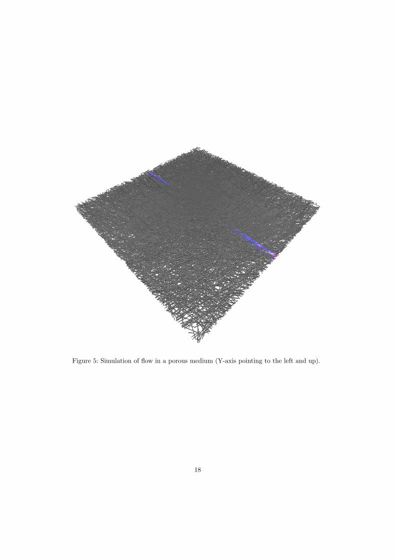
Figure 5: Simulation of flow in a porous medium (Y-axis pointing to the left and up).

18

Figure 6: Velocity profile of flow through a porous medium (lower picture shows the velocity profile only)

19

7 Free Surface Visualization

In a free surface simulation, waLBerla stores additional information regarding the free surface in interfacecells, which form a closed layer between liquid and gas phase. A detailed description of this concept canbe found in [Poh07]. Most important in the following are the free surface fill levels, the free surface pointsand the free surface normals. The fill levels store the amount of cell volume filled with liquid for eachcell. Cells with a fill level of 1 are liquid cells, and cells with a fill level of 0 are gas cells. From the filllevel information a surface point lying on the free surface and its surface normal in that point can beapproximated for every interface cell.

7.1 Free Surface Extraction

WaLBerla currently supports the following methods of creating POV-Ray visualizations from the freesurface data: The first method is to visualize the surface normals as glyphs starting from the calculatedfree surface points. This method thus directly shows what the free surface information calculated by thefree surface algorithm. With the second method waLBerla creates a closed triangle mesh from the filllevels that resembles the free surface. To do this the marching cubes algorithm from [LC87] is used. Thealgorithm proceeds through the field of fill levels and approximates intersection points of an iso surfacethrough a given threshold value in [0..1] with a cube of eight neighbored cells by linear interpolation.The intersection points can now be connected by a set of triangles lying within the cube. This is donein such a way that the triangles fuse together and form a closed surface. In order to add curvatureinformation to the triangle mesh, surface normals are calculated and stored for every triangle vertex. Thisis done by applying the linear interpolation scheme along the edges of the marching cube on the surfacenormals calculated for the respective cells. The resulting surface approximation translates directly into aPOV-Ray mesh2 object as described in the POV-Ray documentation [oVPL04]. According to waLBerla’spatch concept, which is introduced in [GDF+07b], the triangulation is done separately for every patch.The resulting triangle meshes from different patches are composed into one object during ray tracing. Thetriangulation process is implemented in the FSIsoSurface class, which reads the fill levels and the surfacenormals from the respective fields of a given patch. The free surface algorithm as described in [Poh07],however, only calculates surface normals for interface cells. Since during the triangulation the marchingcubes scheme interpolates along edges that connect to other celltypes, too, the normal calculation, whichis done in waLBerla’s FS NORMALS sweep had to be extended. Normals have to be constructed for allcells with a fill level above [below] the threshold value, if they have a neighbour with fill level below [above]the threshold value. Here a cell counts as neighbour only if it is connected to the original cell by an edgeof the marching cube.

7.2 Usage and Examples

To control the aspects of a free surface flow simulation there is a freesurface block in waLBerla’s param-eter files. The POV-Ray visualization of free surfaces is activated by simply adding a povvistype to thefreesurface block. The smoothsurface parameter can be used to control which of the two output meth-ods presented above will be used. If the keyword is present, a triangle mesh is written, the surface normalsotherwise. Every process will write its free surface output to the file ./dat/<pid>/FS<framenumber>.dat,where pid is the number of the process and framenumber is the number of the written time step. Thefiles are then composed to a POV-Ray union and added to the scene in the ./Globals.inc file.The following example suggests some materials suited for rendering free surface flows with POV-Ray.

Breaking Dam A standard test case in computational fluid dynamics is the breaking dam. This exam-ple shows how to visualize with POV-Ray such a flow simulated in waLBerla with the smoothSurfaceparameter set to 0.5. To give the simulated fluid a water like look, a fully transparent surface pigmentin combination with a highly specular finish was chosen for the free surface (see listing 11). With thissurface texture the free surface looks like a reflective transparent film. The POV-Ray manual [oVPL04]

20

describes finishes as well as the parameters stated in the following in detail. To make the liquid regionthat is enclosed by the free surface more distinctive from the outside region, an interior was assigned to thefree surface mesh. The ior (Index of Refraction) of 1.33, which is similar to the refraction index of water,controls the directional change of light rays passing when entering or leaving the object. The dispersionparameter additionally influences the refraction of light according to the color of the hitting light rays.Also the interior medium was defined to be absorbing red and green light, which gives a blue - coloredliquid.

Listing 11: POV-Ray material for the free surface

#dec l a r e FreeSur face = texture{pigment{

rgbt <0, 0 , 0 , 1>}

f i n i s h {ambient 0 .05d i f f u s e 0 .25b r i l l i a n c e 6 .0phong 0 .8phong s i ze 120r e f l e c t i o n { 0 .01 , 0 .7 }

}}

#dec l a r e WaterInt = i n t e r i o r {i o r 1 .33d i s p e r s i on 1 .05media{

absorpt ion <0.05 ,0.05 ,0 >}

}

To create a caustic effect, i.e. light being reflected and refracted by the free surface, photon mappingwas used, which is controlled by the photons block in the SDL file or the parameter file respectively. Fora highly reflective object such as a free surface, the collect option should always be turned off. Note, thatphoton rendering of objects is only done if it is activated in POV-Rays global settings (See [oVPL04]).Listing 12 shows the visualization type used for the free surface. It is important to declare the object ashollow. Otherwise POV-Ray skips the rendering of the interior of the object.

Listing 12: Visualization type for the free surfacePovVisType{ // water ( f r e e su r f a c e )

id 2 ;t exture FreeSur face ;i n t e r i o r WaterInt ;hol low ;photons{

t a rg e t ;r e f l e c t i o n ;r e f r a c t i o n ;// c o l l e c t ;

}}

21

Figure 7: Breaking dam.

22

8 Conclusion

In this paper we presented some possibilities to visualize CFD data from waLBerla with the POV-Ray raytracer. The waLBerla framework supports a wide range of applications addressing different kinds of fluiddynamic problems. These include different kinds of obstacles and complex geometries, particle flows andmoving objects, as well as free surface flows. All of the mentioned applications are integrated in a flexiblemanner such that they can be modularly combined with different debugging, analysis and visualizationmodules, consistently optimized for large-scale parallel simulations. Hence, also the proposed POV-Raymodule is integrated in a generic way to support various visualization possibilities for all existing andfuture applications.

While lacking the interactivity and flexibility of commonly used visualization toolkits, ray tracing canstill yield very convincing results which becomes especially apparent when dealing with free surface flows.Here, two techniques have been implemented, one using glyphs, directly showing the computed dataand designed for assisting debugging, and one for presentation purposes. There is also the possibility tovisualize the macroscopic field values of a simulated flow directly, e.g., by using a color map to show thedensity or velocity of the flow. For moving objects, the pathways can be tracked and the acting forces canbe visualized.

The waLBerla interface as presented in this paper provides a priori control of most output features.However, the POV-Ray output generated by waLBerla has been structured in a flexible manner, thatallows the modification of many visualization aspects of a simulation by modifying a single file even forparallel simulation setups.

23

References

[DGF+07] S. Donath, J. Gotz, C. Feichtinger, K. Iglberger, S. Bergler, and U. Rude, On the ResourceRequirements of the Hyper-Scale waLBerla Project, Tech. Report 07–13, Chair for SystemSimulation, Univ. of Erlangen, Sep 2007, http://www10.informatik.uni-erlangen.de/Publications/TechnicalReports/TechRep07-13.pdf.

[GDF+07a] J. Gotz, S. Donath, Ch. Feichtinger, K. Iglberger, and U. Rude, Concepts of walberla prototype0.0, Tech. Report 07–04, 2007.

[GDF+07b] , Concepts of walberla prototype 0.1, Tech. Report 07–10, 2007.

[GFI+08] J. Gotz, C. Feichtinger, K. Iglberger, S. Donath, and U. Rude, Large scale simulation of fluidstructure interaction using lattice Boltzmann methods and the ‘physics engine’, Proceedingsof CTAC 2008 (Geoffry N. Mercer and A. J. Roberts, eds.), ANZIAM J., vol. 50, 2008,pp. C166–C188.

[LC87] William E. Lorensen and Harvey E. Cline, Marching cubes: A high resolution 3d surfaceconstruction algorithm, Computer Graphics 21(4) (1987).

[oVPL04] Persistence of Vision Pty. Ltd., Persistence of vision (tm) raytracer, 2004, http://www.povray.org.

[Par09] ParaView, Information on visualization tool ParaView, available at http://www.paraview.org/, August 2009.

[Poh07] T. Pohl, High performance simulation of free surface flows using the lattice boltzmann method,Ph.D. thesis, University of Erlangen-Nuremberg, Lehrstuhl fur Informatik 10 (Systemsimu-lation), Institut fur Informatik, 2007.

[VTK09] VTK, Information on VTK, the Visualization Tool Kit, available at http://www.vtk.org/,August 2009.

24