legend given some polygons (“obstacles”) in the plane, a ...alubiw/cs763/lecture15.pdf · phy...
TRANSCRIPT
CS 763 F16 A. Lubiw, U. WaterlooLecture 15: Shortest Paths
Shortest paths in the plane with polygonal obstacles
UNIVERSITY A
VENUE WEST SEAGRAM DRIVE
COLUMBIA STREET WEST
RING ROAD
Campus Court
University ShopsPlaza
WELLESLEYCOURT
EBY HALL BECK HALL
WOOLWICHCOURTWATERLOO
COURT
WILMOTCOURT
PLAYING FIELDS
VILLAGE GREENW
ESTM
OU
NT
RO
AD
NO
RTH
LAU
REL
CREE
K
PHIL
LIP
STR
EET
PHIL
LIP
STR
EET
RING R
OAD
WES GRAHAM WAY WES GRAHAM WAY
FRANK TOMPA DRIVE FRANK TOMPA DRIVE
HA
GEY
BO
ULE
VAR
D
COLUMBIA LAKE
LAURELLAKE
WES
TMO
UNT
RO
AD
NO
RTH
HumanitiesTheatre
Theatreof the Arts
WEATHERSTATION
HAGEYBOULEVARD
Warrior Field
UW Police andParking Services
Visitors CentreCampus Tours
SEAGRAM DRIVE
SUN
VIE
W S
TREE
T
LEST
ER S
TREE
T
C
V S JK
P
PP
P
M
N
OVW
XX
R
L
O
B
T
H
A
D
EC
P
P
CL
HV
UWP
300
445
375
340
275
DAVID JOHNSTON RESEARCH + TECHNOLOGY PARK
ACWCLN
CLV
REVTH
MKV
V1
FED
UC
PAC
SLC
HS
REN
MHR
PAS
EV2
EV3
EV1
HH
AL
MLRCH
PHY
B1
ESC
MCC2
DCECH
EITB2
QNC
CPH
UWP
E2
E3
E5
EC3 EC1
EC2
E6
M3
NH LIB
TC
GH
SCH
DWESTP
STJ
CGR
LHIERC
CIFOPT
KDC
HMNBRH
RA2RAC
BAU
CSBCOM
GSC
BMH
COG
WCP
BUILDING INDEXCODE BUILDING – LOCATIONACW Accelerator Centre – G1AL Arts Lecture Hall – G4B1 Biology 1 – G4B2 Biology 2 – G4BMH B.C. Matthews Hall – G3BRH Brubacher House – F2C2 Chemistry 2 – G3, G4CGR Conrad Grebel University College – F5CIF Columbia Icefield – G2CLN Columbia Lake Village North – B2, C1, C2CLV Columbia Lake Village – B2, C2, D2COG Columbia Greenhouses – D2COM Commissary – H3
CPH Carl A. Pollock Hall – H4CSB Central Services Building – G3DC William G. Davis Computer Research Centre –
H3, H4DWE Douglas Wright Engineering Building – H4E2 Engineering 2 – H4E3 Engineering 3 – H4E5 Engineering 5 – H3, H4E6 Engineering 6 – H4EC1 East Campus 1 – I3EC2 East Campus 2 – H3EC3 East Campus 3 – H3ECH East Campus Hall – H3, H4, I3, I4EIT Centre for Environmental & Information
Technology – G4ERC Energy Research Centre – G3
EV1 Environment 1 – G5EV2 Environment 2 – G5EV3 Environment 3 – G5ESC Earth Sciences & Chemistry – G4FED Federation Hall – F3GA 335 Gage Street – see back pageGH Graduate House – G4GSC General Services Complex – G3, H3HH J.G. Hagey Hall of the Humanities – G5 HMN Hildegard Marsden Nursery – G2HS Health Services – F4KDC Klemmer Day Care – G2LHI Lyle S. Hallman Institute for Health Promotion – G3LIB Dana Porter Library – G4M3 Mathematics 3 – G3
MC Mathematics & Computer Building– G3MHR Minota Hagey Residence – F5, G5MKV William Lyon Mackenzie King Village – E3ML Modern Languages – G4NH Ira G. Needles Hall – G4OPT School of Optometry – G2PAC Physical Activities Complex – G3PAS Psychology, Anthropology, Sociology – G5PHR School of Pharmacy – see back pagePHY Physics – G4, H4QNC Mike & Ophelia Lazaridis Quantum-Nano Centre – G4RAC Research Advancement Centre – F1RA2 Research Advancement Centre 2 – F1RCH J.R. Coutts Engineering Lecture Hall – H4
REN Renison University College – F4REV Ron Eydt Village – E3SCH South Campus Hall – G4, G5, H5SLC Student Life Centre – G3STJ St. Jerome’s University – F4STP St. Paul’s University College – F4TC William M. Tatham Centre for Co-operative Education & Career Action – G4, G5TH Tutors’ Houses – E3UC University Club – F3UWP University of Waterloo Place – I4, I5V1 Student Village 1 – E3, F3
PARKING INDEXVISITOR PARKINGAll Day, Every DayC, N, W, X: $5 per day – pay and display Lot X is free on weekendsHV: Weekdays: $2 per hour up tp daily maximum of $15. After 5 p.m. and weekends: $5 coin entryM: $6 pay and displayD: Weekdays: $2 per hour up to daily maximum of $15. After 5 p.m. and weekends: $5 coin entryP: $4 coin entry for St. Jerome’s University, Renison University College; $5 coin entry for St. Paul’s University College; $1 per hour up to a $4 daily maximum at Conrad Grebel University CollegeOV: $5 coin exitJ, S, V: $5 pay and display. Pay in lot SCL, UWP: $5 pay and display
AFTER 4 P.M. AND WEEKENDSA, B, EC, H, R: $5 coin entry
PERMIT PARKING Faculty and Staff: A, B, H, K, L, N, O, R, T, XResident: CL, J, S, V, UWP, T Parking in any ungated lot after 4:30 pm with valid Faculty/Staff Permit
MOTORCYCLESPurchase a term or day pass from Parking Services, in the COM building for use at motorcycle pads
ACCESSIBLE PARKINGAccessible parking for persons with disabilities is available in most lots. For details visit:uwaterloo.ca/parking
SHORT-TERM PARKINGFifteen minute parking is available on the Ring Road at Environment 2 and Ira G. Needles Hall. Meter parking is available, visit the Parking website for locations at: uwaterloo.ca/parking
WATCARD PAYMENTAvailable at Lot C, N, W, X, M, UWP
LEGENDPARKING
Accessible Parking
Meter Parking
Motorcycle Parking
Permit Parking
Short-term Parking
Visitor Parking
COLOUR CODES
Academic/Administrative Buildings
Roads and Parking Lots
City Roads and Parking Lots
Pathways
Residence Buildings
Water
Research Park Buildings
P
SYMBOLS
Accessible Entrances
Building Codes
Construction Site and Future Site of Building
Grand River CarShare
Grand River Transit
Greyhound
GO Transit
Help Line Telephone
Information
Public Telephone
Service Vehicle
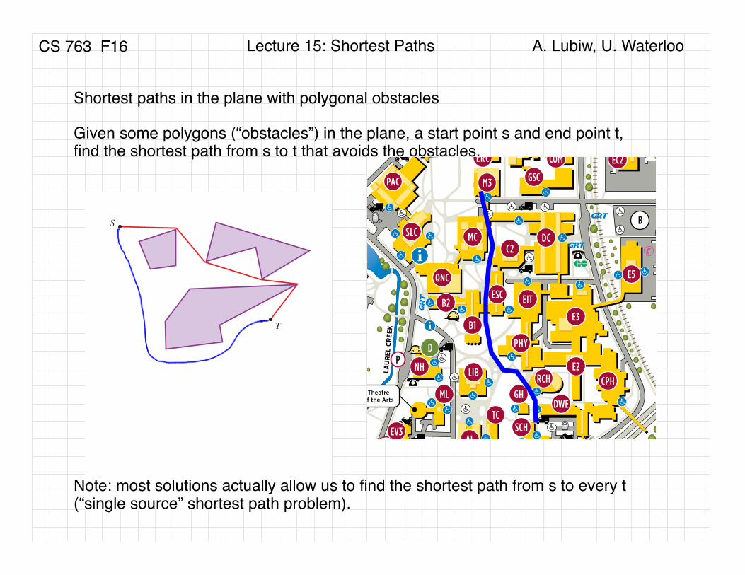
Given some polygons (“obstacles”) in the plane, a start point s and end point t, find the shortest path from s to t that avoids the obstacles.
T
S
Note: most solutions actually allow us to find the shortest path from s to every t(“single source” shortest path problem).
CS 763 F16 A. Lubiw, U. WaterlooLecture 15: Shortest Paths
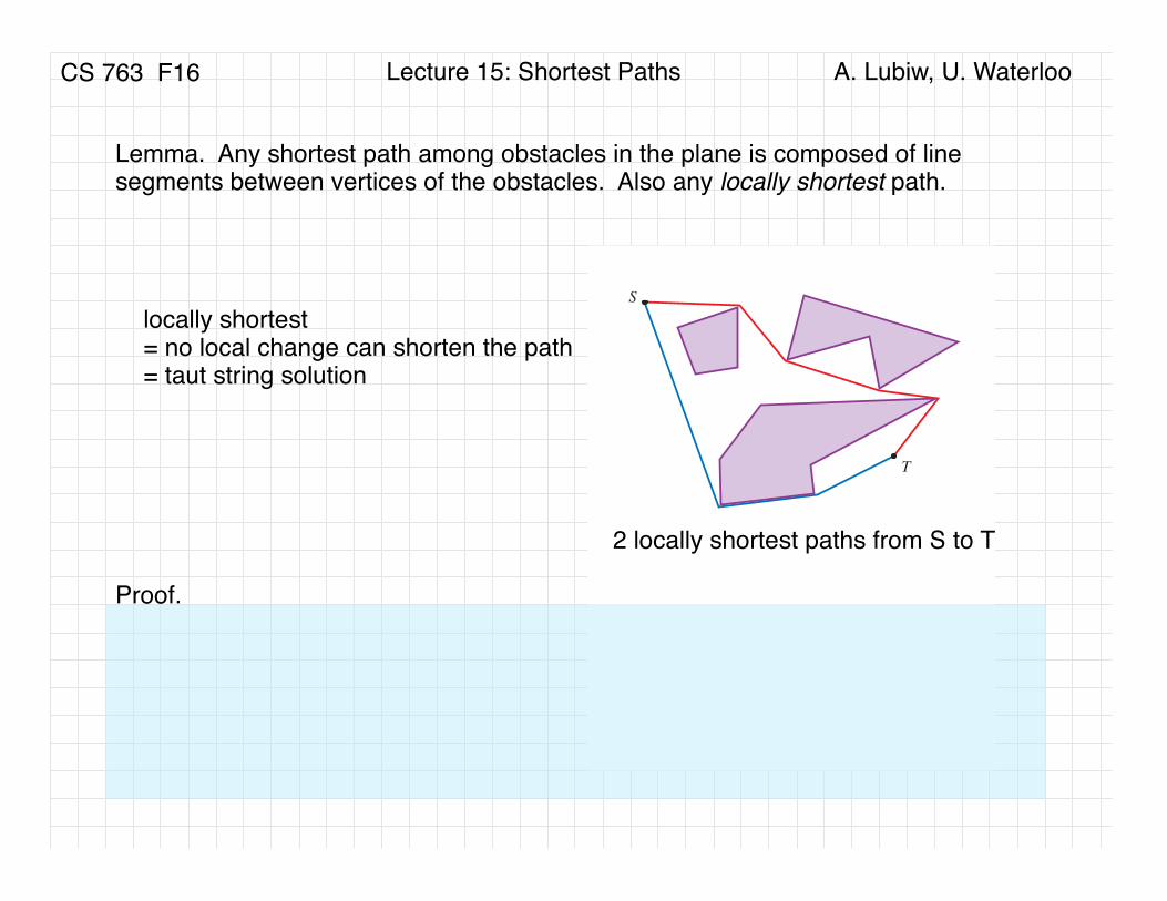
Lemma. Any shortest path among obstacles in the plane is composed of line segments between vertices of the obstacles. Also any locally shortest path.
T
S
Proof.
2 locally shortest paths from S to T
locally shortest = no local change can shorten the path= taut string solution
CS 763 F16 A. Lubiw, U. WaterlooLecture 15: Shortest Paths
S
T
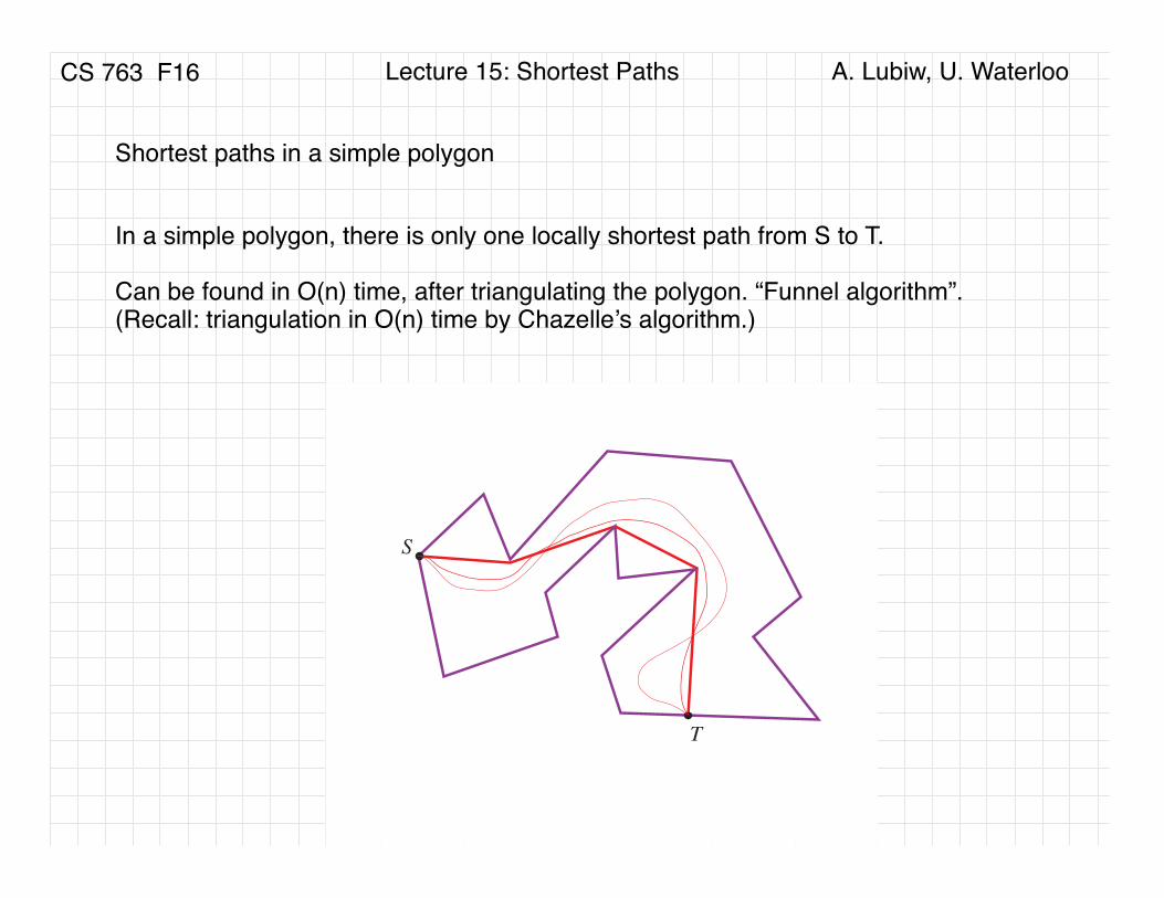
Shortest paths in a simple polygon
In a simple polygon, there is only one locally shortest path from S to T.
Can be found in O(n) time, after triangulating the polygon. “Funnel algorithm”. (Recall: triangulation in O(n) time by Chazelle’s algorithm.)
CS 763 F16 A. Lubiw, U. WaterlooLecture 15: Shortest Paths
Shortest paths in the plane with polygonal obstacles
T
S
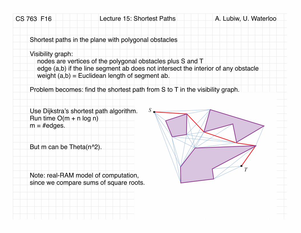
Visibility graph: nodes are vertices of the polygonal obstacles plus S and Tedge (a,b) if the line segment ab does not intersect the interior of any obstacleweight (a,b) = Euclidean length of segment ab.
Problem becomes: find the shortest path from S to T in the visibility graph.
Use Dijkstra’s shortest path algorithm.Run time O(m + n log n)m = #edges.
Note: real-RAM model of computation, since we compare sums of square roots.
But m can be Theta(n^2).
CS 763 F16 A. Lubiw, U. WaterlooLecture 15: Shortest Paths
Computing the visibility graph.
Obvious: O(n^3)Plane sweep: O(n^2 log n)Line arrangements: O(n^2)
Output sensitive: O(n log n + k), k = output size = number of edges of vis. graph. [Ghosh and Mount, 1991]. Huge efforts went into this line of research, but the bottleneck is that the visibility graph can have n^2 edges.
The O(n^2) algorithm via line arrangements [Welzl, 1985]described for non-degenerate disjoint line segments.

CS 763 F16 A. Lubiw, U. WaterlooLecture 15: Shortest Paths
reminder of Dijkstra’s algorithm

CS 763 F16 A. Lubiw, U. WaterlooLecture 15: Shortest Paths
geometric visualization of Dijkstra’s algorithm — imagine paint flowing along edges
CS 763 F16 A. Lubiw, U. WaterlooLecture 15: Shortest Paths
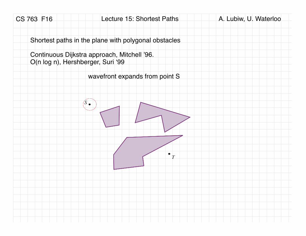
Shortest paths in the plane with polygonal obstacles
Continuous Dijkstra approach, Mitchell ’96. O(n log n), Hershberger, Suri ‘99
wavefront expands from point S
CS 763 F16 A. Lubiw, U. WaterlooLecture 15: Shortest Paths
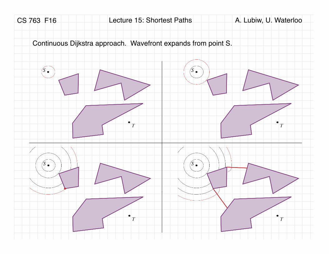
Continuous Dijkstra approach. Wavefront expands from point S.
CS 763 F16 A. Lubiw, U. WaterlooLecture 15: Shortest Paths
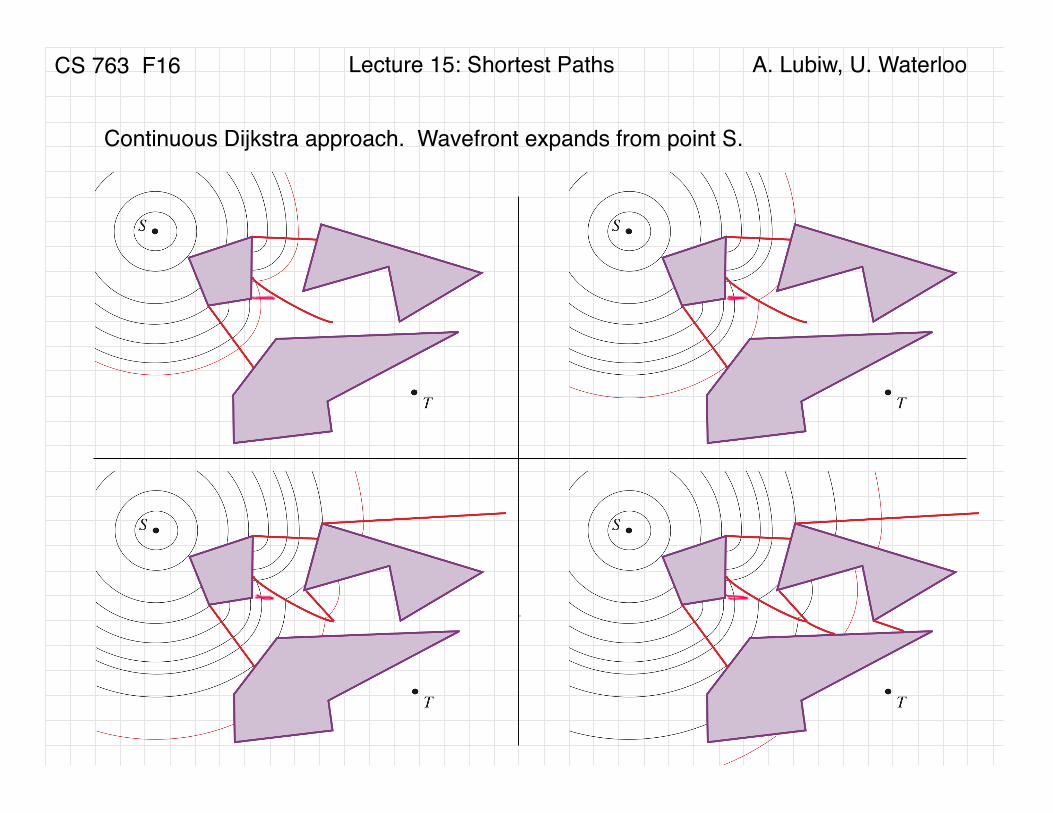
Continuous Dijkstra approach. Wavefront expands from point S.

CS 763 F16 A. Lubiw, U. WaterlooLecture 15: Shortest Paths
Continuous Dijkstra approach.
Implementation issues:
- keep track of events where the wave front changes combinatorially
- find which event occurs next (use a priority queue)
- make updates for that event
Original version was O(n^2 log n).
Improved to O(log n) by Hershberger, Suri
502 Discrete Comput Geom (2008) 39: 500–579
and Han follow the general idea of Mount [28] to solve the problem of storing short-
est path information separately, for a general, possibly nonconvex polyhedral surface.
They obtain a tradeoff between query time O (d log n / logd ) and space complex-ity O (n log n / logd ), where d is an adjustable parameter. Again, the question whetherthis data structure can be constructed in subquadratic time, has been left open.
The problem has been more or less “stuck” after Chen and Han’s paper, and the
quadratic-time barrier seemed very difficult to break. For this and other reasons, sev-
eral works [2–4, 16, 17, 19, 24, 25, 38] presented approximate algorithms for the
3-dimensional shortest path problem. Nevertheless, the major problem of obtain-
ing a subquadratic, or even near-linear, exact algorithm remained open. In 1999,
Kapoor [21] announced such an algorithm for the shortest path problem on an ar-
bitrary polyhedral surface P (see also a review of the algorithm in O’Rourke’s col-
umn [29]). The algorithm follows the continuous Dijkstra paradigm, and claims to be
able to compute a shortest path between two given points in O (n log2 n) time (so itdoes not preprocess the surface for answering shortest path queries). However, as far
as we know, the details of Kapoor’s algorithm have not yet been published.
The Algorithm of Hershberger and Suri for Polygonal Domains A dramatic break-
through on a loosely related problem took place in 1995,1 when Hershberger and
Suri [18] obtained an O (n log n)-time algorithm for computing shortest paths in theplane in the presence of polygonal obstacles (where n is the number of obstacle ver-tices). The algorithm actually computes a shortest path map from a fixed source point
to all other (non-obstacle) points of the plane, which can be used to answer single-
source shortest path queries in O (log n) time.Our algorithm uses (adapted variants of) many of the ingredients of [18], includ-
ing the continuous Dijkstra method—in [18], the wavefront is propagated amid the
obstacles, where each wave emanates from some obstacle vertex already covered by
the wavefront; see Fig. 1(a).
The key new ingredient in [18] is a quad-tree-style subdivision of the plane, of
size O (n), on the vertices of the obstacles (temporarily ignoring the obstacle edges).
Fig. 1 The planar case: (a) The wavefront propagated from s, at some fixed time t . (b) The conformingsubdivision of the free space
1A preliminary (symposium) version has appeared in 1993; the last version was published in 1999.
Schreiber & Sharir
complicated!
involves subdividing space and approximating the wavefront cell by cell
CS 763 F16 A. Lubiw, U. WaterlooLecture 15: Shortest Paths
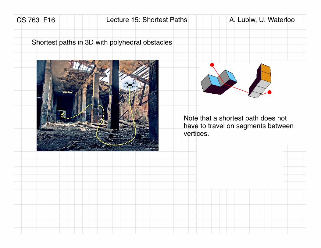
Shortest paths in 3D with polyhedral obstacles
Note that a shortest path does not have to travel on segments between vertices.
CS 763 F16 A. Lubiw, U. WaterlooLecture 15: Shortest Paths
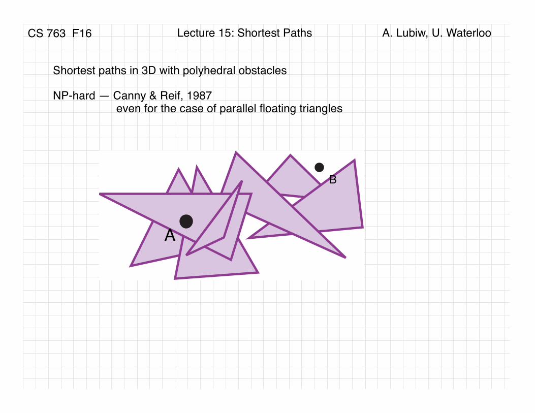
Shortest paths in 3D with polyhedral obstacles
A
B
NP-hard — Canny & Reif, 1987 even for the case of parallel floating triangles
CS 763 F16 A. Lubiw, U. WaterlooLecture 15: Shortest Paths
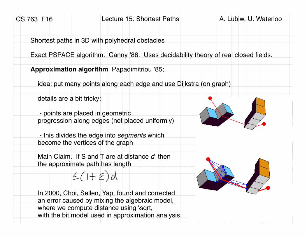
Shortest paths in 3D with polyhedral obstacles
Approximation algorithm. Papadimitriou ’85;
Exact PSPACE algorithm. Canny ’88. Uses decidability theory of real closed fields.
idea: put many points along each edge and use Dijkstra (on graph)
details are a bit tricky: - points are placed in geometric progression along edges (not placed uniformly)
- this divides the edge into segments whichbecome the vertices of the graph
Main Claim. If S and T are at distance d thenthe approximate path has length
In 2000, Choi, Sellen, Yap, found and correctedan error caused by mixing the algebraic model,where we compute distance using \sqrt,with the bit model used in approximation analysis
CS 763 F16 A. Lubiw, U. WaterlooLecture 15: Shortest Paths
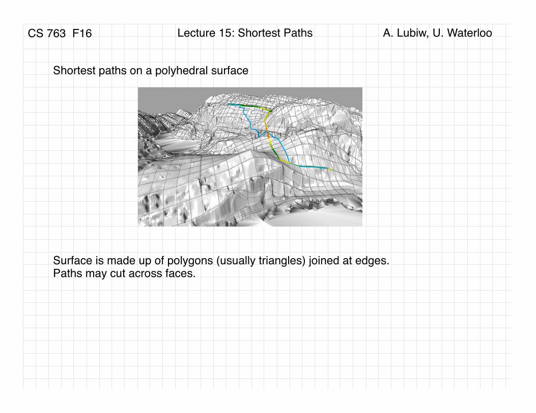
Shortest paths on a polyhedral surface
Surface is made up of polygons (usually triangles) joined at edges.Paths may cut across faces.

CS 763 F16 A. Lubiw, U. WaterlooLecture 15: Shortest Paths
Copyright © 2005 by the Association for Computing Machinery, Inc. Permission to make digital or hard copies of part or all of this work for personal or classroom use is granted without fee provided that copies are not made or distributed for commercial advantage and that copies bear this notice and the full citation on the first page. Copyrights for components of this work owned by others than ACM must be honored. Abstracting with credit is permitted. To copy otherwise, to republish, to post on servers, or to redistribute to lists, requires prior specific permission and/or a fee. Request permissions from Permissions Dept, ACM Inc., fax +1 (212) 869-0481 or e-mail [email protected]. © 2005 ACM 0730-0301/05/0700-0553 $5.00
Fast Exact and Approximate Geodesics on MeshesVitaly Surazhsky
University of OsloTatiana Surazhsky
University of OsloDanil KirsanovHarvard University
Steven J. GortlerHarvard University
Hugues HoppeMicrosoft Research
AbstractThe computation of geodesic paths and distances on trianglemeshes is a common operation in many computer graphics applica-tions. We present several practical algorithms for computing suchgeodesics from a source point to one or all other points efficiently.First, we describe an implementation of the exact “single source,all destination” algorithm presented by Mitchell, Mount, and Pa-padimitriou (MMP). We show that the algorithm runs much fasterin practice than suggested by worst case analysis. Next, we extendthe algorithm with a merging operation to obtain computationallyefficient and accurate approximations with bounded error. Finally,to compute the shortest path between two given points, we use alower-bound property of our approximate geodesic algorithm to ef-ficiently prune the frontier of the MMP algorithm, thereby obtain-ing an exact solution even more quickly.
Keywords: shortest path, geodesic distance.
1 IntroductionIn this paper we present practical methods for computing both exactand approximate shortest (i.e. geodesic) paths on a triangle mesh.These geodesic paths typically cut across faces in the mesh and aretherefore not found by the traditional graph-based Dijkstra algo-rithm for shortest paths.The computation of geodesic paths is a common operation in manycomputer graphics applications. For example, parameterizing amesh often involves cutting the mesh into one or more charts(e.g. [Krishnamurthy and Levoy 1996; Sander et al. 2003]), andthe result generally has less distortion and better packing efficiencyif the cuts are geodesic. Geodesic paths are used in segmenting amesh into subparts, as done in [Katz and Tal 2003; Funkhouser et al.2004]. Mesh editing systems such as [Kobbelt et al. 1998] also usegeodesics to delineate the extents of editing operations. Simulatingfire on a mesh [Lee et al. 2001] also benefits from geodesics.In addition, geodesic paths establish a surface distance metric,which is an essential building block for many other techniques. Forexample, radial-basis interpolation over a mesh requires calcula-tion of geodesic distances, and is used in numerous applicationssuch as skinning [Sloan et al. 2001], mesh watermarking [Praunet al. 1999], and the definition of surface vector fields [Praun et al.2000]. Shape classification algorithms such as [Hilaga et al. 2001]use Morse analysis of a geodesic distance field. Parameterizationmetrics based on isomaps [Zigelman et al. 2002; Zhou et al. 2004;Peyre and Cohen 2005] are also driven by geodesic distances.In this paper we explore the problem of producing both exact andapproximate solutions for geodesic paths (and hence distances) ontriangle meshes (Figure 1). We present three contributions:Exact algorithm We first present an efficient implementation ofthe exact geodesic algorithm by Mitchell, Mount, and Papadim-itriou (MMP) [1987]. Using a simple parameterization of the dis-
Figure 1: Geodesic paths from a source vertex, and isolines of thegeodesic distance function.
tance function over the edges, the implementation is actually prac-tical even though, to our knowledge, it has never been done pre-viously. We demonstrate that the algorithm’s worst case runningtime of O(n2 log n) is pessimistic, and that in practice, the algo-rithm runs in sub-quadratic time. For instance, we can computethe exact geodesic distance from a source point to all vertices of a400K-triangle mesh in about one minute.Approximation algorithm We extend the algorithm with a merg-ing operation to obtain computationally efficient and accurate ap-proximations with bounded error. In practice, the algorithm runs inO(n log n) time even for small error thresholds.Exact geodesic path between two points We show how toefficiently obtain the exact solution to the “single source, singledestination” problem, by using a lower-bound property of our ap-proximation algorithm to prune the frontier of the MMP algorithm.In practice, we compute the shortest path between two points on a1M-triangle mesh in just a few seconds.
2 Related workThe MMP algorithm [Mitchell et al. 1987] provides an exact solu-tion for the “single source, all destination” shortest path problemon a triangle mesh. Their algorithm partitions each mesh edge intoa set of intervals (windows) over which the exact distance compu-tation can be performed atomically. These windows are propagatedin a “continuous Dijkstra”-like manner. They prove a worst caserunning time of O(n2 log n). Unfortunately, as far as we know theMMP algorithm has not been implemented previously and thus hasnot made its way into practice.An exact geodesic algorithm with worst case time complexity ofO(n2) was described by Chen and Han [1996] and partially imple-mented by Kaneva and O’Rourke [2000]. We show that our MMPimplementation runs many times faster than that implementation.Kapoor [1999] describes an algorithm for the “single source, sin-gle destination” geodesic path between two given mesh vertices,in O(n log2 n) time. This is a complicated method which calls assubroutines many other complicated computational geometry algo-rithms; it is unclear if this algorithm will ever be realized.Approximate geodesics with guaranteed error bounds can be ob-tained by adding extra edges into the mesh and running Dijkstraon the one-skeleton of this augmented mesh [Lanthier et al. 1997].
553
Fast Exact and Approximate Geodesics on MeshesSIGRAPH 2005
includes shortest paths on surface of polyhedron

CS 763 F16 A. Lubiw, U. WaterlooLecture 15: Shortest Paths
T
S
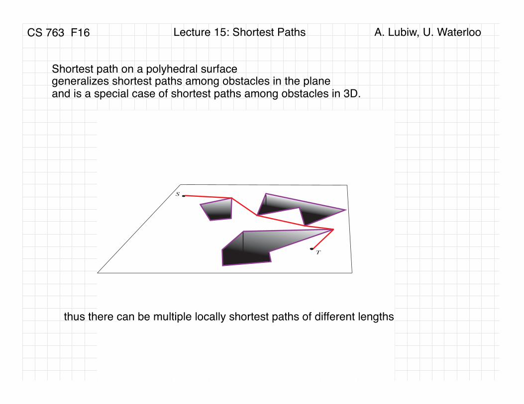
generalizes shortest paths among obstacles in the planeand is a special case of shortest paths among obstacles in 3D.
Shortest path on a polyhedral surface
T
S
CS 763 F16 A. Lubiw, U. WaterlooLecture 15: Shortest Paths
generalizes shortest paths among obstacles in the planeand is a special case of shortest paths among obstacles in 3D.
Shortest path on a polyhedral surface
thus there can be multiple locally shortest paths of different lengths
CS 763 F16 A. Lubiw, U. WaterlooLecture 15: Shortest Paths
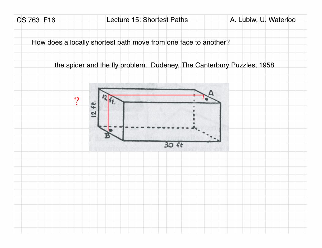
How does a locally shortest path move from one face to another?
?
the spider and the fly problem. Dudeney, The Canterbury Puzzles, 1958
CS 763 F16 A. Lubiw, U. WaterlooLecture 15: Shortest Paths
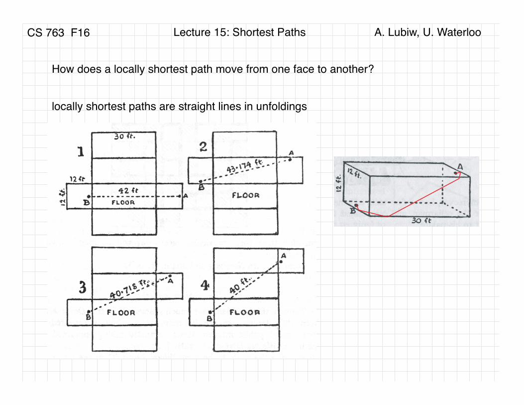
How does a locally shortest path move from one face to another?
locally shortest paths are straight lines in unfoldings
CS 763 F16 A. Lubiw, U. WaterlooLecture 15: Shortest Paths
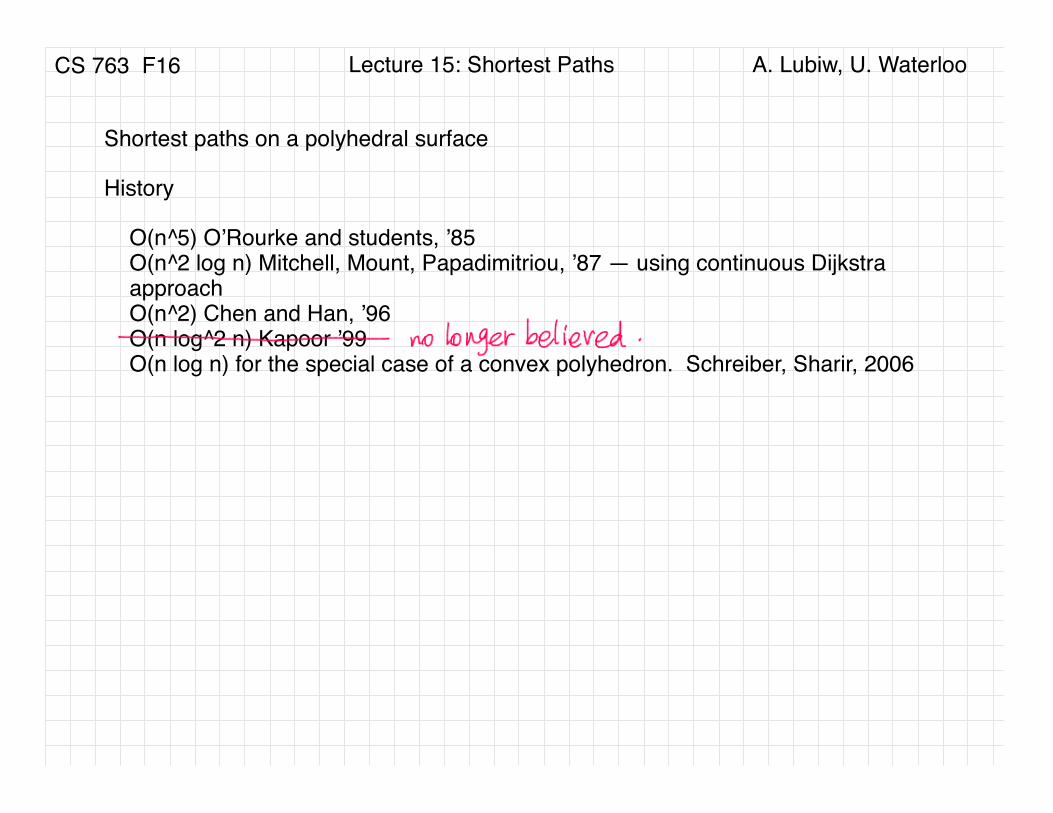
Shortest paths on a polyhedral surface
History
O(n^5) O’Rourke and students, ’85O(n^2 log n) Mitchell, Mount, Papadimitriou, ’87 — using continuous Dijkstra approachO(n^2) Chen and Han, ’96O(n log^2 n) Kapoor ’99O(n log n) for the special case of a convex polyhedron. Schreiber, Sharir, 2006
CS 763 F16 A. Lubiw, U. WaterlooLecture 15: Shortest Paths
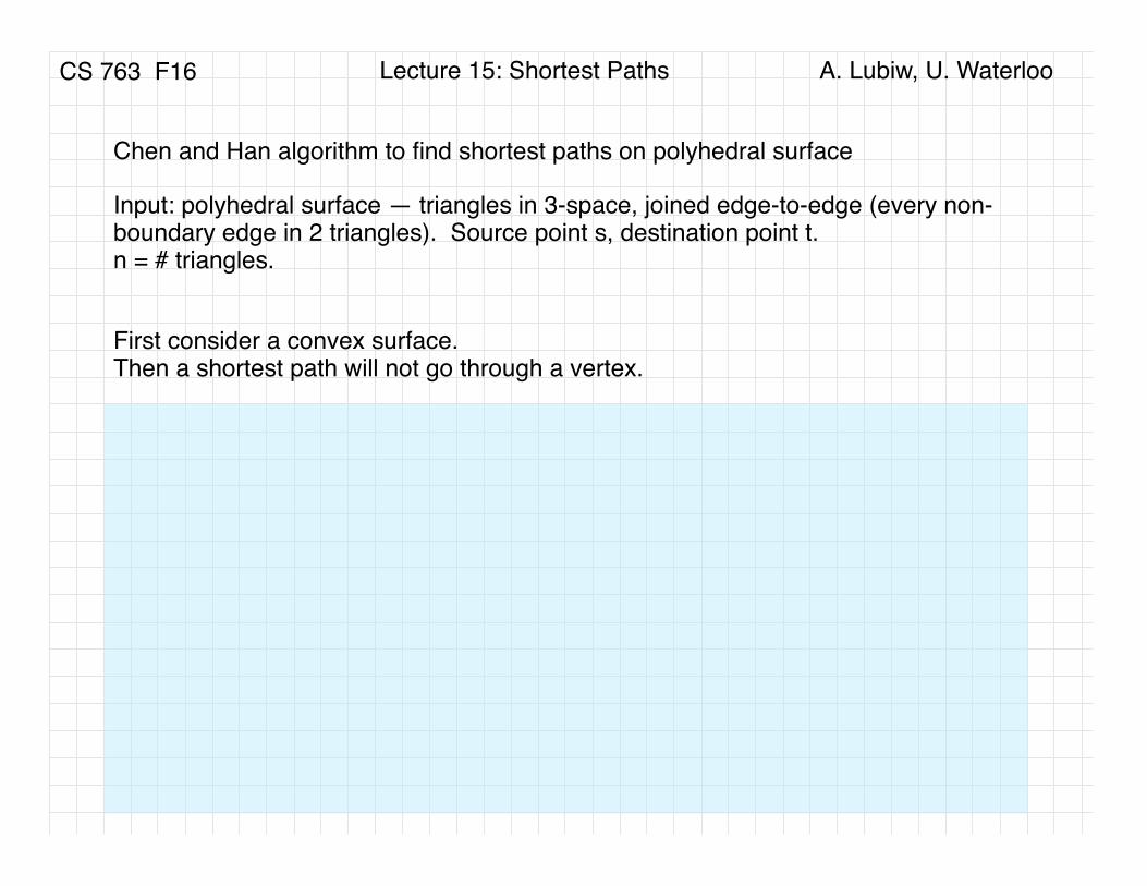
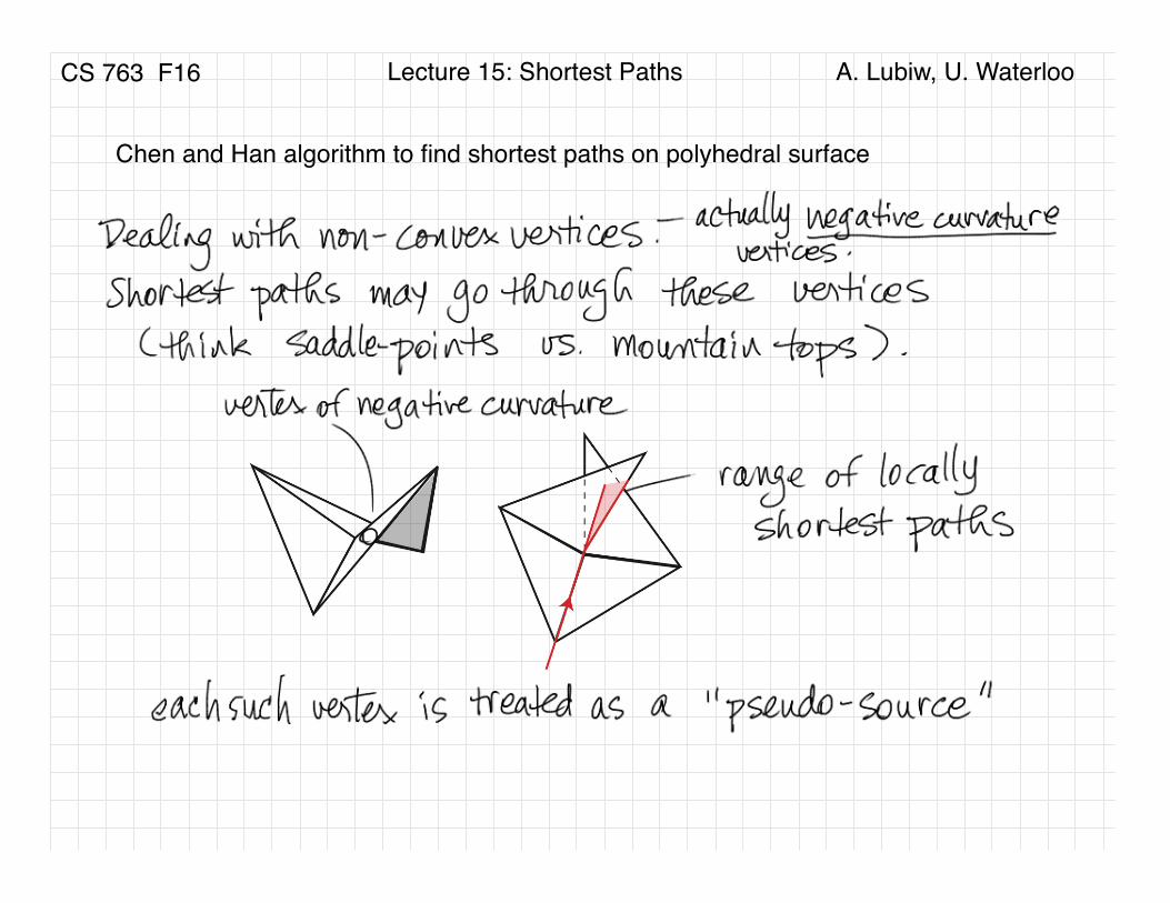
Chen and Han algorithm to find shortest paths on polyhedral surface
Input: polyhedral surface — triangles in 3-space, joined edge-to-edge (every non-boundary edge in 2 triangles). Source point s, destination point t.n = # triangles.
First consider a convex surface.Then a shortest path will not go through a vertex.
CS 763 F16 A. Lubiw, U. WaterlooLecture 15: Shortest Paths
Chen and Han algorithm to find shortest paths on polyhedral surface
CS 763 F16 A. Lubiw, U. WaterlooLecture 15: Shortest Paths
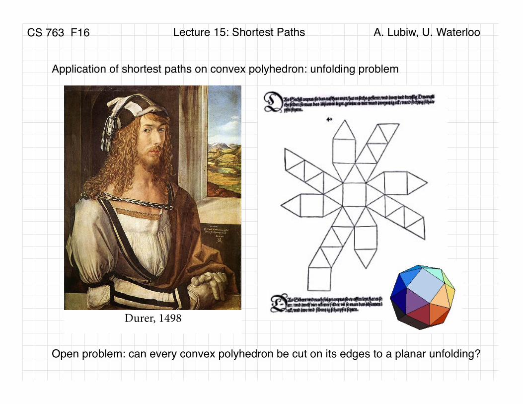
Application of shortest paths on convex polyhedron: unfolding problem
Durer, 1498
Open problem: can every convex polyhedron be cut on its edges to a planar unfolding?

CS 763 F16 A. Lubiw, U. WaterlooLecture 15: Shortest Paths
Application of shortest paths on convex polyhedron: unfolding problem unfolding was introduced by Alexandrov in 1948 [Ale50, p. 181][Ale05, p. 195]1but only proved to avoid overlap more recently [AO92].
If P has n vertices, the unfolding has 2n vertices, n of which are images ofx, which alternate with the n images of the vertices of P. Because x can be anygeneric point on the surface (and there is only a finite network of nongenericpoints to avoid), the star unfolding provides an entire class of unfoldings for agiven P.
F
L
RT
F
Bt
Bt
Bk
Bk
Bt
FBt
Bt
Bk
Bt
Bt
Bt
(a) (b)
T
x
Bt
FR
L
Bk
Figure 8: (a) 2⇥1⇥1 box. Box faces are labeled: Bt,F,T,R,L,Bk for Bottom,Front, Top, Left, Right, and Back respectively. (b) Star unfolding with respectto x.
The second general unfolding for a convex polyhedron is the source unfolding.Again we start with a source point x 2 P, but this time we follow shortest paths�(x, y) from x to every point y 2 P. The closure of the set of points y suchthat �(x, y) is not unique forms the cut locus C(x) ⇢ P of x. The notion of cutlocus was introduced by Poincare in 1905 [Poi05], and since then has become acentral concept in global Riemannian geometry. Its name reflects the fact thatshortest paths are “cut” or terminated when they reach the cut locus. The cutlocus for the box example is shown in Figure 9(a). Notice that the cut locus isindeed a spanning tree of the vertices of P (this the reason for the closure in thedefinition). So cutting C(x) will enable flattening the surface. The resultingsource unfolding for the box example is shown in (b) of the figure. That this doesnot overlap is clear, because one can view it as composed of straight-segment“spokes” of length �(x, y) for each y 2 C(x), emanating around x at every angle.
Returning to the star unfolding, the cut locus C(x) unfolds to a tree in U
⇤(x)that spans the n vertices of U
⇤(x) which are the images of the vertices of P.
3.2 Nonconvex
Now that we have seen that all convex polyhedra have (many) general unfold-ings, it is natural to ask whether nonconvex polyhedra do also. Here again the
1And so sometimes called an “Alexandrov unfolding” [MP08].
7
F
Bt
Bk
L R
T
T
x
(a) (b)
x
Bt
F
R
TL
Bk
Figure 9: (a) 2⇥1⇥1 box, with cut locus C(x) marked. (b) Source unfoldingwith respect to x.
answer is unknown: there is neither a counterexample, nor a general algorithm.Progress has been made recently on orthogonal polyhedra.
3.2.1 Orthogonal Polyhedra
We saw one special class of orthogonal polyhedra that can be edge unfolded,and one example (Figure 3(b)) of an orthogonal polyhedron that cannot be edgeunfolded. However, if we permit ourselves arbitrary cuts, it is not di�cult tounfold this edge-ununfoldable example into a number of thin, connected strips.See Figure 10 for one way, the result of applying a variation on the algorithmfrom Section 1 for orthogonal terrains.
The idea of slicing an orthogonal polyhedron into strips was explored in aseries of papers handling special classes (summarized in [O’R08]), finally culmi-nating in an algorithm that unfolds any orthogonal polyhedron P (of genus zero)into a single, non-overlapping piece [DFO07]. This algorithm “peels” the sur-face into a thin strip, following a recursively-nested helical path on the surfaceof P. Although the cuts are arbitrary, they are parallel to polyhedron edges,which is natural in this context. Unfortunately, the resulting unfolding can beexponentially thin and exponentially long: if P has n vertices and has longestdimension 1, strips might have width 1/2O(n) and stretch out to length 2O(n).
4 Summary & Prospects
Table 1 summarizes the status of the main questions on unfolding.Of course there are many topics we have not discussed. For exam-
ple, the source and star unfoldings have been generalized to “quasigeodesic”
8
A Generalization of the Source Unfolding ofConvex Polyhedra
Erik D. Demaine1 and Anna Lubiw2
1 MIT Computer Science and Artificial Intelligence Laboratory, Cambridge, [email protected]
2 David R. Cheriton School of Computer Science, University of Waterloo, [email protected]
Dedicated to Ferran Hurtado on the occasion of his 60th birthday.
Abstract. We present a new method for unfolding a convex polyhedroninto one piece without overlap, based on shortest paths to a convex curveon the polyhedron. Our “sun unfoldings” encompass source unfoldingfrom a point, source unfolding from an open geodesic curve, and a variantof a recent method of Itoh, O’Rourke, and Vılcu.
1 Introduction
The easiest way to show that any convex polyhedron can be unfolded is via thesource unfolding from a point s, where the polyhedron surface is cut at the ridgetree of points that have more than one shortest path to s, [10], or see [3]. Theunfolding does not overlap because the shortest paths from s to every other pointon the surface develop to straight lines radiating from s, forming a star-shapedunfolding. See Figure 1(b).
(b)(a) (c)
C
Fig. 1. [based on O’Rourke [9]] Unfolding a box from a point on the middle of the base:(b) source unfolding with some shortest paths shown. The source unfolding is the sameas the sun unfolding relative to circle C. (c) star unfolding, with ridge tree shown.
Our main result is a generalized unfolding, called a sun unfolding, that pre-serves the property that shortest paths emanate in a radially monotone way,
Every convex polyhedron can be unfolded via the source and star unfolding
p
cut shortest path from x to every vertex cut Voronoi diagram of x (“ridge tree”) star unfolding source unfolding