1

A General Structure for Legal Arguments Using Bayesian Networks

Norman Fenton and Martin Neil

norman@eecs.qmul.ac.uk martin@eecs.qmul.ac.uk

School of Electronic Engineering and Computer Science

Queen Mary, University of London London E1 4NS

and

Agena Ltd

11 Main Street Caldecote Cambridge CB23 7NU

David Lagnado

d.lagnado@ucl.ac.uk Dept of Cognitive,

Perceptual and Brain Sciences University College London University College London

Gower St London WC1E 6BT

10 November 2010

2

Abstract

A Bayesian network (BN) is a graphical model of uncertainty that is especially well-suited to legal arguments. It enables us to visualise and model dependencies between different hypotheses and pieces of evidence and to calculate the revised probability beliefs about all uncertain factors when any piece of new evidence is presented. Although BNs have been widely discussed and recently used in the context of legal arguments there is no systematic, repeatable method for modelling legal arguments as BNs. Hence, where BNs have been used in the legal context, they are presented as completed pieces of work, with no insights into the reasoning and working that must have gone into their construction. This means the process of building BNs for legal arguments is ad-hoc, with little possibility for learning and process improvement. This paper directly addresses this problem by describing a method for building useful legal arguments in a consistent and repeatable way. The method complements and extends recent work by Hepler, Dawid and Leucari on objected-oriented BNs for complex legal arguments and is based on the recognition that such arguments can be built up from a small number of basic causal structures (referred to as idioms). We present a number of examples that demonstrate the practicality and usefulness of the method. The method also enables us to handle an apparent paradox observed in previous empirical studies, whereby it has been observed that people may reason about evidence in a ‘non-normative’ way, meaning that their conclusions conflict with the results of the associated causal BN. In particular, subjects exhibited such non-normative behaviour by asserting different probability beliefs when evidence was presented in a different order (whereas in a BN calculation the impact of evidence is not affected by the order in which the evidence is presented). By using the method presented in this paper we are able to show that the subjects were not necessarily reasoning irrationally. Rather, we are able to show that the order in which evidence is presented may require an alternative causal BN structure. Executable version of all of the BN models described in the paper are freely available for inspection and use (web link provided in paper). Keywords: legal arguments, probability, Bayesian networks Word count: 14,533

3

1 Introduction The role of probabilistic Bayesian reasoning in legal practice has been addressed in many articles and books such as [3] [17] [22] [23] [24] [27] [28] [31] [36] [47] [54] [55] [56] [57]. What we are especially interested in is the role of such reasoning to improve understanding of legal arguments. For the purposes of this paper an argument refers to any reasoned discussion presented as part of, or as commentary about, a legal case. It is our contention that a Bayesian network (BN), which is a graphical model of uncertainty, is especially well-suited to legal arguments. A BN enables us to visualise the relationship between different hypotheses and pieces of evidence in a complex legal argument. But, in addition to its powerful visual appeal, it has an underlying calculus that determines the revised probability beliefs about all uncertain variables when any piece of new evidence is presented. The proposal to use BNs for legal arguments is by no means new (see, for example, [5] [16] [35] [37] [60]). Indeed, in 1991 Edwards [19] provided an outstanding argument for the use of BNs in which he said of this technology:

“I assert that we now have a technology that is ready for use, not just by the scholars of evidence, but by trial lawyers.”

He predicted such use would become routine within “two to three years”. Unfortunately, he was grossly optimistic for reasons that are fully explained in [25]. One of the reasons for the lack of take up of BNs within the legal profession was a basic lack of understanding of probability and simple mathematics; but [25] described an approach (that has recently been used successfully in real trials) to overcome this barrier by enabling BNs to be used without lawyers and jurors having to understand any probability or mathematics. However, while this progress enables non-mathematicians to be more accepting of the results of BN analysis, there is no systematic, repeatable method for modelling legal arguments as BNs. In the many papers and books where such BNs have been proposed, they are presented as completed pieces of work, with no insights into the reasoning and working that must have gone into determining why the particular set of nodes and links between them were chosen rather than others. Also, there is very little consistency in style or language between different BN models even when they represent similar arguments. This all means that the process of building a BN for a legal argument is ad-hoc, with little possibility for learning and process improvement. The purpose of this paper is, therefore, to show that it is possible to meet the requirement for a structured method of building BNs to model legal arguments. The method we propose complements and extends recent work by Hepler, Dawid and Leucari [33]. The key contribution of [33] was to introduce the use of object-oriented BNs as a means of organising and structuring complex legal arguments. Hepler et al also introduced a small number of ‘recurrent patterns of evidence’, and it is this idea that we extend significantly in this paper, while accepting the object-oriented structuring as given. We refer to commonly recurring patterns as idioms. A set of (five) generic BN idioms was first introduced in [50]. These idioms represented an abstract set of classes of reasoning from which specific cases (called instances) for

4

the problem at hand could be constructed. The approach was inspired by ideas from systems engineering and systems theory and Judea Pearl’s recognition that: “Fragmented structures of causal organisations are constantly being assembled on the fly, as needed, from a stock of building blocks” [51] In this paper we focus on a set of instances of these generic idioms that are specific to legal arguments. We believe that the proposed idioms are sufficient in the sense that they provide the basis for most complex legal arguments to be built. Moreover, we believe that the development of a small set of reusable idioms reflects how the human mind deals with complex evidence and inference in the light of memory and processing constraints. The proposed idioms conform to known limits on working memory [12][32][48], and the reusable nature of these structures marks a considerable saving on storage and processing. The hierarchical structuring inherent in the general BN framework also fits well with current models of memory organization [20][30]. There is further support for this approach in studies of expert performance in chess, physics, and medical diagnosis, where causal schema and scripts play a critical role in the transition from novice to expert [10][21]. This fit with the human cognitive system makes the idiom-based approach particularly suitable for practical use by non-specialists. In contrast to Helpler et al., we emphasize the causal underpinnings of the basic idioms. The construction of the BNs always respects the direction of causality, even where the key inferences move from effect to cause. Again this feature meshes well with what is currently known about how people organize their knowledge and draw inferences [44][59]. Indeed the predominant psychological model of legal reasoning, the story model, takes causal schema as the fundamental building blocks for reasoning about evidence [52]. The building block approach means that we can use idioms to construct models incrementally whilst preserving interfaces between the model parts that ensure they can be coupled together to form a cohesive whole. Likewise, the fact that idioms contain causal information in the form of causal structure alone means any detailed consideration of the underlying probabilities can be postponed until they are needed, or we can experiment with hypothetical probabilities to determine the impact of the idiom on the case as a whole. Thus, the idioms provide a number of necessary abstraction steps that match human cognition and also ease the cognitive burden involved in engineering of complex knowledge-based systems. The idioms also enable us to address the important issue, highlighted in [41], that people may reason about evidence in a ‘non-normative’ way, meaning that their conclusions sometimes conflict with the results of the associated causal BN. In particular, under certain conditions subjects exhibited non-normative behaviour by asserting different probability beliefs when evidence was presented in a different order (whereas in a BN calculation the impact of evidence is not affected by the order in which the evidence is presented). By using the method presented in this paper we are able to show that the subjects were not necessarily reasoning irrationally. Rather, we show that the order in which evidence is presented may require an alternative causal BN structure.

5

The paper is structured as follows: In Section 2 we state our assumptions and notation, while also providing a justification for the basic Bayesian approach. The structured BN idioms are presented in Section 3, while examples of applying the method to complete legal arguments are presented in Section 4. We handle the difficult issue of order of evidence in Section 5. Our conclusions include a roadmap for empirical research on the impact of the idioms for improved legal reasoning. Executable versions of all of the BN models described in the paper are freely available for inspection and use at:

www.eecs.qmul.ac.uk/~norman/Models/legal_models.html 2 The basic case for Bayesian reasoning about evidence We start by introducing some terminology and assumptions that we will use throughout:

• A legal argument involves a collection of hypotheses and evidence about these hypotheses.

• A hypothesis is a Boolean statement whose truth value is generally unknowable to a jury. The most obvious example of a hypothesis is the statement “Defendant is guilty” (of the crime charged). Any hypothesis like this, which asserts guilt/innocence of the defendant, is called the ultimate hypothesis. There will generally be additional types of hypotheses considered in a legal argument, such as “defendant was present at the crime scene” or “the defendant had a grudge against the victim”.

• A piece of evidence is a Boolean statement that, if true, lends support to one or more hypothesis. For example, “an eye witness testifies that defendant was at scene of crime” is evidence to support the prosecution hypothesis that “defendant is guilty”, while “an eye witness testifies that the defendant was in a different location at the time of the crime” is evidence to support the defence hypothesis.

• We shall assume there is only one ultimate hypothesis. This simplifying assumption means that the prosecution’s job is to convince the jury that the ultimate hypothesis is true, while the defence’s job is to convince the jury it is false. Having a single ultimate hypothesis means that we can use a single argument structure to represent both the prosecution and defence argument.

The situation that we are ruling out for practical reasons is where the defence has at least one hypothesis that is not simply the negation of the prosecution’s hypothesis. For example, whereas in a murder case the ultimate hypothesis for the prosecution might be that the defendant is guilty of murder, the defence might consider one or more of the following ultimate hypotheses, none of which is the exact negation of the prosecution’s:

o Defendant is guilty of killing but only in self defence o Defendant is guilty of killing but due to diminished responsibility o Defendant is guilty of killing but only through hiring a third party who

could not be stopped after the defendant changed her mind

6

If there are genuinely more than one ultimate hypothesis then a different argument structure is needed for each. Our approach assumes that the inevitable uncertainty in legal arguments is quantified using probability. However, it is worth noting that some people (including even senior legal experts) are seduced by the notion that ‘there is no such thing as probability’ for a hypothesis like “Defendant is guilty”. As an eminent lawyer told us:

“Look, the guy either did it or he didn’t do it. If he did then he is 100% guilty and if he didn’t then he is 0% guilty; so giving the chances of guilt as a probability somewhere in between makes no sense and has no place in the law”.

This kind of argument is based on a misunderstanding of the meaning of uncertainty. Before tossing a fair coin there is uncertainty about whether a ‘Head’ will be tossed. The lawyer would accept a probability of 50% in this case. If the coin is tossed without the lawyer seeing the outcome, then the lawyer’s uncertainty about the outcome is the same as it was before the toss, because he has incomplete information about an outcome that has happened. The person who tossed the coin knows for certain whether or not it was a ‘Head’, but without access to this person the lawyer’s uncertainty about the outcome remains unchanged. Hence, probabilities are inevitable when our information about a statement is incomplete. This example also confirms the inevitability of personal probabilities about the same event, which differ depending on the amount of information available to each person. In most cases the only person who knows for certain whether the defendant is guilty is the defendant. The lawyers, jurors and judge in any particular case will only ever have partial (i.e. incomplete information) about the defendant’s guilt/innocence. Probabilistic reasoning of legal evidence often boils down to the simple causal scenario shown in Figure 1 (which is a very simple BN): we start with some hypothesis H (normally the ultimate hypothesis that the defendant is or is not guilty) and observe some evidence E (such as an expert witness testimony that the defendant’s blood does or does not match that found at the scene of the crime).

H (hypothesis)

E(evidence)

Figure 1 Causal view of evidence

The direction of the causal structure makes sense here because the defendant’s guilt (innocence) increases (decreases) the probability of finding incriminating evidence. Conversely, such evidence cannot ‘cause’ guilt. Although lawyers and jurors do not formally use Bayes Theorem (and the ramifications of this, for example in the continued proliferation of probabilistic reasoning fallacies are explained in depth in [25]), they would normally use the following widely accepted intuitive legal procedure for reasoning about evidence:

7

• We start with some (unconditional) prior assumption about guilt (for example,

the ‘innocent until proven guilty’ assumption equates to the defendant no more likely to be guilty than any other member of the population).

• We update our prior belief about H once we observe evidence E. This updating takes account of the likelihood of the evidence, which is the chance of seeing the evidence E if H is true.

This turns out to be a perfect match for Bayesian inference. Formally, we start with a prior probability P(H) for the hypothesis H; the likelihood, for which we also have prior knowledge, is formally the conditional probability of E given H, which we write as P(E|H). Bayes theorem provides the formula for updating our prior belief about H in the light of observing E. In other words Bayes calculates P(H|E) in terms of P(H) and P(E|H). Specifically:

( | ) ( ) ( | ) ( )( | )( ) ( | ) ( ) ( | ) ( )

P E H P H P E H P HP H EP E P E H P H E notH P notH

= =+

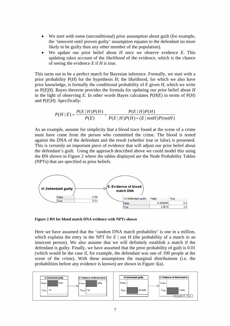
As an example, assume for simplicity that a blood trace found at the scene of a crime must have come from the person who committed the crime. The blood is tested against the DNA of the defendant and the result (whether true or false) is presented. This is certainly an important piece of evidence that will adjust our prior belief about the defendant’s guilt. Using the approach described above we could model this using the BN shown in Figure 2 where the tables displayed are the Node Probability Tables (NPTs) that are specified as prior beliefs.

Figure 2 BN for blood match DNA evidence with NPTs shown

Here we have assumed that the ‘random DNA match probability’ is one in a million, which explains the entry in the NPT for E | not H (the probability of a match in an innocent person). We also assume that we will definitely establish a match if the defendant is guilty. Finally, we have assumed that the prior probability of guilt is 0.01 (which would be the case if, for example, the defendant was one of 100 people at the scene of the crime). With these assumptions the marginal distributions (i.e. the probabilities before any evidence is known) are shown in Figure 3(a).

8

(a) prior marginals (b) blood match evidence true

Figure 3 Running the simple model

If we discover a match then, as shown in Figure 3 (b), when we enter this evidence the revised probability for guilt jumps to 99.99%, i.e. 0.9999 so the probability of innocence is now one in 10,000 (note that, although this is a small probability it is still significantly greater than the random match probability; confusing these two is a classic example of the prosecutor’s fallacy [25]). There are, of course, a number of simplifying assumptions in the model here that we will return to later. To avoid fundamental confusions a number of key points about this approach need to be clarified:

1. The inevitability of subjective probabilities. Ultimately, any use of probability

– even if it is based on frequentist statistics – relies on a range of subjective assumptions. Hence, it is irrational to reject the principle of using subjective probabilities. The objection to using subjective priors may be calmed in many cases by the fact that it may be sufficient to consider a range of probabilities, rather than a single value for a prior. For example, in the real case described in [26] it was shown that, taking both the most pessimistic and most optimistic priors, when the impact of the evidence was considered, the range of the posterior probabilities always comfortably pointed to a conclusive result for the main hypothesis.

2. The value of evidence can be captured by the ‘likelihood ratio’.

It is also worth noting that in some cases there may be no need to consider a prior probability for the ultimate hypothesis. For example, the impact of any single piece of evidence E on the ultimate hypothesis can be determined by considering only the likelihood ratio of E, which is the probability of seeing that evidence if the defendant is guilty divided by the probability of seeing that evidence if the defendant is not guilty. An equivalent form of Bayes Theorem (called the ‘odds’ version of Bayes) tells us that the posterior odds of guilt are the prior odds times the likelihood ratio. So, if the likelihood ratio is bigger than 1 then the evidence increases the probability of guilt (with higher values leading to higher probability of guilt) while if it is less than 1 it decreases the probability of guilt (and the closer it gets to zero the lower the probability of guilt). If the likelihood ratio is equal to or close to 1 then E offers no real value at all since it neither increases nor decreases the probability of guilt. Thus, for example, Evett’s crucial expert testimony in the appeal case of R v Barry George [1] (previously convicted of the murder of the TV presenter Jill Dando) focused on the fact that the forensic gunpowder evidence that had led to the original conviction actually had a likelihood ratio of about 1. This is because both P(E | Guilty) and P(E | not Guilty) were approximately equal to 0.01. Yet only P(E | not Guilty) had been presented at the original trial (a report of this can be found in [4] ).

3. The importance of determining the conditional probabilities in an NPT. When lay people are first introduced to BNs there is a tendency to recoil in horror at the thought of having to understand and/or complete an NPT such as the one for E|H in Figure 2. But, in practice, the very same assumptions that are

9

required for such an NPT are normally made implicitly anyway. The benefit of the NPT is to make the assumptions explicit rather than hidden.

4. The need to leave the Bayesian calculations to a Bayesian calculator. Whereas

Figure 1 models the simplest legal argument (a single hypothesis and a single piece of evidence) we generally wish to use Bayesian networks to model much richer arguments involving multiple pieces of possibly linked evidence. While humans (lawyers, police, jurists etc) must be responsible for determining the prior probabilities (and the causal links) for such arguments, it is simply wrong, as we argued in [25], to assume that humans must also be responsible for understanding and calculating the revised probabilities that result from observing evidence. For example, even if we add just two additional pieces of evidence to get a BN like the one in Figure 4, the calculations necessary for correct Bayesian inference become extremely complex. But, while the Bayesian calculations quickly become impossible to do manually, any Bayesian network tool, such as [2][34] enables us to do these calculations instantly.

Figure 4. Hypothesis and evidence in the case of R v Adams (as discussed in [17])

Despite its elegant simplicity and natural match to intuitive reasoning about evidence, practical legal arguments normally involve multiple pieces of evidence (and other issues) with complex causal dependencies. This is the rationale for the work begun in [33] and that we now extend further by showing that there are unifying underlying concepts which mean we can build relevant BN models, no matter how large, that are still conceptually simple because they are based on a very small number of repeated ‘idioms’ (where an idiom is a generic BN structure). We present these crucial idioms in the next section. 3 The idioms for legal reasoning

10

In the original paper on idioms [50] five were presented to cover a wide range of modelling tasks.

• Cause-consequence idiom (Figure 5)— models the uncertainty of an uncertain causal process with observable consequences. Such a process could be physical or cognitive. This idiom is used to model a causal process in terms of the relationship between its causes (those events or facts that are inputs to the process) and consequences (those events or factors that are outputs of the process). The causal process itself can involve transforming an existing input into a changed version of that input or by taking an input to produce a new output. A causal process can be natural, mechanical or intellectual in nature. The cause-consequence idiom is organised chronologically — the parent nodes (inputs) can normally be said to come before (or at least contemporaneously with) the children nodes (outputs). Likewise, support for any assertion of causal reasoning relies on the premise that manipulation or change in the causes affects the consequences in some observable way.

Figure 5 Cause consequence idiom

• Measurement idiom (Figure 6) — models the uncertainty about the accuracy

of some measurement. We use this idiom to reason about the uncertainty we may have about our own judgements, those of others, or the accuracy of the instruments we use to make measurements. The measurement idiom represents uncertainties we have about the process of observation. By observation we mean the act of determining the true attribute, state or characteristic of some entity. The causal directions here can be interpreted in a straightforward way. The true (actual) value must exist before the observation in order for the act of measurement to take place. Next the measurement instrument interacts (physically, functionally or cognitively) with the entity under evaluation and produces some result. This result can be more or less accurate depending on intervening circumstances and biases.

Figure 6: Measurement Idiom

11

• Definitional — models the formulation of many uncertain variables that together form a functional, taxonomic, or an otherwise deterministic relationship.

• Induction idiom — models the uncertainty related to inductive reasoning based on populations of similar or exchangeable members;

• Reconciliation idiom — models the reconciliation of results from competing measurement or prediction systems.

In this paper we are primarily interested in instances of the cause-consequence, measurement and definitional idioms. 3.1 The evidence idiom We can think of the simple BN in Figure 1 (and its extension to multiple pieces of evidence in Figure 4) as the most basic BN idiom for legal reasoning. This basic idiom, which we call the evidence idiom, is an instantiation of the cause-consequence idiom and has the generic structure shown in Figure 7.

…….

Figure 7 Evidence idiom

We do not distinguish between evidence that supports the prosecution (H true) and evidence that supports the defence (H false) since the BN model handles both types of evidence seamlessly. Hence, this idiom subsumes two of the basic patterns in Hepler at al [33], namely:

1. Corroboration pattern: this is simply the case where there are two pieces of evidence E1 and E2 that both support one side of the argument.

2. Conflict pattern: this is simply the case where there are two pieces of evidence E1 and E2 with one supporting the prosecution and the other supporting the defence.

The evidence idiom has a number of limitations in real cases. The following idioms identify and address these various limitations in turn.

12

3.2 The evidence accuracy idiom Let us return to the example of Figure 2 of evidence in the form of matching DNA from blood found at the scene of the crime. It turns out that the simple model presented made ALL of the following previously unstated assumptions:

• The blood tested really was that found at the scene of the crime • The blood did not become contaminated at any time • The science of DNA is perfect. i.e. there is no possibility of wrongly finding a

match (note, this is very different to the assumption inherent in the random match probability)

• The person presenting the DNA evidence in court does so in a completely truthful and accurate way.

If any of the above is uncertain then the presentation of evidence of blood match DNA being true or false cannot be simply accepted unconditionally. It must necessarily be conditioned on the overall accuracy/reliability of the evidence. In general, the validity of any piece of evidence has uncertainty associated with it, just as there is uncertainty associated with the main hypothesis of guilt. A more appropriate model for this example is therefore the one presented in Figure 8, which is an instantiation of the measurement idiom.

Figure 8 Revised model: Evidence conditioned on its accuracy with NPTs shown

For simplicity we have lumped together all possible sources of inaccuracy into a single node (we shall consider a more complete solution later). Because we have introduced a new variable A into the model the NPT for the node E is more complex. We can think of the original model as being a special case of this model where A was never a doubt (i.e. the accuracy of the evidence was always “true”). So when A is true the NPT for the node E is identical to the NPT in the original model. What is different about the NPT as specified in Figure 8 is the inclusion of our assumptions about the probability of E when A is false. The initial probabilities are shown in Figure 9(a).When evidence of a blood match is presented, Figure 9(b), the probability of guilty increases from the prior 1% to just over 16%. Those who are new to Bayesian reasoning may be surprised that the probability of guilt is so low despite the very low (one in a million) random match probability error.

13

(a) Initial probabilities (b) evidence of blood match presented

Figure 9 Running the model

In fact, the model is working rationally because it is looking for the most likely explanation of the blood match evidence. The prior probability of guilt was 1 in a 100 and this is low compared to the prior probability of inaccurate evidence (1 in 10). So, when only the blood match evidence is presented, the model points to inaccurate evidence as being a more likely explanation for the result. Indeed the probability of inaccurate evidence jumps from 0.1 to nearly 0.85. However, if we determine that the evidence is accurate, as shown in Figure 10(a), the probability of guilt now jumps to 99.99% - the same result as in Figure 3(b) because in this scenario the same assumptions are being made. This is an example of ‘explaining away’ evidence (something we shall return to in Section 3.6).

(a) Blood match evidence is known to be accurate (b) Blood match evidence known to be

inaccurate

Figure 10 Different scenarios of evidence accuracy

If we determine the evidence is inaccurate the result is shown in Figure 10(b). In this case the evidence is worthless and the probability of guilt is unchanged from its prior value of 1 in a 100. By explicitly representing evidence accuracy with a separate variable in the BN it is much easier to see that the prior probabilities of both guilt and evidence accuracy are relevant to computing the probability of guilt given the evidence report (blood match). More generally, this idiom clarifies what inferences should be drawn from a positive test result. This is of practical importance because people (including medical experts)

14

are notoriously poor at calculating the true impact of positive test results [9] [39]. A common error is to ignore the prior probabilities (base-rate neglect), and assume that the probability of the hypothesis (diagnosis) given the evidence is equivalent to the probability of the evidence given the hypothesis (akin to the prosecutor’s fallacy [8]). Use of the BN idiom is likely to reduce this error, by making the problem structure explicit. Indeed a recent set of studies [40] show that base-rate neglect is attenuated when people have an appropriate causal model on which to map the statistics. This supports the use of causal idioms for rational inference. The general idiom to model evidence accuracy is shown in Figure 11. It is an instance of the measurement idiom because we can think of the evidence as simply a measure of (the truth of) the hypothesis. The more accurate the evidence, the closer the evidence value is to the real truth value of the hypothesis.

Figure 11 General idiom to model evidence taking account of its accuracy

To take account of all the individual sources of uncertainty for the DNA blood match example explained at the start of the section we simply apply the idiom repeatedly as shown in Figure 12 (Of course the different accuracy nodes will in general have different prior probabilities).

15

Figure 12 Full BN for DNA blood match evidence accuracy

There are a number of ways in which the evidence accuracy can be tailored. In particular,

1. There is no need to restrict the node accuracy of evidence to being a Boolean (false, true). In general it may be measured on a more refined scale, for example, a ranked scale like {very low, low, medium, high, very high} where very low means “completely inaccurate” and very high means “completely accurate”.

2. In the case of eye witness evidence, it is possible to extend the idiom by

decomposing ‘accuracy’ into three components: competence, objectivity, and veracity as shown in Figure 13.

16

Figure 13 Eye witness evidence accuracy idiom

This is essentially what is proposed in Hepler at al [33], who use the word ‘credibility’ to cover what we call ‘accuracy’, although it should be noted that Hepler et al use an unusual causal structure in which competence influences objectivity, which in turn influences veracity. Our decomposition of accuracy is simply an instance of the definitional idiom. This version of the idiom could also be represented using the object-oriented notation used in [33]; this is shown in Figure 14.

Figure 14 Eye witness accuracy idiom shown using object oriented structuring

3.3 Idioms to deal with the key notions of ‘motive’ and ‘opportunity’ In the examples so far the ultimate hypothesis (defendant is guilty) has been modelled as a node with no parents. As discussed, this fits naturally with the intuitive approach to legal reasoning whereby it is the hypothesis about which we start with an unconditional prior belief before observing evidence to update that belief. But there are two very common types of evidence which, unlike all of the examples seen so far, support hypotheses that are causes, rather than consequences, of guilt. These

17

hypotheses are concerned with ‘opportunity’ and ‘motive’ and they inevitably change the fundamental structure of the underlying causal model. Opportunity: When lawyers refer to ‘opportunity’ for a crime they actually mean a necessary requirement for the defendant’s guilt. By far the most common example of opportunity is “being present at the scene of the crime”. So, for example, if Joe Bloggs is the defendant charged with slashing the throat of Fred Smith at 4 Highlands Gardens on 1 January 2011, then Joe Bloggs had to be present at 4 Highlands Gardens on 1 January 2011 in order to be guilty of the crime. The correct causal BN model to represent this situation (incorporating the evidence accuracy idiom) is shown in Figure 15.

Figure 15 Idiom for incorporating ‘opportunity’ (defendant present at scene of crime)

Note that, just as the hypothesis “defendant is guilty” is unknowable to a jury, the same is true of the opportunity hypothesis. Just like any hypothesis in a trial, its truth value must be determined on the basis of evidence. In this particular example there might be multiple types of evidence for the opportunity hypothesis, each with different levels of accuracy as shown in Figure 16.

Figure 16 Multiple types of evidence for opportunity hypothesis

From a Bayesian inference perspective, the explicit introduction of opportunity into a legal argument means that it is no longer relevant to consider the prior unconditional probability of the ultimate hypothesis (defendant guilty). Although this destroys the

18

original simplified approach it does actually make the overall demands on both the jury and lawyers much clearer as follows:

• The hypothesis requiring an unconditional prior now is that of the opportunity. Unlike the ultimate hypothesis, it is much more likely to be able to base the prior for opportunity on objective information such as the proximity of the defendant’s work/home and the frequency with which the defendant was previously present at the location of the crime scene.

• Determining the NPT for the conditional probability of the ultimate hypothesis given the opportunity (i.e. H2 | H1) also forces the lawyers and jurors to consider rational information such as the total number of people who may have been present at the crime scene.

Motive: There is a widespread acceptance within the police and legal community that a crime normally requires a motive (this covers the notions of ‘intention’ and ‘premeditation’). Although, unlike opportunity, a motive is not a necessary requirement for a crime, the existence of a motive increases the chances of it happening. This means that, as with opportunity, the correct causal BN model to represent motive in a legal argument is shown in Figure 17.

Figure 17 Idiom for incorporating motive

As with opportunity, the introduction of a motive into a legal argument means that it is no longer relevant to consider the prior unconditional probability of the ultimate hypothesis (defendant guilty). But again, this actually makes the overall demands on both the jury and lawyers much clearer as follows:

• Although determining an unconditional prior for motive may be just as hard as determining an unconditional prior for guilt, the argument will in general not be so sensitive to the prior chosen. This is because a motive will generally only be introduced if the lawyer has strong evidence to support it, in which case, irrespective of the prior, its truth value will generally be close to true once the evidence is presented.

• Hence, what really matters is determining the conditional probability of the ultimate hypothesis given the motive. Making this explicit potentially resolves what many believe is one of the most confusing aspects of any trial. Indeed

19

any lawyer who introduces the notion of a motive should be obliged to state what he believes the impact of that motive on guilt to be.

If we wish to include both opportunity and motive into the argument then the appropriate BN idiom is shown in Figure 18

Figure 18 Incorporating both opportunity and motive

This makes the task of defining the NPT for the ultimate hypothesis H a bit harder, since we must consider the probability of guilt conditioned on both opportunity and motive, but again these specific conditional priors are inevitably made implicitly anyway.

Figure 19: A structure to be avoided - conditioning H on multiple motives

What we do need to avoid is conditioning H directly on multiple motives, i.e. having multiple motive parents of H as shown in Figure 19. Instead, if there are multiple motives, we simply model what the lawyers do in practice in such cases: specifically, they consider the accuracy of each motive separately but jointly think in terms of the strength of overall motive. The appropriate model for this is shown in Figure 18 (using the object-oriented notation).

20

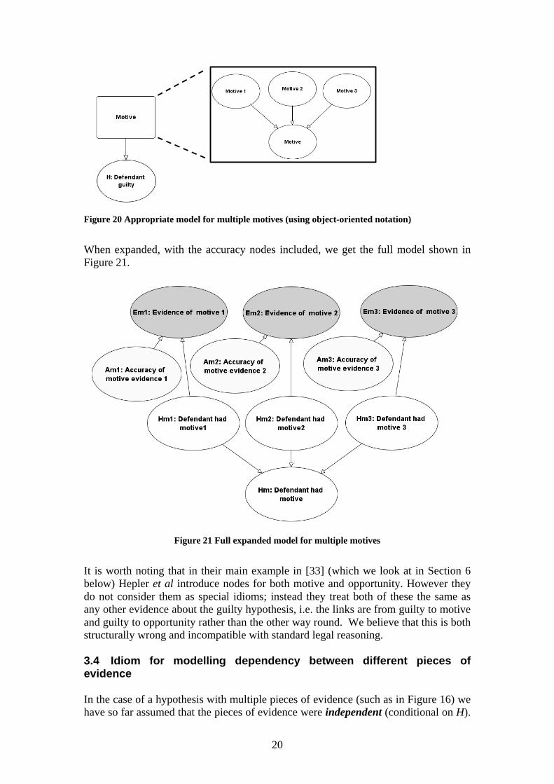
Figure 20 Appropriate model for multiple motives (using object-oriented notation)

When expanded, with the accuracy nodes included, we get the full model shown in Figure 21.

Figure 21 Full expanded model for multiple motives

It is worth noting that in their main example in [33] (which we look at in Section 6 below) Hepler et al introduce nodes for both motive and opportunity. However they do not consider them as special idioms; instead they treat both of these the same as any other evidence about the guilty hypothesis, i.e. the links are from guilty to motive and guilty to opportunity rather than the other way round. We believe that this is both structurally wrong and incompatible with standard legal reasoning. 3.4 Idiom for modelling dependency between different pieces of evidence In the case of a hypothesis with multiple pieces of evidence (such as in Figure 16) we have so far assumed that the pieces of evidence were independent (conditional on H).

21

But in general we cannot make this assumption. Suppose, for example, that the two pieces of evidence for ‘defendant present at scene’ were based on expert analysis of two video cameras placed 20 metres apart. In this case there is clear dependency between the two pieces of evidence: if the expert determines, from the first camera that the defendant is present, there is clearly a much greater chance that the same will be true of the second camera, irrespective of whether the defendant was or was not present. The same is true if the expert determines, from the first camera, that the defendant is not present. This is because of common biases, assumptions, and sources of inaccuracies. The appropriate way to model this would be as shown in Figure 22. This introduces a direct dependency between the two pieces of evidence (it may also be necessary to introduce a ‘common’ accuracy parent node for A1 and A2 if it is assumed that the cameras suffer from common design faults and common failures, but for simplicity we avoid this here).

Figure 22 Introducing dependency between evidence

The associated NPT for E2 would look something like that shown in Figure 23.

Figure 23 NPT for E2 given A2, H1 and E1

Note (from the left hand side of the table) that we are assuming here that if the second camera is inaccurate then there is a 90% probability that E2 will simply ‘copy’ the value of E1 (so, e.g., if E1 is true there is a 90% chance that E2 will be true irrespective of the value of H1). If we assume that the priors for H1, A1 and A2 are all uniform (i.e. 50% true, 50% false) then it is instructive to compare the results between the two models: a) where no direct dependence between E1 and E2 is modelled; and b) where it is. Hence in Figure 24 we show both models in the case where evidence E1 is presented as true. Note the following:

• Both models result in the same (increased) revised belief in H1.

22

• Because of the increased belief in H1, both models lead to an increased probability that E2 will also be presented as true. However, the probability is greater in case (b) (at 82.5%) than in case (a) (at 62.5%).

• Because of the uniform priors the observation of a single piece of evidence has not changed our confidence in the accuracy of the evidence.

a)

b)

Figure 24 Comparing a) no dependence and b) dependence models when E1 is true.

Figure 25 shows the results of E1 and E2 being presented as true in both cases. Although in both cases the probability of H1 being true has increased further, the crucial point to note is that the probability is higher in the case where E1 and E2 are independent. This is because, of course, the evidence of E2 in case (b) is no longer as convincing as in case (a).

23

a)

b)

Figure 25 Comparing a) no dependence and b) dependence models when both E1 and E2 are true. One apparently curious outcome in Figure 25(b) is that the probability of A2 being true has dropped below 50%. But again the BN calculation is perfectly rational; the reason for the drop is the prior belief that, when A2 is false, there is a 90% probability that the value of E2 will be the same as E1 (i.e. when false it is very likely to simply ‘copy’ E2). So when we actually observe that the value of E2 is the same as E1 the BN calculates that this is more likely due to A2 being false than to H1 being true. The benefits of making explicit the direct dependence between evidence are enormous. For example, in the case of the Levi Bellfield trial described in [25] the prosecution presented various pieces of directly dependent evidence in such a way as to lead the jury to believe that they were independent, hence drastically overstating the impact on the hypothesis being true. In fact, a simple model of the evidence based on the structure above showed that, once the first piece of evidence was presented, the subsequent evidence was almost useless, in the sense that it provided almost no further shift in the hypothesis probability. An important empirical question is the extent to which laypeople (and legal professionals) are able to discount the value of dependent evidence. Research in [58] suggests that people sometimes ‘double-count’ redundant evidence. This would lead to erroneous judgments, so it is vital to explore the generality of this error, and whether it can be alleviated by use of the BN framework proposed in this paper.

24

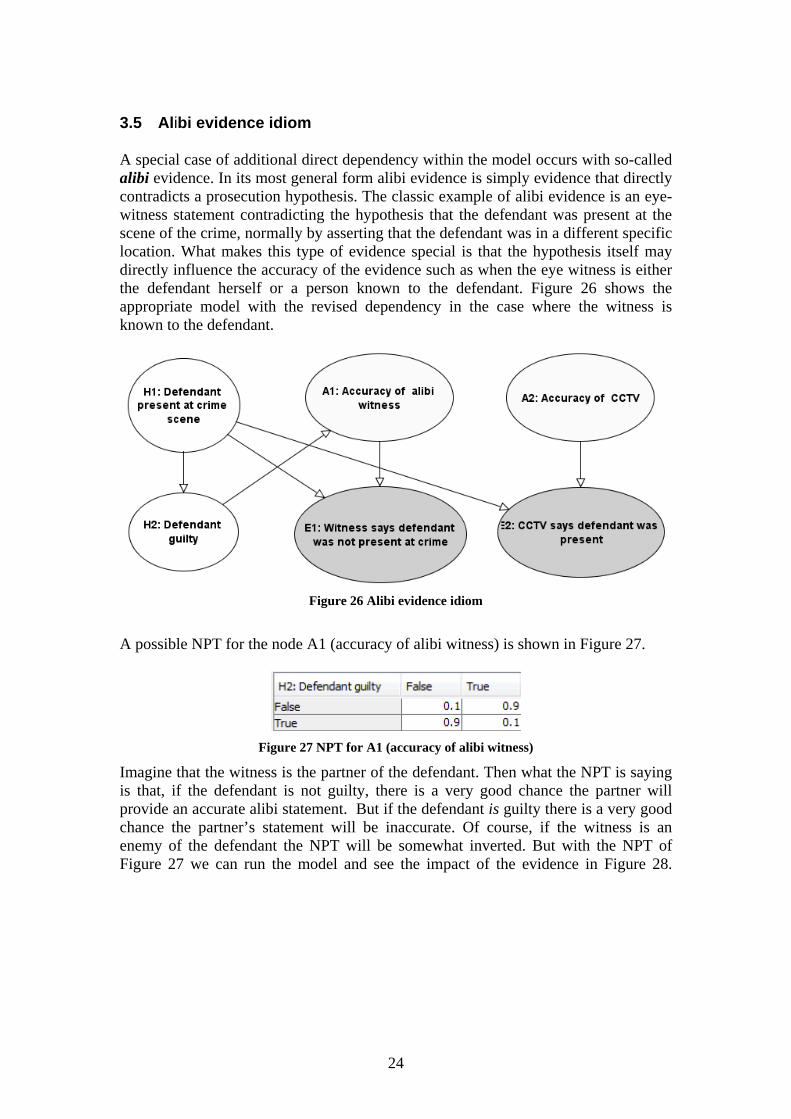
3.5 Alibi evidence idiom A special case of additional direct dependency within the model occurs with so-called alibi evidence. In its most general form alibi evidence is simply evidence that directly contradicts a prosecution hypothesis. The classic example of alibi evidence is an eye-witness statement contradicting the hypothesis that the defendant was present at the scene of the crime, normally by asserting that the defendant was in a different specific location. What makes this type of evidence special is that the hypothesis itself may directly influence the accuracy of the evidence such as when the eye witness is either the defendant herself or a person known to the defendant. Figure 26 shows the appropriate model with the revised dependency in the case where the witness is known to the defendant.

Figure 26 Alibi evidence idiom

A possible NPT for the node A1 (accuracy of alibi witness) is shown in Figure 27.

Figure 27 NPT for A1 (accuracy of alibi witness)

Imagine that the witness is the partner of the defendant. Then what the NPT is saying is that, if the defendant is not guilty, there is a very good chance the partner will provide an accurate alibi statement. But if the defendant is guilty there is a very good chance the partner’s statement will be inaccurate. Of course, if the witness is an enemy of the defendant the NPT will be somewhat inverted. But with the NPT of Figure 27 we can run the model and see the impact of the evidence in Figure 28.

25

a) Prior probabilities

b) Alibi evidence only

c) CCTV evidence only

d) Conflicting evidence (both CCTV and alibi)

Figure 28 Impact of alibi evidence

26

The model provides some very powerful analysis, notably in the case of conflicting evidence (i.e. where one piece of evidence supports the prosecution hypothesis and one piece supports the defence hypothesis). The most interesting points to note are:

• When presented on their own ((b) and (c) respectively), both pieces of evidence lead to an increase in belief in their respective hypotheses. Hence, the alibi evidence leads to an increased belief in the defence hypothesis (not guilty) and the CCTV evidence leads to an increased belief in the prosecution hypothesis (guilty). Obviously the latter is much stronger than the former because of the relative priors for accuracy, but nevertheless on their own they both provide support for their respective lawyers’ arguments.

• When both pieces of evidence are presented (d) we obviously have a case of conflicting evidence. If the pieces of evidence were genuinely independent the net effect would be to decrease the impact of both pieces of evidence on their respective hypotheses compared to the single evidence case. However, here because the alibi evidence is dependent on H2, the result is that the conflicting evidence actually strengthens the prosecution case even more than if the CCTV evidence was presented on its own. Specifically, because of the prior accuracy of the CCTV evidence, when this is presented together with the alibi evidence it leads us to doubt the accuracy of the latter (we tend to believe the witness is lying) and hence, by backward inference, to increase the probability of guilt.

This analysis of alibi evidence has direct relevance to legal cases. Indeed two key issues that arise when an alibi defence is presented in court are (1) whether or not the alibi provider is lying, and (2) what inferences should be drawn if one believes that they are lying. In cases where an alibi defence is undermined, judges are required to give special instructions alerting the jury to the potential dangers of drawing an inference of guilt. In particular, the judge is supposed to tell the jury that they must be sure that the alibi provider has lied, and sure that the lie does not admit of an innocent explanation [15]. We maintain that the correct way to model alibi evidence, and to assess what inferences can be legitimately drawn from faulty alibis, is via the BN framework. Moreover, recent empirical studies show that ordinary people draw inferences in line with the proposed alibi idiom [41][42]. For example, when given the scenario discussed above, judgments of the suspect’s guilt are higher when both alibi evidence and disconfirming CCTV evidence are presented, then when CCTV evidence alone is presented. This holds true even though the alibi evidence by itself reduces guilt judgments. This pattern of inference is naturally explained by the supposition that the suspect is more likely to lie if he is guilty rather than innocent. 3.6 Explaining away idiom One of the most powerful features of BN reasoning is the concept of ‘explaining away’. An example of explaining away was seen in the evidence accuracy idiom in Figure 10. The node E (evidence of blood match) has two parents H (defendant guilty) and A (accuracy of evidence) either of which can be considered as being possible ‘causes’ of E. Specifically, H being true can cause E to be true, and A being false can cause E to be true. When we know that the blood match evidence has been presented (i.e. E is true) then, as shown in Figure 10b, the probability of both potential ‘causes’ increases (the probability of H being true increases and the probability of A being false increases). Of the two possible causes the model favours A being false as

27

the most likely explanation for E being true. However, if we know for sure that A is true (i.e. the evidence is accurate) then, as shown in Figure 10c, we have explained away the ‘cause’ of E being true - it is now almost certain to be H being true. Hepler et al [33] consider ‘explaining away’ as an explicit idiom 5.4 as shown in Figure 29.

Figure 29 Hepler at al's explaining away idiom

Hepler’s et al’s example of their explaining way idiom also turns out to be a special case of the evidence accuracy idiom. In their example the event is ‘defendant confesses to the crime’, and the causes are 1) defendant guilty and 2) defendant coerced by interrogating official. Using our terminology the ‘event’ is clearly a piece of evidence and cause 2 characterises the accuracy of the evidence. However, it turns out that traditional ‘explaining away’ does not work in a very important class of situations that are especially relevant for legal reasoning. These are the situations where the two causes are mutually exclusive, i.e. if one of them is true then the other must be false. Suppose, for example, that we have evidence E that blood found on the defendant’s shirt matches the victim’s blood. Since there is a small chance (let us assume 1%) that the defendant’s blood is the same type as the victim’s, there are two possible causes of this:

• Cause 1: the blood on the shirt is from the victim • Cause 2: the blood on the shirt is the defendant’s own blood

In this case only one of the causes can be true. But the standard approach to BN modelling will not produce the correct reasoning in this example. To see why, let us consider how we should define the NPT for E. Figure 30 seems reasonable (assuming no errors are made on blood matching). Columns 1 and 3 are uncontroversial while column 2 captures our assumption about the probability both victim and defendant have same blood type. The interesting case is column 4 when both causes are true. It seems reasonable that the probability E being true in this case is 1 (since this is the case when just cause 1 is true).

Figure 30 Possible NPT for E (Blood on shirt matches victim)

28

But, if we run this model (using uniform priors for cause 1 and cause 2) then although backward inference seems correct when we observe E as true (Figure 31(a)) it clearly fails to produce the ‘correct’ result when we know cause 2 is true ((Figure 31(b)).

(a) Backward inference seems to work OK (b) Cause 1 should be False in this scenario

Figure 31 Running the model

There is an even more fundamental problem with the model. Irrespective of E, if either cause is true then the other should be false. The model does not produce this result even if we attempt to introduce a dependency between the two causes. The solution is to apply the definitional idiom to specify those states in our model that are, by definition, mutually exclusive. At first glance it seems the best way to do this is to replace two separate cause nodes with a single cause node that has mutually exclusive states. Unfortunately, this approach is of little help in most legal reasoning situations because we will generally want to consider distinct parent and child nodes of the different causes, each representing distinct and separate causal pathways in the legal argument. For example, cause 2 may itself be caused by the defendant having cut himself in an accident; since cause 1 is not conditionally dependent on this event it makes no sense to consider the proposition “blood on shirt belongs to victim because the defendant cut himself in an accident”. We cannot incorporate these separate pathways into the model in any reasonable way if cause 2 is not a separate node from cause 1. The pragmatic solution using the definitional idiom that works in this case is to introduce a new node that operates as a constraint on the cause 1 and cause 2 nodes as shown in Figure 32.

Figure 32 Explaining away idiom with constraint node and its NPT

29

As shown in the figure the NPT of this new constraint node has three states: one for each causal pathway plus one for “impossible”. The impossible state can only be true when either a) both causes 1 and 2 are false or b) both causes 1 and 2 are true. Given our assumption that the causes are mutually exclusive these conjoint events are by definition impossible, hence the choice of the third state label. To ensure that impossibility is excluded in the model operationally we enter what is called “soft evidence” on the constraint node. This is a standard BN technique (available in most BN tools) whereby instead of setting a single state of a node to be true (as in entering the normal – hard - evidence) we can set a number of states to be true with different probabilities. In this case the soft evidence we set for the constraint node is that the states “cause 1” and “cause 2” each have 50% probability while the state “impossible” has 0% probability. The model then works exactly as expected. A complete example, which also shows how we can extend the use of the idiom to accommodate other types of deterministic constraints in the possible combinations of evidence/hypotheses, is shown in Figure 33.

Figure 33 Full example of mutually exclusive causes

In this example, if we assume uniform priors for the nodes without parents, then once we set the evidence of the blood match as True, and the soft evidence on the Constraint node as describe above, we get the result shown in Figure 34.

30

Figure 34 Evidence of blood match set to true

In the absence of other evidence this clearly points to cause 1 (blood on the shirt is from the victim) as being most likely and so strongly favours the guilty hypothesis. However, when we enter the evidence a) victim and defendant have same blood type and b) defendant has recent scar then we get the very different result shown in Figure 35. This clearly points to cause 2 as being the most likely.

Figure 35 New defence evidence is entered

So, in summary, the key points about the above special ‘explaining away’ idiom are:

31

• It should be used when there are two or more mutually exclusive causes of E, each with separate causal pathways

• The mutual exclusivity acts as a constraint on the state-space of the model and can be modelled as a constraint

• When running the model soft evidence must be entered for the constraint node to ensure that impossible states cannot be realised in the model.

Using constraint nodes in this way also has the benefit of a) revealing assumptions about the state space that would be otherwise tacit or implicit and b) helping to keep causal pathways cleaner at a semantic level. 4 Putting it all together: 4.1 Example 1: The impact of discredited evidence Before showing a comprehensive example of the use of the method we apply it to show how it naturally handles the distinction between different types of discredited evidence (the subject of discredited evidence was discussed at length in [41] and we shall return to it again later in the context of the order in which evidence is presented). Consider the following example from [43]:

.. a suspect is accused of house burglary, and a witness testifies that the suspect was loitering in the area a few days before the crime (statement A). This same witness also testifies that she saw the suspect near the crime scene on the night of the crime (statement B). What happens if it is subsequently discovered that the witness has fabricated statement B. For example, perhaps there is strong evidence that she was out of town on the night in question, but fabricated her statement because she dislikes the suspect? Clearly one should disregard statement B – it no longer provides valid evidence against the suspect. But what about statement A? Should this also be disregarded?

This example is contrasted with the example of two completely independent witnesses providing evidence A and B respectively. Our proposed BN structuring method easily handles the distinction between the two cases. First, let us assume that the witnesses are independent. Then the appropriate model is shown in Figure 36.

32

Figure 36 Independent witness evidence

Note that the model makes a number of important clarifications. In particular, the two different pieces of evidence A and B are not direct evidence of the hypothesis “defendant guilty”. Rather, they are respectively evidence to support motive (that is what the previous loitering suggests) and opportunity (present at the crime scene). If the two pieces of evidence are presented from the same witness then the correct model is the one shown in Figure 37, where we have introduced a direct dependency between the accuracy of the two pieces of evidence. In this case the direction of the link does not matter to the overall argument.

Figure 37 Same witness evidence

Using uniform priors for the parentless nodes and uncontroversial NPTs for the other nodes, when we run the two models we get the results shown in Table 1

33

Table 1 Results of running both models

Independent witnesses Same witness probability Guilty probability Guilty Prior state 50% 50% Evidence A presented 55% 55% Evidence B presented 75% 75% Accuracy of B false 55% 51%

So as we enter evidence A and B in turn we get the same impact on probability of guilty. However, when we discredit evidence B there is a marked difference between the models in the posterior probability of guilty. Figure 38 shows the full model distributions in this final case. The key difference is that evidence B being inaccurate propagates back in (b) to a low belief in the accuracy of evidence A.

(a) Independent witnesses (b) Same witness

Figure 38 Models compared

4.2 Vole Example In [41] there is the following case based on Agatha Christie’s play “Witness for the prosecution”.

Leonard Vole is charged with murdering a rich elderly lady, Miss French. He had befriended her, and visited her regularly at her home, including the night of her death. Miss French had recently changed her will, leaving Vole all her money. She died from a blow to the back of the head. There were various pieces of incriminating evidence: Vole was poor and looking for work; he had visited a travel agent to enquire about luxury cruises soon after Miss French had changed her will; the maid claimed that Vole was with Miss French shortly before she was killed; the murderer did not force entry into the house; Vole had blood stains on his cuffs that matched Miss French’s blood type. As befits a good crime story, there were also several pieces of exonerating evidence: the maid admitted that she disliked Vole; the maid was previously the sole benefactor in Miss French’s will; Vole’s blood type was the same as Miss French’s, and thus also matched the blood found on his cuffs; Vole claimed that he had cut his wrist slicing ham; Vole had a scar on his wrist to back this claim. There was one other critical piece of defence evidence: Vole’s wife, Romaine, was to testify that Vole had returned home at 9.30pm. This would place him far away

34

from the crime scene at the time of Miss French’s death. However, during the trial Romaine was called as a witness for the prosecution. Dramatically, she changed her story and testified that Vole had returned home at 10.10pm, with blood on his cuffs, and had proclaimed: ‘I’ve killed her’. Just as the case looked hopeless for Vole, a mystery woman supplied the defence lawyer with a bundle of letters. Allegedly these were written by Romaine to her overseas lover (who was a communist!). In one letter she planned to fabricate her testimony in order to incriminate Vole, and rejoin her lover. This new evidence had a powerful impact on the judge and jury. The key witness for the prosecution was discredited, and Vole was acquitted. After the court case, Romaine revealed to the defence lawyer that she had forged the letters herself. There was no lover overseas. She reasoned that the jury would have dismissed a simple alibi from a devoted wife; instead, they could be swung by the striking discredit of the prosecution’s key witness.

To model the case Lagnado [41] presents the causal model shown in Figure 39.

Figure 39 Model from [41]

What we will now do is build the model from scratch using only the idioms introduced. In doing so we demonstrate the effectiveness and simplicity of our proposed method (which provides a number of clarifications and improvements over the original model). Most importantly we are able to run the model to demonstrate the changes in posterior guilt that result from presenting evidence in the order discussed in the example. Step 1: Identify the key prosecution hypotheses (including opportunity and motive)

• The ultimate hypothesis “H0: Vole guilty” • Opportunity: “Vole present” • Motive: There are actually two possible motives “Vole poor” and “Vole in

will” Step 2: Consider what evidence is available for each of the above and what is the accuracy of the evidence:

35

Evidence for H0. There is no direct evidence at all for H0 since no witness testifies to observing the murder. But what we have is evidence for are two hypotheses that depend on H0:

• H1: Vole admits guilt to Romaine • H2: Blood on Vole’s shirt is from French

Of course, neither of these hypotheses is guaranteed to be true if H0 is true, but this uncertainty is modelled in the respective NPTs. The (prosecution) evidence to support H1 is the witness statement by Romaine. Note that Romaine’s evidence of Vole’s guilt makes her evidence of “Vole present” redundant (so there is no need for the link from “Vole present” to Romaine’s testimony in the original model). The issue of accuracy of evidence is especially important for Romaine’s evidence. Because of her relationship with Vole the H1 hypothesis influences her accuracy. Evidence to support H2 is that the blood matches French’s The evidence to support the opportunity “Vole present” is a witness statement from the Maid.

Step 3: Consider what defence evidence is available to challenge the above hypotheses.

The evidence to challenge H1 is the (eventual) presentation of the love letters and the introduction of a new (defence) hypothesis “H4: Romaine has lover”. The evidence to challenge the opportunity “Vole present” is a) to explicitly challenge the accuracy of the Maid’s evidence and b) Vole’s own alibi evidence. The evidence to challenge H2 is that the blood matches Vole’s (i.e. Vole and French have the same blood type). Additionally, the defence provides an additional hypothesis “H3: Blood on Vole is from previous cut” that depends on H2.

Finally, for simplicity we shall assume that some evidence (such as the blood match evidence) is perfectly accurate and that the motives are stated (and accepted) without evidence. From this analysis we get the BN shown in Figure 40.

36

Figure 40 Revised Vole model

Note how the model is made up only from the idioms we have introduced (the blood match component is exactly the special “explaining away” idiom example described in Section 3.5). With the exception of the node H5 (Romaine has lover) the priors for all parentless nodes are uniform. The node H5 has prior set to True = 10%. What matters when we run the model is not so much whether the probabilities are realistic but rather the way the model responds to evidence. Hence, Figure 41 shows the effect (on probability of guilt) of the evidence as it is presented sequentially, starting with the prosecution evidence.

Sequential Presentation of Evidence H0 Vole guilty Probability Prosecution evidence presented

1. Prior (no observations) 33.2% 2. Motive evidence added (M1 and M2 = true) 35.8 3. Maid testifies Vole was present = true 52.6% 4. E3 blood matches French evidence = true 86.5% 5. Romaine testifies Vole admitted guilt = true 96.6%

Defence evidence presented

6. Vole testifies he was not present = true 96.9% 7. Maid evidence accuracy = false 91.3% 8. E4 Blood matches Vole = true 64.4% 9. E5 Vole shows scar = true 40.4% 10. Letters as evidence - true 14.9%

Figure 41 Effect on probability of guilt of evidence presented sequentially

The key points to note here are that:

37

• The really ‘big jump’ in belief in guilt comes from the introduction of the blood match evidence (at this point it jumps from 52.6% to 86.5%). However, if Romaine’s evidence had been presented before the blood match evidence that jump would have been almost as great (52.6% to 81%).

• Once all the prosecution evidence is presented (and bear in mind that at this point the defence evidence is set to the prior values) the probability of guilt seems overwhelming (96.6%)

• If, as shown, the first piece of defence evidence is Vole’s own testimony that he was not present, then the impact on guilt is negligible. This confirms that, especially when seen against stronger conflicting evidence, an alibi that is not ‘independent’ is very weak. Although the model does not incorporate the intended (but never delivered) alibi statement by Romaine, it is easy to see that there would have been a similarly negligible effect, i.e. Romaine’s suspicions about the value of her evidence are borne out by the model.

• The first big drop in probability of guilt comes with the introduction of the blood match evidence.

• However, when all but the last piece of defence evidence is presented the probability of Vole’s guilt is still 40.4% - higher than the initial probability. Only when the final evidence – Romaine’s letters – are presented do we get the dramatic drop to 14.9%. Since this is considerably less than the prior (33.2%) this should certainly lead to a not guilty verdict if the jury were acting as rational Bayesians.

It is also worth noting the way the immediate impact of different pieces of evidence is very much determined by the order in which the evidence is presented. To emphasize this point Figure 42 presents a sensitivity analysis, in the form of a Tornado chart, of the impact of each possible piece of evidence individually on the probability of guilt. From this graph we can see, for example, that if all other observations are left in their prior state, the Vole blood match evidence has the largest impact on Vole guilty; when it is set to true the probability of guilt drops to just over 10% and when it is set to false the probability of guilt jumps to nearly 90%. The French blood match evidence has a very similar impact. At the other extreme the individual impact of the Romaine letters is almost negligible. This is because this piece of evidence only becomes important when the particular combination of other evidence has already been presented.

38

Figure 42 Sensitivity analysis on guilty hypothesis

4.3 Sacco and Vanzetti case In [33] Hepler et al apply their BN framework to the Sacco and Vanzetti case as described in [38]. We apply our idioms to the case and believe that the resulting structure is more elegant and accurate. We focus on the same part of the case covered in [33] Figure 4 (with further breakdown in Figures 9 and 10), namely the case for Sacco being at the scene of the crime. Our model is presented in Figure 43.

39

Figure 43 BN for Sacco and Vanzetti case

We have used the same shading conventions as before (evidence nodes in dark shading, accuracy nodes light shading, and hypothesis nodes unshaded), but this time we have distinguished prosecution and defence hypotheses and evidence nodes by making the former bold. The ultimate hypothesis here is “Sacco at scene”. The whole model is built only from instances of the evidence accuracy idiom. The improvements/corrections over the model in [33] are:

• Some of Wade’s testimony is directly about the “Sacco at scene” hypothesis and some is about “Man similar to Sacco at scene” ([33] wrongly assumes only the latter). Figures 9 and 10 of [33] are wrong structurally with respect to Wade.

• The handling of the Frantello testimony in [33] is structurally wrong. • The model in Fig 4 of [33] did not include the crucial Pelser component

In wider discussions of the case Figure 7 of [33] introduces an explicit node called ‘motive’ and an ‘opportunity’ node (“At Scene”) as we already mentioned in Section 3.3. But Hepler et al treat both of these the same as any other evidence about the guilty hypothesis, i.e. the links are from guilty to motive and guilty to opportunity rather than the other way round. 5 The importance of order of evidence presentation Although the particular order of evidence presentation clearly affects the scale of immediate impact that piece of evidence has on the probability of guilt, ultimately the order should be irrelevant to a rational Bayesian once all the evidence is presented.

40

So, for example, in the Vole BN, no matter what order we enter the 10 pieces of evidence the final probability of guilt will always end up as exactly 14.9% given the same priors. Yet, empirical work in [41] and [43] has demonstrated that sometimes people arrive at different posterior probabilities of guilt when evidence is presented in a different order ([41] refers to this as non-normative reasoning). Does this mean that the subjects in these studies were simply not behaving as rational Bayesians? It turns out that it probably does not mean this and that in practice there are important ramifications of the order in which the evidence is presented. It turns out that our modelling method sheds great insight into this apparent paradox. In the empirical studies in [43] the following problem was considered:

Two pieces of evidence A and B about the guilty hypothesis are presented in order, but one piece of evidence is subsequently discredited.

Using the terminology of [43] there are a number of variations we can consider for this problem

• whether or not A and B are related (such as from the same witness) or unrelated.

• whether or not the discrediting information is presented early (meaning after A but before B) or late (meaning after B).

• whether or not A and B are conflicting evidence (meaning that one supports the prosecution hypothesis of guilty and one supports the defence hypothesis of not guilty) or whether both support one side.

The first empirical study in [43] compared the case of related and unrelated evidence assuming late discredit and non-conflicting evidence. Based on the discussion above the appropriate BN models for these two cases seem to be the ones shown in Figure 44

(a) unrelated evidence (b) related evidence

Figure 44 BNs for unrelated and related evidence case

To see what the ‘normative’ judgements should be we simply run the models with the evidence presented in order. We are assuming uniform priors for each node without parents, while the NPTs for the evidence nodes are all the same as shown in Figure 45(a). The NPT for Accuracy of B in the related evidence model is shown in Figure 45(b).

41

(a) NPT for Evidence A (b) NPT for Accuracy B

Figure 45 NPTs

Running the models gives the results in Table 2. Table 2 Results of running both models

Unrelated Model Related Model probability Guilty probability Guilty Prior state 50% 50% Evidence A presented 74% 74% Evidence B presented 89% 82% Accuracy of B false 74% 54%

Whereas the subjects in the empirical study concurred with the results for the related model (i.e. they correctly reasoned backward that the accuracy of A was likely to be very poor given that B was discredited) the results for the unrelated model did not concur. Specifically, instead of returning to the same probability of guilty as after evidence A was entered, they returned a lower probability. But was this really a case of non-normative reasoning? In fact, it can be argued that the subjects were assuming a different causal model, namely the one shown in Figure 46.

Figure 46 Alternative model for 'unrelated evidence'

In this model the independence of the accuracy of the evidence is conditional on the notion of what we have referred to as ‘lawyer bias’. The job of lawyers is to win the case, and in pursuit of this aim they will attempt to find and bolster whatever evidence is available. If the lawyer is short of strong evidence she is more likely to push weaker (i.e. less accurate evidence). So even if evidence A and B are presented by totally independent witnesses the fact that this evidence is presented at all may be due to the bias of the lawyer.

42

Indeed, when we run this model we get the results shown in Table 3. Table 3 Running the 'bias' model

Bias Model probability Guilty Prior state 50% Evidence A presented 74% Evidence B presented 84% Accuracy of B false 58%

These results concur perfectly with the subjects in the ‘unrelated’ case. This suggests that the subjects were using something like the bias model. It appears that subjects may genuinely start by assuming the model in Figure 44(a), but then switch to the bias model once the discrediting information is provided. After all, the fact that the defence presented discredited information surely suggests some notion of bias in the case. This possibility is certainly supported by the empirical results for the case of early discredit. In this case (when evidence A is discredited immediately after it is presented) the subjects provide the normative results for both the unrelated and related models. So, in the unrelated case they are using the model in Figure 44(a) and not the bias model. This re-interpretation of the findings in [43] is being investigated with further empirical studies. Whereas [43] assumed that the order in which evidence is presented influenced whether or not subjects reasoned normatively, we now believe that the explanation is that the order influences which of different causal models is the most appropriate. Subjects reason normatively but based on alternative models given different order of evidence. From a BN perspective this is, of course, challenging since we had assumed that a single fixed BN could provide an accurate model of the whole legal argument (in the sense that it incorporates all of the relevant prosecution and defence hypotheses and claims) and hence, ultimately the order in which the evidence is presented should not matter to a rational Bayesian. But we made it clear at the beginning that we already were making a major assumption: that there was a single ultimate hypothesis. So we already recognised that with different ultimate hypotheses there will be a need to consider different causal models. The possibility that the prosecution has ‘framed’ the defendant (and hence that apparently unrelated evidence must be seen as conditionally dependent) is just one example of an alternative ultimate hypothesis. This also applies to the Vole case. Although we explicitly modelled the hypothesis that Romaine had a lover, this hypothesis would not have been considered relevant initially. The final empirical study in [43] considered the difference between conflicting and non-conflicting evidence. In the former case it is inevitable that any relationship between the evidence must be extremely weak since one piece of evidence is presented by the defence and the other by the prosecution. In the BN this is modeled by changing the NPT for the node “Accuracy of B”. So, although we can still consider the separate related and unrelated models, the overall results when running the models are similar, namely that discrediting one piece of evidence should not lead to any discrediting of the other. In this case the subjects in the study concurred with the

43

model results. So, not only were they acting rationally, but they also had no need to consider an alternative model since in this case the notion of bias was clearly irrelevant. 6 Roadmap and Conclusions In this paper we have outlined a general framework for modelling legal arguments. The framework is based on Bayesian networks, but introduces a small set of causal idioms tailored to the legal domain that can be reused and combined. This idiom-based approach allows us to model large bodies of interrelated evidence, and capture inference patterns that recur in many legal contexts. The use of small-scale causal idioms fits well with the capabilities and constraints of human cognition, and thus provides a practical method for the analysis of legal cases. The proposed framework serves several complementary functions:

• To provide a normative model for representing and drawing inferences from complex evidence, thus supporting the task of making rational inferences in legal contexts.

• To suggest plausible cognitive models (e.g., representations and inference mechanisms) that explain how people manage to organize and interpret legal evidence.

• To act as a standard by which to evaluate non-expert reasoning (e.g., by jurors); where people depart from the rational model the BN approach provides methods and tools to improve judgments (especially with complex bodies of evidence).

The potential for the BN framework to illuminate the psychology of juror reasoning is relatively unexplored, but empirical findings thus far are encouraging. Research suggests that people naturally use causal models to organize and understand legal evidence [52][53] and can draw rational inferences in simple cases [41][42]. However, there are also apparent anomalies, such as the over-generalization of discrediting evidence and order effects [43]. In this paper we have argued that these anomalies admit of rational explanation, especially when it is acknowledged that people can construct different causal models according to the order in which information is received. These issues are being explored in ongoing empirical studies. In addition, the BN framework, together with the causal idiom approach, suggests numerous fresh avenues for empirical research. We have highlighted some of these throughout the paper; they include the explicit modelling of evidence accuracy, incorporating evidence of motive and opportunity, the inferences drawn from dependent evidence, the interpretation of alibi evidence, the ‘explaining away’ of competing causes, and effects of order of presentation. Many of these questions would not have been formulated without the introduction of a general framework for evidential reasoning. We are now in a position to systematically test how people reason in such contexts, and establish whether they conform to the prescripts of the BN models.

44

Irrespective of how these studies turn out, we believe that it is crucial to build a general inferential framework that allows us to understand and conduct legal argumentation. The proposed BN framework might prove a powerful guide to the representations and inferences that people actually use, but where people depart from this rational model, it will also afford a means for correcting these departures. 7 Acknowledgements This work has benefited from the input of a number of colleagues and experts. We are especially indebted to William Marsh. 8 References [1] (2007). R. v. George, EWCA Crim 2722. [2] Agena Ltd (2010). AgenaRisk, http://www.agenarisk.com. [3] Aitken, C.G.G. and Taroni, F., Statistics and the evaluation of evidence (2nd Edition).

2004 John Wiley & Sons, Ltd. [4] Aitken, C. (2008). Interpreting the Value of Evidence. Royal Statistical Society, 9

Sept 2008. http://www.rss.org.uk/PDF/Colin%20Aitken%20-%209%20Sept%2008.pdf

[5] Aitken, C. G. G., et al. (1995). Bayesian belief networks with an application in specific case analysis. Computational Learning and Probabilistic Reasoning. A. Gammerman, John Wiley and Sons Ltd.

[6] Allen, R. J. and Miller, J. S. (1993). "The Common Law Theory of Experts: Deference or Education?" Northwestern Law Review 87: 1131-1147.

[7] Anderson, T., Schum, D. A. and Twining, W. (2005). Analysis of Evidence, Cambridge University Press.

[8] Balding, D.J. and Donnelly, P., Prosecutor's fallacy and DNA evidence, in Criminal Law Review, 711-722. 1994.

[9] Casscells, W., Schoenberger, A., and Graboys, T.B., Interpretation by physicians of clinical laboratory results. New England Journal of Medicine, 1978. 299 p. 999-1001.

[10] Chase, W. G., & Simon, H. A. (1973). Perception in chess. Cognitive Psychology, 4, 55-81

[11] Cosmides, L. and Tooby, J. (1996). "Are humans good intuitive statisticians after all? Rethinking some conclusions from the literature on judgment under uncertainty." Cognition 58 1-73

[12] Cowan, N. (2001) The magical number 4 in short-term memory: a reconsideration of mental storage capacity. Behavorial & Brain Sciences. 24, 87–185.

[13] Cowell, R. G. (2003). "Finex: a Probabilistic Expert System for forensic identification." Forensic Science International 134(2): 196-206.

[14] Cowell, R., Lauritzen, S. and Mortera, J. (2006). "Identification and separation of DNA mixtures using peak area information." Forensic Science International 166(1): 28-34.

[15] Crown Court Benchbook, Judicial Studies Board, 2010. [16] Dawid, A. P. and Evett, I. W. (1997). "Using a graphical model to assist the

evaluation of. complicated patterns of evidence." Journal of Forensic Sciences 42: 226-231.

[17] Dawid, A. P. (2002). Bayes’s theorem and weighing evidence by juries. In Bayes’s

45

Theorem: Proceedings of the British Academy. R. Swinburne. Oxford, Oxford University Press. 113: 71-90.

[18] Dawid, P., Statistics on Trial. Significance, 2005. 2(1): p. 6-8. 10.1111/j.1740-9713.2005.00075.x

[19] Edwards, W. (1991). "Influence Diagrams, Bayesian Imperialism, and the Collins case: an appeal to reason." Cardozo Law Review 13: 1025-1079.

[20] Ericsson, K. & Kintsch, W. (1995). Long-term working memory. Psychological Review 102: 211–245.

[21] Ericsson, K., Charness, N., Feltovich, P., & Hoffman, R. (2006). Cambridge Handbook of Expertise and Expert Performance. Cambridge, UK: Cambridge University Press.

[22] Evett, I. W. (1995). "Avoiding the transposed conditional." Science and Justice 35(3): 127-131

[23] Evett, I. W. and Weir, B. S. (1998). Interpreting DNA evidence : statistical genetics for forensic scientists, Sinauer Associates.

[24] Faigman, D.L. and Baglioni, A.J., Bayes' theorem in the trial process. Law and Human Behavior, 1988. 12(1): p. 1-17. http://dx.doi.org/10.1007/BF01064271

[25] Fenton, N. E. and M. Neil (2010). "Avoiding Legal Fallacies in Practice Using Bayesian Networks." Australian Journal of Legal Philosophy submitted.

[26] Fenton, N. and M. Neil (2010). "Comparing risks of alternative medical diagnosis using Bayesian arguments." Journal of Biomedical Informatics 43: 485-495.

[27] Fienberg, S. E. and M. J. Schervish (1986). "Relevance of Bayesian Inference for the Presentation of Statistical Evidence and for Legal Decisionmaking, The Symposium." Boston University Law Review 66: 771-798.

[28] Finkelstein, M. O. and Levin, B. A. (2001). Statistics for Lawyers, Springer. [29] Gilovich, T., Griffin, D., and Kahneman, D., Heuristics and Biases: The Psychology

of Intuitive Judgment. . 2002, Cambridge: Cambridge University Press. [30] Gobet, F., Lane, P., Croker, S., Cheng, P., Jones, G., Oliver, I. & Pine, J.

(2001). Chunking mechanisms in human learning. Trends in Cognitive Science, 5, 236-243.

[31] Good, P. I. (2001). Applying Statistics in the Courtroom: A New Approach for Attorneys and Expert Witnesses, CRC Press.

[32] Halford, G. S., Cowan, N. & Andrews, G. (2007). Separating cognitive capacity from knowledge: a new hypothesis. Trends in Cognitive Science, 11, 236-242.

[33] Hepler, A. B., A. P. Dawid and V. Leucari (2007). "Object-oriented graphical representations of complex patterns of evidence." Law, Probability & Risk 6(1-4): 275-293.

[34] Hugin A/S. (2010). "Hugin Expert." from http://www.hugin.com. [35] Huygen, P.E.M., Use of Bayesian Belief Networks in legal reasoning, in 17th

BILETA Annual Conference. 2002: Free University, Amsterdam. [36] Jackson, G., Jones, S., Booth, G., Champod, C. and Evett, I. W. (2006). "The nature

of forensic science opinion-a possible framework to guide thinking and practice in investigations and in court proceedings." Science and Justice 46(1): 33-44

[37] Jowett, C., Lies, Damned Lies, and DNA Statistics: DNA Match testing. Bayes' Theorem, and the Crminal Courts, in Med Sci. Law 41(3), 194-205. 2001.

[38] Kadane, J. B. and Schum, D. A. (1996). A Probabilistic Analysis of the Sacco and Vanzetti Evidence, John Wiley & Sons

[39] Kahneman, D., Slovic, P., and Tversky, A., Judgement Under Uncertainty: Heuristics and Biases. 1982: New York: Cambridge University Press.

[40] Krynski, T. R., & Tenenbaum, J. B. (2007). The role of causality in judgment under uncertainty. Journal of Experimental Psychology: General, 136, 430-450.

[41] Lagnado, D. (2010). Thinking about evidence. To appear in Dawid, P, Twining, W.,

46

Vasilaki, M. Eds. Evidence, Inference and Enquiry. British Academy/OUP. [42] Lagnado, D. A. (2010b). Adverse inferences about alibi evidence. Manuscript

submitted for publication. [43] Lagnado, D. A. and N. Harvey (2008). "The impact of discredited evidence."

Psychonomic Bulletin & Review 15: 1166-73. [44] Lagnado, D. A., Waldmann, M. A., Hagmayer, Y., & Sloman, S. A. (2007).

Beyond covariation. Cues to causal structure. In A. Gopnik, A., & L. E. Schultz, L. (Eds.), Causal learning: Psychology, philosophy, and computation (pp. 154-172). Oxford University Press

[45] Lauritzen, S. L. and Spiegelhalter, D. J. (1988). Local Computations with Probabilities on Graphical Structures and their Application to Expert Systems (with discussion). J. R. Statis. Soc. B, 50, No 2, pp 157-224.

[46] Leader, L. and Schofield, D., Madness in the Method? Potential Pitfalls in Handling Expert Evidence Journal of Personal Injury Law, 2006. 6(1): p. 68 - 86.

[47] Matthews, R. (1997). "Tipping the scales of justice." New Scientist (2112): 18-19. [48] Miller, G.A. (1956). The magical number seven, plus or minus two: some

limits on our capacity for processing information. Psychological Review. 63, 81–97.

[49] Murphy, P. (2003). Evidence, Proof, and Facts: A Book of Sources, Oxford University Press.

[50] Neil M, Fenton NE, Nielsen L, ''Building large-scale Bayesian Networks'', The Knowledge Engineering Review, 15(3), 257-284, 2000.

[51] Pearl, J. (1988). Probabilistic reasoning in intelligent systems. Palo Alto, CA, Morgan Kaufmann

[52] Pennington, N. & Hastie, R. (1986). Evidence evaluation in complex decision making. Journal of Personality and Social Psychology, 51, 242-258.

[53] Pennington, N., & Hastie, R. (1992). Explaining the evidence: test of the story model for juror decision making. Journal of Personality and Social Psychology, 62, 189-206.

[54] Redmeyne, M., DNA evidence, probability and the courts, in Criminal Law Review, 464. 1995.

[55] Robertson, B. and Vignaux, T., Bayes' Theorem in the Court of Appeal. The Criminal Lawyer, 1997: p. 4-5.

[56] Robertson, B. and Vignaux, T., Interpreting Evidence: Evaluating Forensic Science in the Courtroom. 1995: John Wiley and Son Ltd.

[57] Schum, D. A. (2001). The Evidential Foundations of Probabilistic Reasoning, Northwestern University Press.

[58] Schum, D. A., & Martin, A. W. (1982). Formal and empirical research on cascaded inference in jurisprudence. Law & Society Review, 17, 105-151.

[59] Sloman, S. A. (2005). Causal models. Cambridge, MA: Oxford University Press.

[60] Taroni, F., Aitken, C., Garbolino, P., and Biedermann, A., Bayesian Networks and Probabilistic Inference in Forensic Science 2006: John Wiley & Sons.