led and hid horticultural luminaire testing report · • carvalho, rogério falleiros, massanori...
TRANSCRIPT

LED and HID Horticultural Luminaire Testing Report
Prepared for
Lighting Energy Alliance Members
and
Natural Resources Canada
by
Leora C. Radetsky
Lighting Research Center, Rensselaer Polytechnic Institute
21 Union Street
Troy, NY 12180
Final Report: May 3, 2018
2
Executive summary The Lighting Research Center (LRC) at Rensselaer Polytechnic Institute recently conducted an evaluation of the energy and economic performance of light-emitting diode (LED) horticultural luminaires compared with high-pressure sodium (HPS) and metal halide (MH) horticultural luminaires.
Based on findings from a literature review and online survey conducted by the LRC in 2016, the project team developed a framework for evaluating and comparing horticultural luminaires. The framework includes recommended testing, evaluation, and reporting methods. It allows luminaires to be compared based on equal photosynthetic photon flux density (PPFD). PPFD for plants is analogous to photopic illuminance on a work surface in an architectural application. The framework includes the analysis of 11 luminaire-specific metrics and 5 application-specific metrics, which provide growers with the best-available information regarding any given horticultural luminaire’s performance.
The LRC then used this framework to test and evaluate 13 horticultural luminaires, including ten LED, two HPS, and one MH product.1 First, the LRC photometrically tested individual luminaires. Then the LRC modeled the use of the luminaires in a simulated greenhouse to assess the number of luminaires and the lighting system energy requirements necessary to reach minimum PPFD and uniformity criteria.
The LRC found that LED horticultural luminaires cannot replace HPS luminaires on a one-for-one basis while still maintaining the original PPFD. Approximately three times as many LED horticultural luminaires would be needed to provide the same PPFD as a typical HPS horticultural luminaire layout, on average.
The results show that intensity distribution plays an important role, illustrated by the fact that two of the tested LED luminaires had higher luminaire efficacy than the HPS luminaires but still had a higher total power demand in the greenhouse application.
The LRC found an increase in shading from LED luminaires compared with HPS luminaires due to the size of the luminaires and the fact that more are needed to provide the same PPFD in a greenhouse. The shading from LED luminaires reduces daylight in a greenhouse by 13—55% compared with a 5% reduction in daylight from HPS luminaires, thus more electric energy could be needed for lighting with the LED systems, depending upon the available daylight.
The greater number of LED luminaires and their equivalency, on average, in application power demand impacted their life-cycle costs. The LRC found that three of the tested LED horticultural luminaire lighting systems had lower life-cycle costs and the remaining seven had higher life-cycle costs than either of the two 1000-watt HPS lighting systems that were tested.
1 The results in this report are based on electrical and photometric testing of one luminaire sample per model. Life testing was not conducted for this project. No crops were grown or evaluated with any of the tested luminaires.

3
The results of the evaluation show that stakeholders can be misled by considering luminaire efficacy alone. Rather, the luminaire intensity distribution and layout to reach a criterion PPFD are necessary for an accurate life-cycle cost analysis. The LRC report provides a technology-neutral framework that stakeholders can use to evaluate lighting systems.

4
Contents Executive summary ....................................................................................................................................... 2
Background ................................................................................................................................................... 6
Market ....................................................................................................................................................... 6
Horticultural facilities and lighting ............................................................................................................ 6
Project goals and tasks .............................................................................................................................. 8
Grower survey ............................................................................................................................................... 8
Framework .................................................................................................................................................. 10
Luminaire testing methods ..................................................................................................................... 12
Luminaire metric analysis ....................................................................................................................... 12
Luminaire-specific metrics .................................................................................................................. 12
Application-specific metrics ................................................................................................................ 17
Luminaire data sheets ............................................................................................................................. 21
Purchasing and testing luminaires .............................................................................................................. 22
Results ......................................................................................................................................................... 24
Luminaire-specific test results ................................................................................................................ 24
Electrical results .................................................................................................................................. 24
Radiometric results ............................................................................................................................. 25
Color uniformity results ...................................................................................................................... 27
Application-specific test results .............................................................................................................. 28
Number of luminaires needed and lighting power density ................................................................ 28
Luminaire System Application Efficacy ............................................................................................... 29
Life-Cycle Cost Analysis ....................................................................................................................... 29
Daylighting simulation results ............................................................................................................. 31
Discussion.................................................................................................................................................... 34
Conclusions ................................................................................................................................................. 35
Limitations .................................................................................................................................................. 36
Acknowledgements ..................................................................................................................................... 37
Appendix A: Survey results ......................................................................................................................... 38
Affiliation ................................................................................................................................................. 38

5
Location ................................................................................................................................................... 38
Greenhouse Type .................................................................................................................................... 39
Operational Concerns ............................................................................................................................. 40
Electricity Costs for Lighting .................................................................................................................... 40
Crops and Plant Diseases ........................................................................................................................ 42
Supplemental Lighting Use ..................................................................................................................... 44
Experiences with LED Lighting for Horticulture ...................................................................................... 50
Appendix B: Data sheets ............................................................................................................................. 54

6
Background Market According to the latest U.S. Census of Agriculture, published in 2014, U.S. horticultural2 operations sold US$13.8 billion in floriculture, nursery, and other specialty crops. Horticultural sales are increasing, with 2014 sales up 18% over 2009. While 98% of horticultural crops are grown in the open, environmentally-controlled greenhouses still encompass 895 million square feet (83 million square meters) in the U.S.3 In Canada, the greenhouse vegetable market was valued at CA$1.29 billion (US$1.0 billion) as of 2014.4 According to Agriculture and Agri-Food Canada, there were 168 million square feet (15.6 million square meters) of harvested vegetables and 78 million square feet (7 million square meters) of production area for specialized greenhouse flowers and plants as of 2016.5,6
Horticultural facilities and lighting Three types of controlled-environment horticultural facilities use electric lighting: greenhouses, single-layer indoor facilities, and indoor vertical farms. In greenhouses, electric lighting may be used to augment daylight during periods of relatively low light, for example in the winter. In the latter two types of facilities, electric lighting serves as the crops’ sole light source.
The results from this study are applicable to all three types of facilities, with the following exceptions:
• the shading analysis is relevant to only greenhouses • no reflected light was included in the photometric simulations • luminaires were constrained to a typical spacing of overhead supports in greenhouses (5 ft or
1.5 m) in the photometric simulations. The typical spacing of overhead supports at single-layer indoor facilities was not investigated.
Supplemental lighting is used in controlled environments for many reasons:7 to increase photosynthesis and yield (biomass); to inhibit or promote flowering (photoperiodic lighting control); to shorten time-to-
2 This report concerns lighting for horticulture, which is the growing of crops that warrant a high level of capital, labor, and technology per unit of land. In contrast, agricultural crops are grown on larger areas of land with less intensive cultivation. 3 https://www.agcensus.usda.gov/Publications/2012/Online_Resources/Census_of_Horticulture_Specialties/ 4 Given in Farm Gate Value (FGV). According to Agriculture and Agri-Food Canada, FGV represents production values, expressed as remuneration obtained at the "farm gate" and is concerned with gross returns to growers. 5 http://www.agr.gc.ca/eng/industry-markets-and-trade/market-information-by-sector/horticulture/horticulture-sector-reports/statistical-overview-of-the-canadian-greenhouse-vegetable-industry-2016 6 http://www.agr.gc.ca/eng/industry-markets-and-trade/market-information-by-sector/horticulture/horticulture-sector-reports/statistical-overview-of-the-canadian-ornamental-industry-2016/ 7 For example: • Carvalho, Rogério Falleiros, Massanori Takaki, and Ricardo Antunes Azevedo. 2011. “Plant Pigments: The Many Faces of Light Perception.” Acta Physiologiae Plantarum 33 (2): 241–48. doi:10.1007/s11738-010-0533-7. • Demotes-Mainard, Sabine, Thomas Péron, Adrien Corot, Jessica Bertheloot, José Le Gourrierec, Sandrine Pelleschi-Travier, Laurent Crespel, et al. 2016. “Plant Responses to Red and Far-Red Lights, Applications in

7
market; and to improve crop quality, such as its shape (photomorphogenesis), appearance, flavor, and nutritional characteristics. In addition, ultraviolet (UVB: 280–315 nm and UVC: 100–280 nm) optical radiation, and narrowband visible light (e.g., red light (625 nm) or blue light (470 nm)) have been shown to control some plant pathogens and insect populations.8
High-power high-pressure sodium (HPS) luminaires are the most commonly used light sources in greenhouses and single-layer indoor facilities, but metal halide (MH), fluorescent, and sometimes incandescent luminaires are also used to provide supplemental lighting.9
In the past several years, an increasing number of light-emitting diode (LED) horticultural luminaires have entered the market. Manufacturers of these products frequently claim energy savings10 and longer lifetimes as key benefits of switching from high-intensity discharge (HID) sources such as HPS and MH.
Numerous peer-reviewed journal articles have investigated the impacts of spectral tuning, using narrowband and broadband light sources, for a variety of crops and outcome measures. However, to the author’s knowledge, no predictive metrics11 have been proposed, other than yield photon flux (YPF) for photosynthesis, discussed below. Many of the articles report their light sources in terms of blue (400–500 nm)/red (600–700 nm) ratios and red/far-red (700–800 nm) ratios. While these studies help inform the reader as to the spectral impacts, they do not form an action spectrum based on a constant criterion. This report does not include spectral tuning metrics as part of the recommended framework, described below, because there are no predictive spectral sensitivity metrics to use.
Horticulture.” Environmental and Experimental Botany 121. Elsevier B.V.: 4–21. • Folta, Kevin M., and Sofia D. Carvalho. 2015. “Photoreceptors and Control of Horticultural Plant Traits.” HortScience 50 (9): 1274–80. • Huché-Thélier, Lydie, Laurent Crespel, José Le Gourrierec, Philippe Morel, Soulaiman Sakr, and Nathalie Leduc. 2016. “Light Signaling and Plant Responses to Blue and UV Radiations-Perspectives for Applications in Horticulture.” Environmental and Experimental Botany 121. Elsevier B.V.: 22–38. • Ouzounis, Theoharis, Eva Rosenqvist, and Carl Otto Ottosen. 2015. “Spectral Effects of Artificial Light on Plant Physiology and Secondary Metabolism: A Review.” HortScience 50 (8): 1128–35. 8 For example: • See numerous publications at http://lightandplanthealth.org/pubs.html • Shimoda, Masami, and Kenichiro Honda. 2013. “Insect Reactions to Light and Its Applications to Pest Management.” Applied Entomology and Zoology 48 (4): 413–21. doi:10.1007/s13355-013-0219-x. • Tanaka, Masaya, Junya Yase, Shinichi Aoki, Takafumi Sakurai, Takeshi Kanto, and Masahiro Osakabe. 2016. “Physical Control of Spider Mites Using Ultraviolet-B with Light Reflection Sheets in Greenhouse Strawberries.” Journal of Economic Entomology 109 (4): 1758–65. doi:10.1093/jee/tow096. 9 Pinho, P., K. Jokinen, and L. Halonen. 2012. “Horticultural Lighting - Present and Future Challenges.” Lighting Research and Technology 44 (4): 427–37. doi:10.1177/1477153511424986. 10 One manufacturer claims up to 88% energy savings while other manufacturers claim 40–70% energy savings. 11 A predictive spectral sensitivity function (or action spectrum) is developed using a constant criterion (such as a constant photosynthetic rate) across a range of systematic absolute and spectral sensitivity studies. Additional studies, using a combination of narrowband spectra to produce a unit of the constant criterion, are also required to determine if the sensitivity function is additive, sub-additive, or super-additive.

8
Project goals and tasks The goals of this project were to develop a framework by which any horticultural luminaire can be evaluated and then to use that framework to compare commercially available LED horticultural luminaires against one another and the incumbent technologies. In order to accomplish these goals, the Lighting Research Center (LRC) at Rensselaer Polytechnic Institute completed six tasks:
1. A literature review was conducted to identify the prevailing metrics and methods used to evaluate and select luminaires for controlled growing environments.
2. An online survey was conducted to learn commercial growers’ greenhouse operational concerns and opinions about supplemental electric lighting.
3. Based on the results of Tasks 1 and 2, a framework was developed for evaluating any horticultural luminaire, including testing, metrics, and a presentation format (i.e., data sheet).
4. Thirteen horticultural luminaires (ten LED, two HPS, and one MH) were purchased and photometrically tested.
5. The test results were analyzed and data sheets for each luminaire were prepared. In order to complete the analysis, a custom software program was developed to calculate the required metrics for each luminaire and to simulate their performance in a typical growing environment.
6. A shading analysis was performed using photometric simulations in AGi32 to determine the impact of various horticultural luminaires on the total energy use in greenhouses.
Grower survey The LRC conducted a 19-question online survey from September to November 2016 seeking responses from commercial growers regarding growing environments and the use of supplemental lighting, their concerns about and energy use for lighting, the types of crops they grow, and plant diseases they encounter.
The LRC used Survey Monkey to conduct the survey. Respondents’ personal information, other than zip code, was not collected unless they elected to provide additional information.
A total of 62 respondents completed this online survey and 36 of them were growers. The remaining 26 respondents stated they were “non-growers.” These “non-grower” respondents were not allowed to continue the survey, and no additional information about their affiliation is available.
Survey respondents were allowed to skip all but two questions. One mandatory question regarded affiliation, restricting the survey to growers, as noted above. The other mandatory question asked about use of supplemental lighting. Growers who did not use supplemental lighting were not asked additional questions about specific lighting usage, technologies or brand names.

9
A 2012 U.S. Department of Agriculture (USDA) agricultural census atlas map12 was used to identify states and counties with potentially higher percentages of greenhouses. LRC staff contacted local extension agencies in these counties via phone and email to share the online survey link with local growers. LRC staff predominantly reached out to extension service offices in the northern U.S. (and California), who were more likely to have colder, overcast climates in the winter that would in turn be more likely to have supplemental electric lighting for growing crops. LRC also used social media platforms, such as Twitter, to inform its followers and agricultural trade magazines about the survey.
Several extension agents interviewed by LRC staff indicated that most growers in their areas extended their growing seasons by using “high tunnel” environments13 without supplemental lighting, rather than greenhouses with supplemental lighting.
The survey summary for the responding growers is presented below. The responses to the specific survey questions and comments are shown in Appendix A.
The LRC found that:
• 50% of growers currently use supplemental lighting to grow crops. • Of those growers using supplemental lighting, 50% grow crops under HPS lighting; 25% grow
crops under LED lighting. The remaining 25% use MH, fluorescent or another lighting technology such as induction or plasma lighting.
• Growers were familiar with many LED lighting manufacturers and had evaluated or purchased LED lighting from GE Lighting, LumiGrow, Philips Lighting, P.L. Light Systems, and Sunlight Supply.
• Growers listed cost, lack of relevant information, and skepticism as barriers to adopting LED lighting.
• The top five crops grown were tomatoes, lettuce, leafy greens and/or microgreens, flowers, and basil or other herbs.
• Disease and insect infestation was indicated as the most important operational concern; environmental costs, energy costs and labor costs were also deemed important by more than 75% of growers.
• Powdery mildew and downy mildew were the most-commonly encountered plant diseases. • 77% of growers would consider using supplemental lighting to treat disease and insects instead
of chemical treatments, if this method was available.
12https://www.agcensus.usda.gov/Publications/2012/Online_Resources/Ag_Atlas_Maps/Economics/Market_Value _of_Agricultural_Products_Sold/12-M023-RGBChor-largetext.pdf 13 USDA defines high tunnels as “an enclosed polyethylene, polycarbonate, plastic, or fabric covered structure that is used to cover and protect crops from sun, wind, excessive rainfall, or cold, to extend the growing season in an environmentally safe manner.” https://www.nrcs.usda.gov/wps/PA_NRCSConsumption/download?cid=nrcseprd331614&ext=pdf

10
• The majority of growers did not know their monthly electrical costs for lighting: 65% of growers reported that they pay a flat energy rate or a combination rate (energy rate and demand charges) for their electricity; 19% of growers did not know how they were billed for electricity.
Framework The literature review and survey conducted by the LRC in 2016 provided a basis for informing specifiers and growers about relevant lighting metrics for horticulture. Radiation is used differently by plants than by the human eye, thus metrics needed to evaluate horticultural luminaires differ from those used to evaluate lighting for people. The LRC developed a framework that allows stakeholders to evaluate any horticultural luminaire and compare it against others. The framework has three overall components:
1. Testing that should be performed. 2. Analysis that should be conducted, utilizing both luminaire- and application-specific metrics. 3. A standard reporting format (i.e., luminaire data sheet).
Sixteen metrics were adopted to provide growers with the best-available information regarding any given luminaire’s lighting performance. This framework should evolve as new testable metrics are published, such as for tunable lighting.

11
Table 1: Framework metric summary
Metric Description Abbrev. (Symbol)
Luminaire-specific
Input voltage Measured luminaire input voltage V
Power demand Measured luminaire power demand W
Power factor Measured power factor. PF ≥ 0.9 is desirable. PF
Total harmonic distortion of current
Measured luminaire total harmonic distortion of current. THDi ≤ 20% is desirable.
THDi (%)
Spectral power distribution
Absolute radiant flux at discrete wavelengths (e.g., 380–830 nm). This is an intermediate metric used to calculate others. Specifiers can examine the SPDs to determine the peak wavelengths and the full-width, half-maximum spectral distributions.
SPD
Photosynthetic photon flux
Rate of flow of photons from 400–700 nm, the range of photosynthetically active radiation (PAR). Analogous to lumens. PPF (φp)
Photosynthetic photon efficacy
The measured luminaire PPF divided by the measured power demand. This is the luminaire efficacy. PPE (Kp)
Percent SPD in PAR range
Percentage of photons that are emitted in the PAR range of wavelengths, compared with the total measured photon flux.
PPF% (φp%)
Phytochrome photostationary state
Impact of SPD on phytochrome, a pigment that is involved in seed germination, flowering, and other morphological aspects. PSS
Photosynthetic photon intensity distribution
Spatial distribution of photosynthetic photon intensity. Analogous to photometric luminous intensity distribution. Used as an intermediate metric in photometric simulations when calculating luminaire layouts to meet a target PPFD.
(Ip)
Relative SPD and percent radiant flux at different vertical angles
Color uniformity metrics based on relative SPDs at various vertical angles. Specifiers can assess how similar the SPD will be for a plant directly under the luminaire vs. at a different vertical angle.
N/A
Application-specific
Photosynthetic photon flux density
PPF incident on a one-meter square area (typically on the plant canopy). Analogous to illuminance measured in lux. A target metric used in LSAE, LCCA, and LPD calculations.
PPFD
PPFD uniformity Minimum-to-average ratio. A target metric used in LSAE. N/A
Luminaire system application efficacy
System efficacy of a luminaire layout to meet a given PPFD and uniformity criteria. A ratio of the useful optical radiation to the system power demand. LSAE
Lighting power density
The system power demand per unit growing area for a target PPFD. LPD
Life-cycle cost analysis
Cost-of-ownership and other economic measures of luminaire systems meeting the same target PPFD. LCCA

12
Luminaire testing methods The LRC developed the following framework for horticultural luminaire testing:
• LED luminaires with color tuning capabilities are tested with all color channels energized at full power.
• The following electric characteristics are measured with a wattmeter:14 input voltage (V), power demand in watts (W), power factor (PF), and total harmonic distortion of current (THDi).
• Photometric measurements are made in an integrating sphere to produce an absolute spectral power distribution (SPD) file, which is needed to compute photosynthetic photon flux (PPF), photosynthetic photon efficacy (PPE), and phytochrome photostationary state (PSS).
• Luminaires are tested on a goniophotometer to determine their spatial intensity distribution. IES files are created for each luminaire and scaled to match the absolute luminous flux measured in the integrating sphere. Standard photometric intensity distributions are converted to photosynthetic photon intensity distributions using the absolute SPD data measured in the sphere. These intensity distributions are used in photometric simulations to meet the target photosynthetic photon flux density (PPFD) values.
• Color uniformity is measured for each luminaire by sampling the relative SPDs along one horizontal axis in six 15° vertical angle increments (0, 15, 30, 45, 60 and 75° from nadir) in one horizontal plane (90°). The LRC used a portable spectroradiometer (Gigahertz-Optik, Model BTS256-E, Munich, Germany) with a wavelength range of 380–830 nm mounted on a rigid arm aligned with a protractor parallel to the shortest side of the luminaire. The luminaire was mounted 9 ft above the ground to allow a detector distance of at least 5 times the shortest dimension of the majority of the luminaires, defined here as the 90° angle.
Luminaire metric analysis The results from the testing described above are used to calculate metrics that allow specifiers and growers to evaluate and compare horticultural luminaires. The metrics fall into two categories: luminaire-specific metrics that are independent of application and application-specific metrics that depend on factors such as the target PPFD and the geometry of the grow facility.
The LRC created a custom MATLAB program to analyze the framework metrics using the measured data. The custom software results were benchmarked against the AGi32 software package and literature references to verify that the calculations were correct.
Luminaire-specific metrics The following luminaire-specific electrical measurements are measured and reported in the framework without further calculations:
• Input voltage
14 e.g., Yokogawa WT210 Power Meter
13
• Power demand • Power factor • Total harmonic distortion of current
The luminaire-specific radiometric measurements described below are also required.
Spectral power distribution Abbreviation/Symbol: SPD
Description. SPD is the absolute radiant flux at each measured wavelength from 380–830 nm. Stakeholders can examine the given SPDs to determine the peak wavelengths and the full-width, half-maximum spectral distributions.
Units. The units are watts per nanometer (W m-9 or W/nm)
Calculations. The absolute SPD is measured using an integrating sphere. The luminaires are operated at full input power and the measurements are made in accordance with lighting measurement (LM) specifications from the Illuminating Engineering Society (IES), American National Standards Institute (ANSI), or American Society of Agricultural and Biological Engineers (ASABE), such as IES LM-79-08.
Photosynthetic photon flux Abbreviation/Symbol: PPF (φp)
Description. PPF is the flow rate of photons within the photosynthetically active radiation (PAR) range, from 400–700 nm (per ANSI/ASABE S640 JUL2017). It represents C02 assimilation per mole15 of incident photons and is analogous to luminaire lumens.
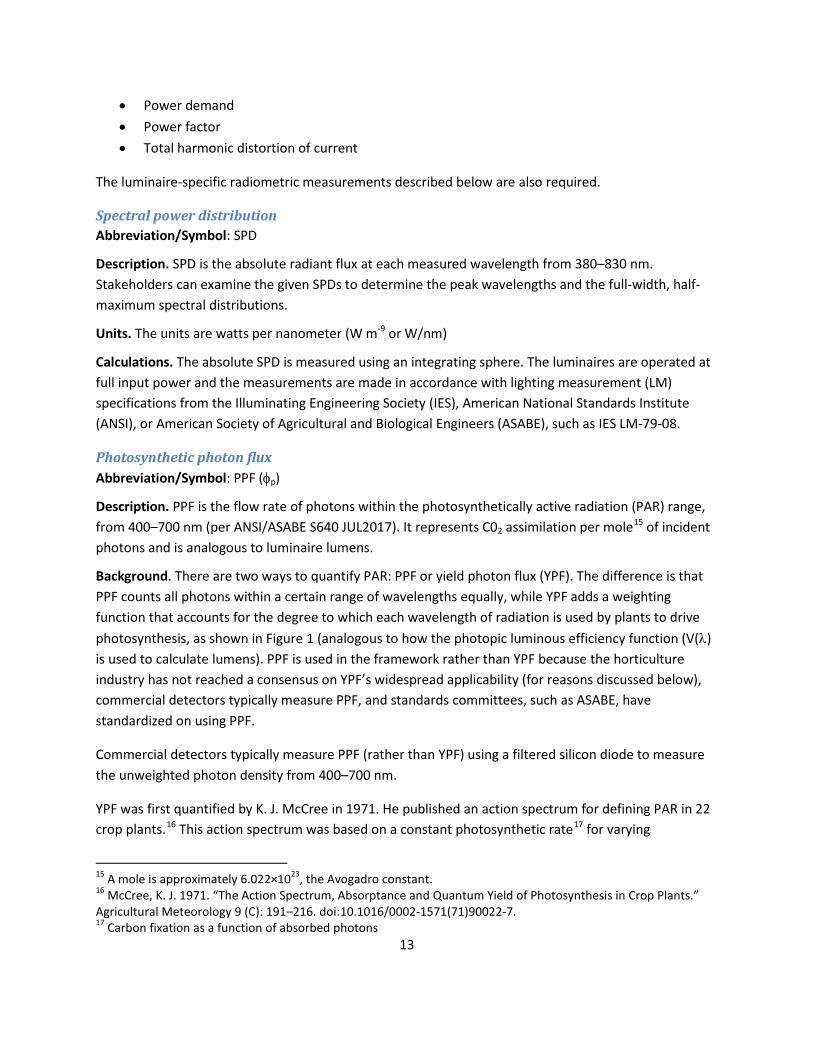
Background. There are two ways to quantify PAR: PPF or yield photon flux (YPF). The difference is that PPF counts all photons within a certain range of wavelengths equally, while YPF adds a weighting function that accounts for the degree to which each wavelength of radiation is used by plants to drive photosynthesis, as shown in Figure 1 (analogous to how the photopic luminous efficiency function (V(λ) is used to calculate lumens). PPF is used in the framework rather than YPF because the horticulture industry has not reached a consensus on YPF’s widespread applicability (for reasons discussed below), commercial detectors typically measure PPF, and standards committees, such as ASABE, have standardized on using PPF.
Commercial detectors typically measure PPF (rather than YPF) using a filtered silicon diode to measure the unweighted photon density from 400–700 nm.
YPF was first quantified by K. J. McCree in 1971. He published an action spectrum for defining PAR in 22 crop plants.16 This action spectrum was based on a constant photosynthetic rate17 for varying
15 A mole is approximately 6.022×10²³, the Avogadro constant. 16 McCree, K. J. 1971. “The Action Spectrum, Absorptance and Quantum Yield of Photosynthesis in Crop Plants.” Agricultural Meteorology 9 (C): 191–216. doi:10.1016/0002-1571(71)90022-7. 17 Carbon fixation as a function of absorbed photons

14
narrowband spectra within a range of irradiances spanning from 16–150 μmol m-2 sec-1 encompassing the wavelength range of 350–750 nm. The average action spectrum across all measured crops was the relative quantum efficiency (RQE) and was used to calculate YPF. McCree compared the predicted photosynthetic rate to measured rates under several broadband light sources and found that the action spectrum was additive. YPF, however, has not been accepted as a consensus metric for several reasons. For example, it has been measured over only low-to-medium irradiance levels and on single leaves rather than the whole plant, and the difference in short-wavelength sensitivity among the tested crop plants does not allow for accurate predictions for specific plants using broadband light sources.
In comparison to the unweighted sensitivity function used to calculate PPF, the RQE sensitivity function has attenuated sensitivity to short wavelengths, and the resulting YPF values are about 7% lower on average than PPF.18
PPF (with units of µmol s-1) and PPFD (with units of µmol m-2 s-1) have been recommended as part of a set of standard metrics in a recent standards document (ANSI/ASABE S640 JUL2017).
Figure 1: Relative sensitivity functions for PPF (green line) and YPF (blue line)
Units. The units are micromoles per second (µmol × s-1).
Calculations. PPF is calculated by converting the radiant flux at each wavelength in the absolute SPD to photon flux and integrating the photon flux from 400–700 nm.
18 2014 LRC report to NRCan on horticultural lighting testing

15
Photosynthetic photon efficacy Abbreviation/Symbol: PPE (Kp)
Description. PPE is the ratio of the luminaire’s measured PPF to its power demand. It is analogous to luminaire efficacy (lumens per watt).
Background. Nelson and Bugbee19 tested a variety of HID, LED and fluorescent luminaires and published the PPE (µmol J-1) of each luminaire. In 2014, the most efficacious HPS luminaires had a PPE of 1.70 µmol J-1 (range: 0.94–1.70 µmol J-1) as did one of ten LED luminaires tested (range: 0.89–1.70 µmol J-1). In a recent U.S. Department of Energy (DOE) report,20 the “best-in-class” PPE is 2.5 µmol J-1 for LED luminaires available in 2017, and 2.1 µmol J-1 for double-ended HPS luminaires available in 2017.
Units. The units are micromoles per joule (µmol × J-1).
Calculations. PPE is calculated by dividing the measured PPF by the measured input power.
Percentage of the total measured SPD in the PAR range Abbreviation/Symbol: PPF% (φp%)
Description. The percentage of the total measured SPD (PPF% or φp%) in the PAR range (400–700 nm). This metric has been proposed by researchers21 to inform stakeholders of the luminaire’s efficiency in producing optical radiation in the PAR range.
Units. This is a unitless ratio.
Calculation. PPF% is calculated by dividing the integrated photon flux between 400–700 nm by the integrated photon flux for the entire SPD (e.g., between 380–830 nm). A comparison across multiple SPDs is only accurate if the wavelength range is consistent among the SPDs.
Phytochrome photostationary state Abbreviation/Symbol: PSS
Description. PSS is a measure of the SPD’s impact on phytochrome, a photo-activated plant protein which regulates photomorphogenic responses, seed germination, flowering, and photosynthesis.
Background. Phytochrome is a bistable photo pigment that regulates photomorphogenic responses, as well as seed germination, flowering and photosynthesis. The active form of phytochrome is Pfr (far-red absorbing); the inactive form is Pr (red absorbing). Sager et. al. (1988)22 formulated a metric known as photosynthetic photostationary state (PSS) to evaluate the relative activity of phytochrome. A higher
19 Nelson, Jacob A., and Bruce Bugbee. 2014. “Economic Analysis of Greenhouse Lighting: Light Emitting Diodes vs. High Intensity Discharge Fixtures.” PLoS ONE 9 (6). doi:10.1371/journal.pone.0099010. 20 Stober, Kelsey, Kyung Lee, Mary Yamada, and Morgan Pattison. 2017. “Energy Savings Potential of SSL in Horticultural Applications.” 21 Both et al., 2017. “Proposed Product Label for Electric Lamps Used in the Plant Sciences.” HortTechnology August 2017 vol. 27 no. 4 544-549 22 Sager, J. C., W. O. Smith, J. L. Edwards, and K. L. Cyr. 1988. “Photosynthetic Efficiency and Phytochrome Photoequilibria Determination Using Spectral Data.” Transactions of the ASAE. doi:10.13031/2013.30952.

16
PSS value indicates that the SPD will stimulate more Pr than Pfr. Light sources with higher percentages of flux in the far-red waveband (700–800 nm), like sunlight (PSS: 0.73) and incandescent lamps (PSS: 0.67), have lower PSS values than HPS (PSS: 0.86) and MH (PSS: 0.80) light sources.23
Units. This is a unitless ratio.
Calculations. PSS is calculated by dividing the integrated SPD multiplied by the Pr function at each wavelength by the integrated SPD multiplied by the sum of the Pr + Pfr function at each wavelength.
Photosynthetic photon intensity distribution Abbreviation/Symbol: Ip
Description. The photosynthetic photon intensity distribution shows the spatial distribution of the photosynthetic photon intensity measurements in two 2-D planes through the maximum intensity value. Photosynthetic photon intensity distributions with a “batwing” shape (lower intensities below the luminaire and higher intensities at the higher vertical angles) provide a more uniform PPFD over a wider area, which is a typical goal of lighting layouts.
Units. The units are micromoles per steradian per second (µmol ×sr-1 x s-1).
Calculations. The photosynthetic photon intensity is the PPF within a given solid angle. It is calculated by converting the luminous intensity values given in an IES file to photosynthetic photon intensity values using the absolute SPD data.
Relative SPD and percentage of radiant flux at different vertical angles Abbreviation/Symbol: N/A
Description. This is a measure of the color uniformity of the luminaire. It is calculated and presented in two ways: a table of the percentage of radiant flux at different vertical angles and a graphic of relative SPD at different vertical angles presented as a chart. Stakeholders can use this information to assess how similar the SPD will be for a plant directly under the luminaire versus one at a distance from nadir.
Units. The metrics are percentages and ratios, so they are unitless.
Calculations. The measured SPDs at each of six angles are normalized such that the maximum radiant power is set equal to 1. The integrated radiant flux is integrated across specified wavebands (UV: 350– 400 nm; blue: 400–500 nm; red: 600–700 nm; far-red: 700–800 nm) and the percentages of radiant flux and blue/red and red/far-red ratios are calculated for each vertical angle.

17
Application-specific metrics Horticultural luminaire comparisons should not be made solely at a luminaire level, but also at a system level when the luminaires are arranged to meet the applications requirements.
Photosynthetic photon flux density Abbreviation/Symbol: PPFD
Description. PPFD, the amount of photosynthetic photon flux incident on an area, is the prevailing metric for irradiance levels. PPFD is measured in PPF per square meter, and is analogous to photopic illuminance (measured in lux). Like illuminance, the average PPFD is often used as a target light level criterion for growing crops. PPFD is used as an intermediate metric to calculate luminaire system application efficacy (LSAE) and is used as an equivalency criterion to determine the luminaire quantity used in life-cycle cost analysis (LCCA) calculations. PPFD and duration of exposure are used to calculate the daily light integral (DLI), and a sufficiently high PPFD is needed to provide the necessary DLI within a certain time period each day.
Background. A primary use of the PPFD metric is as an intermediate metric for stakeholders to calculate DLI. Supplemental lighting needs are often based on DLI, the 24-hour dose of PPFD required for photosynthesis.23 It is a function of PPFD and duration, and is given in units of mol m-2 day-1.24 In other words, PPFD and duration can be traded off against one another to provide crops with a target DLI. Figure 2 shows the calculated DLI for 5 target PPFD levels (75, 150, 225, 300, 500 and 1000 μmol m-2 sec-
1) and three durations (12, 16 and 20 hours). For example, a target DLI of 10 is achievable with target PPFDs of 150, 225 and 300 μmol m-2 sec-1, by using a different duration.
Purdue Extension recommends DLI levels for various crops grown in greenhouses.25 The DLI required for minimum acceptable quality ranges from 2 mol m-2 day-1 to 10 mol m-2 day-1, depending on the crop. Good quality results require a DLI of 4 – 14 mol m-2 day-1.
Units. The units of PPFD are μmol m-2 sec-1.
Calculations. PPFD is calculated as the PPF incident on a surface area, divided by the area of the surface in square meters. Interreflections and obstructions are not considered in the calculations. Photometric simulations are used to determine the number of luminaries needed to provide the required PPFD.
23 Torres, Ariana P., and Roberto G. Lopez. 2010. “Commercial Greenhouse Production - Measuring Daily Light Integral in a Greenhouse.” Purdue Extension. https://www.extension.purdue.edu/extmedia/ho/ho-238-w.pdf. 24 DLI is calculated by multiplying the average hourly PPFD over 24 hours (under both supplemental lighting and in darkness) by 0.0864 (86,400 seconds per day divided 1,000,000). 25 Torres, Ariana P., and Roberto G. Lopez. 2010. “Commercial Greenhouse Production - Measuring Daily Light Integral in a Greenhouse.” Purdue Extension. https://www.extension.purdue.edu/extmedia/ho/ho-238-w.pdf.

18
Figure 2: Calculated DLI values for a range of PPFD levels and durations
PPFD uniformity Abbreviation/Symbol: N/A
Description. The target minimum-to-average PPD. It is an intermediate metric used in the LSAE method, described below.
Background. PPFD uniformity on the work plane is often specified as an important design consideration, but a target uniformity is rarely provided, nor the reasoning behind a recommended value. Fisher et. al. (2001) recommend a minimum-to-maximum ratio of 0.70.26 A common rule of thumb in the horticultural lighting industry is that a preferred minimum-to-average PPFD uniformity is 0.8:1, and a less-preferred minimum-to-average uniformity is 0.6:1.
Units. This is a ratio, so it is unitless.
Calculations. It is calculated by dividing the minimum PPFD by the average PPFD.
Luminaire system application efficacy Abbreviation/Symbol: LSAE
Description. The LRC developed an LSAE method to compare luminaire quantities and application efficacies at various PPFD levels and mounting heights. LSAE is the system efficacy of a luminaire layout, at a given mounting height, that meets the given PPFD and uniformity requirements for a given growing area. Higher LSAE values indicate that the given luminaire layout is more effective at meeting the target 26 Fisher, Paul, Caroline Donnelly, and James Faust. 2001. “Evaluating Supplemental Light for Your Greenhouse.”
19
requirements. A table of LSAE values for a range of PPFD values (75, 150, 225, 300, 500 and 100 μmol m-
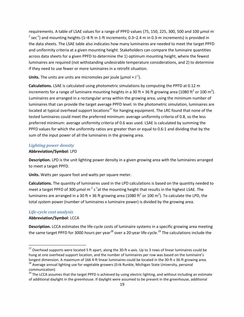
2 sec-1) and mounting heights (1–8 ft in 1-ft increments; 0.3–2.4 m in 0.3-m increments) is provided in the data sheets. The LSAE table also indicates how many luminaires are needed to meet the target PPFD and uniformity criteria at a given mounting height. Stakeholders can compare the luminaire quantities across data sheets for a given PPFD to determine the 1) optimum mounting height, where the fewest luminaires are required (not withstanding undesirable temperature considerations, and 2) to determine if they need to use fewer or more luminaires in a retrofit situation.
Units. The units are units are micromoles per joule (µmol × J-1).
Calculations. LSAE is calculated using photometric simulations by computing the PPFD at 0.12 m increments for a range of luminaire mounting heights in a 30 ft × 36 ft growing area (1080 ft2 or 100 m2). Luminaires are arranged in a rectangular array within the growing area, using the minimum number of luminaires that can provide the target average PPFD level. In the photometric simulation, luminaires are located at typical overhead support locations27 for hanging equipment. The LRC found that none of the tested luminaires could meet the preferred minimum: average uniformity criteria of 0.8, so the less preferred minimum: average uniformity criteria of 0.6 was used. LSAE is calculated by summing the PPFD values for which the uniformity ratios are greater than or equal to 0.6:1 and dividing that by the sum of the input power of all the luminaires in the growing area.
Lighting power density Abbreviation/Symbol: LPD
Description. LPD is the unit lighting power density in a given growing area with the luminaires arranged to meet a target PPFD.
Units. Watts per square foot and watts per square meter.
Calculations. The quantity of luminaires used in the LPD calculations is based on the quantity needed to meet a target PPFD of 300 μmol m-2 s-1at the mounting height that results in the highest LSAE. The luminaires are arranged in a 30 ft × 36 ft growing area (1080 ft2 or 100 m2). To calculate the LPD, the total system power (number of luminaires x luminaire power) is divided by the growing area.
Life-cycle cost analysis Abbreviation/Symbol: LCCA
Description. LCCA estimates the life-cycle costs of luminaire systems in a specific growing area meeting the same target PPFD for 3000 hours per year28 over a 20-year life-cycle.29 The calculations include the
27 Overhead supports were located 5 ft apart, along the 30-ft x-axis. Up to 3 rows of linear luminaires could be hung at one overhead support location, and the number of luminaires per row was based on the luminaire’s longest dimension. A maximum of 166 4-ft linear luminaires could be located in the 30-ft x 36-ft growing area. 28 Average annual lighting use for vegetable growers (Erik Runkle, Michigan State University, personal communication) 29 The LCCA assumes that the target PPFD is achieved by using electric lighting, and without including an estimate of additional daylight in the greenhouse. If daylight were assumed to be present in the greenhouse, additional

20
LPD, rate of return30 and payback estimates. LCCA requires luminaire price information as well as estimates of replacement and failure rates and costs.
Units. Cost: U.S. dollar; cost per area: $ per square foot and $ per square meter; LPD: watts per square foot and watts per square meter; annual energy use per area: kilowatt hours per square foot per year and kilowatt hours per square meter per year; annual energy cost per area: dollars per square foot per year and dollar per square meter per year; rate of return: percentage; payback: years; total payments over 20 years: dollars using present worth.
Calculations. LCCA incorporates the following information for each system for the same target PPFD: luminaire costs, installation costs, installed luminaire cost density, LPD, and annual energy use density. The LCCA provides the following group of metrics: annual energy cost density, rate of return and payback periods for the system compared to a base case 600 W and 1000 W HPS systems, and estimated cumulative costs over 20 years. The quantity of luminaires used in the LSAE is the number needed at the mounting height that results in the highest LSAE for a target PPFD of 300 μmol m-2 s-1.
An LCCA was performed to estimate the life-cycle costs of luminaire systems in a 30 ft × 36 ft growing area (1080 ft2 or 100 m2) meeting the same target PPFD for 3000 hours per year31 over a 20-year life-cycle.32
The number of luminaires used for each luminaire type in the LCCA is based on the layout that results in the highest LSAE for the target PPFD. A discount rate of 3% is used. A 1000 W HPS system (P.L. Light Systems Med NXT LP 1000 W Beta) and a 600 W HPS system (P.L. Light Systems PL2000 HPS 600 W 240V with SON-T PIA lamp, tested in 2013) are used as base cases, both mounted at a height of 6 ft above the crop canopy.
To account for differences in cost of electricity for different regions, the LCCA was performed with low ($0.1048/kWh33) and high ($0.20/kWh) energy rates.
The LCCA calculates the following group of metrics: annual energy cost density, rate of return and payback periods for the system compared to a 600 W and 1000 W HPS system, and estimated cumulative costs over 20 years.
The below assumptions are used in the LCCA calculations and are based on 2017 RSMeans data.34
energy use as a result from luminaire shading would have to be considered, as well as dimming assumptions and the cost of additional control gear for monitoring light levels, and dimming the luminaires. 30 Rate of return is calculated as the average annual cash flow for a given energy rate and base case divided by the initial installed cost. 31 Average annual lighting use for vegetable growers (Erik Runkle, Michigan State University, personal communication) 32 The LCCA assumes that the target PPFD is achieved by using electric lighting, and without including an estimate of additional daylight in the greenhouse. If daylight were assumed to be present in the greenhouse, additional energy use as a result from luminaire shading would have to be considered, as well as dimming assumptions and the cost of additional control gear for monitoring light levels, and dimming the luminaires. 33 Average retail price of electricity in Q2 2017. https://www.eia.gov/electricity/data/browser/#/topic/7?agg=2,0,1&geo=g&freq=M

21
• Labor rate for electrician to install one luminaire (any light source): $69 • Labor rate to replace one lamp, or one lamp and reflector: $16 • P.L. Light Systems recommends cleaning reflectors every year. Labor rate to clean one HID
reflector: $30; Labor rate to clean one LED luminaire: $6 • A 2% annual lamp failure rate was used for the HID LCCA. For the LED systems, the LCCA
includes a sensitivity analysis with 1% failure rates or 25% failure rates occurring at year 10. The total payments with both failure rates are shown in the plotted figures; however, the total payments cell in the LCCA summary table shows the cumulative costs with a less-conservative 1% failure rate assumption.
Table 2: HID lamp and reflector costs used in LCCA
Luminaire Brand Source Lamp Rated
Lamp Life (Hours)35
Lamp Cost
Rated Reflector Life
(Hours)
Reflector Cost
1000 W HPS Gavita HPS Gavita ProPlus 1000 W
EL DE HPS 5,000 $135 10,000 $53
1000 W HPS
P.L. Light
Systems HPS
Ushio HiLux Gro Super HPS with optimized blue
and red spectrum 10,000 $120 10,000 $40
1000 W MH
P.L. Light
Systems MH
Ushio HiLux Gro Super MH with optimized blue
and red spectrum 10,000 $120 10,000 $110
600 W HPS36
P.L. Light
Systems HPS SON-T PIA 12,000 $32 10,00037 $40
Luminaire data sheets The metrics listed above, plus additional information, are presented on a standardized luminaire data sheet. The recommended two-page data sheet format is shown in the “Appendix B: Data sheets” and includes:
• The luminaire brand, model number and catalog number. • A photograph of the energized luminaire. • The measured electrical characteristics including input voltage, power, THDi and PF, and light
output characteristics such as PPF, PPE, PPF%, and PSS are shown on the top. • A photosynthetic photon flux comparison, showing the given luminaire’s PPF value compared to
values for the range of tested horticultural luminaires.
34 https://www.rsmeans.com 35 Rated lamp life is based on the luminaire manufacturer’s recommended HID lamp replacement interval 36 Purchased and tested in 2013. Measured PPF: 926 μmol s-1, Kp: 1.28 μmol J-1 37 Lamp will be replaced when the reflector is replaced.

22
• The photosynthetic photon flux efficacy comparison shows the given luminaire’s PPF efficacy compared to the range of efficacies for all the tested horticultural luminaires.
• An LSAE comparison table, which provides LSAE values for a range of PPFD values (75, 150, 225, 300, 500 and 100) and mounting heights (1–8 ft in 1-ft increments; 0.3–2.4 m in 0.3-m increments). The table also indicates how many luminaires are needed to meet the target PPFD and uniformity criteria at a given mounting height. Stakeholders can compare the luminaire quantities across data sheets for a given PPFD to determine the mounting height at which the fewest luminaires are required38 and if they need to use fewer or more luminaires when upgrading from existing luminaires.
• The absolute SPD. • An LCCA table, which provides the estimated cumulative costs for both low and high energy
rates for three systems: the given luminaire and 600 W HPS and 1000 W HPS base cases. • Iso-PPFD contours, useful for comparing irradiances and uniformity at a given mounting height. • The plot of photosynthetic photon intensity distribution (Ip), which shows the spatial distribution
using two dimensional planes (with units of μmol sr-1 s-1). Similar to the iso-PPFD contours, the photosynthetic intensity distribution is helpful for stakeholders who wish to evaluate the spatial distribution of the luminaire. A red line shows a horizontal slice through the vertical angles where the maximum candela value occurs. A blue line represents the vertical slice through the luminaire's center at the horizontal angle with the maximum candela angle. Each of the four rings in the polar diagram represents a 25% change in luminous intensity, with the maximum candela value represented by the outer ring. Each radiating line represents a 10° angular increment.
• Color uniformity, presented in two ways. First, the relative SPDs measured at multiple vertical angles are shown. Stakeholders can compare the color uniformity by examining the peak wavelength ratios for consistency. (e.g., Is the 450 nm / 660 nm ratio the same at 0° vertical as at other vertical angles?) Second, a table of radiant flux percentages in common wavebands (UV: 350–400 nm; blue: 400–500 nm; red: 600–700 nm; far-red: 700–800 nm), as well as the blue/red and red/far-red ratios are presented for different vertical angles. Stakeholders can examine the radiant flux percentages and ratios to see if they vary meaningfully across the measured vertical angles that represent their growing area.
Purchasing and testing luminaires In late 2016, the LRC selected luminaires for the study, according to the manufacturers named by the growers in the online survey detailed above. At the time of selection, horticultural lighting manufacturers typically made one of two form factors: a mid- to high-power standalone product or a “lightbar” with a linear form factor and end-to-end couplings to create continuous rows of lighting. One manufacturer, Illumitex, had both form factors available. The luminaires shown in Table 3 were selected
38 It is left to the grower to make sure the mounting height is high enough to prevent thermal damage of the crop.
23
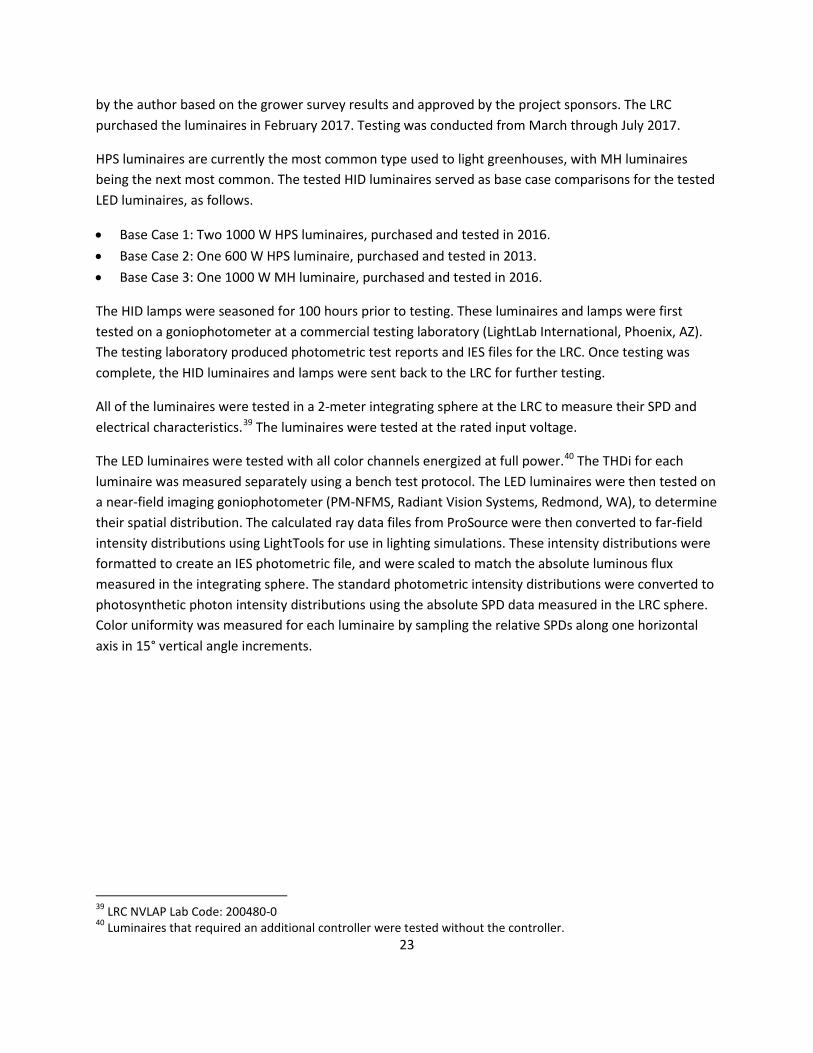
by the author based on the grower survey results and approved by the project sponsors. The LRC purchased the luminaires in February 2017. Testing was conducted from March through July 2017.
HPS luminaires are currently the most common type used to light greenhouses, with MH luminaires being the next most common. The tested HID luminaires served as base case comparisons for the tested LED luminaires, as follows.
• Base Case 1: Two 1000 W HPS luminaires, purchased and tested in 2016. • Base Case 2: One 600 W HPS luminaire, purchased and tested in 2013. • Base Case 3: One 1000 W MH luminaire, purchased and tested in 2016.
The HID lamps were seasoned for 100 hours prior to testing. These luminaires and lamps were first tested on a goniophotometer at a commercial testing laboratory (LightLab International, Phoenix, AZ). The testing laboratory produced photometric test reports and IES files for the LRC. Once testing was complete, the HID luminaires and lamps were sent back to the LRC for further testing.
All of the luminaires were tested in a 2-meter integrating sphere at the LRC to measure their SPD and electrical characteristics.39 The luminaires were tested at the rated input voltage.
The LED luminaires were tested with all color channels energized at full power.40 The THDi for each luminaire was measured separately using a bench test protocol. The LED luminaires were then tested on a near-field imaging goniophotometer (PM-NFMS, Radiant Vision Systems, Redmond, WA), to determine their spatial distribution. The calculated ray data files from ProSource were then converted to far-field intensity distributions using LightTools for use in lighting simulations. These intensity distributions were formatted to create an IES photometric file, and were scaled to match the absolute luminous flux measured in the integrating sphere. The standard photometric intensity distributions were converted to photosynthetic photon intensity distributions using the absolute SPD data measured in the LRC sphere. Color uniformity was measured for each luminaire by sampling the relative SPDs along one horizontal axis in 15° vertical angle increments.
39 LRC NVLAP Lab Code: 200480-0 40 Luminaires that required an additional controller were tested without the controller.

24
Table 3: Purchased HID and LED luminaires
Source, Brand, Rated Wattage Model Name/Catalog Number Single-unit price
HPS, Gavita, 1000 1000 W HPS Grow Light
Pro 1000e DE US 120-240 (with one double-ended Gavita HPS lamp)
$540
HPS, P.L. Light, 1000 1000 W HPS with Beta reflector
Med NXT LP 1000 W Beta (with one double-ended Ushio HPS lamp)
$525
MH, P.L. Light, 1000 1000 W MH with Maxima reflector
MEDSLA/MH/1000 W/277V USH (with one single-ended Ushio MH lamp)
$569
LED, GE, 31 Arize Lynk GEHL48HPKB1 $245
LED, Heliospectra, 630 LX601C $2,400
LED, Hubbell, 425 Cultivaire CGS-4-FSG-U-W-E-U-C6TL15 $911
LED, Illumitex, 63 Eclipse W ESW14812F3UD $383
LED, Illumitex, 300 PowerHarvest W PHW5F3URC10P120 $834
LED, Lumigrow, 300 Pro325e $1,100
LED, OSRAM, 600 ZELION HL300 $1,800
LED, Philips, 200 GreenPower LED toplighting Deep Red-White-Far Red-Medium Blue $955
LED, P.L. Light, 320 HortiLED TOP-150° distribution angle-120-277V-Full Spectrum-0-10 V dimming
$1,186
LED, Sunlight Supply, 450 AgroLED 720 Dio-Watt Full Spectrum Low Pro 120 - 240 Volt 90° Optics $765
Results Luminaire-specific test results Detailed test results for each luminaire are provided in “Appendix B: Data sheets.” The results are summarized below.
Electrical results Table 3 shows the results of the sphere and bench tests with regard to electrical parameters. The 1000 W HPS luminaires are color-coded in blue, the 1000 W MH luminaire is color-coded in red, the 600 W HPS is color-coded in green, and the LED luminaires are color-coded in black type in tables and gray bars in the charts.

25
All of the tested LED luminaires had a lower power demand than any of the tested HID luminaires. All of the tested luminaires had measured THDi and PF values that would meet Design Lights Consortium (DLC) technical requirements41 (PF ≥ 0.90, THDi ≤ 20%).
Table 4: Measured power, THDi, and PF for tested luminaires
Source, Brand, Rated Wattage Input Volts (V)
Measured Power
(W)
Measured THDi (%) Measured PF
Base Case 1 HPS, Gavita, 1000 239.9 1069.3 7.5 0.99
Base Case 1 HPS, P.L. Light, 1000 239.8 1057.3 5.4 0.98
Base Case 2 HPS, P.L. Light, 600* 240.1 690.2 Not measured 0.98
Base Case 3 MH, P.L. Light, 1000 277.0 1042.2 2.6 0.99
LED, GE, 31 120.1 30.0 11.5 0.99
LED, Heliospectra, 630 119.8 595.3 7.3 0.99
LED, Hubbell, 425 239.7 357.5 7.0 0.99
LED, Illumitex, 63 120.1 51.7 9.7 0.99
LED, Illumitex, 300 119.8 268.1 3.6 1.00
LED, Lumigrow, 300 119.8 299.9 2.9 1.00
LED, OSRAM, 600 119.9 373.942 5.1 1.00
LED, Philips, 200 240.0 194.7 7.2 1.00
LED, P.L. Light, 320 240.0 330.4 13.5 0.95
LED, Sunlight Supply, 450 119.9 414.1 7.9 0.99
*This luminaire was purchased and tested in 2013. THDi was not measured.
Radiometric results Table 4 shows the calculated PPF (φp), YPF, PPE (Kp), PPF% (φp%), and PSS for each luminaire.
41 https://www.designlights.org/solid-state-lighting/qualification-requirements/technical-requirements/ 42 This is the measured power without using the controller.

26
Table 5: Measured PPF, YPF, PPE and PSS tested luminaires = higher PPE than either 1000 W HPS luminaire = higher PPE than 600 W HPS luminaire = higher PPE than 1000 W MH luminaire
Source, Brand, Rated Power
PPF φp (µmol s-1)
YPF (µmol s-1)
PPE Kp
(µmol J-1)
PPF% φp%
PSS
Base Case 1 HPS, Gavita, 1000
1837 1748 1.72 76.7 0.84
Base Case 1 HPS, P.L. Light, 1000
1801 1716 1.70 77.2 0.85
Base Case 2 HPS, P.L. Light, 600*
926 881 1.34 75.0 0.85
Base Case 3 MH, P.L. Light, 1000
866 747 0.83 84.3 0.77
LED, GE, 31 79 70 2.64 99.9 0.88 LED, Heliospectra, 630 673 618 1.13 82.3 0.80 LED, Hubbell, 425 736 649 2.06 96.9 0.85 LED, Illumitex, 63 89 80 1.72 99.4 0.88 LED, Illumitex, 300 475 421 1.77 99.6 0.87 LED, Lumigrow, 300 540 475 1.80 99.4 0.87 LED, OSRAM, 600 788 712 2.11 99.7 0.88 LED, Philips, 200 504 456 2.59 99.5 0.88 LED, P.L. Light, 320 696 607 2.11 98.8 0.86 LED, Sunlight Supply, 450 575 512 1.39 96.9 0.87 *This luminaire was purchased and tested in 2013.
None of the LED horticultural luminaires could meet or exceed the PPF or YPF values produced by any of the tested 1000 W HPS, 600 W HPS, or 1000 W MH luminaires. On average, the tested LED luminaires had 28% of the PPF of the tested 1000 W HPS luminaires (median: 31%), 56% of the PPF of the tested 600 W HPS luminaire (median: 60%), and 64% of the PPF of the tested 1000 W MH luminaire.
Table 6 shows the number of LED luminaires with higher PPE than the three base cases. Most of the tested LED luminaires had higher PPE than both of the tested 1000 W HPS luminaires and the tested 600 W HPS luminaire. All of the tested LED luminaires had higher PPE than the tested 1000 W MH luminaire.
Table 6: Number of LED luminaires with higher PPE than the base cases.
Base Case Number of tested LED luminaires with higher PPE than base case
1 1000 W HPS 8 of 10 2 600 W HPS 9 of 10 3 1000 W MH 10 of 10

27
Almost all of the tested LED luminaires had PPF% that were close to 100%, except for one LED luminaire that had more flux in the far-red region. The HPS luminaires had PPF% of about 76% because of some flux in the infrared region, while the tested MH luminaire had a PPF% of about 84% because of some flux in the ultraviolet and infrared regions.
As discussed in the Framework section above, PAR can be calculated using YPF or PPF. As shown in Figure 3, YPF was about 7% lower than PPF on average, but there was a very strong correlation between the two metrics (R2=0.996).
Figure 3: YPF vs. PPF.
Color uniformity results The tested 1000 W HPS luminaires showed minor variations in the spectral ranges at different vertical angles. The UV, blue, red, and far-red waveband percentages at different vertical angles varied by less than1%, and the blue/red and red/far-red waveband ratios varied by 10% or less.
The tested 1000 W MH luminaire had more variability. At higher vertical angles, the UV waveband percentage decreased by less than 1%, the blue waveband percentage decreased 6%, the red waveband percentage increased 4%, and the far-red waveband percentage increased less than 1%. As a result, the blue/red waveband ratio decreased 35% at higher vertical angles. The red/far-red ratio waveband decreased by 2%.
Six of the ten tested LED luminaires had blue, red or far-red waveband percentage variations greater than 5% in one or more spectral ranges. For these luminaires, the red waveband percentages typically varied the most. As a result, the blue/red waveband ratio changed by 35% on average (range: 0.64 – 1.63), and the red/far-red waveband ratio changed by 17% on average (range: 0.34 – 1.9). It is uncertain if the non-uniform color results within the beam spread have a meaningful impact on plant growth, but the LRC believes this information is useful for comparison purposes.

28
Application-specific test results For each of the application calculations, a target PPFD of 300 µmol m-2 s-1 was used. However, two luminaires (LED, GE, 30 and LED, Illumitex, 52) were not able to achieve this PPFD, even at the maximum number of luminaires that could fit into the simulated greenhouse due to physical constraints. For these two luminaires, a lower PPFD of 75 µmol m-2 s-1 was used.
Number of luminaires needed and lighting power density Figure 4 shows the median number of luminaires required and subsequent LPD by light source to meet a target PPFD of 300 µmol m-2 s-1.
Figure 4: Boxplots show the median luminaire quantity and LPD by light source for measured HID and LED horticultural luminaires meeting a target PPFD of 300 µmol m-2 s-1.
Table 7 provides the number of LED luminaires with lower LPD than the base cases. A lower LPD results in less energy use, all else being equal.
Table 7: Number of LED luminaires with lower LPD than the base cases.
Base Case Number of tested LED luminaires with lower LPD than base case Target PPFD of 300 μmol m-2 s-1 Target PPFD of 75 μmol m-2 s-1
1 1000 W HPS 4 of 8 2 of 2 2 600 W HPS 7 of 8 2 of 2 3 1000 W MH 8 of 8 2 of 2

29
Luminaire System Application Efficacy Table 8 shows the number of LED luminaire models with a higher maximum LSAE than the base cases.
Table 8: Number of LED luminaires with higher maximum LSAE than the base cases.
Base Case Number of tested LED luminaires with higher maximum LSAE than base case Target PPFD of 300 μmol m-2 s-1 Target PPFD of 75 μmol m-2 s-1
1 1000 W HPS 2 of 8 1 of 2 2 600 W HPS 4 of 8 1 of 2 3 1000 W MH 8 of 8 2 of 2
Life-Cycle Cost Analysis Figure 5 shows the median cumulative costs over 20 years and median rate of return by light source, for high and low energy rates, for a target PPFD of 300 μmol m-2 s-1. Economic results are summarized in Table 9.
(a)
(b)
Figure 5: Boxplots show median total payments over 20 years and rate of return by light source for measured HID and LED horticultural luminaires meeting a target PPFD of 300 µmol m-2 s-1. (a) Median total payments over 20 years by light source for low and high energy rates. (b) Median rate of return by light source compared to 600 W HPS with high and low energy rates. Asterisks represent outliers.

30
Table 9: Summary of economic results.
Base Case Economic results Target PPFD of 300 μmol m-2 s-1 Target PPFD of 75 μmol m-2 s-1
1 1000 W HPS
Three of the eight tested LED luminaires had a lower 20-year life-cycle cost than either of the 1000 W HPS luminaires, and they had a higher rate of return. None of the eight tested LED systems had a payback range shorter than 20 years at the low energy rate. At the high energy rate, two tested LED systems had payback range of 18 to 20 years, with a longer payback period for the other six luminaires.
One of the two tested LED luminaires had a lower 20-year life-cycle cost than one of the tested 1000 W HPS luminaires, when the energy rate was high. Both tested LED systems had a positive rate of return, ranging from 1.5% to 6.3%. None of the two tested LED systems had a payback range shorter than 20 years, at either energy rate.
2 600 W HPS Seven of the eight tested LED luminaires had a lower 20-year life-cycle cost than any of the 600 W HPS luminaires, when the energy rate was high. When the energy rate was low, six of the eight tested LED luminaires had a lower 20-year life-cycle cost than any of the 600 W HPS luminaires. Seven of the eight tested LED luminaires had a positive rate of return at both energy rates, ranging from 5% to 14.9%. Replacing the 600 W HPS system with a 1000 W HPS system resulted in the highest rates of return (13.3% - 46.5% depending on energy rate) and a payback period of one year.
One of the two tested LED luminaires had a lower 20-year life-cycle cost than one of the tested 1000 W HPS luminaires, when the energy rate was high. Both tested LED systems had a positive rate of return, ranging from 2.3% to 7.7%. Only one of the two tested LED system had a payback period shorter than 20 years, and only if a high energy rate was used.
3 1000 W MH
Seven of the eight tested LED luminaires had a lower 20-year life-cycle cost than the 1000 W MH luminaire. Rate of return and payback periods relative to the 1000 W MH were not calculated.
Both tested LED luminaires had a lower 20-year life-cycle cost than the 1000 W MH luminaire. Rate of return and payback periods relative to the 1000 W MH were not calculated.
Tables 10 and 11 below show the median quantity, lighting power density (LPD), maximum LSAE for any PPFD / mounting height combination, and the estimated total payments over 20 years for the tested HID and LED horticultural luminaires.

31
Table 10: Average luminaire quantity, LPD, maximum LSAE, and total payments over 20 years, for low and high energy rates, for measured HID and LED horticultural luminaires meeting a target PPFD of 300 µmol m-2 s-1. = Lower LPD, higher Max. LSAE, lower cost than either 1000 W HPS system = Lower LPD, higher Max. LSAE, lower cost than 600 W HPS system = Lower LPD, higher Max. LSAE, lower cost than 1000 W MH system
Source, Brand, Rated Power
Quantity to meet 300 µmol m-2 s-1
LPD (W ft-2) [W m-2]
Max. LSAE (µmol J
-1)
Total Payments ($0.10/kWh)
Total Payments ($0.20/kWh)
Base Case 1 HPS, Gavita, 1000 24 24 [256] 1.31 $198,503 $307,528
Base Case 1 HPS, P.L. Light, 1000 24 23 [253] 1.27 $167,128 $274,930
Base Case 2 HPS, P.L. Light, 600 50 32 [344] 1.12 $238,972 $385,538
Base Case 3 MH, P.L. Light, 1000 45 43 [467] 0.66 $325,603 $524,844
LED, Heliospectra, 630 70 39 [415] 0.71 $375,210 $552,241
LED, Hubbell, 425 66 22 [235] 1.23 $181,365 $281,603
LED, Illumitex, 300 99 25 [265] 1.09 $222,976 $335,733
LED, Lumigrow, 300 90 25 [269] 1.09 $240,208 $354,874
LED, OSRAM, 600 63 22 [235] 1.34 $234,376 $334,448 LED, P.L. Light, 320 68 21 [224] 1.23 $197,081 $292,529
LED, Philips, 200 96 17 [187] 1.56 $195,102 $274,630
LED, Sunlight Supply, 450 80 31 [330] 0.88 $229,245 $369,983
Table 11: Average luminaire quantity and total payments over 20 years, for low and high energy rates, for measured HID and LED horticultural luminaires meeting a target PPFD of 75 µmol m-2 s-1. = Lower LPD, higher Max. LSAE, lower cost than either 1000 W HPS system = Lower LPD, higher Max. LSAE, lower cost than 600 W HPS system = Lower LPD, higher Max. LSAE, lower cost than 1000 W MH system
Source, Brand, Rated Power
Quantity to meet 75 µmol m-2 s-1
LPD (W ft-2) [W m-2]
Max. LSAE
(µmol J-1)
Total Payments ($0.10/kWh)
Total Payments ($0.20/kWh)
Base Case 1 HPS, Gavita, 1000 9 9 [95] 1.30 $62,309 $102,735
Base Case 2 HPS, P.L. Light, 600 15 10 [103] 1.10 $71,691 $115,661
Base Case 3 MH, P.L. Light, 1000 15 14 [156] 0.60 $108,354 $174,948
LED, GE, 31 150 4 [45] 1.59 $81,806 $100,923
LED, Illumitex, 63 132 6 [68] 0.99 $103,706 $132,670
Daylighting simulation results During the summer months, when DLI levels are highest, supplemental lighting is usually not required. Supplemental lighting installed to meet target PPFDs at other times of the year will cause shading year-

32
round. To investigate the shading caused by horticultural luminaires, a 30-ft × 36-ft greenhouse was modeled in AGi32 as the base case. In one set of greenhouse simulations, clear glazing with a visible transmittance of 90% was used (Figure 6 left).43 In another set of simulations, diffuse glazing with a visible transmittance of 87% was used.44 A sufficient quantity of luminaires was added to the greenhouse to meet a target PPFD of 300 µmol m-2 s-1,45 (Figure 6 right), but the luminaires were assumed to be de-energized and did not contribute to the DLI in this shading simulation.
To analyze the shading effects of the tested luminaires, typical meteorological year (TMY) data for Albany, New York, a predominantly overcast climate, and San Diego, California, a predominantly clear climate, was used for each simulation. The AGi32 models were imported into Licaso,46 an annual daylight simulation tool, for analysis. Licaso simulates hourly light levels over the course of a typical year. The average and minimum illuminance values for each hour from 6 AM to 6 PM, for each luminaire layout, were tabulated and then averaged. These average illuminance values were converted to PPFD values47 and normalized for each location.
Figure 7 shows the normalized PPFD values with clear glazing and diffuse glazing for Albany, New York and San Diego, California. The linear luminaires are marked with an asterisk. Not surprisingly, the shading impact increases as more luminaires are needed, and/or larger luminaires are used (such as those from Hubbell Lighting and Sunlight Supply). The reduction is larger in clearer climates, where more discreet shadows occur.
Figure 6: Clear greenhouse used for shading analyses. Left: Empty greenhouse in Licaso with clear glass (San Diego, California April 21st, 12:30 PM). Right: Greenhouse with clear glass with de-energized luminaires from Sunlight Supply (San Diego,
California April 21st, 12:30 PM)
43 SUNVIEW 4 Clear 6 MIL specification 44 SUNVIEW THERM 6 MIL specification 45 Two of the luminaire models from GE Lighting and Illumitex could not meet the target PPFD of 300 µmol m-2 s-1 as previously noted. Instead the maximum luminaires quantity used in the LSAE analyses were used for the shading analyses – 162 30 W GE luminaires and 132 52 W Illumitex luminaires. 46 Licaso version 1.2.0.28. Lighting Analysts Inc. 47 The kilolux to PPFD conversion factor used for daylight is 18.3, per AGi32 recommendations.

33
Figure 7: Relative decreases in annual average and minimum PPFD values in Albany, New York and San Diego, California due to the obstructive effect of horticultural luminaires under clear and diffuse glazing.

34
Discussion The results of the luminaire testing show that LED horticultural luminaire efficacies have improved greatly since 2014.48 Eight of the ten tested LED luminaires had the same or higher luminaire efficacies (PPE) than both of the tested 1000 W HPS luminaires. Nine of the ten tested LED luminaires had higher PPE than the tested 600 W HPS luminaire. All of the tested LED luminaires had higher PPE than the tested 1000 W MH luminaire. Two of the ten tested LED luminaires had luminaire efficacies exceeding 2.5 µmol J-1, the current “best-in-class” LED source efficacy given in a recent DOE report.49
While the average LED luminaire efficacies (PPE) were higher than that of the HID luminaires, the flux (PPF) from the LED luminaires was consistently lower than the HID luminaires; all of the tested LED luminaires had a lower PPF than the tested HID luminaires. On average, the tested LED luminaires had about 30% of the PPF of the tested 1000 W HPS luminaires.
The greenhouse simulation results show that the tested LED luminaires could not replace the tested HPS luminaires on a one-for-one basis and meet the same target PPFD. In fact, two of the ten tested LED luminaires could not meet the target PPFD (300 µmol m-2 s-1) at all, due to the constraint of how many LED luminaires could physically be located in the simulated greenhouse. The remaining eight required approximately three times as many luminaires as the HPS to meet the same target PPFD, a median of 75 LED luminaires compared with 24 HPS luminaires.
The higher PPE of the tested LED luminaires did not consistently result in lower LPD or LSAE for the same target PPFD. Of the eight LED luminaires that could be arranged to meet a target PPFD of 300 µmol m-2 s-
1, the median LPD was the same as that of the 1000 W HPS base case (median LPD: 24 W/ft2 in both cases). Only four of the eight LED luminaires would yield a lower LPD than the 1000 W HPS base case luminaires for the same target PPFD. In addition to LPD, another measure of energy efficiency is LSAE. In this case, only two of the eight LED luminaires provided a greater LSAE than the 1000 W HPS base case. The majority of the tested LED luminaires may not have performed as well in part because they tended to have symmetric intensity distributions, instead of batwing distributions.
None of the tested luminaires could meet the desired threshold PPFD uniformity ratio of 0.6:1 (minimum-to-average uniformity) in the simulated growing area, for any mounting height and PPFD combination. Instead, the radiometric, economic and shading evaluations were based on the arrangement meeting the target PPFD with the best PPFD uniformity.
The LCCA showed that at sites with a high cost of electricity (US$0.20/kWh), one of the eight tested LEDs that could provide the target PPFD had a lower cost of ownership than both of the 1000 W HPS base case luminaires, and its 20-year cost of ownership was only 0.1% lower than the average cost of
48 Nelson, Jacob A., and Bruce Bugbee. 2014. “Economic Analysis of Greenhouse Lighting: Light Emitting Diodes vs. High Intensity Discharge Fixtures.” PLoS ONE 9 (6). doi:10.1371/journal.pone.0099010. 49 Stober, Kelsey, Kyung Lee, Mary Yamada, and Morgan Pattison. 2017. “Energy Savings Potential of SSL in Horticultural Applications.” The DOE report also included a “best-in-class” double-ended HPS source efficacy of 2.1 µmol J-1, but the lamp source given in that report was not included in the purchased HPS luminaires for this study.

35
ownership of the two 1000 W HPS luminaires. An additional two LED luminaires had costs of ownership that fell in between those of the two 1000 W HPS base cases. At sites with a low cost of electricity (US$0.10/kWh), three of the eight LED luminaires had a 20-year cost of ownership that fell in between the two 1000 W HPS base cases, but none of the LED luminaires had lower costs of ownership than both 1000 W HPS base cases. Seven of the eight LED luminaires had a lower cost of ownership than the 600 W HPS base case, at both low and high electricity costs, except for one LED luminaire at sites with a low cost of electricity. However, growers using 600 W HPS luminaires could also benefit by retrofitting with 1000 W HPS luminaires (rather than LED luminaires): compared with a 600 W HPS base case, the average rate of return over 20 years for the tested LED luminaires was 6% compared an average rate of return for the tested 1000 W HPS luminaires of 21%, for the same PPFD.
Growers using greenhouses, as opposed to single-layer indoor facilities, should consider the effect of luminaires shading the crops. This can be characterized by the shading factor, which is the ratio of the average PPFD over the course of one year with and without luminaires installed, but switched off. The shading analysis results ranged from the lowest amount of shading of 0.95 (for one of the 1000 W HPS luminaires) to the greatest shading of 0.45 (for the LED system with the largest size). Shading will result in additional energy use, which was not considered in the LCCA. Assuming a linear relationship between shading factor and DLI, and taking into account the calculated LPD of each luminaire, the increased annual energy use due to additional shading compared to the tested HPS systems would be 25% for the tested LED systems, on average. One of the tested LED systems would not have increased energy use due to shading, because its low LPD outweighed the incremental reduction in daylight reaching the crop canopy.
Conclusions Proponents of LED horticultural luminaires have claimed significant energy savings from their use. The LRC’s study shows that the method of calculating energy savings is very important to the outcome.
First, the luminaires need to be compared on a consistent and meaningful basis. This study compared HID and LED lighting systems for a constant PPFD on the plant canopy. PPFD for plants is analogous to photopic illuminance on a work surface in an architectural application. Just as it is only valid to compare the power densities of alternate lighting systems at equal illuminance levels on the work plane, the power densities of alternate horticultural luminaires should only be compared when they provide the same PPFD on the plant canopy. The LRC found that, on average, approximately three times as many LED horticultural luminaires would be needed to provide the same PPFD as a typical 1000-watt HPS horticultural luminaire layout.
The results show that intensity distribution plays an important role, illustrated by the fact that two of the tested LED luminaires had higher luminaire efficacy than the HPS luminaires but still had a higher total power demand in the greenhouse application. Among the LED luminaires that could provide the target PPFD, the median LPD was the same as that of the 1000 W HPS base case.
36
When choosing a lighting system for a greenhouse, growers should consider the size and number of luminaires needed, because luminaires block daylight from reaching the plants. The LRC shading analysis found an increase in shading from LED luminaires compared with HPS luminaires due to the size of the luminaires and the fact that more are needed to provide the same PPFD. The shading from LED luminaires reduces daylight by 13—55% compared with a 5% reduction in daylight from HPS luminaires, thus more electric energy could be needed for lighting with the LED systems, depending upon the available daylight.
The greater number of LED luminaires and their equivalency, on average, in application power demand impacted their life-cycle costs. The LRC found that three of the tested LED horticultural luminaire lighting systems had lower life-cycle costs and the remaining seven had higher life-cycle costs than either of the two 1000-watt HPS lighting systems that were tested.
The results show that specifiers should not make overly simplistic generalizations about the energy usages and life-cycle costs of LED and HPS lighting systems used in controlled-environment horticulture, but they also show that energy use and life-cycle costs can be lower for some LED lighting systems relative to some HPS lighting systems. Importantly, as has been known for many years in architectural lighting, growers must have accurate and complete system energy and cost analyses to make meaningful comparisons of lighting systems that might be used in controlled environment horticulture.
In fact the results suggest that with some design modifications, LED horticultural luminaires would have an energy and economic advantage over their HPS counterparts. The results suggest that LED horticultural luminaires should have increased PPF (around 1500 µmol s-1) and have a luminaire efficacy of at least 2 µmol J-1 to compete on a one-for-one basis with 1000 W HPS luminaires. These luminaires could even cost more than they do presently, if fewer are needed, and still achieve lower 20-year life-cycle costs than the tested 1000 W HPS luminaires. A hypothetical LED luminaire with a luminaire efficacy of 2.5 µmol J-1, a PPF of 1500 µmol s-1, and requiring 24 luminaires to meet a target PPFD of 300 µmol m-2 s-1, could cost as much as $3300, and still have a lower 20-year life-cycle cost than the tested 1000 W HPS luminaire with the lowest 20-year life-cycle cost.
Limitations The results are based on electrical and photometric testing of one luminaire sample per model. Life testing was not conducted for this project. No crops were grown or evaluated with any of the tested luminaires.
The products described herein have not been tested for safety. The Lighting Research Center and Rensselaer Polytechnic Institute make no representations whatsoever with regard to the safety of the products, in whatever form or combination used, and the results of testing set forth for your information cannot be regarded as a representation that the products are or are not safe to use in any specific situation.

37
Acknowledgements The author thanks the support and feedback of the sponsors: representatives of the members of the Lighting Energy Alliance and Natural Resources Canada.
• Edward Bartholomew, National Grid • Sam Fankhauser, Eversource Connecticut • Pierre Gallant, Natural Resources Canada • Lauren Morlino, Efficiency Vermont • Rob Singlehurst, Natural Resources Canada
The author also thanks the LRC staff who supported this project.
• Andrew Bierman • Dennis Guyon • Geoffrey Jones • Rebekah Mullaney • Martin Overington • Howard Ohlhous • Timothy Plummer • Mark Rea • Jeremy Snyder • Yiting Zhu

38
Appendix A: Survey results Affiliation Respondents were first asked to self-identify as “growers” or “non-growers.” Respondents who indicated they were non-growers were disqualified from answering further questions. Sixty-two growers and non-growers specified their affiliation. Thirty-six growers continued to the next question; 26 non-growers were not allowed to continue further.
Figure A-1: Respondent affiliation
Location Thirty-two growers provided their postal code or zip code information. Twenty-nine growers were located in the US; one grower was located in Ontario, Canada, the other in Finland. The majority of growers who participated in the survey were from Connecticut.
Figure A-2: Respondent location

39
Greenhouse Type LRC asked growers to specify their type of greenhouse environment and whether it had supplemental lighting. Thirty-seven percent of growers indicated that they grew crops in a greenhouse with supplemental lighting. Thirty-three percent of growers indicated that they grew crops in greenhouses with no supplemental lighting. One grower indicated they grew crops in a “vertical grow farm,” an industrial growing facility with a completely controlled operating environment and no daylight penetration. Of the 17% of growers who specified “other” growing environments (five growers), two grow crops outdoors, one has a greenhouse with 50% LED lighting and the other 50% with no supplemental lighting, one grower stated “none of the above” with no additional information, and the last grower stated that they grow in buildings with no additional information. There was no correlation between supplemental lighting use and grower location (latitude).
The LRC also asked growers who specified greenhouse environments to provide typical dimensions and area of their illuminated greenhouses. Seven growers reported they grow crops in single-span greenhouses. One grower has greenhouses covering 102 acres. The remaining six growers have total greenhouse areas of 2000 ft2 or less (average area: 1327 ft2; median area: 1600 ft2). Three growers indicated that they grow crops in multi-span greenhouses, with an average area of 22,301 ft2 (median area: 22,000 ft2). One grower specified having a vertical farm with an area of 1076 ft2.
Figure A-3: Respondent growing environment

40
Operational Concerns Twenty-eight growers rank-ordered the following operational concerns from “not important” to “very important”: disease and insect infestation, environmental control, energy costs, labor costs and “other costs.” All of the listed operational concerns were deemed as very important or important by at least 75% of the growers. Disease and insect infestation was selected as a very important operational concern by the majority of growers. Two growers who specified “other costs” reported the cost of water purification, or seed and growing medium costs as important considerations. One grower reported having “free” student labor in their school greenhouse. Another stated that all costs were important due to tight margins.
Figure A-4: Respondent operational concerns
Electricity Costs for Lighting Twenty-four growers answered a survey question regarding average monthly costs for electric lighting. The majority of growers (54%) indicated they did not know their monthly electricity costs for lighting. Twenty-five percent of growers (six growers) provided either a value in U.S. dollars or additional comments. On average, the monthly lighting costs among the six responding growers were $6900; the median monthly cost was $350. One grower uses high tunnels; another grower indicated that their school department rolled these costs into their building costs.
The average monthly lighting cost per area ($ /ft2) for the four growers that provided monthly lighting costs and growing area information, was $0.58/ ft2 (median: $0.67/ ft2).

41
Figure A-5: Respondent lighting costs
Grower responses: Average monthly electricity
cost for lighting ($)
Grower responses: Growing area (ft2)
Monthly lighting cost per area ($/ft2)
$300 450 $0.66 $350 450 $0.78
$32,000 Not provided - $15,000 22,000 $0.68
$350 Not provided - $300 1,600 $0.1875
Twenty-six growers answered a survey question about electrical billing. Thirty-eight percent reported paying flat energy rates. Twenty-seven percent reported paying a combination of energy rates and demand charges. Nineteen percent of growers did not know how they were billed for electricity. Eight percent of the responding growers specified their billing structure fell into an “other” category. One grower reported paying higher seasonal rates in the summer than winter; another grower indicated their billing charges were subject to “global adjustment.”50
50 No additional explanation of “global adjustment” was provided by the respondent.

42
Figure A-6: Respondent billing types
Crops and Plant Diseases Twenty-seven growers provided information regarding the types of crops they grow in greenhouses or vertical farms. The top five crops specified were tomatoes, leafy greens and/or microgreens, lettuce, flowers or basil or other herbs. Thirty percent of growers provided other responses including: Christmas trees, bedding plants, assorted vegetables, asparagus, potatoes, wheat grass, and row crops (corn, soy, canola and cotton).
Twenty-three growers provided information regarding plant diseases they battle that cause the largest economic losses. Powdery mildew was reported by 87% of the responding growers as a top disease concern. Forty-eight percent of growers reported that downy mildew was a top disease concern. A smaller percentage of growers listed other plant diseases as top disease concerns: leaf spot or gray mold (22%); leaf blight (17%), and anthracnose (9%). One grower specified that Botrytis was a top concern for tomatoes and that they were also seeing “new” Edema-related diseases under grow lights. Two other growers specified beetles and/or flies as a top concern. Another grower operates a hydroponic farm and algae control is a key concern.

43
Figure A-7: Crops grown in controlled environments
Figure A-8: Crop diseases in controlled environments

44
Supplemental Lighting Use Twenty-six growers answered a survey question asking their opinion about using supplemental lighting to treat disease and insects in lieu of using chemical treatments. Seventy-seven percent responded that they would consider using light as a tool to combat plant pathogens. Two growers provided additional comments. One grower noted that this goal is a “stretch.” Another grower didn’t think it likely that he could afford this type of treatment.
Figure A-9: Respondent likelihood of using lighting to mitigate plant pests
Twenty-six growers answered a question regarding their use of supplemental lighting to grow crops. Fifty percent of respondents use supplemental lighting and were asked to answer additional questions about specific types of light sources and brands.
Figure A-10: Respondent supplemental lighting use

45
Twelve growers answered a survey question about the primary type of light source they use for supplemental lighting. Fifty percent of respondents grow under HPS, 25% grow crops using LED luminaires, and two other growers indicated they grow under MH or fluorescent (16% total). One grower indicated they use another light source such as induction lamps or plasma, but did not specify which type they use. Two growers provided additional comments. One grower indicated they were starting to use LED systems for trials. Another grower mentioned they had humidity-related failures using LED luminaires, and that fluorescent luminaires have “held up better.”
Figure A-11: Respondent's use of supplemental lighting technologies
The figure below shows which crops are grown under the different types of light sources as indicated by the eleven growers who use supplemental lighting and specified the type of light source used. Most growers indicated they grow more than one type of crop under supplemental lighting; tomatoes, flowers and basil and other herbs were the crops most often grown under supplemental lighting. Growers that grow basil and other herbs, grapes, and flowers indicated they grow these crops primarily under HPS. One grower cultivates 12 different crops under MH lighting, including cabbage. Another grower cultivates 4 different crops under fluorescent lighting. LED was mentioned as a primary supplemental light source for growing 67% of the listed crops.

46
Figure A-12: Respondent's type of lighting for specific crops
Eleven growers provided additional operating characteristics for their current supplemental lighting system. As shown in the first figure below, reported supplemental lighting use was much higher in the winter on average (mean: 10 hours; median: 12 hours) than in the spring, summer or fall (mean: 4.8 hours; median: 4 hours). The lower figure shows the reported luminaire quantities and power demand reported by eight growers. The majority of responding growers use 100 or fewer luminaires in their greenhouses (mean: 432 luminaires; median: 21 luminaires). The mean power demand was 431 W; the median power demand was 325 W. Two of the eleven responding growers did not know the power demand of the luminaires they use; one grower did not provide this type of information. Growers who provided brand information made the following comments: “Varies,” “Philips interlighting, 2 rows,” “LumiGrow for LED,” “Bridgelux 5000K 70 CRI 24" above tables,” and “PL Light HPS failing badly at 3000 hours so going to ParSource.”

47
Figure A-13: Respondent information regarding lighting characteristics
Figure A-14: Respondent information regarding lighting characteristics
Mean: 4.8
Median: 4
Mean: 10
Median: 12 4.8

48
Four growers answered a question regarding barriers to adopting LED lighting; growers could select as many relevant answers as they wanted. Seventy-five percent of the responding growers answered that LED lighting was too expensive, they didn’t know enough about it and they were skeptical of its performance. Two growers answered that they have other things to worry about. Six growers provided additional comments in response to this question. One grower indicated they will consider LED lighting when it’s time to replace their incumbent lighting. One grower has both LED and HPS lighting and doesn’t know which he prefers. Two growers indicated they use LED to some extent: one specified they have “layer LED lighting for seedling production” and another is doing LED trials with roses under LEDs emitting red and blue light. One grower commented that “the spectrum claims are not supported by science.”
Figure A-15: Responses regarding barriers to LED lighting adoption
Eleven growers provided answers with regard to LED lighting brand awareness.51 One grower was not familiar with any of the mentioned brands. Growers had evaluated or purchased LED lighting from the following manufacturers: GE Lighting, LumiGrow, Philips Lighting, PL Light Systems and Sunlight Supply. At least 25% of respondents indicated they were familiar with these additional lighting brands: Digital Lumens, Heliospectra, Hubbell Lighting, Illumitex, and OSRAM.
51 The list of LED lighting brands was based on a list of “Key Industry Players” given in a 2015 Navigant Research report “LED Lighting for Horticultural Applications.” http://www.navigantresearch.com/research/led-lighting-for-horticultural-applications

49
Figure A-16: Respondent familiarity with lighting brands

50
Experiences with LED Lighting for Horticulture Growers were asked if they had any direct experience using LED lighting for horticulture and were given the opportunity to share their information. Three growers responded to this question. One grower provided their contact information. Another grower commented that they were “watching closely.” The third grower wrote they had “experience from a small production and very small area, i.e., growing seedlings in five layer trolleys.”
Five growers provided additional open-ended responses as shown below.
Comments “I do not use any electrical for my tunnels. My monthly bill estimate was for my dwelling and barns” “Cannabis going big in California!” “Our production is situated pretty up in the north, in eastern Finland.” “We are not sure if the two colors we got from Philips interlighting are enough to produce winter production in a Canadian latitude, where there are times when we practically need to supply all the light that plants need (in cloudy days). Plant health is a concern using the lights, especially on what is related to nutrition.” “We grow grapes for our winery, raspberries and fruit trees.”
The following 19 questions and answer options were included in the survey.
Number Question Response Choice
1 Please specify your affiliation. • Grower • Non-grower
2 Where are you located? Please enter postal code or zip code. Open-ended response
3 Which type of growing environment do you typically use?
• Greenhouse with supplemental lighting (single span) • Greenhouse with supplemental lighting (multi-span) • Greenhouse (no supplemental lighting) • Vertical grow farm (indoor farming, no sunlight or
daylight, with supplemental lighting) • Other (please specify)
4 Please estimate the typical size of your single-span greenhouses.
• Length (please specify feet or meters) • Width (please specify feet or meters) • Wall height (please specify feet or meters) • Peak height (please specify feet or meters) • What is the total area if you have more than one
greenhouse? (please specify feet or meters)
5 Please estimate the typical size of your multiple-span greenhouses.
• Length (please specify feet or meters) • Width (please specify feet or meters) • Wall height (please specify feet or meters) • Peak height (please specify feet or meters) • Gable width (please specify feet or meters)

51
Number Question Response Choice • What is the total area if you have more than one
greenhouse? (please specify feet or meters)
6 What is the typical size of your fully-controlled vertical grow farm?
• Length (please specify feet or meters) • Width (please specify feet or meters) • Height (please specify feet or meters) • What is the total area if you have more than one
grow farm? (please specify feet or meters)
7
Assuming that production is your number one concern, please tell us about other important operational concerns.
• Disease and insect infestation • Environmental control • Energy costs • Labor costs • Other costs (please specify)
8 Please estimate your average monthly electricity costs for lighting.
• $ (enter amount below) • I don't know • Prefer not to respond
9 How are you billed for electricity?
• Flat energy rate (kWh) • Energy rate and demand charges (kWh and kW) • I don’t know • Prefer not to respond • Other (please specify)
10 Which of these crops do you grow in your greenhouses or vertical farms?
• Basil/herbs • Cabbage • Carrot • Coriander • Cucumber • Flowers • Grapes • Green peas, bean, chickpea, lentil or similar crops • Leafy greens/Microgreens • Lettuce • Onion • Ornamental crops • Pepper • Squash • Strawberry • Tomato • Prefer not to respond • Other (please specify crop)
11
Please select the top plant diseases that cause the largest economic losses for each crop previously selected. If the disease is not listed, please specify the relevant disease (and crop) in the "other" comment
• Downy mildew • Powdery mildew • Leaf spot • Anthracnose • Gray mold
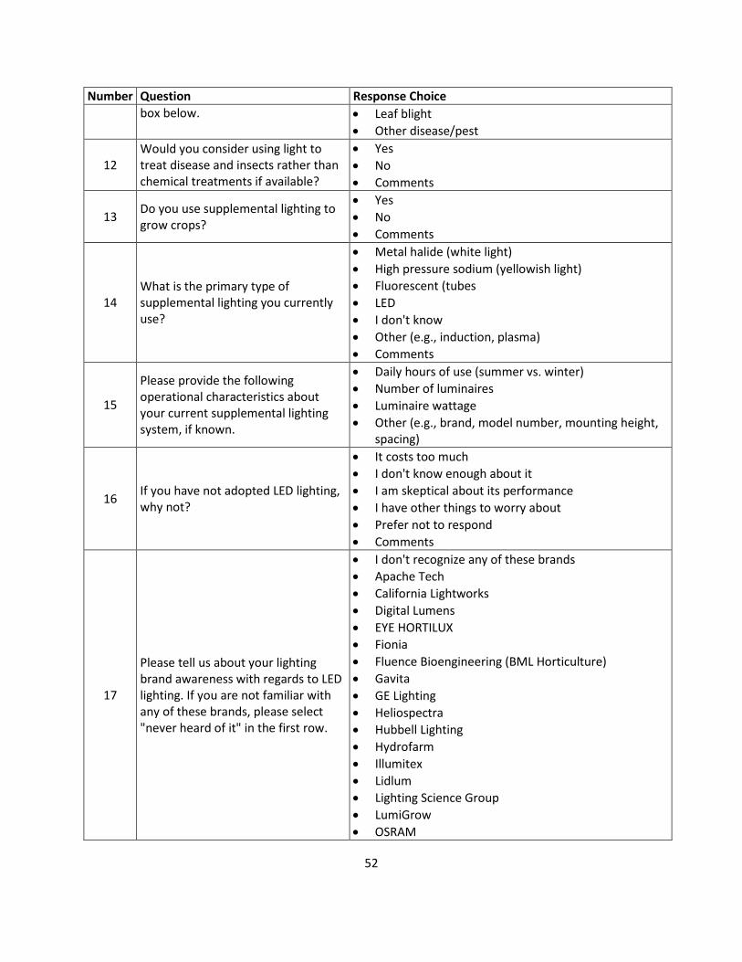
52
Number Question Response Choice box below. • Leaf blight
• Other disease/pest
12 Would you consider using light to treat disease and insects rather than chemical treatments if available?
• Yes • No • Comments
13 Do you use supplemental lighting to grow crops?
• Yes • No • Comments
14 What is the primary type of supplemental lighting you currently use?
• Metal halide (white light) • High pressure sodium (yellowish light) • Fluorescent (tubes • LED • I don't know • Other (e.g., induction, plasma) • Comments
15
Please provide the following operational characteristics about your current supplemental lighting system, if known.
• Daily hours of use (summer vs. winter) • Number of luminaires • Luminaire wattage • Other (e.g., brand, model number, mounting height,
spacing)
16 If you have not adopted LED lighting, why not?
• It costs too much • I don't know enough about it • I am skeptical about its performance • I have other things to worry about • Prefer not to respond • Comments
17
Please tell us about your lighting brand awareness with regards to LED lighting. If you are not familiar with any of these brands, please select "never heard of it" in the first row.
• I don't recognize any of these brands • Apache Tech • California Lightworks • Digital Lumens • EYE HORTILUX • Fionia • Fluence Bioengineering (BML Horticulture) • Gavita • GE Lighting • Heliospectra • Hubbell Lighting • Hydrofarm • Illumitex • Lidlum • Lighting Science Group • LumiGrow • OSRAM

53
Number Question Response Choice • Philips Lighting• PL Light Systems• Sunlight Supply• Valoya• Comments
18
If you have direct experience with LED lighting for horticulture and would like to share information about an installation (e.g., spectral tuning), please provide comments below and, optionally, your contact information.
Open-ended response
19
Thank you for your time and attention. If you have additional comments, please let us know in the comment box below. The link below will include survey results in the near future.
Open-ended response

54
Appendix B: Data sheets The Framework section describes each of the metrics used in the data sheets.

Gavita - Pro 1000e DE US 120-2401000 W HPS Grow Light
Voltage = 240 V. PF = 0.99. PPF (Φp)1 = 1837 µmol s-1 Φp%2 = 76.7 %
Power = 1069 W. THD = 7.5%. PPF/W (Kp) = 1.7 µmol J-1. PSS3 = 0.84
Luminaire System Application Efficacy (LSAE, µmol J-1)4MountHeight(MH)
75 PPFDµmol m-2 s-1
150 PPFDµmol m-2 s-1
225 PPFDµmol m-2 s-1
300 PPFDµmol m-2 s-1
500 PPFDµmol m-2 s-1
1000 PPFDµmol m-2 s-1
ft (m) LSAE QTY LSAE QTY LSAE QTY LSAE QTY LSAE QTY LSAE QTY1 (0.3) 0.37* 8 0.40* 12 0.39* 15 0.44* 20 0.61* 36 0.79* 63
2 (0.6) 0.96* 9 0.80* 12 0.84* 16 1.28* 24 1.26* 35 1.36* 72
3 (0.9) 1.35* 9 1.13* 12 1.32* 20 1.31* 24 1.30* 40 1.28* 77
4 (1.2) 1.28* 9 1.27* 15 1.25* 21 1.21* 24 1.21* 42 1.17* 78
5 (1.5) 1.23* 10 1.17* 15 1.15* 21 1.14* 28 1.12* 45 1.10* 85
6 (1.8) 1.14* 10 1.09* 16 1.08* 24 1.05* 28 1.02* 44 1.03* 92
7 (2.1) 1.06* 10 1.03* 18 1.01* 24 0.97* 28 1.00* 52 0.99* 100
8 (2.4) 0.99* 10 0.96* 18 0.93* 24 0.90* 30 0.93* 54 0.92* 105
Note- LSAE is for a 30ft (9.1m) x 36ft (10.9m) (1080ft2[100.3m2]) growing area with a target min:average uniformity >= 0.6.Bolded text- Highest LSAE for all mounting heights and PPFD combinations.Underlined text- Highest LSAE for target PPFD.* - Combination could not meet target uniformity (min:average >= 0.6), the best uniformity of the tested arrangements was chosen.Gray shaded cells- No layout for this mounting height could meet the target PPFD. The maximum number of luminaires that could fit in the growing area (n=1804) was used instead.
Spectral Power Distribution5
Photosynthetic Photon Flux (Φp) Comparison6
Photosynthetic Photon Flux Efficacy (Kp) Comparison7
Life Cycle Cost Analysis (LCCA)8Summary(Assuming target PPFD of300 µmol m-2 s-1)
Units 1000 W
HPS9600 W
HPS10This HPS11
Quantity 25. 50. 24.
Luminaire Cost US$ 525. 460. 540.
Initial Install Cost US$ 14,850. 26,450. 14,616.
Initial Install Costper Area
US$/ft2
(US$/m2 )
14.
(148).24.
(264).14.
(146).
Lighting Power Density W/ft2
(W/m2 )24.
(263).32.
(344).24.
(256).
Annual EnergyUse per Area
kWh/ft2 yr(kWh/m2 yr)
73.
(790).96.
(1,032).71.
(767).
$.10/kWh 7.69.
(82.83).10.04.
(108.11).7.47.
(80.42).Annual EnergyCost per Area
$.20/kWh
US$/ft2 yr(US$/m2 yr) 14.68.
(158.07).10.04.
(108.11).14.26.
(153.46).
$.10/kWh % <0.0% - No Payback within 20 years..Rate of Returnvs 1000 W HPS $.20/kWh % <0.0% - No Payback within 20 years..
$.10/kWh % 13.3% - Payback at year 1..Rate of Returnvs 600 W HPS $.20/kWh % 30.6% - Payback at year 1..
$.10/kWh 173,081. 238,972. 198,503.Total Payments20 years $.20/kWh
US$(Present Worth) 285,374. 385,538. 307,528.
.Note: Luminaires are used for 3000 hours per year.Note: All calculations assume a 30ft (9.1m) x 36ft (10.9m) (1080ft2[100.3m2]) growing area.
Estimated Cumulative CostsOver 20 Years At $0.10/kWh12
Estimated Cumulative CostsOver 20 Years At $0.20/kWh13
LRC Horticultural Metrics1 of 2
Generated: 2018-03-22
55
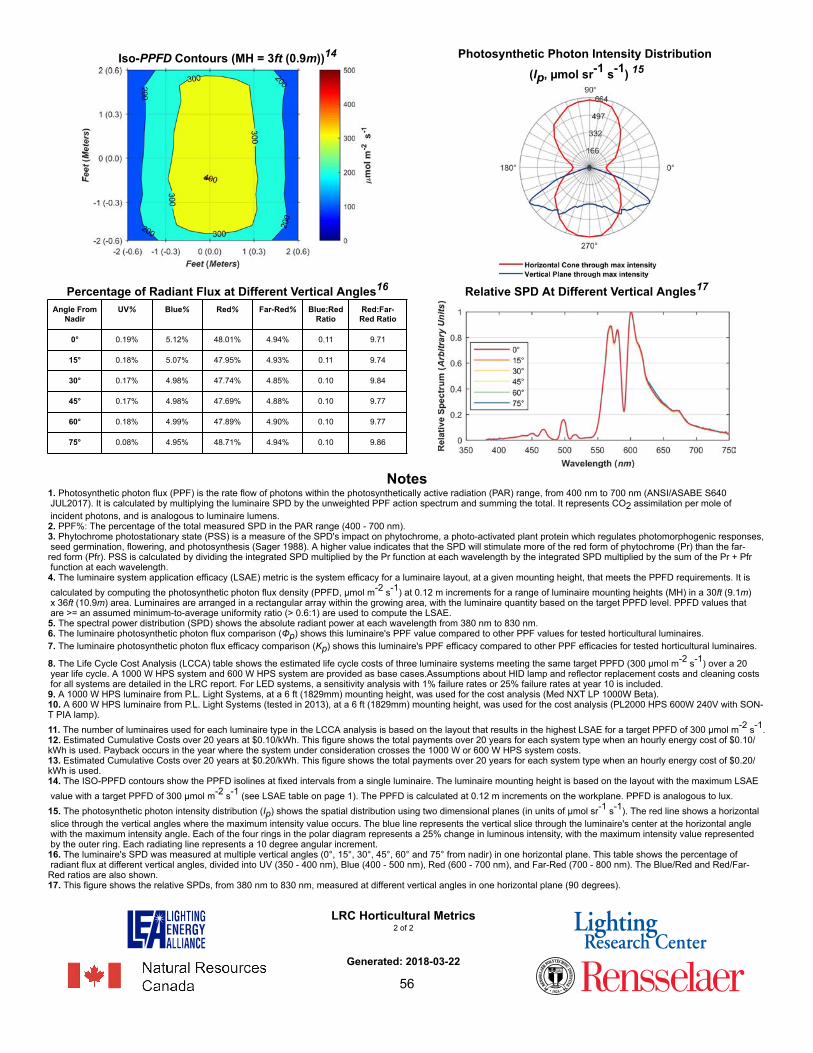
Iso-PPFD Contours (MH = 3ft (0.9m))14 Photosynthetic Photon Intensity Distribution (Ip, µmol sr-1 s-1) 15
Percentage of Radiant Flux at Different Vertical Angles16
Angle FromNadir
UV% Blue% Red% Far-Red% Blue:RedRatio
Red:Far-Red Ratio
0° 0.19% 5.12% 48.01% 4.94% 0.11 9.71
15° 0.18% 5.07% 47.95% 4.93% 0.11 9.74
30° 0.17% 4.98% 47.74% 4.85% 0.10 9.84
45° 0.17% 4.98% 47.69% 4.88% 0.10 9.77
60° 0.18% 4.99% 47.89% 4.90% 0.10 9.77
75° 0.08% 4.95% 48.71% 4.94% 0.10 9.86
Relative SPD At Different Vertical Angles17
Notes1. Photosynthetic photon flux (PPF) is the rate flow of photons within the photosynthetically active radiation (PAR) range, from 400 nm to 700 nm (ANSI/ASABE S640 JUL2017). It is calculated by multiplying the luminaire SPD by the unweighted PPF action spectrum and summing the total. It represents CO2 assimilation per mole of incident photons, and is analogous to luminaire lumens.2. PPF%: The percentage of the total measured SPD in the PAR range (400 - 700 nm).3. Phytochrome photostationary state (PSS) is a measure of the SPD's impact on phytochrome, a photo-activated plant protein which regulates photomorphogenic responses, seed germination, flowering, and photosynthesis (Sager 1988). A higher value indicates that the SPD will stimulate more of the red form of phytochrome (Pr) than the far-red form (Pfr). PSS is calculated by dividing the integrated SPD multiplied by the Pr function at each wavelength by the integrated SPD multiplied by the sum of the Pr + Pfr function at each wavelength.4. The luminaire system application efficacy (LSAE) metric is the system efficacy for a luminaire layout, at a given mounting height, that meets the PPFD requirements. It is calculated by computing the photosynthetic photon flux density (PPFD, µmol m-2 s-1) at 0.12 m increments for a range of luminaire mounting heights (MH) in a 30ft (9.1m) x 36ft (10.9m) area. Luminaires are arranged in a rectangular array within the growing area, with the luminaire quantity based on the target PPFD level. PPFD values that are >= an assumed minimum-to-average uniformity ratio (> 0.6:1) are used to compute the LSAE.5. The spectral power distribution (SPD) shows the absolute radiant power at each wavelength from 380 nm to 830 nm.6. The luminaire photosynthetic photon flux comparison (Φp) shows this luminaire's PPF value compared to other PPF values for tested horticultural luminaires.7. The luminaire photosynthetic photon flux efficacy comparison (Kp) shows this luminaire's PPF efficacy compared to other PPF efficacies for tested horticultural luminaires.
8. The Life Cycle Cost Analysis (LCCA) table shows the estimated life cycle costs of three luminaire systems meeting the same target PPFD (300 µmol m-2 s-1) over a 20 year life cycle. A 1000 W HPS system and 600 W HPS system are provided as base cases.Assumptions about HID lamp and reflector replacement costs and cleaning costs for all systems are detailed in the LRC report. For LED systems, a sensitivity analysis with 1% failure rates or 25% failure rates at year 10 is included.9. A 1000 W HPS luminaire from P.L. Light Systems, at a 6 ft (1829mm) mounting height, was used for the cost analysis (Med NXT LP 1000W Beta).10. A 600 W HPS luminaire from P.L. Light Systems (tested in 2013), at a 6 ft (1829mm) mounting height, was used for the cost analysis (PL2000 HPS 600W 240V with SON-T PIA lamp).11. The number of luminaires used for each luminaire type in the LCCA analysis is based on the layout that results in the highest LSAE for a target PPFD of 300 µmol m-2 s-1.12. Estimated Cumulative Costs over 20 years at $0.10/kWh. This figure shows the total payments over 20 years for each system type when an hourly energy cost of $0.10/kWh is used. Payback occurs in the year where the system under consideration crosses the 1000 W or 600 W HPS system costs.13. Estimated Cumulative Costs over 20 years at $0.20/kWh. This figure shows the total payments over 20 years for each system type when an hourly energy cost of $0.20/kWh is used.14. The ISO-PPFD contours show the PPFD isolines at fixed intervals from a single luminaire. The luminaire mounting height is based on the layout with the maximum LSAE value with a target PPFD of 300 µmol m-2 s-1 (see LSAE table on page 1). The PPFD is calculated at 0.12 m increments on the workplane. PPFD is analogous to lux.15. The photosynthetic photon intensity distribution (Ip) shows the spatial distribution using two dimensional planes (in units of µmol sr-1 s-1). The red line shows a horizontal slice through the vertical angles where the maximum intensity value occurs. The blue line represents the vertical slice through the luminaire's center at the horizontal angle with the maximum intensity angle. Each of the four rings in the polar diagram represents a 25% change in luminous intensity, with the maximum intensity value represented by the outer ring. Each radiating line represents a 10 degree angular increment.16. The luminaire's SPD was measured at multiple vertical angles (0°, 15°, 30°, 45°, 60° and 75° from nadir) in one horizontal plane. This table shows the percentage of radiant flux at different vertical angles, divided into UV (350 - 400 nm), Blue (400 - 500 nm), Red (600 - 700 nm), and Far-Red (700 - 800 nm). The Blue/Red and Red/Far-Red ratios are also shown.17. This figure shows the relative SPDs, from 380 nm to 830 nm, measured at different vertical angles in one horizontal plane (90 degrees).
LRC Horticultural Metrics2 of 2
Generated: 2018-03-22
56

P.L. Light Systems - Med NXT LP 1000W Beta1000 W HPS with Beta reflector
Voltage = 240 V. PF = 0.98. PPF (Φp)1 = 1801 µmol s-1 Φp%2 = 77.2 %
Power = 1057 W. THD = 5.4%. PPF/W (Kp) = 1.7 µmol J-1. PSS3 = 0.85
Luminaire System Application Efficacy (LSAE, µmol J-1)4MountHeight(MH)
75 PPFDµmol m-2 s-1
150 PPFDµmol m-2 s-1
225 PPFDµmol m-2 s-1
300 PPFDµmol m-2 s-1
500 PPFDµmol m-2 s-1
1000 PPFDµmol m-2 s-1
ft (m) LSAE QTY LSAE QTY LSAE QTY LSAE QTY LSAE QTY LSAE QTY1 (0.3) 0.27* 8 0.31* 12 0.41* 18 0.41* 21 0.56* 36 0.61* 66
2 (0.6) 0.74* 9 0.70* 12 0.91* 18 1.02* 24 1.28* 36 1.32* 70
3 (0.9) 1.18* 9 1.20* 12 1.26* 18 1.27* 24 1.33* 40 1.31* 72
4 (1.2) 1.30* 9 1.32* 15 1.30* 20 1.26* 24 1.26* 42 1.22* 77
5 (1.5) 1.29* 10 1.23* 15 1.21* 20 1.19* 25 1.17* 42 1.16* 84
6 (1.8) 1.22* 9 1.17* 16 1.14* 20 1.10* 25 1.10* 45 1.08* 85
7 (2.1) 1.15* 9 1.10* 16 1.08* 24 1.04* 28 1.02* 44 1.03* 92
8 (2.4) 1.07* 9 1.02* 16 1.01* 24 1.01* 32 0.97* 48 0.97* 96
Note- LSAE is for a 30ft (9.1m) x 36ft (10.9m) (1080ft2[100.3m2]) growing area with a target min:average uniformity >= 0.6.Bolded text- Highest LSAE for all mounting heights and PPFD combinations.Underlined text- Highest LSAE for target PPFD.* - Combination could not meet target uniformity (min:average >= 0.6), the best uniformity of the tested arrangements was chosen.Gray shaded cells- No layout for this mounting height could meet the target PPFD. The maximum number of luminaires that could fit in the growing area (n=1890) was used instead.
Spectral Power Distribution5
Photosynthetic Photon Flux (Φp) Comparison6
Photosynthetic Photon Flux Efficacy (Kp) Comparison7
Life Cycle Cost Analysis (LCCA)8Summary(Assuming target PPFD of300 µmol m-2 s-1)
Units 1000 W
HPS9600 W
HPS10This HPS11
Quantity 25. 50. 24.
Luminaire Cost US$ 525. 460. 525.
Initial Install Cost US$ 14,850. 26,450. 14,256.
Initial Install Costper Area
US$/ft2
(US$/m2 )
14.
(148).24.
(264).13.
(142).
Lighting Power Density W/ft2
(W/m2 )24.
(263).32.
(344).23.
(253).
Annual EnergyUse per Area
kWh/ft2 yr(kWh/m2 yr)
73.
(790).96.
(1,032).70.
(759).
$.10/kWh 7.69.
(82.83).10.04.
(108.11).7.39.
(79.51).Annual EnergyCost per Area
$.20/kWh
US$/ft2 yr(US$/m2 yr) 14.68.
(158.07).10.04.
(108.11).14.10.
(151.74).
$.10/kWh % 2.5% - Payback at year 1..Rate of Returnvs 1000 W HPS $.20/kWh % 4.7% - Payback at year 1..
$.10/kWh % 28.3% - Payback at year 1..Rate of Returnvs 600 W HPS $.20/kWh % 46.5% - Payback at year 1..
$.10/kWh 173,081. 238,972. 167,128.Total Payments20 years $.20/kWh
US$(Present Worth) 285,374. 385,538. 274,930.
.Note: Luminaires are used for 3000 hours per year.Note: All calculations assume a 30ft (9.1m) x 36ft (10.9m) (1080ft2[100.3m2]) growing area.
Estimated Cumulative CostsOver 20 Years At $0.10/kWh12
Estimated Cumulative CostsOver 20 Years At $0.20/kWh13
LRC Horticultural Metrics1 of 2
Generated: 2018-03-22
57

Iso-PPFD Contours (MH = 3ft (0.9m))14 Photosynthetic Photon Intensity Distribution (Ip, µmol sr-1 s-1) 15
Percentage of Radiant Flux at Different Vertical Angles16
Angle FromNadir
UV% Blue% Red% Far-Red% Blue:RedRatio
Red:Far-Red Ratio
0° 0.20% 5.26% 44.22% 4.15% 0.12 10.67
15° 0.21% 5.35% 44.47% 4.20% 0.12 10.58
30° 0.21% 5.35% 44.71% 4.28% 0.12 10.45
45° 0.20% 5.24% 44.71% 4.29% 0.12 10.41
60° 0.18% 5.17% 45.07% 4.32% 0.11 10.43
75° 0.10% 5.14% 46.15% 4.33% 0.11 10.65
Relative SPD At Different Vertical Angles17
Notes1. Photosynthetic photon flux (PPF) is the rate flow of photons within the photosynthetically active radiation (PAR) range, from 400 nm to 700 nm (ANSI/ASABE S640 JUL2017). It is calculated by multiplying the luminaire SPD by the unweighted PPF action spectrum and summing the total. It represents CO2 assimilation per mole of incident photons, and is analogous to luminaire lumens.2. PPF%: The percentage of the total measured SPD in the PAR range (400 - 700 nm).3. Phytochrome photostationary state (PSS) is a measure of the SPD's impact on phytochrome, a photo-activated plant protein which regulates photomorphogenic responses, seed germination, flowering, and photosynthesis (Sager 1988). A higher value indicates that the SPD will stimulate more of the red form of phytochrome (Pr) than the far-red form (Pfr). PSS is calculated by dividing the integrated SPD multiplied by the Pr function at each wavelength by the integrated SPD multiplied by the sum of the Pr + Pfr function at each wavelength.4. The luminaire system application efficacy (LSAE) metric is the system efficacy for a luminaire layout, at a given mounting height, that meets the PPFD requirements. It is calculated by computing the photosynthetic photon flux density (PPFD, µmol m-2 s-1) at 0.12 m increments for a range of luminaire mounting heights (MH) in a 30ft (9.1m) x 36ft (10.9m) area. Luminaires are arranged in a rectangular array within the growing area, with the luminaire quantity based on the target PPFD level. PPFD values that are >= an assumed minimum-to-average uniformity ratio (> 0.6:1) are used to compute the LSAE.5. The spectral power distribution (SPD) shows the absolute radiant power at each wavelength from 380 nm to 830 nm.6. The luminaire photosynthetic photon flux comparison (Φp) shows this luminaire's PPF value compared to other PPF values for tested horticultural luminaires.7. The luminaire photosynthetic photon flux efficacy comparison (Kp) shows this luminaire's PPF efficacy compared to other PPF efficacies for tested horticultural luminaires.
8. The Life Cycle Cost Analysis (LCCA) table shows the estimated life cycle costs of three luminaire systems meeting the same target PPFD (300 µmol m-2 s-1) over a 20 year life cycle. A 1000 W HPS system and 600 W HPS system are provided as base cases.Assumptions about HID lamp and reflector replacement costs and cleaning costs for all systems are detailed in the LRC report. For LED systems, a sensitivity analysis with 1% failure rates or 25% failure rates at year 10 is included.9. A 1000 W HPS luminaire from P.L. Light Systems, at a 6 ft (1829mm) mounting height, was used for the cost analysis (Med NXT LP 1000W Beta).10. A 600 W HPS luminaire from P.L. Light Systems (tested in 2013), at a 6 ft (1829mm) mounting height, was used for the cost analysis (PL2000 HPS 600W 240V with SON-T PIA lamp).11. The number of luminaires used for each luminaire type in the LCCA analysis is based on the layout that results in the highest LSAE for a target PPFD of 300 µmol m-2 s-1.12. Estimated Cumulative Costs over 20 years at $0.10/kWh. This figure shows the total payments over 20 years for each system type when an hourly energy cost of $0.10/kWh is used. Payback occurs in the year where the system under consideration crosses the 1000 W or 600 W HPS system costs.13. Estimated Cumulative Costs over 20 years at $0.20/kWh. This figure shows the total payments over 20 years for each system type when an hourly energy cost of $0.20/kWh is used.14. The ISO-PPFD contours show the PPFD isolines at fixed intervals from a single luminaire. The luminaire mounting height is based on the layout with the maximum LSAE value with a target PPFD of 300 µmol m-2 s-1 (see LSAE table on page 1). The PPFD is calculated at 0.12 m increments on the workplane. PPFD is analogous to lux.15. The photosynthetic photon intensity distribution (Ip) shows the spatial distribution using two dimensional planes (in units of µmol sr-1 s-1). The red line shows a horizontal slice through the vertical angles where the maximum intensity value occurs. The blue line represents the vertical slice through the luminaire's center at the horizontal angle with the maximum intensity angle. Each of the four rings in the polar diagram represents a 25% change in luminous intensity, with the maximum intensity value represented by the outer ring. Each radiating line represents a 10 degree angular increment.16. The luminaire's SPD was measured at multiple vertical angles (0°, 15°, 30°, 45°, 60° and 75° from nadir) in one horizontal plane. This table shows the percentage of radiant flux at different vertical angles, divided into UV (350 - 400 nm), Blue (400 - 500 nm), Red (600 - 700 nm), and Far-Red (700 - 800 nm). The Blue/Red and Red/Far-Red ratios are also shown.17. This figure shows the relative SPDs, from 380 nm to 830 nm, measured at different vertical angles in one horizontal plane (90 degrees).
LRC Horticultural Metrics2 of 2
Generated: 2018-03-22
58

P.L. Light Systems - MEDSLA/MH/1000W/277V USH1000 W MH with Maxima reflector
Voltage = 277 V. PF = 0.99. PPF (Φp)1 = 866 µmol s-1 Φp%2 = 84.3 %
Power = 1042 W. THD = 2.6%. PPF/W (Kp) = 0.8 µmol J-1. PSS3 = 0.77
Luminaire System Application Efficacy (LSAE, µmol J-1)4MountHeight(MH)
75 PPFDµmol m-2 s-1
150 PPFDµmol m-2 s-1
225 PPFDµmol m-2 s-1
300 PPFDµmol m-2 s-1
500 PPFDµmol m-2 s-1
1000 PPFDµmol m-2 s-1
ft (m) LSAE QTY LSAE QTY LSAE QTY LSAE QTY LSAE QTY LSAE QTY1 (0.3) 0.19* 12 0.28* 24 0.27* 30 0.32* 42 0.40* 72 0.66* 140
2 (0.6) 0.35* 12 0.60* 25 0.62* 36 0.60* 45 0.60* 72 0.61* 147
3 (0.9) 0.60* 15 0.58* 25 0.58* 36 0.59* 49 0.59* 80 0.58* 160
4 (1.2) 0.58* 16 0.54* 25 0.56* 42 0.55* 54 0.55* 88 0.54* 171
5 (1.5) 0.54* 16 0.53* 30 0.50* 40 0.51* 55 0.50* 91 0.50* 184
6 (1.8) 0.49* 16 0.49* 32 0.49* 48 0.48* 60 0.46* 96 0.47* 198
7 (2.1) 0.45* 16 0.46* 35 0.45* 50 0.45* 65 0.44* 105 0.44* 210
8 (2.4) 0.43* 18 0.42* 35 0.41* 50 0.42* 70 0.42* 115 0.41* 225
Note- LSAE is for a 30ft (9.1m) x 36ft (10.9m) (1080ft2[100.3m2]) growing area with a target min:average uniformity >= 0.6.Bolded text- Highest LSAE for all mounting heights and PPFD combinations.Underlined text- Highest LSAE for target PPFD.* - Combination could not meet target uniformity (min:average >= 0.6), the best uniformity of the tested arrangements was chosen.Gray shaded cells- No layout for this mounting height could meet the target PPFD. The maximum number of luminaires that could fit in the growing area (n=1080) was used instead.
Spectral Power Distribution5
Photosynthetic Photon Flux (Φp) Comparison6
Photosynthetic Photon Flux Efficacy (Kp) Comparison7
Life Cycle Cost Analysis (LCCA)8Summary(Assuming target PPFD of300 µmol m-2 s-1)
Units 1000 W
HPS9600 W
HPS10This MH11
Quantity 25. 50. 45.
Luminaire Cost US$ 525. 460. 569.
Initial Install Cost US$ 14,850. 26,450. 28,710.
Initial Install Costper Area
US$/ft2
(US$/m2 )
14.
(148).24.
(264).27.
(286).
Lighting Power Density W/ft2
(W/m2 )24.
(263).32.
(344).43.
(467).
Annual EnergyUse per Area
kWh/ft2 yr(kWh/m2 yr)
73.
(790).96.
(1,032).130.
(1,402).
$.10/kWh 7.69.
(82.83).10.04.
(108.11).13.65.
(146.96).Annual EnergyCost per Area
$.20/kWh
US$/ft2 yr(US$/m2 yr) 14.68.
(158.07).10.04.
(108.11).26.06.
(280.45).
$.10/kWh % <0.0% - No Payback within 20 years..Rate of Returnvs 1000 W HPS $.20/kWh % <0.0% - No Payback within 20 years..
$.10/kWh % <0.0% - No Payback within 20 years..Rate of Returnvs 600 W HPS $.20/kWh % <0.0% - No Payback within 20 years..
$.10/kWh 173,081. 238,972. 325,603.Total Payments20 years $.20/kWh
US$(Present Worth) 285,374. 385,538. 524,844.
.Note: Luminaires are used for 3000 hours per year.Note: All calculations assume a 30ft (9.1m) x 36ft (10.9m) (1080ft2[100.3m2]) growing area.
Estimated Cumulative CostsOver 20 Years At $0.10/kWh12
Estimated Cumulative CostsOver 20 Years At $0.20/kWh13
LRC Horticultural Metrics1 of 2
Generated: 2018-03-22
59

Iso-PPFD Contours (MH = 2ft (0.6m))14 Photosynthetic Photon Intensity Distribution (Ip, µmol sr-1 s-1) 15
Percentage of Radiant Flux at Different Vertical Angles16
Angle FromNadir
UV% Blue% Red% Far-Red% Blue:RedRatio
Red:Far-Red Ratio
0° 3.00% 38.61% 13.41% 2.54% 2.88 5.29
15° 2.92% 37.95% 13.82% 2.54% 2.75 5.43
30° 2.95% 37.50% 14.06% 2.60% 2.67 5.41
45° 2.95% 36.88% 14.52% 2.67% 2.54 5.43
60° 2.87% 35.90% 15.16% 2.80% 2.37 5.41
75° 2.40% 32.28% 17.42% 3.24% 1.85 5.37
Relative SPD At Different Vertical Angles17
Notes1. Photosynthetic photon flux (PPF) is the rate flow of photons within the photosynthetically active radiation (PAR) range, from 400 nm to 700 nm (ANSI/ASABE S640 JUL2017). It is calculated by multiplying the luminaire SPD by the unweighted PPF action spectrum and summing the total. It represents CO2 assimilation per mole of incident photons, and is analogous to luminaire lumens.2. PPF%: The percentage of the total measured SPD in the PAR range (400 - 700 nm).3. Phytochrome photostationary state (PSS) is a measure of the SPD's impact on phytochrome, a photo-activated plant protein which regulates photomorphogenic responses, seed germination, flowering, and photosynthesis (Sager 1988). A higher value indicates that the SPD will stimulate more of the red form of phytochrome (Pr) than the far-red form (Pfr). PSS is calculated by dividing the integrated SPD multiplied by the Pr function at each wavelength by the integrated SPD multiplied by the sum of the Pr + Pfr function at each wavelength.4. The luminaire system application efficacy (LSAE) metric is the system efficacy for a luminaire layout, at a given mounting height, that meets the PPFD requirements. It is calculated by computing the photosynthetic photon flux density (PPFD, µmol m-2 s-1) at 0.12 m increments for a range of luminaire mounting heights (MH) in a 30ft (9.1m) x 36ft (10.9m) area. Luminaires are arranged in a rectangular array within the growing area, with the luminaire quantity based on the target PPFD level. PPFD values that are >= an assumed minimum-to-average uniformity ratio (> 0.6:1) are used to compute the LSAE.5. The spectral power distribution (SPD) shows the absolute radiant power at each wavelength from 380 nm to 830 nm.6. The luminaire photosynthetic photon flux comparison (Φp) shows this luminaire's PPF value compared to other PPF values for tested horticultural luminaires.7. The luminaire photosynthetic photon flux efficacy comparison (Kp) shows this luminaire's PPF efficacy compared to other PPF efficacies for tested horticultural luminaires.
8. The Life Cycle Cost Analysis (LCCA) table shows the estimated life cycle costs of three luminaire systems meeting the same target PPFD (300 µmol m-2 s-1) over a 20 year life cycle. A 1000 W HPS system and 600 W HPS system are provided as base cases.Assumptions about HID lamp and reflector replacement costs and cleaning costs for all systems are detailed in the LRC report. For LED systems, a sensitivity analysis with 1% failure rates or 25% failure rates at year 10 is included.9. A 1000 W HPS luminaire from P.L. Light Systems, at a 6 ft (1829mm) mounting height, was used for the cost analysis (Med NXT LP 1000W Beta).10. A 600 W HPS luminaire from P.L. Light Systems (tested in 2013), at a 6 ft (1829mm) mounting height, was used for the cost analysis (PL2000 HPS 600W 240V with SON-T PIA lamp).11. The number of luminaires used for each luminaire type in the LCCA analysis is based on the layout that results in the highest LSAE for a target PPFD of 300 µmol m-2 s-1.12. Estimated Cumulative Costs over 20 years at $0.10/kWh. This figure shows the total payments over 20 years for each system type when an hourly energy cost of $0.10/kWh is used. Payback occurs in the year where the system under consideration crosses the 1000 W or 600 W HPS system costs.13. Estimated Cumulative Costs over 20 years at $0.20/kWh. This figure shows the total payments over 20 years for each system type when an hourly energy cost of $0.20/kWh is used.14. The ISO-PPFD contours show the PPFD isolines at fixed intervals from a single luminaire. The luminaire mounting height is based on the layout with the maximum LSAE value with a target PPFD of 300 µmol m-2 s-1 (see LSAE table on page 1). The PPFD is calculated at 0.12 m increments on the workplane. PPFD is analogous to lux.15. The photosynthetic photon intensity distribution (Ip) shows the spatial distribution using two dimensional planes (in units of µmol sr-1 s-1). The red line shows a horizontal slice through the vertical angles where the maximum intensity value occurs. The blue line represents the vertical slice through the luminaire's center at the horizontal angle with the maximum intensity angle. Each of the four rings in the polar diagram represents a 25% change in luminous intensity, with the maximum intensity value represented by the outer ring. Each radiating line represents a 10 degree angular increment.16. The luminaire's SPD was measured at multiple vertical angles (0°, 15°, 30°, 45°, 60° and 75° from nadir) in one horizontal plane. This table shows the percentage of radiant flux at different vertical angles, divided into UV (350 - 400 nm), Blue (400 - 500 nm), Red (600 - 700 nm), and Far-Red (700 - 800 nm). The Blue/Red and Red/Far-Red ratios are also shown.17. This figure shows the relative SPDs, from 380 nm to 830 nm, measured at different vertical angles in one horizontal plane (90 degrees).
LRC Horticultural Metrics2 of 2
Generated: 2018-03-22
60

GE Lighting - GEHL48HPKB1Arize Lynk
Voltage = 120 V. PF = 0.99. PPF (Φp)1 = 79 µmol s-1 Φp%2 = 99.9 %
Power = 30 W. THD = 11.5%. PPF/W (Kp) = 2.6 µmol J-1. PSS3 = 0.88
Luminaire System Application Efficacy (LSAE, µmol J-1)4MountHeight(MH)
75 PPFDµmol m-2 s-1
150 PPFDµmol m-2 s-1
225 PPFDµmol m-2 s-1
300 PPFDµmol m-2 s-1
500 PPFDµmol m-2 s-1
1000 PPFDµmol m-2 s-1
ft (m) LSAE QTY LSAE QTY LSAE QTY LSAE QTY LSAE QTY LSAE QTY1 (0.3) 1.04* 144 0.52* 162 0.23* 162 0.07* 162 0.00* 162 0.00* 162
2 (0.6) 1.59* 150 0.21* 162 0.00* 162 0.00* 162 0.00* 162 0.00* 162
3 (0.9) 1.50* 156 0.09* 162 0.00* 162 0.00* 162 0.00* 162 0.00* 162
4 (1.2) 1.45* 162 0.07* 162 0.00* 162 0.00* 162 0.00* 162 0.00* 162
5 (1.5) 1.37* 162 0.00* 162 0.00* 162 0.00* 162 0.00* 162 0.00* 162
6 (1.8) 1.25* 162 0.00* 162 0.00* 162 0.00* 162 0.00* 162 0.00* 162
7 (2.1) 1.14* 162 0.00* 162 0.00* 162 0.00* 162 0.00* 162 0.00* 162
8 (2.4) 1.03* 162 0.00* 162 0.00* 162 0.00* 162 0.00* 162 0.00* 162
Note- LSAE is for a 30ft (9.1m) x 36ft (10.9m) (1080ft2[100.3m2]) growing area with a target min:average uniformity >= 0.6.Bolded text- Highest LSAE for all mounting heights and PPFD combinations.Underlined text- Highest LSAE for target PPFD.* - Combination could not meet target uniformity (min:average >= 0.6), the best uniformity of the tested arrangements was chosen.Gray shaded cells- No layout for this mounting height could meet the target PPFD. The maximum number of luminaires that could fit in the growing area (n=162) was used instead.
Spectral Power Distribution5
Photosynthetic Photon Flux (Φp) Comparison6
Photosynthetic Photon Flux Efficacy (Kp) Comparison7
Life Cycle Cost Analysis (LCCA)8Summary(Assuming target PPFD of75 µmol m-2 s-1)
Units 1000 W
HPS9600 W
HPS10This LED11
Quantity 9. 15. 150.
Luminaire Cost US$ 525. 460. 245.
Initial Install Cost US$ 5,346. 7,935. 47,100.
Initial Install Costper Area
US$/ft2
(US$/m2 )
5.
(53).7.
(79).44.
(469).
Lighting Power Density W/ft2
(W/m2 )9.
(95).10.
(103).4.
(45).
Annual EnergyUse per Area
kWh/ft2 yr(kWh/m2 yr)
26.
(285).29.
(309).12.
(135).
$.10/kWh 2.77.
(29.82).3.01.
(32.43).1.31.
(14.10).Annual EnergyCost per Area
$.20/kWh
US$/ft2 yr(US$/m2 yr) 5.29.
(56.90).3.01.
(32.43).2.50.
(26.91).
$.10/kWh % 3.2% - No Payback within 20 years..Rate of Returnvs 1000 W HPS $.20/kWh % 6.3% - Payback at year 20..
$.10/kWh % 4.2% - No Payback within 20 years..Rate of Returnvs 600 W HPS $.20/kWh % 7.7% - Payback at year 14..
$.10/kWh 62,309. 71,691. 81,806.Total Payments20 years $.20/kWh
US$(Present Worth) 102,735. 115,661. 100,923.
.Note: Luminaires are used for 3000 hours per year.Note: All calculations assume a 30ft (9.1m) x 36ft (10.9m) (1080ft2[100.3m2]) growing area.
Estimated Cumulative CostsOver 20 Years At $0.10/kWh12
Estimated Cumulative CostsOver 20 Years At $0.20/kWh13
LRC Horticultural Metrics1 of 2
Generated: 2018-03-22
61

Iso-PPFD Contours (MH = 1ft (0.3m))14 Photosynthetic Photon Intensity Distribution (Ip, µmol sr-1 s-1) 15
Percentage of Radiant Flux at Different Vertical Angles16
Angle FromNadir
UV% Blue% Red% Far-Red% Blue:RedRatio
Red:Far-Red Ratio
0° 0.05% 30.98% 67.76% 0.19% 0.46 347.63
15° 0.05% 29.47% 69.28% 0.20% 0.43 355.15
30° 0.05% 27.76% 70.94% 0.20% 0.39 350.46
45° 0.05% 25.13% 73.61% 0.19% 0.34 378.31
60° 0.05% 26.37% 70.93% 0.25% 0.37 286.09
75° 0.06% 31.75% 63.51% 0.36% 0.50 178.77
Relative SPD At Different Vertical Angles17
Notes1. Photosynthetic photon flux (PPF) is the rate flow of photons within the photosynthetically active radiation (PAR) range, from 400 nm to 700 nm (ANSI/ASABE S640 JUL2017). It is calculated by multiplying the luminaire SPD by the unweighted PPF action spectrum and summing the total. It represents CO2 assimilation per mole of incident photons, and is analogous to luminaire lumens.2. PPF%: The percentage of the total measured SPD in the PAR range (400 - 700 nm).3. Phytochrome photostationary state (PSS) is a measure of the SPD's impact on phytochrome, a photo-activated plant protein which regulates photomorphogenic responses, seed germination, flowering, and photosynthesis (Sager 1988). A higher value indicates that the SPD will stimulate more of the red form of phytochrome (Pr) than the far-red form (Pfr). PSS is calculated by dividing the integrated SPD multiplied by the Pr function at each wavelength by the integrated SPD multiplied by the sum of the Pr + Pfr function at each wavelength.4. The luminaire system application efficacy (LSAE) metric is the system efficacy for a luminaire layout, at a given mounting height, that meets the PPFD requirements. It is calculated by computing the photosynthetic photon flux density (PPFD, µmol m-2 s-1) at 0.12 m increments for a range of luminaire mounting heights (MH) in a 30ft (9.1m) x 36ft (10.9m) area. Luminaires are arranged in a rectangular array within the growing area, with the luminaire quantity based on the target PPFD level. PPFD values that are >= an assumed minimum-to-average uniformity ratio (> 0.6:1) are used to compute the LSAE.5. The spectral power distribution (SPD) shows the absolute radiant power at each wavelength from 380 nm to 830 nm.6. The luminaire photosynthetic photon flux comparison (Φp) shows this luminaire's PPF value compared to other PPF values for tested horticultural luminaires.7. The luminaire photosynthetic photon flux efficacy comparison (Kp) shows this luminaire's PPF efficacy compared to other PPF efficacies for tested horticultural luminaires.
8. The Life Cycle Cost Analysis (LCCA) table shows the estimated life cycle costs of three luminaire systems meeting the same target PPFD (75 µmol m-2 s-1) over a 20 year life cycle. A 1000 W HPS system and 600 W HPS system are provided as base cases.Assumptions about HID lamp and reflector replacement costs and cleaning costs for all systems are detailed in the LRC report. For LED systems, a sensitivity analysis with 1% failure rates or 25% failure rates at year 10 is included.9. A 1000 W HPS luminaire from P.L. Light Systems, at a 6 ft (1829mm) mounting height, was used for the cost analysis (Med NXT LP 1000W Beta).10. A 600 W HPS luminaire from P.L. Light Systems (tested in 2013), at a 6 ft (1829mm) mounting height, was used for the cost analysis (PL2000 HPS 600W 240V with SON-T PIA lamp).11. The number of luminaires used for each luminaire type in the LCCA analysis is based on the layout that results in the highest LSAE for a target PPFD of 75 µmol m-2 s-1.12. Estimated Cumulative Costs over 20 years at $0.10/kWh. This figure shows the total payments over 20 years for each system type when an hourly energy cost of $0.10/kWh is used. Payback occurs in the year where the system under consideration crosses the 1000 W or 600 W HPS system costs.13. Estimated Cumulative Costs over 20 years at $0.20/kWh. This figure shows the total payments over 20 years for each system type when an hourly energy cost of $0.20/kWh is used.14. The ISO-PPFD contours show the PPFD isolines at fixed intervals from a single luminaire. The luminaire mounting height is based on the layout with the maximum LSAE value with a target PPFD of 300 µmol m-2 s-1 (see LSAE table on page 1). The PPFD is calculated at 0.12 m increments on the workplane. PPFD is analogous to lux.15. The photosynthetic photon intensity distribution (Ip) shows the spatial distribution using two dimensional planes (in units of µmol sr-1 s-1). The red line shows a horizontal slice through the vertical angles where the maximum intensity value occurs. The blue line represents the vertical slice through the luminaire's center at the horizontal angle with the maximum intensity angle. Each of the four rings in the polar diagram represents a 25% change in luminous intensity, with the maximum intensity value represented by the outer ring. Each radiating line represents a 10 degree angular increment.16. The luminaire's SPD was measured at multiple vertical angles (0°, 15°, 30°, 45°, 60° and 75° from nadir) in one horizontal plane. This table shows the percentage of radiant flux at different vertical angles, divided into UV (350 - 400 nm), Blue (400 - 500 nm), Red (600 - 700 nm), and Far-Red (700 - 800 nm). The Blue/Red and Red/Far-Red ratios are also shown.17. This figure shows the relative SPDs, from 380 nm to 830 nm, measured at different vertical angles in one horizontal plane (90 degrees).
LRC Horticultural Metrics2 of 2
Generated: 2018-03-22
62

Heliospectra - LX601CLX601C
Voltage = 120 V. PF = 0.99. PPF (Φp)1 = 673 µmol s-1 Φp%2 = 82.3 %
Power = 595 W. THD = 7.3%. PPF/W (Kp) = 1.1 µmol J-1. PSS3 = 0.80
Luminaire System Application Efficacy (LSAE, µmol J-1)4MountHeight(MH)
75 PPFDµmol m-2 s-1
150 PPFDµmol m-2 s-1
225 PPFDµmol m-2 s-1
300 PPFDµmol m-2 s-1
500 PPFDµmol m-2 s-1
1000 PPFDµmol m-2 s-1
ft (m) LSAE QTY LSAE QTY LSAE QTY LSAE QTY LSAE QTY LSAE QTY1 (0.3) 0.17* 20 0.25* 36 0.31* 49 0.43* 70 0.68* 110 0.77* 221
2 (0.6) 0.47* 20 0.68* 36 0.75* 56 0.71* 70 0.73* 120 0.71* 231
3 (0.9) 0.74* 20 0.67* 40 0.68* 55 0.67* 75 0.68* 125 0.66* 245
4 (1.2) 0.64* 20 0.65* 40 0.64* 60 0.63* 76 0.62* 128 0.62* 260
5 (1.5) 0.66* 24 0.65* 45 0.62* 60 0.63* 84 0.63* 138 0.58* 275
6 (1.8) 0.56* 21 0.56* 42 0.59* 69 0.62* 86 0.57* 147 0.55* 294
7 (2.1) 0.60* 26 0.58* 46 0.57* 68 0.58* 96 0.52* 154 0.51* 308
8 (2.4) 0.57* 24 0.58* 52 0.56* 76 0.56* 102 0.49* 162 0.49* 330
Note- LSAE is for a 30ft (9.1m) x 36ft (10.9m) (1080ft2[100.3m2]) growing area with a target min:average uniformity >= 0.6.Bolded text- Highest LSAE for all mounting heights and PPFD combinations.Underlined text- Highest LSAE for target PPFD.* - Combination could not meet target uniformity (min:average >= 0.6), the best uniformity of the tested arrangements was chosen.Gray shaded cells- No layout for this mounting height could meet the target PPFD. The maximum number of luminaires that could fit in the growing area (n=1380) was used instead.
Spectral Power Distribution5
Photosynthetic Photon Flux (Φp) Comparison6
Photosynthetic Photon Flux Efficacy (Kp) Comparison7
Life Cycle Cost Analysis (LCCA)8Summary(Assuming target PPFD of300 µmol m-2 s-1)
Units 1000 W
HPS9600 W
HPS10This LED11
Quantity 25. 50. 70.
Luminaire Cost US$ 525. 460. 2400.
Initial Install Cost US$ 14,850. 26,450. 172,830.
Initial Install Costper Area
US$/ft2
(US$/m2 )
14.
(148).24.
(264).160.
(1,723).
Lighting Power Density W/ft2
(W/m2 )24.
(263).32.
(344).39.
(415).
Annual EnergyUse per Area
kWh/ft2 yr(kWh/m2 yr)
73.
(790).96.
(1,032).116.
(1,246).
$.10/kWh 7.69.
(82.83).10.04.
(108.11).12.13.
(130.58).Annual EnergyCost per Area
$.20/kWh
US$/ft2 yr(US$/m2 yr) 14.68.
(158.07).10.04.
(108.11).23.15.
(249.19).
$.10/kWh % <0.0% - No Payback within 20 years..Rate of Returnvs 1000 W HPS $.20/kWh % <0.0% - No Payback within 20 years..
$.10/kWh % 0.4% - No Payback within 20 years..Rate of Returnvs 600 W HPS $.20/kWh % <0.0% - No Payback within 20 years..
$.10/kWh 173,081. 238,972. 375,210.Total Payments20 years $.20/kWh
US$(Present Worth) 285,374. 385,538. 552,241.
.Note: Luminaires are used for 3000 hours per year.Note: All calculations assume a 30ft (9.1m) x 36ft (10.9m) (1080ft2[100.3m2]) growing area.
Estimated Cumulative CostsOver 20 Years At $0.10/kWh12
Estimated Cumulative CostsOver 20 Years At $0.20/kWh13
LRC Horticultural Metrics1 of 2
Generated: 2018-03-22
63

Iso-PPFD Contours (MH = 2ft (0.6m))14 Photosynthetic Photon Intensity Distribution (Ip, µmol sr-1 s-1) 15
Percentage of Radiant Flux at Different Vertical Angles16
Angle FromNadir
UV% Blue% Red% Far-Red% Blue:RedRatio
Red:Far-Red Ratio
0° 0.04% 21.96% 51.30% 14.21% 0.43 3.61
15° 0.04% 21.89% 51.07% 14.43% 0.43 3.54
30° 0.04% 21.40% 50.86% 14.95% 0.42 3.40
45° 0.04% 20.70% 50.06% 16.24% 0.41 3.08
60° 0.04% 21.34% 46.04% 21.32% 0.46 2.16
75° 0.03% 18.11% 50.95% 18.78% 0.36 2.71
Relative SPD At Different Vertical Angles17
Notes1. Photosynthetic photon flux (PPF) is the rate flow of photons within the photosynthetically active radiation (PAR) range, from 400 nm to 700 nm (ANSI/ASABE S640 JUL2017). It is calculated by multiplying the luminaire SPD by the unweighted PPF action spectrum and summing the total. It represents CO2 assimilation per mole of incident photons, and is analogous to luminaire lumens.2. PPF%: The percentage of the total measured SPD in the PAR range (400 - 700 nm).3. Phytochrome photostationary state (PSS) is a measure of the SPD's impact on phytochrome, a photo-activated plant protein which regulates photomorphogenic responses, seed germination, flowering, and photosynthesis (Sager 1988). A higher value indicates that the SPD will stimulate more of the red form of phytochrome (Pr) than the far-red form (Pfr). PSS is calculated by dividing the integrated SPD multiplied by the Pr function at each wavelength by the integrated SPD multiplied by the sum of the Pr + Pfr function at each wavelength.4. The luminaire system application efficacy (LSAE) metric is the system efficacy for a luminaire layout, at a given mounting height, that meets the PPFD requirements. It is calculated by computing the photosynthetic photon flux density (PPFD, µmol m-2 s-1) at 0.12 m increments for a range of luminaire mounting heights (MH) in a 30ft (9.1m) x 36ft (10.9m) area. Luminaires are arranged in a rectangular array within the growing area, with the luminaire quantity based on the target PPFD level. PPFD values that are >= an assumed minimum-to-average uniformity ratio (> 0.6:1) are used to compute the LSAE.5. The spectral power distribution (SPD) shows the absolute radiant power at each wavelength from 380 nm to 830 nm.6. The luminaire photosynthetic photon flux comparison (Φp) shows this luminaire's PPF value compared to other PPF values for tested horticultural luminaires.7. The luminaire photosynthetic photon flux efficacy comparison (Kp) shows this luminaire's PPF efficacy compared to other PPF efficacies for tested horticultural luminaires.
8. The Life Cycle Cost Analysis (LCCA) table shows the estimated life cycle costs of three luminaire systems meeting the same target PPFD (300 µmol m-2 s-1) over a 20 year life cycle. A 1000 W HPS system and 600 W HPS system are provided as base cases.Assumptions about HID lamp and reflector replacement costs and cleaning costs for all systems are detailed in the LRC report. For LED systems, a sensitivity analysis with 1% failure rates or 25% failure rates at year 10 is included.9. A 1000 W HPS luminaire from P.L. Light Systems, at a 6 ft (1829mm) mounting height, was used for the cost analysis (Med NXT LP 1000W Beta).10. A 600 W HPS luminaire from P.L. Light Systems (tested in 2013), at a 6 ft (1829mm) mounting height, was used for the cost analysis (PL2000 HPS 600W 240V with SON-T PIA lamp).11. The number of luminaires used for each luminaire type in the LCCA analysis is based on the layout that results in the highest LSAE for a target PPFD of 300 µmol m-2 s-1.12. Estimated Cumulative Costs over 20 years at $0.10/kWh. This figure shows the total payments over 20 years for each system type when an hourly energy cost of $0.10/kWh is used. Payback occurs in the year where the system under consideration crosses the 1000 W or 600 W HPS system costs.13. Estimated Cumulative Costs over 20 years at $0.20/kWh. This figure shows the total payments over 20 years for each system type when an hourly energy cost of $0.20/kWh is used.14. The ISO-PPFD contours show the PPFD isolines at fixed intervals from a single luminaire. The luminaire mounting height is based on the layout with the maximum LSAE value with a target PPFD of 300 µmol m-2 s-1 (see LSAE table on page 1). The PPFD is calculated at 0.12 m increments on the workplane. PPFD is analogous to lux.15. The photosynthetic photon intensity distribution (Ip) shows the spatial distribution using two dimensional planes (in units of µmol sr-1 s-1). The red line shows a horizontal slice through the vertical angles where the maximum intensity value occurs. The blue line represents the vertical slice through the luminaire's center at the horizontal angle with the maximum intensity angle. Each of the four rings in the polar diagram represents a 25% change in luminous intensity, with the maximum intensity value represented by the outer ring. Each radiating line represents a 10 degree angular increment.16. The luminaire's SPD was measured at multiple vertical angles (0°, 15°, 30°, 45°, 60° and 75° from nadir) in one horizontal plane. This table shows the percentage of radiant flux at different vertical angles, divided into UV (350 - 400 nm), Blue (400 - 500 nm), Red (600 - 700 nm), and Far-Red (700 - 800 nm). The Blue/Red and Red/Far-Red ratios are also shown.17. This figure shows the relative SPDs, from 380 nm to 830 nm, measured at different vertical angles in one horizontal plane (90 degrees).
LRC Horticultural Metrics2 of 2
Generated: 2018-03-22
64
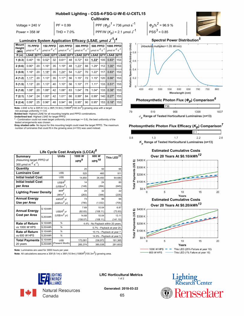
Hubbell Lighting - CGS-4-FSG-U-W-E-U-C6TL15Cultivaire
Voltage = 240 V. PF = 0.99. PPF (Φp)1 = 736 µmol s-1 Φp%2 = 96.9 %
Power = 358 W. THD = 7.0%. PPF/W (Kp) = 2.1 µmol J-1. PSS3 = 0.85
Luminaire System Application Efficacy (LSAE, µmol J-1)4MountHeight(MH)
75 PPFDµmol m-2 s-1
150 PPFDµmol m-2 s-1
225 PPFDµmol m-2 s-1
300 PPFDµmol m-2 s-1
500 PPFDµmol m-2 s-1
1000 PPFDµmol m-2 s-1
ft (m) LSAE QTY LSAE QTY LSAE QTY LSAE QTY LSAE QTY LSAE QTY1 (0.3) 0.40* 18 0.52* 32 0.61* 48 0.72* 63 1.33* 105 0.83* 153
2 (0.6) 0.90* 20 1.16* 35 1.19* 48 1.23* 66 1.29* 112 1.00* 153
3 (0.9) 1.16* 20 1.18* 35 1.24* 54 1.22* 70 1.22* 117 0.83* 153
4 (1.2) 1.17* 20 1.13* 35 1.17* 56 1.15* 72 1.15* 120 0.66* 153
5 (1.5) 1.13* 20 1.13* 40 1.10* 56 1.10* 77 1.11* 133 0.51* 153
6 (1.8) 1.08* 20 1.06* 42 1.06* 63 1.04* 78 1.04* 133 0.38* 153
7 (2.1) 1.04* 24 1.00* 42 1.01* 66 0.99* 84 0.99* 140 0.27* 153
8 (2.4) 0.99* 25 0.96* 48 0.94* 66 0.95* 90 0.95* 153 0.18* 153
Note- LSAE is for a 30ft (9.1m) x 36ft (10.9m) (1080ft2[100.3m2]) growing area with a target min:average uniformity >= 0.6.Bolded text- Highest LSAE for all mounting heights and PPFD combinations.Underlined text- Highest LSAE for target PPFD.* - Combination could not meet target uniformity (min:average >= 0.6), the best uniformity of the tested arrangements was chosen.Gray shaded cells- No layout for this mounting height could meet the target PPFD. The maximum number of luminaires that could fit in the growing area (n=153) was used instead.
Spectral Power Distribution5
Photosynthetic Photon Flux (Φp) Comparison6
Photosynthetic Photon Flux Efficacy (Kp) Comparison7
Life Cycle Cost Analysis (LCCA)8Summary(Assuming target PPFD of300 µmol m-2 s-1)
Units 1000 W
HPS9600 W
HPS10This LED11
Quantity 25. 50. 66.
Luminaire Cost US$ 525. 460. 911.
Initial Install Cost US$ 14,850. 26,450. 64,680.
Initial Install Costper Area
US$/ft2
(US$/m2 )
14.
(148).24.
(264).60.
(645).
Lighting Power Density W/ft2
(W/m2 )24.
(263).32.
(344).22.
(235).
Annual EnergyUse per Area
kWh/ft2 yr(kWh/m2 yr)
73.
(790).96.
(1,032).66.
(705).
$.10/kWh 7.69.
(82.83).10.04.
(108.11).6.87.
(73.93).Annual EnergyCost per Area
$.20/kWh
US$/ft2 yr(US$/m2 yr) 14.68.
(158.07).10.04.
(108.11).13.11.
(141.10).
$.10/kWh % 4.4% - No Payback within 20 years..Rate of Returnvs 1000 W HPS $.20/kWh % 5.7% - Payback at year 20..
$.10/kWh % 10.1% - Payback at year 7..Rate of Returnvs 600 W HPS $.20/kWh % 14.9% - Payback at year 5..
$.10/kWh 173,081. 238,972. 181,365.Total Payments20 years $.20/kWh
US$(Present Worth) 285,374. 385,538. 281,603.
.Note: Luminaires are used for 3000 hours per year.Note: All calculations assume a 30ft (9.1m) x 36ft (10.9m) (1080ft2[100.3m2]) growing area.
Estimated Cumulative CostsOver 20 Years At $0.10/kWh12
Estimated Cumulative CostsOver 20 Years At $0.20/kWh13
LRC Horticultural Metrics1 of 2
Generated: 2018-03-22
65

Iso-PPFD Contours (MH = 2ft (0.6m))14 Photosynthetic Photon Intensity Distribution (Ip, µmol sr-1 s-1) 15
Percentage of Radiant Flux at Different Vertical Angles16
Angle FromNadir
UV% Blue% Red% Far-Red% Blue:RedRatio
Red:Far-Red Ratio
0° 0.02% 20.57% 31.16% 2.66% 0.66 11.71
15° 0.02% 20.74% 31.09% 2.67% 0.67 11.66
30° 0.02% 20.96% 31.01% 2.66% 0.68 11.66
45° 0.02% 21.25% 30.88% 2.66% 0.69 11.62
60° 0.02% 21.52% 30.74% 2.67% 0.70 11.52
75° 0.02% 22.32% 29.89% 2.74% 0.75 10.90
Relative SPD At Different Vertical Angles17
Notes1. Photosynthetic photon flux (PPF) is the rate flow of photons within the photosynthetically active radiation (PAR) range, from 400 nm to 700 nm (ANSI/ASABE S640 JUL2017). It is calculated by multiplying the luminaire SPD by the unweighted PPF action spectrum and summing the total. It represents CO2 assimilation per mole of incident photons, and is analogous to luminaire lumens.2. PPF%: The percentage of the total measured SPD in the PAR range (400 - 700 nm).3. Phytochrome photostationary state (PSS) is a measure of the SPD's impact on phytochrome, a photo-activated plant protein which regulates photomorphogenic responses, seed germination, flowering, and photosynthesis (Sager 1988). A higher value indicates that the SPD will stimulate more of the red form of phytochrome (Pr) than the far-red form (Pfr). PSS is calculated by dividing the integrated SPD multiplied by the Pr function at each wavelength by the integrated SPD multiplied by the sum of the Pr + Pfr function at each wavelength.4. The luminaire system application efficacy (LSAE) metric is the system efficacy for a luminaire layout, at a given mounting height, that meets the PPFD requirements. It is calculated by computing the photosynthetic photon flux density (PPFD, µmol m-2 s-1) at 0.12 m increments for a range of luminaire mounting heights (MH) in a 30ft (9.1m) x 36ft (10.9m) area. Luminaires are arranged in a rectangular array within the growing area, with the luminaire quantity based on the target PPFD level. PPFD values that are >= an assumed minimum-to-average uniformity ratio (> 0.6:1) are used to compute the LSAE.5. The spectral power distribution (SPD) shows the absolute radiant power at each wavelength from 380 nm to 830 nm.6. The luminaire photosynthetic photon flux comparison (Φp) shows this luminaire's PPF value compared to other PPF values for tested horticultural luminaires.7. The luminaire photosynthetic photon flux efficacy comparison (Kp) shows this luminaire's PPF efficacy compared to other PPF efficacies for tested horticultural luminaires.
8. The Life Cycle Cost Analysis (LCCA) table shows the estimated life cycle costs of three luminaire systems meeting the same target PPFD (300 µmol m-2 s-1) over a 20 year life cycle. A 1000 W HPS system and 600 W HPS system are provided as base cases.Assumptions about HID lamp and reflector replacement costs and cleaning costs for all systems are detailed in the LRC report. For LED systems, a sensitivity analysis with 1% failure rates or 25% failure rates at year 10 is included.9. A 1000 W HPS luminaire from P.L. Light Systems, at a 6 ft (1829mm) mounting height, was used for the cost analysis (Med NXT LP 1000W Beta).10. A 600 W HPS luminaire from P.L. Light Systems (tested in 2013), at a 6 ft (1829mm) mounting height, was used for the cost analysis (PL2000 HPS 600W 240V with SON-T PIA lamp).11. The number of luminaires used for each luminaire type in the LCCA analysis is based on the layout that results in the highest LSAE for a target PPFD of 300 µmol m-2 s-1.12. Estimated Cumulative Costs over 20 years at $0.10/kWh. This figure shows the total payments over 20 years for each system type when an hourly energy cost of $0.10/kWh is used. Payback occurs in the year where the system under consideration crosses the 1000 W or 600 W HPS system costs.13. Estimated Cumulative Costs over 20 years at $0.20/kWh. This figure shows the total payments over 20 years for each system type when an hourly energy cost of $0.20/kWh is used.14. The ISO-PPFD contours show the PPFD isolines at fixed intervals from a single luminaire. The luminaire mounting height is based on the layout with the maximum LSAE value with a target PPFD of 300 µmol m-2 s-1 (see LSAE table on page 1). The PPFD is calculated at 0.12 m increments on the workplane. PPFD is analogous to lux.15. The photosynthetic photon intensity distribution (Ip) shows the spatial distribution using two dimensional planes (in units of µmol sr-1 s-1). The red line shows a horizontal slice through the vertical angles where the maximum intensity value occurs. The blue line represents the vertical slice through the luminaire's center at the horizontal angle with the maximum intensity angle. Each of the four rings in the polar diagram represents a 25% change in luminous intensity, with the maximum intensity value represented by the outer ring. Each radiating line represents a 10 degree angular increment.16. The luminaire's SPD was measured at multiple vertical angles (0°, 15°, 30°, 45°, 60° and 75° from nadir) in one horizontal plane. This table shows the percentage of radiant flux at different vertical angles, divided into UV (350 - 400 nm), Blue (400 - 500 nm), Red (600 - 700 nm), and Far-Red (700 - 800 nm). The Blue/Red and Red/Far-Red ratios are also shown.17. This figure shows the relative SPDs, from 380 nm to 830 nm, measured at different vertical angles in one horizontal plane (90 degrees).
LRC Horticultural Metrics2 of 2
Generated: 2018-03-22
66
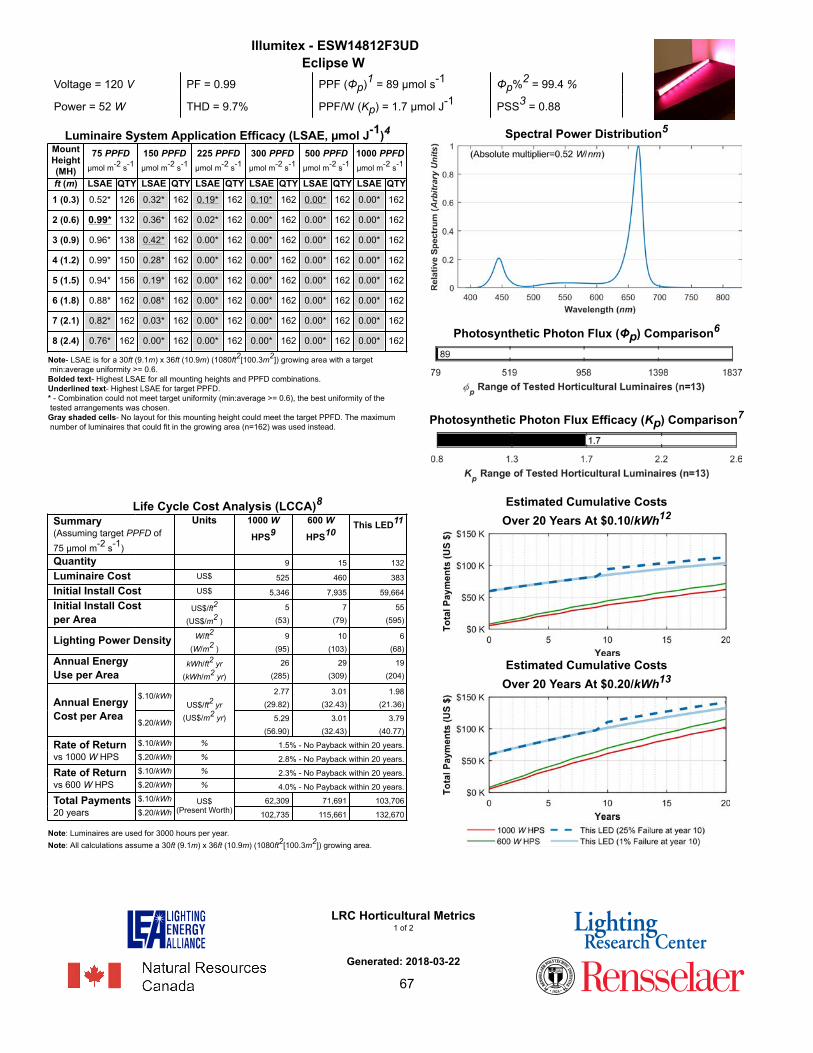
Illumitex - ESW14812F3UDEclipse W
Voltage = 120 V. PF = 0.99. PPF (Φp)1 = 89 µmol s-1 Φp%2 = 99.4 %
Power = 52 W. THD = 9.7%. PPF/W (Kp) = 1.7 µmol J-1. PSS3 = 0.88
Luminaire System Application Efficacy (LSAE, µmol J-1)4MountHeight(MH)
75 PPFDµmol m-2 s-1
150 PPFDµmol m-2 s-1
225 PPFDµmol m-2 s-1
300 PPFDµmol m-2 s-1
500 PPFDµmol m-2 s-1
1000 PPFDµmol m-2 s-1
ft (m) LSAE QTY LSAE QTY LSAE QTY LSAE QTY LSAE QTY LSAE QTY1 (0.3) 0.52* 126 0.32* 162 0.19* 162 0.10* 162 0.00* 162 0.00* 162
2 (0.6) 0.99* 132 0.36* 162 0.02* 162 0.00* 162 0.00* 162 0.00* 162
3 (0.9) 0.96* 138 0.42* 162 0.00* 162 0.00* 162 0.00* 162 0.00* 162
4 (1.2) 0.99* 150 0.28* 162 0.00* 162 0.00* 162 0.00* 162 0.00* 162
5 (1.5) 0.94* 156 0.19* 162 0.00* 162 0.00* 162 0.00* 162 0.00* 162
6 (1.8) 0.88* 162 0.08* 162 0.00* 162 0.00* 162 0.00* 162 0.00* 162
7 (2.1) 0.82* 162 0.03* 162 0.00* 162 0.00* 162 0.00* 162 0.00* 162
8 (2.4) 0.76* 162 0.00* 162 0.00* 162 0.00* 162 0.00* 162 0.00* 162
Note- LSAE is for a 30ft (9.1m) x 36ft (10.9m) (1080ft2[100.3m2]) growing area with a target min:average uniformity >= 0.6.Bolded text- Highest LSAE for all mounting heights and PPFD combinations.Underlined text- Highest LSAE for target PPFD.* - Combination could not meet target uniformity (min:average >= 0.6), the best uniformity of the tested arrangements was chosen.Gray shaded cells- No layout for this mounting height could meet the target PPFD. The maximum number of luminaires that could fit in the growing area (n=162) was used instead.
Spectral Power Distribution5
Photosynthetic Photon Flux (Φp) Comparison6
Photosynthetic Photon Flux Efficacy (Kp) Comparison7
Life Cycle Cost Analysis (LCCA)8Summary(Assuming target PPFD of75 µmol m-2 s-1)
Units 1000 W
HPS9600 W
HPS10This LED11
Quantity 9. 15. 132.
Luminaire Cost US$ 525. 460. 383.
Initial Install Cost US$ 5,346. 7,935. 59,664.
Initial Install Costper Area
US$/ft2
(US$/m2 )
5.
(53).7.
(79).55.
(595).
Lighting Power Density W/ft2
(W/m2 )9.
(95).10.
(103).6.
(68).
Annual EnergyUse per Area
kWh/ft2 yr(kWh/m2 yr)
26.
(285).29.
(309).19.
(204).
$.10/kWh 2.77.
(29.82).3.01.
(32.43).1.98.
(21.36).Annual EnergyCost per Area
$.20/kWh
US$/ft2 yr(US$/m2 yr) 5.29.
(56.90).3.01.
(32.43).3.79.
(40.77).
$.10/kWh % 1.5% - No Payback within 20 years..Rate of Returnvs 1000 W HPS $.20/kWh % 2.8% - No Payback within 20 years..
$.10/kWh % 2.3% - No Payback within 20 years..Rate of Returnvs 600 W HPS $.20/kWh % 4.0% - No Payback within 20 years..
$.10/kWh 62,309. 71,691. 103,706.Total Payments20 years $.20/kWh
US$(Present Worth) 102,735. 115,661. 132,670.
.Note: Luminaires are used for 3000 hours per year.Note: All calculations assume a 30ft (9.1m) x 36ft (10.9m) (1080ft2[100.3m2]) growing area.
Estimated Cumulative CostsOver 20 Years At $0.10/kWh12
Estimated Cumulative CostsOver 20 Years At $0.20/kWh13
LRC Horticultural Metrics1 of 2
Generated: 2018-03-22
67

Iso-PPFD Contours (MH = 1ft (0.3m))14 Photosynthetic Photon Intensity Distribution (Ip, µmol sr-1 s-1) 15
Percentage of Radiant Flux at Different Vertical Angles16
Angle FromNadir
UV% Blue% Red% Far-Red% Blue:RedRatio
Red:Far-Red Ratio
0° 0.05% 19.83% 70.44% 0.55% 0.28 127.74
15° 0.05% 18.79% 71.95% 0.55% 0.26 131.44
30° 0.05% 17.21% 72.61% 0.58% 0.24 124.91
45° 0.04% 15.15% 74.08% 0.61% 0.20 120.57
60° 0.04% 13.63% 74.62% 0.66% 0.18 113.04
75° 0.03% 13.26% 72.70% 0.76% 0.18 95.27
Relative SPD At Different Vertical Angles17
Notes1. Photosynthetic photon flux (PPF) is the rate flow of photons within the photosynthetically active radiation (PAR) range, from 400 nm to 700 nm (ANSI/ASABE S640 JUL2017). It is calculated by multiplying the luminaire SPD by the unweighted PPF action spectrum and summing the total. It represents CO2 assimilation per mole of incident photons, and is analogous to luminaire lumens.2. PPF%: The percentage of the total measured SPD in the PAR range (400 - 700 nm).3. Phytochrome photostationary state (PSS) is a measure of the SPD's impact on phytochrome, a photo-activated plant protein which regulates photomorphogenic responses, seed germination, flowering, and photosynthesis (Sager 1988). A higher value indicates that the SPD will stimulate more of the red form of phytochrome (Pr) than the far-red form (Pfr). PSS is calculated by dividing the integrated SPD multiplied by the Pr function at each wavelength by the integrated SPD multiplied by the sum of the Pr + Pfr function at each wavelength.4. The luminaire system application efficacy (LSAE) metric is the system efficacy for a luminaire layout, at a given mounting height, that meets the PPFD requirements. It is calculated by computing the photosynthetic photon flux density (PPFD, µmol m-2 s-1) at 0.12 m increments for a range of luminaire mounting heights (MH) in a 30ft (9.1m) x 36ft (10.9m) area. Luminaires are arranged in a rectangular array within the growing area, with the luminaire quantity based on the target PPFD level. PPFD values that are >= an assumed minimum-to-average uniformity ratio (> 0.6:1) are used to compute the LSAE.5. The spectral power distribution (SPD) shows the absolute radiant power at each wavelength from 380 nm to 830 nm.6. The luminaire photosynthetic photon flux comparison (Φp) shows this luminaire's PPF value compared to other PPF values for tested horticultural luminaires.7. The luminaire photosynthetic photon flux efficacy comparison (Kp) shows this luminaire's PPF efficacy compared to other PPF efficacies for tested horticultural luminaires.
8. The Life Cycle Cost Analysis (LCCA) table shows the estimated life cycle costs of three luminaire systems meeting the same target PPFD (75 µmol m-2 s-1) over a 20 year life cycle. A 1000 W HPS system and 600 W HPS system are provided as base cases.Assumptions about HID lamp and reflector replacement costs and cleaning costs for all systems are detailed in the LRC report. For LED systems, a sensitivity analysis with 1% failure rates or 25% failure rates at year 10 is included.9. A 1000 W HPS luminaire from P.L. Light Systems, at a 6 ft (1829mm) mounting height, was used for the cost analysis (Med NXT LP 1000W Beta).10. A 600 W HPS luminaire from P.L. Light Systems (tested in 2013), at a 6 ft (1829mm) mounting height, was used for the cost analysis (PL2000 HPS 600W 240V with SON-T PIA lamp).11. The number of luminaires used for each luminaire type in the LCCA analysis is based on the layout that results in the highest LSAE for a target PPFD of 75 µmol m-2 s-1.12. Estimated Cumulative Costs over 20 years at $0.10/kWh. This figure shows the total payments over 20 years for each system type when an hourly energy cost of $0.10/kWh is used. Payback occurs in the year where the system under consideration crosses the 1000 W or 600 W HPS system costs.13. Estimated Cumulative Costs over 20 years at $0.20/kWh. This figure shows the total payments over 20 years for each system type when an hourly energy cost of $0.20/kWh is used.14. The ISO-PPFD contours show the PPFD isolines at fixed intervals from a single luminaire. The luminaire mounting height is based on the layout with the maximum LSAE value with a target PPFD of 300 µmol m-2 s-1 (see LSAE table on page 1). The PPFD is calculated at 0.12 m increments on the workplane. PPFD is analogous to lux.15. The photosynthetic photon intensity distribution (Ip) shows the spatial distribution using two dimensional planes (in units of µmol sr-1 s-1). The red line shows a horizontal slice through the vertical angles where the maximum intensity value occurs. The blue line represents the vertical slice through the luminaire's center at the horizontal angle with the maximum intensity angle. Each of the four rings in the polar diagram represents a 25% change in luminous intensity, with the maximum intensity value represented by the outer ring. Each radiating line represents a 10 degree angular increment.16. The luminaire's SPD was measured at multiple vertical angles (0°, 15°, 30°, 45°, 60° and 75° from nadir) in one horizontal plane. This table shows the percentage of radiant flux at different vertical angles, divided into UV (350 - 400 nm), Blue (400 - 500 nm), Red (600 - 700 nm), and Far-Red (700 - 800 nm). The Blue/Red and Red/Far-Red ratios are also shown.17. This figure shows the relative SPDs, from 380 nm to 830 nm, measured at different vertical angles in one horizontal plane (90 degrees).
LRC Horticultural Metrics2 of 2
Generated: 2018-03-22
68

Illumitex - PHW5F3URC10P120PowerHarvest W
Voltage = 120 V. PF = 1.00. PPF (Φp)1 = 475 µmol s-1 Φp%2 = 99.6 %
Power = 268 W. THD = 3.6%. PPF/W (Kp) = 1.8 µmol J-1. PSS3 = 0.87
Luminaire System Application Efficacy (LSAE, µmol J-1)4MountHeight(MH)
75 PPFDµmol m-2 s-1
150 PPFDµmol m-2 s-1
225 PPFDµmol m-2 s-1
300 PPFDµmol m-2 s-1
500 PPFDµmol m-2 s-1
1000 PPFDµmol m-2 s-1
ft (m) LSAE QTY LSAE QTY LSAE QTY LSAE QTY LSAE QTY LSAE QTY1 (0.3) 0.33* 25 0.44* 49 0.51* 72 0.66* 96 0.84* 156 1.17* 315
2 (0.6) 0.77* 28 1.02* 49 1.04* 77 1.09* 99 1.10* 168 1.09* 330
3 (0.9) 1.06* 30 1.07* 54 1.06* 80 1.06* 108 1.06* 176 1.05* 352
4 (1.2) 1.04* 30 1.00* 56 1.01* 84 1.00* 112 1.00* 187 0.99* 368
5 (1.5) 0.97* 30 0.96* 60 0.95* 88 0.94* 117 0.94* 198 0.94* 390
6 (1.8) 0.90* 30 0.90* 63 0.89* 91 0.89* 126 0.89* 209 0.89* 416
7 (2.1) 0.88* 35 0.85* 66 0.85* 99 0.85* 132 0.84* 221 0.84* 435
8 (2.4) 0.82* 35 0.81* 70 0.81* 105 0.80* 140 0.80* 231 0.80* 464
Note- LSAE is for a 30ft (9.1m) x 36ft (10.9m) (1080ft2[100.3m2]) growing area with a target min:average uniformity >= 0.6.Bolded text- Highest LSAE for all mounting heights and PPFD combinations.Underlined text- Highest LSAE for target PPFD.* - Combination could not meet target uniformity (min:average >= 0.6), the best uniformity of the tested arrangements was chosen.Gray shaded cells- No layout for this mounting height could meet the target PPFD. The maximum number of luminaires that could fit in the growing area (n=1320) was used instead.
Spectral Power Distribution5
Photosynthetic Photon Flux (Φp) Comparison6
Photosynthetic Photon Flux Efficacy (Kp) Comparison7
Life Cycle Cost Analysis (LCCA)8Summary(Assuming target PPFD of300 µmol m-2 s-1)
Units 1000 W
HPS9600 W
HPS10This LED11
Quantity 25. 50. 99.
Luminaire Cost US$ 525. 460. 834.
Initial Install Cost US$ 14,850. 26,450. 89,397.
Initial Install Costper Area
US$/ft2
(US$/m2 )
14.
(148).24.
(264).83.
(891).
Lighting Power Density W/ft2
(W/m2 )24.
(263).32.
(344).25.
(265).
Annual EnergyUse per Area
kWh/ft2 yr(kWh/m2 yr)
73.
(790).96.
(1,032).74.
(794).
$.10/kWh 7.69.
(82.83).10.04.
(108.11).7.73.
(83.17).Annual EnergyCost per Area
$.20/kWh
US$/ft2 yr(US$/m2 yr) 14.68.
(158.07).10.04.
(108.11).14.75.
(158.72).
$.10/kWh % 1.9% - No Payback within 20 years..Rate of Returnvs 1000 W HPS $.20/kWh % 1.9% - No Payback within 20 years..
$.10/kWh % 6.0% - Payback at year 16..Rate of Returnvs 600 W HPS $.20/kWh % 8.6% - Payback at year 10..
$.10/kWh 173,081. 238,972. 222,976.Total Payments20 years $.20/kWh
US$(Present Worth) 285,374. 385,538. 335,733.
.Note: Luminaires are used for 3000 hours per year.Note: All calculations assume a 30ft (9.1m) x 36ft (10.9m) (1080ft2[100.3m2]) growing area.
Estimated Cumulative CostsOver 20 Years At $0.10/kWh12
Estimated Cumulative CostsOver 20 Years At $0.20/kWh13
LRC Horticultural Metrics1 of 2
Generated: 2018-03-22
69

Iso-PPFD Contours (MH = 2ft (0.6m))14 Photosynthetic Photon Intensity Distribution (Ip, µmol sr-1 s-1) 15
Percentage of Radiant Flux at Different Vertical Angles16
Angle FromNadir
UV% Blue% Red% Far-Red% Blue:RedRatio
Red:Far-Red Ratio
0° 0.06% 22.76% 70.56% 0.43% 0.32 165.30
15° 0.06% 22.98% 70.19% 0.42% 0.33 167.43
30° 0.06% 23.30% 69.24% 0.43% 0.34 160.70
45° 0.06% 23.30% 67.97% 0.47% 0.34 145.69
60° 0.06% 22.08% 68.24% 0.48% 0.32 142.06
75° 0.05% 20.47% 69.97% 0.55% 0.29 127.94
Relative SPD At Different Vertical Angles17
Notes1. Photosynthetic photon flux (PPF) is the rate flow of photons within the photosynthetically active radiation (PAR) range, from 400 nm to 700 nm (ANSI/ASABE S640 JUL2017). It is calculated by multiplying the luminaire SPD by the unweighted PPF action spectrum and summing the total. It represents CO2 assimilation per mole of incident photons, and is analogous to luminaire lumens.2. PPF%: The percentage of the total measured SPD in the PAR range (400 - 700 nm).3. Phytochrome photostationary state (PSS) is a measure of the SPD's impact on phytochrome, a photo-activated plant protein which regulates photomorphogenic responses, seed germination, flowering, and photosynthesis (Sager 1988). A higher value indicates that the SPD will stimulate more of the red form of phytochrome (Pr) than the far-red form (Pfr). PSS is calculated by dividing the integrated SPD multiplied by the Pr function at each wavelength by the integrated SPD multiplied by the sum of the Pr + Pfr function at each wavelength.4. The luminaire system application efficacy (LSAE) metric is the system efficacy for a luminaire layout, at a given mounting height, that meets the PPFD requirements. It is calculated by computing the photosynthetic photon flux density (PPFD, µmol m-2 s-1) at 0.12 m increments for a range of luminaire mounting heights (MH) in a 30ft (9.1m) x 36ft (10.9m) area. Luminaires are arranged in a rectangular array within the growing area, with the luminaire quantity based on the target PPFD level. PPFD values that are >= an assumed minimum-to-average uniformity ratio (> 0.6:1) are used to compute the LSAE.5. The spectral power distribution (SPD) shows the absolute radiant power at each wavelength from 380 nm to 830 nm.6. The luminaire photosynthetic photon flux comparison (Φp) shows this luminaire's PPF value compared to other PPF values for tested horticultural luminaires.7. The luminaire photosynthetic photon flux efficacy comparison (Kp) shows this luminaire's PPF efficacy compared to other PPF efficacies for tested horticultural luminaires.
8. The Life Cycle Cost Analysis (LCCA) table shows the estimated life cycle costs of three luminaire systems meeting the same target PPFD (300 µmol m-2 s-1) over a 20 year life cycle. A 1000 W HPS system and 600 W HPS system are provided as base cases.Assumptions about HID lamp and reflector replacement costs and cleaning costs for all systems are detailed in the LRC report. For LED systems, a sensitivity analysis with 1% failure rates or 25% failure rates at year 10 is included.9. A 1000 W HPS luminaire from P.L. Light Systems, at a 6 ft (1829mm) mounting height, was used for the cost analysis (Med NXT LP 1000W Beta).10. A 600 W HPS luminaire from P.L. Light Systems (tested in 2013), at a 6 ft (1829mm) mounting height, was used for the cost analysis (PL2000 HPS 600W 240V with SON-T PIA lamp).11. The number of luminaires used for each luminaire type in the LCCA analysis is based on the layout that results in the highest LSAE for a target PPFD of 300 µmol m-2 s-1.12. Estimated Cumulative Costs over 20 years at $0.10/kWh. This figure shows the total payments over 20 years for each system type when an hourly energy cost of $0.10/kWh is used. Payback occurs in the year where the system under consideration crosses the 1000 W or 600 W HPS system costs.13. Estimated Cumulative Costs over 20 years at $0.20/kWh. This figure shows the total payments over 20 years for each system type when an hourly energy cost of $0.20/kWh is used.14. The ISO-PPFD contours show the PPFD isolines at fixed intervals from a single luminaire. The luminaire mounting height is based on the layout with the maximum LSAE value with a target PPFD of 300 µmol m-2 s-1 (see LSAE table on page 1). The PPFD is calculated at 0.12 m increments on the workplane. PPFD is analogous to lux.15. The photosynthetic photon intensity distribution (Ip) shows the spatial distribution using two dimensional planes (in units of µmol sr-1 s-1). The red line shows a horizontal slice through the vertical angles where the maximum intensity value occurs. The blue line represents the vertical slice through the luminaire's center at the horizontal angle with the maximum intensity angle. Each of the four rings in the polar diagram represents a 25% change in luminous intensity, with the maximum intensity value represented by the outer ring. Each radiating line represents a 10 degree angular increment.16. The luminaire's SPD was measured at multiple vertical angles (0°, 15°, 30°, 45°, 60° and 75° from nadir) in one horizontal plane. This table shows the percentage of radiant flux at different vertical angles, divided into UV (350 - 400 nm), Blue (400 - 500 nm), Red (600 - 700 nm), and Far-Red (700 - 800 nm). The Blue/Red and Red/Far-Red ratios are also shown.17. This figure shows the relative SPDs, from 380 nm to 830 nm, measured at different vertical angles in one horizontal plane (90 degrees).
LRC Horticultural Metrics2 of 2
Generated: 2018-03-22
70
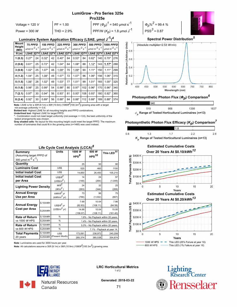
LumiGrow - Pro Series 325ePro325e
Voltage = 120 V. PF = 1.00. PPF (Φp)1 = 540 µmol s-1 Φp%2 = 99.4 %
Power = 300 W. THD = 2.9%. PPF/W (Kp) = 1.8 µmol J-1. PSS3 = 0.87
Luminaire System Application Efficacy (LSAE, µmol J-1)4MountHeight(MH)
75 PPFDµmol m-2 s-1
150 PPFDµmol m-2 s-1
225 PPFDµmol m-2 s-1
300 PPFDµmol m-2 s-1
500 PPFDµmol m-2 s-1
1000 PPFDµmol m-2 s-1
ft (m) LSAE QTY LSAE QTY LSAE QTY LSAE QTY LSAE QTY LSAE QTY1 (0.3) 0.27* 24 0.32* 42 0.40* 64 0.53* 84 0.62* 140 0.70* 276
2 (0.6) 0.61* 25 0.72* 42 1.04* 64 1.08* 88 1.12* 143 1.17* 288
3 (0.9) 1.02* 25 1.07* 48 1.09* 70 1.09* 90 1.11* 150 1.11* 299
4 (1.2) 1.04* 25 1.08* 49 1.07* 72 1.07* 96 1.06* 156 1.06* 315
5 (1.5) 1.06* 28 1.02* 49 1.03* 77 1.01* 99 1.01* 165 1.00* 325
6 (1.8) 0.98* 25 0.99* 54 0.98* 80 0.97* 102 0.96* 170 0.96* 340
7 (2.1) 0.97* 30 0.94* 56 0.93* 81 0.93* 108 0.93* 180 0.92* 360
8 (2.4) 0.92* 30 0.89* 56 0.88* 84 0.88* 112 0.88* 189 0.88* 374
Note- LSAE is for a 30ft (9.1m) x 36ft (10.9m) (1080ft2[100.3m2]) growing area with a target min:average uniformity >= 0.6.Bolded text- Highest LSAE for all mounting heights and PPFD combinations.Underlined text- Highest LSAE for target PPFD.* - Combination could not meet target uniformity (min:average >= 0.6), the best uniformity of the tested arrangements was chosen.Gray shaded cells- No layout for this mounting height could meet the target PPFD. The maximum number of luminaires that could fit in the growing area (n=1485) was used instead.
Spectral Power Distribution5
Photosynthetic Photon Flux (Φp) Comparison6
Photosynthetic Photon Flux Efficacy (Kp) Comparison7
Life Cycle Cost Analysis (LCCA)8Summary(Assuming target PPFD of300 µmol m-2 s-1)
Units 1000 W
HPS9600 W
HPS10This LED11
Quantity 25. 50. 90.
Luminaire Cost US$ 525. 460. 1100.
Initial Install Cost US$ 14,850. 26,450. 105,210.
Initial Install Costper Area
US$/ft2
(US$/m2 )
14.
(148).24.
(264).97.
(1,049).
Lighting Power Density W/ft2
(W/m2 )24.
(263).32.
(344).25.
(269).
Annual EnergyUse per Area
kWh/ft2 yr(kWh/m2 yr)
73.
(790).96.
(1,032).75.
(807).
$.10/kWh 7.69.
(82.83).10.04.
(108.11).7.86.
(84.58).Annual EnergyCost per Area
$.20/kWh
US$/ft2 yr(US$/m2 yr) 14.68.
(158.07).10.04.
(108.11).15.00.
(161.40).
$.10/kWh % 1.6% - No Payback within 20 years..Rate of Returnvs 1000 W HPS $.20/kWh % 1.4% - No Payback within 20 years..
$.10/kWh % 5.0% - No Payback within 20 years..Rate of Returnvs 600 W HPS $.20/kWh % 7.1% - Payback at year 14..
$.10/kWh 173,081. 238,972. 240,208.Total Payments20 years $.20/kWh
US$(Present Worth) 285,374. 385,538. 354,874.
.Note: Luminaires are used for 3000 hours per year.Note: All calculations assume a 30ft (9.1m) x 36ft (10.9m) (1080ft2[100.3m2]) growing area.
Estimated Cumulative CostsOver 20 Years At $0.10/kWh12
Estimated Cumulative CostsOver 20 Years At $0.20/kWh13
LRC Horticultural Metrics1 of 2
Generated: 2018-03-22
71

Iso-PPFD Contours (MH = 3ft (0.9m))14 Photosynthetic Photon Intensity Distribution (Ip, µmol sr-1 s-1) 15
Percentage of Radiant Flux at Different Vertical Angles16
Angle FromNadir
UV% Blue% Red% Far-Red% Blue:RedRatio
Red:Far-Red Ratio
0° 0.05% 23.07% 71.49% 0.52% 0.32 136.55
15° 0.05% 24.32% 70.04% 0.53% 0.35 131.33
30° 0.05% 25.24% 68.93% 0.54% 0.37 126.95
45° 0.06% 30.22% 62.88% 0.57% 0.48 110.11
60° 0.06% 29.37% 63.84% 0.60% 0.46 106.55
75° 0.06% 31.47% 60.85% 0.74% 0.52 81.80
Relative SPD At Different Vertical Angles17
Notes1. Photosynthetic photon flux (PPF) is the rate flow of photons within the photosynthetically active radiation (PAR) range, from 400 nm to 700 nm (ANSI/ASABE S640 JUL2017). It is calculated by multiplying the luminaire SPD by the unweighted PPF action spectrum and summing the total. It represents CO2 assimilation per mole of incident photons, and is analogous to luminaire lumens.2. PPF%: The percentage of the total measured SPD in the PAR range (400 - 700 nm).3. Phytochrome photostationary state (PSS) is a measure of the SPD's impact on phytochrome, a photo-activated plant protein which regulates photomorphogenic responses, seed germination, flowering, and photosynthesis (Sager 1988). A higher value indicates that the SPD will stimulate more of the red form of phytochrome (Pr) than the far-red form (Pfr). PSS is calculated by dividing the integrated SPD multiplied by the Pr function at each wavelength by the integrated SPD multiplied by the sum of the Pr + Pfr function at each wavelength.4. The luminaire system application efficacy (LSAE) metric is the system efficacy for a luminaire layout, at a given mounting height, that meets the PPFD requirements. It is calculated by computing the photosynthetic photon flux density (PPFD, µmol m-2 s-1) at 0.12 m increments for a range of luminaire mounting heights (MH) in a 30ft (9.1m) x 36ft (10.9m) area. Luminaires are arranged in a rectangular array within the growing area, with the luminaire quantity based on the target PPFD level. PPFD values that are >= an assumed minimum-to-average uniformity ratio (> 0.6:1) are used to compute the LSAE.5. The spectral power distribution (SPD) shows the absolute radiant power at each wavelength from 380 nm to 830 nm.6. The luminaire photosynthetic photon flux comparison (Φp) shows this luminaire's PPF value compared to other PPF values for tested horticultural luminaires.7. The luminaire photosynthetic photon flux efficacy comparison (Kp) shows this luminaire's PPF efficacy compared to other PPF efficacies for tested horticultural luminaires.
8. The Life Cycle Cost Analysis (LCCA) table shows the estimated life cycle costs of three luminaire systems meeting the same target PPFD (300 µmol m-2 s-1) over a 20 year life cycle. A 1000 W HPS system and 600 W HPS system are provided as base cases.Assumptions about HID lamp and reflector replacement costs and cleaning costs for all systems are detailed in the LRC report. For LED systems, a sensitivity analysis with 1% failure rates or 25% failure rates at year 10 is included.9. A 1000 W HPS luminaire from P.L. Light Systems, at a 6 ft (1829mm) mounting height, was used for the cost analysis (Med NXT LP 1000W Beta).10. A 600 W HPS luminaire from P.L. Light Systems (tested in 2013), at a 6 ft (1829mm) mounting height, was used for the cost analysis (PL2000 HPS 600W 240V with SON-T PIA lamp).11. The number of luminaires used for each luminaire type in the LCCA analysis is based on the layout that results in the highest LSAE for a target PPFD of 300 µmol m-2 s-1.12. Estimated Cumulative Costs over 20 years at $0.10/kWh. This figure shows the total payments over 20 years for each system type when an hourly energy cost of $0.10/kWh is used. Payback occurs in the year where the system under consideration crosses the 1000 W or 600 W HPS system costs.13. Estimated Cumulative Costs over 20 years at $0.20/kWh. This figure shows the total payments over 20 years for each system type when an hourly energy cost of $0.20/kWh is used.14. The ISO-PPFD contours show the PPFD isolines at fixed intervals from a single luminaire. The luminaire mounting height is based on the layout with the maximum LSAE value with a target PPFD of 300 µmol m-2 s-1 (see LSAE table on page 1). The PPFD is calculated at 0.12 m increments on the workplane. PPFD is analogous to lux.15. The photosynthetic photon intensity distribution (Ip) shows the spatial distribution using two dimensional planes (in units of µmol sr-1 s-1). The red line shows a horizontal slice through the vertical angles where the maximum intensity value occurs. The blue line represents the vertical slice through the luminaire's center at the horizontal angle with the maximum intensity angle. Each of the four rings in the polar diagram represents a 25% change in luminous intensity, with the maximum intensity value represented by the outer ring. Each radiating line represents a 10 degree angular increment.16. The luminaire's SPD was measured at multiple vertical angles (0°, 15°, 30°, 45°, 60° and 75° from nadir) in one horizontal plane. This table shows the percentage of radiant flux at different vertical angles, divided into UV (350 - 400 nm), Blue (400 - 500 nm), Red (600 - 700 nm), and Far-Red (700 - 800 nm). The Blue/Red and Red/Far-Red ratios are also shown.17. This figure shows the relative SPDs, from 380 nm to 830 nm, measured at different vertical angles in one horizontal plane (90 degrees).
LRC Horticultural Metrics2 of 2
Generated: 2018-03-22
72

OSRAM - HL300 Grow LightZELION HL300
Voltage = 120 V. PF = 1.00. PPF (Φp)1 = 788 µmol s-1 Φp%2 = 99.7 %
Power = 374 W. THD = 5.1%. PPF/W (Kp) = 2.1 µmol J-1. PSS3 = 0.88
Luminaire System Application Efficacy (LSAE, µmol J-1)4MountHeight(MH)
75 PPFDµmol m-2 s-1
150 PPFDµmol m-2 s-1
225 PPFDµmol m-2 s-1
300 PPFDµmol m-2 s-1
500 PPFDµmol m-2 s-1
1000 PPFDµmol m-2 s-1
ft (m) LSAE QTY LSAE QTY LSAE QTY LSAE QTY LSAE QTY LSAE QTY1 (0.3) 0.43* 18 0.58* 32 0.64* 45 0.67* 60 1.13* 96 1.49* 187
2 (0.6) 0.73* 18 1.23* 30 1.38* 48 1.34* 63 1.37* 102 1.34* 198
3 (0.9) 1.17* 16 1.29* 32 1.27* 50 1.26* 65 1.24* 105 1.24* 210
4 (1.2) 1.29* 18 1.26* 33 1.23* 48 1.25* 66 1.26* 114 1.13* 222
5 (1.5) 1.21* 21 1.17* 36 1.14* 51 1.15* 69 1.17* 120 1.09* 234
6 (1.8) 1.18* 20 1.16* 36 1.17* 56 1.18* 78 1.02* 128 1.03* 252
7 (2.1) 1.11* 20 1.12* 42 1.11* 62 1.11* 82 0.95* 132 0.96* 264
8 (2.4) 1.03* 22 1.03* 46 1.02* 64 1.02* 84 0.91* 140 0.91* 279
Note- LSAE is for a 30ft (9.1m) x 36ft (10.9m) (1080ft2[100.3m2]) growing area with a target min:average uniformity >= 0.6.Bolded text- Highest LSAE for all mounting heights and PPFD combinations.Underlined text- Highest LSAE for target PPFD.* - Combination could not meet target uniformity (min:average >= 0.6), the best uniformity of the tested arrangements was chosen.Gray shaded cells- No layout for this mounting height could meet the target PPFD. The maximum number of luminaires that could fit in the growing area (n=768) was used instead.
Spectral Power Distribution5
Photosynthetic Photon Flux (Φp) Comparison6
Photosynthetic Photon Flux Efficacy (Kp) Comparison7
Life Cycle Cost Analysis (LCCA)8Summary(Assuming target PPFD of300 µmol m-2 s-1)
Units 1000 W
HPS9600 W
HPS10This LED11
Quantity 25. 50. 63.
Luminaire Cost US$ 525. 460. 1800.
Initial Install Cost US$ 14,850. 26,450. 117,747.
Initial Install Costper Area
US$/ft2
(US$/m2 )
14.
(148).24.
(264).109.
(1,174).
Lighting Power Density W/ft2
(W/m2 )24.
(263).32.
(344).22.
(235).
Annual EnergyUse per Area
kWh/ft2 yr(kWh/m2 yr)
73.
(790).96.
(1,032).65.
(704).
$.10/kWh 7.69.
(82.83).10.04.
(108.11).6.86.
(73.81).Annual EnergyCost per Area
$.20/kWh
US$/ft2 yr(US$/m2 yr) 14.68.
(158.07).10.04.
(108.11).13.09.
(140.86).
$.10/kWh % 2.4% - No Payback within 20 years..Rate of Returnvs 1000 W HPS $.20/kWh % 3.1% - No Payback within 20 years..
$.10/kWh % 5.5% - Payback at year 20..Rate of Returnvs 600 W HPS $.20/kWh % 8.2% - Payback at year 12..
$.10/kWh 173,081. 238,972. 234,376.Total Payments20 years $.20/kWh
US$(Present Worth) 285,374. 385,538. 334,448.
.Note: Luminaires are used for 3000 hours per year.Note: All calculations assume a 30ft (9.1m) x 36ft (10.9m) (1080ft2[100.3m2]) growing area.
Estimated Cumulative CostsOver 20 Years At $0.10/kWh12
Estimated Cumulative CostsOver 20 Years At $0.20/kWh13
LRC Horticultural Metrics1 of 2
Generated: 2018-03-22
73

Iso-PPFD Contours (MH = 2ft (0.6m))14 Photosynthetic Photon Intensity Distribution (Ip, µmol sr-1 s-1) 15
Percentage of Radiant Flux at Different Vertical Angles16
Angle FromNadir
UV% Blue% Red% Far-Red% Blue:RedRatio
Red:Far-Red Ratio
0° 0.04% 15.74% 81.19% 0.32% 0.19 256.32
15° 0.04% 16.44% 80.34% 0.33% 0.20 240.57
30° 0.04% 16.25% 80.41% 0.33% 0.20 242.79
45° 0.04% 15.71% 80.88% 0.36% 0.19 225.47
60° 0.03% 11.70% 86.53% 0.31% 0.14 282.26
75° 0.04% 17.38% 78.32% 0.90% 0.22 87.35
Relative SPD At Different Vertical Angles17
Notes1. Photosynthetic photon flux (PPF) is the rate flow of photons within the photosynthetically active radiation (PAR) range, from 400 nm to 700 nm (ANSI/ASABE S640 JUL2017). It is calculated by multiplying the luminaire SPD by the unweighted PPF action spectrum and summing the total. It represents CO2 assimilation per mole of incident photons, and is analogous to luminaire lumens.2. PPF%: The percentage of the total measured SPD in the PAR range (400 - 700 nm).3. Phytochrome photostationary state (PSS) is a measure of the SPD's impact on phytochrome, a photo-activated plant protein which regulates photomorphogenic responses, seed germination, flowering, and photosynthesis (Sager 1988). A higher value indicates that the SPD will stimulate more of the red form of phytochrome (Pr) than the far-red form (Pfr). PSS is calculated by dividing the integrated SPD multiplied by the Pr function at each wavelength by the integrated SPD multiplied by the sum of the Pr + Pfr function at each wavelength.4. The luminaire system application efficacy (LSAE) metric is the system efficacy for a luminaire layout, at a given mounting height, that meets the PPFD requirements. It is calculated by computing the photosynthetic photon flux density (PPFD, µmol m-2 s-1) at 0.12 m increments for a range of luminaire mounting heights (MH) in a 30ft (9.1m) x 36ft (10.9m) area. Luminaires are arranged in a rectangular array within the growing area, with the luminaire quantity based on the target PPFD level. PPFD values that are >= an assumed minimum-to-average uniformity ratio (> 0.6:1) are used to compute the LSAE.5. The spectral power distribution (SPD) shows the absolute radiant power at each wavelength from 380 nm to 830 nm.6. The luminaire photosynthetic photon flux comparison (Φp) shows this luminaire's PPF value compared to other PPF values for tested horticultural luminaires.7. The luminaire photosynthetic photon flux efficacy comparison (Kp) shows this luminaire's PPF efficacy compared to other PPF efficacies for tested horticultural luminaires.
8. The Life Cycle Cost Analysis (LCCA) table shows the estimated life cycle costs of three luminaire systems meeting the same target PPFD (300 µmol m-2 s-1) over a 20 year life cycle. A 1000 W HPS system and 600 W HPS system are provided as base cases.Assumptions about HID lamp and reflector replacement costs and cleaning costs for all systems are detailed in the LRC report. For LED systems, a sensitivity analysis with 1% failure rates or 25% failure rates at year 10 is included.9. A 1000 W HPS luminaire from P.L. Light Systems, at a 6 ft (1829mm) mounting height, was used for the cost analysis (Med NXT LP 1000W Beta).10. A 600 W HPS luminaire from P.L. Light Systems (tested in 2013), at a 6 ft (1829mm) mounting height, was used for the cost analysis (PL2000 HPS 600W 240V with SON-T PIA lamp).11. The number of luminaires used for each luminaire type in the LCCA analysis is based on the layout that results in the highest LSAE for a target PPFD of 300 µmol m-2 s-1.12. Estimated Cumulative Costs over 20 years at $0.10/kWh. This figure shows the total payments over 20 years for each system type when an hourly energy cost of $0.10/kWh is used. Payback occurs in the year where the system under consideration crosses the 1000 W or 600 W HPS system costs.13. Estimated Cumulative Costs over 20 years at $0.20/kWh. This figure shows the total payments over 20 years for each system type when an hourly energy cost of $0.20/kWh is used.14. The ISO-PPFD contours show the PPFD isolines at fixed intervals from a single luminaire. The luminaire mounting height is based on the layout with the maximum LSAE value with a target PPFD of 300 µmol m-2 s-1 (see LSAE table on page 1). The PPFD is calculated at 0.12 m increments on the workplane. PPFD is analogous to lux.15. The photosynthetic photon intensity distribution (Ip) shows the spatial distribution using two dimensional planes (in units of µmol sr-1 s-1). The red line shows a horizontal slice through the vertical angles where the maximum intensity value occurs. The blue line represents the vertical slice through the luminaire's center at the horizontal angle with the maximum intensity angle. Each of the four rings in the polar diagram represents a 25% change in luminous intensity, with the maximum intensity value represented by the outer ring. Each radiating line represents a 10 degree angular increment.16. The luminaire's SPD was measured at multiple vertical angles (0°, 15°, 30°, 45°, 60° and 75° from nadir) in one horizontal plane. This table shows the percentage of radiant flux at different vertical angles, divided into UV (350 - 400 nm), Blue (400 - 500 nm), Red (600 - 700 nm), and Far-Red (700 - 800 nm). The Blue/Red and Red/Far-Red ratios are also shown.17. This figure shows the relative SPDs, from 380 nm to 830 nm, measured at different vertical angles in one horizontal plane (90 degrees).
LRC Horticultural Metrics2 of 2
Generated: 2018-03-22
74

Philips Lighting - IBRS 10461, 5600 VB, NLGreenPower LED toplighting Deep Red-White-Far Red-Medium Blue
Voltage = 240 V. PF = 1.00. PPF (Φp)1 = 504 µmol s-1 Φp%2 = 99.5 %
Power = 195 W. THD = 7.2%. PPF/W (Kp) = 2.6 µmol J-1. PSS3 = 0.88
Luminaire System Application Efficacy (LSAE, µmol J-1)4MountHeight(MH)
75 PPFDµmol m-2 s-1
150 PPFDµmol m-2 s-1
225 PPFDµmol m-2 s-1
300 PPFDµmol m-2 s-1
500 PPFDµmol m-2 s-1
1000 PPFDµmol m-2 s-1
ft (m) LSAE QTY LSAE QTY LSAE QTY LSAE QTY LSAE QTY LSAE QTY1 (0.3) 0.63* 24 0.79* 44 0.95* 66 1.08* 90 0.84* 144 0.42* 144
2 (0.6) 0.96* 24 1.56* 48 1.36* 72 1.52* 90 1.51* 144 0.13* 144
3 (0.9) 1.07* 24 1.56* 48 1.48* 72 1.56* 96 1.41* 144 0.00* 144
4 (1.2) 1.39* 24 1.49* 50 1.55* 78 1.49* 100 1.33* 144 0.00* 144
5 (1.5) 1.50* 30 1.47* 54 1.46* 78 1.42* 102 1.23* 144 0.00* 144
6 (1.8) 1.43* 30 1.38* 54 1.40* 84 1.37* 108 1.11* 144 0.00* 144
7 (2.1) 1.36* 30 1.32* 56 1.31* 84 1.32* 114 0.93* 144 0.00* 144
8 (2.4) 1.27* 30 1.26* 58 1.26* 90 1.27* 120 0.84* 144 0.00* 144
Note- LSAE is for a 30ft (9.1m) x 36ft (10.9m) (1080ft2[100.3m2]) growing area with a target min:average uniformity >= 0.6.Bolded text- Highest LSAE for all mounting heights and PPFD combinations.Underlined text- Highest LSAE for target PPFD.* - Combination could not meet target uniformity (min:average >= 0.6), the best uniformity of the tested arrangements was chosen.Gray shaded cells- No layout for this mounting height could meet the target PPFD. The maximum number of luminaires that could fit in the growing area (n=144) was used instead.
Spectral Power Distribution5
Photosynthetic Photon Flux (Φp) Comparison6
Photosynthetic Photon Flux Efficacy (Kp) Comparison7
Life Cycle Cost Analysis (LCCA)8Summary(Assuming target PPFD of300 µmol m-2 s-1)
Units 1000 W
HPS9600 W
HPS10This LED11
Quantity 25. 50. 96.
Luminaire Cost US$ 525. 460. 955.
Initial Install Cost US$ 14,850. 26,450. 98,304.
Initial Install Costper Area
US$/ft2
(US$/m2 )
14.
(148).24.
(264).91.
(980).
Lighting Power Density W/ft2
(W/m2 )24.
(263).32.
(344).17.
(187).
Annual EnergyUse per Area
kWh/ft2 yr(kWh/m2 yr)
73.
(790).96.
(1,032).52.
(560).
$.10/kWh 7.69.
(82.83).10.04.
(108.11).5.45.
(58.66).Annual EnergyCost per Area
$.20/kWh
US$/ft2 yr(US$/m2 yr) 14.68.
(158.07).10.04.
(108.11).10.40.
(111.94).
$.10/kWh % 4.3% - No Payback within 20 years..Rate of Returnvs 1000 W HPS $.20/kWh % 6.5% - Payback at year 18..
$.10/kWh % 8.0% - Payback at year 12..Rate of Returnvs 600 W HPS $.20/kWh % 12.6% - Payback at year 7..
$.10/kWh 173,081. 238,972. 195,102.Total Payments20 years $.20/kWh
US$(Present Worth) 285,374. 385,538. 274,630.
.Note: Luminaires are used for 3000 hours per year.Note: All calculations assume a 30ft (9.1m) x 36ft (10.9m) (1080ft2[100.3m2]) growing area.
Estimated Cumulative CostsOver 20 Years At $0.10/kWh12
Estimated Cumulative CostsOver 20 Years At $0.20/kWh13
LRC Horticultural Metrics1 of 2
Generated: 2018-03-22
75

Iso-PPFD Contours (MH = 3ft (0.9m))14 Photosynthetic Photon Intensity Distribution (Ip, µmol sr-1 s-1) 15
Percentage of Radiant Flux at Different Vertical Angles16
Angle FromNadir
UV% Blue% Red% Far-Red% Blue:RedRatio
Red:Far-Red Ratio
0° 0.03% 11.50% 80.87% 0.54% 0.14 150.17
15° 0.03% 10.87% 81.75% 0.54% 0.13 152.66
30° 0.03% 9.25% 84.01% 0.51% 0.11 164.27
45° 0.02% 7.65% 86.10% 0.50% 0.09 171.93
60° 0.03% 9.74% 81.75% 0.59% 0.12 138.12
75° 0.02% 9.39% 82.42% 0.70% 0.11 117.31
Relative SPD At Different Vertical Angles17
Notes1. Photosynthetic photon flux (PPF) is the rate flow of photons within the photosynthetically active radiation (PAR) range, from 400 nm to 700 nm (ANSI/ASABE S640 JUL2017). It is calculated by multiplying the luminaire SPD by the unweighted PPF action spectrum and summing the total. It represents CO2 assimilation per mole of incident photons, and is analogous to luminaire lumens.2. PPF%: The percentage of the total measured SPD in the PAR range (400 - 700 nm).3. Phytochrome photostationary state (PSS) is a measure of the SPD's impact on phytochrome, a photo-activated plant protein which regulates photomorphogenic responses, seed germination, flowering, and photosynthesis (Sager 1988). A higher value indicates that the SPD will stimulate more of the red form of phytochrome (Pr) than the far-red form (Pfr). PSS is calculated by dividing the integrated SPD multiplied by the Pr function at each wavelength by the integrated SPD multiplied by the sum of the Pr + Pfr function at each wavelength.4. The luminaire system application efficacy (LSAE) metric is the system efficacy for a luminaire layout, at a given mounting height, that meets the PPFD requirements. It is calculated by computing the photosynthetic photon flux density (PPFD, µmol m-2 s-1) at 0.12 m increments for a range of luminaire mounting heights (MH) in a 30ft (9.1m) x 36ft (10.9m) area. Luminaires are arranged in a rectangular array within the growing area, with the luminaire quantity based on the target PPFD level. PPFD values that are >= an assumed minimum-to-average uniformity ratio (> 0.6:1) are used to compute the LSAE.5. The spectral power distribution (SPD) shows the absolute radiant power at each wavelength from 380 nm to 830 nm.6. The luminaire photosynthetic photon flux comparison (Φp) shows this luminaire's PPF value compared to other PPF values for tested horticultural luminaires.7. The luminaire photosynthetic photon flux efficacy comparison (Kp) shows this luminaire's PPF efficacy compared to other PPF efficacies for tested horticultural luminaires.
8. The Life Cycle Cost Analysis (LCCA) table shows the estimated life cycle costs of three luminaire systems meeting the same target PPFD (300 µmol m-2 s-1) over a 20 year life cycle. A 1000 W HPS system and 600 W HPS system are provided as base cases.Assumptions about HID lamp and reflector replacement costs and cleaning costs for all systems are detailed in the LRC report. For LED systems, a sensitivity analysis with 1% failure rates or 25% failure rates at year 10 is included.9. A 1000 W HPS luminaire from P.L. Light Systems, at a 6 ft (1829mm) mounting height, was used for the cost analysis (Med NXT LP 1000W Beta).10. A 600 W HPS luminaire from P.L. Light Systems (tested in 2013), at a 6 ft (1829mm) mounting height, was used for the cost analysis (PL2000 HPS 600W 240V with SON-T PIA lamp).11. The number of luminaires used for each luminaire type in the LCCA analysis is based on the layout that results in the highest LSAE for a target PPFD of 300 µmol m-2 s-1.12. Estimated Cumulative Costs over 20 years at $0.10/kWh. This figure shows the total payments over 20 years for each system type when an hourly energy cost of $0.10/kWh is used. Payback occurs in the year where the system under consideration crosses the 1000 W or 600 W HPS system costs.13. Estimated Cumulative Costs over 20 years at $0.20/kWh. This figure shows the total payments over 20 years for each system type when an hourly energy cost of $0.20/kWh is used.14. The ISO-PPFD contours show the PPFD isolines at fixed intervals from a single luminaire. The luminaire mounting height is based on the layout with the maximum LSAE value with a target PPFD of 300 µmol m-2 s-1 (see LSAE table on page 1). The PPFD is calculated at 0.12 m increments on the workplane. PPFD is analogous to lux.15. The photosynthetic photon intensity distribution (Ip) shows the spatial distribution using two dimensional planes (in units of µmol sr-1 s-1). The red line shows a horizontal slice through the vertical angles where the maximum intensity value occurs. The blue line represents the vertical slice through the luminaire's center at the horizontal angle with the maximum intensity angle. Each of the four rings in the polar diagram represents a 25% change in luminous intensity, with the maximum intensity value represented by the outer ring. Each radiating line represents a 10 degree angular increment.16. The luminaire's SPD was measured at multiple vertical angles (0°, 15°, 30°, 45°, 60° and 75° from nadir) in one horizontal plane. This table shows the percentage of radiant flux at different vertical angles, divided into UV (350 - 400 nm), Blue (400 - 500 nm), Red (600 - 700 nm), and Far-Red (700 - 800 nm). The Blue/Red and Red/Far-Red ratios are also shown.17. This figure shows the relative SPDs, from 380 nm to 830 nm, measured at different vertical angles in one horizontal plane (90 degrees).
LRC Horticultural Metrics2 of 2
Generated: 2018-03-22
76

P.L. Light Systems - HortiLED TopHortiLED TOP-150 degree distribution angle-120-277V-Full Spectrum-0-10 V dimming
Voltage = 240 V. PF = 0.95. PPF (Φp)1 = 696 µmol s-1 Φp%2 = 98.8 %
Power = 330 W. THD = 13.5%. PPF/W (Kp) = 2.1 µmol J-1. PSS3 = 0.86
Luminaire System Application Efficacy (LSAE, µmol J-1)4MountHeight(MH)
75 PPFDµmol m-2 s-1
150 PPFDµmol m-2 s-1
225 PPFDµmol m-2 s-1
300 PPFDµmol m-2 s-1
500 PPFDµmol m-2 s-1
1000 PPFDµmol m-2 s-1
ft (m) LSAE QTY LSAE QTY LSAE QTY LSAE QTY LSAE QTY LSAE QTY1 (0.3) 0.45* 18 0.62* 36 0.71* 48 0.77* 66 0.92* 108 0.76* 198
2 (0.6) 0.86* 21 1.22* 36 1.26* 54 1.23* 68 1.25* 114 1.20* 198
3 (0.9) 1.17* 21 1.17* 36 1.23* 54 1.17* 72 1.22* 120 1.09* 198
4 (1.2) 1.14* 21 1.21* 42 1.19* 60 1.13* 76 1.16* 126 0.96* 198
5 (1.5) 1.16* 24 1.12* 42 1.10* 60 1.12* 84 1.10* 136 0.78* 198
6 (1.8) 1.10* 24 1.04* 42 1.05* 66 1.06* 90 1.04* 142 0.66* 198
7 (2.1) 1.02* 24 1.00* 48 0.99* 68 0.99* 90 1.00* 156 0.53* 198
8 (2.4) 0.95* 24 0.93* 48 0.94* 72 0.94* 96 0.94* 162 0.41* 198
Note- LSAE is for a 30ft (9.1m) x 36ft (10.9m) (1080ft2[100.3m2]) growing area with a target min:average uniformity >= 0.6.Bolded text- Highest LSAE for all mounting heights and PPFD combinations.Underlined text- Highest LSAE for target PPFD.* - Combination could not meet target uniformity (min:average >= 0.6), the best uniformity of the tested arrangements was chosen.Gray shaded cells- No layout for this mounting height could meet the target PPFD. The maximum number of luminaires that could fit in the growing area (n=198) was used instead.
Spectral Power Distribution5
Photosynthetic Photon Flux (Φp) Comparison6
Photosynthetic Photon Flux Efficacy (Kp) Comparison7
Life Cycle Cost Analysis (LCCA)8Summary(Assuming target PPFD of300 µmol m-2 s-1)
Units 1000 W
HPS9600 W
HPS10This LED11
Quantity 25. 50. 68.
Luminaire Cost US$ 525. 460. 1186.
Initial Install Cost US$ 14,850. 26,450. 85,340.
Initial Install Costper Area
US$/ft2
(US$/m2 )
14.
(148).24.
(264).79.
(851).
Lighting Power Density W/ft2
(W/m2 )24.
(263).32.
(344).21.
(224).
Annual EnergyUse per Area
kWh/ft2 yr(kWh/m2 yr)
73.
(790).96.
(1,032).62.
(672).
$.10/kWh 7.69.
(82.83).10.04.
(108.11).6.54.
(70.40).Annual EnergyCost per Area
$.20/kWh
US$/ft2 yr(US$/m2 yr) 14.68.
(158.07).10.04.
(108.11).12.48.
(134.35).
$.10/kWh % 3.7% - No Payback within 20 years..Rate of Returnvs 1000 W HPS $.20/kWh % 5.1% - No Payback within 20 years..
$.10/kWh % 8.0% - Payback at year 11..Rate of Returnvs 600 W HPS $.20/kWh % 12.1% - Payback at year 7..
$.10/kWh 173,081. 238,972. 197,081.Total Payments20 years $.20/kWh
US$(Present Worth) 285,374. 385,538. 292,529.
.Note: Luminaires are used for 3000 hours per year.Note: All calculations assume a 30ft (9.1m) x 36ft (10.9m) (1080ft2[100.3m2]) growing area.
Estimated Cumulative CostsOver 20 Years At $0.10/kWh12
Estimated Cumulative CostsOver 20 Years At $0.20/kWh13
LRC Horticultural Metrics1 of 2
Generated: 2018-03-22
77

Iso-PPFD Contours (MH = 2ft (0.6m))14 Photosynthetic Photon Intensity Distribution (Ip, µmol sr-1 s-1) 15
Percentage of Radiant Flux at Different Vertical Angles16
Angle FromNadir
UV% Blue% Red% Far-Red% Blue:RedRatio
Red:Far-Red Ratio
0° 0.09% 31.90% 37.13% 1.09% 0.86 34.13
15° 0.09% 31.40% 37.59% 1.08% 0.84 34.77
30° 0.08% 29.80% 39.31% 1.05% 0.76 37.48
45° 0.08% 27.45% 41.01% 1.03% 0.67 39.97
60° 0.07% 24.99% 42.60% 1.01% 0.59 42.34
75° 0.08% 27.97% 32.88% 1.17% 0.85 28.22
Relative SPD At Different Vertical Angles17
Notes1. Photosynthetic photon flux (PPF) is the rate flow of photons within the photosynthetically active radiation (PAR) range, from 400 nm to 700 nm (ANSI/ASABE S640 JUL2017). It is calculated by multiplying the luminaire SPD by the unweighted PPF action spectrum and summing the total. It represents CO2 assimilation per mole of incident photons, and is analogous to luminaire lumens.2. PPF%: The percentage of the total measured SPD in the PAR range (400 - 700 nm).3. Phytochrome photostationary state (PSS) is a measure of the SPD's impact on phytochrome, a photo-activated plant protein which regulates photomorphogenic responses, seed germination, flowering, and photosynthesis (Sager 1988). A higher value indicates that the SPD will stimulate more of the red form of phytochrome (Pr) than the far-red form (Pfr). PSS is calculated by dividing the integrated SPD multiplied by the Pr function at each wavelength by the integrated SPD multiplied by the sum of the Pr + Pfr function at each wavelength.4. The luminaire system application efficacy (LSAE) metric is the system efficacy for a luminaire layout, at a given mounting height, that meets the PPFD requirements. It is calculated by computing the photosynthetic photon flux density (PPFD, µmol m-2 s-1) at 0.12 m increments for a range of luminaire mounting heights (MH) in a 30ft (9.1m) x 36ft (10.9m) area. Luminaires are arranged in a rectangular array within the growing area, with the luminaire quantity based on the target PPFD level. PPFD values that are >= an assumed minimum-to-average uniformity ratio (> 0.6:1) are used to compute the LSAE.5. The spectral power distribution (SPD) shows the absolute radiant power at each wavelength from 380 nm to 830 nm.6. The luminaire photosynthetic photon flux comparison (Φp) shows this luminaire's PPF value compared to other PPF values for tested horticultural luminaires.7. The luminaire photosynthetic photon flux efficacy comparison (Kp) shows this luminaire's PPF efficacy compared to other PPF efficacies for tested horticultural luminaires.
8. The Life Cycle Cost Analysis (LCCA) table shows the estimated life cycle costs of three luminaire systems meeting the same target PPFD (300 µmol m-2 s-1) over a 20 year life cycle. A 1000 W HPS system and 600 W HPS system are provided as base cases.Assumptions about HID lamp and reflector replacement costs and cleaning costs for all systems are detailed in the LRC report. For LED systems, a sensitivity analysis with 1% failure rates or 25% failure rates at year 10 is included.9. A 1000 W HPS luminaire from P.L. Light Systems, at a 6 ft (1829mm) mounting height, was used for the cost analysis (Med NXT LP 1000W Beta).10. A 600 W HPS luminaire from P.L. Light Systems (tested in 2013), at a 6 ft (1829mm) mounting height, was used for the cost analysis (PL2000 HPS 600W 240V with SON-T PIA lamp).11. The number of luminaires used for each luminaire type in the LCCA analysis is based on the layout that results in the highest LSAE for a target PPFD of 300 µmol m-2 s-1.12. Estimated Cumulative Costs over 20 years at $0.10/kWh. This figure shows the total payments over 20 years for each system type when an hourly energy cost of $0.10/kWh is used. Payback occurs in the year where the system under consideration crosses the 1000 W or 600 W HPS system costs.13. Estimated Cumulative Costs over 20 years at $0.20/kWh. This figure shows the total payments over 20 years for each system type when an hourly energy cost of $0.20/kWh is used.14. The ISO-PPFD contours show the PPFD isolines at fixed intervals from a single luminaire. The luminaire mounting height is based on the layout with the maximum LSAE value with a target PPFD of 300 µmol m-2 s-1 (see LSAE table on page 1). The PPFD is calculated at 0.12 m increments on the workplane. PPFD is analogous to lux.15. The photosynthetic photon intensity distribution (Ip) shows the spatial distribution using two dimensional planes (in units of µmol sr-1 s-1). The red line shows a horizontal slice through the vertical angles where the maximum intensity value occurs. The blue line represents the vertical slice through the luminaire's center at the horizontal angle with the maximum intensity angle. Each of the four rings in the polar diagram represents a 25% change in luminous intensity, with the maximum intensity value represented by the outer ring. Each radiating line represents a 10 degree angular increment.16. The luminaire's SPD was measured at multiple vertical angles (0°, 15°, 30°, 45°, 60° and 75° from nadir) in one horizontal plane. This table shows the percentage of radiant flux at different vertical angles, divided into UV (350 - 400 nm), Blue (400 - 500 nm), Red (600 - 700 nm), and Far-Red (700 - 800 nm). The Blue/Red and Red/Far-Red ratios are also shown.17. This figure shows the relative SPDs, from 380 nm to 830 nm, measured at different vertical angles in one horizontal plane (90 degrees).
LRC Horticultural Metrics2 of 2
Generated: 2018-03-22
78

Sunlight Supply - 906420AgroLED 720 Dio-Watt Full Spectrum Low Pro 120 - 240 Volt 90 Optics
Voltage = 120 V. PF = 0.99. PPF (Φp)1 = 575 µmol s-1 Φp%2 = 96.9 %
Power = 414 W. THD = 7.9%. PPF/W (Kp) = 1.4 µmol J-1. PSS3 = 0.87
Luminaire System Application Efficacy (LSAE, µmol J-1)4MountHeight(MH)
75 PPFDµmol m-2 s-1
150 PPFDµmol m-2 s-1
225 PPFDµmol m-2 s-1
300 PPFDµmol m-2 s-1
500 PPFDµmol m-2 s-1
1000 PPFDµmol m-2 s-1
ft (m) LSAE QTY LSAE QTY LSAE QTY LSAE QTY LSAE QTY LSAE QTY1 (0.3) 0.20* 20 0.23* 40 0.27* 60 0.33* 78 0.40* 135 0.27* 135
2 (0.6) 0.24* 20 0.37* 40 0.50* 60 0.56* 78 0.77* 135 0.17* 135
3 (0.9) 0.34* 20 0.53* 42 0.73* 60 0.87* 78 0.91* 135 0.01* 135
4 (1.2) 0.44* 20 0.66* 42 0.87* 63 0.88* 80 0.87* 135 0.00* 135
5 (1.5) 0.74* 24 0.82* 42 0.86* 63 0.86* 84 0.84* 135 0.00* 135
6 (1.8) 0.84* 24 0.83* 42 0.84* 63 0.84* 84 0.82* 135 0.00* 135
7 (2.1) 0.84* 25 0.82* 42 0.82* 64 0.82* 88 0.79* 135 0.00* 135
8 (2.4) 0.85* 25 0.81* 45 0.80* 66 0.79* 88 0.75* 135 0.00* 135
Note- LSAE is for a 30ft (9.1m) x 36ft (10.9m) (1080ft2[100.3m2]) growing area with a target min:average uniformity >= 0.6.Bolded text- Highest LSAE for all mounting heights and PPFD combinations.Underlined text- Highest LSAE for target PPFD.* - Combination could not meet target uniformity (min:average >= 0.6), the best uniformity of the tested arrangements was chosen.Gray shaded cells- No layout for this mounting height could meet the target PPFD. The maximum number of luminaires that could fit in the growing area (n=135) was used instead.
Spectral Power Distribution5
Photosynthetic Photon Flux (Φp) Comparison6
Photosynthetic Photon Flux Efficacy (Kp) Comparison7
Life Cycle Cost Analysis (LCCA)8Summary(Assuming target PPFD of300 µmol m-2 s-1)
Units 1000 W
HPS9600 W
HPS10This LED11
Quantity 25. 50. 80.
Luminaire Cost US$ 525. 460. 765.
Initial Install Cost US$ 14,850. 26,450. 66,720.
Initial Install Costper Area
US$/ft2
(US$/m2 )
14.
(148).24.
(264).62.
(665).
Lighting Power Density W/ft2
(W/m2 )24.
(263).32.
(344).31.
(330).
Annual EnergyUse per Area
kWh/ft2 yr(kWh/m2 yr)
73.
(790).96.
(1,032).92.
(991).
$.10/kWh 7.69.
(82.83).10.04.
(108.11).9.64.
(103.81).Annual EnergyCost per Area
$.20/kWh
US$/ft2 yr(US$/m2 yr) 14.68.
(158.07).10.04.
(108.11).18.40.
(198.10).
$.10/kWh % <0.0% - No Payback within 20 years..Rate of Returnvs 1000 W HPS $.20/kWh % <0.0% - No Payback within 20 years..
$.10/kWh % 5.2% - Payback at year 17..Rate of Returnvs 600 W HPS $.20/kWh % 5.8% - Payback at year 14..
$.10/kWh 173,081. 238,972. 229,245.Total Payments20 years $.20/kWh
US$(Present Worth) 285,374. 385,538. 369,983.
.Note: Luminaires are used for 3000 hours per year.Note: All calculations assume a 30ft (9.1m) x 36ft (10.9m) (1080ft2[100.3m2]) growing area.
Estimated Cumulative CostsOver 20 Years At $0.10/kWh12
Estimated Cumulative CostsOver 20 Years At $0.20/kWh13
LRC Horticultural Metrics1 of 2
Generated: 2018-03-22
79
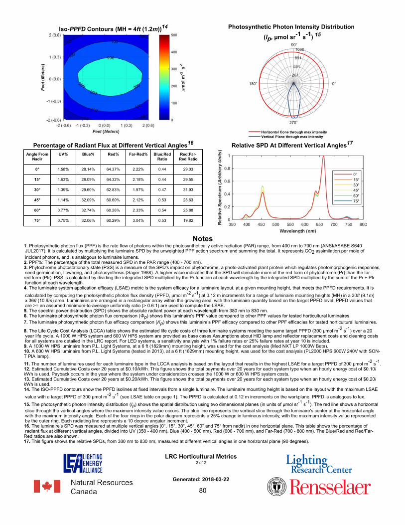
Iso-PPFD Contours (MH = 4ft (1.2m))14 Photosynthetic Photon Intensity Distribution (Ip, µmol sr-1 s-1) 15
Percentage of Radiant Flux at Different Vertical Angles16
Angle FromNadir
UV% Blue% Red% Far-Red% Blue:RedRatio
Red:Far-Red Ratio
0° 1.58% 28.14% 64.37% 2.22% 0.44 29.03
15° 1.63% 28.09% 64.32% 2.18% 0.44 29.55
30° 1.39% 29.60% 62.83% 1.97% 0.47 31.93
45° 1.14% 32.09% 60.60% 2.12% 0.53 28.63
60° 0.77% 32.74% 60.26% 2.33% 0.54 25.88
75° 0.75% 32.06% 60.29% 3.04% 0.53 19.82
Relative SPD At Different Vertical Angles17
Notes1. Photosynthetic photon flux (PPF) is the rate flow of photons within the photosynthetically active radiation (PAR) range, from 400 nm to 700 nm (ANSI/ASABE S640 JUL2017). It is calculated by multiplying the luminaire SPD by the unweighted PPF action spectrum and summing the total. It represents CO2 assimilation per mole of incident photons, and is analogous to luminaire lumens.2. PPF%: The percentage of the total measured SPD in the PAR range (400 - 700 nm).3. Phytochrome photostationary state (PSS) is a measure of the SPD's impact on phytochrome, a photo-activated plant protein which regulates photomorphogenic responses, seed germination, flowering, and photosynthesis (Sager 1988). A higher value indicates that the SPD will stimulate more of the red form of phytochrome (Pr) than the far-red form (Pfr). PSS is calculated by dividing the integrated SPD multiplied by the Pr function at each wavelength by the integrated SPD multiplied by the sum of the Pr + Pfr function at each wavelength.4. The luminaire system application efficacy (LSAE) metric is the system efficacy for a luminaire layout, at a given mounting height, that meets the PPFD requirements. It is calculated by computing the photosynthetic photon flux density (PPFD, µmol m-2 s-1) at 0.12 m increments for a range of luminaire mounting heights (MH) in a 30ft (9.1m) x 36ft (10.9m) area. Luminaires are arranged in a rectangular array within the growing area, with the luminaire quantity based on the target PPFD level. PPFD values that are >= an assumed minimum-to-average uniformity ratio (> 0.6:1) are used to compute the LSAE.5. The spectral power distribution (SPD) shows the absolute radiant power at each wavelength from 380 nm to 830 nm.6. The luminaire photosynthetic photon flux comparison (Φp) shows this luminaire's PPF value compared to other PPF values for tested horticultural luminaires.7. The luminaire photosynthetic photon flux efficacy comparison (Kp) shows this luminaire's PPF efficacy compared to other PPF efficacies for tested horticultural luminaires.
8. The Life Cycle Cost Analysis (LCCA) table shows the estimated life cycle costs of three luminaire systems meeting the same target PPFD (300 µmol m-2 s-1) over a 20 year life cycle. A 1000 W HPS system and 600 W HPS system are provided as base cases.Assumptions about HID lamp and reflector replacement costs and cleaning costs for all systems are detailed in the LRC report. For LED systems, a sensitivity analysis with 1% failure rates or 25% failure rates at year 10 is included.9. A 1000 W HPS luminaire from P.L. Light Systems, at a 6 ft (1829mm) mounting height, was used for the cost analysis (Med NXT LP 1000W Beta).10. A 600 W HPS luminaire from P.L. Light Systems (tested in 2013), at a 6 ft (1829mm) mounting height, was used for the cost analysis (PL2000 HPS 600W 240V with SON-T PIA lamp).11. The number of luminaires used for each luminaire type in the LCCA analysis is based on the layout that results in the highest LSAE for a target PPFD of 300 µmol m-2 s-1.12. Estimated Cumulative Costs over 20 years at $0.10/kWh. This figure shows the total payments over 20 years for each system type when an hourly energy cost of $0.10/kWh is used. Payback occurs in the year where the system under consideration crosses the 1000 W or 600 W HPS system costs.13. Estimated Cumulative Costs over 20 years at $0.20/kWh. This figure shows the total payments over 20 years for each system type when an hourly energy cost of $0.20/kWh is used.14. The ISO-PPFD contours show the PPFD isolines at fixed intervals from a single luminaire. The luminaire mounting height is based on the layout with the maximum LSAE value with a target PPFD of 300 µmol m-2 s-1 (see LSAE table on page 1). The PPFD is calculated at 0.12 m increments on the workplane. PPFD is analogous to lux.15. The photosynthetic photon intensity distribution (Ip) shows the spatial distribution using two dimensional planes (in units of µmol sr-1 s-1). The red line shows a horizontal slice through the vertical angles where the maximum intensity value occurs. The blue line represents the vertical slice through the luminaire's center at the horizontal angle with the maximum intensity angle. Each of the four rings in the polar diagram represents a 25% change in luminous intensity, with the maximum intensity value represented by the outer ring. Each radiating line represents a 10 degree angular increment.16. The luminaire's SPD was measured at multiple vertical angles (0°, 15°, 30°, 45°, 60° and 75° from nadir) in one horizontal plane. This table shows the percentage of radiant flux at different vertical angles, divided into UV (350 - 400 nm), Blue (400 - 500 nm), Red (600 - 700 nm), and Far-Red (700 - 800 nm). The Blue/Red and Red/Far-Red ratios are also shown.17. This figure shows the relative SPDs, from 380 nm to 830 nm, measured at different vertical angles in one horizontal plane (90 degrees).
LRC Horticultural Metrics2 of 2
Generated: 2018-03-22
80