LECTURES ON TIDES

UNIS, Longyearbyen, 26 - 30 Sept. 2011

by

B. Gjevik

Department of Mathematics, University of Oslo

P.O.Box 1053 Blindern, Oslo, Norway

email: bjorng@math.uio.no

1

Contents

1 Introduction 3

2 Tide generating force 5

3 Harmonic decomposition of the tide generating force 10

4 Ocean response 11

5 Harmonic constants and tidal predictions 11

6 Harmonic analysis of tidal records 15

7 Laplace’s tidal equation 17

8 Free wave solution to LTE. Kelvin waves. 18

9 Numerical models 21

10 Tidal charts for the Barents Sea 21

11 Tidal currents 27

12 Drift and dispersion of particles in the tidal flow 28

13 Mean sea level (MSL) 30

14 Exercises 32

2

1 Introduction

The periodic rise and fall of the sea surface has fascinated man from the earliest ages.Obviously people must early have noticed the connection between high and low waterand the position of the Moon and the Sun. Due to the regularity of the phenomena itbecame closely associated with the flow of time as the very name tides indicates.

When Newton (1697) first formulated the theory of gravitation he also discoveredthe nature of the tide generating force. Newton’s equilibrium theory of tides explainedthe observed dominant semidiurnal periodicity of ocean tides. Up to then it had beena mystery that high water occurs both with Moon overhead and also about 12 hourslater when the Moon is on the other side of the earth. Today Newton’s equilibriumtheory (see section 2) provides the correct tide generating force to which the oceansrespond hydrodynamically in a rather complicated fashion. Although Newton discov-ered the true astronomic nature of the tide, it was Laplace (1775) who derived thefirst hydrodynamic equations of ocean tides. Laplace’s tidal equations contain the tidegenerating force in terms of Newton’s equilibrium tide as the forcing function.

Figure 1: The Moon is barren and lifeless, but its gravitational force induces strong tidal currentsin the world’s oceans and thereby affects life on the Earth. Here the Moon is photographed in perigeeposition when it is closest to the Earth.

Due to the complexity of Laplace’s tidal equations little progress was made insolving these equations with realistic bottom topography and coastlines before powerful

3

Periodic cycles of the Moon

There are four important cycles of the Moon with periods 27–29 days.

Nr. Type Period(mean solar day)

1 Recurrence of Moon’s phase (synodic Moon). 29.53062 Oscillation in Moon’s distance.

from Earth (anomalistic Moon). 27.55463 Oscillation in the Moon’s declination. 27.21224 Time of one orbit around the ecliptic relativ

to the vernal equinox (sidereal Moon). 27.3216

If two periodic events (signals), recurring with period T1 and T2 respectively, are in phase at timet = 0 they will be in phase again after t = Tn = nT1 where the integer number n is determinedfrom nT1 = (n + 1)T2. This leads to n = T2/(T1 − T2) and Tn = T1T2/(T1 − T2) ( T1 > T2).With T1= 29,5306 days and T2 = 27,5546 days we find that it will be Tn = 1.13 year betweenthe recurrence of perigee at either full or new Moon. Similarly it will take 8.9 years betweeneach time perigee coincides with the vernal equinox.

computers became available. Since then Laplace’s equations have been the basis of mostmodern tidal modelling.

The observation and mathematical treatments of tides were greatly advanced byLord Kelvin (Thomson, 1868) who introduced the method of harmonic analysis of tides.Both the astronomical forcing and the responding ocean tide are represented as a seriesof harmonic tidal components each with its characteristic frequency, determined fromthe regular almost periodic motion of the Moon and the Sun. With this representationthe time dependent ocean tides, can be accurately described when a few time indepen-dent harmonic constants in terms of amplitude and phases are known. The harmonicconstants are characteristic for every geographical point in the ocean and along thecoasts. These constants may be determined by harmonic analysis of observed timeseries of sea level changes, with regular and sufficient frequent time sampling, or bysolving the Laplace’s tidal equations with realistic bottom topography and coastlineconfigurations.

The tides particularly in coastal waters appear as a markly dominant part of theocean current variability. Since sea level changes and shifting currents associated withthe tides are of great importance for all maritime activity , coastal engineering andmanagement there is an enormous number of scientific publications devoted to thesubject. The reviews by Cartwright (1977), Schwiderski (1980, 1986), and Davies etal. (1996) survey central parts of the literature. It is impossible to cover this vast subjectwithin the frame of this short lecture series. We will therefore restrict to discuss insome detail, three important aspect, the nature of the tide generating force, harmonicanalysis of tide and some aspects of tidal modelling. The presentation and examplesin this lecture series rely heavily on my own and my co-workers research on tides andmay for this reason be somewhat biased with respect to citations and references.

4

2 Tide generating force

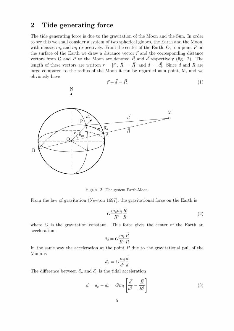
The tide generating force is due to the gravitation of the Moon and the Sun. In orderto see this we shall consider a system of two spherical globes, the Earth and the Moon,with masses me and ml respectively. From the center of the Earth, O, to a point P onthe surface of the Earth we draw a distance vector ~r and the corresponding distancevectors from O and P to the Moon are denoted ~R and ~d respectively (fig. 2). The

length of these vectors are written r = |~r|, R = |~R| and d = |~d|. Since d and R arelarge compared to the radius of the Moon it can be regarded as a point, M, and weobviously have

~r + ~d = ~R (1)

B

OA

N

P

M

~r θm

~d

~R

~ar

~ah

Figure 2: The system Earth-Moon.

From the law of gravitation (Newton 1697), the gravitational force on the Earth is

Gmeml

R2

~R

R(2)

where G is the gravitation constant. This force gives the center of the Earth anacceleration.

~a0 = Gml

R2

~R

R

In the same way the acceleration at the point P due to the gravitational pull of theMoon is

~ap = Gml

d2

~d

d

The difference between ~ap and ~ao is the tidal acceleration

~a = ~ap − ~ao = Gml

[~d

d3−

~R

R3

](3)

5

which corresponds to a tidal force pr unit mass. The vector ~a is obviously containedin the plane through O, P and M .From the trigonometric cosines relation for the triangle OPM

d2 = R2 + r2 − 2Rr cos θm

where angle θm is the angular zenit distance of the Moon. Hence

d = R

√1 − 2

r

Rcos θm +

r2

R2

By expanding the square root in a series after the small parameter rR

and neglecting

terms of order(

rR

)2.

d ∼= R[1 − r

Rcos θm

]+ O

( r

R

)2

Again by series expansion

1

d3=

1

R3(1 − rR

cos θm)3

∼=(1 + 3 r

Rcos θm)

R3

By using the latter relation together with eq. (1), the tidal acceleration, eq. (3), canbe written:

~a =Gmlr

R3

[3

~R

Rcos θm − ~r

r

](4)

When introducing the acceleration of gravity at the Earth’s surface

g =Gme

r2

the expression (4) can be written

~a = gml

me

( r

R

)3

[3

~R

Rcos θm − ~r

r

](5)

which shows that the tidal acceleration is a very small fraction of g. With parametersfor the Earth–Moon system, ml

me= 0.012, r

R= 0.017 the fraction is of the order 10−7.

Equation (5) shows that ~a is a sum of a vertical vector always pointing downward

along the vertical and a vector in the direction ~R i. e. towards the Moon for θm < π2

and opposite ~R when π2

< θm < π. Hence there will be a component of the accelerationdirected either towards the point A under the Moon or towards the antipodal point Bon the other side of the Earth (fig. 3).The vector ~a can be decomposed in a vertical component, ar, and a horizontal com-ponent, ah. The latter being directed along the great circle arch APB (fig.2). Since~R · ~r = Rr cos θm we have

ar = ~a · ~r

r= g

ml

me

( r

R

)3

[3 cos2 θm − 1] (6)

6

BO

Ato Moonθm

Figure 3: The direction of the tidal acceleration.

and since |~R × ~r | = Rr sin θm

ah =∣∣∣~a × ~r

r

∣∣∣ =3

2gml

me

( r

R

)3

sin 2θm (7)

Here we can introduce the Moon’s horizontal parallax πm defined by

sin πm =r

R

which is a commonly used parameter for the position of the Moon.Imaging now that the Earth is covered by a thin sheet of water subject to the tide

generating force of the Moon. In order to be in equilibrium the surface of the waterwill deform in order to set up an adverse pressure gradient counteracting the horizontaltidal force. The equilibrium condition is

−g∂ηm

r∂θm

− 3

2gml

me

sin3 πm sin 2θm = 0

where ηm is the vertical displacement of the water. By integration we obtain

ηm =3

4

ml

me

r sin3 πm cos 2θm + C

where C is a constant of integration which is determined by the requirement that thereis no change in water volume by the deformation. This leads to C = 1

3and

ηm =1

4

ml

me

r sin3 πm(3 cos 2θm + 1) (8)

This expression shows that there will be high water under the Moon at A and also thepoint B on the opposite side of the Earth. A zone of low water extends around theglobe with lowest water level for θm = π

2as sketched in figure 5.

7

Figure 4: The horizontal component of the tidal force is directed toward a point right under theMoon and the image on the opposite side of the Earth. Here the Moon stands over North Africa andthe image is located north of New Zeland in the Pacific Ocean. The same force field will appear if theMoon was located above the image point. As the Earth rotates the field will move westward.

With the Moon moving in the equatorial plane there will, for each location on theEarth, be high water when the Moon passes the meridian and another equally highwater about 12.4 hours later when the Moon is on the opposite side of the Earth.Hence, the expression (8) explains nicely the semi-diurnal variation of sea level. Whenthe Moon has a northern or southern declination there will be an asymmetry betweentwo consecutive high waters. Therefore equation (8) also explains the diurnal equalityi.e. the difference in sea level rise between two consecutive high water. The surfacedisplacement given by eq. (8) is called the equilibrium tide and in absence of continentit is thought to follow the Moon when the earth rotates. It corresponds to the idealizedsituation where the water masses adjust instantaneous to the motion of the Moon.

Table 1 Astronomical constants.

Mass of the Earth: me 5.974·1024 kgMass of the Sun: ms 1.991·1030 kgMass of the Moon: ml 7.347·1022 kgMean distance Earth-Moon R 3.844·10 5 kmMean distance Earth-Sun R 1.496·10 8 kmRadius of the Earth r 6.370·10 3 km

The equilibrium tide is often used as a potential for the tide generating force. Thestrength of the horizontal component of the tidal acceleration (7) and the equilibriumtide (8) will vary with the position of the Moon and its distance from the Earth.Maximum tidal acceleration will occur when the Moon is closest to the Earth (perigee)

8

B O A

to Moon

Figure 5: The equilibrium tide

and minimum acceleration when the Moon is in apogean position. The variation theacceleration from minimum to maximum is about 20% of the mean value.

Here we have only established, to lowest order of accuracy, the expression for theequilibrium tide due to the action of the Moon. A similar expression will clearly alsoappear from the action of the Sun

ηs =1

4

ms

me

r sin3 πs(3 cos 2θs + 1)

where ms and πs denote the mass and the horizontal parallax of the Sun respectively,and θs is zenit distance of the Sun. Although the mass of the Sun is much larger thanthe mass of the Moon the parallax for the Sun is much less than the parallax of theMoon. The equilibrium tide due to the Sun is therefore about half of the Moon’s.The combined effect of the Moon and the Sun leads to an expression for the totalequilibrium tide

η = ηm + ηs (9)

With the astronomical constants in table 1 we find the maximum values of the equi-librium tide ηm =0.35 m and |ηs| =0.15 m. Hence the maximum amplitude of thecombined equilibrium tide from the Moon and the Sun will be 0.50 m. This is consid-erably less then the ocean tide in most places and we will later, in section 4, see howthe equilibrium tide is amplified in the ocean. Since the position of the Moon and theSun can be calculated with a high degree of accuracy the parallax and zenit distancesis known as highly accurate functions of time. Hence we can calculate the spatial andtemporal variation of the equilibrium tide or equivalently the tide generating force.

9

3 Harmonic decomposition of the tide generating

force

The tide generating force, or equivalently the equilibrium tide, can be decomposed intoa series of harmonic components or partial tides. Each component or constituent has aamplitude determined from the equilibrium tide and a period corresponding to periodsfor the orbital motion of the Moon, Earth and the Sun. The major constituents haveeither period around 12 hours or 24 hours and are therefore classified as semi-diurnalor diurnal species respectively. It has been shown that at a point with geographicalcoordinates θ, ϕ, the equilibrium tide can be written as sum of cosines function.

η =∑

i

ηi(θ) cos(ωit + χi + νiϕ) (10)

where η is the amplitude, ωi is the frequency, χi is an astronomical argument and νi

an index equal 1 for diurnal components and 2 for semi-diurnal. The geographicalcoordinates are here colatitude θ and longitude ϕ

The astronomical argument can be expressed in terms of mean longitude of theSun, Moon and lunar perigee usually relative to Greenwich midnight . Formulas forcalculating the astronomical arguments are given for example by Schwiderski (1980,1986).

The average time lapse from one transit of the Moon over the Greenwich meridanto the next is 2 · 12.42 = 24.82 hours. The astronomical argument of M2, i.e. χM2

measured in degrees, will give the time of transit of the Moon: tG = (24.82×χM2)/360.

If the astronomical argument is zero it means that the Moon transits the meridian atmidnight (in GMT time) on that particular day.

Six of the major astronomical tidal components are listed in table 1 with theirsymbol, period, and frequency. Here the component M2 represents the tidal force ofan imaginary Moon circulating around the Earth in the equator plane with the meanspeed of the real Moon. Similarly the component S2 corresponds to a Sun circulatingin the equator plane. The effect of the declination changes are accounted for by thediurnal component K1 and the ellipticity of the Moon’s orbit by the component N2.Similar, albeit a less intuitive, interpretation can be given to the other astronomicalcomponents.

Table 2 List of major tidal harmonic components.

Symbol Period (T ) Frequency (ω) Descriptionhours 10−4 rad/s

M2 12.42 1.40519 principal lunar, semidiurnalS2 12.00 1.45444 principal solar, semidiurnalN2 12.66 1.37880 elliptical lunar, semidiurnalK2 11.97 1.45842 declinational luni-solar, semidiurnalK1 23.93 0.72921 declinational luni-solar, diurnalO1 25.82 0.67598 principal lunar, diurnalSa year meteorological, annual

10

4 Ocean response

The ocean response is basically a linear process which means that the sea level changesat a given location can be expressed as a corresponding sum of harmonic componentswith the same prevailing frequencies as appeared in the decomposition of the equilib-rium tide eq. (10). This is a common property of all linear harmonic oscillators, awell-known process also from other branches of physics. Hence sea level at a locationwith colatitude θ and east longitude ϕ can be written

η(θ, ϕ, t) =∑

i

Hi(θ, ϕ) cos[ωit + χi − δi(θ, ϕ)] (11)

The amplitude Hi(θ, ϕ) and Greenwich phase δi(θ, ϕ) are usually referred to as the har-monic constants for the component i and t is Greenwich (GMT) time or Universel time(UT). The amplitude and the phase for each component depend in a very complicatedway on the dynamical properties of the ocean basin i.e. depth, shape, size, dissipationas well as the amplitude and phase of the corresponding partial equilibrium tide. Iffor example one of the forcing frequency in the sum (10) happens to coincide with aneigen frequency of the basin oscillations large amplitude tides may occur.

Amplification of the tide may also occur when the ocean tide propagates over theshelf into shallow water, and when irregularities in the coastal topography act as ob-stacles to the tide. As we already have seen it follows from eq. 9 that the amplitudeof the equilibrium tide is of order 0.5 m. Since in many places the sea level changesof the tides are several meters it is clear that significant amplification occurs in manyocean basins. We shall discuss the variation of tidal amplitudes and phases on basinscale in section 10.

5 Harmonic constants and tidal predictions

The harmonic constants for each tidal constituent at a certain location can be de-termined by harmonic analysis of observed time series of surface elevation from thatparticular location (see section 6) or by numerical tidal models for the surroundingbasin (see section 9). As an example we shall consider the tides at Longyearbyen.

Table 3 Harmonic constants for sea level at Longyearbyen.

Component Hi(cm) δi(deg)

M2 52.2 356.0S2 19.9 40.0N2 10.0 329.6K2 5.7 38.0K1 10.2 221.0O1 3.1 77.0

From long series of records of sea level the harmonic constants at Longyearbyen aredetermined by Polarinstituttet, Tromsø, Norway and published annually in the officialtables of tides from Norges Sjøkartverk (20011).

11

An interpretation to the phase angle δM2for M2 can be given as follows: Consider

for simplicity a day when the Moon transit the Greenwich meridan at midnight (GMTtime) i.e. χM2

= 0. Then the first high water after the lunar transit will occurwhen the argument of the cosine function (ωM2

t − δM2) = 0. Hence the time delay

is td = δM2/ωM2

. Since the phase angle usually is measured in degrees it is moreconveniant to write

td = TM2

δM2

360

where TM2= 12.42 hours is the period of the M2 component. This leads to td = 12.28

hours delay of high water. Now it is also high water 12.42 hours before. This meansthat it is also high water about 8 minutes before the transit of the Moon in Greenwich.

With this set of constants in table 3 it is easy to demonstrate the characteristics oftidal oscillations at Longyearbyen (figure 7). The calculations are done for September2011 on basis of eq. 11. The astronomical arguments for the various components aredetermined by a separate program which calculates the position of the Moon andthe Sun (Schwiderski, 1986). Figure 7 shows clearly the significance of the variouscomponents. With M2 only (a), the sea level varies regularly as a harmonic oscillationwith amplitude 52.2 cm and period 12.42 hours. With S2 added (b), the beat cyclesof the spring and the neap tides appear. Here spring tides occur around the 14th and29th of September about 2 days after full and new Moon respectively. The neap tidesare around the 7th and 22nd of September. The delay of the spring tide relative to thetime for new and full Moon, here about 2-3 days, is called the age of the tide whichis infuenced in a complicated way by the dissipation of tidal energy in the basin. Anestimate of the age of the tide (in hours) can be calculated from the formula

0.984 · (δS2− δM2

)

where δS2and δM2

are the phase angles measured in degrees for the S2 and M2 com-ponents respectively. With values from table 3, δS2

= 360+40 and δM2= 356, the

average age of the tide in Longyearbyen is found to be 43.3 hours. The amplitude ofthe neap tide is 32.3 cm, i.e. the difference between the amplitude of the M2 and theS2 constituents, while the amplitude of the spring tide is 72.1 cm i.e. the sum of theamplitudes of M2 and S2.

With N2 added to S2 and M2 (c), an asymmetry between the first and the secondspring tides appears. The spring tide around 29th of September is considerably largerthan the spring tide around 7th of September. This is due to the variation of thedistance between the Moon and the Earth. In September 2011 the minimum distanceof 357 555 km (perigee) occurs on the 28th and maximum distance 406 067 km (apogee)on the 15th. The variation in the distance to the Moon introduces a difference inheight of the two spring tides. Finally (d) where the diurnal component K1 is addedclearly shows the diurnal inequality with a noticeable difference in amplitude for twoconsecutive high or low waters.

The tides at Longyearbyen is dominated by the semi-diurnal constituents M2 and S2

which lead to the characteristic neap-spring cycles. A similar tidal structure is commonall over the Norwegian and the Barents Seas. In some other oceans, for example onthe Pacific coast of USA, the diurnal component is large, leading to a more complextidal structure (mixed tide).

12

With the same technique as described above the sea level changes at Longyearbyenare calculated for a period in January 1993 and compared with available observations(figure 8). We see that the predictions are in very good agreement with the obser-vations, but there is some systematic differences for example from the 3th to the 5thday.

During this period the observations are generally lower then the predictions an effectmost likely due to the influence of atmospheric forces i.e. wind stress and pressure.

Tidal predictions both for coastal and offshore stations in Norwegian waters areavailable in ref. [25] and on the internet site: http://www.asklepios.uio.no/tidepred/.Sea level prediction and observations for coastal stations can be found on a websitefrom Statens Kartverk: http://vannstand.no/.

Figure 6: The tidal wave propagates from the open ocean into Isfjorden and Adventfjorden (picture).Short records of sea level oscillations are avaiable from temporarily operating tidal stations at Hotell-nesset and Longyearbyen harbour. A permanent tidal station is operated at Ny-Alesund by StatensKartverk which measures the sea level variations relative to the ground. At this station the verticaland horizontal motion of the ground are also monitored with accurate GPS an VLBI techniques inorder to determine land upheavel and absolute sea level changes (Sato et al. 2006). Picture fromfranziundmaggieinspitzbergen.blogspot.com

13

Figure 7: Tides at Longyearbyen 1-30 September 2011. a) Only M2, b) M2+S2, c) M2+S2+N2, d)M2+S2+N2+K1. Full Moon 12 Sept. new Moon 27 Sept. Lunar apogee 15 Sept. and perigee 28 Sept.Day starts at midnight UT (GMT).

14

Figure 8: Tides at Longyearbyen 1-8 January 1993. Full drawn line; predicted tide with the sixcomponents listed in table 2. Circles; observations with 1 hour sampling interval. Observational datafrom Mr. T. Eiken, Polarinstituttet, Oslo.

6 Harmonic analysis of tidal records

In order to provide an understanding of the basic principles of harmonic analysis weshall here give a simplified description of the method. The method as it is formulatedhere is closely related to the method of least square error, frequently used in statisticsand analysis of measurement errors in experimental physics. Assume that at a stationthe height of sea level, h, relative a fixed point has been recorded at regular timeintervals ∆t over a time span 0 < t < tm

h = hk, k = 1, 2, 3, . . . kmax

where tm = (kmax −1)∆t. For tidal records the sampling interval, ∆t, normally is from10 minutes to 1 hour. The mean height of sea level is

h =1

kmax

kmax∑

1

hk (12)

and the displacement of the sea level relative to the mean value

η = ηk = hk − h, k = 1, 2, 3 . . . kmax

We may for simplicity assume that the sampling is sufficient dense so that we mayregard η as a continuous function of time

η = η(t) (13)

15

We shall now, again for simplicity, assume that the variation of η with time is dominatedby one distinct tidal frequency with period Ti and that the length of the record is longenough to contain several oscillations, i.e. tm > Ti. Let try to approximate the functionη(t) by a harmonic component

ηs(t) = Hi cos(ωit − κi)

where κi contain both the astronomical argument and the phase of the component asdefined in eq. 11. This expression can be rewritten in the form

ηs(t) = Ai cos ωit + Bi sin ωit

where Ai = Hi cos κi and Bi = Hi sin κi. The integrated square difference between η(t)and ηs(t) is

I =

tm∫

0

[η(t) − ηs(t)]2dt

Now the difference, I, is a function of Ai and Bi and we may determine these coefficientsso that I attains a minimum value. The conditions for this is obviously.

∂I

∂Ai

= 0 ;∂I

∂Bi

= 0

which leads to

tm∫

0

[η(t) − ηs(t)] cos ωit = 0

tm∫

0

[η(t) − ηs(t)] sin ωit = 0

By substituting for ηs(t) in the integrals we find after rearrangements

tm∫

0

η(t) cosωit dt − Ai

tm∫

0

cos2 ωit dt − Bi

tm∫

0

cos ωit sin ωit dt = 0

andtm∫

0

η(t) sin ωit dt − Ai

tm∫

0

cos ωit sin ωit dt − Bi

tm∫

0

sin2 ωt dt = 0

By choosing the length of the record as a multiple of the period tm = mTi the integralsover products of sines and cosines vanish and

tm∫

0

cos2 ωit dt =

tm∫

0

sin2 ωit dt =tm2

16

Hence

Ai =2

tm

tm∫

0

η(t) cos ωit dt

Bi =2

tm

tm∫

0

η(t) sin ωit dt .

With the sampled data set ηk and M = tm/∆t where M + 1 < kmax, the integralsreduce to sums

Ai =2

M

k=M+1∑

k=1

ηk cos

(2π(k − 1)∆t

Ti

)

Bi =2

M

k=M+1∑

k=1

ηk sin

(2π(k − 1)∆t

Ti

)

Hence we can determine the amplitude Hi and phase κi of the harmonic component.

Hi =√

Ai2 + Bi

2, tanκi =Ai

Bi

The theory given here can easily be extended to incorporate more components. In caseof two dominant components with nearly the same period, as for example M2 and S2

the record must be long enough to contain at least one spring neap cycle.The same method as outlined above applies also when the recorded signal is a

current component and the same formulas can be used provided ηk is replaced by uk,the sampled time series for the current component.

In order to demonstrate the usefulness of the simplified approach we have estimatedthe amplitudes of M2 and S2 for Longyearbyen from a record of sea level from January1993 with sampling ∆t= 1 hour. For M2 where T =12.42 hours we use m =50 and M=621 which leads to H =53.1 cm and for S2 where T =12.00 hours we use m = 60and M=720 which leads to H =19.4 cm. Both amplitudes are in good agreement withthe corresponding values in table 2 which are calculated by more accurate methods(Foreman 1977, Pawlowicz et al. 2002).

7 Laplace’s tidal equation

The wave length, λ, of the tidal wave is typical of the order 1000 km i.e. much largerthan the water depth. Hence a long wave approximation applies with a hydrostaticpressure distribution in the vertical water column:

p = po + ρg(η − z) (14)

Here po is the atmospheric pressure, ρ is the mean density of sea water, η is the verticaldisplacement of the sea surface and z-axis pointing upward with z = 0 at the mean sealevel. Hence the horizontal pressure gradient becomes

p = ρg η

17

which shows that the horizontal current associated with the wave motion is essentiallydepth independent. We denote the horizontal current vector by

~v = vθ, vϕ

with components directed along the local colatitude (south) and the local longitude(east) respectively. Since the period of the wave motion is of the order of the periodof the earth rotation the horizontal components of the Coriolis force, which can bewritten

−f~k × ~v

will be important. Here f = 2Ω cos θ is the Coriolis parameter with Ω the angularvelocity of the Earth and θ the colatitude. ~k is a unit vector pointing upward invertical direction. Except in some coastal areas the tidal currents are small and theamplitude of the tidal wave, i.e. the height of high water, is much less than the waterdepth. Hence the equation of motion for the horizontal tidal flow can be linearized andwritten

∂~v

∂t+ f~k × ~v = −g (η + η) − cD

h|~v|~v (15)

Here the gradient of the equilibrium tide represent the tide generating force. We havealso introduce quadratic bottom friction proportional to v2 and direction opposite tothe current vector. The bottom friction coefficient is denoted cD which typically isof order cD = 0.003. The dependence of the bottom friction term on water depthensure that bottom friction is more important in shallow water than in deep water.The equation of continuity can be written

∂η

∂t= − ·(~vh) (16)

which simply expresses that net volume flux into a water column lead to a correspondingdisplacement of sea level. The horizontal gradient operator in eq (15) and the horizontaldivergence operator in eq. (16) are expressed in spherical coordinates θ, ϕ.

η = ∂η

r∂θ,

1

r sin θ

∂η

∂ϕ (17)

· (~vh) =1

r sin θ

[∂vϕh

∂ϕ+

∂

∂θ(vθh sin θ)

](18)

The set of equations (15-16) constitutes Laplace’s tidal equations (LTE) and are es-sentially the shallow water equations for long wave motion in a thin fluid layer on aspherical globe. The boundary conditions for LTE are vanishing current perpendicularto the coast

~v · ~n = o on Γc

where ~n is unit vector normal to the coastline, Γc.

8 Free wave solution to LTE. Kelvin waves.

Assume that the area of interest is so small that the curvature of the Earth can beneglected. We shall consider an ocean basin with uniform depth h bounded by a

18

y

zx

h

Coast

Figure 9: Simple coast geometry for modelling of a Kelvin wave.

straight coast and introduce a Cartesian coordinate system x, y, z as sketched in fig. 9with the x-axis along the coast and the y-axis in offshore direction.

The components of the horizontal current vector ~v = u, v and the sea surfacedisplacement η are functions of x, y and time t. Neglecting the bottom friction termand the driving force i.e. the equlibrium tide η we obtain from eq. (15)

∂~v

∂t+ f~k × ~v = −g η

When written out in component form this equation becomes:

∂u

∂t− fv = −g

∂η

∂x(19)

∂v

∂t+ fu = −g

∂η

∂y(20)

Similarly the equation of continuity (16) can be written

∂η

∂t= −h(

∂u

∂x+

∂v

∂y) (21)

We will seek a free wave solution propagating in x-direction along the coast

η = η(y) sin k(x − ct)

u = u(y) sin k(x − ct)

v = 0

where c is the wave speed and k is the wave number. By substitution in eqs. (19-21)we find.

u =g

cη

dη

dy= −f

gu

u =c

hη

19

Combination of the first and the third of these equations leads to

c =√

gh

and from the second and the third

dη

dy= −f

cη

which can be integrated

η = η0 exp(−f

cy)

where η0 is the amplitude at the coast y = 0. This shows that the wave propagatewith the speed of long waves in shallow water and the amplitude decays exponentiallyaway from the coast. The full solution can now readily be formulated

η(x, y, t) = η0 exp(−f

cy) sin k(x − ct)

u(x, y, t) =cη0

hexp(−f

cy) sin k(x − ct)

00.20.40.60.811.21.41.61.820

0.2

0.4

0.6

0.8

1

1.2

1.4

1.6

1.8

2

0.80.6

0.4

0.2−0.2

−0.4−0.6

−0.8

0.80.60.40.2

−0.2−0.4

−0.6

−0.8

y/R

x/λ

Figure 10: Contour lines for sea level displacement for a Kelvin wave. Normalized to unity at thecoast y = 0.

20

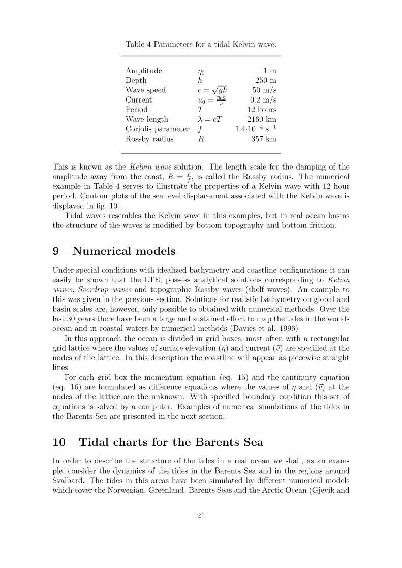
Table 4 Parameters for a tidal Kelvin wave.

Amplitude η0 1 mDepth h 250 mWave speed c =

√gh 50 m/s

Current u0 = η0g

c0.2 m/s

Period T 12 hoursWave length λ = cT 2160 kmCoriolis parameter f 1.4·10−4 s−1

Rossby radius R 357 km

This is known as the Kelvin wave solution. The length scale for the damping of theamplitude away from the coast, R = c

f, is called the Rossby radius. The numerical

example in Table 4 serves to illustrate the properties of a Kelvin wave with 12 hourperiod. Contour plots of the sea level displacement associated with the Kelvin wave isdisplayed in fig. 10.

Tidal waves resembles the Kelvin wave in this examples, but in real ocean basinsthe structure of the waves is modified by bottom topography and bottom friction.

9 Numerical models

Under special conditions with idealized bathymetry and coastline configurations it caneasily be shown that the LTE, possess analytical solutions corresponding to Kelvinwaves, Sverdrup waves and topographic Rossby waves (shelf waves). An example tothis was given in the previous section. Solutions for realistic bathymetry on global andbasin scales are, however, only possible to obtained with numerical methods. Over thelast 30 years there have been a large and sustained effort to map the tides in the worldsocean and in coastal waters by numerical methods (Davies et al. 1996)

In this approach the ocean is divided in grid boxes, most often with a rectangulargrid lattice where the values of surface elevation (η) and current (~v) are specified at thenodes of the lattice. In this description the coastline will appear as piecewise straightlines.

For each grid box the momentum equation (eq. 15) and the continuity equation(eq. 16) are formulated as difference equations where the values of η and (~v) at thenodes of the lattice are the unknown. With specified boundary condition this set ofequations is solved by a computer. Examples of numerical simulations of the tides inthe Barents Sea are presented in the next section.

10 Tidal charts for the Barents Sea

In order to describe the structure of the tides in a real ocean we shall, as an exam-ple, consider the dynamics of the tides in the Barents Sea and in the regions aroundSvalbard. The tides in this areas have been simulated by different numerical modelswhich cover the Norwegian, Greenland, Barents Seas and the Arctic Ocean (Gjevik and

21

Straume 1989, Gjevik et al. 1990, 1994, Kowalik and Proshutinsky 1995 and Lyard1997). The numerical simulations are based on numerical solutions of Laplace tidalequations with prescribed input along the boundary towards the North Atlantic andthe tide generating force on the water masses within the model domain included. Ithas been shown (Gjevik and Straume 1989) that the inflow by tidal waves from theNorth Atlantic is the most important factor for the semi-diurnal tides in the Norwegianand the Barents Seas and that the direct effect of the tide generating force within thebasin is of less importance. After harmonic analysis of the simulated time series ofsea level the results are displayed by contour maps for amplitude, Hi, and phase δi

for the various harmonic components (figs. 11-14). These type of contour maps arecommonly referred to as tidal charts. The M2 chart (fig. 11) display a characteristiccircular center with nearly vanishing sea level amplitude south-east of Svalbard. Thecontour lines for constant phase appear as spokes from the center with increasing phasevalues when one proceeds in an anticlockwise direction around the center. This type ofcontour pattern is common in tidal charts and is referred to as an amphidromic point.Two other amphidromic points of lesser extent are visible in figure 11. One in theKara Sea east of Novaja Zemlja and the other one west of Franz Josef Land. The mainamphidrome south-east of Svalbard controls the dynamics of the tide in the centralparts of the Barents Sea. It shows that a tidal wave is progressing into the BarentsSea with high amplitudes along the coast of Finnmark and with increasing amplitudeeastwards along the coasts of Kola. At the same time as the tidal wave crest passes thecoast of Finnmark the corresponding crest of the tidal wave is progressing in the deepNorwegian Sea and through the Fram Strait and into the Arctic Ocean north of Sval-bard (phase line 030). This wave is propagating around Svalbard and enter the BarentsSea in the straight between Nordaustlandet and Franz Josef Land. This wave leadsto a westward propagating wave south of Edge øya and over Svalbardbanken betweenSvalbard and Bear Island which is evident by the structure of the amphidromic point.The S2 and N2 tidal charts (figures 12 and 13) show a similar structure of contour linesas for M2 implying that these semi-diurnal tidal waves have nearly the same dynamicfeatures as M2. The tidal chart for the diurnal component K1 shows a very differentstructure particularly with the large amphidromic point in the Fram Strait betweenSvalbard and Greenland. Also the amphidromic structures south of Svalbard are morecomplex then for the semi-diurnal components with several local amplitude maximanear the shelf edge. This is a manifestation of that the diurnal tide is resonant withshelf wave modes, with nearly the same period as K1, along the pronounced shelf edgebetween northern Norway and Spitsbergen. The predictions of the model have beenvalidated by comparing with sea level and current measurements. On an average thestandard deviation between model and observations is less then 10 % (Gjevik et al.1994)

An animation of the propagating M2 tide in the Norwegian and Barents Seas canbe found on the internet site: http://www.math.uio.no/tidepred/

22

Figure 11: M2 tidal chart. Contour lines for amplitude, H , full drawn lines, phase δ, dotted lines.Units for amplitude meter, for phase degree (Greenwich). From Gjevik, Nøst and Straume, 1994

23

Figure 12: S2 Tidal chart. Contour lines for amplitude, H , full drawn lines, phase δ, dotted lines.Units for amplitude meter, for phase degree (Greenwich). From Gjevik, Nøst and Straume, 1994

24

Figure 13: N2 Tidal chart. Contour lines for amplitude, H , full drawn lines, phase δ, dotted lines.Units for amplitude meter, for phase degree (Greenwich). From Gjevik, Nøst and Straume, 1994

25

Figure 14: K1 Tidal chart. Contour lines for amplitude, H , full drawn lines, phase δ, dotted lines.Units for amplitude meter, for phase degree (Greenwich). From Gjevik, Nøst and Straume, 1994

26

11 Tidal currents

Associated with the sea level changes due to tides there are complex current fields. Inopen deep oceans the tidal current is normally small and of order 1 cm/s. Over shallowbanks and in coastal waters where the flow is constrained by topography current speedcan be of the order of 1 m/s. In narrow straits and sounds where large water masses passthrough during the tidal cycle current speed up to 3-5 m/s may occur. The Maelstrom(Moskstraumen) in Lofoten, northern Norway, is one famous example (Gjevik, Moe andOmmundsen 1997). Strong tidal currents also occur east of Spitsbergen in the FreemanSound between the Barents Island and Edge Island, in Heleysundet between the BarentsIsland and Nordaustlandet, and also in the Hinlopen Strait between Spitsbergen andNordaustlandet (Gjevik 2009).

N

~v

αE

yx

Figure 15: The tidal ellipse

The tidal currents in open sea are generally rotary i.e. the current vector rotateseither in a clockwise or a anti-clockwise fashion during the tidal cycle. At the sametime the head of the current vector describes an ellipse. With the current vector andits components denoted ~v = (u, v) the tidal ellipse can be written

(u

A)2 + (

v

B)2 = 1

where A and B are the major and minor half axis (A, B) which represent the maximumand minimum current speed respectively. The principal coordinate directions x and yare oriented along the direction of the major and minor half axis of the ellipse whichmay in general be rotated an angle α relative to local east or north (fig. 15). Thecurrent ellipse associated with the M2 component in the area south of Svalbard isshown in fig 16. Tidal currents are particularly strong over the shallow banks aroundand northeast of Bear Island. The current ellipses are here nearly circular with aclockwise rotation of the current vector. Maximum current speed is up to 1.0 m/swhich is an exceptional large current in open ocean.

Due to the effect of friction and turbulence the tidal current may vary considerablyin the vertical. Density stratification may also modify the current profile and lead to

27

Figure 16: The M2 tidal ellipses south of Svalbard. From Gjevik et al. 1990

internal wave modes (internal tides). This is particularly important in fjords (Tverberget al. 1991).

Near the critical latitude were the period of the tide coincide with the inertialperiod,it can be shown that turbulence and stratification will have a dominant effecton the profile of the tidal current. The critical latitude for the M2 component is 75o

2.8’ which passes through the Barents Sea north of Bear Island. Nøst (1994) foundthat current data from this area show the expected influence on the tidal current profilematching model predictions. Similar results from the area near the southern criticallatitude in the Wedell Sea was reported by Foldvik et al. (1990).

12 Drift and dispersion of particles in the tidal flow

In areas with strong tidal currents it represents a major factor for drift and dispersionof particles suspended in the water column. Since particles which are displaced duringthe first part of the tidal cycle may move into area with different current regime theparticles will not necessary return along the same path during the second part of thetidal cycle.Hence a net displacement or drift may occur. The tide will for examplelead to a tidal induced clockwise circulation around Bear Island where particles willcircumvent the island in 6-8 days. This has been documented both from observations(Vinje et al. 1989) and by model and laboratory studies (Straume et al. 1994, Gjeviket al. 1994, Kowalik and Proshutinsky 1995, and Gjevik 1996).

28

Figure 17: Streamlines showing strong tidal current in Ormholet near Heleysundet between Bar-entsøya and Nordaustlandet. (Photo by courtesy of Prof. Johan Ludvig Sollid).

0

60

120

180

240

300

360

10:00 16:00 22:00 04:00 10:00 16:00

10

12

14

16

18

20

22

24

26

0

10

20

30

40

50

60

10:00 16:00 22:00 04:00 10:00 16:00

10

12

14

16

18

20

22

24

26

Figure 18: Regular tidal current oscillations under sea ice near Cape Lee in the western part of theFreeman Sound. ADCP records from 10 AM on 19 April to 16 PM on 20 April 2004 (local time). Themeasurements cover from 9 to 26 meter depth. Upper graph current direction in degree true. Lowergraph current speed in cm/s. See color scale on right side. (Smedsrud and Skogseth 2004).

29

a) b)

19.0o E

74.5o N

BEARIs.

Figure 19: Observed 30 days drift of Argos buoy around Bear Island (a) (After Vinje et al., 1989).Particle trajectories in tidal current from model simulations ( 7 days) (b). (Straume et al. 1994,Gjevik 1996)

13 Mean sea level (MSL)

Mean sea level serves as a reference height or datum for tidal sea level displacementsand also for land surveying. Tidal amplitudes usually refer to MSL and the heights ofmountains and hills on maps are given relative to MSL.

Mean sea level can be determined from long records of sea level observations byeq. 12. For averaging out the effect of tidal oscillations in the records MSL is calcu-lated for a period of 19 years which covers the longest period of oscillation of the tidegenerating force from the Moon (18.6 years). MSL for this long averaging period isregularly updated and used for references. Monthly and annual mean values of MSLare also calculated and published by the national Hydrographic Services all over theworld.

Observed variation in annual mean sea level can provide information on land up-heavel or subsidence and climate changes. For example; data from Oslo, Norway(fig. 20) show a gradual lowering of mean sea level of about 30 cm over a period of85 years, corresponding to land rise of about 0.39 cm/year. This is due to the stillongoing rebound of the Earth crust after it was subpressed by the ice load during thePleictocene ice age.

Data from stations along the western and northern coast of Norway (fig. 21) showcoherent decadal variations in mean sea level. In the years 1982-83 and 1988-91 sealevel was higher then usual and this correlates to positive values of the NAO index(fig. 22). It is not unexpected that the oscillations in The North Atlantic weathersystem, as expressed by the NAO index, manifest itself by variation in mean sea levelalong the Norwegian coast. The explanation is of course that the strengthening of thewesterly wind stress over The North Atlantic and The Norwegian Sea, in period withlarge positive NAO index, leads to a transport of water towards the Norwegian coastand thereby an increase in sea level. Analysis of MSL data have become an important

30

Figure 20: Annual mean sea level (in centimeter) at Oslo for the years 1914-1999 (blue rings).

Broken red line is best regression fit corresponding to a lowering of mean sea level of 0.39 cm/year.

Figure 21: Variation in annual mean sea level (in centimeters) at four stations along the Norwegiancoast in the years 1970-1999, Oslo (red), Bergen (blue), Bodø (green) and Hammerfest (brown).

Figure 22: Difference in atmospheric pressure at sea level between Ponta Delgada at The Azores andStykkisholmur near Reykjavik on Iceland. Here expressed by the NAO-index (annual mean) for theyears 1970-1999. Positiv value of the NAO index corresponds to highest air pressure at The Azores.(From Jim Hurrell, NCAR)

31

tool for climate studies and climate modelling.An international data archive, named the Permanent Service for Mean Sea Level

(PSMSL), has therefore been established at Proudman Oceanographic Laboratory,England and MSL data from a world wide network of stations can be down loadedfrom its data base (www.pol.ac.uk/psmsl).

14 Exercises

1. Calculate the phase angle difference corresponding to a time delay of one hourfor each of the tidal components listed in table 2.

2. Find the time delay between the Moon’s transit over the Greenwich meridian andthe next high water in Longyearbyen. Consider mean high water as given by theM2 component. What will be the time delay relative to the Moon’s transit overthe local meridian through Longyearbyen?

3. At a location with predominate semi-diurnal tide the amplitude at spring is 75cm and at neap 35 cm. What are approximately the amplitude of the M2 and S2

components?

4. Assume that the tide is adequately described by only two tidal components M2

and S2. What is the exact time between neap and spring tide in this case ?

5. The minimum and maximum distance between the centers of the Moon and theEarth is about 356.500 km and 406.700 km respectively. Calculate the peak tidalacceleration in perigee and apogee position in percentage of the mean value.

6. What is approximately the time period between events with the perigee at thetime of full Moon?

7. Use the tidal tables (ref. [25]) or tidal predictions available on the internetsite http://www.asklepios.uio.no/tidepred/ to find time for high and low water(LW and HW) on 30 September 2011 at Kirkenes and Longyearbyen. Showthat the time difference for HW and LW between these two stations correspondapproximately to the phase angle difference for the M2 component.

8. Assume that sea level is responding to changes in atmospheric pressure in aquasi steady barometric fashion such that the weight of the access water columncorresponds directly to the change in atmospheric pressure. How large changes inthe atmospheric pressure (in hPa) are required to explain the difference betweenpredicted and observed sea level in fig. 8 ?

9. On basis of the tidal charts for the Barents Sea try to explain that large tidalcurrents are to be expected in the Freeman Sound between the Barents Islandand Edge Island east of Spitsbergen.

10. Use the phase information for M2 in the chart fig. 11 to estimate the averagespeed of the tidal wave along the coast of Finnmark and Kola. With the formula√

gh for the speed of long water waves find the corresponding depth. Check thedepth on maps of the area to see if this is a reasonable estimate.

32

11. The tidal current is given by its velocity components u = uo sin ωt, v = vo cos ωt ina Cartesian coordinate system x, y. uo, vo are constants ω is the angular velocityand t is time. Consider a particle which at t = 0 is located at the origin andsubsequently drifts passively with the current. Find the path or the trajectory forthe particle. What is the maximum displacement (tidal excursion) of the particlein the x and y direction respectively?

12. Suppose that we add a mean current u along the x-axis to the tidal oscillationsin problem 11. Determine the path of a particle released at the origin at t = 0and sketch the trajectory when u = uo

2and u = 2uo.

References

[1] Cartwright, E. D., (1977) Oceanic tides. Rep. Prog. Phys. 40, 665-708.

[2] Davies, M. A., J. E. Jones and J. Xing, (1996) A review of recent development intidal hydrodynamic modelling, parts I and II. J. Hydraulic Eng. ASCE , 123, No 4,278-302.

[3] Foldvik, A., J. H. Middleton and T. D. Foster (1990) Tides in the southern WedellSea. Deep Sea Res., 37, 1345-1362.

[4] Foreman, M. G. G., (1977) Manual for tidal heights analysis and predictions. Pac.Mar. Sci. Rep., 77-10, 101 pp. Inst. Ocean Sci. Sidney, B.C. Canada.

[5] Gjevik, B., and T. Straume, (1989), Model simulation of the M2 and the K1 tidein the Nordic Seas and the Arctic ocean. Tellus 41A, pp. 73–96.

[6] Gjevik, B., (1990) Model simulations of tides and shelf waves along the shelvesof the Norwegian-Greenland-Barents Seas. In: Modelling Marine Systems Ed. A.M.Davies, CRC Press Inc. Vol. I, pp. 187-219.

[7] Gjevik, B., E. Nøst, and T. Straume, (1990), Atlas of tides on the shelves of theNorwegian and the Barents Seas. Dept. of Math., Univ. of Oslo, report FoU-ST90012 to Statoil, Stavanger.

[8] Gjevik, B., E. Nøst and T. Straume, (1994), Model simulations of the tides in theBarents Sea. J. Geophysical Res., Vol 99, No C2, 3337–3350.

[9] Gjevik, B., (1996) Models of drift and dispersion in tidal flows. In Waves and Non-linear Processes in Hydrodynamics. Eds. J. Grue, B. Gjevik and J. E. Weber. KluwerAcademic Publisher, pp. 343-354.

[10] Gjevik, B., H. Moe, (1996) An interactive web site for tidal predictions in theNorwegian and Barents Seas http://asklepios.uio.no/tidepred/

[11] Gjevik, B., H. Moe og A. Ommundsen, (1997), Sources of the Maelstrom. Nature,Vol 388, 28 August 1997, 837-838.

[12] Gjevik, B., (2009) Flo og fjære langs kysten av Norge og Svalbard. Farleia Forlag.ISBN 978-82-998031-0-6.

33

[13] Kowalik, Z. and A. Yu. Proshutinsky, (1995), Topographic enhancement of tidalmotion in the western Barents Sea. J. Geophys. Res., Vol. 100, no. C2, 2613-2637.

[14] Laplace P. S. (1775) Recherches sur Quelques Points de Systeme du Monde. Mem.Acad. Roy. Sci. 88.

[15] Lyard, F. H., (1997) The tides in the Arctic Ocean from a finite element model.J. Geophys. Res., Vol. 102, no. C7, 15611-15638.

[16] Newton I. (1687) Philosophiae Naturalis Principia Mathematica, London.

[17] Nøst, E., (1994) Calculating tidal current profiles from vertically integrated modelsnear the critical latitude in the Barents Sea J. Geophys. Res., Vol. 99, no. C4,7885-7901.

[18] Pawlowicz, P., Beardsley, B., and Lentz, S. (2002) Classical tidal analysis includingerror estimated in Matlab using T-tide. Computers and Geoscience 28, 929-937.

[19] Schwiderski, E. W., (1980) On charting global ocean tides. Rev. Geophys. andSpace Physics 18, 243-268.

[20] Schwiderski, E. W., (1986) Tides. In The Nordic Seas (ed. B. G. Hurdle): NewYork Springer-Verlag, 191-209.

[21] Lars H. Smedsrud and Ragnheid Skogseth (2006) Field measurements of Arcticgrease ice properties and processes. Cold Regions Science and Technology, Vol. 44,171-183.

[22] Sato, T. et al. (2006) A geophysical interpretation of the secular displacement andgravity rates observed at Ny-Alesund, Svalbard in the Arctic– effects of post-glacialrebound and present-day ice melting. Geophysical Journal International Vol. 165,729–743.

[23] Straume. T., J. H. Nilsen,T. A McClimans, and B. Gjevik, (1994), Circulationaround Bear Island in the Barents Sea: Numerical and laboratory simulations. An-nales Geophysicae, Vol. 12 suppl. II, C 277, Abstract to EGS-General Assembly,Grenoble.

[24] Thomson, W. (lord Kelvin) (1868) Report of Committee for the Purpose of Har-monic Analysis of Tidal Observations. British Association for the Advancement ofScience, London.

[25] Tidevannstabeller for den norske kyst med Svalbard (2011), Statens Kartverk,Sjøkartverket, Stavanger. ISSN 0801-2024, 88 pp.

[26] Tverberg, V., H. Cushman-Roisin and H. Svendsen, (1991) Modeling internal tidesin fjords J. Marine Res. 49, 635-658.

[27] Vinje. T., H. Jensen, A. S. Johnsen, S. Løset, S. E. Hamran, S. M. Løvas , and B.Erlingsson, (1989), IDAP-89 R/V Lance deployment. Vol. 2; Field observations andanalysis. Norwegian Polar Research Institute, Oslo and SINTEF/NHL,Trondheim80pp.

34