lectures on advanced quantum mechanicsses/files/zirnbaueraqm.pdf · lectures on advanced quantum...
TRANSCRIPT

Lectures on Advanced Quantum Mechanics
M. ZirnbauerInstitut fur Theoretische Physik,
Universitat zu Koln
WS 2009/2010
Contents
1 Scattering theory 4
1.1 Preliminaries . . . . . . . . . . . . . . . . . . . . . . . . . . . . . . . . . . . . . . 4
1.2 Type of scattering process . . . . . . . . . . . . . . . . . . . . . . . . . . . . . . . 5
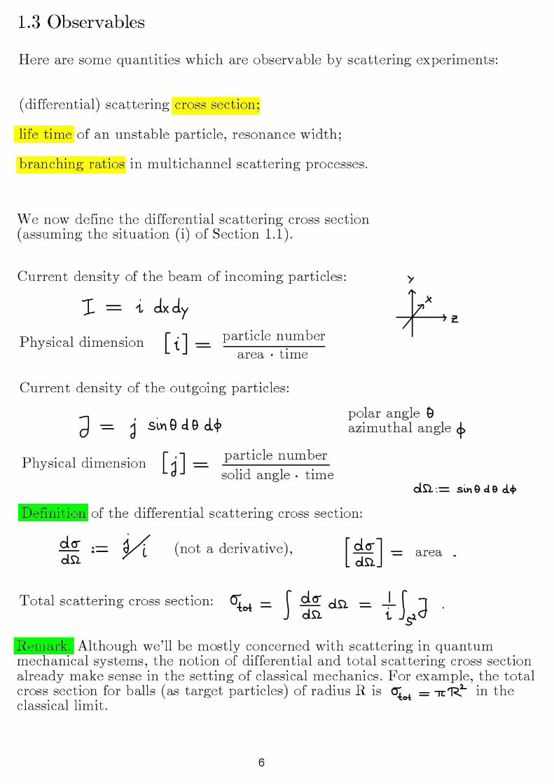
1.3 Observables . . . . . . . . . . . . . . . . . . . . . . . . . . . . . . . . . . . . . . . 6
1.4 Lippmann-Schwinger equation . . . . . . . . . . . . . . . . . . . . . . . . . . . . . 7
1.4.1 Examples . . . . . . . . . . . . . . . . . . . . . . . . . . . . . . . . . . . . 9
1.5 Scattering by a centro-symmetric potential (partial waves) . . . . . . . . . . . . . 10
1.5.1 Optical theorem . . . . . . . . . . . . . . . . . . . . . . . . . . . . . . . . . 12
1.5.2 Example: scattering from a hard ball . . . . . . . . . . . . . . . . . . . . . 13
1.5.3 Asymptotics of the spherical Bessel functions . . . . . . . . . . . . . . . . . 14
1.6 Time-dependent scattering theory . . . . . . . . . . . . . . . . . . . . . . . . . . . 16
1.6.1 Example: potential scattering d = 1 . . . . . . . . . . . . . . . . . . . . . . 18
1.6.2 Scattering by a centro-symmetric potential in d = 3 . . . . . . . . . . . . . 20
1.7 Time reversal and scattering . . . . . . . . . . . . . . . . . . . . . . . . . . . . . . 22
1.7.1 Some linear algebra . . . . . . . . . . . . . . . . . . . . . . . . . . . . . . . 25
1.7.2 T -invariant scattering for spin 0 and 1/2 . . . . . . . . . . . . . . . . . . . 27
2 Relativistic quantum mechanics: Dirac equation 28
2.1 Motivation . . . . . . . . . . . . . . . . . . . . . . . . . . . . . . . . . . . . . . . . 28
2.2 Dirac equation . . . . . . . . . . . . . . . . . . . . . . . . . . . . . . . . . . . . . 29
2.3 Relativistic formulation . . . . . . . . . . . . . . . . . . . . . . . . . . . . . . . . . 30
2.4 Non-relativistic reduction . . . . . . . . . . . . . . . . . . . . . . . . . . . . . . . . 31
2.5 Enter the electromagnetic field . . . . . . . . . . . . . . . . . . . . . . . . . . . . . 32
2.6 Continuity equation . . . . . . . . . . . . . . . . . . . . . . . . . . . . . . . . . . . 33
2.7 Clifford algebra . . . . . . . . . . . . . . . . . . . . . . . . . . . . . . . . . . . . . 35
2.8 Spinor representation . . . . . . . . . . . . . . . . . . . . . . . . . . . . . . . . . . 37
2.8.1 Tensor product . . . . . . . . . . . . . . . . . . . . . . . . . . . . . . . . . 40
1

2.9 Transforming scalar and vector fields . . . . . . . . . . . . . . . . . . . . . . . . . 41
2.10 Infinitesimal spin transformations . . . . . . . . . . . . . . . . . . . . . . . . . . . 42
2.11 Spin group . . . . . . . . . . . . . . . . . . . . . . . . . . . . . . . . . . . . . . . . 45
2.12 Relativistic covariance of the Dirac equation . . . . . . . . . . . . . . . . . . . . . 46
2.13 Discrete symmetries of the Dirac equation . . . . . . . . . . . . . . . . . . . . . . 48
2.13.1 Pin group and parity transformation . . . . . . . . . . . . . . . . . . . . . 48
2.13.2 Anti-unitary symmetries of the Dirac equation . . . . . . . . . . . . . . . . 49
2.13.3 Parity violation by the weak interaction . . . . . . . . . . . . . . . . . . . 50
2.14 Dirac electron in a Coulomb potential . . . . . . . . . . . . . . . . . . . . . . . . . 52
2.14.1 Using rotational symmetry . . . . . . . . . . . . . . . . . . . . . . . . . . . 52
2.14.2 Reduction by separation of variables . . . . . . . . . . . . . . . . . . . . . 53
2.14.3 Solution of radial problem . . . . . . . . . . . . . . . . . . . . . . . . . . . 54
3 Second quantization 57
3.1 Bosons and fermions . . . . . . . . . . . . . . . . . . . . . . . . . . . . . . . . . . 57
3.2 Weyl algebra and Clifford algebra . . . . . . . . . . . . . . . . . . . . . . . . . . . 59
3.3 Representation on Fock space . . . . . . . . . . . . . . . . . . . . . . . . . . . . . 62
3.4 Fock space scalar product . . . . . . . . . . . . . . . . . . . . . . . . . . . . . . . 65
3.5 Second quantization of one- and two-body operators . . . . . . . . . . . . . . . . . 66
3.6 Second quantization of Dirac’s theory . . . . . . . . . . . . . . . . . . . . . . . . . 69
3.6.1 Motivation: problems with the Dirac equation . . . . . . . . . . . . . . . . 69
3.6.2 Stable second quantization . . . . . . . . . . . . . . . . . . . . . . . . . . . 70
3.6.3 The idea of hole theory . . . . . . . . . . . . . . . . . . . . . . . . . . . . . 72
3.6.4 Mode expansion of the Dirac field . . . . . . . . . . . . . . . . . . . . . . . 73
3.7 Quantization of the electromagnetic field . . . . . . . . . . . . . . . . . . . . . . . 75
3.7.1 Review and consolidation . . . . . . . . . . . . . . . . . . . . . . . . . . . 75
3.7.2 More preparations . . . . . . . . . . . . . . . . . . . . . . . . . . . . . . . 77
3.7.3 Symplectic structure . . . . . . . . . . . . . . . . . . . . . . . . . . . . . . 78
3.7.4 Complex structure . . . . . . . . . . . . . . . . . . . . . . . . . . . . . . . 79
3.7.5 Fock space: multi-photon states . . . . . . . . . . . . . . . . . . . . . . . . 81
3.7.6 Casimir energy . . . . . . . . . . . . . . . . . . . . . . . . . . . . . . . . . 82
3.7.7 Mode expansion for the torus geometry . . . . . . . . . . . . . . . . . . . . 83
3.8 Matter-field interaction . . . . . . . . . . . . . . . . . . . . . . . . . . . . . . . . . 84
3.9 γ-decay of excited states . . . . . . . . . . . . . . . . . . . . . . . . . . . . . . . . 85
4 Invariants of the rotation group SO3 86
4.1 Motivation . . . . . . . . . . . . . . . . . . . . . . . . . . . . . . . . . . . . . . . . 86
4.2 Basic notions of representation theory . . . . . . . . . . . . . . . . . . . . . . . . . 86
4.2.1 Borel-Weil Theorem. . . . . . . . . . . . . . . . . . . . . . . . . . . . . . . 89
2
4.3 Invariant tensors . . . . . . . . . . . . . . . . . . . . . . . . . . . . . . . . . . . . 91
4.3.1 Invariant tensors of degree 2 . . . . . . . . . . . . . . . . . . . . . . . . . . 92
4.3.2 Example: SO3-invariant tensors of degree 2 . . . . . . . . . . . . . . . . . . 93
4.3.3 Example: SU2-invariant tensors of degree 2 . . . . . . . . . . . . . . . . . . 95
4.3.4 Invariant tensors of degree 3 . . . . . . . . . . . . . . . . . . . . . . . . . . 98
4.4 The case of SU2 : Wigner 3j-symbol, Clebsch-Gordan coefficient . . . . . . . . . . 100
4.5 Integrals of products of Wigner D-functions . . . . . . . . . . . . . . . . . . . . . 105
4.6 Tensor operators, Wigner-Eckart Theorem . . . . . . . . . . . . . . . . . . . . . . 108
5 Dirac quantization condition 109
5.1 Dirac’s argument . . . . . . . . . . . . . . . . . . . . . . . . . . . . . . . . . . . . 110
5.2 The treatment of Wu & Yang . . . . . . . . . . . . . . . . . . . . . . . . . . . . . 113
5.3 Special case: monopole charge n = 2 . . . . . . . . . . . . . . . . . . . . . . . . . 114
5.3.1 Tangent bundle . . . . . . . . . . . . . . . . . . . . . . . . . . . . . . . . . 114
5.3.2 Complex structure . . . . . . . . . . . . . . . . . . . . . . . . . . . . . . . 116
5.3.3 Covariant derivative . . . . . . . . . . . . . . . . . . . . . . . . . . . . . . 117
5.4 Other Cases (µ 6= 2h/e) . . . . . . . . . . . . . . . . . . . . . . . . . . . . . . . . 120
5.5 Lesson learned . . . . . . . . . . . . . . . . . . . . . . . . . . . . . . . . . . . . . . 122
3


1.4.1 Examples
Let us consider a few examples.
1. V (x) = V0 λ3δ(x). Here V0 has the physical dimension of energy and λ has the physical
dimension of length. δ(x) is the Dirac δ-function (actually, δ-distribution) with support at
zero (the origin of the coordinate system). The Fourier transform of the δ-function is simply
a constant, so
f(1)E (Ω) = −
m
2π~2V0λ
3 = −λ
4π
V0
~2/(2mλ2),
independent of the energy E and the outgoing direction Ω. Note that Ekin = ~2/(2mλ2) is
a rough estimate of the kinetic energy of a Schrodinger particle with mass m confined to a
box of size λ. The ratio V0/Ekin is a dimensionless measure of the strength of the scattering
potential. We have written the answer for fE in a form which makes it manifest that fE has
the physical dimension of length. We notice that the scattering amplitude fE is negative in
the repulsive case (V0 > 0) and positive in the attractive case (V0 < 0).
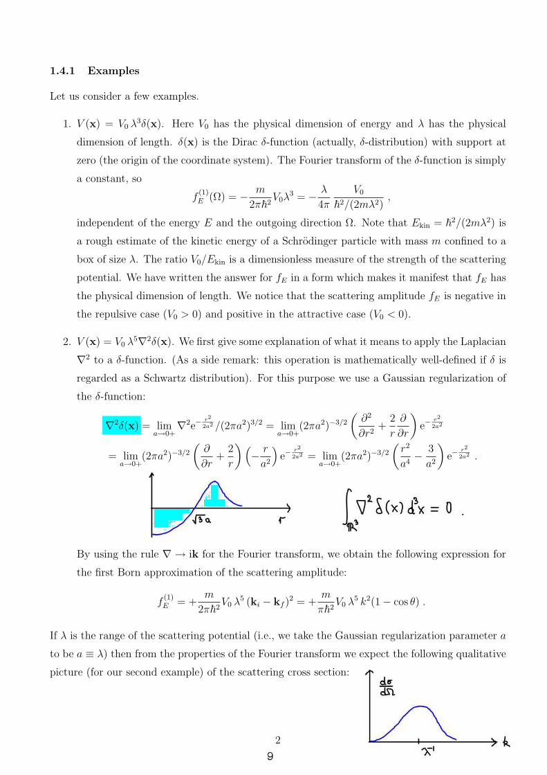
2. V (x) = V0 λ5∇
2δ(x). We first give some explanation of what it means to apply the Laplacian
∇2 to a δ-function. (As a side remark: this operation is mathematically well-defined if δ is
regarded as a Schwartz distribution). For this purpose we use a Gaussian regularization of
the δ-function:
∇2δ(x) = lim
a→0+∇
2e−r2
2a2 /(2πa2)3/2 = lim
a→0+(2πa2)−3/2
(
∂2
∂r2+
2
r
∂
∂r
)
e−r2
2a2
= lima→0+
(2πa2)−3/2
(
∂
∂r+
2
r
)
(
−r
a2
)
e−r2
2a2 = lim
a→0+(2πa2)−3/2
(
r2
a4−
3
a2
)
e−r2
2a2 .
By using the rule ∇ → ik for the Fourier transform, we obtain the following expression for
the first Born approximation of the scattering amplitude:
f(1)E = +
m
2π~2V0 λ5 (ki − kf )
2 = +m
π~2V0 λ5 k2(1 − cos θ) .
If λ is the range of the scattering potential (i.e., we take the Gaussian regularization parameter a
to be a ≡ λ) then from the properties of the Fourier transform we expect the following qualitative
picture (for our second example) of the scattering cross section:
2
1.5 Scattering by a centro-symmetric potential (partial waves)
In this section we consider Hamiltonians of the form
H = −~
2
2m∇
2 + V (r) , r =√
x2 + y2 + z2 ,
where the potential V (r) is invariant under all rotations fixing a center (which we take to be the
origin of our Cartesian coordinate system x, y, z). We assume that V (r) decreases faster than 1/r
in the limit of r → ∞.
Our goal here is to explain the ‘method of partial waves’, which is one of the standard methods
of scattering theory. To get started, we recall a few facts known from the basic course on quantum
mechanics. Using spherical polar coordinates
x = r sin θ cos φ , y = r sin θ sin φ , z = r cos θ ,
we have the following expression for the Laplacian:
∇2 =
∂2
∂x2+
∂2
∂y2+
∂2
∂z2=
1
r2
∂
∂rr2
∂
∂r+
1
r2
(
∂
sin θ
∂
∂θsin θ
∂
∂θ+
1
sin2 θ
∂2
∂φ2
)
.
If the incoming wave of the scattering wave function ψ is a plane wave eikz traveling in the z
direction, then we expect the scattering amplitude to be independent of the azimuthal angle φ
(by the rotational symmetry of the potential V ). In fact, the azimuthal angle φ will never appear
in the following discussion.
We make an ansatz for the wave function of the form
ψ =∞
∑
l=0
ψl(r) Pl(cos θ) ,
where Pl is the Legendre polynomial of degree l. We recall that Legendre polynomials are eigen-
functions of the angular part of the Laplacian:
−∂
sin θ
∂
∂θsin θ
∂
∂θPl(cos θ) = l(l + 1) Pl(cos θ) . (1.1)
We now write the energy E of the Schrodinger particle in the form E = ~2k2
2m. Our Ansatz for ψ
then leads to the following differential equation for the radial functions ψl(r) :
(
−1
r
d2
dr2 r +
l(l + 1)
r2+
2m
~2V (r)
)
ψl(r) = k2ψl(r) . (1.2)
For large values of r this equation and its general solution simplify to
−d2
dr2rψl = k2rψl , ψl(r) = A
eikr
r+ B
e−ikr
r.
Now it is a basic property (called conservation of probability or ‘unitarity’ for short) of quantum
mechanics that the divergence of the probability current density j = ~
mImψ∇ψ must vanish for
a solution ψ of the time-independent Schrodinger equation Hψ = Eψ. A quick computation
shows that div j ≡ 0 is possible only if the radially outgoing wave eikr/r and the radially incoming
10

wave e−ikr/r combine to a standing wave sin(kr + δ)/r . This requires that A and B have the
same magnitude |A| = |B|. Thus the large-r asympotics of any solution of the time-independent
Schrodinger equation Hψ = Eψ with azimuthal symmetry has to be
ψr→∞−→
∞∑
l=0
Al eikr + Bl e
−ikr
2ikr(2l + 1) Pl(cos θ) , |Al| = |Bl| . (1.3)
The factor (2l + 1)/(2ik) has been inserted for later convenience.
Our boundary conditions for the scattering problem dictate that
ψr→∞−→ eikz + fE(θ)
eikr
r.
Lemma. In order for ψ to be of this asymptotic form, the amplitudes Bl in (1.3) must be
Bl = (−1)l+1 .
To prove this lemma, we need an understanding of how eikz expands in partial waves. From
the basic quantum theory of angular momentum we recall that the Legendre polynomials have
the orthogonality property
∫ π
0
Pl(cos θ) Pl′(cos θ) sin θ dθ =2 δll′
2l + 1. (1.4)
Moreover, the Legendre polynomials form a complete system of functions on the interval [−1, +1] ∋cos θ. We may therefore expand eikz = eikr cos θ as
eikr cos θ =∞
∑
l=0
iljl(kr) (2l + 1) Pl(cos θ) , (1.5)
jl(kr) =i−l
2
∫ π
0
eikr cos θPl(cos θ) sin θ dθ . (1.6)
The factor of il has been inserted in order to make the function jl(kr) coincide with the so-called
spherical Bessel functions. The lowest-order spherical Bessel functions are
j0(ξ) =sin ξ
ξ, j1(ξ) =
sin ξ
ξ2− cos ξ
ξ.
For small values of the argument, the spherical Bessel functions behave as
jl(kr) ∼ (kr)l .
This behavior follows from the orthogonality property (1.4) of the Legendre polynomials and the
fact that any polynomial in cos θ of degree l can be expressed as a linear combination of the
Legendre polynomials Pl′(cos θ) of degree l′ ≤ l.
For large values of the argument, the spherical Bessel functions behave as
jl(kr) ≃ sin(kr − lπ/2)
kr. (1.7)
We will motivate this important relation at the end of the present subsection.
11

Proof of Lemma. Using the expansion of eikr cos θ and the large-r asymptotics of the spherical
Bessel functions we have
eikr cos θ r→∞−→∞
∑
l=0
ilsin(kr − lπ/2)
kr(2l + 1) Pl(cos θ) .
The radially incoming part for angular momentum l is given by
(
ilsin(kr − lπ/2)
kr
)
incoming
= −ile−i(kr−lπ/2)
2ikr= −eilπ e−ikr
2ikr.
Thus by comparing coefficients we obtain the desired result Bl = (−1)l+1. ¤
We now consider the difference ψ − eikz. By construction, this is a sum of radially outgoing
waves:
ψ − eikz r→∞−→∞
∑
l=0
(Al − 1)eikr
2ikr(2l + 1)Pl(cos θ) ,
which is of the expected form fE(θ)eikr/r. We already know that by unitarity we must have
|Al| = |Bl| = 1. It is customary to put Al = e2iδl and call δl the phase shift (in the channel of
angular momentum l). We then have the following result for the scattering amplitude:
fE(θ) =∞
∑
l=0
e2iδl(E) − 1
2ik(E)(2l + 1)Pl(cos θ) , (1.8)
where we have emphasized the energy dependence of the phase shift δl(E) and the wave number
k(E) =√
2mE/~ .
1.5.1 Optical theorem
We now use the formula (1.8) for the scattering amplitude fE(θ) to compute the total scattering
cross section. By the orthogonality property (1.4) of the Legendre polynomials we obtain
σtot =
∫
S2
dσ
dΩdΩ =
∫
S2
|fE(Ω)|2 dΩ =4π
k2(E)
∞∑
l=0
(2l + 1) sin2 δl(E) . (1.9)
On the other hand, since (e2iδl − 1)/(2i) = eiδl sin δl has imaginary part sin2 δl, the imaginary part
of the scattering amplitude in the forward direction is
Im fE(θ = 0) =1
k(E)
∞∑
l=0
(2l + 1) sin2 δl(E) .
Thus the total cross section and the forward scattering amplitude are related by
σtot =4π
kIm fE(0) . (1.10)
This relation is called the optical theorem.
12

1.5.2 Example: scattering from a hard ball
We now illustrate the method of partial waves at the example of scattering from a hard ball:
V (r) =
+∞ r > R ,0 r < R .
The goal is to find the scattering phase shifts δl . Having calculated these, we get the scattering
amplitude and the cross section from the formulas of the previous subsection.
The scattering wave function must vanish identically inside the ball (r < R) where the potential
is repulsive and infinite. Outside the ball (r > R) the motion is that of a free particle. The
continuity of the wave function implies Dirichlet boundary conditions at the surface of the ball:
ψ∣
∣
∣
r=R= 0 .
In the exterior of the ball, where the motion is free, we look for solutions ψl(r)Pl(cos θ) of the
Schrodinger equation for a free particle of angular momentum l . We recall that the equation for
the radial functions ψl(r) reads(
−1
r
d2
dr2 r +
l(l + 1)
r2
)
ψl(r) = k2ψl(r) . (1.11)
Solutions of this equation are the spherical Bessel functions ψl(r) = jl(kr). Indeed, we know
that the plane wave eikr cos θ is a solution of the free Schrodinger equation, and by expanding
eikr cos θ =∑
iljl(kr)(2l + 1)Pl(cos θ) and using the eigenfunction property (1.1) of the Legendre
polynomials, we that jl(kr) solves the radial equation (1.11).
Since the radial equation is of second order, a single solution is not enough to express the
most general solution. We need a linearly independent second solution. To find it, we recall
that jl(kr) ∼ rl for r ≪ k−1. Using this, it is easy to see that Ψl(x) = jl(kr)Pl(cos θ) in the
limit of r → 0 contracts to a solution of the Laplace equation ∇2ψ = 0 . Now from the chapter
on multipole expansion in electrostatics, we know that there exists a second angular momentum
l solution r−l−1Pl(cos θ) of Laplace’s equation. (Solutions of Laplace’s equation are also called
harmonic functions.) We therefore expect that there exists a solution, say nl(kr), of the radial
equation (1.11) with the corresponding small-r asymptotics:(
−1
r
d2
dr2r +
l(l + 1)
r2
)
nl(kr) = k2nl(kr) , nl(kr) ∼ r−l−1 (r → 0) . (1.12)
Such a solution nl(kr) does exist, and it is called the spherical Neumann function of degree l . The
spherical Neumann functions of lowest degree are
n0(ξ) =cos ξ
ξ, n1(ξ) = −
cos ξ
ξ2−
sin ξ
ξ.
We now make an ansatz for the wave function of free motion outside the hard ball:
ψ =∞
∑
l=0
il (al jl(kr) + bl nl(kr)) (2l + 1)Pl(cos θ) (r > R) .
13

The spherical Neumann functions have the following large-r asymptotic behavior:
nl(kr)r→∞
−→cos(kr − lπ/2)
kr.
By using also the large-r behavior of the spherical Bessel functions we find the asymptotics
ψr→∞
−→ (2ikr)−1
∞∑
l=0
(
(al + ibl)eikr
− (−1)l(al − ibl)e−ikr
)
(2l + 1)Pl(cos θ) .
Comparison with the general expression (1.3), where Al = e2iδl and Bl = −(−1)l, then yields
al + ibl = e2iδl , al − ibl = 1, and hence al = eiδl cos δl , bl = eiδl sin δl . Thus our ansatz takes the
form
ψ =∞
∑
l=0
ileiδl (cos(δl) jl(kr) + sin(δl) nl(kr)) (2l + 1)Pl(cos θ) (r > R) . (1.13)
We now impose the Dirichlet boundary condition ψ∣
∣
r=R= 0. This gives the following condition:
tan(δl) = −jl(kR)
nl(kR),
which determines the scattering phase shifts δl . This expression will be further elaborated in the
problem class.
Here we specialize to the long wave length limit kR ≪ 1 . In this limit δl ∼ (kR)2l+1. Thus
scattering is appreciable only in the s-wave channel (l = 0). The exact value of the s-wave
scattering phase shift is
δ0 = − arctan
(
j0(kR)
n0(kR)
)
= −kR .
From Eq. (1.9) we then have the total scattering cross section
σtot ≈4π
k2sin2 δl ≈ 4πR2 .
Notice that this is larger (by a factor of four) than the geometric cross section πR2 of classical
scattering from a hard ball. (There is no inconsistency in this, as the long wave length limit
kR ≪ 1 is just the opposite of the classical limit kR ≫ 1.)
1.5.3 Asymptotics of the spherical Bessel functions
Here we fill in a gap which was left in the argument above: the asymptotic behavior (1.7).
For this purpose we use the following integral representation of the Legrendre polynomials:
Pl(cos θ) =
∫ 2π
0
dφ
2π(cos θ − i sin θ cos φ)l , (1.14)
which can be verified by checking that the integral on the right-hand side satisfies the differential
equation (1.1). In combination with (1.6) this gives a representation of the spherical Bessel
functions as an integral over the unit sphere S2 :
jl(ξ) =i−l
4π
∫
S2
eiξ cos θ+l (cos θ−i sin θ cos φ) sin θ dθ dφ . (1.15)
14

For large values of ξ , the integrand oscillates strongly everywhere on S2 with the exception of two
points: the ‘north pole’ (θ = 0) and the ‘south pole’ (θ = π). These are the points where cos θ has
vanishing derivative. The contribution to the integral from each of these points can be calculated
by using the method of stationary phase (not explained here). Consider first the north pole θ = 0.
To compute its contribution to the integral, it is helpful to change coordinates as follows:
cos θ =√
1 − n21 + n2
2 , sin θ cos φ = n1 , sin θ sin φ = n2 , sin θ dθ dφ =dn1 dn2
√
1 − n21 − n2
2
.
The stationary-phase contribution to jl(ξ) from θ = 0 is then found to be
≈eiξ
4πil
∫
R2
e−iξ(n2
1+n2
2)/2dn1 dn2 =
eiξ−lπ/2
2iξ.
Similarly, the contribution from the south pole θ = π is
≈e−iξ+lπ/2
−2iξ.
By adding these two contributions, we get the claimed behavior (1.7).
15

Given a vector ψ ∈ H we look for vectors ψ± ∈ H with the approximation property
‖ Vtψ − Utψ± ‖t→±∞−→ 0 ,
i.e., evolving ψ by the full time evolution Vt for a very long time t → ±∞ leads to the same state
as evolving ψ± by the free time evolution Ut . This idea is illustrated in the figure shown below.
It should be noted, however, that it will not always be possible to find such ψ± for every ψ .
Indeed, any free motion Utψ± (if it is a free motion in the usual sense) must escape to infinity. On
the other hand, if there exist bound states and the vector ψ has nonzero projection on the space
of bound states, then Vt ψ contains a component which does not escape to infinity.
To avoid this complication, we use the unitarity of Vt (for finite t) to write
‖ Vtψ − Utψ± ‖ = ‖ ψ − V†t Utψ± ‖ .
We then postulate the existence of the following limits:
W± := limt→±∞
V†t Ut . (1.16)
The operators W± are called Moller operators, or wave operators. They are isometric, i.e., they
satisfy ‖ W±ψ ‖ = ‖ ψ ‖ for all ψ ∈ H . By the remark above they are not surjective (and hence
do not have an inverse) when bound states exist.
The definitions of Ut , Vt , and W± make sense even if the Hamiltonians H0 and/or H depend
on time. In the case of time-independent H0 and H we have the explicit formulas
Ut = e−itH0/~ , Vt = e−itH/~ , W± = limt→±∞
e+itH/~e−itH0/~ .
For the next step we require that the range of W− (i.e., the image of H under W−) be contained
in the domain of definition of W†+ :
range (W−) ⊂ domain (W †+) .
This requirement is physically reasonable, and will be discussed in Section 1.6.3 below. If it is
met, one may form the composition W†+W− . The situation is sketched in the following diagram.
16

Definition. With the pair (H0 , H) we associate an operator
S := W †+ W− , (1.17)
called the scattering operator.
Remark. The scattering operator S is unitary if domain (W †+) = range (W−). Otherwise it is an
isometry, i.e., S†S = IdH but SS† = Π projects on the orthogonal complement of the subspace of
bound states of H. For time-independent H0 , H one has the explicit formula
S = limt→∞
e+itH0/~e−2itH/~e+itH0/~ .
In the case of time-independent H0 , H the Moller operators satisfy the intertwining relations
VtW± = W±Ut . (1.18)
Heuristically, these relations are motivated by the following computation:
W±Ut = limT→±∞
V †T UT Ut = lim
T→±∞V †
T UT+t = limT→±∞
V †T−tUT = Vt lim
T→±∞V †
T UT = VtW± .
As an important corollary of the relations (1.18), the scattering operator commutes with the free
time evolution:
S Ut = Ut S . (1.19)
This is proved as follows:
S Ut = W †+W− Ut = W †
+Vt W− = (V−t W+)†W− = (W+U−t)†W− = Ut W
†+W− = Ut S .
Now by differentiating the relations (1.19) (which are valid, as we recall, in the case of time-
independent H0 , H), we deduce that the scattering operator commutes with the free Hamiltonian:
H0 S = SH0 .
From spectral theory one then knows that H0 and S can be brought to diagonal form simultane-
ously. (Note that the eigenstates of H0 usually fail to be square-integrable. Thus they do not lie
inside the Hilbert space H .)
1.6.1 Example: potential scattering d = 1
We illustrate the above at the example of potential scattering in one dimension, with
H0 = − ~2
2m
d2
dx2, H = H0 + V (x) ,
and V (x) vanishing (or decaying sufficiently fast) outside a finite region supp V ⊂ R . The
eigenspace of H0 with energy E > 0 is two-dimensional, being spanned by the two functions
φ±(x) := e±ikx , k =√
2mE/~ > 0 .
17

In order for the scattering operator S to commute with H0 , it must leave the two-dimensional
H0-eigenspace (with fixed energy E) invariant. In other words, applying S to either one of the
functions φ±(x) = e±ikx we must get a linear combination of the same two functions:
Sφ+ = ρ φ− + τ φ+ , (1.20)
Sφ− = τ ′φ− + ρ′φ+ . (1.21)
The complex numbers ρ , ρ′ (resp. τ, τ ′) are called reflection coefficients (resp. transmission coeffi-
cients). Due to S†S = IdH they satisfy the unitarity relations
|ρ|2 + |τ |2 = 1 = |ρ′|2 + |τ ′|2 , ρτ ′ + τ ρ′ = 0 = τ ′ρ + ρ′τ . (1.22)
In particular, the probabilities |ρ|2 for reflection and |τ |2 for transmission sum up to unity. We
are now left with the question of how to compute the matrix elements ρ, τ, ρ′, τ ′ of the scattering
operator. This question is answered in the sequel.
We fix an energy E = ~2k2/2m > 0 . For such an energy, we know that the eigenspace of
H0 is two-dimensional, and so is the eigenspace of H. As before, let φ±(x) = e±ikx denote the
corresponding eigenfunctions of H0 . We now introduce two sets of basis vectors for the two-
dimensional eigenspace of H with energy E. First, consider the state vectors
ψin± := W−φ± , (1.23)
obtained by applying the Moller operator W− = limt→−∞ eiHt/~e−iH0t/~ to the plane waves φ± .
These functions x 7→ ψin± (x) are solutions of the Schrodinger equation Hψin
± = Eψin± . Indeed, by
differentiating the intertwining relation (1.18) at t = 0 we obtain
HW± = W±H0 , (1.24)
which implies that if φ is an eigenfunction of H0 with energy E, then W± φ is an eigenfunction of
H (with the same energy).
Now we can say more about the solutions ψin± . Consider, e.g., ψin
+ = W−φ+. The right factor
e−itH0/~ of W− in the limit of t → −∞ sends the plane wave φ+(x) = eikx (after superposition of
a narrow range of k-values to form a localized wave packet) to x → −∞. The left factor eiHt/~
then returns the wave to the scattering region near x = 0 . This means that ψin+ is a stationary
scattering state which originates from a wave e+ikx moving in the positive x-direction and coming
in from x = −∞. In particular, ψin+ cannot have a component e−ikx at x → +∞. Thus ψin
+ must
be of the asymptotic form
ψin+ (x)
asympt−→
A · e+ikx + 0 · e−ikx x → +∞ ,1 · e+ikx + D · e−ikx x → −∞ .
Here we used the fact that scattering solutions of Hψ = Eψ become superpositions A eikx+B e−ikx
of plane waves in the limit of |x| → ∞.
18

Similarly, ψin− is a stationary scattering state which originates from a plane wave φ−(x) = e−ikx
moving in the negative x-direction and coming in from x = +∞. There cannot be any incoming
component at x → −∞, so ψin− must be of the asymptotic form
ψin− (x)
asympt−→
A′ · e+ikx + 1 · e−ikx x → +∞ ,0 · e+ikx + D′ · e−ikx x → −∞ .
One refers to ψin± as stationary scattering states satisfying incoming-wave boundary conditions.
The second set of states, ψout± , is defined by using the other Moller operator, W+ :
ψout± := W+ φ± .
It follows by inversion that
W †+ψout
± = φ± .
By the intertwining relations for W+, the states ψout± again solve the time-independent Schrodinger
equation Hψout± = Eψout
± . Called scattering states with outgoing-wave boundary conditions, they
have the asymptotics
ψout+ (x)
asympt−→
1 · e+ikx + B · e−ikx x → +∞ ,C · e+ikx + 0 · e−ikx x → −∞ ;
ψout− (x)
asympt−→
0 · e+ikx + B′ · e−ikx x → +∞ ,C ′ · e+ikx + 1 · e−ikx x → −∞ .
By comparing these asymptotic forms with those of the scattering states ψin± we directly infer that
ψin+ = Dψout
− + Aψout+ , (1.25)
ψin− = D′ψout
− + A′ψout+ . (1.26)
Finally, combining all this information we can make a statement about the scattering operator
S. By using the definition W−φ+ = ψin+ and the relations (1.25) and W †
+ψout± = φ± we compute
Sφ+ = W †+W−φ+ = W †
+ψin+ = W †
+(Dψout− + Aψout
+ ) = Dφ− + Aφ+ ,
and, similarly,
Sφ− = D′φ− + A′φ+ .
In view of Eqs. (1.20,1.21) we arrive at the identifications
D = ρ , A = τ , D′ = τ ′ , A′ = ρ′ .
19
Thus the problem of computing the matrix elements of S is reduced to finding the asymptotics of
stationary scattering states with incoming-wave boundary conditions.
Summary. If the solutions of Hψin±
= Eψin±
with incoming-wave boundary conditions are of the
asymptotic form
ψin+ −→
τ · e+ikx + 0 · e−ikx x → +∞ ,1 · e+ikx + ρ · e−ikx x → −∞ ,
ψin−
−→
ρ′ · e+ikx + 1 · e−ikx x → +∞ ,0 · e+ikx + τ ′ · e−ikx x → −∞ ,
then we have Sφ+ = ρ φ− + τφ+ and Sφ− = τ ′φ− + ρ′φ+.
1.6.2 Scattering by a centro-symmetric potential in d = 3
We return to the example (Section 1.5) of scattering by a centro-symmetric potential V = V (r)
in three dimensions. In this case the scattering operator S commutes not just with the free
Hamiltonian H0 = −~2∇2/2m but also with the square L2 of the total angular momentum and
its projection Lz on the z-axis (or any other axis):
L2 = −~
2
sin θ
∂
∂θsin θ
∂
∂θ−
~2
sin2 θ
∂2
∂φ2, Lz =
~
i
∂
∂φ.
If Ylm denotes the spherical harmonic of angular momentum l and magnetic quantum number m,
the functions
φk,l,m(r, θ, φ) = jl(kr)Ylm(θ, φ)
are joint eigenfunctions of the set of operators H0 , L2, and Lz :
H0 φk,l,m =~
2k2
2mφk,l,m , L2φk,l,m = ~
2l(l + 1) φk,l,m , Lz φk,l,m = ~mφk,l,m .
The joint eigenspace Ek,l,m with these eigenvalues is one-dimensional: Ek,l,m = C·φk,l,m . Therefore,
since S commutes with each of H0 , L2, and Lz , the function φk,l,m is an eigenfunction of S :
S φk,l,m = e2iδl(k)φk,l,m .
(In some sense, the present situation is simpler than that of d = 1, as the basis of functions φk,l,m
completely diagonalizes S.)
We now claim that the phases δl(k) are the phase shifts of Section 1.5. To verify this, we recall
that a scattering solution ψk,l,m(r, θ, ϕ) = Rk,l(r)Ylm(θ, ϕ) of the Schrodinger equation Hψk,l,m =
Eψk,l,m has the asymptotic behavior
Rk,l(r)r→∞−→ (2ikr)−1
(
e2iδl(k)ei(kr−lπ/2)− e−i(kr−lπ/2)
)
.
[Warning: we have adjusted our overall phase convention!] This solution is a solution with
incoming-wave character in the sense that its radially incoming wave component e−ikr/r is ex-
actly the same as the corresponding component of the free solution. We therefore expect that
W−φk,l,m = ψk,l,m . Indeed, the right factor of W− = limt→−∞ eitH/~e−itH0/~ sends φk,l,m (or, rather
20

a localized wave packet formed by superposition of k-values in a narrow range) to an incoming
wave e−ikr/r at r = ∞ in the distant past, and the left factor then produces the full scattering
state with a phase-shifted radially outgoing wave component (but unchanged radially incoming
wave component).
We still have to figure out what happens to ψk,l,m = W− φk,l,m when the adjoint Moller operator
W †+ is applied. We know that W †
+ψk,l,m = Sφk,l,m is a unitary number times φk,l,m , but what is
that number? To find it, we look at the radially outgoing wave component e2iδlei(kr−lπ/2)/(2ikr) of
ψk,l,m. The operator W †+ sends this component to r = ∞ by the full time evolution and then sends
it back in by the free time evolution. In this journey to infinity and back, no scattering takes
place. Therefore, whereas W− left the radially incoming wave component unchanged, it is the
radially outgoing wave component that remains unchanged under W †+. In this way, by comparing
expressions, we see that Sφk,l,m = W †+ψk,l,m = e2iδl(k)φk,l,m .
1.6.3 On the condition range(W−) ⊂ domain(W †+)
Let us make a small remark about the condition in the title of this subsection. For this we recall
from basic quantum theory that if U and V are Hilbert spaces with Hermitian scalar products
〈·, ·〉U resp. 〈·, ·〉V , then the adjoint of a linear operator A : U → V is the linear operator
A† : V → U , v 7→ A†v defined by
〈A†v, u〉U = 〈v, Au〉V
for all u ∈ U . Now if H is the Hilbert space of our problem with Hamiltonian H, let Hsc ⊂ H
denote the subspace of scattering states (i.e., the orthogonal complement of the subspace of bound
states). The adjoint of the Moller operator W+ : H → Hsc then is an operator
W †+ : Hsc → H .
In other words, domain(W †+) = range(W+) = Hsc. The condition above can therefore be reformu-
lated as
range(W−) ⊂ range(W+) . (1.27)
If the Hamiltonian H is time-reversal invariant (see the next subsection), then one can show the
identity
range(W−) = range(W+) ,
so condition (1.27) is always satisfied in that case. According to a remark made after Definition
(1.17), it follows that the scattering operator S for a time-reversal invariant system is always
unitary: S†S = IdH and SS† = IdH.
21

1.7 Time reversal and scattering
We have already mentioned the fact that unitary symmetries of the Hamiltonian (UHU−1 = H
and UH0U−1 = H0) give rise to unitary symmetries of the scattering operator (USU−1 = S).
Here we will tell a related story, describing the consequences of time-reversal symmetry (not a
unitary symmetry; see below) for scattering.
We begin with a brief discussion of time reversal in classical mechanics. In a classical phase with
position variables q and momenta p , the operation of inverting the time (called ‘time inversion’
or ‘time reversal’ for short) is the anti-canonical transformation Tcl defined by
Tcl : (q, p) 7→ (q,−p) .
It is anti-canonical because it reverses the sign of the Poisson bracket. Clearly, time reversal is an
involution, which is to say that T 2cl is the identity transformation. A classical Hamiltonian system
is called time-reversal invariant if the Hamiltonian function satisfies H = H Tcl , i.e.,
H(q, p) = H(q,−p) . (1.28)
An example of a time-reversal invariant Hamiltonian function is the kinetic energy H(q, p) =
p2/2m. For charged particles in a magnetic field B this Hamiltonian function changes to
H(q, p) =(p − eA)2
2m,
where A is a vector potential for B. We observe that in the presence of a magnetic field, time-
reversal symmetry in the sense of (1.28) is broken. (Here we take the viewpoint of regarding the
magnetic field B as ‘external’ or fixed. Time reversal continues to be a symmetry even for B 6= 0
if, along with transforming q and p , we also time-reverse B 7→ −B and A 7→ −A .)
The process of quantization is known to take canonical transformations of the classical phase
space into unitary transformations of the quantum Hilbert space, H. Now since time reversal fails
to be canonical in the classical theory, we should not expect it to be represented by a unitary
operator in the quantum theory.
Rather, time reversal in quantum mechanics will turn out to be an anti -unitary operator (the
definition is spelled out below). To motivate this fact, consider the time-dependent Schrodinger
equation (with position variables x and time variable t):
i~∂
∂tψ(x, t) = −
~2
2m∇2ψ(x, t) + V (x)ψ(x, t) .
By taking the complex conjugate on both sides and inverting the time argument, we see that if
(x, t) 7→ ψ(x, t) is a solution of this equation, then so is (x, t) 7→ ψ(x,−t). We therefore expect
that the operator T of time reversal in the position representation H = L2(R3) (and for the present
case of Schrodinger particles) is simply complex conjugation:
(Tψ)(x, t) = ψ(x, t) . (1.29)
2

This is in fact true.
Problem. Deduce from (1.29) that the time-reversal operator on wave functions ψ(p, t) in the
momentum representation is given by ψ(p, t) 7→ ψ(−p, t). ¤
We now infer two properties of the time-reversal operator T which are independent of the
representation used. The first property,
T (zψ) = z Tψ (z ∈ C , ψ ∈ H) , (1.30)
is called complex anti-linearity. It says that a complex number z goes past the time-reversal
operator T as the complex conjugate, z . Notice that this property distinguishes T from the usual
type of complex-linear operator, say A, which obeys the commutation rule Az = zA .
A stronger consequence of the formula (1.29) is that T preserves the Hermitian scalar product
〈ψ, ψ′〉 =
∫
R3
ψ(x, t) ψ′(x, t) d3x
up to complex conjugation:
∀ψ, ψ ∈ H : 〈ψ, ψ′〉 = 〈Tψ, Tψ′〉 = 〈Tψ′, Tψ〉 . (1.31)
Definition. An R-linear operator T : H → H with the property (1.31) is called anti-unitary.
Problem. (i) Show that the second property (1.31) actually implies the first property (1.30).
(ii) Show that the product of two anti-unitary operators is unitary. ¤
Next we observe that the operator T defined by (1.29) is an involution: T 2 = IdH . One may
ask whether there is a fundamental reason for T to be an involution. We will shortly see that the
answer is: no, there exists another possibility.
If an operator T acts on vectors ψ in Hilbert space by ψ 7→ Tψ , then it acts on quantum
observables A by conjugation A 7→ TA T−1. Now by the correspondence principle, the action on
observables should have a classical limit (~ → 0). Since time reversal in the classical theory is an
involution, we infer that the action A 7→ TAT−1 of time reversal on quantum observables must
also be an involution. Thus we must have
T 2AT−2 = A
for any A . This implies that T 2 = z IdH where z is some complex number. Since T 2 is unitary,
the number z = eiα must be unitary.
The possible values of the unitary number z are further constrained by associativity of the
operator product T 2 · T = T · T 2 :
z Tψ = T 2(Tψ) = T (T 2ψ) = T (zψ) = z Tψ .
It follows that our unitary number z = eiα has to be real. This leaves but two possibilities: z = 1,
and z = −1. We have already encountered a situation where z = 1. The other case of z = −1
also occurs in physics.
3

Fact. The operator of time reversal on a spinor ψ =
(ψ↑
ψ↓
)(i.e., the wave function of a particle
with spin 1/2) is realized by
(Tψ)↑(x, t) = ψ↓(x, t) , (Tψ)↓(x, t) = −ψ↑(x, t) (1.32)
in the position representation. (This fact will be explained in the chapter on Dirac theory.)
After this brief introduction to time reversal, we turn to the consequences of time-reversal
symmetry for scattering.
Definition. A quantum Hamiltonian system is called time-reversal invariant if the Hamiltonian
stays fixed under conjugation by the time reversal operator: H = THT−1. ¤
We know that the scattering operator S is obtained by taking a limit of products of time
evolution operators. Therefore, we now look at what happens to time evolution operators under
conjugation by T . By using the relations T (AB)T−1 = (TAT−1)(TBT−1), T eA T−1 = eTA T−1
and
T iT−1 = −i , we get
T e−itH/~ T−1 = e+it (THT−1)/~ ,
so for a time-reversal invariant system it follows that
T e−itH/~ T−1 = e+itH/~ =(e−itH/~
)−1.
Let now the Hamiltonian H0 for free motion be time-reversal invariant as well. Then by the
same calculation we have T e−itH0/~ T−1 =(e−itH0/~
)−1and hence
T eitH0/~ e−2itH/~ eitH0/~ T−1 =(eitH0/~ e−2itH/~ eitH0/~
)−1.
By taking the limit t → ∞ we conclude that
TST−1 = S−1. (1.33)
Corollary. Assume that H0 has no bound states and that H0 and H are time-reversal invariant.
Then the scattering operator is unitary on the full Hilbert space: S†S = SS† = IdH . (This
conclusion is not tied to time reversal but holds if the pair H0 , H has any anti-unitary symmetry.)
In concrete applications one usually looks at matrix elements of the scattering operator in
certain subspaces with fixed quantum numbers. One then wants to understand the consequences
of time-reversal invariance at the level of matrix elements. In this endeavor it is possible to get
confused. Indeed, you might make the following (incorrect) argument. You might say that since
T for spinless particles is just complex conjugation, the result (1.33) implies that the scattering
matrix is symmetric: St = S† = S−1 = T ST−1 = S. Copying from one of the standard textbooks,
you would write the scattering matrix, say for potential scattering in one dimension, as
S =
(τ ρ′
ρ τ ′
).
[You would probably argue that this, not (1.22), is the ‘correct’ way of arranging the scattering
matrix elements. After all, in the limit of vanishing potential, where we have zero reflection
4

ρ = ρ′ = 0 and full transmission, τ = τ ′ = 1, the scattering matrix should turn into the identity
matrix.] The symmetry S = St of the scattering matrix would then seem to imply that ρ?= ρ′.
This is false. The correct statement is that τ = τ ′ due to time-reversal invariance.
What went wrong with our argument? The answer is that we were not careful enough to
translate the result (1.33) for the operator S into a correct statement about the matrix of S.
Problem. Get the argument straightened out to show that τ = τ ′. ¤
In the sequel we will explain how the notion of ‘symmetry’ of the scattering operator S can be
formulated in an invariant (or basis-free) manner. For this purpose we take a time-out in order to
review some basic linear algebra.
1.7.1 Some linear algebra
Let V be a vector space over the number field K = C or K = R . We recall that the dual, V ∗,
of V is the vector space of linear functions f : V → K . Let now L : V → W be a K-linear
mapping between two K-vector spaces V and W . The canonical transpose of L is the mapping
Lt : W ∗ → V ∗ defined by
(Ltf)(v) := f(Lv) .
We call it the ‘transpose’ because, if L (resp. Lt) is expressed with respect to bases of V and W
(resp. the dual bases of V ∗ and W ∗), then the matrix of Lt is the transpose of the matrix of L.
Consider now the special case of W = V ∗. One then has W ∗ = (V ∗)∗ = V (for this, to be
precise, we should require the vector space dimension to be finite) and the canonical transpose of
L : V → V ∗ is another mapping Lt : V → V ∗ between the same vector spaces. In this situation
we can directly compare L with Lt and give a natural meaning to the word ‘symmetric’.
Definition. A linear mapping L : V → V ∗ is called symmetric if L = Lt. It is called skew if
L = −Lt.
Remark. In the case of V = W , there is no canonical definition of ‘symmetric’ linear map
L : V → V . (The matrix of L with respect to some basis of V may be symmetric, but this
property is not preserved by a change of basis in general.) To speak of a symmetric map in this
context, one needs an identification of V with V ∗, e.g., by a non-degenerate quadratic form on V .
Examples (for K = R):
1. Velocity in three-dimensional space is a vector v ∈ V ≡ R3. Momentum is not a vector (at
least not fundamentally so) but rather a form or linear function on vectors: p ∈ V ∗ = (R3)∗.
The invariant pairing p(v) :=∑
i pivi between the momentum p ∈ V ∗ and the velocity v ∈ V
of a particle has the invariant physical meaning of (twice the) kinetic energy of the particle.
The mass m (or mass tensor m in an anisotropic medium) is a symmetric linear mapping
m : V → V ∗ , v 7→ m(v) = p .
The symmetric nature of m is expressed by m(v)(v′) = p(v′) = p′(v) = m(v′)(v).
5
2. A rigid body in motion has an angular velocity ω ∈ so3 (where so3 ≃ R3 is the Lie algebra
of the rotation group SO3 fixing some point, e.g., the center of mass of the rigid body). The
angular momentum L of the body is an element L ∈ so∗3 of the dual vector space. The
pairing L(ω) computes twice the energy of rotational motion of the body. The tensor I of
the moments of inertia of the body is a symmetric linear mapping
I : so3 → so∗3 , ω 7→ I(ω) = L .
3. A homogeneous electric field E is a form E ∈ V ∗ (V = R3), while a homogeneous electric
current density j is a vector j ∈ V (or can be canonically identified with a vector once a
homogeneous charge density has been given). The invariant pairing between j and E has
the meaning of power, i.e., the rate of energy transfer between the electric field and the
matter current. The d.c. electrical conductivity σ of a metal in the Ohmic regime is a linear
mapping
σ : V ∗ → V , E 7→ σ(E) = j .
If the metal has time-reversal invariance, the conductivity is symmetric: σt = σ. If time-
reversal symmetry is broken by a magnetic field, σ acquires a skew component σH = −σtH
called the Hall conductivity. Notice that any skew (linear) mapping L : V ∗ → V for
dimV = 3 (or any other odd dimension) must have a vector e which is a null vector, i.e.,
L(e) = 0. In the case of σH this vector e coincides with the axis of the magnetic field. Since
σH(E)(E ′) = −σH(E ′)(E) = 0 vanishes for E = E ′, the Hall part of the conductivity does
not contribute to the power.
After this list of examples, we continue our review of some basic linear algebra. Let now V be
a Hermitian vector space; in other words, V is a complex vector space (K = C) equipped with a
Hermitian scalar product 〈·, ·〉V . We then have a canonical anti-linear bijection
cV : V → V ∗ , v 7→ 〈v, ·〉V . (1.34)
In the language of Dirac, this is called the ket-bra bijection, |v〉 7→ 〈v|.
Definition. Let L : V → W be a complex linear mapping between two Hermitian vector spaces
V and W . The Hermitian adjoint L† : W → V is defined as the composition
L† = c−1V Lt cW : W
cW−→ W ∗ Lt
−→ V ∗ c−1
V−→ V . (1.35)
Problem. Show that L and L† are related by the equation
〈L†w, v〉V = 〈w,Lv〉W
for all v ∈ V and w ∈ W . ¤
6
1.7.2 T -invariant scattering for spin 0 and 1/2
We are now ready to describe in what sense the scattering operator S of a time-reversal invariant
system is symmetric. Let us associate with S : H → H a complex linear operator S : H → H∗ by
S = cH T S : HS
−→ HT
−→ HcH−→ H∗ . (1.36)
Fact. The scattering operator S of a time-reversal invariant system of particles with spin zero
(resp. spin 1/2) is symmetric (resp. skew) in the sense that S = +St (resp. S = −St).
Proof. We evaluate S on a pair of vectors ψ, ψ′ ∈ H :
S(ψ)(ψ′) = 〈TSψ, ψ′〉 .
By using the relation (1.33) for a system with time-reversal invariance we obtain
〈TSψ, ψ′〉 = 〈S−1Tψ, ψ′〉 = 〈Tψ, Sψ′〉 ,
where the second equality results from the unitarity S−1 = S† of the scattering operator. In the
next step we use the anti-unitary property (1.31) of T :
〈Tψ, Sψ′〉 = 〈T 2ψ, TSψ′〉 = 〈TSψ′, T 2ψ〉 = S(ψ′)(T 2ψ) .
To summarize, writing T 2 = ǫT IdH we have
S(ψ)(ψ′) = ǫT S(ψ′)(ψ) .
Thus S is symmetric for spinless particles (ǫT = 1) and skew for spin-1/2 particles (ǫT = −1). ¤
Example. A current topic of active research are so-called topological insulators with strong spin-
orbit scattering and time-reversal invariance in d = 2 or d = 3 dimensions. The one-dimensional
boundary of such an insulator in d = 2 may house a propagating spin-1/2 mode with one right-
moving and one left-moving component. Skew symmetry constrains the scattering matrix for such
a two-component mode to be of the form
S =
(0 eiϑ
−eiϑ 0
).
This means that the reflection coefficient vanishes identically and the absolute value of the trans-
mission coefficient τ = eiϑ always remains unity as the length of the one-dimensional boundary is
increased. (Only the phase ϑ changes). Remarkably, this ‘perfectly conducting’ property of the
boundary channel is stable with respect to the introduction of any kind of (time-reversal invariant)
disorder.
7
2 Relativistic quantum mechanics: Dirac equation
2.1 Motivation
We now turn to a very fundamental theme in relativistic quantum mechanics and quantum field
theory: the Dirac equation. Its particular importance derives from the fact that all known elemen-
tary particles of matter (the so-called leptons and quarks), are described by the Dirac equation or
its quantum field-theoretic extensions. The elementary particle we have in mind here, in particular,
is the electron.
We begin our motivation with the relativistic equation relating the positive energy E of a free
particle of mass m to its momentum p :
E =√
(mc2)2 + (pc)2 . (2.1)
In attempting to reconcile quantum mechanics with special relativity, one looks for a relativistic
wave equation with the property that this relation is reproduced. By the quantum-theoretic
correspondences E ↔ i~ ∂/∂t and p ↔ ~∇/i , a first proposal for a relativistic wave equation (of
the electron, say) might be
i~∂ψ
∂t?=
√
(mc2)2 − (~c)2∇2 ψ .
It is, however, not clear how to make mathematical sense of the square root of an expression
involving the Laplacian ∇2. Defining the square root by its power series, one would end up with
a ‘non-local’ differential equation (involving derivatives up to arbitrarily high order).
To avoid the problems caused by taking a square root, an alternative approach might be to
start from the energy-momentum relation (2.1) in the squared form
E2 = (mc2)2 + (pc)2 . (2.2)
By using again the correspondences E ↔ i~ ∂/∂t and p ↔ ~∇/i one gets the wave equation
−~2 ∂2
∂t2ψ = (mc2)2ψ − (~c)2∇2ψ , (2.3)
which is known as the Klein-Gordon equation. The continuity equation naturally associated to it
is ρ + divj = 0 (leading to a conservation law∫
ρ d3x = const) with
j =~
2im
(
ψ∇ψ −∇ψ ψ)
, ρ =i~
2mc2
(
ψ ∂tψ − ∂tψ ψ)
(∂t ≡ ∂/∂t) . (2.4)
For solutions with time dependence ψ ∼ e−iωt and positive frequency ω one has ρ = ~ωmc2
|ψ|2 ≥ 0
but for ψ ∼ e+iωt the same quantity becomes negative. This means that ρ d3x in the present case,
unlike the Schrodinger case, cannot be interpreted as a probability density. (By the way: in a
quantum-field theoretic setting ρ d3x does have an interpretation as a charge density.)
It is not difficult to understand why the positivity of ρ is lacking for the Klein-Gordon equation:
it is because the expression for ρ contains the time derivative ∂t . This, in turn, is a consequence
of the Klein-Gordon equation being of second order in ∂t . (The Schrodinger equation, in contrast,
is of first order in ∂t .)
2
2.2 Dirac equation
The lesson learned from the Klein-Gordon equation is that, in trying to construct a relativistic
generalization of the Schrodinger equation, one should retain the first-order-in-∂t nature of the
equation. Special relativity then suggests that the new equation should also be of first order in
the spatial derivatives ∂/∂xj . In fact, Dirac (1928) pioneered the idea of looking for a first-order
differential operator
D = βmc2 +3
∑
j=1
αj pjc , pj =~
i
∂
∂xj
, (2.5)
with algebraic objects β, α1, α2, α3 that remain to be specified. If these satisfy the relations
β2 = 1 , βαj + αjβ = 0 , αiαj + αjαi = 2δij (i, j = 1, 2, 3) , (2.6)
then D squares to
D2 = (mc2)2 − (~c)2∇2 , ∇2 =3
∑
j=1
∂2
∂x2j
. (2.7)
Moreover, if ψ is any solution of the equation
i~∂ψ
∂t= Dψ , (2.8)
then ψ by iteration is also a solution of the equation
−~2∂2ψ
∂t2= D2ψ . (2.9)
By using the formula (2.7) for D2 we see that the latter is nothing but the Klein-Gordon equation
(2.3). Thus for plane wave solutions ψ of (2.8) with frequency ω = E/~ and wave vector k = p/~
one gets the desired energy-momentum relation (2.1). (At the same time, one gets expressions for
ρ and j of a more desirable form; see below.)
The question now is whether one can realize the algebraic relations (2.6), and if so, how. It
is certainly impossible to satisfy these relations while clinging to the Schrodinger viewpoint of
complex numbers β, . . . , α3 multiplying a wave function ψ with values in C.
Therefore, following Dirac we now abandon the Schrodinger viewpoint and allow that ψ may
take values in a more general vector space, say Cn with n ≥ 1. With that generalization, we can
take β, . . . , α3 to be n × n matrices multiplying the n-component vector ψ. It then turns out to
be possible to realize the relations (2.6) for n ≥ 4. Indeed, one possible choice for n = 4 is
β =
(
1 00 −1
)
, αj =
(
0 σj
σj 0
)
, j = 1, 2, 3, (2.10)
where 1 ≡ 12 is the 2 × 2 unit matrix and σj are the Pauli matrices:
σ1 =
(
0 11 0
)
, σ2 =
(
0 −ii 0
)
, σ3 =
(
1 00 −1
)
.
Problem. Check that the choice (2.10) satisfies the relations (2.6). ¤
3

We will elaborate on the theoretical background behind the relations (2.6) in a later subsection.
For now, we record that there exists at least one possible realization for n = 4. In our further
arguments, we will often refer to this realization for concreteness.
Definition. The Dirac equation for a free particle of mass m reads
i~∂ψ
∂t= mc2βψ +
~c
i
3∑
j=1
αj∂ψ
∂xj
, (2.11)
where ψ(x, t) takes values in C4 and the 4 × 4 matrices β, α1, α2, α3 are subject to (2.6).
2.3 Relativistic formulation
For some purposes it is useful to write the Dirac equation in a form which puts space and time
on a similar footing. The standard physics convention is to introduce
x0 := ct , xj := xj , γ0 := β, γj := βαj = −αjβ (j = 1, 2, 3) . (2.12)
With these conventions, the Dirac equation (2.11) takes the relativistic form
(
γ0 ∂
∂x0+
∑3
j=1γj ∂
∂xj+ i
mc
~
)
ψ = 0 . (2.13)
The parameter mc/~ has the physical dimension of an inverse length. Its reciprocal ~/(mc) is
called the (reduced) Compton wave length. For the electron with mass m ≈ 0.5 MeV/c2 one has
~
mc=
~c
mc2≈ 200 MeV · fm
0.5 MeV≈ 400 × 10−15m . (2.14)
In the jargon on of physics the matrices γ0, . . . , γ3 are called the gamma matrices. We note that
for the choice (2.10) they have the expressions
γ0 =
(
1 00 −1
)
, γj =
(
0 σj
−σj 0
)
, j = 1, 2, 3. (2.15)
It is customary to use Greek letters for space-time indices; i.e., µ = 0, 1, 2, 3.
Problem. Adopting this notation, show that the algebraic relations (2.6) take the concise form
γµγν + γνγµ = 2gµν1 , (2.16)
where 1 ≡ 14 is the 4 × 4 unit matrix, and
g00 = 1 , g11 = g22 = g33 = −1 , gµν = 0 for µ 6= ν , (2.17)
are the components of the Minkowski metric tensor. ¤
It is also customary in the present context to use Einstein summation convention, which says
that repeated Greek indices are understood to be summed over.
Summary. The relativistic (or covariant) form of the free-particle Dirac equation (2.11) is
(
γµ ∂
∂xµ+ i
mc
~
)
ψ = 0 . (2.18)
4

2.4 Non-relativistic reduction
Dirac’s theory is intended to be a relativistic quantum theory of the electron. We already have
a non-relativistic quantum theory of the electron, namely the Schrodinger equation or, including
spin, the Pauli equation. By the principles of theory building, in order for a new theory to be
acceptable it must be consistent with the old theory which is already known to be true (within its
limits of validity). Therefore the logical step to be taken next is to verify that the Dirac equation
reduces to the Schrodinger/Pauli equation in the non-relativistic limit.
For this purpose we write the Dirac equation in the following block-decomposed form:
0 =
(
imc~
+ 1c
∂∂t
∑
σj∂
∂xj
−∑
σj∂
∂xjimc
~− 1
c∂∂t
)
(
ψ+
ψ−
)
, ψ± =
(
ψ±,↑
ψ±,↓
)
. (2.19)
At present, the symbols ↑ and ↓ are just some fancy notation to label the two components of
ψ±(x, t) ∈ C2. (Later we will see that they do, in fact, reflect the spin of the electron.)
The non-relativistic limit is |v| ≪ c , or |k| ≪ mc/~ . By the correspondence k ↔ ∇/i
this means that the off-diagonal blocks of the matrix in (2.19) are to be considered as being much
smaller than the diagonal blocks. In zeroth-order approximation we neglect the off-diagonal blocks
altogether to obtain(
imc
~+
1
c
∂
∂t
)
ψ(0)+ = 0 , ψ
(0)− = 0 . (2.20)
We are setting ψ(0)− = 0 by fiat because we intend to identify ψ+ with the spinor wave function of
the Pauli equation, and there is no room for additional degrees of freedom in the non-relativistic
limit. (We will learn later that ψ− describes the positron, the antiparticle of the electron. In the
present context, we envisage a situation with no positrons present. Hence our choice ψ(0)− = 0.)
Note that the first equation in (2.20) implies that ψ(0)+ has the time dependence
ψ(0)+ ∼ e−imc2t/~ .
We now turn to a first-order (or improved) approximation. For this we write the system of
equations (2.19) in the form(
A BC D
) (
ψ+
ψ−
)
= 0 ,
or equivalently,
Aψ+ + Bψ− = 0 , Cψ+ + Dψ− = 0 .
We will see that the operator D = imc~− 1
c∂∂t
has an inverse when acting on Cψ+ . We can therefore
solve the second equation for ψ− , and by inserting the solution ψ− = −D−1Cψ+ into the first
equation we obtain an equation solely for ψ+ :
(A − BD−1C) ψ+ = 0 ,
or explicitly,
(
imc
~+
1
c
∂
∂t
)
ψ+ +
(
∑
σj∂
∂xj
)(
imc
~− 1
c
∂
∂t
)−1 (
∑
σj∂
∂xj
)
ψ+ = 0 .
5

Now since we know from the zeroth-order approximation that ψ+ has the leading time dependence
ψ(0)+ ∼ e−imc2t/~, we have −1
c∂∂t
ψ+ ≈ imc~
ψ+ , and we may replace −D−1Cψ+ by
−D−1Cψ+ =
(
imc
~− 1
c
∂
∂t
)−1 (
∑
σj∂
∂xj
)
ψ+ → ~
2imc
(
∑
σj∂
∂xj
)
ψ+ .
By multiplying the equation for ψ+ by i~c and slightly rearranging the terms, we then arrive at
the improved approximation ψ+ ≈ ψ(1)+ where ψ
(1)+ satisfies
i~∂ψ
(1)+
∂t= mc2ψ
(1)+ − ~
2
2m
(
∑
σj∂
∂xj
)2
ψ(1)+ .
In the final step we use the relations σjσl + σlσj = 2δjl for the Pauli matrices to find
(
∑
σj∂
∂xj
)2
=∑ ∂2
∂x2j
= ∇2 .
Altogether we have
i~∂
∂tψ
(1)+ = mc2ψ
(1)+ − ~
2
2m∇2ψ
(1)+ . (2.21)
This is indeed the free-particle Schrodinger equation with a constant shift of the energy by the
rest mass mc2. Thus the Dirac equation has passed its first test.
Note added. At the same level of approximation, the equation ψ− = −D−1Cψ+ yields
ψ(1)− =
~
2imc
(
∑
σj∂
∂xj
)
ψ(1)+ .
Thus ψ(1)− is smaller than ψ
(1)+ by, roughly speaking, a factor of ~|k|/mc or |v|/c .
2.5 Enter the electromagnetic field
In order to turn the free-particle Dirac equation (2.18) into an equation for charged particles such
as the electron, we need to introduce the coupling to the electromagnetic field. [Recall from the
course on classical electrodynamics that the electromagnetic field strength tensor, also known as
the Faraday tensor, is given by
Fµν =∂Aν
∂xµ− ∂Aµ
∂xν, (2.22)
where Aµ are the components of the 4-vector of the electromagnetic gauge field.] The form of this
coupling is determined by the principles of gauge invariance and minimal substitution, as follows.
If χ is some space-time dependent function (of physical dimension action/charge), the Faraday
tensor is invariant under gauge transformations
Aµ → Aµ +∂
∂xµχ . (2.23)
The principle of gauge invariance now says the following. If ψ is the wave function of a quantum
particle with electric charge e, then the physics of the coupled system (i.e., the particle interacting
with the electromagnetic field) must be invariant under the gauge transformation (2.23) of the
gauge field in combination with the gauge transformation
ψ → eie χ/~ψ . (2.24)
6

of the matter field ψ . It is easy to see that the expression(
~
i
∂
∂xµ− eAµ
)
ψ
is gauge invariant in this sense. The principle of minimal substitution then tells us to enforce
gauge invariance by making in the Dirac equation (or any other charged quantum wave equation,
for that matter) the substitution
∂
∂xµψ →
(
∂
∂xµ−
ie
~Aµ
)
ψ . (2.25)
Doing so, we arrive at the final form of the Dirac equation.
Definition. The Dirac equation for a particle of mass m and charge e in the presence of an
electromagnetic field (described by the gauge field Aµ) is
γµ
(
∂
∂xµ−
ie
~Aµ
)
ψ + imc
~ψ = 0 . (2.26)
Problem. By following the steps of Section 2.4, show that the full Dirac equation (2.26) in the
non-relativistic limit reduces to the Pauli equation (i.e., the Schrodinger equation including the
Pauli coupling of the spin of the charged particle to the magnetic field B):
i~∂
∂tψ
(1)+ = (mc2 + eΦ)ψ
(1)+ −
~2
2m
∑
j
(
∂
∂xj
−ie
~Aj
)2
ψ(1)+ −
e~
m
∑
j
Bj σjψ(1)+ . (2.27)
Here Φ = −cA0 is the electric scalar potential, and Aj are components of the magnetic vector
potential A obeying curlA = B . ¤
2.6 Continuity equation
At this stage of the theoretical development, one might hope that the probabilistic interpretation of
the square |ψ|2 of the Schrodinger wave function could be carried over without any essential change
to the Dirac equation (as a single-particle theory). In the present subsection we substantiate this
optimistic thought. Later, however, we will see that there are serious problems with this inter-
pretation, and we will indicate what needs to be changed to end up with a satisfactory theory.
The probabilistic interpretation of the Schrodinger wave function |ψ|2 =: ρ rests on the continu-
ity equation ρ + div j = 0 together with positivity, ρ ≥ 0 . Let us now transcribe the Schrodinger
derivation of this equation (which students know from basic quantum mechanics) to the Dirac
case. For this purpose we start from the Dirac equation (2.26) in the form
(
∂
∂t+
ie
~Φ
)
ψ + c∑
(
∂
∂xl
−ie
~Al
)
αlψ + imc2
~βψ = 0 . (2.28)
ψ has four components, as we recall, and thus takes values in C4. We now assume that the vector
space C4 is Hermitian, i.e., is equipped with a Hermitian scalar product C
4 ×C4 → C . Using this
structure we define the Hermitian adjoint ψ† with values in the dual vector space (C4)∗, and ψ†ψ
with values in C (actually, R).
7

Now observe that the matrices β and αl in (2.10) are Hermitian: β = β† and αl = α†l
(l = 1, 2, 3). We promote this observation to an axiom of the theory, i.e., we demand that any
permissible choice of β and αl must not only obey the algebraic relations (2.6) but must also have
the property of being Hermitian. By dualizing the equation (2.28) we then obtain the following
equation for ψ† :
(
∂
∂t− ie
~Φ
)
ψ† + c∑
(
∂
∂xl
+ie
~Al
)
ψ†αl − imc2
~ψ†β = 0 . (2.29)
Next we contract the equation (2.28) for the vector ψ with the dual vector ψ†, and similarly the
equation (2.29) for ψ† with ψ . Afterwards we add the two resulting scalar equations. The terms
containing i =√−1 all cancel since their signs are changed by taking the Hermitian adjoint. So
we get∂
∂tψ†ψ + c
∑
l
∂
∂xl
ψ†αlψ = 0 . (2.30)
This has the form of a continuity equation ρ + div j = 0 if we let
ρ := ψ†ψ , jl := c ψ†αlψ . (2.31)
Summary. We record that if ψ is a solution of the Dirac equation (with or without electromag-
netic field), then the scalar ρ = ψ†ψ and the vector j with components jl = c ψ†αlψ satisfy the
continuity equation
ρ + div j = 0 . (2.32)
By a standard argument using the divergence theorem (a.k.a. Gauss’ theorem) it follows that the
total space integral∫
ρ d3x is conserved.
Remark. Coming from Schrodinger quantum mechanics, it is natural to think that ρ (actually,
ρ d3x) is the probability density for a relativistic electron, and j is the vector of the corresponding
probability current density. However, it will turn out that this (wishful) thinking is untenable.
Dirac’s theory in fact will have to be reformulated (in the framework of quantum field theory)
so as to give ρ the interpretation of charge density of the electron (actually of the quantum field
encompassing the electron as well as the positron).
8

2.7 Clifford algebra
In this and the following subsection we provide some theoretical background concerning the four-
component nature of the wave function ψ of the Dirac equation. A question which was left open
in Section 2.3 is this: how can we say a priori that the algebraic relations
γνγν + γνγµ = 2gµν
are realizable for n×n matrices with n ≥ 4 , and how can such a matrix realization be constructed?
To answer this question, we shall take the liberty of going into more detail than is offered in most
physics textbooks, as the very same formalism will turn out to be relevant for the procedure of
second quantization of many-particle quantum mechanics.
In the sequel we will be concerned with a vector space V over the real number field K = R
or the complex number field K = C . We assume that V comes with a non-degenerate symmetric
K-bilinear form (also referred to as a ‘quadratic form’ for short)
Q : V × V → K , (v, v′) 7→ Q(v, v′) = Q(v′, v) . (2.1)
Examples. We give two examples, the number field being K = R in both cases. The first example
is the Euclidean vector space V = R3 equipped with the Euclidean scalar product Q,
Q(v, v′) = |v| |v′| cos ∠(v, v′) .
The second example is the example of relevance for the Dirac equation: the Lorentzian vector
space V = R4 with the Minkowski scalar product Q given by (summation convention!)
Q(v, w) = Q (vµeµ , wνeν) = gµν vµwν = v0w0 − v1w1 − v2w2 − v3w3 (2.2)
in any standard basis e0, e1, e2, e3. ¤
To define what is meant by the Clifford algebra of a vector space V with quadratic form Q,
we need the following basic concept.
Definition. An associative algebra is a vector space, say A , with the additional structure of an
associative product A×A → A , (a, b) 7→ ab, which distributes over addition: a(b + c) = ab + ac.
Remark. As usual, associativity of the product means that there is no need to use parentheses
in multiple products such as abc = (ab)c = a(bc). The main examples for an associative algebra
are provided by matrices: the K-vector space of matrices of size n×n (say) with matrix elements
taken from K , is an associative algebra with the product being the usual matrix multiplication.
Definition. The Clifford algebra Cl(V,Q) of the vector space V with quadratic form Q is the
associative algebra generated by V ⊕ K with relations
vw + wv = 2Q(v, w) . (2.3)
2

Remark. The words ‘associative algebra generated by V ⊕K’ mean that the elements of Cl(V,Q)
are polynomial expressions in the elements of V with coefficients taken from the number field K .
The relations (2.3) imply, e.g.,
uvw = uwv − 2Q(v, w)u = vuw − 2Q(u, v)w (u, v, w ∈ V ) .
Example. Let (V = R4, Q) be the Lorentzian vector space with Minkowski scalar product Q.
Take e0, e1, e2, e3 to be some standard basis of V , so that Q(eµ , eν) = gµν where g00 = −g11 =
−g22 = −g33 = 1. Then some examples of elements in Cl(V,Q) are
e0e0 = 1 , e1e1 = −1 , e0e1 = −e1e0 , e0e1e0 = −e1 .
All this may seem abstract and unfamiliar. It can be made more tangible as follows.
Let us think of the vectors e0 , . . . , e3 as basis elements in some four-dimensional subspace
V ≃ R4 of the linear space (or vector space) of 4 × 4 matrices with quadratic form
Q(v, v′) = 14Tr (vv′) . (2.4)
More precisely, let
e0 =
(
1 00 −1
)
, ej =
(
0 −σj
σj 0
)
(j = 1, 2, 3) .
One easily verifies the scalar products Q(eµ, eν) = gµν . Thus V ≃ R4 becomes the four-dimensional
real vector space of matrices of the form
v =
v0 0 −v3 −v1 + iv2
0 v0 −v1 − iv2 v3
v3 v1 − iv2 −v0 0v1 + iv2 −v3 0 −v0
. (2.5)
Because we have realized our vectors v = vµeµ as matrices, the vector space V ≃ R4 now carries
the additional structure of an associative algebra with matrix multiplication playing the role of
the product. If Id denotes the 4 × 4 unit matrix, one sees that the relations
vw + wv = 2Q(v, w) Id (2.6)
are satisfied by the matrices (2.5).
Thus, in the present example Cl(V, Q) can be realized as the algebra of 4×4 matrices that arise
by multiplication of generators of the form (2.5). Using mathematical language one calls such a
concrete realization by matrices a representation of the abstractly defined algebra. Essentially the
same representation was given in an earlier subsection [with only a minor sign difference due to
the relativistic convention of raising and lowering indices]. ¤
Problem. Show that if dim V = n and e1, . . . , en is a Q-orthogonal basis of V , then the
following Clifford algebra elements constitute a basis of Cl(V, Q) as a vector space:
1 , ej (j = 1, . . . , n) , eiej (i < j) , eiejel (i < j < l) , . . . , e0e1 · · · en . (2.7)
Count the number of these elements to deduce that dim Cl(V,Q) = 2 dim V .
3
2.8 Spinor representation
While the Clifford algebra Cl(V, Q) is defined abstractly as an associative algebra with certain
binary relations, we saw that Cl(V,Q) has a concrete realization by 4×4 matrices for the Minkowski
example of V = R4. This realization will be called the spinor representation of Cl(R4, Q) from
now on. In Section 2.7 we simply wrote down the spinor representation without explaining where
it came from. This gap in our theoretical development is to be closed in the present subsection.
For brevity we will only consider the special case of a real vector space V ≃ R2n of even
dimension with Euclidean scalar product Q. Given this situation, let us fix some orthonormal
basis e1, . . . , en, f1, . . . , fn of V .
Although everything so far is real (K = R), we are now going to consider complex linear
combinations of the vectors v ∈ V ; mathematically speaking we pass to the complexification
V ⊗R C of V . (The symbol ⊗K denotes the tensor product of vector spaces over K ; see the end
of this subsection for a quick exposition.) In the complexification V ⊗R C we then form the linear
combinations (i =√−1 )
cj := (ej − ifj)/2 , c∗j := (ej + ifj)/2 (j = 1, . . . , n) . (2.8)
We also introduce the complex vector spaces
P = spanCc1, . . . , cn , P ∗ = spanCc∗1, . . . , c∗n , (2.9)
and record the decomposition
V ⊗R C = P ⊕ P ∗ . (2.10)
Such a decomposition is called a polarization. [The notation indicates that P ∗ may be regarded
as the dual vector space of P via the non-degenerate pairing P ⊗ P ∗ → C by (c, c∗) 7→ Q(c, c∗).]
Notice that the Clifford relations (2.3) imply the following relations for our new generators:
cjcl + clcj = 0 , c∗jc∗
l + c∗l c∗
j = 0 , cjc∗
l + c∗l cj = δjl (j, l = 1, . . . , n) . (2.11)
In physics, these relations are called the canonical anti-commutation relations (CAR). They will
play a central role in the formalism of second quantization for many-fermion systems.
To formulate the algorithm for constructing the spinor representation of Cl(V,Q), we need one
more algebraic concept.
Definition. By the exterior algebra ∧(U) of a K-vector space U one means the associative algebra
generated by U ⊕ K with relations
∀u, u′ ∈ U : uu′ + u′u = 0 . (2.12)
The exterior algebra is a direct sum of subspaces of fixed degree:
∧(U) =dim U⊕
l=0
∧l(U) , (2.13)
4

where ∧0(U) ≡ K , ∧1(U) ≡ U , ∧2(U) consists of all quadratic elements∑
uiuj , ∧3(U) consists
of all cubic elements∑
uiujuk , and so on.
Remarks. i) Note that (2.12) implies u2 = 0 for any u ∈ U ⊂ ∧(U). ii) In physics the exterior
algebra ∧(U) is also known as the fermionic Fock space of U . (More precisely, if U is a Hilbert
space, then ∧(U) is another Hilbert space called the fermionic Fock space associated to the single-
particle Hilbert space U .) In the Fock space setting the degree has the physical meaning of particle
number. iii) The notion of exterior algebra is basic to the calculus of differential forms.
Problem. Show that the exterior algebra ∧(U) is isomorphic as a vector space to the Clifford
algebra Cl(U,Q). Hint: prove by construction of a basis that ∧(U) has dimension 2 dim U . ¤
We now recall the definition of the complex vector space P ∗ in (2.9) and make the important
observation that the exterior algebra of P ∗ (or P for that matter) is contained as a subalgebra in
Cl(V, Q)⊗C . By this observation the exterior algebra ∧(P ∗) can be turned into a representation
space for Cl(V, Q) as follows.
We are looking for an operation of Cl(V,Q) on ∧(P ∗),
Cl(V, Q) × ∧(P ∗) → ∧(P ∗) , (a, ξ) 7→ a · ξ , (2.14)
which is a representation. In other words, we want a Clifford multiplication rule (2.14) which is
compatible with the associative product in the Clifford algebra in the sense that (i) the relation
(ab) · ξ = a · (b · ξ) (2.15)
holds for all a, b ∈ Cl(V, Q), ξ ∈ ∧(P ∗), and (ii) the Clifford relations (2.3) are preserved, i.e., for
all v, w ∈ V ⊂ Cl(V,Q), ξ ∈ ∧(P ∗), we have
v · (w · ξ) + w · (v · ξ) − 2Q(v, w) · ξ = 0 . (2.16)
Since Cl(V, Q) is generated by V ⊕ K it is sufficient to specify the Clifford multiplication (2.14)
for scalars k ∈ C ⊂ Cl(V, Q) and vectors v ∈ V ⊂ Cl(V,Q). In the former case the multiplication
(2.14) is the natural one and needs no explanation.
In order to describe the multiplication by vectors v ∈ V (in the following we use the alternative
word ‘action’ for it) we use the polarization V ⊗R C = P ⊕ P ∗. First, let v ∈ P ∗. The action of
such an element v ∈ P ∗ on ξ ∈ ∧(P ∗) is simply exterior multiplication:
v · ξ := vξ , (2.17)
i.e., the product is computed in the exterior algebra ∧(P ∗). Note that the action of v ∈ P ∗
increases the degree: it maps ∧l(P ∗) into ∧l+1(P ∗).
Second, let v ∈ P . Such elements act by an operation which lowers the degree:
P ∋ v : ∧l(P ∗) → ∧l−1(P ∗) . (2.18)
5

This operation is defined recursively. For the two lowest degrees l = 0, 1 one sets
l = 0 : v · 1 := 0 , (2.19)
l = 1 : v · v′ := 2Q(v, v′) . (2.20)
The action on higher-degree elements is then defined by the so-called anti-Leibniz rule:
v · (ξη) := (v · ξ) η + (−1)lξ (v · η) , ξ ∈ ∧l(P ∗). (2.21)
Claim. Equations (2.17)–(2.21) give a representation of Cl(V, Q) on ∧(P ∗). ¤
Since all elements of V ⊕ K ⊂ Cl(V, Q) act as linear operators and multiplication of linear
operators is associative, it is immediately clear that the compatibility condition (2.15) is satisfied.
To verify the Claim, what must be shown is that the property (2.16) holds. For this purpose we
introduce some more notation. We write the decomposition of v ∈ V by V ⊗R C = P ⊕ P ∗ as
v = vP + vP ∗ . We then denote the degree-increasing action of the P ∗-component vP ∗ by ε(vP ∗)
and the degree-lowering operation of the P -component vP as ι(vP ). [In physics one calls ε(vP ∗)
the particle creation component and ι(vP ) the particle annihilation component of v.] Thus
v · ξ = ε(vP ∗)ξ + ι(vP )ξ . (2.22)
Problem. Show that the anti-commutation relations
ε(x)ε(x′) + ε(x′)ε(x) = 0 , ι(y)ι(y′) + ι(y′)ι(y) = 0 ,
ε(x)ι(y) + ι(y)ε(x) = 2Q(x, y) Id∧(P ∗) (2.23)
hold for all x, x′ ∈ P ∗ and y, y′ ∈ P . ¤
Using the result (2.23) we do the following calculation:
v · (w · ξ) + w · (v · ξ) − 2Q(v, w) · ξ
=(
ε(vP ∗) + ι(vP ))(
ε(wP ∗) + ι(wP ))
ξ +(
ε(wP ∗) + ι(wP ))(
ε(vP ∗) + ι(vP ))
ξ − 2Q(v, w)ξ
= ε(vP ∗)ι(wP )ξ + ι(wP )ε(vP ∗)ξ + ε(wP ∗)ι(vP )ξ + ι(vP )ε(wP ∗)ξ − 2Q(v, w)ξ
= 2Q(vP ∗ , wP )ξ + 2Q(vP , wP ∗)ξ − 2Q(v, w)ξ = 0 .
Thus the condition (2.16) and is indeed satisfied and our Claim is true. What we have learned is
summarized in the next statement — where we keep the assumption of even dimension of V but
drop the (unnecessary) condition that Q be a Euclidean structure.
Definition. Let (V, Q) be an even-dimensional vector space over the reals R with polarization
V ⊗R C = P ⊕ P ∗. The spinor representation of the Clifford algebra Cl(V, Q) is defined to be the
representation on the exterior algebra ∧(P ∗) which is given by the action (2.22). ¤
It is now straightforward to produce a matrix representation of Cl(V,Q) by fixing a basis of
∧(P ∗) and expanding the action of the Clifford algebra elements w.r.t. this basis.
6

Example. We illustrate the procedure at the simple example of the Euclidean plane V = R2
with orthonormal basis e, f. As before, let c := (e − if)/2 and c∗ := (e + if)/2. The action of
c∗ and c on the basis 1, c∗ of ∧(P ∗) is computed to be
c∗ · 1 ≡ ε(c∗)1 = c∗ , c∗ · c∗ ≡ ε(c∗)c∗ = (c∗)2 = 0 ,
and
c · 1 ≡ ι(c)1 = 0 , c · c∗ ≡ ι(c)c∗ = 2Q(c, c∗) = 12Q(e − if, e + if) = 1 .
Thus if we make the following identifications for the basis vectors 1, c∗ of ∧(P ∗):
1 ≡(
01
)
, c∗ ≡(
10
)
,
then the Clifford algebra elements 1, e, f , and ef are represented by the matrices
matrix(1) =
(
1 00 1
)
,
matrix(e) = matrix(c + c∗) =
(
0 11 0
)
= σ1 ,
matrix(f) = matrix(ic − ic∗) =
(
0 −ii 0
)
= σ2 ,
matrix(ef) =
(
i 00 −i
)
= iσ3 .
Problem. By following the same procedure, construct the spinor representation of the Clifford
algebra Cl(V,Q) for the Euclidean vector space V = R4 with orthonormal basis e1, e2, f1, f2. ¤
We finish this subsection with a few final comments:
1. The same construction applied to the Lorentzian vector space V = R4 with Minkowski scalar
product gives the so-called Weyl form of the gamma matrices:
γ0 =
(
0 1
1 0
)
, γj =
(
0 σj
−σj 0
)
(j = 1, 2, 3). (2.24)
2. The spinor representation of Cl(R2n, Q) is the one and only representation of Cl(R2n, Q)
which is both non-trivial and irreducible.
3. We recall the dimension formulas dim Cl(V, Q) = 2dim V and dim ∧ (P ∗) = 21
2dim V . For the
case of four dimensions (V = R4) it so happens that the dimension 2
1
2dim V = 22 of the spinor
representation is also four. This coincidence of dimensions 4 = 4 is an accident.
2.8.1 Tensor product
In the construction of the spinor representation we used the notion of tensor product, which may
be unfamiliar to the students of this course. Therefore we add a few words of explanation.
We assume that the notion of direct product (of sets, groups, vector spaces, manifolds, etc.)
is understood. Now in the case of two K-vector spaces V and W one has a variant of the direct
7

product V ×W which is called the tensor product (over K) and is denoted by V ⊗K W ≡ V ⊗W .
The tensor product is distinguished by the feature that the scalars k ∈ K move between factors:
kv ⊗ w = v ⊗ kw , (2.25)
whereas (kv, w) ∈ V × W is not the same as (v, kw) ∈ V × W .
Example. If V,W are vector spaces over K , then Hom(V,W ) denotes the K-vector space of
linear mappings from V to W . Recall from Section 1.7.1 that V ∗ denotes the vector space dual
to V . There is a canonical isomorphism
I : W ⊗ V ∗ → Hom(V, W ) ,
which is given by
I(w ⊗ f)(v) := f(v) w .
Note that I(kw⊗ f)(v) = f(v) kw = k f(v) w = I(w⊗ kf)(v), so the tensor product W ⊗V ∗ (not
the direct product W × V ∗) in fact is the proper product to appear in this isomorphism.
A corollary of this isomorphism is the fact that every matrix of size m×n can be decomposed
uniquely (up to an ambiguity due to scalar factors moving in the tensor product) as a sum of terms
each of which is the tensor product (sometimes called a ‘dyadic’ product in physics textbooks) of
an m-component column vector with an n-component row vector:
2.9 Transforming scalar and vector fields
Our next goal is to describe the precise sense in which the Dirac equation is invariant under
Lorentz transformations, i.e., has the same form in all inertial frames. As a preparation, we cover
some basic ground concerning transformation behavior under group actions.
So let G be a group, and let M and N be G-spaces, which is to say that M and N are spaces
which carry an action of the group G. Thus there exist products G×M → M , (g, x) 7→ g · x and
G × N → N , (g, y) 7→ g · y, such that for all g, h ∈ G, x ∈ M , and y ∈ N , we have
(gh) · x = g · (h · x) , (gh) · y = g · (h · y) . (2.26)
Let now f be a mapping from M to N . Given the G-actions on M and N , there exists an induced
action of G on such mappings f : M → N by
(g • f)(x) := g · f(g−1 · x) . (2.27)
8

Problem. Show that one has (gh) • f = g • (h • f).
Now recall from special relativity that the Lorentz group G = SO1,3 acts on space-time vectors
v ∈ R4 by linear transformations v 7→ g · v which preserve the Minkowski scalar product. A
(complex) scalar field is a function f : R4 → C . The Lorentz group acts on it by
(g • f)(v) = f(g−1· v) . (2.60)
A (space-time) vector field is a mapping X : R4 → R4. The Lorentz group acts on it by
(g •X)(v) = g ·X(g−1· v) . (2.61)
The wave function of the Dirac equation is neither a scalar nor a vector field but a spinor field
ψ : R4 → ∧(P ∗), P = C
2. In order to establish the relativistic covariance of the Dirac equation,
we will have to understand how the Lorentz group acts on spinors ξ ∈ ∧(C2).
2.10 Infinitesimal spin transformations
Further on, we will learn that there is a surprising twist to this story: the Lorentz group does not
act on spinors ; what does act is a close cousin, the so-called spin group. We again begin with
some basic material — this time from Lie theory. The goal here is to introduce the infinitesimal
transformations which generate the spin group.
Definition. A Lie algebra over K is a K-vector space, say g , equipped with a skew-symmetric
bilinear product (called the Lie bracket)
g× g → g , (X, Y ) 7→ [X, Y ] = −[Y,X] , (2.62)
which satisfies the so-called Jacobi identity,
∀X, Y, Z ∈ g : [X, [Y, Z]] = [[X, Y ], Z] + [Y, [X,Z]] . (2.63)
Remark. Every associative algebra can be given the structure of a Lie algebra by taking the
Lie bracket to be the commutator: [X, Y ] := XY − Y X. The Jacobi identity is automatically
satisfied in this case.
Example. The Euclidean vector space R3 equipped with the standard vector product (or cross
product)
R3× R
3→ R
3 , (v, v′) 7→ v × v′ = −v′ × v ,
is a Lie algebra isomorphic to so3 , the Lie algebra of the group of proper rotations of R3. The
Jacobi identity in this case reads
v × (v′ × v′′) = (v × v′)× v′′ + v′ × (v × v′′) .
42

Next we recall that a Lie group G is a group with the structure of a differentiable manifold
such that the product G×G → G is a differentiable mapping. Every Lie group G comes with a Lie
algebra g , which has the geometric meaning of tangent space at the neutral element of G. In the
cases of interest to us, one gets for each X ∈ g a one-parameter subgroup of G by exponentiation,
R ∋ t 7→ etX . The Lie bracket of g then results from the differentiable product of G by
[X,Y ] :=∂2
∂s∂tesXetY e−sXe−tY
∣
∣
∣
s=t=0. (2.32)
Definition. If V is a K-vector space with quadratic form Q (here non-degeneracy is important),
one defines the orthogonal group O(V, Q) as the Lie group of K-linear transformations
O(V,Q) = g ∈ End(V ) | ∀v, v′ ∈ V : Q(gv, gv′) = Q(v, v′) (2.33)
which leave Q invariant. The special orthogonal group SO(V, Q) ⊂ O(V,Q) is the connected
component containing the neutral element.
Examples. i) For V = R3 with Euclidean scalar product Q one has SO(V,Q) = SO3 , the group
of proper rotations of the Euclidean vector space R3. ii) If V = R
4 is equipped with Minkowski
scalar product Q, then SO(V,Q) is the group of Lorentz transformations of V . ¤.
We now consider the Lie algebra so(V,Q) of the Lie group SO(V,Q). By setting gt := etX and
linearizing the condition Q(gtv, gtv′) = Q(v, v′) at the neutral element t = 0 we get the following
characterization of so(V, Q) :
so(V, Q) = X ∈ End(V ) | ∀v, v′ ∈ V : Q(Xv, v′) + Q(v, Xv′) = 0 . (2.34)
Problem. Verify from this definition that so(V,Q) is closed under the commutator, i.e., if both
X and Y are in so(V,Q), then so is [X,Y ] := XY − Y X. ¤
The elements of the Lie algebra so(V, Q) are skew-symmetric in the following sense. Using
that Q is non-degenerate, one has an isomorphism I : V → V ∗ by I(v) = Q(v, ·). One then
associates with every element X ∈ so(V,Q) a linear mapping X : V → V ∗ by X := I X. By
the condition (2.34) on X this map is skew: X t = −X.
In the case of the Euclidean vector space V = R3 with Cartesian basis e1, e2, e3 the matrix
of X ∈ so(V,Q) = so3 has the form
matrix(X) =
0 X12 X13
−X12 0 X23
−X13 −X23 0
= matrix(X) .
In the case of the Lorentzian vector space V = R4 with Minkowski scalar product Q, the matrices
of X ∈ so(V, Q) and X ∈ Hom(V, V ∗) with respect to a standard basis e0, e1, e2, e3 look as
follows:
matrix(X) =
0 X01 X02 X03
X01 0 X12 X13
X02 −X12 0 X23
X03 −X13 −X23 0
, matrix(X) =
0 X01 X02 X03
−X01 0 −X12 −X13
−X02 X12 0 −X23
−X03 X13 X23 0
.
10

We now return to considering the Clifford algebra Cl(V, Q) and in it the subspace Cl2(V,Q)
of skew-symmetrized elements of degree two:
Cl2(V,Q) := X ∈ Cl(V, Q) | X =∑
j(ujvj − vjuj) ; uj , vj ∈ V . (2.35)
Problem. Show that Cl2(V, Q) is closed under the commutator. ¤
Thus Cl2(V, Q) has the structure of a Lie algebra. Which Lie algebra?
Fact. Cl2(V, Q) is isomorphic as a Lie algebra to so(V,Q).
Proof. First of all, notice that Cl2(V,Q) and so(V, Q) are isomorphic as vector spaces:
dim Cl2(V,Q) = 12dim V (dim V − 1) = dim so(V, Q) . (2.36)
We will now proceed by explicitly constructing the claimed Lie algebra isomorphism. For this
purpose we observe that the commutator of X =∑
(ujwj − wjuj) ∈ Cl2(V, Q) with v ∈ V ⊂
Cl(V, Q) is another element [X, v] ∈ V ⊂ Cl(V, Q) :
[X, v] = 2∑
j[ujwj , v] = 4
∑
j
(
Q(wj , v) uj − Q(uj , v) wj
)
∈ V .
We thus have a linear mapping
τ : Cl2(V,Q) → End(V ) , X 7→ τ(X) := [X, · ] , (2.37)
from elements of Cl2(V,Q) to linear transformations of V . This mapping is a representation of
the Lie algebra Cl2(V, Q). Indeed,
τ(X)τ(Y )v − τ(Y )τ(X)v = [X, [Y, v]] − [Y, [X, v]] = [[X, Y ], v] = τ([X,Y ])v .
Now let u, v := uv + vu denote the anti-commutator and do the following calculation:
Q(τ(X)u, v) + Q(u, τ(X)v) = Q([X, u], v) + Q(u, [X, v])
= 12[X, u], v + 1
2u, [X, v]
Jacobi= 1
2[X, u, v] = 0 .
In the next to last equality we used a kind of generalized Jacobi identity, which is easily checked
to be correct. Thus we see that the condition (2.34) for τ(X) to be in so(V,Q) is satisfied.
Now the representation τ : Cl2(V,Q) → so(V, Q) is injective (we leave the verification of this
statement as a problem for the student). By the equality (2.36) of dimensions it follows that τ is
bijective and hence an isomorphism of Lie algebras. ¤
Summary. The subspace Cl2(V, Q) of skew-symmetrized degree-two elements of the Clifford
algebra Cl(V, Q) has the structure of a Lie algebra. We have two representations for it:
1. As a subspace of Cl(V, Q) the Lie algebra Cl2(V, Q) acts on spinors ξ ∈ ∧(P ∗) by the spinor
representation. This representation has dimension 21
2dim V .
2. Via the isomorphism τ the Lie algebra Cl2(V, Q) acts on vectors v ∈ V by the fundamental
(or defining) representation of so(V, Q). The dimension of this representation is dim V .
11
2.11 Spin group
By exponentiating a Lie algebra g (which sits inside an associative algebra A or acts on some
representation space R by linear operators or matrices, so that products such as Xn for X ∈ g
make sense) one gets a Lie group G :
gexp−→ G , X 7→ eX := 1 +X +
X2
2!+X3
3!+ . . .+
Xn
n!+ . . . .
(To ensure that the exponential series converges, one poses the requirement that the associative
algebra A or the representation space R be finite-dimensional, so that the Lie algebra elements
are represented by matrices of finite size.) In order to verify that exponentiation of a Lie algebra
really does yield a group, one argues on the basis of the so-called Baker-Campbell-Hausdorff series:
eXeY = eX+Y+ 1
2[X,Y ]+ 1
12[X,[X,Y ]]+ 1
12[[X,Y ],Y ]+..., (2.70)
which suggests that the product eXeY of two exponentiated Lie algebra elements is the exponential
of another Lie algebra element X+Y + 12[X, Y ]+. . . . (There indeed exists a recursive construction
by which the infinite Baker-Campbell-Hausdorff series can be shown to exist and converge in the
finite-dimensional case.)
Example. By exponentiating the Lie algebra so(V,Q) in the associative algebra End(V ) we get
the Lie group SO(V,Q).
Definition. The Lie group obtained by exponentiating the Lie algebra Cl2(V,Q) in the Clif-
ford algebra is called the spin group Spin(V,Q). The representation which results from letting
Spin(V,Q) ⊂ Cl(V,Q) act on ∧(P ∗) is called the spinor representation of Spin(V,Q).
Remark. Since Cl2(V,Q) is isomorphic as a Lie algebra to so(V,Q), one might think that
Spin(V,Q) would be isomorphic as a Lie group to SO(V,Q). However, as we shall see, this is
not the case.
We now show for the case of even-dimensional V = R2n and Euclidean Q that the group
Spin(V,Q) contains an element g = −1. For this we fix any pair e, f ∈ V of orthogonal unit
vectors and consider the element X := 12(ef − fe) ∈ Cl(V,Q). For any parameter t ∈ C we have
etX = et (ef−fe) = cosh(tX) + sinh(tX) .
We then compute the square of X :
X2 = 14(ef − fe)2 = 1
4(efef + fefe− effe− feef) = −1 ,
where we used the Clifford relations e2 = ee = Q(e, e) = 1, f 2 = 1, and ef = −fe . Hence,
etX = cosh(tX) + sinh(tX) = cos(t) +X sin(t) .
Thus, in particular,
eπX = −1 .
45
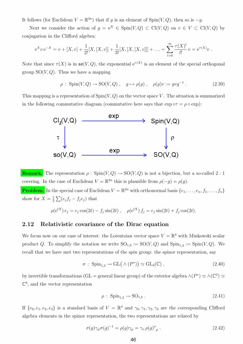
It follows (for Euclidean V = R2n) that if g is an element of Spin(V, Q), then so is −g.
Next we consider the action of g = eX ∈ Spin(V,Q) ⊂ Cl(V, Q) on v ∈ V ⊂ Cl(V,Q) by
conjugation in the Clifford algebra:
eXv e−X = v + [X, v] +1
2![X, [X, v]] +
1
3![X, [X, [X, v]]] + . . . =
∞∑
l=0
τ(X)l
l!v = eτ(X)v .
Note that since τ(X) is in so(V,Q), the exponential eτ(X) is an element of the special orthogonal
group SO(V,Q). Thus we have a mapping
ρ : Spin(V,Q) → SO(V,Q) , g 7→ ρ(g) , ρ(g)v := gvg−1 . (2.39)
This mapping is a representation of Spin(V, Q) on the vector space V . The situation is summarized
in the following commutative diagram (commutative here says that exp τ = ρ exp):
Remark. The representation ρ : Spin(V, Q) → SO(V,Q) is not a bijection, but a so-called 2 : 1
covering. In the case of Euclidean V = R2n this is plausible from ρ(−g) = ρ(g).
Problem. In the special case of Euclidean V = R2n with orthonormal basis e1, . . . , en, f1, . . . , fn
show for X = 12
∑
(ejfj − fjej) that
ρ(etX) ej = ej cos(2t) − fj sin(2t) , ρ(etX) fj = ej sin(2t) + fj cos(2t).
2.12 Relativistic covariance of the Dirac equation
We focus now on our case of interest: the Lorentzian vector space V = R4 with Minkowski scalar
product Q. To simplify the notation we write SO1,3 := SO(V,Q) and Spin1,3 := Spin(V,Q). We
recall that we have met two representations of the spin group: the spinor representation, say
σ : Spin1,3 → GL(
∧ (P ∗))
≃ GL4(C) , (2.40)
by invertible transformations (GL = general linear group) of the exterior algebra ∧(P ∗) ≃ ∧(C2) ≃
C4, and the vector representation
ρ : Spin1,3 → SO1,3 . (2.41)
If e0, e1, e2, e3 is a standard basis of V = R4 and γ0, γ1, γ2, γ3 are the corresponding Clifford
algebra elements in the spinor representation, the two representations are related by
σ(g)γµσ(g)−1 = ρ(g)γµ = γν ρ(g)νµ . (2.42)
13
The gamma matrices γµ appearing in the Dirac equation differ from the γµ by the position of the
index, which is raised or lowered by using the Minkowski metric: γµ = Q(eµ, eν)γν =: Qµνγ
ν and
γµ = Qµνγν where QµνQνλ = δµλ . We therefore have
σ(g)γµσ(g)−1 = ρ(g)γµ = Qµνρ(g)γν = QµνQλτγτρ(g)λ
ν = ρ(g−1)µνγ
ν . (2.43)
We now introduce a notion similar to that of scalar field and vector field.
Definition. A spinor field is a mapping ψ : R4 → ∧(P ∗) ≃ C
4 from space-time (viewed as a
vector space after fixing a space-time origin) into the spinor representation space. It transforms
under the spin group as
(g · ψ)(v) := σ(g)ψ(ρ(g)−1v) , (g ∈ Spin1,3 , v ∈ R4). ¤ (2.44)
The next statement has the implication that the wave function ψ of the Dirac equation is to
be viewed as a spinor field.
Proposition. If ψ is a solution of the Dirac equation with gauge potential A = Aµ dxµ, then g ·ψ
for g ∈ Spin1,3 is a solution of the same equation with transformed gauge potential
(g · A)µ(v) = ρ(g−1)νµAν(ρ(g)−1v) . (2.45)
Proof. Let ψ be a solution of
γµ
(
~
i
∂
∂xµ− eAµ
)
ψ + mc ψ = 0 . (2.46)
We multiply the equation from the left by σ(g) for g ∈ Spin1,3 and use (2.43) to obtain
ρ(g−1)µνγ
ν
(
~
i
∂
∂xµ− eAµ
)
σ(g)ψ + mc σ(g)ψ = 0 . (2.47)
It remains to transform the arguments of ψ and Aµ from v to ρ(g)−1v. For this step we use the
fact that application of the operator e−ωµ
ν xν∂µ (for ωµν ∈ R) to a function v 7→ f(v) yields
(
e−ωµ
ν xν∂µf)
(v) = f(e−ω v) , ∂µ ≡∂
∂xµ. (2.48)
We also use the formula
e−ωµ
ν xν∂µ ∂λ eωµ
ν xν∂µ = ∂λ + ωµλ ∂µ + . . . = (eω)µ
λ ∂µ .
Now we apply the operator e−ωµ
ν xν∂µ for eω ≡ ρ(g) to Eq. (2.49). This gives
ρ(g−1)µνγ
ν
(
~
iρ(g)λ
µ
∂
∂xλ− eA′
µ
)
(g · ψ) + mc (g · ψ) = 0 , (2.49)
where A′
µ(v) = Aµ(ρ(g)−1v). Since ρ(g)λµ ρ(g−1)µ
ν = ρ(gg−1)λν = δλ
ν we obtain
γµ
(
~
i
∂
∂xµ− e (g · A)µ
)
(g · ψ) + mc (g · ψ) = 0 , (2.50)
which is the desired result. ¤
14
2.13 Discrete symmetries of the Dirac equation
2.13.1 Pin group and parity transformation
Both the special orthogonal group SO(V,Q) and the spin group Spin(V, Q) are connected. (In
fact, Spin has the additional property of being simply connected, which means that every closed
path in it is contractible to a point; the latter is not the case for SO.) However the full orthogonal
group O(V, Q) has more than one connected component. In particular, the operation of space
reflection, while not contained in SO(V,Q), does belong to O(V, Q) for our case of V = R4 with
Minkowski scalar product Q. One may then ask whether there exists a group Pin(V, Q) which
is related to Spin(V, Q) in the same way that O(V, Q) is related to SO(V,Q). The answer, as it
turns out, depends on whether the quadratic form Q is definite or indefinite. In the definite (or
Euclidean) case, the answer is yes; otherwise it is only partially yes. We now briefly highlight a
few salient points in order to motivate the form of the parity operator for the Dirac equation.
The Clifford algebra comes with an automorphism α : Cl(V,Q) → Cl(V, Q) by the Z2-degree:
α(x) = x if x is even, and α(x) = −x if x is odd. The Clifford algebra also comes with an
anti-automorphism called the transpose; this is defined by 1 = 1t, vt = v for v ∈ V , and
(xy)t := ytxt .
Definition. The Clifford group Γ(V, Q) is defined as the group of invertible elements x ∈ Cl(V,Q)
with the property that twisted conjugation
Cl(V,Q) ⊃ V ∋ v 7→ xv α(x)−1
stabilizes V , i.e., maps V into itself. The group Pin(V, Q) ⊂ Γ(V,Q) is the subgroup defined as
Pin(V, Q) = x ∈ Γ(V,Q) | xtx = ±1 . (2.83)
Problem. Check that Pin(V,Q) contains Spin(V, Q). ¤
In the case of the Lorentzian vector space R1,3 (a short-hand notation for V = R
4 with
Minkowski scalar product Q) any space-like or time-like unit vector u = eµ is in Pin1,3 ≡ Pin(V,Q).
Indeed, utu = eµeµ = Q(eµ, eµ) = ±1, and
uv α(u)−1 = uv−u
Q(u, u)= v − 2u
Q(u, v)
Q(u, u)∈ V .
We see that the operation v 7→ uv α(u)−1 is a reflection at the hyperplane orthogonal to u .
Problem. For g ∈ Pin(V,Q) show that ρ(g) : V → V defined by ρ(g)v = gv α(g)−1 is an
orthogonal transformation, ρ(g) ∈ O(V, Q). ¤
Consider now the pin group element g = e1e2e3 for a Cartesian basis e1, e2, e3 of a three-
dimensional space R3 ⊂ R
1,3. The corresponding element ρ(g) ∈ O1,3 is the sequence of three
reflections at the hyperplanes orthogonal to e1, e2, and e3 . The combined effect of these reflections
37

is a space reflection, i.e., the operation of inverting each of the three Cartesian coordinates. This
operation is also called a ‘parity transformation’ in physics.
In the context of the Dirac equation one wants to work with conjugation v 7→ gvg−1 rather than
twisted conjugation gv α(g)−1. To correct for the extra minus sign inflicted by twisted conjugation,
we multiply g = e1e2e3 by a pin group element x with the property that xv x−1 = −v for all v ∈ V .
If e0 with Q(e0, ej) = 0 (j = 1, 2, 3) is a time-like unit vector, the product x = e0e1e2e3 is such an
element. Thus we arrive at xg = e0 . Since e0 is represented in the spinor representation by γ0,
the next definition is well motivated.
Definition. The operator of parity transformation acts on Dirac spinors ψ as
P : ψ(~x, t) 7→ γ0ψ(−~x, t) . (2.84)
We now look at what happens to the Dirac equation
γµ
(
~
i
∂
∂xµ− eAµ
)
ψ + mcψ = 0 (2.85)
under a parity transformation. By the chain rule of differentiation, reversal ψ(~x, t) 7→ ψ(−~x, t) of
the space arguments sends the spatial derivatives ∂/∂xj to their negatives. This sign change is
compensated by conjugation γj 7→ γ0γjγ0 = −γj (j = 1, 2, 3). We thus have the following
Fact. The Dirac equation in the absence of electromagnetic fields (Aµ = 0) is parity-invariant,
i.e., if ψ is a solution, then so is P · ψ.
Problem. Show that if ψ is a solution of the Dirac equation with gauge potential A = A0 dx0 +∑
Aj dxj, then P · ψ is a solution of the Dirac equation with transformed gauge potential
(P · A)(~x, t) = A0(−~x, t) dx0 −∑
Aj(−~x, t) dxj .
2.13.2 Anti-unitary symmetries of the Dirac equation
Going beyond parity, the Dirac equation has some discrete symmetries which do not come (not
in a physically satisfactory manner anyway) from the pin group but require complex anti-linear
operations. One of these is time reversal, T . In the standard representation (2.15) of the gamma
matrices this operation is given by
T : ψ(~x, t) 7→ γ1γ3 ψ(~x,−t) . (2.86)
Note that T 2 = −1 and
γ1γ3 =
(
iσ2 00 iσ2
)
.
Remark. By non-relativistic reduction, this formula yields the time-reversal operator (1.32) for
spin-1/2 Schrodinger particles. Note also that T normalizes Spin1,3 (T Spin1,3 T−1 = Spin1,3). ¤
To investigate the behavior of the Dirac equation under time reversal, we take its complex
conjugate and observe that γ0, γ1 and γ3 are real matrices while γ2 is imaginary (in standard
repn). We also note that t 7→ −t sends ∂t 7→ −∂t and that γ1γ3γµ(γ1γ3)−1 = ǫ γµ where ǫ = −1
38

for µ = 1, 3 and ǫ = 1 for µ = 0, 2. In this way we find that T transforms a solution ψ of the
Dirac equation (2.85) into a solution of the same equation with transformed gauge potential
(T · A)(~x, t) = −(
−A0(~x,−t) dx0 +∑
Aj(~x,−t) dxj)
.
The Dirac equation has another complex anti-linear symmetry, which is called charge conju-
gation. This operation (again, in standard representation) is defined by
C : ψ(~x, t) 7→ iγ2 ψ(~x, t) . (2.87)
The name derives from the easily verified fact that C transforms a solution ψ of the Dirac equation
into a solution C · ψ of the same equation with conjugated charge (e → −e). Notice that C2 = 1,
and CP = −PC, whereas CT = TC and PT = TP .
Consider now the combination of charge conjugation, parity, and time reversal:
CPT : ψ(~x, t) 7→ γ5 ψ(−~x,−t) , γ5 = iγ0γ1γ2γ3 . (2.88)
This combined operation is more fundamental than its individual factors in that it is defined even
in the absence of a splitting R1,3 = R ⊕ R
3 into time and space. Since each factor is a symmetry
of the Dirac equation, so is the product CPT . The precise statement is this: if ψ is a solution of
the Dirac equation with gauge field Aµ , then CPT · ψ is a solution with transformed gauge field
(CPT · A)(~x, t) = −Aµ(−~x,−t) dxµ . (2.89)
Remark. A deep result of theoretical physics is the so-called CPT theorem: any quantum field
theory which is unitary (i.e., has a Hermitian Hamiltonian for its time-evolution generator), local
(i.e., the Lagrangian contains only derivatives up to a finite order), and Lorentz-invariant, must
have CPT as a symmetry. In other words: the combined operation of running time backwards,
reflecting space, and replacing matter by anti-matter, must always be a symmetry of the funda-
mental laws of nature. Another remark is that the CPT theorem serves as important input to
the proof of the spin-statistics theorem, which says that bosons and fermions have integer and
half-integer spin, respectively.
2.13.3 Parity violation by the weak interaction
Although CPT is always a symmetry, it turns out that there do exist fundamental interactions of
nature which break one or another of the individual factors. Here we briefly indicate how parity
is broken by the weak interaction.
In the limit of zero mass (m → 0), the Dirac equation for the 4-component spinor ψ splits into
a pair of equations for two 2-component spinors ψL and ψR , which are called Weyl or half-spinors.
This works as follows. Based on γ25 = 1 for γ5 = iγ0γ1γ2γ3, one introduces projection operators
Π± = 12(1 ± γ5) . (2.90)
39

By using γµΠ± = Π∓γµ, one infers from the Dirac equation (2.85) with mass m = 0 that
0 = Π±γµ
(
~
i
∂
∂xµ− eAµ
)
ψ = γµ
(
~
i
∂
∂xµ− eAµ
)
Π∓ψ . (2.91)
Thus both ψL := Π+ψ and ψR := Π−ψ are solutions of the massless Dirac equation.
To interpret the half-spinors ψR , ψL it is best to choose the so-called Weyl representation for
the gamma matrices:
γ0 =
(
0 11 0
)
, γj =
(
0 σj
−σj 0
)
, γ5 =
(
1 00 −1
)
. (2.92)
In this representation, (the non-zero part of) ψL consists of the upper two components of ψ and
ψR consists of the lower two components. The decoupled pair of equations for ψL,R then reads
(
∂t + c∑
σj ∂j
)
ψR = 0 ,(
∂t − c∑
σj ∂j
)
ψL = 0 (2.93)
in zero electromagnetic field. In order for ψR = ei(~k· ~x−|k|ct)η to be a solution of the first equation,
the constant 2-component spinor η must be an eigenvector
~σ · ~k η = |k| η , ~σ · ~k =
(
k3 k1 − ik2
k1 + ik2 −k3
)
,
of ~σ ·~k/|k| with eigenvalue (also referred to as helicity) +1. In such an eigenvector the momentum
and spin angular momentum of the particle form a right-handed system (hence the notation ψR
and the name helicity). Similarly, in order for ψL = ei(~k· ~x−|k|ct)ξ to be a solution of the second
equation, the spinor ξ must be an eigenvector of ~σ · ~k/|k| with eigenvalue −1. In this case the
momentum and the spin angular momentum form a left-handed system. Note that Π+P = PΠ− ,
so that PψL = ψR and PψR = ψL , in agreement with the observation that space reflection
transforms a right-handed system into a left-handed one and vice versa.
Experiments on β-decay done in the mid-1950’s showed a strong right-left asymmetry of the
radioactive decay process. This is understood nowadays (from the so-called Standard Model of
elementary particle physics) as resulting from a peculiar feature of the electro-weak interaction:
left-handed particles carry electro-weak charge, but right-handed particles do not – a clear violation
of parity symmetry! More precisely, the left-handed component eL of the electron constitutes a
doublet of half-spinors
(
eL
νL
)
together with the electron neutrino, and an analogous doublet is
formed by the up and down quarks. These doublets are governed by the second equation of (2.93)
with minimal substitution ∂µ → ∂µ −Aµ where Aµ , the electro-weak gauge potential, is a 2 × 2
matrix. The off-diagonal elements of Aµ quantize as the W± boson, the diagonal elements as the
Z0 boson. The right-handed component of the electron only couples to the electromagnetic field.
40
2.14 Dirac electron in a Coulomb potential
A major application of non-relativistic quantum mechanics is the computation of the discrete
energy spectrum of the hydrogen atom using the Schrodinger equation. In this section we carry
out a similar computation based on the Dirac equation.
The first step is to choose a gauge. We take
A = Aµ dxµ = A0 dx0 = −Φ dt , (2.94)
where Φ = Ze/(4πε0r) is the Coulomb potential due to a positive nuclear charge Ze placed at
the origin of the coordinate system. As usual, r =√
x2 + y2 + z2 denotes the distance from the
origin. Adopting this gauge, the Hamiltonian for the negatively charged Dirac electron is
H =~c
i
∑
l
αl
∂
∂xl
+ βmc2 − Ze2
4πε0r. (2.95)
We are going to look for bound-state solutions of the stationary Dirac equation
Hψ = Eψ . (2.96)
Our strategy is the same as in the non-relativistic case: exploiting the spherical symmetry of the
Coulomb potential, we will reduce Hψ = Eψ to a radial differential equation. The solution of the
latter equation will then be found as a power series.
2.14.1 Using rotational symmetry
The Coulomb potential is invariant under space rotations fixing the origin (the nucleus). This
invariance will allow us to find the solution in the form of a product ansatz (separation of variables).
To begin, we recall the action of a spin group element g ∈ Spin1,3 on the spinor field ψ:
(g · ψ)(v) = σ(g)ψ(ρ(g)−1v) .
Here we want this transformation law for the special case of g ∈ Spin3 ⊂ Spin1,3, ρ ∈ SO3, and
we only need it at the infinitesimal level. Hence we put gt = etX and τ(X) = ω and differentiate
with respect to the parameter t at t = 0.
To compute the contribution from the rotation v 7→ ρ(gt)−1v of the argument of ψ , we use the
formulas ρ(gt)−1 = e−tω and f(e−tω•) = e−t
∑
ωkl xl ∂kf [see Eq. (2.80)],
e−t∑
ωkl xl∂k = ei
~t∑
ωjLj , ωkl =∑
jǫjkl ωj , Lj =
~
i
∑
klǫjkl xk ∂l =
∑
klǫjkl xk pl .
Here ǫjkl is the totally anti-symmetric tensor of R3, i.e., ǫ123 = ǫ231 = ǫ312 = 1, ǫ321 = ǫ213 = ǫ132 =
−1, and the tensor vanishes if two indices coincide.
There is a second contribution to the derivative at t = 0; this comes from multiplication
ψ 7→ σ(gt)ψ = σ(etX)ψ by the spinor representation of gt . To compute it, we use the formulas
X = τ−1(ω) =1
4
∑
klωkl γlγk =
i
2
∑
jωjΣj , Σj =
(
σj 00 σj
)
,
41

where γj represents the Cartesian basis vector ej ∈ R3 viewed as a generator of the Clifford algebra
(in the spinor representation). Putting everything together, we obtain
d
dteτ
−1(tω) · ψ∣
∣
∣
t=0=
i
~
∑
lωlJl ψ , J = L+ S , Sl =
~
2Σl . (2.97)
The interpretation of this result is clear: the total angular momentum J is the sum of orbital
angular momentum L and spin angular momentum S.
Problem. Show by direct calculation that the Dirac Hamiltonian (2.95) has vanishing commu-
tator with each of the three components of the total angular momentum J = L+ S.
It follows that [H, J2] = 0. We also have [H,P ] = 0 by the parity symmetry of the Coulomb
potential. We thus have a set of four commuting operators H, J2, J3 , P, and we will be looking
for joint eigenfunctions of this set. For this purpose, let
ϕljm :=
(
Yl ⊗ χ1/2
)
jm= aljm Yl,m−1/2 ⊗
(
10
)
+ bljm Yl,m+1/2 ⊗
(
01
)
(2.98)
be a 2-component angular momentum eigenfunction:
J2ϕljm = ~
2j(j + 1)ϕljm , J3 ϕ
ljm = ~mϕl
jm , (2.99)
L2ϕljm = ~
2l(l + 1)ϕljm , S2ϕl
jm = ~2 12(12+ 1)ϕl
jm . (2.100)
The exact details of this construction will be spelled out in the chapter on tensor invariants of the
rotation group SO3 ; here we just mention/anticipate that the coefficients aljm and bljm are so-called
Clebsch-Gordan coefficients coupling orbital angular momentum (with quantum numbers l m±12)
and spin angular momentum (with quantum numbers 12±1
2) to total angular momentum (with
quantum numbers j m):
aljm = 〈l m−12, 12
12| j m〉 , bljm = 〈l m+1
2, 12− 1
2| j m〉 . (2.101)
The main result to be used in the sequel now follows from the identity
2∑
iLi Si = (L+ S)2 − L2 − S2 = J2 − L2 − S2 .
Using it we infer that ϕljm is an eigenfunction of the operator ~σ · ~L :=
∑
σiLi :
(~σ · ~L)ϕljm = ~
(
j(j + 1)− l(l + 1)− 34
)
ϕljm = −~ (1 + κ)ϕl
jm . (2.102)
The second equation defines the parameter κ . Note that
κ =
l j = l − 12,
−l − 1 j = l + 12.
(2.103)
2.14.2 Reduction by separation of variables
We now proceed with the solution of Hψ = Eψ by making an ansatz for the 4-component spinor
ψ as a direct sum of two 2-component spinors ξ and η :
ψ =
(
ξ
η
)
. (2.104)
53

The stationary Dirac equation with Coulomb potential V (r) := −Ze2/(4πε0r) then decomposes
as a pair of coupled equations for ξ and η :
(E − mc2 − V ) ξ = c ~σ · ~p η , (2.105)
(E + mc2 − V ) η = c ~σ · ~p ξ . (2.106)
At this point we recall from (2.98) the angular momentum eigenfunction ϕljm and separate the
variables by making the product ansatz
ξ = iF (r)ϕljm , η = G(r)
~σ · ~xr
ϕljm . (2.107)
We pause briefly to subject this ansatz to a consistency check. A short calculation shows that
~σ · ~x is invariant under infinitesimal rotations:
[Jj , ~σ · ~x] =[
∑
ǫjkl xk pl + 12~σj , ~σ · ~x
]
=~
i
∑
ǫjkl xk σl + i~∑
ǫjkl σl xk = 0 .
On the other hand, space reflection ~x → −~x takes ~σ ·~x into its negative. Thus ~σ ·~x is what is called
a pseudo-scalar in physics. Now a spherical harmonic Yl mltransforms under space reflection as
Yl ml→ (−1)l Yl ml
. Therefore our ansatz has parity Pψ = (−1)lψ .
To proceed, we use the formula σjσk = δjk + i∑
ǫjkl σl to deduce the identities
(~σ · ~x)(~σ · ~p) = ~x · ~p + i~σ · (~x × ~p) = rpr + i~σ · ~L , (2.108)
(~σ · ~p)(~σ · ~x) = ~p · ~x + i~σ · (~p × ~x) = −3i~ + rpr − i~σ · ~L . (2.109)
With their help we now compute the result of applying the operator ~σ · ~p to the two-component
spinors ξ and η of (2.107):
~σ · ~p ξ =~σ · ~xr2
((~σ · ~x ) (~σ · ~p )) ξ = ~~σ · ~xr2
(
∂
∂r+
1 + κ
r
)
Fϕljm , (2.110)
~σ · ~p η =(
(~σ · ~p )(~σ · ~x ))G
rϕl
jm = i~
(
− ∂
∂r− 2
r+
1 + κ
r
)
Gϕljm . (2.111)
Finally, by making the substitutions F = r−1f and G = r−1g we bring the pair of equations
(2.105, 2.106) into the form
(E − mc2 − V )f = ~c
(
− ∂
∂r+
κ
r
)
g , (2.112)
(E + mc2 − V )g = ~c
(
+∂
∂r+
κ
r
)
f . (2.113)
We must now solve this pair of ordinary differential equations in the radial variable r.
2.14.3 Solution of radial problem
We first investigate the problem in the limit r → ∞ where the Coulomb energy V (r) ∼ 1/r and
the rotational energy κ/r become negligible and our pair of equations simplifies to
(E − mc2)f ≈ −~c∂g
∂r, (E + mc2)g ≈ ~c
∂f
∂r.
43

We easily see that this pair of asymptotic equations is solved by
f ≈ (mc2 + E)1/2 e−λr , g ≈ −(mc2− E)1/2 e−λr ,
where
λ = (~c)−1√
(mc2)2 − E2 (2.114)
is a characteristic wave number of the problem. We observe that in the non-relativistic limit
0 < mc2 − E ≪ mc2 the expression for λ reduces to
λ = ~−1
√
2m , = mc2− E ,
which is the de Broglie (imaginary) wave number for a bound state of binding energy .
These asymptotic considerations motivate the following ansatz:
f =
√
1 +E
mc2e−λr (A + B) , g =
√
1 −E
mc2e−λr(A − B) . (2.115)
with unknown functions A = A(r) and B = B(r) which behave as A → 0 and B → const for
r → ∞. To process this ansatz, it is useful to introduce the following dimensionless quantities:
ρ := 2λr , kE := ZαE
~cλ, kM := Zα
mc2
~cλ, α :=
e2
4πε0~c, (2.116)
where α ≈ 1/137 is the so-called fine structure constant. (This name is of historical origin. It is
nowadays understood that α is not a constant; being the coupling of quantum electrodynamics,
α depends logarithmically on the energy cutoff or regularization scale.)
We now insert the ansatz (2.115) into (2.112, 2.113). After some trivial (if somewhat lengthy)
algebra we arrive at the following equations for A and B :
∂A
∂ρ= A −
kE
ρA −
kM + κ
ρB ,
∂B
∂ρ=
kM − κ
ρA +
kE
ρB . (2.117)
The final step is to find the solution to these equations in the form of power series. To prepare
this step, we investigate the behavior in the limit of ρ → 0. Let
A ≃ aργ , B ≃ bργ (ρ → 0) .
By inserting this small-ρ asymptotics into (2.117) and then sending ρ → 0, we obtain the following
system of linear equations for the numbers a and b :
(γ + kE) a + (κ + kM) b = 0 ,
(κ − kM) a + (γ − kE) b = 0 .
In order for this system to have a solution other than the trivial one (a = b = 0), the determinant
of the underlying matrix must vanish:
Det
(
γ + kE κ + kM
κ − kM γ − kE
)
= γ2− k2
E − κ2 + k2
M = 0 .
44

From (2.116) we then see that k2M − k2
E = (Zα)2. Therefore the value of γ must be
γ = γ(κ) =√
κ2 − Z2α2 , (2.118)
which makes good sense as long as the nuclear charge Z is not too large.
We finally look for the solution in the form of two power series:
A =∞
∑
n=0
anργ+n , B =∞
∑
n=0
bnργ+n .
By inserting these into (2.117) and comparing coefficients we get
(n + γ + kE) an + (κ + kM) bn = an−1 ,
(κ − kM) an + (n + γ − kE) bn = 0 .
The equation for n = 0 (with a−1 = 0) has a non-trivial solution for a0 and b0 by our choice
(2.118) for γ. For n ≥ 1 we eliminate bn to obtain a recursion relation for an alone:
an =
(
(n + γ + kE) − (κ + kM)(κ − kM)
n + γ − kE
)−1
an−1 =n + γ − kE
n2 + 2nγan−1 .
A sufficient condition for a bound-state solution to emerge is that the power series terminates at
some finite order n resulting in square-integrable functions f and g. The condition for termination
is that
0 = n + γ − kE
holds for some positive integer n ≥ 1. By solving this condition for E, we arrive at the following
answer for the (discrete) energy spectrum:
En,κ =mc2
√
1 + (Zα)2
(n+γ(κ))2
. (2.119)
Problem. Show that in the non-relativistic limit c → ∞ this formula reproduces the known
energy spectrum of hydrogen as computed from the Schrodinger equation. How do n , κ relate to
the quantum numbers of the non-relativistic spectrum? ¤
45

3 Second quantization
3.1 Bosons and fermions
We are assuming that the students of this course already have some familiarity with the quantum
mechanics of a single particle and thus with quantum theory at the simplest level. As a prepara-
tion for the more advanced formalism of ‘second quantization’ introduced in this chapter, let us
summarize by means of a table what are the key elements of the correspondence between classical
mechanics and single-particle quantum mechanics.
When there is more than one particle present, new structures and phenomena related to per-
mutation symmetry appear. It turns out that the generalization to n-particle quantum mechanics
depends on whether the particles under consideration are distinguishable or indistinguishable. In
the former case the Hilbert space V of the many-particle system is simply the tensor product
V = V (1) ⊗ V (2) ⊗ · · · ⊗ V (n) (3.1)
of the Hilbert spaces V (1), . . . , V (n) for the individual particles (labeled by 1, . . . , n). Thus the wave
function for n distinguishable particles in the Schrodinger representation is a linear combination
of products of single-particle wave functions,
Ψ(x1,x2, . . . ,xn) =∑
ai1i2... in ψi1(x1)ψi2(x2) · · ·ψin(xn) , (3.2)
with complex coefficients ai1i2... in . Linear operators representing observables such as the energy
or the components of momentum, act on these wave functions in the natural way (i.e., one simply
tensors up the setting of single-particle quantum mechanics), and there isn’t a whole lot of new
material for the student to learn.
However, in the case of indistinguishable or identical particles, the many-particle Hilbert space
is spanned by wave functions which are either totally symmetric or totally anti-symmetric. Con-
sider first the latter case where we have
Ψ(x1,x2, . . . ,xn) = sign(π) Ψ(xπ(1),xπ(2), . . . ,xπ(n)) , (3.3)
50
for any permutation π ∈ Sn . [Here sign(π) = +1 if the permutation π is even and sign(π) = −1
if π is odd.] Particles with this behavior under permutations are called fermions.
Gibbs, in the context of classical statistical mechanics, observed that symmetrization (more
precisely: reduction of statistical weight by identification of n-particle configurations that are
permutations of one another) is needed in order for the entropy to be additive. The next series of
statements gives a quantum-theoretic explanation of this observation.
Fact. The wave functions for (an indefinite number of) fermions with single-particle Hilbert space
V , e.g. V = L2(R3), form an exterior algebra, ∧(V ). The wave function for a definite number n
of fermions is an element of the degree-n subspace ∧n(V ) ⊂ ∧(V ) of the exterior algebra. If Ψp
and Ψq are totally anti-symmetric wave functions describing two subsystems of p resp. q fermions
(all of which are identical), then the wave function for the total system of p + q identical fermions
is the exterior product Ψp ∧ Ψq defined by
(Ψp ∧ Ψq)(x1, . . . ,xp+q) :=1
p! q!
∑
π∈Sp+q
sign(π)Ψp(xπ(1), . . . ,xπ(p)) Ψq(xπ(p+1), . . . ,xπ(p+q)) . (3.4)
The most general n-fermion wave function ψ ∈ ∧n(V ) can be expressed as a linear combination
of exterior products of single-particle wave functions:
Ψ =∑
ai1i2... inψi1 ∧ ψi2 ∧ · · · ∧ ψin , (3.5)
with complex coefficients ai1i2... in . The vacuum state is 1 ∈ ∧0(V ) ≡ C. One also writes 1 ≡ |0〉.
Problem. Show that the exterior product is associative: (Ψp ∧ Ψq) ∧ Ψr = Ψp ∧ (Ψq ∧ Ψr) . ¤
We now turn to the alternative situation of totally symmetric wave functions:
Φ(x1,x2, . . . ,xn) = Φ(xπ(1),xπ(2), . . . ,xπ(n)) (3.6)
for any permutation π ∈ Sn . Particles with this behavior under permutations are called bosons.
Definition. If V is a K-vector space, one defines the symmetric algebra S(V ) as the associative
algebra which is generated by V ⊕ K with relations vv′ = v′v for all v, v′ ∈ V . Multiplication in
the symmetric algebra with these relations is called the symmetric product. When the symmetric
product is to be emphasized, we use the expanded notation v∨v′ = v′∨v. The symmetric algebra
is graded by the degree:
S(V ) =⊕
n≥0Sn(V ) , S0(V ) ≡ K , S1(V ) ≡ V . (3.7)
Problem. Assuming V to be of finite dimension dim V = N , show that dim Sn(V ) =
(
N + n − 1n
)
.
[Thus, unlike the exterior algebra ∧(V ), the symmetric algebra S(V ) has infinite dimension even
when V is finite-dimensional.]
Fact. The wave functions for (an indefinite number of) bosons with single-particle Hilbert space
V form the symmetric algebra S(V ). Any wave function for a definite number n of bosons is
an element of the degree-n subspace Sn(V ) ⊂ S(V ) of the symmetric algebra. If Φp and Φq are
51

totally symmetric wave functions describing two subsystems of p resp. q bosons (all of which are
identical), then the wave function for the total system of p + q bosons is the symmetric product
(Φp ∨ Φq)(x1, . . . ,xp+q) =1
p! q!
∑
π∈Sp+q
Φp(xπ(1), . . . ,xπ(p)) Φq(xπ(p+1), . . . ,xπ(p+q)) . (3.8)
The most general n-boson wave function Φ ∈ Sn(V ) can be expressed as a linear combination of
symmetric products of single-particle wave functions:
Φ =∑
ai1i2... in φi1 ∨ φi2 ∨ · · · ∨ φin . (3.9)
The boson vacuum state is |0〉 ≡ 1 ∈ S0(V ) ≡ C. ¤
To do many-particle quantum mechanics, one must understand how to turn physical observ-
ables into operators on the many-particle Hilbert spaces ∧(V ) for fermions and S(V ) for bosons.
The present chapter will introduce a good algebraic formalism by which to handle the situation,
namely ’second quantization’. Second quantization for bosons is particularly suitable as a for-
malism to quantize the abelian gauge theory of electromagnetism. Another application will be
to the Dirac equation: using second quantization for fermions one reinterprets Dirac’s original
single-electron theory as a quantum field theory which remains stable and physically meaningful
even in the presence of coupling to the quantized electromagnetic field.
3.2 Weyl algebra and Clifford algebra
We now introduce a boson-type analog of the Clifford algebra.
Definition. Let U be a symplectic vector space over the number field K , i.e., U carries a non-
degenerate skew-symmetric (or alternating) K-bilinear form
A : U × U → K , A(u, u′) = −A(u′, u) . (3.10)
The Weyl algebra of U is defined to be the associative algebra, W(U,A), generated by U ⊕K with
relations
uu′ − u′u = A(u, u′) . (3.11)
Remark. Without changing the content of the theory, we could enhance the similarity with the
definition of the Clifford algebra in Section 2.7 by putting 2A instead of A on the right-hand side.
Nonetheless, in the present context we prefer to use the normalization convention (3.11).
Example 1. Consider the symplectic plane (or phase plane) U = R2 with basis vectors e, f and
symplectic form
A(e, e) = A(f, f) = 0 , A(e, f) = −A(f, e) = −1 . (3.12)
The Weyl algebra W(R2, A) then is the algebra of polynomial expressions in e and f with real
coefficients and the relation fe − ef = 1 being understood. A concrete realization of this algebra
is by a polynomials in a coordinate generator x ≡ e and its derivative d/dx ≡ f .
52

Example 2. We give a second example, which is closer to the setting pursued below. Let q and
p be the position and momentum operators of a one-dimensional quantum system. Let K = C ,
U = spanCp , q, and take A to be the Heisenberg commutator:
A(q, q) = A(p, p) = 0 , A(q, p) = −A(p, q) = i~ . (3.13)
Then the Weyl algebra W(U,A) is the algebra of polynomials in the operators q and p . A specific
example of such a polynomial is the Hamiltonian H = p2/2m + mω2q2/2 of the one-dimensional
harmonic oscillator. Introducing the dimensionless operators
a :=1√2
(
q
ℓ+ i
ℓp
~
)
, a† :=1√2
(
q
ℓ− i
ℓp
~
)
, (3.14)
where ℓ =√
~/(mω) is the oscillator length, one can also view the Weyl algebra W(U,A) as the
algebra of polynomials in the operators a and a† with commutation relations
a a† − a†a = 1 . (3.15)
The oscillator Hamiltonian is known to take the form H = ~ω(a†a + 12). ¤
We now start introducing the formalism of second quantization for bosons. For this we realize
the notion of Weyl algebra as follows. Let V be the single-boson Hilbert space and let V ∗ be its
dual. (We shall refrain from using the isomorphism cV : V → V ∗, v 7→ 〈v, ·〉V by the Hermitian
scalar product of V for the moment.) We take the direct sum U = V ⊕ V ∗ to be equipped with
the canonical alternating form A : U × U → C ,
A(v + ϕ, v′ + ϕ′) = ϕ(v′) − ϕ′(v) . (3.16)
With these definitions, the Weyl algebra W(V ⊕ V ∗, A) is the algebraic structure underlying (the
formalism of second quantization for) many-boson quantum systems.
Definition. In physics the following notational conventions are standard. One fixes some basis
e1, e2, . . . of the single-boson Hilbert space V with dual basis f1, f2, . . . of V ∗, and one writes
fi ≡ ai and ei ≡ a+i . Using the duality pairing fi(ej) = δij , one then gets the Weyl algebra
relations (3.11) in the form
[ai , a+j ] = δij , [ai , aj] = [a+
i , a+j ] = 0 (i, j = 1, 2, . . .) . (3.17)
These are called the canonical commutation relations (CCR).
Remark. Later, ai and a+i will be acting as linear operators in the so-called bosonic Fock space
S(V ) with its canonical Hermitian scalar product. In that setting, assuming that e1, e2, . . . is
an orthonormal basis, the operator a+i ≡ a†
i will turn out to be the Hermitian adjoint of ai .
Example. By the canonical commutation relations one has
a+i aj a+
k al = a+i a+
k aj al + δjk a+i al . ¤ (3.18)
53
In view of the close similarity between the Weyl algebra and the Clifford algebra, one may
ask whether a development parallel to that of Sections 2.10 and 2.11 exists on the bosonic side.
The answer is: yes, to a large extent. Indeed, the analog of SO(V, Q) is the symplectic Lie group
Sp(U,A), the analog of so(V,Q) is the symplectic Lie algebra sp(U,A), and the analog of Cl2(V,Q)
is the subspace
W2(U,A) := X ∈ W(U,A) | X =∑
i(uivi + viui) ; ui , vi ∈ U
of symmetrized degree-2 elements of the Weyl algebra. It is still true that W2(U,A) is a Lie
algebra which is isomorphic to sp(U,A) by letting X ∈ W2(U,A) act on u ∈ U ⊂ W(U,A) by
the commutator, and that by exponentiating this commutator action one recovers the symplectic
Lie group. There is, however, one difference: it is not possible to exponentiate W2(U,A) inside
the Weyl algebra to produce an analog of the spin group. The reason is that, by a theorem due
to Stone and von Neumann, any non-trivial realization of the Weyl algebra with relations (3.11)
must be on an infinite-dimensional representation space where the elements X ∈ W2(U,A) act as
unbounded operators. For example, the Hamiltonian H of the harmonic oscillator is an element
H ∈ W2(U,A) for our Example 2 above. The exponential e−tH exists for Re t > 0 but does not
for Re t < 0 . Nonetheless, in a suitable real framework there does exist a bosonic analog of the
spin group; it is called the metaplectic group. (For example, the quantum time evolution of the
harmonic oscillator is a one-parameter subgroup of the metaplectic group.)
This concludes our introduction of the Weyl algebra and the canonical commutation relations
for bosons. We now turn to the fermionic side: the Clifford algebra. Here we will be brief, as we
have already given a thorough discussion of the Clifford algebra in Chapter 2.
Definition. The formalism of second quantization for fermions is based on the following. Starting
from the single-fermion Hilbert space V , we take the direct sum U = V ⊕V ∗ and we equip U with
the symmetric bilinear form B : U × U → C defined by
B(v + ϕ, v′ + ϕ′) = ϕ(v′) + ϕ′(v) . (3.19)
The Clifford algebra Cl(U,B) then is the associative algebra generated by U ⊕ C with relations
uu′ + u′u = B(u, u′) . (3.20)
In physics it is customary to use the following notational conventions. Fixing any basis e1, e2, . . .
of the single-fermion Hilbert space V with dual basis f1, f2, . . . of V ∗, one writes fi ≡ ci and
ei ≡ c+
i . By the duality pairing fi(ej) = δij , one then gets the Clifford algebra relations (3.20) in
the form
ci , c+
j = δij , ci , cj = c+
i , c+
j = 0 (i, j = 1, 2, . . .) , (3.21)
where u, u′ := uu′ + u′u denotes the anti-commutator. We recall from Section 2.8 that the
relations (3.21) are referred to as the canonical anti-commutation relations (CAR).
54

3.3 Representation on Fock space
In Section 2.8 we learned that the abstract Clifford algebra Cl(V ⊕V ∗, B) has a concrete realization
by linear operators on the spinor representation space ∧(V ). [Actually, we constructed the spinor
representation for V = P ∗. Note that V and V ∗ are on the same footing in this context, and
exactly the same construction would go through for the choice ∧(P ∗) = ∧(V ∗) of representation
space.] We will now explain that, in a very similar way, the abstractly defined Weyl algebra
W(V ⊕ V ∗, A) has a realization by linear operators on the so-called bosonic Fock space S(V ).
Note that A(v, v′) = A(ϕ, ϕ′) = 0 vanishes for any v, v′ ∈ V and ϕ, ϕ′ ∈ V ∗. One expresses this
fact by saying that V and V ∗ are Lagrangian subspaces of the complex symplectic vector space
U = V ⊕ V ∗. It follows from the Weyl algebra relations (3.11) that vv′ = v′v and ϕϕ′ = ϕ′ϕ.
These are the defining relations of the respective symmetric algebras, namely S(V ) and S(V ∗).
We thus see that both S(V ) and S(V ∗) are contained as subalgebras in W(V ⊕ V ∗, A).
We can now get a representation of W(V ⊕ V ∗, A) by letting it act on S(V ), or S(V ∗), or any
other subalgebra generated by a Lagrangian subspace. We focus on S(V ) for concreteness. Thus
our goal now is to define an action of W(V ⊕ V ∗, A) on S(V ),
W(V ⊕ V ∗, A) × S(V ) → S(V ) , (x, ξ) 7→ x · ξ . (3.22)
Since W(V ⊕ V ∗, A) is generated by V ⊕ V ∗ ⊕ C , it suffices to specify the Weyl multiplication
(3.22) for vectors v ∈ V and co-vectors ϕ ∈ V ∗. (The multiplication by scalars k ∈ C is of course
the obvious one given by the structure of a complex vector space.)
Multiplication by vectors v ∈ V is simply the symmetric product computed inside the sym-
metric algebra:
v · ξ := µ(v) ξ := v ∨ ξ ≡ v ξ . (3.23)
The notation µ(v) is used in order to distinguish the algebra element v ∈ V ⊂ W(V ⊕ V ∗, A)
from its concrete realization as a linear operator µ(v) on S(V ). Note that this multiplication
µ(v) : Sl(V ) → Sl+1(V ) increases the degree (in physics language: the number of bosons) by one.
Now consider ϕ ∈ V ∗. Such elements act by a degree-lowering operation δ(ϕ) :
δ(ϕ) : Sl(V ) → Sl−1(V ) , ξ 7→ ϕ · ξ ≡ δ(ϕ) ξ , (3.24)
which is called a derivation of S(V ), as it has the algebraic properties of a derivative. We define
it recursively. For the two lowest degrees l = 0, 1 we set
l = 0 : δ(ϕ) 1 := 0 , (3.25)
l = 1 : δ(ϕ) v := ϕ(v) . (3.26)
The action on higher-degree elements ξ ∨ η ∈ S(V ) is then defined by the product rule (or Leibniz
rule) known from differential calculus:
δ(ϕ) (ξ ∨ η) := δ(ϕ)ξ ∨ η + ξ ∨ δ(ϕ)η . (3.27)
55

Problem. Show that the operations of symmetric multiplication µ(v) : Sl(V ) → Sl+1(V ) and
derivation δ(ϕ) : Sl(V ) → Sl−1(V ) satisfy the canonical commutation relations (CCR):
µ(v)µ(v′) − µ(v′)µ(v) = 0 , δ(ϕ)δ(ϕ′) − δ(ϕ′)δ(ϕ) = 0 ,
δ(ϕ)µ(v) − µ(v)δ(ϕ) = A(ϕ, v) IdS(V ) , (3.28)
for all v, v′ ∈ V and ϕ, ϕ′ ∈ V ∗. ¤
Using the canonical commutation relations, an easy calculation
(v + ϕ) · ((v′ + ϕ′) · ξ) − (v′ + ϕ′) · ((v + ϕ) · ξ) − A(v + ϕ, v′ + ϕ′) · ξ
=(
µ(v) + δ(ϕ))(
µ(v′) + δ(ϕ′))
ξ −(
µ(v′) + δ(ϕ′))(
µ(v) + δ(v))
ξ − A(v + ϕ, v′ + ϕ′)ξ
= δ(ϕ)µ(v′)ξ − µ(v′)δ(ϕ)ξ − A(ϕ, v′)ξ − δ(ϕ′)µ(v)ξ + µ(v)δ(ϕ′)ξ + A(ϕ′, v)ξ = 0 ,
shows that the relations (3.11) are satisfied for all v + ϕ = u and v′ + ϕ′ = u′. Thus we have
indeed constructed a representation of W(V ⊕ V ∗, A).
Definition. For a complex vector space V let the direct sum V ⊕ V ∗ be equipped with the
canonical alternating form A(v + ϕ, v′ + ϕ′) = ϕ(v′) − ϕ′(v). The oscillator representation of the
Weyl algebra W(V ⊕ V ∗, A) is defined by the action
(v + ϕ + k) · ξ = µ(v)ξ + δ(ϕ)ξ + kξ (v ∈ V, ϕ ∈ V ∗, k ∈ C) (3.29)
on the symmetric algebra S(V ). ¤
Let us now give the translation into the language and notation of physics. We recall that the
symmetric algebra S(V ) is referred to as the bosonic Fock space (of the single-particle Hilbert
space V ) in this context. The neutral element 1 ∈ S0(V ) = C is called the vacuum state and is
denoted by 1 ≡ |0〉. (To avoid confusion, we emphasize that |0〉 is not the zero vector!) We also
recall that fixing an orthonormal basis e1, e2, . . . of V together with the dual basis f1, f2, . . . of
V ∗, one writes a+i ≡ ei and ai ≡ fi and refers to these as particle creation and particle annihilation
operators, respectively. No change of notation is made when these algebraically defined objects act
as linear operators on the bosonic Fock space. Thus ai ≡ δ(fi) and a+i ≡ µ(ei). The definitions
of multiplication a+j = µ(ei) : Sl(V ) → Sl+1(V ) and derivation aj = δ(fj) : Sl(V ) → Sl−1(V )
translate to
a+j ·
(
a+i1a+
i2· · · a+
il|0〉
)
:= a+j a+
i1a+
i2· · · a+
il|0〉 , (3.30)
aj ·(
a+i1a+
i2· · · a+
il|0〉
)
:= δji1a+i2a+
i3· · · a+
il|0〉
+ δji2a+i1a+
i3· · · a+
il|0〉 + . . . + δjila
+i1a+
i2· · · a+
il−1|0〉 . (3.31)
56

The action (3.35) of the particle annihilation operator aj = δ(aj) is also defined by saying that
the canonical commutation relations (3.17) hold and
aj|0〉 = 0 . (3.32)
This concludes, for the moment, our development of the bosonic variant of second quantization,
and we turn to a summary and adaptation of the material of Chapter 2 for the fermionic side.
Definition (Review). For a complex vector space V let the direct sum V ⊕ V ∗ be equipped
with the canonical symmetric form B(v + ϕ, v′ + ϕ′) = ϕ(v′) + ϕ′(v). The spinor representation
of the Clifford algebra Cl(V ⊕ V ∗, B) is defined by the action
(v + ϕ + k) · ξ = ε(v)ξ + ι(ϕ)ξ + kξ (v ∈ V, ϕ ∈ V ∗, k ∈ C) (3.33)
on the exterior algebra ∧(V ). In physics one calls ∧(V ) the fermionic Fock space. The vacuum
is denoted by |0〉 ≡ 1 ∈ ∧0(V ). Introducing an orthonormal basis as usual, the actions of the
particle creation operator ε(ej) ≡ c+j and particle annihilation operator ι(fj) ≡ cj are given by
c+j ·
(
c+i1c+i2· · · c+
il|0〉
)
:= c+j c+
i1c+i2· · · c+
il|0〉 , (3.34)
cj ·(
c+i1c+i2· · · c+
il|0〉
)
:= δji1c+i2c+i3· · · c+
il|0〉
− δji2c+i1c+i3· · · c+
il|0〉 + . . . + (−1)l−1 δjilc
+i1c+i2· · · c+
il−1|0〉 . (3.35)
The particle annihilation operators cj = ι(fj) annihilate the vacuum: cj|0〉 = 0 . ¤
We finish the section with a tabular summary:
57

3.4 Fock space scalar product
We are in the process of developing a quantum-theoretic formalism for many bosons and/or
fermions. What we have learned so far is how the single-particle Hilbert space V gets promoted
to a Fock space S(V ) or ∧(V ) for many particles. In order to turn Fock space into the Hilbert
space of many-body quantum theory, we still need to introduce a Hermitian scalar product on it.
Given that the single-particle Hilbert space V already carries a Hermitian scalar product 〈·, ·〉V ,
there is a natural way of doing this, as follows.
For bosons and fermions alike, the Fock space scalar product is diagonal in the degree or
particle number n . For bosons one defines the scalar product 〈·, ·〉Sn(V ) : Sn(V )× Sn(V ) → C by
⟨
v1 ∨ v2 ∨ · · · ∨ vn , v′1 ∨ v′2 ∨ · · · ∨ v′n
⟩
Sn(V )=
∑
π∈Sn
〈v1, v′π(1)〉V 〈v2, v′π(2)〉V · · · 〈vn, v′π(n)〉V . (3.36)
Notice that in the special case of vn = v∨v∨· · ·∨v (n factors) one has 〈vn, v′n〉Sn(V ) = n!〈v, v′〉nV .
Using physics notation, this means that
(a+1 )n1
√n1!
(a+2 )n2
√n2!
· · · (a+l )
nl
√nl!
· · · |0〉 (3.37)
for nl ∈ N ∪ 0 (l = 1, 2, . . .) is an orthonormal basis of S(V ), provided that the standard
convention a+i = µ(ei) is in force and e1, e2, . . . is an orthonormal basis of V .
The Hermitian scalar product 〈·, ·〉∧n(V ) : ∧n(V )× ∧n(V ) → C for fermions is defined by
⟨
v1 ∧ · · · ∧ vn , v′1 ∧ · · · ∧ v′n
⟩
∧n(V )=
∑
π∈Sn
sign(π) 〈v1, v′π(1)〉V · · · 〈vn, v′π(n)〉V
= Det
〈v1, v′1〉V · · · 〈v1, v′n〉V...
. . ....
〈vn, v′1〉V · · · 〈vn, v′n〉V
. (3.38)
It can be shown that this has all the properties required of a Hermitian scalar product; in partic-
ular, 〈v1 ∧ · · · ∧ vn , v1 ∧ · · · ∧ vn〉∧n(V ) is non-negative and vanishes only if v1 ∧ · · · ∧ vn is the zero
vector. The latter happens if and only if the set of vectors v1 . . . , vn is linearly dependent. This
feature is called the Pauli exclusion principle.
Assuming again the standard physics convention c+i = ε(ei) for an orthonormal basis e1, e2, . . .of V , one finds that the set of Fock space vectors
(c+1 )n1(c+2 )
n2 · · · (c+l )nl · · · |0〉 (3.39)
for nl ∈ 0, 1 (l = 1, 2, . . .) constitute an orthonormal basis of ∧(V ).
Problem. We recall that for a complex vector space with Hermitian scalar product, one has a
canonically defined operation of taking the Hermitian adjoint (denoted by †). Show that (c+j )† = cj
(fermions) and (a+j )† = aj (bosons).
65

There exists another perspective on the Hermitian scalar product in Fock space, as follows.
We recall that the Hermitian scalar product 〈·, ·〉V on single-particle Hilbert space V determines
a one-to-one correspondence
cV : V → V ∗, v 7→ 〈v, ·〉V ,
called the Dirac ket-bra bijection and written |v〉 7→ 〈v| in Dirac’s notation. Consider now the
case of fermions for definiteness (for bosons it works the same way). The map cV induces on the
fermionic Fock space ∧(V ) a mapping
c∧(V ) : ∧(V ) → ∧(V )∗ ≃ ∧(V ∗) , v1 ∧ · · · ∧ vn 7→ cV (vn) ∧ · · · ∧ cV (v1) . (3.40)
(Such a mapping is called an anti-homomorphism of exterior algebras, as the order of factors is
reversed.) In physics notation (with standard conventions) this reads
c∧(V ) : c+i1c+i2· · · c+
in|0〉 7→ 〈0|cin · · · ci2ci1 .
The r.h.s. 〈0|cin · · · ci1 is a linear function on the fermionic Fock space ∧(V ) and as such an element
of ∧(V )∗ in the natural way: to evaluate this linear function on a vector c+j1· · · c+
jn|0〉 in Fock space
we apply the product cin · · · ci1 and then take the vacuum component:
c∧(V )
(c+i1c+i2· · · c+
in|0〉
) (c+j1
c+j2· · · cjn
|0〉)
= 〈0|cin · · · ci2ci1c+j1
c+j2· · · cjn
|0〉 .
By using the canonical anti-commutation relations to compute the right-hand side we obtain
c∧(V )
(c+i1c+i2· · · c+
in|0〉
) (c+j1
c+j2· · · cjn
|0〉)
=∑
π∈Sn
sign(π)n∏
l=1
δil, jπ(l),
in agreement with the definition (3.38). Thus we may regard the Fock space Hermitian scalar
product (3.38) as a manifestation of the natural mapping (3.40).
3.5 Second quantization of one- and two-body operators
Let now L ∈ End(V ) be a linear operator on the single-particle Hilbert space V . Such an operator
is called a one-body operator in the present context. We fix some basis e1, e2, . . . (not necessarily
orthonormal) and denote by f1, f2, . . . the dual basis of V ∗.
Definition. The process of second quantization for fermions or bosons sends the one-body oper-
ator L ∈ End(V ) to the operator L on Fock space ∧(V ) resp. S(V ) which is defined by
L 7→ L =
∑i
ε(Lei)ι(fi) (fermions),∑i
µ(Lei)δ(fi) (bosons).(3.41)
Fact. The second-quantized operator L extends the one-body operator L ∈ End(V ) as a derivation
of the algebra under consideration, i.e., as a derivation of the exterior algebra ∧(V ) for the case
of fermions and of the symmetric algebra S(V ) for the case of bosons.
59

Proof. Consider the case of fermions and let v ∈ V ⊂ ∧(V ) be any single-particle state. Appli-
cation of L yields
Lv =∑
iε(Lei)ι(fi)v =
∑ifi(v) ε(Lei)1 =
∑ifi(v) Lei = Lv .
Thus L coincides with L on the single-particle subspace V = ∧1(V ). Now consider an n-particle
state ξ = v1∧v2∧· · ·∧vn which is a product of n single-particle states. By applying the annihilation
operator ι(fi) you get
ι(fi)ξ = ι(fi)v1 ∧ v2 ∧ · · · vn − v1 ∧ ι(fi)v2 ∧ · · · ∧ vn + . . . + (−1)n−1v1 ∧ v2 ∧ · · · ∧ ι(fi)vn .
Subsequent exterior multiplication by ε(Lei) and summation over i gives
Lξ = Lv1 ∧ v2 ∧ · · · vn + v1 ∧ Lv2 ∧ · · · ∧ vn + . . . + v1 ∧ v2 ∧ · · · ∧ Lvn .
This formula precisely expresses the fact that L is a derivation of the exterior algebra ∧(V ).
For bosons the argument is the same albeit for some sign changes.
Problem. Show that second quantization of one-body operators is a Lie algebra homomorphism,
i.e., [L,M ] = [L, M ]. ¤
Adopting the standard physics conventions, we now choose our basis of V to be an orthonormal
basis |i〉i=1,2,... (Dirac notation), and we write ε(ei) ≡ c+i , ι(fi) ≡ ci , µ(ei) ≡ a+
i , δ(fi) ≡ ai .
The second quantization rule (3.41) for fermions or bosons then takes the form
L 7→ L =
∑i,j
〈i|L|j〉 c+i cj (fermions),
∑i,j
〈i|L|j〉 a+i aj (bosons).
(3.42)
Example. Consider Schrodinger particles confined to a cube C with side length L and periodic
boundary conditions. The single-particle Hilbert space is V = L2(C) and an orthonormal basis of
V is given by the plane waves
ψk(x) = L−3/2eik·x
for the discrete set of wave vectors
k = (k1, k2, k3) ∈ (2πZ/L)3 =: Λ .
Orthonormality here means that∫
C
ψk(x)ψk′(x) d3x = δkk′ .
The one-body operator T := −~2∇2/2m of the Schrodinger kinetic energy has matrix elements
〈k|T |k′〉 =~2k2
2mδkk′ , k2 = k2
1 + k22 + k2
3 ,
and the second-quantized kinetic energy T is
T =∑
k∈Λ
εk c+kck
, εk =~2k2
2m.
60

The operator c+kck
is called the occupation number operator (for the single-particle state with
momentum p = ~k). It has two eigenvalues: 0 (empty state) and 1 (occupied state).
Remark. The homomorphism property [L, M ] = [L, M ] does not single out (3.42) but also holds
for other schemes of second quantization. For example, it holds for
L 7→ L =
∑i,j
〈i|L|j〉 cic+j (fermions),
−∑i,j
〈i|L|j〉 aia+j (bosons).
(3.43)
The reason is that ci ↔ c+i is an automorphism of the Clifford algebra, and ai → a+
i , a+i → −ai
is an automorphism of the Weyl algebra. The fermionic version of this ‘hole quantization’ scheme
will become relevant in the reinterpretation of the Dirac equation as a quantum field theory. ¤
We now turn briefly to the scheme of second quantization for two-body operators. By definition,
a two-body operator is a linear operator
L : V ⊗ V → V ⊗ V (3.44)
defined on the tensor product of two single-particle Hilbert spaces. (While these may be different
when the two particles are distinguishable, we here continue to focus on the case of identical
particles.) If we work in the Schrodinger representation and ϕi(x) (i = 1, 2, . . .) is a basis of
single-particle wave functions, then the two-body matrix elements of L are expressed as
〈ij|L|kl〉 :=
∫
R3
∫
R3
ϕi(x) ϕj(x′) (L(ϕk ⊗ ϕl)) (x,x′) d3x d3x′ . (3.45)
Example. The Coulomb interaction energy UC between two particles with charge e is the two-
body operator given by
(UC(ϕk ⊗ ϕl)) (x,x′) =e2
4πε0 |x − x′|ϕk(x)ϕl(x
′) . (3.46)
It has two-body matrix elements
〈ij|UC|kl〉 =e2
4πε0
∫
R3
∫
R3
ϕi(x) ϕj(x′) ϕk(x)ϕl(x′)
|x − x′|d3x d3x′ . ¤ (3.47)
Second quantization sends a two-body operator L to an operator L on Fock space. Given
a single-particle basis and the corresponding two-body matrix elements 〈ij|L|kl〉 this works as
follows:
L 7→ L =
12
∑ijkl
〈ij|L|kl〉 c+i c+
j cl ck (fermions),
12
∑ijkl
〈ij|L|kl〉 a+i a+
j al ak (bosons).(3.48)
The factors of 12
and reversal of the order of annihilation operators are needed in order for the
second-quantized operator L to agree with the defining operator L on the two-particle subspace
∧2(V ) or S2(V ). Note that by the commutation relations for fermions/bosons one may (anti)-
symmetrize the two-body matrix elements in the expression for L :
L =
14
∑ijkl
(〈ij|L|kl〉 − 〈ij|L|lk〉) c+i c+
j cl ck (fermions),
14
∑ijkl
(〈ij|L|kl〉 + 〈ij|L|lk〉) a+i a+
j al ak (bosons).(3.49)
The second summand 〈ij|L|lk〉 is called the exchange matrix element.
61

3.6 Second quantization of Dirac’s theory
3.6.1 Motivation: problems with the Dirac equation
The Dirac equation was originally conceived as a relativistic wave equation for a single charged
particle, by the analogy with the Schrodinger equation. In the non-relativistic limit with weak
electromagnetic fields, the single-particle interpretation of the Dirac equation works just fine.
However, serious problems of interpretation arise in the presence of strong electromagnetic
fields. One problematic situation has already been discussed in the problem class; we here review
it. Addressing the Dirac equation Hψ = Eψ for stationary states in the case of an electric scalar
potential with a step:
V =
0 z < 0 ,V0 z > 0 ,
let us look for a plane-wave solution ψ with incoming wave boundary conditions ψin ∼ eikz. Thus
we employ an ansatz as a sum
ψ = a+eikz
E + mc2
0~kc0
Θ(−z) + a− e−ikz
E + mc2
0−~kc
0
Θ(−z) + b eik′z
E − V0 + mc2
0~k′c0
Θ(z)
of reflected and transmitted waves. [We use the spinor representation in its standard form with
gamma matrices given by (2.10).] The stationary Dirac equation Hψ = Eψ is solved by this
ansatz for z < 0 if k = (~c)−1√
E2 − (mc2)2 and for z > 0 if
k′ = ±(~c)−1√
(E − V0)2 − (mc2)2 .
The ratios a−/a+ and b/a+ are determined by requiring continuity of the solution ψ at z = 0 .
The situation of interest now occurs when V0 > E + mc2. In that case we have a transmitted
wave ∼ eik′z with real wave number k′ > 0 and the stationary conserved probability current
j = ψ†αzψ = 2(|a+|2 − |a−|
2)(E + mc2)~kc = 2|b|2(E − V0 + mc2)~k′c < 0
is negative. This phenomenon implies, in particular, that the reflection probability |r|2 = |a−/a+|2
exceeds unity! Certainly, there exists no satisfactory interpretation of such a result within the
confines of unitary single-particle quantum mechanics.
62

Mathematical analysis of the situation reveals that the paradoxical behavior has its reason in
the existence of stationary solutions with negative energy E − V0 < −mc2.
Furthermore, the Dirac Hamiltonian, as it stands, does not have a ground state: it is bounded
neither from below nor from above. When the interaction with the quantized electromagnetic field
is switched on, the absence of a lower bound for the Dirac Hamiltonian poses the catastrophic
threat that an infinite amount of electromagnetic energy might be released by Dirac particles
making a never ending series of transitions to states with lower and lower energy.
These problems force us to abandon the single-particle interpretation of the Dirac equation.
In fact, the correct physical interpretation of the result |a−/a+|2 > 1 above is in terms of particle
production (namely, the creation of electron-positron pairs at the potential step). The paradox
is then resolved by reinterpreting the current vector field ~j = ψ†~αψ – which had originally been
intended to be a conserved probability current – as a conserved electric current.
3.6.2 Stable second quantization
As we have tried to indicate, there are serious problems with the original form of Dirac’s theory
due to the fact that the Dirac Hamiltonian, being unbounded from below, does not have a ground
state. Therefore, we now look for a reformulation of Dirac’s theory such that the Hamiltonian
does have a ground state. In the present section we make preparations for such a reformulation
by taking the formalism of second quantization to its most general form.
Let H ∈ End(V ) be any Hermitian Hamiltonian on a single-particle Hilbert space V ; our
interest, of course, is in Hamiltonians H which resemble the Dirac Hamiltonian in that they have
positive as well as negative spectrum neither of which is bounded. We will describe a procedure of
second quantization H 7→ H which sends H to a non-negative operator H ≥ 0 on the Fock space
∧(P ∗) for a suitably chosen subspace P ∗ ⊂ V ⊕ V ∗. Our procedure consists of two steps.
In the first step we convert H ∈ End(V ) into an element HC ∈ Cl(V ⊕ V ∗, B) of the Clifford
algebra of the direct sum V ⊕V ∗ with canonical symmetric form B(v +ϕ, v′ +ϕ′) = ϕ(v′)+ϕ′(v).
To describe this step, let e1, e2, . . . be any basis of V and f1, f2, . . . be the dual basis of V ∗.
Expanding Hei =∑
j ejHji with respect to that basis, we define
HC :=∑
ij
Hji ej fi (3.50)
as a quadratic element of the Clifford algebra Cl(V ⊕ V ∗, B). The Clifford algebra element HC is
seen to be invariantly defined, i.e., does not depend on the choice of basis. Note that our object
HC is still formal and abtract: we have not yet specified the space which HC will be acting on.
Our second step is to choose an exterior algebra ∧(P ∗) for Cl(V ⊕ V ∗, B) to act on. The
choice will be engineered in precisely such a manner that the second-quantized Hamiltonian H
representing HC comes out to be non-negative.
Assuming that H has no zero eigenvalue, let Π± be the uniquely defined orthogonal projection
63

operators for the positive and negative eigenspaces V+ = Π+V and V− = Π− of H. In formulas:
H = H+ + H− , H± = Π±HΠ± , H+ > 0 > H− . (3.51)
We now recall from Section 2.8 that a spinor representation of the Clifford algebra Cl(W,B)
is constructed by choosing a polarization
W = P ⊕ P ∗ (3.52)
by Lagrangian subspaces P, P ∗. In the present setting, one such polarization W = V ⊕ V ∗ is
given a priori. The key point, however, is that we should replace it by another one to obtain a
well-behaved second-quantized Hamiltonian H. In fact, the good choice of polarization for our
purposes is
P = V ∗+ ⊕ V− , P ∗ = V+ ⊕ V ∗
− . (3.53)
Thus we reverse the roles of vector space and dual space (and hence the definitions of creation
and annihilation operator) when switching from the H-positive eigenspace V+ to the H-negative
eigenspace V− .
We also recall from Section 2.8 that, given a polarization W = P ⊕ P ∗, the Clifford algebra
generators w ∈ W ⊂ Cl(W,B) act by the spinor representation on ξ ∈ ∧(P ∗) as a mixture
w · ξ := ι(wP ) ξ + ε(wP ∗) ξ (3.54)
of exterior multiplication ε(wP ∗) (or particle creation) for the P ∗-component and contraction ι(wP )
(or particle annihilation) for the P -component of w.
Definition. Let H = H++H− be the decomposition of a Hermitian Hamiltonian H ∈ End(V ) into
its positive and negative parts, neither of which is bounded. If V = V+ ⊕ V− is the corresponding
decomposition into H-positive and H-negative subspaces, let ei, ek be any two bases of V+ ,
V− , and fj, fl the dual bases of V ∗+ , V ∗
− , respectively. By the positive (or stable) second
quantization of H we then mean the operator H on ∧(V+ ⊕ V ∗−) defined by
H :=∑
ij
(H+)ij ε(ei) ι(fj) −∑
kl
(H−)kl ε(fl) ι(ek) . (3.55)
Thus the elements of P ∗ = V+⊕V ∗− act as particle creation operators (ε) and those of P = V ∗
+⊕V−
as particle annihilation operators (ι).
Remark. Note that by CAR the expression (3.55) can be rewritten as
H =∑
ij
(H+)ij ε(ei) ι(fj) +∑
kl
(H−)kl
(ι(ek) ε(fl) − δkl
). (3.56)
Written in this form, stable second quantization clearly implements the standard scheme (3.54)
but for the subtraction of an (infinite) constant∑
kl(H−)kl δkl = Tr H− . This subtraction in
combination with the adjustment of the order of operators ι(ek) ε(fl)− δkl = −ε(fl) ι(ek) is called
normal ordering.
64
Fact. The stable second quantization H defined by (3.55) is positive.
Proof. The operator H is a derivation of the exterior algebra ∧(P ∗). By this token it is positive
on ∧(P ∗) if it is positive on the degree-one subspace P∗ ⊂ ∧(P ∗). Now H acts on V+ ⊂ P
∗ as
H+ > 0 and on V∗
−as −H
t
−> 0 . Therefore H is positive on P
∗ = V+ ⊕ V∗
−as desired.
3.6.3 The idea of hole theory
In the next subsection, the mathematical idea of stable second quantization will be used to fix the
problems with the Dirac equation. Before doing so, let us give a simplified discussion.
The main physical idea is to redefine what is meant by the vacuum. To consider a very simple
example, let |0〉 be the (naive) vacuum for a one-dimensional single-particle Hilbert space V ≃ C ,
and denote by c+ (c) the particle creation (resp. annihilation) operator as usual. The Hamiltonian
in this one-dimensional case is just a real number H = h ∈ R . If h is positive, the standard
scheme H 7→ H = h c+c ≥ 0 of second quantization is fine. On the other hand, for h < 0 the
scheme must be changed if H is to be non-negative. There exist two equivalent ways of going
about this. One is to exchange the roles of c+ ↔ c and replace c
+c by cc
+ − 1 = −c+c (that’s
what we did in Section 3.6.2). Equivalently, we may leave the operators the same and, instead,
adjust the definition of the vacuum:
|vac〉 := c+|0〉 .
Indeed, by the Pauli exclusion principle c+c+ = 0 we now have c
+|vac〉 = 0 . Thus c+ acts on the
new vacuum as an annihilation operator. At the same time we have c|vac〉 = |0〉 6= 0, so c now
plays the role of a creation operator. And by subtracting a constant from the Hamiltonian
H := hc+c − h
in order to make the energy of the new vacuum vanish (which amounts to a redefinition of the
location of zero on the energy axis), we obtain
H(c|vac〉) = −h (c|vac〉)
and thus an excited state c|vac〉 with positive energy eigenvalue −h > 0 .
Going from this example to the setting of the Dirac equation, the idea of Dirac’s hole theory is
to define the true vacuum to be the state in which each negative-energy stationary solution of the
Dirac equation is occupied by one electron (and hence Pauli blocked), while all positive-energy
solutions are unoccupied. The fully occupied negative-energy sector is often referred to as the
‘Dirac sea’. Although the true vacuum |vac〉 has infinite energy and infinite charge relative to
the naive vacuum |0〉, one still commands the freedom of shifting the observables of energy and
charge so that they vanish for |vac〉. The elementary excitations of the true vacuum then are
particles c+
+|vac〉 in positive-energy states and hole excitations c−|vac〉 of the Dirac sea. The latter
have positive energy as well as positive charge (as the negative energy and negative charge of one
Dirac-sea electron are missing); they are interpreted as the states of a new elementary particle
predicted by this reinterpretation of the Dirac equation: the positron.
65

.
3.6.4 Mode expansion of the Dirac field
We now implement the scheme of stable second quantization for the Hamiltonian of the Dirac
equation. As we recall, the first step of the scheme is to convert the Dirac Hamiltonian H =
βmc2 +∑
αlplc into a quadratic Clifford algebra element HC . Using the basis offered by spinors
ψ(x) in the position representation, this is achieved by
HC :=
∫
d3x
4∑
τ=1
(Hψ)†τ(x) ψτ (x) , (3.57)
where ψ henceforth is called the Dirac field. Its components obey the canonical anti-commutation
relations
ψτ (x), ψτ ′(x′) = 0 , ψ†τ(x), ψ†
τ ′(x′) = 0 , ψτ (x), ψ†
τ ′(x′) = δττ ′ δ(x − x′) . (3.58)
The second step is to construct a good Fock space ∧(P ∗) for HC to act on. For this we need
the decomposition of the single-particle Hilbert space V = L2(R3) ⊗ C4 into its H-positive and
H-negative subspaces V+ and V− . By the translation invariance of H the projection operators
(Π±ϕ)τ (x) =
∫
d3x′∑
τ ′
(Π±)ττ ′(x − x′) ϕτ ′(x′) (3.59)
on these subspaces have Fourier expansions
(Π±)ττ ′(x − x′) =
∫
d3k
(2π)3eik·(x−x
′)(Π±)ττ ′(k) , (3.60)
where Π±(k) are the matrices of the projection operators at fixed wave vector k . The latter are
found by diagonalizing the Dirac Hamiltonian
H(k) =
(
mc2~c~σ · ~k
~c~σ · ~k −mc2
)
(3.61)
in momentum representation. The 4 × 4 matrix H(k) squares to (~ω(k))2 IdC4 where
~ω(k) =√
(mc2)2 + (~ck)2 , k = |k| . (3.62)
Its eigenvalues are ±~ω(k), each with multiplicity two. Let us(k) and vs(k) denote a corresponding
set of eigenspinors:
H(k)us(k) = +~ω(k) us(k) , H(k)vs(k) = −~ω(k) vs(k) , (3.63)
with normalization u†s(k)us′(k) = v†
s(k)vs′(k) = δss′ . Because of the two-fold spin degeneracy
there remains some freedom in the definition of the quantum number s. One possible choice is
66

to take us(k) and vs(k) to be eigenvectors of the helicity operator ~Σ · ~k/k – cf. Eq. (2.97) – with
eigenvalue s = ±1.
From the eigenspinors us(k) and vs(k) one constructs the projection matrices
Π+(k) =∑
s=±1
us(k)⊗ u†s(k) , Π−(k) =
∑
s=±1
vs(k)⊗ v†s(k) , (3.64)
and from these in turn the momentum space representation of Hamiltonian:
H(k) = ~ω(k)(Π+(k)− Π−(k)
). (3.65)
We are now in a position to specify the fermionic Fock space ∧(P ∗) for the Dirac field ψ . Let
P := Π+V ⊕ (Π−V )∗. Introducing
c+, s(k) :=
∫d3x e−ik·x u†
s(k)ψ(x) ∈ Π+V ⊂ P , (3.66)
we take c+, s(k) to be the annihilation operator for an electron with momentum ~k and helicity
s. On the other hand we define
c†−,−s(−k) :=
∫d3x e−ik·x v†
s(k)ψ(x) ∈ Π−V ⊂ P ∗ (3.67)
to be the creation operator for a positron with momentum −~k and helicity −s. These operators
satisfy CAR with the non-vanishing anti-commutators being
c†+, s(k), c+, s′(k
′) = δss′
∫d3x ei(k−k
′)·x = δss′(2π)3δ(k− k′) , (3.68)
and similar for c− . In this way we get a decomposition ψ = Π+ψ +Π−ψ,
(Π+ψ)(x) =
∫d3k
(2π)3eik·x
∑
s
us(k) c+, s(k) , (3.69)
(Π−ψ)(x) =
∫d3k
(2π)3e−ik·x
∑
s
v−s(−k) c†−, s(k) , (3.70)
which is called a mode expansion of the Dirac field.
By construction, the second-quantized Hamiltonian (after normal ordering) is positive:
H =
∫d3k
(2π)3~ω(k)
∑
s
(c†+, s
(k) c+, s(k) + c†−, s(k) c−, s(k)
)≥ 0 . (3.71)
The operator of total momentum carried by the Dirac field is expressed as
p =
∫d3k
(2π)3~k
∑
s
(c†+, s
(k) c+, s(k) + c†−, s(k) c−, s(k)
). (3.72)
This concludes our discussion of the procedure of second quantization for the free Dirac field.
It remains to explain what happens in the presence of an electromagnetic field. This will be done
in a later section.
74

3.7 Quantization of the electromagnetic field
Quantization of the electromagnetic field proceeds by the formalism of second quantization for
bosons. Let us review that formalism and bring it into a form well suited to our present goals.
3.7.1 Review and consolidation
The general starting point of second quantization for bosons is a real vector space W — the phase
space of generalized positions and momenta — with symplectic form α : W ×W → R . (We here
renege on our earlier practice of using the symbol A , as A in the present context stands for the
electromagnetic gauge field.) More generally, in geometric quantization one would start from a
symplectic manifold W , but since the Maxwell theory of electromagnetism is a linear theory, it
suffices for our purposes to assume the setting of a vector space. We recall from Section 3.2 that
the symplectic vector space (W,α) determines a Weyl algebra W(W,α).
To quantize the theory and construct a quantum mechanical Hilbert space, it does not suffice
just to have a symplectic structure α on W . One also needs a complex structure J , i.e., a linear
mapping
J ∈ End(W ) , J2 = −IdW . (3.73)
It is a requirement that J induces a Euclidean scalar product
g : W × W → R , (w, w′) 7→ g(w,w′) = g(w′, w) , g(w,w) ≥ 0 , (3.74)
(or, in the more general case of a symplectic manifold W : a Riemannian metric and thus a Kahler
structure) by the formula
∀w,w′ ∈ W : g(w,w′) = α(w, Jw′) . (3.75)
Problem. Deduce from (3.75) that g(Jw, Jw′) = g(w, w′) and α(Jw, Jw′) = α(w,w′). ¤
The choice of g isn’t a big issue as long as dim W < ∞ , but it does become essential in the
case of an infinite-dimensional phase space W where different choices of g lead to inequivalent
quantizations. In our treatment of the quantized electromagnetic field, the Euclidean structure g
will be provided by the electromagnetic energy, which is a positive function.
Example. Consider the symplectic plane
W = spanReq , ep ≃ R
2
with generators eq and ep . The symplectic form (dual to the Poisson bracket) is
α(ep , eq) = −α(eq , ep) = 1 , α(eq , eq) = α(ep , ep) = 0 .
You should think of the dual basis functions q , p as the variables of position and momentum. In
the language of differential forms, one writes α = dp ∧ dq .
68

We now equip W with a Euclidean structure g (i.e., a Euclidean scalar product g) by picking
some harmonic oscillator Hamiltonian H = p2/2m + mω2q2/2 and setting
g(eq , eq) :=2
ωH(eq) = mω , g(ep , ep) :=
2
ωH(ep) = (mω)−1 ,
and g(eq , ep) = g(ep , eq) = 0 . The complex structure J ∈ End(W ) is then given by
Jeq = −mω ep , Jep = (mω)−1eq ,
or equivalently, in terms of the canonical transpose J t ∈ End(W ∗) of J ,
J tq = (mω)−1p , J tp = −mωq .
Note that J is the operator of time evolution by one quarter of the oscillator period. ¤
We continue with the general development. The complex structure J determines a polarization
W ⊗ C = V ⊕ V (3.76)
by complex subspaces V and V which are acted upon by J as J |V = −i and J |V = +i (hence the
name ‘complex structure’). The complex vector space V is called the holomorphic part of W ⊗C ,
while V is the anti-holomorphic part. Note the characterization
V = w + iJw | w ∈ W , V = w − iJw | w ∈ W . (3.77)
Thus V is isomorphic to W as a real vector space by W∼→ V , w 7→ w + iJw , and an analogous
statement holds for V .
Let the complex linear extension of α to W ⊗ C still be denoted by the same symbol α .
Problem. Show that the pairing
α : V ⊗ V → C , v ⊗ v 7→ α(v, v) , (3.78)
between V and V is non-degenerate. Show also that the subspaces V and V are Lagrangian, i.e.,
α(v, v′) = α(v, v′) = 0 for any two vectors v, v′ ∈ V and v, v′ ∈ V . ¤
By the pairing between the complex vector spaces V and V we may identify V with the dual
vector space V ∗ of V . Planck’s constant ~ has not appeared in the discussion so far, but it now
does. The point is that there is some freedom in making the identification V ≃ V ∗. Concretely
put, one has the freedom of inserting a multiplicative constant (−i/~) in the isomorphism
I : V → V ∗ , v 7→ − i
~α(v, ·) . (3.79)
By this choice of quantization constant we henceforth identify V ∋ v ≡ I(v) ∈ V ∗.
Problem. In the context of our example (the symplectic plane), show that
I (eq − iJeq) =i
~(p + iJ tp) .
69

The interpretation of this result is that p = −i~ eq =~
i
∂∂q
.
Definition/Fact. The holomorphic Lagrangian subspace V ⊂ W ⊗C carries a Hermitian scalar
product h : V × V → C by
h(v, v′) ≡ h(w − iJw,w′ − iJw′) :=i
~α(w + iJw,w′ − iJw′) . (3.80)
Remark. The same can be done on V . Concerning h on V , notice that
Reh(v, v′) =2
~g(w,w′) , Imh(v, v′) =
2
~α(w,w′) . (3.81)
It follows that h has the required properties h(v, v′) = h(v′, v) and h(v, v) ≥ 0 .
The definition (3.80) turns V ≃ V ∗ into a complex Hilbert space. The bosonic Fock space then
is the symmetric algebra S(V ∗) equipped with the Hermitian scalar product which is induced by
that of V ∗ ≃ V ; see Section 3.4 for the details. The Weyl algebra of the symplectic vector space
(W,α) acts on S(V ∗) by
w · ξ := δ(wV ) ξ + µ(wV ∗) ξ , w ∈ W, ξ ∈ S(V ∗) . (3.82)
As before in Section 3.4, the symbol δ(wV ) stands for the operator of derivation by the V -compo-
nent of w, and µ(wV ∗) means multiplication by the V ∗-component of w.
Problem. Returning to our previous example, namely the symplectic plane W = spanReq , epwith mass parameter m and oscillator frequency ω, show that
V ≡ V ∗ = C · a+ , a+ =1√2
(q
ℓ− i
ℓp
~
).
Using the isomorphism V ∗ ≃ V and the Hermitian scalar product h prove that a+ is a unit vector:
h(a+, a+) = 1. Finally, use the Fock space scalar product induced by h to compute the Hermitian
adjoint of a+ and show that
(a+)† = a =1√2
(q
ℓ+ i
ℓp
~
).
3.7.2 More preparations
Beginning with a quick reminder of some relevant material from classical electrodynamics, we now
apply the general formalism of (second) quantization to the electromagnetic field.
The electromagnetic gauge field is a one-form A = −Φ dt +∑
Aj dxj . From it one obtains
the electromagnetic field strength, a two-form F = B + E ∧ dt , by taking the exterior derivative
F = dA . In components one has
Ej = − ∂Φ
∂xj
− ∂Aj
∂t, Bij =
∂Aj
∂xi
− ∂Ai
∂xj
. (3.83)
The components of the excitations D =∑
i<j Dij dxi ∧ dxj and H =∑
Hj dxj are given by
Dij = ε0∑
kǫijk Ek , Bij = µ0
∑kǫijk Hk , (3.84)
77

where ε0 and µ0 are called the dielectric constant and magnetic permeability of the vacuum,
respectively. A short-hand form of these so-called constitutive laws is
D = ε0 ⋆ E , B = µ0 ⋆ H , (3.85)
or ⋆D = ε0 E, ⋆B = µ0 H. The fields D and B are subject to the constraints dB = 0 and dD = ρ ,
where ρ = ρ d3x is the three-form of the electric charge density. The dynamical equations of
motion are Faraday’s law B = −dE of induction and the Ampere-Maxwell law D = +dH.
Notation. Using the traditional vector notation, one expresses the two-form components Dij =
−Dj i as Dij =∑
ǫijk Dk and combines the three components into a vector D := (D1, D2, D3). The
same convention is used for the magnetic field strength B. With this convention, the constitutive
laws read D = ε0E and B = µ0H . The constraints are div B = 0 and div D = ρ , and the
equations of motion are B = −rotE and D = rotH. ¤
We will be using the Hamiltonian formalism (as opposed to the Feynman path integral formal-
ism). The standard textbook approach is to work with the gauge field A and choose the temporal
gauge Φ = 0 . In this case the magnetic vector potential A =∑
Aj dxj plays the role of the
position variable q of Hamiltonian mechanics, and the electric field strength E = −A acquires the
meaning of (minus the) velocity q . The electric excitation D corresponds to the momentum p .
However, the general framework developed in Section 3.7.1 is rather flexible: it allows us to
circumvent the introduction of the gauge field (and the ensuing need for gauge fixing) and instead
work with the physically observable field strengths and excitations directly. This is what we shall
do in the sequel. The equations will be set up in a way that likens the electron excitation D to
the position variable and the magnetic field strength B to the momentum variable.
The first step of quantization is to identify the phase space of the electromagnetic field. This
will be the space W of all solutions to Maxwell’s equations. W is an affine space, as the difference
of two solutions in the presence of sources (i.e., electric charges) is a solution of the vacuum
Maxwell equations, which form a linear system. In the current section, we will address only the
somewhat simplified problem of quantizing the electromagnetic field in the absence of charged
matter, in which case W is a vector space. (Indeed, the sum of two vacuum solutions is another
vacuum solution).
3.7.3 Symplectic structure
To quantize the theory following the general scheme of Section 3.7.1, we need a symplectic and a
complex structure on the space W of vacuum solutions. We begin with the symplectic structure.
Because every solution is determined by a set of initial data, say B|t=0 and D|t=0 , one can
compute the symplectic structure α as an integral over the Euclidean space R3 at the initial time
t = 0 . For mathematical simplicity, let us assume that the electromagnetic field is confined to
a bounded region U ⊂ R3 with Dirichlet boundary conditions D|∂U = 0 = B|∂U at the surface
∂U . (For a precise treatment, one might also take the domain U to be connected and simply
71

connected.) The following definition of the symplectic structure is modeled after the expression
α = dp ∧ dq (or α = p ∧ q = −q ∧ p in the case of a linear system) of Section 3.7.1.
Notation. If B is the two-form of the magnetic field strength (or, for that matter, any closed
two-form) then by d−1B we mean any one-form A such that dA = B. Equivalently, using the
language of vector calculus, if B is the magnetic field (or, for that matter, any divergenceless
vector field) then by rot−1B we mean any magnetic vector potential A such that rotA = B.
Fact. Let D and B be closed (i.e. dD = dB = 0). Then the integral
∫
U
D ∧ d−1B =
∫
U
D · rot−1B d3x
is independent of the choice of one-form d−1B provided that D vanishes on ∂U . Indeed, if A
and A′ satisfy B = dA = dA′ then by the Poincare lemma there exists a function f such that
A− A′ = df and
∫
U
D ∧ A−∫
U
D ∧ A′ =
∫
U
D ∧ df =
∫
∂U
fD −∫
U
fdD = 0 .
In vector notation, the same computation for the case of a gauge transformation A = A′ + gradf
looks as follows:
∫
U
D · (A−A′) d3x =
∫
U
D · gradf d3x =
∫
∂U
f D · d2n−∫
U
f divD d3x = 0 .
Remark 1. From magnetostatics one knows that if the equation B = rotA is solved for A in the
Coulomb gauge divA = 0 (or, in the language of differential forms, B = dA with d ⋆ A = 0) then
one has
A(x) =
∫
U
rotB(x′)
4π|x− x′| d3x′.
Thus with this choice of gauge we obtain the expression
∫
U
D · rot−1B d3x =
∫
U
D(x) · rotB(x′)
4π|x− x′| d3x′d3x .
Remark 2. Under certain special circumstances the integral∫D ∧ d−1B has a beautiful ge-
ometric (actually, topological) interpretation. Suppose that both D and B are localized inside
tubular neighborhoods of two curves, say γ and γ respectively. Suppose further that these tubular
neighborhoods do not intersect each other. Then it is possible to show that our integral coincides
with the Gauss linking number G(γ, γ′) of the two curves, multiplied by the product of electric
(ΦD =∫D) and magnetic (ΦB =
∫B) fluxes circulating in the tubular neighborhoods of the two
curves: ∫
U
D ∧ d−1B = ΦD ΦB G(γ, γ′).
79

Fact. The symplectic structure α on the space W of vacuum solutions, as represented by the
initial data D ≡ D|t=0 and B ≡ B|t=0 , is expressed by
α((D,B), (D ′, B ′)
)=
∫
U
(D ′ ∧ d−1B −D ∧ d−1B ′)
=
∫
U
(D′ · rot−1B−D · rot−1B′) d3x. (3.86)
In particular, α is non-degenerate on W .
How do we know that α as defined in (3.86) is the proper symplectic form to use? The answer
is that α in combination with the Hamiltonian function (the electromagnetic energy) gives the
correct Hamiltonian equations of motion, B = −dE and D = dH.
To conclude this subsection, we make a dimension check. Recall that D and B have the
physical dimensions
[D] = charge , [B] = [A] = energy/current . (3.87)
Equivalently, the components have the physical dimensions
[Dij] = charge/area , [Bij] = energy/(current×area) , [Aj] = energy/(current×length) .
It follows that∫D ∧ d−1B has the physical dimension of
charge× energy
current= energy× time = action . (3.88)
The process of quantization makes α dimensionless by measuring it in units of Planck’s constant.
3.7.4 Complex structure
The complex structure on the space W of vacuum solutions is determined by considering the total
electromagnetic energy,
H =1
2
∫
U
(D ∧ E +B ∧H) =1
2ε0
∫
U
|D|2 d3x+1
2µ0
∫
U
|B|2 d3x ≥ 0 , (3.89)
which is the classical Hamiltonian function of the theory. The details are as follows.
The equations of motion B = −dE and D = dH for the electromagnetic field on the bounded
domain U have a fundamental system of periodic solutions, the so-called normal modes. Explicit
expressions for these can be given if U has a simple regular shape such as a cube or a ball;
otherwise one is only assured of their existence and needs a numerical algorithm (typically involving
discretization on a grid) to compute them. To find the normal modes, one looks for solutions of
the wave equation (1
c2∂2
∂t2−∆
)ft = 0 , ft
∣∣∂U
= 0 , (3.90)
of stationary type. (∆ is the Laplacian, and c = 1/√ε0µ0 is the speed of light.) The ansatz
ft = f e−iωt leads to the Helmholtz equation
(ω2/c2 +∆
)f = 0 , ft
∣∣∂U
= 0 . (3.91)
80

For the type of domain U which we envisage, solutions of this equation exist only for a discrete
set of characteristic frequencies ωλ .
Problem. Show that if D is a closed electric-type two-form solution of the Helmholtz equation
with frequency ω, then d ⋆ D = ε0 dE is a closed magnetic-type two-form solution with the same
frequency. In vector notation, the statement is that by taking the curl of a divergenceless vector
solution D one gets a divergenceless (axial) vector solution rotD .
In the following, let (Dλ, Bλ) denote the electric and magnetic initial data of any two-form
solution of the Helmholtz equation with frequency ωλ . Such a pair (Dλ, Bλ) is called a normal
mode. The normal modes for a fixed characteristic frequency ωλ form a vector space Wλ . If there
are no degeneracies in the spectrum of the Laplacian (that’s the generic situation for a domain U
of arbitrary shape which we henceforth assume) Wλ is two-dimensional. The symplectic form α
on W restricts to a non-degenerate symplectic form αλ on Wλ . In fact, one has
α((0, d ⋆ Dλ), (Dλ, 0)
)=
∫
U
Dλ ∧ ⋆Dλ =
∫
U
|Dλ|2 d3x 6= 0 .
The complex structure J acts diagonally w.r.t. the decompositionW = ⊕Wλ by normal modes.
To compute its action on any one of the subspaces Wλ ⊂ W , one computes the time evolution of
the initial data (Dλ, Bλ) ⊂ Wλ for one quarter of the period Tλ = 2π/ωλ .
We are now in a position to get specific.
Definition/Fact. The complex structure acts on Wλ as
J(Dλ, Bλ
)=
(d ⋆ Bλ
ωλ µ0
, −d ⋆ Dλ
ωλ ε0
), J
(Dλ,Bλ
)=
(rotBλ
ωλ µ0
, −rotDλ
ωλ ε0
). (3.92)
Problem. Verify from the equations of motion D = d ⋆B/µ0 and B = −d ⋆D/ε0 that J(Dλ, Bλ)
as specified is indeed the quarter-period time evolution of (Dλ, Bλ). Show also that J2 = −Id .
(Hint: for the latter, the key step is to show that (d⋆)2 agrees with the Laplacian −∆ on closed
two-forms. In vector notation this means that rot rot = −∆ on divergenceless vector fields.)
3.7.5 Fock space: multi-photon states
With the symplectic and complex structures in hand, we now take a look at the induced Euclidean
scalar product g. By implementing the general prescription of (3.75) we obtain
g((Dλ, Bλ), (Dλ, Bλ)
)= α
((Dλ, Bλ), J(Dλ, Bλ)
)
=1
ωλ ε0
∫
U
Dλ ∧ ⋆Dλ +1
ωλ µ0
∫
U
Bλ ∧ ⋆Bλ =2
ωλ
H(Dλ, Bλ) ≥ 0 , (3.93)
for any normal mode (Dλ, Bλ) ∈ Wλ . Thus the Euclidean length squared of a normal mode is
equal to (twice) the electromagnetic energy of that mode divided by its characteristic frequency.
Problems. (i) Show that the normal mode subspaces Wλ are orthogonal to one another with re-
spect to the Euclidean structure g. (ii) Verify the validity of the invariance properties g(Jw, Jw′) =
g(w,w′) and α(Jw, Jw′) = α(w,w′) in the present context.
81
Next we use the complex structure J to polarize the complexified phase space W ⊗C = V ⊕ V
by two complex Lagrangian subspaces V = ⊕Vλ and V = ⊕Vλ . This can be done separately for
each normal mode λ . Hence, for every λ let Vλ be the complex one-dimensional space
Vλ = C ·((Dλ, Bλ)− iJ(Dλ, Bλ)
)(3.94)
spanned by any (non-vanishing) normal mode (Dλ, Bλ) ⊂ Wλ . We fix a special generator
eλ :=1√2
((Dλ
0 , Bλ0 )− iJ(Dλ
0 , Bλ0 ))∈ Vλ (3.95)
by normalizing to the oscillator ground state energy:
H(Dλ0 , B
λ0 ) =
1
2~ωλ . (3.96)
By recalling the Hermitian scalar product h which is given by Reh = 2g/~ and Imh = −2α/~
on the holomorphic subspace V (cf. Section 3.7.1), we see that the normalized mode eλ is a unit
vector of h. The corresponding generator of the anti-holomorphic part Vλ ⊂ Wλ ⊗ C is
eλ :=1√2
((Dλ
0 , Bλ0 ) + iJ(Dλ
0 , Bλ0 )). (3.97)
We now form the orthogonal sums V := ⊕λVλ and V := ⊕λVλ and thus have a polarization
W ⊗ C = V ⊕ V (3.98)
by Lagrangian holomorphic and anti-holomorphic subspaces. The Hilbert space of the quantized
electromagnetic field is the symmetric algebra S(V ) completed to an L2-space by the Fock space
Hermitian scalar product due to h. The state vectors in the degree-n subspace Sn(V ) are called
n-photon states. As usual, the multiplication operators a+λ := µ(eλ) act on Fock space S(V ) as
photon creation operators a+λ : Sn(V ) → Sn+1(V ), the derivations aλ := δ(eλ) : Sn(V ) → Sn−1(V )
are photon annihilation operators. The Fock space has a vacuum 1 ∈ C = S0(V ) which is denoted
by |0〉 in Dirac notation. The commutation relations are the canonical ones (CCR):
[aλ , a+
λ′ ] = δλλ′ , [a+λ , a+λ′ ] = 0 , [aλ , aλ′ ] = 0 . (3.99)
We can now write down the quantized electromagnetic field in the form of a normal mode
expansion:
D =∑
λ
(eDλ a+λ + eDλ aλ
), B =
∑λ
(eBλ a+λ + eBλ aλ
), (3.100)
where the electric and magnetic components of eλ , eλ are
eDλ =1√2
(Dλ
0 + id ⋆ Bλ
0
ωλ µ0
), eDλ =
1√2
(Dλ
0 − id ⋆ Bλ
0
ωλ µ0
),
eBλ =1√2
(Bλ
0 − id ⋆ Dλ
0
ωλ ε0
), eBλ =
1√2
(Bλ
0 + id ⋆ Dλ
0
ωλ ε0
).
By inserting the expansion (3.100) of the quantum fields D and B into the expression (3.89) for
the electromagnetic energy, we obtain the quantum Hamiltonian of the electromagnetic field as
H ?= 1
2
∑λ~ωλ
(a+λ aλ + aλ a
+
λ
). (3.101)
82

We can now write down the quantized electromagnetic field in the form of a normal mode
expansion:
D =∑
λ
(eD
λ a+λ + eD
λ aλ
), B =
∑λ
(eB
λ a+λ + eB
λ aλ
), (3.100)
where the electric and magnetic components of eλ , eλ are
eDλ =
1√2
(Dλ
0 + id ⋆ Bλ
0
ωλ µ0
), eD
λ =1√2
(Dλ
0 − id ⋆ Bλ
0
ωλ µ0
),
eBλ =
1√2
(Bλ
0 − id ⋆ Dλ
0
ωλ ε0
), eB
λ =1√2
(Bλ
0 + id ⋆ Dλ
0
ωλ ε0
).
By inserting the expansion (3.100) of the quantum fields D and B into the expression (3.89) for
the electromagnetic energy, we obtain the quantum Hamiltonian of the electromagnetic field as
H ?= 1
2
∑λ
~ωλ
(a+
λ aλ + aλ a+λ
). (3.101)
3.7.6 Casimir energy
We are now confronted with the same situation that already existed in the case of the Dirac field:
an infinite constant must be subtracted from the Hamiltonian H in order to make it well-defined
on the Fock space S(V ). Indeed, applying (3.101) to the Fock vacuum |0〉 , which is annihilated
by each of the aλ , we get an infinite ground state energy
12
∑λ
~ωλ = ∞ . (3.102)
The infinite constant to be subtracted is universal in the sense that it does not depend on the
cavity U under consideration: it is the infinite ground state energy of the electromagnetic field
for the basic situation that U covers all of space and the boundary conditions are pushed to the
edge of the universe. This universal vacuum energy differs by a finite amount EC from the infinite
ground state energy (3.102). Thus the correct formula for the quantum Hamiltonian H = HU is
HU =∑
λ~ωλ a+
λ aλ + EC(U) . (3.103)
EC is called the Casimir energy. We mention in passing that over the last decade, advanced
techniques have been developed to compute EC(U) accurately for a cavity U of general shape.
A simple dimensional estimate of EC can be had for the case of a cavity of high symmetry, say
a ball BL of radius L. For this purpose note that the characteristic frequencies ωλ secretly carry
a factor of c (speed of light). Therefore EC must be proportional to ~c, which has the physical
dimension of energy×length. Since the ball radius L is the only length scale in the problem, there
exists only one energy that can be formed:
EC(BL) ∼ ~c
L. (3.104)
Thus EC(BL) = K~c/L, where K is a constant which turns out to be negative.
The Casimir energy tends to lead to an attractive force between surfaces. This so-called
Casimir effect is predicted to be a challenge for future developments of nano-technology, as the
attractive Casimir force makes nano-particles clump together, whereas the nano-engineer would
like them to be freely movable.
75

3.7.7 Mode expansion for the torus geometry
Let us now consider a geometry which is simple enough to make it possible for the mode expansion
to be given in explicit form: we choose for U a 3-torus T3, i.e., a cubic domain
T3 = [0, L1] × [0, L2] × [0, L3]
with periodic boundary conditions in each direction. Aside from being a mathematical idealization
that does not correspond to the real world, this choice has a certain drawback: on T3 there exist
harmonic two-forms, i.e., solutions of the Laplace equation ∆D = 0 = ∆B. Such solutions require
a separate treatment beyond that of Section 3.7.5. For brevity, we will ignore this issue here.
Our main task in this section is to construct closed two-form solutions of the Helmholtz equa-
tion and thus the unit normal modes eλ and eλ . It is a standard fact that the Helmholtz equation
(∆ + k2)f = 0 for functions f has a complete orthonormal system of solutions by plane waves
fk := (L1L2L3)−1/2ei(k1 x1+k2 x2+k3 x3) , ki ∈ 2πZ/Li .
To obtain the desired solutions for D and B, we proceed as follows. For every wave vector
(actually, wave form) k = (k1, k2, k3) we choose two so-called polarization unit vectors ǫs(k)
(s = 1, 2) with two properties: (i) they form an orthonormal basis of the plane perpendicular to
the wave vector k (that’s the null plane of the wave form k), and (ii) the 3-bein (ǫ1(k), ǫ2(k), k)
is a right-handed system. (Let us mention in passing that such a choice does not exist in a
globally smooth manner in the k-continuum. Indeed, on topological grounds any smooth vector
field k 7→ ǫs(k) tangent to the two-sphere must have at least two zeroes. This obstacle is of no
concern to us here, as our set of wave vectors is discrete due the periodic boundary conditions.)
For every (k, s) we then introduce a basic, spatially constant two-form
βk, s := ι(ǫs(k)) (dx1 ∧ dx2 ∧ dx3)
= ǫs(k)1 dx2 ∧ dx3 + ǫs(k)2 dx3 ∧ dx1 + ǫs(k)3 dx1 ∧ dx2 . (3.105)
Problem. Show that the two-form bk, s := fk βk, s is closed (dbk, s = 0) and solves the Helmholtz
equation (∆ + ω2/c2) bk, s = 0 with characteristic frequency ω = |k| c . ¤
Using the information gained from the Problem, one shows that the unit normal modes are
eBk, s :=
√12µ0~ c|k| bk, s , eB
k, s = eBk, s , eD
k, s = id ⋆ eB
k, s
|k|cµ0
, eDk, s = eD
k, s . (3.106)
The mode expansion (3.100) then takes the form
D =∑
k, s
(eD
k, s a+k, s + eD
k, s ak, s
), B =
∑k, s
(eB
k, s a+k, s + eB
k, s ak, s
). (3.107)
Problems. (i) Show that the quantized fields have the correct physical dimensions [D] = charge
and [B] = energy/current. (ii) What special choice(s) did we make in (3.106) ?
76
Problems. (i) Show that the quantized fields have the correct physical dimensions [D] = charge
and [B] = energy/current. (ii) What special choice(s) did we make in (3.106) ?
3.8 Matter-field interaction
We have discussed in some detail the quantization of the free Dirac field and the free electro-
magnetic field. Let us add here a few words about the full interacting theory (called quantum
electrodynamics, or QED) of the Dirac field coupled to the electromagnetic field.
For the purpose of writing a formula for the interaction, it is necessary to introduce a magnetic
vector potential A = rot−1B, or A = d−1B. To eliminate the redundant gauge degrees of freedom
one fixes the gauge, say by choosing the Coulomb gauge
div A = 0 or d ⋆ A = 0 . (3.108)
By direct transcription from (3.107) one then has the mode expansion
A =∑
k, s
(eA
k, s a+k, s + eA
k, s ak, s
),
eAk, s =
õ0~ c
2|k|
fk
i
3∑
j=1
(−1)2−sǫ3−s(k)j dxj , eAk, s = eA
k, s . (3.109)
It is easy to check that d ⋆ eAk,s = 0, and deA
k,s = eBk,s so dA = B.
In the presence of electric charges it is no longer possible to choose the gauge Φ = 0 . Instead,
one takes Φ to be the (instantaneous) Coulomb potential determined by Poisson’s equation
∆Φ(x) = −ρ(x)/ε0 = −eψ†(x)ψ(x)/ε0 . (3.110)
The quantized Hamiltonian of the coupled theory then is
H =
∫ψ†
(∑
l
αl
(~
i
∂
∂xl
− eAl
)+ βmc2
)ψ d3x +
1
2
∫ (D ∧ E + B ∧ H
), (3.111)
where the quantum field D of the electric excitation is subject to the Gauss-law constraint dD = ρ .
The matter-field interaction here is in the term∑
Al jl coupling the magnetic vector potential to
the electric current density. By inserting the respective mode expansions, one obtains contributions
to the interaction Hamiltonian of the schematic form (omitting spin and polarization)
c†+(k1) c†−(k2) a(k1 + k2) , a†(k1 + k2) c−(k2) c+(k1) . (3.112)
The first of these creates an electron with momentum k1 and a positron with momentum k2 while
annihilating a photon with momentum k1 + k2 . The second does the reverse (or adjoint). There
are also terms of the schematic form
c†+(k1) c+(k2) a(k1 − k2) , a†(k1 − k2) c†+(k2) c+(k1) , (3.113)
and similar with c+ → c− . These cause scattering of electrons and positrons by the process of
absorption or emission of a photon.
77

3.9 γ-decay of excited states
We finish the chapter by briefly indicating how one computes the electromagnetic decay rate of
unstable states in many-body systems such as molecules, atoms, nuclei, etc. This is a problem of
fermions (electrons, nucleons) coupled to bosons (photons). Thus the Hilbert space to work with
is a tensor product
V = ∧(VF ) ⊗ S(VB) (3.114)
of Fock spaces for fermions and bosons, and the Hamiltonian is a sum of three terms:
H = Hmatter + Hradiation + Hcoupling . (3.115)
We have seen in the previous section how this Hamiltonian (H ≡ H) looks in a situation requiring
relativistic treatment. The matter part (the Hamiltonian for the free Dirac field) operates on
the fermionic Fock space ∧(VF ) and is trivial on S(VB). (For many purposes it is of course good
enough to treat the Dirac field by non-relativistic reduction in the Schrodinger approximation.)
The radiation part (the Hamiltonian for the free electromagnetic field) operates on the bosonic
Fock space S(VB) and is trivial on ∧(VF ). The coupling Hamiltonian∫
jl Al d3x has factors jl
operating on ∧(VF ) and factors Al operating on S(VB).
Consider now some excited state of matter, ψi , which decays to another state ψf (e.g., the
ground state) by the emission of a single photon with wave vector k. The transition or decay rate
Γ(ψf ⊗ 1γ(k) ← ψi ⊗ 0γ
)can be computed by using Fermi’s golden rule:
Γ(ψf ⊗ 1γ(k) ← ψi ⊗ 0γ
)=
2π
~
∣∣⟨ψf ⊗ 1γ(k) | Hc | ψi ⊗ 0γ⟩∣∣2 δ(Ef + ~ωk − Ei) , (3.116)
where Hc ≡ Hcoupling =∫ ∑
jl Al d3x is the interaction part of the Hamiltonian. The transition
matrix element
⟨ψf ⊗ 1γ(k) | Hc | ψi ⊗ 0γ
⟩=
∫d3x
⟨ψf | jl(x) | ψi
⟩ ⟨1-photon(k) | Al(x) | 0-photon
⟩(3.117)
is essentially the Fourier transform of the transition current density⟨ψf | jl(x) | ψi
⟩since
⟨1-photon(k) | Al(x) | 0-photon
⟩∼ eik·x . (3.118)
The typical situation is that this Fourier transform can be calculated by multipole expansion. Let
us look at the case of a heavy atomic nucleus, for example. The wave length of the emitted photon
is
λ =2π
|k|= 2π
~c
~ωk
≈ 2π200 MeV fm
Ei − Ef
. (3.119)
By inserting the typical excitation energy of a low-lying nuclear excited state, one gets a value for
λ which is very much bigger than the radius R ∼ 5 fm of a heavy nucleus such as 208Pb . Therefore,
if the transition operator jl(x) is expanded in multipoles, the leading contributions to the decay
rate come from the multipoles of lowest order which are compatible with the angular momenta of
the initial and final states of the decay.
The multipole expansion proceeds in terms of so-called tensor operators TJM . Learning more
about these is a major motivation for the next chapter.
78
4 Invariants of the rotation group SO3
4.1 Motivation
The students of this course already have some familiarity with the quantum theory of angular
momentum. Building on this, in the present chapter we will introduce some further material
related to quantized angular momentum and the theory of group representations in general.
One of the results we wish to explain is the Wigner-Eckart theorem. Its statement is that the
matrix elements of a tensor operator (e.g., the operator for an electromagnetic transition from
an excited state to the ground state of a many-body system) between states of definite angular
momenta separates as a product of two factors: a so-called Wigner 3j-symbol (or Clebsch-Gordan
coefficient) determined by geometry, and a reduced matrix element containing the information
about the intrinsic structure of the many-body states.
4.2 Basic notions of representation theory
We assume the mathematical notions of group and group action to be understood. In the following,
GL(V ) denotes the group of invertible K-linear transformations of a K-vector space. (Depending
on the situation, V may be a vector space over K = R or K = C.)
Let G be a group. A (linear) representation of G consists of two pieces of data: (i) a vector
space V and (ii) a mapping ρ : G → GL(V ) with the property
∀g1 , g2 ∈ G : ρ(g1g2) = ρ(g1)ρ(g2) . (4.1)
In mathematical parlance one says that ρ is a group homomorphism from G into GL(V ). The
trivial representation is the representation ρ(g) ≡ IdV mapping all group elements to the identity.
Examples.
1. The simplest group is G = e, π with multiplication table e2 = e, eπ = πe = π, and π2 = e.
This group has a representation on V = R by ρ(e) = +1 and ρ(π) = −1.
2. Let G be a finite group, and take V to be the vector space of all scalar-valued functions
f : V → K . The right regular representation, R ≡ ρR , of G is defined as
R : G → GL(V ) ,(R(g0)f
)(g) := f(gg0) . (4.2)
The left regular representation L ≡ ρL : G → GL(V ) is
(L(g0)f
)(g) := f(g−1
0 g) . (4.3)
3. Let S2 ⊂ R3 be the unit sphere in three dimensions. The rotation group SO3 acts on S2 in the
fundamental way by
SO3 × S2 → S2 , (g, v) 7→ g · v .
This action yields a representation of SO3 , say on the Hilbert space L2(S2) of square integrable
functions f : S2 → C, by
(ρ(g)f)(v) := f(g−1 · v) . ¤ (4.4)
79

A general construction of great importance in representation theory is what is called the
induced representation allowing you to build from a known representation of a small group a
(new) representation of a bigger group, as follows. Let G be a group and H ⊂ G a subgroup.
H acts on G by right or left multiplication; here we will be concerned with the right action.
Assume that you are given a representation (W,π) of the small group H. Then consider the space
Func(G,W )H of H-invariant functions from G to W , i.e., all functions f : G → W with the
property
f(g) = π(h)f(gh) . (4.5)
Since the operators π(h) are linear transformations of a vector space, our space of functions
V := Func(G,W )H is still a vector space. V carries a representation ρ of G by left multiplication:
(ρ(g0)f)(g) = f(g−10 g) . (4.6)
This representation is referred to as the induced representation IndGH(π).
Examples.
1. If you take for H the trivial group H = e then IndGe(trivial) = L is the left regular
representation of G.
2. Let G = SO3 , and let H = SO2 ⊂ G be the subgroup of rotations about a fixed axis, say the z-
axis. Take π to be the trivial H-representation, and let W = K = C . Then Func(SO3 , C)SO2 can
be identified with the vector space of complex-valued functions on the unit sphere S2 ≃ SO3/SO2 .
If we require the functions to be square-integrable, the induced representation IndGH(π) is the
representation of Example 3 above. ¤
Remark. Frobenius reciprocity – a central result in the representation theory of finite groups –
is a statement about the induced representation. ¤
After this brief introduction to the notion of induced representation, let us return to the
basics. We wish to explain what is meant by a unitary irreducible representation. Let us begin
with the adjective ‘unitary’. For this one requires the representation space V of a G-representation
ρ : G → GL(V ) to be Hermitian, i.e., V has to be a complex vector space with Hermitian scalar
product 〈·, ·〉. The representation ρ is then called unitary if
〈v, v′〉 = 〈ρ(g)v, ρ(g)v′〉 (4.7)
holds for all g ∈ G and v, v′ ∈ V .
Example. Let the space of complex-valued functions f : S2 → C on the unit sphere be equipped
with the Hermitian scalar product
〈f1, f2〉 :=
∫
S2
f2(v) f1(v) d2v , (4.8)
where d2v = sin θ dθ dφ is the solid-angle two-form. The SO3-representation given by the space
L2(S2) of square-integrable functions on S2 is unitary:
〈ρ(g)f1, ρ(g)f2〉 =
∫
S2
f2(g−1 · v) f1(g−1 · v) d2v =
∫
S2
f2(v′) f1(v′) d2v′ = 〈f1, f2〉 .
80

The second equality follows from the substitution v′ := g−1 · v by the SO3-invariance of d2v. ¤
Next we explain what is meant by saying that a representation is irreducible. For this purpose
we need the following preparation of language. Let ρ : G → GL(V ) be a representation. Then a
vector subspace U ⊂ V is called G-invariant if
∀g ∈ G : ρ(g)U ⊂ U . (4.9)
U is called a proper subspace of V if U is neither the zero vector space nor identical with V .
Definition. A representation ρ : G → GL(V ) is called irreducible if there exist no G-invariant
proper vector subspaces of V .
Example. The unitary representation of the previous example is not irreducible as the vector
space of, say, the constant functions is an SO3-invariant proper subspace of L2(S2) of dimension
one. However, irreducible SO3-representations do arise from it by restriction to subspaces of
definite total angular momentum. Let
VL := spanCYL,L , YL,L−1 , . . . , YL,−L+1 , YL,−L , (4.10)
where YL,M denotes the spherical harmonic of total angular momentum L and magnetic quantum
number M . One has dim VL = 2L + 1. The SO3-representation ρL : SO3 → GL(VL) by
(ρL(g)YL,M)(v) := YL,M(g−1 · v) =L∑
M ′=−L
YL,M ′(v)DLM ′,M(g) , (4.11)
is known to be irreducible. The matrix elements g 7→ DLM ′,M(g) of the representation are referred
to as Wigner D-functions in physics. They satisfy the relation
DLM ′,M ′′(g1g2) =
L∑
M=−L
DLM ′,M(g1)D
LM,M ′′(g2) , (4.12)
due to the representation property ρL(g1g2) = ρL(g1)ρL(g2). ¤
We move on to yet another basic definition. For a group G, let there be two representations
ρj : G → GL(Vj) (j = 1, 2).
Definition. The representations (V1, ρ1) and (V2, ρ2) are called isomorphic if there exists a linear
bijection ϕ : V1 → V2 intertwining the representations:
∀g ∈ G : ϕ ρ1(g) = ρ2(g) ϕ . ¤ (4.13)
Isomorphy of representations is an equivalence relation. The equivalence classes of this equiv-
alence relation are called isomorphism classes. For example, all irreducible representations of SO3
for a fixed total angular momentum L belong to the same isomorphism class.
We now come to an often cited fundamental result of representation theory.
Schur’s lemma. For a group G, let there be two finite-dimensional irreducible representations
ρ1 : G → GL(V1) and ρ2 : G → GL(V2). If ϕ ∈ Hom(V1, V2) intertwines these representations,
81

i.e., ϕ ρ1(g) = ρ2(g) ϕ for all g ∈ G, then one has a dichotomy: either (i) ϕ is the zero map, or
(ii) ϕ is invertible.
Proof. Let the linear mapping ϕ : V1 → V2 be an intertwiner of the irreducible representations
(V1 , ρ1) and (V2 , ρ2). Then ker ϕ ⊂ V1 is a G-invariant subspace. Indeed, if v ∈ ker ϕ then the
intertwining property yields
0 = ϕ(v) =⇒ 0 = ρ2(g) ϕ(v) = ϕ(ρ1(g) v) ,
so ρ1(g)v ∈ ker ϕ . Now since V1 is irreducible, the G-invariant subspace ker ϕ by definition cannot
be a proper subspace. Thus there exist only two possibilities: (i) ker ϕ ≡ V1 , in which case ϕ
is the zero map, or (ii) ker ϕ ≡ 0, in which case ϕ is injective. In the latter case ϕ is also
surjective. Indeed, by similar reasoning as before, im ϕ ⊂ V2 is a G-invariant subspace of the
irreducible G-representation space V2 , so either im ϕ ≡ V2 or im ϕ = 0. The latter possibility is
ruled out by the known injectivity of ϕ for the case (ii) under consideration.
Corollary. Let (V, ρ) be a finite-dimensional irreducible G-representation over the complex num-
bers C. Then every C-linear map ϕ ∈ End(V ) with the property ϕρ(g) = ρ(g)ϕ (for all g ∈ G)
is a scalar multiple of the identity.
Proof. Over the complex number field, any linear transformation ϕ ∈ End(V ) has at least
one eigenvalue, say λ . By the definition of what it means for λ to be an eigenvalue, the linear
transformation ϕ−λ·IdV is not invertible. On the other hand, ϕ−λ·IdV intertwines the irreducible
representation (V, ρ) with itself by assumption. Therefore, Schur’s lemma implies that ϕ− λ · IdV
must be identically zero. Hence ϕ = λ · IdV as claimed.
Problem. If ρj : G → GL(V1) (j = 1, 2) are two finite-dimensional irreducible representations
over C , show that the linear space HomG(V1 , V2) of intertwiners ϕ is at most one-dimensional.
4.2.1 Borel-Weil Theorem.
Let us briefly offer a more advanced perspective on induced representations, as follows. If G
is a group with subgroup H, the equivalence classes of the right action of H on G are called
cosets, and these form a so-called coset space, G/H. Now, given a vector space W carrying an
H-representation π, the group H also acts on the direct product G × W by
h · (g, w) :=(gh−1, π(h)w
). (4.14)
The equivalence classes [g; w] ≡ [gh−1; π(h)w] of this H-action constitute a so-called vector bundle,
G×H W , over the base manifold G/H. The equivalence classes [g; w] for a fixed coset gH ∈ G/H
form a vector space which is isomorphic to W by [g; w] 7→ w; it is called the fiber over gH. A
section of the vector bundle is a mapping s : G/H → G ×H W with the property that for each
gH ∈ G/H the value s(gH) of the section is a vector [g; w] in the fibre over gH. (Depending on
the situation, one may require that s is continuous, or differentiable, or analytic, or holomorphic,
etc.). The space of sections s of the vector bundle G ×H W is denoted by Γ(G ×H W ).
82
Problem. Show that the mapping Func(G,W )H → Γ(G ×H W ), f 7→ s, defined by s(gH) =
[g; f(g)], is a bijection. ¤
Thus we have an alternative way of thinking about the induced representation IndGH(π): we
may view it as the representation
(ρ(g0)s)(gH) := s(g−10 gH) (4.15)
on sections s ∈ Γ(G ×H W ). This viewpoint has many applications. We mention an especially
important one. Let G be a connected and semisimple compact Lie group, and let T ⊂ G be a
maximal Abelian subgroup (a so-called maximal torus). The coset space G/T can then be shown to
be a complex space. (In fact, G/T is a phase space in the sense of Section 3.7.1: it has the attributes
of symplectic and complex structure which are required for the geometric quantization procedure
described there.) If one is now given any one-dimensional representation π : T → GL(W ) on
W = C, then one has a vector bundle G×T W ; it is called a complex line bundle because its fibres
are copies of C. The sections of such a line bundle are maps from a complex space into another
complex space. One can therefore speak of the subspace of holomorphic sections.
The following theorem holds in the mathematical setting of a connected, semisimple, compact
Lie group G as described above.
Borel-Weil Theorem. There is a one-to-one correspondence between (isomorphism classes of)
irreducible representations of G and the spaces of holomorphic sections of complex line bundles
over G/T . In particular, for every irreducible G-representation ρ : G → GL(V ) there exists a
one-dimensional T -representation π : T → GL(W ) such that ρ can be identified with the induced
representation IndGT (π) restricted to the subspace of holomorphic sections of the complex line
bundle G ×T W .
Example. Every irreducible representation (VL , ρL) of the rotation group G = SO3 arises in
this way. For this purpose one takes T := SO2 , the subgroup of rotations about the z-axis, and
has G/T = SO3/SO2 = S2, the unit sphere, which is a complex space. (The complex structure
J is rotation by π/2 = 90o in the tangent plane). To get the representation (VL , ρL) for any
total angular momentum L ∈ N ∪ 0, one takes π : SO2 → GL(W ) to be the one-dimensional
representation on the space of states W := C · |L,L〉 with maximal projection of the angular
momentum:
π(Rz(φ)
)= eiLφ ,
where Rz(φ) is the rotation about the z-axis with rotation angle φ . The (2L + 1)-dimensional
irreducible representation (VL , ρL) can then be seen as the space of holomorphic sections of the
complex line bundle SO3×SO2C · |L,L〉. Details of its construction (using ladder operators L+ and
L−, but omitting the relation to holomorphic sections of a complex line bundle) were discussed
in the basic course on quantum mechanics. In particular, the 3-dimensional SO3-representation
corresponding to angular momentum L = 1 is the same as the representation of SO3 on the space
83

of holomorphic vector fields or sections of the tangent bundle
T (S2) ≃ SO3 ×SO2C · |L = 1,M = 1〉 .
An example of a holomorphic vector field is the vector field of infinitesimal rotation about the
z-axis (or any other axis for that matter).
4.3 Invariant tensors
Let (Vj , ρj) (j = 1, . . . , n) be representations of a group G. Then the tensor product
V := V1 ⊗ V2 ⊗ · · · ⊗ Vn (4.16)
is a G-representation space in the natural way:
g · (v1 ⊗ v2 ⊗ · · · ⊗ vn) := (ρ1(g)v1) ⊗ (ρ2(g)v2) ⊗ · · · ⊗ (ρn(g)v) . (4.17)
This definition makes sense because the operators ρj(g) are linear transformations.
A tensor of the form v1 ⊗ v2 ⊗ · · · ⊗ vn is called a pure tensor. The most general tensor T ∈ V
is a linear combination of pure tensors. In fact, if e(j)i is a basis of Vj we can express T as
T =∑
Ti1, i2,..., in e(1)i1
⊗ e(2)i2
⊗ · · · e(n)in
. (4.18)
The action G × V → V on general tensors is defined by linear extension of (4.17).
Definition. A tensor T ∈ V1 ⊗ V2 ⊗ · · · ⊗ Vn is called G-invariant if g · T = T for all g ∈ G.
Example. Let V = R3 be the fundamental representation space of G = SO3 . As usual, the
SO3-representation on the dual vector space V ∗ = (R3)∗ is defined by (ρ(g)ϕ)(v) = ϕ(g−1v).
Consider now the tensor product V ∗ ⊗ V ∗. The Euclidean scalar product Q : V ⊗ V → R can be
regarded as an SO3-invariant tensor in V ∗ ⊗ V ∗: if e1, e2, e3 is a Cartesian basis of V = R3 and
fi = Q(ei, ·) ∈ V ∗ are the dual basis forms, then
Q =3∑
i=1
fi ⊗ fi ,
and this satisfies g · Q = Q due to Q(gv, gv′) = Q(v, v′) for g ∈ SO3 . Another SO3-invariant
tensor is the triple product Ω ∈ V ∗⊗V ∗⊗V ∗. While the Euclidean scalar product is a symmetric
tensor, Ω is totally antisymmetric:
Ω = f1 ∧ f2 ∧ f3 =∑
π∈S3
sign(π) fπ(1) ⊗ fπ(2) ⊗ fπ(3) =∑
ǫijk fi ⊗ fj ⊗ fk .
Ω is SO3-invariant because g · Ω = Det(g)−1 Ω and Det(g) = 1 for g ∈ SO3 . ¤
84

4.3.1 Invariant tensors of degree 2
The situation for degree 2 is rather easy to understand by using Schur’s lemma. To that end we
recall from Section 2.8.1 the isomorphism
µ : V2 ⊗ V ∗1 → Hom(V1 , V2) (4.19)
which is determined by
µ(v ⊗ f)(u) := f(u) v . (4.20)
If V1 and V2 are G-representation spaces, the mapping µ takes G-invariant tensors T ∈ V2 ⊗ V ∗1
into G-equivariant linear transformations µ(T ) ∈ HomG(V1 , V2). Indeed:
Problem. Show that the invariance property g · T = T for T ∈ V2 ⊗ V ∗1 translates via µ into the
intertwining property ρ2(g)µ(T ) = µ(T )ρ1(g). ¤
In the special case of V1 = V2 = V the isomorphism µ : V ⊗ V ∗ → Hom(V, V ) = End(V )
provides us with a canonical G-invariant tensor T ∈ V ⊗ V ∗. This is the inverse image of the
identity:
µ−1(IdV ) =∑
i
ei ⊗ fi , (4.21)
where ei and fi are bases of V resp. V ∗ which are dual to each other by fi(ej) = δij . This
G-invariant tensor µ−1(IdV ) is canonical in the sense that it exists for any representation (V, ρ).
Next, consider the general case of V1 6= V2 and assume that both representation spaces V1
and V2 are G-irreducible. Then there exist only two possibilities for the space HomG(V1 , V2) of
intertwiners: if V1 and V2 belong to different isomorphism classes, then HomG(V1 , V2) = 0 ; and if
V1 and V2 are isomorphic, then HomG(V1 , V2) ≃ C by Schur’s lemma (cf. the Problem at the end
of Section 4.2). In the former case V2 ⊗ V ∗1 has no G-invariant tensors; in the latter case there
exists a complex line of G-invariant tensors.
In the following we focus on the important case of V2 = V and V1 = V ∗; i.e., we look for
G-invariant tensors in V ∗ ⊗ V ∗ (or V ⊗ V ; it makes no big difference). This case is relevant, e.g.,
for the question whether (and if so, how) a rotationally invariant state can be formed from a pair
of states carrying angular momentum L in both cases.
We will use the fact that by the isomorphism µ : V ∗ ⊗ V ∗ → Hom(V, V ∗) the G-invariant
tensors T ∈ V ∗⊗V ∗ are in one-to-one correspondence with intertwiners µ(T ) ≡ ϕ ∈ HomG(V, V ∗).
Concerning the latter recall that HomG(V, V ∗) ≃ C if V and V ∗ are irreducible and belong to
the same isomorphism class. Let SymG(V, V ∗) and AltG(V, V ∗) denote the G-invariant linear
transformation from V to V ∗ which are symmetric resp. skew (or alternating).
Lemma. If an irreducible G-representation V is isomorphic to its dual V ∗, then one has either
(i) HomG(V, V ∗) = SymG(V, V ∗) ≃ C or (ii) HomG(V, V ∗) = AltG(V, V ∗) ≃ C .
Proof. We recall from Section 1.7.1 that for a linear transformation ϕ : V → V ∗ there exists a
canonical adjoint ϕt : V → V ∗ (the transpose). If 0 6= ϕ ∈ HomG(V, V ∗) is an intertwiner, let
ϕs := 12(ϕ + ϕt) and ϕa := 1
2(ϕ − ϕt) be the symmetric and alternating parts of ϕ . Both ϕs and
85
ϕa intertwine the G-representation on V with the G-representation on V ∗. Since V is irreducible,
we know that the space of such intertwiners is one-dimensional. Now ϕs = +ϕts and ϕa = −ϕt
a
cannot both be non-zero and lie on the same complex line. Therefore we must have either (i)
ϕa = 0 or (ii) ϕs = 0 .
The next statement is an immediate deduction from the isomorphism V ∗ ⊗ V ∗ ≃ Hom(V, V ∗)
of G-representation spaces and the fact that a G-invariant tensor T ∈ V ∗ ⊗ V ∗ is the same as a
G-invariant bilinear form Q : V ⊗ V → C .
Corollary. If a complex vector space V is an irreducible representation space for a group G,
then there exists a trichotomy of possibilities for the space, say Q, of G-invariant bilinear forms
Q : V ⊗ V → C: (i) Q = 0 is trivial, or (ii) Q is generated by a symmetric bilinear form, or (iii)
Q is generated by an alternating bilinear form.
4.3.2 Example: SO3-invariant tensors of degree 2
To illustrate the general statements of Section 4.3.1, we now specialize to the case of G = SO3 .
We have already met the irreducible SO3-representations on the vector spaces
VL = spanC YL,MM=−L, ... ,L ,
which are spanned by the spherical harmonics YL,M of total angular momentum L.
Fact. The tensor product VL⊗VL of irreducible representations of angular momentum L contains
an SO3-invariant symmetric tensor,
T =+L∑
M=−L
(−1)M YL,M ⊗ YL,−M . (4.22)
All other SO3-invariant tensors in VL ⊗ VL are scalar multiples of it.
Remark. The property of SO3-invariance here means that (g · T )(v1 , v2) = T (g−1v1 , g−1v2) =
T (v1 , v2) for T (v1 , v2) =∑
(−1)M YL,M(v1) YL,−M(v2). Viewed as (the angular part of) the wave
function for a pair of particles with spherical positions v1 and v2 , the tensor (or wave function) T
carries total angular momentum zero. ¤
We will spend the rest of this subsection explaining where the invariant tensor (4.22) comes
from. Let us begin the discussion with the observation that if (V, ρ) is a unitary representation of
a group G, then (by the very definition of unitarity) the Hermitian scalar product is G-invariant:
〈ρ(g)v1 , ρ(g)v2〉 = 〈v1 , v2〉 .
Alas, the Hermitian scalar product alone cannot deliver an invariant tensor in the sense of the
Definition given at the beginning of Section 4.3, as it involves an operation of complex conjugation
in the left argument. To repair this feature and produce a complex bilinear form
Q : V ⊗ V → C , v1 ⊗ v2 7→ 〈τv1, v2〉 , (4.23)
86

we need an anti-unitary operator τ : V → V (akin to the time-reversal operator). We know from
Section 1.7.2 that Q is symmetric if τ 2 = IdV and alternating if τ 2 = −IdV . If the anti-unitary
operator τ commutes with the G-action, i.e., τρ(g) = ρ(g)τ for all g ∈ G, then the complex
bilinear form Q is G-invariant.
Given a G-invariant complex bilinear form Q, we obtain a G-invariant tensor T ∈ V ∗ ⊗ V ∗ by
starting from the canonical invariant µ−1(IdV ) =∑
ei ⊗ fi and defining
T =∑
fi ⊗ fi , (4.24)
where the fi are determined by the equation
fi = Q(ei , ·) = 〈τei , ·〉 . (4.25)
We claim that when the formula (4.24) for the invariant tensor T ∈ V ∗ ⊗ V ∗ is specialized to the
case of G = SO3 and V ∗ = VL , one arrives at the invariant tensor T ∈ VL ⊗ VL of (4.22).
What is still missing for this argument is the origin and nature of the SO3-invariant anti-unitary
operator τ : VL → VL needed for the construction of T . In the remainder of the subsection, we
shall introduce τ . The point here will be that, although the SO3-representation space VL spanned
by the degree-L spherical harmonics is complex, this representation can actually be constructed
entirely over the real numbers (without ever using C). We now indicate how this goes.
The one-dimensional representation space V0,R for L = 0 is simply given by the constant
functions on the unit sphere S2. The three-dimensional representation space V1,R ≃ R3 for L = 1
is spanned by the three Cartesian coordinate functions x1 , x2 , x3 restricted to S2:
x1
∣∣S2
= sin θ cos φ , x2
∣∣S2
= sin θ sin φ , x3
∣∣S2
= cos θ .
To construct the five-dimensional irreducible representation V2,R for L = 2, one starts from the
six-dimensional space S2(V1,R) (degree-2 part of the symmetric algebra) of functions xi xj for i ≤ j .
This space contains a generator x21 + x2
2 + x23 which becomes trivial upon restriction to S2. One
therefore removes it by passing to a quotient of vector spaces:
V2,R := spanR xi xj1≤i≤j≤3
/R · (x2
1 + x22 + x2
3) .
(To simplify the notation, restriction to S2 will henceforth be understood.)
Problem. The degree-n subspace Sn(RN) of the symmetric algebra of RN is the space of states
of n bosons distributed over N single-boson states. Show that dim Sn(RN) =(
N+n−1n
). ¤
For angular momentum L = 3 , one starts from the space S3(V1,R) of cubic monomials and
quotients out the three-dimensional subspace of functions xl (x21 + x2
2 + x23) for l = 1, 2, 3 :
V3,R := spanR xi xj xk1≤i≤j≤k≤3
/spanR
xl (x
21 + x2
2 + x23)
l=1,2,3
.
By now it should be clear how to continue this construction. For a general value L ≥ 2 of the
angular momentum, one takes the space SL(V1,R) of degree-L monomials and quotients out the
subspace SL−2(V1,R) · (x21 + x2
2 + x23) ⊂ SL(V1,R) :
VL,R := SL(V1,R)/
SL−2(V1,R) · (x21 + x2
2 + x23) . (4.26)
87
This quotient space has dimension
dim VL,R = dim SL(V1,R) − dim SL−2(V1,R) =
(L + 2
L
)−
(L
L − 2
)= 2L + 1 . (4.27)
Why is VL,R a representation space for SO3 ? The answer if provided by the following:
Problem. Let V be a G-representation space. Show that if U ⊂ V is a G-invariant subspace,
then the quotient space V/U is a representation space for G. ¤
It is a true fact stated here without proof (a standard reference is Hermann Weyl’s famous trea-
tise The Classical Groups) that the SO3-representation space VL,R is irreducible. This concludes
our quick overview of the theory of real representations of SO3 .
Now the complex representation spaces VL are obtained by complexification:
VL = VL,R ⊕ iVL,R , (4.28)
and the action SO3 × VL → VL is defined by C-linear extension of the action SO3 × VL,R → VL,R :
ρL(g) · (u + iv) := ρL(g)u + i ρL(g)v (g ∈ SO3 ; u, v ∈ VL,R) . (4.29)
For example, for L = 1 one has Y1,0 ∝ x3 , Y1,1 ∝ x1 + ix2 , Y1,−1 ∝ −x1 + ix2 .
We are now in a position to say what is the complex anti-linear operator τ needed for the
construction of the SO3-invariant tensor (4.22): it is just the well-defined operation of complex
conjugation with respect to the real structure VL,R ⊂ VL :
τ(u + iv) := u − iv . (4.30)
Defined in this way, the operator τ commutes with the G-action on VL because the latter is
already defined on the real subspace VL,R ⊂ VL . Here ends our effort to explain the mathematical
background behind (4.22).
4.3.3 Example: SU2-invariant tensors of degree 2
We have seen that all SO3-invariant tensors of degree 2 are symmetric. For further illustration
of the Corollary at the end of Section 4.3.1, we will now describe a related situation in degree 2
where one also finds skew-symmetric tensors.
Our example will be built on the compact Lie group SU2 of special unitary 2 × 2 matrices,
SU2 = g ∈ GL(C2) | g−1 = g† ; Det(g) = 1 . (4.31)
An equivalent description of SU2 is as follows:
SU2 =
(α β−β α
) ∣∣∣ α, β ∈ C ; |α|2 + |β|2 = 1
. (4.32)
This description shows that SU2 is isomorphic as a manifold to the three-sphere S3 ⊂ R4 ≃ C
2 of
solutions of the equation
(Re α)2 + (Im α)2 + (Re β)2 + (Im β)2 = 1 .
88

Let U1 ⊂ SU2 be the one-parameter subgroup defined by
U1 =
(α 00 α
) ∣∣∣ α ∈ C ; |α|2 = 1
. (4.33)
The coset space G/T = SU2/U1 then is a complex manifold isomorphic to the two-sphere S2.
Consider the representation πN : U1 → GL(C) by
πN
(α 00 α
)= αN (N ∈ N ∪ 0) . (4.34)
Then according to Section 4.2 there exists an irreducible SU2-representation on the space of
holomorphic sections of the complex line bundle SU2 ×U1C over S2, where U1 acts on C by πN .
By the Borel-Weil theorem, all irreducible representations of SU2 arise in this way as N = 0, 1, 2, . . .
runs through the non-negative integers.
We give a short cut to the outcome of the Borel-Weil construction, as follows. Let SU2 act on
a fundamental pair of coordinate functions z1 , z2 for C2 by
g ·
(z1
z2
)≡
(α β−β α
)(z1
z2
):=
(αz1 + βz2
−βz1 + αz2
). (4.35)
This naturally induces an action of SU2 on homogeneous polynomials
P (z1 , z2) =N∑
n=0
an zN−n1 zn
2 = zN1 P (1, z2/z1)
of degree N . The SU2-action on the ratio z := z2/z1 is
g · z =αz − β
βz + α, g−1 · z =
β + αz
α − βz.
By setting P (z1 , z2) = zN1 ϕ(z2/z1) one then obtains an SU2-action ρN on holomorphic polynomials
ϕ(z) =∑N
n=0 anzn as
(ρN(g)ϕ
)(z) := (α − βz)Nϕ
(β + αz
α − βz
), (4.36)
which turns out to be none other than the induced SU2-representation on holomorphic sections ϕ
of the complex line bundle SU2 ×U1C given by the U1-representation πN .
Let us look at the infinitesimal or Lie algebra form of this representation. The representation
of the Lie algebra su2 = Lie(SU2) is defined by linearization at unity,
(ρN∗(X)ϕ)(z) :=d
dt
(ρN(etX)ϕ
)(z)
∣∣∣t=0
. (4.37)
For the generators of su2 = Lie(SU2) we take iσ1 , iσ2 , iσ3 where σj are the standard Pauli
matrices. Actually, it is more convenient to work in the complexification sl2 = su2 ⊕ i su2 , as
this allows us to present the answer in terms of the sl2-generator σ3 and the ladder operators
σ± = 12(σ1 ± iσ2). A short computation gives
ρN∗(σ3) = 2zd
dz− N, ρN∗(σ+) = −z2 d
dz+ Nz , ρN∗(σ−) =
d
dz. (4.38)
89

We observe that for N = 0 there exists only one function ϕ(z) = const, which spans the trivial
representation. For N = 1 we have a pair of basis functions(
10
)∧= z 7→ ϕ↑(z) = z ,
(01
)∧= z 7→ ϕ↓(z) = 1 .
These furnish the fundamental representation of SU2 , where
ρ1∗(σ3) = σ3 =
(1 00 −1
), ρ1∗(σ+) = σ+ =
(0 10 0
), ρ1∗(σ−) = σ− =
(0 01 0
).
For a general value of N ≥ 0 our representation space is spanned by the functions ϕN, n(z) = zn
for n = 0, 1, . . . , N . We denote it by VN ≡ V SU2
N . Notice that
ρN∗(σ3)ϕN, n = (2n − N)ϕN, n , ρN∗(σ+)ϕN, n = (N − n)ϕN, n+1 , ρN∗(σ−)ϕN, n = nϕN, n−1 .
In particular, ρN∗(σ+)ϕN, N = 0 and ρN∗(σ−)ϕN, 0 = 0 ; these are called the states of highest resp.
lowest weight of the representation VN .
Problem. Show that the representation space VN has no SU2-invariant proper subspaces (the
implication being that the representation on VN is irreducible). ¤
We now turn to the subject proper of this subsection: the construction of an SU2-invariant
tensor in the tensor product VN ⊗ VN . From the general theory of Section 4.3.1 we know that
there exists at most one such tensor (up to multiplication by scalars). Let us find one.
By linearization of the group action (4.17) on tensors, any Lie algebra element X ∈ su2 acts
on VN ⊗ VN as
ρ(2)N∗(X) = ρN∗(X) ⊗ IdVN
+ IdVN⊗ ρN∗(X) . (4.39)
Now the elements of the tensor product VN ⊗ VN can be realized as polynomials in two complex
variables z and z′. Adopting this realization we get from (4.38) the expressions
ρ(2)N∗(σ3) = 2z
d
dz+ 2z′
d
dz′− 2N ,
ρ(2)N∗(σ+) = −z2 d
dz− z′
2 d
dz′+ N(z + z′) , ρ
(2)N∗(σ−) =
d
dz+
d
dz′. (4.40)
We then look for an SU2-invariant tensor T ∈ VN ⊗ VN by the ansatz
T =N∑
m, n=0
aN ; m, n znz′m
(4.41)
as a polynomial in the two variables z and z′.
Problem. Show that the problem posed by the conditions of infinitesimal invariance,
ρ(2)N∗(σ3)T = ρ
(2)N∗(σ+)T = ρ
(2)N∗(σ−)T = 0 ,
has the solution
aN ; m, n = δm, N−n (−1)n
(N
n
). ¤
90

It follows that ρ(2)N∗(X)T = 0 for every X ∈ su2 . Since the Lie group SU2 = exp(su2) is the
exponential of its Lie algebra, we conclude that g · T = T for all g ∈ SU2 .
A neat way of writing the SU2-invariant tensor T is this:
T = (z − z′)N . (4.42)
From it we immediately see that our invariant tensor T is symmetric for even N and skew for odd
N . This concludes our illustration of the Corollary (end of Section 4.3.1) at the example of SU2 .
We finish the subsection by relating the result (4.42) to that of Section 4.3.2. Although the Lie
groups SU2 and SO3 have identical Lie algebras su2 ≃ so3 , they are not the same group. It turns
out that the relation between them is qualitatively the same as the relation between Spin2n and
SO2n (cf. Section 2.11). As a matter of fact, SU2 = Spin3 . (In other words, SU2 = Spin3 can be
obtained by exponentiating the Lie algebra su2 = spin3 ≃ Cl2(R3) of skew-symmetrized degree-2
elements in the Clifford algebra of the Euclidean vector space R3.)
This means that there exists a 2 : 1 covering map SU2 → SO3 . It is constructed just like
the 2 : 1 covering map Spin2n → SO2n . Let us recall this construction. We conjugate the Pauli
matrices σj (taking the role of the gamma matrices γµ) by g ∈ SU2 . The result gσj g−1 of
conjugation is a traceless Hermitian 2× 2 matrix. It is therefore expressible in terms of the Pauli
matrices:
gσj g−1 =∑
i
σi Rij(g) . (4.43)
The real expansion coefficients can be arranged as a real 3 × 3 matrix R(g) := Rij(g)i,j=1,2,3 .
By construction, the correspondence g 7→ R(g) is a group homomorphism: R(g1g2) = R(g1)R(g2).
Problem. Show that the linear transformation R(g) with matrix elements Rij(g) has the prop-
erties R(g)t = R(g)−1 and Det R(g) = 1 of a rotation r ≡ R(g) ∈ SO3 . ¤
From the definition (4.43) one sees that R(−g) = R(+g). This is good evidence for the true
fact (not proved here) that R : SU2 → SO3 is a 2 : 1 covering of Lie groups. By this covering map,
every representation r 7→ ρL(r) of SO3 corresponds to a representation g 7→ ρL(R(g)) of SU2 . One
actually has V SU2
2L ≃ V SO3
L , expressing the fact that the angular momentum L translates to the
quantum number N = 2L in the present notation.
The converse is not true: the SU2-representations for odd N do not correspond to rep-
resentations of SO3 . Morally speaking, they carry half-integer angular momentum (or spin)
S = N/2 ∈ Z + 12. In physics texts it is sometimes said that they are ‘double-valued’ representa-
tions of SO3 .
4.3.4 Invariant tensors of degree 3
After this rather exhaustive discussion of the situation for degree 2, we turn to degree 3. Here
our main analytical tool will be the so-called Haar measure. In the following statement, the word
‘compact Lie group’ is to be interpreted in its widest sense (which includes finite groups).
91
Fact. For every compact Lie group G there exists a measure dg (called Haar measure) with the
properties of invariance under right and left translation by any group element g0 ∈ G :
∫
G
f(g) dg =
∫
G
f(gg0) dg =
∫
G
f(g0g) dg . (4.44)
Here f is any integrable function on G.
Remark. The space of Haar measures for a compact Lie group G is one-dimensional [the in-
variance property (4.44) is stable under multiplication by scalars]. We fix the normalization by
demanding the total mass to be unity:∫
Gdg = 1.
Examples.
1. In the case of a finite group G of order ord(G), the integral with Haar measure is a sum
∫
G
f(g) dg :=1
ord(G)
∑
g∈G
f(g) . (4.45)
The invariance (4.44) under right and left translations here follows directly from the fact that the
mappings g 7→ gg0 and g 7→ g0g are one-to-one.
2. Let G = U1 = z ∈ C | zz = 1 be the group of unitary numbers in C . Writing z = eiϕ, the
unit-mass Haar measure for U1 is given by dϕ/2π:
∫
U1
f(g) dg =1
2π
∫ 2π
0
f(eiϕ) dϕ =1
2π
∫ 2π
0
f(eiϕ+iϕ0) dϕ . (4.46)
3. Let the rotation group G = SO3 be parameterized by Euler angles:
g = R3(φ)R1(θ)R3(ψ) , (4.47)
where Rj(α) means an angle-α rotation around the j-axis. The Haar measure for SO3 in these
coordinates is expressed by
∫
SO3
f(g) dg =1
8π2
2π∫
0
π∫
0
2π∫
0
f(R3(φ)R1(θ)R3(ψ)
)dψ sin θ dθ dφ . (4.48)
The proof of invariance requires some knowledge of the theory of Lie groups. ¤
Let now G be a compact Lie group with Haar measure dg and consider the tensor product
V1 ⊗ V2 ⊗ V3 of three (finite-dimensional) representations ρl : G → GL(Vl) (l = 1, 2, 3). In terms
of bases for the factors Vl , the most general tensor T ∈ V1 ⊗ V2 ⊗ V3 is expressed as
T =∑
i,j,kTijk e
(1)i ⊗ e
(2)j ⊗ e
(3)k .
We can produce from T a G-invariant tensor Tav by taking the Haar average of its G-translates:
Tav :=
∫
G
(g · T ) dg =∑
i,j,k
Tijk
∫
G
(ρ1(g)e
(1)i
)⊗
(ρ2(g)e
(2)j
)⊗
(ρ3(g)e
(3)k
)dg . (4.49)
Problem. Check the invariance g · Tav = Tav for all g ∈ G. ¤
92

In the following, if V is a vector space carrying a representation ρ : G → GL(V ), then we
denote by V G ⊂ V the subspace of G-invariants in V . Thus if V1 , V2 , V3 are G-representation
spaces, then (V1⊗V2⊗V3)G means the subspace of G-invariants in the tensor product V1⊗V2⊗V3 .
Now with a tensor T ∈ V1 ⊗ V2 ⊗ V3 we associate a mapping µ(T ) : V ∗3 → V1 ⊗ V2 in the
canonical way. This correspondence T ↔ µ(T ) is one-to-one. Moreover, if T = g ·T is G-invariant,
then the homomorphism µ(T ) is G-equivariant, i.e.,
∀g ∈ G : µ(T )(ϕ) = g · µ(T )(ϕ g−1) . (4.50)
Thus µ restricts to an isomorphism between the vector space (V1⊗V2⊗V3)G of G-invariant tensors
and the vector space HomG(V ∗3 , V1 ⊗ V2) of G-equivariant homomorphisms.
4.4 The case of SU2 : Wigner 3j-symbol, Clebsch-Gordan coefficient
We now specialize to the case of G = SU2 = Spin3 and recall from Section 4.3.3 that the space
VN = spanC1, z , z2, . . . , zN (4.51)
of degree-N polynomials in a complex variable z is an irreducible representation space for SU2 .
The generators σ3 , σ+ , σ− of the complex Lie algebra sl2 = su2 ⊕ i su2 are represented on VN by
ρN∗(σ3) = 2zd
dz− N, ρN∗(σ+) = −z2 d
dz+ Nz , ρN∗(σ−) =
d
dz. (4.52)
VN is called the SU2-representation for spin J = N/2. Its dimension is dim VN = N + 1 = 2J + 1.
The eigenvalues of the generator ρN∗(σ3/2) are J, J − 1, . . . ,−J + 1,−J .
In this section we investigate the space of invariant tensors
(VN1⊗ VN2
⊗ VN3)SU2 ≃ HomSU2
(V ∗N3
, VN1⊗ VN2
) . (4.53)
The following can be regarded as a statement about the dimension of HomSU2(V ∗
N3, VN1
⊗ VN2).
Fact. The tensor product VN1⊗ VN2
of two irreducible SU2-representation spaces decomposes as
VN1⊗ VN2
≃ VN1+N2⊕ VN1+N2−2 ⊕ . . . ⊕ V|N1−N2| . ¤ (4.54)
To verify this, one starts from the general result (not proved here) that a tensor product of
irreducible representations for a compact Lie group G is (isomorphic to) a direct sum of finitely
many irreducible G-representations. In the present case, the irreducible summands occurring in
VN1⊗ VN2
can be identified by the following counting procedure. Let
ϕn1, n2= zn1
1 zn2
2 , 0 ≤ n1 ≤ N1 , 0 ≤ n2 ≤ N2 ,
be a basis of homogeneous polynomials for VN1⊗ VN2
, and let V k ⊂ VN1⊗ VN2
be the eigenspace
of eigenvalue k for the (shifted) polynomial-degree operator
(ρN1∗ + ρN2∗)(σ3) = 2z1
∂
∂z1
+ 2z2
∂
∂z2
− N1 − N2 .
93

The next table lists the dimension of V k as a function of k :
k dim V k
−N1 − N2 1−N1 − N2 + 2 2...
...−N1 − N2 + 2 min N1 , N2 minN1 , N2 + 1...
...−N1 − N2 + 2 max N1 , N2 minN1 , N2 + 1...
...N1 + N2 − 2 2N1 + N2 1
We see that dim V k increases linearly with k until it reaches a plateau extending from minN1 , N2
to maxN1 , N2; after that it decreases linearly in such a way that dim V k = dim V −k.
By inspection of these dimensions it follows that VN1⊗ VN2
contains one multiplet of states
with spin Jmax = 1
2(N1 + N2), one with spin J = 1
2(N1 + N2) − 1, and so on, until we reach the
plateau for the spin value Jmin = 1
2|N1 − N2|. This establishes the decomposition (4.54).
Corollary. A statement equivalent to the decomposition (4.54) is
HomSU2(VN3
, VN1⊗ VN2
) ≃
C if |N1 − N2| ≤ N3 ≤ N1 + N2 , N1 + N2 + N3 ∈ 2N ,0 else .
(4.55)
So far there was never any need to specify a Hermitian scalar product on VN ; now is a good
place to fill this gap. Let ϕn = zn and
〈ϕn , ϕn′〉VN:= δn, n′
(
N
n
)−1
. (4.56)
Problem. Show that with the choice (4.56) of Hermitian scalar product one has
ρN∗(σ−)† = ρN∗(σ+) , (4.57)
which means that the SU2-representation ρN on VN is unitary. ¤
In the sequel we address the problem of coupling two spins J1 = N1/2 and J2 = N2/2 to total
spin J . This problem is the same as that of constructing the following object.
Definition. A unitary SU2-equivariant isomorphism
φN1, N2:
minN1, N2⊕
n=0
VN1+N2−2n → VN1⊗ VN2
(4.58)
is called a Clebsch-Gordan coefficient (for SU2). Here the tensor product VN1⊗ VN2
is equipped
with the natural Hermitian structure
〈v1 ⊗ v2 , v1 ⊗ v2〉VN1⊗VN2
= 〈v1 , v1〉VN1〈v2 , v2〉VN2
(4.59)
induced by the Hermitian scalar products on VN1and VN2
. ¤
94

The problem of computing explicit expressions for all Clebsch-Gordan coefficients of SU2 was
solved by the theoretical physicist Racah (Jerusalem, 1948). It seems to be difficult if not impos-
sible to locate a transparent account of Racah’s computation in the physics literature. Indeed,
typical statements found in textbooks are “... and after some heavy analysis along these lines,
Racah succeeded in reducing the expression for the Clebsch-Gordan coefficient to the following [re-
sult]”. As will be shown below, verification of Racah’s formula is quite straightforward, provided
that the problem is approached from a good mathematical perspective.
To construct the Clebsch-Gordan coefficients of SU2 explicitly, let (N1 , N2 , N3) ∈ (N ∪ 0)3
be any triple of non-negative integers subject to the constraints
|N1 − N2| ≤ N3 ≤ N1 + N2 , N1 + N2 + N3 ∈ 2N . (4.60)
We then use the isomorphism (4.53) along with VN3≃ V ∗
N3to look for an invariant tensor
T ∈ (VN1⊗ VN2
⊗ VN3)SU2 (4.61)
by a general ansatz of the form
T =
N1∑
n1=0
N2∑
n2=0
N3∑
n3=0
Tn1, n2, n3zn1
1 zn2
2 zn3
3 . (4.62)
As usual, invariance means g · T = T for all g ∈ SU2 . By linearizing this equation at g = Id and
passing to the complexified Lie algebra sl2 ≃ C3, we obtain three linearly independent conditions:
σ3 · T =3
∑
j=1
(
2zj∂
∂zj
− Nj
)
T = 0 , σ− · T =3
∑
j=1
∂T
∂zj
= 0 ,
σ+ · T =3
∑
j=1
(
−z2j
∂
∂zj
+ Nj zj
)
T = 0 . (4.63)
The first one is easy to implement: it just says that the coefficient Tn1, n2, n3vanishes unless
n1 + n2 + n3 = 1
2(N1 + N2 + N3) . (4.64)
The second condition amounts to
k1 Tk1, k2−1, k3−1 + k2 Tk1−1, k2, k3−1 + k3 Tk1−1, k2−1, k3= 0 (4.65)
for all triples (k1 , k2 , k3) ∈ Z3 subject to k1 + k2 + k3 = 1
2(N1 + N2 + N3) + 2. Finally, the last
condition implies that
(N1 − l1) Tl1, l2+1, l3+1 + (N2 − l2) Tl1+1, l2, l3+1 + (N3 − l3) Tl1+1, l2+1, l3 = 0 (4.66)
for all triples (l1 , l2 , l3) ∈ Z3 subject to l1 + l2 + l3 = 1
2(N1 + N2 + N3) − 2.
Eqs. (4.65) and (4.66) constitute a system of linear equations for the coefficients Tn1, n2, n3
with indices constrained by (4.64). We know from Corollary (4.55) that the solution space of
this system is one-dimensional. Since the equations (4.65) and (4.66) connect only three of the
95
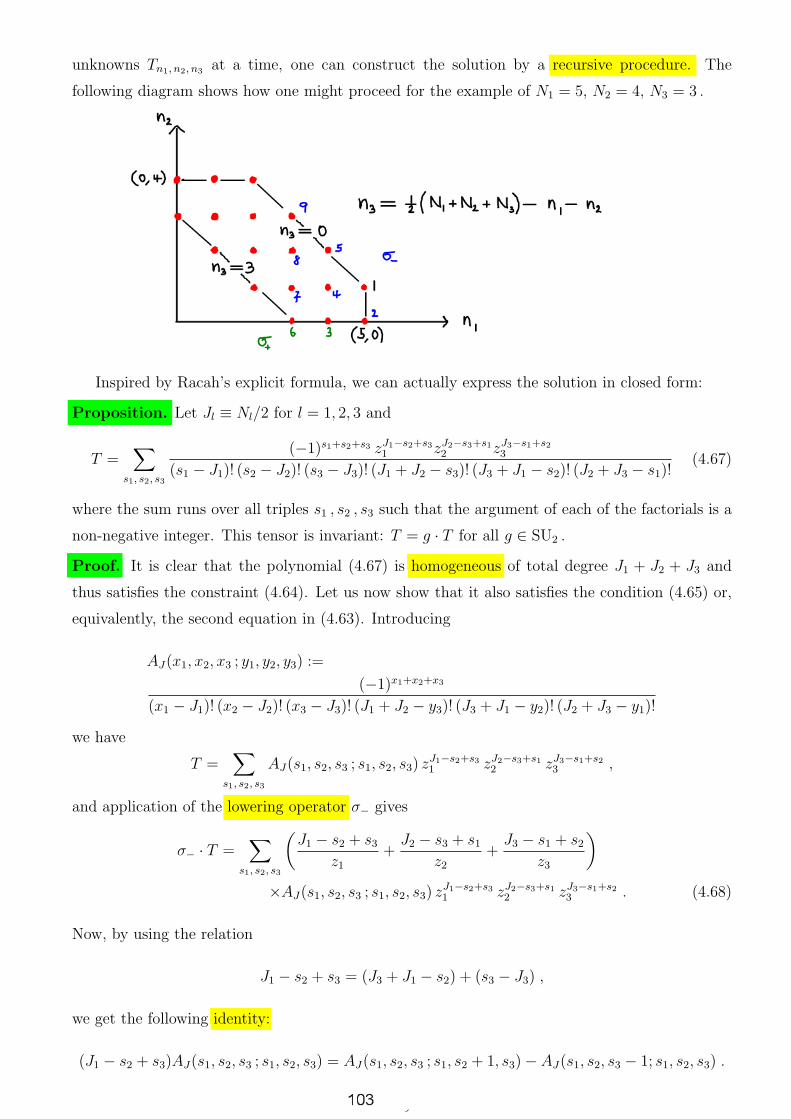
unknowns Tn1, n2, n3at a time, one can construct the solution by a recursive procedure. The
following diagram shows how one might proceed for the example of N1 = 5, N2 = 4, N3 = 3 .
Inspired by Racah’s explicit formula, we can actually express the solution in closed form:
Proposition. Let Jl ≡ Nl/2 for l = 1, 2, 3 and
T =∑
s1, s2, s3
(−1)s1+s2+s3 zJ1−s2+s3
1 zJ2−s3+s1
2 zJ3−s1+s2
3
(s1 − J1)! (s2 − J2)! (s3 − J3)! (J1 + J2 − s3)! (J3 + J1 − s2)! (J2 + J3 − s1)!(4.67)
where the sum runs over all triples s1 , s2 , s3 such that the argument of each of the factorials is a
non-negative integer. This tensor is invariant: T = g · T for all g ∈ SU2 .
Proof. It is clear that the polynomial (4.67) is homogeneous of total degree J1 + J2 + J3 and
thus satisfies the constraint (4.64). Let us now show that it also satisfies the condition (4.65) or,
equivalently, the second equation in (4.63). Introducing
AJ(x1, x2, x3 ; y1, y2, y3) :=
(−1)x1+x2+x3
(x1 − J1)! (x2 − J2)! (x3 − J3)! (J1 + J2 − y3)! (J3 + J1 − y2)! (J2 + J3 − y1)!
we have
T =∑
s1, s2, s3
AJ(s1, s2, s3 ; s1, s2, s3) zJ1−s2+s3
1 zJ2−s3+s1
2 zJ3−s1+s2
3 ,
and application of the lowering operator σ− gives
σ− · T =∑
s1, s2, s3
(
J1 − s2 + s3
z1
+J2 − s3 + s1
z2
+J3 − s1 + s2
z3
)
×AJ(s1, s2, s3 ; s1, s2, s3) zJ1−s2+s3
1 zJ2−s3+s1
2 zJ3−s1+s2
3 . (4.68)
Now, by using the relation
J1 − s2 + s3 = (J3 + J1 − s2) + (s3 − J3) ,
we get the following identity:
(J1 − s2 + s3)AJ(s1, s2, s3 ; s1, s2, s3) = AJ(s1, s2, s3 ; s1, s2 + 1, s3) − AJ(s1, s2, s3 − 1; s1, s2, s3) .
96

Two more identities of the same kind result from cyclic permutations of the index set 1, 2, 3.
Next, in (4.68) we make a shift of summation index s3 → s3 − 1 for the second term (z−12 ) and
s2 → s2 +1 for the third term (z−13 ), in order to pull out common powers of z1, z2, z3 and combine
the various contributions. In this way we recast the expression (4.68) as
σ− · T =∑
(
AJ(s1, s2, s3 ; s1, s2 + 1, s3) − AJ(s1, s2, s3 − 1; s1, s2, s3)
+AJ(s1, s2, s3 − 1; s1, s2, s3) − AJ(s1 − 1, s2, s3 − 1; s1, s2, s3 − 1)
+AJ(s1, s2 + 1, s3 ; s1 + 1, s2 + 1, s3) − AJ(s1, s2, s3 ; s1, s2 + 1, s3))
×zJ1−s2+s3−1
1 zJ2−s3+s1
2 zJ3−s1+s2
3 .
We see that the second term cancels the third one, and the first term cancels the last one. The
fourth term cancels the fifth one on making a common shift sj → sj + 1 (j = 1, 2, 3) which leaves
the powers of z1, z2, z3 unchanged. This already completes the proof that σ− · T = 0 .
Problem. By an adaptation of the calculation above, show that σ+ · T = 0 . ¤
Recall that by the choice (4.56) of Hermitian scalar product for VN , the basis vectors ϕN, n = zn
of VN have squared length
〈ϕN, n , ϕN, n〉 =
(
N
n
)−1
=n! (N − n)!
N !.
The standard practice in physics is to work with orthonormal bases. Therefore, we now introduce
the unit vectors
eJ, M :=
(
2J
J + M
)1/2
ϕ2J, J+M =
√
(2J)! ϕ2J, J+M√
(J + M)! (J − M)!∈ V2J (4.69)
for M = −J,−J + 1, . . . , J − 1, J .
Definition. Let Tn1, n2, n3≡ TN1,N2,N3
n1, n2, n3be the coefficients which are determined by comparing the
ansatz (4.62) with the solution (4.67). The Wigner 3j-symbol
(
J1 J2 J3
M1 M2 M3
)
is defined as
(
J1 J2 J3
M1 M2 M3
)
:= T 2 J1 , 2 J2 , 2 J3
J1+M1, J2+M2, J3+M3
√
(J1 J2 J3)
×√
(J1 + M1)! (J1 − M1)! (J2 + M2)! (J2 − M2)! (J3 + M3)! (J3 − M3)! (4.70)
where
(J1 J2 J3) :=(J1 + J2 − J3)! (J2 + J3 − J1)! (J3 + J1 − J2)!
(J1 + J2 + J3 + 1)!(4.71)
is called a triangle coefficient.
Remark. Note that by (4.64) the Wigner 3j-symbol vanishes unless M1 + M2 + M3 = 0 . Note
also that the Wigner 3j-symbol is just a scalar multiple of the coefficients of our tensor T given
in (4.67). The following conclusion is therefore immediate.
Corollary. The tensor
∑
M1, M2, M3
(
J1 J2 J3
M1 M2 M3
)
eJ1, M1⊗ eJ2, M2
⊗ eJ3, M3(4.72)
97

is SU2-invariant. ¤
By the isomorphism (4.53) in conjunction with the identification V ∗
N3≃ VN3
due to the invariant
pairing VN ⊗ VN → C (cf. Section 4.3.3), we finally arrive at what is called the Clebsch-Gordan
coefficient for SU2 . It is given by the formula
〈J1J2 ; M1M2 | J1J2 ; J3M3〉 := (−1)J1−J2+M3
√
2J3 + 1
(
J1 J2 J3
M1 M2 −M3
)
. (4.73)
The sign change M3 → −M3 reflects the isomorphism V ∗
N3≃ VN3
determined by the mapping
fJ3, M3→ (−1)J3−M3eJ3,−M3
(dual basis fJ, M). The remaining sign factor (−1)J1−J2−J3 is due
to what is known as the phase convention of Condon and Shortley. The normalization factor√
2J3 + 1 is motivated by the properties (4.75) and (4.76) below. A simplified notation is
〈J1J2 ; M1M2 | J1J2 ; J3M3〉 ≡ 〈J1J2M1M2 | J3M3〉 . (4.74)
The Dirac-style notation for the Clebsch-Gordan coefficient indicates that it effects a change of
orthonormal basis |J1J2 ; J3M3〉 → |J1M1〉 ⊗ |J2M2〉.
Problem. Show that the Clebsch-Gordan coefficient obeys the following relations of orthonor-
mality and completeness:
∑
M1M2
〈J1J2M1M2 | J3M3〉 〈J1J2M1M2 | J ′
3M′
3〉 = δJ3
, J ′
3δM
3, M ′
3, (4.75)
∑
J3M3
〈J1J2M1M2 | J3M3〉 〈J1J2M′
1M′
2 | J3M3〉 = δM1
, M ′
1δM
2, M ′
2. ¤ (4.76)
From an informed mathematical perspective, the Clebsch-Gordan coefficient provides us with
an SU2-equivariant homomorphism φJ1J2∈ HomSU2
(V2J3, V2J1
⊗ V2J2) by
φJ1J2(eJ3, M3
) =∑
M1+M2=M3
〈J1J2M1M2 | J3M3〉 eJ1, M1⊗ eJ2, M2
; (4.77)
thus it describes explicitly how the representation V2J3occurs in the tensor product V2J1
⊗ V2J2.
4.5 Integrals of products of Wigner D-functions
For a compact Lie group G let ρ : G → GL(V ) be an irreducible representation. Fix a basis elof V and define the matrix elements Dkl(g) of the representation by
ρ(g) el =∑
k
ek Dkl(g)
as usual. Let dg be Haar measure of G with total mass∫
Gdg = 1.
Fact. The matrix elements of an irreducible representation satisfy the orthogonality relation∫
G
Dkl(g)Dl′k′(g−1) dg =δkk′δll′
dim V. (4.78)
Proof. Applying g ∈ G to any tensor v ⊗ ϕ ∈ V ⊗ V ∗ we have
g · (v ⊗ ϕ) = ρ(g)v ⊗ ϕ ρ(g)−1.
98

The Dirac-style notation for the Clebsch-Gordan coefficient indicates that it effects a change of
orthonormal basis |J1J2 ; J3M3〉 → |J1M1〉 ⊗ |J2M2〉.
Problem. Show that the Clebsch-Gordan coefficient obeys the following relations of orthonor-
mality and completeness:
∑
M1M2
〈J1J2M1M2 | J3M3〉 〈J1J2M1M2 | J′3M
′3〉 = δJ
3, J ′
3δM
3,M ′
3, (4.75)
∑
J3M3
〈J1J2M1M2 | J3M3〉 〈J1J2M′1M
′2 | J3M3〉 = δM
1,M ′
1δM
2,M ′
2. (4.76)
From an informed mathematical perspective, the Clebsch-Gordan coefficient provides us with
an SU2-equivariant homomorphism φJ1J2 ∈ HomSU2(V2J3 , V2J1 ⊗ V2J2) by
φJ1J2(eJ3,M3) =
∑
M1+M2=M3
〈J1J2M1M2 | J3M3〉 eJ1,M1⊗ eJ2,M2
; (4.77)
thus it describes explicitly how the representation V2J3 occurs in the tensor product V2J1 ⊗ V2J2 .
4.5 Integrals of products of Wigner D-functions
For a compact Lie group G let ρ : G → GL(V ) be an irreducible representation. Fix a basis el
of V and define the matrix elements Dkl(g) of the representation by
ρ(g) el =∑
k
ek Dkl(g)
as usual. Let dg be Haar measure of G with total mass∫
Gdg = 1. In the following we will use
that fact that Haar measure is invariant under inversion, i.e.∫
Gf(g) dg =
∫
Gf(g−1) dg.
Fact. The matrix elements of an irreducible representation satisfy the orthogonality relation
∫
G
Dkl(g)Dl′k′(g−1) dg =
δkk′δll′
dimV. (4.78)
Proof. Applying g ∈ G to any tensor v ⊗ ϕ ∈ V ⊗ V ∗ we have
g · (v ⊗ ϕ) = ρ(g)v ⊗ ϕ ρ(g)−1.
The Haar average of all translates g · (v ⊗ ϕ) is a G-invariant tensor in V ⊗ V ∗. Because V is
irreducible, there exists only one such tensor; this is the canonical invariant µ−1(IdV ) =∑
ei⊗fi ;
see Eq. (4.21) of Section 4.3.1. It follows that there exists a number c(v, ϕ) ≡ c such that
∫
G
ρ(g)v ⊗ ϕ ρ(g)−1dg = c∑
i
ei ⊗ fi .
Now we specialize this relation to v = el and ϕ = fl′ and then pass to components on each side
using fk(ρ(g)el) = Dkl(g) and fl′(ρ(g)−1ek′) = Dl′k′(g
−1). The result is
∫
G
Dkl(g)Dl′k′(g−1) dg = c(el, fl′) δkk′ .
106

Next we use the invariance of Haar measure dg under inversion g 7→ g−1 to exchange the roles of
the index pairs kk′ and ll′ and infer that c(el, fl′) = c0δll′ .
The constant c0 is determined by setting k = k′, l = l′, and summing over l :
1 =
∫
G
dg =
∫
G
∑
l
Dkl(g)Dlk(g−1) dg = c0
∑
l
δll = c0 dimV,
which gives the desired result c0 = (dimV )−1.
Remark. If D(1)kl (g) and D
(2)l′k′(g
−1) are the matrix coefficients for two irreducible representations
V1 6= V2 in different isomorphism classes, then the integral∫
GD
(1)kl (g)D
(2)l′k′(g
−1) dg vanishes for all
k, l, k′, l′. Indeed, any non-zero value of the integral would imply a G-invariant tensor in V1 ⊗ V ∗2 ,
but we know from Section 4.3.1 that no such tensor exists.
From now on we restrict the discussion to the case of G = SU2 , where we use the notation
DJMN(g) ≡ fJ,M(ρJ(g) eJ,N) for the matrix elements (also known in physics as the Wigner D-
functions) of the irreducible representation of spin J . For future reference we record that
∫
SU2
DJMN(g)D
J ′
N ′M ′(g−1) dg = δJJ ′
δMM ′ δNN ′
2J + 1. (4.79)
In the remainder of this section, we are going to derive a formula for the Haar integral of a prod-
uct of three Wigner D-functions. To that end, we consider the Haar average of all SU2-translates
of some tensor X ∈ V2J1 ⊗ V2J2 ⊗ V2J3 in the tensor product of three irreducible representations
with spins J1 , J2 , J3 . Since the Haar-averaged tensor∫
(g ·X) dg is SU2-invariant and there exists
only one such tensor, namely that of Corollary (4.72), we have
∫
SU2
(g ·X) dg = c3(X)∑
M1,M2,M3
(
J1 J2 J3M1 M2 M3
)
eJ1,M1⊗ eJ2,M2
⊗ eJ3,M3,
with some unknown number c3(X) . Now let X = eJ1, N1⊗ eJ2, N2
⊗ eJ3, N3. By passing to compo-
nents with respect to the chosen basis we obtain
∫
SU2
DJ1M1N1
(g)DJ2M2N2
(g)DJ3M3N3
(g) dg = c3(eJ1, N1⊗ eJ2, N2
⊗ eJ3, N3)
(
J1 J2 J3M1 M2 M3
)
. (4.80)
Our next step is to exchange the roles of vectors and co-vectors. A quick (if dirty) way of doing
this is to take the complex conjugate of both sides of the equation and exploit the unitarity of the
representation:
DJMN(g) = DNM(g−1) .
Haar measure dg does not change under the substitution of integration variable g → g−1 (this is
an immediate consequence of Haar measure being unique). Since the Wigner 3j-symbol is real it
follows that
∫
SU2
DJ1M1N1
(g)DJ2M2N2
(g)DJ3M3N3
(g) dg = c3(eJ1,M1⊗ eJ2,M2
⊗ eJ3,M3)
(
J1 J2 J3N1 N2 N3
)
.
By comparing this with (4.80) we are led at the following conclusion.
107

Fact. For the Haar integral of a product of three Wigner D-functions one has the formula
∫
SU2
DJ1M1N1
(g)DJ2M2N2
(g)DJ3M3N3
(g) dg =
(
J1 J2 J3M1 M2 M3
)(
J1 J2 J3N1 N2 N3
)
. (4.81)
Proof. Our previous considerations imply (4.81) up to an unknown constant of proportionality.
It remains to show that this constant is unity. For that purpose we set Ml = Nl (l = 1, 2, 3) and
sum over magnetic quantum numbers. On the right-hand side we get
∑
M1M2M3
(
J1 J2 J3M1 M2 M3
)2
=∑
M3
∑
M1M2
(2J3 + 1)−1 〈J1J2M1M2 | J3 −M3〉2 =
∑
M3
(2J3 + 1)−1 = 1
from (4.73) and the orthonormality property (4.76) for the Clebsch-Gordan coefficient. To do the
integral on the left-hand side, we use the relation
χJ1(g)χJ2(g) =
J1+J2∑
J=|J1−J2|
χJ(g) , χJ(g) :=J∑
M=−J
DJMM(g) , (4.82)
which follows rather easily from
χJ(eiθσ3) =
J∑
M=−J
eiMθ =sin
(
(2J + 1)θ/2)
sin(θ/2). (4.83)
Thus our integral after summation over magnetic quantum numbers becomes
∫
SU2
χJ1(g)χJ2(g)χJ3(g) dg =
J3∑
J=|J1−J2|
∫
SU2
χJ(g)χJ3(g) dg =
∫
SU2
χJ3(g)2 dg = 1 ,
where in the last two steps we used the orthogonality (4.79).
Fact. A variant of the integral above is
∫
SU2
DJ1M1N1
(g)DJ2M2N2
(g)DJ3M3N3
(g) dg =〈J1J2M1M2 | J3M3〉 〈J1J2N1N2 | J3N3〉
2J3 + 1. (4.84)
Proof. Using completeness (4.76) of the Clebsch-Gordan coefficients we invert the relation (4.77):
eJ1, N1⊗ eJ2, N2
=∑
JN
〈J1J2N1N2 | JN〉 φJ1J2(eJ,N) .
We then apply any transformation g ∈ SU2 to obtain
∑
M1M2
eJ1,M1⊗ eJ2,M2
DJ1M1N1
(g)DJ2M2N2
(g) =∑
JNM
〈J1J2N1N2 | JN〉 φJ1J2(eJ,M)DJMN(g) .
On the right-hand side we insert the expression (4.77) for φJ1J2(eJ,M) and pass to components:
DJ1M1N1
(g)DJ2M2N2
(g) =∑
JMN
〈J1J2N1N2 | JN〉 〈J1J2M1M2 | JM〉 DJMN(g) .
Finally, we integrate both sides against DJ3M3N3
(g) = DJ3N3M3
(g−1) with Haar measure dg. The
desired result (4.84) then follows by using the orthogonality relation (4.79) on the right-hand side.
108

4.6 Tensor operators, Wigner-Eckart Theorem
Recall the action of g ∈ SU2 = Spin3 on the basis vectors eJ, M ∈ V2J of the representation for
spin J :
g · eJ, N =∑
M
eJ, M DJMN(g) .
The following definition is motivated by the quantum mechanical fact that if quantum states
transform as ψ 7→ g ψ then quantum operators transform by conjugation Op 7→ g Op g−1.
Definition. By an irreducible tensor operator of rank J one means a set of operators TJMM=−J,...,J
transforming under rotations g ∈ SU2 = Spin3 as
g TJN g−1 =∑
M
TJM DJMN(g) . (4.85)
Example. The operation of multiplying (the angular part of the wave function) by a spherical
harmonic YLM is an irreducible tensor operator of rank J = L. Important examples of tensor
operators are furnished by the problem of expanding, say, the charge density operator ρ by mul-
tipoles with respect to a distinguished point (typically the center of mass). The three (spherical)
components of the dipole part of ρ form a tensor operator of rank J = 1, the five components of
the quadrupole part of ρ form a tensor operator of rank J = 2, and so on. ¤
If Jx , Jy , Jz are the operators of total angular momentum, and J± = 1
2(Jx ± iJy), then the
infinitesimal version of (4.85) reads
[Jz , TJM ] = ~M TJM , [J± , TJM ] = ~
√
(J ∓ M)(J ± M + 1) TJ, M±1 . (4.86)
Wigner-Eckart theorem. Let TJM be (the components of) an irreducible tensor operator. Its
matrix elements between two quantum mechanical states of definite spin and spin projection are
products
〈J2M2 | TJM | J1M1〉 = 〈J1JM1M | J2M2〉 〈J1 ‖ TJ ‖ J2〉 (4.87)
of a Clebsch-Gordan coefficient and a so-called reduced matrix element.
Remark. The dependence of the matrix element on the quantum numbers M1 ,M, M2 is given
entirely by the Clebsch-Gordan coefficient. The main task (possibly difficult) in practical appli-
cations is to compute the reduced matrix element 〈J1 ‖ TJ ‖ J2〉.Proof. We begin by writing
〈J2M2 | TJM | J1M1〉 =⟨
J2M2 | g−1(
g TJM g−1)
g | J1M1
⟩
.
Then we expand g |J1M1〉 =∑ |J1N1〉 DJ1
NM(g) and
〈J2M2| g−1 = 〈g · (J2M2)| =∑
N2
〈J2N2| DJ2
N2M2(g) ,
using the unitarity of the SU2-action. We thus obtain
〈J2M2 | TJM | J1M1〉 =∑
N1N2N
〈J2N2 | TJN | J1N1〉DJ1
N1M1(g)DJ
NM(g)DJ2
N2M2(g) .
101

This result holds true for all g ∈ SU2 and remains true if we average both sides with SU2-Haar
measure. Hence, by using formula (4.84) we have
〈J2M2 | TJM | J1M1〉 = 〈J1JM1M | J2M2〉∑
N1N2N
〈J2N2 | TJN | J1N1〉〈J1JN1N | J2N2〉
2J2 + 1.
This gives the formula (4.87) of the Wigner-Eckart theorem along with an expression for the
reduced matrix element:
〈J1 ‖ TJ ‖ J2〉 = (2J2 + 1)−1∑
N1N2N
〈J2N2 | TJN | J1N1〉 〈J1JN1N | J2N2〉 . (4.88)
5 Dirac quantization condition
The original plan of this lecture course was to finish with a chapter on the foundations of quan-
tum mechanics (superposition principle: Schrodinger cat states, EPR paradox, violation of Bell’s
inequality, decoherence, many-worlds interpretation). Since there is not enough time left for a
substantial discussion of the subject, we change course and conclude with a short chapter on
another foundational theme of quantum mechanics: the quantization of electric charge.
Experimentally one observes that electric charge always occurs as an integer multiple qe = ne
(n ∈ Z) of a fundamental charge quantum e . Why nature would have it this way is not known;
the phenomenon of charge quantization is in fact one of the open questions of theoretical physics.
The situation improves, however, if there are magnetic charges. Allowing for the existence of
magnetic monopoles, Dirac (1931) argued that quantum mechanics is consistent if and only if the
product of any pair qe , qm of electric and magnetic charges is an integer multiple of 2π~ :
qe qm ∈ 2π~ Z . (5.1)
This condition, known as the Dirac quantization condition, can be read in two directions. Given
a smallest magnetic charge µ , it quantizes the electric charge according to qe ∈ (2π~/µ) Z .
Conversely, given an electric charge quantum e , magnetic charge is quantized by qm ∈ (2π~/e) Z .
The goal of the present chapter is to offer some physical heuristics and mathematical back-
ground for the Dirac quantization condition (5.1). Please be advised that this story, albeit a corner
stone of theoretical physics, is speculative in the context of physics as an experimental science, as
magnetic monopoles have never been observed in the laboratory to this day. [However, quoting
string theorist J. Polchinski (arXiv:hep-th/0304042): “the existence of magnetic monopoles seems
like one of the safest bets that one can make about physics not yet seen”.]
To begin, here is how the equations of electrodynamics (in traditional vector notation) would
have to look for a non-zero magnetic charge density ρm and magnetic current density jm :
rotH = D + je , div D = ρe , D = ε0 E , (5.2)
−rotE = B + jm , div B = ρm, B = µ0 H . (5.3)
102