lectures on advance macroeconomics - emilio cuilty · 1 my lectures are written to my students....
TRANSCRIPT

Lectures on Advance Macroeconomics
Emilio Cuilty Luna
March 28, 2013

1
My lectures are written to my students. Please talk to me before circulating the notes. I deeply appreciate allcomments and help to improve these lecture notes.
Syllabus
Objective: The main purpose of this course is to review the economic uctuations, review the ideas from the neo-classic and Neokeynesian schools and nally attempt to give some behavioral explanations. The quantitativemathematical or analytical requirements are very high, some review will be given on relevant tools for solveproblems nevertheless advanced calculus, econometrics and dynamic programming will be assumed. Howeverthe intuition will be the most important part to develop. The core of the course will be centered in Romer'sbook; from time to time it will be necessarily to review other texts such as Stokey and Lucas or Summers'papers. At the end of the course the approved student will understand the dierences in the explanations ofboth schools and how to solve standard problems of macroeconomic uctuations. The student will also beable give clean proofs of the theorems or nd the relevant results of the models.
Approve: This course is far from being an easy course, and probably will consume an important part of your timeduring the semester. My recommendation to approve the course is to study a lot. It is almost impossible toapprove just reading the class notes. HARD WORK is required to approve. It is expected that the studentwill read the relevant chapter of the book at least once before entering the classroom, more readings will beneeded to complete homework or to fully understand the theory.
Ethics: I believe that as future economists you should always be guided by social norms and ethic codes. Accordingto the former idea you might NEVER cheat or copy in a homework, exam or whatever. Those students failingto behave honestly will be punished with an automatic D.A. with no consideration to negotiate. My gradingscheme is designed to fail anyone that receives a D.A., so please don't try to make tricks on me. It is importantto be respectful with others ideas, please be kind with everybody questions and pay attention to all ideas,they might appear on the exams or quizzes.
Grading scheme
• Two Partial exams, 60% of the nal grade
• Final evaluation, 30% of the nal grade
• 6 or 5 quizzes, 10% of the nal grade
• Bonus, extra 10% and will be only available for 2 or 3 students
Exams: The rst partial exam will be on February 14, the second partial exam will be on April 4 and the nalevaluation will be on May 9. These dates are xed and I will not move any exam for any reason. So if youhave more than one exam this day I suggest to you to try to move the other exam(s), otherwise good luck.Both partial exams cover all the topics we review in class or in the Problem Sets. The second partial examcovers the topics of the second partial and the rst one. The nal evaluation will comprehend only the secondpartial and the last topics covered.
Quizzes: There will be 5 or 6 surprise quizzes. The quizzes will be one or two short questions about the materialcovered last week. The quizzes will be applied at 7:07 with a maximum length of 10 minutes. If you arrivelater than 7:17 you will not have access to the quiz and will count as zero. Nevertheless you should come toclass even if you miss the quiz, otherwise you will miss important material.
Problem-Sets: There will be 4 or 5 problem sets. The problem sets are complicated and will require a lot oftime to complete them, so start them as soon as possible. You might work in groups, pairs or whatever.The problem sets do not account for any points on the nal grade, however not completing them will be adangerous move, in order to master theory you need to work, fail, and rethink. Problem Sets will be answeredin a class lecture, however you must present your Problem Set at the beginning of the session otherwise youwill be not allowed to enter.
Bonus: I do not yet how to account for bonus, nevertheless I will think about it.

2
Topics
• Introduction, Where is the State of the Macro today?
Krugman, P. How Did Economists Get It So Wrong? (2009), New York Times
• Real-Business-Cycle Theory, The freshwater's new hope
Romer, D. Advance Macroeconomics (2012) McGraw-Hill 4th edition. Chapter 5
Mankiw, G. Macroeconomics (2000) 4th edition. Chapter 19
Stokey, N. and R. Lucas Recursive Methods in Economics Dynamics Harvard Press 1th edition. Chap-ters 4, 5, 6
• Nominal Rigidity, The Neokeynesian strikes back
Romer, D. Advance Macroeconomics (2012) McGraw-Hill 4th edition. Chapter 6
• Dynamic Stochastic General Equilibrium Models of Fluctuation, The return of the Neoclassic school
Romer, D. Advance Macroeconomics (2012) McGraw-Hill 4th edition. Chapter 7
Mas-Colell,A., M. Whinston and J. Green, Microeconomic Theory (1995) Oxford Press 1th edition.Chapters 16 and 19
Stokey, N. and R. Lucas Recursive Methods in Economics Dynamics Harvard Press 1th edition. Chap-ters 9 and 10
• Behavioral Finance and Behavioral Macroeconomics. Get rid of that non sense
Long, J. B. D., A. Shleifer, L. H. Summers, and R. J. Waldmann (1991): The Survival of Noise Tradersin Financial Markets, The Journal of Business, 64(1), pp. 119.

Part I
Introduction
3

Chapter 1
Where is the state of the Macro today?
1.1 A clever discussion of Macroeconomics.
In September of 2009 the Nobel laureate Paul Krugman published an interesting article in the New York Times,How Did Economists Get It So Wrong?. This rst class we are going to review the most important points ofthe article. Hopefully at the end of the class you will understand better why is important to dig deeper in tomacroeconomics (and why society expects from you to complete several courses on macro) even if history hasshowed us that this science do not work at all. Most of you may not remember but when I was a student, hereat ITESM, the academic economic society were congratulating them self on how they had fully understood howmacroeconomics work. In fact Oliver Blanchard of M.I.T. declared that the state of the Macro was good, and theeternal ght between neoclassic school and neokeynesian view ended with an almost perfect discipline. Thanks tothe well designed public policy the most important economy (yes, the United States of America) had experienceda period of bonanza, called the great moderation. Even Mexico, back in 2006, was a promising economy, with acentral bank taking care of ination and a new nice government ghting economic recessions.
But as Krugman mentions, in 2008 everything came apart.
The economic-nancial-debt-or whatever crisis of 2008 was not predicted by almost anyone, even if old Ben Bernankewas on guard 24 7. However Krugman argues that this is not the biggest problem. The big issue with the eldof macroeconomics is the blindness of the profession, the dogma in the great market and the nice touch of thegovernment. Krugman believes that the economics profession went astray because economists, as a group, mistookbeauty, clad in impressive-looking mathematics, for truth.
I believe that most sciences work when there is no problem surrounding them. Nevertheless when the societyfaces an euro zone in crisis and America with almost a zero interest rate!(leaving no room to monetary policy)the scientic community search for a change (a quick, cheap and beautiful change). In the words of KrugmanUnfortunately, this romanticized and sanitized vision of the economy led most economists to ignore all the thingsthat can go wrong. They turned a blind eye to the limitations of human rationality that often lead to bubbles andbusts; to the problems of institutions that run amok; to the imperfections of markets especially nancial markets that can cause the economy's operating system to undergo sudden, unpredictable crashes; and to the dangerscreated when regulators don't believe in regulation.
1.1.1 From Smith to Keynes and Back
I do believe that you believe as society believes that economics was created by Adam Smith, in the 1776 famousbook The Wealth of the Nations. The central (macro) message of the Wealth of the Nations and the next 160 yearsof research was TRUST THE MARKET!. In 1844 was published the novel by Alexander Dumas the count of MonteCristo. You might remember that the count decided to study economics to become a successful man, because backthere those whom studied economics (i.e. The Wealth of the Nations) will understand better the market and couldtake advantages from it. Nevertheless in 1929 something went wrong with the market, destroying everything ourold friend from Monte Cristo believed. Some years later in the book of Macroeconomics of Parking, the author
4

CHAPTER 1. WHERE IS THE STATE OF THE MACRO TODAY? 5
claims that economist are the clever guys in the world because they know how to live with limited resources and tobe happy with them, we haven't learn anything.
According to Krugman besides what you have heard, Keynes did not wanted to live in world with a governmenttaking care of everybody. He described his analysis in his 1936 masterwork, The General Theory of Employment,Interest and Money, as moderately conservative in its implications. He wanted to x capitalism, not replace it.The truth about the general theory is the fact that government can, and should make intervention when some shockor depression haunts the nation. Here at the ITESM you have previously review some important implications aboutKeynes. Most of them are found in the book of Mankiw.
Then Milton Friedman arrived, with the new monetarism doctrine. Monetarists did not disagree with the ideathat government should make interventions, in fact Friedman once sated We are all Keynesians now, howeverthe government should only take care of eliminate externalities, instructing central banks to keep and the nation'smoney supply, the sum of cash in circulation and bank deposits, growing on a steady path. There is a great greatbook that you should read whenever you have some extra time called Capitalism and Freedoms by Friedman.
Eventually, however, the anti-Keynesian counterrevolution went far beyond Friedman's position, which came toseem relatively moderate compared with what his successors were saying. Among nancial economists, Keynes'sdisparaging vision of nancial markets as a casino was replaced by ecient market theory, which asserted thatnancial markets always get asset prices right given the available information (this means that no one will everpay more than the ecient price for an action or a bound, in other words those LAFS and LEFs from ITESM willalways charge the optimum for every stock, bond or whatever)
Not all macroeconomists were willing to go down this road: many became self-described New Keynesians, whocontinued to believe in an active role for the government. Yet even they mostly accepted the notion that investorsand consumers are rational and that markets generally get it right (Krugman is one of those). Not everyone wasa Keynesian or a neoclassic, there were a few that believed that humans were not perfect machines, and thatrationality might not hold in the nancial markets, but they were ghting against the tide. If you want to knowmore about them, you should read papers of Schlifer,Labison, and some of Summers.
1.1.2 Panglossian Finance
According to Keynes the nancial markets can be understood as beauty contests. In order to understand them youmust not pick your favorite girl, but the one you believe will be the favorite of the jury. Nevertheless in the 70's thenancial world was understood as perfect, we humans have nothing to worry about bubbles, investors irrationalityand destructive speculation. Fama's hypothesis dominated the theory, this theory claims that the price you see onan stock is exactly the true value of the company given the information of the company's earnings. According toKrugman some Harvard economists believe in Fama so blind that their recommendation was to maximize the stockprices of a company for a better economy.
I am pretty sure you remember the CAPM model. It is a beautiful model with very nice implications, how to valuean asset and how to put a price to almost every derivative. But it only works in the scheme of ecient markets, soin my opinion does not work. Krugman argues that nancial economist rarely asked themselves if the price actuallyreected the world fundamentals. Instead they asked if the asset prices reected the other asset prices. Summersviewed nancial economist as ketchup economist, if a two quarts bottle sell invariable for exactly as twice as muchof a quart bottle of ketchup then the market is ecient.
According to Krugman with the mocks and everything, nothing change. At that time Greenspan who was then theFed chairman and a long-time supporter of nancial deregulation whose rejection of calls to rein in sub prime lendingor address the ever-inating housing bubble rested in large part on the belief that modern nancial economicshad everything under control. By October of last year, however, Greenspan was admitting that he was in astate of shocked disbelief, because the whole intellectual edice had collapsed.What should policy makersdo? Unfortunately, macroeconomics, which should have been providing clear guidance about how to address theslumping economy, was in its own state of disarray

CHAPTER 1. WHERE IS THE STATE OF THE MACRO TODAY? 6
1.1.3 The Trouble with Macro
Consider the travails of the Capitol Hill Baby-Sitting Co-op. This co-op, whose problems were recounted in a 1977article in The Journal of Money, Credit and Banking, was an association of about 150 young couples who agreed tohelp one another by baby-sitting for one another's children when parents wanted a night out. To ensure that everycouple did its fair share of baby-sitting, the co-op introduced a form of scrip: coupons made out of heavy pieces ofpaper, each entitling the bearer to one half-hour of sitting time. Initially, members received 20 coupons on joiningand were required to return the same amount on departing the group.
Unfortunately, it turned out that the co-op's members, on average, wanted to hold a reserve of more than 20coupons, perhaps, in case they should want to go out several times in a row. As a result, relatively few peoplewanted to spend their scrip and go out, while many wanted to baby-sit so they could add to their hoard. Butsince baby-sitting opportunities arise only when someone goes out for the night, this meant that baby-sitting jobswere hard to nd, which made members of the co-op even more reluctant to go out, making baby-sitting jobs evenscarcer. . . .In short, the co-op fell into a recession
The question is whether this particular example, in which a recession is a problem of inadequate demand thereisn't enough demand for baby-sitting to provide jobs for everyone who wants one gets at the essence of whathappens in a recession.
Forty years ago most economists would have agreed with this interpretation. But since then macroeconomics hasdivided into two great factions: saltwater economists (mainly in coastal U.S. universities), who have a more orless Keynesian vision of what recessions are all about; and freshwater economists (mainly at inland schools), whoconsider that vision nonsense.
Freshwater economist are those who does not believe in this explanation. The central fact is that markets work, sothere cannot be a lack of demand, because prices always move to match supply and demand. If people want morecoupons the price will rise. So why we see that there is unemployment in recessions?
In the 1970s the leading freshwater macroeconomist, the Nobel laureate Robert Lucas, argued that recessions werecaused by temporary confusion: workers and companies had trouble distinguishing overall changes in the level ofprices because of ination or deation from changes in their own particular business situation. And Lucas warnedthat any attempt to ght the business cycle would be counterproductive: activist policies, he argued, would justadd to the confusion.
Edward Prescott, who was then at the University of Minnesota, argued that price uctuations and changes indemand actually had nothing to do with the business cycle. Rather, the business cycle reects uctuations in therate of technological progress, which are amplied by the rational response of workers, who voluntarily work morewhen the environment is favorable and less when it's unfavorable. Unemployment is a deliberate decision by workersto take time o.
But the basic premise of Prescott's real business cycle theory was embedded in ingeniously constructed mathe-matical models, which were mapped onto real data using sophisticated statistical techniques, and the theory cameto dominate the teaching of macroeconomics in many university departments. In 2004, reecting the theory'sinuence, Prescott shared a Nobel with Finn Kydland of Carnegie Mellon University.
On the other side Saltwater economists believe that the demand side explanation was too compelling to reject.N. Gregory Mankiw at Harvard, Olivier Blanchard at M.I.T. and David Romer at the University of California,Berkeley and of course Paul Krugman of M.I.T. were trying to add enough imperfections to accommodate a moreor less Keynesian view of recessions, so active policy to ght recessions remained desirable.
But the self-described New Keynesian economists weren't immune to the charms of rational individuals and perfectmarkets. They tried to keep their deviations from neoclassical orthodoxy as limited as possible. This meant thatthere was no room in the prevailing models for such things as bubbles and banking-system collapse.

CHAPTER 1. WHERE IS THE STATE OF THE MACRO TODAY? 7
Nevertheless around 1985 and 2007 the ght was only about theory and not about policy making. New Keynesians,unlike the original Keynesians, didn't think scal policy changes in government spending or taxes was neededto ght recessions. They believed that monetary policy, administered by the technocrats at the Fed, could providewhatever remedies the economy needed. At a 90th birthday celebration for Milton Friedman, Ben Bernanke,formerly a more or less New Keynesian professor at Princeton, and by then a member of the Fed's governing board,declared of the Great Depression: You're right. We did it. We're very sorry. But thanks to you, it won't happenagain. The clear message was that all you need to avoid depressions is a smarter Fed. freshwater economists foundlittle to complain about. (They didn't believe that monetary policy did any good, but they didn't believe it didany harm, either.)
1.1.4 Nobody could have predicted...
It's what you say with regard to disasters that could have been predicted, should have been predicted and actuallywere predicted by a few economists who were scoed at for their pains. Robert Shiller did a prediction of thebubble the house market. But policy maker did not see anything, Carstens among them. Home price increases,Ben Bernanke said in 2005, largely reect strong economic fundamentals. Agustin Carstens limited to say thatMexico will suer only from a Catarrito.
Eugene Fama, the father of the ecient-market hypothesis, declared that the word `bubble' drives me nuts, andwent on to explain why we can trust the housing market: Housing markets are less liquid, but people are verycareful when they buy houses. It's typically the biggest investment they're going to make, so they look around verycarefully and they compare prices. The bidding process is very detailed. Yes people compared prices, but amongother bad prices, just ketchup economics again.
U.S. households have seen $13 trillion in wealth evaporate. More than six million jobs have been lost, and theunemployment rate appears headed for its highest level since 1940. So what guidance does modern economics haveto oer in our current predicament? And should we trust it?
1.1.5 The Stimulus Squabble
the crisis ended the phony peace. Suddenly the narrow, technocratic policies both sides were willing to accept wereno longer sucient and the need for a broader policy response brought the old conicts out into the open, ercerthan ever.
The Fed dealt with the recession that began in 1990 by driving short-term interest rates from 9 percent down to3 percent. It dealt with the recession that began in 2001 by driving rates from 6.5 percent to 1 percent. And ittried to deal with the current recession by driving rates down from 5.25 percent to zero. But zero, it turned out,isn't low enough to end this recession. And the Fed can't push rates below zero, since at near-zero rates investorssimply hoard cash rather than lending it out.
Fiscal stimulus is the Keynesian answer to the kind of depression-type economic situation we're currently in. SuchKeynesian thinking underlies the Obama administration's economic policies and the freshwater economists arefurious.Chicago's Cochrane, outraged at the idea that government spending could mitigate the latest recession,declared: It's not part of what anybody has taught graduate students since the 1960s. They [Keynesian ideas]are fairy tales that have been proved false. It is very comforting in times of stress to go back to the fairy tales weheard as children, but it doesn't make them less false. (It's a mark of how deep the division between saltwater andfreshwater runs that Cochrane doesn't believe that anybody teaches ideas that are, in fact, taught in places likePrinceton, M.I.T. and Harvard.)
Yet if the crisis has pushed freshwater economists into absurdity, it has also created a lot of soul-searching amongsaltwater economists. Their framework, unlike that of the Chicago School, both allows for the possibility of invol-untary unemployment and considers it a bad thing. But the New Keynesian models that have come to dominateteaching and research assume that people are perfectly rational and nancial markets are perfectly ecient. Toget anything like the current slump into their models, New Keynesians are forced to introduce some kind of fudgefactor that for reasons unspecied temporarily depresses private spending. (I've done exactly that in some of my

CHAPTER 1. WHERE IS THE STATE OF THE MACRO TODAY? 8
own work.) And if the analysis of where we are now rests on this fudge factor, how much condence can we havein the models' predictions about where we are going?
The state of macro, in short, is not good. So where does the profession go from here?
1.1.6 Flaws and Frictions
According to Krugman this should be the future of nance, and I do believe it too.
The good news is that we don't have to start from scratch. Even during the heyday of perfect-market economics,there was a lot of work done on the ways in which the real economy deviated from the theoretical ideal. Thereis work on behavioral nance. First, many real-world investors bear little resemblance to the cool calculators ofecient-market theory: they're all too subject to herd behavior, to bouts of irrational exuberance and unwarrantedpanic. Second, even those who try to base their decisions on cool calculation often nd that they can't, thatproblems of trust, credibility and limited collateral force them to run with the herd.
Larry Summers once began a paper on nance by declaring: THERE ARE IDIOTS. Look around. But what kindof idiots (the preferred term in the academic literature, actually, is noise traders) are we talking about? Behavioralnance, drawing on the broader movement known as behavioral economics, tries to answer that question by relatingthe apparent irrationality of investors to known biases in human cognition, like the tendency to care more aboutsmall losses than small gains or the tendency to extrapolate too readily from small samples (e.g., assuming thatbecause home prices rose in the past few years, they'll keep on rising).
1.1.7 Re-Embracing Keynes
Here are the last recommendations from Krugman, First admit that nancial markets fall far short of perfection,Second, they have to admit and this will be very hard for the people who giggled and whispered over Keynes that Keynesian economics remains the best framework we have for making sense of recessions and depressions.Third, they'll have to do their best to incorporate the realities of nance into macroeconomics.
1.1.8 So why study macro and old ideas?
I have to admit that I am not fully convinced with the vision of Krugman, nor I am Neokeynesian or a Neoclassic.Nevertheless I do believe that in order to save the Macro we must understand what is wrong with it. To understandwhat is wrong with the macro we need to master its foundations and try to attack them. I believe society hashope on young economist to came with a solution, there is plenty work to do. In contrast with microeconomics,macroeconomics needs young people to recreate the eld. This course will be a review of the models that explaineconomic uctuations according to both schools neoclassic and Neokeynesian. Maybe if we have time we will reviewsomething about behavioral nance at the intuition, Welcome to Advance Macroeconomics II, all resemble withreality is merely coincidence, really coincidence.

Chapter 2
Real-Business-Cycle Theory, The
freshwater's new hope
2.1 A Beginners Model
Assumptions
• The economy is formed by identical consumers (households) and a number of identical rms. Everyone isprice taker, so we are under perfect competition
• Consumers live forever
• There are only 3 production inputs: capital K, Labor L and Technology A
Production
The production in the economy is described by a Cobb-Douglas function
Yt = Kαt (LtAt)
1−α
where 0 < α < 1
All the production is divided in Consumption C, Investment I and Government Purchases G
Yt = Gt + Ct + It
Each period the capital is depreciated by a constant fraction of δ
Kt+1 = Kt + It − δKt
Or in other wordsKt+1 = Kt + Yt −Gt − Ct − δKt
Wage as usual is equal to the marginal labor productivity aYtaLt = (1−α)Kα
t (LtAt)−αAt = (1−α)
(KtLt
)αA1−αt = w.
Equally the capital is paid by the marginal productivity. aYtaKt = α
(LtAtKt
)1−α= rt + δ
Household
The representative household maximize the expected value of
U =
∞∑t=0
e−ρtu(ct, 1− lt)NtH
9

CHAPTER 2. REAL-BUSINESS-CYCLE THEORY, THE FRESHWATER'S NEW HOPE 10
Most of the times when we are talking about discrete time it is expected to use for discount 1(1+ρ)t , nevertheless
the model is log-linear so it will be useful to use an exponential discount.
u()is the instant utility function and ρ is the discount rate. Nt is the population and H is the number of households.Then by the rst assumption it follows that Nt
H is the number of members of the household.
We will assume that the populations grows to a constant rate n and for stability reasons n < δ
LnNt = N + nt
Or in other words Nt = eN+nt where N is the initial level of the population
As you can see the utility function of the households depends on c the consumption per member and 1 − lt theleisure per member. Given the rst assumption c = C
N and l = LN . For simplicity we will additional assume a utility
function log-linearut = Lnct + bln(1− lt)
where b > 0
Technology and Government
In absence of shocks the technology will grow as LnAt = At+gt where gT is constant. Nevertheless we will introduce
a stochastic shock then LnAt = At + gt + At where At is an auto-regressive process of order 1. At = ρAAt−1 + εA,t.Where εA,t is a white noise and −1 < ρa < 1.
The government purchases are paid by lump-sum taxes, and they can be described as follow:
LnGt = G + (n + g)t + Gt where Gt = ρGGt−1 + εG,t. Where εG,t is a white noise not correlated with εA,t and-1<ρG<1, this concludes the model.
Review
Denition 1. Stochastic ProcessGiven (Ω,Γ, %) probability space a Stochastic Process is an index process of random variables xtt∈Z where τ
is the set of indexes
a
Denition 2. White NoiseGiven (Ω,Γ, %) probability space, a succession of εtt∈Z is a white noise if and only if
1. ∨t, s cov(εt, εs) = 0 and s 6= t
2. ∨t E(εt) = 0
3. ∨t var(εt) = σ2 <∞
2.2 The households behavior
One Period
Lets start assuming the household only lives one period and does not posses an initial wealth. For simplicity assumeonly one member per household. The problem of the household then is:
Max
U = Lnc+ bLn(1− l)
s.a. c = wl
CHAPTER 2. REAL-BUSINESS-CYCLE THEORY, THE FRESHWATER'S NEW HOPE 11
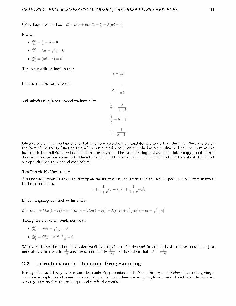
Using Lagrange method L = Lnc+ bLn(1− l) + λ(wl − c)
F.O.C.
• ∂L∂c = 1
c − λ = 0
• ∂L∂l = λw − b
1−l = 0
• ∂L∂λ = (wl − c) = 0
The last condition implies thatc = wl
then by the rst we have that
λ =1
wl
and substituting in the second we have that1
l=
b
1− l
1
l= b+ 1
l =1
b+ 1
Observe two things, the rst one is that when b is zero the individual decides to work all the time. Nevertheless bythe form of the utility function this will be an explosive solution and the indirect utility will be −∞. b measureshow much the individual values the leisure over work. The second thing is that in the labor supply and leisuredemand the wage has no impact. The intuition behind this idea is that the income eect and the substitution eectare opposite and they cancel each other.
Two Periods No Uncertainty
Assume two periods and no uncertainty on the interest rate or the wage in the second period. The new restrictionto the household is
c1 +1
1 + rc2 = w1l1 +
1
1 + rw2l2
By the Lagrange method we have that
L = Lnc1 + bLn(1− l1) + e−ρ[Lnc2 + bLn(1− l2)] + λ[w1l1 + 11+rw2l2 − c1 − 1
1+r c2]
Taking the rst order conditions of l′s
• ∂L∂l1
= λw1 − b1−l1 = 0
• ∂L∂l2
= λw2
1+r − e−ρ b
1−l2 = 0
We could derive the other rst order conditions to obtain the demand functions, both to save some time justmultiply the rst one by 1
w1and the second one by 1+r
w2. we have then that λ = b
1−l1
2.3 Introduction to Dynamic Programming
Perhaps the easiest way to introduce Dynamic Programming is like Nancy Stokey and Robert Lucas do, giving aconcrete example. So lets consider a simple growth model, here we are going to set aside the intuition because weare only interested in the technique and not in the results.

CHAPTER 2. REAL-BUSINESS-CYCLE THEORY, THE FRESHWATER'S NEW HOPE 12
The growth model, the deterministic scenario
Assumptions
A nite number of Identical Households that live forever
Each period only a good is produced yt with two inputs capital kt and labor lt
The production function is yt = F (kt, lt) and is divided into consumption and savings
ct + it ≤ yt = F (kt, lt)
F (kt, lt) is continuously dierentiable, strictly increasing, strictly quasi concave and homogeneous of degree 1 with
• F (0, l) = 0
• Fk(k, n) > 0
• Fn(k, n) > 0
• For all k, n > 0
limk→∞Fk(k, 1) = 0 and limk→0Fk(k, 1) =∞
The only decision the household has to make is how much to consume and save. The capital depreciates to aconstant rate of −1 < δ < 1
kt+1 = (1− δ)kt + it
Finally the preferences over consumption have the form of
∞∑t=0
βtU(ct) 0 < β < 1
Assume also that the population is constant over time and normalize the labor force to 1. The labor supply mustsatisfy 0 ≤ l ≤ 1 all t
Rewriting (for reducing the number of variables) the rst restriction as
ct + kt+1 − (1− δ)kt ≤ F (kt, lt) all t (1)
The households have identical preferences over time and they have an additive form
u(c0, c1, ...) =
∞∑t=0
βtU(ct) (2)
The utility of the period t U : R+ → R is bounded, continuously dierentiable, strictly increasing and strictlyconcave. Limc→0U
′(c) =∞. Households do not value leisure.
2.3.1 The Problem in Sequence Form
Consider the problem of the social planer which objective is to maximize (2), this is achieved by choosing sequences(ct, kt, lt)∞t=0 constrained by feasible restrictions given k0 > 0
Observe that in the optimum the product will not be wasted. This means that 1 can be written with equality. Wecan simplify ct by substituting the former idea on the utility function. Given the fact that leisure is not valued andthat Fl(kt, lt) > 0 is obvious that l = 1 .Then we can say that kt and yt are the production and capital per worker,but also the total production and the total capital. It is convenient to dene
f(k) = F (k, 1) + (1− δ)k (3)

CHAPTER 2. REAL-BUSINESS-CYCLE THEORY, THE FRESHWATER'S NEW HOPE 13
As the total supply of goods in the economy, including the not depreciated capital in the current period
The social planner problem is thenMax
(kt+1)∞t=0
∞∑t=0
βtU(f(kt)− kt+1)
s.t. 0 ≤ kt+1 ≤ f(kt) t = 0, 1, ...
k0 > 0
It will be useful to start this example with the nite horizon case
Max
(kt+1)Tt=0
T∑t=0
βtU(f(kt)− kt+1)
s.t. 0 ≤ kt+1 ≤ f(kt) t = 0, 1, ...T (4)
k0 > 0
The sequences (kt+1)Tt=0 are a close set, bounded and a convex set of RT+1. Additionally note that the objectivefunction is continuous and strictly concave. By the Kuhn-Tucker uniqueness conditions the former idea implies thatthe problem has an unique solution. To obtain the conditions observe that f(0) = 0 and that U ′(0) = ∞, thenthe (4) set of restrictions do not bind except for kT+1. It must be true that kT+1 = 0
Then the solutions must satisfy
βf ′(kt)U [f(kt)− kt+1] = U ′[f(kt−1)− kt] (5)
kT+1 = 0 (6)
k0 > 0 given
Example 3. Let f(k) = kα, 0 < α < 1 and U(c) = ln(c). Write down equation 5, then apply a change of varibalezt = kt
kαt−1to turn the result in a dierence equation of order 1 in zt
We know that U(ct) = ln(ct), then U′(ct) = 1
ct. Substituting what we know about consumptionU ′(f(kt)− kt+1) =
1kαt −kt+1
. Then it must be true that equation ve is
βαkα−1t
1
kαt − kt+1=
1
kαt−1 − kT
Rearranging the terms we have kαt − kt+1 = αβ(kαt−1 − kt)kα−1t , then divide everything by kαt
1− kt+1
kt= αβ(kαt−1 − kt)k−1t
or
1− zt+1 = αβ(1
zt− 1)
Finally
zt+1 = 1− αβ(1
zt− 1)
Example 4. Imagine that zt has reached the stable state (this is only true in the long long run), nd the stable(s)state(s)

CHAPTER 2. REAL-BUSINESS-CYCLE THEORY, THE FRESHWATER'S NEW HOPE 14
It must be true that zt = zt+1 = z in the steady state, so from the last equation we have that
z = 1 + αβ − αβ
z
Then solving for z
z2 − (1 + αβ)z + αβ = 0
By the general formula we have that z1 = 1 and z2 = αβ
Example 5. There must be only one solution to the problem, in fact the condition (6) implies that kT+1 = 0 whichmeans zT+1 = 0
kαt= 0. Find the solution to the dierence equation recursively from zT+1 = 0,
We know that zt+1 = 1− αβ( 1zt− 1), solving for zt
zt+1 − 1
αβ= 1− 1
zt
zt =αβ
αβ − zt+1 + 1
Given the fact that zT+1 = 0 in time T , then
zT =αβ
αβ + 1
Now if we take the problem to the time T − 1.
zT−1 =αβ
(αβ − zt + 1)=
αβ
(αβ − αβαβ+1 + 1)
=αβ(αβ + 1)
αβ2 + αβ − αβ + αβ + 1
zT−1 =αβ(αβ + 1)
(αβ)2 + αβ + 1
Now lets nd T − 2
zT−2 =αβ
(αβ − zt−1 + 1)=
αβ
(αβ − αβ(αβ+1)(αβ)2+αβ+1 + 1)
=αβ((αβ)2 + αβ + 1)
((αβ)3 + (αβ)2 + αβ + 1)
In general for time T − i
ZT−i =αβ(1 + αβ + ...+ (αβ)i)
(1 + αβ + ...+ (αβ)i + (αβ)i+1)
And if we say that i = T − t
zT−T+t = zt =αβ(1 + αβ + ...+ (αβ)T−t)
(1 + αβ + ...+ (αβ)i + (αβ)T−t+1)
To simplify this expression lets say S ≡ (1+αβ+...+(αβ)T−t) then it must be that αβS = (αβ+...+(αβ)T−t+1).S − αβS = (1− (αβ)T−t+1)
S =(1− (αβ)T−t+1)
1− αβThen
zt =αβ( (1−(αβ)T−t+1)
1−αβ )
(1−(αβ)T−t+2)1−αβ
=αβ(1− (αβ)T−t+1)
(1− αβT−t+2)
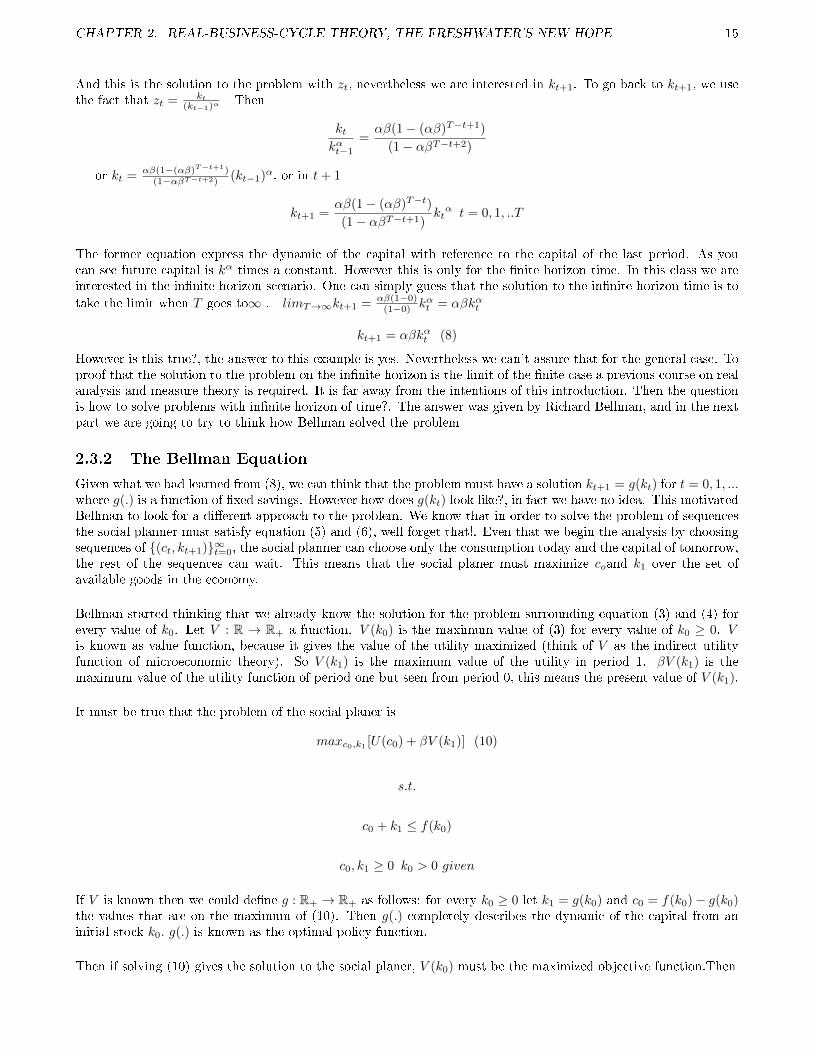
CHAPTER 2. REAL-BUSINESS-CYCLE THEORY, THE FRESHWATER'S NEW HOPE 15
And this is the solution to the problem with zt, nevertheless we are interested in kt+1. To go back to kt+1, we usethe fact that zt = kt
(kt−1)αThen
ktkαt−1
=αβ(1− (αβ)T−t+1)
(1− αβT−t+2)
or kt = αβ(1−(αβ)T−t+1)(1−αβT−t+2)
(kt−1)α, or in t+ 1
kt+1 =αβ(1− (αβ)T−t)
(1− αβT−t+1)ktα t = 0, 1, ..T
The former equation express the dynamic of the capital with reference to the capital of the last period. As youcan see future capital is kα times a constant. However this is only for the nite horizon time. In this class we areinterested in the innite horizon scenario. One can simply guess that the solution to the innite horizon time is to
take the limit when T goes to∞ . limT→∞kt+1 = αβ(1−0)(1−0) kαt = αβkαt
kt+1 = αβkαt (8)
However is this true?, the answer to this example is yes. Nevertheless we can't assure that for the general case. Toproof that the solution to the problem on the innite horizon is the limit of the nite case a previous course on realanalysis and measure theory is required. It is far away from the intentions of this introduction. Then the questionis how to solve problems with innite horizon of time?. The answer was given by Richard Bellman, and in the nextpart we are going to try to think how Bellman solved the problem
2.3.2 The Bellman Equation
Given what we had learned from (8), we can think that the problem must have a solution kt+1 = g(kt) for t = 0, 1, ...where g(.) is a function of xed savings. However how does g(kt) look like?, in fact we have no idea. This motivatedBellman to look for a dierent approach to the problem. We know that in order to solve the problem of sequencesthe social planner must satisfy equation (5) and (6), well forget that!. Even that we begin the analysis by choosingsequences of (ct, kt+1)∞t=0, the social planner can choose only the consumption today and the capital of tomorrow,the rest of the sequences can wait. This means that the social planer must maximize coand k1 over the set ofavailable goods in the economy.
Bellman started thinking that we already know the solution for the problem surrounding equation (3) and (4) forevery value of k0. Let V : R → R+ a function. V (k0) is the maximum value of (3) for every value of k0 ≥ 0. Vis known as value function, because it gives the value of the utility maximized (think of V as the indirect utilityfunction of microeconomic theory). So V (k1) is the maximum value of the utility in period 1. βV (k1) is themaximum value of the utility function of period one but seen from period 0, this means the present value of V (k1).
It must be true that the problem of the social planer is
maxc0,k1 [U(c0) + βV (k1)] (10)
s.t.
c0 + k1 ≤ f(k0)
c0, k1 ≥ 0 k0 > 0 given
If V is known then we could dene g : R+ → R+ as follows: for every k0 ≥ 0 let k1 = g(k0) and c0 = f(k0)− g(k0)the values that are on the maximum of (10). Then g(.) completely describes the dynamic of the capital from aninitial stock k0. g(.) is known as the optimal policy function.
Then if solving (10) gives the solution to the social planer, V (k0) must be the maximized objective function.Then

CHAPTER 2. REAL-BUSINESS-CYCLE THEORY, THE FRESHWATER'S NEW HOPE 16
V (k0) = max0≤k1≤f(k0)U [f(k0)− k1] + βV (k1)
Note that the time indexes do not mater in this approach, then
V (k) = max0≤g(k)≤f(k)U [f(k)− g(k)] + βV [g(k)]
The former equation is known as the Bellman Equation or Functional Equation. The study of optimization problemsthrough functional equations is known as Dynamic Programming. If we assume that V is dierentiable and g(k) isinterior the rst order conditions (11) and envelope conditions (12) are:
U ′[f(k)− g(k)] = βV ′[g(k)] (11)
V ′(k) = f ′(k)U ′[f(k)− g(k)] (12)
Example 6. We conjectured that the path for capital given by (8) was optimal for the innite horizon planningproblem, for the functional forms of example 3. Use this conjecture to calculate V by evaluating (2) along theconsumption path associated with the capital given by (8).
First lets nd equation V , we know that V (k0) is the maximized value of (2), this means equation (2) valued on coptimum or in f(k)− g(k) optimum. We know from (8) that g(k) = αβkα
V (k0) =
∞∑t=0
βtlog(kαt − αβkαt )
This equation can be rewritten as
V (k0) =
∞∑t=0
βtlog(kαt (1− αβ)) =
∞∑t=0
[βtlog(kαt ) + βtlog((1− αβ))]
Or
V (k0) =∞∑t=0
[βtαlog(kt)] +log((1− αβ))
1− β
Next lets look log(kt).
First of all we need the optimum value for kt, for that we use the fact that kt+1 = αβkαt To solve the dierenceequation we iterate given the fact that k0 if given
In t=1 we have that
k1 = αβkα0
In t=2k2 = αβkα1 = αβ(αβkα0 )α = (αβ)α+1kα
2
0
Then in t=3
k3 = αβkα2 = αβ[(αβ)α+1kα2
0 ]α = (αβ)1+α+α2
kα3
0
It must be then that the solution is
kt = (αβ)
t−1∑i=0
αikα
t
0

CHAPTER 2. REAL-BUSINESS-CYCLE THEORY, THE FRESHWATER'S NEW HOPE 17
Taking the logarithm
log(kt) =
t−1∑i=0
αilog(αβ) + αtlog(k0)
∞∑t=0
βtlog(kt) =∞∑
t=0βt
t−1∑i=0
αilog(αβ) + αtlog(k0)
∞∑t=0
βtlog(kt) = log(αβ)
∞∑t=0
t−1
βt∑i=0
αi +log(k0)
1− αβ
∞∑t=0
βtlog(kt) = log(αβ)∞∑t=0
βt( 1−αt1−α ) + log(k0)
1−αβ = log(αβ)∞
[∑t=0
βt
1−α −∞∑t=0
βtαt
1−α ] + log(k0)1−αβ
∞∑t=0
βtlog(kt) = log(αβ)[ 1(1−α)(1−β)] −
1(1−α)(1−αβ) ] + log(k0)
1−αβ
∞∑t=0
βtlog(kt) = log(αβ)[β
(1− αβ)(1− β)]] +
log(k0)
1− αβ
Example 7. Substituting what we found on V
V (k0) = log(αβ)[αβ
(1− αβ)(1− β)]] + α
log(k0)
1− αβ+log((1− αβ))
1− βThe former equation is the answer, but note the following: The solution can be reedited as
V (k0) = A+Blog(k0)
Where
A =log(1− αβ)
(1− β)+
αβlog(αβ)
(1− β)(1− αβ)
B =α
1− αβ
In fact this motivates one of the standard procedures to nd the solution to the Bellman Equation, guessing somefunctional form alike the utility form. As in dierential equations a lineal solution must be used at rst attempt,nevertheless this may fail. Then a quadratic can form can be tested and so on. In the nal part of the introductionto Dynamic Programming we are going to review 3 methods that are available to solve the Bellman Equation.
2.3.3 Stochastic Dynamic Programming
There can be many assumptions that can be made about the nature of the stochastic behavior of the model. Inthis section we only are going to examine one case. The technology shocks aect the model.
yt = ztf(kt)
Where zt is a sequence of random variables i.i.d. (a stochastic Process) and f(.) is dened as in the previoussubsection.
Then the feasible constrain iskt+1 + ct ≤ ztf(kt) (1A)
ct, kt+1 ≥ 0 all t all zt

CHAPTER 2. REAL-BUSINESS-CYCLE THEORY, THE FRESHWATER'S NEW HOPE 18
The key assumption of this theory is that the economy orders stochastic sequences of consumption according toexpected utility
E[u(c0, c1, ...)] = E[
∞∑t=0
βtU(ct)] (2A)
Where E[.] is the expected value of the distribution of probability of ct∞t=0
The Social planner then faces
Max E[
∞∑t=0
βtU(ct)]
s.t.
kt+1 + ct ≤ ztf(kt)
ct, kt+1 ≥ 0 all t all zt
Before go further lets explain the order of events:
At the begin of period t the actual value of zt is observed. Then (kt, zt) is the state of the economy. The pair(kt, zt) and the total of output ztf(kt) is known and the planner chooses the consumption ct and at the end of theperiod kt+1 is accumulated.
As before we can think that the planner chooses besides (c0, k1) an innite number of sequences, (ct, kt+1)∞t=1,nevertheless in the stochastic case these are not sequences of numbers but contingency plans. In particular thinkct and kt+1 to be contingent to the realization of z1, z2, ...zt
Technically the social planner chooses sequences of functions, where the tth function in the sequence has as argumentthe history of (z1, z2, ..zt) shocks that happened in the time between the plan occurs and is realized.
Then the feasible set of the planner is the set of pairs (c0, k1) and the sequences of functions [ct(.), kt+1(.)]∞t=1,that satisfy (1A) every period and every realizations of the shocks.
Now the problem in sequences is complex, however we can change the problem into a problem of dynamic program-ming. Let V (k, z) be the maximized value of (2A), with initial values of (k, z). The election of (c, g(k)) consumptionand end of the period capital gives the current utility U(c) and impacts the system in the next period.
The next period the maximum value of utility is V (g(k), z′), where z′ is decided by nature. Nevertheless today wedo not know that value. Today we have βE[V (g(k), z′)]. According to this the Bellman equation must be
V (k, z) = max0≤g(k)≤f(k)U [zf(k)− g(k, z)] + βE[V (g(k, z′)]
The result of this problem leads to g(k, z) as a function of the state (k, z) a very similar to the deterministic case.
In fact to characterize the optimum we use the rst order condition
U ′[zf(k)− g(k, z)] = βEV [g(k, z), z′]
Then the optimum policy function has state variables k and z. Implying that the capital is given by the followingstochastic dierence equation kt+1 = g(kt, zt) where the zt are i.i.d.

CHAPTER 2. REAL-BUSINESS-CYCLE THEORY, THE FRESHWATER'S NEW HOPE 19
2.3.4 Methods for Dynamic Programming
There are three ways to solve a Bellman Equation:
• Guessing a functional form
• Analytical iteration
• Numerical iteration
Without a doubt the easiest way is to test a solution to the problem. Nevertheless how to guess is complicated, butto the problems relevant to the course a functional form close to the objective function will be a good start.
Example 8. Test V (k0) = A+Blog(k0) to the problem presented in example 3
We know that the problem can be written as
V (k0) = log[kα0 − k1] + β(A+Blog(k1)]
And we know that the First order conditions lead to
1
κα0 − k1= βB
1
k1
Solving for k1
kα0 =k1βB
+ k1
βBkα01+βB = k1
Imputing the value of k1 on the Bellman Equation
V (k0) = log[kα0 −βBkα0
1 + βB] + β[A+Blog(
βBkα01 + βB
)]
Rearranging
V (k0) = log[kα0 (1 + βB)
1 + βB− βBkα0
1 + βB] + β[A+Blog(
βBkα01 + βB
)]
Or
V (k0) = log[kα0
1 + βB] + β[A+Blog(
βBkα01 + βB
)]
Or
V (k0) = αlog(k0)− log(1 + βB) + βA+ βBlog(βB) + βBαlog(k0)−Bβlog(1 + βB)
Or
V (k0) = αlog(k0)(1 + βB)− (1 + βB)log(1 + βB) + βA+ βBlog(βB)
Then from the solution we proposedB = α(1 + βB)

CHAPTER 2. REAL-BUSINESS-CYCLE THEORY, THE FRESHWATER'S NEW HOPE 20
OrB =
α
1− αβ
Now imputing the value of B
log(k0)(α
1− βα)− (
1
1− αβ)log(1− αβ) + βA+
βα
1− αβlog(
αβ
1− αβ) = A+Blog(k0)
A = ( 11−αβ(1−β) )log(1− αβ) + βα
(1−β)(1−αβ) log( αβ1−αβ )
A =log(1− αβ)
(1− β)+
αβlog(αβ)
(1− α)(1− β)
Then the optimum policy is
g(k) = k1 =βBkα0
1 + βB
Orβ( α
1−αβ )kα0
1 + β( α1−αβ )
= αβkα0
Theng(k) = αβkα0
As we can see when you have an initial guess the problem is much simpler than the one conducted in the sequencesform. Most of the texts books in economics uses this approach to solve a Bellman Equation, nevertheless there aresome books that prefer to solve the problem in sequences by the Euler Equation.
The Euler equation is an 18 century method that helps to nd the solution when is combined with a transversalitycondition. But as science has advanced this method is not used as often because per se does no guarantees asolution. With Dynamic Progamming is quite easy to nd the Euler Equation. Rembemer that we argue that theenvelope and rst order condition characterize the optimum, from here we are going to obtain the Euler equation:
U ′[f(k)− g(k)] = βV ′[g(k)]
V ′(k) = f ′(k)U ′[f(k)− g(k)]
Set f(k) = f(kt) and g(k) = g(kt) = kt+1 on the F.O.C. Set also f(k) = f(kt+1) and g(k) = g(kt+1) = kt+2 on theenvelope condition
U ′[f(kt)− kt+1] = βV ′[kt+1]
V ′(kt+1) = f ′(kk+t)U′[f(kk+t)− kt+2]
Then solve for V ′(kt+1) and mix the 2 conditions
U ′[f(kt)− kt+1] = βf ′(kk+t)U′[f(kk+t)− kt+2], (3A)
The former equation is known as the Euler Equation, an this was what we used to nd the solution to the problemin form of sequences. Then (5) was the Euler equation and (6) was the transversality condition.

CHAPTER 2. REAL-BUSINESS-CYCLE THEORY, THE FRESHWATER'S NEW HOPE 21
2.4 Back to Macro: A simplied Version of The Model of RBC
Its time to solve the model of RBC, however even that we know how to solve for sequences problem (by DynamicProgramming) the model does not have an analytical solution. The main reason is that some parts of the modelare linear and others are log linear. To solve the model we need to make some simplications:
• There is no government
• The depreciation of the capital is100 percent
• There is no growth of the population n = N = 0
• N = 1
• The technology does not have a tendency component g = A = 0
It is important to observe that this is a general equilibrium model. By the theorems of welfare the solution to amarket equilibrium in absence of externalities are equal to the solution of the social planer. Because of this fact wecan use what we have learned about dynamic programming instead of solving for every market.
The problem of the social planer is then:
Maxct(At),lt(At),Kt+1(At)∞t=1
U = E∞∑t=0
e−ρt [lnct + bln(1− lt)]
s.t.
Ct +Kt+1 = Kαt [AtLt]
1−α
Lt = lt
Ct = ct
lnAt = ρAAt−1 + εA,t
But with what we learned from the past section, a problem in the form of sequences can be transformed in one ofDynamic Programming. The Bellman equation for this problem is
V (Kt, At) = Maxct,ltln(ct) + bln(1− lt)+ e−ρE[V (Kt+1, A′)]
s.t.
ct +Kt+1 = Kαt [Atlt]
1−α
lnAt = ρAAt−1 + εA,t
Substituting the restrictions we have that
V (Kt, At) = MaxKt,ltln(Kαt [Atlt]
1−α −Kt+1) + bln(1− lt)+ e−ρE[V (Kt+1, A′)]
Now we know how to attack this problem, guess a solution and verify it. Lets try with this solutionV (Kt, At) = β + βklnKt + βAlnAt
V (Kt, At) = MaxKt,ltln(Kαt [Atlt]
1−α −Kt+1) + e−ρE[β + βklnKt+1 + βAlnA′t+1]

CHAPTER 2. REAL-BUSINESS-CYCLE THEORY, THE FRESHWATER'S NEW HOPE 22
We know, from the ps1 thatE[lnAt+1] = E[ρAAt + εA,t+1]
E[lnAt+1] = ρAE[At] + E[εA,t+1]
E[lnAt+1] = ρA
An we also know that Kt+1is not random then
V (Kt, At) = MaxKt,ltln(Kαt [Atlt]
1−α −Kt+1) + e−ρβ + βklnKt+1 + βAρA
Now nding the rst order conditions over Kt+1 F.O.C.
1
Kαt [Atlt]1−α −Kt+1
=e−ρβkKt+1
Solving For Kt+1
Kαt [Atlt]
1−α −Kt+1
Kt+1=
1
e−ρβk
Kαt [Atlt]
1−α
Kt+1=
1 + e−ρβke−ρβk
Kt+1 =e−ρβk
1 + e−ρβkKαt [Atlt]
1−α
Plugging the values of Kt+1 on the equation
ln(Kαt [Atlt]
1−α − e−ρβk1 + e−ρβk
Kαt [Atlt]
1−α) + e−ρβ + βklne−ρβk
1 + e−ρβkKαt [Atlt]
1−α+ βAρA
Then Finding βk
ln(1− e−ρβk1 + e−ρβk
) + αln(Kt) + ln([Atlt]1−α) + e−ρβ + βkln(
e−ρβk1 + e−ρβk
) + ln(Kt)αβk + βkln[Atlt]1−α+ βAρA
Or
βk =α+ e−ρ
1− α
This implies that optimal policy for capital is
Kt+1 = αe−ρKαt [Atlt]
1−α (I)
ct +Kt+1 = Kαt [Atlt]
1−α
Then using (I)ct + αβKα
t [Atlt]1−α = Kα
t [Atlt]1−α
This implies that the optimal value of c is
ct = (1− α)e−ρKαt [Atlt]
1−α (II)
Finally consider the rst order condition of l and plug the found values you must have that
lt =1− α
1− α+ b(1− ae−ρ)(III)

CHAPTER 2. REAL-BUSINESS-CYCLE THEORY, THE FRESHWATER'S NEW HOPE 23
Given the fact that the production comes from a Cobb Douglas the wages are
w = (1− α)Kαl(−α)A1−α
Also the interest rate is
r = α[Al]1−α
K1−α
w = (1− α)Y
l
So far we have found is that the capital of tomorrow is a fraction of what is produced, in particularwe could say that the capital of tomorrow is the production multiplied by the saving rate. Thens = αe−ρ. The same is for the consumption, the consumption is the fraction that is not saved fromthe production. Both equation (I) and (II) are sensible to technological shocks. In fact all theuctuations are explained by this shock. Nevertheless we can tell from equation (III) that labor isconstant. how it is possible to have a labor supply constant and be not aected by the wages?. Anincrease in the technology raises the current wages relative to the future wages, and thus rises thelabor supply. But raising the amount saved it also lowers the expected interest rate, which acts toreduce labor supply. In this model the magnitude of the eect is equal.
The conclusion of the model is that the uctuations of the economy are Pareto optimum responsesto the shocks. In particular the output is
Yt = Kαt (Atlt)
1−α
OR
lnYt = αlnKt + (1− α)(lnAt + lnlt)
and we just found that Kt = sYt−1 thus
lnYt = αlns+ αlnYt−1 + (1− α)(lnAt + lnlt)
Or
lnYt = αlns+ αlnYt−1 + (1− α)(ρA ˜At−1 + εt,A) + (1− α)(lnlt)
lnYt = αlns+ αlnYt−1 + (1− α)( ˜ρAAt−1 + εt,A) + (1− α)(lnlt)
We can see that αlnYt−1+(1−α)( ˜ρAAt−1+εt,A) is not deterministic. Now we can re write the previous equationas
lnYt = +αlnYt−1 + (1− α)( ˜ρAAt−1 + εt,A)
If we dene that lnYtis the dierence of lnYt and the value of αlns and(1− α)(lnlt) . Now note that
lnYt−1 = +αlnYt−2 + (1− α)( ˜ρAAt−2 + εt,A)
OR
( ˜ρAAt−2 + εt,A) =lnYt−1 − αlnYt−2
1− αOR
˜At−1 =lnYt−1 − αlnYt−2
1− α
lnYt = +αlnYt−1 + (1− α)(ρAlnYt−1 − αlnYt−2
1− α+ εt,A)
CHAPTER 2. REAL-BUSINESS-CYCLE THEORY, THE FRESHWATER'S NEW HOPE 24
OR
lnYt = (ρA + α)lnYt−1 − ρAαlnYt−2 + (1− α)εt,A)
Then the movements of the output out of the normal path follow a second order auto regressive process; Thecombination of a positive lag and a negative one can cause an output to have a hump shape response to disturbances.For example if α = 1
3 and ρA = .9 and a one time sock of 1(1−α) to εA.
Then in the rs period the output will be 1.23 up of the regular value, then 1.22 in period 2, then 1.14, 1.03, .94,.84,.76 etc. Note that he value of ρA plays an important role given the fact that if %A = 0 then the shock willdisappear after two periods.

Chapter 3
Nominal Rigidity, The Neokeynesians
Strikes back.
Now we are going to review how economic uctuations are explained from the point of view of the neokeynesians.The neokeynesians try to resurrect the old ideas from Keynes. The arguments against Keynes was that there wasno microeconomics behind his ideas. In short the saltwater's needed to recreate the theory with microfoundations,but keeping the lessons from Keynes. If we think in Keynes the IS-LM model pops up to our minds. Lets look theneokeynesian version of the IS-LM
3.1 Neokeynesian IS-LM
Assumptions
• Time is discrete
• Firms produce only with labor.
• Aggregate labor is given by Y = F (L), F ′(.) > 0 and F ′(.) 5 0
• There is no international trade and no government.
• Aggregate consumption and Aggregate Output must be equal
• There are a xed number of households that live forever
• The households obtain utility from consumption and from holding real money balances
• The households hate to work
The Model
The objective function of the representative household is
U =
∞∑t=0
βt[u(Ct) + Γ(Mt
Pt)− v(Lt)] (2)
We assume that the households have diminishing marginal utility on consumption and on real money balances,and increasing marginal utility on labor. We are going to assume that the households have constant relative riskaversion utility functions for the consumption and labor
u(Ct) =C1−θt
1− θ(3)
Γ(Mt
Pt) =
(Mt
PT)1−γ
1− γ(4)
25

CHAPTER 3. NOMINAL RIGIDITY, THE NEOKEYNESIANS STRIKES BACK. 26
There are two assets: Money that pays zero nominal rate and bonds that pays i. We can dene the wealth of thehousehold as
At+1 = Mt + (At +WtLt − PtCt −Mt)(1 + it) (5)
Where At is the wealth in period t, WtLt is the labor income with Wt the nominal wage, PtCt is the consumptionexpenditure. This means that the wealth is composed by the bonds the household holds and the money. The household problem is then
Max
U =
∞∑t=0
βt[C1−θt
1− θ+
(Mt
PT)1−γ
1− γ− v(Lt)]
S.t.
At+1 = Mt + (At +WtLt − PtCt −Mt)(1 + it)
Assume that the paths of P , W and i are given. From the moment we will assume that L is exogenous.
V (At) = maxC1−θt
1− θ+
(Mt
PT)1−γ
1− γ− v(Lt)+ βV (At+1)
V (At) = maxC1−θt
1− θ+
(Mt
PT)1−γ
1− γ− v(Lt)+ βV (Mt + (At +WtLt − PtCt −Mt)(1 + it))
C−θt = βV ′[Mt + (At +WtLt − PtCt −Mt)(1 + it)](1 + it)P
or
C−θt /Pt = βV ′[At+1](1 + it)
and
V ′(At) = βV ′(Mt + (At +WtLt − PtCt −Mt)(1 + it))(1 + it)
C−θtPt
= V ′(At)
C−θtPt
= βC−θt+1
Pt+1(1 + it)
or
C−θt = βC−θt+1(1 + rt) (6)
Where (1 + rt) = Pt(1+it)Pt+1
is the interest rate. Note that 6 is the Euler equation.
Taking logs of the Euler equation.
lnCt = lnCt+1 −1
θln[(1 + rt)β] (7)
Finally if we assume that the population is normalizable to one, then Ct = Yt and if we know that ln(1 + rt) ∼ rtthen we have that. and we ignore ln(β)
lnYt = lnYt+1 −1
θrt (8)
Equation (10) is the neokeynesian is curve, as you can see there is a negative relationship with the interest rate.

CHAPTER 3. NOMINAL RIGIDITY, THE NEOKEYNESIANS STRIKES BACK. 27
If we take nd the rst order condition with respect Mt we have that
M−γt
P 1−γt
+ βV ′[Mt + (At +WtLt − PtCt −Mt)(1 + it)]− βV ′[Mt + (At +WtLt − PtCt −Mt)(1 + it)](1 + i) = 0
Or
M−γt
P 1−γt
= −βV ′[Mt + (At +WtLt − PtCt −Mt)(1 + it)] + βV ′[Mt + (At +WtLt − PtCt −Mt)(1 + it)](1 + i)
Then substituting what we know from the envolvent we nd that
M−γt
P 1−γt
= −β CtPtβ(1 + i)
−θ+C−θtPt
Simplifying yields toM−γt
P 1−γt
= [C−θt i
Pt(1 + i)]
Substituting the fact that consumption and production is equal
(Mt
Pt)−γ = [
Y −θt i
(1 + i)]
FinallyMt
Pt= (
1 + i
i)
1γ Y
θγ
t (10)
This is the Neokeynesian LM curve. You can see that the right side is the demand from real balances and the leftside the money supply. Then the demand for real balances depend positive on production and negative on nominalinterest rate.
If we add the assumption that prices are xed we can do the same analysis for short period perturbations as in theold IS-LM model. An increase in the monetary supply will move the LM curve to the right, increasing the productand lowering the interest rate. Note that with xed prices the real interest rate is the same that nominal interestrate.
3.2 Price Rigidity, Wage Rigidity, and Departures from Perfect Com-
petition in the Goods
We have found that monetary shocks in the noekeynesian IS-LM impact the real market. nevertheless this is onlytrue if rms supply all the additional goods. We assumed that there are xed prices, however rms could not supplythe product and not meet the additional demand. Before we look at the causes of nominal rigidity lets examine thesupply side of the economy.
3.2.1 The Keynes Model (1936)
Assumptions:W = W The nominal wage is unresponsive to current period developmentsThe labor market has some non Walrasian feature that causes the equilibrium real Wage to be above the
market-clearing levelPrices are completely exible and rms behave as in perfect competitionOutput is given by Y = F (L) and Y ′(.) > 0 and Y ′′(.) ≤ 0This means that rms must hire at the point where real wage is equal to the marginal product of labor
F ′(l) =W
P(13)

CHAPTER 3. NOMINAL RIGIDITY, THE NEOKEYNESIANS STRIKES BACK. 28
An increase in demand rises the product through the impact on real wage. Imagine a positive monetary shock, itrises the prices of the goods and so the real wage falls and employment rises. Because wage is above the clearingprice workers supply the additional labor. Then if there is more labor it must be true that there is more output. Inthis case we nd that real wage is counter cyclical in response to aggregate demand shocks. Nevertheless this hasbeen rejected several times empirically.
3.2.2 Sticky Prices, Flexible Wages and Competitive Labor Market
Assumptions:P = PWage is exibleLabor Market is competitive, meaning that household solve the labor supply problem.
V (At) = maxC1−θt
1− θ+
(Mt
PT)1−γ
1− γ− v(Lt)+ βV (Mt + (At +WtLt − PtCt −Mt)(1 + it))
If we nd the rst order condition of labor we have that
−v′(Lt) + βV ′(Mt + (At +WtLt − PtCt −Mt)(1 + it))(1 + i)Wt = 0
Substituting what we know
C−θtPt
Wt = v′(Lt) (14)
In Equilibrium Y = F (L) = C
F (L)−θ
PtWt = v′(Lt)
or
W
p= F (L)θv′(L) (15)
The right hand of (15) is and increasing function of L. Then it must be true that L is an increasing function of realwage.
L = Ls(W
P) (16)
Because it is a competitive market rms will meet demand at the prevailing price as long as it does not exceed thelevel where marginal cost equals price. Here there is no unemployment and the model implies a pro cyclical realwage in the face of demand uctuations. The eective labor demand is the labor demanded that depends on theamount of goods that rms are able to seal. The real wage is the intersection of the eective labor supply curveand the labor demand curve (which is vertical below the marginal cost( intersect)
Finally the model predicts a counter cyclical markup (ratio of price to marginal cost) a rise in demand, leads toa rise in costs because wage rises and marginal product of labor declines as output rises. Prices stay xed so theratio falls

CHAPTER 3. NOMINAL RIGIDITY, THE NEOKEYNESIANS STRIKES BACK. 29
3.2.3 Sticky Prices, Flexible Wages and Real Labor Market Imperfections
AssumptionsP = PWage is exibleLabor Market is imperfect, there is some non-Walrasian feature that causes real wage to remain above the level
clearing demand and supplyFirms have a real-wage function
W
P= w(L) (17)
An example of this could be that rms pay more for eciency reasons. Now the real wage is obtained byintersecting the eective labor demand curve and the real wage function. Then the important conclusion is thatthere could be unemployment
3.2.4 Sticky wages, Flexible Prices, and Imperfect Competition
AssumptionsW = WPrices are exibleThe goods market is imperfectly competitive.This means that the price is a markup over marginal cost. The market function is µ(L)price is given by
P = µ(L)W
F ′(L)
where WF ′(L) = cmg
Then the real wage is
W
P=F ′(L)
µ(L)
If we say that µ is constant then the wage is counter cyclical because that F ′(L) < 0. Since the wage is xed theprice must be higher when the output is higher. As in the rst case there is unemployment
If we say that µ is suciently countercylcical that is, if the markup is suciently lower in booms than in recoveries.the real wage can be acyclical or procyclical. In these cases, employment continues to be determined by the eectivelabor demand
As you can see dierent views about the sources of incomplete nominal adjustment and the characteristics of laborand good markets have dierent implications for unemployment, real wage and markup. As a result Keynesiantheories do not make strong predictions about the behavior of these variables.
3.3 Permanent Output-Ination Tradeo
In practice prices and wages are not xed forever. Assume that the level at which prices ore wages are xed isdetermined by what happened in the previous period. Consider the rst model, instead of having W , the nominalwage is proportional to the previous period price level. That is
Wt = APt−1 A > 0 (20)
Then we know that

CHAPTER 3. NOMINAL RIGIDITY, THE NEOKEYNESIANS STRIKES BACK. 30
F ′(Lt) =W
P=APt−1Pt
Or
F ′(Lt) =A
1 + πt(21)
Where π is the ination rate. Note that equation (21) implies a positive relationship between employment andination. That is there is a permanent trade o of ination and product. And since output is associated to laborthere is a permanent tradeo between ination and labor.
However in the late 60s Freedman and Phelps argued against that. They said that in the long run such relationshipwas impossible. They said that in the long run rms will change the way they set their prices and wages. Whenpolicymakers adopt monetary expansive measures, they permanently increase output and employment. or with thismodel of the supply they reduce the real wage.. Yet there is no reason for workers and rms to settle on dierentlevels of employment just because of ination. This means that the equilibrium wages and employment in absenceof ination prevails even with ination. This means they are going back to the natural rate, that can only be shiftedby real forces.
3.4 Th expectations augmented Philips curve
Now neither prices or wages are completely xed. Instead higher output is assumed to be associated with higherwages and prices. Second we allow for supply shocks and now there is a more complex adjustment from the past tothe future.
πt = π ∗+λ(lnYt − lnYt) + εst λ > 0 (22)
Where Yt is the level of output that would prevail if prices were completely exible, the natural rate of output.
However the main dierence with the others models is π∗. π∗ is known as the underlying ination because is theination that would prevail if there is no dierence between the output and the natural rate, and there were nosupply shocks.
The common neokeynesian story about this term is π∗ = πt−1, now there is a tradeo between the output andthe change in ination but not a permanent trade o between ination and output. Because any level of inationcan occur if the product equals the natural rate. However again this model fail to avoid Freedman's comments. Ifthere is some production above the level of the natural rate, policy makers can expand the monetary supply forever.Then the story about rms adjusting their behavior would not t. A more monetarist equation is
πt = πet + λ(lnYt − lnYt) + εst (23)
Where πe is the expected of ination. This means that no policymaker can expand the product many periods abovethe natural rate because it requires that rms will have a very low expectations of ination. Nevertheless the datadoes not support this specication, then maybe a hybrid model could work.
πt = φπet + (1− φ)πt−1 + λ(lnYt − lnYt) + εst 0 < φ < 1

CHAPTER 3. NOMINAL RIGIDITY, THE NEOKEYNESIANS STRIKES BACK. 31
3.5 Aggregate Demand, Aggregate Supply and the AS-AD diagram.
we know that the neokeynesian IS is lnYt = lnYt+1 − 1θ . and the LM curve is Mt
Pt= ( 1+i
i )1γ Y
θγ
t . Note that whenwe relax the assumption that prices are xed the LM curve has some problems, because changes in Pt will movethe LM in the IS-LM diagram (Y, r). One way to avoid this issues is to assume that the central bank conducts amonetary policy that makes the real interest rate an increasing function of the gap between the actual product andthe natural rate.
r = r(lnYt − lnYt, π) r′(.) > 0 r′′(.) > 0 (26)
This means that the central bank adjust the money supply to guarantee (26). This real interest relationship withthe output is positive, and we will call this the MP curve. Now if we want to capture the relationship betweenination and output we can us the AS-AD diagram. where the Aggregate Supply is (6.22). And The Aggregatedemand comes form the movements in the IS MP curves. In fact a rise in π moves the MP curve, the rise in theination increase r and Y falls
Example 9. An IS ShockNow we have a three model equation. The IS curve, the MP curve and the AS curve. is useful to assume that
π∗ = πt−1, and that the MP curve is linear. Even with this assumptions the model is quite complicated to besolved. Romer makes this additional assumptions
The MP curve now does not depend on the ination. The shock only aect the IS curve, and the shocks followa rst order autoregresive process. Finally lnYt = 0, lnYt = yt. This assumptions yields the following system.
πt = πt−1 + λyt
rt = byt b > 0
yt = Et[yt+1]− 1
θrt + uISt θ > 0
µISt = ρIStµISt−1 + eISt − 1 < ρIS < 1
Where eISt is a white noise.If we combine the MP curve with the IS curve we have that
yt = Et[yt+1]− 1
θbyt + uISt
solving for yt
yt =θ
θ + bEt[yt+1] + uISt
or
yt = ΦEt[yt+1] + ΦuISt (31)
where Φ = θθ+b . Note that our assumptions imply that 0 < Φ < 1
Note that
yt+1 = ΦE[yt+2] + ΦµISt+1
Taking expectations on bot sides
E[yt+1] = ΦE[E[yt+2]] + ΦE[µISt+1]
By the law iterated expectations

CHAPTER 3. NOMINAL RIGIDITY, THE NEOKEYNESIANS STRIKES BACK. 32
Et[yt+1] = ΦEt[yt+2] + ΦEt[µISt+1]
Et[µISt+1] = ρIStEt[µ
ISt ] + Et[e
ISt+1]
Et[µISt+1] = ρIStEt[µ
ISt ]
As the expectation is took for period t
Et[µISt+1] = ρIStµ
ISt
and
E[yt+1] = ΦE[yt+2] + ΦρIStµISt
In fact this is true for
Yt+j = ΦEt[yt+j+1] + ΦuISt+j for j = 1, 2, 3...
Taking expectations on both sides
Et[Yt+j ] = ΦEt[yt+j+1] + ΦEt[uISt+j ]
Et[uISt+j ] = ρISt+jEt[µ
ISt+j−1] + Et[e
ISt ]
Et[µISt+j−1] = ρISt+j−1Et[µ
ISt+j−2] + Et[e
ISt ]
and if we assume that
ρISi = ρISj for all j, i
E[uISt+j ] = ρjisuist
Then
E[Yt+j ] = ΦEt[yt+j+1] + Φρjisuist
With this information we can go back to equation (31)
yt = Φ[ΦEt[yt+2] + Φρisµist ] + ΦuISt
yt = Φ[Φ[Et[yt+3] + Φρ2ISµist ] + ΦρISµ
ist ] + ΦuISt
yt = Φ2Et[yt+3] + Φ2ρ2ISµist + Φρisµ
ist + ΦuISt
= (Φ + Φ2ρIS + Φ3ρ2IS ...)µist + limn→∞ΦnEt[yt+n]
=Φ
1− ΦρISµ+ limn→∞ΦnEt[yt+n]
If we assume that the limit converges to zero then
yt =Φ
1− ΦρISµISt
or
yt =θ
θ + b− θρISµISt (35)
CHAPTER 3. NOMINAL RIGIDITY, THE NEOKEYNESIANS STRIKES BACK. 33
Th former expression show how dierent forces inuence how shocks to demand aect output. a more aggressivemonetary policy (a higher b) dampens the eects on the IS curve.
Substituting (35) in the supply
πt = πt−1 +θλ
θ + b− θρISµISt (36)
Thus ination can be stabilized, if the shocks on the IS are serially correlated then the ination is seriallycorrelated.
Microeconomics Foundations of Incomplete Nominal Adjustment
Its time to argument why nominal changes can have eect on real variables. The neokeynesian needto prove that the monetary policy is indeed eective. Why prices remain for some periods xed?,this works only to prices or wages also?
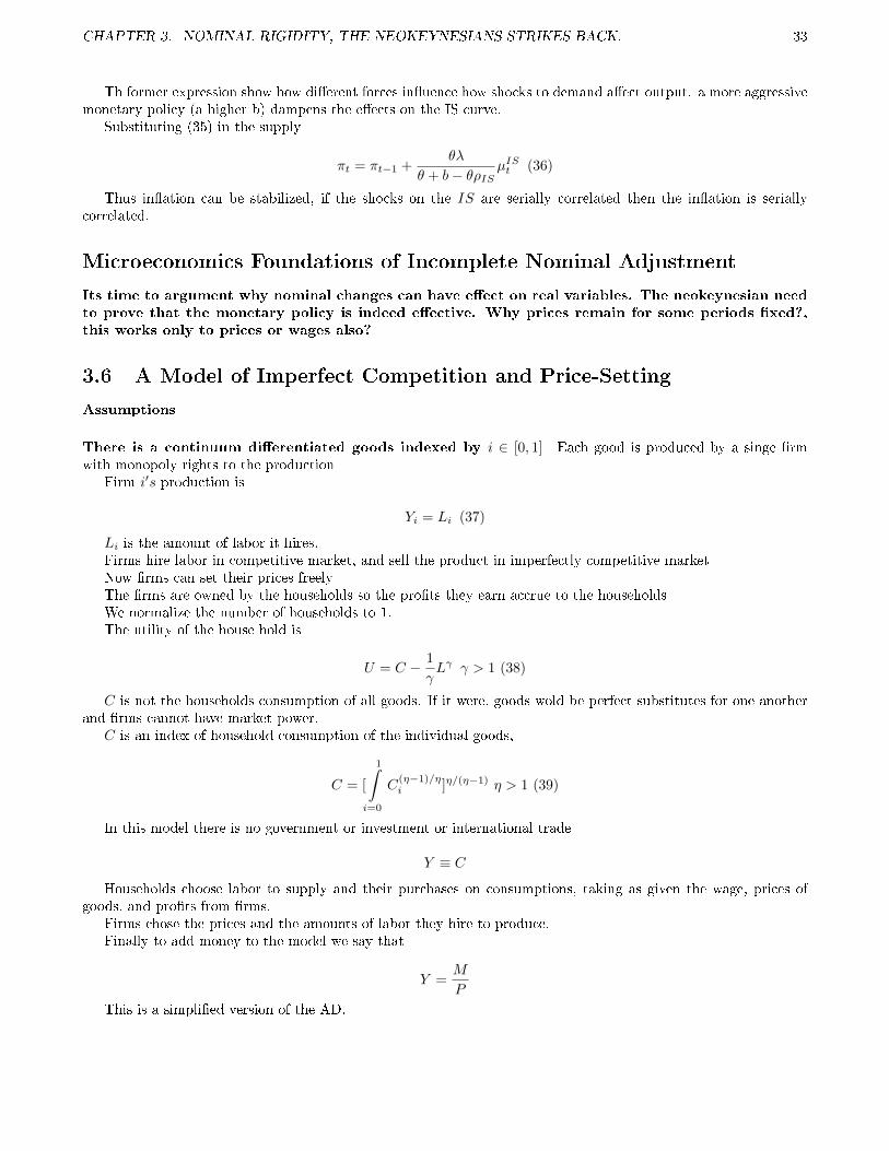
3.6 A Model of Imperfect Competition and Price-Setting
Assumptions
There is a continuum dierentiated goods indexed by i ∈ [0, 1] Each good is produced by a singe rmwith monopoly rights to the production
Firm i′s production is
Yi = Li (37)
Li is the amount of labor it hires.Firms hire labor in competitive market, and sell the product in imperfectly competitive marketNow rms can set their prices freelyThe rms are owned by the households so the prots they earn accrue to the householdsWe normalize the number of households to 1.The utility of the house hold is
U = C − 1
γLγ γ > 1 (38)
C is not the households consumption of all goods. If it were, goods wold be perfect substitutes for one anotherand rms cannot have market power.
C is an index of household consumption of the individual goods,
C = [
1ˆ
i=0
C(η−1)/ηi ]η/(η−1) η > 1 (39)
In this model there is no government or investment or international trade
Y ≡ C
Households choose labor to supply and their purchases on consumptions, taking as given the wage, prices ofgoods, and prots from rms.
Firms chose the prices and the amounts of labor they hire to produce.Finally to add money to the model we say that
Y =M
P
This is a simplied version of the AD.

CHAPTER 3. NOMINAL RIGIDITY, THE NEOKEYNESIANS STRIKES BACK. 34
3.6.1 The households behavior
Consider a household that expends SThen
L = [
1ˆ
i=0
C(η−1)/ηi ]η/(η−1)di+ λ[S −
1ˆ
i=0
CiPidi]
Then the rst order condition with respect Ci
η/(η − 1)[
1ˆ
j=0
C(η−1)/ηj ]1/(n−1)
η − 1
ηC−1/ηi = λPi
Note that the only therms that depend on i are Ci and Pi so it must be true that
Ci = AP−ηi
now subtitling in the budget constrain
S =
1ˆ
i=0
CiPidi
S =
1ˆ
j=0
AP 1−ηj dj
Solving for A
A =S´ 1
j=0P 1−ηj dj
Then
Ci =S´ 1
j=0P 1−ηj dj
P−ηi
And sustitutin in C
C = [
1ˆ
i=0
(S´ 1
j=0P 1−ηj dj
P−ηi
) η−1η
di]η/(η−1)
or
C =S´ 1
j=0P 1−ηj dj
[
1ˆ
i=0
(P−ηi
) η−1η di]η/(η−1)
C =S´ 1
j=0P 1−ηj dj
[
1ˆ
i=0
(P 1−ηi
)di]η/(η−1)
The last equation tell us that when households behave optimally, the cost of of obtaining one unit of C is´ 1i=0
(P 1−ηi
)di]η/(η−1) . That is the price index of the utility function
P =
1ˆ
i=0
(P 1−ηi
)di]1/(η−1)
Then
CHAPTER 3. NOMINAL RIGIDITY, THE NEOKEYNESIANS STRIKES BACK. 35
C =S´ 1
j=0P 1−ηj dj
P−η
Then Multiplying forP−ηiPI−η
C =S´ 1
j=0P 1−ηj dj
P−ηiPI−η
P−η
Ci =S´ 1
j=0P 1−ηj dj
P−ηi
C = CiP−η
P−ηi
Then
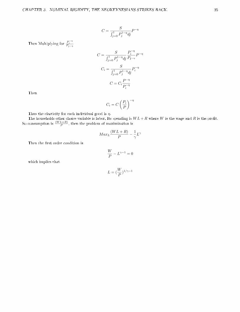
Ci = C
(PiP
)−ηThus the elasticity for each individual good is η.The households other choice variable is labor, Its spending is WL+R where W is the wage and R is the prot.
So consumption is (WL+R)P , then the problem of maximization is
MaxL(WL+R)
P− 1
γLγ
Then the rst order condition is
W
P− Lγ−1 = 0
which implies that
L = (W
P)1/γ−1