lectures in microeconomics-charles w. upton labor supply
Post on 21-Dec-2015
215 views
TRANSCRIPT
Lectures in Microeconomics-Charles W. Upton
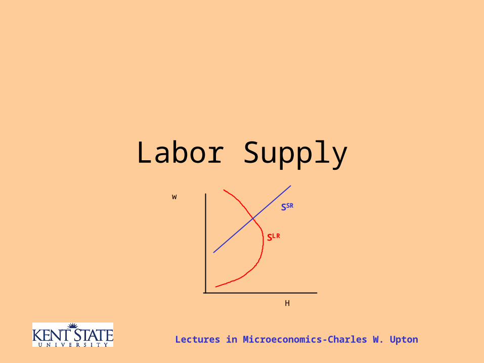
Labor Supplyw
H
SLR
SSR

Labor Supply
The Work Leisure Choice
X
I1
Io
H*
X=10H
X*

Labor Supply
The Work Leisure Choice
X
I1
Io
H*
X=10H
1680
168
X*

Labor Supply
The Work Leisure Choice
X
I1
Io
H*
X=10H
Io1680
168
X*

Labor Supply
The Work Leisure Choice
X
I1
Io
H*
X=10H
Io1680
168
X*
L*

Labor Supply
The Work Leisure Choice
X
I1
Io
H*
X=10H
Io1680
168
X*
L*
L*+H*=168

Labor Supply
The Backward Bending Labor Supply Curve
w
H
S

Labor Supply
The Backward Bending Labor Supply Curve
w
H
S•As wages initially rise, people work harder

Labor Supply
The Backward Bending Labor Supply Curve
w
H
S •At some point, people are making enough money and decide to work less.

Labor Supply
Hours worked over timeAverage Hours Worked Per Person
in the United States, 1870-1989
Year
Hours Worked
Per Capita
GDP (1989$)
Implied “Wage Rate”
1870 2,964 2,254 $0.76 1890 2,789 3,115 $1.12 1913 2,605 4,868 $1.87 1929 2,342 6,336 $2.71 1938 2,062 5,568 $2.70 1950 1,867 8,611 $4.61 1960 1,795 9,995 $5.57 1973 1,717 14,103 $8.21 1987 1,608 17,340 $10.78 1989 1,604 18,317 $11.42

Labor Supply
An Interpretation
• This is the long run labor supply curve.
Labor Supply
An Interpretation
• This is the long run labor supply curve.
• Normally, if an hour of leisure costs you more, you will purchase less of it
Labor Supply
An Interpretation
• This is the long run labor supply curve.
• Normally, if an hour of leisure costs you more, you will purchase less of it
• However, as your wage rate rises, your income rises and you want more leisure.

Labor Supply
An Interpretation
• Suppose your employer offered you an additional $10 an hour for every hour you worked this week and only this week.

Labor Supply
An Interpretation
• Suppose your employer offered you an additional $10 an hour for every hour you worked this week and only this week.
• You might decide to work 10 extra hours

Labor Supply
An Interpretation
• Suppose your employer offered you an additional $10 an hour for every hour you worked this week and only this week.
• You might decide to work 10 extra hours– There is a substitution effect.– The effect on your lifetime income is negligible

Labor Supply
An Interpretation
• Now suppose you got a permanent pay raise of $10 an hour.
Labor Supply
An Interpretation
• Now suppose you got a permanent pay raise of $10 an hour. – Most people would choose to work less over
their lifetime.

Labor Supply
An Interpretation
• Now suppose you got a permanent pay raise of $10 an hour. – Most people would choose to work less over
their lifetime.– They might not reduce the amount they work
right now, but might retire earlier.
Labor Supply
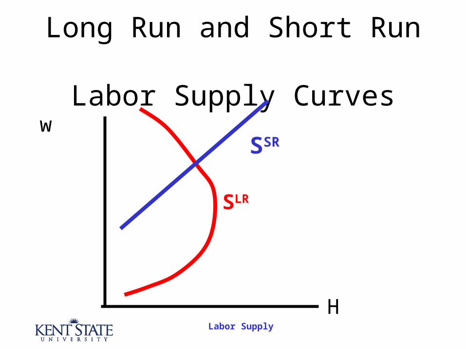
Long Run and Short Run Labor Supply Curves
w
H
SLR
SSR

Labor Supply
Long Run and Short Run Labor Supply Curves
w
H
SLR
SSR
The Long Run LS
Curve shows how people respond to a permanent
change in the wage rate.

Labor Supply
Long Run and Short Run Labor Supply Curves
w
H
SLR
SSR
The Short Run LS
Curve shows how people respond to a temporary
change in the wage rate.
Labor Supply
Some Examples
• College students work fewer hours than they would if this were their “permanent wage”.

Labor Supply
Some Examples
• College students work fewer hours than they would if this were their “permanent wage”.
• People who temporarily fall on hard times don’t work many hours at the low wages they can earn on a temporary job.

Labor Supply
Some Examples
• College students work fewer hours than they would if this were their “permanent wage”.
• People who temporarily fall on hard times don’t work many hours at the low wages they can earn on a temporary job.
• We all work hard when a lucrative opportunity comes along.

Labor Supply
Some Caveats
• The notion of a single week as a basis for labor supply is limiting

Labor Supply
Some Caveats
• The notion of a single week as a basis for labor supply is limiting.– Workers have traditionally varied their hours of
work over the course of the year. To adjust for the Christmas effect or the Finals week effect, we interpret this as an “average” week.

Labor Supply
Some Caveats
• The notion of a single week as a basis for labor supply is limiting.
• People “bunch” their labor supply at times when wage rates are higher when business is booming.

Labor Supply
Some Caveats
• The notion of a single week as a basis for labor supply is limiting.
• People “bunch” their labor supply at times when wage rates are higher when business is booming. Teachers work harder during
September - May

Labor Supply
Some Caveats
• The notion of a single week as a basis for labor supply is limiting.
• People “bunch” their labor supply at times when wage rates are higher when business is booming. Teachers work harder during
September - May
We all tend to work harder during the middle of our life span, for that is when the
combination of abilities and physical stamina is at its peak

Labor Supply
End
©2006 Charles W. Upton