lecture6 - the university of edinburgh · · 2016-06-28and faces a horizontal demand curve....
TRANSCRIPT
Competitive Firms and Markets
Lecture 6
Reading: Perlo¤ Chapter 8
August 2015
1 / 76

Introduction
We learned last lecture what input combination a �rm will use for agiven level of output.
But exactly how much should a �rm produce?
Depends on their cost structure, what other �rms will do and howconsumers behave.
2 / 76
Introduction
In this lecture, we see how the supply curve we saw on the �rst day isderived.
We look in more detail how the equilibrium quantity and price isdetermined in a perfectly competitive market.
3 / 76

Outline
Perfect Competition - A perfectly competitive �rm is a price takerand faces a horizontal demand curve.
Pro�t Maximization - How much should a �rm produce to maximizepro�ts?
Competition in the Short Run - What is the market equilibriumwhen the number of �rms in the market is �xed?
Competition in the Long Run - What is the market equilibriumwhen �rms are free to enter and exit?
4 / 76

Perfect Competition
One of the simplest market structures is perfect competition.A market is perfectly competitive if each �rm in the market is a pricetaker.A �rm is a price taker if it cannot alter the market price or the priceat which they buy inputs.
Everything the �rm needs to know is captured by the market price.
5 / 76

Perfect Competition
Firms are likely to be price takers if the market has some or all of theproperties
Huge number of �rmsHomogenous productsEverybody knows everythingLow transaction costsFree entry and exit
Obviously these conditions are never fully met, but many markets arehighly competitive.
6 / 76
Perfect Competition
Large Number of Buyers and Sellers
If there are enough sellers, no �rm can raise or lower the market price.
An individual �rm is a tiny percent of the entire market.
The �rm�s demand curve is a horizontal line at the market price.
7 / 76

Perfect Competition
Identical Products
Firms sell homogenous products.A good produced by �rm A is perfectly substitutable with a goodproduced by �rm B.
A �rm cannot sell anything if it raises its price by 1P more than itscompetitors.
An example of this would be Granny Smith apples or plain whitet-shirts.
8 / 76

Perfect Competition
Full Information
Buyers know the prices set by all �rms.
Firms cannot get away with raising their price because consumersknow the prices of all �rms.
9 / 76

Perfect Competition
Negligible Transaction Costs
Buyers and sellers don�t have to spend much time or money tointeract with each other.
If this were not the case, buyers might absorb a higher price chargedby �rms who have a lower transaction cost.
Think of all �rms as being in the same room.
10 / 76
Perfect Competition
Free Entry and Exit
If all �rms raise their prices and there is pro�t to be made, �rms willkeep entering until the price is driven back down.
If there were no free exit, �rms might be hesitant to enter the marketin case of a bad shock.
11 / 76
Perfect Competition
Many markets do not posses all these features, but are for practicalpurposes still price takers.
In these markets, �rms do not deviate signi�cantly from price taking.
We still call these markets competitive in practice.
12 / 76

Perfect Competition
The most important thing to take away from all this is that aperfectly competitive �rm faces a horizontal demand curve.
Lets see how this can occur.
13 / 76

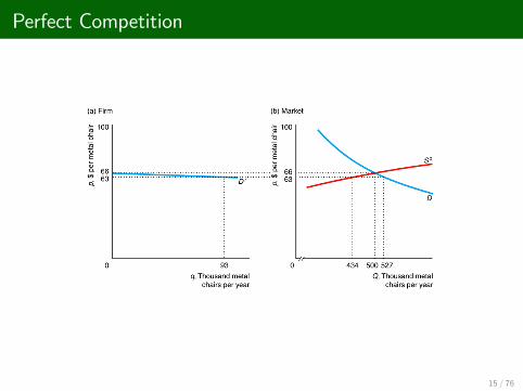
Perfect Competition
An individual �rm faces a residual demand curve.This is the market demand not met by other sellers.
It is equal to the market demand minus the supply of all other �rms.
D r (p) = D(p)� So (p)
For example, buyers want to purchase 10,000 bananas and all theother banana �rms sell 9,990 bananas. Residual demand is 10bananas.
14 / 76
Perfect Competition
15 / 76

Perfect Competition
Because the residual demand curve is much �atter than the marketdemand curve, the elasticity of residual demand is much higher thanmarket elasticity
If there are n identical �rms, the elasticity of demand facing �rm i is
εi = nε� (n� 1)ηo
εi is the elasticity facing �rm i . ε is the market elasticity and ηo isthe elasticity of supply of the other �rms
16 / 76
Perfect Competition
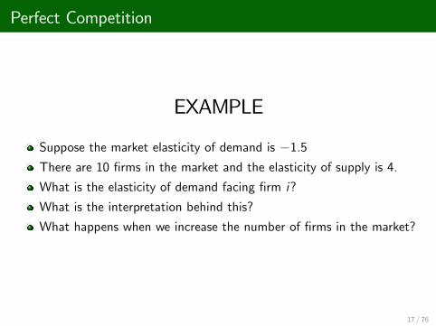
EXAMPLE
Suppose the market elasticity of demand is �1.5There are 10 �rms in the market and the elasticity of supply is 4.
What is the elasticity of demand facing �rm i?
What is the interpretation behind this?
What happens when we increase the number of �rms in the market?
17 / 76

Perfect Competition
As the number of �rms in the market increases, we approach aperfectly competitive market.
As we approach a perfectly competitive market, the demand curvefacing a single �rm gets �atter and �atter.
The key point is that an individual �rm is insigni�cant to whathappens in the market.
18 / 76
Perfect Competition
Why do we study perfect competition?
Many markets are reasonably described as competitive.Easy to model.Once we understand it, we can easily add imperfections to make itmore realistic.
19 / 76
Pro�t Maximization
To derive the market supply curve, we must know how much each�rm wants to produce.
We will �rst look at this in the short-run.
The �rm produces an amount such that its pro�ts are maximized.
Pro�t is just the di¤erence between total revenue and total costπ = TR � TC .Total revenue is the number of units you sell times the price of eachunit p � q.
20 / 76
Pro�t Maximization
Cost is a bit less straightforward.
We always refer to economic costs.Economic costs includes opportunity cost, accounting cost do not.
It might seem like your business is making money, but workingsomewhere else might be more pro�table.
21 / 76

Pro�t Maximization
There are two steps a �rm must make when �nding its pro�tmaximizing level of output.
The �rst step is the output decisionWhat level of output, q�, maximizes pro�t?
22 / 76
Pro�t Maximization
The next step is the shutdown decisionIs it more pro�table to produce q� or to shut down and producenothing?
23 / 76
Pro�t Maximization
A �rm can use any of the following three equivalent rules to choosehow much to produce.
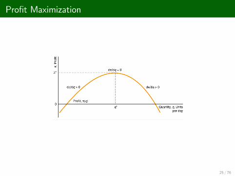
RULE 1 Maximize pro�t function
Find your pro�t function and �nd the maximum.
24 / 76
Pro�t Maximization
25 / 76

Pro�t Maximization
RULE 2 Set marginal pro�t to zero
Marginal pro�t is the extra pro�t you get from selling one more unit.
When marginal pro�t is zero, we will lose pro�t by increasing ordecreasing output (must check second order condition).
dπ(q)dq
= 0
26 / 76
Two Steps to Maximizing Pro�t-Step One
RULE 3 Set marginal revenue to equal to marginal cost
Marginal revenue is the additional revenue you get from increasingoutput.
Marginal cost is the addition cost you incur from increasing output.
At the optimum, MC (q) = MR(q).
27 / 76
Pro�t Maximization
These are all exactly the same thing
maxπ(q) = R(q)� C (q)dπ(q)dq
=dR(q)dq
� dC (q)dq
= 0
dR(q)dq
=dC (q)dq
28 / 76
Pro�t Maximization
EXAMPLE
Suppose the market price is p = 100.
Our cost function is
C (q) = 20q + 10q2
What is the pro�t maximizing level of output?
29 / 76
Pro�t Maximization
After you know what q� is, all we have to know whether or not weshould shut down.
Remember that in the short run, we can have sunk �xed costs.If a �rm shuts down in the short run, it still has to pay sunk �xedcosts.
A �rm might stay in business if it is making a loss if it is covering itssunk �xed costs.
30 / 76
Pro�t Maximization
The sunk cost should not play a role in the �rm�s shut down decision.
The �rm only needs to make sure its costs are less than the avoidablecosts.
31 / 76
Pro�t Maximization
Suppose
Total Revenue = 5000
Variable Cost = 2000
Sunk Fixed Cost = 6000
Should the �rm shut down?
32 / 76
Pro�t Maximization
We just need to compare the pro�t from staying in business versusnot (πO is pro�t from staying in business and πSD is pro�t fromshutting down).
πO = 5000� 2000� 6000 = �3000πSD = �6000
The �rm minimizes its losses by staying in business
33 / 76
Competition in the Short Run
Okay, we know how much an individual �rm decides its productionlevel.
We can use this information to �nd out what total market productionand the market price is.
First, we need to �nd the supply curve of each individual �rm.
34 / 76
Competition in the Short Run
REMEMBER, �rms in competitive markets face a horizontal demandcurve.
No matter how much an individual �rm sells, the price will notchange.
The price they get from each unit is constant ) R(q) = p � q.The market price is independent of how much an individual �rmproduces.
35 / 76

Competition in the Short Run
Because the price is the same no matter how much one �rmproduces, marginal revenue is simply MR(q) = dR (q)
dq = p.
The pro�t maximizing level of output occurs where MR(q) = MC (q)
Therefore the pro�t maximizing level of output occurs where
MC (q) = p
36 / 76

Competition in the Short Run
The �rm�s supply curve is the marginal cost curve above theshut-down price.
That is, the �rm sees the market price and decides how much toproduce according to its marginal cost curve.
37 / 76
Competition in the Short Run
EXAMPLE
Suppose the shutdown price for a �rm is p = 0.
What is the �rms supply curve if the cost function is
C (q) = 2q2 + q + 12
38 / 76

Competition in the Short Run
How do we �nd the shut-down price?
At q�, we can �nd the �rm�s average pro�t as follows
π
q=Rq� Cq=pqq� Cq= p � AC
For example, If the price is $10 and the average cost of producingeach unit is $3, your average pro�t is $7.
39 / 76

Competition in the Short Run
40 / 76
Competition in the Short Run
Remember �rms in the short run only care about covering theirvariable costs.
The �rm can only gain from shutting down if its revenue is less thanits short-run variable cost pq < VC (q)
Divide both sides by q to show the �rm shuts down if the market priceis less than the minimum of its short-run average variable cost curve
p <VC (q)q
= AVC
41 / 76

Competition in the Short Run
42 / 76

Competition in the Short Run
We know that �rms will shut down if price is p < AVC
We also know that to maximize pro�t the �rm will produce wherep = MC (q)
The �rm will shutdown when MC < AVC
This occurs at the minimum of the average variable cost curve) The �rm�s shut down price in the short-run is the minimum of theaverage variable cost curve.
43 / 76

Competition in the Short Run
There are two ways we can �nd the shut-down price in the short-run.
1 Minimize the AVC function and �nd the corresponding price.2 Find the price where AVC = MC
44 / 76

Competition in the Short Run
The supply curve is just the marginal cost curve above the minimumof the average cost curve
S(p) =�MC (q) if p � pshutdown0 if p < pshutdown
45 / 76

Competition in the Short Run
46 / 76
Competition in the Short Run
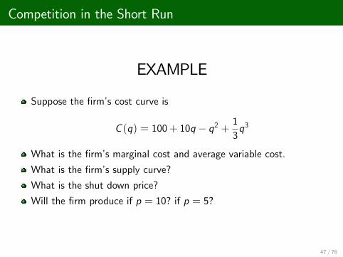
EXAMPLE
Suppose the �rm�s cost curve is
C (q) = 100+ 10q � q2 + 13q3
What is the �rm�s marginal cost and average variable cost.
What is the �rm�s supply curve?
What is the shut down price?
Will the �rm produce if p = 10? if p = 5?
47 / 76
Competition in the Short Run
We saw how to get one �rm�s supply curve
The market supply curve is the horizontal sum of all the �rm�s in themarkets supply curve
In the short run, the number of �rms is �xed at n
48 / 76
Competition in the Short Run
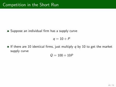
Suppose an individual �rm has a supply curve
q = 10+ P
If there are 10 identical �rms, just multiply q by 10 to get the marketsupply curve
Q = 100+ 10P
49 / 76

Competition in the Short Run
The more �rms we have, the �atter is the market supply curve
50 / 76
Competition in the Short Run
If �rms di¤er, the marginal cost curves will not be identical.
The shut down prices of �rms will not be the same either.
51 / 76

Competition in the Short Run
52 / 76

Competition in the Short Run
By combining the short-run market supply curve and the marketdemand curve, we can �nd the short-run equilibrium
53 / 76

Competition in the Short Run
In summary...
Each �rm will produce the level of output where MC = p.
We add up the individual �rm supply curves to get the market supplycurve.
The market price is determined by the intersection of the marketsupply curve and the market demand curve.
54 / 76
Competition in the Short Run
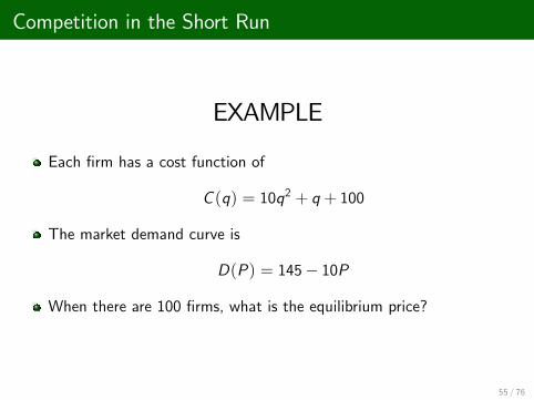
EXAMPLE
Each �rm has a cost function of
C (q) = 10q2 + q + 100
The market demand curve is
D(P) = 145� 10P
When there are 100 �rms, what is the equilibrium price?
55 / 76
Competition in the Long Run
There are two key di¤erences in between the short and long run
1 There are no sunk �xed costs2 The number of �rms in the market is not �xed
56 / 76

Competition in the Long Run
How much will each �rm produce in the long-run?
Once again, �rms select the level of output which maximizes theirpro�t.
The pro�t maximizing level of output occurs where p = MC .
57 / 76
Competition in the Long Run
After determining the pro�t maximizing level of output q�, the �rmmust decide whether or not to shutdown.
In the long run, all costs are variable.
Unlike in the short-run, the �rm will shut down if it incurs any lossesat all.
The �rm will shut down when p < AC .
The shut-down price occurs at the minimum of the average costcurve.
58 / 76
Competition in the Long Run
There are two ways we can �nd the shut-down price in the long-run.
1 Minimize the AC function and �nd the corresponding price.2 Find the price where AC = MC
59 / 76
Competition in the Long Run
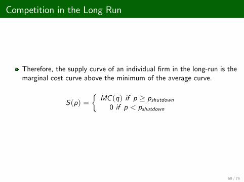
Therefore, the supply curve of an individual �rm in the long-run is themarginal cost curve above the minimum of the average curve.
S(p) =�MC (q) if p � pshutdown0 if p < pshutdown
60 / 76

Competition in the Long Run
EXAMPLE
What is the supply curve for a �rm in the long-run with the costfunction:
C (q) = 40q � q2 + .01q3
61 / 76
Competition in the Long Run
The market supply curve is once again the horizontal sum of all �rms�supply curves.
In the short-run, the number of �rms is �xed, but �rms can enter orleave the market in the long run.
62 / 76

Competition in the Long Run
If there are pro�ts to be made, �rms will enter the market as there areno barriers in perfect competition.
This will cause the market supply curve to shift and the market priceto fall.
If there is negative pro�t, �rms will exit.
The number of �rms is determined by π = 0.
63 / 76
Competition in the Long Run
Firms make zero pro�t when p = pSD where pSD is the shutdownprice.
The shutdown price occurs at the minimum of the average cost curve.
Therefore, the market price will always occur at the minimum of theaverage cost curve.
64 / 76
Competition in the Long Run
EXAMPLE
Draw the market supply and demand curves in one graph next to agraph showing an individual �rms�s average/marginal cost curves.
Identify two market prices, p1 and p2. At price p1, �rms will enterthe market and at price p2, �rms will exit the market.
65 / 76
Competition in the Long Run
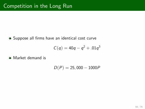
Suppose all �rms have an identical cost curve
C (q) = 40q � q2 + .01q3
Market demand is
D(P) = 25, 000� 1000P
66 / 76

Competition in the Long Run
We have three equilibrium conditions in the long run. P� is themarket price and n� is the number of �rms.
1 Pro�t Maximization
P� = MC ! P� = 40� 2q + .03q2
2 Zero Pro�tP� = AC ! P� = 40� q + .01q2
3 Supply equals demand
nq = 25, 000� 1000P
67 / 76
Competition in the Long Run
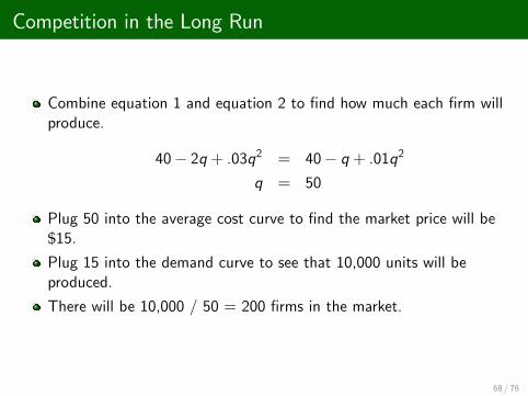
Combine equation 1 and equation 2 to �nd how much each �rm willproduce.
40� 2q + .03q2 = 40� q + .01q2
q = 50
Plug 50 into the average cost curve to �nd the market price will be$15.Plug 15 into the demand curve to see that 10,000 units will beproduced.
There will be 10,000 / 50 = 200 �rms in the market.
68 / 76
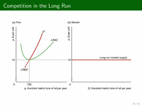
Competition in the Long Run
The long run market supply curve is �at at the minimum long runaverage cost curve i¤
input prices are constant.�rms have identical costs.
69 / 76
Competition in the Long Run
70 / 76

Competition in the Long Run
Remember how we said there is no such thing as the law of supply?
The supply curve can slope upwards or downwards if the previous twoconditions are not met.
71 / 76
Competition in the Long Run
If entry is limited, the market supply curve will slop upward.
Individual �rms have upward sloping supply curves.The only way to increase output is for existing �rms to produce more.
72 / 76

Competition in the Long Run
If �rms di¤er in their costs, the market supply curve will also slopeupwards.
Some �rms will enter the market at lower prices than others.
73 / 76
Competition in the Long Run
If the number of co¤ee shops increases, we could expect the price ofco¤ee beans to increase.
This will also cause the market supply curve to be upward sloping.
It is also possible for input prices to decrease with output (economiesof scale).
This will cause the supply curve to be downward sloping.
74 / 76
Summary
What are the conditions under which �rms are price takers?
What is the residual demand curve?
The �rm will shut down so long as the price is greater than what?
The supply curve is the _____ above _____.
75 / 76

Summary
How do you determine the market price in the long-run?
How do you determine the number of �rms in the long-run?
When will the long-run market supply curve slope upwards?
When will the long-run market supply curve slope upwards?
76 / 76