lecture6 positive definite matrices - national chiao tung...

Linear Algebra

Lecture 6PositiveDefiniteMatrices

Prof. Chun-Hung Liu

2017/6/8 Lecture6:PositiveDefiniteMatrices 1

Dept. of Electrical and Computer EngineeringNational Chiao Tung University

Spring 2017


Outline

• Minima, Maxima, and Saddle Points

• Tests for Positive Definiteness

• Singular Value Decomposition

(The materials of this lecture are based on Chapter 6 of Strang’s Book)


Minima, Maxima, and Saddle Points• The signs of the eigenvalues are often crucial. For stability in differential

equations, we needed negative eigenvalues so that would decay.e�t

• The new and highly important problem is to recognize a minimum point.Here are two examples:

Does either or have a minimum at the point ?F (x, y) f(x, y) x = y = 0

Remark 1. The zero-order terms and have no effect on the answer. They simply raise or lower the graphs of F and f .

F (0, 0) = 7 f(0, 0) = 0

Remark 2. The linear terms give a necessary condition: To have any chance of a minimum, the first derivatives must vanish at :x = y = 0


Thus is a stationary point for both functions.

Remark 3. The second derivatives at (0,0) are decisive:

These second derivatives 4, 4, 2 contain the answer. Since they are the same for F and f, they must contain the same answer. F has a minimum if and only if f has a minimum.

Minima, Maxima, and Saddle Points

(x, y) = (0, 0)


Minima, Maxima, and Saddle PointsRemark 4. The higher-degree terms in F have no effect on the question of a local minimum, but they can prevent it from being a global minimum.

• Every quadratic form has a stationary point at the origin, where . A local minimum would also be a global minimum, the surface will then be shaped like a bowl, resting on the origin (Figure 6.1).

f = ax

2 + 2bxy + cy

2

@f/@x = @f/@y = 0z = f(x, y)


Minima, Maxima, and Saddle Points• If the stationary point of F is at , the only change would

be to use the second derivatives at :x = ↵, y = �

↵,�

This behaves near (0,0) in the same way that behaves near .

f(x, y)F (x, y)

(↵,�)

• The third derivatives are drawn into the problem when the second derivatives fail to give a definite decision. That happens when the quadratic part is singular.

• For a true minimum, f is allowed to vanish only at . When is strictly positive at all other points (the bowl goes up), it is called

positive definite.

x = y = 0f(x, y)


Minima, Maxima, and Saddle Points• Definite versus Indefinite: Bowl versus Saddle

What conditions on a, b, and c ensure that the quadratic is positive definite? One necessary condition

is easy:f(x, y) = ax

2 + 2bxy + cy

2

(i) If is positive definite, then necessarily .ax

2 + 2bxy + cy

2 a > 0

(ii) If is positive definite, then necessarily .f(x, y) c > 0


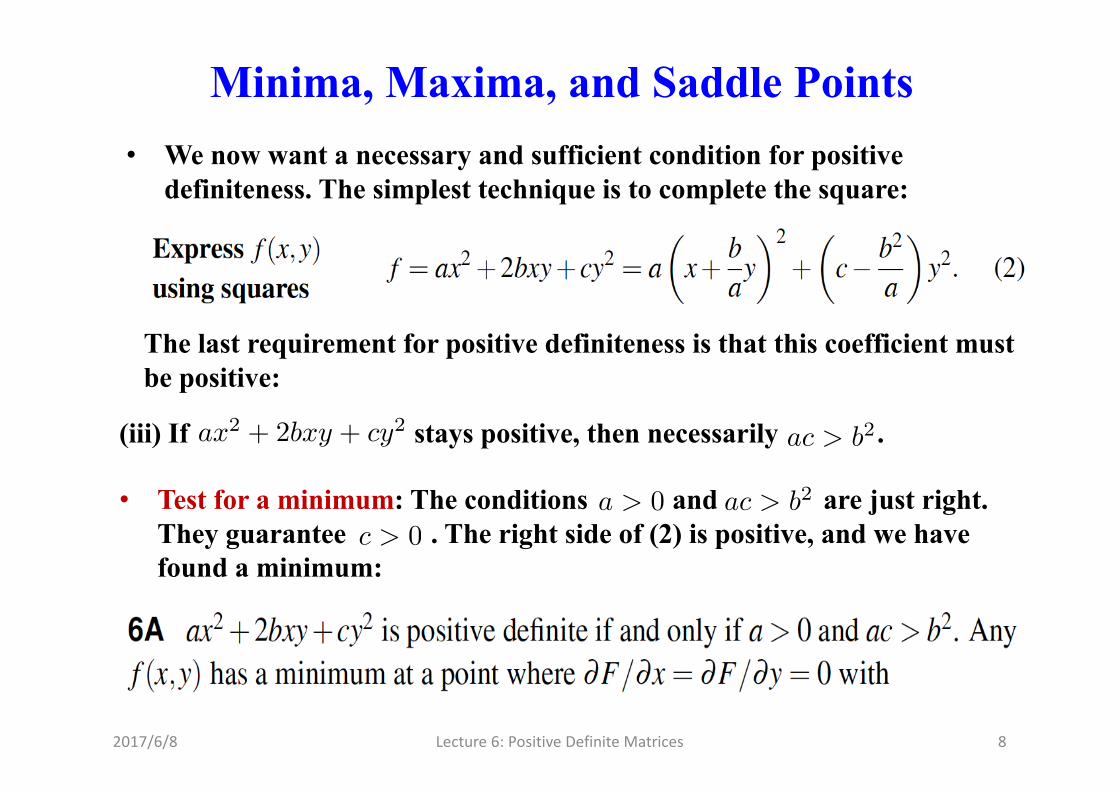
Minima, Maxima, and Saddle Points• We now want a necessary and sufficient condition for positive

definiteness. The simplest technique is to complete the square:

The last requirement for positive definiteness is that this coefficient must be positive:

(iii) If stays positive, then necessarily .ax

2 + 2bxy + cy

2 ac > b2

• Test for a minimum: The conditions and are just right. They guarantee . The right side of (2) is positive, and we have found a minimum:

a > 0 ac > b2

c > 0



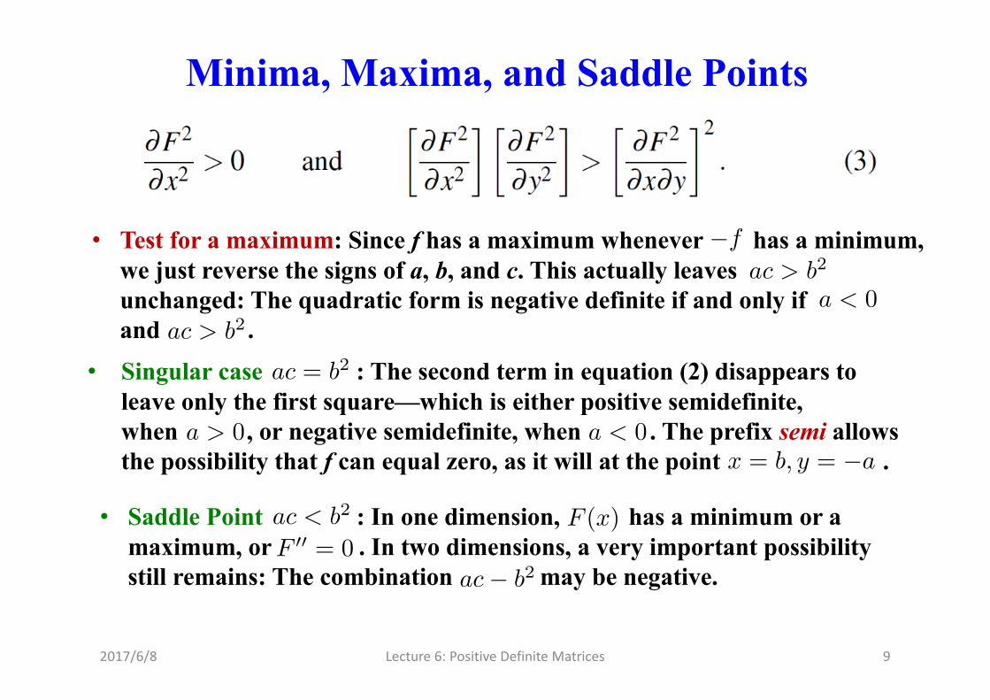
• Test for a maximum: Since f has a maximum whenever has a minimum, we just reverse the signs of a, b, and c. This actually leaves unchanged: The quadratic form is negative definite if and only if and .

ac > b2

a < 0ac > b2

�f

• Singular case : The second term in equation (2) disappears to leave only the first square—which is either positive semidefinite, when , or negative semidefinite, when . The prefix semi allows the possibility that f can equal zero, as it will at the point .

ac = b2

a > 0 a < 0x = b, y = �a

• Saddle Point : In one dimension, has a minimum or a maximum, or . In two dimensions, a very important possibility still remains: The combination may be negative.

ac < b2

F 00 = 0F (x)

ac� b2


Minima, Maxima, and Saddle Points• It is useful to consider two special cases:

In the first, b=1 dominates a=c=0. In the second, a=1 and c=-1 have opposite sign. The saddles and are practically the same.2xy x

2 � y

2

• These quadratic forms are indefinite, because they can take either sign. So we have a stationary point that is neither a maximum or a minimum. It is called a saddle point.

• Higher Dimensions: Linear Algebra

A quadratic comes directly from a symmetric 2 by 2 matrix:f(x, y)



• For any symmetric matrix A, the product is a pure quadratic form :

x

TAx

f(x1, . . . , xn)

The function is zero at , and its first derivatives are zero. The tangent is flat; this is a stationary point. We have to decide if is a minimum or a maximum or a saddle point of the function .

x = (0, . . . , 0)x = 0

f = x

TAx



• At a stationary point all first derivatives are zero. • A is the “second derivative matrix” with entries .

This automatically equals , so A is symmetric. • Then F has a minimum when the pure quadratic is positive

definite. These second-order terms control F near the stationary point:

aij = @

2F/@xi@xj

aji = @

2F/@xj@xi

x

TAx

At a stationary point, grad is a vector of zeros.

F = (@F/@x1, . . . , @F/@xn)


Tests for Positive Definiteness• Which symmetric matrices have the property that for all

nonzero vectors x? The previous section began with some hints about the signs of eigenvalues. But that gave place to the tests on a, b, c:

x

TAx > 0

From those conditions, both eigenvalues are positive. Their product is determinant , so the eigenvalues are either both positive or both negative. They must be positive because their sum is the trace .

�1�2

ac� b2 > 0a+ c > 0

• Looking at a and , it is even possible to spot the appearance of the pivots:

ac� b2

Those coefficients a and are the pivots for a 2 by 2 matrix.(ac� b2)/a

A=


Tests for Positive Definiteness• For larger matrices the pivots still give a simple test for positive

definiteness: stays positive when n independent squares are multiplied by positive pivots.

x

TAx

• The natural generalization will involve all n of the upper left submatrices of A:

• Here is the main theorem on positive definiteness


Tests for Positive DefinitenessProof. Condition I defines a positive definite matrix. Our first step shows that each eigenvalue will be positive:

A positive definite matrix has positive eigenvalues, since .x

TAx > 0

If all , we have to prove for every vector x (not just the eigenvectors). Since symmetric matrices have a full set of orthonormal eigenvectors, any x is a combination . Then

�i > 0x

TAx > 0

c1x1 + · · ·+ cnxn

Because of the orthogonality , and the normalization ,x

Ti xj = 0 x

Ti xi = 0

If every , then equation (2) shows that . Thus condition II implies condition I.

x

TAx > 0�i > 0


Tests for Positive DefinitenessIf condition I holds, so does condition III: The determinant of A is the product of the eigenvalues. The trick is to look at all nonzero vectors whose last n-k components are zero:

Thus is positive definite. Its eigenvalues must be positive. Its determinant is their product, so all upper left determinants are positive.

Ak

If condition III holds, so does condition IV: If the determinants are all positive, so are the pivots.

If condition IV holds, so does condition I: We are given positive pivots, and must deduce that .

x

TAx > 0


Those positive pivots in D multiply perfect squares to make positive. Thus condition IV implies condition I.

x

TAx

Tests for Positive Definiteness


Tests for Positive Definiteness• Positive Definite Matrices and Least Squares: The rectangular matrix

will be R and the least-squares problem will be . It has mequations with (square systems are included). The least-square choice is the solution of .

Rx = b

m � nbx R

TRbx = R

Tb

• That matrix is not only symmetric but positive definite provided that the n columns of R are linearly independent:

The key is to recognize as . This squared length is positive (unless x = 0), because R has independent columns. (If x is nonzero then Rx is nonzero.). Thus and is positive definite.

x

TAx x

TR

TRx = (Rx)T (Rx)

kRxk2x

TR

TRx > 0 RTR

A = RTR


Tests for Positive Definiteness• It remains to find an R for which .A = RTR

This Cholesky decomposition has the pivots split evenly between L and .LT

A third possibility is , the symmetric positive definite square root of A.

R = Qp⇤QT


Tests for Positive Definiteness• Semidefinite Matrices:

The diagonalization leads to . If Ahas rank r, there are r nonzero ’s and r perfect squares in

A = Q⇤QTx

TAx = x

TQ⇤QT

x = y

T⇤y�

yT⇤y = �1y21 + · · ·+ �ry2r


Tests for Positive Definiteness• Ellipsoids in n Dimensions

The equation to consider is . If A is the identity matrix, this simplifies to . This is the equation of the “unit sphere” in . If , the sphere gets smaller. The equation changes to .

x

TAx = 1

x

21 + x

22 + · · ·+ x

2n = 1

Rn A = 4I4x2

1 + · · ·+ 4x2n = 1

• The important step is to go from the identity matrix to a diagonal matrix:



• To locate the ellipse we compute and . The unit eigenvectors are and .

�1 = 1 �2 = 9(1,�1)/

p2 (1, 1)/

p2


• The way to see the ellipse properly is to rewrite :x

TAx = 1

Note and are outside the squares. The eigenvectors are inside.� = 1 � = 9

• Any ellipsoid can be simplified in the same way. The key step is to diagonalize . Algebraically, the change to produces a sum of squares:

x

TAx = 1A = Q⇤QT

y = Q

Tx

The major axis has along the eigenvector with the smallest eigenvalue. The other axes are along the other eigenvectors. Their lengths are .

y1 = 1/p�1

1/p�2, . . . , 1/

p�n



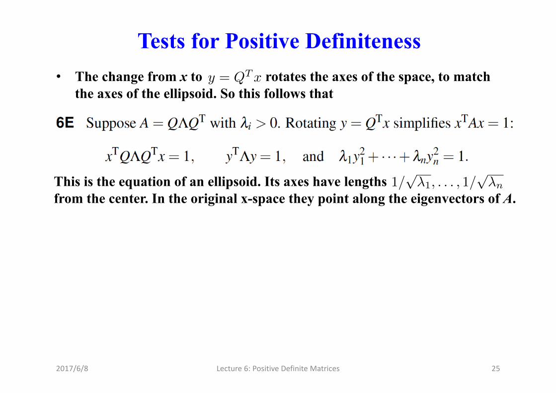
Tests for Positive Definiteness• The change from x to rotates the axes of the space, to match

the axes of the ellipsoid. So this follows thaty = Q

Tx

This is the equation of an ellipsoid. Its axes have lengths from the center. In the original x-space they point along the eigenvectors of A.

1/p�1, . . . , 1/

p�n


• The Generalized Eigenvalue Problem: For some engineering problems, sometimes is replaced by . There are two matrices rather than one.


Ax = �x

Ax = �Mx

• An example is the motion of two unequal masses in a line of springs:

When the masses were equal, , this was the old system . Now it is , with a mass matrix M.

m1 = m2 = 1u00 +Au = 0 Mu00 +Au = 0

• The eigenvalue problem arises when we look for exponential solutions:

e

i!tx



We work out with and :det(A� �M) m1 = 1 m2 = 2

• The underlying theory is easier to explain if M is split into . (M is assumed to be positive definite.) Then the substitution changes

RTRy = Rx

Writing C for , and multiplying through by , this becomes a standard eigenvalue problem for the single symmetric matrix :

R�1 (RT )�1 = CT

CTAC



• The properties of lead directly to the properties of , when and M is positive definite:

CTAC Ax = �Mx

A = AT

A and M are being simultaneously diagonalized. If S has the in its columns, then and .

xj

STAS = ⇤ STMS = I

• The main point is easy to summarize: As long as M is positive definite, the generalized eigenvalue problem behaves exactly like .

Ax = ��Mx Ax = �x


Singular Value Decomposition (SVD)• The SVD is closely associated with the eigenvalue-eigenvector

factorization of a positive definite matrix.• But now we allow the Q on the left and the on the right to be any two

orthogonal matrices U and —not necessarily transposes of each other. Then every matrix will split into .

• The diagonal (but rectangular) matrix has eigenvalues from , not from A! Those positive entries (also called sigma) will be

. They are the singular values of A. They fill the first rplaces on the main diagonal of —when A has rank r. The rest of is zero.

Q⇤QT

QT

V T

A = U⌃V T

⌃ ATA

�1, . . . ,�r

⌃ ⌃

• Singular Value Decomposition: Any m by n matrix A can be factored into


Singular Value Decomposition


• Application of the SVD: The SVD is terrific for numerically stable computations. because U and V are orthogonal matrices. They never change the length of a vector. Since , multiplication by U cannot destroy the scaling.


kUxk2 = x

TU

TUx = kxk2

• Image processing: Suppose a satellite takes a picture, and wants to send it to Earth. The picture may contain 1000 by 1000 “pixels”—a million little squares, each with a definite color. We can code the colors, and send back 1,000,000 numbers. It is better to find the essential information inside the 1000 by 1000 matrix, and send only that.• Suppose we know the SVD. The key is in the singular values (in ).

Typically, ’s are significant and others are extremely small. If we keep 20 and throw away 980, then we send only the corresponding 20 columns of U and V.

• We can do the matrix multiplication as columns times rows:

⌃�

Any matrix is the sum of r matrices of rank 1. If only 20 terms are kept, we send 20 times 2000 numbers instead of a million.


Singular Value Decomposition• The effective rank: The rank of a matrix is the number of independent

rows, and the number of independent columns. Consider the following:

The first has rank 1, although roundoff error will probably produce a second pivot. Both pivots will be small; how many do we ignore? The second has one small pivot, but we cannot pretend that its row is insignificant. The third has two pivots and its rank is 2, but its “effective rank” ought to be 1.

We go to a more stable measure of rank. The first step is to use or , which are symmetric but share the same rank as A. Their eigenvalues—the singular values squared—are not misleading. Based on the accuracy of the data, we decide on a tolerance like and count the singular values above it—that is the effective rank.

10�6

AAT ATA


• Polar decomposition: Every nonzero complex number z is a positive number r times a number on the unit circle: . The SVD extends this “polar factorization” to matrices of any size:


ei✓ z = rei✓

For proof we just insert into the middle of the SVD:V TV = I

The factor is symmetric and semidefinite (because is). The factor is an orthogonal matrix (because ).

S = V ⌃V T ⌃Q = UV T QQT = V UTUV T = I



• Least Squares: For a rectangular system , the least-squares solution comes from the normal equations . If A has dependent columns then is not invertible and is not determined.

• We have to choose a particular solution of , and we choose the shortest.

Ax = b

A

TAbx = A

Tb

ATA bxA

TAbx = A

Tb


Singular Value Decomposition• That minimum length solution will be called .

x

+



Based on this example, we know and for any diagonal matrix :⌃+x

+ ⌃

• Now we find in the general case. We claim that the shortest solution is always in the row space of A. Remember that any vector can be split into a row space component and a nullspace component:

x

+x

+

bxxr bx = xr + xn


• There are three important points about that splitting:


The fundamental theorem of linear algebra was in Figure 3.4. Every p in the column space comes from one and only one vector in the row space. All we are doing is to choose that vector, , as the best solution to .

xr

x

+ = xr

Ax = b



• The row space of A is the column space of . Here is a formula for :A+ A+

Proof. Multiplication by the orthogonal matrix leaves lengths unchanged:UT

Introduce the new unknown , which has the same length as x. Then, minimizing is the same as minimizing . Now is diagonal and we know the best . It is so the best is :

y = V

Tx = V

�1x

kAx� bk k⌃y � UT bk⌃ y+ y+ = ⌃+UT bx

+ V y+

is in the row space, and from the SVD.V y+ A

TAx

+ = A

Tb

+


Minimum Principles• Our goal here is to find the minimum principle that is equivalent

to , and the minimization equivalent to .Ax = b

Ax = �b

• The first step is straightforward: We want to find the “parabola” whose minimum occurs when . If A is just a scalar, that is easy to do:

P (x)Ax = b

This point will be a minimum if A is positive. Then the parabola opens upward (Figure 6.4).

x = A

�1b

P (x)

Proof. Suppose . For any vector y, we show that :Ax = b

P (y) � P (x)


Minimum Principles


Minimum Principles

This can’t be negative since A is positive definite—and it is zero only if . At all other points is larger than , so the minimum occurs at x.y � x = 0 P (y)

P (x)


Minimum Principles• Minimizing with Constraints: Many applications add extra equations

on top of the minimization problem. These equations are constraints. We minimize subject to the extra requirement .Cx = d

Cx = d

• Usually x can’t satisfy n equations and also extra constraints . So we need more unknowns.

Ax = b `Cx = d `

• Those new unknowns are called Lagrange multipliers. They build the constraint into a function . Thus, we can have

y1, . . . , y`L(x, y)

P (x)

When we set the derivatives of L to zero, we have equations for unknowns x and y:

n+ `n+ `


Minimum Principles


Minimum Principles

• Figure 6.5 shows what problem the linear algebra has solved, if the constraint keeps x on a line . We are looking for the closest point to (0,0) on this line. The solution is .

2x1 � x2 = 5x = (2,�1)

• Least Squares Again: The best is the vector that minimizes the squared error , i.e.,

bxE

2 = kAx� bk2

Compare with at the start of the section, which led to :12x

TAx� x

Tb

Ax = b


Minimum Principles

• The minimizing equation changes into theAx = b


Matrix Factorizations



12.

lecture6 positive definite matrices - national chiao tung...

Documents