Lecture 2

Signals and Systems,Discrete Convolutions

Signals and Systems

mappingInputF

outputGSystem :

ContinuousAnalog System :

elements of F and G are functions of continuous variables

Discretedigital System :

elements of F and G are sequences of numbers

Notation :

f[n] : a sequence of numbers, real or complex, defined for every integer n (discrete time index).

2

Ex. 1 : f[n] : real

-2-1

0 1 2 3

If f[n] is complex, then phase sequence must be defined

Ex. 2 : δ Sequence : position indicator (Unit Impulse)

δ[n] =

δ[n-k] = knkn

=≠

,1,0{

0,10,0{ =

≠nn

∑∞

−∞=

=k

kfnf k]-[n][][ δ ….(1)

weighted sum of delta sequences

-1 0 1 2 3

1 δ[n-1]

-1 0 1 2 3

1 δ[n]

3

Sampling Process :

)(][ tfnf s≡

∑∞

−∞=

−•=k

kttf )()( δ ….(2)

A discrete system is a rule for assigning to a sequence f[n] another sequence g[n] and denoted it as

g[n] = L{f[n]}

f[n] L g[n] = L{f[n]}input output

Impulse train

4

Characteristics of L

• Linear v.s. Non-linear• With Memory v.s. Memoryless• Time-invariant v.s. Time Varying• Feed forward v.s. Feedback• Stable v.s. Non-stable• Causal v.s. Non-Causal• Deterministic v.s. random

5

Ex. 3 :

(a) ][][ 2 nfng =• non-linear system• g[n] depends only on f[n](memoryless system)

(b) ][][ nnfng =• linear• memoryless• time-varying

(c) ]1[3][2][ −+= nfnfng• this system has finite memory• linear

(d) ][]1[2][ nfngng =−+• g[n] depends on both f[n] and g[n-1]

g[n] is obtained by solving a recursive equation

System with feedback; stability

problem

¤ Under certain condition (Causality), these equations have a unique solution. Initial condition 6

Basic Operations(i) Delay Element : g[n] = f[n-1]

1−zf[n] g[n] = f[n-1]

(ii)Multiplier : g[n] = a f[n]

gaina

f[n] g[n] = a f[n]

(iii)Adder : g[n] = ][][ 21 nfnf +

Any arbitrary LTI system can be realized by a combination of delay elements, multipliers and adders

⊕ ][][][ 21 nfnf ng +=][1 nf

][2 nf

7

Ex. 4 :

(i) g[n] = 2 f[n] + 3 f[n-1]

2

1−z3

⊕

f[n] f[n-1]

g[n]

(ii)g[n] + 2 g[n-1] = f[n]

1−z

-2

⊕f[n] g[n]

g[n-1]8

System Properties:- Linearity: L{ a1f1[n] + a2f2[n] }

= a1L{f1[n]} + a2L{f2[n]}- Time-Invariance: L{f[n-k]} = g[n-k] , for all k

where L{f[n]} = g[n]※ Linear and Time-Invariant system = LTI-system

※ Impulse Response (delta response)h[n] L{δ[n]}- Causality

If h[n] = 0 for n < 0 , causal system

Ex.(a) g[n] = f[n] + 1/2f[n-1] + … + (1/2)kf[n-k] + …h[n] =δ[n] + 1/2δ[n-1] + … +(1/2)kδ[n-k] + …

= (1/2)n , n≧0 - discrete exponential sequence 0 , n<0 - causal

- infinite delays(infinite-order system)

9

Ex.(b) g[n] – 1/2g[n-1] = f[n] ,with causality assumptionh[n] – 1/2h[n-1] =δ[n] ,for all n≧0 - one delaysetting n = 0,1,… and noting that h[n-1] = 0

h[n] = (1/2)n , n≧0 0 , n<0

(a),(b) are equivalent(same response to the same input) : Horner’s rule

1−z

1/2

⊕f[n] g[n]

g[n-1]

10

Discrete Convolutions(Digital Convolutions)

n)convolutio(linear h[n]*f[n]

)definition(by k]-f[k]h[n

)(linearity k]}-nf[k]L{δ[

)definition(by }k]-nf[k]δ[L{

L{f[n]} g[n]

-k

-k

-k

≡

=

=

=

=

∑

∑

∑

∞

∞=

∞

∞=

∞

∞=

11

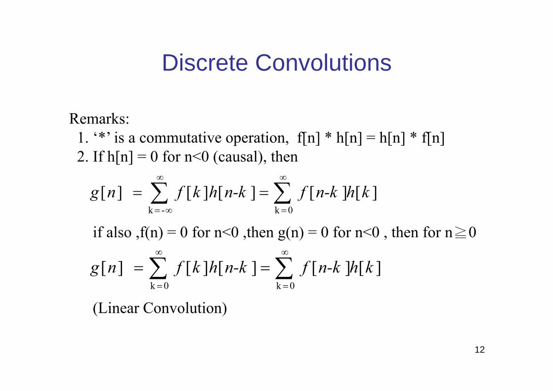
Discrete Convolutions

][][ ][][][0k-k

khn-kfn-khkf ng ∑∑∞

=

∞

∞=

==

Remarks:1. ‘*’ is a commutative operation, f[n] * h[n] = h[n] * f[n]2. If h[n] = 0 for n<0 (causal), then

if also ,f(n) = 0 for n<0 ,then g(n) = 0 for n<0 , then for n≧0

(Linear Convolution)

][][ ][][][0k0k

khn-kfn-khkf ng ∑∑∞

=

∞

=

==

12

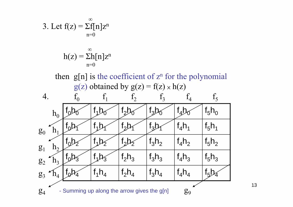
∞3. Let f(z) = Σf[n]zn

n=0

∞h(z) = Σh[n]zn

n=0

then g[n] is the coefficient of zn for the polynomialg(z) obtained by g(z) = f(z) × h(z)

4. f0 f1 f2 f3 f4 f5

h0

g0 h1

g1 h2

g2 h3

g3 h4

g4 - Summing up along the arrow gives the g[n] g9

f0h0 f1h0 f2h0 f3h0 f4h0 f5h0

f0h1 f1h1 f2h1 f3h1 f4h1 f5h1

f0h2 f1h2 f2h2 f3h2 f4h2 f5h2

f0h3 f1h3 f2h3 f3h3 f4h3 f5h3

f0h4 f1h4 f2h4 f3h4 f4h4 f5h4

13

• Can you use only 3 multiplications to find g0, g1 and g2?– g0=f0h0

– g1=f1h1

– a0=(f0+f1)– a1=(h0+h1)– g1=a0a1-g0-g1 14

f0h0 f1h0

f0h1 f1h1

f0 f1

g0

g1

g2

5. length f[n] : L1length h[n] : L2length g[n] = L1 + L2 –1

15

Multiplication v.s. Convolution

• If   and   , and let   .• Then the polynomials   and   , defined in 3.,

become the binary representations of the two scalars   and   respectively. Then   in 3. becomes the product result of   .

• And in this case, the digital convolution, defined in 4., is equivalent to the multiplication of two scalars.

• Could you extend the above discussion one-dimensional higher? What is the meaning of “convolution of polynomials”?

16

The System Function: for an LTI-system

)( )( ,

)( )(}{][

][)( where

][][

][][][

][

-k-k

-k

zHzHz

zzHzLng

znhzH

rkhrkhr

khn-kfng

rnf

nn-n

-n

-knn-k

n

∀===

=

==

=

=

∑

∑∑

∑

∞

∞=

∞

∞=

∞

∞=

∞

∞=

xAx λ

geometric progression

is also a geometric progression multiplied by H(r)(z-transform)

real or complex ,for which converges.

: system function 17

Remarks of the system function

• H(z) : eigenvalue of an LTI discrete system• H(z) = z-1 : delay element

H(z) = a : multiplier

EX: Consider the recursion equation:6g[n] + 5g[n-1] + g[n-2] = f [n] , H(z) = ?

Sol: Set f [n] = zn, g[n] = H(z)zn

H(z)(6zn + 5zn-1 + zn-2) = zn

H(z) = 1/(6 + 5z-1 + z-2)18

• System in cascade : pipeline

• System in parallel : parallel

19

Convolution Theorem

• g[n] = f [n] * h[n]• G(z) = F(z) · H(z)

Definitions of system function1. H(z) is the z-transform of h[n]2. If f [n] = zn :

H(z) is the coefficients of the resulting response.3. H(z) equals the ratio G(z)/F(z).

20

h(n)H(z)

f(n)F(z)

g(n)=f(n) * h(n)G(z)=F(z) · H(z)

Remarks of Convolution Theorem

1. If F(z) and G(z) are given :H(z) = G(z)/F(z)

System identification2. If G(z) and H(z) are known :

F(z) = G(z)/H(z)Deconvolution / Signal reconstruction(inverse filtering problem)

21

Both Tasks are challenging because their operations involved with the division of polynomials which may lead to system stability problems!!

Tricks for computing Convolution Sum

• Trick 1: Representing sines and cosines in complex exponential form:

⎪⎪⎩

⎪⎪⎨

⎧

=

+=

jeeθ

eeθjθjθ

jθjθ

2-sin

2cos

-

-

22

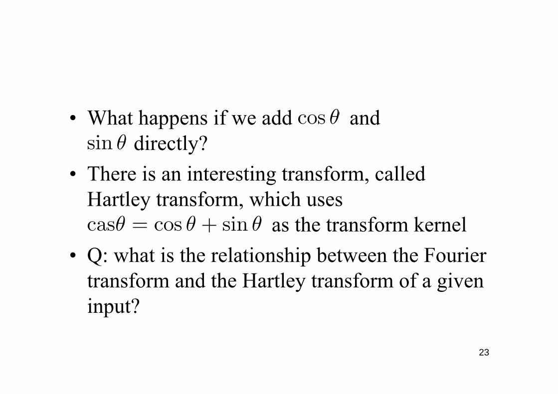
• What happens if we add   and   directly?

• There is an interesting transform, called Hartley transform, which uses   as the transform kernel

• Q: what is the relationship between the Fourier transform and the Hartley transform of a given input?

23

Tricks for computing Convolution Sum

• Trick 2: Infinite and finite summation of exponentials:

⎪⎪⎩

⎪⎪⎨

⎧

=

<=

∑

∑

=

∞

=

α

α

allfor , 1

1

1for , 11

N1

0

0

-α-αα

-αα

N-

n

n

n

n

24

Tricks for computing Convolution Sum

• Trick 3: Balancing equations with complex exponentials:

)2

(sin2

)()1(

2

222

nωje-

-eee-enj

njn-jnjnj

ω

ωωωω

=

=

25

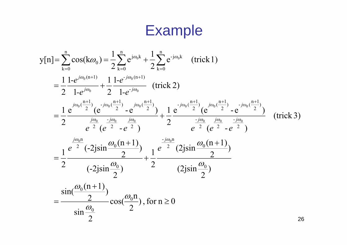
Example

0nfor , )2ncos(

2sin

)2

1)(nsin(

)2

(2jsin

)2

1)(n(2jsin

21

)2

(-2jsin

)2

1)(n(-2jsin

21

3)(trick )-(

)e-(ee21

)-(

)e-(ee21

2)(trick 1

121

11

21

1)(trick e21e

21)cos(ky[n]

0

0

0

0

02n-

0

02n

2-

22-

)2

1n(-)2

1n()2

1n(-

22-

2

)2

1n()2

1n(-)2

1n(

-

1)(n-1)(n

n

0k

kj-n

0k

kjn

0k0

00

000

000

000

000

0

0

0

0

00

≥

+

=

+

+

+

=

+=

+=

+==

++++++

++

===∑∑∑

ωω

ω

ω

ω

ω

ω

ω

ωω

ωωωωωω

ω

ω

ω

ω

ωω

jj

jjj

jωjωjω

jjj

jωjωjω

j

j

j

j

ee

eeeeee

-e-e

-e-e

26