Lecture 17Spatial Data and Cartography (Part 2)

Colin Rundel03/22/2017

1

Plotting

2

Example Data - NC SIDS

nc = st_read(system.file(”shape/nc.shp”, package=”sf”), quiet = TRUE) %>%select(-(AREA:CNTY_ID), -(FIPS:CRESS_ID))

head(nc, n = 10)## Simple feature collection with 10 features and 7 fields## geometry type: MULTIPOLYGON## dimension: XY## bbox: xmin: -81.74107 ymin: 36.07282 xmax: -75.77316 ymax: 36.58965## epsg (SRID): 4267## proj4string: +proj=longlat +datum=NAD27 +no_defs## NAME BIR74 SID74 NWBIR74 BIR79 SID79 NWBIR79## 1 Ashe 1091 1 10 1364 0 19## 2 Alleghany 487 0 10 542 3 12## 3 Surry 3188 5 208 3616 6 260## 4 Currituck 508 1 123 830 2 145## 5 Northampton 1421 9 1066 1606 3 1197## 6 Hertford 1452 7 954 1838 5 1237## 7 Camden 286 0 115 350 2 139## 8 Gates 420 0 254 594 2 371## 9 Warren 968 4 748 1190 2 844## 10 Stokes 1612 1 160 2038 5 176## geometry## 1 MULTIPOLYGON(((-81.47275543...## 2 MULTIPOLYGON(((-81.23989105...## 3 MULTIPOLYGON(((-80.45634460...## 4 MULTIPOLYGON(((-76.00897216...## 5 MULTIPOLYGON(((-77.21766662...## 6 MULTIPOLYGON(((-76.74506378...## 7 MULTIPOLYGON(((-76.00897216...## 8 MULTIPOLYGON(((-76.56250762...## 9 MULTIPOLYGON(((-78.30876159...## 10 MULTIPOLYGON(((-80.02567291...

3

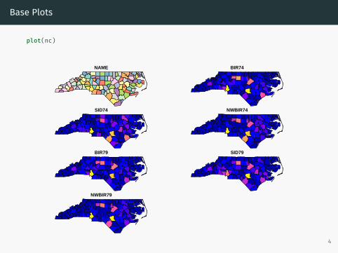
Base Plots

plot(nc)

NAME BIR74

SID74 NWBIR74

BIR79 SID79

NWBIR79

4

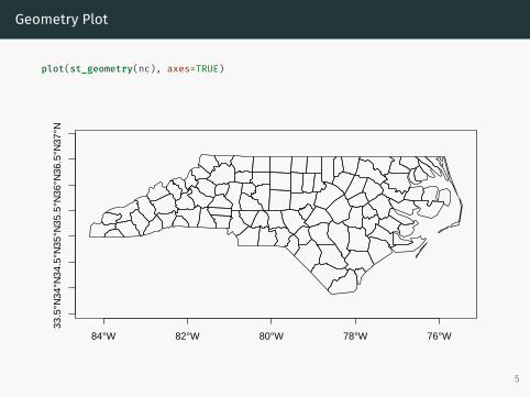
Geometry Plot

plot(st_geometry(nc), axes=TRUE)

84°W 82°W 80°W 78°W 76°W

33.5

°N34

°N34

.5°N

35°N

35.5

°N36

°N36

.5°N

37°N

5

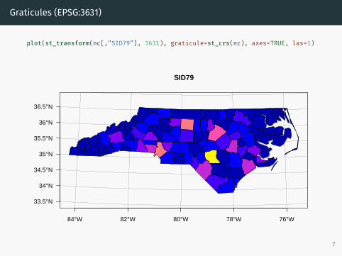
Graticules

plot(nc[,”SID79”], graticule=st_crs(nc), axes=TRUE, las=1)

84°W 82°W 80°W 78°W 76°W

33.5°N

34°N

34.5°N

35°N

35.5°N

36°N

36.5°N

37°N

SID79

6

Graticules (EPSG:3631)

plot(st_transform(nc[,”SID79”], 3631), graticule=st_crs(nc), axes=TRUE, las=1)

84°W 82°W 80°W 78°W 76°W

33.5°N

34°N

34.5°N

35°N

35.5°N

36°N

36.5°N

SID79

7

ggplot2 2.2.1.9 (dev)

ggplot(nc) +geom_sf(aes(fill=SID79 / BIR79))

34°N

34.5°N

35°N

35.5°N

36°N

36.5°N

84°W 82°W 80°W 78°W 76°W

0.000

0.002

0.004

0.006SID79/BIR79

8

ggplot2 + projections

ggplot(st_transform(nc, 3631)) +geom_sf(aes(fill=SID79 / BIR79))

34°N

34.5°N

35°N

35.5°N

36°N

36.5°N

84°W 82°W 80°W 78°W 76°W

0.000

0.002

0.004

0.006SID79/BIR79

9

Example Data - Meuse

data(meuse, meuse.riv, package=”sp”)

meuse = st_as_sf(meuse, coords=c(”x”, ”y”), crs=28992)meuse_riv = st_polygon(list(meuse.riv)) %>% st_sfc() %>% st_set_crs(28992)

meuse## Simple feature collection with 155 features and 12 fields## geometry type: POINT## dimension: XY## bbox: xmin: 178605 ymin: 329714 xmax: 181390 ymax: 333611## epsg (SRID): 28992## proj4string: +proj=sterea +lat_0=52.15616055555555 +lon_0=5.38763888888889 +k=0.9999079 +x_0=155000 +y_0=463000 +ellps=bessel +towgs84=565.4171,50.3319,465.5524,-0.398957,0.343988,-1.87740,4.0725 +units=m +no_defs## First 20 features:## cadmium copper lead zinc elev dist om ffreq soil lime## 1 11.7 85 299 1022 7.909 0.00135803 13.6 1 1 1## 2 8.6 81 277 1141 6.983 0.01222430 14.0 1 1 1## 3 6.5 68 199 640 7.800 0.10302900 13.0 1 1 1## 4 2.6 81 116 257 7.655 0.19009400 8.0 1 2 0## 5 2.8 48 117 269 7.480 0.27709000 8.7 1 2 0## 6 3.0 61 137 281 7.791 0.36406700 7.8 1 2 0## 7 3.2 31 132 346 8.217 0.19009400 9.2 1 2 0## 8 2.8 29 150 406 8.490 0.09215160 9.5 1 1 0## 9 2.4 37 133 347 8.668 0.18461400 10.6 1 1 0## 10 1.6 24 80 183 9.049 0.30970200 6.3 1 2 0## 11 1.4 25 86 189 9.015 0.31511600 6.4 1 2 0## 12 1.8 25 97 251 9.073 0.22812300 9.0 1 1 0## 13 11.2 93 285 1096 7.320 0.00000000 15.4 1 1 1## 14 2.5 31 183 504 8.815 0.11393200 8.4 1 1 0## 15 2.0 27 130 326 8.937 0.16833600 9.1 1 1 0## 16 9.5 86 240 1032 7.702 0.00000000 16.2 1 1 1## 17 7.0 74 133 606 7.160 0.01222430 16.0 1 1 1## 18 7.1 69 148 711 7.100 0.01222430 16.0 1 1 1## 19 8.7 69 207 735 7.020 0.00000000 13.7 1 1 1## 20 12.9 95 284 1052 6.860 0.00000000 14.8 1 1 1## landuse dist.m geometry## 1 Ah 50 POINT(181072 333611)## 2 Ah 30 POINT(181025 333558)## 3 Ah 150 POINT(181165 333537)## 4 Ga 270 POINT(181298 333484)## 5 Ah 380 POINT(181307 333330)## 6 Ga 470 POINT(181390 333260)## 7 Ah 240 POINT(181165 333370)## 8 Ab 120 POINT(181027 333363)## 9 Ab 240 POINT(181060 333231)## 10 W 420 POINT(181232 333168)## 11 Fh 400 POINT(181191 333115)## 12 Ag 300 POINT(181032 333031)## 13 W 20 POINT(180874 333339)## 14 Ah 130 POINT(180969 333252)## 15 Ah 220 POINT(181011 333161)## 16 W 10 POINT(180830 333246)## 17 W 10 POINT(180763 333104)## 18 W 10 POINT(180694 332972)## 19 W 10 POINT(180625 332847)## 20 <NA> 10 POINT(180555 332707)

10

Meuse

plot(meuse, pch=16)

cadmium copper lead zinc elev

dist om ffreq soil lime

11

Layering plots

plot(meuse[,”lead”], pch=16, axes=TRUE)plot(meuse_riv, col=adjustcolor(”lightblue”, alpha.f=0.5), add=TRUE, border = NA)

176000 178000 180000 182000 184000

3300

0033

1000

3320

0033

3000

lead

12

Layering plots (oops)

plot(meuse, pch=16)plot(meuse_riv, col=adjustcolor(”lightblue”, alpha.f=0.5), add=TRUE, border = NA)

cadmium copper lead zinc elev

dist om ffreq soil lime

13

ggplot2

ggplot() +geom_sf(data=st_sf(meuse_riv), fill=”lightblue”, color=NA) +geom_sf(data=meuse, aes(color=lead), size=1)

50.92°N

50.94°N

50.96°N

50.98°N

51°N

51.02°N

5.72°E5.73°E5.74°E5.75°E5.76°E5.77°E

200

400

600

lead

14

ggplot2 - axis limits

ggplot() +geom_sf(data=st_sf(meuse_riv), fill=”lightblue”, color=NA) +geom_sf(data=meuse, aes(color=lead), size=0.1) +ylim(329714, 333611)

50.955°N

50.96°N

50.965°N

50.97°N

50.975°N

50.98°N

50.985°N

50.99°N

5.72°E 5.73°E 5.74°E 5.75°E 5.76°E 5.77°E

200

400

600

lead

15

ggplot2 - bounding box

ggplot() +geom_sf(data=st_sf(meuse_riv), fill=”lightblue”, color=NA) +geom_sf(data=meuse, aes(color=lead), size=0.1) +ylim(st_bbox(meuse)[”ymin”], st_bbox(meuse)[”ymax”])

50.955°N

50.96°N

50.965°N

50.97°N

50.975°N

50.98°N

50.985°N

50.99°N

5.72°E 5.73°E 5.74°E 5.75°E 5.76°E 5.77°E

200

400

600

lead

16

Geometry Manipulation

17

Casting

nc_pts = st_cast(nc, ”MULTIPOINT”)

nc_pts## Simple feature collection with 100 features and 7 fields## geometry type: MULTIPOINT## dimension: XY## bbox: xmin: -84.32385 ymin: 33.88199 xmax: -75.45698 ymax: 36.58965## epsg (SRID): 4267## proj4string: +proj=longlat +datum=NAD27 +no_defs## First 20 features:## NAME BIR74 SID74 NWBIR74 BIR79 SID79 NWBIR79## 1 Ashe 1091 1 10 1364 0 19## 2 Alleghany 487 0 10 542 3 12## 3 Surry 3188 5 208 3616 6 260## 4 Currituck 508 1 123 830 2 145## 5 Northampton 1421 9 1066 1606 3 1197## 6 Hertford 1452 7 954 1838 5 1237## 7 Camden 286 0 115 350 2 139## 8 Gates 420 0 254 594 2 371## 9 Warren 968 4 748 1190 2 844## 10 Stokes 1612 1 160 2038 5 176## 11 Caswell 1035 2 550 1253 2 597## 12 Rockingham 4449 16 1243 5386 5 1369## 13 Granville 1671 4 930 2074 4 1058## 14 Person 1556 4 613 1790 4 650## 15 Vance 2180 4 1179 2753 6 1492## 16 Halifax 3608 18 2365 4463 17 2980## 17 Pasquotank 1638 3 622 2275 4 933## 18 Wilkes 3146 4 200 3725 7 222## 19 Watauga 1323 1 17 1775 1 33## 20 Perquimans 484 1 230 676 0 310## geometry## 1 MULTIPOINT(-81.472755432128...## 2 MULTIPOINT(-81.239891052246...## 3 MULTIPOINT(-80.456344604492...## 4 MULTIPOINT(-76.008972167968...## 5 MULTIPOINT(-77.217666625976...## 6 MULTIPOINT(-76.745063781738...## 7 MULTIPOINT(-76.008972167968...## 8 MULTIPOINT(-76.562507629394...## 9 MULTIPOINT(-78.308761596679...## 10 MULTIPOINT(-80.025672912597...## 11 MULTIPOINT(-79.530509948730...## 12 MULTIPOINT(-79.530509948730...## 13 MULTIPOINT(-78.749122619628...## 14 MULTIPOINT(-78.806800842285...## 15 MULTIPOINT(-78.492523193359...## 16 MULTIPOINT(-77.332206726074...## 17 MULTIPOINT(-76.298927307128...## 18 MULTIPOINT(-81.020568847656...## 19 MULTIPOINT(-81.806221008300...## 20 MULTIPOINT(-76.480529785156...

18

plot(st_geometry(nc), border=’grey’)plot(st_geometry(nc_pts), pch=16, cex=0.5, add=TRUE)

19

Casting - POINT

st_cast(nc, ”POINT”)## Simple feature collection with 2529 features and 7 fields## geometry type: POINT## dimension: XY## bbox: xmin: -84.32385 ymin: 33.88199 xmax: -75.45698 ymax: 36.58965## epsg (SRID): 4267## proj4string: +proj=longlat +datum=NAD27 +no_defs## First 20 features:## NAME BIR74 SID74 NWBIR74 BIR79 SID79 NWBIR79## 1 Ashe 1091 1 10 1364 0 19## 2 Ashe 1091 1 10 1364 0 19## 3 Ashe 1091 1 10 1364 0 19## 4 Ashe 1091 1 10 1364 0 19## 5 Ashe 1091 1 10 1364 0 19## 6 Ashe 1091 1 10 1364 0 19## 7 Ashe 1091 1 10 1364 0 19## 8 Ashe 1091 1 10 1364 0 19## 9 Ashe 1091 1 10 1364 0 19## 10 Ashe 1091 1 10 1364 0 19## 11 Ashe 1091 1 10 1364 0 19## 12 Ashe 1091 1 10 1364 0 19## 13 Ashe 1091 1 10 1364 0 19## 14 Ashe 1091 1 10 1364 0 19## 15 Ashe 1091 1 10 1364 0 19## 16 Ashe 1091 1 10 1364 0 19## 17 Ashe 1091 1 10 1364 0 19## 18 Ashe 1091 1 10 1364 0 19## 19 Ashe 1091 1 10 1364 0 19## 20 Ashe 1091 1 10 1364 0 19## geometry## 1 POINT(-81.4727554321289 36....## 2 POINT(-81.5408401489258 36....## 3 POINT(-81.5619812011719 36....## 4 POINT(-81.6330642700195 36....## 5 POINT(-81.7410736083984 36....## 6 POINT(-81.6982803344727 36....## 7 POINT(-81.7027969360352 36....## 8 POINT(-81.6699981689453 36....## 9 POINT(-81.3452987670898 36....## 10 POINT(-81.347541809082 36.5...## 11 POINT(-81.3247756958008 36....## 12 POINT(-81.3133239746094 36....## 13 POINT(-81.2662353515625 36....## 14 POINT(-81.2628402709961 36....## 15 POINT(-81.2406921386719 36....## 16 POINT(-81.2398910522461 36....## 17 POINT(-81.2642440795898 36....## 18 POINT(-81.3289947509766 36....## 19 POINT(-81.3613739013672 36....## 20 POINT(-81.3656921386719 36....

20

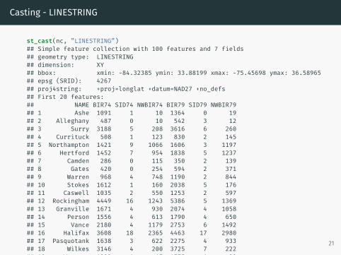
Casting - LINESTRING

st_cast(nc, ”LINESTRING”)## Simple feature collection with 100 features and 7 fields## geometry type: LINESTRING## dimension: XY## bbox: xmin: -84.32385 ymin: 33.88199 xmax: -75.45698 ymax: 36.58965## epsg (SRID): 4267## proj4string: +proj=longlat +datum=NAD27 +no_defs## First 20 features:## NAME BIR74 SID74 NWBIR74 BIR79 SID79 NWBIR79## 1 Ashe 1091 1 10 1364 0 19## 2 Alleghany 487 0 10 542 3 12## 3 Surry 3188 5 208 3616 6 260## 4 Currituck 508 1 123 830 2 145## 5 Northampton 1421 9 1066 1606 3 1197## 6 Hertford 1452 7 954 1838 5 1237## 7 Camden 286 0 115 350 2 139## 8 Gates 420 0 254 594 2 371## 9 Warren 968 4 748 1190 2 844## 10 Stokes 1612 1 160 2038 5 176## 11 Caswell 1035 2 550 1253 2 597## 12 Rockingham 4449 16 1243 5386 5 1369## 13 Granville 1671 4 930 2074 4 1058## 14 Person 1556 4 613 1790 4 650## 15 Vance 2180 4 1179 2753 6 1492## 16 Halifax 3608 18 2365 4463 17 2980## 17 Pasquotank 1638 3 622 2275 4 933## 18 Wilkes 3146 4 200 3725 7 222## 19 Watauga 1323 1 17 1775 1 33## 20 Perquimans 484 1 230 676 0 310## geometry## 1 LINESTRING(-81.472755432128...## 2 LINESTRING(-81.239891052246...## 3 LINESTRING(-80.456344604492...## 4 LINESTRING(-76.008972167968...## 5 LINESTRING(-77.217666625976...## 6 LINESTRING(-76.745063781738...## 7 LINESTRING(-76.008972167968...## 8 LINESTRING(-76.562507629394...## 9 LINESTRING(-78.308761596679...## 10 LINESTRING(-80.025672912597...## 11 LINESTRING(-79.530509948730...## 12 LINESTRING(-79.530509948730...## 13 LINESTRING(-78.749122619628...## 14 LINESTRING(-78.806800842285...## 15 LINESTRING(-78.492523193359...## 16 LINESTRING(-77.332206726074...## 17 LINESTRING(-76.298927307128...## 18 LINESTRING(-81.020568847656...## 19 LINESTRING(-81.806221008300...## 20 LINESTRING(-76.480529785156...

21

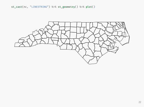
st_cast(nc, ”LINESTRING”) %>% st_geometry() %>% plot()

22

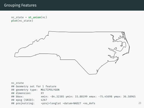
Grouping Features

nc_state = st_union(nc)plot(nc_state)

nc_state## Geometry set for 1 feature## geometry type: MULTIPOLYGON## dimension: XY## bbox: xmin: -84.32385 ymin: 33.88199 xmax: -75.45698 ymax: 36.58965## epsg (SRID): 4267## proj4string: +proj=longlat +datum=NAD27 +no_defs 23

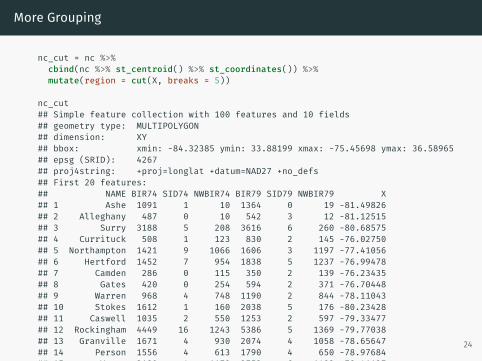
More Grouping

nc_cut = nc %>%cbind(nc %>% st_centroid() %>% st_coordinates()) %>%mutate(region = cut(X, breaks = 5))

nc_cut## Simple feature collection with 100 features and 10 fields## geometry type: MULTIPOLYGON## dimension: XY## bbox: xmin: -84.32385 ymin: 33.88199 xmax: -75.45698 ymax: 36.58965## epsg (SRID): 4267## proj4string: +proj=longlat +datum=NAD27 +no_defs## First 20 features:## NAME BIR74 SID74 NWBIR74 BIR79 SID79 NWBIR79 X## 1 Ashe 1091 1 10 1364 0 19 -81.49826## 2 Alleghany 487 0 10 542 3 12 -81.12515## 3 Surry 3188 5 208 3616 6 260 -80.68575## 4 Currituck 508 1 123 830 2 145 -76.02750## 5 Northampton 1421 9 1066 1606 3 1197 -77.41056## 6 Hertford 1452 7 954 1838 5 1237 -76.99478## 7 Camden 286 0 115 350 2 139 -76.23435## 8 Gates 420 0 254 594 2 371 -76.70448## 9 Warren 968 4 748 1190 2 844 -78.11043## 10 Stokes 1612 1 160 2038 5 176 -80.23428## 11 Caswell 1035 2 550 1253 2 597 -79.33477## 12 Rockingham 4449 16 1243 5386 5 1369 -79.77038## 13 Granville 1671 4 930 2074 4 1058 -78.65647## 14 Person 1556 4 613 1790 4 650 -78.97684## 15 Vance 2180 4 1179 2753 6 1492 -78.41127## 16 Halifax 3608 18 2365 4463 17 2980 -77.65628## 17 Pasquotank 1638 3 622 2275 4 933 -76.31460## 18 Wilkes 3146 4 200 3725 7 222 -81.15963## 19 Watauga 1323 1 17 1775 1 33 -81.69129## 20 Perquimans 484 1 230 676 0 310 -76.45461## Y region geometry## 1 36.43140 (-82.4,-80.8] MULTIPOLYGON(((-81.47275543...## 2 36.49101 (-82.4,-80.8] MULTIPOLYGON(((-81.23989105...## 3 36.41252 (-80.8,-79.1] MULTIPOLYGON(((-80.45634460...## 4 36.40728 (-77.5,-75.8] MULTIPOLYGON(((-76.00897216...## 5 36.42228 (-77.5,-75.8] MULTIPOLYGON(((-77.21766662...## 6 36.36145 (-77.5,-75.8] MULTIPOLYGON(((-76.74506378...## 7 36.40120 (-77.5,-75.8] MULTIPOLYGON(((-76.00897216...## 8 36.44423 (-77.5,-75.8] MULTIPOLYGON(((-76.56250762...## 9 36.39697 (-79.1,-77.5] MULTIPOLYGON(((-78.30876159...## 10 36.40034 (-80.8,-79.1] MULTIPOLYGON(((-80.02567291...## 11 36.39347 (-80.8,-79.1] MULTIPOLYGON(((-79.53050994...## 12 36.39600 (-80.8,-79.1] MULTIPOLYGON(((-79.53050994...## 13 36.30013 (-79.1,-77.5] MULTIPOLYGON(((-78.74912261...## 14 36.38870 (-79.1,-77.5] MULTIPOLYGON(((-78.80680084...## 15 36.36234 (-79.1,-77.5] MULTIPOLYGON(((-78.49252319...## 16 36.25305 (-79.1,-77.5] MULTIPOLYGON(((-77.33220672...## 17 36.31237 (-77.5,-75.8] MULTIPOLYGON(((-76.29892730...## 18 36.20160 (-82.4,-80.8] MULTIPOLYGON(((-81.02056884...## 19 36.22480 (-82.4,-80.8] MULTIPOLYGON(((-81.80622100...## 20 36.20488 (-77.5,-75.8] MULTIPOLYGON(((-76.48052978...

24

ggplot(nc_cut) +geom_sf(aes(fill=region))

34°N

34.5°N

35°N

35.5°N

36°N

36.5°N

84°W 82°W 80°W 78°W 76°W

region

(−84.1,−82.4]

(−82.4,−80.8]

(−80.8,−79.1]

(−79.1,−77.5]

(−77.5,−75.8]

25

dplyr and sf - BFFs

nc_cut %>%group_by(region) %>%summarize(geometry = st_union(geometry)) %>%ggplot() + geom_sf(aes(fill=region))

34°N

34.5°N

35°N

35.5°N

36°N

36.5°N

84°W 82°W 80°W 78°W 76°W

region

(−84.1,−82.4]

(−82.4,−80.8]

(−80.8,−79.1]

(−79.1,−77.5]

(−77.5,−75.8]

26

Affine Transfomations

rotate = function(a) matrix(c(cos(a), sin(a), -sin(a), cos(a)), 2, 2)

ctrd = st_centroid(nc_state)state_rotate = (nc_state - ctrd) * rotate(-pi/4) + ctrdplot(state_rotate, axes=TRUE)

−85 −80 −75

3233

3435

3637

3839

27

Scaling Size

ctrd = st_geometry(st_centroid(nc))area = st_area(nc) %>% strip_attrs()nc_scaled = ncfor(i in 1:nrow(nc))nc_scaled$geometry[[i]] = ((st_geometry(nc[i,]) - ctrd[i]) *

sqrt(min(area)/area[i]) + ctrd[i])[[1]]

plot(nc_scaled[,”SID79”])

SID79

28

Back to the highways

hwy = st_read(”../../data/gis/us_interstates/”, quiet=TRUE, stringsAsFactors=FALSE) %>% st_transform(st_crs(nc))

ggplot() +geom_sf(data=nc) +geom_sf(data=hwy, col=’red’)

20°N

30°N

40°N

50°N

60°N

160°W 140°W 120°W 100°W 80°W

29

NC Interstate Highways

hwy_nc = st_intersection(hwy, nc)

ggplot() +geom_sf(data=nc) +geom_sf(data=hwy_nc, col=’red’)

34°N

34.5°N

35°N

35.5°N

36°N

36.5°N

84°W 82°W 80°W 78°W 76°W

hwy_nc## Simple feature collection with 56 features and 10 fields## geometry type: GEOMETRY## dimension: XY## bbox: xmin: -83.09008 ymin: 34.2791 xmax: -77.57348 ymax: 36.56092## epsg (SRID): 4267## proj4string: +proj=longlat +datum=NAD27 +no_defs## First 20 features:## ROUTE_NUM DIST_MILES DIST_KM NAME BIR74 SID74 NWBIR74 BIR79## 1 I77 546.83 880.05 Surry 3188 5 208 3616## 2 I95 1829.69 2944.61 Northampton 1421 9 1066 1606## 3 I85 610.51 982.53 Warren 968 4 748 1190## 4 I85 610.51 982.53 Granville 1671 4 930 2074## 5 I85 610.51 982.53 Vance 2180 4 1179 2753## 6 I95 1829.69 2944.61 Halifax 3608 18 2365 4463## 7 I77 546.83 880.05 Yadkin 1269 1 65 1568## 8 I40 2480.59 3992.14 Forsyth 11858 10 3919 15704## 9 I40 F 18.33 29.49 Forsyth 11858 10 3919 15704## 10 I40 2480.59 3992.14 Guilford 16184 23 5483 20543## 11 I40 F 18.33 29.49 Guilford 16184 23 5483 20543## 12 I73 54.84 88.25 Guilford 16184 23 5483 20543## 13 I85 610.51 982.53 Guilford 16184 23 5483 20543## 14 I40 2480.59 3992.14 Alamance 4672 13 1243 5767## 15 I85 610.51 982.53 Alamance 4672 13 1243 5767## 16 I40 2480.59 3992.14 Orange 3164 4 776 4478## 17 I85 610.51 982.53 Orange 3164 4 776 4478## 18 I40 2480.59 3992.14 Durham 7970 16 3732 10432## 19 I85 610.51 982.53 Durham 7970 16 3732 10432## 20 I95 1829.69 2944.61 Nash 4021 8 1851 5189## SID79 NWBIR79 geoms## 1 6 260 LINESTRING(-80.745014063930...## 2 3 1197 LINESTRING(-77.57347527372 ...## 3 2 844 LINESTRING(-78.303117397331...## 4 4 1058 LINESTRING(-78.788842681252...## 5 6 1492 LINESTRING(-78.515924528417...## 6 17 2980 LINESTRING(-77.629052087089...## 7 1 76 LINESTRING(-80.819025924954...## 8 18 5031 LINESTRING(-80.425019190468...## 9 18 5031 LINESTRING(-80.325561526296...## 10 38 7089 LINESTRING(-80.007026428880...## 11 38 7089 LINESTRING(-80.033752259421...## 12 38 7089 LINESTRING(-79.826140362816...## 13 38 7089 LINESTRING(-79.804892355469...## 14 11 1397 MULTILINESTRING((-79.259665...## 15 11 1397 LINESTRING(-79.261130125158...## 16 6 1086 LINESTRING(-79.259586126259...## 17 6 1086 LINESTRING(-79.125632056119...## 18 22 4948 LINESTRING(-79.001499734474...## 19 22 4948 LINESTRING(-78.986039485815...## 20 7 2274 LINESTRING(-77.786676909027...

30

Counties near the interstate (Projection)

nc_utm = st_transform(nc, ”+proj=utm +zone=17 +datum=NAD83 +units=m +no_defs”)hwy_utm = st_transform(hwy, ”+proj=utm +zone=17 +datum=NAD83 +units=m +no_defs”)

hwy_nc_utm = st_intersection(nc_utm, hwy_utm)

ggplot() +geom_sf(data=nc_utm) +geom_sf(data=hwy_nc_utm, col=’red’)

34°N

34.5°N

35°N

35.5°N

36°N

36.5°N

84°W 82°W 80°W 78°W 76°W

31

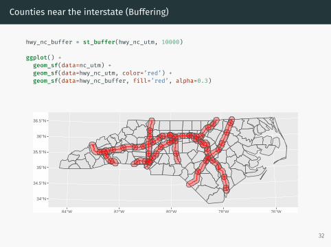
Counties near the interstate (Buffering)

hwy_nc_buffer = st_buffer(hwy_nc_utm, 10000)

ggplot() +geom_sf(data=nc_utm) +geom_sf(data=hwy_nc_utm, color=’red’) +geom_sf(data=hwy_nc_buffer, fill=’red’, alpha=0.3)

34°N

34.5°N

35°N

35.5°N

36°N

36.5°N

84°W 82°W 80°W 78°W 76°W

32

Counties near the interstate (Buffering + Union)

hwy_nc_buffer = st_buffer(hwy_nc_utm, 10000) %>% st_union() %>% st_sf()

ggplot() +geom_sf(data=nc_utm) +geom_sf(data=hwy_nc_utm, color=’red’) +geom_sf(data=hwy_nc_buffer, fill=’red’, alpha=0.3)

34°N

34.5°N

35°N

35.5°N

36°N

36.5°N

84°W 82°W 80°W 78°W 76°W

33

Exercise 1

How many counties in North Carolina are within 5, 10, 20, or 50 km of aninterstate highway?

34

Raster Data

35

Example data - Meuse

meuse_rast = raster(system.file(”external/test.grd”, package=”raster”))

meuse_rast## class : RasterLayer## dimensions : 115, 80, 9200 (nrow, ncol, ncell)## resolution : 40, 40 (x, y)## extent : 178400, 181600, 329400, 334000 (xmin, xmax, ymin, ymax)## coord. ref. : +init=epsg:28992 +towgs84=565.237,50.0087,465.658,-0.406857,0.350733,-1.87035,4.0812 +proj=sterea +lat_0=52.15616055555555 +lon_0=5.38763888888889 +k=0.9999079 +x_0=155000 +y_0=463000 +ellps=bessel +units=m +no_defs## data source : /usr/local/lib/R/3.3/site-library/raster/external/test.grd## names : test## values : 128.434, 1805.78 (min, max)

36

plot(meuse_rast)plot(meuse_riv, add=TRUE, col=adjustcolor(”lightblue”,alpha.f = 0.5), border=NA)

176000 178000 180000 182000 184000

3300

0033

2000

3340

00

500

1000

1500

37

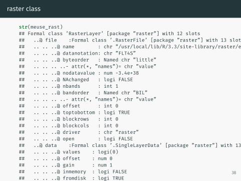
raster class

str(meuse_rast)## Formal class ’RasterLayer’ [package ”raster”] with 12 slots## ..@ file :Formal class ’.RasterFile’ [package ”raster”] with 13 slots## .. .. ..@ name : chr ”/usr/local/lib/R/3.3/site-library/raster/external/test.grd”## .. .. ..@ datanotation: chr ”FLT4S”## .. .. ..@ byteorder : Named chr ”little”## .. .. .. ..- attr(*, ”names”)= chr ”value”## .. .. ..@ nodatavalue : num -3.4e+38## .. .. ..@ NAchanged : logi FALSE## .. .. ..@ nbands : int 1## .. .. ..@ bandorder : Named chr ”BIL”## .. .. .. ..- attr(*, ”names”)= chr ”value”## .. .. ..@ offset : int 0## .. .. ..@ toptobottom : logi TRUE## .. .. ..@ blockrows : int 0## .. .. ..@ blockcols : int 0## .. .. ..@ driver : chr ”raster”## .. .. ..@ open : logi FALSE## ..@ data :Formal class ’.SingleLayerData’ [package ”raster”] with 13 slots## .. .. ..@ values : logi(0)## .. .. ..@ offset : num 0## .. .. ..@ gain : num 1## .. .. ..@ inmemory : logi FALSE## .. .. ..@ fromdisk : logi TRUE## .. .. ..@ isfactor : logi FALSE## .. .. ..@ attributes: list()## .. .. ..@ haveminmax: logi TRUE## .. .. ..@ min : num 128## .. .. ..@ max : num 1806## .. .. ..@ band : int 1## .. .. ..@ unit : chr ””## .. .. ..@ names : chr ”test”## ..@ legend :Formal class ’.RasterLegend’ [package ”raster”] with 5 slots## .. .. ..@ type : chr(0)## .. .. ..@ values : logi(0)## .. .. ..@ color : logi(0)## .. .. ..@ names : logi(0)## .. .. ..@ colortable: logi(0)## ..@ title : chr(0)## ..@ extent :Formal class ’Extent’ [package ”raster”] with 4 slots## .. .. ..@ xmin: num 178400## .. .. ..@ xmax: num 181600## .. .. ..@ ymin: num 329400## .. .. ..@ ymax: num 334000## ..@ rotated : logi FALSE## ..@ rotation:Formal class ’.Rotation’ [package ”raster”] with 2 slots## .. .. ..@ geotrans: num(0)## .. .. ..@ transfun:function ()## ..@ ncols : int 80## ..@ nrows : int 115## ..@ crs :Formal class ’CRS’ [package ”sp”] with 1 slot## .. .. ..@ projargs: chr ”+init=epsg:28992 +towgs84=565.237,50.0087,465.658,-0.406857,0.350733,-1.87035,4.0812 +proj=sterea +lat_0=52.15616055555555 +lon”| __truncated__## ..@ history : list()## ..@ z : list()

38

raster features

extent(meuse_rast)## class : Extent## xmin : 178400## xmax : 181600## ymin : 329400## ymax : 334000

dim(meuse_rast)## [1] 115 80 1

res(meuse_rast)## [1] 40 40

projection(meuse_rast)## [1] ”+init=epsg:28992 +towgs84=565.237,50.0087,465.658,-0.406857,0.350733,-1.87035,4.0812 +proj=sterea +lat_0=52.15616055555555 +lon_0=5.38763888888889 +k=0.9999079 +x_0=155000 +y_0=463000 +ellps=bessel +units=m +no_defs”

meuse_rast[20,]## [1] NA NA NA NA NA NA NA NA## [9] NA NA NA NA NA NA NA NA## [17] NA NA NA NA NA NA NA NA## [25] NA NA NA NA NA NA NA NA## [33] NA NA NA NA NA NA NA NA## [41] NA NA NA NA NA NA NA NA## [49] NA NA NA NA NA NA NA NA## [57] NA NA NA 749.536 895.292 791.145 607.186 511.044## [65] 468.404 399.325 350.362 306.180 300.483 310.082 283.940 285.771## [73] 304.709 309.690 301.799 308.753 328.357 345.611 NA NA

39

Rasters and Projections

meuse_rast_ll = projectRaster(meuse_rast, crs=”+proj=longlat +datum=NAD27 +no_defs”)

par(mfrow=c(1,2))plot(meuse_rast)plot(meuse_rast_ll)

178500 180000 181500

3300

0033

2000

3340

00

500

1000

1500

5.72 5.74 5.76

50.9

650

.97

50.9

850

.99

500

1000

1500

40

meuse_rast## class : RasterLayer## dimensions : 115, 80, 9200 (nrow, ncol, ncell)## resolution : 40, 40 (x, y)## extent : 178400, 181600, 329400, 334000 (xmin, xmax, ymin, ymax)## coord. ref. : +init=epsg:28992 +towgs84=565.237,50.0087,465.658,-0.406857,0.350733,-1.87035,4.0812 +proj=sterea +lat_0=52.15616055555555 +lon_0=5.38763888888889 +k=0.9999079 +x_0=155000 +y_0=463000 +ellps=bessel +units=m +no_defs## data source : /usr/local/lib/R/3.3/site-library/raster/external/test.grd## names : test## values : 128.434, 1805.78 (min, max)

meuse_rast_ll## class : RasterLayer## dimensions : 131, 91, 11921 (nrow, ncol, ncell)## resolution : 0.000569, 0.00036 (x, y)## extent : 5.717362, 5.769141, 50.95089, 50.99805 (xmin, xmax, ymin, ymax)## coord. ref. : +proj=longlat +datum=NAD27 +no_defs +ellps=clrk66 +nadgrids=@conus,@alaska,@ntv2_0.gsb,@ntv1_can.dat## data source : in memory## names : test## values : 135.647, 1693.578 (min, max)

41

Simple Features←→ Rasters

meuse_riv_rast = rasterize(meuse_riv, meuse_rast)## Error in (function (classes, fdef, mtable) : unable to find an inherited method for function ’rasterize’ for signature ’”sfc_POLYGON”, ”RasterLayer”’

meuse_riv_rast = rasterize(as(meuse_riv, ”Spatial”), meuse_rast)plot(meuse_riv_rast)

176000 178000 180000 182000 184000

3300

0033

2000

3340

00

0.9990

0.9995

1.0000

1.0005

1.0010

42

sub = !is.na(meuse_riv_rast[]) & !is.na(meuse_rast[])

river_obs = meuse_rastriver_obs[!sub] = NA

plot(river_obs)

176000 178000 180000 182000 184000

3300

0033

2000

3340

00

400

600

800

1000

1200

1400

xyFromCell(river_obs, which(sub))## x y## [1,] 180420 332540## [2,] 180380 332500## [3,] 180340 332460## [4,] 180300 332420## [5,] 180260 332380## [6,] 180140 332340## [7,] 180180 332340## [8,] 180220 332340## [9,] 180020 332300## [10,] 180060 332300## [11,] 180100 332300## [12,] 179860 332260## [13,] 179900 332260## [14,] 179940 332260## [15,] 179700 332220## [16,] 179740 332220## [17,] 179780 332220## [18,] 179820 332220## [19,] 179660 332180## [20,] 179700 332180## [21,] 179740 332180## [22,] 179620 332140## [23,] 179660 332140## [24,] 179700 332140## [25,] 179580 332100## [26,] 179620 332100## [27,] 179660 332100## [28,] 179580 332060## [29,] 179540 332020## [30,] 179540 331980## [31,] 179500 331900## [32,] 179460 331740## [33,] 179420 331580## [34,] 179380 331500## [35,] 179340 331420## [36,] 179300 331380## [37,] 179260 331340## [38,] 179220 331300## [39,] 179260 331300## [40,] 179180 331260## [41,] 179220 331260## [42,] 179140 331220## [43,] 179180 331220## [44,] 179140 331180## [45,] 179100 331140## [46,] 178900 330940## [47,] 178860 330900## [48,] 178820 330860## [49,] 178580 330540## [50,] 178540 330500## [51,] 178540 330460## [52,] 178500 330420## [53,] 178500 330380## [54,] 180180 330300## [55,] 180220 330300## [56,] 180020 330260## [57,] 180060 330260## [58,] 180100 330260## [59,] 180300 330260## [60,] 180340 330260## [61,] 180380 330260## [62,] 179940 330220## [63,] 179980 330220## [64,] 178460 330180## [65,] 179900 330180## [66,] 179940 330180## [67,] 178460 330140## [68,] 179860 330140## [69,] 179900 330140## [70,] 179860 330100## [71,] 179820 330060## [72,] 179780 330020## [73,] 179740 329980## [74,] 179700 329940## [75,] 179740 329940## [76,] 179660 329900## [77,] 179700 329900## [78,] 178540 329860## [79,] 179620 329860## [80,] 179660 329860## [81,] 178580 329820## [82,] 179580 329820## [83,] 179620 329820## [84,] 178620 329780## [85,] 179540 329780## [86,] 179580 329780## [87,] 178660 329740## [88,] 179500 329740## [89,] 179540 329740## [90,] 179420 329700## [91,] 179460 329700## [92,] 178780 329660## [93,] 179340 329660## [94,] 179380 329660

43

Rasters and Spatial Models

head(meuse)## Simple feature collection with 6 features and 12 fields## geometry type: POINT## dimension: XY## bbox: xmin: 181025 ymin: 333260 xmax: 181390 ymax: 333611## epsg (SRID): 28992## proj4string: +proj=sterea +lat_0=52.15616055555555 +lon_0=5.38763888888889 +k=0.9999079 +x_0=155000 +y_0=463000 +ellps=bessel +towgs84=565.4171,50.3319,465.5524,-0.398957,0.343988,-1.87740,4.0725 +units=m +no_defs## cadmium copper lead zinc elev dist om ffreq soil lime## 1 11.7 85 299 1022 7.909 0.00135803 13.6 1 1 1## 2 8.6 81 277 1141 6.983 0.01222430 14.0 1 1 1## 3 6.5 68 199 640 7.800 0.10302900 13.0 1 1 1## 4 2.6 81 116 257 7.655 0.19009400 8.0 1 2 0## 5 2.8 48 117 269 7.480 0.27709000 8.7 1 2 0## 6 3.0 61 137 281 7.791 0.36406700 7.8 1 2 0## landuse dist.m geometry## 1 Ah 50 POINT(181072 333611)## 2 Ah 30 POINT(181025 333558)## 3 Ah 150 POINT(181165 333537)## 4 Ga 270 POINT(181298 333484)## 5 Ah 380 POINT(181307 333330)## 6 Ga 470 POINT(181390 333260)

head(st_coordinates(meuse))## X Y## 1 181072 333611## 2 181025 333558## 3 181165 333537## 4 181298 333484## 5 181307 333330## 6 181390 333260

44

library(fields)

tps = Tps(x = st_coordinates(meuse), Y=meuse$elev)pred_grid = xyFromCell(meuse_rast, seq_along(meuse_rast))

meuse_elev_pred = meuse_rastmeuse_elev_pred[] = predict(tps, pred_grid)

plot(meuse_elev_pred)

176000 178000 180000 182000 184000

3300

0033

2000

3340

00

3456789

45

Hacky Crap

p = rasterToPolygons(meuse_elev_pred) %>% st_as_sf()grid.arrange(

ggplot() + geom_sf(data=meuse, aes(color=elev), size=0.1),ggplot() + geom_sf(data=p, aes(fill=test), color=NA),ncol=2

)

50.955°N

50.96°N

50.965°N

50.97°N

50.975°N

50.98°N

50.985°N

50.99°N

5.73°E 5.74°E 5.75°E 5.76°E

6

7

8

9

10

elev

50.96°N

50.97°N

50.98°N

50.99°N

5.72°E 5.73°E 5.74°E 5.75°E 5.76°E

4

6

8

test

46