lecture05 - sl - rbfnn svm knn & dt · 23 lecture 05: sl -rbfnn, svm, k-nn and dt the wools...
TRANSCRIPT

Machine Learning
Lecture 5
Supervised Learning
RBFNN, SVM, k-nn and DT
Dr. Patrick [email protected]
South China University of Technology, China
1
Dr. Patrick Chan @ SCUT
Agenda
Radial Basis Function Neural Network
Support Vector Machine
K-Nearest Neighbor
Decision Tree
Lecture 05: SL - RBFNN, SVM, k-nn and DT2
Dr. Patrick Chan @ SCUT
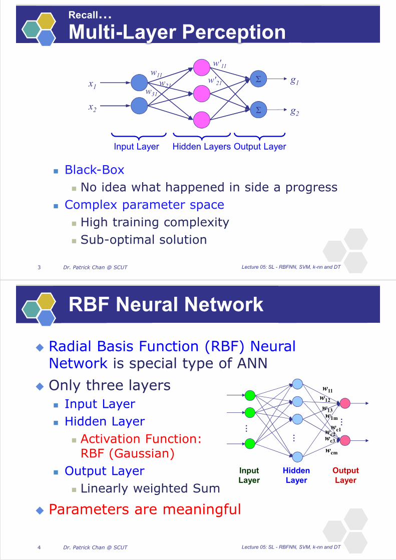
Recall…
Multi-Layer Perception
Black-Box
No idea what happened in side a progress
Complex parameter space
High training complexity
Sub-optimal solution
x1
x2
w11w21
Input Layer Output Layer
Σ
Σ g1
g2
Hidden Layers
w31
w'11
w'21
Lecture 05: SL - RBFNN, SVM, k-nn and DT3
Dr. Patrick Chan @ SCUT
RBF Neural Network
Radial Basis Function (RBF) Neural Network is special type of ANN
Only three layers
Input Layer
Hidden Layer
Activation Function:RBF (Gaussian)
Output Layer
Linearly weighted Sum
Parameters are meaningful
…
…
…
Input
Layer
Hidden
Layer
Output
Layer
w11
w12
w13
w1m
wc1w
c2wc3
wcm
Lecture 05: SL - RBFNN, SVM, k-nn and DT4

Dr. Patrick Chan @ SCUT
RBF Neural Network
Recall, Gaussian function
The most common distribution function
Univariate function:
Two parameters
: mean
: variance
Lecture 05: SL - RBFNN, SVM, k-nn and DT5
Dr. Patrick Chan @ SCUT
RBF Neural Network
Neuron ( ) of RBFNN represents Gaussian Distribution with and Measures the effect of the neuron to x
If the output is large, it means x and the neuron have more similar nature
x
Different center ( )
�
�
Different width ( �)
x
�
�
x is more related to � x is more related to �Lecture 05: SL - RBFNN, SVM, k-nn and DT6

Dr. Patrick Chan @ SCUT
RBF Neural Network
If the weight is larger, the neuron is more important as it has larger effect to the output
Lecture 05: SL - RBFNN, SVM, k-nn and DT7
1
w1=1
�
2 1
w1=1
w2=1
�
�
3 2 1
w1=1
w2=1
w3=0.5
�
�
�
Dr. Patrick Chan @ SCUT
RBF Neural Network
The output of RBFNN for the class k is:
w : the weight
(importance of the neuron)
m : the number of neurons
…
…
…
Input
Layer
Hidden
Layer
Output
Layer
w11
w1cw
21
w2c
w31
w3c
wm1
wmc
�
�
�
�
���
� ���
�
���
Lecture 05: SL - RBFNN, SVM, k-nn and DT8
g1
gc

Dr. Patrick Chan @ SCUT
RBF Neural Network
w3=2
w1=1.5
w2=0.3
Blue Red Red
Lecture 05: SL - RBFNN, SVM, k-nn and DT9
Dr. Patrick Chan @ SCUT
RBF Neural Network
Parameter Determination
Parameters ( , and w) are meaningful
Can be determined by not only gradient descent but also clustering technique
Objective is to seek the “natural” clusters in the data
Clustering will be discussed later in detail
Lecture 05: SL - RBFNN, SVM, k-nn and DT10

Dr. Patrick Chan @ SCUT
RBF Neural Network: Parameter Determination
Gradient Descent
Weights (w)
Centers ( )
Width ( )
�� � �
�� � � �
��� �� � ��
…
…
…
�� ��
��(�) =�����
���exp − 1
2���� �� − ��� ��
���
and
Lecture 05: SL - RBFNN, SVM, k-nn and DT11
Learning rate of parameters can be different
Dr. Patrick Chan @ SCUT
RBF Neural Network: Parameter Determination
Clustering Technique
Given a dataset
Separate samples into groups for each class by clustering technique E.g. K-mean May determine the number of
clusters for each class in advance
Center Mean of samples belonging to
the same cluster
Width Variance of samples belonging
to the same cluster
3 6 180 129 15
15
12
18
0
9
6
3
Lecture 05: SL - RBFNN, SVM, k-nn and DT12

Dr. Patrick Chan @ SCUT
RBF Neural Network: Parameter Determination
Clustering Technique
is fixed when and are determined
RBFNN:
As and are linear relation
Weight (w) can be calculated by
Pseudoinverse (refer to the previous lecture)
Lecture 05: SL - RBFNN, SVM, k-nn and DT13
Dr. Patrick Chan @ SCUT
RBF Neural Network: Parameter Determination
2-Phase Learning
Initialization of gradient descent affects the performance significantly
2-Phase Learning combines clustering and gradient descent
1. Cluster technique initials values of , and w
2. Gradient descent fine-tunes the values
Lecture 05: SL - RBFNN, SVM, k-nn and DT14

Dr. Patrick Chan @ SCUT
RBF Network
How to determine the number of neurons?
Less neurons
Low complexity
Low training cost
More neurons
Represents more complicated distribution
Special CaseMaximum m = training sample # (n)
Mean: a training sample
Covariance: influence of a sample to unseen samples
Lecture 05: SL - RBFNN, SVM, k-nn and DT15
Larger CovSmaller Cov
Dr. Patrick Chan @ SCUT
RBF Neural Network
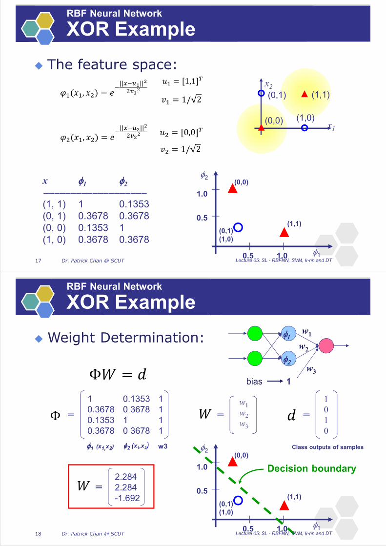
XOR Example
Input space:
Output space:
(1,1)(0,1)
(0,0) (1,0) x1
x2
y10
Lecture 05: SL - RBFNN, SVM, k-nn and DT16
Dr. Patrick Chan @ SCUT
RBF Neural Network
XOR Example
The feature space:
x 1 2(1, 1) 1 0.1353
(0, 1) 0.3678 0.3678
(0, 0) 0.1353 1
(1, 0) 0.3678 0.3678
� � ��|| �!"||
�#"
$� = [1,1](
�
� (
�� � �
�|| �! ||
�#
1
2
1.0
1.0
(0,0)
0.5
0.5(1,1)
(0,1)
(1,0)
(1,1)(0,1)
(0,0) (1,0)x1
x2
Lecture 05: SL - RBFNN, SVM, k-nn and DT17
Dr. Patrick Chan @ SCUT
Weight Determination:
RBF Neural Network
XOR Example
w1
w2
1
w3
bias
1 0.1353 1
0.3678 0 3678 1
0.1353 1 1
0.3678 0 3678 1
=
w1
w2
w3
=
1
0
1
0
=
1
2
1.0
1.0
(0,0)
0.5
0.5(1,1)
(0,1)
(1,0)
2.284
2.284
-1.692
=
Decision boundary
1 (x1,x2) 2 (x1,x2) w3 Class outputs of samples
Lecture 05: SL - RBFNN, SVM, k-nn and DT18
Dr. Patrick Chan @ SCUT
RBF Network: Characteristic
Advantage
RBF Network trains faster than MLP
The hidden layer is easier to interpret than MLP
Disadvantage
During the test phase, the calculation speed ofa neuron in RBF is slower than MLP
Architecture is fixed
Lecture 05: SL - RBFNN, SVM, k-nn and DT19
Dr. Patrick Chan @ SCUT
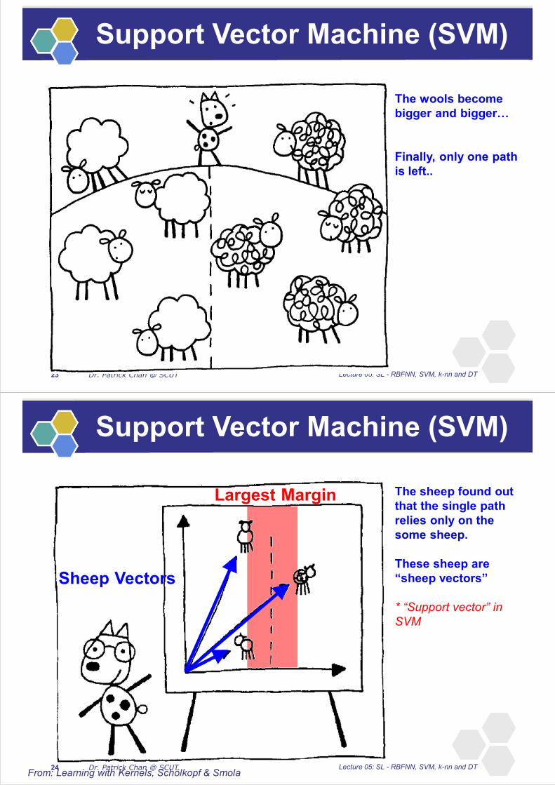
Support Vector Machine (SVM)
Which one is the best linear separator?
Lecture 05: SL - RBFNN, SVM, k-nn and DT20

Dr. Patrick Chan @ SCUT
A clever sheep dog
who was herding his
sheep…
It runs between the
sheep and tries to
separate the black
sheep and white
sheep
Clever
Sheep dog
White
Sheep
Black
Sheep
Support Vector Machine (SVM)
Lecture 05: SL - RBFNN, SVM, k-nn and DT21
Dr. Patrick Chan @ SCUT
Support Vector Machine (SVM)
Lecture 05: SL - RBFNN, SVM, k-nn and DT22
The sheep dog keeps
running…
The sheep start to
grow wools…
The dog feel the gap
between black sheep
and white sheep is
narrower…
Dr. Patrick Chan @ SCUT
Support Vector Machine (SVM)
Lecture 05: SL - RBFNN, SVM, k-nn and DT23
The wools become
bigger and bigger…
Finally, only one path
is left..
Dr. Patrick Chan @ SCUT
Support Vector Machine (SVM)
Lecture 05: SL - RBFNN, SVM, k-nn and DT24From: Learning with Kernels, Schölkopf & Smola
The sheep found out
that the single path
relies only on the
some sheep.
These sheep are
“sheep vectors”
* “Support vector” in
SVM
Largest Margin
Sheep Vectors
Dr. Patrick Chan @ SCUT
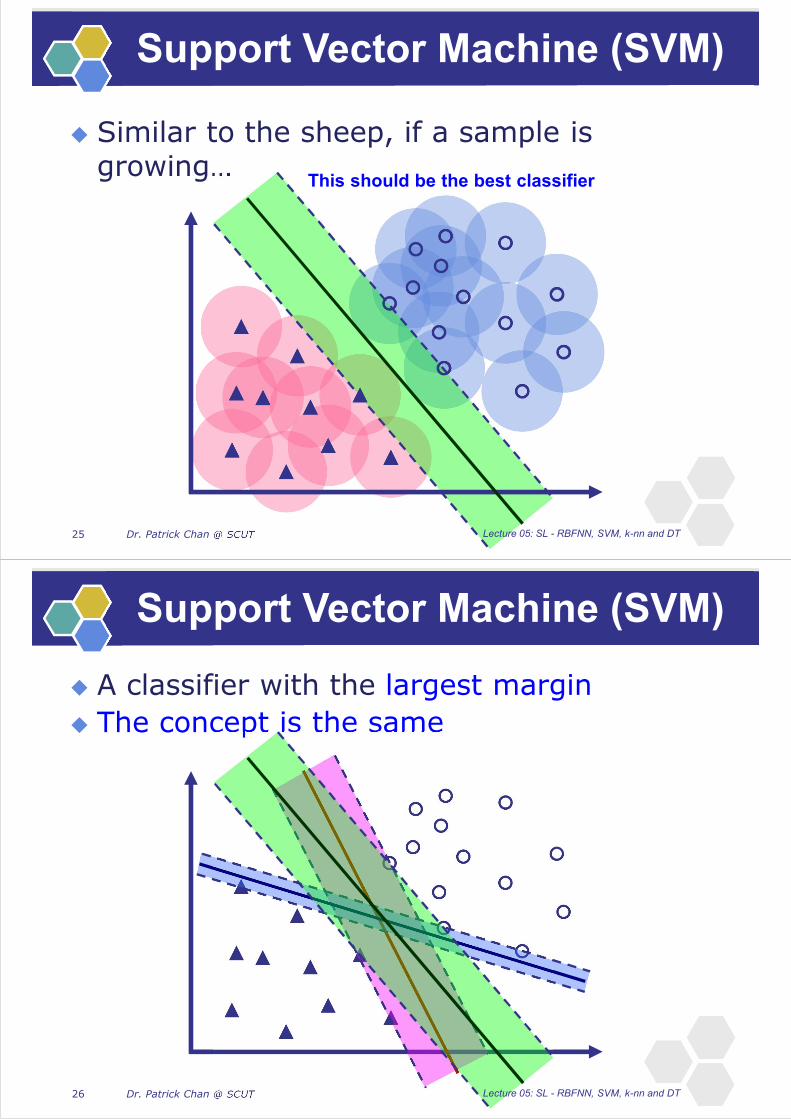
Support Vector Machine (SVM)
Similar to the sheep, if a sample is growing…
This should be the best classifier
Lecture 05: SL - RBFNN, SVM, k-nn and DT25
Dr. Patrick Chan @ SCUT
Support Vector Machine (SVM)
A classifier with the largest margin
The concept is the same
Lecture 05: SL - RBFNN, SVM, k-nn and DT26

Dr. Patrick Chan @ SCUT
Support Vector Machine (SVM)
Maximum Margin Classifier ONLY depends on few samples, called Support Vectors
Support Vectors
Lecture 05: SL - RBFNN, SVM, k-nn and DT27
Dr. Patrick Chan @ SCUT
Support Vector Machine
Statistical Learning Theory
Recall, a classifier is trained by minimizing the training error (Remp, empirical risk)
Our ultimate objective is to minimize the error on unseen sample (R, true risk)
Training error can be reduced easily by using a more complicated classifier
Overfit easily too
A simpler classifier is preferred (assume empirical risk is the same)
Lecture 05: SL - RBFNN, SVM, k-nn and DT28

Dr. Patrick Chan @ SCUT
Support Vector Machine
Statistical Learning Theory
SLT is proposed by Prof. Vladimir Vapnik
Mention the relation between R, Remp and classifier complexity
With 1-η probability, the bound on true risk (R) is:
n = number of training samples
h = VC (Vapnik-Chervonenkis) dimension
Complexity of the classifier
)�*
Complexity
Lecture 05: SL - RBFNN, SVM, k-nn and DT29
Dr. Patrick Chan @ SCUT
Support Vector Machine
Statistical Learning Theory
With 1-η probability, the bound on true risk (R) is:
Observation: When l → ∞, Remp → R
More sample, less complexity
This bound is independent of the sample distribution
Lecture 05: SL - RBFNN, SVM, k-nn and DT30
ComplexityTraining ErrorTrue Error

Dr. Patrick Chan @ SCUT
SVM: Statistical Learning Theory
VC Dimension
VC Dimension for a set of functions { f } is h if there exists a set of h points that can be shattered by { f } but no set of h+1
points
Shattered means that any labeling of the points can be classified correctly by a function from { f }
Larger h = more complicated classifier
Lecture 05: SL - RBFNN, SVM, k-nn and DT31
Dr. Patrick Chan @ SCUT
SVM: SLT: VC Dimension
Linear Classifier Example
2 features
Linear Classifier is a straight line
h is sample #
h=1 h=2 h=3
Yes!
Yes!
Yes!
Lecture 05: SL - RBFNN, SVM, k-nn and DT32

Dr. Patrick Chan @ SCUT
SVM: SLT: VC Dimension
Linear Classifier Example
Maximumvalue of h is 3
Therefore, the VC-Dimensionof Linearclassifier is 3
? ?
h=4
No!
Lecture 05: SL - RBFNN, SVM, k-nn and DT33
Dr. Patrick Chan @ SCUT
Support Vector Machine (SVM)
SVM with a larger margin has a smaller VC dimension
Not only Remp but also the margin is optimized in SVM training
Implicitly optimize R
How to find the boundary?
Separable case
Non-separable case
Slack variables
Kernel method
Lecture 05: SL - RBFNN, SVM, k-nn and DT34
Dr. Patrick Chan @ SCUT
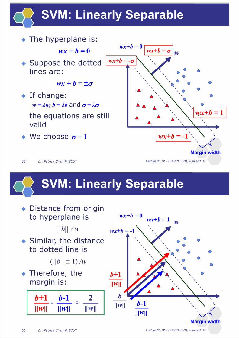
SVM: Linearly Separable
The hyperplane is:
wx + b = 0
Suppose the dotted lines are:
wx + b = ±±±±
If change:
w = λw, b = λb and = λ
the equations are still valid
We choose = 1
Margin width
wwx+b = 0
wx+b = 1
wx+b = -1
wx+b =
wx+b = -
Lecture 05: SL - RBFNN, SVM, k-nn and DT35
Dr. Patrick Chan @ SCUT
SVM: Linearly Separable
Distance from origin to hyperplane is
||b|| / w
Similar, the distance to dotted line is
(||b|| ± 1) /w
Therefore, the margin is:
Margin width
w
b
||w||
wx+b = 0wx+b = 1
wx+b = -1
b-1
||w||
b+1
||w||
b-1
||w||
b+1
||w||
2
||w||- =
Lecture 05: SL - RBFNN, SVM, k-nn and DT36

Dr. Patrick Chan @ SCUT
SVM: Linearly Separable
Problem can be formulated as Quadratic Optimization Problem and solve for w and b
subject to
minimizew, b
w
2Margin width =
where
y(x) = wx+b
y(x) = 1
y(x) = -1
and
Lecture 05: SL - RBFNN, SVM, k-nn and DT37
Dr. Patrick Chan @ SCUT
SVM: Linearly Separable
This optimization problem can be formulated as Dual Problem using
Lagrangian method:
Weight is determined by:
�subject to
Maximumα
� �+
���and
�
� ( �subject to
minimizew, b
Lecture 05: SL - RBFNN, SVM, k-nn and DT38

Dr. Patrick Chan @ SCUT
SVM: Linearly Separable
Many αi are zero
xi with non-zero αi are support vectors (SV) The decision boundary is
determined only by the SV
α1=0.6 α2=0.8
α3=1.4
α4=0 α5=0
α7=0
α8=0
α9=0
α10=0
Non-SV αi=0
α6=0
Lecture 05: SL - RBFNN, SVM, k-nn and DT39
Dr. Patrick Chan @ SCUT
SVM: Linearly Separable
For testing with a new data x
If f(z) > 0, class 1
If f(z) < 0, class 2
Note: w need not be formed explicitly
, , ,
where
Lecture 05: SL - RBFNN, SVM, k-nn and DT40

Dr. Patrick Chan @ SCUT
SVM: Non-Linearly Separable
How about Non-Linearly Separable Case? The margin cannot be defined anymore
Two approaches: Add a slack variables
Use a kernel (Non-Linear SVM)
Lecture 05: SL - RBFNN, SVM, k-nn and DT41
Dr. Patrick Chan @ SCUT
SVM: Non-Linearly Separable
Slack Variable
Slack Variable (ξ) is
added as a punishmentto allow a sample in / far away from the margin
Optimalization:
12 � � + .�/�
0
���1� �(�� + 2 ≥ 1 − /� 4 = 1. . . 6subject to
Minimizew, b
/� ≥ 0
ξ1
Error> 1
ξ2
Error> 1
ξ3
Correct< 1
ξ1
ξ2
ξ3
ξ4
Error> 1
ξ5
Correct< 1
ξ5
ξ4
ξ of other samples are 0C : tradeoff parameter between error
and margin
where
Lecture 05: SL - RBFNN, SVM, k-nn and DT42

Dr. Patrick Chan @ SCUT
SVM: Non-Linearly Separable
Slack Variable
The dual of this new constrained optimization problem is
It is as the same as the linearly separable case, except that there is an upper bound C on αi
w is calculated by
�+
���� � � � �( �
+
���
+
����subject to
Maximumα
� �+
���and
Samples on the margin
Samples in / far away from margin
(ξ > 0)
Support Vector
(C ≥ αi ≥ 0)
� � �+
��� Non-SV αi=0
Lecture 05: SL - RBFNN, SVM, k-nn and DT43
Dr. Patrick Chan @ SCUT
SVM: Non-Linearly Separable
Kernel Method
Map samples to higher dimensional space
Input space: the original space of xi
Feature space: (xi)
Linear operation in the feature space is equivalent to non-linear operation in input space
Classification can become easier with a proper transformation
Lecture 05: SL - RBFNN, SVM, k-nn and DT44

Dr. Patrick Chan @ SCUT
SVM: Non-Linearly Separable
Kernel Method
Kernel is a function which maps input into high dimensional feature space
Construct linear SVM in feature space
Input Space Feature Space
Lecture 05: SL - RBFNN, SVM, k-nn and DT45
Dr. Patrick Chan @ SCUT
SVM: Non-Linearly Separable
Kernel Method: Trick
Recall, the linearly separable case:
The data points only appear as inner product
As long as the inner product is calculated, the mapping is not required explicitly
Define the kernel function K by
�8�+
���− 12��8�8�1�1���(��
+
���
+
���
8� ≥ 0subject to
Maximumα
�8�1�+
���= 04 = 1. . . 9 and
inner product
Lecture 05: SL - RBFNN, SVM, k-nn and DT46

Dr. Patrick Chan @ SCUT
SVM: Non-Linearly Separable
Kernel Method: Trick
Suppose () is given as follows
An inner product in the feature space is
The kernel function is defined as follows
No need to define (.) explicitly
It is known as the kernel trick
� � ( � � �� �� � �
� � ( � � ( � � � � �
Lecture 05: SL - RBFNN, SVM, k-nn and DT47
Dr. Patrick Chan @ SCUT
SVM: Non-Linearly Separable
Kernel Method: Example
Polynomial kernel with degree d
Radial basis function kernel with width
Closely related to radial basis function neural networks
The feature space is infinite-dimensional
Sigmoid with parameter and
It does not satisfy the Mercer condition on all and
��
( �
(
Lecture 05: SL - RBFNN, SVM, k-nn and DT48

Dr. Patrick Chan @ SCUT
SVM: Non-Linearly Separable
Kernel Method: Example
Similar to the linearly separable case but change all inner products to kernel functions
�
� ( �subject to
minimizew, b
�+
���� � � � � �
+
���
+
���
�subject to
maximumα
� �+
���and
Lecture 05: SL - RBFNN, SVM, k-nn and DT49
Dr. Patrick Chan @ SCUT
SVM: Non-Linearly Separable
Kernel Method: Example
For testing with a new data z
If f(z) > 0, class 1
If f(z) < 0, class 2
Note: needs not be formed explicitly
:, :, :,
;
���
where
Lecture 05: SL - RBFNN, SVM, k-nn and DT50

Dr. Patrick Chan @ SCUT
SVM: Example
Given:
5 one-dimensional training samples:
Polynomial kernel of degree 2 is used:
K(x,y) = (xy+1)2
C is set to 100
x y
1 1
2 1
4 -1
5 -1
6 1
Lecture 05: SL - RBFNN, SVM, k-nn and DT51
Dr. Patrick Chan @ SCUT
SVM: Example
By
Result:
1=0, 2=2.5, 3=0, 4=7.333, 5=4.833
The support vectors are {x2=2, x4=5, x5=6}
The discriminate function is
�8�<
���− 12��8�8�1�1� ���� + 1 �
<
���
<
���
�subject to
Maximumα
�8�1�<
���= 0and
=�8:,1:, �:,( = + 1 ��
���+ 2
� � �
�
x2 x4 x6
Lecture 05: SL - RBFNN, SVM, k-nn and DT52

Dr. Patrick Chan @ SCUT
SVM: Example
b can be determined by using the points on the margin,
f (2) = 1, f (6) = 1 and f (5) = -1
Therefore, b is -9
Lecture 05: SL - RBFNN, SVM, k-nn and DT53
Dr. Patrick Chan @ SCUT
SVM: Example
1 2 4 5 6
class 2 class 1class 1
�
f(z) < 0 f(z) > 0f(z) > 0
Support Vectors
Lecture 05: SL - RBFNN, SVM, k-nn and DT54

Dr. Patrick Chan @ SCUT
SVM: Multi-Class Problem
SVM only can handle 2-class problem
How to handle multi-class problem?
g in LDF can be formulated as the estimation
on posterior probability to a class
However, SVM must considers two classes
Do not estimate the probability of a class
Max method cannot be applied to SVM
Lecture 05: SL - RBFNN, SVM, k-nn and DT55
Dr. Patrick Chan @ SCUT
SVM: Multi-Class Problem
How to handle multi-class problem?
1-against-All
1-against-1
Discussed in previous lecture
1-against-All
y3
y1
y2
y4
1-against-1
y3
y1
y2
y4
Lecture 05: SL - RBFNN, SVM, k-nn and DT56

Dr. Patrick Chan @ SCUT
SVM: Characteristic
Advantages Training is relatively easy
No local optimal
It scales relatively well to high dimensional data (inner product)
Tradeoff between classifier complexity and error can be controlled explicitly
Disadvantage Slow when the number of samples is large
Need to choose a “good” kernel function
Lecture 05: SL - RBFNN, SVM, k-nn and DT57
Dr. Patrick Chan @ SCUT
K-Nearest Neighbor (K-NN)
A new pattern is classified by a majority vote of its k nearest neighbors (training
samples)
n distances are
calculated for each new sample
n: the number of training samples
k = 1Triangle
k = 3Circle Triangle
Unseen Sample
k = 5
Lecture 05: SL - RBFNN, SVM, k-nn and DT58

Dr. Patrick Chan @ SCUT
K-Nearest Neighbor (K-NN)
Target function for the entire space may be described as a combination of less complex local approximations
Lecture 05: SL - RBFNN, SVM, k-nn and DT59
Dr. Patrick Chan @ SCUT
K-Nearest Neighbor (K-NN)
How to determine k?
Small k
Noise Sensitive
Large k
Neighbours may be too far away from the unseen sample
Less representative
Lecture 05: SL - RBFNN, SVM, k-nn and DT60
CircleTriangle
k = 1k = 3
CircleTriangle
k = 5k = 19

Dr. Patrick Chan @ SCUT
K-NN: Characteristic
Advantages: Very simple
No training is needed
All computations deferred until classification
Disadvantages: Difficult to determine k
Affected by noisy training data
Classification is time consuming
Need to calculate the distance between the unseen sample and each training sample
Lecture 05: SL - RBFNN, SVM, k-nn and DT61
Dr. Patrick Chan @ SCUT
Decision Tree (DT)
Most classifiers are black-box
DT provides explanation on decisions
One of the most widely used and practical methods for inductive inference
Approximates discrete-valued functions (including disjunctions)
Lecture 05: SL - RBFNN, SVM, k-nn and DT62

Dr. Patrick Chan @ SCUT
DT: Example
Do we go to play tennis today?
If Outlook is Sunny AND
Humidity is Normal
If Outlook is Overcast
If Outlook is Rain AND
Wind is Weak
Yes
Yes
Yes
Other situation? No
Lecture 05: SL - RBFNN, SVM, k-nn and DT63
Dr. Patrick Chan @ SCUT
DT: Classification
x2
x1
Decision Region:
Internal nodes can be univariate
(Only one feature is used)
a
b
x1
> a
No Yes
x2
> b
No Yes
Lecture 05: SL - RBFNN, SVM, k-nn and DT64

Dr. Patrick Chan @ SCUT
DT: Classification
x2
x1
Internal nodes can be multivariate More than one features are used Shape of Decision Region is irregular
ax1
+ bx2
+ c > 0
No Yes
Lecture 05: SL - RBFNN, SVM, k-nn and DT65
Dr. Patrick Chan @ SCUT
DT: Learning Algorithm
LOOP:1. Select the best feature (A)
2. For each value of A, create new descendant of node
3. Sort training samples to leaf nodes
STOP when training samples perfectly classified
# x1
x2
x3
1 1 3 5
2 1 4 2
3 3 1 5
4 3 5 6
5 3 3 4
6 4 5 7
x1
> 2
No Yes
STOP x2
> 2
No Yes
STOP STOPLecture 05: SL - RBFNN, SVM, k-nn and DT66

Dr. Patrick Chan @ SCUT
DT: Learning Algorithm
Observation
Many trees may code a training set without any error
Finding the smallest tree is a NP-hard problem
Local search algorithm to find reasonable solutions
What is the best feature?
Lecture 05: SL - RBFNN, SVM, k-nn and DT67
Dr. Patrick Chan @ SCUT
DT: Feature Measurement
Entropy is used to evaluate features
Measure of uncertainty
Range: 0 - 1
Smaller value, less uncertainty
If all samples belongs to xi, then p(xi) = 1, and other p(xj) = 0, i ≠ j
Thus, H(X) = 0 (no uncertainty)
� � �+
���
X: a random variable with n outcomes, X = {xi | i = 1,2,…,n}
where
p(x): the probability mass function of outcome x.
Lecture 05: SL - RBFNN, SVM, k-nn and DT68

Dr. Patrick Chan @ SCUT
DT: Feature Measurement
Information Gain
Reduction in entropy (reduce uncertainty) due to sorting on a feature A
Current
entropyEntropy after
using feature A
Lecture 05: SL - RBFNN, SVM, k-nn and DT69
Dr. Patrick Chan @ SCUT
DT: Example
Which feature is the best?
� � ��
���
� �
� � �+
���
Current:
Uncertainty is high w/o any
sorting by feature
x1 = yes x2 = No
yes no
Lecture 05: SL - RBFNN, SVM, k-nn and DT70

Dr. Patrick Chan @ SCUT
DT: Example
Outlook
SunnyRain Overcast
No:
Yes:
3
2No:
Yes:
2
3
No:
Yes:
0
4
Let A = Outlook
)()|(
)()|(
)()|(
overcastAPovercastAXH
RainAPRainAXH
sunnyAPsunnyAXH
)|( AXHRecall:
)|()(),( AXHXHAXGain
Lecture 05: SL - RBFNN, SVM, k-nn and DT71
Dr. Patrick Chan @ SCUT
Outlook
SunnyRain Overcast
No:
Yes:
3
2No:
Yes:
2
3
No:
Yes:
0
4
DT: Example
Let A = Outlook
)()|(
)()|(
)()|(
overcastAPovercastAXH
RainAPRainAXH
sunnyAPsunnyAXH
)|( AXH
)|( sunnyXH 0.971)5
2(log
5
2)5
3(log
5
322
)|( RainXH 0.971)5
3(log
5
3)5
2(log
5
222
)|( overcastXH 0)4
4(log
4
4)4
0(log
4
022
14
40
14
5971.0
14
5971.0)|( AXH
694.0
Lecture 05: SL - RBFNN, SVM, k-nn and DT72

Dr. Patrick Chan @ SCUT
DT: Example
0.941)( XHCurrent:
694.0)|( OutlookXH
Similarly, for each feature
0.911)|( eTemperaturXH
0.789)|( HumidityXH
0.892)|( WindXH
Recall:
)|()(),( AXHXHAXGain
Information Gain is:
247.0),( OutlookXGain
030.0),( eTemperaturXGain
152.0),( HumidityXGain
049.0),( WindXGain
Outlook is the best feature and
Should be used as the first node
Lecture 05: SL - RBFNN, SVM, k-nn and DT73
Dr. Patrick Chan @ SCUT
DT: Example
Next Step
Repeat the steps for each sub-branch
Until there is no ambiguity (all samples are of the same class)
Outlook
SunnyRain Overcast
No:
Yes:
3
2No:
Yes:
2
3
No:
Yes:
0
4
DoneContinues to select next features
Lecture 05: SL - RBFNN, SVM, k-nn and DT74

Dr. Patrick Chan @ SCUT
DT: Continuous-Valued Feature
So far, we handle features with categorial values
How to build a decision tree whose features are numerical?
29.9
28.2
35.2
26.4
18.9
21.2
20.4
24.4
17.0
25.1
24.0
24.5
27.7
25.5Lecture 05: SL - RBFNN, SVM, k-nn and DT75
Dr. Patrick Chan @ SCUT
DT: Continuous-Valued Feature
Accomplished by partitioning the continuous attribute value into a discrete set of intervals
In particular, a new Boolean feature Ac(A < c) can
be created
How to select the best value for c
17.0 18.9 20.4 21.2 24.0 24.4 24.5 25.1 25.5 26.4 27.7 28.2 29.9 35.2
Yes Yes Yes No Yes No Yes Yes No Yes Yes No No Yes
? ??
Lecture 05: SL - RBFNN, SVM, k-nn and DT76

Dr. Patrick Chan @ SCUT
DT: Continuous-Valued Feature
Objective is to minimize the entropy (or maximize the information gain)
Entropy only needs to be evaluated between points of different classes
Best c is:
c1
c2
c3
c4
c5
c6
c7
c8
17.0 18.9 20.4 21.2 24.0 24.4 24.5 25.1 25.5 26.4 27.7 28.2 29.9 35.2
Yes Yes Yes No Yes No Yes Yes No Yes Yes No No Yes
Lecture 05: SL - RBFNN, SVM, k-nn and DT77