lecture v: matrix functions in quantum chemistrybenzi/web_papers/dob5.pdf · dobbiaco, 15-20 june,...

Lecture V: Matrix Functions in Quantum Chemistry

Michele Benzi

Department of Mathematics and Computer ScienceEmory University

Atlanta, Georgia, USA

Summer School on Theory and Computation of Matrix Functions

Dobbiaco, 15-20 June, 2014

1

Outline

1 Motivation

2 The electronic structure problem

3 Density matrices

4 O(N) methods

5 Numerical examples

2

Outline

1 Motivation


3 Density matrices

4 O(N) methods


3

Motivation

The main purpose of this lecture is to present a sound theoreticalfoundation for a class of O(N) methods that are being developed bycomputational physicists and chemists for the solution of the N -bodyelectronic structure problem. This problem is fundamental to quantumchemistry, solid state physics, material science, biology, etc.

The treatment is based on our general theory of decay in the entries offunctions of sparse matrices. In particular, we study the asymptoticbehavior of the off-diagonal matrix elements for N →∞.

While this work is primarily theoretical, our theory is being used to developbetter algorithms for electronic structure computations.

4

Acknowledgements

Paola Boito (U. of Limoges)

Nader Razouk (former PhD student)

Thanks to Matt Challacombe (T-Division, Los Alamos National Lab)

Main reference:

M. Benzi, P. Boito and N. Razouk, Decay properties of spectral projectorswith applications to electronic structure, SIAM Rev., 55 (2013), pp. 3–64.

5

Outline

1 Motivation


3 Density matrices

4 O(N) methods


6

The Electronic Structure Problem

A fundamental problem in quantum chemistry and solid state physics is todetermine the electronic structure of (possibly large) atomic and molecularsystems. Knowledge of the electronic structure allows scientists to predictmany of the properties of various substances and materials under differentconditions.

The problem amounts to computing the ground state (smallest eigenvalueand corresponding eigenfunction) of the many-body quantum-mechanicalHamiltonian (Schrödinger operator), H.

Variationally, we want to minimize the Rayleigh quotient:

E0 = minΨ 6=0

〈HΨ,Ψ〉〈Ψ,Ψ〉

and Ψ0 = argminΨ 6=0〈HΨ,Ψ〉〈Ψ,Ψ〉

where 〈·, ·〉 denotes the L2 inner product. Note that H is a self-adjoint,unbounded operator.

7

The Electronic Structure Problem (cont.)

8


9


In the Born-Oppenheimer approximation, the many-body Hamiltonian (inatomic units) is given by

H =N∑

i=1

−1

2∆i −

M∑j=1

Zj

|xi − rj |+

N∑j 6=i

1

|xi − xj |

where rj = position of the jth nucleus, xi = position of the ith electron,N = number of electrons and M = number of nuclei in the system.

The operator H acts on a suitable subspace D(H) ⊂ L2(R3N ), consisting ofantisymmetric wavefunctions:

Ψ(x1, . . . ,xi, . . . ,xj , . . . ,xN ) = −Ψ(x1, . . . ,xj , . . . ,xi, . . . ,xN ).

This is because electrons are Fermions and therefore subject to Pauli’s ExclusionPrinciple.

Note: To simplify notation, spin is ignored here. It can be easily incorporatedinto the formulas.

10

Two pioneers of quantum physics

Erwin Schrödinger (1887-1961) and Wolfgang Pauli (1900-1958)

11


Unless N is very small, the curse of dimensionality makes this problemintractable.In order to make the problem tractable various approximations have beenintroduced, most notably:

Wavefunction methods (e.g., Hartree-Fock)Density Functional Theory (e.g., Kohn-Sham; Nobel Prize, 1998)Hybrid methods

In these approximations the original, linear eigenproblem HΨ = EΨ forthe many-electrons Hamiltonian is replaced by a nonlinear one-particleeigenproblem of the form

H(ψi) = λiψi, 〈ψi, ψj〉 = δij , 1 ≤ i, j ≤ N

where λ1 ≤ λ2 ≤ · · · ≤ λN . This problem is nonlinear because theoperator H depends nonlinearly on the ψi.

12


Informally speaking, in DFT the idea is to consider a “pseudo-particle"(single electron) moving in the electric field generated by the nuclei and bysome average distribution of the other electrons. Starting with an initialguess of the charge density, a potential is formed and the correspondingone-particle eigenproblem is solved; the resulting charge density is used todefine the new potential, and so on until the charge density no longerchanges appreciably.

More formally, DFT reformulates the problem so that the unknownfunction is the electronic density

ρ(x) = N

∫R3(N−1)

|Ψ(x,x2, . . . ,xN )|2dx2 · · · dxN ,

a scalar field on R3.The function ρ minimizes a certain functional on H1(R3), the exact form ofwhich is not known explicitly—this leads to various approximations.

13


Various forms of the density functional have been proposed, the mostsuccessful being the Kohn-Sham model:

IKS(ρ) = inf

{TKS +

∫R3

ρV dx +1

2

∫R3

∫R3

ρ(x)ρ(y)

|x− y|dxdy + Exc(ρ)

},

where ρ(x) =∑N

i=1 |ψi(x)|2, TKS = 12

∑Ni=1

∫R3 |∇ψi|2 dx is the kinetic

energy term, V denotes the Coulomb potential, and Exc denotes theexchange term that takes into account the interaction between electrons.

The infimum above is taken over all functions ψi ∈ H1(R3) such that〈ψi, ψj〉 = δij , where 1 ≤ i, j ≤ N and

∑Ni=1 |ψi(x)|2 = ρ.

This IKS is minimized with respect to ρ. Note that ρ, being the electrondensity, must satisfy ρ > 0 and

∫R3 ρ dx = N .

14

Founders of Density Functional Theory

Walter Kohn (b. 1923) and Lu Jeu Sham (b. 1938)

15


The Euler–Lagrange equations for the corresponding variational problemare the Kohn–Sham equations:

H(ρ)ψi = λiψi, 〈ψi, ψj〉 = δij (1 ≤ i, j ≤ N)

withH(ρ) = −1

2∆ + V (x, ρ)

where V denotes a (complicated) potential, and ρ =∑N

i=1 |ψi(x)|2.

Hence, the original intractable, linear eigenproblem for the many-bodyHamiltonian H is reduced to tractable, nonlinear eigenproblem for thesingle-particle Hamiltonian H.

But how do we solve the latter?

16


The nonlinear problem can be solved by a ‘self-consistent field’ (SCF)iteration, leading to a sequence of linear eigenproblems

H(k)ψ(k)i = λ

(k)i ψ

(k)i , 〈ψ(k)

i , ψ(k)j 〉 = δij , k = 1, 2, . . .

(1 ≤ i, j ≤ N), where each H(k) = −12∆ + V (k) is a one-electron

linearized Hamiltonian:

V (k) = V (k)(x, ρ(k−1)), ρ(k−1) =N∑

i=1

|ψ(k−1)i (x)|2.

For insulators (non-metallic systems), convergence is usually fast.

Solution of each of the (discretized) linear eigenproblems above leadsto a typical O(N3) cost per SCF iteration. This is a major bottleneckfor large systems.

17


Fortunately, however, the actual eigenpairs (ψ(k)i , λ

(k)i ) are not needed, and

diagonalization of the one-particle Hamiltonians can be avoided!

Indeed, at each SCF iteration one can compute instead the orthogonalprojector P onto the occupied subspace

Vocc = span{ψ1, . . . , ψN}

corresponding to the N lowest eigenvalues λ1 ≤ λ2 ≤ · · · ≤ λN of thecurrent linearized, one-particle Hamiltonian.

All quantities of interest in electronic structure theory can be computedfrom P . For example, the total energy of the system can be computedonce P is known, as well as the forces acting on the atoms.

Note: From here on, we focus on the computation of P within a single SCFiteration, and we use H to denote the corresponding linear, one-particleHamiltonian operator or its discretization.

18

Outline

1 Motivation


3 Density matrices

4 O(N) methods


19

Density matrices

In quantum physics the spectral projector P is called the density operatorcorresponding to the occupied states of the system (von Neumann, 1927).

In actual computations, the single-particle Hamiltonians are replaced bymatrices by Rayleigh-Ritz projection onto a finite-dimensional subspacespanned by a set of basis functions {φi}n

i=1, where n is a multiple of N .Typically, n = C ·N where C ≥ 2 is a moderate integer when linearcombinations of GTOs (Gaussian-type orbitals) are used:

φ(x) = φ (x, y, z) = C xnxynyznze−αr2, r =

√x2 + y2 + z2

(here C is a normalization constant). These basis functions are localizedand this makes the discrete Hamiltonians essentially sparse.

Finite difference and finite element (“real space”) methods, while also used, areless popular in chemistry. In some codes, plane waves are used. These often leadto full matrices.

20

Father of density matrix theory

John von Neumann (1903-1957)

21

Orthogonal vs. non-orthogonal representations

The Gramian matrix S = (Sij), where

Sij = 〈φi, φj〉 =

∫R3

φi(x)φj(x) dx ,

is called the overlap matrix in electronic structure.

It is a dense matrix, but its entries fall off very rapidly for increasingseparation. In the case of GTOs for a 1D system:

|Sij | ≈ e−|i−j|2 , 1 ≤ i, j ≤ n .

Neglecting tiny entries leads to banded overlap matrices.

The density matrix P is the S-orthogonal projector onto the occupiedsubspace Vocc. It is often computationally convenient to make a changeof basis, from non-orthogonal to orthogonal.

22

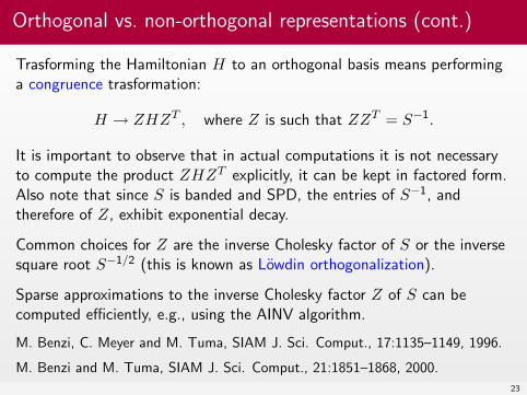
Orthogonal vs. non-orthogonal representations (cont.)

Trasforming the Hamiltonian H to an orthogonal basis means performinga congruence trasformation:

H → ZHZT , where Z is such that ZZT = S−1.

It is important to observe that in actual computations it is not necessaryto compute the product ZHZT explicitly, it can be kept in factored form.Also note that since S is banded and SPD, the entries of S−1, andtherefore of Z, exhibit exponential decay.

Common choices for Z are the inverse Cholesky factor of S or the inversesquare root S−1/2 (this is known as Löwdin orthogonalization).

Sparse approximations to the inverse Cholesky factor Z of S can becomputed efficiently, e.g., using the AINV algorithm.

M. Benzi, C. Meyer and M. T �uma, SIAM J. Sci. Comput., 17:1135–1149, 1996.

M. Benzi and M. T �uma, SIAM J. Sci. Comput., 21:1851–1868, 2000.23

Example: Hamiltonian for C52H106, GTO basis.

24

Example: Hamiltonian for C52H106, orthogonal basis

25

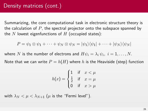
Density matrices (cont.)

Summarizing, the core computational task in electronic structure theory isthe calculation of P , the spectral projector onto the subspace spanned bythe N lowest eigenfunctions of H (occupied states):

P = ψ1 ⊗ ψ1 + · · ·+ ψN ⊗ ψN = |ψ1〉〈ψ1|+ · · ·+ |ψN 〉〈ψN |

where N is the number of electrons and Hψi = λi ψi, i = 1, . . . , N.

Note that we can write P = h(H) where h is the Heaviside (step) function

h(x) =

1 if x < µ12 if x = µ

0 if x > µ

with λN < µ < λN+1 (µ is the “Fermi level”).

26

Outline

1 Motivation


3 Density matrices

4 O(N) methods


27

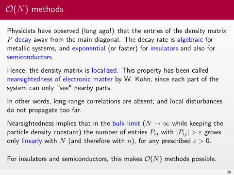
O(N) methods

Physicists have observed (long ago!) that the entries of the density matrixP decay away from the main diagonal. The decay rate is algebraic formetallic systems, and exponential (or faster) for insulators and also forsemiconductors.

Hence, the density matrix is localized. This property has been callednearsightedness of electronic matter by W. Kohn, since each part of thesystem can only “see" nearby parts.

In other words, long-range correlations are absent, and local disturbancesdo not propagate too far.

Nearsightedness implies that in the bulk limit (N →∞ while keeping theparticle density constant) the number of entries Pij with |Pij | > ε growsonly linearly with N (and therefore with n), for any prescribed ε > 0.

For insulators and semiconductors, this makes O(N) methods possible.

28

Example: Density matrix for C52H106, orthogonal basis

29

Example: Plot of |Pij| where P is the density matrix forH = −1

2∆ + V , random V , finite differences (2D lattice),N = 10 occupied states (“Anderson model”).

020

4060

80100

0

20

40

60

80

1000

0.2

0.4

0.6

0.8

1

30

O(N) methods (cont.)

The fact that for many systems of physical interest P is very nearly sparseallows the development of O(N) approximation methods. Some popularmethods are:

1 Chebyshev expansion: P = h(H) ≈ c02 I +

∑nk=1 ckTk(H)

2 Rational expansions based on contour integration:

P =1

2πi

∫Γ(zI −H)−1dz ≈

q∑k=1

wk(zkI −H)−1

3 Density matrix minimization:

Tr(PH) = min, subject to P = P ∗ = P 2 and rank(P ) = N

4 Etc. (see, e.g.: C. Le Bris, Acta Numerica, 2005; Bowler & Miyazaki,Rep. Progr. Phys., 2012)

All these methods can achieve O(N) scaling by exploiting “sparsity.”31

O(N) methods (cont.)

As mentioned, the fact that the density matrix P is exponentially localizedmeans that for any ε > 0, P contains only O(N) elements with |Pij | > ε,as N →∞.

It is possible to show that dropping small entries from P results incontrollable errors in the quantities of interests (e.g., the total energy).

Furthermore, having a priori decay bounds means being able to identifythe positions of the nonnegligible off-diagonal elements of P (“cut-offrules"). Hence, only O(N) elements of P need to be computed.

These two observations are the key to the development of linear scalingmethods.

32

A mathematical foundation for O(N) methods

Until recently, one could not find in the literature any rigorously proved,general results on the decay behavior in P . Decay estimates are eithernon-rigorous (at least for a mathematician!), or valid only for very specialcases. Some physicists even expressed doubts that purely mathematicalarguments could be used to explain nearsightedness!

Using our decay results for matrix functions, one can obtain rigorousestimates for the rate of decay in the off-diagonal entries of P in the formof upper bounds on the entries of the density matrix, uniform in N .

Ideally, these bounds can be used to provide cut-off rules, that is, to decidewhich entries in P need not be computed, given a prescribed errortolerance.

As a result, the possibility of O(N) methods for gapped systems is nowrigorously justified.

33

Intermezzo: two quotes from a physicist...

To obtain a linear scaling, the extended orbitals [i.e., theeigenfunctions of the one-particle Hamiltonian corresponding tooccupied states] have to be replaced by the density matrix,whose physical behavior can be exploited to obtain a fastalgorithm. This last point is essential. Mathematical andnumerical analyses alone are not sufficient to construct a linearalgorithm. They have to be combined with physical intuition.

S. Goedecker, Low complexity algorithms for electronic structure calculations,J. Comp. Phys., 118 (1995), pp. 261–268.

34

Intermezzo: two quotes from a physicist...

Even though O(N) algorithms contain many aspects ofmathematics and computer science they have, nevertheless, deeproots in physics. Linear scaling is not obtainable by purelymathematical tricks, but it is based on an understanding of theconcept of locality in quantum mechanics.

S. Goedecker, Linear scaling electronic structure methods, Rev. Mod. Phys., 71(1999), pp. 1085–1123.

35

... and one from a mathematician

The latter assumption [the exponential localization of the densitymatrix] is in some sense an a posteriori assumption, and not easyto analyse [...] It is to be emphasized that the numerical analysisof the linear scaling methods overviewed above that wouldaccount for cut-off rules and locality assumptions, is not yetavailable.

C. Le Bris, Computational chemistry from the perspective of numerical analysis,Acta Numer., 14 (2005), pp. 363–444.

36

A mathematical foundation for O(N) methods (cont.)

We begin by formalizing the problem at hand.

Let C be a fixed positive integer and let n := C ·N , where N →∞. Wethink of C as the number of basis functions per electron while N is thenumber of electrons.

Definition: A sequence of discrete Hamiltonians is a sequence of n× nHermitian matrices {HN} such that

1 The matrices HN have spectra uniformly bounded w.r.t. N : up toshifting and scaling, we can assume σ(HN ) ⊂ [−1, 1] for all N .

2 The HN are banded, with uniformly bounded bandwidth as N →∞.More generally, the HN are sparse with maximum number ofnonzeros per row bounded w.r.t. N .

These assumptions model the fact that the Hamiltonians have finiteinteraction range.

37

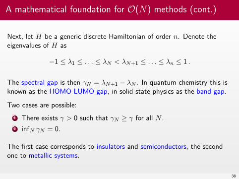
A mathematical foundation for O(N) methods (cont.)

Next, let H be a generic discrete Hamiltonian of order n. Denote theeigenvalues of H as

−1 ≤ λ1 ≤ . . . ≤ λN < λN+1 ≤ . . . ≤ λn ≤ 1 .

The spectral gap is then γN = λN+1 − λN . In quantum chemistry this isknown as the HOMO-LUMO gap, in solid state physics as the band gap.

Two cases are possible:

1 There exists γ > 0 such that γN ≥ γ for all N .2 infN γN = 0.

The first case corresponds to insulators and semiconductors, the secondone to metallic systems.

38

Example: Spectrum of the Hamiltonian for C52H106.

0 100 200 300 400 500 600 700−1.5

−1

−0.5

0

0.5

1

1.5

index i

eig

envalu

es ε

i

ε52

ε53

gap due to core electrons

HOMO−LUMO gapε209

ε210

39

Exponential decay in the density matrix for gapped systems

Our main result is the following

TheoremLet {HN} be a sequence of discrete Hamiltonians of size n = C ·N , withC constant and N →∞. Let PN denote the spectral projector onto theN occupied states associated with HN . If there exists γ > 0 such that thegaps γN ≥ γ for all N , then there exists constants K and α such that

|[PN ]ij | ≤ K e−αdN (i,j) (1 ≤ i, j ≤ N),

where dN (i, j) denotes the distance between node i and node j in thegraph GN associated with HN . The constants K and α depend only onthe gap γ (not on N) and are easily computable, with α = O(γ) as γ → 0.

Note: Explicit expressions for K and α can be found in the cited SIAM Reviewarticle.

40

Exponential decay in the density matrix for gappedsystems (cont.)

Proof (sketch):Recall that the density matrix P can be expressed as P = h(H) whereh(x) is the step function that is equal to 1 on [−1, µ) and equal to 0 on(µ, 1], with µ in the gap between λN and λN+1. If the gap does notvanish as N →∞, then it is is possible to approximate h with anarbitrarily small error on [−1, λN ] and [λN+1, 1] (uniformly in N !) by ananalytic function f(x). Since H has no eigenvalues in the gap, it followsthat ‖P − f(H)‖2 can be made smaller than any prescribed quantity by asuitable choice of f (smooth). The decay results for f(H) then imply thatthe entries in P decay at an exponential (or faster) rate.

Hence, the decay in the density matrix follows from our general theory ofdecay in the entries of analytic functions of sparse matrices.

41

Analytic approximations of the step function

If µ (the “Fermi level”) is in the gap, λN < µ < λN+1, the step functioncan be approximated by the Fermi-Dirac function:

h(x) = limβ→∞

fFD(x), where fFD(x) =1

1 + eβ(x−µ).

Here β can be interpreted as an inverse temperature, β = (κBT )−1.

Other approximations of the step function are also in use, such as

h(x) = limβ→∞

[1

2+

1

πtan−1(βπ(x− µ))

],

h(x) = limβ→∞

erfc (−β(x− µ)) ,

or

h(x) = limβ→∞

[1 + tanh(β((x− µ))] .

42

Co-discoverers of the Fermi–Dirac distribution

Enrico Fermi (1901-1954) and Paul Adrien Maurice Dirac (1902-1984)

43

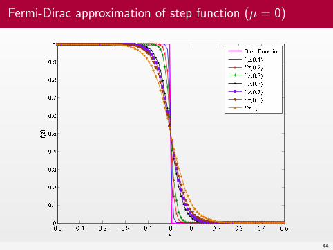
Fermi-Dirac approximation of step function (µ = 0)

44

Fermi-Dirac approximation of step function

The actual choice of β in the Fermi-Dirac function is dictated by the sizeof the gap γ and by the approximation error.

What is important is that for any prescribed error, there is a maximumvalue of β that achieves the error for all N , provided the system hasnon-vanishing gap.

On the other hand, for metallic systems γ → 0, hence β →∞ and thebounds blow up. Indeed, fFD(z) has poles at z = µ± πi/β, hence thedistance from the poles of f to the spectrum tends to zero as β →∞.

There is still decay in the density matrix, but algebraic rather thanexponential. Simple examples show it can be as slow as O(|i− j|−1).

In practice, γ is either known experimentally or can be estimated by computingthe eigenvalues of a moderate-size Hamiltonian.

45

Dependence of decay rate on the spectral gap and on thetemperature

In the physics literature, there has been some controversy on the precisedependence of the inverse correlation length α in the decay estimate

|[PN ]ij | ≤ c · e−α dN (i,j)

on the spectral gap γ (for insulators) and on the electronic temperature T(for metals at positive temperature).

Our theory gives the following results:

1 α = cγ +O(γ3), for γ → 0+ and T = 0;2 α = πκBT +O(T 3), for T → 0+ (indep. of γ).

These asymptotics are in agreement with experimental and numericalresults, as well as with physical intuition.

46

Outline

1 Motivation


3 Density matrices

4 O(N) methods


47

Decay bounds for the Fermi-Dirac approximation

Assume that H is m-banded and has spectrum in [−1, 1], then∣∣∣∣∣[(I + eβ(H−µI)

)−1]

ij

∣∣∣∣∣ ≤ Ke−α|i−j| ≡ K λ|i−j|

m .

Note that K, λ depend only on β. In turn, β depends on γ and on thedesired accuracy.We have

γ → 0+ ⇒ λ→ 1−

andγ → 1 ⇒ λ→ 0.872.

We choose β and m so as to guarantee an error ‖P − fFD(H)‖2 < 10−6.

We can regard γ−1 as a measure of the difficulty of the problem. It is alsoa condition number for the sensitivity of P to perturbations in H.

48

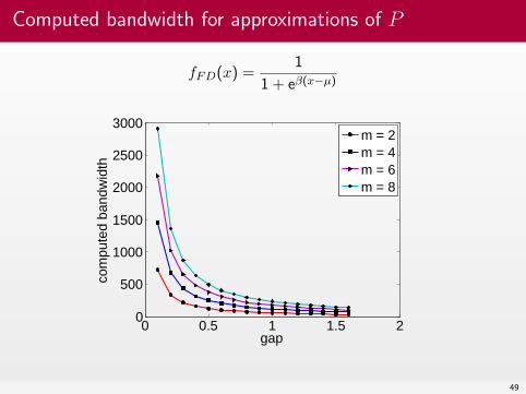
Computed bandwidth for approximations of P

fFD(x) =1

1 + eβ(x−µ)

0 0.5 1 1.5 20

500

1000

1500

2000

2500

3000

gap

com

pute

d ba

ndw

idth

m = 2m = 4m = 6m = 8

49

Approximation of fFD(H) by Chebyshev polynomials

Algorithm (Goedecker & Colombo, 1994) More

We compute approximations of fFD(H) using Chebyshev polynomialsI The degree of the polynomial can be estimated a prioriI The coefficients of the polynomial can be pre-computed (indep. of N)I Estimates for the extreme eigenvalues of H are required

The polynomial expansion is combined with a procedure that a prioridetermines a bandwidth or sparsity pattern for fFD(H) outside whichthe elements are so small that they can be neglected

CostThis method is multiplication-rich; the matrices are kept sparse throughout thecomputation, hence O(N) arithmetic and storage requirements. The matrixpolynomials can be efficiently evaluated by the Paterson-Stockmeyer algorithm.

50

Chebyshev expansion of Fermi-Dirac function

The bandwidth was computed prior to the calculation to be ≈ 20; here His tridiagonal (toy example).

Table: Results for fFD(x) = 11+e(β(x−µ))

µ = 2, β = 2.13 µ = 0.5, β = 1.84

N error k m error k m

100 9e−06 18 20 6e−06 18 22

200 4e−06 19 20 9e−06 18 22

300 4e−06 19 20 5e−06 20 22

400 6e−06 19 20 8e−06 20 22

500 8e−06 19 20 8e−06 20 22

Note: In the table, ‘error’ means relative error in the Frobenius norm.

51

Computation of Fermi-Dirac function

100 150 200 250 300 350 400 450 5000.5

1

1.5

2

2.5

3

3.5x 10

6

n

# of

ope

ratio

ns

mu = 2, beta = 2.13mu = 0.5, beta = 2.84

The O(N) behavior of Chebyshev’s approximation to the Fermi–Diracfunction fFD(H) = (exp(β(H − µI)) + I)−1.

52

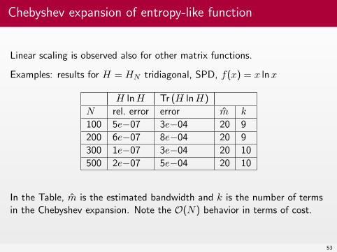
Chebyshev expansion of entropy-like function

Linear scaling is observed also for other matrix functions.

Examples: results for H = HN tridiagonal, SPD, f(x) = x lnx

H lnH Tr (H lnH)

N rel. error error m k

100 5e−07 3e−04 20 9

200 6e−07 8e−04 20 9

300 1e−07 3e−04 20 10

500 2e−07 5e−04 20 10

In the Table, m is the estimated bandwidth and k is the number of termsin the Chebyshev expansion. Note the O(N) behavior in terms of cost.

53

Summary

‘Gapped’ systems, like insulators, exhibit strong localizationLocalization in P = h(H), when present, can lead to fastapproximation algorithmsOur decay bounds for density matrices depend only on the gap γ andon the sparsity of H; they are, in a sense, universalThese bounds can be useful in determining appropriate sparsitypatterns (or bandwidths) that capture the nonnegligible entries inP = h(H)

Constants in O(N) algorithms can be large. In practice, to beatsub-optimal, O(Np) algorithms (p = 2, 3) algorithms N must bequite large.

54

Chebyshev approximation

For H with σ(H) ⊂ [−1, 1] the Chebyshev polynomials are given by

Tk+1(H) = 2HTk(H)− Tk−1(H), T1(H) = H, T0(H) = I.

Then f(H) can be represented in a series of the form

f(H) =∞∑

k=0

ckTk(H).

The coefficients of the expansion are given by

ck ≈2

M

M∑j=1

f(cos(θj)) cos((k − 1)θj),

where θj = π(j − 12)/M . Back

55

The N -independence of the error

The mth truncation error without dropping can be written as

‖em(H)‖ = ‖f(H)−m∑

k=0

ckTk(H)‖.

For x in [−1, 1] we have that |Tk(x)| ≤ 1 for k = 1, 2, . . . . Then

‖em(H)‖ = ‖∞∑

k=m+1

ckTk(H)‖ ≤∞∑

k=m+1

|ck|.

Back

56

lecture v: matrix functions in quantum chemistrybenzi/web_papers/dob5.pdf · dobbiaco, 15-20 june,...

Documents