lecture on sections 1.3,1 - university of kentucky
TRANSCRIPT

Lecture on sections 1.3,1.4
Ma 162 Spring 2010
Ma 162 Fall 2010
August 30, 2010
Avinash Sathaye (Ma 162 Fall 2010) Continued Coordinate Geometry August 30, 2010 1 / 15

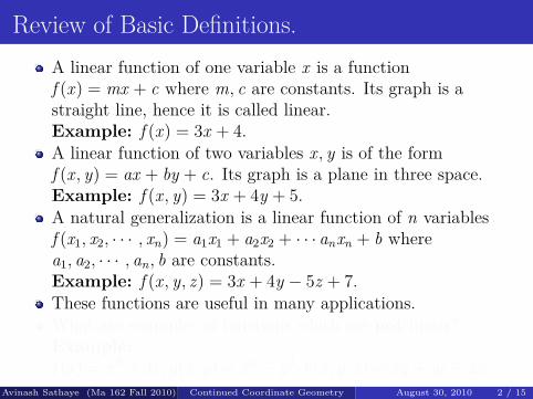
Review of Basic Definitions.A linear function of one variable x is a functionf (x) = mx + c where m, c are constants. Its graph is astraight line, hence it is called linear.Example: f (x) = 3x + 4.A linear function of two variables x , y is of the formf (x , y) = ax + by + c. Its graph is a plane in three space.Example: f (x , y) = 3x + 4y + 5.A natural generalization is a linear function of n variablesf (x1, x2, · · · , xn) = a1x1 + a2x2 + · · · anxn + b wherea1, a2, · · · , an, b are constants.Example: f (x , y, z) = 3x + 4y − 5z + 7.These functions are useful in many applications.What are examples of functions which are not linear?Example:f (x) = x2 + 3x , g(x , y) = x3 − y3, h(x , y, z) = xy + yz + zx .
Avinash Sathaye (Ma 162 Fall 2010) Continued Coordinate Geometry August 30, 2010 2 / 15

Some interesting Linear Functions
Here are some examples of real life functions which behave likelinear functions.
Tax Calculations. Typically, tax calculation on an incomeof x dollars is a linear function when x lies in a specific taxbracket. The function formula, however, changes with taxbrackets. This is a good example of a step function which isdefined by different formulas in different ranges of x values.A typical formula looks like
t(x) = f + r(x − b)
where x is assumed to be at least b, f is the fixed tax forincome b and r is the tax on each dollar earned above b.
Avinash Sathaye (Ma 162 Fall 2010) Continued Coordinate Geometry August 30, 2010 3 / 15

Tax Calculations continued.
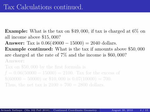
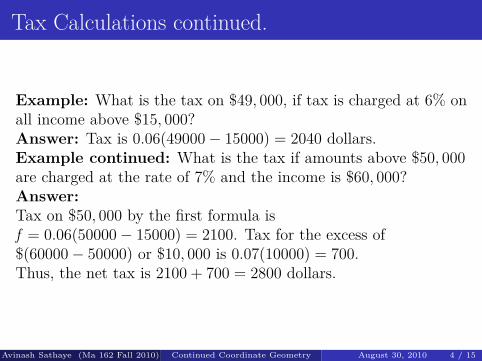
Example: What is the tax on $49, 000, if tax is charged at 6% onall income above $15, 000?Answer: Tax is 0.06(49000 − 15000) = 2040 dollars.Example continued: What is the tax if amounts above $50, 000are charged at the rate of 7% and the income is $60, 000?Answer:Tax on $50, 000 by the first formula isf = 0.06(50000 − 15000) = 2100. Tax for the excess of$(60000 − 50000) or $10, 000 is 0.07(10000) = 700.Thus, the net tax is 2100 + 700 = 2800 dollars.
Avinash Sathaye (Ma 162 Fall 2010) Continued Coordinate Geometry August 30, 2010 4 / 15
Tax Calculations continued.
Example: What is the tax on $49, 000, if tax is charged at 6% onall income above $15, 000?Answer: Tax is 0.06(49000 − 15000) = 2040 dollars.Example continued: What is the tax if amounts above $50, 000are charged at the rate of 7% and the income is $60, 000?Answer:Tax on $50, 000 by the first formula isf = 0.06(50000 − 15000) = 2100. Tax for the excess of$(60000 − 50000) or $10, 000 is 0.07(10000) = 700.Thus, the net tax is 2100 + 700 = 2800 dollars.
Avinash Sathaye (Ma 162 Fall 2010) Continued Coordinate Geometry August 30, 2010 4 / 15

Depreciation.
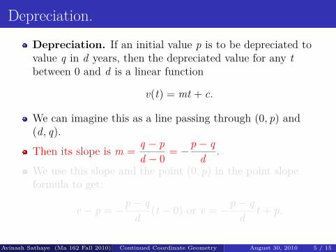
Depreciation. If an initial value p is to be depreciated tovalue q in d years, then the depreciated value for any tbetween 0 and d is a linear function
v(t) = mt + c.
We can imagine this as a line passing through (0, p) and(d, q).
Then its slope is m = q − pd − 0 = −p − q
d .
We use this slope and the point (0, p) in the point slopeformula to get:
v − p = −p − qd (t − 0) or v = −p − q
d t + p.
Avinash Sathaye (Ma 162 Fall 2010) Continued Coordinate Geometry August 30, 2010 5 / 15

Depreciation.
Depreciation. If an initial value p is to be depreciated tovalue q in d years, then the depreciated value for any tbetween 0 and d is a linear function
v(t) = mt + c.
We can imagine this as a line passing through (0, p) and(d, q).
Then its slope is m = q − pd − 0 = −p − q
d .
We use this slope and the point (0, p) in the point slopeformula to get:
v − p = −p − qd (t − 0) or v = −p − q
d t + p.
Avinash Sathaye (Ma 162 Fall 2010) Continued Coordinate Geometry August 30, 2010 5 / 15
Example of depreciation.
Example: If a car worth $45, 000 is to be depreciated to zeroin 6 years, what is its value after 4 years.We have p = 45, 000, q = 0 and d = 6. Thus the formula is
v = −450006 t + 45000 so at t = 4 we get − 45000
6 4 + 45000.
This gives v = 15000 as the answer.
Avinash Sathaye (Ma 162 Fall 2010) Continued Coordinate Geometry August 30, 2010 6 / 15

Financial Functions
Review of Business Functions. If x is the number ofunits sold or manufactured, then we have three naturalfunctions associated with it.The cost function is C (x) = cx + f where c is the productioncost per unit and f is the fixed cost.The revenue function is R(x) = px where p is the selling priceof a unit.The profit function is then given byP(x) = R(x) − C (x) = (p − c)x − f .
Avinash Sathaye (Ma 162 Fall 2010) Continued Coordinate Geometry August 30, 2010 7 / 15
Break even Analysis
We now describe how to determine the minimum production levelwhich guarantees no net loss.
Break even Production. A production level x is said to bebreak even if the net profit is zero, i.e.
P(x) = R(x) − C (x) = (p − c)x − f = 0.
Another viewpoint. The break even production can beinterpreted alternatively as follows.Consider the graphs of the revenue function R(x) and thecost function C (x) plotted on the same axes. Both graphs arelines.Then the break even production is simply the x-coordinate ofthe common point.
Avinash Sathaye (Ma 162 Fall 2010) Continued Coordinate Geometry August 30, 2010 8 / 15

Example of Break even Analysis.
Example. Suppose that a certain toy can be manufactured for$3.5 each and the cost of maintaining the workshop is $21, 000 permonth.If the toy is sold for $5, determine the monthly break evenproduction.Answer: Let x denote the monthly production. Then the revenuefunction is R(x) = 5x . The cost function is C (x) = 3.5x + 21000.We find the common point of the graphs of y = R(x) andy = C (x), thus we solve:
5x = 3.5x + 21000 or 1.5x = 21000.
The break even production is x = 210001.5 = 14000.
Avinash Sathaye (Ma 162 Fall 2010) Continued Coordinate Geometry August 30, 2010 9 / 15

Intersecting lines
The above example motivates a review of techniques to intersecttwo lines.We consider two linear equations ax + by = c and px + qy = r anddiscuss their common solutions.
Substitution method. The most familiar method is tosolve one of the equations for y and substitute the solution inthe other to find the x-coordinate of the common point.Then use it and one of the equations to find y. Example:Solve
E1 : 3x − y = 5 and E2 : 2x + 3y = 7.
Answer: Solving E1 for y, we get y = 3x − 5. Substitutionin E2 gives: 2x + 3(3x − 5) = 7 or 11x = 22. This gives x = 2and finally y = 3x − 5 = 3(2) − 5 = 1.
Avinash Sathaye (Ma 162 Fall 2010) Continued Coordinate Geometry August 30, 2010 10 / 15

Continued Intersections of Lines.
Thus, the intersection of the lines
E1 : 3x − y = 5 and E2 : 2x + 3y = 7
is given by x = 2, y = 1.Comment. Though easy to understand, the above methodis not always the most efficient and it is helpful to learn othertechniques as well.Cramer’s Rule. This technique lets us write down theanswer to a system of two linear equations in two variablesby a formula.It can also generalize to several equations in several variables.
Avinash Sathaye (Ma 162 Fall 2010) Continued Coordinate Geometry August 30, 2010 11 / 15

Determinants.
Determinant. Given a 2 × 2 matrix A =[
a bc d
]we define
its determinant:det(A) = ad − bc.
Sometimes this is also written as∣∣∣∣∣ a bc d
∣∣∣∣∣ = ad − bc.
Example: ∣∣∣∣∣ 5 −32 4
∣∣∣∣∣ = (5)(4) − (−3)(2) = 26.
Avinash Sathaye (Ma 162 Fall 2010) Continued Coordinate Geometry August 30, 2010 12 / 15

Cramer’s Rule.
Now we describe the Cramer’s rule for solving two equationsin two variables:
E1 : ax + by = c, E2 : px + qy = r .
Calculate the determinants:
∆ =∣∣∣∣∣ a b
p q
∣∣∣∣∣ , ∆x =∣∣∣∣∣ c b
r q
∣∣∣∣∣ , ∆y =∣∣∣∣∣ a c
p r
∣∣∣∣∣ .Then the answers are:
x = ∆x
∆ and y = ∆y
∆ .
Avinash Sathaye (Ma 162 Fall 2010) Continued Coordinate Geometry August 30, 2010 13 / 15
Cramer’s Rule: continued.
Recall the answers:
x = ∆x
∆ and y = ∆y
∆ .
These are undefined when ∆ = 0 and in that case we have:If one of ∆x , ∆y is non zero, then the system has no solution.If all three determinants are zero then one equation is amultiple of another and we could have infinitely manysolutions unless we happen to have an equation where allcoefficients of variables are zero and some right hand side isnon zero!
Avinash Sathaye (Ma 162 Fall 2010) Continued Coordinate Geometry August 30, 2010 14 / 15
Example of Cramer’s Rule.We redo the old example.Example: Solve
E1 : 3x − y = 5 and E2 : 2x + 3y = 7.
Answer: We see that
∆ =∣∣∣∣∣ 3 −12 3
∣∣∣∣∣ , ∆x =∣∣∣∣∣ 5 −17 3
∣∣∣∣∣ , ∆y =∣∣∣∣∣ 3 52 7
∣∣∣∣∣ .Evaluation gives:
∆ = (3)(3) − (−1)(2) = 11∆x = (5)(3) − (−1)(7) = 22∆y = (3)(7) − (5)(2) = 11
So the answers are:
x = 2211 = 2, y = 11
11 = 1
as already known!Avinash Sathaye (Ma 162 Fall 2010) Continued Coordinate Geometry August 30, 2010 15 / 15