Lecture notes to Stock and Watson chapter 11Probit and logit regression

Tore Schweder

October 2008

TS () LN10 13/10 1 / 17

Outline

Review of estimator consistency

Review: the panel data regression study of drunk driving in the USA

Binary regression - why?

Probit and logit - cases of the generalized linear model, glm

Maximum likelihood estimation

Application to Boston Home Mortgage Data: is there a race bias inmortgage denials?

TS () LN10 13/10 2 / 17

Consistency

An estimator bθ is consistent whenever bθ P! θ, i.eP�jbθ � θj > ε

�! 0 for all ε > 0, as the data increases to ∞.

Consistency means that the probability distribution of bθ gets moreand more concentrated around the "true" value of the parameter.

Exercise SW: 10.10!

TS () LN10 13/10 3 / 17

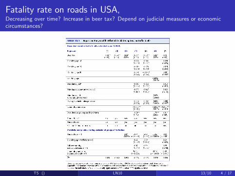
Fatality rate on roads in USA,Decreasing over time? Increase in beer tax? Depend on judicial measures or economiccircumstances?

TS () LN10 13/10 4 / 17

Fatality rate on roads in USADecreases over time!

How can the fatality rate decrease with unemployment rate, andincrease with income?

TS () LN10 13/10 5 / 17

Regression for binary response variablesExample questions

1 Is the probability of a bank going bust during 2008 dependent onstate regulations?

Frame: banks registered 1. January 2008 in OECD countriesExplanatory variable: dummies for regulations of various types (requiredcapital basis; investment bank ok; insurance ok; savings secured;...)Control variables: Size of bank (turnover; employed;...); Ownership;...Response variable: binary Yes/NoIs there room for a �xed e¤ect of country?What about external validity of such regression results?

2 Can the probability of the baby being boy be manipulated?Frame: Norwegian live births in 2007Explanatory variables: Age of mother and father; pattern of sexualintercourse (frequency);...Response variable: boy/girl

3 Is the probability of soccer club i winning over club j dependentadditively on club-speci�c �xed e¤ect parameters, i.e. on βi � βj ?

TS () LN10 13/10 6 / 17

Example: Mortgage denials in Boston

TS () LN10 13/10 7 / 17

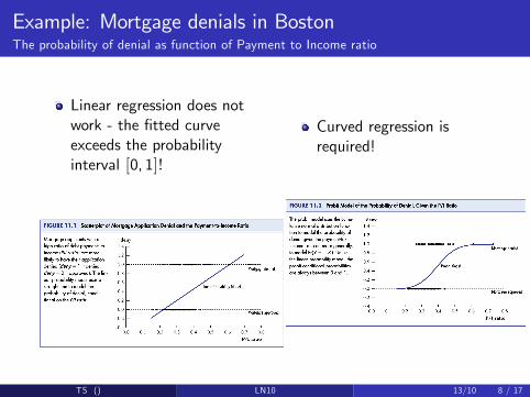
Example: Mortgage denials in BostonThe probability of denial as function of Payment to Income ratio

Linear regression does notwork - the �tted curveexceeds the probabilityinterval [0, 1]!

Curved regression isrequired!

TS () LN10 13/10 8 / 17

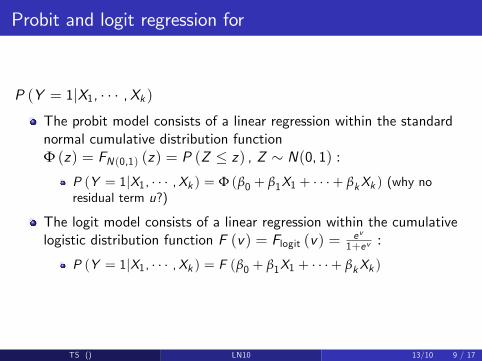
Probit and logit regression for

P (Y = 1jX1, � � � ,Xk )The probit model consists of a linear regression within the standardnormal cumulative distribution functionΦ (z) = FN (0,1) (z) = P (Z � z) , Z � N(0, 1) :

P (Y = 1jX1, � � � ,Xk ) = Φ (β0 + β1X1 + � � �+ βkXk ) (why noresidual term u?)

The logit model consists of a linear regression within the cumulativelogistic distribution function F (v) = Flogit (v) = ev

1+ev :

P (Y = 1jX1, � � � ,Xk ) = F (β0 + β1X1 + � � �+ βkXk )

TS () LN10 13/10 9 / 17

Comparing the standard normal (probit) and the logistic(logit) curves

z

cdf

­4 ­2 0 2 4

0.0

0.2

0.4

0.6

0.8

1.0

normallogistic

z

v

­4 ­2 0 2 4

­10

­50

510

QQ logistic vs normalv = 1.88z

v

cdf

­4 ­2 0 2 4

0.0

0.2

0.4

0.6

0.8

1.0

scaled normallogistic

Figure: UL: The cumulative distribution functions (cdf) Φ and Flogit; UR:

QQ-plot of the logistic versus the normal distribution,�

Φ�1 (p) ,F�1logit (p)�

0 < p < 1, the logistic has fatter tails than the normal!; LR: The scaled normalΦ (v/1.88) and Flogit (v)

TS () LN10 13/10 10 / 17

Maximum likelihood estimationLogistic regression

pi = p (Xi1, � � � ,Xk ) = Flogit (Xi1, � � � ,Xik ) is the conditional "success"probability (denial of mortgage) for unit i

For y = 1 and y = 0

P (Yi = y jXi1, � � � ,Xik ) = pyi (1� pi )1�y

By independence across units, the conditional joint outcomeprobability is

P (Y1 = y1, � � � ,Yn = yn) =n

∏i=1pyi (1� pi )

1�y = L (β0, β1, � � � , βk )

L (β0, β1, � � � , βk ) is the likelihood function - for observed data it is afunction of the parameters

The (joint) maximum likelihood estimator�bβ0, bβ1, � � � , bβk�

maximizes L (β0, β1, � � � , βk )TS () LN10 13/10 11 / 17

A simple example of logistic regressionmaximum likelihood estimation

Model: P(Y = 1jx) = FLogit (βx) no intercept. True value: β = 0.5,x= -5 -4 -3 -2 -1 0 1 2 3 4 5

beta

log.

likel

ihoo

d

­0 .5 0.0 0.5 1.0 1.5

­12

­11

­10

­9­8

Y = 10001001110

beta

log.

likel

ihoo

d

­0 .5 0.0 0.5 1.0 1.5

­10

­9­8

­7­6

­5

Y = 00001100111

beta

log.

likel

ihoo

d

­0 .5 0.0 0.5 1.0 1.5

­11

­10

­9­8

­7­6

Y = 00000001110

beta

log.

likel

ihoo

d

­0 .5 0.0 0.5 1.0 1.5

­11

­10

­9­8

­7­6

Y = 10000001111

Figure: Log likelihood log(L) for four di¤erent realizations of (Y�5, � � � ,Y5)shown in the panel titel.TS () LN10 13/10 12 / 17

Mortgage denials in Boston, logit and probit regressions

TS () LN10 13/10 13 / 17

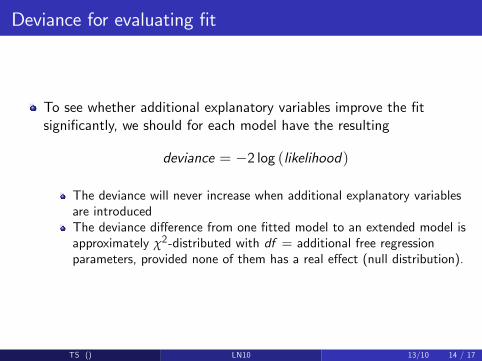
Deviance for evaluating �t

To see whether additional explanatory variables improve the �tsigni�cantly, we should for each model have the resulting

deviance = �2 log (likelihood)

The deviance will never increase when additional explanatory variablesare introducedThe deviance di¤erence from one �tted model to an extended model isapproximately χ2-distributed with df = additional free regressionparameters, provided none of them has a real e¤ect (null distribution).

TS () LN10 13/10 14 / 17

Mortgage denials in BostonAre black applicants discriminated?

The interactions in model 6 makes interpretation more involved

Recalling that logit regression parameters are about 1.88 as large asprobit regression parameters, models 2-5 give roughly the sameanswer: the probit estimate for black is about 0.38.

Everything else equal, the di¤erence in predicted (�tted) value on theprobit scale for a black applicant is moved 0.38 units to the rightrelative to that for a white applicants.In terms of probability of denial, the di¤erence depend on where on thescale the two points are. If the two applicants have average values onall other variables, the black has 6-7 percentage points higherprobability of being denied.

TS () LN10 13/10 15 / 17

Logistic regression is easier to interpret!

Let pblack and pwhite be the denial probabilities for the black and the whiteapplicant that otherwise are identical. In logistic regression the log odds isfor the black person

log (Oblack ) = log�

pblack1� pblack

�= βblack +∑

jβjXj

where the sum is over all other regressors including the intercept.The log odds for the white person is

log (Owhite ) = log�

pwhite1� pwhite

�= ∑

jβjXj .

The log odds ratio is thus

log�OblackOwhite

�= log (Oblack )� log (Owhite ) = βblack

Regardless of the other explanatory variables for the two otherwise identicalblack and white, the log odds ratio is 0.7 for black versus white (model 2).

TS () LN10 13/10 16 / 17

Summing up

OLS is stupid when the response variable is dichotomous (a dummy)

Use probit or logit regression! Probit is fashionable in econometrics,but logistic regression is slightly preferable for statistical andinterpretational reasons

Probit regression and logit regression are cases of the generalizedlinear model (glm) with Bernoulli (binomial) variational model andwith the probit or logit link function mapping the linear predictor tothe expected response: E (Y ) = FLogit

�∑j βjXj

�etc. See SW:

Appendix 11.3, andhttp://en.wikipedia.org/wiki/Generalized_linear_model

Individual coe¢ cients can be tested by t-test. To test whether someparameters are all zero, compare the deviance di¤erence to theappropriate χ2-distribution.

Do SW: 11.6

TS () LN10 13/10 17 / 17