lecture notes subject code: cs2352 subject name
TRANSCRIPT

www.vidyarthiplus.com
www.vidyarthiplus.com Page 1
LECTURE NOTES
Subject Code: CS2352
Subject Name: PRINCIPLES OF COMPILER DESIGN

UNIT I - INTRODUCTION TO COMPILING- LEXICAL ANALYSIS
COMPILERS
A compiler is a program that reads a program in one language, the source language and
translates into an equivalent program in another language, the target language.The translation
process should also report the presence of errors in the source program.
Source
Program → Compiler →
Target
Target
Program
↓
Error
Messages ANALYSIS OF THE SOURCE PROGRAM
There are two parts of compilation.
Analysis part
Synthesis Part
The analysis part breaks up the source program into constant piece and creates an
intermediate representation of the source program.
The synthesis part constructs the desired target program from the intermediate
representation. Analysis consists of three phases:
Linear analysis (Lexical analysis or Scanning)) :
The lexical analysis phase reads the characters in the source program and grouped into
them tokens that are sequence of characters having a collective meaning.
Example : position : = initial + rate * 60
Identifiers – position, initial, rate.
Assignment symbol - : =
Operators - + , *
Number - 60
Blanks – eliminated.
Hierarchical analysis (Syntax analysis or Parsing) :
It involves grouping the tokens of the source program into grammatical phrases that are
used by the complier to synthesize output.

Example : position : = initial + rate * 60
Semantic analysis :
In this phase checks the source program for semantic errors and gathers type
information for subsequent code generation phase.
An important component of semantic analysis is type checking.
Example : int to real conversion.
PHASES OF COMPILER The compiler has a number of phases plus symbol table manager and an error handler.
The first three phases, forms the bulk of the analysis portion of a compiler. Symbol table
management and error handling, are shown interacting with the six phases.
Symbol table management
An essential function of a compiler is to record the identifiers used in the source program
and collect information about various attributes of each identifier. A symbol table is a data
structure containing a record for each identifier, with fields for the attributes of the identifier.
The data structure allows us to find the record for each identifier quickly and to store or retrieve
data from that record quickly. When an identifier in the source program is detected by the lex
analyzer, the identifier is entered into the symbol table.
Error Detection and Reporting
Each phase can encounter errors. A compiler that stops when it finds the first error is not
as helpful as it could be.The syntax and semantic analysis phases usually handle a large fraction
of the errors detectable by the compiler. The lexical phase can detect errors where the characters
remaining in the input do not form any token of the language. Errors when the token stream
violates the syntax of the language are determined by the syntax analysis phase. During semantic
analysis the compiler tries to detect constructs that have the right syntactic structure but no
meaning to the operation involved. The Analysis phases
As translation progresses, the compiler’s internal representation of the source program
changes. Consider the statement, position := initial + rate * 10
The lexical analysis phase reads the characters in the source pgm and groups them into a
stream of tokens in which each token represents a logically cohesive sequence of characters,
such as an identifier, a keyword etc. The character sequence forming a token is called the lexeme
for the token. Certain tokens will be augmented by a ‘lexical value’. For example, for any
identifier the lex analyzer generates not only the token id but also enter s the lexeme into the
symbol table, if it is not already present there. The lexical value associated this occurrence of id
points to the symbol table entry for this lexeme. The representation of the statement given above
after the lexical analysis would be: id1: = id2 + id3 * 10
Syntax analysis imposes a hierarchical structure on the token stream, which is shown by syntax
trees Intermediate Code Generation
After syntax and semantic analysis, some compilers generate an explicit intermediate
representation of the source program. This intermediate representation can have a variety of
forms.In three-address code, the source pgm might look like this, temp1: = inttoreal (10)
temp2: = id3 * temp1
temp3: = id2 + temp2
id1: = temp3
Code Optimisation
The code optimization phase attempts to improve the intermediate code, so that faster
running machine codes will result. Some optimizations are trivial. There is a great variation in
the amount of code optimization different compilers perform. In those that do the most, called
‘optimising compilers’, a significant fraction of the time of the compiler is spent on this phase.
Code Generation
The final phase of the compiler is the generation of target code, consisting normally of
relocatable machine code or assembly code. Memory locations are selected for each of the
variables used by the program. Then, intermediate instructions are each translated into a
sequence of machine instructions that perform the same task. A crucial aspect is the assignment
of variables to registers. COUSINS OF THE COMPILER
Cousins of the Complier (Language Processing System) :
Preprocessors : It produces input to Compiler. They may perform the following functions.
Macro Processing : A preprocessor may allow a user to define macros that are shorthands for longer constructs.
File inclusion : A preprocessor may include header files into the program text.
Rational preprocessors : These preprocessors augment older language with more modern flow of control and data
structuring facilities.
Language extensions : These preprocessor attempt to add capabilities to the language by what amounts to built in
macros.
Complier : It converts the source program(HLL) into target program (LLL).
Assembler : It converts an assembly language (LLL) into machine code.
Loader and Link Editors :
Loader : The process of loading consists of taking relocatable machine code, altering the relocatable
addresses and placing the altered instructions and data in memory at the proper locations.
Link Editor : It allows us to make a single program from several files of relocatable machine code.

GROUPING OF PHASES
Classification of Compiler :
1. Single Pass Complier
2. Multi-Pass Complier
3. Load and Go Complier
4. Debugging or Optimizing Complier. Software Tools : Many software tools that manipulate source programs first perform some kind of analysis. Some
examples of such tools include:
Structure Editors : A structure editor takes as input a sequence of commands to build a source program.
The structure editor not only performs the text-creation and modification functions of an
ordinary text editor, but it also analyzes the program text, putting an appropriate hierarchical
structure on the source program.
Example – while …. do and begin….. end.
Pretty printers : A pretty printer analyzes a program and prints it in such a way that the structure of the
program becomes clearly visible.
Static Checkers : A static checker reads a program, analyzes it, and attempts to discover potential bugs
without running the program.
Interpreters : Translate from high level language ( BASIC, FORTRAN, etc..) into assembly or machine
language. Interpreters are frequently used to execute command language, since each operator
executed in a command language is usually an invocation of a complex routine such as an editor
or complier.The analysis portion in each of the following examples is similar to that of a
conventional complier.
Text formatters.
Silicon Compiler.
Query interpreters.
COMPILER CONSTRUCTION TOOLS
Parser Generators: The specification of input based on regular expression. The organization is based on finite
automation.
Scanner Generator: The specification of input based on regular expression. The organization is based on finite
automation.

Syntax-Directed Translation:
It walks the parse tee and as a result generate intermediate code.
Automatic Code Generators: Translates intermediate rampage into machine language.
Data-Flow Engines: It does code optimization using data-flow analysis.
LEXICAL ANALYSIS
A simple way to build lexical analyzer is to construct a diagram that illustrates the
structure of the tokens of the source language, and then to hand-translate the diagram into a
program for finding tokens. Efficient lexical analysers can be produced in this manner. ROLE OF LEXICAL ANALYSER
The lexical analyzer is the first phase of compiler. Its main task is to read the input
characters and produces output a sequence of tokens that the parser uses for syntax analysis. As
in the figure, upon receiving a “get next token” command from the parser the lexical analyzer
reads input characters until it can identify the next token.
Since the lexical analyzer is the part of the compiler that reads the source text, it may also
perform certain secondary tasks at the user interface. One such task is stripping out from the
source program comments and white space in the form of blank, tab, and new line character.
Another is correlating error messages from the compiler with the source program. Issues in Lexical Analysis
There are several reasons for separating the analysis phase of compiling into lexical analysis and
parsing.

1) Simpler design is the most important consideration. The separation of lexical analysis from
syntax analysis often allows us to simplify one or the other of these phases.
2) Compiler efficiency is improved.
3) Compiler portability is enhanced.
Tokens Patterns and Lexemes.
There is a set of strings in the input for which the same token is produced as output. This
set of strings is described by a rule called a pattern associated with the token. The pattern is set to
match each string in the set. A lexeme is a sequence of characters in the source program that is
matched by the pattern for the token. For example in the Pascal’s statement const pi = 3.1416;
the substring pi is a lexeme for the token identifier.
In most programming languages, the following constructs are treated as tokens:
keywords, operators, identifiers, constants, literal strings, and punctuation symbols such as
parentheses, commas, and semicolons.
TOKEN SAMPLE LEXEMES INFORMAL DESCRIPTION OF PATTERN
const
if
relation
id
num
literal
Const
if
<,<=,=,<>,>,>=
pi,count,D2
3.1416,0,6.02E23
“core dumped”
const
if
< or <= or = or <> or >= or >
letter followed by letters and digits
any numeric constant
any characters between “ and “ except”
A pattern is a rule describing a set of lexemes that can represent a particular token in
source program. The pattern for the token const in the above table is just the single string const
that spells out the keyword.
Certain language conventions impact the difficulty of lexical analysis. Languages such as
FORTRAN require a certain constructs in fixed positions on the input line. Thus the alignment of
a lexeme may be important in determining the correctness of a source program.
Attributes of Token

The lexical analyzer returns to the parser a representation for the token it has found. The
representation is an integer code if the token is a simple construct such as a left parenthesis,
comma, or colon .The representation is a pair consisting of an integer code and a pointer to a
table if the token is a more complex element such as an identifier or constant .The integer code
gives the token type, the pointer points to the value of that token .Pairs are also retuned whenever
we wish to distinguish between instances of a token. INPUT BUFFERING
The lexical analyzer scans the characters of the source program one a t a time to discover
tokens. Often, however, many characters beyond the next token many have to be examined
before the next token itself can be determined. For this and other reasons, it is desirable for the
lexical analyzer to read its input from an input buffer. Figure shows a buffer divided into two
haves of, say 100 characters each. One pointer marks the beginning of the token being
discovered. A look ahead pointer scans ahead of the beginning point, until the token is
discovered .we view the position of each pointer as being between the character last read and the
character next to be read. In practice each buffering scheme adopts one convention either a
pointer is at the symbol last read or the symbol it is ready to read.
Token beginnings look ahead pointer
The distance which the lookahead pointer may have to travel past the actual token may be
large. For example, in a PL/I program we may see:
DECALRE (ARG1, ARG2… ARG n)
Without knowing whether DECLARE is a keyword or an array name until we see the
character that follows the right parenthesis. In either case, the token itself ends at the second E.
If the look ahead pointer travels beyond the buffer half in which it began, the other half must be
loaded with the next characters from the source file.
Since the buffer shown in above figure is of limited size there is an implied constraint on
how much look ahead can be used before the next token is discovered. In the above example, if
the look ahead traveled to the left half and all the way through the left half to the middle, we
could not reload the right half, because we would lose characters that had not yet been grouped
into tokens. While we can make the buffer larger if we chose or use another buffering scheme,
we cannot ignore the fact that overhead is limited.

SPECIFICATION OF TOKENS Strings and Languages
The term alphabet or character class denotes any finite set of symbols. Typically
examples of symbols are letters and characters. The set {0, 1} is the binary alphabet.
A String over some alphabet is a finite sequence of symbols drawn from that alphabet. In
Language theory, the terms sentence and word are often used as synonyms for the term “string”.
The term language denotes any set of strings over some fixed alphabet. This definition is
very broad. Abstract languages like the empty set, or { t he set containing only the empty
set, are languages under this definition.
Certain terms fro parts of a string are prefix, suffix, substring, or subsequence of a string.
There are several important operations like union, concatenation and closure that can be applied
to languages.
Regular Expressions
In Pascal, an identifier is a letter followed by zero or more letters or digits. Regular
expressions allow us to define precisely sets such as this. With this notation, Pascal identifiers
may be defined as
letter (letter | digit)* The vertical bar here means “or” , the parentheses are used to group subexpressions, the star
means “ zero or more instances of” the parenthesized expression, and the juxtaposition of letter
with remainder of the expression means concatenation.
A regular expression is built up out of simpler regular expressions using set of defining
rules. Each regular expression r denotes a language L(r). The defining rules specify how L(r) is
formed by combining in various ways the languages denoted by the subexpressions of r. Unnecessary parenthesis can be avoided in regular expressions if we adopt the conventions that:
1. the unary operator has the highest precedence and is left associative.
2. concatenation has the second highest precedence and is left associative. 3. | has the lowest precedence and is left associative.

Regular Definitions
If i s an alphabet of basic symbols, then a regular definition is a sequence of definitions
of the form d r , d’ r’ where d,d’ is a distinct name , and
, d’ r’ where d,d’ is a distinct name , and
r,r’ is a regular expression over
r,r’ is a regular expression over
the symbols i {d,d’,…} , i.e.; the basic symbols and the previously defined names.
Example: The set of Pascal identifiers is the set of strings of letters and digits beginning with a
letter. The regular definition for the set is
letter A|B|…|Z|a|b|…z
digit
id letter ( letter | digit ) *
Unsigned numbers in Pascal are strings such as 5280,56.77,6.25E4 etc. The following
regular definition provides a precise specification for this class of strings:
digit
digits igit digit *
This definition says that digit can be any number from 0-9, while digits is a digit
followed by zero or more occurrences of a digit.
Notational Shorthands
Certain constructs occur so frequently in regular expressions that it is convenient to introduce
notational shorthands for them.
1. One or more instances. The unary postfix operator + means “one or more instances of
“
2. Zero or one instance. The unary postfix operator ? means “zero or one instance of “.
The notation r? is a shorthand
3. Character classes. The notation [abc] where a , b , and c are the alphabet symbols
denotes the regular expression a|b|c. An abbreviated character class such as [a-z]
denotes the regular expression a|b|c|……….|z.

UNIT II - SYNTAX ANALYSIS AND RUNTIME ENVIRONMENT
ROLE OF THE PARSER
Parser obtains a string of tokens from the lexical analyzer and verifies that it can be generated
by the language for the source program. The parser should report any syntax errors in an
intelligible fashion. The two types of parsers employed are:
1.Top down parser: which build parse trees from top(root) to bottom(leaves)
2.Bottom up parser: which build parse trees from leaves and work up the root. Therefore there are two types of parsing methods– top-down parsing and bottom-up parsing
WRITING GRAMMARS
A grammar consists of a number of productions. Each production has an abstract symbol
called a nonterminal as its left-hand side, and a sequence of one or more nonterminal and
terminal symbols as its right-hand side. For each grammar, the terminal symbols are drawn from
a specified alphabet.
Starting from a sentence consisting of a single distinguished nonterminal, called the goal
symbol, a given context-free grammar specifies a language, namely, the set of possible
sequences of terminal symbols that can result from repeatedly replacing any nonterminal in the
sequence with a right-hand side of a production for which the nonterminal is the left-hand side. CONTEXT-FREE GRAMMARS
Traditionally, context–free grammars have been used as a basis of the syntax analysis
phase of compilation. A context–free grammar is sometimes called a BNF (Backus–Naur form)
grammar.
Informally, a context–free grammar is simply a set of rewriting rules or productions. A
production is of the form A → B C D … Z
A is the left–hand–side (LHS) of the production. B C D … Z constitute the right–hand–
side (RHS) of the production. Every production has exactly one symbol in its LHS; it can have
any number of symbols (zero or more) on its RHS. A production represents the rule that any
occurrence of its LHS symbol can be represented by the symbols on its RHS. The production

<program> → begin <statement list> end states that a program is required to be a statement list delimited by a begin and end.
Two kinds of symbols may appear in a context–free grammar: nonterminal and
terminals. In this tutorial, nonterminals are often delimited by < and > for ease of recognition.
However, nonterminals can also be recognized by the fact that they appear on the left–hand sides
of productions. A nonterminal is, in effect, a placeholder. All nonterminals must be replaced, or
rewritten, by a production having the appropriate nonterminal on its LHS. In constrast, terminals
are never changed or rewritten. Rather, they represent the tokens of a language. Thus the overall
purpose of a set of productions (a context–free grammar) is to specify what sequences of
terminals (tokens) are legal. A context–free grammar does this in a remarkably elegant way: We
start with a single nonterminal symbol called the start or goal symbol. We then apply
productions, rewriting nonterminals until only terminals remain. Any sequence of terminals that
can be produced by doing this is considered legal. To see how this works, let us look at a
context–free grammar for a small subset of Pascal that we call Small Pascal. λ will represent the
empty or null string. Thus a production A → λ states that A can be replaced by the empty string,
effectively erasing it.
Programming language constructs often involve optional items, or lists of items. To
cleanly represent such features, an extended BNF notation is often utilised. An optional item
sequence is enclosed in square brackets, [ and ]. For example, in
<program> → begin <statement sequence> end a program can be optionally labelled. Optional sequences are enclosed by braces, { and }. Thus
in <statement sequence> → <statement> {<statement>} a statement sequence is defined to be
a single a statement, optionally followed by zero or more additional statements.
An extended BNF has the same definitional capability as ordinary BNFs. In particular,
the following transforms can be used to map extended BNFs into standard form. An optional
sequence is replaced by a new nonterminal that generates λ or the items in the sequence.
Similarly, an optional sequence is replaced by a new nonterminal that genereates λ or the
sequence of followed by the nonterminal. Thus our statement sequence can be transformed into <statement sequence> → <statement> <statement tail>
<statement tail> → λ
<statement tail> → <statement> <statement tail>
The advantage of extended BNFs is that they are more compact and readable. We can
envision a preprocessor that takes extended BNFs and produces standard BNFs.
TOP-DOWN PARSING
A program that performs syntax analysis is called a parser. A syntax analyzer takes
tokens as input and output error message if the program syntax is wrong. The parser uses

symbol-look-ahead and an approach called top-down parsing without backtracking. Top-down
parsers check to see if a string can be generated by a grammar by creating a parse tree starting
from the initial symbol and working down. Bottom-up parsers, however, check to see a string
can be generated from a grammar by creating a parse tree from the leaves, and working up. Early
parser generators such as YACC creates bottom-up parsers whereas many of Java parser
generators such as JavaCC create top-down parsers. RECURSIVE DESCENT PARSING
Typically, top-down parsers are implemented as a set of recursive functions that descent
through a parse tree for a string. This approach is known as recursive descent parsing, also
known as LL(k) parsing where the first L stands for left-to-right, the second L stands for
leftmost-derivation, and k indicates k-symbol lookahead. Therefore, a parser using the single-
symbol look-ahead method and top-down parsing without backtracking is called LL(1) parser. In
the following sections, we will also use an extended BNF notation in which some regulation
expression operators are to be incorporated.
A syntax expression defines sentences of the form , or . A syntax
of the form defines sentences that consist of a sentence of the form followed
by a sentence of the form followed by a sentence of the form . A syntax of the form
defines zero or one occurrence of the form . A syntax of the form defines zero or more
occurrences of the form . A usual implementation of an LL(1) parser is:
initialize its data structures,
get the lookahead token by calling scanner routines, and
call the routine that implements the start symbol. Here is an example.
proc syntaxAnalysis()
begin
initialize(); // initialize global data and structures
nextToken(); // get the lookahead token
program(); // parser routine that implements the start symbol
end; PREDICTIVE PARSING
�
�
�
�
�

It is possible to build a nonrecursive predictive parser by maitaining a stack explicitly,
rather than implictly via recursive calls. The key problem during predictive parsing is that of
determining the production to be applied for a nonterminal . The nonrecursive parser in figure looks up the production to be applied in
parsing table. In what follows, we shall see how the table can be constructed directly from
certain grammars.
A table-driven predictive parser has an input buffer, a stack, a parsing table, and an
output stream. The input buffer contains the string to be parsed, followed by $, a symbol used as
a right endmarker to indicate the end of the input string. The stack contains a sequence of
grammar symbols with $ on the bottom, indicating the bottom of the stack. Initially, the stack
contains the start symbol of the grammar on top of $. The parsing table is a two dimensional
array M[A,a] where A is a nonterminal, and a is a terminal or the symbol $. The parser is
controlled by a program that behaves as follows. The program considers X, the symbol on the
top of the stack, and a, the current input symbol. These two symbols determine the action of the
parser. There are three possibilities.
1 If X= a=$, the parser halts and announces successful completion of parsing.
2 If X=a!=$, the parser pops X off the stack and advances the input pointer to the next input
symbol.
3 If X is a nonterminal, the program consults entry M[X,a] of the parsing table M. This entry
will be either an X-production of the grammar or an error entry. If, for example, M[X,a]={X-
>UVW}, the parser replaces X on top of the stack by WVU( with U on top). As output, we shall
assume that the parser just prints the production used; any other code could be executed here. If
M[X,a]=error, the parser calls an error recovery routine. Algorithm for Nonrecursive predictive parsing.
Input. A string w and a parsing table M for grammar G.
Output. If w is in L(G), a leftmost derivation of w; otherwise, an error indication.
Method. Initially, the parser is in a configuration in which it has $S on the stack with S, the
start symbol of G on top, and w$ in the input buffer. The program that utilizes the
predictive parsing table M to produce a parse for the input is shown in Fig. set ip to point to the first symbol of w$.
repeat
let X be the top stack symbol and a the symbol pointed to by ip.
if X is a terminal of $ then

if X=a then
pop X from the stack and advance ip
else error()
else
if M[X,a]=X->Y1Y2...Yk then begin
pop X from the stack;
push Yk,Yk-1...Y1 onto the stack, with Y1 on top;
output the production X-> Y1Y2...Yk
end
else error() until X=$
FIRST and FOLLOW
To compute FIRST(X) for all grammar symbols X, apply the following rules until
no more terminals or e can be added to any FIRST set. 1. If X is terminal, then FIRST(X) is {X}.
2. If X->e is a production, then add e to FIRST(X).
3. If X is nonterminal and X->Y1Y2...Yk is a production, then place a in FIRST(X) if for some i,
a is in FIRST(Yi) and e is in all of FIRST(Y1),...,FIRST(Yi-1); that is, Y1...Yi-1=*>e. If e is in
FIRST(Yj) for all j=1,2,...,k, then add e to FIRST(X). For example, everything in FIRST(Yj) is
surely in FIRST(X). If y1 does not derive e, then we add nothing more to FIRST(X), but if
Y1=*>e, then we add FIRST(Y2) and so on.
To compute the FIRST(A) for all nonterminals A, apply the following rules until nothing
can be added to any FOLLOW set. 1. PLace $ in FOLLOW(S), where S is the start symbol and $ in the input right endmarker.
2. If there is a production A=>aBß where FIRST(ß) except e is placed in FOLLOW(B).
3. If there is aproduction A->aB or a production A->aBß where FIRST(ß) contains e, then
everything in FOLLOW(A) is in FOLLOW(B).

Consider the following example to understand the concept of First and Follow.Find the first and
follow of all nonterminals in the Grammar- E -> TE'
E'-> +TE'|e
T -> FT'
T'-> *FT'|e
F -> (E)|id
Then:
FIRST(E)=FIRST(T)=FIRST(F)={(,id}
FIRST(E')={+,e}
FIRST(T')={*,e}
FOLLOW(E)=FOLLOW(E')={),$}
FOLLOW(T)=FOLLOW(T')={+,),$}
FOLLOW(F)={+,*,),$}
For example, id and left parenthesis are added to FIRST(F) by rule 3 in definition of FIRST with
i=1 in each case, since FIRST(id)=(id) and FIRST('(')= {(} by rule 1. Then by rule 3 with i=1,
the production T -> FT' implies that id and left parenthesis belong to FIRST(T) also. To compute FOLLOW,we put $ in FOLLOW(E) by rule 1 for FOLLOW. By rule 2 applied to
production F-> (E), right parenthesis is also in FOLLOW(E). By rule 3 applied to production E
-> TE', $ and right parenthesis are in FOLLOW(E'). Construction Of Predictive Parsing Tables
For any grammar G, the following algorithm can be used to construct the predictive parsing
table. The algrithm is --> Input : Grammar G
Output : Parsing table M
Method

1. For each production A-> a of the grammar, do steps 2 and 3. 2. For each terminal a in FIRST(a), add A->a, to M[A,a].
3. If e is in First(a), add A->a to M[A,b] for each terminal b in FOLLOW(A). If e is in FIRST(a)
and $ is in FOLLOW(A), add A->a to M[A,$].
4. Make each undefined entry of M be error.
LL(1) Grammar
The above algorithm can be applied to any grammar G to produce a prasing table M. FOr
some Grammars, for example if G is left recursive or ambiguous, then M will have atleast one
multiply-defiend entry. A grammar whose parsing table has no multiply defined entries is said to be LL(1). It can be
shown that the above algorithm can be used to produce for every LL(1) grammar G a parsing
table M that parses all and only the sentences of G. LL(1) grammars have several distinctive
properties. No ambiguous or left recursive grammar can be LL(1). There remains a question of
what should be done in case of multiply defined entries. One easy solution is to eliminate all left
recursion and left factoring, hoping to produce a grammar which will produce no muliply
defined entries in the parse tables. Unfortunately there are some grammars which will give an
LL(1) grammar after any kind of alteration. In general, there are no universal rule to convert
multiply defined entries into single valued entries without affecting the language recognized by
the parser.
The main difficulty in using predictive parsing is in writing a grammar for the source
language such that a predictive parser can be constructed from the grammar.although
leftrecursion elimination and left factoring are easy to do, they make the resulting grammar hard
to read and difficult to use the translation purposes.to alleviate some of this difficulty, a common
organization for a parser in a compiler is to use a predictive parser for control constructs and to
use operator precedence for expressions.however, if an lr parser generator is available, one can
get all the benefits of predictive parsing and operator precedence automatically. Error Recovery in Predictive Parsing
The stack of a nonrecursive predictive parser makes explicit the terminals and nonterminals that
the parser hopes to match with the remainder of the input. We shall therefore refer to symbols on
the parser stack in the following discussion. An error is detected during predictive parsing when
the terminal on top of the stack does not match the next input symbol or when nonterminal A is
on top of the stack, a is the next input symbol, and the parsing table entry M[A,a] is empty. Panic-mode error recovery is based on the idea of skipping symbols on the input until a token in
a selected set of synchronizing tokens appears. Its effectiveness depends on the choice of
synchronizing set. The sets should be chosen so that the parser recovers quickly from errors that
are likely to occur in practice. Some heuristics are as follows:

1. As a starting point, we can place all symbols in FOLLOW(A) into the synchronizing set for
nonterminal A. If we skip tokens until an element of FOLLOW(A) is seen and pop A from the
stack, it is likely that parsing can continue. 2. It is not enough to use FOLLOW(A) as the synchronizingset for A. Fo example , if semicolons
terminate statements, as in C, then keywords that begin statements may not appear in the
FOLLOW set of the nonterminal generating expressions. A missing semicolon after an
assignment may therefore result in the keyword beginning the next statement being skipped.
Often, there is a hierarchica structure on constructs in a language; e.g., expressions appear within
statement, which appear within bblocks,and so on. We can add to the synchronizing set of a
lower construct the symbols that begin higher constructs. For example, we might add keywords
that begin statements to the synchronizing sets for the nonterminals generaitn expressions. 3. If we add symbols in FIRST(A) to the synchronizing set for nonterminal A, then it may be
possible to resume parsing according to A if a symbol in FIRST(A) appears in the input. 4. If a nonterminal can generate the empty string, then the production deriving e can be used as a
default. Doing so may postpone some error detection, but cannot cause an error to be missed.
This approach reduces the number of nonterminals that have to be considered during error
recovery. 5. If a terminal on top of the stack cannot be matched, a simple idea is to pop the terminal, issue
a message saying that the terminal was inserted, and continue parsing. In effect, this approach
takes the synchronizing set of a token to consist of all other tokens. BOTTOM-UP-PARSING
The basic idea of a bottom-up parser is that we use grammar productions in the opposite
way (from right to left). Like for predictive parsing with tables, here too we use a stack to push
symbols. If the first few symbols at the top of the stack match the rhs of some rule, then we pop
out these symbols from the stack and we push the lhs (left-hand-side) of the rule. This is called a
reduction. For example, if the stack is x * E + E (where x is the bottom of stack) and there is a rule
E ::= E + E, then we pop out E + E from the stack and we push E; ie, the stack becomes x * E. The
sequence E + E in the stack is called a handle. But suppose that there is another rule S ::= E, then E
is also a handle in the stack. Which one to choose? Also what happens if there is no handle? The
latter question is easy to answer: we push one more terminal in the stack from the input stream
and check again for a handle. This is called shifting. So another name for bottom-up parsers is
shift-reduce parsers. There two actions only:
1. shift the current input token in the stack and read the next token, and
2. reduce by some production rule. Consequently the problem is to recognize when to shift and when to reduce each time, and, if we
reduce, by which rule. Thus we need a recognizer for handles so that by scanning the stack we
can decide the proper action. The recognizer is actually a finite state machine exactly the same
we used for REs. But here the language symbols include both terminals and nonterminal (so state
transitions can be for any symbol) and the final states indicate either reduction by some rule or a
final acceptance (success).
A DFA though can only be used if we always have one choice for each symbol. But this
is not the case here, as it was apparent from the previous example: there is an ambiguity in
recognizing handles in the stack. In the previous example, the handle can either be E + E or E.
This ambiguity will hopefully be resolved later when we read more tokens. This implies that we
have multiple choices and each choice denotes a valid potential for reduction. So instead of a
DFA we must use a NFA, which in turn can be mapped into a DFA as we learned in Section 2.3.
These two steps (extracting the NFA and map it to DFA) are done in one step using item sets
(described below).
SHIFT REDUCE PARSING
A shift-reduce parser uses a parse stack which (conceptually) contains grammar symbols.
During the operation of the parser, symbols from the input are shifted onto the stack. If a prefix
of the symbols on top of the stack matches the RHS of a grammar rule which is the correct rule
to use within the current context, then the parser reduces the RHS of the rule to its LHS,
replacing the RHS symbols on top of the stack with the nonterminal occurring on the LHS of the
rule. This shift-reduce process continues until the parser terminates, reporting either success or
failure. It terminates with success when the input is legal and is accepted by the parser. It
terminates with failure if an error is detected in the input.
The parser is nothing but a stack automaton which may be in one of several discrete
states. A state is usually represented simply as an integer. In reality, the parse stack contains
states, rather than grammar symbols. However, since each state corresponds to a unique grammar
symbol, the state stack can be mapped onto the grammar symbol stack mentioned earlier. The operation of the parser is controlled by a couple of tables:
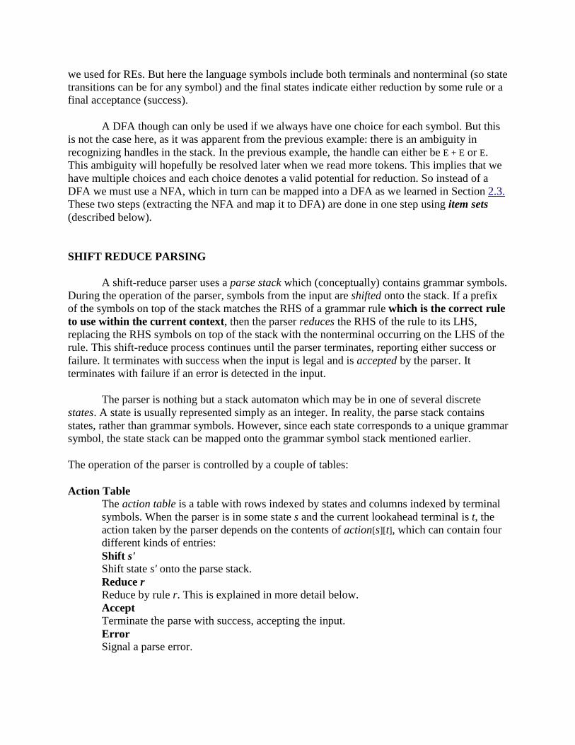
Action Table
The action table is a table with rows indexed by states and columns indexed by terminal
symbols. When the parser is in some state s and the current lookahead terminal is t, the
action taken by the parser depends on the contents of action[s][t], which can contain four
different kinds of entries:
Shift s' Shift state s' onto the parse stack.
Reduce r Reduce by rule r. This is explained in more detail below.
Accept Terminate the parse with success, accepting the input.
Error Signal a parse error.

Goto Table The goto table is a table with rows indexed by states and columns indexed by
nonterminal symbols. When the parser is in state s immediately after reducing by rule N,
then the next state to enter is given by goto[s][N].
The current state of a shift-reduce parser is the state on top of the state stack. The detailed
operation of such a parser is as follows:
1. Initialize the parse stack to contain a single state s0, where s0 is the distinguished initial
state of the parser.
2. Use the state s on top of the parse stack and the current lookahead t to consult the action
table entry action[s][t]:
If the action table entry is shift s' then push state s' onto the stack and advance the
input so that the lookahead is set to the next token.
If the action table entry is reduce r and rule r has m symbols in its RHS, then pop
m symbols off the parse stack. Let s' be the state now revealed on top of the parse
stack and N be the LHS nonterminal for rule r. Then consult the goto table and
push the state given by goto[s'][N] onto the stack. The lookahead token is not
changed by this step.
If the action table entry is accept, then terminate the parse with success.
If the action table entry is error, then signal an error.
3. Repeat step (2) until the parser terminates.
For example, consider the following simple grammar
0) $S: stmt <EOF> 1) stmt: ID ':=' expr 2) expr: expr '+' ID 3) expr: expr '-' ID 4) expr: ID which describes assignment statements like a:= b + c - d. (Rule 0 is a special augmenting production added to the grammar).
One possible set of shift-reduce parsing tables is shown below (sn denotes shift n, rn denotes
reduce n, acc denotes accept and blank entries denote error entries):
Parser Tables
0
1
2
Action Table Goto Table
ID ':=' '+' '-' <EOF> stmt expr
s1 g2
s3
s4
Relation Meaning
a <· b a yields precedence to b
a =· b a has the same precedence as b
3
4
5
6
7
8
9
10
s5 g6
acc acc acc acc acc
r4 r4 r4 r4 r4
r1 r1 s7 s8 r1
s9
s10
r2 r2 r2 r2 r2
r3 r3 r3 r3 r3
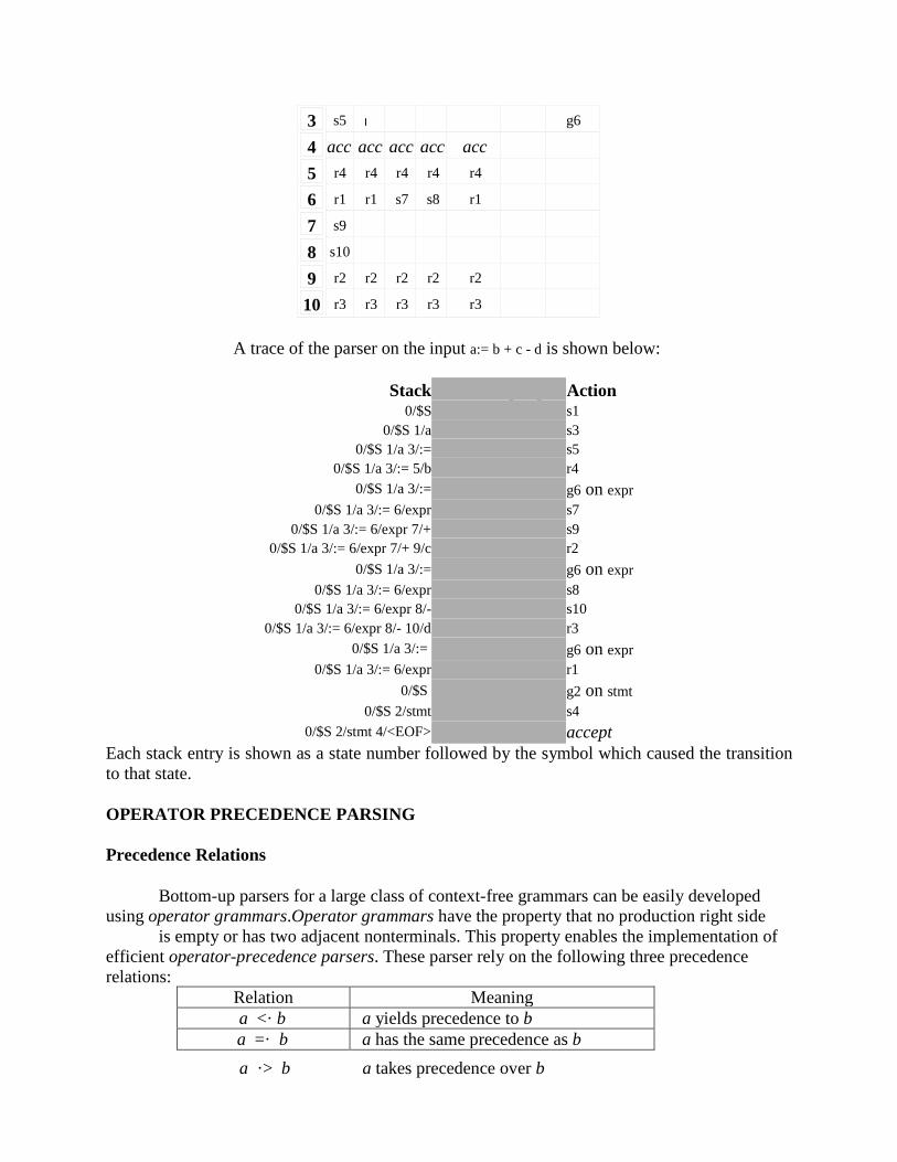
A trace of the parser on the input a:= b + c - d is shown below:
Stack Remaining Input Action
0/$S a:= b + c - d s1
0/$S 1/a := b + c - d s3
0/$S 1/a 3/:= b + c - d s5
0/$S 1/a 3/:= 5/b + c - d r4
0/$S 1/a 3/:= + c - d g6 on expr
0/$S 1/a 3/:= 6/expr + c - d s7
0/$S 1/a 3/:= 6/expr 7/+ c - d s9
0/$S 1/a 3/:= 6/expr 7/+ 9/c - d r2
0/$S 1/a 3/:= - d g6 on expr
0/$S 1/a 3/:= 6/expr - d s8
0/$S 1/a 3/:= 6/expr 8/- d s10
0/$S 1/a 3/:= 6/expr 8/- 10/d <EOF> r3
0/$S 1/a 3/:= <EOF> g6 on expr
0/$S 1/a 3/:= 6/expr <EOF> r1
0/$S <EOF> g2 on stmt
0/$S 2/stmt <EOF> s4
0/$S 2/stmt 4/<EOF> accept
Each stack entry is shown as a state number followed by the symbol which caused the transition
to that state. OPERATOR PRECEDENCE PARSING
Precedence Relations
Bottom-up parsers for a large class of context-free grammars can be easily developed
using operator grammars.Operator grammars have the property that no production right side is empty or has two adjacent nonterminals. This property enables the implementation of
efficient operator-precedence parsers. These parser rely on the following three precedence
relations:
a ·> b a takes precedence over b

These operator precedence relations allow to delimit the handles in the right sentential
forms: <· marks the left end, =· appears in the interior of the handle, and ·> marks the right
end.
id + * $
id ·> ·> ·>
+ <· ·> <· ·>
* <· ·> ·> ·>
$ <· <· <· ·>
Example: The input string:
id1 + id2 * id3
after inserting precedence relations becomes
$ <· id1 ·> + <· id2 ·> * <· id3 ·> $
Having precedence relations allows to identify handles as follows:
- scan the string from left until seeing ·>
- scan backwards the string from right to left until seeing <·
- everything between the two relations <· and ·> forms the handle Operator Precedence Parsing Algorithm
Initialize: Set ip to point to the first symbol of w$
Repeat: Let X be the top stack symbol, and a the symbol pointed to by ip
if $ is on the top of the stack and ip points to $ then return
else
by ip
Let a be the top terminal on the stack, and b the symbol pointed to
Let a be the top terminal on the stack, and b the symbol pointed to
if a <· b or a =· b then
push b onto the stack
advance ip to the next input symbol
else if a ·> b then
repeat
pop the stack
until the top stack terminal is related by <·
to the terminal most recently popped

end
else error()
else error()
Making Operator Precedence Relations
The operator precedence parsers usually do not store the precedence table with the
relations, rather they are implemented in a special way.Operator precedence parsers use
precedence functions that map terminal symbols to integers, and so the precedence relations
between the symbols are implemented by numerical comparison. Algorithm for Constructing Precedence Functions
1. Create functions fa for each grammar terminal a and for the end of string symbol;
2. Partition the symbols in groups so that fa and gb are in the same group if a =· b ( there
can be symbols in the same group even if they are not connected by this relation);
3. Create a directed graph whose nodes are in the groups, next for each symbols a and b
do: place an edge from the group of gb to the group of fa if a <· b, otherwise if a ·> b
place an edge from the group of fa to that of gb;
4. If the constructed graph has a cycle then no precedence functions exist. When there are
no cycles collect the length of the longest paths from the groups of fa and gb Example:
Consider the above table
id + * $
id ·> ·> ·>
+ <· ·> <· ·>
* <· ·> ·> ·>
$ <· <· <· ·>
Using the algorithm leads to the following graph:
gid
fid
f*
g*
g+
f+
f$
g$

from which we extract the following precedence functions:
id + * $
f 4 2 4 0
g 5 1 3 0
LR PARSERS LR parsing introduction
The "L" is for left-to-right scanning of the input and the "R" is for constructing a rightmost
derivation in reverse
LR-Parser
Advantages of LR parsing:
LR parsers can be constructed to recognize virtually all programming-language constructs for
which context-free grammars can be written. The LR parsing method is the most general non-backtracking shift-reduce parsing method
known, yet it can be implemented as efficiently as other shift-reduce methods. The class of grammars that can be parsed using LR methods is a proper subset of the class of
grammars that can be parsed with predictive parsers. An LR parser can detect a syntactic error as soon as it is possible to do so on a left-to-right scan
of the input. The disadvantage is that it takes too much work to constuct an LR parser by hand for a typical
programming-language grammar. But there are lots of LR parser generators available to make
this task easy.

The LR parsing algorithm
The schematic form of an LR parser is shown below.
The program uses a stack to store a string of the form s0X1s1X2...Xmsm where sm is on top. Each Xi
is a grammar symbol and each si is a symbol representing a state. Each state symbol summarizes
the information contained in the stack below it. The combination of the state symbol on top of
the stack and the current input symbol are used to index the parsing table and determine the shift-
reduce parsing decision. The parsing table consists of two parts: a parsing action function action
and a goto function goto. The program driving the LR parser behaves as follows: It determines sm
the state currently on top of the stack and ai the current input symbol. It then consults action[sm,
ai], which can have one of four values: shift s, where s is a state
reduce by a grammar production A -> b
accept
error
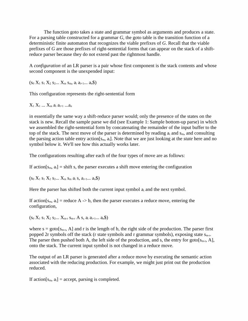
The function goto takes a state and grammar symbol as arguments and produces a state.
For a parsing table constructed for a grammar G, the goto table is the transition function of a
deterministic finite automaton that recognizes the viable prefixes of G. Recall that the viable
prefixes of G are those prefixes of right-sentential forms that can appear on the stack of a shift-
reduce parser because they do not extend past the rightmost handle. A configuration of an LR parser is a pair whose first component is the stack contents and whose
second component is the unexpended input: (s0 X1 s1 X2 s2... Xm sm, ai ai+1... an$)
This configuration represents the right-sentential form
X1 X1 ... Xm ai ai+1 ...an
in essentially the same way a shift-reduce parser would; only the presence of the states on the
stack is new. Recall the sample parse we did (see Example 1: Sample bottom-up parse) in which
we assembled the right-sentential form by concatenating the remainder of the input buffer to the
top of the stack. The next move of the parser is determined by reading ai and sm, and consulting
the parsing action table entry action[sm, ai]. Note that we are just looking at the state here and no
symbol below it. We'll see how this actually works later. The configurations resulting after each of the four types of move are as follows:
If action[sm, ai] = shift s, the parser executes a shift move entering the configuration
(s0 X1 s1 X2 s2... Xm sm ai s, ai+1... an$)
Here the parser has shifted both the current input symbol ai and the next symbol.
If action[sm, ai] = reduce A -> b, then the parser executes a reduce move, entering the
configuration, (s0 X1 s1 X2 s2... Xm-r sm-r A s, ai ai+1... an$)
where s = goto[sm-r, A] and r is the length of b, the right side of the production. The parser first
popped 2r symbols off the stack (r state symbols and r grammar symbols), exposing state sm-r.
The parser then pushed both A, the left side of the production, and s, the entry for goto[sm-r, A],
onto the stack. The current input symbol is not changed in a reduce move. The output of an LR parser is generated after a reduce move by executing the semantic action
associated with the reducing production. For example, we might just print out the production
reduced. If action[sm, ai] = accept, parsing is completed.

If action[sm, ai] = error, the parser has discovered an error and calls an error recovery routine. LR parsing algorithm
Input: Input string w and an LR parsing table with functions action and goto for a grammar G.
Output: If w is in L(G), a bottom-up parse for w. Otherwise, an error indication.
Method: Initially the parser has s0, the initial state, on its stack, and w$ in the input buffer.
repeat forever begin
let s be the state on top of the stack
and a the symbol pointed to by ip;
if action[s, a] = shift s' then begin
push a, then push s' on top of the stack; // <symbol, state> pair
advance ip to the next input symbol;
else if action[s, a] = reduce A -> b then begin
pop 2* |b| symbols off the stack;
let s' be the state now on top of the stack;
push A, then push goto[s', A] on top of the stack;
output the production A -> b; // for example
else if action[s, a] = accept then
return
else error();
end
Let's work an example to get a feel for what is going on,
An Example
(1) E -> E * B
(2) E -> E + B
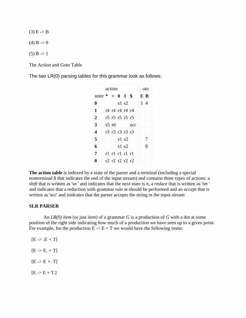
(3) E -> B
(4) B -> 0
(5) B -> 1
The Action and Goto Table The two LR(0) parsing tables for this grammar look as follows:
action g oto
state * + 0 1 $ E B
0 s1 s2 3 4
1 r4 r4 r4 r4 r4
2 r5 r5 r5 r5 r5
3 s5 s6 acc
4 r3 r3 r3 r3 r3
5 s1 s2 7
6 s1 s2 8
7 r1 r1 r1 r1 r1
8 r2 r2 r2 r2 r2
The action table is indexed by a state of the parser and a terminal (including a special
nonterminal $ that indicates the end of the input stream) and contains three types of actions: a
shift that is written as 'sn ' and indicates that the next state is n, a reduce that is written as 'rm '
and indicates that a reduction with grammar rule m should be performed and an accept that is
written as 'acc' and inidcates that the parser accepts the string in the input stream SLR PARSER
An LR(0) item (or just item) of a grammar G is a production of G with a dot at some
position of the right side indicating how much of a production we have seen up to a given point.
For example, for the production E -> E + T we would have the following items:
[E -> .E + T]
[E -> E. + T]
[E -> E +. T]
[E -> E + T.]

We call them LR(0) items because they contain no explicit reference to lookahead. More on this
later when we look at canonical LR parsing. The central idea of the SLR method is first to
construct from the grammar a deterministic finite automaton to recognize viable prefixes. With
this in mind, we can easily see the following: the symbols to the left of the dot in an item are on
up until the time when we have the dot to the right of the last symbol of the production, we have
a viable prefix .when the dot reaches the right side of the last symbol of the production, we have
a handle for the production and can do a reduction (the text calls this a completed item; similarly
it calls [E -> .E + T] an initial item). an item is a summary of the recent history of a parse (how so?)
items correspond to the states of a NFA (why an NFA and not a DFA?).
Now, if items correspond to states, then there must be transitions between items
(paralleling transitions between the states of a NFA). Some of these are fairly obvious. For
example, consider the transition from [E -> .(E)] to [E -> (.E)] which occurs when a "(" is shifted
onto the stack. In a NFA this would correspond to following the arc labelled "(" from the state
corresponding to [E -> .(E)] to the state corresponding to [E -> (.E)]. Similarly, we have [T -> .F]
and [T -> F.] which occurs when F is produced as the result of a reduction and pushed onto the
stack. Other transitions can occur on e-transitions.
The insight that items correspond to states leads us to the explanation for why we need e-
transitions.
Consider a transition on symbol X from [A -> a.Xg] to [A -> aX.g]. In a transition diagram
this looks like:
If X is a terminal symbol, this transition corresponds to shifting X from the input buffer to
the top of the stack. Things are more complicated if X is a nonterminal because nonterminals cannot appear in the
input and be shifted onto the stack as we do with terminals. Rather, nonterminals only appear on
the stack as the result of a reduction by some production X -> b.
To complete our understanding of the creation of a NFA from the items, we need to decide on
the choices for start state and final states.

We'll consider final states first. Recall that the purpose of the NFA is not to recognize strings,
but to keep track of the current state of the parse, thus it is the parser that must decide when to do
an accept and the NFA need not contain that information. For the start state, consider the initial configuration of the parser: the stack is empty and we want
to recognize S, the start symbol of the grammar. But there may be many initial items [S -> .a]
from which to choose. To solve the problem, we augment our grammar with a new production S' -> S, where S' is the
new start symbol and [S' -> .S] becomes the start state for the NFA. What will happen is that
when doing the reduction for this production, the parser will know to do an accept. The following example makes the need for e-transitions and an augmented grammar more
concrete. Consider the following augmented grammar:
E' -> E
E -> E + T
E -> T
T -> T * F
T -> F
F -> (E)
F -> id
A quick examination of the grammar reveals that any legal string must begin with either ( or id,
resulting in one or the other being pushed onto the stack. So we would have either the state transition [F -> .(E)] to [F -> (.E)] or the transition from [F
-> .id] to [F -> id.]. But clearly to make either of these transitions we must already be in the corresponding state ([F
-> .(E)] or [F -> .id]). Recall, though, that we always begin with our start state [E' -> E] and note that there is no
transition from the start state to either [F -> .(E)] or [F -> .id]. To get from the start state to one of these two states without consuming anything from the input
we must have e-transitions. The example from the book makes this a little clearer. We want to parse "(id)".

items and e-transitions
Stack State Comments
Empty [E'-> .E] can't go anywhere from here
e-
transition
so we follow an e-transition
Empty [F -> .(E)] now we can shift the (
(
[F -> (.E)]
building the handle (E); This state says: "I have ( on the stack and expect the
input to give me tokens that can eventually be reduced to give me the rest of the
handle, E)."
constructing the LR parsing table
To construct the parser table we must convert our NFA into a DFA.
*** The states in the LR table will be the e-closures of the states corresponding to the items!!
SO...the process of creating the LR state table parallels the process of constructing an equivalent
DFA from a machine with e-transitions. Been there, done that - this is essentially the subset
construction algorithm so we are in familiar territory here! We need two operations: closure()
and goto().
closure()
If I is a set of items for a grammar G, then closure(I) is the set of items constructed from I by the
two rules:
Initially every item in I is added to closure(I)
If A -> a.Bb is in closure(I), and B -> g is a production, then add the initial item [B -> .g] to I, if it
is not already there. Apply this rule until no more new items can be added to closure(I).
From our grammar above, if I is the set of one item {[E'-> .E]}, then closure(I) contains:
I0: E' -> .E
E -> .E + T
E -> .T
T -> .T * F
T -> .F
F -> .(E)

F -> .id
goto()
goto(I, X), where I is a set of items and X is a grammar symbol, is defined to be the closure of
the set of all items [A -> aX.b] such that [A -> a.Xb] is in I. The idea here is fairly intuitive: if I is the set of items that are valid for some viable prefix g, then
goto(I, X) is the set of items that are valid for the viable prefix gX. Building a DFA from the LR(0) items
Now we have the tools we need to construct the canonical collection of sets of LR(0) items for
an augmented grammar G'. Sets-of-Items-Construction: to construct the canonical collection of sets of LR(0) items for
augmented grammar G'.
procedure items(G')
begin
C := {closure({[S' -> .S]})};
repeat
for each set of items in C and each grammar symbol X
such that goto(I, X) is not empty and not in C do
add goto(I, X) to C;
until no more sets of items can be added to C end;
algorithm for constructing an SLR parsing table
Input: augmented grammar G'
Output: SLR parsing table functions action and goto for G'
Method: Construct C = {I0, I1 , ..., In} the collection of sets of LR(0) items for G'.
State i is constructed from Ii:

if [A -> a.ab] is in Ii and goto(Ii, a) = Ij, then set action[i, a] to "shift j". Here a must be a terminal. if [A -> a.] is in Ii, then set action[i, a] to "reduce A -> a" for all a in FOLLOW(A). Here A may
not be S'. if [S' -> S.] is in Ii, then set action[i, $] to "accept"
If any conflicting actions are generated by these rules, the grammar is not SLR(1) and the
algorithm fails to produce a parser. The goto transitions for state i are constructed for all nonterminals A using the rule: If goto(Ii, A)
= Ij, then goto[i, A] = j. All entries not defined by rules 2 and 3 are made "error".
The inital state of the parser is the one constructed from the set of items containing [S' -> .S].
Example: Build the canonical LR(0) collections and DFAs for the following grammars:
Ex 1:
S -> ( S ) S | e
Ex 2:
S -> ( S ) | a
Ex 3:
E' -> E
E -> E + T
E -> T
T -> T * F
T -> F
F -> ( E )
F -> id Here is what the corresponding DFA looks like:

Dealing with conflicts
Recall that the actions of a parser are one of: 1) shift, 2) reduce, 3) accept, and 4) error. A grammar is said to be a LR(0) grammar if rules 1 and 2 are unambiguous. That is, if a state
contains a completed item [A -> a.], then it can contain no other items. If, on the other hand, it
also contains a "shift" item, then it isn't clear if we should do the reduce or the shift and we have
a shift-reduce conflict. Similarly, if a state also contains another completed item, say, [B -> b.],
then it isn't clear which reduction to do and we have a reduce-reduce conflict. Constructing the action and goto table as is done for LR(0) parsers would give the following item
sets and tables: Item set 0
S → · E
+ E → · 1 E
+ E → · 1
Item set 1

E → 1 · E
E → 1 ·
+ E → · 1 E + E → · 1
Item set 2
S → E ·
Item set 3
E → 1 E ·
The action and goto tables:
action goto
state 1 $ E
0 s1 2
1 s2/r2 r2 3
2 acc
3 r1 r1
As can be observed there is a shift-reduce conflict for state 1 and terminal '1'. For shift-reduce conflicts there is a simple solution used in practice: always prefer the shift
operation over the reduce operation. This automatically handles, for example, the dangling else
ambiguity in if-statements. See the book's discussion on this. Reduce-reduce problems are not so easily handled. The problem can be characterized generally
as follows: in the SLR method, state i calls for reducing by A -> a if the set of items Ii contains
item [A -> a.] (a completed item) and a is in FOLLOW(A). But sometimes there is an alternative
([B -> a.]) that could also be taken and the reduction is made. CANONICAL LR PARSER
Canonical LR parsing
By splitting states when necessary, we can arrange to have each state of an LR parser
indicate exactly which input symbols can follow a handle a for which there is a possible
reduction to A. As the text points out, sometimes the FOLLOW sets give too much information
and doesn't (can't) discriminate between different reductions.

The general form of an LR(k) item becomes [A -> a.b, s] where A -> ab is a production
and s is a string of terminals. The first part (A -> a.b) is called the core and the second part is the
lookahead. In LR(1) |s| is 1, so s is a single terminal.
A -> ab is the usual righthand side with a marker; any a in s is an incoming token in
which we are interested. Completed items used to be reduced for every incoming token in
FOLLOW(A), but now we will reduce only if the next input token is in the lookahead set s.
SO...if we get two productions A -> a and B -> a, we can tell them apart when a is a handle on
the stack if the corresponding completed items have different lookahead parts.
Furthermore, note that the lookahead has no effect for an item of the form [A -> a.b, a] if
b is not e. Recall that our problem occurs for completed items, so what we have done now is to
say that an item of the form [A -> a., a] calls for a reduction by A -> a only if the next input
symbol is a. More formally, an LR(1) item [A -> a.b, a] is valid for a viable prefix g if there is a
derivation S =>*
s abw, where g = sa, and
either a is the first symbol of w, or w is e and a is $.
algorithm for construction of the sets of LR(1) items
Input: grammar G'
Output: sets of LR(1) items that are the set of items valid for one or more viable prefixes of G'
Method:
closure(I)
begin
repeat
for each item [A -> a.Bb, a] in I,
each production B -> g in G',
and each terminal b in FIRST(ba)
such that [B -> .g, b] is not in I do
add [B -> .g, b] to I;
until no more items can be added to I; end;

goto(I, X) begin
let J be the set of items [A -> aX.b, a] such that
[A -> a.Xb, a] is in I
return closure(J);
end;
procedure items(G')
begin
C := {closure({S' -> .S, $})};
repeat
for each set of items I in C and each grammar symbol X such
that goto(I, X) is not empty and not in C do
add goto(I, X) to C
until no more sets of items can be added to C; end;
An example,
Consider the following grammer,
S’->S
S->CC
C->cC
C->d
Sets of LR(1) items I0: S’->.S,$

S->.CC,$
C->.Cc,c/d
C->.d,c/d I1:S’->S.,$
I2:S->C.C,$
C->.Cc,$
C->.d,$
I3:C->c.C,c/d
C->.Cc,c/d
C->.d,c/d
I4: C->d.,c/d
I5: S->CC.,$
I6: C->c.C,$
C->.cC,$
C->.d,$ I7:C-
>d.,$ I8:C-
>cC.,c/d
I9:C->cC.,$
Here is what the corresponding DFA looks like

Parsing
Table:state
c
d
$
S
C
0
S3
S4
1
2
1
acc
2 S6 S7 5
3
S3
S4
8
4
R3
R3
5
R1
6
S6
S7
9
7
R3
8
R2
R2
9
R2
algorithm for construction of the canonical LR parsing table
Input: grammar G'
Output: canonical LR parsing table functions action and goto

Construct C = {I0, I1 , ..., In} the collection of sets of LR(1) items for G'.
State i is constructed from Ii:
if [A -> a.ab, b>] is in Ii and goto(Ii, a) = Ij, then set action[i, a] to "shift j". Here a must be a
terminal. if [A -> a., a] is in Ii, then set action[i, a] to "reduce A -> a" for all a in FOLLOW(A). Here A may
not be S'. if [S' -> S.] is in Ii, then set action[i, $] to "accept"
If any conflicting actions are generated by these rules, the grammar is not LR(1) and the
algorithm fails to produce a parser. The goto transitions for state i are constructed for all nonterminals A using the rule: If goto(Ii, A)
= Ij, then goto[i, A] = j. All entries not defined by rules 2 and 3 are made "error".
The inital state of the parser is the one constructed from the set of items containing [S' -> .S, $].
Example: Let's rework the following grammar:
A -> ( A ) | a Every SLR(1) grammar is an LR(1) grammar. The problem with canonical LR parsing is that it
generates a lot of states. This happens because the closure operation has to take the lookahead
sets into account as well as the core items. The next parser combines the simplicity of SLR with the power of LR(1).
LALR PARSER
We begin with two observations. First, some of the states generated for LR(1) parsing
have the same set of core (or first) components and differ only in their second component, the
lookahead symbol. Our intuition is that we should be able to merge these states and reduce the
number of states we have, getting close to the number of states that would be generated for
LR(0) parsing.
This observation suggests a hybrid approach: We can construct the canonical LR(1) sets
of items and then look for sets of items having the same core. We merge these sets with common
cores into one set of items. The merging of states with common cores can never produce a
shift/reduce conflict that was not present in one of the original states because shift actions
depend only on the core, not the lookahead. But it is possible for the merger to produce a
reduce/reduce conflict.

state c d $
0 S36 S47
Our second observation is that we are really only interested in the lookahead symbol in
places where there is a problem. So our next thought is to take the LR(0) set of items and add
lookaheads only where they are needed. This leads to a more efficient, but much more
complicated method. Algorithm for easy construction of an LALR table
Input: G'
Output: LALR parsing table functions with action and goto for G'.
Method:
Construct C = {I0, I1 , ..., In} the collection of sets of LR(1) items for G'. For each core present among the set of LR(1) items, find all sets having that core and replace
these sets by the union. Let C' = {J0, J1 , ..., Jm} be the resulting sets of LR(1) items. The parsing actions for state i are
constructed from Ji in the same manner as in the construction of the canonical LR parsing table.
If there is a conflict, the grammar is not LALR(1) and the algorithm fails. The goto table is constructed as follows: If J is the union of one or more sets of LR(1) items, that
is, J = I0U I1 U ... U Ik, then the cores of goto(I0, X), goto(I1, X), ..., goto(Ik, X) are the same, since
I0, I1 , ..., Ik all have the same core. Let K be the union of all sets of items having the same core as
goto(I1, X). Then goto(J, X) = K. Consider the above example,
I3 & I6 can be replaced by their union
I36:C->c.C,c/d/$
C->.Cc,C/D/$
C->.d,c/d/$
I47:C->d.,c/d/$
I89:C->Cc.,c/d/$
Parsing Table
S C
1 2

1 Acc
2 S36 S47
36 S36 S47
47 R3 R3
5 R1
89 R2 R2 R2
5
89
handling errors The LALR parser may continue to do reductions after the LR parser would have spotted an error,
but the LALR parser will never do a shift after the point the LR parser would have discovered
the error and will eventually find the error.
UNIT III - INTERMEDIATE CODE GENERATION
INTERMEDIATE LANGUAGES

In Intermediate code generation we use syntax directed methods to translate the source
program into an intermediate form programming language constructs such as declarations,
assignments and flow-of-control statements.
There are three types of intermediate representation:-
1. Syntax Trees
2. Postfix notation
3. Three Address Code
Semantic rules for generating three-address code from common programming language
constructs are similar to those for constructing syntax trees of for generating postfix notation.
Graphical Representations
A syntax tree depicts the natural hierarchical structure of a source program. A DAG (Directed
Acyclic Graph) gives the same information but in a more compact way because common sub-
expressions are identified. A syntax tree for
the assignment statement a:=b*-c+b*-c appear in the figure.
Postfix notation is a linearized representation of a syntax tree; it is a list of the nodes of the in
which a node appears immediately after its children. The postfix notation for the syntax tree in
the fig is
a b c uminus + b c uminus * + assign
The edges in a syntax tree do not appear explicitly in postfix notation. They can be recovered in
the order in which the nodes appear and the no. of operands that the operator at a node expects.
The recovery of edges is similar to the evaluation, using a staff, of an expression in postfix
notation.
fig.
Syntax tree for assignment statements are produced by the syntax directed definition in
Syntax tree for assignment statements are produced by the syntax directed definition in
Production Semantic Rule
S id := E S.nptr := mknode( ‘assign’, mkleaf(id, id.place), E.nptr)
E E1 + E2 E.nptr := mknode(‘+’, E1.nptr ,E2.nptr)
E E1 * E2 E.nptr := mknode(‘* ’, E1.nptr ,E2.nptr)
E - E1 E.nptr := mkunode(‘uminus’, E1.nptr)
E ( E1 ) E.nptr := E1.nptr
E id E.nptr := mkleaf(id, id.place)

0
id
b
1
id
c
2
uminus
1
3
*
0
2
4
id
b
5
id
c
6
uminus
5
7
*
4
6
8
+
3
7
9
id
a
1
assign
9
8
1
……
Three-Address Code
Three-address code is a sequence of statements of the general form
X:= Op Z
where x, y, and z are names, constants, or compiler-generated temporaries; op stands for any
operator, such as a fixed- or floating-point arithmetic operator, or a logical operator on Boolean-
valued data. Note that no built-up arithmetic expressions are permitted, as there is only one
operator on the right side of a statement. Thus a source language expression like x+y*z might be
translated into a sequence
Z
X +
where t1 and t2 are compiler-generated temporary names. This unraveling cf complicated
arithmetic expressions and of nested flow-of-control statements makes three-address code
desirable for target code generation and optimization. The use of names for the intermediate
values computed by a program allow- three-address code to be easily rearranged – unlike postfix
notation. three-address code is a linearized representation of a syntax tree or a dag in which
explicit names correspond to the interior nodes of the graph. The syntax tree and dag in Fig. 8.2
are represented by the three-address code sequences in Fig. 8.5. Variable names can appear
directly in three-address statements, so Fig. 8.5(a) has no statements corresponding to the leaves

in Fig. 8.4. Code for syntax tree
t1 := -c
t2 := b * t1
t3 := -c
t4 := b * t3
t5 := t2 + t4
a := t5 Code for DAG
t1 := -c
t2 := b * t1
t5 := t2 + t2
a := t5
The reason for the term ”three-address code” is that each statement usually contains three
addresses, two for the operands and one for the result. In the implementations of three-address
code given later in this section, a programmer-defined name is replaced by a pointer tc a symbol-
table entry for that name.
Types Of Three-Address Statements
Three-address statements are akin to assembly code. Statements can have symbolic labels
and there are statements for flow of control. A symbolic label represents the index of a three-
address statement in the array holding inter- mediate code. Actual indices can be substituted for
the labels either by making a separate pass, or by using ”back patching,” discussed in Section
8.6. Here are the common three-address statements used in the remainder of this book:
1. Assignment statements of the form x: = y op z, where op is a binary arithmetic or logical
operation.
2. Assignment instructions of the form x:= op y, where op is a unary operation. Essential unary
operations include unary minus, logical negation, shift operators, and conversion operators that,
for example, convert a fixed-point number to a floating-point number.
3. Copy statements of the form x: = y where the value of y is assigned to x.
4. The unconditional jump goto L. The three-address statement with label L is the next to be
executed.
5. Conditional jumps such as if x relop y goto L. This instruction applies a relational operator (<,
=, >=, etc.) to x and y, and executes the statement with label L next if x stands in relation relop to
y. If not, the three-address statement following if x relop y goto L is executed next, as in the
usual sequence.
6. param x and call p, n for procedure calls and return y, where y representing a returned value is
optional. Their typical use is as the sequence of three-address statements
param x1
param x2
param xn
call p, n

generated as part of a call of the procedure p(x,, x~,..., x”). The integer n indicating the number
of actual parameters in ”call p, n” is not redundant because calls can be nested. The
implementation of procedure calls is outline d in Section 8.7.
7. Indexed assignments of the form x: = y[ i ] and x [ i ]: = y. The first of these sets x to the value
in the location i memory units beyond location y. The statement x[i]:=y sets the contents of the
location i units beyond x to the value of y. In both these instructions, x, y, and i refer to data
objects.
8. Address and pointer assignments of the form x:= &y, x:= *y and *x: = y. The first of these
sets the value of x to be the location of y. Presumably y is a name, perhaps a temporary, that
denotes an expression with an I-value such as A[i, j], and x is a pointer name or temporary. That
is, the r-value of x is the l-value (location) of some object!. In the statement x: = ~y, presumably
y is a pointer or a temporary whose r- value is a location. The r-value of x is made equal to the
contents of that location. Finally, +x: = y sets the r-value of the object pointed to by x to the r-
value of y.
The choice of allowable operators is an important issue in the design of an intermediate
form. The operator set must clearly be rich enough to implement the operations in the source
language. A small operator set is easier to implement on a new target machine. However, a
restricted instruction set may force the front end to generate long sequences of statements for
some source, language operations. The optimizer and code generator may then have to work
harder if good code is to be generated. Implementations of three-Address Statements
A three-address statement is an abstract form of intermediate code. In a compiler, these
statements can be implemented as records with fields for the operator and the operands. Three
such representations are quadruples, triples, and indirect triples.
Quadruples
A quadruple is a record structure with four fields, which we call op, arg l, arg 2, and
result. The op field contains an internal code for the operator. The three-address statement x:= y
op z is represented by placing y in arg 1. z in arg 2. and x in result. Statements with unary
operators like x: = – y or x: = y do not use arg 2. Operators like param use neither arg2 nor
result. Conditional and unconditional jumps put the target label in result. The quadruples in Fig.
H.S(a) are for the assignment a: = b+ – c + b i – c. They are obtained from the three-address code
in Fig. 8.5(a). The contents of fields arg 1, arg 2, and result are normally pointers to the symbol-
table entries for the names represented by these fields. If so, temporary names must be entered
into the symbol table as they are created.
Triples
To avoid entering temporary names into the symbol table. we might refer to a temporary

op Arg1 Arg2 Result
(0
)
uminus c t1
(1
)
* b t1 t2
(2
)
uminus c t3
(3
)
* b t3 t4
(4
)
+ t2 t4 t5
(5
)
:= t5 a
op Arg1 Arg2
(0
)
uminus c
(1
)
* b (0)
(2
)
uminus c
(3
)
* b (2)
(4
)
+ (1) (3)
(5
)
:= a (4)
value bi the position of the statement that computes it. If we do so, three-address statements can
be represented by records with only three fields: op, arg 1 and arg2, as in Fig. 8.8(b). The fields
arg l and arg2, for the arguments of op, are either pointers to the symbol table (for programmer-
defined names or constants) or pointers into the triple structure (for temporary values). Since
three fields are used, this intermediate code format is known as triples.’ Except for the treatment
of programmer-defined names, triples correspond to the representation of a syntax tree or dag by
an array of nodes, as in Fig. 8.4.
Parenthesized
numbers represent
pointers into the triple
structure, while symbol-
table pointers are
represented by the names
themselves. In practice,
the information needed
to interpret the different
kinds of entries in the arg 1 and arg2 fields can be encoded into
the op field or some additional fields. The triples in Fig. 8.8(b) correspond to the quadruples in
Fig. 8.8(a). Note that the copy statement a:= t5 is encoded in the triple representation by placing
a in the arg 1 field and using the operator assign. A ternary operation like x[ i ]: = y requires two
entries in the triple structure, as shown in Fig. 8.9(a), while x: = y[i] is naturally represented
Indirect Triples
Another implementation of three-address code that has been considered is that of listing
pointers to triples, rather than listing the triples themselves. This implementation is naturally
called indirect triples. For example, let us use an array statement to list pointers to triples in the
desired order. Then the triples in Fig. 8.8(b) might be represented as in Fig. 8.10.
DECLARATIONS
As the sequence of declarations in a procedure or block is examined, we can lay out
storage for names local to the procedure. For each local name, we create a symbol-table entry
with information like the type and the relative address of the storage for the name. The relative
address consists of an offset from the base of the static data area or the field for local data in an
activation record. When the front end generates addresses, it may have a target machine in mind.
Suppose that addresses of consecutive integers differ by 4 on a byte- addressable machine. The
address calculations generated by the front end may therefore include multiplications by 4. The
instruction set of the target machine may also favor certain layouts of data objects, and hence

their addresses. We ignore alignment of data objects here, Example 7.3 shows how data objects
are aligned by two compilers. Declarations in a Procedure
The syntax of languages such as C, Pascal, and Fortran, allows all the declarations in a
single procedure to be processed as a group. In this case, a global variable, say offset, can keep
track of the next avai1able relative address. In the translation scheme of Fig. S.I1 non-terminal P
generates a sequence of declarations of the form id: T. Before ’.he first declaration is considered,
offset is set to 0. As each new name is seen, that name is entered in the symbol table with offset
equal to the current value of offset, and offset is incremented by the width of the data object
denoted by that name. The procedure enter(name, type, offset) creates a symbol-table entry for
name, gives it type and relative address offset in its data area. We use synthesized attributes type
and width for non-terminal T to indicate the type and width, or number of memory units taken by
objects of that type. Attribute type represents a type expression constructed from the basic types
integer and real by applying the type constructors pointer and array, as in Section 6.l. If type
expressions are represented by graphs, then attribute type might be a pointer to the node
representing a type expression. In Fig. 8. I , integers have width 4 and real have width 8. The
width of an array is obtained by multiplying the width of each element by the number of
elements in the array.- The width of each pointer is assumed to be 4. P D
D D ; D
D id : T {enter (id.name, T.type, offset);
Offset:= offset + T.width }
T integer {T.type :=integer;
T.width :=4}
T real {T.type := real;
T.width := 8}
T array [num ] of T1 {T.type :=array(num.val, T1.type);
T.width :=num.val X T1.width}
T ̂ T1 {T.type :=pointer (T.type);
T.width:=4}
In Pascal and C, a pointer may be seen before we learn the type of the object
pointed to Storage allocation for such types is simpler if all pointers have the same width. The
initialization of offset in the translation scheme of Fig. 8.1 is more evident if the first production
appears on one line as:
P {offset:= 0 } D
Non-terminals generating a. called marker non-terminals in Section 5.6, can be used to rewrite
productions so that all actions appear at the ends of right sides. Using a marker non-terminal M,
(8.2) can be restated as:
P M D
M ε (offset:= 0}

Keeping Track of Scope Information
In a language with nested procedures, names local to each procedure can be
assigned relative addresses using the approach of Fig. 8.11 . When a nested procedure is seen,
processing of declarations in the enclosing procedure is temporarily suspended. This approach
will he illustrated by adding semantic rules to the following language.
P D
D D;D | id: T proc id; D;S
The production for non-terminals S for statements and T for types are not shown because we
focus on declarations. The non-terminal T has synthesized attributes type and width, as in the
translation scheme The semantic rules are defined in terms of the following operations:
I. mktable(previous) creates a new symbol table and returns a pointer to the new table. The
argument previous points to a previously created symbol table, presumably that for the enclosing
procedure. The pointer previous is placed in a header for the new symbol table, along with
additional information such as the nesting depth of a procedure. We can also number the
procedures in the order they are declared and keep this number in the header.
2. enter(table, name, type, offset) creates a new entry for name name in the symbol table pointed
to by table. Again, enter places type and relative address offset in fields within the entry.
3. addwidth(table, width) records the cumulative width of all the entries table in the header
associated with this symbol table.
4. enterproc (table, name, newtable) creates a new entry for procedure name in the symbol table
pointed to by table. The argument newtable points to the symbol table for this procedure name.
The translation scheme in Fig. S. l3 shows how data can be laid out in one pass, using a stack
tblptr to hold pointers to symbol tables of the enclosing procedures. With the symbol tables ot’
Fig. 8.12, tblptr will contain pointers to the tables for -ort, quicksort, and partition when the
declarations in partition are considered. The pointer to the current symbol table is on top. The
other stack offset is the natural generalization to nested procedures of attribute offset in Fig. 8. l
I. The top element of offset is the next available relative address for a local of the current
procedure. All semantic actions in the sub-trees for B and C in
A B C { actionA}
are done before actionA the end of the production occurs. Hence, the action associated with the
marker M in Fig. 8.l3 is the first to be done. The action for non-terminal M initializes stack
tblptr with a symbol table for the outermost scope, created by operation mktable(nil). The action
also pushes relative address 0 onto stack offset. The non-terminal V plays a similar role when a
procedure declaration appears. Its action uses the operation mktable(top(tblptr)) to create a new
symbol table. Here the argument top(tblptr) gives the enclosing scope of the new table. A pointer
to the new table is pushed above that for the enclosing scope. Again, 0 is pushed onto offset.
For each variable declaration id: T. an entry is created for id in the current symbol table.
This declaration leaves the stack pointer unchanged; the top of stack offset is incremented by
T.width. when the action on the right side of D proc id: N D,; S occurs. the width of all
declarations generated by D1 is on top of stack offset.’, it is recorded using addwidth. and
offset are then popped, and we revert to examining the declarations in the closing procedure. At

this point, the name of the enclosed procedure is entered into the symbol table of its enclosing
procedure.
P M D {addwidth(top(tblptr), top(offset));
Pop(tblptr); pop(offset)}
M ε { t := mktable(nil);
Push(t,tblptr); push(0,offset)}
D D1 ;D2
D proc id ; N D1 ;S { t := top(tblptr);
addwidth(t.top(offset));
pop(tblptr); pop(offset);
enterproc(top(tblptr), id.name, t)}
D id : T {enter(top(tblptr),id.name,T.type,top(offset));
top(offset) := top(offset) +T.width }
N ε { t := mktable(top(tblptr));
Push(t, tblptr); push(0, offset)}
Field Names in Records
The following production allows non-terminal T to generate records in addition to basic
types, pointers, and arrays:
T record D end
The actions in the translation scheme of Fig. S.I4 emphasize the similarity between the layout of
records as a language construct and activation records. Since procedure definitions do not affect
the width computations in Fig. 8.13, we overlook the fact that the above production also allows
procedure definitions to appear within records.
T record L D end {T.type := record(top(tblptr));
T.width := top(offset);
Pop(tblptr); pop(offset) }
L ε { t:= mktable(nil);
Push(t, tblptr); push (0, offset) }
After the keyword record is seen, the acting associated with the marker
creates a new symbol table for the field names. A pointer to this symbol table is pushed onto
stack tblptr and relative address 0 is pushed onto stack . The action for D id: T in Fig. 8.13
therefore enters information about the field name id into the symbol table for the record.
Furthermore, the top of stack will hold the width of all the data objects within the record after
the fields have been examined. The action following end in Fig. 8. 14 returns the width as
synthesized attribute T.width. The type T.type is obtained by applying the constructor record to
the pointer to the symbol table for this record.

ASSIGNMENT STATEMENTS
Type Conversions Within Assignments
E.place := newtemp;
if E1.type = integer and E2.type = integer then begin
emit(E.place’:=’ E1.place ’int+’ E2.place);
E.type: = integer
end
else if E1.type = real and E2.type = real then begin
emit (E.place ’:=’ E1.place ’real +’ E2.place);
E.type := real
end
else if E1.type = integer and E2.type = real then begin
u := newtemp;
emit(u ’:=’ ’inttoreal’ E1.place);
emit(E.place ’:=’ u ’real+’ E2.place);
E.type:= real
end
else if E1.type = real and E2.type = integer then begin
u := newtemp;
emit(u ’:=’ ’inttoreal’ E2.place);
emit(E.place ’:=’ E1.place ’real+’ u);
E.type: = real
end
else
E.type:= type error;
Fig. 8.19. Semantic action for E E1 + E2.
The semantic action of Fig. 8. l9 uses two attributes E.place and E.type for the non-terminal E.
As the number of types subject to conversion increases. The number of cases that arise increases
quadratically (or worse, if there are operators with more than two arguments). Therefore with
large numbers of types, careful organization of the semantic actions becomes more important. Accessing Fields in Records
The compiler must keep track of both the types and relative addresses of the fields of a
record. An advantage of keeping this information in symbol-table entries for the field names is
that the routine for looking up names in the symbol table can also be used for field names. With
this in mind, a separate symbol table was created for each record type by the semantic actions in
Fig. 8.14. lf r is a pointer to the symbol table for a record type, then the type record(t) formed by
applying the constructor record to the pointer was returned as T.type We use the expression
p↑.info + 1
to illustrate how a pointer to the symbol table can be extracted from an attribute E.type. From the
operations in this expression it follows that p must be a pointer to a record with a field name info
whose type is arithmetic. If types are constructed as in Fig. 8.13 and 8.14, the type of p must be

given by a type expression
pointer (record(t))
The type of pt is then record(t), from which t can be extracted. The field name info is looked up
in the symbol table pointed to by t. BOOLEAN EXPRESSIONS
Boolean expressions
Two choices for implementation:
• Numerical representation: encode true and false values numerically,
and then evaluate analogously to an arithmetic expression.
. 1: true; 0: false.
. 6= 0: true; 0: false.
• Flow of control: representing the value of a boolean expression by a
position reached in a program.
Short-circuit code.
• Generate the code to evaluate a boolean expression in such a way that
it is not necessary for the code to evaluate the entire expression.
• if a1 or a2
. a1 is true, then a2 is not evaluated.
• Similarly for “and”.
• Side effects in the short-circuited code are not carried out.
. Example: (a > 1) and (p function(· · · ) > 100)
. if the calling of p function() creates some side effects, then this side
effect is not carried out in the case of (a > 1) being false.
Numerical representation
B ! id1 relop id2
• {B.place := newtemp();
• gen(“if”, id1.place,relop.op, id2.place,“goto”,nextstat+3);
• gen(B.place,“:=”,“0”);
• gen(“goto”,nextstat+2);
• gen(B.place,“:=”,“1”);}
Example: translating (a < b or c < d and e < f) using no
short-circuit evaluation.
100: if a < b goto 103
101: t1 := 0
102: goto 104
103: t1 := 1 /* true */
104: if c < d goto 107
105: t2 := 0 /* false */
106: goto 108
107: t2 := 1
108: if e < f goto 111
109: t3 := 0
110: goto 112
111: t3 := 1

112: t4 := t2 and t3
113: t3 := t1 or t4
Flow of control representation
Production Semantic actions
B ! id1 relop id2 B.true := newlabel();
B.false := newlabel();
B.code := gen(“if”,id1,relop,id2,“goto”,
B.true,“else”,“goto”,B.false) || gen(B.true,“:”)
S ! if B then S1 S.code := B.code || S1.code
|| gen(B.false,“:”)
|| is the code concatenation operator.
Uses only S-attributed definitions. CASE STATEMENTS
case E of V 1 : S 1 ... Vn: Sn end
One translation approach:
t :=expr
jump test
L 1 : code for S1; jump next
L 2 : code for S 2; jump next
...
Ln: code for Sn jump next
test: if t = V1 jump L 1
if t = V2 jump L 2
...
if t = Vn jump Ln
code to raise run-time exception
next:
Another translation approach: t :=expr
check t in bounds of 0…n-1 if not code to raise run-time exception
jump jtable + t
L 1 : code for S1; jump next
L 2 : code for S 2; jump next
...
Ln: code for Sn jump next
Jtable: jump L 1
jump L 2
...
jump Ln
next:

BACK PATCHING
The main problem in generating three address codes in a single pass for Boolean
expressions and flow of control statements is that we may not know the labels that
control must go to at the time jump statements are generated.
This problem is solved by generating a series of branch statements with the targets of the
jumps temporarily left unspecified.
Each such statement will be put on a list of goto statements whose labels will be filled in
when the proper label can be determined.
This subsequent filling of addresses for the determined labels is called BACKPATCHING
For implementing Backpatching ,we generate quadruples into a quadruple array and
Labels are indices to this array.
To manipulate list if labels ,we use three functions: makelist(i),merge(p1,p2) and
backpatch(p,i).
makelist(i) : creates a new list containing only i, an index into the array of quadruples and
returns pointer to the list it has made.
merge(i,j) – concatenates the lists pointed to by i and j ,and returns a pointer to the
concatenated list.
backpatch(p,i) – inserts i as the target label for each of the statements on the list pointed
to by p.
Let’s now try to construct the translation scheme for Boolean expression.
Lets the grammar be:
E → E1 or ME2
E → E1 and ME2 E → not E1
E → (E1)
E → id1 relop id2
E → false
E → true
M → ε
This is done by the semantic action:
{ M.Quad = nextquad } for the rule
M → ε
Two synthesized attributes truelist and falselist of non-terminal E are used to generate
jumping code for Boolean expressions.
E.truelist : Contains the list of all the jump statements left incomplete to be filled by the
label for the start of the code for E=true.
E.falselist : Contains the list of all the jump statements left incomplete to be filled by the
label for the start of the code for E=false.
The variable nextquad holds the index of the next quadruple to follow.
This value will be backpatched onto E1.truelist in case of E → E1 and ME2
where it contains the address of the first statement of E2.code.
This value will be backpatched onto E1.falselist in case of E → E1 or ME2

where it contains the address of the first statement of E2.code.We use the following semantic
actions for the above grammar :
1) E → E1 or M E2 backpatch(E1.falselist, M.quad)
E.truelist = merge(E1.truelist, E2.truelist)
E.falselist = E2.falselist
2) E → E1 and M E2 backpatch(E1.truelist, M.quad)
E.truelist = E2.truelist
E.falselist = merge(E1.falselist, E2.falselist) 3) E → not E1
E.truelist = E1.falselist
E.falselist = E1.truelist
4) E → (E1)
E.truelist = E1.truelist
E.falselist = E1.falselist
5) E → id1 relop id2
E.truelist = makelist(nextquad)
E.falselist = makelist(nextquad +1 )
emit(if id1.place relop id2.place goto )
emit(goto ) 6) E → true
E.truelist = makelist(nextquad)
emit(goto )
7) E → false
E.falselist = makelist(nextquad)
emit(goto )
8) M → ε
M.Quad = nextquad
PROCEDURE CALLS Procedures
The procedure is an extremely important,very commonly used construct
mperative that a compiler generates good calls and returns
Much of the support for procedure calls is provided by a run-time support package

ll id ( Elist)
Elist Elist, E
Elist
Calling Sequence
lling sequences can differ for different implementations of the same language
tain actions typically take place:
– Space must be allocated for the activation record of the called procedure
– The passed arguments must be evaluated and made available to the called procedure
– Environment pointers must be established to enable the called procedure to access appropriate
data
– The state of the calling procedure must be saved
– The return address must be stored in a known place
– An appropriate jump statement must be generated
Return Statements actions must also take place when a procedure terminates
– If the called procedure is a function, the result must be stored in a known place
– The activation record of the calling procedure must be restored
– A jump to the calling procedure's return address must be generated
No exact division of run-time tasks between the calling and called procedure
Pass by Reference The param statements can be used as placeholders for arguments
The called procedure is passed a pointer to the first of the param statements
Any argument can by obtained by using the proper offset from the base pointer
Arguments other than simple names:
– First generate three-address statements needed to evaluate these arguments
– Follow this by a list of param three-address statements
The code to evaluate arguments is emitted first, followed by param statements and then a call
sired, could augment rules to count the number of parameters

www.vidyarthiplus.com
UNIT IV - CODE GENERATION
CODE GENERATION
The final phase in our compiler model is the code generator. It takes as input an
intermediate representation of the source program and produces as output an equivalent target
program.
The requirements traditionally imposed on a code generator are severe. The output
code must be correct and of high quality, meaning that it should make effective use of the
resources of the target machine. Moreover, the code generator itself should run efficiently.
fig. 1
ISSUES IN THE DESIGN OF CODE GENERATOR
While the details are dependent on the target language and the operating system,
issues such as memory management, instruction selection, register allocation, and evaluation
order are inherent in almost all code generation problems.
INPUT TO THE CODE GENERATOR
The input to the code generator consists of the intermediate representation of the
source program produced by the front end, together with information in the symbol table that is

used to determine the run time addresses of the data objects denoted by the names in the
intermediate representation.
There are several choices for the intermediate language, including: linear
representations such as postfix notation, three address representations such as quadruples, virtual
machine representations such as syntax trees and dags. TARGET PROGRAMS
The output of the code generator is the target program. The output may take on a
variety of forms: absolute machine language, relocatable machine language, or assembly
language.
Producing an absolute machine language program as output has the advantage that
it can be placed in a location in memory and immediately executed. A small program can be
compiled and executed quickly. A number of “student-job” compilers, such as WATFIV and
PL/C, produce absolute code.
Producing a relocatable machine language program as output allows subprograms
to be compiled separately. A set of relocatable object modules can be linked together and loaded
for execution by a linking loader. Although we must pay the added expense of linking and
loading if we produce relocatable object modules, we gain a great deal of flexibility in being able
to compile subroutines separately and to call other previously compiled programs from an object
module. If the target machine does not handle relocation automatically, the compiler must
provide explicit relocation information to the loader to link the separately compiled program
segments.
Producing an assembly language program as output makes the process of code
generation somewhat easier .We can generate symbolic instructions and use the macro facilities
of the assembler to help generate code .The price paid is the assembly step after code generation.
Because producing assembly code does not duplicate the entire task of the assembler, this choice
is another reasonable alternative, especially for a machine with a small memory, where a
compiler must uses several passes.
MEMORY MANAGEMENT
Mapping names in the source program to addresses of data objects in run time
memory is done cooperatively by the front end and the code generator. We assume that a name
in a three-address statement refers to a symbol table entry for the name.
If machine code is being generated, labels in three address statements have to be
converted to addresses of instructions. This process is analogous to the “back patching”. Suppose
that labels refer to quadruple numbers in a quadruple array. As we scan each quadruple in turn
we can deduce the location of the first machine instruction generated for that quadruple, simply
by maintaining a count of the number of words used for the instructions generated so far. This
count can be kept in the quadruple array (in an extra field), so if a reference such as j: goto i is
encountered, and i is less than j, the current quadruple number, we may simply generate a jump
instruction with the target address equal to the machine location of the first instruction in the
code for quadruple i. If, however, the jump is forward, so i exceeds j, we must store on a list for
quadruple i the location of the first machine instruction generated for quadruple j. Then we

process quadruple i, we fill in the proper machine location for all instructions that are forward
jumps to i. INSTRUCTION SELECTION
The nature of the instruction set of the target machine determines the difficulty of
instruction selection. The uniformity and completeness of the instruction set are important
factors. If the target machine does not support each data type in a uniform manner, then each
exception to the general rule requires special handling.
Instruction speeds and machine idioms are other important factors. If we do not care
about the efficiency of the target program, instruction selection is straightforward. For each type
of three- address statement we can design a code skeleton that outlines the target code to be
generated for that construct.
For example, every three address statement of the form x := y + z, where x, y, and z are statically
allocated, can be translated into the code sequence
MOV y, R0 /* load y into register R0 */
ADD z, R0 /* add z to R0 */
MOV R0, x /* store R0 into x */
Unfortunately, this kind of statement – by - statement code generation often produces poor code.
For example, the sequence of statements
a := b + c
d := a + e
would be translated into
MOV b, R0
ADD c, R0
MOV R0, a
MOV a, R0
ADD e, R0
MOV R0, d
Here the fourth statement is redundant, and so is the third if ‘a’ is not subsequently used.
The quality of the generated code is determined by its speed and size.
A target machine with a rich instruction set may provide several ways of implementing a given
operation. Since the cost differences between different implementations may be significant, a
naive translation of the intermediate code may lead to correct, but unacceptably inefficient target
code. For example if the target machine has an “increment” instruction (INC), then the three
address statement a := a+1 may be implemented more efficiently by the single instruction INC a,
rather than by a more obvious sequence that loads a into a register, add one to the register, and
then stores the result back into a.
MOV a, R0
ADD #1,R0
MOV R0, a
Instruction speeds are needed to design good code sequence but unfortunately,
accurate timing information is often difficult to obtain. Deciding which machine code sequence
is best for a given three address construct may also require knowledge about the context in which
that construct appears.

REGISTER ALLOCATION
Instructions involving register operands are usually shorter and faster than those
involving operands in memory. Therefore, efficient utilization of register is particularly
important in generating good code. The use of registers is often subdivided into two
subproblems: 1. During register allocation, we select the set of variables that will reside in registers at a
point in the program.
2. During a subsequent register assignment phase, we pick the specific register that a
variable will reside in. Finding an optimal assignment of registers to variables is difficult, even with single
register values. Mathematically, the problem is NP-complete. The problem is further
complicated because the hardware and/or the operating system of the target machine may
require that certain register usage conventions be observed.
Certain machines require register pairs (an even and next odd numbered register)
for some operands and results. For example, in the IBM System/370 machines integer
multiplication and integer division involve register pairs. The multiplication instruction is of the
form
M x, y
where x, is the multiplicand, is the even register of an even/odd register pair.
The multiplicand value is taken from the odd register pair. The multiplier y is a single register.
The product occupies the entire even/odd register pair.
The division instruction is of the form
D x, y
where the 64-bit dividend occupies an even/odd register pair whose even register is x; y
represents the divisor. After division, the even register holds the remainder and the odd register
the quotient.
Now consider the two three address code sequences (a) and (b) in which the only difference is
the operator in the second statement. The shortest assembly sequence for (a) and (b) are given
in(c).
Ri stands for register i. L, ST and A stand for load, store and add respectively. The optimal
choice for the register into which ‘a’ is to be loaded depends on what will ultimately happen to e.
t := a + b t := a + b
t := t * c t := t + c
t := t / d t := t / d
(a) (b)
fig. 2 Two three address code sequences
L R1, a L R0, a
A R1, b A R0, b M R0, c A R0, c
D R0, d SRDA R0, 32

ST R1, t D R0, d
ST R1, t
(a) (b)
CHOICE OF EVALUATION ORDER
The order in which computations are performed can affect the efficiency of the
target code. Some computation orders require fewer registers to hold intermediate results than
others. Picking a best order is another difficult, NP-complete problem. Initially, we shall avoid
the problem by generating code for the three -address statements in the order in which they have
been produced by the intermediate code generator.
APPROCHES TO CODE GENERATION
The most important criterion for a code generator is that it produce correct code.
Correctness takes on special significance because of the number of special cases that code
generator must face. Given the premium on correctness, designing a code generator so it can be
easily implemented, tested, and maintained is an important design goal.
THE TARGET MACHINE
Target Machine Description
T rimaran includes an advanced Machine Description facility, called Mdes, for describing a
wide range of ILP architectures.
consists of– A high-level language, Hmdes2, for specifying machine features precisely
• functional units, register files, instruction set, instruction latencies,etc.
• Human writable and readable
– A translator converting Hmdes2 to Lmdes2, an optimized lowlevel machine representation.
– A query system, mQS, used to configure the compiler and simulator based on the specified
machine features.
Target Machine Configuration
Generally, it is expected that Trimaran users will make modest changes to the target
machine configurations
– within the HPL-PD architecture space
– using the Trimaran graphical user interface (GUI) to modify an existing machine description
rather than write a new one from scratch.
– Very easy to change
• number and types of functional units
• number of types of register files
• instruction latencies

0:
RUN TIME STORAGE MANAGEMENT
The semantics of procedures in a language determines how names are bound to
storage during allocation. Information needed during an execution of a procedure is kept in a
block of storage called an activation record; storage for names local to the procedure also
appears in the activation record.
An activation record for a procedure has fields to hold parameters, results,
machine-status information, local data, temporaries and the like. Since run-time allocation and
de-allocation of activation records occurs as part of the procedure call and return sequences, we
focus on the following three-address statements:
1. call
2. return
3. halt
4. action, a placeholder for other statements
three-address code activation record for c activation record for p
(64 bytes) (64 bytes)
/* code for c*/
action1 call p action2
halt
/* code for p*/
action3 return
0: return address
8: 0: 8: 4:
arr
i
56: i
j
return address
buf
n
84:
60:
fig 4 . Input to a code generator

STATIC ALLOCATION
Consider the code needed to implement static allocation. A call statement in the
intermediate code is implemented by a sequence of two target-machine instructions. A MOV
instruction saves the return address, and a GOTO transfers control to the target code for the
called procedure: MOV #here +20, callee.static_area
GOTO callee.code_area
The attributes callee.statatic_area and callee.code_area are constants referring to
the address of the activation record and the first instruction for the called procedure, respectively.
The source #here+20 in the MOV instruction is the literal return address; it is the address of
instruction following the GOTO instruction.
The code for a procedure ends with a return to the calling procedure ends with a
return to the calling procedure, except the first procedure has no caller, so its final instruction is
HALT, which presumably returns control to the operating system. A return from procedure
callee is implemented by
GOTO *callee.static_area
which transfers control to the address saved at the beginning of the activation record. Example 1: The code in Fig. 5 is constructed from the procedures c and p in Fig. 4. We use
the pseudo-instruction ACTION to implement the statement action, which represents
three-address code that is not relevant for this discussion. We arbitrarily start the code
for these procedures at addresses 100 and 200, respectively, and assume that each
ACTION instruction takes 20 bytes. The activation records for the procedures are
statically allocated starting at location 300 and 364, respectively.
/*code for c*/
100: ACTION1
120: MOV #140,364 /*save return address 140 */ 132: GOTO 200 /* call p */
140: ACTION2 160: HALT
……
200: ACTION3
/*code for p*/
220: GOTO *364 /*return to address saved in location 364*/
……
/*300-363 hold activation record for c*/
300: /*return address*/
304: /*local data for c*/

…… /*364-451 hold activation record for p*/
364: /*return address*/ 368: /*local data for p*/
The instructions starting at address 100 implement the statements
action1 ; call p; action2; halt of the first procedure c. Execution therefore starts with the instruction ACTION1 at address 100.
The MOV instruction at address 120 saves the return address 140 in the machine-status field,
which is the first word in the activation record of p. The GOTO instruction at address 132
transfers control to the first instruction is the target code of the called procedure.
Since 140 was saved at address 364 by the call sequence above, *364 represents 140 when the
GOTO statement at address 220 is executed. Control therefore returns to address 140 and
execution of procedure c resumes. STACK ALLOCATION
Static allocation can become stack allocation by using relative addresses for storage
in activation records. The position of the record for an activation of a procedure is not
known until run time. In stack allocation, this position is usually stored in a register, so
words in the activation record can be accessed as offsets from the value in this register.
The indexed address mode of our target machine is convenient for this purpose.
Relative addresses in an activation record can be taken as offsets from any known
position in the activation record. For convenience, we shall use positive offsets by maintaining in
a register SP a pointer to the beginning of the activation record on top of the stack. When a
procedure call occurs, the calling procedure increments SP and transfers control to the called
procedure. After control returns to the caller, it decrements SP, thereby de-allocating the
activation record of the called procedure.
The code for the 1st
procedure initializes the stack by setting SP to the start of the
stack area in memory. MOV #stackstart, SP /*initialize the stack*/
code for the first procedure
HALT /*terminate execution*/
A procedure call sequence increments SP, saves the return address, and transfers
control to the called procedure: ADD #caller.recordsize, SP
MOV #here+16, SP /* save return address*/
GOTO callee.code_area
The attribute caller.recordsize represents the size of an activation record, so the
ADD instruction leaves SP pointing to the beginning of the next activation record. The source
#here+16 in the MOV instruction is the address of the instruction following the GOTO; it is
saved in the address pointed to by SP.

The return sequence consists of two parts. The called procedure transfers control to the return
address using
GOTO *0(SP) /*return to caller*/ The reason for using *0(SP) in the GOTO instruction is that we need two levels of indirection:
0(SP) is the address of the first word in the activation record and *0(SP) is the return address
saved there.
The second part of the return sequence is in the caller, which decrements SP, thereby restoring
SP to its previous value. That is, after the subtraction SP points to the beginning of the activation
record of the caller: SUB #caller.recordsize, SP
Example 2
The program in fig .6 is a condensation of the three-address code for the Pascal program for
reading and sorting integers. Procedure q is recursive, so more than one activation of q
can be alive at the same time.
/*code for s*/ action1
call q action2 halt
/*code for p*/
action3 return
/*code for q*/
action4 call p action5 call q action6 call q return
fig.6 Three-address code to illustrate stack allocation
Suppose that the sizes of the activation records for procedures s, p, and q have been
determined at compile time to be ssize, psize, and qsize, respectively. The first word in each
activation record will hold a return address. We arbitrarily assume that the code for these
procedures starts at addresses 100,200 and 300 respectively, and that the stack starts at 600. The
target code for the program in

/*code for s*/
100: MOV #600, SP /*initialize the stack*/
108: ACTION1
128: ADD #ssize, SP /*call sequence begins*/
136: MOV #152, *SP /*push return address*/
144: GOTO 300 /*call q*/
152: SUB #ssize, SP /*restore SP*/
160: ACTION2
180: HALT
………
200: ACTION3
/*code for p*/
/*code for p*/
220: GOTO *0(SP) /*return*/
………
/*code for q*/
300: ACTION4 /*conditional jump to 456*/
320: ADD #qsize, SP
328: MOV #344, *SP /*push return address*/
336: GOTO 200 /*call p*/
344: SUB #qsize, SP
352: ACTION5
372: ADD #qsize, SP
380: MOV #396, *SP /*push return address*/
388: GOTO 300 /*call q*/
396: SUB #qsize, SP
404: ACTION6
424: ADD #qsize, SP
432: MOV #448, *SP /*push return address*/
440: GOTO 300 /*call q*/
448: SUB #qsize, SP
456: GOTO *0(SP) /*return*/
………
600: /*stack starts here*/
We assume that ACTION4 contains a conditional jump to the address 456of the
return sequence from q; otherwise, the recursive procedure q is condemned to call itself forever.
In an example below, we consider an execution of the program in which the first call of q does
not return immediately, but all subsequent calls do.
If ssize, psize, and qsize are 20,40, and 60, respectively, then SP is initialized to
600, the starting address of the stack, by the first instruction at address 100. SP holds 620 just
before control transfers from s to q, because ssize is 20. Subsequently, when q calls p, the
instruction at address 320 increments SP to 680, where the activation record for p begins; SP
reverts to 620 after control returns to q. If the next two recursive calls of q return immediately,

the maximum value of SP during this execution is 680. However, the last stack location used is
739, since the activation record for q starting at location 680 extends for 60 bytes.
RUN-TIME ADDRESSES FOR NAMES
The storage allocation strategy and the layout of local data in an activation record
for a procedure determine how the storage for names is accessed.
If we assume that a name in a three-address statement is really a pointer to a
symbol-table entry for the name; it makes the compiler more portable, since the front end need
not be changed even if the compiler is moved to a different machine where a different run-time
organization is needed. On the other hand, generating the specific sequence of access steps while
generating intermediate code can be of significant advantage in an optimizing compiler, since it
lets the optimizer take advantage of details it would not even see in the simple three-address
statement.
In either case, names must eventually be replaced by code to access storage
locations. We thus consider some elaborations of the simple three-address statement x := 0. After
the declarations in a procedure are processed, suppose the symbol-table entry for x contains a
relative address 12 for x. First consider the case in which x is in a statically allocated area
beginning at address static. Then the actual run-time address for x is static+12. Although, the
compiler can eventually determine the value of static+12 at compile time, the position of the
static area may not be known when intermediate code to access the name is generated. In that
case, it makes sense to generate three-address code to “compute” static+12, with the
understanding that this computation will be carried out during the code-generation phase, or
possibly by the loader, before the program runs. The assignment x := 0 then translates into
static[12] := 0
If the static area starts at address 100, the target code for this statement is
MOV #0, 112
On the other hand, suppose our language is one like Pascal and that a display is
used to access non-local names. Suppose also that the display is kept in registers, and that x is
local to an active procedure whose display pointer is in register R3. Then we may translate the
copy x := 0 into the three-address statements
t1 := 12+R3
*t1 := 0
in which t1 contains the address of x. This sequence can be implemented by the single machine
instruction
MOV #0, 12 (R3)
The value in R3 cannot be determined at compile time.

BASIC BLOCKS AND FLOW GRAPHS
A graph representation of three-address statements, called a flow graph, is useful
for understanding code-generation algorithms, even if the graph is not explicitly constructed by a
code-generation algorithm. Nodes in the flow graph represent computations, and the edges
represent the flow of control. Flow graph of a program can be used as a vehicle to collect
information about the intermediate program. Some register-assignment algorithms use flow
graphs to find the inner loops where a program is expected to spend most of its time.
BASIC BLOCKS
A basic block is a sequence of consecutive statements in which flow of control
enters at the beginning and leaves at the end without halt or possibility of branching except at the
end. The following sequence of three-address statements forms a basic block: t1 := a*a
t2 := a*b
t3 := 2*t2
t4 := t1+t3
t5 := b*b
t6 := t4+t5 A three-address statement x := y+z is said to define x and to use y or z. A name in a basic block
is said to live at a given point if its value is used after that point in the program, perhaps in
another basic block.
The following algorithm can be used to partition a sequence of three-address statements into
basic blocks. Algorithm 1: Partition into basic blocks.
Input: A sequence of three-address statements.
Output: A list of basic blocks with each three-address statement in exactly one block. Method:
1. We first determine the set of leaders, the first statements of basic blocks.
The rules we use are the following:
I) The first statement is a leader.
II) Any statement that is the target of a conditional or unconditional goto is a
leader.
III) Any statement that immediately follows a goto or conditional goto statement is a
leader.

2. For each leader, its basic block consists of the leader and all statements up to but not
including the next leader or the end of the program. Example 3: Consider the fragment of source code shown in fig. 7; it computes the dot product of
two vectors a and b of length 20. A list of three-address statements performing this computation
on our target machine is shown in fig. 8.
begin
prod := 0;
i := 1;
do begin
prod := prod + a[i] * b[i];
i := i+1;
end
while i<= 20
end
fig 7: program to compute dot product
Let us apply Algorithm 1 to the three-address code in fig 8 to determine its basic
blocks. statement (1) is a leader by rule (I) and statement (3) is a leader by rule (II), since the
last statement can jump to it. By rule (III) the statement following (12) is a leader. Therefore,
statements (1) and (2) form a basic block. The remainder of the program beginning with
statement (3) forms a second basic block.
(1) prod := 0
(2) i := 1
(3) t1 := 4*i
(4) t2 := a [ t1 ]
(5) t3 := 4*i
(6) t4 :=b [ t3 ]
(7) t5 := t2*t4
(8) t6 := prod +t5
(9) prod := t6
(10) t7 := i+1
(11) i := t7
(12) if i<=20 goto (3)
fig 8. Three-address code computing dot product
TRANSFORMATIONS ON BASIC BLOCKS
A basic block computes a set of expressions. These expressions are the values of the
names live on exit from block. Two basic blocks are said to be equivalent if they compute the
same set of expressions.

A number of transformations can be applied to a basic block without changing the
set of expressions computed by the block. Many of these transformations are useful for
improving the quality of code that will be ultimately generated from a basic block. There are two
important classes of local transformations that can be applied to basic blocks; these are the
structure-preserving transformations and the algebraic transformations. STRUCTURE-PRESERVING TRANSFORMATIONS
The primary structure-preserving transformations on basic blocks are:
1. common sub-expression elimination
2. dead-code elimination
3. renaming of temporary variables
4. interchange of two independent adjacent statements
We assume basic blocks have no arrays, pointers, or procedure calls.
1. Common sub-expression elimination
Consider the basic block
a:= b+c
b:= a-d
c:= b+c
d:= a-d
The second and fourth statements compute the same expression,
namely b+c-d, and hence this basic block may be transformed into the equivalent
block
a:= b+c
b:= a-d
c:= b+c
d:= b
Although the 1st
and 3rd
statements in both cases appear to have the same expression
on the right, the second statement redefines b. Therefore, the value of b in the 3rd
statement is different from the value of b in the 1st, and the 1
st and 3
rd statements do
not compute the same expression.
2. Dead-code elimination
Suppose x is dead, that is, never subsequently used, at the point where the statement
x:= y+z appears in a basic block. Then this statement may be safely removed without
changing the value of the basic block.
3. Renaming temporary variables
Suppose we have a statement t:= b+c, where t is a temporary. If we change this
statement to u:= b+c, where u is a new temporary variable, and change all uses of this
instance of t to u, then the value of the basic block is not changed. In fact, we can
always transform a basic block into an equivalent block in which each statement that

defines a temporary defines a new temporary. We call such a basic block a normal-
form block.
4. Interchange of statements
Suppose we have a block with the two adjacent statements
t1:= b+c
t2:= x+y
Then we can interchange the two statements without affecting the value of the block
if and only if neither x nor y is t1 and neither b nor c is t2. A normal-form basic block
permits all statement interchanges that are possible. NEXT-USE INFORMATION
The next –use information is a collection of all the names that are useful for next subsequent
statement in a block. For example
X:=i
J:=xop y
That means j uses the value of x
Storage for temporary names T1=a*a
T2=a*b
T3=4*t2
T4=t1+t3
T5=b*b
T6=t4+t5
It can also be written as T1=a*a
T2=a*b
T2=4*t2
T1=t1+t2
T2=b*b
T1=t1+t2
A SIMPLE CODE GENERATOR
A big issue is proper use of the registers, which are often in short supply, and which are
used/required for several purposes.Some operands must be in registers.
1. Holding temporaries thereby avoiding expensive memory ops.

2. Holding inter-basic-block values (loop index).
3. Storage management (e.g., stack pointer). For this section we assume a RISC architecture. Specifically, we assume only loads and stores
touch memory; that is, the instruction set consists of
LD reg, mem
ST mem, reg
OP reg, reg, reg where there is one OP for each operation type used in the three address code.
The 1e uses CISC like instructions (2 operands). Perhaps 2e switched to RISC in part due to the
success of the ROPs in the Pentium Pro. A major simplification is we assume that, for each three address operation, there is precisely one
machine instruction that accomplishes the task. This eliminates the question of instruction
selection. .
Addressing Mode Usage
a = b
LD R1, b
ST a, R1
a = *b
LD R1, b
LD R1, 0(R1)
ST a, R1
*a = b
LD R1, b
LD R2, a
ST 0(R2), R1
*a = *b
LD R1, b
LD R1, 0(R1)
LD R2, a
ST 0(R2), R1

Register and Address Descriptors These are the primary data structures used by the code generator. They keep track of what values
are in each register as well as where a given value resides.
Each register has a register descriptor containing the list of variables currently stored in
this register. At the start of the basic block all register descriptors are empty.
Each variable has a address descriptor containing the list of locations where this variable
is currently stored. Possibilities are its memory location and one or more registers. The
memory location might be in the static area, the stack, or presumably the heap (but not
mentioned in the text). The register descriptor could be omitted since you can compute it from the address descriptors.
8.6.2: The Code-Generation Algorithm
There are basically three parts to (this simple algorithm for) code generation.
1. Choosing registers
2. Generating instructions
3. Managing descriptors We will isolate register allocation in a function getReg(Instruction), which is presented later.
First presented is the algorithm to generate instructions. This algorithm uses getReg() and the
descriptors. Then we learn how to manage the descriptors and finally we study getReg() itself. Machine Instructions for Operations
Given a quad OP x, y, z (i.e., x = y OP z), proceed as follows.
1. Call getReg(OP x, y, z) to get Rx, Ry, and Rz, the registers to be used for x, y, and z
respectively.
Note that getReg merely selects the registers, it does not guarantee that the desired values
are present in these registers.
2. Check the register descriptor for Ry. If y is not present in Ry, check the address descriptor
for y and issue
LD Ry, y
The 2e uses y' (not y) as source of the load, where y' is some location containing y (1e
suggests this as well). I don't see how the value of y can appear in any memory location
other than y

The value is located nowhere or
1. The value is located in a register different from Ry.
It would be a serious bug in the algorithm if the first were true, and I am confident it is
not. The second might be a possible design, but when we study getReg(), we will see that
if the value of y is in some register, then the chosen Ry will contain that value.
2. Similar treatment for Rz.
3. Generate the instruction
OP Rx, Ry, Rz Machine Instructions for Copy Statements
When processing
x = y
steps 1 and 2 are the same as above (getReg() will set Rx=Ry). Step 3 is vacuous and step 4 is
omitted. This says that if y was already in a register before the copy instruction, no code is
generated at this point. Since the value of y is not in its memory location, we may need to store
this value back into y at block exit. Ending the Basic Block
You probably noticed that we have not yet generated any store instructions; They occur here
(and during spill code in getReg()). We need to ensure that all variables needed by (dynamically)
subsequent blocks (i.e., those live-on-exit) have their current values in their memory locations.
1. Temporaries are never live beyond a basic block so can be ignored.
2. Variables dead on exit (thank you global flow for determining such variables) are also
ignored.
3. All live on exit variables (for us all non-temporaries) need to be in their memory location
on exit from the block.
Check the address descriptor for each live on exit variable. If its own memory location is
not listed, generate
ST x, R
where R is a register listed in the address descriptor Managing Register and Address Descriptors
This is fairly clear. We just have to think through what happens when we do a load, a store, an
OP, or a copy. For R a register, let Desc(R) be its register descriptor. For x a program variable,
let Desc(x) be its address descriptor.

1. Load: LD R, x
o Desc(R) = x (removing everything else from Desc(R))
o Add R to Desc(x) (leaving alone everything else in Desc(x))
o Remove R from Desc(w) for all w ≠ x (not in 2e please check)
2. Store: ST x, R
o Add the memory location of x to Desc(x) 3. Operation: OP Rx, Ry, Rz implementing the quad OP x, y, z
o Desc(Rx) = x
o Desc(x) = Rx
o Remove Rx from Desc(w) for all w ≠ x
4. Copy: For x = y after processing the load (if needed)
o Add x to Desc(Ry) (note y not x)
o Desc(x) = R Example
Despite having ample registers and thus not generating spill code, we will not be
wasteful of registers.
When a register holds a temporary value and there are no subsequent uses of this value,
we reuse that register.
When a register holds the value of a program variable and there are no subsequent uses of
this value, we reuse that register providing this value is also in the memory location for
the variable.
When a register holds the value of a program variable and all subsequent uses of this
value are preceded by a redefinition, we could reuse this register. But to know about all
subsequent uses may require live/dead-on-exit knowledge.
t = a - b
LD R1, a
LD R2, b
SUB R2, R1, R2
u = a - c
LD r3, c
SUB R1, R1, R3
v = t + u
ADD R3, R2, R1
a = d
LD R2, d
d = v + u
ADD R1, R3, R1

8.6.3: Design of the Function getReg Consider
x = y OP z
Picking registers for y and z are the same; we just do y. Choosing a register for x is a little
different. A copy instruction
x = y
is easier. Choosing Ry
Similar to demand paging, where the goal is to produce an available frame, our objective here is
to produce an available register we can use for Ry. We apply the following steps in order until
one succeeds. (Step 2 is a special case of step 3.)
1. If Desc(y) contains a register, use of these for Ry.
2. If Desc(R) is empty for some registers, pick one of these.
3. Pick a register for which the cleaning procedure generates a minimal number of store
instructions. To clean an in-use register R do the following for each v in Desc(R).
i. If Desc(v) includes something besides R, no store is needed for v.
ii. If v is x and x is not z, no store is needed since x is being overwritten.
iii. No store is needed if there is no further use of v prior to a redefinition. This is
easy to check for further uses within the block. If v is live on exit (e.g., we have
no global flow analysis), we need a redefinition later in this block. iv. Otherwise a spill ST v, R is generated.
Choosing Rz and Rx, and Processing x = y
As stated above choosing Rz is the same as choosing Ry.
Choosing Rx has the following differences.
1. Since Rx will be written it is not enough for Desc(x) to contain a register R as in 1. above;
instead, Desc(R) must contain only x. 2. If there is no further use of y prior to a redefinition (as described above for v) and if Ry
contains only y (or will do so after it is loaded), then Ry can be used for Rx. Similarly, Rz
might be usable for Rx. getReg(x=y) chooses Ry as above and chooses Rx=Ry.

Example
R1 R2 R3 a b c d e
a b c d e
a = b + c
LD R1, b
LD R2, c
ADD R3, R1, R2
R1 R2 R3 a b c d e
b c a R3 b,R1 c,R2 d e
d = a + e
LD R1, e
ADD R2, R3, R1
R1 R2 R3 a b c d e
2e → e d a R3 b,R1 c R2 e,R1
me → e d a R3 b c R2 e,R1 We needed registers for d and e; none were free. getReg() first chose R2 for d since R2's current
contents, the value of c, was also located in memory. getReg() then chose R1 for e for the same
reason. Using the 2e algorithm, b might appear to be in R1 (depends if you look in the address or register
descriptors).
a = e + d
ADD R3, R1, R2
Descriptors unchanged
e = a + b
ADD R1, R3, R1 ← possible wrong answer from 2e
R1 R2 R3 a b c d e
e d a R3 b,R1 c R2 R1
LD R1, b
ADD R1, R3, R1
R1 R2 R3 a b c d e
e d a R3 b c R2 R1 The 2e might think R1 has b (address descriptor) and also conclude R1 has only e (register
descriptor) so might generate the erroneous code shown.
exit
ST a, R3
ST d, R2
ST e, R1

DAG REPRESENTATION OF BASIC BLOCKS The goal is to obtain a visual picture of how information flows through the block. The leaves will
show the values entering the block and as we proceed up the DAG we encounter uses of these
values defs (and redefs) of values and uses of the new values. Formally, this is defined as follows.
1. Create a leaf for the initial value of each variable appearing in the block. (We do not
know what that the value is, not even if the variable has ever been given a value).
2. Create a node N for each statement s in the block.
i. Label N with the operator of s. This label is drawn inside the node.
ii. Attach to N those variables for which N is the last def in the block. These
additional labels are drawn along side of N.
iii. Draw edges from N to each statement that is the last def of an operand used by N. 2. Designate as output nodes those N whose values are live on exit, an officially-mysterious
term meaning values possibly used in another block. (Determining the live on exit values
requires global, i.e., inter-block, flow analysis.) As we shall see in the next few sections various basic-block optimizations are facilitated by
using the DAG. Finding Local Common Subexpressions
As we create nodes for each statement, proceeding in the static order of the statements, we might
notice that a new node is just like one already in the DAG in which case we don't need a new
node and can use the old node to compute the new value in addition to the one it already was
computing. Specifically, we do not construct a new node if an existing node has the same children in the
same order and is labeled with the same operation.
Consider computing the DAG for the following block of code.
a = b + c
c = a + x
d = b + c
b = a + x

The DAG construction is explain as follows (the movie on the right accompanies the
explanation).
1. First we construct leaves with the initial values. 2. Next we process a = b + c. This produces a node labeled + with a attached and having b0
and c0 as children.
3. Next we process c = a + x.
4. Next we process d = b + c. Although we have already computed b + c in the first
statement, the c's are not the same, so we produce a new node.
5. Then we process b = a + x. Since we have already computed a + x in statement 2, we do
not produce a new node, but instead attach b to the old node.
6. Finally, we tidy up and erase the unused initial values. You might think that with only three computation nodes in the DAG, the block could be reduced
to three statements (dropping the computation of b). However, this is wrong. Only if b is dead on
exit can we omit the computation of b. We can, however, replace the last statement with the
simpler
b = c. Sometimes a combination of techniques finds improvements that no single technique would find.
For example if a-b is computed, then both a and b are incremented by one, and then a-b is
computed again, it will not be recognized as a common subexpression even though the value has
not changed. However, when combined with various algebraic transformations, the common
value can be recognized. Dead Code Elimination
Assume we are told (by global flow analysis) that certain values are dead on exit. We examine
each root (node with no ancestor) and delete any that have no live variables attached. This
process is repeated since new roots may have appeared. For example, if we are told, for the picture on the right, that only a and b are live, then the root d
can be removed since d is dead. Then the rightmost node becomes a root, which also can be
removed (since c is dead). The Use of Algebraic Identities
Some of these are quite clear. We can of course replace x+0 or 0+x by simply x. Similar
considerations apply to 1*x, x*1, x-0, and x/1. Another class of simplifications is strength reduction, where we replace one operation by a
cheaper one. A simple example is replacing 2*x by x+x on architectures where addition is
cheaper than multiplication. A more sophisticated strength reduction is applied by compilers that recognize induction
variables (loop indices). Inside a

for i from 1 to N
loop, the expression 4*i can be strength reduced to j=j+4 and 2^i can be strength reduced to
j=2*j (with suitable initializations of j just before the loop). Other uses of algebraic identities are possible; many require a careful reading of the language
reference manual to ensure their legality. For example, even though it might be advantageous to
convert
((a + b) * f(x)) * a
to
((a + b) * a) * f(x)
it is illegal in Fortran since the programmer's use of parentheses to specify the order of
operations can not be violated. Does
a = b + c
x = y + c + b + r contain a common subexpression of b+c that need be evaluated only once?
The answer depends on whether the language permits the use of the associative and commutative
law for addition. (Note that the associative law is invalid for floating point numbers.) Representation of Array References
Arrays are tricky. Question: Does
x = a[i]
a[j] = 3
z = a[i] contain a common subexpression of a[i] that need be evaluated only once?
The answer depends on whether i=j. Without some form of disambiguation, we can not be
assured that the values of i and j are distinct. Thus we must support the worst case condition that
i=j and hence the two evaluations of a[i] must each be performed. A statement of the form x = a[i] generates a node labeled with the operator =[] and the variable
x, and having children a0, the initial value of a, and the value of i. A statement of the form a[j] = y generates a node labeled with operator []= and three children a0.
j, and y, but with no variable as label. The new feature is that this node kills all existing nodes
depending on a0. A killed node can not received any future labels so cannot becomew a common
subexpression. Returning to our example
x = a[i]

a[j] = 3
z = a[i]
We obtain the top figure to the right. Sometimes it is not children but grandchildren (or other descendant) that are arrays. For example
we might have
b = a + 8 // b[i] is 8 bytes past a[i]
x = b[i]
b[j] = y Again we need to have the third statement kill the second node even though it is caused by a
grandchild. This is shown in the bottom figure. Pointer Assignment and Procedure Calls
Pointers are even trickier than arrays. Together they have spawned a mini-industry in
disambiguation, i.e., when can we tell whether two array or pointer references refer to the same
or different locations. A trivial case of disambiguation occurs with.
p = &x
*p = y In this case we know precisely the value of p so the second statement kills only nodes with x
attached. With no disambiguation information, we must assume that a pointer can refer to any location.
Consider
x = *p
*q = y
We must treat the first statement as a use of every variable; pictorially the =* operator takes all
current nodes with identifiers as arguments. This impacts dead code elimination. We must treat the second statement as writing every variable. That is all existing nodes are
killed, which impacts common subexpression elimination. In our basic-block level approach, a procedure call has properties similar to a pointer reference:
For all x in the scope of P, we must treat a call of P as using all nodes with x attached and also
kills those same nodes.

Reassembling Basic Blocks From DAGs Now that we have improved the DAG for a basic block, we need to regenerate the quads. That is,
we need to obtain the sequence of quads corresponding to the new DAG. We need to construct a quad for every node that has a variable attached. If there are several
variables attached we chose a live-on-exit variable, assuming we have done the necessary global
flow analysis to determine such variables). If there are several live-on-exit variables we need to compute one and make a copy so that we
have both. An optimization pass may eliminate the copy if it is able to assure that one such
variable may be used whenever the other is referenced. Example
Recall the example from our movie
a = b + c
c = a + x
d = b + c
b = a + x
If b is dead on exit, the first three instructions suffice. If not we produce instead
a = b + c
c = a + x
d = b + c
b = c which is still an improvement as the copy instruction is less expensive than the addition on most
architectures. If global analysis shows that, whenever this definition of b is used, c contains the same value, we
can eliminate the copy and use c in place of b. Order of Generated Instructions
Note that of the following 5, rules 2 are due to arrays, and 2 due to pointers.
1. The DAG order must be respected (defs before uses).
2. Assignment to an array must follow all assignments to or uses of the same array that
preceded it in the original block (no reordering of array assignments).
3. Uses of an array must follow all (preceding according to the original block) assignments
to it; so the only transformation possible is reordering uses.

4. All variable references must follow all (preceding ...) procedure calls or assignment
through a pointer. A procedure call or assignment through a pointer must follow all (preceding ...) variable
references. PEEPHOLE OPTIMIZATION
A statement-by-statement code-generations strategy often produce target code that contains
redundant instructions and suboptimal constructs .The quality of such target code can be
improved by applying “optimizing” transformations to the target program.
A simple but effective technique for improving the target code is peephole
optimization, a method for trying to improving the performance of the target program by
examining a short sequence of target instructions (called the peephole) and replacing these
instructions by a shorter or faster sequence, whenever possible.
The peephole is a small, moving window on the target program. The code in
the peephole need not contiguous, although some implementations do require this. We shall give
the following examples of program transformations that are characteristic of peephole
optimizations:
• Redundant-instructions elimination
• Flow-of-control optimizations
• Algebraic simplifications • Use of machine idioms
REDUNTANT LOADS AND STORES
If we see the instructions sequence
(1) (1) MOV R0,a
(2) (2) MOV a,R0 -we can delete instructions (2) because whenever (2) is executed. (1) will ensure that the value of
a is already in register R0.If (2) had a label we could not be sure that (1) was always executed
immediately before (2) and so we could not remove (2).
UNREACHABLE CODE
Another opportunity for peephole optimizations is the removal of unreachable
instructions. An unlabeled instruction immediately following an unconditional jump may be
removed. This operation can be repeated to eliminate a sequence of instructions. For example,
for debugging purposes, a large program may have within it certain segments that are executed
only if a variable debug is 1.In C, the source code might look like:

#define debug 0
….
If ( debug ) {
Print debugging information
} In the intermediate representations the if-statement may be translated as:
If debug =1 goto L2
Goto L2
L1: print debugging information
L2: …………………………(a)
One obvious peephole optimization is to eliminate jumps over jumps .Thus no matter what the
value of debug, (a) can be replaced by:
If debug ≠1 goto L2
Print debugging information
L2: ……………………………(b) As the argument of the statement of (b) evaluates to a constant true it can be replaced by
If debug ≠0 goto L2
Print debugging information
L2: ……………………………(c)
As the argument of the first statement of (c) evaluates to a constant true, it can be replaced by
goto L2. Then all the statement that print debugging aids are manifestly unreachable and can be
eliminated one at a time.
FLOW-OF-CONTROL OPTIMIZATIONS
The unnecessary jumps can be eliminated in either the intermediate code or the
target code by the following types of peephole optimizations. We can replace the jump sequence
goto L2
….
L1 : gotoL2 by the sequence
goto L2
….
L1 : goto L2

If there are now no jumps to L1, then it may be possible to eliminate the statement L1:goto L2
provided it is preceded by an unconditional jump .Similarly, the sequence
if a < b goto L1
….
L1 : goto L2 can be replaced by
if a < b goto L2
….
L1 : goto L2 Finally, suppose there is only one jump to L1 and L1 is preceded by an unconditional goto. Then
the sequence
goto L1
……..
L1:if a<b goto L2
L3: …………………………………..(1)
may be replaced by
if a<b goto L2
goto L3
…….
L3: ………………………………….(2)
While the number of instructions in (1) and (2) is the same, we sometimes skip the unconditional
jump in (2), but never in (1).Thus (2) is superior to (1) in execution time
ALGEBRAIC SIMPLIFICATION
There is no end to the amount of algebraic simplification that can be attempted
through peephole optimization. Only a few algebraic identities occur frequently enough that it is
worth considering implementing them .For example, statements such as
x := x+0
Or
x := x * 1
are often produced by straightforward intermediate code-generation algorithms, and they can be
eliminated easily through peephole optimization. ELIMINATION OF COMMON SUBEXPRESSIONS

Common sub expressions need not be computed over and over again. Instead they can be
computed once and kept in store from where its referenced when encountered again – of course
providing the variable values in the expression still remain constant.
ELIMINATION OF DEAD CODE
Its possible that a large amount of dead(useless) code may exist in the program. This might be
especially caused when introducing variables and procedures as part of construction or error-
correction of a program – once declared and defined, one forgets to remove them in case they
serve no purpose. Eliminating these will definitely optimize the code REDUCTION IN STRENGTH
Reduction in strength replaces expensive operations by equivalent cheaper ones on
the target machine. Certain machine instructions are considerably cheaper than others and can
often be used as special cases of more expensive operators. For example, x² is invariably cheaper
to implement as x*x than as a call to an exponentiation routine. Fixed-point multiplication or
division by a power of two is cheaper to implement as a shift. Floating-point division by a
constant can be implemented as multiplication by a constant, which may be cheaper.
USE OF MACHINE IDIOMS
The target machine may have hardware instructions to implement certain specific
operations efficiently. Detecting situations that permit the use of these instructions can reduce
execution time significantly. For example, some machines have auto-increment and
auto-decrement addressing modes. These add or subtract one from an operand before or after
using its value. The use of these modes greatly improves the quality of code when pushing or
popping a stack, as in parameter passing. These modes can also be used in code for statements
like i : =i+1.
UNIT V - CODE OPTIMIZATION AND RUN TIME ENVIRONMENTS
PRINCIPLE SOURCES OF OPTIMIZATION

A transformation of a program is called local if it can be performed by looking only at the
statements in a bas9ic block; otherwise, it is called global. Many transformations can be
performed at both the local and global levels. Local transformations are usually performed first. Function-Preserving Transformations
There are a number of ways in which a compiler can improve a program without
changing the function it computes. Common subexpression elimination, copy propagation, dead-
code elimination, and constant folding are common examples of such function-preserving
transformations. The other transformations come up primarily when global optimizations are
performed.
Frequently, a program will include several calculations of the same value, such as an
offset in an array. Some of these duplicate calculations cannot be avoided by the programmer
because they lie below the level of detail accessible within the source language. For example,
block B5 shown in fig recalculates 4*i and 4*j. Common Subexpressions
An occurrence of an expression E is called a common subexpression if E was previously
computed, and the values of variables in E have not changed since the previous computation. We
can avoid recomputing the expression if we can use the previously computed value. For example,
the assignments to t7 and t10 have the common subexpressions 4*I and 4*j, respectively, on the
right side in Fig. They have been eliminated in Fig by using t6 instead of t7 and t8 instead of t10.
This change is what would result if we reconstructed the intermediate code from the dag for the
basic block.
Example: Fig shows the result of eliminating both global and local common subexpressions from
blocks B5 and B6 in the flow graph of Fig. We first discuss the transformation of B5 and then
mention some subtleties involving arrays.
After local common subexpressions are eliminated B5 still evaluates 4*i and 4*j, as
shown in the earlier fig. Both are common subexpressions; in particular, the three statements
t8:= 4*j; t9:= a[t[8]; a[t8]:=x
in B5 can be replaced by
t9:= a[t4]; a[t4:= x using t4 computed in block B3. In Fig. observe that as control passes from the
evaluation of 4*j in B3 to B5, there is no change in j, so t4 can be used if 4*j is needed.
Another common subexpression comes to light in B5 after t4 replaces t8. The new expression
a[t4] corresponds to the value of a[j] at the source level. Not only does j retain its value as
control leaves b3 and then enters B5, but a[j], a vlue computed into a temporary t5, does too
becaoude there are no assignments to elements of the array a in the interim. The statement
t9:= a[t4]; a[t6]:= t9
in B5 can therefore be replaced by
a[t6]:= t5
The expression in blocks B1 and B6 is not considered a common subexpression although
t1 can be used in both places.After control leaves B1 and before it reaches B6,it can go through
B5,where there are assignments to a.Hence, a[t1] may not have the same value on reaching B6
as it did in leaving B1, and it is not safe to treat a[t1] as a common subexpression.

Copy Propagation
Block B5 in Fig. can be further improved by eliminating x using two new transformations. One
concerns assignments of the form f:=g called copy statements, or copies for short. Had we gone
into more detail in Example 10.2, copies would have arisen much sooner, because the algorithm
for eliminating common subexpressions introduces them, as do several other algorithms. For
example, when the common subexpression in c:=d+e is eliminated in Fig., the algorithm uses a
new variable t to hold the value of d+e. Since control may reach c:=d+e either after the
assignment to a or after the assignment to b, it would be incorrect to replace c:=d+e by either
c:=a or by c:=b. The idea behind the copy-propagation transformation is to use g for f, wherever possible after the
copy statement f:=g. For example, the assignment x:=t3 in block B5 of Fig. is a copy. Copy
propagation applied to B5 yields:
x:=t3
a[t2]:=t5
a[t4]:=t3
goto B2 Copies introduced during common subexpression elimination.
This may not appear to be an improvement, but as we shall see, it gives us the opportunity to
eliminate the assignment to x. Dead-Code Eliminations
A variable is live at a point in a program if its value can be used subsequently; otherwise,
it is dead at that point. A related idea is dead or useless code, statements that compute values that
never get used. While the programmer is unlikely to introduce any dead code intentionally, it
may appear as the result of previous transformations. For example, we discussed the use of
debug that is set to true or false at various points in the program, and used in statements like
If (debug) print …
By a data-flow analysis, it may be possible to deduce that each time the program reaches this
statement, the value of debug is false. Usually, it is because there is one particular statement
Debug :=false
That we can deduce to be the last assignment to debug prior to the test no matter what sequence
of branches the program actually takes. If copy propagation replaces debug by false, then the
print statement is dead because it cannot be reached. We can eliminate both the test and printing
from the o9bject code. More generally, deducing at compile time that the value of an expression
is a co9nstant and using the constant instead is known as constant folding.
One advantage of copy propagation is that it often turns the copy statement into dead
code. For example, copy propagation followed by dead-code elimination removes the assignment
to x and transforms 1.1 into a [t2 ] := t5

a [t4] := t3
goto B2 Loop Optimizations
We now give a brief introduction to a very important place for optimizations, namely
loops, especially the inner loops where programs tend to spend the bulk of their time. The
running time of a program may be improved if we decrease the number of instructions in an
inner loop, even if we increase the amount of code outside that loop. Three techniques are
important for loop optimization: code motion, which moves code outside a loop; induction-
variable elimination, which we apply to eliminate I and j from the inner loops B2 and B3 and,
reduction in strength, which replaces and expensive operation by a cheaper one, such as a
multiplication by an addition. Code Motion
An important modification that decreases the amount of code in a loop is code motion.
This transformation takes an expression that yields the same result independent of the number of
times a loop is executed ( a loop-invariant computation) and places the expression before the
loop. Note that the notion “before the loop” assumes the existence of an entry for the loop. For
example, evaluation of limit-2 is a loop-invariant computation in the following while-statement: While (i<= limit-2 )
Code motion will result in the equivalent of t= limit-2;
while (i<=t)
Induction Variables and Reduction in Strength
While code motion is not applicable to the quicksort example we have been considering
the other two transformations are.Loops are usually processed inside out.For example consider
the loop around B3.
Note that the values of j and t4 remain in lock-step;every time the value of j decreases by 1 ,that
of t4 decreases by 4 because 4*j is assigned to t4.Such identifiers are called induction variables.
When there are two or more induction variables in a loop, iit may be possible to get rid of all
but one, by the process of induction-variable elimination.For the inner loop around B3 in Fig. we
cannot ger rid of either j or t4 completely.; t4 is used in B3 and j in B4. However, we can
illustrate reduction in strength and illustrate a part of the process of induction-variable
elimination. Eventually j will be eliminated when the outer loop of B2 - B5 is considered.
Example: As the relationship t4:=4*j surely holds after such an assignment to t4 in Fig.
and t4 is not changed elsewhere in the inner loop around B3, it follows that just after the
statement j:=j-1 the relationship t4:= 4*j-4 must hold. We may therefore replace the assignment
t4:= 4*j by t4:= t4-4. The only problem is that t4 does not have a value when we enter block B3

for the first time. Since we must maintain the relationship t4=4*j on entry to the block B3, we
place an intializations\ of t4 at the end of the blcok where j itself is initialized, shown by the
dashed addt\ition to block B1 in second Fig.
The replacement of a multiplication by a subtraction will speed up the object code if
multiplication takes more time than addition or subtraction, as is the case on many machines.
Before After
strength reduction applied to 4*j in block B3
OPTIMIZATION OF BASIC BLOCKS Structure-preserving transformations
Techniques: using the information contained in the flow graph
and DAG representation of basic blocks to do optimization.
• Common sub-expression elimination.
a := b+c
b := a−d
c := b+c
d := a−d
a := b+c
b := a−d
c := b+c
d := b
• Dead-code elimination: remove unreachable codes.
• Renaming temporary variables: better usage of registers and avoiding
using unneeded temporary variables.
Interchange of two independent adjacent statements, which
might be useful in discovering the above three transformations.
• Same expressions that are too far away to store E1 into a register.
. Example:
t1 := E1
t2 := const // swap t2 and tn
...
tn := E1
• Note: The order of dependence cannot be altered after the exchange.
. Example:
t1 := E1
t2 := t1 + tn // cannot swap t2 and tn
...
tn := E1
Algebraic transformations
Algebraic identities:
• x + 0 == 0 + x == x

• x − 0 == x
• x _ 1 == 1 _ x == x
• x/1 == x
Reduction in strength:
• x2 == x _ x
• 2.0 _ x == x + x
• x/2 == x _ 0.5
Constant folding:
• 2 _ 3.14 == 6.28
Standard representation for subexpression by commutativity and
associativity:
• n _ m == m _ n.
• b < a == a > b.
INTRODUCTION TO GLOBAL DATA FLOW ANALYSIS
Global data-flow analysis with the computation ofreaching definition for a very simple
and structured programming language.We want to compute for each block b of the program the
set REACHES(b) of the statements that compute values which are available
on entry to b. An assignment statement of the form x:=E or a read statement of the
form read x must define x. A call statement call sub(x) where x is passed by reference or an
assignment of the form *q:= y where nothing is known about pointer q, may define x. We say
that a statement s that must or may define a variable x reaches a block b if there is a path from s
to b such that there is no statement t in the path that kills s, that is there is no statement t that
must define x. A block may be reached by more than one statement in a path: a must define
statement s and one or more may define statements on the same variable that appears after s in a
path to b. Data-Flow Equations
Consider the following language:
S ::= id:=expression | S;S | if expression then S else S | do S while expression
• gen[S] is the set of definitions “generated by S”.
• kill[S] is the set of definitions “killed” by S.
• in[S] is the set of definitions reaching S (or the top of S)
• out[S] is the set of definitions that reach the bottom of S.
Global Common Subexpression Elimination
Algorithm GCSE: Global Common Subexpression Elimination Input: A flow Graph with available expression information.

Output: A revised Flow graph
Method:
begin
for each block B do
for each statement r in B of the form x=y op z
with y op z available at the beginning of B and
neither y nor z defined before r in B do
for each block C computing the expression
y op z reaching B do
let t be the last statement in C of the
form w=y op z
replace t with the pair
u=y op z
w=u
od Replace t with x = u
od
od
end Copy propagation
To eliminate copy statements introduced by the previous algorithm we first need to solve a data
flow analysis problem.
Let cin[B] be the set of copy statements that (1) dominate B, and (2) their
rhss are not rewritten before B.
out[B] is the same, but with respect to the end of B.
cgen[B] is the set of copy statements whose rhss are not rewritten before
the end of B.
ckill[B] is the set of copy statements not in B whose rhs or lhs are
rewritten in B.
We have the following equation:
Here we assume that cin[S]=∅
Using the solution to this system of equations we can do copy Algorithm CP: Copy Propagation
Input: A flow Graph with use-definiton chains, and cin[B] computed as just
discussed above.
Output: A revised Flow graph
Method:
begin
for each copy statement t: x=y do
if for every use of x, B:
t is in cin[B] and
neither x nor y are redefined within B before the use

then remove t and
replace all uses of x by y.
fi
od
end Detection of Loop-Invariant Computation
Input. A loop L. Use-definition chains
Output. The set of statements in L that compute the same value every
time they are executed
Method
begin Mark “invariant” those statements whose operands are
all either constant or have their reaching definitions
outside L
while at least one statement is marked invariant do
mark invariant those statements with the following
property: Each operand is either (1) constant, or
(2) have all their reaching definitions outside L, or
(3) have exactly one reaching definition, and that
definition is a statement in L marked invariant.
od
end Once the “invariant” marking is completed statements can be moved outof the loop. The
statements should be moved in the order in which they were marked by the previous algorithm.
These statements should satisfy the following conditions:
1.All their definition statements that were within L should have been moved outside L.
2.The statement should dominate all exits of L
3. the lhs of the statement is not defined elsewhere in L, and
4.All uses in L of the lhs of the statement can only be reached by the statement.
RUN TIME ENVIRONMENTS
A runtime environment is a virtual machine state which provides software services for
processes or programs while a computer is running. It may pertain to the operating system itself,

or the software that runs beneath it. The primary purpose is to accomplish the objective of
"platform independent" programming.
Runtime activities include loading and linking of the classes needed to execute a
program, optional machine code generation and dynamic optimization of the program, and actual
program execution.
In most cases, the operating system handles loading the program with a piece of code
called the loader, doing basic memory setup and linking the program with any dynamically
linked libraries it references. In some cases a language or implementation will have these tasks
done by the language runtime instead, though this is unusual in mainstream languages on
common consumer operating systems.
Some program debugging can only be performed (or are more efficient or accurate) when
performed at runtime. Logical errors and array bounds checking are examples. For this reason,
some programming bugs are not discovered until the program is tested in a "live" environment
with real data, despite sophisticated compile-time checking and pre-release testing. In this case,
the end user may encounter a runtime error message.
Early runtime libraries such as that of Fortran provided such features as mathematical
operations. Other languages add more sophisticated memory garbage collection, often in
association with support for objects.
More recent languages tend to have considerably larger runtimes with considerably more
functionality. Many object oriented languages also include a system known as the "dispatcher"
and "classloader". The Java Virtual Machine (JVM) is an example of such a runtime: It also
interprets or compiles the portable binary Java programs (bytecode) at runtime. The .NET
framework is another example of a runtime library.
SOURCE LANGUAGE ISSUES
Procedures A procedure definition is a declaration that, in its simplest form, associates an identifier
with a statement. The identifier is the procedure name, and the statement is the procedure body.
Procedures that return values are called function in many languages; however, it is convenient to
refer them as procedures. A complete will also be treated as a procedure.
When a procedure name appears within an executable statement, we say that the procedure is
called at that point. The basic idea is that a procedure call executes the procedure body.
Some of the identifiers appearing in a procedure definition are special, and are called formal
parameters (or just formals) of the procedure. Arguments known as actual parameters may be
passed to a called procedure they are substituted for the formals in the body.
Activation Trees

We make the following assumptions about the flow of control among procedure during the
execution of a program:
1. Control flows sequentially, that is, the execution of a program consists of a sequence of
steps, with control being at some point in the program at each step.
2. Each execution of a procedure starts at the beginning of the procedure body and
eventually returns control to the point immediately following the place where the
procedure was called. This means the flow of control between procedures can be depicted
using trees.
Each execution of a procedure body is referred to as an activation of the procedure. The
lifetime of an activation of a procedure p is the sequence of steps between the first and last steps
in the execution of the procedure called by them and so on. In general the term “lifetime” refers
to a consecutive sequence of steps during the execution of a program.
If a, b are procedure then their lifetimes are either non-overlapping or are nested. That
is if b is entered before a, is left then control must leave b before it leaves a. this nested property
of activation lifetime can be illustrated by inserting two print statements in each procedure one
before the first statement of the procedure body and the other after the last. The first statement
prints enter followed by the name of the procedure and the values of the actual parameters; the
last statement prints leave followed by the same information.
A procedure is recursive if a new activation can begin before an earlier activation of the
same procedure has ended. A recursive procedure need not call itself directly; p may call another
procedure q, which may then call p through some sequence of procedure calls. We can use tree,
called an activation tree, to depict the way control enters and leaves activations. In an activation
tree,
1. Each node represents an activation of a procedure,
2. The root represents the activation of the main program,
3. The node for a is the parent of the node for b if and only if the control flows from activation a
to b, and
4. The node for a, is to the left of the node for b if and only if the lifetime of a, occurs before the
lifetime of b.
Since each node represents a unique activation and vice versa it is convenient to talk of
control being at a node it is in the activation represented by the node. Control Stacks
The flow of control in a program corresponds to a depth-first traversal of the activation
tree that starts at the root ,visits a node before its children, and recursively visits children at each
node left to right order. the output in fig 7.2 can therefore be reconstructed by traversing the
activation tree in fig7.3,printing enter when the node for an activation is reaches for the first time
and printing leave after the entire sub tree of the node has been visited during the traversal.
We can use a stack, called a control stack to keep track of live procedure activations.
The idea is to push the node for activation onto the control stack as the activation begins and to
pop the node when the activation ends.
Then the contents of the control stack are related to the paths to the root f the activation tree.

When the node n is at the top of the control stack, the stack contains the nodes along the path
from n to the root. Example 7.2:fig 7.4 shows nodes from the activation tree of fig 7.3 that that have been reached
when control enters the activation represented by q(2,3).Activations with labels r,
p(1,9),p(1.3),and q(1,0) have executed to completion, so the figure contains dashed lines to their
nodes. The solid lines mark the path from q (2, 3) to the root. At this point the control stack contains the following nodes along this path to the root (the top of
the stack is to the right) s, q(1,9),q(1,3),q(2,3) and the other nodes.
The Scope of a Declaration
A declaration in a language is a syntactic construct that associates information with a
name. Declarations may be explicit, as in the Pascal fragment Var i : integer;
Or they may be explicit. For example, any variable name starting with I is or assumed
to denote an integer in a FORTRAN program unless otherwise declared.
There may be independent declarations of the same name in the different parts of the program.
The scope rules of a language determine which declaration of a name applies when the name
appears in the text of a program. In the Pascal program in fig 7.1, i am declared thrice, on lines 4,
9 and 13, and the users of the name i in procedures read array, partition and quick sort are
independent of each other. The declaration on line 4 applies to uses of i on line 6.tht is, the two
occurrences of i on the line 6 are in the scope of the
The portion of the program to which a declaration applies is called the scope of the
declaration applies is called the scope of the declaration .An occurrence of a name in a procedure
is called to be local to the procedure if it is the scope of a declaration within the procedure;
otherwise, the occurrence is said to be non-local.
The distinction between local and the non-local names carries over to any syntactic construct that
can have declarations within it.
While the scope is a property of the declaration of a name, it is sometimes convenient
to use the abbreviation “the scope of a name x” for “the scope of the declaration of name x that
applies to this occurrence of x”. In this sense, the scope of ion line 17 in fig7.1 is the body of
quick sort. At compile time, the symbol table can be to find the declaration that applies to an
occurrence of a name. When a declaration is seen, a symbol table entry is created for it. As long
as we are in the scope of the declaration, its entry is returned when the name in it is looked up.
Symbol tables are discussed in section 7.6a
STORAGE ORGANIZATION

The organization of run-time storage in this section can be used for languages such as
FORTRAN, Pascal, and C. Sub-division of Run-time Memory
Suppose that the compiler obtains a block of storage from the operating system for the compiled
program to run in. The runtime storage may be subdivided into
1. The generated target code
2. Data objects and
3. A counterpart of the control stack to keep track of procedure activations
The size of the generated target code is fixed at compile time, so the compiler can place
it in a statically determined area, perhaps in the low end of memory. Size of some of the data
subjects may also be known at compile time, and these can be placed in a statically determined
area as in fig.
Code
Static data
Stack
Heap
One reason for statically allocating as many data objects as possible is that the addresses of these
objects can be compiled into the target code. All data objects in FORTRAN can be allocated
statically.
Implementations of languages like Pascal and C extensions of the control
stack to manage activations of procedures. When a call occurs, execution of
activation is interrupted and information about the status of the machine is saved
onto stack. When control returns from the call, this activation can be restarted
after restoring the values of relevant registers and setting the pc to point
immediately after the call. Data objects whose life times are contained in that of
activation can be allocated on the stack, along with other information associated
with the activation.
A separate area of run-time memory called a heap holds all other information. Pascal
allows data to be allocated under program control; storage for such data is taken from the heap.
Implementations of languages in which life time of activations cannot be represented by an
activation tree might use the heap to keep information about activations. The controlled way data
in which data are allocated and de allocated on a stack makes it cheaper to place data on the
stack than on the heap.
The size of the stack and the heap can change as the program executes, so we show
these at the ends of the memory, where they can grow toward each other as needed. Pascal and C
need both a run-time stack and heap, but not all languages do. By convention, the stack grows
down. Since memory addresses increase a we move down a page, downward growing means

towards higher addresses. If 'top' marks the top of stack, offsets from the top of stack can be
computed by subtracting the offset from top. Stack addresses can then be represented as offsets
from 'top'.
Activation records
Information needed by a single execution of a procedure is managed using a contiguous
block of storage called an activation record or frame, consisting of the collection of the fields
shown in the fig.
Returned value
Actual parameters
Optional control link
Optional access link
Saved machine status
Local data
Temporary
Not all languages or all compilers use all of these fields. For languages like Pascal and c is
customary to push the activation record of a procedure on the run time stack when control returns
to the caller.
The purpose of the fields of an activation records is as follows:
1) Temporary values, such as those arising in the evaluation of expressions, are stored in the field
of temporaries
2) The field for local data holds data that is local to an execution of a procedure. The lay out of
this field is discussed below.
3) The field for this saved machine status holds information about the state of this machine
before the procedure is called. This information includes the value of pc and machine registers
that have to be restored when control returns from the procedure.
4) The opinion access link is used to refer to non local data held in other activation records. For
a language like FORTRAN access links are not needed because non local data are kept in fixed
place.
5) The optional control link points to the activation record of the column.
6) The field for actual parameters is used by the calling procedure to supply parameters to the
called procedure.
7) The field for the return value is used by the called procedure to return a value to the calling
procedure.

The size of each of this field can be determined at the time a procedure is called. In
fact, the sizes of almost all fields can be determined at compile time. An exception occurs if a
procedure may have a local array whose size is determined by the value of an actual parameter.
Compile Time Layout of Local Data
The amount of storage needed for a name is determined by this type as elementary data
type, such as a character, integer, or real can usually be stored in integral number of bytes.
Storage for an aggregate; such as an array or record, must be large enough to hold all its
components. The fields for local data is laid out as the declarations in a procedure are examined
at compile time. Variable length data is kept outside the field. We keep a count of the memory
locations that have been allocated for previous declarations. From the count we determine a
relative address of the storage for a local with respect to some positions such as the beginning of
the actuation record. The relative address, or offset, is the difference between the addresses of
the position and the data object.
The storage lay out for data objects are strongly influenced by the addressing constrains of the
target machine.
Type Size ( Bits )
Alignment ( Bits )
Machine1
Machine2
Machine1
Machine2
Char…………… 8 8 8 64
Short………… 16 24 16 64
Int ………… 32 48 32 64
Long……… 32 64 32 64
Float……… 64 64 32 64
Double……… 32 128 32 64
Character
pointer………
32 30 32 64
Structures……… >=8 >=64 32 64
STORAGE ALLOCATION STRATEGIES
The storage allocation strategy used in each of the three data areas, namely static data area, heap,
stack, are different.
Stack allocation lays out storage for all data objects at compile time.
Stack allocation manages the run-time storage as a stack.
Heap allocation allocates and deallocates storage as needed at runtime from a data area
known as heap.
STATIC ALLOCATION:

In static allocation, names are bound to storage as the program is
compiled, so there is no need for a run-time support package. Since the bindings do not change at
run time, every time a procedure is activated, its names are bounded to the same storage
locations. This property allows the values of the local names to be retained across activations of
a procedure. That is, when control returns to a procedure, the values of the locals are the same as
they are when control left the last time.
From the type of a name, the compiler determines the amount of storage to
set aside for that name. The address of this storage consists of an offset from an end of the
activation record for the procedure. The compiler must eventually decide where the activation
records go, relative to the target code and to one another. Once this decision is made, the position
of each activation record, and hence of the storage for each name in the record is fixed. At
compile time we can therefore fill in the addresses at which the target code can find the data it
operates on. Similarly the addresses at which information is to be saved when a procedure call
occurs are also known at compile time.
However, some limitations go along with using static allocations alone.
1. The size of the data object and constraints on its position in memory must be known at
compile time.
2. Recursive procedures are restricted, because all activations of a procedure use the same
bindings for local names.
3. Data structures cannot be created dynamically, since there is no mechanism for storage
allocation at run time.
Fortran was designed to permit static storage allocation. A Fortran
program consists of a main program, subroutines, and functions, as in Fortran 77 program in
figure(a). Using memory organization of figure(b), the layout of the code and the activation
records for this program in figure(c). Within the activation record for CNSUME, there is space
for the locals BUF, NEXT, and C. The storage bound to BUF holds a string of 50 characters. It is
followed by space for holding an integer value for NEXT and a character value for C. The fact
that NEXT is also declared in PRDUCE presents no problem, because the locals of the two
procedures get space in their respective activation records.
Since the sizes of the executable code and the activation records are known at
compile time, memory organizations other than the one in figure(c) are possible. A Fortran
compiler might place the activation record for a procedure together with the code for that
procedure. On some computer systems, it is feasible to leave the relative position of the
activation records unspecified and allow the link editor to link activation records and executable
code. STACK ALLOCATION:
Stack allocation is based on the idea of control stack; storage is organized as a
stack, and activation records are pushed and popped as activations begin and end, respectively.
Storage for the locals in each call of a procedure is contained in the activation record for that
call. Thus locals are bound to fresh storage in each activation, because a new activation record is
pushed onto the stack when a call is made. Furthermore, the values of locals are deleted when the
activation ends; that is, the values are lost because the storage for locals disappears when the
activation record is popped.

Consider the case in which the sizes of all activation records are known at
compile time. Suppose that register top marks the top of the stack. At run time, an activation
record can be allocated and deallocated by incrementing and decrementing top, respectively, by
the size of the record. If procedure q has an activation record of size a, then top is incremented
by a just before the target code of q is executed. When control returns from q, top is decremented
by a.
Calling sequences Procedure calls are implemented by generating what are known as calling
sequences in the target code. A call sequence allocates an activation record and enters
information into its fields. A return sequence restores the state of the machine so the calling
procedure can continue execution.
Calling sequences and activation records differ, even for implementations of the
same language. The code in a calling sequence is often divided between the calling procedure
and the procedure it calls. There is no exact division of run-time tasks between the caller and the
callee –the source language, the target machine and the operating system impose requirements
that may favor one solution over another.
A principle that aids the design of calling sequences and activation records is that
fields whose sizes are fixed early are placed in the middle. The decision about whether or not to
use control and access links is part of the design of the compiler, so these fields can be fixed at
compiler-construction time. If exactly the same amount of machine-status information is saved
for each activation, then the same code can do the saving and restoring for all activations.
Moreover programs such as debuggers will have an easier time deciphering the stack contents
when an error occurs.
Even though the size of the field for temporaries is eventually fixed at compile
time, this size may not be known to the front end. Careful code generation or optimization may
reduce the number of temporaries needed by the procedure, so as far as the front end is
concerned, the size of this field is unknown. In the general activation record, we therefore show
this field after that for local data, where changes in its size will not affect the offsets of data
objects relative to the fields in the middle.
Since each call has its own actual parameters, the caller usually evaluates actual
parameters and communicates them to the activation record of the callee. In the run-time stack,
the activation record of the caller is just below that for the callee as in figure(d). There is an
advantage to placing the fields for parameters and a potential returned value next to the
activation record of the caller. The caller can then access these fields using offsets from the end
of its own activation record, without knowing the complete layout of the record for the callee. In
particular, there is no reason for the caller to know about the local data or temporaries of the
callee. A benefit of this information hiding is that procedures with variable numbers of
arguments, such as printf in C, can be handled.
The following call sequence is motivated by the above discussion. As in figure(d),
the register top_sp points to the end of the machine-status field in an activation record. This
position is known to the caller, so that it can be made responsible for setting top_sp before
control flows to the called procedure. The code for the callee can access its temporaries and local
data using offsets from top_sp. The call sequence is:
1. The caller evaluates actuals. 2. The caller stores a return address and the old value of top_sp into the callee’s activation
record. The caller the increments top_sp to the position shown in figure(d). That is,

top_sp is moved past the caller’s local data and temporaries and the callee’s parameter
and status fields.
3. The callee saves register values and other status information.
4. The callee initializes its local data and begins execution.
A possible return sequence is:
1. The callee places a return value next to the activation record of the caller. 2. Using the information in the status field, the callee restores top_sp and other registers
and branches to the return address in the caller’s code.
3. Although top_sp has been decremented, the caller can copy the returned value into its
own activation record and use it to evaluate an expression. The calling sequences allow the number of arguments of the called procedure to
depend on the call. At compile time, the target code of the caller knows the number of
arguments it is supplying to the callee. Hence the caller knows the size of the parameter field.
However, the target code of the callee must be prepared to handle other calls as well, so it
waits until it is called, and then examines the parameter field. Using the organization in
figure(d), information describing the parameters must be placed next to the status field so the
callee can find it. Variable-length data
A common strategy for handling variable-length data is suggested in figure(e),
where procedure p has two local arrays. The storage for these arrays is not part of the activation
record for p; only a pointer to the beginning of each array appears in the activation record. The
relative addresses of these pointers are known at compile time, so the target code can access
array elements through the pointers.
Also shown in figure(e) is a procedure q called by p. The activation record for q
begins after the arrays of p, and the variable length arrays of q begin beyond that.
Access to data on the stack is through two pointers, top and top_sp. The first of
these marks the actual top of the stack; it points to the position at which the next activation
record will begin. The second is to find local data. For consistency with the organization of
figure(d), suppose top_sp points to the end of the machine-status field. In figure(e), top_sp points
to the end of this field in the activation record for q. within the field is a control link to the
previous value of top_sp when control was in the calling activation of p.
The code to reposition top and top_sp can be generated at compile time, using the
sizes of the fields in the activation records. When q returns, the new value of top is top_sp
minus the length of the machine-status and parameter’s field in q’s activation record. This
length is known at compile time, at least to the caller. After adjusting top the new value of
top_sp can be copied from control link of q. DANGLING REFERENCES:
Whenever storage can be deallocated, the problem of dangling references arises.
A dangling reference occurs when there is a reference to storage that has been deallocated. It is a
logical error to use dangling references, since the value of deallocated storage is undefined
according to the semantics of most languages. Worse, since that storage may later be allocated to
another datum, mysterious bugs can appear in programs with dangling references.

HEAP ALLOCATION:
The stack allocation strategy cannot be used if either of the following is possible:
1. The values of local names must be retained when activation ends.
2. A called activation outlives the caller.
In each of the above cases, the deallocation of activation records need not occur in
a last- in first-out fashion, so storage cannot be organized as a stack.
Heap allocation parcels out pieces contiguous storage, as needed for activation
records or other objects. Pieces may be deallocated in any order, so over time the heap will
consist of alternate areas that are free and in use.
The difference between heap and stack allocation of activation records can be
seen from fig 7.17 and 7.13.In figure(f), the record for an activation of procedure ‘r’ is retained
when the activation ends. The record for the new activation q (1,9) therefore cannot follow that
for ‘s’ physically. Now if the retained activation record for ‘r’ is deallocated, there will be free
space in the heap between the activation records for ‘s’ and q(1,9).It is left to the heap manager
to make use of the space.
Records for live activations need not be adjacent in a heap
There is generally some time and space overhead associated with using a heap manager. For
efficiency reasons, it may be helpful to handle small activation records or records of a
predictable size as a special case, as follows:
1. For each size of interest, keep a linked list of free blocks of that size.
2. If possible, fill a request for size s with a block of size s’, where s’ is the smallest size
greater than or equal to s. When the block is eventually deallocated, it is returned to the
linked list it came from.
3. For large blocks of storage use the heap manager.
This approach results in fast allocation and deallocation of small amounts of
storage, since taking and returning a block from a linked list are efficient operations. For large
amounts of storage we expect the computation to take some time to use up the storage, so the
time taken by the allocator is often negligible compared with the time taken to do the
computation. ACCESS TO NON LOCAL NAMES
` The storage-allocation strategies of the last section are adapted in this section to permit
access to non-local names. Although the discussion is based on stack allocation of activation
records, the same ideas apply to heap allocation.
The scope rules of a language determine the treatment of references to non- local names.
A common rule, called the lexical or static scope rule, determines the declaration that applies to a
name by examining the program text alone. Pascal, C, and Ada are among the many languages
that use lexical scope, with an added ”most closely nested” stipulation that is discussed below.
An alternative rule, called the dynamic-scope rule determines the declaration applicable
to a name a (run time, by considering the current activations. Lisp, APL, and Snobol are among
the languages that use dynamic scope.

We begin with blocks and the most closely nested rule. Then, we consider non-local
names in languages like C, where scopes are lexical, where all non-local names may be bound to
statistically allocated storage and where no nested procedure declarations are allowed. In
languages like Pascal that have nested procedures and lexical scope, names belonging to
different procedures may be part of the environment at a given time We discuss two ways of
finding the activation records containing the storage bound to non local names access links and
displays. A final subsection discusses the implementation of dynamic scope. BLOCKS
A block is o statement containing its own local data declarations. The concept of a block
originated with Algol. In C, a block has the syntax
{Declarations statements}
A characteristic of blocks is their nesting structure Delimiters mark the beginning and end of a
block C uses the braces (and) as delimiters while the Algol tradition is to use begin and end.
Delimiters ensure that one block is either independent of another or is nested inside the other
That is it is not possible for two blocks B1 and B2 to overlap in such a way that first B1 begins
then B2 but B1 ends before B2 This nesting property is some times referred to as block structure
The scope of a declaration in a block-structured language is given by the most closely nested
rule
1. The scope of a declaration in a block B includes B.
2. If a name x is not declared in a block B, then an occurrence of x in B is in the scope
of a declaration of x in an enclosing block B’ such that i) B’ has a declaration of x, and ii) B’is more closely nested around 8 than any other block with a declaration of x.
By design each declaration in Fig. 7.18 is initialized the declared name to the number of
the block that it appears in. The scope of the declaration of b in B0 does not include B1. Because
b is re declared in B1. Indicated by B0 – B1 in the figure such a gap is called a hole in the scope
of the declaration.
The most closely nested scope rule is reflected in the output of the program in Fig. 7. 18
Control flows to a block from the point just before it, and flows from the block to the point just
after it in the source text. The print statements are therefore executed in the order B2 B3 B1 and
B0 the order in which control leaves the blocks The values of a and b in these blocks are:
2 1
0 3
0 1
0 0
Block structure can be implemented using stack allocation. Since the scope of a declaration does
not extend outside the block in which it appear the space for the declared name can be allocated
when the block is entered and reallocated when control leaves the block This view treats a block
as a parameterized procedure, called only from the point just before the block and returning only
to the point just after the block The non local environment for a block can be maintained using
the techniques for procedure later is this section Note, however, that blocks are simpler than
procedures because no parameters are passed and because the flow of control from and to a block
closely follows the static program text .

main()
{
int a=0;
int b=0;
{
int b=1;
{
int a=2;
B2
printf(“%d %d \n” ,a,b);
B0 }
B1
{
B3
}
int b=3; printf(“%d %d \n”,a,b);
printf(“%d %d \n”,a,b);
}
printf(“ %d %d \n”a,b);
}
Fig:7.18 Blocks in a C program.
An alternative implementation is to allocate storage for a complete procedure body at one time
If there are blocks within the procedure then allowance is made for the storage needed for
declarations within he blocks For block B, in Fig. 7. l8, we can allocate storage as in Fig. 7.19.
Subscripts on locals a and b identify the blocks that the locals are declared in. Note that a2 and
b3 may be assigned the same storage because they are in blocks that are not alive at the same
time
In the absence of variable-length data, the maximum amount storage needed during any
execution of a block can be determined at compile time (Variable length data can be handled
using pointers as in section 7.3) by making this determination, we conservatively assume that all
control paths in the program can indeed be taken. That is, we assume that both the then- and else-
parts of a conditional statement can be executed, and that all statements within a while loop can
be reached.
Lexical Scope Without Nested Procedures
The lexical-scope rules for C are simpler than those of Pascal discussed next, because

procedure definitions cannot be nested in C. That is, a procedure definition cannot appear within
another. As in Fig. 7.20, a C program consists of a sequence of declarations of variables and
procedures (C calls them functions). If there is a non-local reference to a name a in some
function, then it must be declared outside any function. The scope of a declaration outside a
function consists of the function bodies that follow the declaration, with holes if the name is
redeclared within a function. In Fig. 7.20, non-local occurrences of a in read array, partition, and
main refer to the array declared, on line 1
(1) int a[11];
(2) readarray() { …..a…..}
(3) int partion(y,z) int y,z; {….a….}
(4) quicksort(m,n) int m,n; {…….}
(5) main() {….a…}
Fig: 7.20. Cwprogram with non-local occurrences of a.
In the absence of nested procedures, the stack-allocation strategy for local names in Section 7.3
can be used directly for a lexically scoped language like C. Storage for all names declared
outside any procedures can he allocated statically. The position of this storage is known at
compile time, so if a name is nonloca1 in some procedure body, we simply use the statically
determined address. Any other name must be a local of the activation at the top of the stack,
accessible through the top pointer. Nested procedures cause this scheme to fail because a
nonloca1 may then refer to data deep in the stack, as discussed below.
An important benefit of static allocation for non-locals is that declared procedures can freely he
passed as parameters and returned as result (a function is passed in C by passing a pointer to it).
With lexical scope and v without nested procedures, any name non-local to one procedure is non-
local to all procedures. Its static address can be used by all procedures, regardless of how they
are activated. Similarly, if procedures are returned as results, non-locals in the returned
procedure refer to the storage statically allocated for them. For example, consider the Pascal
program in Fig. 7.2l. All occurrence of name m, shown circled in Fig. 7.2l, are in the scope of the
declaration on line 2. Since m is non local to all procedures in the program, its storage can. be
allocated statically. Whenever procedures f and g are executed, they can use
(1) program pass (input,output);
(2) var m :integer ;
(3) function f(n : integer ) : integer ;
(4) begin f : = m+n end {f };
(5) function g(n : integer ) : integer ;
(6) begin g := m*n end {g};
(7) procedure b (function h(n :integer ) : integer);
(8) begin write (h (2)) end {b};
(9) begin
(10) m:=0;
(11) b(f); b(g); writeln

(12) end.
Fig: 7.12 Pascal program with non-local occurrences of m.
the static address to access the value of m. The fact that f and g are passed as parameters only
affects when they are activated; it does not affect how they access the value of m.
In more detail the call b (f) on line 1l associates the function f with the formal parameter h of
the procedure b. So when the formal h is called on line 8, in write (h (2)), the function f is
activated. The activation of f returns 2 because non-local m has value 0 and formal p has value 2.
Next in the execution, the call b (g) associates g with h; this time, a call of h activates g. The
output of the program is
2 0
Lexical Scope with Nested Procedures
A non-local occurrence of a name a in a Pascal procedure is in the scope of the most closely
nested declaration of a in the static program text.
The nesting of procedure definitions in the Pascal program of Fig. 7.22 is indicated by the
following indentation:
sort
readarray
exchange
quicksort
Partition
The occurrence of a on line 15 in Fig. 7. 22 is within function partition, which is nested
within procedure quick sort. The most closely nested declaration of a is on line 2 in the
procedure consisting of the entire program. The most closely nested rule applies to procedure
names as well. (1)program sort (input , output);
(2) var a : array [0.....10] of integer;
(3) x: integer
(4) procedure readarray;
(5) var i : integer;
(6) begin ......a.......end { readarray};
(7) procedure exchange (i,j :integer);
(8)begin
(9) x: = a[i]; a[i] := a[j]; a[j] :=x
(10) end (exchange}:
(11) procedure quicksort(m,n:integer);
(12) var k,v :integer;
(13) function partion (y,z : integer ): integer;
(14) var i,j : integer;
(15) begin ...a....

(16) .....v......
(17) .....exchange(i,j);...
(18)end {partition};
(19)begin ...end {quicksort};
(20) begin .....end {sort} Fig: 7.22. A Pascal with nested procedures.
The procedure exchange, called by partition on line 17, is non-local to partition.
Applying the rule we first check if exchange is defined within quick sort; since it is not .We look
for it in the main program sort. Nesting Depth
The notion of nesting depth of a procedure is used below to implement lexical scope.
Let the name of the main program be at nesting depth 1;we add 1 to the nesting depth as we go
from an enclosing to an enclosed procedure. In Fig: 7.22, procedure quick sort on line 11 is at
nesting depth 2, while partition on line 13 is at nesting depth 3. With each occurrence of a name,
we associate the nesting depth of the procedure in which it is declared. The occurrences of a, v,
and i on lines 15-17 in partition therefore have nested depths 1,2 and 3 respectively. Access Links
A direct implementation of lexical scope for nested procedures is obtained be adding a
pointer called an access link to each activation record. If procedure p is nested immediately
within q in the source text, then the access link in an activation record for p points to the access
link in the record for the most recent activation of q.
Snapshots of run-time stack during an execution of the program in Fig: 7.22 are shown in Fig:
2.23.Again, to save space in the figure, only the first letter of each procedure name is shown. The
access link for the activation of sort is empty, because there is no enclosing procedure. The
access link for each activation of quick sort points to the record for sort. Note Fig: 7.23© that the
access link in the activation record for partition (1,3) points to the access link in the record of the
most recent activation of quick sort, namely quick sort (1,3).
Suppose procedure p at nesting depth np refers to a non-local a with nesting depth na<=np. The
storage for a can be found as follows. 1. When control is in p, an activation record for p is at top of the stack. Follow np - na access
links from the record at the top of the stack. the value of np - na can be precomputed at compiler
time. If the access link in one record points to the access link in another, then performing a single
indirection operation can follow a link. 2. After following np - na links, we reach an activation record for the procedure that a is local
to. As discussed in the last section, its storage is at a fixed offset relative to a position in the
record. In particular, the offset can be relative to the access link.

Hence, the address of non-local a in procedure p is given by the following pair computed at
compile time and stored in the symbol table:
(np - na, offset within activation record containing a) The first component gives the number of access links to be traversed.
For example, on lines 15-16 in Fig: 7.22,the procedure partition at nesting depth 3 references
non-locals a and v at nesting depths 1 and 2,respectively. The activation record containing the
storage for these non-locals are found by following 3-1=2 and 3-2=1 access links , respectively,
from the record for partition.
The code to setup access links is part of the calling sequence. Suppose procedure p at nesting
depth np calls procedure x at nesting depth nx. The code for setting up the access link in the
called procedure depends on whether or not the called procedure is nested within the caller. 1. Case np < nx. Since the called procedure x is nested more deeply than p it must be declared
within p, or it would not be accessible to p. This case occurs when sort calls quick sort in Fig:
7.23 (a) and when quick sort calls partition in Fig: 7.23(c) .In this case, the access link in the
called procedure must point to the access link in the activation record of the caller just below in
the stack. 2. Case np >= nx. From the scope rules, the enclosing procedures at nesting depths 1,2,3…. nx-
1 of the called and calling procedures must be the same, as when quick sort calls itself in Fig:
7.23(b) and when partition calls exchange in Fig: 7.23 (d). Following np-nx+1 access links from
the caller we reach the most recent activation record of procedure that statically encloses both the
called and calling procedures most closely. The access link reached is the one to which the
access link in the called procedure must point. Again np-nx +1 can be computed at compile time. Procedure Parameters
Lexical scope rules apply even when nested procedure is passed as parameter. The function f on
lines 6-7 of the Pascal program in Fig: 7.24.has a non-local m; all occurrences of m are shown
circled. On line 8,procedure c assigns 0 to m and then passes f as a parameter to b. Note that the
scope of the declaration of m on line 5 does not include the body of b on lines 2-3. (1) program param(input,output);
(2)procedure b(function h(n:integer):integer);
(3)begin writeln(h(2) end {b};
(4)procedure c;
(5)var (m):integer;
(6)function f(n:integer ): integer;
(7) begin f:=(m)+n end {f};
(8)begin (m):=0; b(f) end {c};
(9)begin
(10)c
(11)end

Fig: 7.24.An access link must be passed with actual parameter f.
Within the body of b, the statement writeln (h (2)) activates f because the formal h refers to f.
That is writeln prints the result of the call f (2).
How do we setup the access link for the activation of f. The answer is that a nested procedure
that is passed as a parameter must take its access link along with it, as shown in Fig: 7.25.When a
procedure c passes f, it determines an access link for f, just as it would if it were calling f. That
link is passed along with f to b. Subsequently, when f is activated from within b; the link is used
to setup the access link in the activation record of f.
Displays
Faster access to non-locals than with access links can be obtained using an array d of
pointers to activation records, called a display. We maintain the display so that storage for a non-
local a at nesting depth i is in the activation record pointed to by display element d [i].
Suppose control is in an activation of a procedure p at nesting depth j. Then, the first j-
1 elements of the display point to the most recent activations of the procedures that lexically
enclose procedure p, and d [j] points to the activation of p. Using a display is generally faster
than following access link because the activation record holding a non-local is found by
accessing an element of d and then following just one pointer.
A simple arrangement for maintaining the display uses access links in addition to the
display. As part of the call and return sequences, the display is updated by following the chain of
access links. When the link to an activation record at nesting depth n is followed, display element
d[n] is set to point to that activation record. In effect, the display duplicates the information in
the chain of access links.
The above simple arrangement can be improved upon. The method illustrated in fig
7.26 requires less work at procedure entry and exit in the usual case when procedures are not
passed as parameters. In Fig. 7.22. Again, only the first letter of each procedure name is shown.
Fig. 7.26(a) shows the situation just before activation q (1,3) begins. Since quick sort is
at nesting depth 2, display element d [2] is affected when a new activation of quick sort begins.
The effect of the activation q (1,3) on d [2] is shown in Fig 7.26(b), where d [2] now points to the
new activation record; the old value of d [2] is saved in new activation record. The saved value
will be needed later to restore the display to its states in Fig 7.26(a) when controls return to
activation of q (1,9).
The display changes when a new activation occurs, and it must be reset when control
returns from new activation. The scope rules of Pascal and other lexically scoped languages
allow the display to be maintained by following steps. We discuss the only easier case in which
procedures are not passed as parameters. When a new activation record for a procedure at nested
depth i is set up, we
1. Save the value of d[i] in the activation record and
2. Set d [i] to the new activation record.
Just before activation ends, d [i] is reset to the saved value.

These steps are justified as follows. Suppose a procedure at nesting depth j calls a
procedure at depth i. There are two cases, depending on whether or not the called procedure is
nested within the caller in the source text, as in the discussion of access links.
1. Case j<i. Then i=j+1 and the called procedure is nested within the caller. The first j elements
of the display therefore do not need to be changed, and we set d [i] to the new activation record.
This case is illustrated in Fig.7.26(c).
2. Case j<=i. Again, the enclosing procedures at nesting depths 1,2…i-1 of the called and calling
procedure must be the same. Here, we save the old value of d [i] in the new activation record,
and make d [i] point to the new activation record. The display is maintained correctly because
the first i-1 elements are left as is.
An example of Case 2, with i=j=2,occurs when quick sort is called recursively in Fig.
7.26(b). A more interesting example occurs when activation p (1,3) at nesting depth 3 calls e
(1,3) at depth 2, and their enclosing procedure is s at depth 1, as in Fig. 7.26(d). Note that when e
(1,3) is called, the value of d [3] belonging to p (1,3) is still in the display, although it cannot be
accessed while control is in e. Should e call another procedure at depth 3, that procedure will
store d [3] and restore it on returning to e. We can thus show that each procedure sees the correct
display for all depths up to its own depth.
There are several places where a display can be maintained. If there are enough
registers, then the display, pictured as an array, can be a collection of registers. Note that the
compiler can determine the maximum nesting depth of procedures in the program. Otherwise the
display can be kept statically allocated memory and all references to activation records begin by
using indirect addressing through the appropriate display pointer. This approach is reasonable on
a machine with indirect addressing, although each indirection costs a memory cycle. Another
possibility is to store the display on the run time stack itself, and to create a new copy at each
procedure entry. DYNAMIC SCOPE
Under dynamic scope, a new activation inherits the existing bindings of non-local
names to storage. A non-local name a in the called activation refers to the same storage that it did
in the calling activation. New bindings are set up for local names of the called procedure; the
names refer to storage in the new activation record.
The program in fig7.27 illustrates dynamic scope. Procedure show on lines 3-4 writes
the value of non-local r. under lexical scope in Pascal, the non-local r is in the scope of the
declaration on line 2, so the output of the program is
0.250 0.250
0.250 0.250
However, under dynamic scope, the output is
0.250 0.125
0.250 0.125
When show is called on line 10-11 in the main program, 0.250 is written because the
variable r local to the main program is used. However, when show is called on line 7 from within
small, 0.125 is written because the variable r local to small is used.
(1) program dynamic (input, output);

(2) var r:real;
(3) procedure show;
(4) begin write(r:5:3) end;
(5) procedure small;
(6) var r : real;
(7) begin r := 0.125;show end;
(8) begin
(9) r := 0.25;
(10) show;small;writeIn;
(11) show; small; writeIn
(12) end.
Fig 7.27
(The output depends on whether lexical or dynamic scope is used) The following 2 approaches to implementing dynamic scope bear some resemblance to the use of
access links and displays, respectively, in the implementation of lexical scope. 1. Deep Access. Conceptually, dynamic scope results if access links point to the same activation
records that control links do. A simple implementation is to dispense with access links and use
the control link to search into the stack, looking for the first activation record containing storage
for the non-local name. The term deep access comes from the fact that the search may go "deep"
into the stack. The depth to which the search may go depends on the input to the program and
cannot be determined at compile time. 2. Shallow access. Here the idea is to hold the current value of each name in statically allocated
storage. When a new activation of a procedure p occurs, a local name n in p takes over the
storage statically allocated for n. The previous value of n can be saved in the activation record
for p and must be restored when the activation of p ends.
The trade off between the 2 approaches is that deep access takes longer to access a non-
local, but there is no overhead associated with beginning and ending activation. Shallow access
on the other hand allows non-locals to be looked up directly, but time is taken to maintain these
values when activation begin and end. When functions are passed as parameters and returned as
results, a more straightforward implementation is obtained with deep access.
PARAMETER PASSING Parameter passing
Terminology:

PROF04A
• procedure declaration:
. parameters, formal parameters, or formals.
• procedure call:
. arguments, actual parameters, or actuals.
The value of a variable:
• r-value: the current value of the variable.
. right value
. on the right side of assignment
• l-value: the location/address of the variable.
. left value
. on the left side of assignment
• Example: x := y
Four different modes for parameter passing
• call-by-value
• call-by-reference
• call-by-value-result(copy-restore)
• call-by-name
Call-by-value
Usage:
• Used by PASCAL if you use non-var parameters.
• Used by C++ if you use non-& parameters.
• The only thing used in C.
Idea:
• calling procedure copies the r-values of the arguments into the called
procedure’s A.R.
Effect:
• Changing a formal parameter (in the called procedure) has no effect on the corresponding
actual. However, if the formal is a pointer, then changing the thing pointed to does have an effect
that can be seen in the calling procedure.
Example:
void f(int *p)
{ *p = 5;
p = NULL;
}
main()
{int *q = malloc(sizeof(int));
*q=0;
f(q);
}
• In main, q will not be affected by the call of f.
• That is, it will not be NULL after the call.
• However, the value pointed to by q will be changed from 0 to 5.
Call-by-reference (1/2)
Usage:
• Used by PASCAL for var parameters.
• Used by C++ if you use & parameters.

• FORTRAN.
Idea:
• Calling procedure copies the l-values of the arguments into the called
procedure’s A.R. as follows:
. If an argument has an address then that is what is passed.
. If an argument is an expression that does not have an l-value (e.g.,
a + 6), then evaluate the argument and store the value in a temporary
address and pass that address.
Effect:
• Changing a formal parameter (in the called procedure) does affect the corresponding actual.
• Side effects.
Call-by-reference (2/2)
Example:
FORTAN quirk /* using C++ syntax */
void mistake(int & x)
{x = x+1;}
main()
{mistake(1);
cout<<1;
}
Call-by-value-result
Usage: FORTRAN IV and ADA.
Idea:
• Value, not address, is passed into called procedure’s A.R.
• When called procedure ends, the final value is copied back into the
argument’s address.
Equivalent to call-by-reference except when there is aliasing.
• “Equivalent” in the sense the program produces the same results, NOT
the same code will be generated.
• Aliasing : two expressions that have the same l-value are called
aliases. That is, they access the same location from different places.
• Aliasing happens through pointer manipulation.
. call-by-reference with an argument that can also be accessed by the
called procedure directly, e.g., global variables.
. call-by-reference with the same expression as an argument twice; e.g.,
test(x, y, x).
Call-by-name (1/2)
Usage: Algol.
Idea: (not the way it is actually implemented.)
• Procedure body is substituted for the call in the calling procedure.
• Each occurrence of a parameter in the called procedure is replaced
with the corresponding argument, i.e., the TEXT of the parameter,
not its value.
• Similar to macro substitution.
• Idea: a parameter is not evaluated unless its value is needed during
the computation.

Call-by-name (2/2)
Example:
void init(int x, int y)
{ for(int k = 0; k <10; k++)
{ x++; y = 0;}
}
main()
{ int j;
int A[10]; j
= -1;
init(j,A[j]);
}
Conceptual result of substitution:
main()
{ int j;
int A[10];
j = -1;
for(int k = 0; k<10; k++)
{ j++; /* actual j for formal x */
A[j] = 0; /* actual A[j] for formal y */
}
}
Call-by-name is not really implemented like macro expansion.
Recursion would be impossible, for example, using this approach.
How to implement call-by-name?
Instead of passing values or addresses as arguments, a function
(or the address of a function) is passed for each argument.
These functions are called thunks. , i.e., a small piece of code.
Each thunk knows how to determine the address of the
corresponding argument.
• Thunk for j: find address of j.
• Thunk for A[j]: evaluate j and index into the array A; find the address
of the appropriate cell.
Each time a parameter is used, the thunk is called, then the
address returned by the thunk is used.
• y = 0: use return value of thunk for y as the l-value.
• x = x + 1: use return value of thunk for x both as l-value and to get
r-value.
• For the example above, call-by-reference executes A[1] = 0 ten times,
while call-by-name initializes the whole array.
Note: call-by-name is generally considered a bad idea, because
it is hard to know what a function is doing – it may require
looking at all calls to figure this out.
Advantages of call-by-value
Consider not passing pointers.
No aliasing.

Arguments are not changed by procedure call.
Easier for static optimization analysis for both programmers and
the complier.
Example:
x = 0;
Y(x); /* call-by-value */
z = x+1; /* can be replaced by z=1 for optimization */
Compared with call-by-reference, code in the called function is
faster because of no need for redirecting pointers.
Advantages of call-by-reference
Efficiency in passing large objects.
Only need to copy addresses.
Advantages of call-by-value-result
If there is no aliasing, we can implement call-by-value-result
using call-by-reference for large objects.
No implicit side effects if pointers are not passed.
Advantages of call-by-name
More efficient when passing parameters that are never used.
Example:
P(Ackerman(5),0,3)
/* Ackerman’s function takes enormous time to compute */
function P(int a, int b, int c)
{ if(odd(c)){
return(a)
}else{ return(b) }
}