(lecture notes) - spbu.ru · preface these lecture notes are intended to provide a supplement to...
TRANSCRIPT
Linear Control Theory
(Lecture notes)
Version 0.7
Dmitry Gromov
April 21, 2017

Contents
Preface 4
I CONTROL SYSTEMS: ANALYSIS 5
1 Introduction 6
1.1 General notions . . . . . . . . . . . . . . . . . . . . . . . . . . . . . . . . 6
1.2 Typical problems solved by control theory . . . . . . . . . . . . . . . . . 7
1.3 Linearization . . . . . . . . . . . . . . . . . . . . . . . . . . . . . . . . . 7
1.3.1 * Hartman-Grobman theorem . . . . . . . . . . . . . . . . . . . . 9
2 Solutions of an LTV system 10
2.1 Fundamental matrix . . . . . . . . . . . . . . . . . . . . . . . . . . . . . 10
2.2 State transition matrix . . . . . . . . . . . . . . . . . . . . . . . . . . . . 11
2.3 Time-invariant case . . . . . . . . . . . . . . . . . . . . . . . . . . . . . . 12
2.4 Controlled systems: variation of constants formula . . . . . . . . . . . . 13
3 Controllability and observability 15
3.1 Controllability of an LTV system . . . . . . . . . . . . . . . . . . . . . . 15
3.1.1 * Optimality property of u . . . . . . . . . . . . . . . . . . . . . 17
3.2 Observability of an LTV system . . . . . . . . . . . . . . . . . . . . . . . 19
3.3 Duality principle . . . . . . . . . . . . . . . . . . . . . . . . . . . . . . . 20
3.4 Controllability of an LTI system . . . . . . . . . . . . . . . . . . . . . . 21
3.4.1 Kalman’s controllability criterion . . . . . . . . . . . . . . . . . . 21
3.4.2 Decomposition of a non-controllable LTI system . . . . . . . . . 22
3.4.3 Hautus’ controllability criterion . . . . . . . . . . . . . . . . . . . 23
3.5 Observability of an LTI system . . . . . . . . . . . . . . . . . . . . . . . 24
3.5.1 Decomposition of a non-observable LTI system . . . . . . . . . . 25
3.6 Canonical decomposition of an LTI control system . . . . . . . . . . . . 25
4 Stability of LTI systems 27
4.1 Matrix norm and related inequalities . . . . . . . . . . . . . . . . . . . . 27
4.2 Stability of an LTI system . . . . . . . . . . . . . . . . . . . . . . . . . . 29
4.2.1 Basic notions . . . . . . . . . . . . . . . . . . . . . . . . . . . . . 29
4.2.2 * Some more about stability . . . . . . . . . . . . . . . . . . . . . 30
4.2.3 Lyapunov’s criterion of asymptotic stability . . . . . . . . . . . . 31
2

4.2.4 Algebraic Lyapunov matrix equation . . . . . . . . . . . . . . . . 334.3 Hurwitz stable polynomials . . . . . . . . . . . . . . . . . . . . . . . . . 33
4.3.1 Stodola’s necessary condition . . . . . . . . . . . . . . . . . . . . 344.3.2 Hurwitz stability criterion . . . . . . . . . . . . . . . . . . . . . . 34
4.4 Frequency domain stability criteria . . . . . . . . . . . . . . . . . . . . . 34
5 Linear systems in frequency domain 405.1 Laplace transform . . . . . . . . . . . . . . . . . . . . . . . . . . . . . . 405.2 Transfer matrices . . . . . . . . . . . . . . . . . . . . . . . . . . . . . . . 41
5.2.1 Properties of a transfer matrix . . . . . . . . . . . . . . . . . . . 425.3 Transfer functions . . . . . . . . . . . . . . . . . . . . . . . . . . . . . . 43
5.3.1 Physical interpretation of a transfer function . . . . . . . . . . . 435.3.2 Bode plot . . . . . . . . . . . . . . . . . . . . . . . . . . . . . . . 43
5.4 BIBO stability . . . . . . . . . . . . . . . . . . . . . . . . . . . . . . . . 43
II CONTROL SYSTEMS: SYNTHESIS 44
6 Feedback control 456.1 Introduction . . . . . . . . . . . . . . . . . . . . . . . . . . . . . . . . . . 45
6.1.1 Reference tracking control . . . . . . . . . . . . . . . . . . . . . . 466.1.2 Feedback transformation . . . . . . . . . . . . . . . . . . . . . . . 47
6.2 Pole placement procedure . . . . . . . . . . . . . . . . . . . . . . . . . . 496.3 Linear-quadratic regulator (LQR) . . . . . . . . . . . . . . . . . . . . . . 50
6.3.1 Optimal control basics . . . . . . . . . . . . . . . . . . . . . . . . 506.3.2 Dynamic programming . . . . . . . . . . . . . . . . . . . . . . . . 526.3.3 Linear-quadratic optimal control problem . . . . . . . . . . . . . 54
7 State observers 567.1 Full state observer . . . . . . . . . . . . . . . . . . . . . . . . . . . . . . 567.2 Reduced state observer . . . . . . . . . . . . . . . . . . . . . . . . . . . . 58
APPENDIX 59
A Canonical forms of a matrix 60A.1 Similarity transformation . . . . . . . . . . . . . . . . . . . . . . . . . . 60A.2 Frobenius companion matrix . . . . . . . . . . . . . . . . . . . . . . . . 61
A.2.1 Transformation of A to AF . . . . . . . . . . . . . . . . . . . . . . 62A.2.2 Transformation of A to AF . . . . . . . . . . . . . . . . . . . . . . 64
A.3 Jordan form . . . . . . . . . . . . . . . . . . . . . . . . . . . . . . . . . . 64
Bibliography 65
3

Preface
These lecture notes are intended to provide a supplement to the 1-semester course“Linear control systems” taught to the 3rd year bachelor students at the Faculty ofApplied Mathematics and Control Processes, Saint Petersburg State University.
This course is developed in order to familiarize the students with basic concepts ofLinear Control Theory and to provide them with a set of basic tools that can be usedin the subsequent courses on robust control, nonlinear control, control of time-delaysystems and so on. The main emphasis is put on understanding the internal logic ofthe theory, many particular results are omited, some parts of the proofs are left to thestudents as exercises.
On the other hand, there are certain topics, marked with asterisks, that are not taughtin the course, but included in the lecture notes because it is believed that these can helpinterested students to get deeper into the matter. Some of these topics are includedin the course “Modern control theory” taught to the 1st year master students of thespecialization “Operations research and systems analysis”.
The lecture notes do not include homework exercises. These are given by tutors andelaborated during the weekly seminars. All exercises and examples included in thelecture notes are intended to introduce certain concepts that will be used later on inthe course.
4

Part I
CONTROL SYSTEMS:ANALYSIS
5
Chapter 1
Introduction
1.1 General notions
We begin by considering the following system of first order nonlinear differential equa-tions:
x(t) = f(x(t), u(t), t), x(t0) = x0,
y(t) = g(x(t), u(t), t),(1.1)
where x(t) ∈ Rn, u(t) ∈ Rm, and y(t) ∈ Rk for all t ∈ I, I ∈ [t0, T ], [t0,∞)1;f(x(t), u(t), t) and g(x(t), u(t), t) are continuously differentiable w.r.t. all their argu-ments with uniformly bounded first derivatives, and u(t) is a measurable function. Withthese assumptions, system (1.1) has a unique solution for any pair (t0, x0) and any u(t)which can be extended to the whole interval I.
In the following we will say that x(t) is the state, u(t) is the input (or the control), andy(t) is the output. Below we consider these notions in more detail.
State. The state is defined as a quantity that uniquely determines the future system’sevolution for any (admissible) control u(t). We consider systems with x(t) being anelement of a vector space Rn, n ∈ 1, 2, . . .. NB: Other cases are possible! Forinstance, the state of a time-delay system is an element of a functional space.
Control. The control u(·) is an element of the functional space of admissible controls:u(·) ∈ U , where U can be defined, e.g., as a set of measurable, L2 or L∞, piecewisecontinuous or piecewise constant functions from I to U ⊆ Rm, where U is referred toas the set of admissible control values. In this course we will assume that U = Rm andU is the set of piecewise continuous functions.Definition 1.1.1. Given (t0, x0) and u(t), t ∈ I, x(t) is said to be the solution of (1.1)if x(t0) = x0 and if d
dt x(t) = f(x(t), u(t), t) almost everywhere.
We will often distinguish the following special cases:
1Whether we will consider a closed and finite or a half-open and infinite interval will depend on thestudied problem. For instance, the time-dependent controllability problem is considered on a closedinterval while the feedback stabilization requires infinite time.
6

• Uncontrolled dynamics.
If we set u(t) = 0 for all t ∈ [t0,∞) the system (1.1) turns intox(t) = f0(x(t), t), x(t0) = x0,
y(t) = g0(x(t), t),(1.2)
where f0(x, t) = f(x, 0, t), resp., g0(x, t) = g(x, 0, t). The dynamics of (1.2) de-pends only on the initial values x(t0) = x0.
• Time-invariant dynamics. Let f and g do not depend explicitly on t. Then (1.1)turns into
x(t) = f(x(t), u(t)), x(t0) = x0,
y(t) = g(x(t), u(t)).(1.3)
The system (1.3) is invariant under time shift and hence we can set t0 = 0.
1.2 Typical problems solved by control theory
Below we list some problems which are addressed by control theory.
1. How to steer the system from point A (i.e., x(t0) = xA) to point B (x(T ) = xB); Open-loop control.
2. Does the above problem always possess a solution? ; Controllability analysis.
3. How to counteract possible deviations from the precomputed trajectory? ; Feed-back control.
4. How to get the necessary information about the system’s state? ; Observerdesign.
5. Is the above problem always solvable? ; Observability analysis.
6. How to drive the system to the zero steady-state from any initial position? ;
Stabilization.
7. And so on and so forth ... many problems are beyond the scope of our course.
1.3 Linearization
Typically, there are two ways to study a nonlinear system: a global and a local one.The global analysis is done using the methods from nonlinear control theory while thelocal analysis can be performed using linear control theory. The reason for this is thatlocally the behavior of most nonlinear systems can be well captured by a linear model.The procedure of substituting a nonlinear model with a linear one is referred to as thelinearization.
7

Linearization in the neighborhood of an equilibrium point. The state x∗ issaid to be an equilibrium (or fixed) point of (1.1) if f(x∗, 0, t) = 0, ∀t. One can consideralso controlled equilibria, i.e. the pairs (x∗, u∗) s.t. f(x∗, u∗, t) = 0, ∀t.
Let x∗ be an equilibrium point of (1.1). Consider the dynamics of (1.1) in a sufficientlysmall neighborhood of x∗, denoted by U(x∗). Let ∆x(t) = x(t) − x∗ be the deviationfrom the equilibrium point x∗. We write the DE for ∆x(t) expanding the r.h.s. into theTaylor series:
d
dt∆x(t) = f(x∗, 0, t)+
∂
∂xf(x, u, t)
∣∣∣∣x=x∗,u=0
∆x(t)+∂
∂uf(x, u, t)
∣∣∣∣x=x∗,u=0
u(t)+H.O.T.2
Introducing notation A(t) = ∂∂xf(x, u, t)
∣∣∣∣x=x∗,u=0
and B(t) = ∂∂uf(x, u, t)
∣∣∣∣x=x∗,u=0
, re-
calling that f(x∗, 0, t) and, finally, dropping the high-order terms we get
d
dt∆x(t) = A(t)∆x(t) +B(t)u(t). (1.4)
The equation (1.4) is said to be Linear Time-Variant (LTV). If the initial nonlinearequation was time-invariant, we had the Linear Time-Invariant (LTI) equation:
d
dt∆x(t) = A∆x(t) +Bu(t). (1.5)
Note that the linearization procedure can be applied to the second equation in (1.1) aswell, thus yielding y(t) = C(t)∆x(t)+D(t)u(t) in the LTV case or y(t) = C∆x(t)+Du(t)in the LTI case (there could also be a constant term which can be easily eliminated bypassing to y(t) = y(t)− g(x∗, 0, t)).
Linearization in the neighborhood of a system’s trajectory. Consider the time-invariant nonlinear system (1.3). Let (x∗(t), u∗(t)) be the system’s trajectory and thecorresponding control. Denote δx(t) = x(t) = x∗(t) and δu(t) = u(t) − u∗(t). The DEfor δx(t) is
d
dtδx(t) = x(t)− x∗(t) = f(x(t), u(t))− f(x∗(t), u∗(t)) =
∂
∂xf(x, u)
∣∣∣∣x=x∗(t),u=u∗(t)
δx(t) +∂
∂uf(x, u)
∣∣∣∣x=x∗(t),u=u∗(t)
δu(t) + H.O.T. (1.6)
Denoting A(t) = ∂∂xf(x, u)
∣∣∣∣x=x∗(t),u=u∗(t)
and B(t) = ∂∂uf(x, u)
∣∣∣∣x=x∗(t),u=u∗(t)
and drop-
ping the high-order terms we get an LTV system (1.4).
Note that even though the initial nonlinear system was time-invariant, its linearizationaround the system’s trajectory (x∗(t), u∗(t)) is time-variant!
2H.O.T. = high order terms.
8
1.3.1 * Hartman-Grobman theorem
A justification for using linearized models is given by the Hartman-Grobman theoremwhich is based on the notion of a hyperbolic fixed point.
Definition 1.3.1. The equilibrium (fixed) point x∗ is said to be hyperbolic if all eigen-values of the linearization A(t) have non-zero real parts.Theorem 1.3.1 (Hartman-Grobman). The set of solutions of (1.1) in the neighborhoodof a hyperbolic equilibrium point x∗ is homeomorphic to that of the linearized system(1.4) in the neighborhood of the origin.
Quoting Wikipedia:
The Hartman–Grobman theorem ... asserts that linearization — our firstresort in applications — is unreasonably effective in predicting qualitativepatterns of behavior.
9

Chapter 2
Solutions of an LTV system
2.1 Fundamental matrix
Consider the set of homogeneous (i.e., uncontrolled) LTV differential equations:
x(t) = A(t)x(t), x(t0) = x0, (2.1)
where x(t) ∈ Rn, t ∈ [t0, T ]. A(t) is component-wise continuous and bounded.Proposition 2.1.1. The set of all solutions of (2.1) forms an n-dimensional vectorspace over R.Definition 2.1.1. A fundamental set of solutions of (2.1) is any set xi(·)ni=1 such thatfor some t ∈ [t0, T ], xi(t)ni=1 forms a basis of Rn.
An n × n matrix function of t, Ψ(·) is said to be a fundamental matrix for (2.1) if then columns of Ψ(·) consist of n linearly independent solutions of (2.1), i.e.,
Ψ(t) = A(t)Ψ(t),
where Ψ(t) =[ψ1(t) . . . ψn(t)
].
Note that there are many possible fundamental matrices. For instance, an n×n matrixΨ(t) satisfying Ψ(t) = A(t)Ψ(t) with Ψ(t0) = In×n is a fundamental matrix.Example 2.1.1. Consider the system
x(t) =
[0 0t 0
]x(t). (2.2)
That is, x1(t) = 0, x2(t) = tx1(t). The solution is:
x1(t) = x1(t0), and x2(t) =1
2t2x1(t0)− 1
2t20x1(t0) + x2(t0).
Let t0 = 0 and ψ1(0) =
[x1(0)x2(0)
]=
[01
]. Then ψ1(t) =
[01
]. Now let ψ2(0) =
[20
]. Then
we have ψ2(t) =
[2t2
]=
[01
]. Thus a fundamental matrix for the system is given by:
Ψ(t) =
[0 21 t2
].
10

Proposition 2.1.2. Null space of a fundamental matrix is invariant for all t ∈ [t0, T ]and is equal to 0.Corollary 2.1.3. Given a fundamental matrix Ψ(t), its inverse Ψ−1(t) exists for allt ∈ [t0, T ].
2.2 State transition matrix
Definition 2.2.1. The state transition matrix Φ(t, t0) associated with the system (2.1)is the matrix-valued function of t and t0 which:
1. Solves the matrix differential equation Φ(t, t0) = A(t)Φ(t, t0), t ∈ [t0, T ],
2. Satisfies Φ(t, t) = In×n for any t ∈ [t0, T ].
Proposition 2.2.1. Let Ψ(t) be any fundamental matrix of (2.1). Then Φ(t, τ) =Ψ(t)Ψ−1(τ), ∀t, τ ∈ [t0, T ].
Proof. We have Φ(t0, t0) = Ψ(t0)Ψ−1(t0) = I . Moreover,
Φ(t, t0) = Ψ(t)Ψ−1(t0) = A(t)Ψ(t)Ψ−1(t0) = A(t)Φ(t, t0).
Proposition 2.2.2. The solution of (2.1) is given by x(t) = Φ(t, t0)x0.
Proof. The initial state is x(t0) = Φ(t0, t0)x0 = x0. Next, we show that x(t) = Φ(t, t0)x0
satisfies the differential equation:
x(t) = Φ(t, t0)x0 = A(t)Φ(t, t0)x0 = A(t)x(t).
Lemma 2.2.3. Properties of the state transition matrix:
1. Φ(t, t1)Φ(t1, t0) = Φ(t, t0) — semi-group property.
2. Φ−1(t, t0) =[Ψ(t)Ψ−1(t0)
]−1= Ψ(t0)Ψ−1(t) = Φ(t0, t).
3. Φ(t0, t) = −Φ(t0, t)A(t) (hint: differentiate Φ(t0, t)Φ(t, t0) = I).
4. If Φ(t, t0) is the state transition matrix of x(t) = A(t)x(t), then ΦT (t0, t) is thestate transition matrix of the system z(t) = −AT (t)z(t) — adjoint equation.
5. det(Φ(t, t0)) = e∫ tt0tr(A(s))ds
, where tr(A(t)) denotes the trace of matrix A(t).
6. If A(t) is a scalar, we have Φ(t, t0) = e∫ tt0A(s)ds
(NB: does not hold in general !).
Example 2.2.1. The state transition matrix corresponding to the fundamental matrixfound in Example 2.1.1 has the following form:
Φ(t, τ) =
1 0t2 − τ2
21
11

Exercise 2.2.2. Check that the obtained state transition matrix defines solutions to(2.2).
2.3 Time-invariant case
Consider the time-invariant differential equation:
x(t) = Ax(t), x(t0) = x0. (2.3)
In this case, Φ(t, t0) = Φ(t− t0, 0) = Φ(t− t0) and
Φ(t− t0) = AΦ(t− t0), Φ(t0) = I.
We can set t0 = 0 and consider Φ(t).
Matrix Exponential If A ∈ Rn×n, the state transition matrix is (note that 0! = 1):
Φ(t) = I +At+1
2A2t2 + . . . =
∞∑i=0
ti
i!Ai = eAt,
where the series converges uniformly and absolutely for any finite t. Henceforth, eAt
will be referred to as the matrix exponential.
Lemma 2.3.1. Properties of the matrix exponential:
1. AeAt = eAtA, that is A commutes with its matrix exponential.
2.(eAt)−1
= e−At.
3. If P is a nonsingular [n×n] matrix, then eP−1AP = P−1eAP (similarity transfor-
mation = change of the basis).
4. If A is a diagonal matrix, A = diag(a1, . . . , an), then eA = diag(ea1 , . . . , ean).
5. If A and B commute, i.e., AB = BA, we have eA+B = eAeB.
Example 2.3.1 (Harmonic motion). Consider the equation[x1(t)x2(t)
]=
[0 ω−ω 0
] [x1(t)x2(t)
]= Ax(t).
The exponential matrix is thus:
eAt =
[1 00 1
]+
[0 1−1 0
]ωt−
[1 00 1
]ω2t2
2−[
0 1−1 0
]ω3t3
3!+
[1 00 1
]ω4t4
4!+ . . .
Taking into account that sin(x) = x− x3
3! + x5
5! −x7
7! +. . . and cos(x) = 1− x2
2! + x4
4! −x6
6! +. . .we readily obtain:
eAt =
[cos(ωt) sin(ωt)− sin(ωt) cos(ωt)
],
which is the rotation matrix that rotates the points of the Cartesian plane clockwise.
12

Exercise 2.3.2. Using the result of the preceding example and the properties of thematrix exponential determine the matrix exponential eAt for the matrix
A =
[r φ−φ r
].
Example 2.3.3 (Matrix exponential of a Jordan block). Let the [m×m] matrixJ be of the form
J =
s 1 0 · · · 00 s 1 · · · 0
. . .. . .
0 · · · 0 s 10 0 0 0 s
,where s ∈ C. The matrix J can be written as J = sI + U , where U is the upper shiftmatrix.
First, we observe that I and U commute (as the identity matrix commutes with anysquare matrix). Thus we can write
eJt = esIteUt.
Next, note that U is nilpotent, i.e., Um = 0. (NB: any matrix with zero main diagonalis nilpotent). Finally, we have
eJt = estIm−1∑i=0
ti
i!U i.
2.4 Controlled systems: variation of constants formula
Consider the LTV system
x(t) = A(t)x(t) +B(t)u(t), x(t0) = x0, (2.4)
whose homogeneous (uncontrollable) solution is x(t) = Φ(t, t0)x0.Theorem 2.4.1. If Φ(t, t0) is the state transition matrix for x(t) = A(t)x(t), then theunique solution of (2.4) is given by
x(t) = Φ(t, t0)x0 +
t∫t0
Φ(t, s)B(s)u(s)ds. (2.5)
Proof. Define the new variable z(t) = Φ(t0, t)x(t). Differentiating z(t) w.r.t. t we get
z(t) = Φ(t0, t)x(t) + Φ(t0, t)x(t) =
− Φ(t0, t)A(t)x(t) + Φ(t0, t)A(t)x(t) + Φ(t0, t)B(t)u(t),
13

where the first two terms cancel. The resulting expression does not contain z(t) in ther.h.s. thus we can integrate it to get the solution:
z(t) = z(t0) +
t∫t0
Φ(t0, s)B(s)u(s)ds,
whence follows
x(t) = Φ−1(t0, t)
[x0 +
t∫t0
Φ(t0, s)B(s)u(s)ds
]= Φ(t, t0)x0 +
t∫t0
Φ(t, s)B(s)u(s)ds.
Corollary 2.4.2. The solution of a linear time-invariant equation is given by
x(t) = eAtx0 +
t∫0
eA(t−s)Bu(s)ds. (2.6)
Example 2.4.1 (Exponential input). Consider a (complex valued)1 LTI system withzero initial conditions and a scalar exponential input signal eσt:
x(t) = Ax(t) + beσt, x(·) ∈ C, x(0) = 0 (2.7)
where σ ∈ C. The solution of (2.7) is found using (2.6) :
x(t) =
t∫0
eA(t−τ)beστdτ,
which can be solved using integration by parts to get
x(t) = (σI −A)−1 (Ieσt − eAt)b. (2.8)
Assume that the parameter σ is equal to an eigenvalue of A. This is referred to as theresonance. At first sight it seems that there is a singularity in the solution. To inspectthis case more closely we rewrite (2.9) as
x(t) = eAt (σI −A)−1(e(σI−A)t − I
)b. (2.9)
and note that Z−1(eZt − I) = t∑∞
k=0(Zt)k
(k+1)! , which converges everywhere. Hence we
conclude that the solution x(t) is well defined for all σ ∈ C.
1We consider an LTI system in complex domain as we wish to include also harmonic input signals,e.g. u(t) = eiωt. This condition can be dropped if we assume that σ ∈ R.
14

Chapter 3
Controllability and observability
3.1 Controllability of an LTV system
When approaching a control system a first step consists in determining
whether the system can be controlled and to which extent?
This type of problem is referred to as the controllability problem. To make this moreconcrete we consider the following problem statement.
Two-point controllability. Consider the LTV system (2.4). Given initial state x0 attime t0, find an admissible control u such that the system reaches the final state x1 attime t1. Solving this problem amounts to determining an admissible control u(t) ∈ U ,t ∈ [t0, t1], (typically non-unique) that solves the following equation:
x1 = Φ(t1, t0)x0 +
t1∫t0
Φ(t1, s)B(s)u(s)ds. (3.1)
Obviously, the two-point controllability problem is stated in a very limited way. Weneed a general formulation as defined below.Definition 3.1.1. The system (2.4) defined over [t0, t1] is said to be completely con-trollable (or just controllable) on [t0, t1] if, given any two states x0 and x1, there existsan admissible control that transfers (x0, t0) to (x1, t1). Otherwise the system is said tobe uncontrollable.
Remark. Note that a system can be completely controllable on some interval [t0, t1] anduncontrollable on [t′0, t
′1] ⊂ [t0, t1]. However, it turns out that if a system is controllable
on [t0, t1] it will be controllable for any [t′′0, t′′1] ⊃ [t0, t1].
Exercise 3.1.1. Prove that controllability on [t0, t1] implies controllability on [t′′0, t′′1] ⊃
[t0, t1].
The LTV system is characterized by its structural elements, i.e. the matrices A(t) andB(t). In this sense we can speak about controllability of the pair (A(t), B(t)). Thus ourgoal will be to characterize the controllability properties of (2.4) in terms of (A(t), B(t)).
15

To do so we first transform (3.1) to a generic form. Denoting x1 = x1 − Φ(t1, t0)x0 werewrite (3.1) as
x1 =
t1∫t0
Φ(t1, s)B(s)u(s)ds, (3.2)
which amounts to determining an admissible input u(t) that transfers the zero state att0 to x1 at t1. This problem is typically referred to as the reachability problem. One caneasily see that for a linear system the controllability and the reachability problems areequivalent.
Using (3.2) we can give the following characterization of two-point controllability.Proposition 3.1.1. The pair (x0, x1) is controllable iff
(x1−Φ(t1, t0)x0
)belongs to the
range of the linear map L(u), where
L(u) =
t1∫t0
Φ(t1, s)B(s)u(s)ds. (3.3)
The above condition is particularly difficult to check as the map L is defined on theinfinite-dimensional space of admissible controls U . We would prefer to have some finite-dimensional criterion. Such criterion will be formulated below but first we present thefollowing formal result.Lemma 3.1.2. Let G(t) be an [n×m] matrix whose elements are continuous functionsof t, t ∈ [t0, t1]. A vector x ∈ Rn lies in the range space of L(u) =
∫ t1t0G(s)u(s)ds if and
only if it lies in the range space of the matrix
W (t0, t1) =
∫ t1
t0
G(s)GT (s)ds.
Proof. (if) If x ∈ R(W (t0, t1)), then there exists η s.t. x = W (t0, t1)η. Take u = GT η,then L(u) = W (t0, t1)η = x and so, x ∈ R(L(u)).
(only if) Let there be x1 /∈ R(W (t0, t1)). Then there exists x2 ∈ R⊥(W (t0, t1)), i.e.,xT2 W (t0, t1) = 0. Obviously, x1 /∈ R(W (t0, t1)) implies that xT2 x1 6= 0. Suppose, adabsurdum, that there exists a control u1 s.t.
∫ t1t0G(s)u1(s)ds = x1. Then we have∫ t1
t0
xT2 G(s)u1(s)ds = xT2 x1 6= 0. (3.4)
But, xT2 W (t0, t1) = 0 and so,
xT2 W (t0, t1)x2 =
∫ t1
t0
[xT2 G(s)
][GT (s)x2
]ds = 0.
Observe that xT2 W (t0, t1)x2 =∫ t1t0‖GT (s)x2‖ds = 0 implies G(t) ≡ 0 for all t ∈ [t0, t1],
whence a contradiction of (3.4) follows.
Now we can use the results of Proposition 3.1.1 and Lemma 3.1.2 to formulate thefollowing fundamental theorem on controllability.
16

Theorem 3.1.3. The pair (x0, x1) is controllable if and only if(x1−Φ(t, t0)x0
)belongs
to the range space of
W (t0, t1) =
∫ t1
t0
Φ(t1, s)B(s)BT (s)ΦT (t1, s)ds. (3.5)
Moreover, if η is a solution of W (t0, t1)η =(x1−Φ(t, t0)x0
), then u(t) = BT (t)ΦT (t1, t)η
is one possible control that accomplishes the desired transfer.
The matrix W (t0, t1) is called the controllability Grammian.
The result of Theorem 3.1.3 can be readily seen to encompass the complete controlla-bility case.Corollary 3.1.4. The system (2.4) is completely controllable on [t0, t1] if and only if
rank[W (t0, t1)
]= n.
Properties of the controllability Grammian:
1. W (t0, t1) = W T (t0, t1);
2. W (t0, t1) is positive semi-definite for t1 ≥ t0;
3. W (t0, t) satisfies the linear matrix differential equation (note that we fix t0 andvary t1):
d
dtW (t0, t) = A(t)W (t, t1) +W (t, t1)AT (t) +B(t)BT (t), W (t0, t0) = 0;
4. W (t0, t1) satisfies the functional equation
W (t0, t1) = Φ(t1, t)W (t0, t)ΦT (t1, t) +W (t, t1).
Note that some authors define the controllability Grammian as
W (t0, t1) =
t1∫t0
Φ(t0, s)B(s)BT (s)ΦT (t0, s)ds.
These two forms of the Gram matrix are congruent, i.e. they are related by the followingtransformation: W (t0, t1) = Φ(t0, t1)W (t0, t1)ΦT (t0, t1).
3.1.1 * Optimality property of u
As Proposition 3.1.1 states, the pair of states x0 and x1 is controllable on [t0, t1] if(x1 − Φ(t1, t0)x0
)belongs to the range of L(u), (3.3). In general, there is a set of
controls Ux0,x1 = L−1(x1−Φ(t1, t0)x0
)⊂ U which satisfy this condition. That is to say,
there are potentially infinitely many controls that bring the system from x(t0) = x0 tox(t1) = x1. However, it turns out that the control u defined in Theorem 3.1.3 enjoys avery particular property.
17

We assume for simplicity that the system (2.4) is completely controllable on [t0, t1] andhence W (t0, t1) is full rank. Then we can write
u(t) = BT (t)ΦT (t1, t)W−1(t0, t1)
(x1 − Φ(t, t0)x0
)∈ Ux0,x1 . (3.6)
We have the following result.Theorem 3.1.5. For any v ∈ Ux0,x1 holds∫ t1
t0
‖u(s)‖ds <∫ t1
t0
‖v(s)‖ds. (3.7)
Proof. Since both u and v belong to Ux0,x1 , i.e., L(u) = L(v) =(x1 − Φ(t, t0)x0
), and
due to linearity of L we have
L(u− v) =
t1∫t0
Φ(t1, s)B(s)(u(s)− v(s))ds = 0.
Premultiplying the preceding expression by(x1 − Φ(t, t0)x0
)T [W−1(t0, t1)
]Twe get
t1∫t0
(x1 − Φ(t, t0)x0
)T [W−1(t0, t1)
]TΦ(t1, s)B(s)
(u(s)− v(s))ds =
t1∫t0
uT (s)(u(s)− v(s))ds = 0,
whence follows∫ t1t0‖u(s)‖2 =
∫ t1t0〈u(s), v(s)〉ds. To complete the proof we consider
0 <
t1∫t0
〈u(s)− v(s), u(s)− v(s)〉ds
=
t1∫t0
〈u(s), u(s)〉ds− 2
t1∫t0
〈u(s), v(s)〉ds+
t1∫t0
〈v(s), v(s)〉ds
= −t1∫t0
〈u(s), u(s)〉ds+
t1∫t0
〈v(s), v(s)〉ds,
which impliest1∫t0
‖u(s), u(s)‖2ds <t1∫t0
‖v(s), v(s)‖2ds
as required.
This result can be interpreted in the sense that the control u(t) has the least energyamong all controls steering the system (2.4) from x(t0) = x0 to x(t1) = x1. This resultis a precursor of optimal control theory that we will touch upon later.
18

3.2 Observability of an LTV system
When using feedback control it is crucial to be able to determine the system’s state basedupon the observed system’s output. This is referred to as the observability problem.
Observability Consider the LTV system
x(t) = A(t)x(t) +B(t)u(t), x(t0) = x0,y(t) = C(t)x(t).
(3.8)
Given an admissible input u(t) and the observed output function y(t), t ∈ [t0, t1], findthe initial value x0 at t = t0.
First, we note that the output of the system (3.8) can be written as
y(t) = C(t)Φ(t, t0)x0 +
∫ t
t0
Φ(t, s)B(s)u(s)ds (3.9)
The last term in (3.9) depends only on the control u and can therefore be computed apriori for any u(t). To simplify the notation we set u(t) = 0 and consider the homoge-neous system
x(t) = A(t)x(t), x(t0) = x0,y(t) = C(t)x(t).
(3.10)
The observability property can be reformulated as follows: given two states, x′0 and x′′0,under which conditions there exists t ∈ [t0, t1] such that C(t)Φ(t, t0)x′0 6= C(t)Φ(t, t0)x′′0?This question can be answered by analyzing the null space of C(t)Φ(t, t0)x0.
First, consider the following technical lemma:Lemma 3.2.1. Let H(t) be an [m×n] matrix whose elements are continuous functionsdefined on the interval [t0, t1]. The null space of the mapping O : Rn → C([t0, t1],Rm)defined by O(x) = H(t)x coincides with the null space of the matrix
M(t0, t1) =
∫ t1
t0
HT (s)H(s)ds.
Proof. If x ∈ N (M(t0, t1)), then
xTM(t0, t1)x =
∫ t1
t0
xTHT (s)H(s)xds =
∫ t1
t0
‖H(s)x‖2ds = 0,
whence H(t)x = 0 for all t ∈ [t0, t1].
With this result, we can formulate a theorem which is closely related to Theorem 3.1.3.Theorem 3.2.2. Consider the system (3.8). Let the matrix M(t0, t1) be defined by
M(t0, t1) =
∫ t1
t0
ΦT (s, t0)CT (s)C(s)Φ(s, t0)ds.
Then we have two cases:
19
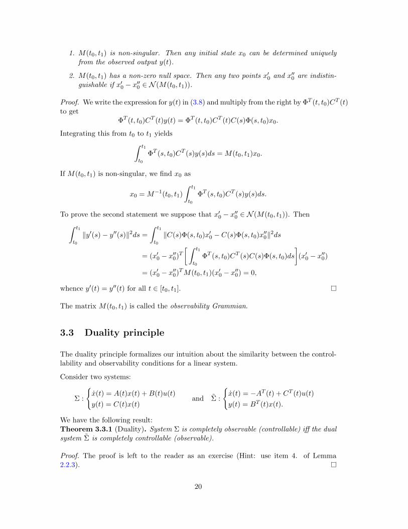
1. M(t0, t1) is non-singular. Then any initial state x0 can be determined uniquelyfrom the observed output y(t).
2. M(t0, t1) has a non-zero null space. Then any two points x′0 and x′′0 are indistin-guishable if x′0 − x′′0 ∈ N (M(t0, t1)).
Proof. We write the expression for y(t) in (3.8) and multiply from the right by ΦT (t, t0)CT (t)to get
ΦT (t, t0)CT (t)y(t) = ΦT (t, t0)CT (t)C(s)Φ(s, t0)x0.
Integrating this from t0 to t1 yields∫ t1
t0
ΦT (s, t0)CT (s)y(s)ds = M(t0, t1)x0.
If M(t0, t1) is non-singular, we find x0 as
x0 = M−1(t0, t1)
∫ t1
t0
ΦT (s, t0)CT (s)y(s)ds.
To prove the second statement we suppose that x′0 − x′′0 ∈ N (M(t0, t1)). Then∫ t1
t0
‖y′(s)− y′′(s)‖2ds =
∫ t1
t0
‖C(s)Φ(s, t0)x′0 − C(s)Φ(s, t0)x′′0‖2ds
= (x′0 − x′′0)T[ ∫ t1
t0
ΦT (s, t0)CT (s)C(s)Φ(s, t0)ds
](x′0 − x′′0)
= (x′0 − x′′0)TM(t0, t1)(x′0 − x′′0) = 0,
whence y′(t) = y′′(t) for all t ∈ [t0, t1].
The matrix M(t0, t1) is called the observability Grammian.
3.3 Duality principle
The duality principle formalizes our intuition about the similarity between the control-lability and observability conditions for a linear system.
Consider two systems:
Σ :
x(t) = A(t)x(t) +B(t)u(t)
y(t) = C(t)x(t)and Σ :
x(t) = −AT (t) + CT (t)u(t)
y(t) = BT (t)x(t).
We have the following result:Theorem 3.3.1 (Duality). System Σ is completely observable (controllable) iff the dualsystem Σ is completely controllable (observable).
Proof. The proof is left to the reader as an exercise (Hint: use item 4. of Lemma2.2.3).
20

3.4 Controllability of an LTI system
From now on we will consider LTI systems, that is linear systems with constant coeffi-cients:
x(t) = Ax(t) +Bu(t), x(t0) = x0,y(t) = Cx(t),
(3.11)
where A, B and C are matrices of appropriate dimensions. For the system (3.11) thecontrollability Grammian turns out to be
W (t) =
∫ t
0eA(t−s)B(s)BT (s)eA
T (t−s)ds. (3.12)
Exercise 3.4.1. Show that the transpose operation and the matrix exponentiationcommute.
3.4.1 Kalman’s controllability criterion
Theorem 3.4.1. The system (3.11) is completely controllable iff
rank[B AB A2B . . . An−1B
]= n. (3.13)
Proof. (⇒): Let the system (3.11) be completely controllable. Assume that
rank[B AB A2B . . . An−1B
]= m < n.
Then there exists a non-zero vector c such that
cT[B AB A2B . . . An−1B
]= 0
which is equivalent to cTB = 0, cTAB = 0,. . . , cTAn−1B = 0. By the Cayley-Hamiltontheorem this implies that cTAkB = 0 for all k ≥ 0 and hence
cT eAtB = 0 ∀t ≥ 0.
This implies that c belongs to the null space of W (t) and so, since c 6= 0, rankW (t) <n. Finally, this means that the system (3.11) is not completely controllable whichcontradicts the assumption.
(⇐): Let rank[B AB A2B . . . An−1B
]= n. Assume that the system is not con-
trollable, i.e., rankW (t) < n. Then there exists a non-zero vector c such that W (t)c = 0,which implies that cT eAtB = 0. Expanding the matrix exponential we get cTAiB = 0for all i ≥ 0. However, this implies that
rank[B AB A2B . . . An−1B
]< n,
which contradicts the assumption.
21

The matrix KC =[B AB A2B . . . An−1B
]is called the Kalman’s controllability
matrix.
The following proposition provides some intuition to the controllability criterion formu-lated above. First, we recall that a linear subspace S ⊂ Rn is invariant under the actionof A (A-invariant), where A is an [n × n]-matrix, if x ∈ S ⇒ Ax ∈ S. We have thefollowing:Proposition 3.4.2. Let S ⊂ Rn be an invariant subspace of A and let rankB = m < n.Then
det[B AB A2B . . . An−1B
]6= 0
if and only if B /∈ S.
Proof. The proof is left to the reader as an exercise.
Consider two examples.
Example 3.4.2. Let A =
[0 10 −1
]and B =
[10
]. The matrix exponential is eAt =[
1 e−t
0 1− e−t]
and the controllability Grammian is W (t) =t∫
0
[1 00 0
]dτ . Note that
rankW (t) = 1 for any t > 0.
Example 3.4.3. Let A =
[0 1−1 0
]and B =
[10
]. The matrix exponential is eAt =[
cos(t) sin(t)− sin(t) cos(t)
]and the controllability Grammian is
W (t) =
t∫0
[cos2(t) − cos(t) sin(t)
− cos(t) sin(t) sin2(t)
]dτ =
1
4
[2t+ sin (2 t) −2 sin2(t)
−2 sin2(t) 2t− sin (2 t)
].
One can easily check that detW (t) = 14
(t2 − sin2(t)
)6= 0 for any t > 0.
The above illustrates the following important fact.
For an LTI system the property of being completely controllable does not dependon the considered time interval [0, T ].
3.4.2 Decomposition of a non-controllable LTI system
This subsection continues developing geometrical intuition about the controllabilityproperty of an LTI system which we briefly touched upon in Prop. 3.4.2.
Let us again consider an [n × n] matrix A and its invariant subspace S. Then thereexists a complementary subspace S such that S ⊕ S = Rn.
Let the system (3.11) fails to be completely controllable, i.e.,
rank[B AB A2B . . . An−1B
]= m < n.
22

This means that the controllability matrix KC has exactly m independent columns.Consider the linear subspace generated by these columns: S = span(KC). Then wehave the following result.Lemma 3.4.3. Subspace S = span(KC) is A-invariant.
Proof. Consider
AS = span(AKC) = span[AB A2B A3B . . . AnB
].
The columns of first n − 1 components of the matrix AKC belong to S. To show thatthe columns of AnB also belong to S we use the Cayley-Hamilton theorem and writeAnB as
AnB = −(anI + an−1A+ . . .+ a1An−1)B,
whence follows that the columns of AnB are linear combinations of vectors from S.Thus we have AS ⊆ S.
Let vectors (v1, v2, . . . vm) form a basis of S. Consider a matrix T =[v1 v2 . . . vm T
],
where T is chosen such that T is non-singular.Lemma 3.4.4. The matrix T defines a transformation such that the matrices A and Btake the following form:
AC = T−1AT =
[A11 A12
0 A22
], BC = T−1B =
[B1
0
]. (3.14)
Proof. First, we show that AT = TAC . Let us rewrite this as follows:
A[v1 v2 . . . vm | T
]=[v1 v2 . . . vm | T
] [A11 A12
0 A22
].
The vectors vi are A-invariant, thus the product A[v1 v2 . . . vm
]can be written as
a linear combination of the same vectors vi. This implies that the matrix A21 = 0.
For BC , we need to check that B = TBC . This follows from the fact that span (B) ⊂S.
3.4.3 Hautus’ controllability criterion
An alternative way to check the controllability of an LTI system is given by Hautus’controllability condition as detailed below.Theorem 3.4.5. The system (3.11) is completely controllable if and only if
rank(sI −A,B) = n for all s ∈ C. (3.15)
Proof. (⇒): Assume that there exists an s0 ∈ C such that rank(s0I −A,B) < n. Thenthere exists a non-zero vector c for which
cT (s0I −A,B) = 0 ⇒ cTA = s0cT and cTB = 0.
23

From the last equalities we have cTAkB = sk0cTB = 0 for all k ≥ 1, which implies that
cT[B AB . . . AkB
]= 0. Hence, (3.11) is not completely controllable.
(⇐): Assume that the system (3.11) is not completely controllable. This implies thatthe controllability subspace S = span(C) has dimension less than n, i.e., dimS < n.Let S⊥ be the orthogonal complement of S, i.e., for any v ∈ S and w ∈ S⊥ we havevTw = 0. We can observe that S⊥ is AT -invariant, i.e., ATS⊥ ⊆ S⊥ as folows fromvTATw = (Av)Tw=0. The latter equality follows from the fact that S is A-invariant,whence Av ∈ S.
It is known that every invariant subspace contains at least one eigenvector s, i.e., thereexist λ ∈ C and s ∈ S⊥ such that AT s = λs or, equivalently, sT (A− λI) = 0. However,we also have sTB = 0 for any s ∈ S⊥. Thus (3.15) does not hold.
Remark. Note that the Hautus condition can be simplified even further by requiringthat (3.15) holds for all s ∈ Λ(A) as for s /∈ Λ(A) we have rank(SI −A) = n and (3.15)is satisfied trivially.
3.5 Observability of an LTI system
The observability conditions can be derived from controllability conditions by using theduality principle. In particular, we have the following counterparts of the Kalman andHautus controllability criteria discussed in the previous section.
Theorem 3.5.1 (Kalman’s observability criterion). The system (3.11) is completelyobservable iff
rank
CCA· · ·
CAn−1
= n. (3.16)
Proof. We recall that the observability of (3.11) is equivalent to the controllability ofx(t) = −AT (t) + CT (t)u(t)
y(t) = BT (t)x(t).
Thus we write the observability condition
rank[CT −ATCT · · · (−AT )n−1CT
]= rank
CCA· · ·
CAn−1
= n.
Note that the rank of a matrix is invariant under transposition and elementary rowoperations (row switching, multiplication, addition).
The matrix KO =
CCA· · ·
CAn−1
will be referred to as the Kalman’s observability matrix.
24

Theorem 3.5.2 (Hautus’ observability criterion). The system (3.11) is completely ob-servable if and only if
rank
[sI −AC
]= n for all s ∈ C. (3.17)
Proof. Using the duality principle we write
rank[sI +AT CT
]= rank
[sI −AC
]= n for all s ∈ C. (3.18)
In the first equality we transposed the fist matrix, multiplied the first n rows by −1 andused the fact that s is arbitrary.
3.5.1 Decomposition of a non-observable LTI system
Similarly to the decomposition into controllable and uncontrollable subsystems, a non-observable linear time-invariant system can be decomposed into an observable and un-observable subsystem as stated below.
Consider an uncontrollable LTI system, i.e., the system (3.11) such that dimKO =m < n. Let vectors wT1 , w
T2 , . . . w
Tm form a basis of span(KT
O). Consider a matrix
T =[wT1 wT2 . . . wTm T
]T, where T is chosen such that T is non-singular.
Lemma 3.5.3. The matrix T defines a transformation such that the matrices A and Btake the following form:
AO = TAT−1 =
[A11 0A21 A22
], CO = CT−1 =
[C1 0
].
Proof. To prove this Lemma we first show that span(KTO) is AT -invariant. Next, we
show that1 ATT T = T T (AO)T which is equivalent to
AT[wT1 wT2 . . . wTm T
]=[wT1 wT2 . . . wTm T
] [AT11 AT21
0 AT22
].
The rest is left to the reader as an exercise.
3.6 Canonical decomposition of an LTI control system
Consider a general linear control system (3.11) such that rankKC = k1 ≤ n andrankKO = k2 ≤ n. The vector space Rn can be decomposed in two ways: as adirect sum of the controllable and uncontrollable subspaces, Rn = C ⊕ C⊥, whereC = span(KC), dim C = k1 or as a direct sum of the observable and unobservable
1This a little messy notation is the price that we have to pay for staying with columns and columnspaces.
25

subspaces, Rn = O ⊕O⊥, where O = span(KO), dimO = k2. Note that some of thesesubspaces can be trivial.
Without going into too much detail we formulate the following result.Theorem 3.6.1. There exists a non-singular [n× n]-matrix T such that
A = T−1AT =
A11 0 A13 0A21 A22 A23 A24
0 0 A33 00 0 A43 A44
, B = T−1B =
B1
B2
00
,C = CT =
[C1 0 C3 0
].
(3.19)
The transformed system is composed of four subsystems:
• (A11, B1, C1) – controllable, observable;
• (A22, B2, 0) – controllable, unobservable;
• (A33, 0, C3) – uncontrollable, observable;
• (A44, 0, 0) – uncontrollable and unobservable.
Note that these subsystems are not fully decoupled as the off-diagonal matrices A13, A21
etc. can be non-zero. However, when studying structural properties of the system wecan neglect these coupling erms as they do not influence the controllability/observabilityproperties. Note that the second block-column of A is all zero except A22; the third rowis all zero except A33.Exercise 3.6.1. Explain why the subsystem (A44, 0, 0) is uncontrollable and unobserv-able despite A24 6= 0 and A42 6= 0.
26

Chapter 4
Stability of LTI systems
4.1 Matrix norm and related inequalities
A vector space X is said to be normed if for any x ∈ X there exists a nonnegativenumber ‖x‖ which is called a norm and which satisfies the following conditions:
1. ‖x‖ ≥ 0 and ‖x‖ = 0⇔ x = 0,
2. ‖ax‖ = |a|‖x‖ for any x ∈ X and a ∈ R,
3. ‖x+ y‖ ≤ ‖x‖+ ‖y‖ (triangle inequality).
In the following we will consider X = Rn and will use the Euclidean norm ‖x‖ =√n∑i=1
x2i .
Note that all presented results remain valid if we consider X = Cn with a change of theEuclidean norm to the Hermitian one.
For any Q ∈ Rm×n, the Euclidean norm induces a matrix norm (A.K.A. spectral norm)
‖Q‖ = maxx 6=0
‖Qx‖‖x‖
= max‖x‖=1
‖Qx‖ = max‖x‖=1
√xTQTQx.
Consider the matrix QTQ. This matrix is nonnegative and symmetric. Thus all itseigenvalues are nonnegative and real. The square roots of the respective eigenvalues arecalled the singular values of the matrix Q.Lemma 4.1.1. If Q ∈ Rm×n, then ‖Q‖ = ‖QT ‖ =
√λn, where λn is the largest
eigenvalue of QTQ. Also, λn is equal to the largest eigenvalue of QQT .
Proof. First, we consider the following optimization problem:
µ2 = maxxT x=1
xTQTQx. (4.1)
27

The corresponding Lagrange function is L(x, λ) = xTQTQx + λ(1 − xTx) and thenecessary optimality conditions are
∂L
∂x= 2QTQx− 2λx = 0,
∂L
∂λ= 1− xTx = 0.
We see that the extremal value of x, denoted by x∗ is such that x∗ 6= 0. The firstequation implies that x∗ is an eigenvector of QTQ and λ is the corresponding eigenvalue.Substituting x∗ into (4.1) we get
µ2 = maxxT x=1
xTQTQx = max(x∗)T x∗=1
x∗QTQx∗ = max(x∗)T x∗=1
λ(x∗)Tx∗ = λn,
whence µ =√λn.
Next, we observe that if λ is a nonzero eigenvalue of QTQ then it is also an eigenvalue ofQQT . IfQTQx = λx thenQQT (Qx) = λ(Qx). Thus we conclude that ‖Q‖ = ‖QT ‖.
Lemma 4.1.2. If matrix Q is block-diagonal, i.e.,
Q =
Q1 0 0
0. . . 0
0 0 Qk
,we have ‖Q‖ = max
i=1,...,k‖Qi‖.
Proof. We note that
QTQ =
QT1 Q1 0 0
0. . . 0
0 0 QTkQk
and so, µ = max
λ∈Λ(QTQ)
√λ = max
i=1,...,kmax
λi∈Λ(QTi Qi)
√λi = max
i=1,...,k‖Qi‖.
Basic properties of the induced matrix norm. If A and B are real matrices then
1. ‖A‖ ≥ 0 and ‖A‖ = 0⇔ A = 0,
2. ‖aA‖ = |a|‖A‖ for any a ∈ R,
3. ‖A+B‖ ≤ ‖A‖+ ‖B‖,
4. ‖Ax‖ ≤ ‖A‖ · ‖x‖,
5. ‖AB‖ ≤ ‖A‖ · ‖B‖,
6. ‖A‖ = ‖AT ‖.
To prove the 4-th and the 5-th properties we will use the definition of the spectral norm:
‖A‖ = maxx 6=0
‖Ax‖‖x‖
⇒ ‖A‖ ≥ ‖Ax‖‖x‖
⇒ ‖A‖ · ‖x‖ ≥ ‖Ax‖
‖AB‖ = maxx 6=0
‖ABx‖‖x‖
= maxx 6=0
‖Ay‖‖y‖
·‖Bx‖‖x‖
≤ maxy 6=0
‖Ay‖‖y‖
·maxx 6=0
‖Bx‖‖x‖
⇒ ‖AB‖ ≤ ‖A‖·‖B‖,
where in the last construction we denoted y = Bx.
28
Matrix exponential and its estimates. Let A ∈ Rn×n. Consider the matrix expo-nential eAt. We have the following results.Lemma 4.1.3. ‖eAt‖ ≤ e‖A‖·|t| for all t ≥ 0.
Proof. Using the properties of the induced matrix norm we have:
‖eAt‖ ≤∞∑i=0
∣∣∣∣ tii!∣∣∣∣ ‖Ai‖ ≤ ∞∑
i=0
|t|i
i!‖A‖i ≤ e‖A‖·|t|.
Theorem 4.1.4. Given an [n × n] real matrix A, let α = maxλ∈Λ(A)
<(λ). Then for any
ε > 0 there exists γ(ε) ≥ 1 such that for any t ≥ 0 holds
‖eAt‖ ≤ γ(ε)e(α+ε)t.
Proof. The proof is based on the fact that any square matrix A can be transformedto a Jordan (block-diagonal) form by a similarity transformation: A = PJP−1. Itfollows that eAt = PeJtP−1 and hence, ‖eAt‖ ≤ ‖P‖ · ‖eJt‖ · ‖P−1‖. The proof isconcluded by considering the norms ‖eJit‖, where Ji are the elementary blocks of theJordan matrix.
4.2 Stability of an LTI system
4.2.1 Basic notions
In this and the subsequent sections we will consider the stability property of an uncon-trolled LTI system. That is to say, we will set u = 0 and will consider the homogeneoussystem
x(t) = Ax(t), x(0) = x0. (4.2)
Definition 4.2.1. An LTI system (4.2) is said to be uniformly stable if for any x0 thereexists a constant γ ≥ 1 such that the respective solution x(t, x0) to the system (4.2)satisfies
‖x(t, x0)‖ ≤ γ‖x0‖
for any t ≥ 0.Definition 4.2.2. An LTI system (4.2) is said to be exponentially stable if for any x0
there exist constants γ ≥ 1 and σ > 0 such that the respective solution x(t, x0) to thesystem (4.2) satisfies
‖x(t, x0)‖ ≤ γe−σt‖x0‖
for any t ≥ 0.Theorem 4.2.1. System (4.2) is exponentially stable iff all eigenvalues of A havestrictly negative real parts.
29
Proof. (⇒): Suppose that there exists an eigenvalue λ ∈ Λ(A) such that <(λ) ≥ 0. Let vbe the corresponding eigenvector, then the system has a particular solution x(t) = eλtv.The norm of x(t) does not decrease to 0 with time, thus the system is not asymptoticallystable.
(⇐): Suppose that all eigenvalues of (4.2) lie in the open left half plane of the complexplane and α is the real part of the rightmost eigenvalue. Let ε > 0 be a sufficientlysmall positive constant s.t. α + ε < 0. Then according to Theorem 4.1.4 we have‖eAt‖ ≤ γe(α+ε)t and so,
‖x(t, x0)‖ ≤ ‖eAt‖ · ‖x0‖ ≤ γe(α+ε)t‖x0‖.
Corollary 4.2.2. System (4.2) is exponentially stable iff all roots of the characteristicpolynomial det(sI−A) = sn+a1s
n−1 + . . .+an−1s+an have strictly negative real parts.Such polynomials are said to be Hurwitz stable.
4.2.2 * Some more about stability
Multiple eigenvalues. To warm up for this little excursion, the reader is asked toprove the following standard result.
Exercise 4.2.1. Show that if for the matrix A
• λ is a real eigenvalue with eigenvector v, then there is a solution to the system(4.2) of the form x(t) = veλt.
• λ = a ± ib is a complex conjugate pair with eigenvectors v = u ± iw (whereu,w ∈ R) then x1(t) = eat(u cos bt − w sin bt) and x2(t) = eat(u sin bt + w cos bt)are two linearly-independent solutions.
We can thus observe that the real part of λ is the key ingredient in determining stability(as we already mentioned in the preceding section). However, there are some exceptions.
When multiple eigenvalues exist and there are not enough linearly-independent eigen-vectors to span Rn, the solutions behave like |x(t)| ∼ tke<(λ)t , where (k − 1) does notexceed the algebraic multiplicity of the root λ. This implies that a solution can havea large overshoot, but it will eventually decay if λ < 0. Note that an overshoot mayoccur even for simple eigenvalues.
Example 4.2.2. Consider the system (4.2) with the matrix A =
[−2 α0 −1
]. Its eigen-
values are −1 and −2, and the respective eigenvalues are v1 =
[10
]and v2 =
[α1
].
The eigenvalues are real negative, hence the system is stable. However, taking x(0) =v2 − αv1, the first coordinate x1(t) = α(e−t − e−2t) initially grows from zero to a maxi-mum value of α/4 at t = − ln(1/2). For sufficiently large α, the trajectory first movesfar away from the fixed point before approaching it as t→∞.
Finally, consider the matrix A such that there is one eigenvalue λ, <(λ) = 0, of multi-plicity greater than 1. Two cases are possible:
30

1. The geometric multiplicity of λ is less than its algebraic multiplicity, i.e., theeigenvalues associated with λ form a linear subspace of dimension less than thealgebraic multiplicity of λ. Then, there exists a vector v (called the generalizedeigenvector) such that the respective solution will be of form x(t) = vt (dependingon the difference between the algebraic and the geometric multiplicities there couldbe terms involving tk with k > 1).
2. If the geometric and the algebraic multiplicities of λ coincide, that is λ is asemisimple eigenvalue, the matrix A can be transformed to a diagonal one andhence all solutions either will be constants or will oscillate with constant amplitudedepending on the imaginary part od λ.
The former solution is unstable, while the latter one is uniformly stable (but obviouslynot exponentially stable).
Stability of time-variant systems. In our course we do not consider stability oftime-variant systems. In general, LTV systems behave similar to LTI ones, but somemore caution is needed when defining the exponential stability property as the followingexample demonstrates.
Example 4.2.3. Consider the system x = −xe−t. It satisfies the condition of Definition4.2.2 with γ = 1. However, the system does not converge to x(t) = 0 as t→∞ since theright-hand side decreases faster than exponentially and hence x(t) converges to somefinite non-zero value 0 < x∗ < x(t0).
To overcome this difficulty we may extend Definition 4.2.2 by requiring that there existconstants γl < γ and σl > σ such that
γle−σlt‖x0‖ ≤ ‖x(t; t0, x0)‖ ≤ γe−σt‖x0‖.
The left inequality effectively prevents x(t; t0, x0) from decreasing faster than exponen-tially.
4.2.3 Lyapunov’s criterion of asymptotic stability
Definition 4.2.3. A quadratic form v(x) = xTV x, V = V T , is said to be positivedefinite (positive semi-definite) if v(x) > 0 (v(x) ≥ 0) for any x ∈ Rn \ 0.
Since V = V T , all eigenvalues of V are real. Furthermore, a quadratic form is positivedefinite if and only if all its eigenvalues are strictly positive. This follows, for instance,from the following estimate:
λmin‖x‖2 ≤ v(x) ≤ λmax‖x‖2.
We have the following result.Theorem 4.2.3. The system (4.2) is exponentially stable if and only if there existtwo positive definite quadratic forms v(x) = xTV x and w(x) = xTWx such that thefollowing identity holds along the solutions of (4.2):
d
dtv(x(t)) = −w(x(t)). (4.3)
31

The quadratic form v(x) satisfying (4.3) is called the quadratic Lyapunov function.
Proof. Necessity: Let the system (4.2) be exponentially stable. We choose a positivedefinite quadratic form w(x) = xTWx and show that there exists a positive definitequadratic form v(x) s.t. (4.3) holds.
Integrating (4.3) from t = 0 to t = T we get
v(x(T, x0))− v(x(0, x0)) = −∫ T
0w(x(t, x0))dt.
Since the system is exponentially stable we have limT→∞
x(T ) = 0 and so, limT→∞
v(x(T )) =
0. Thus,
v(x0) =
∫ ∞0
w(x(t, x0))dt =
∫ ∞0
xT0 eAT tWeAtx0 dt.
The last integral converges as w(x(t, x0)) ≤ λmax(W )γ2e−2σt‖x0‖2, t ≥ 0. Furthermore,this integral is a quadratic form in x0 with
V =
∫ ∞0
eAT tWeAt dt.
Positive definiteness of V follows from the estimate xT (t, x0)Wx(t, x0) ≥ λmin(W )‖x(t, x0)‖2,which implies that
v(x0) =
∫ ∞0
xT (t, x0)Wx(t, x0)dt ≥ λmin(W )
∫ ∞0‖xT (t, x0)‖2dt.
Sufficiency: Let σ > 0 be such that for any x ∈ Rn 2σv(x) ≤ w(x). In particular, we
can choose σ = λmin(W )2λmax(V ) . Then we can write
d
dtv(x(t)) = −w(x(t)) ≤ −2σv(x(t)), t ≥ 0.
This inequality implies that
v(x(t)) ≤ e−2σtv(x0),
and hence,
λmin(V )‖x(t, x0)‖2 ≤ v(x(t, x0)) ≤ e−2σtv(x0) ≤ λmax(V )e−2σt‖x0‖2.
The above can be rewritten to yield an exponential estimate on the solution of (4.2):
‖x(t, x0)‖ ≤ γe−σt‖x0‖,
where γ =√
λmax(V )λmin(V ) and σ is as defined above.
32
4.2.4 Algebraic Lyapunov matrix equation
Let v(x(t)) = xT (t)V x(t) be a quadratic form. We write explicitly the derivativeddtv(x(t)) taken in virtue of (4.2):
d
dt
(xTV x
)= xTV x+ xTV x = xTATV x+ xTV Ax = xT (ATV + V A)x.
Checking condition (4.3) of Theorem 4.2.3 thus boils down to solving the followingalgebraic Lyapunov matrix equation:
ATV + V A = −W. (4.4)
Theorem 4.2.4. The algebraic Lyapunov matrix equation (4.4) has a unique solutioniff the spectrum of the matrix A does not contain an eigenvalue s0 such that −s0 alsobelongs to the spectrum of A.
Proof. Necessity: Let there exists s0 ∈ Λ(A) such that −s0 ∈ Λ(A). Then there existtwo non-zero vectors b and c such that bA = s0b and cA = −s0c. This implies that thehomogeneous equation ATV + V A = 0 has a non-zero solution given by V = cT b. Thiscontradicts the consistency condition – add details
We will refer to the condition above (given A, @s0 ∈ C s.t. s0 ∈ Λ(A) and −s0 ∈ Λ(A))as the Lyapunov condition.Corollary 4.2.5. Let the matrix A satisfy the Lyapunov condition. Then for anysymmetric W the unique solution of (4.4) is also a symmetric matrix.Corollary 4.2.6. If the matrix W is positive definite and all eigenvalues of A lie inthe open left half plane of C, then the corresponding matrix V is also positive definite.Lemma 4.2.7. Let the system (3.11) be observable (controllable). The matrix A haseigenvalues in the open left half plane of C if and only if the Lyapunov matrix equation
ATV + V A = −CTC
for the observable case, or
ATV + V A = −BBT
for the controllable case has a unique positive definite solution V .
4.3 Hurwitz stable polynomials
In this section we will study characteristic polynomials
p(s) = det(sI −A) = sn + a1sn−1 + . . .+ an−1s+ an, (4.5)
where s ∈ C and ai ∈ R, i = 1, . . . , n.Definition 4.3.1. The polynomial p(s) is said to be Hurwitz stable if all roots of p(s)have strictly negative real parts.
33

4.3.1 Stodola’s necessary condition
Theorem 4.3.1. Let polynomial p(s) be Hurwitz stable, then all coefficients ai arestrictly positive.
4.3.2 Hurwitz stability criterion
Consider the polynomial (4.5), the [n× n] matrix
H =
a1 a3 a5 . . . 0 0
1 a2 a4...
...
0 a1 a3. . .
......
......
... an−1 00 0 0 . . . an−2 an
is called the Hurwitz matrix corresponding to the polynomial p.Theorem 4.3.2. A real polynomial is Hurwitz stable polynomial if and only if all theleading principal minors of the matrix H(p) are positive.Example 4.3.1. Consider a polynomial of degree 3: p(s) = s3 + a1s
2 + a2s+ a3. Thispolynomial is Hurwitz stable if
∆1(p) =∣∣a1
∣∣ = a1 > 0
∆2(p) =
∣∣∣∣a1 a3
a0 a2
∣∣∣∣ = a2a1 − a0a3 > 0
∆3(p) =
∣∣∣∣∣∣a1 a3 a5
a0 a2 a4
0 a1 a3
∣∣∣∣∣∣ = a3∆2 − a1(a1a4 − a0a5) > 0
4.4 Frequency domain stability criteria
The frequency based stability analysis is based upon the use of the argument principle.Before we proceed to the main results we note that in contrast to the classical complexanalysis where one uses the principal value, i.e., a multivalued function Arg(s) definedin (−π, π], we will employ a more general notion of argument. Namely, we will assumethat along any parametrized curve a(ω) ∈ C, ω ∈ (−∞,∞) the argument functionarg(a(ω)) is a single valued and continuous function of ω. Note also that we will use inthe following the terms argument and phase, resp. change of argument and phase shiftinterchangeably.Theorem 4.4.1 (Cauchy). If f(s) is a meromorphic function defined on the closure ofa simply connected open set S, and f(s) has no zeros or poles on the boundary ∂S, then
N − P =1
2πi
∮∂S
df
f=
1
2π∆∂S arg[f(s)]
34
where N and P denote the number of zeros and poles of f(s) on the set S, with eachzero and pole counted taking into account their multiplicity and order, respectively;∆∂S arg[f(s)] is the net change of the argument of f(s) as s traverses the contour∂S in the counterclockwise direction.
Since we wish to distinguish between the “left” and the “right” roots of the characteristicpolynomial p(s), we will concentrate on the case where f(s) = p(s) and S is chosen tobe the open left half-plane of the complex plane. The latter implies that the boundary∂S coincides with the imaginary axis. For this case, Theorem 4.4.1 can be used to provethe following result.Corollary 4.4.2. Let polynomial p(s) be of degree n and have no zeros on the imaginaryaxis, then the net change of the argument function
∆ arg[p(s)]
∣∣∣∣ j∞−j∞
= (2ν − n)π,
where ν is the number of zeros of p(s) in the left half-open plane of C.
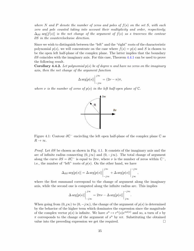
Figure 4.1: Contour ∂C− encircling the left open half-plane of the complex plane C asR→∞.
Proof. Let ∂S be chosen as shown in Fig. 4.1. It consists of the imaginary axis and thearc of infinite radius connecting (0, j∞) and (0,−j∞). The total change of argumentalong the curve ∂S = ∂C− is equal to 2πν, where ν is the number of zeros within C−,i.e., the number of “left” roots of p(s). On the other hand, we have
∆∂S arg[p(s)] = ∆ arg[p(s)]
∣∣∣∣ j∞−j∞
+ ∆ arg[p(s)]
∣∣∣∣−j∞j∞
,
where the first summand correspond to the change of argument along the imaginaryaxis, while the second one is computed along the infinite radius arc. This implies
∆ arg[p(s)]
∣∣∣∣ j∞−j∞
= 2πν −∆ arg[p(s)]
∣∣∣∣−j∞j∞
.
When going from (0, ∞) to (0,−j∞), the change of the argument of p(s) is determinedby the behavior of the higher term which dominates the expression since the magnitudeof the complex vector p(s) is infinite. We have sn 7→ rn(s)enφ(s) and so, a turn of s byπ corresponds to the change of the argument of sn by nπ. Substituting the obtainedvalue into the preceding expression we get the required.
35

Note that the argument principle can alternatively be formulated without resorting tothe Cauchy theorem. We formulate it as a lemma and give a different proof.Lemma 4.4.3. Let polynomial p(s) be of degree n and have no zeros on the imaginaryaxis, then the net change of the argument function
∆ arg[p(s)]
∣∣∣∣j∞0
= (2ν − n)π
2,
where ν is the number of zeros of p(s) in the left half-open plane of C.
Proof. Note that p(s) can be represented as a product of elementary polynomials:
p(s) =
k∏i=1
(s+ λi)
k+l∏j=k+1
(s+ λj)(s+ λj),
where k + 2l = n and λj denotes the complex conjugate of λj . The argument of p(s) isthe sum of arguments of the elementary polynomials. Thus it suffices to consider thesepolynomials as s changes from (0, 0) to (0, j∞) (note that we consider only the upperhalf of the imaginary axis). One can easily observe that each root with a negative realpart contributes π
2 to the total change of the argument while the contribution of anyroot with a positive real part is equivalent to −π
2 (the details are left to the reader asan exercise). Thus we have
∆ arg[p(s)]
∣∣∣∣j∞0
= νπ
2− (n− ν)
π
2= (2ν − n)
π
2.
Figure 4.2 illustrates the behavior of a real polynomial as s changes along the upperhalf of the imaginary axis. One can observe different phase shifts introduced by left andright roots. Also, Fig. 4.2d illustrates the situation where there is a pair of complexconjugate roots on the imaginary axis.
Consider now the complex plane C and an open set S ⊂ C. The set S 6= ∅, its boundary∂S and the complement of S, SC = C \ S form a partition of the complex plane, i.e.,S ∪ ∂S ∪ SC = C, S ∪ SC = ∅.
Consider the family of polynomials p(λ, s) such that
1. p(λ, s) has a fixed degree n for any λ ∈ [0, 1],
2. p(λ, s) continuously depend on λ.
This implies that we can represent this family as a monic polynomial (note that p(λ, s)is of fixed degree)
p(λ, s) = sn + a1(λ)sn−1 + · · ·+ an−1(λ)s+ an(λ),
where ai(λ), i = 1, . . . , n, are continuous functions of λ on [0, 1].Theorem 4.4.4 (Boundary crossing theorem). Let p(0, s) have all its roots in S andp(1, s) have at least one root in SC . Then, there exists at least one λ ∈ (0, 1) such that
36

(a) Λ = −1,−5,−10,−20 (b) Λ = 1, 3, 5,−15
(c) Λ = −1,−2, 7, 10 (d) Λ = −1,−5,−7j, 7j
Figure 4.2: Hodographs of a fifth degree polynomial with different sets of roots Λ. Themagnitude of the complex vectors is plotted in the logarithmic scale: rejφ 7→ log10(r) ejφ.
1. p(λ, s) has all its roots in S ∪ ∂S, and
2. p(λ, s) has at least one root on ∂S.
We return to the polynomial (4.5) and observe that it can be represented as a sum oftwo polynomials, referred to as even and odd parts:
peven(s) = a0 + a2s2 + a4s
4 + . . .
podd(s) = a1s+ a3s3 + a5s
5 + . . .(4.6)
We substitute s with jω and define
pe(w) = peven(jω) = a0 − a2ω2 + a4ω
4 − . . .
po(w) =podd(jω)
jω= a1 − a3ω
2 + a5ω4 − . . .
(4.7)
With this, we can evaluate (4.5) along the curve that coincides with the imaginary axisand is parametrized by ω:
p(ω) = (jω)n + a1(jω)n−1 + . . .+ an−1(jω) + an = pe(ω) + jω po(ω). (4.8)
37
Note that pe(ω) and po(ω) are both polynomials in ω2 and thus their roots are sym-metric with respect to the origin of C. This implies that one can consider the rootscorresponding to either the negative or the positive values of the parameter ω. We willchoose the latter.
Note also that the degree of pe is either (n− 1) or n depending on whether n is odd oreven. Respectively, the degree of po is equal to either (n− 1) or (n− 2).Definition 4.4.1. A polynomial p(ω), (4.8), satisfies the interlacing property if
1. The leading coefficients of pe(ω) and po(ω) are of the same sign, and
2. All the roots of pe(ω) and po(ω) are real, distinct, and the positive roots interlacein the following manner:
0 < ωe,1 < ωo,1 < ωe,2 < ωo,2 < . . .
Remark. Definition 4.4.1 can be alternatively formulated for peven(s) and podd(s). Inparticular, the second condition would read:
All the roots of peven(s) and podd(s) are purely imaginary, distinct, and the rootslying on the upper half of the imaginary axis interlace in the following manner:
j0 < jωe,1 < jωo,1 < jωe,2 < jωo,2 < . . .
Note that j0 is now a root of podd(s).Theorem 4.4.5 (Hermite-Biehler). A real polynomial p(s), (4.5), is Hurwitz stable ifand only if it satisfies the interlacing property.
Proof. We prove only necessity: Consider a real (monic) Hurwitz polynomial of degreen: p(s) = sn +an−1s
n−1 + · · ·+a1s+a0. According to the Stodola necessary condition,all coefficients ai of p(s) are positive. Thus, the first part of Def. 4.4.1 is satisfied.
Furthermore, we know from Lemma 4.4.3 that the phase of a stable polynomial p(jω)strictly increases from 0 to nπ/2 as ω goes from 0 to ∞. Thus the vector of p(jω)starts at (a0, j0), a0 > 0, for ω = 0 and rotates counterclockwise around the originnπ/2 radians while its amplitude strictly grows with ω. In doing so, the vector draws acurve, which crosses alternately the imaginary and the real axes as shown, e.g., in Fig.4.2a. The intersection of the imaginary axis corresponds to a root of pe(w) whereas theintersection with the real axis corresponds to a root of po(w). Therefore, the values ofω at which p(jω) crosses either the imaginary or the real axis form the sequence
0 < ωe,1 < ωo,1 < ωe,2 < ωo,2 < . . .
This concludes the first part of the proof. For more details on the Hermite-Biehlertheorem see [8] or [9].
Consider pe(ω) and po(ω). These polynomials are expressed as functions of even powersof ω. Thus we can make a substitution ω2 7→ σ that results in polynomials pe(σ) andpo(σ). The order of these polynomials is hence decreased by two.
We can now easily observe that polynomials pe(ω) and po(ω) satisfy the interlacingproperty if and only if
38

1. Their leading coefficients are of the same sign, and
2. All the roots of pe(σ) and po(σ) are real, distinct, and interlace in the followingmanner:
0 < σe,1 < σo,1 < σe,2 < σo,2 < . . .
Example 4.4.1. Consider the polynomial p(s) = s9 + 11s8 + 52s7 + 145s6 + 266s5 +331s4 + 280s3 + 155s2 + 49s + 6. The respective even and odd polynomials are thuspeven(s) = 11s8 +145s6 +331s4 +155s2 +6 and podd(s) = s8 +52s6 +266s4 +280s2 +49.Changing to ω we have pe(ω) = 11ω8−145ω6+331ω4−155ω2+6 and po(ω) = ω8−52ω6+266ω4 − 280ω2 + 49 and, finally, pe(σ) = 11σ4 − 145σ3 + 331σ2 − 155σ + 6 and po(σ) =σ4 − 52σ3 + 266σ2 − 280σ + 49. We can relatively easyly determine the roots of pe(σ)and po(σ), which are1 σe = 10.42, 2.14, 0.58, 0.04, and σo = 46.4, 4.25, 1.14, 0.22.The roots are interlacing and hence, the polynomial p(s) is Hurwitz stable.
1Rounded offto the second decimal digit.
39

Chapter 5
Linear systems in frequencydomain
5.1 Laplace transform
Consider a piecewise continuous function x(t), defined for all t ∈ [0,∞) and such thatx(t) = 0 for all t < 0. Let, furthermore, there exist positive constants M and a realnumber a such that ‖x(t)‖ < Meat when 0 ≤ t <∞.
The Laplace transform of x(t), t ∈ [0,∞), is an analytic function X(s), defined by(provided the integral converges absolutely):
X(s) =
∫ ∞0
x(t)e−st dt, (5.1)
where s is a complex (frequency) variable, s = σ + iω, with σ ∈ R and ω ∈ R. In thefollowing, we will write X(s) = Lf(t).
The set of values s for which the integral (5.1) converges absolutely is a half-planeGROC = s ∈ C|<(s) > a (<(s) ≥ a) that is referred to as the region of convergence(ROC). In particular, if x(t) is an integrable on [0,∞) function, the region of convergenceis defined as G0 = s ∈ C|<(s) ≥ 0).
The inverse Laplace transform is given by the Fourier–Mellin integral:
x(t) = L−1X(t) =1
2πilimT→∞
γ+iT∫γ−iT
estX(s) ds,
where γ > a is a real number so that the contour path of integration is in the region ofconvergence of X(s).
The Laplace transform is very similar to the Fourier transform (it can be thought asan ”analytical extension” of the FT). While the Fourier transform of a function is acomplex function of a real variable (frequency), the Laplace transform of a function is
40

a complex function of a complex variable. Laplace transforms are usually restricted tofunctions of t with t > 0. A consequence of this restriction is that the Laplace transformof a function is a holomorphic function of the variable s.Lemma 5.1.1. The Laplace transform has the following properties:
1. Lαf(t) + βg(t) = αLf(t)+ βLg(t) — linearity;
2. L ddtf(t) = sLf(t) − f(0) for any piecewise differentiable f(t);
3. L∫ t
0 f(τ)dτ = 1sLf(t) = 1
sF (s);
4. Lf(t− τ) = e−τsLf(t) = e−τsF (s);
5. F (s) ·G(s) =∫ t
0 f(τ)g(t− τ)dτ — convolution;
6. limt→0+
f(t) = lims→∞
sF (s) — initial value theorem;
7. limt→∞
f(t) = lims→0
sF (s) if all poles of sF (s) are in the left half-plane. — final value
theorem;
Proof. We will prove only the items 2) and 7). For the rest see [?].∫ ∞0
d
dτf(τ)e−sτ dτ = f(τ)e−sτ
∣∣∣∣∞0
+ s
∫ ∞0
f(τ)e−sτ dτ = −f(0) + sF (s).
To prove the final value theorem we take the limit of the above:
lims→0
[sF (s)− f(0)] = lims→0
∫ ∞0
df(t)
dte−stdt =
∫ ∞0
df(t) = f(∞)− f(0).
By canceling f(0) on both sides we arrive at
f(∞) = lims→0
[sF (s)].
5.2 Transfer matrices
The Laplace transform is particularly useful for analyzing linear dynamical systems aswill be illustrated below.
Consider the LTI system (3.11). Assume that there is a pair (M,a) such that
1. The real parts of all eigenvalues of the system matrix A are less than a;
2. The admissible input signals u(t) satisfy ‖u(t)‖ ≤Me−at for all t ≥ 0.
Then we can apply the Laplace transform to (3.11) to get (taking into account property2) of Lemma 5.1.1):
sX(s) = x(0) +AX(s) +BU(s)
Y (s) = CX(s).
41

Eliminating X(s) we arrive at
Y (s) = C(sI −A)−1BU(s) + C(sI −A)−1x(0).
The first term is the Laplace transform of the system’s output due to the input signaland the second one describes the system’s reaction to the initial conditions x(0). Whenconsidering frequency domain representation of linear control systems it is common toassume that the initial conditions are equal to zero, i.e., x(0) = 0. In this casewe can restrict ourselves to considering the input/output behavior of the control system.This approach has certain advantages as well as some drawbacks as we shall see below.
The matrix W (s) = C(sI − A)−1B relating the Laplace transform of the input andthe output signals is referred to as the transfer matrix. We can easily see that if u(t)and y(t) are scalar signals, the transfer matrix reduces to a function, which is calledthe transfer function. A transfer function can be alternatively defined as a ratio of theLaplace transforms of the output and the input functions, W (s) = Y (s)
U(s) .
5.2.1 Properties of a transfer matrix
Any entry of the transfer matrix W (s) is a rational function, given by a fraction of
two polynomials in s: Wij(s) =pij(s)qij(s)
. We will say that Wij(s) is the transfer function
between the j-th component of the output signal and the i-th component of the inputsignal.
A transfer function W (s) = p(s)q(s) is said to be proper or causal if deg(p(s)) ≤ deg(q(s))
and strictly proper (strictly causal) if this inequality is strict.
Informally, a system is causal if the output depends only on present and past, but notfuture inputs and it is strictly causal if the output depends only on past inputs.
Physically realizable transfer functions.Lemma 5.2.1. A transfer matrix is invariant w.r.t. the linear change of variables.
Proof. Consider the system (3.11) and introduce the new variables z = Tx, whereT ∈ Rn×x is non-singular. Then (3.11) turns into
x = TAT−1x+ TBu
y = CT−1x.
The respective transfer matrix is thus
W (s) = CT−1(sI − TAT−1
)−1TB
= C(sT−1IT − T−1TAT−1T
)−1B
= C (sI −A)−1B = W (s)
42

We recall the result of Theorem 3.6.1 which states that any controlled LTI system canbe decomposed into 4 subsystems. We are interested in the first one, the controllableon observable subsystem (A11, B1, C1).Theorem 5.2.2. The transfer matrix W (s) of the LTI system (3.11) coincides with thetransfer matrix of the controllable and observable subsystem of (3.11).
Proof. According to Lemma 5.2.1, the transfer matrix of the original system (3.11) andthat of its canonical decomposition (3.19) coincide. We compute the transfer matrix of(3.19) explicitly (inverse of a block matrix!):
W (s) =[C1 0 C3 0
] sI −A11 0 A13 0A21 sI −A22 A23 A24
0 0 sI −A33 00 0 A43 sI −A44
−1
B1
B2
00
=C1(sI −A11)−1B1
5.3 Transfer functions
In this Section we assume that both u(t) and y(t) are scalar signals. This allows us to
concentrate on studying a single transfer function W (s) = Y (s)U(s) . However, all results
can be easily extended to the case of vector-valued input/output functions. We beginwith giving a physical interpretation of a transfer function.
5.3.1 Physical interpretation of a transfer function
5.3.2 Bode plot
5.4 BIBO stability
43
Part II
CONTROL SYSTEMS:SYNTHESIS
44

Chapter 6
Feedback control
6.1 Introduction
In the first part of this lecture notes we studied structural properties of linear controlsystems, many of which are related to control. However, we have not addressed theproblem of control design yet (except a little digression in Sec. 3.1.1). Now we will closethis gap.
To start with, we define two fundamental classes of controls.
Definition 6.1.1. A control u(t) is said to be open-loop if it depends only on the currenttime t and closed-loop (feedback) if it depends both on the time t and the current statex(t), i.e., u(t) = u(t, x(t)).
Open-loop controls are computed off-line and stored in a look-up table. As the timegoes on, the current value of the control is computed by interpolating between the storedvalues. The control u(t) discussed in Sec. 3.1.1 is an example of open-loop control.
Closed-loop controls, in turn, are computed on-line according to a certain rule whichis referred to as the control law. It may seem that feedback control is just a specialclass of open-loop control as it reduces to u(t) when considering x(t) as a function of t.However, there is a fundamental difference: in contrast to open-loop control, feedbackcontrol can alter the system’s dynamics (for instance, an unstable system can be madestable using a feedback – a result that cannot be achieved using open-loop control).Furthermore, feedback control systms are capable of attenuating the disturbances actingon the system.
A general feedback control system is shown on Fig. 6.1. It works as follows: the measuredoutput y is transformed by the feedback controller ΣF . The difference between theresulting signal γ and the reference (or external input) signal v is the discrepancye = v − γ. The latter is transformed by the feedforward controller ΣC to yield thecontrol u which is applied to the plant Σ thus effectively closing the loop.
Two remarks are in order:
45

Figure 6.1: General structure of a feedback control system
1. Both the feedback and the feedforward controller can be either dynamic or static.In the second case, the respective controller reduces to a matrix of appropriatedimensions. In particular, any of these controllers can omitted by setting it to anidentity matrix.
2. The minus sign in the expression for the error signal reflects the common conven-tion to consider the negative feedback. However, the coefficients (gains) of thefeedback controller can be either positive or negative depending on the specificform of the control system Σ.
Note that there can be many variations of the above described scheme depending onthe problem. For instance, a feedback control system can be designed to serve as a partof another, more complex system. Thus, it is in general impossible to present a uniformcharacterization of the whole class of such systems. Instead, we shall concentrate ontwo particular cases.
6.1.1 Reference tracking control
Consider the scheme in Fig. 6.2. Here we directly prescribe how the system shouldbehave by specifying the desired system’s output y(t). The difference between thedesired and the measured outputs, e(t) = y(t) − y(t), is called the error. The errorsignal serves as the input for the controller ΣC which returns the control signal u.The control influences the system in order to minimize the absolute value of e(t) thusensuring convergence of the actual output to the desired one. The reference signal y(t)can be a constant. In this case we speak of set-point control.
Figure 6.2: A reference tracking control system
46

6.1.2 Feedback transformation
The scheme shown in Fig. 6.3 demonstrates another approach to the use of feedback.The idea consists in regarding the control u as a sum of two components, u(t) = v(t)−Σ(y(·)), where v(t) is the new control and Σ(y(·)) is a correction term that is used tomodify the dynamics of the closed-loop system. In general, ΣF (·) can be a dynamicalsystem, that is Σ(y(·)) can depend on the previous values of the system’s output y(t).However, in this notes we shall restrict ourselves to the static case.
Figure 6.3: A feedback transformation scheme
Consider our good old linear systemx(t) = Ax(t) +Bu(t),
y(t) = Cx(t),(6.1)
Let the control u(t) be defined as u(t) = v(t) − Fy(t), where F is the feedback (orfeedback gain) matrix of appropriate dimensions. With this control, (6.1) turns into
x(t) = (A−BFC)x(t) +Bv(t),
y(t) = Cx(t).(6.2)
Now, the system’s dynamics is determined by a new matrix A = (A − BFC). Notethat this has become possible because we (indirectly, through y(t)) fed the state backto the system’s input. We already know that the matrix A (precisely, its eigenvalues)determines stability of the system. Thus one may ask:
(Q1). Can one choose the matrix F to render an unstable system (6.1) stable?
It turns out that this is possible under certain conditions as will be shown in the nextSection. One might go further and ask
(Q2). Can one choose the matrix F to render an uncontrollable (unobservable) system(6.1) controllable (resp. observable)?
This answer to this question turns out to be negative as the following example demon-strates.Example 6.1.1. To check controllability of the closed-loop system (6.2) we employ theHautus criterion. First we note that(
sI −A+BFC,B)
=(sI −A,B
)( I 0FC I
).
47

The last matrix is obviously non-singular, i.e., its rank is equal to (n + m). Using theinequality
rank(AB) ≤ min(rank(A), rank(B)),
we conclude that rank(sI −A+BFC,B
)≤ rank
(sI −A,B
)≤ n. Hence, an uncon-
trollable system cannot be made controllable by a static feedback. The same result canbe obtained for the observability property.
Note that the preceding analysis was performed independently on the choice of the newcontrol v(t), which can be chosen using any available method.
We conclude this section by presenting a way to relate two simingly different approachesdescribed above. Consider the scheme shown in Fig. 6.3. Let v(t) = 0, that is we setthe new control v(t) to zero. Instad of this, we introduce the reference signal y(t) bysubtracting it from the measured output y(t) (see Fig. 6.4). That is to say, we “trick”the feedback controller by feeding it with a biased signal y(t)− y(t) instead of y(t).
Figure 6.4: A modification of the feedback transformation scheme
The control signal is thus u(t) = −F (y(t)− y(t))1 and the closed-loop system isx(t) = (A−BFC)x(t) +BFy(t),
y(t) = Cx(t),(6.3)
(sI −A+BFC,BF
)=(sI −A,B
)( I 0FC F
). (6.4)
For any nontrivial feedback matrix F the last matrix in (6.4) has rank bigger than n.Noting that rank
(sI −A,B
)≤ n we conclude that the controllability property of the
modified system (6.3) depends on controllability of the original system (6.1) while thedynamics of the new system can be modified using proper choice of F .
Finally, by rearranging the components of the scheme in Fig. 6.4 we see that it turnsinto the reference tracking feedback control system as in Fig. 6.2.
1Note the sign!
48

6.2 Pole placement procedure
Consider the following basic problem: is it always possible to chose such full-statenegative feedback
u = −Fx
that the closed-loop system x = (A − BF )x possesses some desired properties (i.e., isstable, has particular root locus etc.)? The following theorem gives a (partially) positiveanswer to this question.
Theorem 6.2.1. For a pair (A,B), a matrix F ∈ Rm×n can be chosen such that theeigenvalues of (A−BF ) are arbitrarily assigned if and only if the pair(A,B) is completelycontrollable.
Proof.
(⇒): Let the pair (A,B) be not completely controllable. This implies that there ex-ists a similarity transformation T such that the system’s matrices get the form (3.14).Applying T to (A−BF ) we get
T−1(A−BF )T =
[A11 −B1F1 A12 −B1F2
0 A22
].
The eigenvalues of the matrix A22 can not be inflluenced by any choice of F and hencecan not be assigned.
(⇐): TBA...
Let us now state formally the pole placement problem.Problem. Given a pair (A,B), let Λd = λ1, . . . , λn be the desired spectrum of theclosed loop system such that λi ∈ Λd ∩ C ⇒ λi ∈ Λd. Determine F ∈ Rm×n such thatΛ(A−BF ) = Λd.
Note that the condition on λi implies that the complex eigenvalues enter the desiredspectrum only in conjugate pairs. This follows from the fact that (A − BF ) is a real-valued matrix.
The chosen set of eigenvalues uniquely determines the respective characteristic poly-nomial pd(s) =
∏ni=1(s − λi). Thus the first, direct approach would be to write the
characteristic polynomial of (A − BF ), equate it to pd(s) and use the method of un-determined coefficients to compute the components of the feedback matrix F = fij,i = 1, . . . ,m, j = 1, . . . , n. In general, such approach requires solving a system of nalgebraic equations w.r.t. mn variables fij . This is not only a tedious task, but mayalso lead to a badly posed numerical problem. Therefore, it is in general not advesedto use this approach except for the low-dimensional cases (n,m ≤ 3).
An alternative approach is based upon transforming the matrices (A,B) to the Frobeniusnormal form as described in Sec. A.2.1. We present this approach in the form of analgorithm.
49

Step 1. Compute the transformation martrix P such that PAP−1 = AF and PB =[0 . . . 0 1
]T.
Step 2. Perform the linear transformation of coordinates z = Px. In the new coordinatesthe closed-loop system x = (A−BF )x takes the form
z =
0 1 . . . 0...
.... . .
...0 0 . . . 1−an −an−1 . . . −a1
−
0...01
[f1 f2 . . . fn] z
=
0 1 . . . 0...
.... . .
...0 0 . . . 1−an −an−1 . . . −a1
−
0 0 . . . 0
0...
. . . 00 0 . . . 0
f1 f2 . . . fn
z
Step 3. Let adi , i = 1, . . . , n do the coefficients of the desired polynomial pd(s). Then wethe coefficients of F such that the following relations hold:−an−i − f1+i = −adn−ifor i = 0, . . . , n− 1. Thus, we have
f1+i = adn−i − an−i, i = 0, . . . , n− 1.
Step 4. Coefficients fi were computed for z, now we need to perform the inverse transfor-mation to return to our initial state x:
F = FP.
6.3 Linear-quadratic regulator (LQR)
Before proceeding to the LQR, we will make a short excursus to optimal control theory.
6.3.1 Optimal control basics
When determining the feedback control law it is often desirable to find a control lawthat is optimal in some sense. To make the idea of optimality more concrete we need todefine a criterion that measures the performance (or quality, productivity, etc.) of thecontrol system. The control law which minimizes this criterion while satisfying someadditional constraints is said to be optimal.
A typical control problem consists of the following ingredients:
1. Time interval [t0, T ), where the terminal time T > t0 can be either finite orinfinite. One can also consider T to be a decision variable. In this case we speakof free time optimal control problem.
50

2. Cost functional is defined as an integral
J(x, u) =
T∫t0
f0(x(τ), u(τ), τ)dτ + F (x(T )), (6.5)
where f0 is a sufficiently regular function that may be required to satisfy someadditional restrictions (convexity, non-negativeness etc.) and F (x(T )) is the ter-minal cost which is to be evaluated at the final point x(T ). The terminal costcan be used to describe soft restrictions on the terminal point. Say, we can setF (x) = (x− x)2 thus requiring the terminal state x(T ) to be as close as possibleto x.
If we considered a free time optimal control problem, J in (6.5) would also dependon T , i.e., we had J(x, u, T ).
3. State and control constraints. For instance, one may require that the controlsignal does not exceed umax in absolute value, i.e., −umax ≤ u ≤ umax. Similarconstraints can be imposed on the state x. In general, this can be written as(u, x) ∈ Ω(x, u), where the set of admissible control and state values may dependon x and u (mixed constraints).
4. Initial and final conditions. It is common to consider the initial state x(t0)(as well as the initial time t0) to be fixed while imposing different constraints onthe terminal state x(T ). It can be left unspecified (free end point), be restrictedto a certain terminal manifold, x(T ) ∈ T (variable end point), or be fixed (fixedend point).
Furthermore, there are two types of optimal control:
1. Open loop. In this case, the optimal control uo depends only on time and theinitial position x0
2, denoted by uo(t, x0). Given an initial state x0, the open loopoptimal control is computed off-line and stored in the form of a look-up table.One obvious drawback of the open loop optimal control is that it does not takeinto account any deviations from the prescribed (optimal) trajectory that mayresult from disturbances acting on the system, model uncertainties etc.
2. Closed loop (feedback). A closed loop optimal control is a function of thecurrent state and (possibly) of the time, denoted by u∗(t, x). The feedback optimalcontrol is computed on-line according to the optimal feedback law3. Note that theopen loop optimal control can be seen as a particular case of feedback optimalcontrol, which is computed for the trajectory starting at t = 0 from x0: uo(t, x0) =u∗(t, x∗(0, x0; t)), where x∗(0, x0; t) is the trajectory corresponding to the optimalcontrol u∗ and starting from x(0) = x0.
There are two specific techniques that can be used when computing optimal controls:Pontryagin’s Maximum Principle for computing open loop optimal control and Bell-
2The latter dependence is often dropped as x0 is assumed to be fixed. One thus writes uo(t)3Which is obtained as a solution to some partial differential equation as will be elaborated below.
Note that this solution may be either analytic or numerical. In the latter case, one would need to storethe parameters of the optimal control law in a form of a look-up table.
51

man’s Dynamic Programming for computing feedback optimal control. In this notes wewill consider the latter. For more details on the Pontryagin Maximum Principle see,e.g., [6, 4] as well as the original treatment of the subject by Pontryagin, Boltyanski,Gamkrelidze and Mischenko in [7].
6.3.2 Dynamic programming
We start off by considering the following (sufficiently general) optimal control problem.Let the system’s dynamics be given by
x(t) = f(x(t), u(t), t), x(t0) = x0, (6.6)
where f : X×U×[t0,∞)→ Rn is a sufficiently smooth vector valued function, X ⊆ Rn isthe set of admissible states, U is the set of admissible control values. The cost functionalto be minimized4 is
J(x, u) =
T∫t0
f0(x(τ), u(τ))dτ + F (x(T )). (6.7)
Furthermore, we drop a hard constraint on the terminal state by letting x(T ) to be freelychosen and retain only the soft one expressed by the terminal cost function F (x(T )).
The solution of the described optimal control problem relies on the following generalprinciple that was formulated by R. Bellman and is thus referred to as Bellman’s Opti-mality Principle, [2]:
An optimal policy has the property that whatever the initial state and initialdecision are, the remaining decisions must constitute an optimal policy withregard to the state resulting from the first decision.
Let W (s, xs) be the minimal value of the cost functional (6.7) when starting at time sfrom the state x(s) = xs:
W (s, xs) = minu(τ)
τ∈[s,T )
T∫s
f0(x(τ), u(τ))dτ + F (x(T )). (6.8)
Note that W (s, xs) is defined for any admissible pair (s, xs). Obviously, the solutionx(τ) in (6.8) is understood to satisfy (6.6) with x(s) = xs.
Let σ > 0 be a sufficiently small parameter. Using the additivity property of the integralwe can rewrite (6.8) as
W (s, xs) = minu(t)
t∈[s,s+σ)
s+σ∫s
f0(x(τ), u(τ))dτ + minu(t)
t∈[s+σ,T )
T∫s+σ
f0(x(τ), u(τ))dτ + F (x(T ))
.(6.9)
4The maximization problem can be addressed in the same way with a couple of obvious modifications.
52
We observe that the last two terms in (6.9) are W (s+ σ, xs+σ):
W (s, xs) = minu(t)
t∈[s,s+σ)
s+σ∫s
f0(x(τ), u(τ))dτ +W (s+ σ, xs+σ)
. (6.10)
We note that W (s + σ, xs+σ) depends on u(τ), τ ∈ [s, s + σ) as the control u(t) overthis small interval influences the value of x(t) at t = s+ σ. But W (s, xs), in turn, doesnot depend on u as it was already maximized over the whole interval [s, T ). This wecan bring W (s, xs) into the square brackets. Next, dividing the resulting expression byσ and passing to the limit (σ → 0) we get:
0 = minu(s)∈U
[f0(x(s), u(s)) +
d
dtW (t, xt)
∣∣t=s
], (6.11)
which is referred to as the Hamilton-Jacobi-Bellman (HJB) equation.Theorem 6.3.1. Let W (t, x) be a continuously differentiable function such that
0 = minu∈U
[f0(x, u) + 〈∇xW (t, x), f(x, u)〉+
∂W (t, x)
∂t
], (6.12)
holds for any admissible pair (t, x) and W (t, x) satisfies the boundary condition
W (T, x) = F (x), ∀x ∈ X.
Let there also be a piece-wise continuous in t function u∗(t, x) that minimizes the ex-pression in square brackets in (6.12) for all t and x. Then W (t, x) is the solution of theHJB equation and the function u∗(t, x) is the optimal feedback control law.
Hence, the algorithm for determining the optimal feedback control can be described asfollows:
Step 1. Write the HJB equation (6.12).
Step 2. Determine the minimizing control u∗ as a function of t, x, and ∇xW (t, x):
u∗ = u(t, x,∇xW (t, x)).
Step 3. Substitute u(t, x,∇xW (t, x)) to (6.12) to get a first order PDE:
0 = f0(x, u(t, x,∇xW )) + 〈∇xW, f(x, u(t, x,∇xW ))〉+∂W (t, x)
∂t. (6.13)
Step 4. Find a continuously differentiable solution to (6.23) satisfying the boundary con-tition W (T, x) = F (x) (or W (T, x) = 0 if there is no terminal cost).
Step 5. Compute ∇xW (t, x) and substitute the result to u(t, x,∇xW (t, x)) to get thefeedback optimal control u∗(t, x) = u(t, x,∇xW (t, x)).
53
Note that the main pitfall is that the PDE (6.23) does not always possess a continuouslydifferentaible solution. In most cases it is impossible to decide whether such a solutionexists. It is therefore common to drop the requirement of W (t, x) being continuouslydifferentiable and to consider solutions of (6.23) in some weak sense. This leads to theso called viscous and maximin solutions. An alternative approach is to discretize (6.12)and solve it numerically. This results in a sufficiently smooth approximation of theBellman function along with its first order derivatives that are then used to computethe feedback control law. However, we will not dwell upon these topics and pass on tothe linear case.
6.3.3 Linear-quadratic optimal control problem
Finally, we have arrived at our LQR problem. It is defined as follows:
Find u∗(t, x) such that
J(t, x, u∗) = min
T∫t
[xT (τ)Qx(τ) + uT (τ)Ru(τ)
]dτ, (6.14)
where Q and R are positive-definite symmetric matrices of appropriate dimensions andx(t) evolves according to
x = Ax+Bu. (6.15)
The HJB equation for the problem (6.21), (6.15) is
0 = minu∈U
[xTQx+ uTRu+ 〈∇xW (t, x), Ax+Bu〉+
∂W (t, x)
∂t
]. (6.16)
Differentiating the expression in the square brackets w.r.t. u we get5
2uTR+∇xW (t, x)B,
whence, using the first-order extremality condition,
u∗ = −1
2R−1BT∇TxW (t, x). (6.17)
One can easily check that u∗ does indeed minimizes that expression as the respectiveHessian is equal to R which is positive definite. Thus the expression to be minimized isconvex and the minimum can be achieved.
Remark. Note, however, that a little caution is necessary because the obtained optimalcontrol can happen to be outside the set of admissible control values U !
Substitute u∗ to (6.16) to get
− ∂W (t, x)
∂t= xTQx− 1
4∇xW (t, x)BR−1BT∇TxW (t, x) +∇xW (t, x)Ax. (6.18)
The PDE (6.18) is still rather difficult to deal with. However, it is known that the Bell-man function W (t, x) for the linear-quadratic optimization problems has a particularlysimple structure.
5Here and later on we assume that the gradient is a row vector.
54
Theorem 6.3.2. The Bellman function in the linear-quadratic optimization problem(6.21), (6.15) is a quadratic form
W (t, x) = xT (t)P (t)x(t),
where P (t) is a time-dependent, positive-definite symmetric matrix such that P (T ) = 0.
Now we can rewrite (6.18) taking into account that ∇xW (t, x) = 2xTP (t):
− xT P (t)x = xTQx− xTP (t)BR−1BTP (t)x+ xTP (t)Ax+ xTAP (t)x, (6.19)
which yields the following matrix differential equation, called the differential Riccatiequation (DRE):
P (t) = P (t)BR−1BTP (t)− P (t)A−AP (t)−Q, P (T ) = 0. (6.20)
Note that this equation is to be solved backwards, which is in accordance with theBellman optimality principle.
The above described result can be further simplified using the following intuitive result.Theorem 6.3.3. If the LQ optimization problem (6.21), (6.15) is defined on a semi-infinite interval with T = ∞, the Bellman function does not depend on t and can bewritten as W (x) = xT (t)Px(t), where P is a positive-definite symmetric matrix.
That is to say, if we aim at minimizing the cost functional
J(t, x, u∗) = min
∞∫t
[xT (τ)Qx(τ) + uT (τ)Ru(τ)
]dτ, (6.21)
the problem reduces to solving an algebraic Riccati equation (ARE)
0 = PBR−1BTP − PA−AP −Q. (6.22)
The optimal feedback control is thus a linear function of the system’s state:
u∗(x) = −1
2R−1BTPx (6.23)
and K = 12R−1BTP is said to be the optimal feedback gain matrix.
Remark. Note that an ARE has two solutions: a positive-definite and a negative-definiteone.
More discussion needed...
55

Chapter 7
State observers
7.1 Full state observer
For many practical problems, the full state vector of the system cannot be determinedby observing the system’s output even though the system is observable. However, itis often desirable to know the state of the system. Such information can be used todesign a linear-quadratic regulator (Sec. 6.3) or to use the pole placement procedure(Sec. 6.2), just to mention a few.
It turns out that if a system is observable, it is possible to fully reconstruct the systemstate from its output measurements using an auxiliary system which is called the stateobserver. The idea, first proposed by David Luenberger in his doctoral thesis in 1962is quite simple. Since the structure of the system is known we can easily implementa numerical model of the system. Applying to the model the same input signal thatis applied to the physical system we get the output y(t) which differs from the actualoutput y(t), the deviation being determined by the difference in the initial states of thesystem and the model. The difference y − y can be used to compute a “correction” tothe input signal applied to the model as shown in Fig. 7.1.
Figure 7.1: A state observer.
56

The resulting equations of the state observer are thus˙x = Ax+Bu+ L(y − y)
y = Cx.(7.1)
System (7.1) can be rewritten in a compact form as
˙x = (A− LC)x+ [B,L]
[u
y
]. (7.2)
Here we can observe that both the input and the output signals now serve as the inputfor our state observer. Finally, we define the observer error e = x− x. It can be readilychecked that e(t) satisfies the equation
e = (A− LC)e.
The eigenvalues of the matrix A−LC can be chosen arbitrarily by appropriate choice ofthe observer gain L when the pair [A,C] is observable, i.e. observability condition holds.In particular, it can be made Hurwitz, so the observer error e(t)→ 0 when t→∞.
Theorem 7.1.1. For a pair (A,C), a matrix L ∈ Rn×k can be chosen such that theeigenvalues of (A−LC) are arbitrarily assigned if and only if the pair(A,C) is observable.
Proof.
We can use the approach described in Sec. 6.2 if we choose A = AT and B = CT .With this, Ae turns into (AT − KBT ) = (A − BF )T , where we denoted F = KT .Since transposition does not change the eigenvalues of a matrix, we can solve the poleplacement procedure for (A− BF ). The required matrix K ...
Example 7.1.1. Consider an LTI system with A =
0 1 00 0 10 2 −1
and C =[1 0 0
].
We wish to compute K such that Ae = A − KC has the characteristic polynomialpd(s) = s3 + d2s
2 + d1s+ d0.
Following the procedure outlined above we choose A =
0 0 01 0 20 1 −1
and B =
100
.
Matrix A can be transformed to the Frobenius normal form using the the similarity
transformation A′ = PAP−1, where P =
0 0 10 1 −11 −1 3
. With this we have A′ =0 1 00 0 10 2 −1
and B′ = PB =
001
. The feedback matrix F ′ =[d0 d1 + 2 d2 − 1
].
We should not forget that matrix F ′ was computed for the transformed state z = Px.To obtain the feedback matrix for the original state x we multiply it from the right byP : F = F ′P =
[d2 − 1 −d2 + d1 + 3 3d2 − d1 + d0 − 5
]. Finally, we obtain K by
transposing F , K = F T .
57

Discussion. Why we cannot choose the gain matrix arbitrarily? In other words,why we cannot shift the eigenvalues of the closed loop matrix (A−KC) arbitrarily farto the left?
7.2 Reduced state observer
TBA...
58

APPENDIX
59
Canonical forms of a matrix
A.1 Similarity transformation
Using a non-singular change of the coordinates z = Tx one can transform the system(3.11) to an equivalent form:
z(t) = TAT−1z(t) + TBu(t), z(t0) = Tx0,y(t) = CT−1z(t).
(A.1)
Alternatively, one can write the transformation in a different way: x = Qz to yield
z(t) = Q−1AQz(t) +Q−1Bu(t), z(t0) = Q−1x0,y(t) = CQz(t).
(A.2)
Note that these two transformations are equivalent in the sense that we can derive (A.1)from (A.2) by setting Q = T−1 and vice versa1.
Transformation A = TAT−1 (resp., A = Q−1AQ) is called a similarity transformationand matrices A and A are said to be similar.
Two similar matricies share a number of properties, most important of which are :
1. Rank;
2. Characteristic polynomial and hence, the spectrum, the determinant and thetrace2.
Similarity transformation can be used to transform the original system to a more con-venient form while preserving its main characteristics. Sometimes it is possible to usea similarity transformation to shape not only the A matrix, but also B or C.
There are many approaches to the control synthesis that proceed according the followingscheme:
1. Transform the original system to a more convenient form by using a similaritytransformation z = Tx;
2. Design a control law for the transformed system: u = u(z);
1However, some transformations can be expressed in a simpler way when using (A.1) or (A.2).2Recall that det(A) =
∏ni=1 λi and tr(A) =
∑ni=1 λi, where λi are the eigenvalues of an n-by-n
square matrix A.
60

3. Perform the inverse transformation in order to express the obtained control interms of the original states: u = u(x) = u(Tx).
Note that forgetting to perform the last step will lead to a completely wrong result!
Below we consider two particularly important canonical forms that are used in controldesign.
A.2 Frobenius companion matrix
The Frobenius companion matrix of the monic polynomial
p(s) = sn + a1sn−1 + · · ·+ an−1s+ an,
is the square matrix defined as
AF (p) =
0 1 0 . . . 00 0 1 . . . 0...
......
. . ....
0 0 0 . . . 1−an −an−1 −an−2 . . . −a1
.
The following lemma explains the choice of the name.
Lemma A.2.1. The characteristic polynomial of AF (p) is equal to p.
Proof. Consider the the set of basis row vectors ei, i = 1, . . . , n such that ei isfilled with zeros and has a single “1” on the i-th position: e1 = (1, 0, . . . , 0), e2 =(0, 1, 0, . . . , 0), etc.
We have e1AF = e2, e2AF = e3, and so on until we arrive at enAF = −∑n−1
i=0 ai+1en−i.Taking into account that ek = e1A
k−1F , k = 1, . . . , n, we can combine the preceding
equations to yield (note the shifted index): e1(AnF +∑n
j=1 ajAn−jF ) = 0. Hence we
observe that p(s) = sn+∑n
j=1 ajsn−j is the annihilating polynomial ofAF . Furthermore,
the vectors e1, e1AF ,. . . , e1An−1F are linearly independent, hence the degree of p(s) is
equal to n.
In the sense of Lemma A.2.1, the matrix AF (p) is a ”companion” of the polynomial p.Remark. There are in general 4 Frobenius companion matrices. For instance, the matrix
AF (p) =
0 0 . . . 0 −an1 0 . . . 0 −an−1
0 1 . . . 0 −an−2...
.... . .
......
0 0 . . . 1 −a1
is also a companion matrix of the polynomial p(s) as well as the transposes of AF (p)and AF (p).
61

Not every square matrix is similar to a companion matrix. In general, a square matrixis similar to a matrix made up of blocks of companion matrices. The following lemmacharacterizes those matrices that are similar to a companion matrix.
Lemma A.2.2. A is similar to the companion matrix of its characteristic polynomial ifand only if there exists a cyclic vector v in Rn for A, meaning that [v,Av,A2v, . . . , An−1v]is a basis of V .
For a linear system (3.11) with a scalar control (i.e., B is a column vector), LemmaA.2.2 implies that the matrix A is similar to a companion matrix if the pair (A,B) iscontrollable, i.e., B is a cyclic vector for A.
Below we will consider such a case (B – a column vector) and present several approachesto compute the transformation matrix which turns A into a particular companion form.For the case where B is a general form [n×m] matrix, see, e.g., [1, §3.4. Controller andobserver forms].
A.2.1 Transformation of A to AF .
Below, we will consider two approaches. Note, that B is assumed to be a column vector.
Approach 1. We need to determine such non-singular transformation matrix M thatM−1AM = AF holds. Rewrite this equation as AM = MAF and denote the columnsof M by mi: M = [m1 |m2 | . . . |mn]. Then we have
[m1 |m2 | . . . |mn]
0 1 0 . . . 00 0 1 . . . 0...
......
. . ....
0 0 0 . . . 1−an −an−1 −an−2 . . . −a1
= A[m1 |m2 | . . . |mn].
Going from right to left and equating the columns we get
mn−1 − a1mn = Amn
. . . . . . . . .
m2 − an−1mn = Am2
−anmn = Am1,
whence we can express the n− 1 first columns in terms of the last one:
mn−1 = [A+ Ia1]mn
. . . . . . . . .
m1 = [An−1 +An−2a1 + · · ·+ Ian−1]mn
0 = [An +An−1a1 + · · ·+ Ian]mn.
(A.3)
Note that the last equation holds identically due to the Cayley-Hamilton theorem.
62
The remaining degree of freedom in choice of mn can be used to shape the matrix B.For instance,we may set mn = B to get BF = M−1B = [0, . . . 0, 1]T as follows from
B = MBF = [m1 |m2 | . . . |mn]
0...01
= mn.
The transformation matrix M can now be derived recursively using (A.3).
Approach 2. Let KC be the Kalman’s controlability matrix. According to LemmaA.2.2, KC is non-singular and has an inverse. Take the last row of K−1
C and denote itby q. We have qAiB = 0 for i = 0, . . . , n− 2 and qAn−1B = 1.Exercise A.2.1. Prove the above statement.
Now define the transformation matrix P :
P =
qqA...
qAn−1
.First, we observe that
PKC =
0 0 · · · 0 10 0 · · · 1 ×...
......
......
0 1 . . . × ×1 × · · · × ×
, (A.4)
which implies that det(PKC) = det(P ) det(KC) 6= 0 and hence, det(P ) 6= 0. Thus, Pis non-singular.
Next, (A.4) implies that BF = PB =[0 0 . . . 1
](as the first column of KC is equal
to B). It remains to show that PA = AFP . We write this explicitely:0 1 0 . . . 00 0 1 . . . 0...
......
. . ....
0 0 0 . . . 1−an −an−1 −an−2 . . . −a1
qqA......
qAn−1
=
qAqA2
...
...qAn
.
One can compare the resulting matrices row-wise to see that they coincide. Whencomparing the last rows recall the Cayley-Hamilton theorem.
Remark. Note that the transformation matrix P can be also represented as P = CFC−1,
where C and CF are the Kalman’s controllability matrices for the pairs (A,B) and(AF , BF )
63

A.2.2 Transformation of A to AF .
The form AF can be readily obtained by using KC as a transformation matrix. We have
AKC = KCAF .
One can follow the same line as in the previous paragraphs and compare the left and theright parts row-wise while using the Cayley-Hamilton theorem when approaching the
last row. Furthermore, we can observe that K−1C B =
[1 0 . . . 0
]Tusing the results
of Exercise A.2.1.
A.3 Jordan form
64

Bibliography
[1] Antsaklis, Panos and Anthony N. Michel. Linear systems, Springer, 2006.
[2] Bellman, R.E. Dynamic Programming. Princeton University Press, Princeton, NJ.1957. (reprinted 2003: Dover).
[3] Brockett, Roger W. Finite dimensional linear systems, John Wiley, 1970. (reprintedin SIAM series “Classics in Applied Mathematics”, 2015)
[4] Hull, David G. Optimal control theory for applications. Springer, 2003.
[5] Kharitonov, Vladimir L. Control Theory (lecture notes). 2015.
[6] Kirk, Donald E. Optimal control theory: an introduction. Prentice-Hall, Inc., En-glewood Cliffs, New Jersey, 1970. (reprinted 2012: Dover).
[7] Pontryagin, L. S., Boltyanski, V. G., Gamkrelidze, R. W., & Mischenko, E. F.Mathematical Theory of Optimal Processes. CRC Press, 1987.
[8] Postnikov, Mikhail M. Stable polynomials, Nauka, 1981. (in Russian)
[9] Rahman, Qazi Ibadur, and Gerhard Schmeisser. Analytic theory of polynomials.Oxford University Press, 2002.
65