lecture notes on superconductivity: condensed matter and qcd
TRANSCRIPT

Lecture Notes on Superconductivity:Condensed Matter and QCD
(Lectures at the University of Barcelona, Spain, September-October 2003)
Roberto Casalbuoni∗
Department of Physics of the University of Florence,Via G. Sansone 1, 50019 Sesto Fiorentino (FI), Italy
(Dated: October 13, 2003)
Contents
I. Introduction 2A. Basic experimental facts 3B. Phenomenological models 6
1. Gorter-Casimir model 62. The London theory 73. Pippard non-local electrodynamics 94. The Ginzburg-Landau theory 10
C. Cooper pairs 111. The size of a Cooper pair 14
D. Origin of the attractive interaction 15
II. Effective theory at the Fermi surface 16A. Introduction 16B. Free fermion gas 18C. One-loop corrections 20D. Renormalization group analysis 22
III. The gap equation 23A. A toy model 23B. The BCS theory 25C. The functional approach to the gap equation 30D. The Nambu-Gor’kov equations 33E. The critical temperature 36
IV. The role of the broken gauge symmetry 39
V. Color superconductivity 43A. Hierarchies of effective lagrangians 46B. The High Density Effective Theory (HDET) 47
1. Integrating out the heavy degrees of freedom 502. The HDET in the condensed phase 52
C. The gap equation in QCD 55D. The symmetries of the superconductive phases 57
1. The CFL phase 572. The 2SC phase 633. The case of 2+1 flavors 644. Single flavor and single color 66
VI. Effective lagrangians 66A. Effective lagrangian for the CFL phase 66B. Effective lagrangian for the 2SC phase 68
VII. NGB and their parameters 70A. HDET for the CFL phase 70B. HDET for the 2SC phase 73C. Gradient expansion for the U(1) NGB in the CFL model and in the 2SC model 74
∗Electronic address: [email protected]

2
D. The parameters of the NG bosons of the CFL phase 77E. The masses of the NG bosons in the CFL phase 78
1. The role of the chemical potential for scalar fields: Bose-Einstein condensation 822. Kaon condensation 84
VIII. The dispersion law for the gluons 86A. Evaluating the bare gluon mass 86B. The parameters of the effective lagrangian for the 2SC case 87C. The gluons of the CFL phase 89
IX. Quark masses and the gap equation 92A. Phase diagram of homogeneous superconductors 95B. Dependence of the condensate on the quark masses 100
X. The LOFF phase 103A. Crystalline structures 105B. Phonons 108
XI. Astrophysical implications 110A. A brief introduction to compact stars 110B. Supernovae neutrinos and cooling of neutron stars 114C. R-mode instabilities in neutron stars and strange stars 115D. Miscellaneous results 115E. Glitches in neutron stars 116
Acknowledgments 117
A. The gap equation in the functional formalism from HDET 118
B. Some useful integrals 119
References 120
I. INTRODUCTION
Superconductivity is one of the most fascinating chapters of modern physics. It has been a continuous source ofinspiration for different realms of physics and has shown a tremendous capacity of cross-fertilization, to say nothing ofits numerous technological applications. Before giving a more accurate definition of this phenomenon let us howeverbriefly sketch the historical path leading to it. Two were the main steps in the discovery of superconductivity. Theformer was due to Kamerlingh Onnes (Kamerlingh Onnes, 1911) who discovered that the electrical resistance ofvarious metals, e. g. mercury, lead, tin and many others, disappeared when the temperature was lowered below somecritical value Tc. The actual values of Tc varied with the metal, but they were all of the order of a few K, or atmost of the order of tenths of a K. Subsequently perfect diamagnetism in superconductors was discovered (Meissnerand Ochsenfeld, 1933). This property not only implies that magnetic fields are excluded from superconductors, butalso that any field originally present in the metal is expelled from it when lowering the temperature below its criticalvalue. These two features were captured in the equations proposed by the brothers F. and H. London (London andLondon, 1935) who first realized the quantum character of the phenomenon. The decade starting in 1950 was thestage of two major theoretical breakthroughs. First, Ginzburg and Landau (GL) created a theory describing thetransition between the superconducting and the normal phases (Ginzburg and Landau, 1950). It can be noted that,when it appeared, the GL theory looked rather phenomenological and was not really appreciated in the westernliterature. Seven years later Bardeen, Cooper and Schrieffer (BCS) created the microscopic theory that bears theirname (Bardeen et al., 1957). Their theory was based on the fundamental theorem (Cooper, 1956), which states that,for a system of many electrons at small T , any weak attraction, no matter how small it is, can bind two electronstogether, forming the so called Cooper pair. Subsequently in (Gor’kov, 1959) it was realized that the GL theory wasequivalent to the BCS theory around the critical point, and this result vindicated the GL theory as a masterpiece inphysics. Furthermore Gor’kov proved that the fundamental quantities of the two theories, i.e. the BCS parametergap ∆ and the GL wavefunction ψ, were related by a proportionality constant and ψ can be thought of as the Cooperpair wavefunction in the center-of-mass frame. In a sense, the GL theory was the prototype of the modern effectivetheories; in spite of its limitation to the phase transition it has a larger field of application, as shown for example byits use in the inhomogeneous cases, when the gap is not uniform in space. Another remarkable advance in these yearswas the Abrikosov’s theory of the type II superconductors (Abrikosov, 1957), a class of superconductors allowing apenetration of the magnetic field, within certain critical values.
3
The inspiring power of superconductivity became soon evident in the field of elementary particle physics. Twopioneering papers (Nambu and Jona-Lasinio, 1961a,b) introduced the idea of generating elementary particle massesthrough the mechanism of dynamical symmetry breaking suggested by superconductivity. This idea was so fruitfulthat it eventually was a crucial ingredient of the Standard Model (SM) of the elementary particles, where the massesare generated by the formation of the Higgs condensate much in the same way as superconductivity originates fromthe presence of a gap. Furthermore, the Meissner effect, which is characterized by a penetration length, is the origin,in the elementary particle physics language, of the masses of the gauge vector bosons. These masses are nothing butthe inverse of the penetration length.
With the advent of QCD it was early realized that at high density, due to the asymptotic freedom property (Grossand Wilczek, 1973; Politzer, 1973) and to the existence of an attractive channel in the color interaction, diquarkcondensates might be formed (Bailin and Love, 1984; Barrois, 1977; Collins and Perry, 1975; Frautschi, 1978). Sincethese condensates break the color gauge symmetry, the subject took the name of color superconductivity. However,only in the last few years this has become a very active field of research; these developments are reviewed in (Alford,2001; Hong, 2001; Hsu, 2000; Nardulli, 2002; Rajagopal and Wilczek, 2001). It should also be noted that colorsuperconductivity might have implications in astrophysics because for some compact stars, e.g. pulsars, the baryondensities necessary for color superconductivity can probably be reached.
Superconductivity in metals was the stage of another breakthrough in the 1980s with the discovery of high Tc
superconductors.Finally we want to mention another development which took place in 1964 and which is of interest also in QCD. It
originates in high-field superconductors where a strong magnetic field, coupled to the spins of the conduction electrons,gives rise to a separation of the Fermi surfaces corresponding to electrons with opposite spins. If the separation istoo high the pairing is destroyed and there is a transition (first-order at small temperature) from the superconductingstate to the normal one. In two separate and contemporary papers, (Larkin and Ovchinnikov, 1964) and (Fulde andFerrell, 1964), it was shown that a new state could be formed, close to the transition line. This state that hereafterwill be called LOFF1 has the feature of exhibiting an order parameter, or a gap, which is not a constant, but has aspace variation whose typical wavelength is of the order of the inverse of the difference in the Fermi energies of thepairing electrons. The space modulation of the gap arises because the electron pair has non zero total momentum andit is a rather peculiar phenomenon that leads to the possibility of a non uniform or anisotropic ground state, breakingtranslational and rotational symmetries. It has been also conjectured that the typical inhomogeneous ground statemight have a periodic or, in other words, a crystalline structure. For this reason other names of this phenomenon areinhomogeneous or anisotropic or crystalline superconductivity.
In these lectures notes I used in particular the review papers by (Polchinski, 1993), (Rajagopal and Wilczek, 2001),(Nardulli, 2002), (Schafer, 2003) and (Casalbuoni and Nardulli, 2003). I found also the following books quite useful(Schrieffer, 1964), (Tinkham, 1995), (Ginzburg and Andryushin, 1994), (Landau et al., 1980) and (Abrikosov et al.,1963).
A. Basic experimental facts
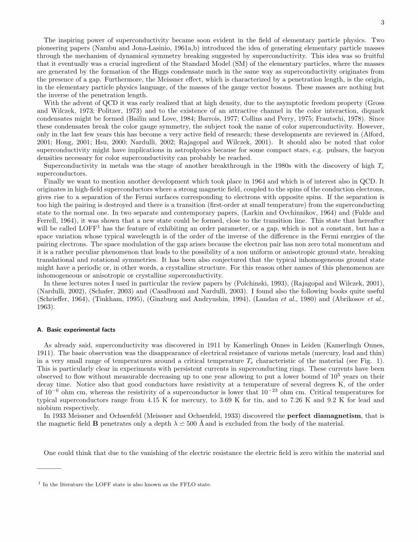
As already said, superconductivity was discovered in 1911 by Kamerlingh Onnes in Leiden (Kamerlingh Onnes,1911). The basic observation was the disappearance of electrical resistance of various metals (mercury, lead and thin)in a very small range of temperatures around a critical temperature Tc characteristic of the material (see Fig. 1).This is particularly clear in experiments with persistent currents in superconducting rings. These currents have beenobserved to flow without measurable decreasing up to one year allowing to put a lower bound of 105 years on theirdecay time. Notice also that good conductors have resistivity at a temperature of several degrees K, of the orderof 10−6 ohm cm, whereas the resistivity of a superconductor is lower that 10−23 ohm cm. Critical temperatures fortypical superconductors range from 4.15 K for mercury, to 3.69 K for tin, and to 7.26 K and 9.2 K for lead andniobium respectively.
In 1933 Meissner and Ochsenfeld (Meissner and Ochsenfeld, 1933) discovered the perfect diamagnetism, that isthe magnetic field B penetrates only a depth λ w 500 A and is excluded from the body of the material.
One could think that due to the vanishing of the electric resistance the electric field is zero within the material and
1 In the literature the LOFF state is also known as the FFLO state.
4
4.1 4.2 4.3 4.4
0.02
0.04
0.06
0.08
0.1
0.12
0.14
T(K)
ΩR( )
10-5
Ω
FIG. 1 Data from Onnes’ pioneering works. The plot shows the electric resistance of the mercury vs. temperature.
therefore, due to the Maxwell equation
∇ ∧E = −1c
∂B∂t
, (1.1)
the magnetic field is frozen, whereas it is expelled. This implies that superconductivity will be destroyed by a criticalmagnetic field Hc such that
fs(T ) +H2
c (T )8π
= fn(T ) , (1.2)
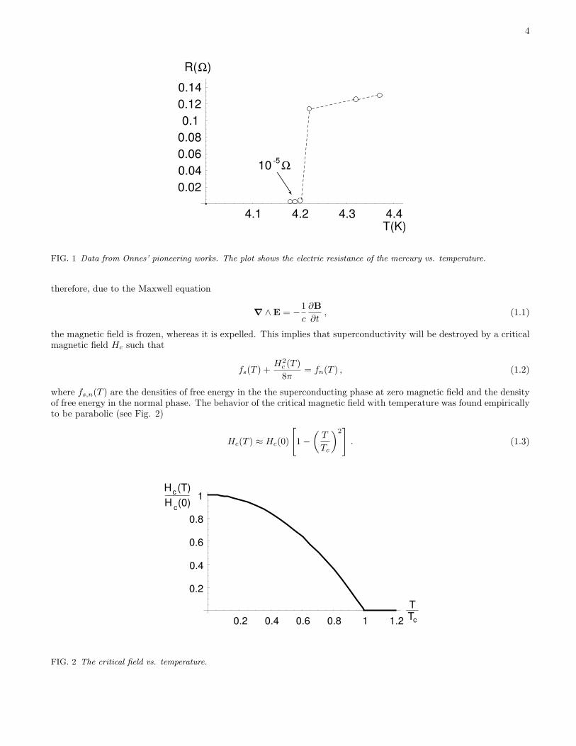
where fs,n(T ) are the densities of free energy in the the superconducting phase at zero magnetic field and the densityof free energy in the normal phase. The behavior of the critical magnetic field with temperature was found empiricallyto be parabolic (see Fig. 2)
Hc(T ) ≈ Hc(0)
[1−
(T
Tc
)2]
. (1.3)
0.2 0.4 0.6 0.8 1 1.2
0.2
0.4
0.6
0.8
1H (T)
H (0)c
c
______
TTc
___
FIG. 2 The critical field vs. temperature.

5
The critical field at zero temperature is of the order of few hundred gauss for superconductors as Al, Sn, In, Pb,etc. These superconductors are said to be ”soft”. For ”hard” superconductors as Nb3Sn superconductivity stays upto values of 105 gauss. What happens is that up to a ”lower” critical value Hc1 we have the complete Meissner effect.Above Hc1 the magnetic flux penetrates into the bulk of the material in the form of vortices (Abrikosov vortices) andthe penetration is complete at H = Hc2 > Hc1. Hc2 is called the ”upper” critical field.
At zero magnetic field a second order transition at T = Tc is observed. The jump in the specific heat is about threetimes the the electronic specific heat of the normal state. In the zero temperature limit the specific heat decreasesexponentially (due to the energy gap of the elementary excitations or quasiparticles, see later).
An interesting observation leading eventually to appreciate the role of the phonons in superconductivity (Frolich,1950), was the isotope effect. It was found (Maxwell, 1950; Reynolds et al., 1950) that the critical field at zerotemperature and the transition temperature Tc vary as
Tc ≈ Hc(0) ≈ 1Mα
, (1.4)
with the isotopic mass of the material. This makes the critical temperature and field larger for lighter isotopes. Thisshows the role of the lattice vibrations, or of the phonons. It has been found that
α ≈ 0.45÷ 0.5 (1.5)
for many superconductors, although there are several exceptions as Ru, Mo, etc.The presence of an energy gap in the spectrum of the elementary excitations has been observed directly in various
ways. For instance, through the threshold for the absorption of e.m. radiation, or through the measure of the electrontunnelling current between two films of superconducting material separated by a thin (≈ 20 A) oxide layer. In thecase of Al the experimental result is plotted in Fig. 3. The presence of an energy gap of order Tc was suggestedby Daunt and Mendelssohn (Daunt and Mendelssohn, 1946) to explain the absence of thermoelectric effects, but itwas also postulated theoretically by Ginzburg (Ginzburg, 1953) and Bardeen (Bardeen, 1956). The first experimentalevidence is due to Corak et al. (Corak et al., 1954, 1956) who measured the specific heat of a superconductor. BelowTc the specific heat has an exponential behavior
cs ≈ a γ Tce−bTc/T , (1.6)
whereas in the normal state
cn ≈ γT , (1.7)
with b ≈ 1.5. This implies a minimum excitation energy per particle of about 1.5Tc. This result was confirmedexperimentally by measurements of e.m. absorption (Glover and Tinkham, 1956).
0.2 0.4 0.6 0.8 1 1.2
0.2
0.4
0.6
0.8
1(T)∆(0)∆
_____
T
Tc
___
FIG. 3 The gap vs. temperature in Al as determined by electron tunneling.

6
B. Phenomenological models
In this Section we will describe some early phenomenological models trying to explain superconductivity phenomena.From the very beginning it was clear that in a superconductor a finite fraction of electrons forms a sort of condensateor ”macromolecule” (superfluid) capable of motion as a whole. At zero temperature the condensation is complete overall the volume, but when increasing the temperature part of the condensate evaporates and goes to form a weaklyinteracting normal Fermi liquid. At the critical temperature all the condensate disappears. We will start to reviewthe first two-fluid model as formulated by Gorter and Casimir.
1. Gorter-Casimir model
This model was first formulated in 1934 (Gorter and Casimir, 1934a,b) and it consists in a simple ansatz for thefree energy of the superconductor. Let x represents the fraction of electrons in the normal fluid and 1− x the ones inthe superfluid. Gorter and Casimir assumed the following expression for the free energy of the electrons
F (x, T ) =√
x fn(T ) + (1− x) fs(T ), (1.8)
with
fn(T ) = −γ
2T 2, fs(T ) = −β = constant, (1.9)
The free-energy for the electrons in a normal metal is just fn(T ), whereas fs(T ) gives the condensation energyassociated to the superfluid. Minimizing the free energy with respect to x, one finds the fraction of normal electronsat a temperature T
x =116
γ2
β2T 4. (1.10)
We see that x = 1 at the critical temperature Tc given by
T 2c =
4β
γ. (1.11)
Therefore
x =(
T
Tc
)4
. (1.12)
The corresponding value of the free energy is
Fs(T ) = −β
(1 +
(T
Tc
)4)
. (1.13)
Recalling the definition (1.2) of the critical magnetic field, and using
Fn(T ) = −γ
2T 2 = −2β
(T
Tc
)2
(1.14)
we find easily
H2c (T )8π
= Fn(T )− Fs(T ) = β
(1−
(T
Tc
)2)2
, (1.15)
from which
Hc(T ) = H0
(1−
(T
Tc
)2)
, (1.16)

7
with
H0 =√
8πβ. (1.17)
The specific heat in the normal phase is
cn = −T∂2Fn(T )
∂T 2= γT, (1.18)
whereas in the superconducting phase
cs = 3γTc
(T
Tc
)3
. (1.19)
This shows that there is a jump in the specific heat and that, in general agreement with experiments, the ratio of thetwo specific heats at the transition point is 3. Of course, this is an ”ad hoc” model, without any theoretical justificationbut it is interesting because it leads to nontrivial predictions and in reasonable account with the experiments. Howeverthe postulated expression for the free energy has almost nothing to do with the one derived from the microscopicaltheory.
2. The London theory
The brothers H. and F. London (London and London, 1935) gave a phenomenological description of the basicfacts of superconductivity by proposing a scheme based on a two-fluid type concept with superfluid and normal fluiddensities ns and nn associated with velocities vs and vn. The densities satisfy
ns + nn = n, (1.20)
where n is the average electron number per unit volume. The two current densities satisfy
∂Js
∂t=
nse2
mE (Js = −ensvs) , (1.21)
Jn = σnE (Jn = −ennvn) . (1.22)
The first equation is nothing but the Newton equation for particles of charge −e and density ns. The other Londonequation is
∇ ∧ Js = −nse2
mcB. (1.23)
From this equation the Meissner effect follows. In fact consider the following Maxwell equation
∇ ∧B =4π
cJs, (1.24)
where we have neglected displacement currents and the normal fluid current. By taking the curl of this expressionand using
∇ ∧∇ ∧B = −∇2B, (1.25)
in conjunction with Eq. (1.23) we get
∇2B =4πnse
2
mc2B =
1λ2
L
B, (1.26)
with the penetration depth defined by
λL(T ) =(
mc2
4πnse2
)1/2
. (1.27)

8
Applying Eq. (1.26) to a plane boundary located at x = 0 we get
B(x) = B(0)e−x/λL , (1.28)
showing that the magnetic field vanishes in the bulk of the material. Notice that for T → Tc one expects ns → 0 andtherefore λL(T ) should go to ∞ in the limit. On the other hand for T → 0, ns → n and we get
λL(0) =(
mc2
4πne2
)1/2
. (1.29)
In the two-fluid theory of Gorter and Casimir (Gorter and Casimir, 1934a,b) one has
ns
n= 1−
(T
Tc
)4
, (1.30)
and
λL(T ) =λL(0)
[1−
(T
Tc
)4]1/2
. (1.31)
0.2 0.4 0.6 0.8 1 1.2
0.5
1
1.5
2
2.5
3
3.5
4(0)λL
(T)λL_______
TTc
___
FIG. 4 The penetration depth vs. temperature.
This agrees very well with the experiments. Notice that at Tc the magnetic field penetrates all the material since λL
diverges. However, as shown in Fig. 4, as soon as the temperature is lower that Tc the penetration depth goes veryclose to its value at T = 0 establishing the Meissner effect in the bulk of the superconductor.
The London equations can be justified as follows: let us assume that the wave function describing the superfluid isnot changed, at first order, by the presence of an e.m. field. The canonical momentum of a particle is
p = mv +e
cA. (1.32)
Then, in stationary conditions, we expect
〈p〉 = 0, (1.33)
or
〈vs〉 = − e
mcA, (1.34)
implying
Js = ens〈vs〉 = −nse2
mcA. (1.35)
By taking the time derivative and the curl of this expression we get the two London equations.

9
3. Pippard non-local electrodynamics
Pippard (Pippard, 1953) had the idea that the local relation between Js and A of Eq. (1.35) should be substitutedby a non-local relation. In fact the wave function of the superconducting state is not localized. This can be seenas follows: only electrons within Tc from the Fermi surface can play a role at the transition. The correspondingmomentum will be of order
∆p ≈ Tc
vF(1.36)
and
∆x & 1∆p
≈ vF
Tc. (1.37)
This define a characteristic length (Pippard’s coherence length)
ξ0 = avF
Tc, (1.38)
with a ≈ 1. For typical superconductors ξ0 À λL(0). The importance of this length arises from the fact thatimpurities increase the penetration depth λL(0). This happens because the response of the supercurrent to the vectorpotential is smeared out in a volume of order ξ0. Therefore the supercurrent is weakened. Pippard was guided bya work of Chamber2 studying the relation between the electric field and the current density in normal metals. Therelation found by Chamber is a solution of Boltzmann equation in the case of a scattering mechanism characterizedby a mean free path l. The result of Chamber generalizes the Ohm’s law J(r) = σE(r)
J(r) =3σ
4πl
∫R(R ·E(r′))e−R/l
R4d3r′, R = r− r′. (1.39)
If E(r) is nearly constant within a volume of radius l we get
E(r) · J(r) =3σ
4πl|E(r)|2
∫cos2 θ e−R/l
R2d3r′ = σ|E(r)|2, (1.40)
implying the Ohm’s law. Then Pippard’s generalization of
Js(r) = − 1cΛ(T )
A(r), Λ(T ) =e2ns(T )
m, (1.41)
is
J(r) = − 3σ
4πξ0Λ(T )c
∫R(R ·A(r′))e−R/ξ
R4d3r′, (1.42)
with an effective coherence length defined as
1ξ
=1ξ0
+1l, (1.43)
and l the mean free path for the scattering of the electrons over the impurities. For almost constant field one finds asbefore
Js(r) = − 1cΛ(T )
ξ
ξ0A(r). (1.44)
Therefore for pure materials (l → ∞) one recover the local result, whereas for an impure material the penetrationdepth increases by a factor ξ0/ξ > 1. Pippard has also shown that a good fit to the experimental values of theparameter a appearing in Eq. (1.38) is 0.15, whereas from the microscopic theory one has a ≈ 0.18, corresponding to
ξ0 =vF
π∆. (1.45)
This is obtained using Tc ≈ .56 ∆, with ∆ the energy gap (see later).
2 Chamber’s work is discussed in (Ziman, 1964)

10
4. The Ginzburg-Landau theory
In 1950 Ginzburg and Landau (Ginzburg and Landau, 1950) formulated their theory of superconductivity intro-ducing a complex wave function as an order parameter. This was done in the context of Landau theory of secondorder phase transitions and as such this treatment is strictly valid only around the second order critical point. Thewave function is related to the superfluid density by
ns = |ψ(r)|2. (1.46)
Furthermore it was postulated a difference of free energy between the normal and the superconducting phase of theform
Fs(T )− Fn(T ) =∫
d3r(− 1
2m∗ψ∗(r)|(∇ + ie∗A)|2ψ(r) + α(T )|ψ(r)|2 +12β(T )|ψ(r)|4
), (1.47)
where m∗ and e∗ were the effective mass and charge that in the microscopic theory turned out to be 2m and 2erespectively. One can look for a constant wave function minimizing the free energy. We find
α(T )ψ + β(T )ψ|ψ|2 = 0, (1.48)
giving
|ψ|2 = −α(T )β(T )
, (1.49)
and for the free energy density
fs(T )− fn(T ) = −12
α2(T )β(T )
= −H2c (T )8π
, (1.50)
where the last equality follows from Eq. (1.2). Recalling that in the London theory (see Eq. (1.27))
ns = |ψ|2 ≈ 1λ2
L(T ), (1.51)
we find
λ2L(0)
λ2L(T )
=|ψ(T )|2|ψ(0)|2 =
1n|ψ(T )|2 = − 1
n
α(T )β(T )
. (1.52)
From Eqs. (1.50) and (1.52) we get
nα(T ) = −H2c (T )4π
λ2L(T )
λ2L(0)
(1.53)
and
n2β(T ) =H2
c (T )4π
λ4L(T )
λ4L(0)
. (1.54)
The equation of motion at zero em field is
− 12m∗∇2ψ + α(T )ψ + β(T )|ψ|2ψ = 0. (1.55)
We can look at solutions close to the constant one by defining ψ = ψe + f where
|ψe|2 = −α(T )β(T )
. (1.56)
We find, at the lowest order in f
14m∗|α(T )|∇
2f − f = 0. (1.57)

11
This shows an exponential decrease which we will write as
f ≈ e−√
2r/ξ(T ), (1.58)
where we have introduced the Ginzburg-Landau (GL) coherence length
ξ(T ) =1√
2m∗|α(T )| . (1.59)
Using the expression (1.50) for α(T ) we have also
ξ(T ) =
√2πn
m∗H2c (T )
λL(0)λL(T )
. (1.60)
Recalling that (t = T/Tc)
Hc(T ) ≈ (1− t2
), λL(T ) ≈ 1
(1− t4)1/2, (1.61)
we see that also the GL coherence length goes to infinity for T → Tc
ξ(T ) ≈ 1Hc(T )λL(T )
≈ 1(1− t2)1/2
. (1.62)
It is possible to show that
ξ(T ) ≈ ξ0
(1− t2)1/2. (1.63)
Therefore the GL coherence length is related but not the same as the Pippard’s coherence length. A useful quantityis
κ =λL(T )ξ(T )
, (1.64)
which is finite for T → Tc and approximately independent on the temperature. For typical pure superconductorsλ ≈ 500 A, ξ ≈ 3000 A, and κ ¿ 1.
C. Cooper pairs
One of the pillars of the microscopic theory of superconductivity is that electrons close to the FErmi surface canbe bound in pairs by an attractive arbitrary weak interaction (Cooper, 1956). First of all let us remember that theFermi distribution function for T → 0 is nothing but a θ-function
f(E, T ) =1
e(E−µ)/T + 1, lim
T→0f(E, T ) = θ(µ− E), (1.65)
meaning that all the states are occupied up to the Fermi energy
EF = µ, (1.66)
where µ is the chemical potential, as shown in Fig. 5.
The key point is that the problem has an enormous degeneracy at the Fermi surface since there is no cost in freeenergy for adding or subtracting a fermion at the Fermi surface (here and in the following we will be quite liberal inspeaking about thermodynamic potentials; in the present case the relevant quantity is the grand potential)
Ω = E − µN → (E ± EF )− (N ± 1) = Ω. (1.67)

12
f(E)
EF
E= µ
FIG. 5 The Fermi distribution at zero temperature.
This observation suggests that a condensation phenomenon can take place if two fermions are bounded. In fact,suppose that the binding energy is EB , then adding a bounded pair to the Fermi surface we get
Ω → (E + 2EF − EB)− µ(N + 2) = −EB . (1.68)
Therefore we get more stability adding more bounded pairs to the Fermi surface. Cooper proved that two fermionscan give rise to a bound state for an arbitrary attractive interaction by considering the following simple model. Letus add two fermions at the Fermi surface at T = 0 and suppose that the two fermions interact through an attractivepotential. Interactions among this pair and the fermion sea in the Fermi sphere are neglected except for what followsfrom Fermi statistics. The next step is to look for a convenient two-particle wave function. Assuming that the pairhas zero total momentum one starts with
ψ0(r1 − r2) =∑
k
gkeik·(r1−r2). (1.69)
Here and in the following we will switch often back and forth from discretized momenta to continuous ones. Weremember that the rule to go from one notation to the other is simply
∑
k
→ L3
(2π)3
∫d3k, (1.70)
where L3 is the quantization volume. Also often we will omit the volume factor. This means that in this case we areconsidering densities. We hope that from the context it will be clear what we are doing. One has also to introducethe spin wave function and properly antisymmetrize. We write
ψ0(r1 − r2) = (α1β2 − α2β1)∑
k
gk cos(k · (r1 − r2)), (1.71)
where αi and βi are the spin functions. This wave function is expected to be preferred with respect to the triplet state,since the ”cos” structure gives a bigger probability for the fermions to stay together. Inserting this wave functioninside the Schrodinger equation
[− 1
2m
(∇21 + ∇2
2
)+ V (r1 − r2)
]ψ0(r1 − r2) = Eψ0(r1 − r2), (1.72)
we find
(E − 2εk)gk =∑
k′>kF
Vk,k′ gk′ , (1.73)

13
where εk = |k|2/2m and
Vk,k′ =1L3
∫V (r) ei(k′−k)·r) d3r. (1.74)
Since one looks for solutions with E < 2εk, Cooper made the following assumption on the potential:
Vk,k′ =−G kF ≤ |k| ≤ kc
0 otherwise (1.75)
with G > 0 and εkF= EF . Here a cutoff kc has been introduced such that
εkc = EF + δ (1.76)
and δ ¿ EF . This means that one is restricting the physics to the one corresponding to degrees of freedom close tothe Fermi surface. The Schrodinger equation reduces to
(E − 2εk)gk = −G∑
k′>kF
gk′ . (1.77)
Summing over k we get
1G
=∑
k>kF
12εk − E
. (1.78)
Replacing the sum with an integral we obtain
1G
=∫ kc
kF
d3k(2π)3
12εk − E
=∫ EF +δ
EF
dΩ(2π)3
k2 dk
dεk
dε
2ε− E. (1.79)
Introducing the density of states at the Fermi surface for two electrons with spin up and down
ρ = 2∫
dΩ(2π)3
k2 dk
dεk, (1.80)
we obtain
1G
=14
ρ log2EF − E + 2δ
2EF − E. (1.81)
Close to the Fermi surface we may assume k ≈ kF and
εk = µ + (εk − µ) ≈ µ +∂εk∂k
∣∣∣k=kF
· (k− kF ) = µ + vF (k) · `, (1.82)
where
` = k− kF (1.83)
is the ”residual momentum”. Therefore
ρ =k2
F
π2vF. (1.84)
Solving Eq. (1.81) we find
E = 2EF − 2δe−4/ρG
1− e−4/ρG. (1.85)
For most classic superconductor
ρG < 0.3, (1.86)

14
In this case (weak coupling approximation. ρG ¿ 1) we get
E ≈ 2EF − 2δe−4/ρG. (1.87)
We see that a bound state is formed with a binding energy
EB = 2δe−4/ρG. (1.88)
The result is not analytic in G and cannot be obtained by a perturbative expansion in G. Notice also that the boundstate exists regardless of the strength of G. Defining
N =∑
k>kF
gk, (1.89)
we get the wave function
ψ0(r) = N∑
k>kF
cos(k · r)2εk − E
. (1.90)
Measuring energies from EF we introduce
ξk = εk − EF . (1.91)
from which
ψ0(r) = N∑
k>kF
cos(k · r)2ξk + EB
. (1.92)
We see that the wave function in momentum space has a maximum for ξk = 0, that is for the pair being at the Fermisurface, and falls off with ξk. Therefore the electrons involved in the pairing are the ones within a range EB aboveEF . Since for ρG ¿ 1 we have EB ¿ δ, it follows that the behavior of Vk,k′ far from the Fermi surface is irrelevant.Only the degrees of freedom close to the Fermi surface are important. Also using the uncertainty principle as in thediscussion of the Pippard non-local theory we have that the size of the bound pair is larger than vF /EB . Howeverthe critical temperature turns out to be of the same order as EB , therefore the size of the Cooper pair is of the orderof the Pippard’s coherence length ξ0 = avF /Tc.
1. The size of a Cooper pair
It is an interesting exercise to evaluate the size of a Cooper pair defined in terms of the mean square radius of thepair wave function
R2 =∫ |ψ0(r)|2|r|2d3r∫ |ψ0(r)|2d3r
. (1.93)
Using the expression (1.69) for ψ0 we have
|ψ0(r)|2 =∑
k,k′gkg∗k′e
i(k−k′)·r (1.94)
and∫|ψ0(r)|2d3r = L3
∑
k
|gk|2. (1.95)
Also∫|ψ0(r)|2|r|2d3r =
∫ ∑
kk′[−i∇k′g
∗k′ ] [i∇kgk] ei(k−k′)·rd3r = L3
∑
k
|∇kgk|2. (1.96)

15
Therefore
R2 =∑
k |∇kgk|2∑k |gk|2 . (1.97)
Recalling that
gk ≈ 12εk − E
=1
2ξk + EB, (1.98)
we obtain
∑
k
|∇kgk|2 ≈∑
k
1(2ξk + EB)4
∣∣∣∣2∂εk∂k
∣∣∣∣2
= 4v2F
∑
k
1(2ξk + EB)4
. (1.99)
Going to continuous variables and noticing that the density of states cancel in the ratio we find
R2 = 4v2F
∫ ∞
0
dξ
(2ξ + EB)4∫ ∞
0
dε
(2ξ + EB)2
= 4v2F
−13
1(2ξ + EB)3
∣∣∣∞
0
− 12ξ + EB
∣∣∣∞
0
=43
v2F
E2B
, (1.100)
where, due to the convergence we have extended the integrals up to infinity. Assuming EB of the order of the criticaltemperature Tc, with Tc ≈ 10 K and vF ≈ 108 cm/s, we get
R ≈ 10−4 cm ≈ 104 A. (1.101)
The order of magnitude of R is the same as the coherence length ξ0. Since one electron occupies a typical size ofabout (2 A)3, this means that in a coherence volume there are about 1011 electrons. Therefore it is not reasonableto construct a pair wavefunction, but we need a wave function taking into account all the electrons. This is made inthe BCS theory.
D. Origin of the attractive interaction
The problem of getting an attractive interaction among electrons is not an easy one. In fact the Coulomb interactionis repulsive, although it gets screened in the medium by a screening length of order of 1/ks ≈ 1 A. The screenedCoulomb potential is given by
V (q) =4πe2
q2 + k2s
. (1.102)
To get attraction is necessary to consider the effect of the motion of the ions. The rough idea is that one electronpolarizes the medium attracting positive ions. In turn these attract a second electron giving rise to a net attractionbetween the two electrons. To quantify this idea is necessary to take into account the interaction among the electronsand the lattice or, in other terms, the interactions among the electrons and the phonons as suggested by (Frolich,1952). This idea was confirmed by the discovery of the isotope effect, that is the dependence of Tc or of the gapfrom the isotope mass (see Section I.A). Several calculations were made by (Pines, 1958) using the ”jellium model”.The potential in this model is (de Gennes, 1989)
V (q, ω) =4πe2
q2 + k2s
(1 +
ω2q
ω2 − ω2q
). (1.103)
Here ωq is the phonon energy that, for a simple linear chain, is given by
ωq = 2
√k
Msin(qa/2), (1.104)
where a is the lattice distance, k the elastic constant of the harmonic force among the ions and M their mass. Forω < ωq the phonon interaction is attractive at it may overcome the Coulomb force. Also, since the cutoff to be usedin the determination of the binding energy, or for the gap, is essentially the Debye frequency which is proportional toωq one gets naturally the isotope effect.

16
II. EFFECTIVE THEORY AT THE FERMI SURFACE
A. Introduction
It turns out that the BCS theory can be derived within the Landau theory of Fermi liquids, where a conductoris treated as a gas of nearly free electrons. This is because one can make use of the idea of quasiparticles, that iselectrons dressed by the interaction. A justification of this statement has been given in (Benfatto and Gallavotti,1990; Polchinski, 1993; Shankar, 1994). Here we will follow the treatment given by (Polchinski, 1993). In order todefine an effective field theory one has to start identifying a scale which, for ordinary superconductivity (let us talkabout this subject to start with) is of the order of tens of eV . For instance,
E0 = mα2 ≈ 27 eV (2.1)
is the typical energy in solids. Other possible scales as the ion masses M and velocity of light can be safely consideredto be infinite. In a conductor a current can be excited with an arbitrary small field, meaning that the spectrum ofthe charged excitations goes to zero energy. If we are interested to study these excitations we can try to construct oureffective theory at energies much smaller than E0 (the superconducting gap turns out to be of the order of 10−3 eV ).Our first problem is then to identify the quasiparticles. The natural guess is that they are spin 1/2 particles as theelectrons in the metal. If we measure the energy with respect to the Fermi surface the most general free action canbe written as
Sfree =∫
dt d3p[iψ†σ(p)i∂tψσ(p)− (ε(p)− εF )ψ†σ(p)ψσ(p)
]. (2.2)
Here σ is a spin index and εF is the Fermi energy. The ground state of the theory is given by the Fermi sea with allthe states ε(p) < εF filled and all the states ε(p) > εF empty. The Fermi surface is defined by ε(p) = εF . A simpleexample is shown in Fig. 6.
p
p
1
2
p
k
l
FIG. 6 A spherical Fermi surface. Low lying excitations are shown: a particle at p1 and a hole at p2. The decomposition of amomentum as the Fermi momentum k, and the residual momentum l is also shown.
The free action defines the scaling properties of the fields. In this particular instance we are interested at the physicsvery close to the Fermi surface and therefore we are after the scaling properties for ε → εF . Measuring energies withrespect to the Fermi energy we introduce a scaling factor s < 1. Then, as the energy scales to zero the momenta mustscale toward the Fermi surface. It is convenient to decompose the momenta as follows (see also Fig. 6)
p = k + l . (2.3)
Therefore we get
E → sE, k → k, l → sl . (2.4)
We can expand the second term in Eq. (2.2) obtaining
ε(p)− εF =∂ε(p)∂p
∣∣∣p=k
· (p− k) = lvF (k) , (2.5)

17
where
vF (k) =∂ε(p)∂p
∣∣∣p=k
. (2.6)
Notice that vF (k) is a vector orthogonal to the Fermi surface. We get
Sfree =∫
dt d3p[ψ†σ(p) (i∂t − lvF (k)) ψσ(p)
]. (2.7)
The various scaling laws are
dt → s−1dt, d3p = d2kdl → sd2kdl∂t → s∂t, l → sl . (2.8)
Therefore, in order to leave the free action invariant the fields must scale as
ψσ(p) → s−1/2ψσ(p) . (2.9)
Our analysis goes on considering all the possible interaction terms compatible with the symmetries of the theory andlooking for the relevant ones. The symmetries of the theory are the electron number and the spin SU(2), since weare considering the non-relativistic limit. We ignore also possible complications coming from the real situation whereone has to do with crystals. The possible terms are:
1. Quadratic terms:
∫dt d2k dl µ(k)ψ†σ(p)ψσ(p) . (2.10)
This is a relevant term since it scales as s−1 but it can be absorbed into the definition of the Fermi surface (thatis by ε(p). Further terms with time derivatives or powers of l are already present or they are irrelevant.
2. Quartic terms:
∫ 4∏
i=1
(d2ki dli
) (ψ†(p1)ψ(p3
) (ψ†(p2)ψ(p4
)V (k1,k2,k3,k4)δ3(p1 + p2 − p3 − p4). (2.11)
This scales as s−1 s4−4/2 = s times the scaling of the δ-function. For a generic situation the δ-function does notscale (see Fig. 7). However consider a scattering process 1 + 2 → 3 + 4 and decompose the momenta as follows:
p3 = p1 + δk3 + δl3 , (2.12)p4 = p2 + δk4 + δl4 . (2.13)
This gives rise to
δ3(δk3 + δk4 + δl3 + δl4) . (2.14)
When p1 = −p2 and p3 = −p4 we see that the δ-function factorizes
δ2(δk3 + δk4)δ(δl3 + δl4) (2.15)
scaling as s−1. Therefore, in this kinematical situation the term (2.11) is marginal (does not scale). This meansthat its scaling properties should be looked at the level of quantum corrections.
3. Higher order terms Terms with 2n fermions (n > 2) scale as sn−1 times the scaling of the δ-function andtherefore they are irrelevant.
We see that the only potentially dangerous term is the quartic interaction with the particular kinematical configurationcorresponding to a Cooper pair. We will discuss the one-loop corrections to this term a bit later. Before doing thatlet us study the free case.

18
δ
δ
δ
δk
k
l
l 3
4
3
4
δ l3
δk3
δk4
δl4
irrelevant marginal
p
p
1
2p
1
p2
= - p1
FIG. 7 The kinematics for the quartic coupling is shown in the generic (left) and in the special (right) situations discussed inthe text
B. Free fermion gas
The statistical properties of free fermions were discussed by Landau who, however, preferred to talk about fermionliquids. The reason, as quoted in (Ginzburg and Andryushin, 1994), is that Landau thought that ”Nobody hasabrogated Coulomb’s law”.
Let us consider the free fermion theory we have discussed before. The fermions are described by the equation ofmotion
(i∂t − `vF )ψσ(p, t = 0. (2.16)
The Green function, or the propagator of the theory is defined by
(i∂t − `vF )Gσσ′(p, t) = δσσ′δ(t). (2.17)
It is easy to verify that a solution is given by
Gσσ′(p, t) = δσσ′G(p, t) = −iδσσ′ [θ(t)θ(`)− θ(−t)θ(−`)] e−i`vF t. (2.18)
By using the integral representation for the step function
θ(t) =i
2π
∫dω
e−iωt
ω + iε, (2.19)
we get
G(p, t) =12π
∫dω
e−i`vF t
ω + iε
[e−iωtθ(`)− eiωtθ(−`)
]. (2.20)
By changing the variable ω → ω′ = ω ± `vF in the two integrals and sending ω′ → −ω′ in the second integral weobtain
G(p, t) =12π
∫dωe−iωt
[θ(`)
ω − `vF + iε+
θ(−`)ω − `vF − iε
]. (2.21)
We may also write
G(p, t) ≡ 12π
∫dp0G(p0,p)e−ip0t, (2.22)
with
G(p) =1
(1 + iε)p0 − `vF. (2.23)
19
Notice that this definition of G(p) corresponds to the standard Feynman propagator since it propagates ahead in timepositive energy solutions ` > 0 (p > pF ) and backward in time negative energy solutions ` < 0 (p < pF ) correspondingto holes in the Fermi sphere. In order to have contact with the usual formulation of field quantum theory we introduceFermi fields
ψσ(x) =∑p
bσ(p, t)eip·x =∑p
bσ(p)e−ip·x, (2.24)
where xµ = (t,x), pµ = `vF ,p) and
p · x = `vF t− p · x. (2.25)
Notice that within this formalism fermions have no antiparticles, however the fundamental state is described by thefollowing relations
bσ(p)|0〉 = 0 for |p| > pF
b†σ(p)|0〉 = 0 for |p| < pF . (2.26)
One could, as usual in relativistic field theory, introduce a re-definition for the creation operators for particles withp < pF as annihilation operators for holes but we will not do this here. Also we are quantizing in a box, but we willshift freely from this normalization to the one in the continuous according to the circumstances. The fermi operatorssatisfy the usual anticommutation relations
[bσ(p), b†σ′(p′)]+ = δpp′δσσ′ (2.27)
from which
[ψσ(x, t), ψ†σ′(y, t)]+ = δσσ′δ3(x− y). (2.28)
We can now show that the propagator is defined in configurations space in terms of the usual T -product for Fermifields
Gσσ′(x) = −i〈0|T (ψσ(x)ψσ′(0))|0〉. (2.29)
In fact we have
Gσσ′(x) = −iδσσ′∑p
〈0|T (bσ(p, t)b†σ(p, 0))|0〉eip·x ≡ δσσ′∑p
G(p, t), (2.30)
where we have used
〈0|T (bσ(p, t)b′σ†(p′, 0))|0〉 = δσσ′δpp′〈0|T (bσ(p, t)b†σ(p, 0))|0〉. (2.31)
Since
〈0|b†σ(p)bσ(p)|0〉 = θ(pF − p) = θ(−`),〈0|bσ(p)b†σ(p)|0〉 = 1− θ(pF − p) = θ(p− pF ) = θ(`), (2.32)
we get
G(p, t) =−iθ(`)e−i`vF t t > 0
iθ(−`)e−i`vF t t < 0.(2.33)
We can also write
G(x) =∫
d4p
(2π)4e−ip·xG(p), (2.34)
with G(p) defined in Eq. (2.23). It is interesting to notice that the fermion density can be obtained from thepropagator. In fact, in the limit δ → 0 for δ > 0 we have
Gσσ′(0,−δ) = −i〈0|T (ψσ(0,−δ)ψ†σ′(0)|〉 ⇒ i〈0|ψ†σ′ψσ|〉 ≡ iρF . (2.35)

20
Therefore
ρF = −i limδ→0+
Gσσ(0,−δ) = −2i
∫d4p
(2π)4eip0δ 1
(1 + iε)p0 − `vF. (2.36)
The exponential is convergent in the upper plane of p0, where we pick up the pole for ` < 0 at
p0 = `vF + iε. (2.37)
Therefore
ρF = 2∫
d3p(2π)3
θ(−`) = 2∫
d3p(2π)3
θ(pF − |p|) =p3
F
3π2. (2.38)
C. One-loop corrections
We now evaluate the one-loop corrections to the four-fermion scattering. These are given in Fig. 8, and we get
G(E) = G−G2
∫dE′ d2k dl
(2π)41
((E + E′)(1 + iε)− vF (k)l)((E − E′)(1 + iε)− vF (k)l), (2.39)
where we have assumed the vertex V as a constant G. The poles of the integrand are shown in Fig. 9
p, E
-p, E
q, E
-q, E
p, E
-p, E
q, E
-q, E
k, E+E'
-k, E-E'
FIG. 8 The two diagrams contributing to the one-loop four-fermi scattering amplitude
E' E'
l > 0 l < 0
FIG. 9 The position of the poles in the complex plane of E′ in the one-loop amplitude, in the two cases ` ? 0

21
The integrand of Eq. (2.39) can be written as
12(E − `vF )
[1
E′ + E − (1− iε)`vF− 1
E′ − E + (1− iε)`vF
]. (2.40)
Therefore closing the integration path in the upper plane we find
iG(E) = iG−G2
∫d2kd`
(2π)41
2(E − `vF )[(−2πi)θ(`) + (2πi)θ(−`)] . (2.41)
By changing ` → −` in the second integral we find
iG(E) = iG + iG2
∫d2kd`
(2π)4`vF
E2 − (`vF )2θ(`). (2.42)
By putting an upper cutoff E0 on the integration over ` we get
G(E) = G− 12G2ρ log(δ/E), (2.43)
where δ is a cutoff on vF l and
ρ = 2∫
d2k(2π)3
1vF (k)
(2.44)
is the density of states at the Fermi surface for for the two paired fermions. For a spherical surface
ρ =p2
F
π2vF, (2.45)
where the Fermi momentum is defined by
ε(pF ) = εF = µ. (2.46)
From the renormalization group equation (or just at the same order of approximation) we get easily
G(E) ≈ G
1 +ρG
2log(δ/E)
, (2.47)
showing that for E → 0 we have
• G > 0 (repulsive interaction), G(E) becomes weaker (irrelevant interaction)
• G < 0 (attractive interaction), G(E) becomes stronger (relevant interaction)
This is illustrated in Fig 10.
Therefore an attractive four-fermi interaction is unstable and one expects a rearrangement of the vacuum. This leadsto the formation of Cooper pairs. In metals the physical origin of the four-fermi interaction is the phonon interaction.If it happens that at some intermediate scale E1, with
E1 ≈( m
M
)1/2
δ, (2.48)
with m the electron mass and M the nucleus mass, the phonon interaction is stronger than the Coulomb interaction,then we have the superconductivity, otherwise we have a normal metal. In a superconductor we have a non-vanishingexpectation value for the difermion condensate
〈ψσ(p)ψ−σ(−p)〉. (2.49)

22
GρEδ
G(E)ρ
G > 0
G < 0
Gρ
FIG. 10 The behavior of G(E) for G > 0 and G < 0.
D. Renormalization group analysis
RG analysis indicates the possible existence of instabilities at the scale where the couplings become strong. Acomplete study for QCD with 3-flavors has been done in (Evans et al., 1999a,b). One has to look at the four-fermicoupling with bigger coefficient C in the RG equation
dG(E)d log E
= CG2 → G(E) =G
1− CG log(E/E0). (2.50)
The scale of the instability is set by the corresponding Landau pole.
2 01 - C G Log(E/E )
EC > C1 2
_______________
011 - C G Log(E/E )_______________
G(E)
G < 0
G
G
FIG. 11 The figure shows that the instability is set in correspondence with the bigger value of the coefficient of G2 in therenormalization group equation.
In the case of 3-flavors QCD one has 8 basic four-fermi operators originating from one-gluon exchange
O0LL = (ψLγ0ψL)2, O0
LR = (ψLγ0ψL)(ψRγ0ψR), (2.51)
OiLL = (ψLγiψL)2, Oi
LR = (ψLγiψL)(ψRγiψR), (2.52)

23
in two different color structures, symmetric and anti-symmetric
(ψaψb)(ψcψd)(δabδcd ± δadδbc). (2.53)
The coupling with the biggest C coefficient in the RG equations is given by the following operator (using Fierz)
(ψLγ0ψL)2 − (ψL~γψL)2 = 2(ψLCψL)(ψLCψL). (2.54)
This shows that the dominant operator corresponds to a scalar diquark channel. The subdominant operators lead tovector diquark channels. A similar analysis can be done for 2-flavors QCD. This is somewhat more involved sincethere are new operators
detflavor(ψRψL), detflavor(ψR~ΣψL). (2.55)
The result is that the dominant coupling is (after Fierz)
detflavor[(ψRψL)2 − (ψR~ΣψL)2] = 2(ψiα
L CψjβL εij)εαβI(ψ
kγR Cψlδ
R εkl)εγδI . (2.56)
The dominant operator corresponds to a flavor singlet and to the antisymmetric color representation 3.
III. THE GAP EQUATION
In this Section we will study in detail the gap equation deriving it within the BCS approach. We will show alsohow to get it from the Nambu Gor’kov equations and the functional approach. A Section will be devoted to thedetermination of the critical temperature.
A. A toy model
The physics of fermions at finite density and zero temperature can be treated in a systematic way by using Landau’sidea of quasi-particles. An example is the Landau theory of Fermi liquids. A conductor is treated as a gas of almostfree electrons. However these electrons are dressed by the interactions. As we have seen, according to Polchinski(Polchinski, 1993), this procedure just works because the interactions can be integrated away in the usual sense ofthe effective theories. Of course, this is a consequence of the special nature of the Fermi surface, which is such thatthere are practically no relevant or marginal interactions. In fact, all the interactions are irrelevant except for thefour-fermi couplings between pairs of opposite momentum. Quantum corrections make the attractive ones relevant,and the repulsive ones irrelevant. This explains the instability of the Fermi surface of almost free fermions againstany attractive four-fermi interactions, but we would like to understand better the physics underlying the formationof the condensates and how the idea of quasi-particles comes about. To this purpose we will make use of a toy modelinvolving two Fermi oscillators describing, for instance, spin up and spin down. Of course, in a finite-dimensionalsystem there is no spontaneous symmetry breaking, but this model is useful just to illustrate many points which arecommon to the full treatment, but avoiding a lot of technicalities. We assume our dynamical system to be describedby the following Hamiltonian containing a quartic coupling between the oscillators
H = ε(a†1a1 + a†2a2) + Ga†1a†2a1a2 = ε(a†1a1 + a†2a2)−Ga†1a
†2a2a1. (3.1)
We will study this model by using a variational principle. We start introducing the following normalized trial wave-function |Ψ〉
|Ψ〉 =(cos θ + sin θ a†1a
†2
)|0〉. (3.2)
The di-fermion operator, a1a2, has the following expectation value
Γ ≡ 〈Ψ| a1a2|Ψ〉 = − sin θ cos θ. (3.3)
Let us write the hamiltonian H as the sum of the following two pieces
H = H0 + Hres, (3.4)

24
with
H0 = ε(a†1a1 + a†2a2)−GΓ(a1a2 − a†1a†2) + GΓ2, (3.5)
and
Hres = G(a†1a†2 + Γ) (a1a2 − Γ) , (3.6)
Our approximation will consist in neglecting Hres. This is equivalent to the mean field approach, where the operatora1a2 is approximated by its mean value Γ. Then we determine the value of θ by looking for the minimum of theexpectation value of H0 on the trial state
〈Ψ|H0|Ψ〉 = 2ε sin2 θ −GΓ2. (3.7)
We get
2ε sin 2θ + 2GΓ cos 2θ = 0 −→ tan 2θ = −GΓε
. (3.8)
By using the expression (3.3) for Γ we obtain the gap equation
Γ = −12
sin 2θ =12
GΓ√ε2 + G2Γ2
, (3.9)
or
1 =12
G√ε2 + ∆2
, (3.10)
where ∆ = GΓ. Therefore the gap equation can be seen as the equation determining the ground state of thesystem, since it gives the value of the condensate. We can now introduce the idea of quasi-particles in this particularcontext. The idea is to look for for a transformation on the Fermi oscillators such that H0 acquires a canonical form(Bogoliubov transformation) and to define a new vacuum annihilated by the new annihilation operators. We writethe transformation in the form
A1 = a1 cos θ − a†2 sin θ, A2 = a†1 sin θ + a2 cos θ, (3.11)
Substituting this expression into H0 we find
H0 = 2ε sin2 θ + GΓ sin 2θ + GΓ2 + (ε cos 2θ −GΓ sin 2θ)(A†1A1 + A†2A2)
+ (ε sin 2θ + GΓ cos 2θ)(A†1A†2 −A1A2). (3.12)
Requiring the cancellation of the bilinear terms in the creation and annihilation operators we find
tan 2θ = −GΓε
= −∆ε
. (3.13)
We can verify immediately that the new vacuum state annihilated by A1 and A2 is
|0〉N = (cos θ + a†1a†2 sin θ)|0〉, A1|0〉N = A2|0〉N = 0. (3.14)
The constant term in H0 which is equal to 〈Ψ|H0|Ψ〉 is given by
〈Ψ|H0|Ψ〉 = 2ε sin2 θ −GΓ2 =(
ε− ε2√ε2 + ∆2
)− ∆2
G. (3.15)
The first term in this expression arises from the kinetic energy whereas the second one from the interaction. We definethe weak coupling limit by taking ∆ ¿ ε, then the first term is given by
12
∆2
ε=
∆2
G, (3.16)
where we have made use of the gap equation at the lowest order in ∆. We see that in this limit the expectation valueof H0 vanishes, meaning that the normal vacuum and the condensed one lead to the same energy. However we will

25
see that in the realistic case of a 3-dimensional Fermi sphere the condensed vacuum has a lower energy by an amountwhich is proportional to the density of states at the Fermi surface. In the present case there is no condensation sincethere is no degeneracy of the ground state contrarily to the realistic case. Nevertheless this case is interesting due tothe fact that the algebra is simpler than in the full discussion of the next Section.
Therefore we get
H0 =(
ε− ε2√ε2 + ∆2
)− ∆2
G+
√ε2 + ∆2(A†1A1 + A†2A2). (3.17)
The gap equation is recovered by evaluating Γ
Γ = N 〈0|a1a2|0〉N = −12
sin 2θ (3.18)
and substituting inside Eq. (3.13). We find again
Γ = −12
sin 2θ =12
GΓ√ε2 + ∆2
, (3.19)
or
1 =12
G√ε2 + ∆2
. (3.20)
From the expression of H0 we see that the operators A†i create out of the vacuum quasi-particles of energy
E =√
ε2 + ∆2. (3.21)
The condensation gives rise to the fermionic energy gap, ∆. The Bogoliubov transformation realizes the dressing ofthe original operators ai and a†i to the quasi-particle ones Ai and A†i . Of course, the interaction is still present, butpart of it has been absorbed in the dressing process getting a better starting point for a perturbative expansion. Aswe have said this point of view has been very fruitful in the Landau theory of conductors.
B. The BCS theory
We now proceed to the general case. We start with the following hamiltonian containing a four-fermi interactionterm of the type giving rise to one-loop relevant contribution
H = H − µN =∑
kσ
ξkb†σ(k)bσ(k) +∑
kq
Vkqb†1(k)b†2(−k)b2(−q)b1(q), (3.22)
where
ξk = εk − EF = εk − µ. (3.23)
Here the indices 1 and 2 refer to spin up and dow respectively. As before we write
H = H0 + Hres, (3.24)
where
H0 =∑
kσ
ξkb†σ(k)bσ(k) +∑
kq
Vkq
[b†1(k)b†2(−k)Γq + b2(−q)b1(q)Γ∗k − Γ∗kΓq
](3.25)
and
Hres =∑
kq
Vkq
(b†1(k)b†2(−k)− Γ∗k
)(b2(−q)b1(q)− Γq
), (3.26)
with
Γk = 〈b2(−k)b1(k)〉 (3.27)

26
the expectation value of the difermion operator b2(−k)b1(k) in the BCS ground state, which will be determined later.We will neglect Hres as in the toy model. We then define
∆k = −∑q
VkqΓq, (3.28)
from which
H0 =∑
kσ
ξkb†σ(k)bσ(k)−∑
k
[∆kb†1(k)b†2(−k) + ∆∗
kb2(−k)b1(k)−∆kΓ∗k]. (3.29)
Then, we look for new operators Ai(k)
b1(k) = u∗kA1(k) + vkA†2(k),b†2(−k) = −v∗kA1(k) + ukA†2(k),
with
|uk|2 + |vk|2 = 1, (3.30)
in order to get canonical anticommutation relations among the Ai(k) oscillators. Expressing H0 through the newoperators we obtain
H0 =∑
kσ
ξk[(|uk|2 − |vk|2)A†σ(k)Aσ(k)
]
+ 2∑
k
ξk
[|vk|2 + ukvkA†1(k)A†2(k)− u∗kv∗kA1(k)A2(k)
]
+∑
k
[(∆kukv∗k + ∆∗
ku∗kvk)(A†1(k)A1(k) + A†2(k)A2(k)− 1
)
+(∆∗
ku∗2k −∆kv∗2k)A1(k)A2(k)− (
∆ku2k −∆∗
kv2k
)A†1(k)A†2(k) + ∆kΓ∗k
]. (3.31)
In order to bring H0 to a canonical form we must cancel the terms of the type A†1(k)A†2(k) and A1(k)Ak(2). Thiscan be done by choosing
2ξkukvk − (∆ku2k −∆∗
kv2k) = 0. (3.32)
Multiplying this Equation by ∆∗k/u2
k we get
∆∗2k
v2k
u2k
+ 2ξk∆∗k
vk
uk− |∆k|2 = 0, (3.33)
or(
∆∗k
vk
uk+ ξk
)2
= ξ2k + |∆k|2. (3.34)
Introducing
Ek =√
ξ2k + |∆k|2, (3.35)
which, as we shall see, is the energy of the quasiparticles we find
∆∗k
vk
uk= Ek − ξk, (3.36)
or∣∣∣∣vk
uk
∣∣∣∣ =Ek − ξk|∆k| . (3.37)

27
This equation together with
|vk|2 + |uk|2 = 1, (3.38)
gives
|vk|2 =12
(1− ξk
Ek
), |uk|2 =
12
(1 +
ξkEk
). (3.39)
Using these relations we can easily evaluate the coefficients of the other terms in H0. As far as the bilinear term inthe creation and annihilation operators we get
ξk(|uk|2 − |vk|2
)+ ∆kukv∗k + ∆∗
ku∗kvk
= ξk(|uk|2 − |vk|2
)+ 2|uk|2 (Ek − ξk) = Ek, (3.40)
showing that Ek is indeed the energy associated to the new creation and annihilation operators. Therefore we get
H0 =∑
kσ
EkA†σ(k)Aσ(k) + 〈H0〉, (3.41)
with
〈H0〉 =∑
k
[2 ξk|vk|2 −∆∗
ku∗kvk −∆kukv∗k + ∆kΓ∗k]. (3.42)
We now need the BCS ground state. This is obtained by asking for a state annihilated by the operators Aσ(k):
A1(k) = ukb1(k)− vkb†2(−k),
A2(k) = vkb†1(k) + ukb2(−k). (3.43)
It is easy to check that the required state is
|0〉BCS =∏
k
(uk + vkb†1(k)b†2(−k)
)|0〉. (3.44)
Let us check for A1(k)
A1(q)|0〉BCS =
=∏
k 6=q
(uk + vkb†1(k)b†2(−k)
)(uqb1(q)− vqb†2(−q)
)(uq + vqb†1(q)b†2(−q)
)|0〉 =
=∏
k 6=q
(uk + vkb†1(k)b†2(−k)
)(uqvqb†2(−q)− vquqb†2(−q)
)|0〉 = 0. (3.45)
We can now evaluate Γk. We have
Γk = 〈b2(−k)b1(k)〉 =⟨(−vkA†1(k) + u∗kA2(k)
)(u∗kA1(k) + vkA†2(k)
)⟩
= u∗kvk
⟨(1−A†1(k)A1(k)−A†2(k)A2(k)
)⟩, (3.46)
from which
Γk = u∗kvk. (3.47)
Therefore we can write Eq. (3.42) as
〈H0〉 =∑
k
[2 ξk|vk|2 −∆∗
ku∗kvk
]. (3.48)
By Eq. (3.39) we have
〈H0〉 =∑
k
[ξk − ξ2
k
Ek−∆∗
ku∗kvk
]. (3.49)

28
Before proceeding we now derive the gap equation. Starting from the complex conjugated of Eq. (3.36) we can write
∆kukv∗k|uk|2 = Ek − ξk, (3.50)
and using (3.39) we get
ukv∗k =12
∆∗k
Ek(3.51)
and
Γk =12
∆k
Ek. (3.52)
By the definition of ∆k given in Eq. (3.28) we finally obtain the gap equation
∆k = −12
∑q
Vkq∆q
Eq. (3.53)
We can now proceed to the evaluation of the expectation value of H0. Notice that if the interaction matrix Vkq isinvertible we can write
〈H0〉 =∑
k
[ξk − ξ2
k
Ek+
∑q
∆kV −1kq ∆∗
q
]. (3.54)
By choosing Vkq as in the discussion of the Cooper pairs:
Vk,k′ =−G |ξk|, |ξq| < δ
0, otherwise (3.55)
with G > 0, we find
〈H0〉 =∑
k
(ξk − ξ2
k
Ek
)− ∆2
G, (3.56)
since the gap equation has now solutions for ∆k independent on the momentum. In a more detailed way the sum canbe written as
〈H0〉 =∑
|k|>kF
(ξk − ξ2
k
Ek
)+
∑
|k|<kF
(−ξk − ξ2
k
Ek
)− ∆2
G, (3.57)
or
〈H0〉 = 2∑
|k|>kF
(ξk − ξ2
k
Ek
)− ∆2
G. (3.58)
Converting the sum in an integral we get
〈H0〉 = 2p2
F
2π2vF
∫ δ
0
dξ
(ξ − ξ2
√ξ2 + ∆2
)− ∆2
G
= ρ
[δ2 − δ
√δ2 + ∆2 + ∆2 log
δ +√
δ2 + ∆2
∆
]− ∆2
G. (3.59)
Let us now consider the gap equation
∆ =12
p2F
2π2vF2G
∫ δ
0
dξ∆√
ξ2 + ∆2=
12ρG∆log
δ +√
δ2 + ∆2
∆, (3.60)

29
from which
1 =12ρG log
δ +√
δ2 + ∆2
∆. (3.61)
Using this equation in Eq. (3.59) we find
〈H0〉 =ρ
2
[δ2 − δ
√δ2 + ∆2 +
2∆2
ρG
]− ∆2
G. (3.62)
The first term in this expression arises from the kinetic energy whereas the second one from the interaction. Simplifyingthe expression we find
〈H0〉 =ρ
2
[δ2 − δ
√δ2 + ∆2
]. (3.63)
By taking the weak limit, that is ρG ¿ 1, or ∆ ¿ δ, we obtain from the gap equation
∆ = 2δe−2/Gρ (3.64)
and
〈H0〉 = −14ρ∆2. (3.65)
All this calculation can be easily repeated at T 6= 0. In fact the only point where the temperature comes in is inevaluating Γk which must be taken as a thermal average
〈O〉T =Tr
[e−H/TO]
Tr[e−H/T
] . (3.66)
The thermal average of a Fermi oscillator of hamiltonian H = Eb†b is obtained easily since
Tr[e−E b†b/T ] = 1 + e−E/T (3.67)
and
Tr[b†be−Eb†b/T ] = e−E/T . (3.68)
Therefore
〈b†b〉T = f(E) =1
eE/T + 1. (3.69)
It follows from Eq. (10.27)
Γk(T ) = 〈b2(−k)b1(k)〉T = u∗kvk
⟨(1−A†1(k)A1(k)−A†2(k)A2(k)
)⟩T
= u∗kvk(1− 2f(Ek)). (3.70)
Therefore the gap equation is given by
∆k = −∑q
Vkqu∗qvq(1− 2f(Eq)) = −∑q
Vkq∆q
2Eqtanh
Eq
2T, (3.71)
and in the BCS approximation
1 =14ρG
∫ +δ
−δ
dξpEp
tanhEp
2T, Ep =
√ξ2p + ∆2. (3.72)

30
C. The functional approach to the gap equation
We will now show how to derive the gap equation by using the functional approach to field theory. We startassuming the following action
S[ψ, ψ†] =∫
d4x
[ψ†(i∂t − ε(|∇|) + µ)ψ +
G
2(ψ†(x)ψ(x)
) (ψ†(x)ψ(x)
)]. (3.73)
We can transform the interaction term in a more convenient way (Fierzing):
ψ†aψaψ†bψb = − ψ†aψ†bψaψb = −14εabεabψ
†Cψ∗ψT Cψ = −12ψ†Cψ∗ψT Cψ, (3.74)
with
C = iσ2 (3.75)
the charge conjugation matrix. We obtain
S[ψ,ψ†] ≡ S0 + SI =∫
d4x
[ψ†(i∂t − ε(|∇|) + µ)ψ − G
4(ψ†(x)Cψ∗(x)
) (ψT (x)Cψ(x)
)], (3.76)
. The quantum theory is defined in terms of the functional integral
Z =∫D(ψ, ψ†)eiS[ψ,ψ†]. (3.77)
The four-fermi interaction can be eliminated by inserting inside the functional integral the following identity
const =∫D(∆,∆∗)e
− i
G
∫d4x
[∆− G
2(ψT Cψ)
] [∆∗ +
G
2(ψ†Cψ∗)
]
. (3.78)
Normalizing at the free case (G = 0) we get
Z
Z0=
1Z0
∫D(ψ,ψ†)D(∆,∆∗)e
iS0[ψ, ψ†] + i
∫d4x
[−|∆|
2
G− 1
2∆(ψ†Cψ∗) +
12∆∗(ψT Cψ)
]
. (3.79)
It is convenient to introduce the Nambu-Gorkov basis
χ =1√2
(ψ
Cψ∗
), (3.80)
in terms of which the exponent appearing in Eq. (3.79) can be written as
S0 + · · · =∫
d4x
(χ†S−1χ− |∆|2
G
), (3.81)
where in momentum space
S−1(p) =[
p0 − ξp −∆−∆∗ p0 + ξp
]. (3.82)
We can now perform the functional integral over the Fermi fields. Clearly it is convenient to perform this integrationover the Nambu-Gorkov field, but this corresponds to double the degrees of freedom, since inside χ we count alreadyonce the fields ψ∗. To cover this aspect we can use the ”replica trick” by integrating also over χ† as an independentfield and taking the square root of the result.We obtain
Z
Z0=
1Z0
[detS−1
]1/2e−i
∫d4x
|∆|2G ≡ eiSeff , (3.83)

31
where
Seff(∆, ∆∗) = − i
2Tr[log(S0S
−1)]−∫
d4x|∆|2G
, (3.84)
with S0 the free propagator (∆ = 0). The saddle point equation for ∆∗ gives
δSeff
δ∆∗ = −∆G− i
2Tr
[S
δS−1
δ∆∗
]= −∆
G+
i
2Tr
([∆ 0
p0 + ξp 0
]1
p20 − ξ2
p − |∆|2)
, (3.85)
where we have used
S =1
p20 − ξ2
p − |∆|2[
p0 + ξp ∆∆∗ p0 − ξp
]. (3.86)
Therefore we get the gap equation (the trace gives a factor 2 from the spin)
∆ = iG
∫d4p
(2π)4∆
p20 − ξ2
p − |∆|2, (3.87)
and performing the integration over p0 we obtain
∆ =G
2
∫d3p
(2π)3∆√
ξ2p + |∆|2
, (3.88)
in agreement with Eq. (3.53). By considering the case T 6= 0 we have only to change the integration over p0 to a sumover the Matsubara frequencies
ωn = (2n + 1)πT, (3.89)
obtaining
∆ = GT
+∞∑n=−∞
∫d3p
(2π)3∆
ω2n + ξ2
p + |∆|2 . (3.90)
The sum can be easily done with the result
+∞∑n=−∞
1ω2
n + ξ2p + |∆|2 =
12EpT
(1− 2f(Ep) , (3.91)
where f(E) is the Fermi distribution defined in Eq. (3.69). From
1− 2f(E) = tanhE
2T, (3.92)
we get the gap equation for T 6= 0
∆ =G
2
∫d3p
(2π)3∆Ep
tanh(Ep/2T ), (3.93)
which is the same as Eq. (3.71).If we consider the functional Z as given by Eq. (3.79) as a functional integral over ψ, ψ†, ∆ and ∆∗, by its saddle
point evaluation we see that the classical value of ∆ is given by
∆ =G
2〈ψT Cψ〉. (3.94)
Also, if we introduce the em interaction in the action (3.76) we see that Z, as given by Eq. (3.77) is gauge invariantunder
ψ → eiα(x)ψ (3.95)

32
Therefore the way in which the em field appear in Seff(∆, ∆∗) must be such to make it gauge invariant. On the otherside we see from Eq. (3.94) that ∆ must transform as
∆ → e2iα(x)∆, (3.96)
meaning that ∆ has charge −2e and that the effective action for ∆ has to contain space-time derivatives in the form
Dµ = ∂µ + 2ieAµ. (3.97)
This result was achieved for the first time by (Gor’kov, 1959) who derived the Ginzburg-Landau expansion of thefree energy from the microscopic theory. This calculation can be easily repeated by inserting the em interaction andmatching the general form of the effective action against the microscopic calculation. We will see an example of thiskind of calculations later. In practice one starts from the form (3.79) for Z and, after established the Feynman rules,one evaluate the diagrams of Fig. 12 which give the coefficients of the terms in |∆|2, |∆|4, |∆|2A and |∆|2A2 in theeffective lagrangian.
∆ ∆∗ ∆ ∆
∗( )2
∆ ∆∗
Α
∆ ∆∗
Α2
++
FIG. 12 The diagrams contributing to the Ginzburg-Landau expansion. The dashed lines represent the fields ∆ and ∆∗, thesolid lines the Fermi fields and the wavy lines the photon field.
An explicit evaluation of these diagrams in the static case A = 0 can be found, for instance, in the book of (Sakita,1985). One gets an expression of the type
H =∫
d3r(−c
14m
∆∗(r)|(∇ + 2ieA)|2∆(r) + a|∆(r)|2 +12b|∆(r)|4
). (3.98)
By defining ψ =√
c∆ we obtain
H =∫
d3r(− 1
4mψ∗(r)|(∇ + 2ieA)ψ(r)|2ψ(r) + α|ψ(r)|2 +
12β|ψ(r)|4
), (3.99)
with
α =a
c, β =
b
c2. (3.100)
This expression is the same as the original proposal made by Ginzburg and Landau (see Eq. (1.47)) with
e∗ = 2e, m∗ = 2m. (3.101)
However, notice that contrarily to e∗ the value of m∗ depends on the normalization chosen for ψ. Later we willevaluate the coefficients a and b directly from the gap equation.

33
D. The Nambu-Gor’kov equations
We will present now a different approach, known as Nambu-Gor’kov equations (Gor’kov, 1959; Nambu, 1960) whichis completely equivalent to the previous ones and strictly related to the effective action approach of the previousSection. We start again from the action (3.73) in three-momentum space
S = S0 + SBCS , (3.102)
S0 =∫
dtdp
(2π)3ψ†(p) (i∂t − E(p) + µ)ψ(p) , (3.103)
SBCS =G
2
∫dt
4∏
k=1
dpk
(2π)3(ψ†(p1)ψ(p4)
) (ψ†(p2)ψ(p3)
)
× (2π)3 δ(p1 + p2 − p3 − p4) . (3.104)
Here and below, unless explicitly stated, ψ(p) denotes the 3D Fourier transform of the Pauli spinor ψ(r, t), i.e.ψ(p) ≡ ψσ(p, t). For non relativistic particles the functional dependence of the energy is E(p) = p 2/2m, but weprefer to leave it in the more general form (3.103).
The BCS interaction (3.104) can be written as follows
SBCS = Scond + Sint , (3.105)
with
Scond = −G
4
∫dt
4∏
k=1
dpk
(2π)3[Ξ(p3, p4)ψ†(p1)Cψ†(p2)
− Ξ∗(p1, p2)ψ(p3)Cψ(p4)](2π)3 δ(p1 + p2 − p3 − p4) ,
Sint = −G
4
∫dt
4∏
k=1
dpk
(2π)3[ψ†(p1)Cψ†(p2) + Ξ∗(p1, p2)
]×
×[ψ(p3)Cψ(p4)− Ξ(p3, p4)
](2π)3 δ(p1 + p2 − p3 − p4) , (3.106)
where C = iσ2 and
Ξ(p, p′) =< ψ(p)Cψ(p′) > . (3.107)
In the mean field approximation the interaction term can be neglected while the gap term Scond is added to S0. Notethat the spin 0 condensate Ξ(p, p′) is simply related to the condensate wave function
Ξ(r) =< ψ(r, t)Cψ(r, t) > (3.108)
by the formula
Ξ(r) =∫
dp(2π)3
dp′
(2π)3e−i(p+p′)·r Ξ(p, p′) . (3.109)
In general the condensate wavefunction can depend on r; only for homogeneous materials it does not depend on thespace coordinates; therefore in this case Ξ(p, p′) is proportional to δ(p + p′).
In order to write down the Nambu-Gor’kov (NG) equations we define the NG spinor
χ(p) =1√2
(ψ(p)
ψc(−p)
), (3.110)
where we have introduced the charge-conjugate field
ψc = Cψ∗ . (3.111)
We also define
∆(p,−p′) =G
2
∫dp′′
(2π)6Ξ(p′′,p + p′ − p′′) . (3.112)

34
Therefore the free action can be written as follows:
S0 =∫
dtdp
(2π)3dp′
(2π)3χ†(p)S−1(p, p′)χ(p′), (3.113)
with
S−1(p, p′) = (2π)3(
(i∂t − ξp)δ(p− p′) −∆(p,p′)−∆∗(p,p′) (i∂t + ξp)δ(p− p′)
). (3.114)
Here
ξp = E(p)− µ ≈ vF · (p− pF ) , (3.115)
where
vF =∂E(p)
∂p
∣∣∣p=pF
(3.116)
is the Fermi velocity. We have used the fact that we are considering only degrees of freedom near the Fermi surface,i.e.
pF − δ < p < pF + δ , (3.117)
where δ is the ultraviolet cutoff, of the order of the Debye frequency. In particular in the non relativistic case
ξp =p 2
2m− p 2
F
2m, vF =
pF
m. (3.118)
S−1 in (9.5) is the 3D Fourier transform of the inverse propagator. We can make explicit the energy dependence byFourier transforming the time variable as well. In this way we get for the inverse propagator, written as an operator:
S−1 =(
(G+0 )−1 −∆−∆∗ −(G−
0 )−1
), (3.119)
and
[G+0 ]−1 = E − ξP + i ε sign E ,
[G−0 ]−1 = −E − ξP − i ε signE , (3.120)
with ε = 0+ and P the momentum operator. The iε prescription is the same discussed in Section II.B. As for the NGpropagator S, one gets
S =(
G −F−F G
). (3.121)
S has both spin, σ, σ′, and a, b NG indices, i.e. Sabσσ′
3. The NG equations in compact form are
S−1S = 1 , (3.122)
or, explicitly,
[G+0 ]−1G + ∆F = 1 ,
−[G−0 ]−1F + ∆∗G = 0 . (3.123)
3 We note that the presence of the factor 1/√
2 in (3.110) implies an extra factor of 2 in the propagator: S(x, x′) = 2 < Tχ(x)χ†(x′)
>,
as it can be seen considering e.g. the matrix element S11: < Tψ(x)ψ†(x′)
>=
i∂t − ξ−i~∇ − δµσ3
−1δ(x− x′), with (x ≡ (t, r)).

35
Note that we will use
< r |∆|r ′ >=G
2Ξ(r) δ(r− r ′) = ∆(r) δ(r− r ′) , (3.124)
or
< p |∆|p ′ >= ∆(p,p ′) (3.125)
depending on our choice of the coordinate or momenta representation. The formal solution of the system (3.123) is
F = G−0 ∆∗G ,
G = G+0 −G+
0 ∆F , (3.126)
so that F satisfies the equation
F = G−0 ∆∗ (
G+0 −G+
0 ∆F)
(3.127)
and is therefore given by
F =1
∆∗[G+0 ]−1[∆∗]−1[G−
0 ]−1 + ∆∗∆∆∗ . (3.128)
In the configuration space the NG Eqs. (3.123) are as follows
(E − E(−i∇) + µ)G(r, r ′, E) + ∆(r)F (r, r ′, E) = δ(r− r ′) ,(−E − E(−i∇) + µ)F (r, r ′, E)−∆∗(r)G(r, r ′, E) = 0 . (3.129)
The gap equation at T = 0 is the following consistency condition
∆∗(r) = −iG
2
∫dE
2πTrF (r, r, E) , (3.130)
where F is given by (3.128). To derive the gap equation we observe that
∆∗(r) =G
2Ξ∗(r) =
G
2
∫dp1
(2π)3dp2
(2π)3ei(p1+p2)·r Ξ∗(p1, p2)
= − G
2
∫dE
2π
dp1
(2π)3dp2
(2π)3ei(p1+p2)·r < ψ†(p1, E)ψc(p2, E) >
= + iG
2
∑σ
∫dE
2π
dp1
(2π)3dp2
(2π)3ei(p1−p2)·rS21
σσ(p2,p1)
= + iG
2
∑σ
∫dE
2πS21
σσ(r, r) , (3.131)
which gives (3.130).At finite temperature, introducing the Matsubara frequencies ωn = (2n + 1)πT , the gap equation reads
∆∗(r) =G
2T
+∞∑n=−∞
TrF (r, r, E)∣∣∣E=iωn
. (3.132)
It is useful to specialize these relations to the case of homogeneous materials. In this case we have
Ξ(r) = const. ≡ 2∆G
, (3.133)
Ξ(p1, p2) =2∆G
π2
p2F δ
(2π)3δ(p1 + p2) . (3.134)
Therefore one gets
∆(p1,p2) = ∆ δ(p1 − p2) (3.135)

36
and from (3.124) and (3.133)
∆(r) = ∆∗(r) = ∆ . (3.136)
Therefore F (r, r, E) is independent of r and, from Eq. (3.128), one gets
TrF (r, r, E) = −2∆∫
d3p
(2π)31
E2 − ξ2p −∆2
(3.137)
which gives the gap equation at T = 0:
∆ = iG∆∫
dE
2π
d3p
(2π)31
E2 − ξ2p −∆2
, (3.138)
and at T 6= 0:
∆ = GT
+∞∑n=−∞
∫d3p
(2π)3∆
ω2n + ε(p, ∆)2
, (3.139)
where
ε(p,∆) =√
∆2 + ξ2p . (3.140)
is the same quantity that we had previously defined as Ep. We now use the identity
12
[1− nu − nd] = ε(p,∆)T+∞∑
n=−∞
1ω2
n + ε2(p, ∆), (3.141)
where
nu(p) = nd(p =1
eε/T + 1. (3.142)
The gap equation can be therefore written as
∆ =G ∆2
∫d3p
(2π)31
ε(p, ∆)(1− nu(p)− nd(p)) . (3.143)
In the Landau theory of the Fermi liquid nu, nd are interpreted as the equilibrium distributions for the quasiparticlesof type u, d. It can be noted that the last two terms act as blocking factors, reducing the phase space, and producingeventually ∆ → 0 when T reaches a critical value Tc (see below).
E. The critical temperature
We are now in the position to evaluate the critical temperature. This can be done by deriving the Ginzburg-Landauexpansion, since we are interested to the case of ∆ → 0. The free energy (or rather in this case the grand potential),as measured from the normal state, near a second order phase transition is given by
Ω =12α∆2 +
14β∆4 . (3.144)
Minimization gives the gap equation
α∆ + β∆3 = 0 . (3.145)
Expanding the gap equation (9.7) up to the third order in the gap, ∆, we can obtain the coefficients α and β up toa normalization constant. One gets
∆ = 2 Gρ T Re
∞∑n=0
∫ δ
0
dξ
[∆
(ω2n + ξ2)
− ∆3
(ω2n + ξ2)2
+ + · · ·]
, (3.146)

37
with
ωn = (2n + 1)πT . (3.147)
The grand potential can be obtained, up to a normalization factor, integrating in ∆ the gap equation. The normal-ization can be obtained by the simple BCS case, considering the grand potential as obtained, in the weak couplinglimit, from Eqs. (3.65)
Ω = −ρ
4∆2 . (3.148)
The same result can be obtained multiplying the gap equation (3.61) in the weak coupling limit
1− Gρ
2log
2δ
∆= 0 (3.149)
by ∆ and integrating over ∆ starting from ∆ = 0, that is the normal state. We find
12∆2 − Gρ
8∆2 − Gρ
4∆2 log
2δ
∆= −Gρ
8∆2 +
12∆2
(1− Gρ
2log
2δ
∆
). (3.150)
Using again the gap equation to cancel the second term, we see that the grand potential is recovered if we multiplythe result of the integration by 2/G. Therefore the coefficients α and β appearing the grand potential are obtainedby multiplying by 2/G the coefficients in the expansion of the gap equation. We get
α =2G
(1− 2 Gρ T Re
∞∑n=0
∫ δ
0
dξ
(ω2n + ξ2)
), (3.151)
β = 4ρ T Re
∞∑n=0
∫ ∞
0
dξ
(ω2n + ξ2)2
, (3.152)
In the coefficient β we have extended the integration in ξ up to infinity since both the sum and the integral areconvergent. To evaluate α is less trivial. One can proceed in two different ways. One can sum over the Matsubarafrequencies and then integrate over ξ or one can perform the operations in the inverse order. Let us begin with theformer method. We get
α =2G
[1− gG ρ
2
∫ δ
0
dξ
ξtanh
(ξ
2T
)]. (3.153)
Performing an integration by part we can extract the logarithmic divergence in δ. This can be eliminated using theresult (3.149) valid for δµ = T = 0 in the weak coupling limit (∆0 is the gap at T = 0)
1 =Gρ
2log
2δ
∆0. (3.154)
We find
α = ρ
[log
2T
∆0+
12
∫ ∞
0
dx lnx1
cosh2 x2
]. (3.155)
Defining
log∆0
2Tc=
12
∫ ∞
0
dx lnx1
cosh2 x2
, (3.156)
we get
α(T ) = ρ logT
Tc, (3.157)

38
Performing the calculation in the reverse we first integrate over ξ obtaining a divergent series which can be regulatedcutting the sum at a maximal value of n determined by
ωN = δ ⇒ N ≈ δ
2πT. (3.158)
We obtain
α =2G
(1− π G ρT
N∑n=0
1ωn
). (3.159)
The sum can be performed in terms of the Euler’s function ψ(z):
N∑n=0
1ωn
=1
2πT
[ψ
(32
+ N
)− ψ
(12
)]≈ 1
2πT
(log
δ
2πT− ψ
(12
)). (3.160)
Eliminating the cutoff as we did before we get
α(T ) = ρ
(log
(4π
T
∆ 0
)+ ψ
(12
)). (3.161)
By comparing with Eq. (3.155) we get the following identity
ψ
(12
)= − log(2π) +
12
∫ ∞
0
dx lnx
(1
cosh2 x2
). (3.162)
The equation (3.156) can be re-written as
log∆0
4πTc= ψ
(12
). (3.163)
Using (C the Euler-Mascheroni constant)
ψ
(12
)= − log(4γ), γ = eC , C = 0.5777 . . . , (3.164)
we find
α(T ) = ρ logπT
γ∆0, (3.165)
Therefore the critical temperature, that is the value of T at which α = 0, is
Tc =γ
π∆0 ≈ 0.56693∆0 . (3.166)
The other terms in the expansion of the gap equation are easily evaluated integrating over ξ and summing over theMatsubara frequencies. We get
β(T ) = π ρ T
∞∑n=0
1ω3
n
= − ρ
16 π2 T 2ψ(2)
(12
), (3.167)
where
ψ(n)(z) =dn
dznψ(z) . (3.168)
Using
ψ(2)
(12
)= −14ζ(3), (3.169)

39
where ζ(3) is the function zeta of Riemann
ζ(s) =∞∑
k=1
k−s (3.170)
we get
β(T ) =78
ρ
π2T 2ζ(3) (3.171)
Close to the critical temperature we have
α(T ) ≈ −ρ
(1− T
Tc
), β(T ) ≈ 7ρ
8π2T 2c
ζ(3). (3.172)
From the grand potential (or from the gap equation) we obtain
∆2(T ) = −α(T )β(T )
→ ∆(T ) =2√
2πTc√7ζ(3)
(1− T
Tc
)1/2
, (3.173)
in agreement with the results of Section I.B.4.
IV. THE ROLE OF THE BROKEN GAUGE SYMMETRY
Superconductivity appears to be a fundamental phenomenon and therefore we would like to understand it froma more fundamental way than doing a lot of microscopical calculations. This is in fact the case if one makes theobservation that the electromagnetic U(1) symmetry is spontaneously broken. We will follow here the treatmentgiven in (Weinberg, 1996). We have seen that in the ground state of a superconductor the following condensate isformed
〈εαβψαψβ〉. (4.1)
This condensate breaks the em U(1) since the difermion operator has charge −2e. As a matter of fact this is the onlything that one has to assume, i.e., the breaking of U(1) by an operator of charge −2e. Thinking in terms of an orderparameter one introduces a scalar field, Φ, transforming as the condensate under a gauge transformation
Aµ → Aµ + ∂µΛ, ψ → eieΛψ ⇒ Φ → e2ieΛΦ, (4.2)
where ψ is the electron field. We then introduce the Goldstone field φ as the phase of the field Φ
Φ = ρ e2ieφ. (4.3)
Therefore φ transforms as the phase of the condensate under a gauge transformation
φ → φ + Λ. (4.4)
In the case of constant Λ this implies that the theory may depend only on ∂µφ. Notice also that the gauge invarianceis broken but a subgroup Z2 remains unbroken, the one corresponding to Λ = 0 and Λ = π/e. In particular φ andφ + π/e should be identified.
It is also convenient to introduce gauge invariant Fermi fields
ψ = e−ieφ ψ. (4.5)
The system will be described by a gauge invariant lagrangian depending on ψ, Aµ and ∂µφ. Integrating out the Fermifields one is left with a gauge invariant lagrangian depending on Aµ and ∂µφ. Gauge invariance requires that thesefields should appear only in the combinations
Fµν = ∂µAν − ∂νAµ, Aµ − ∂µφ. (4.6)

40
Therefore the lagrangian has the form
L = −14
∫d3xFµνFµν + Ls(Aµ − ∂µφ). (4.7)
The equation of motion for the scalar field is
0 = ∂µδLs
δ∂µφ= −∂µ
δLs
δAµ= −∂µJµ, (4.8)
where Jµ is the em current defined as
Jµ =δLs
δAµ. (4.9)
Therefore the equation of motion for φ is nothing but the conservation of the current. The only condition on Ls isthat it gives rise to a stable state of the system in the absence of Aµ and φ. In particular this amounts to say that thepoint Aµ = ∂µφ is a local minimum of the theory. Therefore the second derivative of Ls with respect to its argumentshould not vanish at that point.
The Meissner effect follows easily from the previous considerations. In fact, if we go deep inside the superconductorwe will be in the minimum Aµ = ∂µφ, implying that Aµ is a pure gauge since
Fµν(∂λφ) = 0. (4.10)
In particular the magnetic field inside the superconductor is vanishing, B = 0. We may refine this analysis by doingsome considerations about the energy. Close to the minimum we have
Ls(Aµ − ∂µφ) ≈ Ls(0) +12
δ2Ls
δ(Aµ − ∂µφ)2(Aµ − ∂µφ)2. (4.11)
Notice that the dimensions of the second derivative are [E ×E−2] = [E−1] = [L]. Therefore, in the static case, up toa constant
Ls ≈ L3
λ2|A−∇φ|2, (4.12)
with L3 the volume of the superconductor and λ some length typical of the material. If a magnetic field B penetratesinside the material, we expect
|A−∇φ| ≈ BL, (4.13)
from which
Ls ≈ B2L5
λ2. (4.14)
For the superconductor to remain in that state the magnetic field must be expelled with an energy cost of
B2L3. (4.15)
Therefore there will be convenience in expelling B if
B2L5
λ2À B2L3, (4.16)
or
L À λ. (4.17)
λ is the penetration depth, in fact from its definition it follows that it is the region over which the magnetic field isnon zero. Repeating the same reasoning made in the Introduction one can see the existence of a critical magneticfield. Notice that a magnetic field smaller than the critical one penetrates inside the superconductor up to a depth λand in that region the electric current will flow, since
J ∝ ∇ ∧B. (4.18)
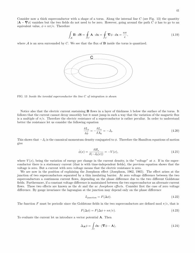
41
Consider now a thick superconductor with a shape of a torus. Along the internal line C (see Fig. 13) the quantity|A −∇φ| vanishes but the two fields do not need to be zero. However, going around the path C φ has to go to anequivalent value, φ + nπ/e. Therefore
∫
AB · dS =
∮
C
A · dx =∮
C
∇φ · dx =nπ
e, (4.19)
where A is an area surrounded by C. We see that the flux of B inside the torus is quantized.
C
FIG. 13 Inside the toroidal superconductor the line C of integration is shown
Notice also that the electric current sustaining B flows in a layer of thickness λ below the surface of the torus. Itfollows that the current cannot decay smoothly but it must jump in such a way that the variation of the magnetic fluxis a multiple of π/e. Therefore the electric resistance of a superconductor is rather peculiar. In order to understandbetter the resistance let us consider the following equation
δLs
δφ= − δLs
δA0= −J0. (4.20)
This shows that −J0 is the canonical momentum density conjugated to φ. Therefore the Hamilton equations of motiongive
φ(x) =δHs
δ(−J0(x))= −V (x), (4.21)
where V (x), being the variation of energy per change in the current density, is the ”voltage” at x. If in the super-conductor there is a stationary current (that is with time-independent fields), the previous equation shows that thevoltage is zero. But a current with zero voltage means that the electric resistance is zero.
We are now in the position of explaining the Josephson effect (Josephson, 1962, 1965). The effect arises at thejunction of two superconductors separated by a thin insulating barrier. At zero voltage difference between the twosuperconductors a continuous current flows, depending on the phase difference due to the two different Goldstonefields. Furthermore, if a constant voltage difference is maintained between the two superconductor an alternate currentflows. These two effects are known as the dc and the ac Josephson effects. Consider first the case of zero voltagedifference. By gauge invariance the lagrangian at the junction may depend only on the phase difference
Ljunction = F (∆φ). (4.22)
The function F must be periodic since the Goldstone fields in the two superconductors are defined mod π/e, that is
F (∆φ) = F (∆φ + nπ/e). (4.23)
To evaluate the current let us introduce a vector potential A. Then
∆Aφ =∫
`
dx · (∇φ−A), (4.24)

42
where the line ` is taken across the junction. Therefore we get
Jk =δLjunction
δAk= nkF ′(∆Aφ), (4.25)
where nk is the normal unit vector at the junction surface. By putting A = 0 we get
J = nF ′(∆φ), (4.26)
showing the dc Josephson effect. To get the second one, consider a constant voltage difference. From
φ = −V, (4.27)
we get
∆φ(t) = |∆V |t + ∆φ(0). (4.28)
Since F has a period π/e it follows that the current oscillates with a frequency
ν =e|∆V |
π. (4.29)
Using this relation one can get a very accurate measure of e/~ (going back to standard units, one has ν = e|∆V |/π~).The current in the dc Josephson effect can be of several milliamperes for conventional superconductors. In the case
of the ac effect for voltages of the order of millivolts, the frequency can rise to hundreds and thousands of gigahertz.When close to the phase transition the description of the theory in terms of the Goldstone boson is not enough.
In fact there is another long wave-length mode associate to the order parameter. This is because the U(1) symmetrygets restored and its minimal description is in terms of a complex field. Therefore one introduces
Φ = ρ e2ieφ. (4.30)
Expanding Ls for small values of Φ we get (with an appropriate normalization for Φ)
Ls ≈∫
d3x[−1
2Φ∗|(∇− 2ieA)|2Φ− 1
2α|Φ|2 − 1
4β|Φ|4
]
=∫
d3x[−2e2ρ2(∇φ− eA)2 − 1
2(∇ρ)2 − 1
2αρ2 − 1
4βρ4
]. (4.31)
In this Section we have defined the penetration depth as the inverse square root of the coefficient of −(∇φ−A)2/2.Therefore
λ =1√
4e2〈ρ2〉 . (4.32)
Using
〈ρ2〉 = −α
β, (4.33)
we get
λ =12e
√−β
α, (4.34)
in agreement with Eq. (1.52) (notice that α and β are not normalized in the same way). Another length is obtainedby studying the behavior of the fluctuations of the field ρ. Defining
ρ = 〈ρ〉+ ρ′, (4.35)
we get
∇2ρ′ = −2αρ′. (4.36)

43
This allows us to introduce the coherence length ξ as
ξ =1√−2α
, (4.37)
in agreement with Eq. (1.59). Using the definitions of λ and ξ we get
α = − 12ξ2
, β = 2e2λ2
ξ2. (4.38)
Therefore the energy density of the superconducting state is lower than the energy density of the normal state by
14
α2
β=
132
1e2λ2ξ2
. (4.39)
The relative size of ξ and λ is very important, since vortex lines can be formed inside the superconductor and theirstability depends on this point. More precisely inside the vortices the normal state is realized, meaning ρ = 0 and aflux-quantized magnetic field. The superconductors are therefore classified according to the following criterium:
• Type I superconductors: ξ > λ. The vortices are not stable since the penetration of the magnetic field is verysmall.
• Type II superconductors: ξ < λ. The vortices are stable and the magnetic field penetrates inside the super-conductor exactly inside the vortices. This may happen since the core of the vortex is much smaller than theregion where the magnetic field goes to zero. In this cases there are two critical magnetic fields, Hc1, wherefor H < Hc1 the state is superconducting, whereas for H > Hc1 vortices are formed. Increasing the magneticfield, more and more vortex lines are formed, up to a value Hc2 where the magnetic field penetrates all thesuperconductor and the transition to the normal state arises.
V. COLOR SUPERCONDUCTIVITY
Ideas about color superconductivity go back to almost 25 years ago (Bailin and Love, 1984; Barrois, 1977; Collinsand Perry, 1975; Frautschi, 1978), but only recently this phenomenon has received a lot of attention (for recent reviewssee ref. (Alford, 2001; Hong, 2001; Hsu, 2000; Nardulli, 2002; Rajagopal and Wilczek, 2001; Schafer, 2003)). Thenaive expectation is that at very high density, due to the asymptotic freedom, quarks would form a Fermi sphere ofalmost free fermions. However, as we know, Bardeen, Cooper and Schrieffer proved that the Fermi surface of freefermions is unstable in presence of an attractive, arbitrary small, interaction. Since in QCD the gluon exchange inthe 3 channel is attractive one expects the formation of a coherent state of Cooper pairs. The phase structure ofQCD at high density depends on the number of flavors and there are two very interesting cases, corresponding totwo massless flavors (2SC) (Alford et al., 1998; Barrois, 1977; Rapp et al., 1998) and to three massless flavors (CFL)(Alford et al., 1999; Schafer and Wilczek, 1999a) respectively. The two cases give rise to very different patterns ofsymmetry breaking. If we denote left- and right-handed quark fields by ψα
iL(R) = ψαia(a) by their Weyl components,
with α = 1, 2, 3, the SU(3)c color index, i = 1, · · · , Nf the flavor index (Nf is the number of massless flavors) anda(a) = 1, 2 the Weyl indices, the structure of the condensate at very high density can be easily understood on thebasis of the following considerations. Consider the matrix element
〈0|ψαiaψβ
jb|0〉. (5.1)
its color, spin and flavor structure is completely fixed by the following considerations:
• The condensate should be antisymmetric in color indices (α, β) in order to have attraction;
• The condensate should be antisymmetric in spin indices (a, b) in order to get a spin zero condensate. Theisotropic structure of the condensate is generally favored since it allows a better use of the Fermi surface (Brownet al., 2000c; Evans et al., 1999a; Schafer, 2000c; Schafer and Wilczek, 1999b);
• given the structure in color and spin, Pauli principles requires antisymmetry in flavor indices.

44
Since the momenta in a Cooper pair are opposite, as the spins of the quarks (the condensate has spin 0), it followsthat the left(right)-handed quarks can pair only with left(right)-handed quarks. In the case of 3 flavors the favoredcondensate is
〈0|ψαiLψβ
jL|0〉 = −〈0|ψαiRψβ
jR|0〉 = ∆3∑
C=1
εαβCεijC . (5.2)
This gives rise to the so-called color–flavor–locked (CFL) phase (Alford et al., 1999; Schafer and Wilczek, 1999a).The reason for the name is that simultaneous transformations in color and in flavor leave the condensate invariant asshown in Fig. 14.
L RC C
<ψψ>LL
<ψψ>RR
rotate colorrotate left rotate right
FIG. 14 Color and flavor indices are represented by black and grey arrows respectively. In the lower part it is shown that wecan leave the left-handed condensate invariant if we perform a flavor rotation followed by a related color rotation. However thisrotates the color index in the right-handed condensate, so in order to have both condensates invariant we have to rotate alsothe right- flavor index. In conclusion we have invariance under the diagonal product of the three SU(3) groups.
More generally the following condensate is formed (Alford et al., 1999; Schafer and Wilczek, 1999a)
〈qαiL(R)Cqβ
jL(R)〉 ∝3∑
C=1
εijCεαβC + κ(δiαδj
β + δiβδj
α). (5.3)
Due to the Fermi statistics, the condensate must be symmetric in color and flavor. As a consequence the two termsappearing in Eq. (5.3) correspond to the (3, 3) and (6,6) channels of SU(3)c ⊗ SU(3)L(R). It turns out that κ issmall (Alford et al., 1999; Schafer, 2000b; Shovkovy and Wijewardhana, 1999) and therefore the condensation occursmainly in the (3, 3) channel. Also in this case the ground state is left invariant by a simultaneous transformation ofSU(3)c and SU(3)L(R). The symmetry breaking pattern is
SU(3)c ⊗ SU(3)L ⊗ SU(3)R ⊗ U(1)B ⊗ U(1)A
↓ (5.4)SU(3)c+L+R ⊗ Z2 ⊗ Z2.
The U(1)A symmetry is broken at the quantum level by the anomaly, but it gets restored at very high density sincethe instanton contribution is suppressed (Rapp et al., 2000; Schafer, 2000b; Son and Stephanov, 2000a,b). The Z2

45
symmetries arise since the condensate is left invariant by a change of sign of the left- and/or right-handed fields. Theelectric charge is broken but a linear combination with the broken color generator T8 annihilates the ground state.On the contrary the baryon number is broken. Therefore there are 8 + 2 broken global symmetries giving rise to 10Goldstone bosons. The one associated to U(1)A gets massless only at very high density. The color group is completelybroken and all the gauge particles acquire mass. Also all the fermions are gapped. We will show in the following howto construct an effective lagrangian describing the Goldstone bosons, and how to compute their couplings in the highdensity limit where the QCD coupling gets weaker.
The previous one is the typical situation when the chemical potential is much bigger than the quark masses mu,md and ms (here the masses to be considered are in principle density depending). However we may ask what happensdecreasing the chemical potential. At intermediate densities we have no more the support of asymptotic freedom, butall the model calculations show that one still has a sizeable color condensation. In particular if the chemical potentialµ is much less than the strange quark mass one expects that the strange quark decouples, and the correspondingcondensate should be
〈0|ψαiLψβ
jL|0〉 = ∆εαβ3εij . (5.5)
In fact, due to the antisymmetry in color the condensate must necessarily choose a direction in color space. Noticethat now the symmetry breaking pattern is completely different from the three-flavor case:
SU(3)c ⊗ SU(2)L ⊗ SU(2)R ⊗ U(1)B → SU(2)c ⊗ SU(2)L ⊗ SU(2)R ⊗ U(1)⊗ Z2.
The condensate breaks the color group SU(3)c down to the subgroup SU(2)c but it does not break any flavor symmetry.Although the baryon number, B, is broken, there is a combination of B and of the broken color generator, T8, whichis unbroken in the 2SC phase. Therefore no massless Goldstone bosons are present in this phase. On the other hand,five gluon fields acquire mass whereas three are left massless. We notice also that for the electric charge the situationis very similar to the one for the baryon number. Again a linear combination of the broken electric charge and of thebroken generator T8 is unbroken in the 2SC phase. The condensate (5.5) gives rise to a gap, ∆, for quarks of color 1and 2, whereas the two quarks of color 3 remain un-gapped (massless). The resulting effective low-energy theory hasbeen described in (Casalbuoni et al., 2000, 2001a; Rischke et al., 2001).
A final problem we will discuss has to do with the fact that when quarks (in particular the strange quark) aremassive, their chemical potentials cannot be all equal. This situation has been modelled out in (Alford et al., 2001).If the Fermi surfaces of different flavors are too far apart, BCS pairing does not occur. However it might be favorable fordifferent quarks to pair each of one lying at its own Fermi surface and originating a pair of non-zero total momentum.This is the LOFF state first studied by the authors of ref. (Fulde and Ferrell, 1964; Larkin and Ovchinnikov, 1964) inthe context of electron superconductivity in the presence of magnetic impurities. Since the Cooper pair has non-zeromomentum the condensate breaks space symmetries and we will show that in the low-energy spectrum a masslessparticle, a phonon, the Goldstone boson of the broken translational symmetry, is present. We will construct theeffective lagrangian also for this case (for a general review of the LOFF phase see (Bowers, 2003; Casalbuoni andNardulli, 2003).
Of course it would be very nice if we could test all these ideas on the lattice. However the usual sampling method,which is based on a positive definite measure, does not work in presence of a chemical potential since the fermionicdeterminant turns out to be complex in euclidean space. The argument is rather simple. We define euclidean variablesthrough the following substitutions
x0 → −ix4E , xi → xi
E , (5.6)γ0 → γ4
E , γi → −iγiE . (5.7)
Then the Dirac operator, in presence of a chemical potential, becomes4
D(µ) = γµEDµ
E + µγ4E , (5.8)
where DµE = ∂µ
E + iAµE is the euclidean covariant derivative. In absence of a chemical potential the operator has the
following properties
D(0)† = −D(0), γ5D(0)γ5 = −D(0). (5.9)
4 We neglect the mass term, since it correspond to an operator multiple of the identity, and all the following considerations can be triviallyextended.

46
Therefore the eigenvalues of D(0) are pure imaginary. Also if |λ〉 is an eigenvector of D(0), the same is for γ5|λ〉 butwith eigenvalue −λ. This follows from
γ5D(0)|λ〉 = λγ5|λ〉 = −D(0)γ5|λ〉. (5.10)
Therefore
det[D(0)] =∏
λ
(λ)(−λ) > 0. (5.11)
For µ 6= 0 this argument does not hold and the determinant is complex. Notice that this argument depends on thekind of chemical potential one has to do. For instance in the case of two degenerate flavored quarks, u and d, if weconsider the isospin chemical potential, which is coupled to the conserved charge τ3 in flavor space, we may still provethe positivity by using, for instance, τ1γ5 instead of γ5. Therefore these cases can be treated on the lattice.
A. Hierarchies of effective lagrangians
QCD at high density is conveniently studied through a hierarchy of effective field theories. The starting point is thefundamental QCD lagrangian. The way of obtaining a low energy effective lagrangian is to integrate out high-energydegrees of freedom. As we have seen Polchinski (Polchinski, 1993) has shown that the physics is particularly simplefor energies close to the Fermi energy. He has shown that all the interactions are irrelevant except for a four-fermiinteraction coupling pair of fermions with opposite momenta. This is nothing but the interaction giving rise to theBCS condensation. This physics can be described using the High Density Effective Theory (HDET) (Beane et al.,2000; Casalbuoni et al., 2001c,d; Hong, 2000a,b).
pF
pF
+ ∆
pF
+ δ
δ
∆
∆ << δ << pF
LQCD
L HDET
LGolds
FIG. 15 The hierarchy of effective lagrangians entering in the discussion of high density QCD.
In this theory the condensation effects are taken into account through the introduction of a Majorana mass term.The degrees of freedom are quasi-particles (dressed fermions), holes and gauge fields. This description is supposedto hold up to a cutoff pF + δ, with δ smaller than the Fermi momentum but bigger than the gap ∆, ∆ ¿ δ ¿ pF .Going at momenta much smaller than the gap energy ∆ all the gapped particles decouple and one is left with thelow energy modes as Goldstone bosons, ungapped fermions and holes and massless gauged fields according to thebreaking scheme. The corresponding effective theory in the Goldstone sector can be easily formulated using standardtechniques. In the case of CFL and 2SC such effective lagrangians have been given in refs. (Casalbuoni and Gatto,1999) and (Casalbuoni et al., 2000; Rischke et al., 2001). The parameters of the effective lagrangian can be evaluatedat each step of the hierarchy by matching the Greens functions with the ones evaluated at the upper level.

47
B. The High Density Effective Theory (HDET)
We will present here the High Density Effective Theory (Beane et al., 2000; Casalbuoni et al., 2001c,d; Hong,2000a,b) in the context of QCD with Nf massless flavors. As already discussed we will integrate out all the fermionicdegrees of freedom corresponding to momenta greater than pF + δ with δ a cutoff such that ∆ ¿ δ ¿ pF . The QCDlagrangian at finite density is given by
LQCD = ψiD/ ψ − 14F a
µνF aµν + µψγ0ψ, a = 1, · · · , 8, (5.12)
Dµ = ∂µ + igsAaµT a, D/ = γµDµ, (5.13)
where T a = λa/2, with λa the Gell-Mann matrices. At asymptotic values of µ À ΛQCD quarks can be considered asalmost free particles due to the asymptotic freedom. The corresponding Dirac equation in momentum space is
(p/ + µγ0)ψ(p) = 0, (5.14)
or
(p0 + µ)ψ(p) = α · pψ(p), (5.15)
where α = γ0γ. From this we get immediately the dispersion relation
(p0 + µ)2 = |p|2, (5.16)
or
p0 = E± = −µ± |p|. (5.17)
For the following it is convenient to write the Dirac equation in terms of the following projectors
P± =1±α · vF
2, (5.18)
where
v ≡ vF =∂E(p)
∂p=
∂|p|∂p
= p. (5.19)
Decomposing p = µvF + ` we get
Hψ+ = α · ` ψ+, Hψ− = (−2µ + α · `) ψ−. (5.20)
Therefore only the states ψ+ with energies close to the Fermi surface, |p| ≈ µ can be easily excited (E+ ≈ 0). Onthe contrary, the states ψ− have E− ≈ −2µ. They are well inside the Fermi sphere and decouple for high values ofµ. In the limit µ → ∞ the only physical degrees of freedom are ψ+ and the gluons. After this quantum mechanicalintroduction, let us consider the field theoretical version of the previous argument. The main idea of the effectivetheory is the observation that the quarks participating in the dynamics have large (∼ µ) momenta. Therefore onecan introduce velocity dependent fields by extracting the large part µv of this momentum. We start with the Fourierdecomposition of the quark field ψ(x):
ψ(x) =∫
d4p
(2π)4e−i p·xψ(p), (5.21)
and then we introduce the Fermi velocity as
pµ = µvµ + `µ , (5.22)
where
vµ = (0,v), (5.23)

48
with |v| = 1. The four-vector
`µ = (`0, ~), (5.24)
is called the residual momentum. We define also
` = v`‖ + `⊥, (5.25)
with
`⊥ = `− (` · v)v. (5.26)
Since we can always choose the velocity v parallel to p, we have `⊥ = 0. We will now separate in Eq. (5.21) the lightand heavy fermion degrees of freedom. These are defined by the following restrictions in momentum space:
light d.o.f. µ− δ ≤ |p| ≤ µ + δ,
heavy d.o.f. |p| ≤ µ− δ, |p| ≥ µ + δ, (5.27)
or, in terms of the residual momentum
light d.o.f. − δ ≤ `‖ ≤ +δ,
heavy d.o.f. `‖ ≤ −δ, `‖ ≥ +δ. (5.28)
Here δ is the cutoff that we choose for defining the effective theory around the Fermi sphere. We will assume thatδ À ∆, with ∆ the gap. We will assume also that the shell around the Fermi sphere is a narrow one and thereforeδ ¿ µ. Let us start our discussion with the light fields. We will discuss how to integrate out the heavy d.o.f later on.In this case we can write the integration in momentum space in the form
∫d4p
(2π)4=
µ2
(2π)4
∫dΩ
∫ +δ
−δ
d`‖
∫ +∞
−∞d`0 =
∫dv4π
µ2
π
∫d2`
(2π)2, (5.29)
where we have taken into account that we are interested in the degrees of freedom in a shell of amplitude 2δ aroundthe Fermi sphere, and that in the shell we can assume a constant radius µ. We have also substituted the angularintegration with the integration over the Fermi velocity taking into account that it is a unit vector. That is
∫dv ≡
∫d3vδ(|v| − 1) =
∫|v|2 d|v| dΩ δ(|v| − 1) =
∫dΩ. (5.30)
In this way the original 4-dimensional integration in momentum has been factorized in the product of two 2-dimensionalintegrations. In particular
∫
|p|∈shell
d3p(2π)3
=∫
dv4π
µ2
π
∫d`‖. (5.31)
The Fourier decomposition (5.21) for the light d.o.f. takes the form
ψ(x) =∫
dv4π
e−iµv·xψv(x) , (5.32)
where
ψv(x) =µ2
π
∫d2`
(2π)2e−i`·x ψv(`), (5.33)
with ψv(`) ≡ ψ(p). Notice that the fields ψv(x) are velocity-dependent and they include only the degrees of freedomcorresponding to the shell around the Fermi sphere. Projecting with the operators P± we get
ψ(x) =∫
dv4π
e−iµv·x [ψ+(x) + ψ−(x)] , (5.34)
where
ψ±(x) = P±ψv(x) = P±µ2
π
∫d2`
(2π)2e−i`·xψv(`). (5.35)

49
Let us now define
V µ = (1, v) , V µ = (1, −v) ,
γµ‖ = (γ0, (v · γ)v) , γµ
⊥ = γµ − γµ‖ . (5.36)
We can then prove the following relations
ψ+γµψ+ = V µψ+γ0ψ+ ,
ψ−γµψ− = V µψ−γ0ψ− ,ψ+γµψ− = ψ+γµ
⊥ψ− ,ψ−γµψ+ = ψ−γµ
⊥ψ+. (5.37)
Now we want to evaluate the effective action in terms of the velocity-dependent fields defined in Eqs. (5.32) and(5.33). Substituting the expression (5.33) in terms of the type
∫d4xψ†ψ we find
∫d4xψ†ψ =
(µ2
π
)2 ∫d~vF
4π
d~v′F4π
d2`
(2π)2d2`′
(2π)2(2π)4δ4(`′ − ` + µv′ − µv)ψ†v′(`
′)ψv(`). (5.38)
For large values of µ the integral is different from zero only if v = v′ and the δ-function factorizes in the product oftwo δ-functions one for the velocity and one for the residual momenta. Both these δ-functions are two-dimensional.Therefore we obtain
∫d4x ψ†ψ =
µ2
π
∫dv4π
d2`
(2π)2ψ†v(`)ψv(`). (5.39)
Analogously one could start from (5.32) finding∫
d4xψ†ψ =∫
d4x
∫dv4π
ψ†v(x)ψv(x). (5.40)
In the following we will need also the expression∫
d4xψT Cψ. We find∫
d4xψT Cψ =∫
d4x
∫dv4π
ψTv (x)Cψ−v(x) =
µ2
π
∫dv4π
d2`
(2π)2ψT
v (`)Cψ−v(−`). (5.41)
These expressions show that there is a superselection rule for the Fermi velocity.Now we are in the position to evaluate the effective lagrangian for the fields ψ+ which should be the relevant degrees
of freedom in the high density limit. Since we have
i∂µe−iµv·x = µvµe−iµv·x, (5.42)
we get∫
d4x ψ(iD/ + µγ0
)ψ =
∫d4x
∫dv4π
(ψ+ + ψ−)[µ(v/ + γ0) + iD/
](ψ+ + ψ−). (5.43)
Expanding and using Eqs. (5.37) we find∫
d4x ψ(iD/ + µγ0
)ψ =∫
d4x(ψ†+iV ·Dψ+ + ψ†−iV ·Dψ− + 2µψ†−ψ− + ψ+iD/ ⊥ψ− + ψ−iD/ ⊥ψ+
). (5.44)
The lagrangian is given by
LD =∫
dv4π
[ψ†+iV ·Dψ+ + ψ†−(2µ + iV ·D)ψ− + (ψ+iD/ ⊥ψ− + h.c.)
]. (5.45)
From which we get the equations of motion
iV ·Dψ+ + iγ0D/ ⊥ψ− = 0,

50
(2µ + iV ·D)ψ− + iγ0D/ ⊥ψ+ = 0. (5.46)
At the leading order in 1/µ
ψ− = 0, iV ·Dψ+ = 0, (5.47)
proving the decoupling of ψ−. At this order the effective lagrangian is simply
LD =∫
dv4π
ψ†+iV ·Dψ+. (5.48)
Therefore the free propagator, 〈T (ψ+ψ†+)〉, is given by
1V · ` . (5.49)
This can be seen directly starting from the Dirac propagator
1p0γ0 − ~p · ~γ + µγ0
=(p0 + µ)γ0 − ~p · ~γ(p0 + µ)2 − |~p |2 . (5.50)
By putting p = µv + ` and expanding at the leading order in 1/µ we find
1p/ + µγ0
≈ V/
21
V · ` , (5.51)
where V · ` = `0 − ` · v. Therefore the propagator depends (at the leading order) only on the energy `0 and on themomentum perpendicular to the Fermi surface `‖ = ` · v. Notice also that
V/
2=
12γ0(1−α · v) = P+γ0. (5.52)
Recalling that the Dirac propagator is the ψψ T -product, we see that the propagator 〈T (ψ+ψ†+)〉 at this order is just1/V · `.
1. Integrating out the heavy degrees of freedom
All the steps leading to Eq. (5.45) can be formally performed both for light and heavy degrees of freedom. However,in order to integrate out the heavy fields we need to write the effective lagrangian at all orders in µ in the followingnon-local form :
L = −14F a
µνF aµν + LD , (5.53)
where
LD =∫
dv4π
[ψ†+iV ·Dψ+ − ψ†+
12µ + iV ·DD/
2⊥ψ+
]. (5.54)
Using the identity
ψ†+γµ⊥γν
⊥ψ+ = ψ†+Pµνψ+, (5.55)
where
Pµν = gµν − 12
[V µV ν + V ν V µ
], (5.56)

51
we can write (5.54) as:
LD =∫
dv4π
[ψ†+iV ·Dψ+ − Pµνψ†+
12µ + iV ·DDµDνψ+
]. (5.57)
Notice that the Eq. (5.33) does not hold in this case. We need now to decompose the fields in light and heavycontributions
ψ+ = ψl+ + ψh
+. (5.58)
Substituting inside Eq. (5.57) we get
LD = LlD + Llh
D + LhD, (5.59)
where LlD is nothing but (5.48) at the leading order in µ:
LlD =
∫dv4π
ψl†+iV ·Dψl
+, (5.60)
whereas
LlhD =
∫dv4π
(ψl†
+iV ·Dψh+ − Pµνψl†
+
12µ + iV ·DDµDνψh
+ + (l ↔ h))
(5.61)
and
LhD =
∫dv4π
(ψh†
+ iV ·Dψh+ − Pµνψh†
+
12µ + iV ·DDµDνψh
+
). (5.62)
When we integrate out the heavy fields, the terms arising from LlhD produce diagrams with two light fermions external
lines and a bunch of external gluons with a heavy propagator (see, for instance Fig. 16). Due to the momentum
FIG. 16 Some of the operators arising from integrating out the heavy degrees of freedom in LlhD . The wavy lines represent the
gluons, the thin lines the light fermionic d.o.f. and the thick lines the heavy ones
conservation they can contribute only if some of the gluon momenta are harder than δ. However the hard gluons aresuppressed by asymptotic freedom. Notice that these terms may also give rise to pure gluon terms by closing the lightline in the loop, see Fig. 17.
On the other hand the second term in LhD can contribute to an operator containing only soft gluon external lines and
a loop of heavy fermions at zero momentum (see for instance in Fig. 18 the contribution to the two gluon operator).Notice that the heavy fermion propagator comes from the first term in Lh
D and it coincides with the propagatorevaluated for the free Fermi gas in Section II.A. This is so also in case of condensation since we are assuming δ À ∆.Furthermore, from Eq. (2.38) we know that the propagator at zero momentum is nothing but the density of states

52
FIG. 17 A contribution to hard gluon terms obtained by closing the light fermion lines in the diagrams of Fig. 16
FIG. 18 The two gluon operator arising from integrating out the heavy degrees of freedom in LhD. The wavy lines represent the
gluons, the thin lines the light fermionic d.o.f. and the thick lines the heavy oneslight
inside the Fermi surface. Therefore we expect an order µ3 contribution5. At the leading order in µ this gives a termof the type µ2A2, where A is the gluon field. We will evaluate this contribution later in Section VIII.A. Since thisis a mass term for the gluons and, as we shall see, gives a contribution only to the spatial gluons, it will be referredto as bare Meissner mass. The result of this discussion is that the effective lagrangian for the light fields is simplygiven by Ll
D, plus terms containing powers of soft gluon fields.
2. The HDET in the condensed phase
Let us now see what happens in the case of condensation after having integrated out the heavy fields. We will omitfrom now on the superscript identifying the light fields since these are the only fields we will deal with from now on.We will describe color and flavor with a collective index A = 1, · · · , N (N = NcNf ). The general structure of thecondensate, both for left- and right- handed fields is (we will neglect from now on the Weyl indices since we assumethe difermions in the spin 0 state)
〈ψACψB〉 ≈ ∆AB , (5.63)
with ∆AB a complex symmetric matrix.We will now consider a four-fermi interaction of the BCS type
LI = −G
4εabεabVABCDψA
a ψBb ψC†
a ψD†b
. (5.64)
We require LI to be hermitian, therefore
VABCD = V ∗CDAB (5.65)
and furthermore
VABCD = VBACD = VABDC . (5.66)
As we have done in Section III.D we write
LI = Lcond + Lint, (5.67)
5 To be precise we should take out the volume of the portion of the shell inside the Fermi surface that goes in the light fields definition,but since we are taking the limit of large µ this is negligible.
53
with
Lcond =G
4VABCDΓCD∗ψAT CψB − G
4VABCDΓABψC†CψD∗ (5.68)
and
Lint = −G
4VABCD
(ψAT CψB − ΓAB
) (ψC†CψD∗ + ΓCD∗) . (5.69)
We now define
∆AB =G
2VCDABΓCD, ∆∗
AB =G
2V ∗
CDABΓCD∗ =G
2VABCDΓCD∗. (5.70)
Clearly ∆AB is a symmetric matrix. We will assume also that it can be diagonalized, meaning that
[∆,∆†] = 0, (5.71)
where ∆AB = ∆AB . Therefore (C is the charge conjugation matrix, C = iσ2)
Lcond =12∆∗
ABψAT CψB − 12∆ABψA†CψB∗. (5.72)
For the following it is convenient to introduce the following notation for the positive energy fields:
ψ±(x) = ψ+(±v, x). (5.73)
One should be careful in not identifying ψ− with the negative energy solution with velocity v. The condensationis taken into account by adding Lcond to the effective lagrangian of the previous Section (here we consider only theleading term), see Sections III.C and III.D. Therefore we will assume the following Lagrangian
LD =∫
dv4π
∑
A,B
[ψA†
+ (iV ·D)ABψB+ +
12ψA−CψB
+∆∗AB −
12ψA†
+ CψB∗− ∆AB
]. (5.74)
Using the symmetry v → −v of the velocity integration we may write the previous expression in the form
LD =∫
dv4π
∑
A,B
12
[ψA†
+ (iV ·D)ABψB+ + ψA†
− (iV ·D)ABψB− + ψA
−CψB+∆∗
AB − ψA†+ CψB∗
− ∆AB
]. (5.75)
We then introduce the Nambu-Gor’kov basis
χA =1√2
(ψA
+
CψA∗−
)(5.76)
in terms of which
LD =∫
dv4π
χA†[
iV ·DAB −∆AB
−∆∗AB iV ·D∗
AB
]χB . (5.77)
The lagrangian we have derived here coincides with the one that we obtained in Section III.D, that is the lagrangiangiving rise to the Nambu-Gor’kov equations.
The inverse free propagator in operator notations is (notice that since ∆ is symmetric we have ∆∗ = ∆†)
S−1(`) =(
V · ` −∆−∆† V · `
). (5.78)
From which
S(`) =1
(V · `)(V · `)−∆∆†
(V · ` ∆∆† V · `
). (5.79)
Let us now consider the relation
∆∗AB = −G
2VABCD〈ψC†CψD∗〉. (5.80)

54
This Equation is the analogous of Eq. (3.112) in configuration space. Repeating the same steps leading to Eq. (3.130)we find
∆∗AB = i 2× G
2VABCD
∫dv4π
µ2
π
∫d2`
(2π)2∆∗
CE
1DED
, (5.81)
where we have made use of Eq. (5.31) and
1DAB
=(
1(V · `)(V · `)−∆∆†
)
AB
. (5.82)
Notice that the factor 2 arises from the sum over the Weyl indices. The final result is
∆∗AB = iGVABCD
∫dv4π
µ2
π
∫d2`
(2π)2∆∗
CE
1DED
, (5.83)
in agreement with the result we found from the Nambu-Gor’kov equations by identifying E with `0 and d3p with theintegration over the velocity and `‖. The same result can be found via the functional approach, see Appendix A.
Let us apply this formalism to the case of an effective four-fermi interaction due to one gluon exchange
LI =316
Gψγµλaψψγµλaψ, (5.84)
where λa are the Gell-Mann matrices. Using the following identities
8∑a=1
(λa)αβ(λa)δγ =23
(3δαγδβδ − δαβδγδ) (5.85)
and
(σµ)ab(σµ)dc = 2εacεbd (5.86)
where
σµ = (1, σ), σµ = (1,−σ), (5.87)
with σ the Pauli matrices, we find
LI = −G
4V(αi)(βj)(γk)(δ`)ψ
αi ψβ
j ψγ†k ψδ†
` (5.88)
with
V(αi)(βj)(γk)(δ`) = −(3δαδδβγ − δαγδβδ)δikδj`. (5.89)
Let us now consider the simple case of the 2SC phase. Then, as we have seen,
∆(αi)(βj) = εαβ3εij∆. (5.90)
We get at once
∆ = 4iG
∫dv4π
µ2
π
∫d2`
(2π)2∆
`20 − `2‖ −∆2, (5.91)
with `‖ = v · `. Performing the integration over `0 we obtain
∆ =G
2ρ
∫ δ
0
dξ∆√
ξ2 + ∆2. (5.92)
Here we have defined the density of states as
ρ =4µ2
π2, (5.93)

55
which is the appropriate one for this case. In fact remember that in the BCS case the density is defined as p2F /vF π2.
In the actual case pF = EF = µ and vF = 1. The factor 4 arises since there are 4 fermions, ψαi with α = 1, 2, which
are pairing.It is worth to note that an alternative approach is to work directly with the Schwinger-Dyson equation (Rajagopal
and Wilczek, 2001). In that case there is no necessity to Fierz transform the interaction term. The reason we have notadopted this scheme, although technically more simple, is just to illustrate more the similarities with the condensedmatter treatment.
In order to make an evaluation of the gap one can fix the coupling by the requirement that this theory reproducesthe chiral phenomenology in the limit of zero density and temperature. It is not difficult to show that the chiral gapequation is given by
1 = 8G
∫ Λ
0
d3p(2π)3
1√p2 + M2
. (5.94)
Here Λ is the Nambu Jona-Lasinio cutoff and M is the constituent mass. Correspondingly one chooses δ = Λ−µ in thegap equation at finite density. By choosing typical values of Λ = 800 MeV , M = 400 MeV and µ = 400÷ 500 MeVone finds respectively ∆ = 39÷ 88 MeV 6. Similar values are also found in the CFL case.
C. The gap equation in QCD
Having discussed the gap equation in the context of a four-fermi interaction we will now discuss the real QCD case.However this calculation has real meaning only at extremely high densities much larger than 108 MeV , see (Rajagopaland Shuster, 2000). Therefore we will give only a brief sketch of the main results. We will work in the simpler caseof the 2SC phase.
∆
=
∆
FIG. 19 The gap equation in QCD at finite density. The light grey circle denotes the gluon self-energy insertion. The dark greyones a gap insertions. At the leading order there is no need of vertex corrections
As shown in Appendix A the gap equation can be obtained simply by writing down the Schwinger-Dyson equation,as shown in Fig. 19. The diagram has been evaluated in (Brown et al., 2000b; Hong et al., 2000b; Pisarski andRischke, 2000a; Schafer and Wilczek, 1999d; Son, 1999). The result in euclidean space is
∆(p0) =g2
12π2
∫dq0
∫d cos θ
( 32 − 1
2 cos θ
1− cos θ + G/(2µ2)
+12 + 1
2 cos θ
1− cos θ + F/(2µ2)
)∆(q0)√
q20 + ∆(q0)2
. (5.95)
Here, ∆(p0) is the energy dependent gap, g is the QCD coupling constant and G and F are the self energies ofmagnetic and electric gluons. The terms in the curly brackets arise from the magnetic and electric components of thegluon propagator. The numerators are the on-shell matrix elements Mii,00 = [uh(p1)γi,0uh(p3)][uh(p2)γi,0uh(p4)] for
6 For a different way of choosing the cutoff in NJL models, see (Casalbuoni et al., 2003)

56
the scattering of back-to-back fermions on the Fermi surface. The scattering angle is cos θ = p1 · p3. In the case of aspin zero order parameter, the helicity h of all fermions is the same (see (Schafer and Wilczek, 1999d)).
The important difference between Eq. (5.95) and the case of a contact four-fermi interaction is due to the factthat the self-energy of the magnetic gluons vanishes at zero energy. Therefore the gap equation contains a collinearcos θ ∼ 1 divergence. One makes use of the hard-loop approximation (Le Bellac, 1996) and for q0 ¿ |q| → 0 and toleading order in perturbation theory we have
F = m2D, G =
π
4m2
D
q0
|~q| , (5.96)
with
m2D = Nf
g2µ2
2π2. (5.97)
In the electric part, m2D is the Debye screening mass. In the magnetic part, there is no screening of static modes, but
non-static modes are dynamically screened due to Landau damping. For small energies dynamic screening of magneticmodes is much weaker than Debye screening of electric modes. As a consequence, perturbative color superconductivityis dominated by magnetic gluon exchanges. We are now able to perform the angular integral in Eq. (5.95) finding
∆(p0) =g2
18π2
∫dq0 log
(bµ
|p0 − q0|)
∆(q0)√q20 + ∆(q0)2
, (5.98)
with
b = 256π4(2/Nf )5/2g−5. (5.99)
This equation has been derived for the first time in QCD in Ref. (Son, 1999). In ordinary superconductivity it wasrealized by (Eliashberg, 1960) that the effects of retardation of phonons (taking the place of the gluons) are importantand that they produce the extra logarithmic term in the gap equation. The integral equation we have obtained canbe converted to a differential equation (Son, 1999) and in the weak coupling limit an approximate solution is (Brownet al., 2000a,b,c; Pisarski and Rischke, 1999, 2000a,b; Schafer and Wilczek, 1999d; Son, 1999)
∆(p0) ≈ ∆0 sin(
g
3√
2πlog
(b
p0
)), (5.100)
with
∆0 = 2bµ exp(− 3π2
√2g
). (5.101)
This result shows why it is important to keep track of the energy dependence of ∆. In particular neglecting the energydependence would give a wrong coefficient in the exponent appearing in ∆0. Also we see that the collinear divergenceleads to a gap equation with a double-log behavior. Qualitatively
1 ∼ g2
18π2
[log
( µ
∆
)]2
, (5.102)
from which we conclude that ∆ ∼ exp(−c/g). The prefactor in the expression for ∆0 is not of easy evaluation. Bywriting
∆0 ' 512π4(2/Nf )5/2b′0µg−5 exp(− 3π2
√2g
). (5.103)
we have b′0 = 1 in the previous case, whereas with different approximations in (Brown et al., 2000c; Wang and Rischke,2002) it has been found
b′0 = exp(−4 + π2
8
). (5.104)
Numerically one finds at µ = 1010 MeV , g = .67 and b′0 = 2/5, ∆0 ≈ 40 MeV . Extrapolating at µ = 400 MeV ,g = 3.43, one finds ∆0 ≈ 90 MeV . It turns out that ∆0 decreases from 90 MeV to about 10 MeV for µ increasingfrom 400 MeV to 106 MeV . Continuing to increase µ ∆ increases as it should be according to its asymptotic value.In fact we see that for increasing µ, ∆ increases although ∆/µ → 0. In particular we notice that neither the four-fermi interaction approach and the present one from first principles can be trusted at phenomenologically interestingchemical potentials of the order 400÷ 500 MeV . Still it is of some interest to observe that both methods lead to gapsof the same order of magnitude.

57
D. The symmetries of the superconductive phases
1. The CFL phase
As we have already discussed we expect that at very high density the condensate 〈ψαiLCψβ
jL〉 is antisymmetric incolor and in flavor. Also, if we require parity invariance we have
〈ψαiLψβ
jL〉 = −〈ψαiRψβ
jR〉. (5.105)
In fact in Dirac notation we notice that
〈ψT Cγ5ψ〉 (5.106)
is parity invariant (ψ → ηP γ0ψ) and its L and R components are precisely 〈ψLψL〉 and 〈ψRψR〉. The requiredantisymmetry implies
〈ψαiLψβ
jL〉 = εαβγεijkAkγ , (5.107)
with A a 3×3 matrix. In (Evans et al., 2000) it has been shown that A can be diagonalized by using an SU(3)c⊗SU(3)L
global rotation
A → gSU(3)cAgSU(3)L
= AD, (5.108)
with
AD =
(a 0 00 b 00 0 c
). (5.109)
Studying the gap equation (this calculation has been done in full QCD) it can be seen that three cases are possible
(1, 1, 1) : AD =
( 1 0 00 1 00 0 1
)
(1, 1, 0) : AD =
( 1 0 00 1 00 0 0
)
(1, 0, 0) : AD =
( 1 0 00 0 00 0 0
). (5.110)
The corresponding gaps satisfy
∆(1,1,1) < ∆(1,1,0) < ∆(1,0,0), (5.111)
but for the free energies the result is
F(1,1,1) < F(1,1,0) < F(1,0,0). (5.112)
The reason is that although the gaps for the less symmetric solution is bigger, there are more fermions paired in themore symmetric configurations.
The analysis of the gap equation shows that there is also a component from the color channel 6. In fact, under thegroup SU(3)c ⊗ SU(3)L ⊗ SU(3)R we have
ψαiL(R) ∈ (3c,3L(R)). (5.113)
Therefore[(3c,3L(R))⊗ (3c,3L(R))
]S
= (3∗c ,3∗L(R))⊕ (6c,6L(R)). (5.114)
Here the index S means that we have to take the symmetric combination of the tensor product since 〈ψTLCψL〉 is
already antisymmetric in spin. From the previous argument and in the absence of the (6c,6L(R)) component we have
〈ψαiLψβ
jL〉 = ∆εαβIεijI . (5.115)

58
The presence of the (6c,6L(R)) implies
〈ψαiLψβ
jL〉 = ∆εαβIεijI + ∆6(δαi δβ
j + δβi δα
j ), (5.116)
or
〈ψαiLψβ
jL〉 = ∆(δαi δβ
j − δβi δα
j ) + ∆6(δαi δβ
j + δβi δα
j ) = (∆ + ∆6)δαi δβ
j + (∆6 −∆)δβi δα
j . (5.117)
Notice that the (6c,6L(R)) term does not break any further symmetry other than the ones already broken by the(3∗c ,3
∗L(R)). Numerically ∆6 turns out to be quite small. The analysis has been done in (Alford et al., 1999) using
the parameters ∆8 and ∆1, defined as
∆ + ∆6 =13
(∆8 +
18∆1
), ∆−∆6 = −1
8∆1. (5.118)
Therefore
∆ =13
(∆8 −∆1) , ∆6 =16
(∆8 +
12∆1
). (5.119)
The absence of the sextet is equivalent to require ∆1 = −2∆8. The result found in (Alford et al., 1999), for the choiceof parameters, Λ = 800 MeV , M = 400 MeV and µ = 400 MeV is
∆8 = 80 MeV, ∆1 = −176 MeV, (5.120)
implying
∆ = 85.3 MeV, ∆6 = −1.3 MeV. (5.121)
As already discussed the original symmetry of the theory is
GQCD = SU(3)c ⊗ SU(3)L ⊗ SU(3)R ⊗ U(1)B . (5.122)
The first factor is local whereas the other three are global since, for the moment, we are neglecting the em interactionwhich makes local a U(1) subgroup of SU(3)L ⊗ SU(3)R. The condensates lock together the transformations ofSU(3)c, SU(3)L and SU(3)R, therefore the symmetry of the CFL phase is
GCFL = SU(3)c+L+R ⊗ Z2. (5.123)
In fact, also the U(1)B group is broken leaving a Z2 symmetry corresponding to the multiplication of the quark fieldsby -1. Also, locking SU(3)L and SU(3)R to SU(3)c makes SU(3)L and SU(3)R lock together producing the breakingof the chiral symmetry. The breaking of GQCD to GCFL gives rise to
3× 8 + 1− 8 = 8 + 8 + 1 (5.124)
Nambu-Goldstone (NB) bosons. However 8 of the NG bosons disappear from the physical spectrum through theHiggs mechanism, giving masses to the 8 gluons, whereas 8+1 massless NG bosons are left in the physical spectrum.Of course, these NG bosons take mass due to the explicit breaking of the symmetry produced by the quark masses.Since all the local symmetries are broken (but see later as far the electromagnetism is concerned) all the gauge bosonsacquire a mass.
Although the baryon number is broken no dramatic event takes place. The point is that we are dealing with afinite sample of superconductive matter. In fact, applying the Gauss’ law to a surface surrounding the sample we findthat changes of the baryon number inside the superconductor must be accompanied by compensating fluxes. In otherwords, inside the sample there might be large fluctuations and transport of baryonic number. Things are not differentfrom what happens in ordinary superconductors where the quantum number, number of electrons (or lepton number),is not conserved. The connection between the violation of quantum numbers and phenomena of supertransport assuperfluidity and superconductivity are very strictly related.
The condensate 〈ψαiLψβ
jL〉 is not gauge invariant and we may wonder if it is possible to define gauge invariant orderparameters. To this end let us introduce the matrices
Xkγ = 〈ψα
iLψβjL〉∗εαβγεijk, Y k
γ = 〈ψαiRψβ
jR〉∗εαβγεijk. (5.125)

59
The conjugation has been introduced for convenience reasons (see in the following). The matrix
(Y †X)ij =
∑α
(Y jα )∗Xi
α (5.126)
is gauge invariant, since color indices are saturated and breaks SU(3)L ⊗ SU(3)R to SU(3)L+R. Analogously the6-fermion operators
det(X), det(Y ) (5.127)
are gauge invariant flavor singlet and break U(1)B .So far we have neglected U(1)A. This group is broken by the anomaly. However, the anomaly is induced by a
6-fermion operator (the ’t Hooft determinant) which becomes irrelevant at the Fermi surface. On the other hand thisoperator is qualitatively important since it is the main cause of the breaking of U(1)A. If there was no such operatorwe would have a further NG boson associated to the spontaneous breaking of U(1)A produced by the di-fermioncondensate. Since the instanton contribution is parametrically small at high density, we expect the NG boson to bevery light. Notice that the U(1)A approximate symmetry is broken by the condensate to a discrete group Z2.
The spectrum of the CFL phase
Let us spend some word about the spectrum of QCD in the CFL phase. We start with the fermions. Since all thefermions are paired they are all gapped. To understand better this point let us notice that under the symmetry groupof the CFL phase SU(3)c+L+R quarks transform as 1⊕ 8. Therefore it is useful to introduce the basis
ψαi =
1√2
9∑
A=1
(λA)αi ψA, (5.128)
where λA, A = 1, · · · , 8 are the Gell-Mann matrices and
λ9 = λ0 =
√23× 1, (5.129)
with 1 the identity matrix in the 3× 3 space. With this normalization
Tr(λAλB) = 2δAB . (5.130)
Inverting Eq. (5.128)
ψA =1√2
∑
αi
(λA)iαψα
i =1√2Tr(λAψ), (5.131)
we obtain
〈ψAψB〉 =12
∑(λA)i
α(λB)jβ∆εαβIεijI =
∆2
Tr∑
I
(λAεIλ
TBεI
), (5.132)
where we have defined the following three, 3× 3, matrices
(εI)αβ = εαβI , (5.133)
which have the following property valid for any 3× 3 matrix g:∑
I
εIgT εI = g − Tr[g]. (5.134)
This is a simple consequence of the definition of the εI matrices. Using this equation it follows
〈ψAψB〉 = ∆AδAB , (5.135)
with
∆A =
A = 1, · · · , 8 ∆A = ∆,A = 9 ∆9 = −2∆,
(5.136)

60
There are two gaps, one for the octet (A = 1, · · · , 8) and a larger one for the singlet (A = 9). In each of these casesthe dispersion relation for the quasi-fermions is
εA(p) =√
(v · `)2 + ∆2A. (5.137)
The next category of particles are the gluons which acquire a mass through the Higgs mechanism. Therefore weexpect
m2g ≈ g2
sF 2, (5.138)
with gs the coupling constant of QCD and F the coupling constant of the NG bosons of the CFL phase. Howeverthe situation is more complicated than this due to two different effects. First there is a very large wave-functionrenormalization making the mass of the gluons proportional to ∆. Second, the theory is not relativistically invariant.In fact being at finite density implies a breaking of the Lorentz group down to O(3), the invariance under spatialrotations.
The last category of particles are the NG bosons. As already discussed we expect 9 massless NG bosons from thebreaking of GQCD to GCFL, plus a light NG boson from the breaking of U(1)A. Again, this is not the end of the story,since quarks are not massless. As a consequence the NG bosons of the octet acquire mass. The NG boson associatedto the breaking of U(1)B remain massless since this symmetry is not broken by quark masses. However the masses ofthe NG bosons of the octet are parametrically small since their square turns out to be quadratic in the quark masses.The reason comes from the approximate symmetry (Z2)L ⊗ (Z2)R defined by
(Z2)L ψL → −ψL
(Z2)R ψR → −ψR.(5.139)
This is an approximate symmetry since only the diagonal Z2 is preserved by the axial anomaly. However the quarkmass term
ψLMψR + h.c. (5.140)
is such that M → −M (here we are treating M as a spurion field) under the previous symmetry. Therefore the masssquare for the NG bosons in the CFL phase must be quadratic in M . The anomaly breaks (Z2)L ⊗ (Z2)R throughthe instantons. As a result a condensation of the type 〈ψLψR〉 is produced. This is because 4 of the 6 fermions inthe ’t Hooft determinant (’t Hooft, 1976; Schafer and Shuryak, 1998; Shifman et al., 1980) condensate through theoperators X and Y (see Eq. (5.125)), leaving a condensate of the form 〈ψLψR〉 (Alford et al., 1999; Rapp et al., 2000;Schafer, 2000b). However it has been shown that this contribution is very small, of the order (ΛQCD/µ)8 (Manueland Tytgat, 2000; Schafer, 2000a).
In-medium electric charge
The em interaction is included noticing that U(1)em ⊂ SU(3)L ⊗ SU(3)R and extending the covariant derivative
Dµψ = ∂µψ − igaµTaψ − iψQAµ, (5.141)
where Ta = λa/2 with λa the Gell-Mann matrices. The condensate breaks U(1)em but leaves invariant a combinationof Q and of the color generator. The result can be seen immediately in terms of the matrices X and Y introducedbefore. In fact the CFL vacuum is defined by
Xiα = Y i
α = δiα. (5.142)
Defining (T8 = (1, 1,−2)/2√
3)
QSU(3)c≡ − 2√
3T8 = diag(−1/3,−1/3, +2/3) = Q, (5.143)
we see that the combination
QSU(3)c⊗ 1− 1⊗Q = Q⊗ 1− 1⊗Q (5.144)
leaves invariant the condensates
Q〈X〉 − 〈X〉Q → Qαβδβi − δαjQji = 0. (5.145)

61
Therefore the in-medium conserved electric charge is
Q = 1⊗Q−Q⊗ 1. (5.146)
The eigenvalues of Q are 0,±1 as in the old Han-Nambu model.The in-medium em field Aµ and the gluon field g8
µ get rotated to new fields Aµ and Gµ
Aµ = Aµ cos θ − Gµ sin θ,
g8µ = Aµ sin θ + Gµ cos θ, (5.147)
with new interactions
gsg8µT8 ⊗ 1 + eAµ1⊗Q → eQAµ + g′sGT , (5.148)
where
tan θ =2√3
e
gs, e = e cos θ, g′s =
gs
cos θ,
T = −√
32
[(cos2 θ)Q⊗ 1 + (sin2 θ) 1⊗Q
]. (5.149)
Therefore the photon associated with the field Aµ remains massless, whereas the gluon associated to g8µ becomes
massive due to the Meissner effect.We shall show that also gluons and NG bosons have integer charges, 0,±1. Therefore all the elementary excitations
are integrally charged.It is interesting to consider a sample of CFL material. If quarks were massless there would be charged massless
NG bosons and the low-energy em response would be dominated by these modes. This would look as a ”bosonicmetal”. However quarks are massive and so the charged NG bosons. Therefore, for quarks of the same mass, theCFL material would look like as a transparent insulator with no charged excitations at zero temperature (transportproperties of massive excitations are exponentially suppressed at zero temperature). However making quark massesdifferent makes the story somewhat complicated since for the equilibrium one needs a non zero density of electronsor a condensate of charged kaons (Schafer, 2000a). In both cases there are massless or almost massless excitations.
Quark-Hadron Continuity
The main properties we have described so far of the CFL phase are: confinement (integral charges), chiral symmetrybreaking to a diagonal subgroup and baryon number superfluidity (due to the massless NG boson). If not for theU(1)B NG boson these properties are the same as the hadronic phase of three-flavor QCD:
CFL phase: U(1)B broken → NGB
hadr. phase at T = µ = 0 : U(1)B unbroken
The NGB makes the CFL phase a superfluid. For 3-flavors a dibaryon condensate, H, of the type (udsuds) ≈ det(X)is possible (Jaffe, 1977). This may arise at µ such that the Fermi momenta of the baryons in the octet are similarallowing pairing in strange, isosinglet dibaryon states of the type (pΞ−, nΞ0, Σ+Σ−, Σ0Σ0, ΛΛ) (all of the typeudsuds). This would be again a superfluid phase. The symmetries of this phase, called hypernuclear matter phase,are the same as the ones in CFL. Therefore there is no need of phase transition between hypernuclear matter andCFL phase (Schafer and Wilczek, 1999a). This is strongly suggested by complementarity idea. Complementarityrefers to gauge theories with a one-to-one correspondence between the spectra of the physical states in the Higgs andin the confined phases, see (Banks and Rabinovici, 1979; Fradkin and Shenker, 1979) for U(1) theories and (Abbottand Fahri, 1981; Dimopoulos et al., 1980a,b; ’t Hooft, 1980) for SU(2). Specific examples (Fradkin and Shenker,1979) show that the two phases are rigorously indistinguishable. No phase transition but a smooth variation of theparameters characterizes the transition between the two phases.
A way to implement complementarity is the following (Casalbuoni and Gatto, 1981). Suppose to have the followingspectrum of fields
ψi ∈ R of G, elementary statesQα ∈ R of G, composite states

62
CFL phase Hypernuclear phase
ψiα〈Dα
k 〉 Bik = ψi
αDαk
〈(D∗)iα〉gα
β 〈Dβk 〉 (D∗)i
αgαβ Dβ
k
Mesons = phases of (D∗)iαLDα
jR Mesons = phases of ψαjLψi
αR
TABLE I This table shows the complementarity of the CFL phase and of the hypernuclear phase. The diquark fields Dαi are
defined as Dαi = εijkεαβγψj
βψkγ .
ψiα u d s
R 2/3 -1/3 -1/3
B 2/3 -1/3 -1/3
W 2/3 -1/3 -1/3
TABLE II The electric charges of the quark fields ψiα.
with G the gauge group in the unbroken phase and G the global symmetry group of the broken phase. We assumethat R and G are isomorphic to R and G. We assume also that the breaking is such that the the effective Higgs fields(φi
α) are such to map the two set of states
Qα(x) = ψi(x)φiα(x), α ∈ G, i ∈ G. (5.150)
In the broken phase, 〈φiα〉 ∝ δi
α implying that the states in the two phases are the same, except for a necessaryredefinition of the conserved quantum numbers following from the requirement that the Higgs fields should be neutralin the broken vacuum The gauge fields (gµ)β
α go into the vector mesons of the confined phase
(Zµ)ij = −φ∗βj
[∂µ − (gµ)α
β
]φi
α. (5.151)
In the case of CFL phase and hypernuclear matter, we have G = SU(3)c and G = SU(3) with the fermion fields inthree copies in both phases. The effective Higgs field is given by the diquark field
Dγk = εijkεαβγψi
αψjβ , (5.152)
, with the property
〈Dγk〉 ∝ δγ
k . (5.153)
The two phases, as shown in Table I are very similar but there are also several differences (Schafer and Wilczek,1999a)
• In the hypernuclear phase there is a nonet of vector bosons. However if the dibaryon H exists the singlet vectorbecomes unstable and does not need to appear in the effective theory
• In the CFL phase there are nine (8⊕ 1) quark states, but the gap of the singlet is bigger than for the octet.The baryonic singlet has the structure
εijkεαβγψαi ψβ
j ψγk , (5.154)
and it is precisely the condensation of this baryon with itself which may produce the state H discussed before.
The CFL phase is a concrete example of complementarity. In the tables II, III, IV, V we show the electric chargesof the various states. In the CFL phase the charge Q of diquarks is zero whereas for quarks, ψi
α, and gluons, gαβ ,coincides with the charge Q of baryons, Bi
k, and of vector mesons, Gik.
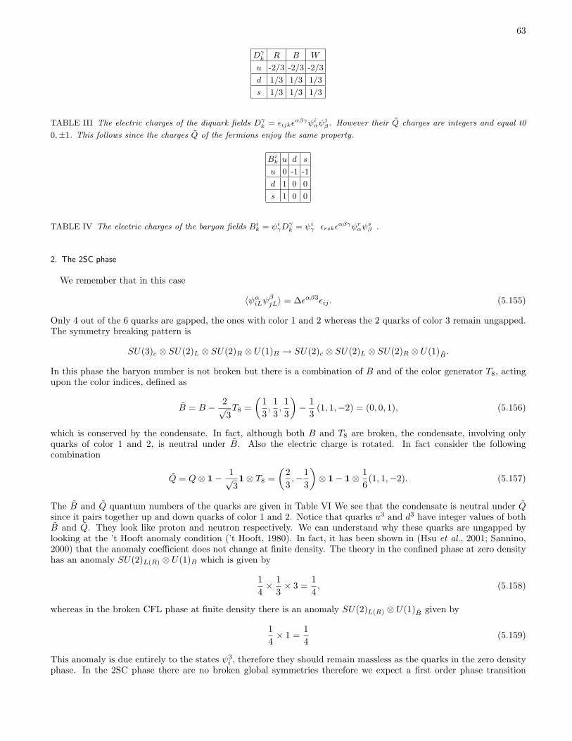
63
Dγk R B W
u -2/3 -2/3 -2/3
d 1/3 1/3 1/3
s 1/3 1/3 1/3
TABLE III The electric charges of the diquark fields Dγk = εijkεαβγψi
αψjβ. However their Q charges are integers and equal t0
0,±1. This follows since the charges Q of the fermions enjoy the same property.
Bik u d s
u 0 -1 -1
d 1 0 0
s 1 0 0
TABLE IV The electric charges of the baryon fields Bik = ψi
γDγk = ψi
γ
εrskεαβγψr
αψsβ
.
2. The 2SC phase
We remember that in this case
〈ψαiLψβ
jL〉 = ∆εαβ3εij . (5.155)
Only 4 out of the 6 quarks are gapped, the ones with color 1 and 2 whereas the 2 quarks of color 3 remain ungapped.The symmetry breaking pattern is
SU(3)c ⊗ SU(2)L ⊗ SU(2)R ⊗ U(1)B → SU(2)c ⊗ SU(2)L ⊗ SU(2)R ⊗ U(1)B .
In this phase the baryon number is not broken but there is a combination of B and of the color generator T8, actingupon the color indices, defined as
B = B − 2√3T8 =
(13,13,13
)− 1
3(1, 1,−2) = (0, 0, 1), (5.156)
which is conserved by the condensate. In fact, although both B and T8 are broken, the condensate, involving onlyquarks of color 1 and 2, is neutral under B. Also the electric charge is rotated. In fact consider the followingcombination
Q = Q⊗ 1− 1√31⊗ T8 =
(23,−1
3
)⊗ 1− 1⊗ 1
6(1, 1,−2). (5.157)
The B and Q quantum numbers of the quarks are given in Table VI We see that the condensate is neutral under Qsince it pairs together up and down quarks of color 1 and 2. Notice that quarks u3 and d3 have integer values of bothB and Q. They look like proton and neutron respectively. We can understand why these quarks are ungapped bylooking at the ’t Hooft anomaly condition (’t Hooft, 1980). In fact, it has been shown in (Hsu et al., 2001; Sannino,2000) that the anomaly coefficient does not change at finite density. The theory in the confined phase at zero densityhas an anomaly SU(2)L(R) ⊗ U(1)B which is given by
14× 1
3× 3 =
14, (5.158)
whereas in the broken CFL phase at finite density there is an anomaly SU(2)L(R) ⊗ U(1)B given by
14× 1 =
14
(5.159)
This anomaly is due entirely to the states ψ3i , therefore they should remain massless as the quarks in the zero density
phase. In the 2SC phase there are no broken global symmetries therefore we expect a first order phase transition

64
Gik u d s
u 0 -1 -1
d 1 0 0
s 1 0 0
TABLE V The electric charges of the vector meson fields Gik = (D∗)i
αgαβ Dβ
k .
Q B
uα, α = 1, 2 12
0
dα, α = 1, 2 − 12
0
u3 1 1
d3 0 1
TABLE VI The electric charge (Q) and the baryon number (B) for the quarks in the CFL phase
to the nuclear matter phase with a competition between chiral and di-fermion condensates. Notice that there is nosuperfluidity in the 2SC phase.
The spectrum of the 2SC phase
We have already discussed the fermionic part, the modes ψαi with α = 1, 2 are gapped, whereas ψ3
i remain massless.Since the gauge group SU(3)c is broken down to SU(2)c we get
8− 3 = 5 (5.160)
massive gluons. However we have still 3 massless gluons belonging to the confining gauge group SU(2)c. With respectto this group the gapped fermions ψα
i with α = 1, 2 are confined, whereas the massless fermions ψ3i are un-confined.
Notice also that the electric charges of the confined states are not integers whereas the ones of the un-confined statesare integers.
As in 2SC no global symmetries are broken, there are no massless NG bosons. In conclusion the only light degreesof freedom are 3 gluons and 2 fermions.
3. The case of 2+1 flavors
In nature the strange quark is much heavier than the other two and it may happen that µ ≈ ms with µ À mu,d.In this situation neither of the discussions above applies. In practice we expect that decreasing µ from µ À mu,d,s
the system undergoes a phase transition from CFL to 2SC for values of µ in between ms and md,u. This is becausethe Fermi momenta of the different Fermi spheres get separated. In fact remember that for massive quarks the Fermimomentum is defined by the equation
EF = µ =√
p2F + M2 → pF =
√µ2 −M2. (5.161)
As a consequence the radius of the Fermi sphere of a given quark decreases increasing its mass. To see why such atransition is expected, let us consider a simplified model with two quarks, one massless and the other one with massms at the same chemical potential µ. The Fermi momenta are
pF1 =√
µ2 −m2s, pF2 = µ. (5.162)
The grand potential for the two unpaired fermions is (factor 2 from the spin degrees of freedom)
Ωunpair. = 2∫ pF1
0
d3p
(2π)3
(√~p 2 + m2
s − µ
)+ 2
∫ pF2
0
d3p
(2π)3(|~p | − µ) . (5.163)

65
In fact, the grand potential is given in general by the expression
Ω = −T∑
k
log∑nk
(e(µ−εk)/T
)nk
= −T∑
k
log(1 + e(µ−εk)/T
), (5.164)
where εk is the energy per particle and nk is the occupation number of the mode k. The expression above refers tofermions. Also
∑
k
→ gV
∫d3p
(2π)3, (5.165)
with g the degeneracy factor. In the limit of T → 0 and in the continuum we get
Ω = gV
∫d3p
(2π)3(εp − µ)θ(µ− εp). (5.166)
In order to pair the two fermions must reach some common momentum pFcomm, and the corresponding grand potential
can be written as
Ωpair. = 2∫ pF
comm
0
d3p
(2π)3(√
p 2 + m2s − µ
)+ 2
∫ pFcomm
0
d3p
(2π)3(|p | − µ)
− µ2∆2
4π2, (5.167)
where the last term is the energy necessary for the condensation of a fermion pair, that we recall from Eq. (3.65) tobe given by
−14ρ∆2 = −1
4p2
F
π2vF∆2 = −µ2∆2
4π2. (5.168)
This expression can be adapted to the present case by neglecting terms of order m2s∆
2. The common momentumpFcomm can be determined by minimizing Ωpair. with respect to pF
comm, with the result
pFcomm = µ− m2
s
4µ. (5.169)
It is now easy to evaluate the difference Ωunpair. − Ωpair. at the order m4s, with the result
Ωpair. − Ωunpair. ≈ 116π2
(m4
s − 4∆2µ2). (5.170)
We see that in order to have condensation the condition
µ >m2
s
2∆(5.171)
must be realized. Therefore if ms is too large the pairing does not occur. It is easy to see that the transition must befirst order. In fact if it were second order the gap ∆ should vanish at the transition, but in order this to happen wemust have ∆ > m2
s/2µ. It should be noticed that the value of ms appearing in this equations should be considereddensity dependent. For ms ≈ 200÷300 MeV and chemical potentials interesting for compact stellar objects (see later)the situation is shown in Fig. 20. We see that the gap should be larger than 40÷ 110 MeV in order to get the CFLphase, whereas for smaller value we have the 2SC phase. These values of ∆ are very close to the ones that one getsfrom the gap equation. Therefore we are not really able to judge if quark matter with the values of the parametersis in the CFL or in the 2SC phase. The situation is far more complicated, because differences in the Fermi momentacan be generated also from different chemical potentials (arising from the requirement of weak equilibrium, see later)and/or from the requirement of electrical and color neutrality as appropriated for compact stars. Furthermore, atthe border of this transition a crystalline phase, the so-called LOFF phase, can be formed. We will discuss all thesequestions later on.

66
220 240 260 280 300
50
60
70
80
90
100
110
= 400 MeVµ
= 500 MeVµ
∆ (MeV)
sM (MeV)
FIG. 20 The minimal values of the gap in order to get pairing for two given values of µ vs. ms.
4. Single flavor and single color
According to the values of the parameters single flavor and/or single color condensation could arise. A completelist of possibilities has been studied in (Alford et al., 2003) (for a review see (Bowers, 2003)). In general a single flavorcondensate will occur in a state of angular momentum J = 1. In this case rotational invariance is not broken since thecondensate is in an antisymmetric state of color 3∗ and and rotations and color transformations are locked together
〈sασβsγ〉 = ∆εαβγ , (5.172)
where σα is a spin matrix. This condensate breaks SU(3) ⊗ O(3) down to O(3). However, it is a general statementthat condensation in higher momentum states than J = 0 gives rise to smaller gaps, mainly due to a less efficient useof the Fermi surface. The typical gaps may range from 10 to 100 keV . We will not continue here this discussion.
In (Rajagopal and Wilczek, 2001) it is possible to find a discussion of many other possibilities as Nf > 3, the caseof two colors (of interest because it can be discussed on the lattice) and the limit Nf →∞.
VI. EFFECTIVE LAGRANGIANS
In this Section we will derive the effective lagrangians relevant to the two phases CFL and 2SC. The approach willbe the classical one, that is looking at the relevant degrees of freedom at low energy (with respect to the Fermi energy)and constructing the corresponding theory on the basis of the symmetries.
A. Effective lagrangian for the CFL phase
We will now derive the effective lagrangian for the light modes of the CFL phase. As we have seen such modesare the NG bosons. We will introduce the Goldstone fields as the phases of the condensates in the (3, 3) channel(Casalbuoni and Gatto, 1999; Hong et al., 1999) (remember also the discussion made in Section V.D)
Xiα ≈ εijkεαβγ〈ψj
βLψkγL〉∗, Y i
α ≈ εijkεαβγ〈ψjβRψk
γR〉∗. (6.1)
Since quarks belong to the representation (3,3) of SU(3)c ⊗ SU(3)L(R) they transform as (gc ∈ SU(3)c, gL(R) ∈SU(3)L(R))
ψL → ei(α+β)gcψLgTL , ψR → ei(α−β)gcψRgT
R, eiα ∈ U(1)B , eiβ ∈ U(1)A, (6.2)
whereas the transformation properties of the fields X and Y under the total symmetry group G = SU(3)c⊗SU(3)L⊗SU(3)R ⊗ U(1)B ⊗ U(1)A are
X → gcXgTLe−2i(α+β), Y → gcY gT
Re−2i(α−β). (6.3)

67
The fields X and Y are U(3) matrices and as such they describe 9 + 9 = 18 fields. Eight of these fields are eatenup by the gauge bosons, producing eight massive gauge particles. Therefore we get the right number of Goldstonebosons, 10 = 18− 10. In this Section we will treat the field associated to the breaking of U(1)A as a true NG boson.However, remember that this is a massive particle with a light mass at very high density. These fields correspond tothe breaking of the global symmetries in G = SU(3)L ⊗ SU(3)L ⊗ U(1)L ⊗ U(1)R (18 generators) to the symmetrygroup of the ground state H = SU(3)c+L+R ⊗ Z2 ⊗ Z2 (8 generators). For the following it is convenient to separatethe U(1) factors in X and Y defining fields, X and Y , belonging to SU(3)
X = Xe2i(φ+θ), Y = Y e2i(φ−θ), X, Y ∈ SU(3). (6.4)
The fields φ and θ can also be described through the determinants of X and Y
dX = det(X) = e6i(φ+θ), dY = det(Y ) = e6i(φ−θ), (6.5)
The transformation properties under G are
X → gcXgTL , Y → gcY gT
R, φ → φ− α, θ → θ − β. (6.6)
The breaking of the global symmetry can be discussed in terms of gauge invariant fields given by dX , dY and
Σij =
∑α
(Y jα )∗Xi
α → Σ = Y †X. (6.7)
The Σ field describes the 8 Goldstone bosons corresponding to the breaking of the chiral symmetry SU(3)L⊗SU(3)R,as it is made clear by the transformation properties of ΣT , ΣT → gLΣT g†R. That is ΣT transforms as the usual chiralfield. The other two fields dX and dY provide the remaining Goldstone bosons related to the breaking of the U(1)factors.
In order to build up an invariant lagrangian, it is convenient to define the following currents
JµX = XDµX† = X(∂µX† + X†gµ) = X∂µX† + gµ,
JµY = Y DµY † = Y (∂µY † + Y †gµ) = Y ∂µY † + gµ, (6.8)
with
gµ = igsgaµT a (6.9)
the gluon field and
T a =λa
2(6.10)
the SU(3)c generators. These currents have simple transformation properties under the full symmetry group G:
JµX,Y → gcJ
µX,Y g†c . (6.11)
The most general lagrangian, up to two derivative terms, invariant under G, the rotation group O(3) (Lorentzinvariance is broken by the chemical potential term) and the parity transformation, defined as:
P : X ↔ Y , φ → φ, θ → −θ, (6.12)
is (Casalbuoni and Gatto, 1999)
L = −F 2T
4Tr
[(J0
X − J0Y )2
)]− αTF 2
T
4Tr
[(J0
X + J0Y )2
)]+
12(∂0φ)2 +
12(∂0θ)2
+F 2
S
4Tr
[|JX − JY |2
]+ αS
F 2S
4Tr
[|JX + JY |2
]− v2
φ
2|∇φ|2 − v2
θ
2|∇θ|2.
or
L = −F 2T
4Tr
[(X∂0X
† − Y ∂0Y†)2
)]− αT
F 2T
4Tr
[(X∂0X
† + Y ∂0Y† + 2g0)2
)]
+F 2
S
4Tr
[∣∣∣X∇X† − Y ∇Y †∣∣∣2]
+ αSF 2
S
4Tr
[∣∣∣X∇X† + Y ∇Y † + 2g∣∣∣2]
+12(∂0φ)2 +
12(∂0θ)2 −
v2φ
2|∇φ|2 − v2
θ
2|∇θ|2. (6.13)

68
Using SU(3)c color gauge invariance we can choose X = Y †, making 8 of the Goldstone bosons disappear and givingmass to the gluons. The properly normalized Goldstone bosons, Πa, are given in this gauge by
X = Y † = eiΠaT a/FT , (6.14)
and expanding Eq. (6.13) at the lowest order in the fields we get
L ≈ 12(∂0Πa)2 +
12(∂0φ)2 +
12(∂0θ)2 − v2
2|∇Πa|2 − v2
φ
2|∇φ|2 − v2
θ
2|∇θ|2, (6.15)
with
v =FS
FT. (6.16)
The gluons ga0 and ga
i acquire Debye and Meissner masses given by
m2D = αT g2
sF 2T , m2
M = αSg2sF 2
S = αSg2sv2F 2
T . (6.17)
It should be stressed that these are not the true rest masses of the gluons, since there is a large wave functionrenormalization effect making the gluon masses of order of the gap ∆, rather than µ (see later) (Casalbuoni et al.,2001c,d). Since this description is supposed to be valid at low energies (we expect much below the gap ∆), we couldalso decouple the gluons solving their classical equations of motion neglecting the kinetic term. The result from Eq.(6.13) is
gµ = −12
(X∂µX† + Y ∂µY †
). (6.18)
It is easy to show that substituting this expression in Eq. (6.13) one gets
L =F 2
T
4
(Tr[ΣΣ†]− v2Tr[~∇Σ · ~∇Σ†]
)+
12
(φ2 − v2
φ|~∇φ|2)
+12
(θ2 − v2
φ|~∇θ|2)
. (6.19)
Notice that the first term is nothing but the chiral lagrangian except for the breaking of the Lorentz invariance. Thisis a way of seeing the quark-hadron continuity, that is the continuity between the CFL and the hypernuclear matterphase in three flavor QCD discussed previously. Furthermore one has to identify the NG φ associated to the breakingof U(1)B with the meson H of the hypernuclear phase (Schafer and Wilczek, 1999a).
B. Effective lagrangian for the 2SC phase
In Section V.D.2 we have seen that the only light degrees of freedom in the 2SC phase are the u and d quarks ofcolor 3 and the gluons belonging to the unbroken SU(2)c. The fermions are easily described in terms of ungappedquasi-particles at the Fermi surface and we will not elaborate about these modes further. In this Section we will discussonly the massless gluons. An effective lagrangian describing the 5 would-be Goldstone bosons and their couplingsto the gluons has been given in (Casalbuoni et al., 2000). The effective lagrangian for the massless gluons has beengiven in (Rischke et al., 2001) and it can be obtained simply by noticing that it should be gauge invariant. Thereforeit depends only on the field strengths
Eai = F a
0i, Bai =
12εijkF a
jk, (6.20)
where F aµν is the usual non-abelian curvature. As we know, Lorentz invariance is broken, but rotations are good
symmetries, therefore the most general effective lagrangian we can write at the lowest order in the derivatives of thegauge fields is
Leff =1g2
3∑a=1
(ε
2Ea ·Ea − 1
2λBa ·Ba
). (6.21)
The constants ε and λ have the meaning of the dielectric constant and of the magnetic permeability. The speed ofthe gluons turns out to be given by
v =1√ελ
. (6.22)

69
We will see later how to evaluate these constants starting from the HDET but we can see what are the physicalconsequences of this modification of the usual relativistic lagrangian. The most interesting consequence has to dowith the Coulomb law and the effective gauge coupling. In fact, as we shall see, at the lowest order in 1/µ expansion,λ = 1. The Coulomb potential between two static charges get modified
VCoul =g2
εr=
g2eff
r, g2
eff =g2
ε. (6.23)
Furthermore, the value of αeffs , reintroducing the velocity of light c, and keeping h/ = 1 is
αs =g2
4πc→ α′s =
g2eff
4πv=
g2
4πc√
ε. (6.24)
If, as it is the case, ε is much bigger than 1, the gluons move slowly in the superconducting medium and
α′sαs
=1√ε¿ 1. (6.25)
Therefore the effect of the medium is to weaken the residual strong interaction. The same result can be obtained byperforming the following transformation in time, fields and coupling:
x0′ =x0
√ε, Aa′
0 =√
εAa0 , g′ =
g
ε1/4. (6.26)
The effective lagrangian takes the usual form for a relativistic gauge theory in terms of the new quantities
Leff = − 14g′2
F a′µνFµνa′ , (6.27)
with
F a′µν = ∂
′µAa′
ν − ∂′νAa′
µ + fabcAb′µ Ac′
ν . (6.28)
The calculation shows (Casalbuoni et al., 2002d; Rischke, 2000; Rischke et al., 2001) that
ε = 1 +g2µ2
18π2∆2≈ g2µ2
18π2∆2, (6.29)
since typically ∆ ¿ µ. We recall also that at asymptotic values of µ the calculations from QCD show that (see SectionV.C)
∆ = cµg−5e−3π2/√
2g. (6.30)
Using Eqs. (6.29) and (6.24) we obtain
α′s =3
2√
2g∆µ
. (6.31)
This is the way in which the coupling gets defined at the matching scale, that is at ∆. Since SU(2) is an asymptoticallyfree gauge theory, going at lower energies makes the coupling to increase. The coupling gets of order unity at a scaleΛ′QCD. Since the coupling at the matching scale is rather small it takes a long way before it gets of order one. As aconsequence Λ′QCD is expected to be small. From one-loop beta function we get
Λ′QCD ≈ ∆e−2π/β0α′s ≈ ∆exp
(−2√
2π
11µ
g∆
), (6.32)
where β0 is the first coefficient of the beta function. In SU(2) we have β0 = 22/3. Notice that it is very difficult togive a good estimate of Λ′QCD since it depends crucially on the value of c which is very poorly known. In fact differentapproximations give different values of c. In (Pisarski and Rischke, 2000a; Schafer and Wilczek, 1999c) it has beenfound
c = 512π4, (6.33)

70
whereas in (Brown et al., 2000c; Wang and Rischke, 2002)
c = 512π4 exp(−4 + π2
8
). (6.34)
Using ΛQCD = 200 MeV to get g and µ = 600 MeV one finds Λ′QCD = 10 MeV in the first case and Λ′QCD = 0.3 keV
in the second case. Although a precise determination of Λ′QCD is lacking, it is quite clear that
Λ′QCD ¿ ΛQCD. (6.35)
Notice also that increasing the density, that is µ, Λ′QCD decreases exponentially. Therefore the confinement radius1/Λ′QCD grows exponentially with µ. This means that looking at physics at some large, but fixed, distance andincreasing the density, there is a crossover density when the color degrees of freedom become deconfined.
VII. NGB AND THEIR PARAMETERS
In this Section we will evaluate the parameters appearing in the effective lagrangian for the NG bosons in the CFLphase. Furthermore we will determine the properties of the gluons in the 2SC phases. A nice way of organizing thiscalculation is to make use of the HDET which holds for residual momenta such that ∆ ¿ ` ¿ δ and to match, atthe scale ∆, with the effective lagrangian supposed to hold for momenta ` ¿ ∆. This calculation can be extendedalso to massive gluons both in CFL and in 2SC. However the expansion in momenta is not justified here, since thephysical masses turn out to be of order ∆. On the other hand by a numerical evaluation we can show that the erroris not more than 30%, and therefore this approach gives sensible results also in this case. The way of evaluating thepropagation parameters for NG bosons and for gluons is rather simple, one needs to evaluate the self-energy in bothcases. The self-energy for the gluons is not a problem since we know the couplings of the gluons to fermions. Howeverwe need the explicit expression of the interaction between NG bosons and quarks. This interaction can be easilyobtained since we know the coupling of the fermions to the gap and the phases of the gap are the NG boson fields.Therefore we need only to generalize the Majorana mass terms (the coupling with the gap) to an interaction with theNG bosons such to respect the total symmetry of the theory. We will illustrate the way of performing this calculationin the specific example of the NG boson corresponding to the breaking of U(1)B and we will illustrate the resultsfor the NG bosons. Before doing that we will derive first the lagrangians for the HDET in the CFL and in the 2SCphases. We have also to mention that the parameters of the NG bosons have been derived by many authors (Beaneet al., 2000; Hong et al., 2000a; Manuel and Tytgat, 2000, 2001; Rho et al., 2000a,b; Son and Stephanov, 2000a,b),although using different approaches from the one considered here (Casalbuoni et al., 2002d, 2001c,d).
A. HDET for the CFL phase
In the CFL phase the symmetry breaking is induced by the condensates
〈ψL Tαi CψL
βj〉 = −〈ψR Tαi CψR
βj〉 ≈ ∆ εαβIεijI , (7.1)
where ψL, R are Weyl fermions and C = iσ2. The corresponding Majorana mass term is given by (ψ ≡ ψL):
∆2
3∑
I=1
ψT−CεIψ+εI + (L → R) + h.c., (7.2)
with the 3× 3 matrices εI defined as in Eq. (5.133)
(εI)ab = εIab . (7.3)
Expanding the quark fields in the basis (5.128)
ψ± =1√2
9∑
A=1
λAψA± . (7.4)
and following Section V.B we get the effective lagrangian at the Fermi surface
LD =∫
dv4π
9∑
A,B=1
χA†( i
2Tr[λA V ·D λB ] −∆AB
−∆ABi2Tr[λA V ·D∗ λB ]
)χB + (L → R), (7.5)

71
where
∆AB =12
3∑
I=1
∆Tr[εIλTAεIλB ], (7.6)
and we recall from Section V.B that
∆AB = ∆AδAB , (7.7)
with
∆1 = · · · = ∆8 = ∆, (7.8)
∆9 = −2∆. (7.9)
The CFL free fermionic lagrangian assumes therefore the form:
LD =∫
dv4π
9∑
A=1
χA†(
iV · ∂ −∆A
−∆A iV · ∂)
χA + (L → R) . (7.10)
From this equation one can immediately obtain the free fermion propagator in momentum space
SAB(p) =δAB
V · ` V · `−∆2A
(V · ` ∆A
∆A V · `)
. (7.11)
We recall that the NG bosons have been described in terms of the fields X and Y of Eq. (6.1). Since we wantto couple the NG bosons with fermions in a G invariant way let us look at the transformation properties of the gapterm. We have
3∑
I=1
Tr[ψTLCεIψLεI ] →
3∑
I=1
Tr[gLψTLgT
c εIgcψLgTLεI ]. (7.12)
Using the following property, holding for any unitary 3× 3 matrix , g
gT εIg =3∑
J=1
εJg†JIdet[g], (7.13)
which follows from
εijkgii′gjj′gkk′ = εi′j′k′det[g], (7.14)
we get
3∑
I=1
Tr[ψTLCεIψLεI ] →
3∑
I,J,K=1
(gc)†JI(gL)†KITr[ψT
LεJψLεK ]. (7.15)
This expression shows not only that the gap term is invariant under the locked transformations g∗L = gc, but alsothat it could be made invariant modifying the transformation properties of the fermions by changing gT
L to g†c . Thisis simply done by using the matrices X and Y respectively for the left- and right- handed quarks
(ψLX†) → gc(ψLX†)g†c , (ψRY †) → gc(ψRY †)g†c . (7.16)
Therefore, the coupling of the left-handed Weyl spinors ψ’s to the octet of NG boson fields is:
∆2
∑
I=1,3
Tr[(ψ−X†)T CεI(ψ+X†)εI ] + (L → R) + h.c., (7.17)
Both X and Y have v.e.v. given by
〈X〉 = 〈Y 〉 = 1 (7.18)

72
and we shall use the gauge
X = Y † . (7.19)
The lagrangian giving the the coupling of the quarks to the external fields can be obtained from (7.5) and is given by
LD =∫
dv4π
9∑
A,B=1
χA†(
i V · ∂δAB −Ξ∗BA
−ΞAB i V · ∂δAB
)χB + (L → R), (7.20)
where
ΞAB =3∑
I=1
12∆Tr
[εI
(λAX†)T
εI
(λBX†)] =
=3∑
I=1
12∆
(Tr[λAX†λBX†] − Tr[λAX†] Tr[λBX†]
). (7.21)
One can now expand X in terms of the NGB fields
X = exp i
(λaΠa
2F
), a = 1, · · · , 8 , (7.22)
and obtain the 3-point χχΠ, and the 4-point χχΠΠ couplings. The result is, for the 3-point coupling
LχχΠ = − i
∫dv4π
∆F
8∑a=1
Πa
√6
[χ9†Γ0 χa + χa†Γ0 χ9
]−
−8∑
a,b,c=1
dabcχa†Γ0χ
bΠc
. (7.23)
and for the 4-point coupling
LχχΠΠ =∫
dv4π
43
8∑a=1
∆8F 2
χ9†Γ1 χ9 ΠaΠa
+3
√23
8∑
a,b,c=1
(∆
8F 2dabcχ
c†Γ1 χ9 ΠaΠb + h.c.)
+8∑
a,b,c,d=1
∆8F 2
habcdχc†Γ0 χdΠaΠb
, (7.24)
where we have defined
habcd = 28∑
p=1
(gcapgdbp + dcdpdabp) − 83δacδdb +
43δcdδab, (7.25)
with
gabc = dabc + ifabc (7.26)
and
Γ0 =(
0 +1−1 0
), Γ1 =
(0 11 0
). (7.27)
In the CFL case we have also the NG bosons associated to the breaking of the U(1) factors. Let us consider thefollowing fields
U = eiσ/fσ , V = eiτ/fτ , (7.28)

73
with
σ = fσφ, τ = fτθ, (7.29)
where φ and θ are the dimensionless U(1) fields transforming according to Eq. (6.6)7. Clearly under U(1)B andU(1)A groups we have
U → e−iαU, V → e−iβV, (7.30)
whereas
ψL → ei(α+β)ψL, ψR → ei(α−β)ψR. (7.31)
We can make invariant couplings with the fermions simply by taking the combinations
UV ψL, UV †ψR. (7.32)
As a result we get full invariant couplings to the NG bosons modifying the quantity ΞAB appearing in Eq. (7.20) asfollows:
ΞAB → ΞABU2V 2. (7.33)
B. HDET for the 2SC phase
For the two flavour case, which encompasses both the 2SC model and the existing calculation in the LOFF phase(see later) we follow a similar approach.
The symmetry breaking is induced by the condensates
〈ψL Tαi CψL
βj〉 = −〈ψR Tαi CψR
βj〉 ≈ ∆ εαβ3εij3 , (7.34)
corresponding to the invariant coupling (ψ ≡ ψL):
∆2
ψT−Cε ψ+ε − (L → R) + h.c. , (7.35)
where
ε = iσ2 . (7.36)
As in the previous Section we use a different basis for the fermion fields by writing
ψ+,αi =3∑
A=0
(σA)αi√2
ψA+ (i, α = 1, 2)
ψ+,31 = ψ4+
ψ+,32 = ψ5+ , (7.37)
where σA are the Pauli matrices for A = 1, 2, 3 and σ0 = 1.A different, but also convenient notation for the fields ψ+, αi, makes use of the following combination of λ matrices,
as follows
ψ+,αi =5∑
A=0
(λA)αi√2
ψA+ . (7.38)
The λA matrices are defined in terms of the usual λ matrices as follows:
λ0 =1√3λ8 +
√23λ0, λA = λA (A = 1, 2, 3), λ4 =
λ4−i5√2
, λ5 =λ6−i7√
2. (7.39)
7 The couplings fσ and fτ have dimension 1 in units of mass.

74
Proceeding as before the 2SC fermionic lagrangian assumes the form:
LD =∫
dv4π
5∑
A,B=0
χA†(
i2Tr[λA V ·D λB ] −∆AB
−∆ABi2Tr[λA V ·D∗ λB ]
)χB + (L → R) . (7.40)
Here
∆AB =∆2
Tr[ εσTAεσB ] (A, B = 0, ...3),
∆AB = 0 (A,B = 4, 5) . (7.41)
We now use the identity (g any 2× 2 matrix), analogous to (5.134):
εgT ε = g − Tr[g] ; (7.42)
and we obtain
∆AB = ∆AδAB (7.43)
where ∆A is defined as follows:
∆A = (−∆, +∆, +∆, +∆, 0, 0) . (7.44)
Therefore the effective lagrangian for free quarks in the 2SC model can be written as follows
LD =∫
dv4π
5∑
A=0
χA†(
iV · ∂ −∆A
−∆A iV · ∂)
χA + (L → R) . (7.45)
From this equation one can immediately obtain the free fermion propagator that in momentum space is still given by(7.11), with the ∆A given by (7.44).
C. Gradient expansion for the U(1) NGB in the CFL model and in the 2SC model
In order to illustrate the procedure of evaluating the self-energy of the NG bosons we will consider here the case ofthe NG boson associated with the breaking of U(1)B . In particular, we will get the first terms in the effective actionfor the NG bosons by performing an expansion in momenta, ` ¿ ∆. An expansion of this kind is also called gradientexpansion (see (Eguchi, 1976) for a very clear introduction).
To start with we consider the U(1)B NG boson within the CFL model. Therefore we can put to zero all the NGfields in the HDET lagrangian except for the field U = exp iσ/fσ. Correspondingly the quark lagrangian of Eq.(7.20)with the modification (7.33) becomes
LD =∫
dv4π
9∑
A=1
χA†(
iV · ∂ −∆A U† 2
−∆A U2 iV · ∂)
χA + (L → R) . (7.46)
At the lowest order in the field σ we have
Lσ ≈∫
dv4π
9∑
A=1
χA†∆A
02iσ
fσ+
2σ2
f2σ
−2iσ
fσ+
2σ2
f2σ
χA + (L → R) , (7.47)
which contains the couplings σχχ and σσχχ. Notice that σ does not propagate at tree level, however a non trivialkinetic term is generated by quantum corrections. To show this we consider the generating functional where we takeonly left-handed fields for simplicity. Also in this case we will make use of the replica trick to take into account thefact that χ and χ† are not independent variables. Therefore we will have to take the square root of the fermiondeterminant. In (Casalbuoni et al., 2001c,d) this was taken into account by dividing by a factor 2 the sum over thevelocities appearing in the fermionic loops
∫dv4π
→∫
dv8π
. (7.48)

75
The generating functional is
Z[σ] =∫DχDχ† exp
i
∫χ†Aχ
(7.49)
where we have introduced (omit the indices of the fields for simplicity)
A = S−1 +2iσ∆fσ
Γ0 +2σ2∆
f2σ
Γ1 (7.50)
and
Γ0 =(
0 +1−1 0
), Γ1 =
(0 11 0
). (7.51)
with S−1 the free propagator. Performing the integration over the Fermi fields we get
Z[σ] = (det[A])1/2 = e
12Tr[log A]
. (7.52)
Therefore
Seff (σ) = − i
2Tr[log A]. (7.53)
Evaluating the trace we get
− i T r log A = −i T r log S−1
(1 + S
2iσ∆fσ
Γ0 + S2σ2∆
f2σ
Γ1
)
= −i T r log S−1 − i
∞∑n=1
(−1)2n−1
n
(iS
2iσ∆fσ
iΓ0 + iS2 σ2∆
f2σ
iΓ1
)n
. (7.54)
This is a loop expansion. At the lowest order it produces the effective action
Seff =i
4Tr
∫dxdy
[i S(y, x)2iσ(x)∆
fσi Γ0
i S(x, y)2iσ(y)∆fσ
i Γ0
]
+i
2Tr
∫dx
[i S(x, x) 2∆ σ2(x)
f2σ
i Γ1
]. (7.55)
The two terms correspond to the diagrams in Fig. 21, i.e. the self-energy, Fig. 21 a), and the tadpole, Fig. 21 b).They can be computed by the following set of Feynman rules to provide Seff (σ) In momentum space the Feynmanrules are as follows:
1. For each fermionic internal line with momentum p, associate the propagator
iSAB(p) = iδABS(p) =i δAB
V · ` V · `−∆2A + iε
(V · ` ∆A
∆A V · `)
; (7.56)
a) b)
FIG. 21 One-loop diagrams. External lines represent the NG boson field σ. Full lines are fermion propagators.

76
2. Each vertex introduces a term iLint that can be obtained from the effective lagrangian; for example the σcouplings to quarks can be derived from (7.47);
3. For each internal momentum not constrained by the momentum conservation perform the integration
4πµ2
(2π)4
∫d2` =
µ2
4π3
∫ +δ
−δ
d`‖
∫ +∞
−∞d`0 ; (7.57)
4. A factor (−1) and a factor of 2 for each fermion loop to take into account the spin (L + R). Also a factor 1/2is necessary due to the replica trick. This 1/2 will be associated to the sum over the velocities
5. A statistical factor arising from the Wick theorem if needed.
The result of the calculation of the effective lagrangian in momentum space is as follows:
iLI = −212
µ2
4π3
12
∫dv4π
∑
A,B
∫d2`
× Tr
[iSAB(` + p)
2i∆Bσ
fσiΓ0iSBA(`)
2i∆Aσ
fσiΓ0
],
iLII = −2µ2
4π3
12
∫dv4π
∑
A,B
∫d2` Tr
[iSAB(`)
2∆Bσ2
f2σ
i Γ1
], (7.58)
corresponding to the two diagrams of Figs. 21 a) and 21 b) respectively. After some computation one has
iLeff (p) = iLI(p) + iLII(p) = −12
∫dv4π
∑
A
µ2∆2A
π3f2σ
×∫
d2`[ V · (` + p)σV · ` σ + V · (` + p)σV · `σ − 2∆2
Aσ2
DA(` + p)DA(`)− 2σ2
DA(`)
], (7.59)
where we have defined
DA(p) = V · p V · p−∆2A + iε . (7.60)
One can immediately notice that
LI(p = 0) + LII(p = 0) = 0 . (7.61)
This result implies that the scalar σ particle has no mass, in agreement with Goldstone’s theorem. To get the effectivelagrangian in the CFL model at the lowest order in the σ momentum we expand the function in p (|p| ¿ |∆) to get,in momentum space
iLeff (p) = −12
∫dv4π
∑
A
2µ2∆4A
π3f2σ
(V · p)σ(V · p)σ I2 , (7.62)
where we have defined
I2 =∫
d2`
D3A(`)
. (7.63)
This and other integrals can be found in Appendix B. In getting this result we have used also the fact∫
(V · `)2DA(`)3
=∫
(V · `)2DA(`)3
= 0. (7.64)
In fact, since the integral is convergent we can send the cutoff δ to ∞ and to use the Lorentz invariance in 2 dimensionsto prove that these integrals are proportional to V 2 = V 2 = 0. We have
I2 = − i π
2∆4A
. (7.65)

77
Therefore we get, in configuration space,
Leff (x) =9µ2
π2f2σ
12
∫dv4π
(V · ∂σ)(V · ∂σ) . (7.66)
Since
12
∫dv4π
V µV ν =12
1 0 0 00 − 1
3 0 00 0 − 1
3 00 0 0 − 1
3
µν
, (7.67)
we obtain
Leff (x) =9µ2
π2f2σ
12
((∂0σ)2 − v2
σ(~∇σ)2)
, (7.68)
with
v2σ =
13
. (7.69)
This kinetic lagrangian has the canonical normalization factor provided
f2σ =
9µ2
π2(CFL) , (7.70)
Therefore the effective lagrangian for the NGB σ particle is:
Leff =12
((∂0σ)2 − 1
3(~∇σ)2
)=
12f2
σ
(U U† − 1
3∇U ·∇U†
), (7.71)
We note that the value of the velocity (7.69) is a consequence of the average over the Fermi velocities and reflects thenumber of the space dimensions, i.e. 3. Therefore it is universal and we expect the same value in all the calculationsof this type.
In the case of the 2SC model there is no σ field since the baryon number is not broken. However, neglecting themass of the τ field one can perform the same kind of calculation by using the invariant coupling derived for the CFLcase. The final result differs from the CFL case only in the coefficient in front of (7.70) which reflects the number ofcolor-flavor gapped degrees of freedom, 9 in the CFL case and 4 in the 2SC case; therefore one has
f2τ =
4µ2
π2(2SC) , (7.72)
whereas the result (7.69), being universal, holds also in this case. The NGB effective lagrangian is still of the form(7.71). The NGB boson is, in this case, only a would-be NGB because the axial U(1) is explicitly broken, though thisbreaking is expected to be small at high µ since the instanton density vanishes for increasing µ. (Son et al., 2001).
D. The parameters of the NG bosons of the CFL phase
Using the Feynman rules given above and the interaction lagrangians (7.23) and (7.24) we get the effective lagrangianas follows:
Lkineff =
µ2(21− 8 ln 2)36π2F 2
12
8∑a=1
(ΠaΠa − 1
3|~∇Πa|2
). (7.73)
Comparing with the effective lagrangian in Eq. (6.19) we see that
F 2T = F 2 =
µ2(21− 8 ln 2)36π2
, v2 =13. (7.74)

78
Therefore the pion satisfy the dispersion relation
E =1√3|p|. (7.75)
We notice that the evaluation of FT could be done just computing the coupling of the pions to their currents. To thisend one has to compute the diagram of Fig. 22 (Casalbuoni et al., 2001c,d). The result is
〈0|Jaµ |Πb〉 = iFδabpµ, pµ =
(p0,
13p)
, (7.76)
with F the same evaluated before. This result is particularly interesting since it shows how the conservation of thecolor currents is realized through the dispersion relation of the pions. In fact
p · p = E2 − 13|p|2 = 0. (7.77)
Π
χ
Jµab
FIG. 22 The one-loop contribution to the coupling of the NG bosons (dotted line) to their currents (wavy line). The fermionsin the loop are represented by a solid line.
E. The masses of the NG bosons in the CFL phase
Up to now we have considered massless quarks. In this Section we want to determine the influence of mass termsat the level of NG bosons. Remember that the QCD mass terms have the structure
ψLMψR + h.c. (7.78)
where M is the quark mass matrix. In order to determine the structure of the NG boson masses it is convenient tothink to M as a field (usually called a spurion field) transforming in such a way that the expression (7.78) is invariant.Recalling the transformation properties (6.2) of quark fields
ψL → ei(α+β)gcψLgTL , ψR → ei(α−β)gcψRgT
R, eiα ∈ U(1)B , eiβ ∈ U(1)A, (7.79)
it follows that M transforms as
M → e2iβgLMg†R. (7.80)
In this Section we will make use of the U(3) fields
X → gcXgTLe−2i(α+β), Y → gcY gT
Re−2i(α−β). (7.81)
In this discussion the U(1)A symmetry will play an important role. We recall again that this symmetry is broken bythe anomaly but this breaking goes to zero in the high density limit. If, in particular, we consider the subgroup (Z2)A
we see that NG boson mass terms can be only even in the matrix M . Linear terms in M may arise only from thisbreaking which is suppressed by (ΛQCD/µ)8 (see discussion in Section V.D). In order to build up the most generalmass term for the NG bosons let us introduce the gauge invariant U(3) field
Σ = (Y †X)T = e4iθΣT , (7.82)
where θ is the U(1)A field and Σ was defined in (6.7). We have
Σ → e−4iβgLΣg†R. (7.83)

79
We recall also the other two gauge invariant fields defined in (6.5)
dX = det(X) = e6i(φ+θ), dY = det(Y ) = e6i(φ−θ), (7.84)
and transforming as
dX → e−6i(α+β)dX , dY → e−6i(α−β)dY . (7.85)
We have also
det(M) → e6iβdet(M), det(Σ) → e−12iβdet(Σ). (7.86)
Notice that since dX and dY are the only terms transforming under U(1)V , invariance requires that the effectivelagrangian should depend only on the combination
dXdY † = det(Σ). (7.87)
Other quantities that can be considered are
MΣ†, → e6iβgLMΣ†g†L, M†Σ → e−6iβgRM†Σg†RM−1Σ → e−6iβgRMΣ†g†R, M−1†Σ† → e6iβgLM−1†Σ†g†L. (7.88)
One can build terms transforming only with respecto to U(1)A by taking traces of these quantities. However, takinginto account the Cayley identity for 3× 3 matrices
A3 − Tr(A)A2 +12((Tr(A))2 − Tr(A2)) A− det (A) = 0, (7.89)
we see that multiplying this expression by A−1 and taking the trace we can express the trace of terms in the secondline of (7.88) as a combination of the trace of the terms in the first line, their second power and the determinants ofM and Σ. In the same way we see that it is enough to consider only the first and the second power of the terms inthe first line of (7.88). Summarizing, it is enough to take into considerations the following quantities
det(Σ), det(M), det(M†),
Tr[M Σ†], Tr[M†Σ], Tr[(M Σ†)2], Tr[(M†Σ)2]. (7.90)
Therefore the most general invariant term involving the quark mass matrix M is of the form
I = (det(Σ))a1(det(M))a2(det(M†))a2
×(Tr[M Σ†])a3(Tr[M†Σ])a3(Tr[(M Σ†)2])a4(Tr[(M†Σ)2])a4 . (7.91)
Requiring analyticity all the exponents must be integers. The term I is invariant under the full group except forU(1)A. Requiring also U(1)A invariance we get the equation
−2a1 + (a2 − a2) + (a3 − a3) + 2(a4 − a4) = 0. (7.92)
If we ask I to be of a given order n in the mass matrix we have also the condition
3(a2 + a2) + (a3 + a3) + 2(a4 + a4) = n. (7.93)
If we subtract these two equations one by another we find
2a1 + 4a2 + 2a2 + 2a3 + 4a4 = n, (7.94)
which implies that n must be even, as it should be by (Z2)A invariance alone. This argument shows also that the itwould be enough to require the invariance under the discrete axial group. If we now select n = 2 (the lowest powerin the mass), Eq. (7.93) implies
a2 = a2 = 0. (7.95)

80
Therefore the only solutions to our conditions are
a1 = 1, a3 = 2, a3 = 0, a4 = 0, a4 = 0a1 = 1, a3 = 0, a3 = 0, a4 = 1, a4 = 0 (7.96)a1 = 0, a3 = 1, a3 = 1, a4 = 0, a4 = 0 .
If the matrix M has no zero eigenvalues we can use the Cayley identity to write a linear combination of the first twosolutions in the following form
Tr[M−1Σ]det(M) =12det(Σ)
(Tr[M Σ†]
)2
− Tr[(MΣ†)2]
. (7.97)
In conclusion the most general invariant term is given by
Lmasses = −c(det(M)Tr[M−1Σ] + h.c.
)− c′
(det(Σ)Tr[(M Σ†)2] + h.c.
)
−c′′(Tr[M Σ†]Tr[M†Σ]
). (7.98)
The coefficients appearing in this expression can be evaluated by using the matching technique (Beane et al., 2000;Hong et al., 2000a; Rho et al., 2000b; Son and Stephanov, 2000a,b) (see also the review paper (Schafer, 2003)). Theidea is to evaluate the contribution of Lmasses to the vacuum energy. One starts evaluating an effective four-fermiinteraction due to a hard gluon exchange and performing a matching between QCD and HDET as illustrated in Fig.23. The contribution from QCD arises from a double chirality violating process producing a contribution proportionalto the square of the masses (Schafer, 2002).
L
L L
L R
R
M
MM
2
L
L
R
R
FIG. 23 The effective four-fermi interaction produced by a chirality violating process in QCD. There are other contributionsobtained by exchanging the points where the gluon line is attached with the mass insertions.
Then one uses this effective interaction in HDET to evaluate the contribution to the vacuum energy to be matchedagainst the contribution from Lmasses obtained by putting Σ = 1 (the vacuum state). This is illustrated in Fig. 24.
MML R
FIG. 24 The effective four-fermi interaction of Fig. 23 is used to evaluate the contribution to the vacuum energy of the termsproportional to M2.
The result of this computation is
c =3∆2
2π2, c′ = c′′ = 0. (7.99)

81
There is a simple way of understanding why only the c contribution survives at the leading order. In fact, this is theonly term which arises working at the second order in perturbation theory and approximating the product of Fermifields with the corresponding NG fields X and Y . We find
(ψLMψR)2 = (ψi†LαM j
i ψαRj)(ψ
k†LβM l
kψβRl) ≈ εikmεαβγXγ
mM ji M l
kεjlpεαβδY p∗
δ
≈ εikmεjlpMji M l
kΣpm = εikmεjlpM
ji M l
kMam(M−1)b
aΣpb ≈ det(M)Tr[M−1Σ]. (7.100)
There is also another interesting point about the quark masses. Starting from the complete QCD lagrangian
LQCD = ψ(iD/ + µγ0)ψ − ψLMψR − ψRM†ψL − 14Ga
µνGµνa (7.101)
and repeating what we did in Section V.B for deriving the HDET expansion we find that at the leading order theexpression for the negative energy left-handed fields is
ψ−,L =12µ
(−iγ0D/ ⊥ψ+,L + γ0Mψ+,R
). (7.102)
Substituting inside the lagrangian one finds (we neglect here the condensate terms for simplicity)
LD = ψ†+,L(iV ·D)ψ+,L − 12µ
ψ†+,L
[(D/ ⊥)2 + MM†] ψ+,L + (L ↔ R, M ↔ M†) + · · · . (7.103)
The new term that we have obtained is just what expected from the expansion of the kinetic energy of the quark. Wesee that the mass terms in the effective lagrangian behave as effective chemical potentials. Notice that in presence ofa chemical potential a Dirac lagrangian has the form
ψiγν(∂ν − iµgν0)ψ, (7.104)
therefore the chemical potential acts as the fourth component of an abelian gauge field. This implies that thelagrangian is invariant under the gauge transformation
ψ → eiα(t)ψ, µ → µ + α(t). (7.105)
This argument implies that the HDET lagrangian has the invariance8
ψL → L(t)ψL, ψR → R(t)ψR, (7.106)
where L(t) and R(t) are time dependent flavor transformation and with
XL =12µ
MM†, XR =12µ
M†M (7.107)
transforming as left- and right- handed gauge fields (Bedaque and Schafer, 2002). But then also the effective lagrangianfor the filed Σ has to satisfy this symmetry, meaning that we should substitute the time derivative with the covariantderivative
∂0Σ → ∇0Σ = ∂0Σ + iΣ(
MM†
2µ
)T
− i
(M†M
2µ
)T
Σ, (7.108)
where we have taken into account that
MM† → gLMM†g†L, M †M → gRM†Mg†L, Σ → g∗RΣgTL . (7.109)
This result has been confirmed by a microscopic calculation done in (Bedaque and Schafer, 2002). We can now seethat a generic term in the expansion of the effective lagrangian has the form
F 2∆2
(∂0 − iMM†/(2µ)
∆
)n (∇∆
)m (M2
F 2
)p
(Σ)q(Σ†)r. (7.110)
8 Notice that D/ ⊥ does not involve time derivatives.

82
The various terms are easily understood on the basis of the fact that the momentum expansion is a series in p/∆.The factor ∆2 in front is just to adjust the normalization of the kinetic terms arising for n = 2 and m = 0 andn = 0, m = 2, with q = r = 1. The term quadratic in the mass matrix, M , has also the correct normalization. Wenow see that the contribution to the square masses of the mesons of the masses originating from the kinetic energyexpansion and the ones coming from the explicit quark mass terms might be of the same order of magnitude. In fact,the contribution to the NG bosons square masses are (the extra 1/F 2 terms originate from the expansion of Σ)
kinetic energy : F 2∆2 m4
µ2∆2
1F 2
≈ m4
µ2,
quark masses : F 2∆2 m2
F 2
1F 2
≈ ∆2m2
F 2, (7.111)
and the two contributions are of the same order of magnitude for m ≈ ∆, since F ≈ µ. Before studying the massspectrum we will now introduce another subject which is relevant to the physics of the NG bosons of the CFL phase,that is the subject of Boson-Einstein condensation.
1. The role of the chemical potential for scalar fields: Bose-Einstein condensation
Let us consider a relativistic complex scalar field (however similar considerations could be done for the non-relativistic case) described by the lagrangian density
∂µφ†∂µφ−m2ψ†φ− λ(φ†φ)2. (7.112)
The quartic term gives rise to a repulsive interaction for λ > 0 as it is required by the stability of theory. Thelagrangian has a phase symmetry U(1) giving rise to a conserved current. A simple way of introducing the chemicalpotential is to notice that we can promote the global U(1) to a local one by adding a gauge field. However, bydefinition
∂L∂Aµ
= −jµ, (7.113)
and therefore the charge density is obtained by varying the lagrangian with respect to the fourth component of thegauge potential. But in a system at finite density the variation with respect to the chemical potential is just thecorresponding conserved charge, therefore the chemical potential must enter in the lagrangian exactly as the fourthcomponent of a gauge field. Therefore we get
L = (∂0 + iµ)φ†(∂0 − iµ)φ− (∇φ†) · (∇φ)−m2φ†φ− λ(φ†φ)2
= ∂µφ†∂µφ− (m2 − µ2)φ†φ− λ(φ†φ)2 + iµ(φ†∂0φ− ∂0φ†φ). (7.114)
Notice that the last term breaks the charge conjugation symmetry of the theory since µ multiplies the charge density.As a result the mass spectrum is given by
p2 − (m2 − µ2) + 2µQp0 = 0, (7.115)
where Q = ±1 is the charge for particles and antiparticles. The dispersion relation can be written as
(E + µQ)2 = m2 + |p|2 (7.116)
with E = p0. We see that the mass of particles and antiparticles are different and given by
mp,p = ∓µ + m. (7.117)
This is what happens if µ2 < m2. At µ2 = m2 the system undergoes a second order phase transition and a condensateis formed. The condensate is obtained by minimizing the potential
V (φ) = (m2 − µ2)φ†φ + λ(φ†φ)2, (7.118)
from which
〈φ†φ〉 =µ2 −m2
2λ. (7.119)

83
Notice also that at µ = m the mass of the particle mode goes to zero. In correspondence of the condensation thesystem has a charge density given by
ρ = −∂V
∂µ= 2µ〈φ†φ〉 =
µ
λ(µ2 −m2). (7.120)
Therefore the ground state of the system is a Bose-Einstein condensate. Defining
〈φ〉 =v√2, v2 =
µ2 −m2
λ, (7.121)
we can derive the physical spectrum of the system through the replacement
φ(x) =1√2(v + h(x))eiθ(x)/v. (7.122)
The quadratic part of the lagrangian is
L2 =12∂µθ∂µθ +
12∂µh∂µh− λv2h2 − 2µh∂0θ. (7.123)
The mass spectrum is given by the condition
det(
p2 − 2λv2 2iµE−2iµE p2
)= 0. (7.124)
At zero momentum we get (pµ = (M,0))
M2(M2 − 2λv2 − 4µ2) = 0. (7.125)
Therefore the antiparticle remains massless after the transition, whereas the particle gets a mass given by
M2 = 6µ2 − 2m2. (7.126)
At the transition point these two masses agree with the ones in the unbroken phase, Eq. (7.117). The masses in thetwo phases are illustrated in Fig. 25.
M
m
m
µ
massive mode
Goldstone mode
broken phasenormalphase
m2
FIG. 25 This figure shows the evolution of the particle and antiparticle masses from the normal phase to the broken one.
It is interesting to find out the energies of these particles in the small momentum limit. We find for the Goldstonemode
ENG ≈√
µ2 −m2
3µ2 −m2|p|, (7.127)

84
whereas for the massive one
Emassive ≈√
6µ2 − 2m2 +9µ2 −m2
6µ2 − 2m2|p|2. (7.128)
The velocity of the Goldstone mode is particularly interesting since it is zero at the transition point and goes to 1/√
3at large densities. Remember that this is just the velocity we have found in our effective lagrangian describing theNG bosons in the CFL phase.
2. Kaon condensation
Starting from the mass terms for the NG bosons of the CFL phase obtained in Section VII.E one can easilyunderstand the results for the masses of the flavored NG bosons
mπ± = ∓m2d −m2
u
2µ+
√2c
F 2(mu + md)ms,
mK± = ∓m2s −m2
u
2µ+
√2c
F 2(mu + ms)md,
mK0,K0 = ∓m2s −m2
d
2µ+
√2c
F 2(md + ms)mu. (7.129)
The two terms in this expression have their counterpart in Eq. (7.117). The first term arises from the ”chemicalpotential” terms MM†/2µ whereas the second term comes from the ”true” mass term. Also in this case a Bose-Einstein condensate might be formed. For simplicity consider the case ms À mu,md. Then we get
mπ± ≈ 1F
√2cms(mu + md),
mK± ≈ ∓m2s
2µ+
1F
√2cmsmd,
mK0,K0 ≈ ∓m2s
2µ+
1F
√2cmsmu. (7.130)
The pion masses are independent on the chemical potential terms, however the masses of K+ and K0 are pusheddown (whereas the ones of K− and K0 are pushed up) and therefore they become massless at
ms
∣∣∣crit
=(
12µ2
π2F 2
)1/33
√mu,d∆2 = 6
(2
21− 8 log 2
)1/33
√mu,d∆2 ≈ 3.03 3
√mu∆. (7.131)
The critical value of ms can vary between 41 MeV for mu = 1.5 MeV and ∆ = 40 MeV and 107 MeV formu = 4.5 MeV and ∆ = 100 MeV . For larger values of ms the modes K+ and K0 become unstable. This is thesignal for condensation (Bedaque and Schafer, 2002; Schafer, 2000a). In fact if we look for a kaon condensed groundstate of the type9
Σ = eiαλ4 = 1 + (cos α− 1)λ24 + iλ4 sinα, (7.132)
we obtain from our effective lagrangian, in the limit of exact isospin symmetry, (subtracting the term for α = 0) thepotential
V (α) = F 2
(−1
2
(m2
s
2µ
)2
sin2 α + (m0K)2(1− cos α)
), (7.133)
9 The most general ansatz would be to assume in the exponential a linear combination of λa, a = 4, 5, 6, 7, but it turns out that theeffective potential depends only on the coefficient of λ4. This is related to the fact that, as we shall see, there are three broken symmetriesand therefore there must be three flat directions in the potential.

85
where m0K is the lowest order square mass of the kaon in ms, that is
(m0K)2 =
2 cms m
F 2(7.134)
and m = mu = md. As in the example of a complex scalar field we see that the ”chemical potential” terms givea negative contribution, whereas the ”mass” terms gives a positive one. Therefore it is convenient to introduce theeffective chemical potential
µeff =m2
s
2µ. (7.135)
We see that
V (α) = F 2
(−1
2µ2
eff sin2 α + (m0K)2(1− cos α)
). (7.136)
Minimizing the potential we find a solution with α 6= 0, given by
cosα =(m0
K)2
µ2eff
(7.137)
if
µeff ≥ m0K . (7.138)
One can also derive the hypercharge density
nY = − ∂V
∂µeff= µeffF 2
(1− (m0
K)4
µ4eff
). (7.139)
The mass terms break the original SU(3)c+L+R symmetry of the CFL ground state to SU(2)I ⊗ U(1)Y . The kaoncondensation breaks this symmetry to the diagonal U(1) group generated by
Q =12
(λ3 − 1√
3λ8
). (7.140)
In fact, one can easily verify that
[Q, Σ] = 0. (7.141)
This result can be simply understood by the observation that under SU(2)I ⊗U(1)Y the NG bosons in Σ decomposeas a triplet, the pions, a complex doublet (K0, K
−) and its complex conjugate (K+,K0) and a singlet, η. The α 6= 0solution for Σ gives rise to an expectation value for the doublets. We see that the symmetry breaking mechanism isthe same as for the electroweak sector of the Standard Model (SM). Therefore SU(2)⊗U(1) is broken down to U(1)
Notice that by the usual counting of NG bosons one would expect 3 massless modes. However we have seen fromthe unbroken phase that only two modes become massless at the transition. This comes from the breaking of Lorentzinvariance due to the presence of the chemical potential in the original QCD lagrangian. A theorem due to Chadaand Nielsen (Nielsen and Chada, 1976) gives the key for the right counting of the NG physical bosons. The essenceof the theorem is that the number depends on the dispersion relation of the NG bosons. If the energy is linear inthe momentum (or a odd power) the counting is normal. If the energy depends on the momentum quadratically(or through an even power), then there are two broken generators associated to a single NG bosons. Notice that inrelativistic theories the dispersion relations are always of the first type. A more recent discussion of this topics is in(Miransky and Shovkovy, 2002; Schafer et al., 2001). In particular in (Schafer et al., 2001) it is proved a theoremwhich helps to show algebraically when the dispersion relations are odd or even in the momenta. The behavior of themasses with the effective chemical potential is represented in Fig. 26.
The effective lagrangian for the NG bosons in the CFL phase has been useful for the study of many phenomenologicalinteresting questions in the realm of compact stellar objects (Buckley and Zhitnitsky, 2002; Jaikumar et al., 2002;Kaplan and Reddy, 2002a,b; Reddy et al., 2003; Shovkovy and Ellis, 2002).
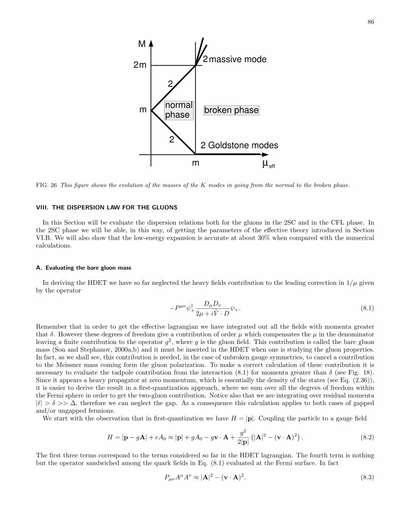
86
M
m
m
µ
massive mode
broken phasenormalphase
m22
2 Goldstone modes
2
2
eff
FIG. 26 This figure shows the evolution of the masses of the K modes in going from the normal to the broken phase.
VIII. THE DISPERSION LAW FOR THE GLUONS
In this Section will be evaluate the dispersion relations both for the gluons in the 2SC and in the CFL phase. Inthe 2SC phase we will be able, in this way, of getting the parameters of the effective theory introduced in SectionVI.B. We will also show that the low-energy expansion is accurate at about 30% when compared with the numericalcalculations.
A. Evaluating the bare gluon mass
In deriving the HDET we have so far neglected the heavy fields contribution to the leading correction in 1/µ givenby the operator
−Pµνψ†+DµDν
2µ + iV ·Dψ+. (8.1)
Remember that in order to get the effective lagrangian we have integrated out all the fields with momenta greaterthat δ. However these degrees of freedom give a contribution of order µ which compensates the µ in the denominatorleaving a finite contribution to the operator g2, where g is the gluon field. This contribution is called the bare gluonmass (Son and Stephanov, 2000a,b) and it must be inserted in the HDET when one is studying the gluon properties.In fact, as we shall see, this contribution is needed, in the case of unbroken gauge symmetries, to cancel a contributionto the Meissner mass coming form the gluon polarization. To make a correct calculation of these contribution it isnecessary to evaluate the tadpole contribution from the interaction (8.1) for momenta greater than δ (see Fig. 18).Since it appears a heavy propagator at zero momentum, which is essentially the density of the states (see Eq. (2.36)),it is easier to derive the result in a first-quantization approach, where we sum over all the degrees of freedom withinthe Fermi sphere in order to get the two-gluon contribution. Notice also that we are integrating over residual momenta|`| > δ >> ∆, therefore we can neglect the gap. As a consequence this calculation applies to both cases of gappedand/or ungapped fermions.
We start with the observation that in first-quantization we have H = |p|. Coupling the particle to a gauge field
H = |p− gA|+ eA0 ≈ |p|+ gA0 − gv ·A +g2
2|p|(|A|2 − (v ·A)2
). (8.2)
The first three terms correspond to the terms considered so far in the HDET lagrangian. The fourth term is nothingbut the operator sandwiched among the quark fields in Eq. (8.1) evaluated at the Fermi surface. In fact
PµνAµAν ≈ |A|2 − (v ·A)2. (8.3)

87
What we have to do now is just to sum over all the particles inside the Fermi sphere, which is equivalent to the tadpolecalculation. Notice that we should leave aside the fermions within the shell of momentum µ − δ < |p| < µ + δ, butthis give a negligible contribution since δ ¿ µ. Therefore we get
g2
2× 2×Nf ×
∫
|p|≤µ
d3p(2π)3
1|p|Tr
[A2 − (p ·A)2
|p|2]
, (8.4)
where the factors 2 and Nf comes from the spin and the number of flavors. On the other hand the trace is over thecolor indices. The result is simply
Nfg2µ2
6π2
12
∑a
Aa ·Aa. (8.5)
Therefore in the effective lagrangian of HDET we have to introduce a term
−12m2
D
∑a
Aa ·Aa (8.6)
with
m2BM = Nf
g2µ2
6π2. (8.7)
One could equally well perform this evaluation by using the Feynman rules for the heavy fields, which are easilyobtained, to determine the contribution to the polarization function Πab
µν . The contribution is the following
Πab BMµν = (−i)2× 2×Nf × (−1)
∫d`‖(2π)
(`‖ + µ)2
π
∫dv4π
∫d`02π
ig2δab
2(2µ + V · `)i
V · `Pµν . (8.8)
The different factors have the following origin. The first (−i) is due to the definition of Πµν such to reproduce themass term in the lagrangian. Then there is a factor 2 from the spin, a factor 2 from symmetry reasons (2 gluonfields). A factor Nf from the trace over the heavy fermions, a (−1) from the loop. We have left the residual momentaas integration variable, but the measure cannot be any more approximated as µ2 and we have put back the originalintegration factors. There is no extra 2 in the velocity integration since we have now no necessity of introducingthe Nambu-Gor’kov fields. The next factor arises from the vertex 2 gluons-2heavy fields and it is the result afterthe trace over the color indices. Finally we have the propagator of the ψh
+ field. If we define the propagator at zeromomentum as in Section II.A we get a contribution from the integral over `0 proportional to θ(−`‖) (see Eq. (2.38)).This restricts the integration over `‖ between −µ and 0. Performing the calculation one gets easily the result (8.7).In fact we have
Πab BMµν = −2iNfg2δab
∫ 0
−µ
d`‖2π
(`‖ + µ)2
π
12π
(2πi)2(`‖ + µ)
∫dv4π
Pµν =g2
2π2δab
µ2
2(−2
3δij)
= −m2BMδijδab. (8.9)
B. The parameters of the effective lagrangian for the 2SC case
We have now all the elements to evaluate the parameters appearing in the effective lagrangian for the 2SC case,which amounts to evaluate the propagation properties of the gluons belonging to the unbroken color group SU(2)c.We will need to evaluate the vacuum polarization function Πab
µν , a, b = 1, 2, 3, defined by the diagram in Fig. 27.
As usual we need the interaction term which is given by the coupling of the gauge field with the fermionic current
igAaµJµ
a . (8.10)
One finds
Jaµ =
∫dv4π
5∑
A,B=0
χA†(
i VµKAaB 00 −i VµK∗
AaB
)χB + (L → R) . (8.11)

88
g g
χ
FIG. 27 The Feynman diagram corresponding to the vacuum polarization of the gluons.
where we have used the basis (7.38) for the quark fields, leading to the coefficients KAaB
KAaB =14
TrλAλaλB = (K)AB . (8.12)
Using our Feynman rules we can compute Πabµν (Casalbuoni et al., 2002d)10. From the self energy diagram of Fig. 27
(a, b = 1, 2, 3) we find:
Πµν selfab (p) = 2× (−i)(−1)
∫dv8π
µ2
π
∫d2`
(2π)2( (igV µ)(igV ν)iV · ` iV · (` + p) + (V ↔ V )
D(` + p)D(`)+
− ∆2 (igV µ)(igV ν) + (igV ν)(igV µ)D(` + p)D(`)
)Tr[KaKb] . (8.13)
where
Tr[KaKb] = δab. (8.14)
In order to derive the effective lagrangian it is enough to expand this expression up to the second order in momentaand add the contribution from the bare Meissner mass. The result is (Casalbuoni et al., 2002d)
Π00ab(p) = δab
µ2g2
18π2∆2|~p |2 , (8.15)
Πklab(p) = Πkl self
ab + Πkl BMab = δabδ
kl µ2g2
3π2
(1 +
p20
6∆2
)− δabδ
kl µ2g2
3π2= δabδ
kl µ2g2
18π2
p20
∆2, (8.16)
Π0kab(p) = δab
µ2g2
18π2∆2p0pk . (8.17)
We see that the bare Meissner mass contribution Πkl BMab (p) just cancels the zero momentum contribution to the
gluon self-energy. As a consequence the unbroken gluons remain massless. These results agree with the outcomes of(Rischke, 2000; Rischke et al., 2001).
We notice also that there is no contribution to the Debye mass (the mass associated to the component Π00ab of the
vacuum polarization). This results reflects the fact that in the 2SC model the SU(2)c color subgroup generated bythe first three generators T c (c = 1, 2, 3) remains unbroken.
One can now compute the dispersion laws for the unbroken gluons. From the previous formulas one gets:
L = −14Fµν
a F aµν +
12Πµν
ab AaµAb
ν . (8.18)
Introducing the fields Eai ≡ F a
0i and Bai ≡ iεijkF a
jk, and using (8.15), (8.16) and (8.17) these results can be written asfollows (assuming gauge invariance the terms with 3 and 4 gluons are completely fixed, but see later):
L =12(Ea
i Eai −Ba
i Bai ) +
k
2Ea
i Eai , (8.19)
10 For the same calculation using different methods see: (Rischke, 2000; Rischke et al., 2001).

89
with
k =g2µ2
18π2∆2. (8.20)
These results have been first obtained in (Rischke et al., 2001). As discussed in this paper, these results imply thatthe medium has a very high dielectric constant ε = k + 1 and a magnetic permeability λ = 1. The gluon speed in thismedium is now
v =1√ελ∝ ∆
gµ(8.21)
and in the high density limit it tends to zero. We have already discussed the physical consequences of these results inSection VI.B.
In (Casalbuoni et al., 2002d) we have also computed the vacuum polarization of the gluons belonging to the brokenpart of the gauge group. That is the gluons with color index a = 4, 5, 6, 7, 8. In Table VII we give the results at zeromomentum in all the cases. These results are in agreement with a calculation performed by (Rischke, 2000) with a
a Π00(0) −Πij(0)
1− 3 0 0
4− 7 32m2
g12m2
g
8 3m2g
13m2
g
TABLE VII Debye and Meissner masses in the 2SC phase; m2g = µ2g2/3π2.
different method. In (Casalbuoni et al., 2002d) we have also made an expansion in momenta. A priori this expansioncannot be used to derive the dispersion relation for the broken gluons. In fact their mass, taking into account thewave function renormalization (of order g2µ2/∆2), is of order ∆. Defining the mass of the gluon as the value of theenergy at zero momentum one finds from the expansion
mR =√
2∆ (8.22)
for colors a = 4, 5, 6, 7, whereas the numerical calculation gives
mR = 0.894∆ (8.23)
and we see that the expansion overestimates the value of the mass. For the color 8 we find
mR =µg
π. (8.24)
The large value obtained of the mass for the gluon 8 in the small momentum expansion can be shown to be validat all orders in momentum. Except for the case a = 8 we see that generally there is a very large wave functionrenormalization making the physical gluon masses of order ∆ rather than of order gµ. This result was shown for thefirst time in (Casalbuoni et al., 2001c,d) in the case of the CFL phase. In (Casalbuoni et al., 2002d) the one-loopcontributions to the three and four gluon vertices has been evaluated. It has been checked that the result gives riseto the correct gauge invariant contribution when added to the tree level functions.
C. The gluons of the CFL phase
We will discuss here some of the results obtained in (Casalbuoni et al., 2001c,d) for the CFL case. We will skipmany technical details. We will only give the coupling of the currents to fermions which are again obtained from thegauge coupling. Working in the basis χA we use Eq. (7.5) to write
L1 = i g AµaJa
µ , (8.25)

90
where
Jaµ =
∫dv4π
9∑
A,B=1
χA†(
i VµhAaB 00 −i Vµh∗AaB
)χB + (L → R), (8.26)
and
hAaB =14
Tr[TAλaTB ] . (8.27)
Performing the trace we find
Jaµ =
i
2
√23
∑
~v
(χ9†
(Vµ 00 −Vµ
)χa + h.c.
)+
+i
2
∑
~v
8∑
b,c=1
χb†(
Vµgbac 00 −Vµg∗bac
)χc, (8.28)
where
gabc = dabc + ifabc . (8.29)
and dabc, fabc are the usual SU(3) symbols. The result of the self energy diagram (see Fig. 27) can be written asfollows:
i Πµν selfab (p) = −2
∫dv8π
∑
A,C,D,E
(−ig)2µ2
π
∫d2`
(2π)2Tr
[iSCD(` + p)×
×(
VνhDbE 00 −Vνh∗DbE
)iSEA(`)
(VµhAaC 0
0 −Vµh∗AaC
) ], (8.30)
where the propagator is given by Eq. (7.56). We note the minus sign on the r.h.s of (8.30), due to the presence of afermion loop and the factor 2 due to the spin (L + R). To this result one should add the contribution arising fromthe bare Meissner mass (see Eq. (8.7)):
Πµν BMab = − g2µ2
2π2δabδ
jkδµjδνk . (8.31)
To derive the dispersion law for the gluons, we write the equations of motion for the gluon field Abµ in momentum
space and high-density limit:
[(−p2gνµ + pνpµ)δab + Πνµ
ab
]Ab
µ = 0 . (8.32)
We define the rotational invariant quantities Π0, Π1,Π2 and Π3 by means of the following equations,
Πµν(p0, ~p) =
Π00 = Π0(p0, ~p)Π0i = Πi0 = Π1(p0, ~p) ni
Πij = Π2(p0, ~p) δij + Π3(p0, ~p)ninj
(8.33)
with n = p/|p| . It is clear that in deriving the dispersion laws we cannot go beyond momenta of order ∆, as the Fermivelocity superselection rule excludes gluon exchanges with very high momentum; it is therefore an approximation, butnevertheless a useful one, as in most cases hard gluon exchanges are strongly suppressed by the asymptotic freedomproperty of QCD.
By the equation
pνΠνµab Ab
µ = 0 , (8.34)
one obtains the relation
(p0 Π0 − |~p|Π1)A0 = ~n · ~A (p0 Π1 − |~p| (Π2 + Π3)) , (8.35)

91
between the scalar and the longitudinal component of the gluon fields. The dispersion laws for the scalar, longitudinaland transverse gluons are respectively
(Π2 + Π3 + p2
0
) (|~p|2 + Π0
)= p0|~p| (2Π1 + p0|~p|) ,(
Π2 + Π3 + p20
)(|~p| p0 + Π0) = p0|~p|
(2Π1 + p2
0
)+ Π2
1 ,
p20 − |~p|2 + Π2 = 0 . (8.36)
The analysis of these equations is rather complicated (Gusynin and Shovkovy, 2002) and we will give only the resultsarising from the expansion of the vacuum polarization up to the second order in momenta. The relevant expressionscan be found in (Casalbuoni et al., 2001c,d). The results at zero momentum are the same for all the gluons and theyare summarized in the Debye mass (from Π00) and in the Meissner mass (from Πii
m2D =
µ2g2
36π2(21− 8 ln 2) = g2F 2 , (8.37)
and
m2M =
µ2g2
π2
(−11
36− 2
27ln 2 +
12
)=
m2D
3, (8.38)
where the first two terms are the result of the diagram of Fig. 27, whereas the last one is the bare Meissner mass.These results agree with the findings of other authors as, for instance, (Son and Stephanov, 2000a,b; Zarembo, 2000).Recalling Eqs. (6.17)
m2D = αT g2F 2
T , m2M = αSv2g2F 2
T (8.39)
derived from the effective lagrangian for the CFL phase and the results already obtained for the parameters F 2T and
v2 we see that
αS = αT = 1. (8.40)
This completes the evaluation of the parameters of the effective lagrangian for the CFL phase.The Debye and Meissner masses do not exhaust the analysis of the dispersion laws for the gluons in the medium.
We will give here the result for the rest mass defined as the energy at zero momentum. Due to the large wave functionrenormalization, of order g2µ2/∆2, the rest mass turns out to be of order ∆. Precisely we find that for large valuesof µ one has
mRA ≈
mD√3α1
. (8.41)
with
α1 =µ2g2
s
216∆2π2
(7 +
163
ln 2)
. (8.42)
Therefore
mRA ≈
mD√3α1
=
√6
21− 8 ln 221 + 16 ln 2
∆ ≈ 1.70∆ . (8.43)
It is interesting to notice that the gluons are below threshold for the decay g → qq since in the CFL all the quarks aregapped with rest masses ∆ or 2∆. The rest mass can be also evaluated numerically without expanding in momenta.One finds
m ≡ mR = 1.36 ∆ . (8.44)
A comparison with (8.43) shows that the relative error between the two procedures is of the order of 20% and thisis also the estimated difference for the dispersion law at small ~p. We notice that also in this case the momentumexpansion approximation overestimates the correct result (Gusynin and Shovkovy, 2002).
The result about the large renormalization of the gluon fields can be easily understood by using the chiral expansionof Eq. (7.110) (Jackson and Sannino, 2003). To this end let us first notice that the renormalizion factor for the fieldsto be canonical is
gµ → gµ
∆gµ, (8.45)

92
which implies a coupling renormalization
g → ∆gµ
g =∆µ
. (8.46)
Therefore, after renormalization the coupling becomes ∆/µ. Now let us go back to the effective theory for the CFLphase and precisely to the equation used to decouple the gluon fields, Eq. (6.18)
gaµ = − 1
2g
(X∂µX† + Y ∂µY †
)≡ 1
gωa
µ. (8.47)
Now consider the kinetic term for the gluon fields∑
a
F aµνFµνa, (8.48)
with
F aµν = g∂µga
ν − ∂νgaµ − gfabcg
bµgc
ν (8.49)
and fabc the structure constants of the gauge group. Substituting the expression (8.47) inside the kinetic term we find
kinetic rem ≈∑
a
[(1g(∂µωa
ν − ∂νωaµ − g
1g2
fabcωbµωc
ν
)2]≈ 1
g2× four derivative operator. (8.50)
However the chiral expansion gives a coefficient for a four derivative operator given by
F 2∆2 × 1∆4
=µ2
∆2. (8.51)
Comparing these two results, obtained both for canonical gluon fields, we see that the coupling must be of the order∆/µ, recovering the result obtained from the explicit calculation.
IX. QUARK MASSES AND THE GAP EQUATION
We have discussed in Section V.D.3 the more realistic case of 2 massless flavors and a third massive one, showingthat for µ < m2
s/2∆ the condensate of the heavy quark with the light ones may be disrupted. In this Section wewill investigate more carefully this problem but limiting ourselves two the case of two flavors (one massless and onemassive). We know (always from Section V.D.3) that the radii of the Fermi spheres are
pF1 =√
µ2 −m2s, pF2 = µ. (9.1)
In the case ms ¿ µ we can approximate the radius of the sphere of the massive fermion as
pF1 ≈ µ− m2s
2µ. (9.2)
At the lowest order the effect of the mass is to split by a constant term the Fermi momenta. Also, the splitting isthe ratio m2
s/2µ that we have already encountered in Section VII.E, and we see from here in a simple way why thisexpression is an effective chemical potential. In this approximation we can substitute the problem with another onewhere we have two massless fermions but with a split chemical potential. This problem has received a lot of attentionin normal superconductivity in presence of a magnetic field. The coupling of the field to the spin of the electronsproduces a splitting of the Fermi surfaces related to spin up and spin down electrons. In practice this coupling iscompletely dominated by the coupling of the magnetic field to the orbital angular momentum, but it is possible toconceive situations where the effect is important11
11 For recent reviews about this point and the LOFF phase that will be discussed later, see (Bowers, 2003; Casalbuoni and Nardulli, 2003)

93
Measuring the splitting from the middle point we define the chemical potentials for the two species of fermions as
µu = µ + δµ, µd = µ− δµ, (9.3)
where we have denoted by u and d the two species of fermions under study. To describe the situation we can add thefollowing interaction hamiltonian
HI = −δµψ†σ3ψ, (9.4)
where σ3 is a Pauli matrix acting in the two-dimensional space corresponding to the two fermions. Notice that inthe case of normal superconductivity δµ is proportional to the magnetic field. Let us start considering the case ofnormal superconductivity. In this case we have a simple modification in the diagonal terms of the Gor’kov equations,introduced in Section III.D, leading to the inverse propagator
S−1(p) =(
(i∂t − ξp + δµσ3) −∆−∆∗ (i∂t + ξp + δµσ3)
). (9.5)
Then, evaluating the gap equation, as given in Eq. (3.130, one gets easily at T = 0:
∆ = i g∆∫
dE
2π
d3p
(2π)31
(E − δµ)2 − ξ2p −∆2
, (9.6)
and at T 6= 0:
∆ = gT
+∞∑n=−∞
∫d3p
(2π)3∆
(ωn + iδµ)2 + ε(p, ∆)2, (9.7)
where, we recall that
ε(p,∆) =√
∆2 + ξ2p . (9.8)
We now use the identity
12
[1− nu − nd] = ε(p,∆)T+∞∑
n=−∞
1(ωn + iδµ)2 + ε2(p, ∆)
, (9.9)
where
nu(p) =1
e(ε+δµ)/T + 1, nd(p =
1e(ε−δµ)/T + 1
. (9.10)
The gap equation can be therefore written as
∆ =g ∆2
∫d3p
(2π)31
ε(p,∆)(1− nu(p)− nd(p)) . (9.11)
In the Landau theory of the Fermi liquid nu, nd are interpreted as the equilibrium distributions for the quasiparticlesof type u, d. It can be noted that the last two terms act as blocking factors, reducing the phase space.
Before considering the solutions of the gap equations in the general case let us consider the case δµ = 0; thecorresponding gap is denoted ∆0. At T = 0 there is no reduction of the phase space and we know already the solution
∆0 =δ
sinh2gρ
. (9.12)
Here
ρ =p2
F
π2vF(9.13)

94
is the density of states and we have used ξp ≈ vF (p− pF ), see Eqs. (3.115)-(3.118). In the weak coupling limit (9.12)gives
∆0 = 2δ e−2/ρg . (9.14)
Let us now consider the case δµ 6= 0. By (3.143) the gap equation is written as
−1 +g
2
∫d3p
(2π)31ε
=g
2
∫d3p
(2π)3nu + nd
ε. (9.15)
Using the gap equation for the BCS superconductor, the l.h.s can be written, in the weak coupling limit, as
l.h.s =gρ
2log
∆0
∆, (9.16)
where we got rid of the cutoff δ by using ∆0, the gap at δµ = 0 and T = 0. Let us now evaluate the r.h.s. at T = 0.We get
r.h.s.∣∣∣T=0
=gρ
2
∫ δ
0
dξpε
[θ(−ε− δµ) + θ(−ε + δµ)] . (9.17)
The gap equation at T = 0 can therefore be written as follows:
log∆0
∆= θ(δµ−∆)arcsinh
√δµ2 −∆2
∆, (9.18)
i.e.
log∆0
δµ +√
δµ2 −∆2= 0 . (9.19)
One can immediately see that there are no solutions for δµ > ∆0. For δµ ≤ ∆0 one has two solutions.
a) ∆ = ∆0 , (9.20)b) ∆2 = 2 δµ∆0 −∆2
0 . (9.21)
The first arises since for ∆ = ∆0 the l.h.s. of the Eq. (9.18) is zero. But since we may have solutions only for δµ ≤ ∆0
the θ-function in Eq. (9.18) makes zero also the r.h.s..The existence of this solution can also be seen from Eq. (9.6). In fact in this equation one can shift the integration
variable as follows: E → E + δµ, getting the result that, in the superconductive phase, the gap ∆ is independent ofδµ, i.e. ∆ = ∆0. Notice that the shift is admissible only if no singularity is found. However, since the integrand haspoles at −δµ±
√ξ2p + ∆2 − i sign(E), when δµ > ∆0 the pole corresponding to the sign plus becomes negative and
therefore it goes into the upper plane together with the other pole. In this case by closing the path in the lower halfplane we find zero
We take this occasion to compute the contribution of the free energy to the grand potential again in a different way.To compute this contribution we make use of a theorem asserting that for small variations of an external parameterall the thermodynamical quantities vary in the same way (Landau and Lifshitz, 1996). We apply this to the grandpotential to get
∂Ω∂g
=⟨∂H
∂g
⟩. (9.22)
From the expression of the interaction hamiltonian (see Eq. (3.104) with G = g) we find immediately (cfr. (Abrikosovet al., 1963), cap. 7)12:
Ω = −∫
dg
g2|∆|2 . (9.23)
12 We will use indifferently the symbol Ω for the grand potential and its density Ω/V .

95
Using the result (9.14) one can trade the integration over the coupling constant g for an integration over ∆0, the BCSgap at δµ = 0, because d∆0/∆0 = 2dg/ρg2. Therefore the difference in free energy between the superconductor andthe normal state is
Ω∆ − Ω0 = − ρ
2
∫ ∆0
∆f
∆2 d∆0
∆0. (9.24)
Here ∆f is the value of ∆0 corresponding to ∆ = 0. ∆f = 0 in the case a) of Eq. (9.20) and ∆f = 2δµ in the caseb) of Eq. (9.21); in the latter case one sees immediately that Ω∆ − Ω0 > 0 because from Eq. (9.21) it follows that∆0 < 2δµ. The free energies for δµ 6= 0 corresponding to the cases a), b) above can be computed substituting (9.20)and (9.21) in (9.24). Before doing that let us derive the density of free energy at T = 0 and δµ 6= 0 in the normal nonsuperconducting state. Let us start from the very definition of the grand potential for free spin 1/2 particles
Ω0(0, T ) = −2V T
∫d3p
(2π)3ln
(1 + e(µ−ε(p))/T
). (9.25)
Integrating by parts this expression we get, for T → 0,
Ω0(0) = − V
12π3
∫dΩp p3 dε θ(µ− ε) . (9.26)
From this expression we can easily evaluate the grand-potential for two fermions with different chemical potentialsexpanding at the first non-trivial order in δµ/µ. The result is
Ω0(δµ) = Ω0(0)− δµ2
2ρ . (9.27)
Therefore from (9.20), (9.21) and (9.24) in the cases a), b) one has
a) Ω∆(δµ) = Ω0(δµ)− ρ
4(−2 δµ2 + ∆2
0) , (9.28)
b) Ω∆(δµ) = Ω0(δµ)− ρ
4(−4 δµ2 + 4δµ∆0 −∆2
0) . (9.29)
Comparing (9.28) and (9.29) we see that the solution a) has lower Ω. Therefore, for δµ < ∆0/√
2 the BCS supercon-ductive state is stable (Chandrasekhar, 1962; Clogston, 1962). At δµ = ∆0/
√2 it becomes metastable, as the normal
state has a lower free energy. This transition is first order since the gap does not depend on δµ.The grand potentials for the two cases a) and b) and for the gapless phase, Eq. (9.27), are given in Fig. 28, together
with the corresponding gaps.
This analysis shows that at δµ = δµ1 = ∆0/√
2 one goes from the superconducting (∆ 6= 0) to the normal (∆ = 0)phase. However, as we shall discuss below, the real ground state for δµ > δµ1 turns out to be an inhomogeneous one,where the assumption (3.136) of a uniform gap is not justified.
The considerations made in this Section may be repeated for the 2SC case in color superconductivity. In fact, aswe have seen, the only difference is in the density at the Fermi surface which is four time the one considered here withvF = 1, pF = µ.
A. Phase diagram of homogeneous superconductors
We will now study the phase diagram of the homogeneous superconductor for small values of the gap parameter,which allows to perform a Ginzburg-Landau expansion of gap equation and grand potential. In order to perform acomplete study we need to expand the grand-potential up to the 6th order in the gap. As a matter of fact in theplane (δµ, T ) there is a first order transition at (δµ1, 0) and a second order one at (0, Tc) (the usual BCS secondorder transition). Therefore we expect that a second order and a first order line start from these points and meetat a tricritical point, which by definition is the meeting point of a second order and a first order transition line. Atricritical point is characterized by the simultaneous vanishing of the ∆2 and ∆4 coefficients in the grand-potentialexpansion, which is why one needs to introduce in the grand potential the 6th order term. For stability reasons thecorresponding coefficient should be positive; if not, one should include also the ∆8 term.

96
0.2 0.4 0.6 0.8 1.2
0.2
0.6
1.4
-0.6
-0.4
-0.2
1.0
1.0
∆∆0
__2
2
δµ___
∆0
Ω
ρ∆0
2_____
FIG. 28 Gap and grand potential as functions of δµ for the two solutions a) and b) discussed in the text, see Eqs.(9.20), (9.21)and (9.28), (9.29). Upper solid (resp. dashed) line: Gap for solution a) (resp. solution b)). In the lower part we plot the grandpotential for the solution a) (solid line) and solution b) (dashed line); we also plot the grand potential for the normal gaplessstate with δµ 6= 0 (dashed-dotted line). All the grand potentials are referred to the value Ω0(0) (normal state with δµ = 0).
We consider the grand potential, as measured from the normal state, near a second order phase transition
Ω =12α∆2 +
14β∆4 +
16γ∆6 . (9.30)
Minimization gives the gap equation:
α∆ + β∆3 + γ∆5 = 0 . (9.31)
Expanding Eq. (9.7) up to the 5th order in ∆ and comparing with the previous equation one determines the coefficientsα, β and γ up to a normalization constant. One gets
∆ = 2 g ρ T Re
∞∑n=0
∫ δ
0
dξ
[∆
(ω2n + ξ2)
− ∆3
(ω2n + ξ2)2
+∆5
(ω2n + ξ2)3
+ · · ·]
, (9.32)
with
ωn = ωn + iδµ = (2n + 1)πT + iδµ . (9.33)
As we have discussed in Section III.E the grand potential can be obtained, integrating in ∆ the gap equation andintegrating the result provided that we multiply it by the factor 2/g. Therefore
α =2g
(1− 2 g ρ T Re
∞∑n=0
∫ δ
0
dξ
(ω2n + ξ2)
), (9.34)
β = 4ρ T Re
∞∑n=0
∫ ∞
0
dξ
(ω2n + ξ2)2
, (9.35)
γ = −4ρ T Re
∞∑n=0
∫ ∞
0
dξ
(ω2n + ξ2)3
. (9.36)
Notice that for δµ = 0 we recover the expressions of Section III.E. In the coefficients β and γ we have extendedthe integration in ξ up to infinity since both the sum and the integral are convergent. To evaluate α we proceed as

97
in Section III.E first integrating over ξ and then summing over the Matsubara frequencies (Buzdin and Kachkachi,1997). In Eq. (9.34) we first integrate over ξ obtaining a divergent series which can be regulated cutting the sum ata maximal value of n determined by
ωN = δ ⇒ N ≈ δ
2πT. (9.37)
We obtain
α =2g
(1− π g ρ T Re
N∑n=0
1ωn
). (9.38)
The sum can be performed in terms of the Euler’s function ψ(z):
Re
N∑n=0
1ωn
=1
2πTRe
[ψ
(32
+ iy
2π+ N
)− ψ
(12
+ iy
2π
)]
≈ 12πT
(log
δ
2πT−Re ψ
(12
+ iy
2π
)), (9.39)
where
y =δµ
T. (9.40)
Eliminating the cutoff and using the gap equation at T = 0 we find
α(v, t) = ρ
(log(4πt) + Re ψ
(12
+ iv
2πt
)). (9.41)
with
v =δµ
∆0, t =
T
∆0, y =
v
t. (9.42)
Let us introduce the function Tc(y) defined by
log∆0
4πTc(y)= Re ψ
(12
+iy
2π
). (9.43)
Then we find
α(v, t) = ρ logt
tc(v/t), (9.44)
where
tc(y) =Tc(y)∆0
. (9.45)
The line where α(v, t) = 0, that is
t = tc(v/t) (9.46)
defines the second order phase transitions (see discussion later). In particular at δµ = 0, using (C the Euler-Mascheroniconstant)
ψ
(12
)= − log(4γ), γ = eC , C = 0.5777 . . . , (9.47)
we find from Eq. (9.41)
α(0, T/∆0) = ρ logπT
γ∆0, (9.48)

98
reproducing the critical temperature for the BCS case
Tc =γ
π∆0 ≈ 0.56693∆0 . (9.49)
The other terms in the expansion of the gap equation are easily evaluated integrating over ξ and summing over theMatsubara frequencies. We get
β = π ρ T Re
∞∑n=0
1ω3
n
= − ρ
16 π2 T 2Reψ(2)
(12
+ iδµ
2πT
), (9.50)
γ = −34π ρT Re
∞∑n=0
1ω5
n
=34
ρ
768 π4 T 4Reψ(4)
(12
+ iδµ
2πT
), (9.51)
where
ψ(n)(z) =dn
dznψ(z) . (9.52)
Let us now briefly review some results on the grand potential in the GL expansion (9.30). We will assume γ > 0 inorder to ensure the stability of the potential. The minimization leads to the solutions
∆ = 0 , (9.53)
∆2 = ∆2± =
12γ
(−β ±
√β2 − 4αγ
). (9.54)
The discussion of the minima of Ω depends on the signs of the parameters α and β. The results are the following:
1. α > 0, β > 0
In this case there is a single minimum given by (9.53) and the phase is symmetric.
2. α > 0, β < 0
Here there are three minima, one is given by (9.53) and the other two are degenerate minima at
∆ = ±∆+ . (9.55)
The line along which the three minima become equal is given by:
Ω(0) = Ω(±∆+) −→ β = −4√
αγ
3. (9.56)
Along this line there is a first order transition with a discontinuity in the gap given by
∆2+ = −4α
β= −3
4β
γ. (9.57)
To the right of the first order line we have Ω(0) < Ω(±∆+). It follows that to the right of this line there is thesymmetric phase, whereas the broken phase is in the left part (see Fig. 29).
3. α < 0, β > 0
In this case Eq. (9.53) gives a maximum, and there are two degenerate minima given by Eq. (9.55).Since for α > 0 the two minima disappear, it follows that there is a second order phase transition along the lineα = 0. This can also be seen by noticing that going from the broken phase to the symmetric one we have
limα→ 0
∆2+ = 0 . (9.58)

99
broken phase
α/γ
β/γ
tricr. point
second-order line
first-order line
symmetric phase
FIG. 29 The graph shows the first order and the second order transition lines for the potential of Eq. (9.30). We show thetricritical point and the regions corresponding to the symmetric and the broken phase. Also shown is the behavior of the grandpotential in the various regions. The thin solid line is the locus of the points β2 − 4αγ = 0. In the interior region we haveβ2 − 4αγ < 0.
4. α < 0, β < 0
The minima and the maximum are as in the previous case.
Notice also that the solutions ∆± do not exist in the region β2 < 4αγ. The situation is summarized in Fig. 29.Here we show the behavior of the grand potential in the different sectors of the plane (α/γ, β/γ), together with thetransition lines. Notice that in the quadrant (α > 0, β < 0) there are metastable phases corresponding to non absoluteminima. In the sector included between the line β = −2
√α/γ and the first order transition line the metastable phase
is the broken one, whereas in the region between the first order and the α = 0 lines the metastable phase is thesymmetric one.
Using Eqs. (9.41), (9.50) and (9.51) which give the parameters α, β and γ in terms of the variables v = δµ/∆0
and t = T/∆0, we can map the plane α and β into the plane (δµ/∆0, T/∆0). The result is shown in Fig. 30. Fromthis mapping we can draw several conclusions. First of all the region where the previous discussion in terms of theparameters α, β and γ applies is the inner region of the triangular part delimited by the lines γ = 0. In fact, as alreadystressed, our expansion does not hold outside this region. This statement can be made quantitative by noticing thatalong the first order transition line the gap increases when going away from the tricritical point as
∆2+ = − 4α
β=
√3α
γ. (9.59)
Notice that the lines β(v, t) = 0 and γ(v, t) = 0 are straight lines, since these zeroes are determined by the functionsψ(2) and ψ(4) which depend only on the ratio v/t. Calculating the first order line around the tricritical point one getsthe result plotted as a solid line in Fig. 30. Since we know that δµ = δµ1 = ∆0/
√2 is a first order transition point,
the first order line must end there. In Fig. 30 we have simply connected the line with the point with a grey dashedline. To get this line a numerical evaluation at all orders in ∆ would be required. This is feasible but we will skipit since the results will not be necessary in the following, see (Sarma, 1963). The location of the tricritical point isdetermined by the intersection of the lines α = 0 and β = 0. One finds (Buzdin and Kachkachi, 1997; Combescot and

100
Mora, 2002)
δµ
∆0
∣∣∣tric
= 0.60822,T
∆0
∣∣∣tric
= 0.31833 . (9.60)
We also note that the line α = 0 should cross the temperature axis at the BCS point. In this way one reobtains theresult in Eq. (9.49) for the BCS critical temperature, and also the value for the tricritical temperature
Ttric
TBCS= 0.56149 . (9.61)
The results given in this Section are valid as long as other possible condensates are neglected. In fact, we will seethat close to the first order transition of the homogeneous phase the LOFF phase with inhomogeneous gap can beformed.
0 0.1 0.2 0.3 0.4 0.5 0.6 0.7
α = 0 α > 0α < 0
0
0.1
0.2
0.3
0.4
0.5
0.6
0.7T__
∆0
δµ∆__
0
Normal
Homogeneous
α = 0
β = 0
β > 0
β < 0
α > 0
α < 0
γ > 0
γ < 0
γ = 0
γ = 0
γ > 0
γ < 0
FIG. 30 The curve shows the points solutions of the equation ∆ = 0 in the plane (v, t) = (δµ/∆0, T/∆0). The tricritical pointat (δµ, T ) ≈ (0.61, 0.32)∆0 is also shown. The upper part of the curve (solid line) separates the homogeneous phase from thenormal one. Along the dashed line ∆ = 0 but this is not the absolute minimum of the grand potential.
B. Dependence of the condensate on the quark masses
In the previous Section we have ignored all the mass corrections but for the ones coming from the shift of thechemical potential. However there is a small mass dependence on the condensate itself. This is because the presenceof the mass gives rise to a reduction of the density of the states at the Fermi surface weakening the gap. This problemhas been studied in (Casalbuoni et al., 2002a; Kundu and Rajagopal, 2002). We will follow here the approach givenin (Casalbuoni et al., 2002a). Let us consider the QCD lagrangian
LQCD = ψ (iD/ + µγ0 −m)ψ = ψ (iD/ + µγ0 − xµ)ψ, (9.62)
where we will keep
x =m
µ, 0 < x < 1 (9.63)

101
fixed in the µ →∞ limit. This particular limit is convenient when one discusses problems related to compact stellarobjects where the strange quark mass is not very far from the relevant chemical potential (of order of 400 MeV ).This lagrangian and the one at zero quark mass can be related by making use of the Cini-Touschek transformation(Cini and Touschek, 1958) that was invented to study the ultra-relativistic limit of the Dirac equation for a massivefermion.
In order to describe the method used we need to discuss a little kinematics. In the massive case, as we have seen,the Fermi momentum is given by
p2F = µ2(1− x2) (9.64)
and the Fermi velocity by
vF =∂E(p)
∂p
∣∣∣p=pF
=pF
EF=
pF
µ. (9.65)
Introducing the unit vector
n =pF
|pF | , (9.66)
we get
vF =√
1− x2~n. (9.67)
Now let us do again the decomposition of the momentum in the Fermi momentum plus the residual momentum
p = pF + ` = µ√
1− x2 n + `. (9.68)
Substituting inside the Dirac hamiltonian
H = p0 = α · p− µ + mγ0, (9.69)
we get
H = −µ + µ(√
1− x2α · n + xγ0) + α · `. (9.70)
We proceed now introducing the following two projection operators
P± =1± (
xγ0 −√
1− x2α · n)
2. (9.71)
These are projection operators since the square of the operator in parenthesis is one. In terms of the projected wavefunctions the Dirac equations splits into the two equations
Hψ+ = α · `ψ+, Hψ− = (−2µ + α · `)ψ−. (9.72)
Therefore we reproduce exactly the same situation as in the massless case (see Section V.B) and all the formalismholds true introducing the two four-vectors
V µ = (1,vF ), V µ = (1,−vF ), (9.73)
with
|vF |2 = 1− x2. (9.74)
Without entering in too many details we can now explain the results found in (Casalbuoni et al., 2002a). One startsfrom the same four-fermi interaction of Section V.B.2 and writes the Schwinger-Dyson equation obtaining a gapequation which is the same obtained in Section V.B.2 with a few differences. Since the main interest of the paper wasto understand how the condensate varies with quark masses the assumption was made that the chemical potentials

102
10 20 30 40
0.5
0.6
0.7
0.8
0.9
1
δµ (MeV)
∆/∆0
FIG. 31 The ratio of the gap for finite masses ∆ over the gap for massless quarks ∆0 as a function of δµ. The lines give theratio for values x1 = 0 (dotted line), x1 = 0.1 (dash-dotted line), x1 = 0.25 (dashed one). The values used are µ = 400 MeV,δ = 400 MeV , G = 10.2 GeV −2, corresponding to ∆0 ≈ 40 MeV .
of the up and down quarks were arranged in such a way to make equal the two Fermi momentum. This gives therelation
pF = pF1 = pF2 =√
µ21 −m2
1 =√
µ22 −m2
2, (9.75)
from which
δµ =m2
1 −m22
4. (9.76)
Then we have the main modifications come from a change of the density at the Fermi surface. Precisely
µ2 → p2F = (µ + δµ)(µ− δµ)α(x1, x2), (9.77)
where
α(x1, x2) =√
(1− x21)(1− x2
2). (9.78)
Also there is a factor
V2 · V1 =1 + α(x1, x2)
2(9.79)
coming from the interaction, and finally a modification of the propagator (where the product (V2 · `)V1 · `) appears.Putting everything together we find that the gap is given by
∆ = 2
√4α + β2
4δe−2/ρN G (9.80)
where
β(x1, x2) =√
1− x21 −
√1− x2
2 (9.81)
and
ρN =4µ2
π2
(1− δµ2
µ2
)α(x1, x2)(1 + α(x1, x2))√
4α(x1, x2) + β(x1, x2)2. (9.82)
In Fig. 31 we plot the condensate normalized at its value, ∆0, for m1 = m2 = 0 as a function of δµ in differentsituations. We have chosen µ = 400 MeV , δ = 400 MeV and G = 10.3 GeV −2 in such a way that ∆0 = 40 MeV . Thediagram refers to one massive quark and one massless. Notice also that plotting δµ is the same as plotting m2
2−m21.

103
X. THE LOFF PHASE
We will review here briefly the so called LOFF phase. Many more details can be found in two recent reviews(Bowers, 2003; Casalbuoni and Nardulli, 2003). We have already discussed the fact that when the chemical potentialsof two fermions are too apart the condensate may break. In particular we have shown (see Section IX) that when thedifference between the two chemical potentials, δµ, satisfies
δµ =∆0√
2, (10.1)
where ∆0 is the BCS gap at δµ = 0, the system undergoes a first order phase transition, with the gap going from∆0 to zero. However just close at this point something different may happen. According to the authors (Fulde andFerrell, 1964; Larkin and Ovchinnikov, 1964) when fermions belong to two different Fermi spheres, they may preferto pair staying as much as possible close to their own Fermi surface. When they are sitting exactly at the surface, thepairing is as shown in Fig. 32. We see that the total momentum of the pair is p1 + p2 = 2q and, as we shall see, |q |
p2
p1
p1
_
z
up
down
ψ0
2q
FIG. 32 Pairing of fermions belonging to two Fermi spheres of different radii according to LOFF.
is fixed variationally whereas the direction of q is chosen spontaneously. Since the total momentum of the pair is notzero the condensate breaks rotational and translational invariance. The simplest form of the condensate compatiblewith this breaking is just a simple plane wave (more complicated functions will be considered later)
〈ψ(x)ψ(x)〉 ≈ ∆ e2iq·x. (10.2)
It should also be noticed that the pairs use much less of the Fermi surface than they do in the BCS case. In fact, inthe case considered in Fig. 32 the fermions can pair only if they belong to the circles drawn there. More generallythere is a quite large region in momentum space (the so called blocking region) which is excluded from the pairing.This leads to a condensate smaller than the BCS one.
Let us now begin the discussion. Remember that for two fermions at different densities we have an extra term inthe hamiltonian which can be written as
HI = −δµσ3. (10.3)
In the original LOFF papers (Fulde and Ferrell, 1964; Larkin and Ovchinnikov, 1964) the case of ferromagnetic alloyswith paramagnetic impurities was considered. The impurities produce a constant magnetic exchange field which,acting upon the electron spin, gives rise to an effective difference in the chemical potential of the opposite fields. Inthis case δµ is proportional to the exchange field. In the actual case δµ = (µ1−µ2)/2 and σ3 is a Pauli matrix actingon the space of the two fermions. According to (Fulde and Ferrell, 1964; Larkin and Ovchinnikov, 1964) this favorsthe formation of pairs with momenta
p1 = k + q, p2 = −k + q. (10.4)

104
We will discuss in detail the case of a single plane wave (see Eq. (10.2)) and we will give some results about thegeneral case. The interaction term of Eq. (10.3) gives rise to a shift in the variable ξ = E(p) − µ due both to thenon-zero momentum of the pair and to the different chemical potential
ξ = E(~p)− µ → E(±~k + ~q)− µ∓ δµ ≈ ξ ∓ µ, (10.5)
with
µ = δµ− ~vF · ~q. (10.6)
Here we have assumed δµ ¿ µ (with µ = (µ1 + µ2)/2) allowing us to expand E at the first order in q (see Fig. 32).The gap equation has the same formal expression as Eq. (3.143) for the BCS case
1 =g
2
∫d3p
(2π)31− nu − nd
ε(~p, ∆), (10.7)
but now nu 6= nd
nu,d =1
e(ε(~p,∆)±µ)/T + 1, (10.8)
where ∆ is the LOFF gap. In the limit of zero temperature we obtain
1 =g
2
∫d3p
(2π)31
ε(~p,∆)(1− θ(−ε− µ)− θ(−ε + µ)) . (10.9)
The two step functions can be interpreted saying that at zero temperature there is no pairing when ε(~p,∆) < |µ|.This inequality defines the so called blocking region. The effect is to inhibit part of the Fermi surface to the pairinggiving rise a to a smaller condensate with respect to the BCS case where all the surface is used.
We are now in the position to show that increasing δµ from zero we have first the BCS phase. Then at δµ ≈ δµ1
there is a first order transition to the LOFF phase (Alford et al., 2001; Larkin and Ovchinnikov, 1964), and atδµ = δµ2 > δµ1 there is a second order phase transition to the normal phase (with zero gap) (Alford et al., 2001;Larkin and Ovchinnikov, 1964). We start comparing the grand potential in the BCS phase to the one in the normalphase. Their difference, from Eq. (9.28), is given by
ΩBCS − Ωnormal = −ρ
4(∆2
BCS − 2δµ2). (10.10)
We have assumed δµ ¿ µ. The situation is represented in Fig. 33. In order to compare with the LOFF phase we
normal
LOFF
BCS
2δµδµ
1
δµ
Ω
Ω
Ω
Ω
∆LOFF
∆BCS
δµ1
δµ2
~ .23 ∆BCS
∆
δµ
FIG. 33 The grand potential and the condensate of the BCS and LOFF phases vs. δµ.
will now expand the gap equation around the point ∆ = 0 (Ginzburg-Landau expansion) exploring the possibility ofa second order phase transition. Using the gap equation for the BCS phase in the first term on the right-hand side ofEq. (10.9) and integrating the other two terms in ξ we get
ρ log∆BCS
∆= ρ
∫dΩ4π
arcsinhC(θ)∆
, (10.11)

105
where
C(θ) =√
(δµ− qvF cos θ)2 −∆2. (10.12)
For ∆ → 0 we get easily
− log∆BCS
2δµ+
12
∫ +1
−1
log(1− u
z
)= 0, z =
δµ
qvF. (10.13)
This expression is proportional to the coefficient α in the Ginzburg-Landau expansion (recall the discussion in SectionIX.A). Therefore it should be minimized with respect to q. The minimum is given by
1z
tanh1z
= 1, (10.14)
implying
qvF ≈ 1.2 δµ2. (10.15)
Putting this value back in eq. (10.13) we obtain
δµ2 ≈ 0.754 ∆BCS . (10.16)
From the expansion of the gap equation around δµ2 it is easy to obtain
∆2 ≈ 1.76 δµ2(δµ2 − δµ). (10.17)
Recalling Eq. (9.23), we can express the grand potential of the LOFF phase relatively to the one of the normal phaseas
ΩLOFF − Ωnormal = −∫ g
0
dg
g2∆2. (10.18)
Using Eq. (3.64) for the BCS gap and Eq.(10.16) we can write
dg
g2=
ρ
2d∆BCS
∆BCS=
ρ
2dδµ2
δµ2. (10.19)
Noticing that ∆ is zero for δµ2 = δµ we are now able to perform the integral (10.18) obtaining
ΩLOFF − Ωnormal ≈ −0.44 ρ(δµ− δµ2)2. (10.20)
We see that in the window between the intersection of the BCS curve and the LOFF curve in Fig. 33 and δµ2 theLOFF phase is favored. Furthermore at the intersection there is a first order transition between the LOFF and theBCS phase. Notice that since δµ2 is very close to δµ1 the intersection point is practically given by δµ1. In Fig. 33 weshow also the behaviour of the condensates. Altough the window (δµ1, δµ2) ' (0.707, 0.754)∆BCS is rather narrow,there are indications that considering the realistic case of QCD (Leibovich et al., 2001) the window may open up.Also, for different structures than the single plane wave there is the possibility that the window opens up (Leibovichet al., 2001).
A. Crystalline structures
The ground state in the LOFF phase is a superposition of states with different occupation numbers (N even)
|0〉LOFF =∑
N
cN |N〉. (10.21)
Therefore the general structure of the condensate in the LOFF ground state will be
〈ψ(x)ψ(x)〉 =∑
N
c∗NcN+2e2iqN ·x〈N |ψ(x)ψ(x)|N + 2〉
=∑
N
∆Ne2iqN ·~x. (10.22)

106
The case considered previously corresponds to all the Cooper pairs having the same total momentum 2q. A moregeneral situation, although not the most general, is when the vectors qN reduce to a set qi defining a regularcrystalline structure. The corresponding coefficients ∆qi
(linear combinations of subsets of the ∆N ’s) do not dependon the vectors qi since all the vectors belong to the same orbit of the group. Furthermore all the vectors qi have thesame length (Bowers and Rajagopal, 2002) given by Eq. (10.15). In this case
〈0|ψ(x)ψ(x)|0〉 = ∆q
∑
i
e2iqi·x. (10.23)
This more general case has been considered in (Bowers and Rajagopal, 2002; Larkin and Ovchinnikov, 1964) byevaluating the grand-potential of various crystalline structures through a Ginzburg-Landau expansion, up to sixthorder in the gap (Bowers and Rajagopal, 2002)
Ω = α∆2 +β
2∆4 +
γ
3∆6. (10.24)
These coefficients can be evaluated microscopically for each given crystalline structure by following the procedureoutlined in Sections IX.A and III.E. The general procedure is to start from the gap equation represented graphicallyin Fig. 34. Then, one expands the exact propagator in a series of the gap insertions as given in Fig. 35. Inserting
=
FIG. 34 Gap equation in graphical form. The thick line is the exact propagator. The black dot the gap insertion.
= + +
...++
FIG. 35 The expansion of the propagator in graphical form. The darker boxes represent a ∆∗ insertion, the lighter ones a ∆insertion.
this expression back into the gap equation one gets the expansion illustrated in Fig. 36.
=
++ + ...=
FIG. 36 The expansion of the gap equation in graphical form. Notations as in Fig. 35.
On the other hand the gap equation is obtained minimizing the grand-potential (10.24), i.e.
α∆ + β∆3 + γ∆5 + · · · = 0. (10.25)

107
Comparing this expression with the result of Fig. 36 one is able to derive the coefficients α, β and γ. Except foran overall coefficient (the number of plane waves) the coefficient α has the same expression for all kind of crystals.Therefore the results obtained for the single plane wave and depending on the properties of this coefficients areuniversal.
0 0.1 0.2 0.3 0.4 0.5 0.6 0.7
0
0.1
0.2
0.3
0.4
0.5
δµ__∆0
∆0
__T
BCS
Normal
Tricr.
first order
secondorder
LOFF
TBCS
cr.
δµ1
δµ2
FIG. 37 The phase diagram for the LOFF phase in the plane (δµ, T ). It is shown the tricritical point. Here three lines meet:the second order transition line from the normal case to the BCS phase, the first order transition line from the BCS phase tothe LOFF phase and the second order transition line from the LOFF phase to the normal one.
0.62 0.64 0.66 0.68 0.72 0.74
0.2
0.4
0.6
0.8
0.608
0.905
0.754
0.70
__∆0
q
δµ__∆0
FIG. 38 The behavior of the length of the vector q along the second order transition line from the LOFF phase to the normalphase is shown, vs. δµ/∆0.

108
In ref. (Bowers and Rajagopal, 2002) more than 20 crystalline structures have been considered, evaluating for eachof them the coefficients of Eq. (10.24). The result of this analysis is that the face-centered cube appears to be thefavored structure among the ones considered (for more details see ref. (Bowers and Rajagopal, 2002)). However itshould be noticed that this result can be trusted only at T = 0. In fact one knows that in the (δµ, T ) phase space,the LOFF phase has a tricritical point and that around this point the favored crystalline phase corresponds to twoantipodal waves (see (Buzdin and Kachkachi, 1997; Combescot and Mora, 2002) and for a review (Casalbuoni andNardulli, 2003)). Therefore there could be various phase transitions going down in temperature as it happens in thetwo-dimensional case (Shimahara, 1998). For completeness we give here the phase diagram of the LOFF phase in theplane (δµ, T ), in Fig. 37, and the behavior of the length of the vector q along the second order critical line in Fig 38.
B. Phonons
As we have seen QCD at high density is conveniently studied through a hierarchy of effective field theories, seeSection V.A. By using the same procedure in the case of the LOFF phase one can derive the analogue of the HDET(Casalbuoni et al., 2001b, 2002c) and the effective lagrangian for the Goldstone bosons (phonons) associated to thebreaking of translational and rotational symmetries in the LOFF phase (Casalbuoni et al., 2002b,e). The number andthe features of the phonons depend on the particular crystalline structure. We will consider here the case of the singleplane-wave (Casalbuoni et al., 2001b) and of the face-centered cube (Casalbuoni et al., 2002e). We will introduce thephonons as it is usual for NG bosons (Casalbuoni et al., 2001b), that is as the phases of the condensate. Consideringthe case of a single plane-wave we introduce a scalar field Φ(x) through the replacement
∆(~x) = exp2iq·x ∆ → eiΦ(x)∆. (10.26)
We require that the scalar field Φ(x) acquires the following expectation value in the ground state
〈Φ(x)〉 = 2q · x. (10.27)
The phonon field is defined as
1f
φ(x) = Φ(x)− 2q · x. (10.28)
Notice that the phonon field transforms nontrivially under rotations and translations. From this it follows that nonderivative terms for φ(x) are not allowed. One starts with the most general invariant lagrangian for the field Φ(x) inthe low-energy limit. This cuts the expansion of Φ to the second order in the time derivative. However one may havean arbitrary number of space derivative, since from Eq. (10.27) it follows that the space derivatives do not need tobe small. Therefore
Lphonon =f2
2
(Φ2 +
∑
k
ckΦ(~∇2)kΦ
). (10.29)
Using the definition (10.28) and keeping the space derivative up to the second order (we can make this assumptionfor the phonon field) we find
Lphonon =12
(φ2 − v2
⊥~∇⊥φ · ~∇⊥φ− v2‖ ~∇‖φ · ~∇‖φ
), (10.30)
where
~∇‖ = ~n(~n · ~∇), ~∇⊥ = ~∇− ~∇‖, ~n =~q
|~q | . (10.31)
We see that the propagation of the phonon in the crystalline medium is anisotropic.The same kind of considerations can be made in the case of the cube. The cube is defined by 8 vectors qi pointing
from the origin of the coordinates to the vertices of the cube parameterized as in Fig. 39.The condensate is given by (Bowers and Rajagopal, 2002)
∆(x) = ∆8∑
k=1
e2i~qk·~x = ∆3∑
i=1,(εi=±)
e2i|~q |εixi . (10.32)

109
(1,1,1)
(1,-1,1)
(1,-1,-1)
(1,1,-1)(-1,1,-1)
(-1,-1,-1)
(-1,-1,1)
(-1,1,1)
C4
C3
C2
FIG. 39 The figure shows the vertices and corresponding coordinates of the cube described in the text. Also shown are thesymmetry axes.
We introduce now three scalar fields such that
〈Φ(i)(x)〉 = 2|~q |xi, (10.33)
through the substitution
∆(x) → ∆3∑
i=1,(εi=±)
eiεiΦ(i)(x) (10.34)
and the phonon fields
1f
φ(i)(x) = Φ(i)(x)− 2|~q |xi. (10.35)
Notice that the expression (10.34) is invariant under the symmetry group of the cube acting upon the scalar fieldsΦ(i)(x). This group has three invariants for the vector representation
I2( ~X) = | ~X|2, I4( ~X) = X21X2
2 + X22X3
3 + X23X2
1
I6( ~X) = X21X2
2X23 . (10.36)
Therefore the most general invariant lagrangian invariant under rotations, translations and the symmetry group ofthe cube, at the lowest order in the time derivative, is
Lphonon =f2
2
∑
i=1,2,3
(Φ(i))2
+ Ls(I2(~∇Φ(i)), I4(~∇Φ(i)), I6(~∇Φ(i))). (10.37)
Expanding this expression at the lowest order in the space derivatives of the phonon fields one finds (Casalbuoni et al.,2002e)
Lphonos =12
∑
i=1,2,3
(φ(i))2 − a
2
∑
i=1,2,3
|~∇φ(i)|2
− b
2
∑
i=1,2,3
(∂iφ(i))2 − c
∑
i<j=1,2,3
∂iφ(i)∂jφ
(j). (10.38)
The parameters appearing in the phonon lagrangian can be evaluated following the strategy outlined in (Casalbuoniet al., 2002b,c) which is the same used for evaluating the parameters of the NG bosons in the CFL phase. It is enough

110
to calculate the self-energy of the phonons (or the NG bosons) through one-loop diagrams due to fermion pairs. Againthe couplings of the phonons to the fermions are obtained noticing that the gap acts as a Majorana mass for thequasi-particles. Therefore the couplings originate from the substitutions (10.26) and (10.34). In this way one findsthe following results: for the single plane-wave
v2⊥ =
12
(1−
(δµ
|~q |)2
), v2
‖ =(
δµ
|~q |)2
(10.39)
and for the cube
a =112
, b = 0, c =112
(3
(δµ
|~q |)2
− 1
). (10.40)
XI. ASTROPHYSICAL IMPLICATIONS
Should we look for a laboratory to test color superconductivity, we would face the problem that in the high energyphysics programmes aiming at new states of matter, such as the Quark Gluon Plasma, the region of the T − µplane under investigation is that of low density and high temperature. On the contrary we need physical situationscharacterized by low temperature and high densities. These conditions are supposed to occur in the inner core ofneutron stars, under the hypothesis that, at the center of these compact stars, nuclear matter has become so denseas to allow the transition to quark matter. A schematic view of a neutron star is in Fig. 40.
crust
9.7 Km
10.3 Km
10.6 Kmcore
superfluid neutrons
FIG. 40 Schematic view of a neutron star as computed by an equation of state with three nucleon interaction (Shapiro andTeukolski, 1983).
In the subsequent sections we shall give a pedagogical introduction to the physics of compact stars and we shall reviewsome possible astrophysical implications of the color superconductivity.
A. A brief introduction to compact stars
To begin with, let us show that for a fermion gas high chemical potential means high density. To simplify theargument we assume that the fermions are massless and not interacting, so that µ = εF = pF . From the grandpotential in Eq. (5.166)
Ω = gV
∫d3p
(2π)3(εp − µ)θ(µ− εp), (11.1)

111
one finds (g is the number of species of fermions times 2 for the spin)
Ω = − gV
24π2µ4. (11.2)
It follows that
ρ = −∂Ω∂µ
=gV
6π2µ3, (11.3)
which means that the chemical potential increases as ρ1/3: This is the reason why we should search color supercon-ductivity in media with very high baryonic density.
In the general case, the equation of state is determined, for instance, by evaluating the pressure as a function ofthe other thermodynamical quantities. This can be done starting from the grand potential. For the simple case offree massless fermions we obtain
P = −Ω =gV
24π2µ4, (11.4)
and therefore the equation of state has the form
P = Kρ43 . (11.5)
Clearly this result also holds for massive fermions in the Ultra Relativistic (UR) case where the mass is negligible. Inthe Non Relativistic (NR) case one has
P =415
gV
π2
m3/2
√2
µ5/2, ρ =23
g
π2
m3/2
√2
µ3/2 (11.6)
from which
P = Kρ53 , (11.7)
. More generally the equation of state can be approximated by the expression
P = Kργ , (11.8)
and the two cases discussed above are characterized as follows:
ρ ¿ 106g/cm3 electronsNR
(γ =
53
)
ρ ¿ 1015g/cm3 neutrons
ρ À 106g/cm3 electronsUR
(γ =
43
)
ρ À 1015g/cm3 neutrons . (11.9)
Let us note explicitly that, at T = 0, P 6= 0. This is a quantum-mechanical effect due to the Pauli principle and theFermi Dirac statistics (for comparison, for a classical Maxwell Boltzmann gas P → 0 when T → 0). In absence ofother sources of outward pressure it is the pressure of the degenerate fermion gas that balances the gravity and avoidsthe stellar collapse.
One can see that the densities that can be reached in the compact stars are very different depending on the natureof the fermions. The two cases correspond to two classes of compact stars, the white dwarfs and the neutron stars.White dwarfs (w.d.s) are stars that have exhausted nuclear fuel; well known examples are Sirius B, or 40 Eri B. Inthe Hertzsprung-Russel diagram w.d.s fill in a narrow corner below the main sequence. In a w.d. stellar equilibriumis reached through a compensation between the inward pressure generated by gravity and the outward pressure ofdegenerate electrons. Typical values of the central density, mass and radius for a w.d. are ρ = 106g/cm3, M ∼ M¯,R ∼ 5, 000km. Notice that the nuclear saturation density, defined as the density of a nucleon of radius 1.2 fm. isabout 1.5× 10¹⁴ g/cm3.

112
Suppose now that in the star higher values of ρ are reached. If ρ increases, inverse beta decay becomes important:
e−p → nν . (11.10)
This process fixes the chemical composition at equilibrium
µe + µp = µn . (11.11)
In the cases of ultrarelativistic particles we get
ρ1/3e + ρ1/3
p = ρ1/3n . (11.12)
On the other hand one has to enforce neutrality:
ρe = ρp , (11.13)
implying
ρp
ρn=
18
. (11.14)
This number should be seen as a benchmark value, as it is derived under simplifying hypotheses, most notably theabsence of interactions and the neglect of masses. In any event it suggests that, for higher densities, the star tendsto have a relatively larger fraction of neutrons and therefore it is named a neutron star. It must be stressed thatone of the relevant facts about neutron stars is that the general relativity effects cannot be ignored and the relevantequilibrium equations to be used are the Oppenheimer-Volkov equations of hydrostatic equilibrium.
The following simple argument, due to Landau (1932) can be used to evaluate the relevant parameters of whitedwarfs and neutron stars (see the textbook (Shapiro and Teukolski, 1983); more recent reviews of compact stars are in(Heiselberg and Pandharipande, 2000; Page, 1998; Tsuruta, 1998)). Let us consider N fermions in a sphere of radiusR at T = 0; the number of fermion per volume unit scales as n ∼ N/R3; the volume per fermion is therefore ∼ 1/nand the uncertainty on the position is of the order of n−1/3; the Fermi momentum is of the order of the uncertaintyon the fermion momentum and therefore
pF ∼ n1/3~ , (11.15)
a result we obtained already under more stringent hypotheses (Fermi-Dirac distribution) and derived again here usingonly the uncertainty relations. The Fermi energy of the baryons is therefore
εF ∼ ~cN1/3
R, (11.16)
if N is the total number of baryons. Note that this applies both to neutron stars and to electron stars, because also instars where the pressure mainly come from electrons there will be a considerable amount of protons and neutrons andthe largest part of the energy comes from the baryons, not from the electrons. On the other hand the gravitationalenergy per baryon is
EG ∼ −GNm2B
R, (11.17)
and the total energy can be estimated as
E = EG + EF ∼ ~cN1/3
R− GNm2
B
R. (11.18)
Now equilibrium can exist only if E ≥ 0. As a matter of fact if E < 0 (N large) then limR→0 E = −∞, which meansthat the energy is unbounded from below and the system is unstable. Therefore, E ≥ 0 gives the maximum numberof baryons as follows:
N ≤ Nmax =(~c
Gm2B
)3/2
∼ 2× 1057 . (11.19)
As a consequence the maximum mass is
Mmax = NmaxmB = 1.5M¯ . (11.20)
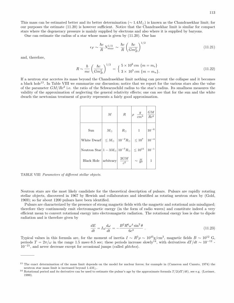
113
This mass can be estimated better and its better determination (∼ 1.4M¯) is known as the Chandrasekhar limit; forour purposes the estimate (11.20) is however sufficient. Notice that the Chandrasekhar limit is similar for compactstars where the degeneracy pressure is mainly supplied by electrons and also where it is supplied by baryons.
One can estimate the radius of a star whose mass is given by (11.20). One has
εF ∼ ~cR
N1/3max ∼ ~c
R
(~c
Gm2B
)1/2
(11.21)
and, therefore,
R ∼ ~mc
(~c
Gm2B
)1/2
= 5× 108 cm m = me
3× 105 cm m = mn.(11.22)
If a neutron star accretes its mass beyond the Chandrasekhar limit nothing can prevent the collapse and it becomesa black hole13. In Table VIII we summarize our discussion; notice that we report for the various stars also the valueof the parameter GM/Rc2 i.e. the ratio of the Schwarzschild radius to the star’s radius. Its smallness measures thevalidity of the approximation of neglecting the general relativity effects; one can see that for the sun and the whitedwarfs the newtonian treatment of gravity represents a fairly good approximation.
M R ρ g
cm3
GM
Rc2
Sun M¯ R¯ 1 10−6
White Dwarf ≤ M¯ 10−2R¯ ≤ 107 10−4
Neutron Star 1− 3M¯ 10−5R¯ ≤ 1015 10−1
Black Hole arbitrary2GM
c2∼ M
R3 1
TABLE VIII Parameters of different stellar objects.
Neutron stars are the most likely candidate for the theoretical description of pulsars. Pulsars are rapidly rotatingstellar objects, discovered in 1967 by Hewish and collaborators and identified as rotating neutron stars by (Gold,1969); so far about 1200 pulsars have been identified.
Pulsars are characterized by the presence of strong magnetic fields with the magnetic and rotational axis misaligned;therefore they continuously emit electromagnetic energy (in the form of radio waves) and constitute indeed a veryefficient mean to convert rotational energy into electromagnetic radiation. The rotational energy loss is due to dipoleradiation and is therefore given by
dE
dt= Iω
dω
dt= −B2R6ω4 sin2 θ
6c3. (11.23)
Typical values in this formula are, for the moment of inertia I ∼ R5ρ ∼ 1045g/cm3, magnetic fields B ∼ 1012 G,periods T = 2π/ω in the range 1.5 msec-8.5 sec; these periods increase slowly14, with derivatives dT/dt ∼ 10−12 -10−21, and never decrease except for occasional jumps (called glitches).
13 The exact determination of the mass limit depends on the model for nuclear forces; for example in (Cameron and Canuto, 1974) theneutron star mass limit is increased beyond 1.4M¯.
14 Rotational period and its derivative can be used to estimate the pulsar’s age by the approximate formula T/2(dT/dt), see e.g. (Lorimer,1999).

114
Glitches were first observed in the Crab and Vela pulsars in 1969; the variations in the rotational frequency are ofthe order 10−8 − 10−6.
This last feature is the most significant phenomenon pointing to neutron stars as a model of pulsars in comparisonto other form of hadronic matter, such as strange quarks. It will be discussed in more detail in Section XI.E, where wewill examine the possible role played by the crystalline superconducting phase. In the subsequent three paragraphswe will instead deal with other possible astrophysical implications of color superconductivity.
B. Supernovae neutrinos and cooling of neutron stars
Neutrino diffusion is the single most important mechanism in the cooling of young neutron stars, i.e. with an age< 105 years; it affects both the early stage and the late time evolution of these compact stars. To begin with let usconsider the early evolution of a Type II Supernova.
Type II supernovae are supposed to be born by collapse of massive (M ∼ 8 − 20M¯) stars15. These massivestars have unstable iron cores16 with masses of the order of the Chandrasekhar mass. The explosion producing thesupernova originates within the core, while the external mantle of the red giant star produces remnants that can beanalyzed by different means, optical, radio and X rays. These studies agree with the hypothesis of a core explosion.The emitted energy (∼ 1051erg) is much less than the total gravitational energy of the star, which confirms that theremnants are produced by the outer envelope of the massive star; the bulk of the gravitational energy, of the order of1053 erg, becomes internal energy of the proto neutron star (PNS). The suggestion that neutron stars may be formedin supernovae explosions was advanced in 1934 by (Baade and Zwicky, 1934) and it has been subsequently confirmedby the observation of the Crab pulsar in the remnant of the Crab supernova observed in China in 1054 A.D.
We do not proceed in this description as it is beyond the scope of this review and we concentrate our attention onthe cooling of the PNS17, which is mostly realized through neutrino diffusion. By this mechanism one passes from theinitial temperature T ∼ 20− 30 MeV to the cooler temperatures of the neutron star at subsequent stages. This phaseof fast cooling lasts 10-20 secs and the neutrinos emitted during it have mean energy ∼ 20 MeV. These properties,that can be predicted theoretically, are also confirmed by data from SN 1987A.
The role of quark color superconductivity at this stage of the evolution of the neutron stars has been discussedin (Carter and Reddy, 2000). In this paper the neutrino mean free path is computed in a color super-conductingmedium made up by quarks in two flavor (2SC model). The results obtained indicate that the cooling process byneutrino emission slows down when the quark matter undergoes the phase transition to the superconducting phaseat the critical temperature Tc, but then accelerates when T decreases below Tc. There should be therefore changes inthe neutrino emission by the PNS and they might be observed in some future supernova event; this would producean interesting test for the existence of a color superconducting phase in compact stars.
Let us now consider the subsequent evolution of the neutron star, which also depends on neutrino diffusion. Thesimplest processes of neutrino production are the so called direct Urca processes
f1 + ` → f2 + ν` ,
f2 + ` → f1 + ` → f2 + ν` ; (11.24)
by these reactions, in absence of quark superconductivity, the interior temperature T of the star drops below 109
K (∼ 100 KeV) in a few minutes and in 102 years to temperatures ∼ 107 K. Generally speaking the effect of theformation of gaps is to slow down the cooling, as it reduces both the emissivity and the specific heat. However notonly quarks, if present in the neutron star, but also other fermions, such as neutrons, protons or hyperons have gaps,as the formation of fermion pairs is unavoidable if there is an attractive interaction in any channel. Therefore, besidesquark color superconductivity, one has also the phenomenon of baryon superconductivity and neutron superfluidity,which is the form assumed by this phenomenon for neutral particles. The analysis is therefore rather complicated;the thermal evolution of a late time neutron star has been discussed in (Blaschke et al., 2000; Page et al., 2000),but no clear signature for the presence of color superconductivity seems to emerge from the theoretical simulationsand, therefore, one may tentatively conclude that the late time evolution of the neutron stars does not offer a goodlaboratory to test the existence of color superconductivity in compact stars.
15 The other supernovae, i.e. type I supernovae, result from the complete explosion of a star with 4M¯ ≤ M ≤ 8M¯ with no remnants.16 Fusion processes favor the formation of iron, as the binding energy per nucleon in nuclei has a maximum for A ∼ 60.17 See (Burrows and Lattimer, 1986; Colgate and White, 1966; Imsshennyk and Nadyozhin, 1973; Keil and Janka, 1995; Pons and et al,
1999) for further discussions.

115
C. R-mode instabilities in neutron stars and strange stars
Rotating relativistic stars are in general unstable against the rotational mode (r-mode instability) (Andersson,1998). The instability is due to the emission of angular momentum by gravitational waves from the mode. Unlessit is damped by viscosity effects, this instability would spin down the star in relatively short times. More recently ithas been realized (Andersson et al., 2000; Bildsten and Ushomirsky, 1999) that in neutron stars there is an importantviscous interaction damping the r-mode i.e. that between the external metallic crust and the neutron superfluid. Theconsequence of this damping is that r-modes are significant only for young neutron stars, with periods T < 2 msec.For larger rotating periods the damping of the r−mode implies that the stars slow down only due to magnetic dipolebraking.
All this discussion is relevant for the nature of pulsars: Are they neutron stars or strange stars?The existence of strange stars, i.e. compact stars made of quarks u, d, s in equal ratios would be a consequence
of the existence of stable strangelets. This hypothetical form of nuclear matter, made of a large number of u, d, squarks has been suggested by (Bodmer, 1971) and (Witten, 1984) as energetically favored in comparison to otherhadronic phases when a large baryonic number is involved. The reason is that in this way the fermions, being ofdifferent flavors, could circumvent the Pauli principle and have a lower energy, in spite of the larger strange quarkmass. If strangelets do exist, basically all the pulsars should be strange stars because the annihilation of strange stars,for example from a binary system, would fill the space around with strangelets that, in turn, would convert ordinarynuclear stars into strange stars.
An argument in favor of the identification of pulsars with strange stars is the scarcity of pulsars with very highfrequency (T < 2.5 msec).
This seems to indicate that indeed the r−mode instability is effective in slowing down the compact stars andfavors strange stars, where, differently from neutron stars, the crust can be absent. Even in the presence of theexternal crust, that in a quark star can be formed by the gas after the supernova explosion or subsequent accretion,the dampening of the r − mode is less efficient. As a matter of fact, since electrons are only slightly bounded, incomparison with quarks that are confined, they tend to form an atmosphere having a thickness of a few hundredFermi; this atmosphere produces a separation between the nuclear crust and the inner quark matter and thereforethe viscosity is much smaller.
In quark matter with color superconductivity the presence of gaps ∆ À T exponentially reduces the bulk and shearviscosity, which renders the r−mode unstable. According to (Madsen, 2000, 2002) this would rule out compact starsentirely made of quarks in the CFL case (the 2SC model would be marginally compatible, as there are ungappedquarks in this case). For example for ∆ > 1 MeV any star having T < 10 msec would be unstable, which wouldcontradict the observed existence of pulsars with time period less than 10 msec.
However this conclusion does not rule out the possibility of neutron stars with a quark core in the color super-conducting state, because as we have stressed already, for them the dampening of the r−mode instability would beprovided by the viscous interaction between the nuclear crust and the neutron superfluid.
D. Miscellaneous results
Color superconductivity is a Fermi surface phenomenon and as such, it does not affect significantly the equationof state of the compact star. Effects of this phase could be seen in other astrophysical contexts, such as thoseconsidered in the two previous paragraphs or in relation to the pulsar glitches, which will be examined in the nextparagraph. A few other investigations have been performed in the quest of possible astrophysical signatures of colorsuperconductivity; for instance in (Ouyed and Sannino, 2001) it has been suggested that the existence of a 2SC phasemight be partly responsible of the gamma ray bursts, due to the presence in the two-flavor superconducting phase of alight glueball that can decay into two photons. Another interesting possibility is related to the stability of strangelets,because, as observed in (Madsen, 2001), CFL strangelets, i.e. lumps of strange quark matter in the CFL phase maybe significantly more stable than strangelets without color superconductivity.
Finally we wish to mention the observation of (Alford et al., 2000) concerning the evolution of the magnetic fieldin the interior of neutron stars. Inside an ordinary neutron star, neutron pairs are responsible for superfluidity, whileproton pairs produce BCS superconductivity. In this condition magnetic fields experience the ordinary Meissner effectand are either expelled or restricted to flux tubes where there is no pairing. In the CFL (and also 2SC) case, as weknow from V.D, a particular U(1) group generated by
Q = 1⊗Q−Q⊗ 1 (11.25)
remains unbroken and plays the role of electromagnetism. Instead of being totally dragged out or confined in fluxtubes, the magnetic field will partly experience Meissner effect (the component Aµ), while the remaining part will
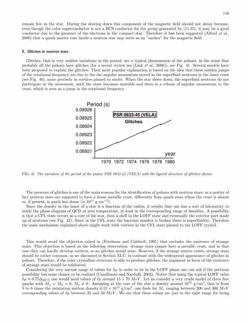
116
remain free in the star. During the slowing down this component of the magnetic field should not decay because,even though the color superconductor is not a BCS conductor for the group generated by (11.25), it may be a goodconductor due to the presence of the electrons in the compact star. Therefore it has been suggested (Alford et al.,2000) that a quark matter core inside a neutron star may serve as an ”anchor” for the magnetic field.
E. Glitches in neutron stars
Glitches, that is very sudden variations in the period, are a typical phenomenon of the pulsars, in the sense thatprobably all the pulsars have glitches (for a recent review see (Link et al., 2000)), see Fig. 41. Several models havebeen proposed to explain the glitches. Their most popular explanation is based on the idea that these sudden jumpsof the rotational frequency are due to the the angular momentum stored in the superfluid neutrons in the inner crust(see Fig. 40), more precisely in vortices pinned to nuclei. When the star slows down, the superfluid neutrons do notparticipate in the movement, until the state becomes unstable and there is a release of angular momentum to thecrust, which is seen as a jump in the rotational frequency.
PSR 0833-45 (VELA)
1970 1972 1974 1976 1978 1980
0.08921
0.08922
0.08923
0.08924
0.08925
0.08926
Glitches
Period (s)
year
FIG. 41 The variation of the period of the pulsar PSR 0833-45 (VELA) with the typical structure of glitches shown.
The presence of glitches is one of the main reasons for the identification of pulsars with neutron stars; as a matter offact neutron stars are supposed to have a dense metallic crust, differently from quark stars where the crust is absentor, if present, is much less dense (≈ 1011 g cm−3).
Since the density in the inner of a star is a function of the radius, it results that one has a sort of laboratory tostudy the phase diagram of QCD at zero temperature, at least in the corresponding range of densities. A possibilityis that a CFL state occurs as a core of the star, then a shell in the LOFF state and eventually the exterior part madeup of neutrons (see Fig. 42). Since in the CFL state the baryonic number is broken there is superfluidity. Thereforethe same mechanism explained above might work with vortices in the CFL state pinned to the LOFF crystal.
This would avoid the objection raised in (Friedman and Caldwell, 1991) that excludes the existence of strangestars. This objection is based on the following observation: strange stars cannot have a metallic crust, and in thatcase they can hardly develop vortices, so no glitches would arise. However, if the strange matter exists, strange starsshould be rather common, as we discussed in Section XI.C, in contrast with the widespread appearance of glitches inpulsars. Therefore, if the color crystalline structure is able to produce glitches, the argument in favor of the existenceof strange stars would be reinforced.
Considering the very narrow range of values for δµ in order to be in the LOFF phase one can ask if the previouspossibility has some chance to be realized (Casalbuoni and Nardulli, 2003). Notice that using the typical LOFF valueδµ ≈ 0.75∆BCS one would need values of δµ around 15÷ 70 MeV . Let us consider a very crude model of three freequarks with Mu = Md = 0, Ms 6= 0. Assuming at the core of the star a density around 1015 g/cm3, that is from5 to 6 times the saturation nuclear density 0.15 × 10¹⁵ g/cm3, one finds for Ms ranging between 200 and 300 MeVcorresponding values of δµ between 25 and 50 MeV . We see that these values are just in the right range for being

117
CFL
LOFF
Hadronic
FIG. 42 A model of a neutron star with an inner shell in the LOFF phase.
within the LOFF window. Therefore a possible phase diagram for QCD could be of the form illustrated in Fig. 43.We see that in this case a coexistence of the CFL, LOFF and neutron matter would be possible inside the neutronstar.
QGP
2SC
CFL
T
µ
tricr
m >> m = 0s u,d/
LOFF
neutron stars
hadrons
FIG. 43 A possible QCD phase diagram showing the end point of the first order transition phase, labelled as ”tricr”. The hadronphase with the transition to the nuclear phase, the Quark-gluon plasma, the CFL, the 2SC and the LOFF phase are also shown.
Acknowledgments
I would like to thank the CERN Theory Division, the DESY Theory Group and the Department of Physics of theUniversity of Barcellona for the kind hospitality offered during the preparation and the completion of these lecturenotes. I would like to thank also all my collaborators to the work I have done in this subject. In particular I wouldlike to thank G. Nardulli, R. Gatto, M. Mannarelli and M. Ruggieri.

118
APPENDIX A: The gap equation in the functional formalism from HDET
We will now derive the gap equation by using the functional formalism within the general formalism of SectionV.B. The method used is a trivial generalization of the one used in Section III.C. We start again from Eq. 5.64
LI = −G
4εabεcdVABCDψA
a ψBb ψC†
c ψD†d
(A1)
For simplicity we suppress the notation for fixed velocity. We will insert inside the functional integral the followingidentity
const =∫D(∆AB , ∆∗
AB)e− i
G
∫d4xF [∆AB ,∆∗
AB , ψA, ψA†](A2)
where
F =[∆AB − G
2VGHAB(ψGT CψH)
]WABCD
[∆∗
CD +G
2VCDEF (ψE†CψF∗)
](A3)
The quantity WABCD is defined in such a way that
WABCDVCDEF = δAEδBF , VABCDWCDEF = δAEδDF (A4)
Then we get
F =G
4VABCDψCT CψBψC†CψD∗ +
12∆∗
CDψCT CψD − 12∆ABψA†CψB∗
− 1g∆ABWABCD∆∗
CD (A5)
Normalizing at the free case (G = 0) we get
Z
Z0=
1Z0
∫D(ψ, ψ†)D(∆, ∆∗)eiS0[ψ, ψ†]
× e+i
∫d4x
[−∆ABWABCD∆∗
CD
G− 1
2∆AB(ψA†CψB∗) +
12∆∗
AB(ψAT CψB)]
(A6)
Going to the velocity formalism and introducing the Nambu-Gor’kov field we can write the fermionic part in theexponent inside the functional integral as
∫d4x
∫dv4π
χA†S−1ABχB (A7)
with
S−1AB =
(V · ` δAB −∆AB
−∆∗AB V · ` δAB
)(A8)
Using again the replica trick as in Section III.C we perform the functional integral over the Fermi fields obtaining
Z
Z0=
1Z0
[detS−1
]e− i
G
∫d4x∆ABWABCD∆∗
CD ≡ eiSeff (A9)
with
Seff = − i
2Tr[log S0S
−1]− i
G
∫d4x∆ABWABCD∆∗
CD (A10)
Differentiating with respect to ∆AB we get immediately the gap equation (5.83).

119
APPENDIX B: Some useful integrals
We list a few 2-D integrals which have been used in the text (Nardulli, 2002). Let us define
In =∫
dN `
(V · ` V · `−∆2 + iε)n+1=
i (−i)n+1πN2
n!Γ(n + 1− N
2 )∆2n+2−N
; (B1)
therefore, for N = 2− ε and denoting by γ the Euler-Mascheroni constant, we get
I0 = −2iπ
ε+ iπ ln π∆2 + iπγ ,
I1 = +iπ
∆2, I2 = − iπ
2∆4, I3 = +
iπ
3∆6. (B2)
Moreover defining
In, m =∫
d2`
(V · ` V · `−∆2 + iε)n(V · ` V · `−∆′2 + iε)m, (B3)
we find
I1, 1 =iπ
∆2 −∆′ 2 ln∆2
∆′ 2 ,
I2, 1 = iπ
[1
∆2(∆2 −∆′ 2)− 1
(∆2 −∆′ 2)2ln
∆2
∆′ 2
],
I3, 1 =iπ
2
[ −1∆4(∆2 −∆′ 2)
− 2∆2(∆2 −∆′ 2)2
+2
(∆2 −∆′ 2)3ln
∆2
∆′ 2
],
I2, 2 = iπ
[(1
∆2+
1∆′ 2
)1
(∆2 −∆′ 2)2+
2(∆2 −∆′ 2)3
ln∆2
∆′ 2
]. (B4)
Of some interest is the following infrared divergent integral:
I1 =∫
(V · `)2 d2`
(V · ` V · `)2 . (B5)
We can regularize the divergence by going to finite temperature and then taking the limit T → 0 (`0 = iωn, ωn =πT (2n + 1); T → 0, µ →∞):
I1 = 2πTi
∫ +µ
−µ
dx
+∞∑−∞
(iωn − x)2
(x2 + ω2n)2
= 2πT i
(− 1
Ttanh
µ
2T
)→ −2πi . (B6)
Other divergent integrals, such as
I =∫
d2`
(V · ` V · `)(V · ` V · `−∆2)(B7)
are treated in a similar way.Finally, useful angular integrations are:
∫dv4π
vjvk =δjk
3, (B8)
∫dv4π
vivjvkv` =115
(δijδk` + δikδj` + δi`δjk) . (B9)

120
References
Abbott, L. F., and E. Fahri, 1981, CERN-TH3015 .Abrikosov, A. A., 1957, Zh. Exsp. teor. Fiz. 32, 1442.Abrikosov, A. A., L. P. Gor’kov, and I. E. Dzyaloshinski, 1963, Methods of Quantum Field Theory in Statistical Physics (Dover,
New York).Alford, M. G., 2001, Ann. Rev. Nucl. Part. Sci. 51, 131.Alford, M. G., J. Berges, and K. Rajagopal, 2000, Nucl. Phys. B571, 269.Alford, M. G., J. A. Bowers, J. M. Cheyne, and G. A. Cowan, 2003, Phys. Rev. D67, 054018.Alford, M. G., J. A. Bowers, and K. Rajagopal, 2001, Phys. Rev. D63, 074016.Alford, M. G., K. Rajagopal, and F. Wilczek, 1998, Phys. Lett. B422, 247.Alford, M. G., K. Rajagopal, and F. Wilczek, 1999, Nucl. Phys. B537, 443.Andersson, N., 1998, Astrophys. J. 502, 708.Andersson, N., D. I. Jones, K. D. Kokkotas, and N. Stergioulas, 2000, Astrophys. J. 534, L75.Baade, W., and F. Zwicky, 1934, Proc. Nat. Acad. Sci. 20.Bailin, D., and A. Love, 1984, Phys. Rept. 107, 325.Banks, T., and E. Rabinovici, 1979, Nucl. Phys. B160, 349.Bardeen, J., 1956, in Handbuch der Physik. vol XV (Springer Verlag, Berlin).Bardeen, J., L. N. Cooper, and J. R. Schrieffer, 1957, Phys. Rev. 106, 162.Barrois, B. C., 1977, Nucl. Phys. B129, 390.Beane, S. R., P. F. Bedaque, and M. J. Savage, 2000, Phys. Lett. B483, 131.Bedaque, P. F., and T. Schafer, 2002, Nucl. Phys. A697, 802.Benfatto, G., and G. Gallavotti, 1990, Phys. Rev. B42, 9967.Bildsten, L., and G. Ushomirsky, 1999, eprint astro-ph/9911155.Blaschke, D., T. Klahn, and D. N. Voskresensky, 2000, Astrophys. J. 533, 406.Bodmer, A. R., 1971, Phys. Rev. D4, 1601.Bowers, J. A., 2003, eprint hep-ph/0305301.Bowers, J. A., and K. Rajagopal, 2002, Phys. Rev. D66, 065002.Brown, W. E., J. T. Liu, and H.-c. Ren, 2000a, Phys. Rev. D62, 054013.Brown, W. E., J. T. Liu, and H.-c. Ren, 2000b, Phys. Rev. D61, 114012.Brown, W. E., J. T. Liu, and H.-c. Ren, 2000c, Phys. Rev. D62, 054016.Buckley, K. B. W., and A. R. Zhitnitsky, 2002, JHEP 08, 013.Burrows, A., and J. M. Lattimer, 1986, Astrophys. J. 307.Buzdin, A. I., and Kachkachi, 1997, Phys. Lett. A225, 341.Cameron, A. G. W., and V. Canuto, 1974, in Proceedings 16th Solvay Conference on Astrophysics and Gravitation (Universite
Libre de Bruxelles).Carter, G. W., and S. Reddy, 2000, Phys. Rev. D62, 103002.Casalbuoni, R., F. De Fazio, R. Gatto, G. Nardulli, and M. Ruggieri, 2002a, Phys. Lett. B547, 229.Casalbuoni, R., Z.-y. Duan, and F. Sannino, 2000, Phys. Rev. D62, 094004.Casalbuoni, R., Z.-y. Duan, and F. Sannino, 2001a, Phys. Rev. D63, 114026.Casalbuoni, R., E. Fabiano, R. Gatto, M. Mannarelli, and G. Nardulli, 2002b, Phys. Rev. D66, 094006.Casalbuoni, R., and R. Gatto, 1981, Phys. Lett. B103, 113.Casalbuoni, R., and R. Gatto, 1999, Phys. Lett. B464, 111.Casalbuoni, R., R. Gatto, M. Mannarelli, and G. Nardulli, 2001b, Phys. Lett. B511, 218.Casalbuoni, R., R. Gatto, M. Mannarelli, and G. Nardulli, 2002c, Phys. Rev. D66, 014006.Casalbuoni, R., R. Gatto, M. Mannarelli, and G. Nardulli, 2002d, Phys. Lett. B524, 144.Casalbuoni, R., R. Gatto, and G. Nardulli, 2001c, Phys. Lett. B498, 179.Casalbuoni, R., R. Gatto, and G. Nardulli, 2001d, Phys. Lett. (B498 Erratum) B517, 483.Casalbuoni, R., R. Gatto, and G. Nardulli, 2002e, Phys. Lett. B543, 139.Casalbuoni, R., R. Gatto, G. Nardulli, and M. Ruggieri, 2003, eprint hep-ph/0302077.Casalbuoni, R., and G. Nardulli, 2003, eprint hep-ph/0305069.Chandrasekhar, B. S., 1962, App. Phys. Lett. 1, 7.Cini, M., and B. Touschek, 1958, Nuovo Cimento 7, 422.Clogston, A. M., 1962, Phys. Rev. Lett. 9, 266.Colgate, S. A., and R. H. White, 1966, Astrophys. J. 143.Collins, J. C., and M. J. Perry, 1975, Phys. Rev. Lett. 34, 1353.Combescot, R., and C. Mora, 2002, Eur. P. J. B28, 397.Cooper, L. N., 1956, Phys. Rev. 104, 1189.Corak, W. S., B. B. Goodman, C. B. Satterthwaite, and A. Wexler, 1954, Phys. Rev. 96, 1442.Corak, W. S., B. B. Goodman, C. B. Satterthwaite, and A. Wexler, 1956, Phys. Rev. 102, 656.Daunt, J. G., and K. Mendelssohn, 1946, Proc. Roy. Soc. A185, 225.Dimopoulos, S., S. Raby, and L. Susskind, 1980a, Nucl. Phys. B169, 373.Dimopoulos, S., S. Raby, and L. Susskind, 1980b, Nucl. Phys. B173, 208.

121
Eguchi, T., 1976, Phys. Rev. D14, 2755.Eliashberg, G. M., 1960, Sov. Phys. JETP 11, 696.Evans, N., J. Hormuzdiar, S. D. H. Hsu, and M. Schwetz, 2000, Nucl. Phys. B581, 391.Evans, N., S. D. H. Hsu, and M. Schwetz, 1999a, Nucl. Phys. B551, 275.Evans, N., S. D. H. Hsu, and M. Schwetz, 1999b, Phys. Lett. B449, 281.Fradkin, E., and S. H. Shenker, 1979, Phys. Rev. D19, 3682.Frautschi, S. C., 1978, presented at Workshop on Hadronic Matter at Extreme Energy Density, Erice, Italy, Oct 13-21, 1978.Friedman, J. L., and R. R. Caldwell, 1991, Phys. Lett. B264, 143.Frolich, H., 1950, Phys. Rev. 79, 845.Frolich, H., 1952, Proc. Roy. Soc. A215, 291.Fulde, P., and R. A. Ferrell, 1964, Phys. Rev. 135, A550.de Gennes, P. G., 1989, Superconductivity in Metals and Alloys (Addison Wesley, Reading, MA).Ginzburg, L., and L. D. Landau, 1950, Zh. Exsp. teor. Fiz. 20, 1064.Ginzburg, V. L., 1953, Fortschr. Phys. 1, 101.Ginzburg, V. L., and E. A. Andryushin, 1994, Superconductivity (World Scientific).Glover, R. E., and M. Tinkham, 1956, Phys. Rev. 104, 844.Gold, T., 1969, Nature 221, 25.Gor’kov, L. P., 1959, Zh. Exsp. teor. Fiz. 36, 1918.Gorter, C. J., and H. G. B. Casimir, 1934a, Phys. Z. 35, 963.Gorter, C. J., and H. G. B. Casimir, 1934b, Z. Tech. Phys. 15, 539.Gross, D., and F. Wilczek, 1973, Phys. Rev. Lett. 30, 1343.Gusynin, V. P., and I. A. Shovkovy, 2002, Nucl. Phys. A700, 577.Heiselberg, H., and V. Pandharipande, 2000, Ann. Rev. Nucl. Part. Sci. 50, 481.Hong, D. K., 2000a, Nucl. Phys. B582, 451.Hong, D. K., 2000b, Phys. Lett. B473, 118.Hong, D. K., 2001, Acta Phys. Polon. B32, 1253.Hong, D. K., T. Lee, and D.-P. Min, 2000a, Phys. Lett. B477, 137.Hong, D. K., V. A. Miransky, I. A. Shovkovy, and L. C. R. Wijewardhana, 2000b, Phys. Rev. D61, 056001.Hong, D. K., M. Rho, and I. Zahed, 1999, Phys. Lett. B468, 261.’t Hooft, G., 1976, Phys. Rev. Lett. 37, 8.’t Hooft, G., 1980, in Recent Developments in Gauge Theories (Plenum Press).Hsu, S. D. H., 2000, eprint hep-ph/0003140.Hsu, S. D. H., F. Sannino, and M. Schwetz, 2001, Mod. Phys. Lett. A16, 1871.Imsshennyk, V. S., and D. K. Nadyozhin, 1973, Sov. Phys. JETP 36.Jackson, A. D., and F. Sannino, 2003, eprint hep-ph/0308182.Jaffe, R. L., 1977, Phys. Rev. Lett. 38, 195, 617(E).Jaikumar, P., M. Prakash, and T. Schafer, 2002, Phys. Rev. D66, 063003.Josephson, D., 1962, Phys. Lett. 1, 251.Josephson, D., 1965, Adv. Phys. 14, 419.Kamerlingh Onnes, H., 1911, Leiden Comm. 120b, 122b, 124c.Kaplan, D. B., and S. Reddy, 2002a, Phys. Rev. D65, 054042.Kaplan, D. B., and S. Reddy, 2002b, Phys. Rev. Lett. 88, 132302.Keil, W., and H. T. Janka, 1995, Astron. Astrophys. 296.Kundu, J., and K. Rajagopal, 2002, Phys. Rev. D65, 094022.Landau, L., and E. M. Lifshitz, 1996, Statistical Physics, Part I (Butterworth, Heinemann).Landau, L., E. M. Lifshitz, and L. P. Pitaevskii, 1980, Statistical Physics, Part II (Oxford: Pergamon).Larkin, A. J., and Y. N. Ovchinnikov, 1964, Zh. Exsp. teor. Fiz. 47, 1136.Le Bellac, M., 1996, Thermal Field Theory (Cambridge University Press, Cambridge, England).Leibovich, A. K., K. Rajagopal, and E. Shuster, 2001, Phys. Rev. D64, 094005.Link, B., R. I. Epstein, and J. M. Lattimer, 2000, eprint astro-ph/0001245.London, F., and H. London, 1935, Proc. Roy. Soc. A149, 71.Lorimer, D. R., 1999, eprint astro-ph/9911519.Madsen, J., 2000, Phys. Rev. Lett. 85, 10.Madsen, J., 2001, Phys. Rev. Lett. 87, 172003.Madsen, J., 2002, eConf C010815, 155.Manuel, C., and M. H. G. Tytgat, 2000, Phys. Lett. B479, 190.Manuel, C., and M. H. G. Tytgat, 2001, Phys. Lett. B501, 200.Maxwell, E., 1950, Phys. Rev. 78, 477.Meissner, W., and R. Ochsenfeld, 1933, Naturwissenschaften 21, 787.Miransky, V. A., and I. A. Shovkovy, 2002, Phys. Rev. Lett. 88, 111601.Nambu, Y., 1960, Phys. Rev. 117, 648.Nambu, Y., and G. Jona-Lasinio, 1961a, Phys. Rev. 122, 345.Nambu, Y., and G. Jona-Lasinio, 1961b, Phys. Rev. 124, 246.Nardulli, G., 2002, Riv. Nuovo Cim. 25N3, 1.

122
Nielsen, H. B., and S. Chada, 1976, Nucl. Phys. B105, 445.Ouyed, R., and F. Sannino, 2001, Phys. Lett. B511, 66.Page, D., 1998, in The Many Faces of Neutron Stars (Kluwer Academic Publishers).Page, D., M. Prakash, J. M. Lattimer, and A. Steiner, 2000, Phys. Rev. Lett. 85, 2048.Pines, D., 1958, Phys. Rev. 109, 280.Pippard, A. B., 1953, Proc. Roy. Soc. A216, 547.Pisarski, R. D., and D. H. Rischke, 1999, Phys. Rev. D60, 094013.Pisarski, R. D., and D. H. Rischke, 2000a, Phys. Rev. D61, 074017.Pisarski, R. D., and D. H. Rischke, 2000b, Phys. Rev. D61, 051501.Polchinski, J., 1993, in Recent directions in particle theory: from superstrings and black holes to the standard model (TASI -
92) (World Scientific), eprint hep-th/9210046.Politzer, H. D., 1973, Phys. Rev. Lett. 30, 1346.Pons, J., and et al, 1999, Astrophys. J. 513.Rajagopal, K., and E. Shuster, 2000, Phys. Rev. D62, 085007.Rajagopal, K., and F. Wilczek, 2001, in At the frontier of particle physics, vol. 3 (World Scientific), eprint hep-ph/0011333.Rapp, R., T. Schafer, E. V. Shuryak, and M. Velkovsky, 1998, Phys. Rev. Lett. 81, 53.Rapp, R., T. Schafer, E. V. Shuryak, and M. Velkovsky, 2000, Annals Phys. 280, 35.Reddy, S., M. Sadzikowski, and M. Tachibana, 2003, Nucl. Phys. A714, 337.Reynolds, C. A., B. Serin, W. H. Wright, and L. B. Nesbitt, 1950, Phys. Rev. 78, 487.Rho, M., E. V. Shuryak, A. Wirzba, and I. Zahed, 2000a, Nucl. Phys. A676, 273.Rho, M., A. Wirzba, and I. Zahed, 2000b, Phys. Lett. B473, 126.Rischke, D. H., 2000, Phys. Rev. D62, 034007.Rischke, D. H., D. T. Son, and M. A. Stephanov, 2001, Phys. Rev. Lett. 87, 062001.Sakita, B., 1985, Quantum theory of many-variable systems and fields (World Scientific).Sannino, F., 2000, Phys. Lett. B480, 280.Sarma, G., 1963, J. Phys. Chem. Solids 24, 1029.Schafer, T., 2000a, Phys. Rev. Lett. 85, 5531.Schafer, T., 2000b, Nucl. Phys. B575, 269.Schafer, T., 2000c, Phys. Rev. D62, 094007.Schafer, T., 2002, Phys. Rev. D65, 074006.Schafer, T., 2003, eprint hep-ph/0304281.Schafer, T., and E. V. Shuryak, 1998, Rev. Mod. Phys. 70, 323.Schafer, T., D. T. Son, M. A. Stephanov, D. Toublan, and J. J. M. Verbaarschot, 2001, Phys. Lett. B522, 67.Schafer, T., and F. Wilczek, 1999a, Phys. Rev. Lett. 82, 3956.Schafer, T., and F. Wilczek, 1999b, Phys. Lett. B450, 325.Schafer, T., and F. Wilczek, 1999c, Phys. Rev. D60, 074014.Schafer, T., and F. Wilczek, 1999d, Phys. Rev. D60, 114033.Schrieffer, J. R., 1964, Theory of Superconductivity (The Benjamin/Cummings Publishing Company, Inc.).Shankar, R., 1994, Rev. Mod. Phys. 66, 129.Shapiro, S. L., and S. A. Teukolski, 1983, Black holes, White Dwarfs and Neutron Stars: The Physics of Compact Objects
(Wiley-Interscience).Shifman, M. A., A. I. Vainshtein, and V. I. Zakharov, 1980, Nucl. Phys. B163, 46.Shimahara, H., 1998, J. Phys. Soc. Japan 67, 736.Shovkovy, I. A., and P. J. Ellis, 2002, Phys. Rev. C66, 015802.Shovkovy, I. A., and L. C. R. Wijewardhana, 1999, Phys. Lett. B470, 189.Son, D. T., 1999, Phys. Rev. D59, 094019.Son, D. T., and M. A. Stephanov, 2000a, Phys. Rev. D61, 074012.Son, D. T., and M. A. Stephanov, 2000b, Phys. Rev. (D61 Erratum) D62, 059902.Son, D. T., M. A. Stephanov, and A. R. Zhitnitsky, 2001, Phys. Rev. Lett. 86, 3955.Tinkham, M., 1995, Introduction to Superconductivity (McGraw-Hill).Tsuruta, S., 1998, Phys. Rep. 292, 1.Wang, Q., and D. H. Rischke, 2002, Phys. Rev. D65, 054005.Weinberg, S., 1996, The Quantum theory of Fields, Vol. II (Cambridge University Press).Witten, E., 1984, Phys. Rev. D30, 272.Zarembo, K., 2000, Phys. Rev. D62, 054003.Ziman, J. M., 1964, Principles of the Theory of Solids (Cambridge University Press, New York).