LECTURE NOTES

ON

INFORMATION RETRIEVAL SYSTEMS

IVB.TECH I SEMESTER (JNTUA-R13)

Mr.N.Parashuram Assistant Professor

Dr. S. Prem Kumar

Head of the Department

DEPARTMENT OF COMPUTER SCIENCE AND ENGINEERING

G.PULLAIAH COLLEGE OF ENGINEERING AND TECHNOLOGY

KURNOOL

G.PULLAIAH COLLEGE OF ENGINEERING AND TECHNOLOGY,KURNOOL DEPARTMENT OF COMPUTER SCIENCE AND ENGINEERING

IV B.TECH I SEM (R13)

INFORMATION RETRIEVAL SYSTEMS

UNIT-1

UNIT -1

Retrieval Strategies

INTRODUCTION:

Information Retrival System is a system it is a capable of stroring, maintaining from a system. and retrieving of information. This information May Any of the form that is audio,vedio,text.

Information Retrival System is mainly focus electronic searching and retrieving of documents.

Information Retrival is a activity of obtaining relevant documents based on user needs from collection of retrieved documents.

Fig shows basic information retrieval system

A static, or relatively static, document collection is indexed prior to any user query.

A query is issued and a set of documents that are deemed relevant to the query are ranked based on their computed similarity to the query and presented to the user query.

Information Retrieval (IR) is devoted to finding relevant documents, not finding simple matches to patterns.

A related problem is that of document routing or filtering. Here, the queries are static and the document collection constantly changes. An environment where corporate e-mail is routed based on predefined queries to different parts of the organization (i.e., e-mail about sales is routed to the sales department,marketing e-mail goes to marketing, etc.) is an example of an application of document routing. Figure illustrates document routing

Fig: Document routing algorithms

PRECISION AND RECALL:

In Figure we illustrate the critical document categories that correspond to any issued query.

Namely, in the collection there are documents which are retrieved, and there are those documents

that are relevant. In a perfect system, these two sets would be equivalent; we would only retrieve

relevant documents. In reality, systems retrieve many non-relevant documents. To measure

effectiveness, two ratios are used: precision and recall. Precision is the ratio of the number of

relevant documents retrieved to the total number retrieved. Precision provides an indication of

the quality of the answer set. However, this does not consider the total number of relevant

documents. A system might have good precision by retrieving ten documents and finding that

nine are relevant(a 0.9 precision), but the total number of relevant documents also matters. If

there were only nine relevant documents, the system would be a huge success.however if

millions of documents were relevant and desired, this would not be a good result set. Recall considers the total number of relevant documents; it is the ratio of the number of relevant

documents retrieved to the total number of documents in the collection that are believed to be relevant. Computing the total number of relevant documents is non-trivial.

Fig: PRECISION AND RECALL

1. RETRIEVAL STRATEGIES:

Retrieval strategies assign a measure of similarity between a query and a document. These

strategies are based on the common notion that the more often terms are found in both the

document and the query, the more "relevant" the document is deemed to be to the query. Some of

these strategies employ counter measures to alleviate problems that occur due to the ambiguities

inherent in language-the reality that the same concept can often be described withmany different

terms. A retrieval strategy is an algorithm that takes a query Q and a set of documents D1 , D2 , ... , Dn and identifies the Similarity Coefficient SC(Q,Di) for each of the documents 1 :s: i :s: n

The retrieval strategies identified are:

1.1 Vector Space Model

Both the query and each document are represented as vectors in the term space. A measure of the

similarity between the two vectors is computed. The vector space model computes a measure of

similarity by defining a vector that represents each document, and a vector that represents the

query The model is based on the idea that, in some rough sense, the meaning of a document is

conveyed by the words used. If one can represent the words in the document by a vector, it is

possible to compare documents with queries to determine how similar their content is. If a query

is considered to be like a document, a similarity coefficient (SC) that measures the similarity

between a document and a query can be computed. Documents whose content, as measured by

the terms in the document, correspond most closely to the content of the query are judged to be

the most relevant.

Figure illustrates the basic notion of the vector space model in which vectors that represent a query and three documents are illustrated.

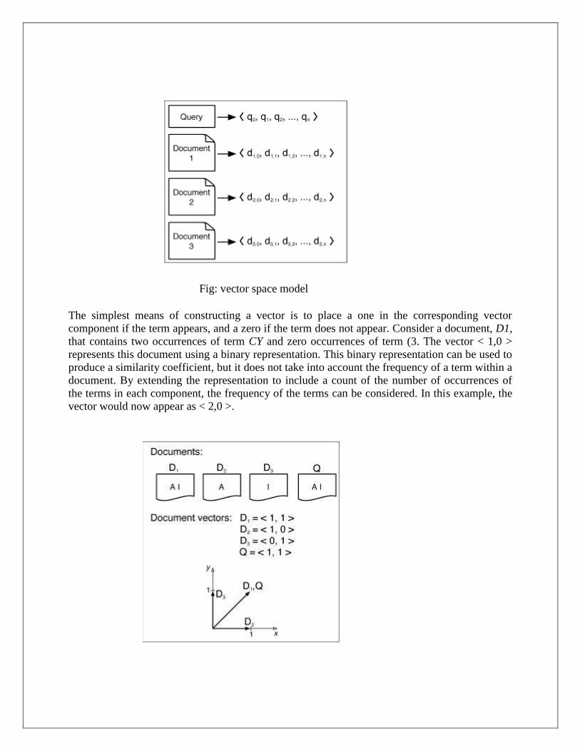
Fig: vector space model

The simplest means of constructing a vector is to place a one in the corresponding vector

component if the term appears, and a zero if the term does not appear. Consider a document, D1,

that contains two occurrences of term CY and zero occurrences of term (3. The vector < 1,0 >

represents this document using a binary representation. This binary representation can be used to

produce a similarity coefficient, but it does not take into account the frequency of a term within a

document. By extending the representation to include a count of the number of occurrences of

the terms in each component, the frequency of the terms can be considered. In this example, the

vector would now appear as < 2,0 >.

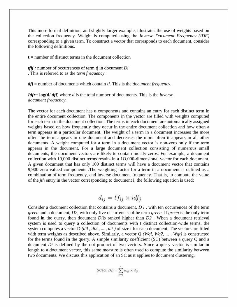
This more formal definition, and slightly larger example, illustrates the use of weights based on the collection frequency. Weight is computed using the Inverse Document Frequency (IDF)

corresponding to a given term. To construct a vector that corresponds to each document, consider the following definitions.

t = number of distinct terms in the document collection

tfij : number of occurrences of term tj in document Di . This is referred to as the term frequency.

dfj = number of documents which contain tj. This is the document frequency.

Idfr= log(d/ dfj) where d is the total number of documents. This is the inverse document frequency.

The vector for each document has n components and contains an entry for each distinct term in

the entire document collection. The components in the vector are filled with weights computed

for each term in the document collection. The terms in each document are automatically assigned

weights based on how frequently they occur in the entire document collection and how often a

term appears in a particular document. The weight of a term in a document increases the more

often the term appears in one document and decreases the more often it appears in all other

documents. A weight computed for a term in a document vector is non-zero only if the term

appears in the document. For a large document collection consisting of numerous small

documents, the document vectors are likely to contain mostly zeros. For example, a document

collection with 10,000 distinct terms results in a 1O,000-dimensional vector for each document.

A given document that has only 100 distinct terms will have a document vector that contains

9,900 zero-valued components .The weighting factor for a term in a document is defined as a

combination of term frequency, and inverse document frequency. That is, to compute the value

of the jth entry in the vector corresponding to document i, the following equation is used:

Consider a document collection that contains a document, D l , with ten occurrences of the term

green and a document, D2, with only five occurrences ofthe term green. If green is the only term

found in the query, then document Dlis ranked higher than D2 . When a document retrieval

system is used to query a collection of documents with t distinct collection-wide terms, the

system computes a vector D (dil , di2 , ... , dit ) of size t for each document. The vectors are filled

with term weights as described above. Similarly, a vector Q (Wql, Wq2, ... , Wqt) is constructed

for the terms found in the query. A simple similarity coefficient (SC) between a query Q and a

document Di is defined by the dot product of two vectors. Since a query vector is similar in

length to a document vector, this same measure is often used to compute the similarity between

two documents. We discuss this application of an SC as it applies to document clustering.

Example of Similarity Coefficient

Consider a case insensitive query and document collection with a query Q and a document collection consisting of the following three documents:

Q: "gold silver truck"

D l : "Shipment of gold damaged in a fire"

D2 : "Delivery of silver arrived in a silver truck"

D3: "Shipment of gold arrived in a truck"

In this collection, there are three documents, so d = 3. If a term appears in only one of the three

documents, its idfis log d~j = logf = 0.477. Similarly, if a term appears in two of the three

documents its idfis log ~ = 0.176, and a term which appears in all three documents has an idf of

log ~ = o.The idf for the terms in the three documents is given below: idfa = 0 idfarrived = 0.176 idfdamaged =

0.477 idfdelivery = 0.477 idfJire =

0.477 idfin = 0 idfof = 0

idfsilver = 0.477 idfshipment = 0.176 idftruck = 0.176 idfgold = 0.176

Document vectors can now be constructed. Since eleven terms appear in the document

collection, an eleven-dimensional document vector is constructed. The alphabetical ordering given above is used to construct the document vector so that h corresponds to term number

one which is a and t2 is arrived, etc. The weight for term i in vector j is computed as the idfi x t fij. The document

Similarly,

SC(Q, D2 ) = (0.954)(0.477) + (0.176)2 R:i 0.486

SC(Q, D3 ) = (0.176)2 + (0.176)2 R:i 0.062

Hence, the ranking would be D2 , D3 , D1 .

Implementations of the vector space model and other retrieval strategies typically use an inverted index to avoid a lengthy sequential scan through every document to find the terms in the query.

Instead, an inverted index is generated prior to the user issuing any queries. Figure illustrates the

structure of the inverted index. An entry for each of the n terms is stored in a structure called the

index. For each term, a pointer references a logical linked list called the posting list. The posting

list contains an entry for each unique document that contains the term. In the figure below, the

posting list contains both a document identifier and the term frequency. The posting list in the

figure indicates that term tl appears once in document one and twice in document ten. An entry

for an arbitrary term ti indicates that it occurs t f times in document j. Details of inverted index

construction and use are provided in Chapter 5, but it is useful to know that inverted indexes are

commonly used to improve run-time performance of various retrieval strategies.

Fig: inverted index

The measure is important as it is used by a retrieval system to identify which documents aredisplayed to the user. Typically, the user requests the top n documents, and these are

displayed ranked according to the similarity coefficient. Subsequently, work on term weighting was done to improve on the basic combination of tf-idf weights . Many variations were studied,

and the following weight for term j in document i was identifiedas a good performer:

The motivation for this weight is that a single matching term with a high term frequency can

skew the effect of remaining matches between a query and a given document. To avoid this, the

log(tf) + 1 is used reduce the range of term frequencies. A variation on the basic theme is to use

weight terms in the query differently than terms in the document. One term weighting scheme,

referred to as Inc. ltc, was effective. It uses a document weight of (1 + log(tf)) (idf) and query

weight of (1 + log(tf)). The labellnc.ltc is of the form: qqq.ddd where qqq refers to query weights

and ddd refers to document weights. The three letters: qqq or ddd are of the form xyz. The first

letter, x, is either n, l, or a. n indicates the "natural" term frequency or just t f is used. l indicates

that the logarithm is used to scale down the weight so 1 + log(tf) is used. a indicates that an

augmented weight was used where the weight is 0.5 + 0.5 x t/f . The second letter, y, indi2;tes

whether or not the idf was used. A value of n indicates that no idf was used while a value of t

indicates that the idf was used. The third letter, z, indicates whether or not document length

normalization was used. By normalizing for document length, we are trying to reduce the impact

document length might have on retrieval (see Equation 2.1). A value of n indicates no normalization was used, a value of c indicates the standard cosine normalization was used, and a value of u indicates pivoted length normalization.

1.2.Probabilistic Retrieval Strategies:

The probabilistic model computes the similarity coefficient (SC) between a query and a document as the probability that the document will be relevant to the query. This reduces the

relevance ranking problem to an application of probability theory. Probability theory can be used

to compute a measure of relevance between a query and a document.

1. Simple Term Weights.

2. Non binary independent model.

3. Language model.

1.2.1. Simple Term Weights:

The use of term weights is based on the Probability Ranking Principle (PRP),which assumes that optimal effectiveness occurs when documents are ranked based on an estimate of the probability

of their relevance to a query The key is to assign probabilities to components of the query and

then use each of these as evidence in computing the final probability that a document is relevant to the

query. The terms in the query are assigned weights which correspond to the probability that a

particular term, in a match with a given query, will retrieve a relevant document. The weights for

each term in the query are combined to obtain a final measure of relevance. Most of the papers in

this area incorporate probability theory and describe the validity of independence assumptions,

so a brief review of probability theory is in order. Suppose we are trying to predict whether or

not a softball team called the Salamanders will win one of its games. We might observe, based

on past experience, that they usually win on sunny days when their best shortstop plays. This

means that two pieces of evidence, outdoor-conditions and presence of good-shortstop, might be

used. For any given game, there is a seventy five percent chance that the team will win if the

weather is sunny and a sixty percent chance that the team will win if the shortstop plays.

Therefore, we write: P(win I sunny) = 0.75 P(win I good-shortstop) = 0.6

The conditional probability that the team will win given both situations is writtenas p(win I

sunny, good-shortstop). This is read "the probability that theteam will win given that there is a

sunny day and the good-shortstop plays."We have two pieces of evidence indicating that the

Salamanders will win. Intuition says that together the two pieces should be stronger than either

alone.This method of combining them is to "look at the odds." A seventy-five percent chance of

winning is a twenty-five percent chance of losing, and a sixty percent chance of winning is a

forty percent chance of losing. Let us assumethe independence of the pieces of evidence. P(win I sunny, good-shortstop) = a P( win I sunny) = (3 P(win I good-shortstop) = r

By Bayes' Theorem:

There fore,

Note the combined effect of both sunny weather and the good-shortstop results in a higher

probability of success than either individual condition. The key is the independence assumptions.

The likelihood of the weather being nice and the good-shortstop showing up are completely

independent. The chance the shortstop will show up is not changed by the weather. Similarly, he

weather is not affected by the presence or absence of the good-shortstop. If the independence

assumptions are violated suppose the shortstop prefer sunny weather - special consideration for

the dependencies is required. The independence assumptions also require that the weather and

the appearance of the good-shortstop are independent given either a win or a loss .For an

information retrieval query, the terms in the query can be viewed as indicators that a given

document is relevant. The presence or absence of query term A can be used to predict whether or

not a document is relevant. Hence, after a period of observation, it is found that when term A is

in both the query and the document, there is an x percent chance the document is relevant. We

then assign a probability to term A. Assuming independence of terms this can be done for each

of the terms in the query. Ultimately, the product of all the weights can be used to compute the

probability of relevance. We know that independence assumptions are really not a good model of reality. Some research has investigated why systems with these assumptions For example, a

relevant document that has the term apple in response to a query for apple pie probably has a better chance of having the term pie than some other randomly selected term. Hence, the key

independence assumption is violated.

Most work in the probabilistic model assumes independence of terms because handle

independencies involves substantial computation. It is unclear whether or not effectiveness is

improved when dependencies are considered. We note that relatively little work has been done

implementing these approaches. They are computationally expensive, but more importantly, they

are difficult to estimate. It is necessary to obtain sufficient training data about term co occurrence

in both relevant and non-relevant documents. Typically, it is very difficult to obtain sufficient

training data to estimate these parameters. In the need for training data with most probabilistic

models A query with two terms, ql and q2, is executed. Five documents are returned and an

assessment is made that documents two and four are relevant. From this assessment, the

probability that a document is relevant (or non-relevant) given that it contains term ql is

computed. Likewise, the same probabilities are computed for term q2. Clearly, these

probabilities are estimates based on training data. The idea is that sufficient training data can be

obtained so that when a user issues a query, a good estimate of which documents are relevant to

the query can be obtained. Consider a document, di, consisting of t terms (WI, W2, ... , Wt),

where Wi is the estimate that term i will result in this document being relevant. The weight or

"odds" that document di is relevant is based on the probability of relevance for each term in the

document. For a given term in a document, its contribution to the estimate of relevance for the

entire document is computed as

The question is then: How do we combine the odds of relevance for each term into an estimate for the entire document? Given our independence assumptions, we can multiply the odds for

each term in a document to obtain the odd is that the document is relevant. Taking the log of the product yields:

We note that these values are computed based on the assumption that terms will occur independently in relevant and non-relevant documents. The assumption is also made that if one

term appears in a document, then it has no impact on whether or not another term will appear in

the same document.

Now that we have described how the individual term estimates can be combined into a total

estimate of relevance for the document, it is necessary to describe a means of estimating the individual term weights. Several different means of computing the probability of relevance and

non-relevance for a given term were studied since the introduction of the probabilistic retrieval

model.

exclusive independence assumptions:

11: The distribution of terms in relevant documents is independent and their distribution in all documents is independent.

12: The distribution of terms in relevant documents is independent and their distribution in non-relevant documents is independent.

01: Probable relevance is based only on the presence of search terms in the documents.

02: Probable relevance is based on both the presence of search terms in documents and their absence from documents.

11 indicates that terms occur randomly within a document-that is, the presence of one term in a

document in no way impacts the presence of another term in the same document. This is

analogous to our example in which the presence of the good-shortstop had no impact on the

weather given a win. This also states that the distribution of terms across all documents is

independent un conditionally for all documents-that is, the presence of one term in a document

tin no way impacts the presence of the same term in other documents. This is analogous to

saying that the presence of a good-shortstop in one game has no impact on whether or not a

good-shortstop will play in any other game. Similarly, the presence of good-shortstop in one game has no impact on the weather for any other game.

12 indicates that terms in relevant documents are independent-that is, they satisfy 11 and terms in

non-relevant documents also satisfy 11. Returning to our example, this is analogous to saying

that the independence of a good-shortstop and sunny weather holds regardless of whether the

team wins or loses.01 indicates that documents should be highly ranked only if they contain

matching terms in the query (i.e., the only evidence used is which query terms are actually

present in the document). We note that this ordering assumption is not commonly held today

because it is also important to consider when query terms are not found in the document. This is

inconvenient in practice. Most systems use an inverted index that identifies for each term, all

occurrences of that term in a given document. If absence from a document is required, the index

would have to identify all terms not in a document To avoid the need to track the absence of a

term in a document, the estimate makes the zero point correspond to the probability of relevance

of a document lacking all the query terms-as opposed to the probability of relevance of a random

document. The zero point does not mean that we do not know anything: it simply means that we

have some evidence for non-relevance. This has the effect of converting the 02 based weights to

presence-only weights.02 takes 01 a little further and says that we should consider both the

presence and the absence of search terms in the query. Hence, for a query that asks for term tl

and term t2-a document with just one of these terms should be ranked lower than a document

with both terms

Four weights are then derived based on different combinations of these ordering principles and independence assumptions. Given a term, t, consider the

following quantities:

N =number of documents in the collection

R= number of relevant documents for a given query q

n = number of documents that contain term t

r = number of relevant documents that contain term t

1.2.2 Non-Binary Independence Model:

The non-binary independence model term frequency and document length, somewhat naturally,

into the calculation of term weights . Once the term weights are computed, the vector space

model is used to compute an inner product for obtaining a final similarity coefficient. The simple

term weight approach estimates a term's weight based on whether or not the term appears in a

relevant document. Instead of estimating the probability that a given term will identify a relevant

document, the probability that a term which appears if times will appear in a relevant document

is estimated.

For example, consider a ten document collection in which document one contains the term blue once and document two contains ten occurrences of the term blue. Assume both documents one

and two are relevant, and the eight other documents are not relevant. With the simple term weight model, we would compute the P(Rel I blue) = 0.2 because blue occurs in two out of ten

relevant documents. With the non-binary independence model, we calculate a separate probability for each term

frequency. Hence, we compute the probability that blue will occur one time P(l I R) = 0.1,

because it did occur one time in document one. The probability that blue will occur ten times is

P(lO I R) = 0.1, because it did occur ten times in one out of ten documents. To incorporate

document length, weights are normalized based on the size of the document. Hence, if document

one contains five terms and document two contains ten terms, we recomputed the probability that

blue occurs only once in a relevant document to the probability that blue occurs 0.5 times in a

relevant document. The probability that a term will result in a non-relevant document is also

used. The final weight is computed as the ratio of the probability that a term will occur if times in

relevant documents to the probability that the term will occur if times in non-relevant documents.

More formally

where P( di I R) is the probability that a relevant document will contain di occurrences of the i!h term, and P( di I N) is the probability that a non-relevantdocument has di occurrences of the i!h term.

1.3. Language Models.

A statistical language model is a probabilistic mechanism for "generating" a piece of text. It thus

defines a distribution over all the possible word sequences. The simplest language model is the

unigram language model, which is essentially a word distribution. More complex language

models might use more context information (e.g., word history) in predicting the next word if the

speaker were to utter the words in a document, what is the likelihood they would then say the

words in the query. Formally, the similarity coefficient is simply:

where MDi is the language model implicit in document Di.

There is a need to precisely define what we mean exactly by "generating" a query. That is, we

need a probabilistic model for queries. One approach in is to model the presence or absence of

any term as an independent Bernoulli event and view the generation of the whole query as a joint

event of observing all the query terms and not observing any terms that are not present in the

query. In this case, the probability of the query is calculated as the product of probabilities for

both the terms in the query and terms absent. That is,

The model p( tj IMDi) can be estimated in many different ways. A straightforward method is:

where PmZ(tj IMDJ is the maximum likelihood estimate of the term distribution (i.e., the relative term frequency), and is given by:

The basic idea is illustrated in Figure. The similarity measure will work, but it has a big problem. If a term in the query does not occur in a document, the whole similarity measure becomes zero Consider our small running example of a query and three documents:

Q : "gold silver truck"

D1: "Shipment of gold damaged in a fire"

D2 : "Delivery of silver arrived in a silver truck"

D3: "Shipment of gold arrived in a truck"

The term silver does not appear in document D1. Likewise, silver does not appear in document D3 and gold does not appear in document D2 • Hence, this would result in a similarity

coefficient of zero for all three sample documents and this sample query. Hence, the maximum likelihood estimate for

1.3.1 Smoothing:

To avoid the problem caused by terms in the query that are not present in a document, various

smoothing approaches exist which estimate non-zero values for these terms. One approach

assumes that the query term could occur in this model, but simply at no higher a rate than the

chance of it occurring in any other document. The ratio cft/cs was initially proposed where eft is

the number of occurrences of term t in the collection, and cs is the number of terms in the entire

collection. In our example, the estimate for silver would be 2/22 = .091. An additional

adjustment is made to account for the reality that these document models are based solely on

individual documents. These are relatively small sample sizes from which to build a model. To

use a larger sample (the entire collection) the following estimate is proposed

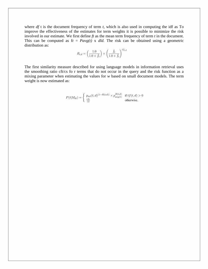
where df t is the document frequency of term t, which is also used in computing the idf as To improve the effectiveness of the estimates for term weights it is possible to minimize the risk

involved in our estimate. We first define ft as the mean term frequency of term t in the document. This can be computed as ft = Pavg(t) x dld. The risk can be obtained using a geometric

distribution as:

The first similarity measure described for using language models in information retrieval uses the smoothing ratio cft/cs fo r terms that do not occur in the query and the risk function as a

mixing parameter when estimating the values for w based on small document models. The term

weight is now estimated as: