lecture notes on discrete mathematics - iitk.ac.in

DRAFT

Lecture Notes on Discrete Mathematics

October 15, 2018

DRAFT

2

DRAFT

Contents

1 Basic Set Theory 5

1.1 Basic Set Theory . . . . . . . . . . . . . . . . . . . . . . . . . . . . . . . . . . . . . . . 5

1.1.1 Union and Intersection of Sets . . . . . . . . . . . . . . . . . . . . . . . . . . . 7

1.1.2 Set Difference, Set Complement and the Power Set . . . . . . . . . . . . . . . . 8

1.2 Relations and Functions . . . . . . . . . . . . . . . . . . . . . . . . . . . . . . . . . . . 9

1.2.1 Composition of Functions . . . . . . . . . . . . . . . . . . . . . . . . . . . . . . 15

1.2.2 Equivalence Relation . . . . . . . . . . . . . . . . . . . . . . . . . . . . . . . . . 16

1.3 Advanced topics in Set Theory and Relations∗ . . . . . . . . . . . . . . . . . . . . . . 19

1.3.1 Families of Sets . . . . . . . . . . . . . . . . . . . . . . . . . . . . . . . . . . . . 19

1.3.2 More on Relations . . . . . . . . . . . . . . . . . . . . . . . . . . . . . . . . . . 21

2 Peano Axioms and Countability 23

2.1 Peano Axioms and the set of Natural Numbers . . . . . . . . . . . . . . . . . . . . . . 23

2.1.1 Addition, Multiplication and its properties . . . . . . . . . . . . . . . . . . . . 24

2.1.2 Well Ordering in N . . . . . . . . . . . . . . . . . . . . . . . . . . . . . . . . . . 26

2.1.3 Applications . . . . . . . . . . . . . . . . . . . . . . . . . . . . . . . . . . . . . 28

2.2 Finite and Infinite Sets . . . . . . . . . . . . . . . . . . . . . . . . . . . . . . . . . . . . 32

2.3 Countable and Uncountable sets . . . . . . . . . . . . . . . . . . . . . . . . . . . . . . 35

2.3.1 Cantor’s Lemma . . . . . . . . . . . . . . . . . . . . . . . . . . . . . . . . . . . 36

2.3.2 Creating Bijections . . . . . . . . . . . . . . . . . . . . . . . . . . . . . . . . . . 37

2.3.3 Schroder-Bernstein Theorem . . . . . . . . . . . . . . . . . . . . . . . . . . . . 39

2.4 Integers and Modular Arithmetic . . . . . . . . . . . . . . . . . . . . . . . . . . . . . . 42

2.5 Construction of Integers and Rationals∗ . . . . . . . . . . . . . . . . . . . . . . . . . . 50

2.5.1 Construction of Integers . . . . . . . . . . . . . . . . . . . . . . . . . . . . . . . 50

2.5.2 Construction of Rational Numbers . . . . . . . . . . . . . . . . . . . . . . . . . 54

3 Partial Orders, Lattices and Boolean Algebra 57

3.1 Partial Orders . . . . . . . . . . . . . . . . . . . . . . . . . . . . . . . . . . . . . . . . . 57

3.2 Lattices . . . . . . . . . . . . . . . . . . . . . . . . . . . . . . . . . . . . . . . . . . . . 65

3.3 Boolean Algebras . . . . . . . . . . . . . . . . . . . . . . . . . . . . . . . . . . . . . . . 71

4 Basic Counting 77

4.1 Permutations and Combinations . . . . . . . . . . . . . . . . . . . . . . . . . . . . . . 78

4.1.1 Multinomial theorem . . . . . . . . . . . . . . . . . . . . . . . . . . . . . . . . . 83

4.2 Circular Permutations . . . . . . . . . . . . . . . . . . . . . . . . . . . . . . . . . . . . 84

4.3 Solutions in Non-negative Integers . . . . . . . . . . . . . . . . . . . . . . . . . . . . . 88

4.4 Set Partitions . . . . . . . . . . . . . . . . . . . . . . . . . . . . . . . . . . . . . . . . . 91

4.5 Lattice Paths and Catalan Numbers . . . . . . . . . . . . . . . . . . . . . . . . . . . . 95

3

DRAFT

4 CONTENTS

4.6 Some Generalizations . . . . . . . . . . . . . . . . . . . . . . . . . . . . . . . . . . . . . 98

5 Advanced Counting Principles 101

5.1 Pigeonhole Principle . . . . . . . . . . . . . . . . . . . . . . . . . . . . . . . . . . . . . 101

5.2 Principle of Inclusion and Exclusion . . . . . . . . . . . . . . . . . . . . . . . . . . . . 104

5.3 Generating Functions . . . . . . . . . . . . . . . . . . . . . . . . . . . . . . . . . . . . . 107

5.4 Recurrence Relation . . . . . . . . . . . . . . . . . . . . . . . . . . . . . . . . . . . . . 116

5.5 Generating Function from Recurrence Relation . . . . . . . . . . . . . . . . . . . . . . 119

6 Introduction to Logic 127

6.1 Propositional Logic . . . . . . . . . . . . . . . . . . . . . . . . . . . . . . . . . . . . . . 127

6.2 Predicate Logic∗ . . . . . . . . . . . . . . . . . . . . . . . . . . . . . . . . . . . . . . . 139

7 Graphs 145

7.1 Basic Concepts . . . . . . . . . . . . . . . . . . . . . . . . . . . . . . . . . . . . . . . . 145

7.2 Connectedness . . . . . . . . . . . . . . . . . . . . . . . . . . . . . . . . . . . . . . . . 151

7.3 Isomorphism in Graphs . . . . . . . . . . . . . . . . . . . . . . . . . . . . . . . . . . . 154

7.4 Trees . . . . . . . . . . . . . . . . . . . . . . . . . . . . . . . . . . . . . . . . . . . . . . 156

7.5 Connectivity . . . . . . . . . . . . . . . . . . . . . . . . . . . . . . . . . . . . . . . . . 161

7.6 Eulerian Graphs . . . . . . . . . . . . . . . . . . . . . . . . . . . . . . . . . . . . . . . 163

7.7 Hamiltonian Graphs . . . . . . . . . . . . . . . . . . . . . . . . . . . . . . . . . . . . . 166

7.8 Bipartite Graphs . . . . . . . . . . . . . . . . . . . . . . . . . . . . . . . . . . . . . . . 169

7.9 Matching in Graphs . . . . . . . . . . . . . . . . . . . . . . . . . . . . . . . . . . . . . 170

7.10 Ramsey Numbers . . . . . . . . . . . . . . . . . . . . . . . . . . . . . . . . . . . . . . . 173

7.11 Degree Sequence . . . . . . . . . . . . . . . . . . . . . . . . . . . . . . . . . . . . . . . 174

7.12 Planar Graphs . . . . . . . . . . . . . . . . . . . . . . . . . . . . . . . . . . . . . . . . 175

7.13 Vertex Coloring . . . . . . . . . . . . . . . . . . . . . . . . . . . . . . . . . . . . . . . . 178

7.14 Representing graphs with Matrices . . . . . . . . . . . . . . . . . . . . . . . . . . . . . 179

7.14.1 More Exercises . . . . . . . . . . . . . . . . . . . . . . . . . . . . . . . . . . . . 180

Index 184

DRAFT

Chapter 1

Basic Set Theory

We will use the following notation throughout the book.

1. The empty set, denoted ∅, is the set that has no element.

2. N := 1, 2, . . ., the set of Natural numbers;

3. W := 0, 1, 2, . . ., the set of whole numbers

4. Z := . . . ,−2,−1, 0, 1, 2, . . ., the set of Integers;

5. Q := pq : p, q ∈ Z, q 6= 0, the set of Rational numbers;

6. R := the set of Real numbers; and

7. C := the set of Complex numbers.

For the sake of convenience, we have assumed that the integer 0, is also a natural number. This chapter

will be devoted to understanding set theory, relations, functions and the principle of mathematical

induction. We start with basic set theory.

1.1 Basic Set Theory

Mathematicians over the last two centuries have been used to the idea of considering a collection of

objects/numbers as a single entity. These entities are what are typically called sets. The technique of

using the concept of a set to answer questions is hardly new. It has been in use since ancient times.

However, the rigorous treatment that the set received happened only in the 19th century due to the

german mathematician Georg Cantor. He was the first person who was responsible in ensuring that

the set had a home in mathematics. Cantor developed the concept of the set during his study of the

trigonometric series, which is now known as the limit point or the derived set operator. He developed

the transfinite numbers of which the ordinals and cardinals are two types. His new and path-breaking

ideas were not well received by his contemporaries. Further, from his definition of a set, a number of

contradictions and paradoxes arose. One of the most famous paradoxes is the Russell’s Paradox, due

to Bertrand Russell in 1918. This paradox amongst others, opened the stage for the development of

axiomatic set theory. The interested reader may refer to Katz [8]. In this book, we will consider the

intuitive or naive view point of sets.

The notion of a set is taken as a primitive and so we will not try to define it explicitly. On the

contrary, we will give it an informal description and then go on to establish the properties of a set.

5

DRAFT

6 CHAPTER 1. BASIC SET THEORY

A set can be described intuitively as a collection of distinct objects. The objects are called the

elements or members of the set. Here, we will be able to say when an object/element belongs to a set

or not.

The objects can be just about anything from real physical things to abstract mathematical objects.

The principal, distinguishable and an important feature of a set is that the objects are “distinct” or

“uniquely identifiable.”

Any object of the collection comprising a set is referred as an element of the set. So, if S is a set

and x is an element of S, we denote it by x ∈ S. If x is not an element of S, we denote it by x 6∈ S.

A set is typically denoted by curly braces, .Example 1.1.1. 1. X = apple, tomato, orange. Hence, orange ∈ X, but potato 6∈ X.

2. X = a1, a2, . . . , a10. Then, a100 6∈ X.

3. Observe that the sets 1, 2, 3, 3, 1, 2 and digits in the number12321 are the same as the

order in which the elements appear doesn’t matter.

We now address the idea of distinctness of elements of a set, which comes with its own subtleties.

Example 1.1.2. 1. Consider a collection of identical red balls in a basket. Is it a set?

2. Consider the list of digits 1, 2, 1, 4, 2. Is it a set?

3. Let X = 1, 2, 3, 4, 5, 6, 7, 8, 9, 10. Then X is the set of first 10 natural numbers. Or equivalently,

X is the set of integers between 0 and 11.

Definition 1.1.3. [Empty Set] The set S that contains no element is called the empty set or the

null set denoted by or ∅.

An object x is an element or a member of a set S, written x ∈ S, if x satisfies the rule that defines

the membership for S. With this notation, one has three main ways for specifying a set. They are:

1. Listing all its elements (list notation), e.g., X = 2, 4, 6, 8, 10. Then X is the set of even integers

between 0 and 12.

2. Stating a property with notation (predicate notation), e.g.,

(a) X = x : x is a prime number. This is read as “X is the set of all x such that x is a prime

number”. Here x is a variable and stands for any object that meets the criteria after the

colon.

(b) The set X = 2, 4, 6, 8, 10 in the predicate notation can be written as

i. X = x : 0 < x ≤ 10, x is an even integer , or

ii. X = x : 1 < x < 11, x is an even integer , or

iii. x = x : 2 ≤ x ≤ 10, x is an even integer etc.

(c) X = x : x is a student in IITK and x is older than 30.

Note that the above expressions are certain rules that help in defining the elements of the set

X. In general, one writes X = x : p(x) or X = x | p(x) to denote the set of all elements x

(variable) such that property p(x) holds. In the above note that “colon” is sometimes replaced

by “—”.

3. Defining a set of rules which generate its members (recursive notation), e.g., let X = x :

x is an even integer greater than 3. Then, X can also be written as

(a) 4 ∈ X.

(b) whenever x ∈ X then x+ 2 ∈ X.

(c) no other element different from those above belongs to X.

DRAFT

1.1. BASIC SET THEORY 7

Thus, in recursive rule, the first rule is the basis of recursion, the second rule gives a method

to generate new element(s) from the elements already determined and the third rule binds or

restricts the defined set to the elements generated by the first two rules. The third rule should

always be there. But, in practice it is left implicit. At this stage, one should make it explicit.

Definition 1.1.4. [Subset and Equality] Let X and Y be two sets.

1. Let Z be a set such that whenever x ∈ Z, x ∈ X as well, then Z is said to be a subset of the

set X, denoted Z ⊆ X.

2. If X ⊆ Y and Y ⊆ X, then X and Y are said to be equal, denoted X = Y .

Example 1.1.5. 1. Let X be a set. Then X ⊆ X. Thus, ∅ ⊆ ∅ and hence the empty set is a

subset of every set.

2. We know that N ⊆W ⊆ Z ⊆ Q ⊆ R ⊆ C.

3. Note that ∅ 6∈ ∅.4. Let X = a, b, c. Then a ∈ X but a ⊆ X. Also, a 6⊆ X.

5. If S ⊆ T and S 6= T then S is called a proper subset of T . That is, there exists an element

a ∈ T such that a 6∈ S.

In the next two subsections, we mention set operations that help us in generating new sets from

existing sets.

1.1.1 Union and Intersection of Sets

Definition 1.1.6. [Set Union and Intersection] Let X and Y be two sets.

1. The union of X and Y , denoted by X ∪ Y , is the set whose elements are the elements of X as

well as the elements of Y . Specifically, X ∪ Y = x | x ∈ X or x ∈ Y .2. The intersection of X and Y , denoted by X ∩ Y , is the set that contains only the common

elements of X and Y . Specifically, X ∩ Y = x | x ∈ X and x ∈ Y . The set X and Y are said

to be disjoint if X ∩ Y = ∅.Example 1.1.7. 1. Let A = 1, 2, 4, 18 and B = x : x is an integer, 0 < x ≤ 5. Then,

A ∪B = 1, 2, 3, 4, 5, 18 and A ∩B = 1, 2, 4.

2. Let S = x ∈ R : 0 ≤ x ≤ 1 and T = x ∈ R : .5 ≤ x < 7. Then,

S ∪ T = x ∈ R : 0 ≤ x < 7 and S ∩ T = x ∈ R : .5 ≤ x ≤ 1.

3. Let A = b, c, b, c, b and B = a, b, c. Then

A ∩B = b and A ∪B = a, b, c, b, c, b, c .

We now state a few properties related to union and intersection of sets. The proof of only the first

distributive law is presented. The readers are supposed to provide proofs of the other results.

Lemma 1.1.8. Let R,S and T be three sets. Then,

1. Obvious properties:

(a) S ∪ T = T ∪ S and S ∩ T = T ∩ S (union and intersection are commutative operations).

(b) R ∪ (S ∪ T ) = (R ∪ S) ∪ T and R ∩ (S ∩ T ) = (R ∩ S) ∩ T (union and intersection are

associative operations).

DRAFT


(c) S ⊆ S ∪ T, T ⊆ S ∪ T .

(d) S ∩ T ⊆ S, S ∩ T ⊆ T .

(e) S ∪ ∅ = S, S ∩ ∅ = ∅.(f) S ∪ S = S ∩ S = S.

2. Distributive laws (combines union and intersection):

(a) R ∪ (S ∩ T ) = (R ∪ S) ∩ (R ∪ T ) (union distributes over intersection).

(b) and R ∩ (S ∪ T ) = (R ∩ S) ∪ (R ∪ T ) (intersection distributes over union).

Proof. Let x ∈ R∪ (S∩T ). Then, x ∈ R or x ∈ S∩T . If x ∈ R then clearly, x ∈ R∪S and x ∈ R∪T .

Thus, x ∈ (R ∪ S) ∩ (R ∪ T ). If x 6∈ R but x ∈ S ∩ T , then x ∈ S and x ∈ T . Hence, x ∈ R ∪ S and

x ∈ R ∪ T . Thus, x ∈ (R ∪ S) ∩ (R ∪ T ). Hence, we see that R ∪ (S ∩ T ) ⊆ (R ∪ S) ∩ (R ∪ T ).

Now, let y ∈ (R ∪ S) ∩ (R ∪ T ). Then, y ∈ R ∪ S and y ∈ R ∪ T . Now, if y ∈ R ∪ S then either

y ∈ R or y ∈ S or both.

If y ∈ R then clearly y ∈ R ∪ (S ∩ T ). If y 6∈ R then the conditions y ∈ R ∪ S and y ∈ R ∪ Timply that y ∈ S and y ∈ T . Thus, y ∈ S ∩ T and hence y ∈ R ∪ (S ∩ T ). This shows that

(R ∪ S) ∩ (R ∪ T ) ⊆ R ∪ (S ∩ T ) and hence we get a complete proof of the first distributive law.

Exercise 1.1.9. 1. Complete the proof of Lemma 1.1.8.

2. Proof the following statements:

(a) S ∪ (S ∩ T ) = S ∩ (S ∪ T ) = S.

(b) S ⊆ T if and only if S ∪ T = T .

(c) If R ⊆ T and S ⊆ T then R ∪ S ⊆ T .

(d) If R ⊆ S and R ⊆ T then R ⊆ S ∩ T .

(e) If S ⊆ T then R ∪ S ⊆ R ∪ T and R ∩ S ⊆ R ∩ T .

(f) If S ∪ T 6= ∅ then either S 6= ∅ or T 6= ∅.(g) If S ∩ T 6= ∅ then both S 6= ∅ and T 6= ∅.(h) S = T if and only if S ∪ T = S ∩ T .

1.1.2 Set Difference, Set Complement and the Power Set

Definition 1.1.10. [Set Difference, Symmetric Difference] Let A and B be two sets.

1. The set difference of X and Y , denoted by X \ Y , is defined by X \ Y = x ∈ X : x 6∈ Y .2. The symmetric difference of X and Y , denoted by X∆Y , is defined by X∆Y = (X \ Y ) ∪

(Y \X).

Example 1.1.11. 1. Let A = 1, 2, 4, 18 and B = x : x is an integer, 0 < x ≤ 5. Then,

A \B = 18, B \A = 3, 5 and A∆B = 3, 5, 18.

2. Let S = x ∈ R : 0 ≤ x ≤ 1 and T = x ∈ R : .5 ≤ x < 7. Then,

S \ T = x ∈ R : 0 ≤ x < .5 and T \ S = x ∈ R : 1 < x < 7.

3. Let A = b, c, b, c, b and B = a, b, c. Then

A \B = b, c, b, c, B \A = a, c and A∆B = a, c, b, c, b, c.

DRAFT

1.2. RELATIONS AND FUNCTIONS 9

In many set theory problems, all sets are defined to be subsets of some reference set, referred to

as the universal set, denoted mostly by U . We now define the complement of a set.

Definition 1.1.12. [Set complement] Let U be the universal set and X ⊆ U . Then, the comple-

ment of X, denoted by X ′, is defined as X ′ = x ∈ U : x 6∈ X.

We now state a few properties that directly follow from the definition and hence the proofs are

omitted.

Lemma 1.1.13. Let U be the universal set and S, T ⊆ U . Then,

1. U ′ = ∅ and ∅′ = U .

2. S ∪ S′ = U and S ∩ S′ = ∅.3. S ∪ U = U and S ∩ U = S.

4. (S′)′ = S.

5. S ⊆ S′ if and only if S = ∅.6. S ⊆ T if and only if T ′ ⊆ S′.7. S = T ′ if and only if S ∩ T = ∅andS ∪ T = U .

8. S \ T = S ∩ T ′ and T \ S = T ∩ S′.9. S∆T = (S ∪ T ) \ (S ∩ T ).

10. De-Morgan’s Laws:

(a) (S ∪ T )′ = S′ ∩ T ′.(b) (S ∩ T )′ = S′ ∪ T ′.

The De-Morgan’s laws help us to convert arbitrary set expressions into those that involve only

complements and unions or only complements and intersections.

Definition 1.1.14. [Power Set] Let X be a subset of a set Ω. Then the set that contains all subsets

of X is called the power set of X and is denoted by P(X) or 2X .

Example 1.1.15. 1. Let X = ∅. Then P(∅) = ∅, X = ∅.

2. Let X = ∅. Then P(X) = ∅, X = ∅, ∅.

3. Let X = a, b, c. Then P(X) = ∅, a, b, c, a, b, a, c, b, c, a, b, c.

4. Let X = b, c, b, c. Then P(X) = ∅, b, c, b, c, b, c, b, c .

1.2 Relations and Functions

We start with the definition of the cartesian product of two sets and use it to define relations. Note

that this is another method to construct new sets from given set(s).

Definition 1.2.1. [Cartesian Product] Let X and Y be two sets. Then their cartesian product,

denoted by X × Y , is defined as X × Y = (a, b) : a ∈ X, b ∈ Y . Thus,

(a1, b1) = (a2, b2) if and only if a1 = a2 and b1 = b2.

Example 1.2.2. 1. Let A = a, b, c and B = 1, 2, 3, 4. Then

A×A = (a, a), (a, b), (a, c), (b, a), (b, b), (b, c), (c, a), (c, b), (c, c).A×B = (a, 1), (a, 2), (a, 3), (a, 4), (b, 1), (b, 2), (b, 3), (b, 4), (c, 1), (c, 2), (c, 3), (c, 4).

DRAFT


2. The Euclidean plane, denoted by R2 = R× R = (x, y) : x, y ∈ R.

3. By convention, ∅ ×B = A× ∅ = ∅. In fact, A×B = ∅ if and only if A = ∅ or B = ∅.

4. One can use the product construction several times, e.g., if X,Y and Z are sets then

X × Y × Z = (x, y, z) : x ∈ X, y ∈ Y, z ∈ Z = (X × Y )× Z = X × (Y × Z).

Exercise 1.2.3. Let A,B,C and D be non-empty sets. Then, prove the following statements:

1. A× (B ∪ C) = (A×B) ∪ (A× C).

2. A× (B ∩ C) = (A×B) ∩ (A× C).

3. (A×B) ∩ (C ×D) = (A ∩ C)× (B ∩D).

4. (A× B) ∪ (C ×D) ⊆ (A ∪ C)× (B ∪D). Give an example to show that the converse need not

be true.

Definition 1.2.4. [Relation] Let X and Y be two non-empty sets. A relation R from X to Y is a

subset of X × Y . We write xRy to mean (x, y) ∈ R ⊆ X × Y . Thus, for any two sets X and Y , the

sets ∅ and X × Y are always relations from X to Y . A relation from X to X is called a relation on

X.

Example 1.2.5. 1. Let X be any non-empty set and consider the set P(X). Then one can define

a relation R on P(X) by R = (S, T ) ∈ P(X)× P(X) : S ⊆ T.

2. Let A = a, b, c, d. Then, some of the relations R on A are:

(a) R = A×A.

(b) R = (a, a), (b, b), (c, c), (d, d), (a, b), (a, c), (b, c).

(c) R = (a, a), (b, b), (c, c).

(d) R = (a, a), (a, b), (b, a), (b, b), (c, d).

(e) R = (a, a), (a, b), (b, a), (a, c), (c, a), (c, c), (b, b).

(f) R = (a, b), (b, c), (a, c), (d, d).

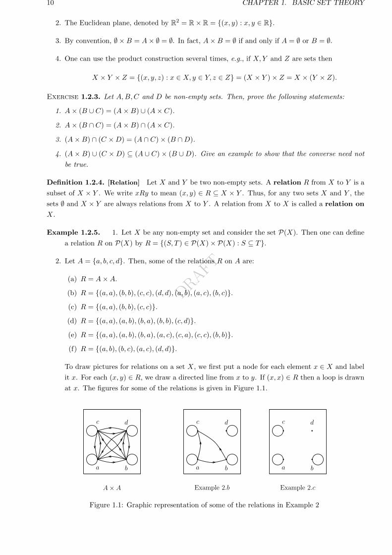
To draw pictures for relations on a set X, we first put a node for each element x ∈ X and label

it x. For each (x, y) ∈ R, we draw a directed line from x to y. If (x, x) ∈ R then a loop is drawn

at x. The figures for some of the relations is given in Figure 1.1.

a b

c d

A × A

a b

c d

Example 2.b

a b

c d

Example 2.c

1

Figure 1.1: Graphic representation of some of the relations in Example 2

DRAFT


1

3

2

a

b

c

R

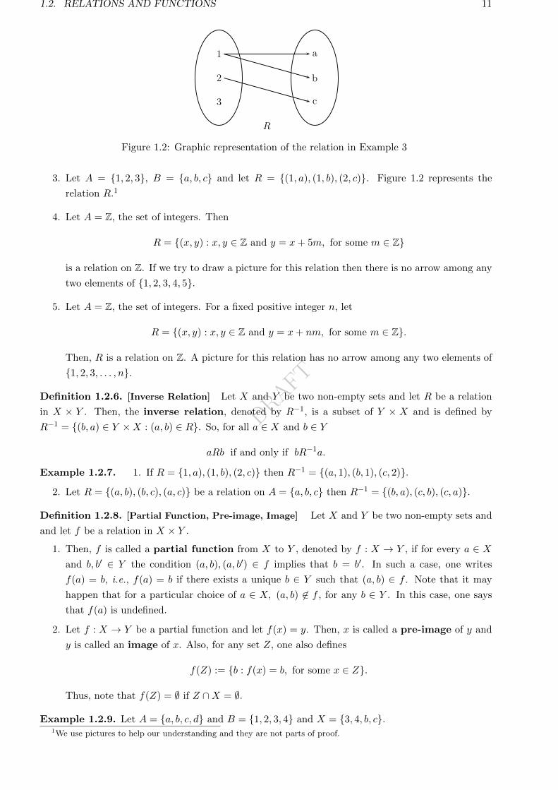
Figure 1.2: Graphic representation of the relation in Example 3

3. Let A = 1, 2, 3, B = a, b, c and let R = (1, a), (1, b), (2, c). Figure 1.2 represents the

relation R.1

4. Let A = Z, the set of integers. Then

R = (x, y) : x, y ∈ Z and y = x+ 5m, for some m ∈ Z

is a relation on Z. If we try to draw a picture for this relation then there is no arrow among any

two elements of 1, 2, 3, 4, 5.

5. Let A = Z, the set of integers. For a fixed positive integer n, let

R = (x, y) : x, y ∈ Z and y = x+ nm, for some m ∈ Z.

Then, R is a relation on Z. A picture for this relation has no arrow among any two elements of

1, 2, 3, . . . , n.

Definition 1.2.6. [Inverse Relation] Let X and Y be two non-empty sets and let R be a relation

in X × Y . Then, the inverse relation, denoted by R−1, is a subset of Y × X and is defined by

R−1 = (b, a) ∈ Y ×X : (a, b) ∈ R. So, for all a ∈ X and b ∈ Y

aRb if and only if bR−1a.

Example 1.2.7. 1. If R = 1, a), (1, b), (2, c) then R−1 = (a, 1), (b, 1), (c, 2).2. Let R = (a, b), (b, c), (a, c) be a relation on A = a, b, c then R−1 = (b, a), (c, b), (c, a).

Definition 1.2.8. [Partial Function, Pre-image, Image] Let X and Y be two non-empty sets and

and let f be a relation in X × Y .

1. Then, f is called a partial function from X to Y , denoted by f : X → Y , if for every a ∈ Xand b, b′ ∈ Y the condition (a, b), (a, b′) ∈ f implies that b = b′. In such a case, one writes

f(a) = b, i.e., f(a) = b if there exists a unique b ∈ Y such that (a, b) ∈ f . Note that it may

happen that for a particular choice of a ∈ X, (a, b) 6∈ f , for any b ∈ Y . In this case, one says

that f(a) is undefined.

2. Let f : X → Y be a partial function and let f(x) = y. Then, x is called a pre-image of y and

y is called an image of x. Also, for any set Z, one also defines

f(Z) := b : f(x) = b, for some x ∈ Z.

Thus, note that f(Z) = ∅ if Z ∩X = ∅.

Example 1.2.9. Let A = a, b, c, d and B = 1, 2, 3, 4 and X = 3, 4, b, c.1We use pictures to help our understanding and they are not parts of proof.

DRAFT


1. If R1 = (a, 1), (b, 1), (c, 2) is a relation in A×B then

(a) R1 is a partial function.

(b) R1(a) = 1, R1(b) = 1, R1(c) = 2. Also, R1(d) is undefined. Thus, R1(d) = ∅.(c) R1(X) = 1, 2.(d) R−11 (1) = a, b and R−11 (2) = c as R−11 = (1, a), (1, b), (2, c). For x ∈ X, R−11 (x) is

not defined and hence R−11 (X) = ∅.

2. If R2 = (a, 1), (b, 4), (c, 2), (d, 3) is a relation in A×B then

(a) R2 is a partial function.

(b) R2(a) = 1, R2(b) = 4, R2(c) = 2 and R2(d) = 3.

(c) R2(X) = 2, 4.(d) R−12 (1) = a, R−12 (2) = c, R−12 (3) = d and R−12 (4) = b. Also, R−12 (X) = b, d.

Definition 1.2.10. [Domain, Range, Function] Let X and Y be two non-empty sets and let

f : X → Y be a partial function.

1. Then, the domain 1 of f , denoted by dom f := a : (a, b) ∈ f is the set of all pre-images of f .

2. Then, the range of f , denoted by rng f := b : (a, b) ∈ f is the collection of images of f .

3. If dom f = X then the partial function f is called a total function on X, or a function from

X to Y .

Convention:

Let p(x) be a polynomial in x with integer coefficients. Then, by writing ‘f : Z→ Z is a function

defined by f(x) = p(x)’, we mean the function f = (a, p(a)) : a ∈ Z. For example, the function

f(x) = x2 stands for the set (a, a2) : a ∈ Z.Example 1.2.11. 1. For A = a, b, c, d and B = 1, 3, 5, let f = (a, 5), (b, 1), (d, 5) be a

relation in A × B. Then, f is a partial function with dom f = a, b, d and rng f = 1, 5.Further, we can define a function g : a, b, d → 1, 5 by g(a) = 5, g(b) = 1 and g(d) = 5. Also,

using g, one obtains the relation g−1 = (1, b), (5, a), (5, d).2. Note that the following relations f : Z→ Z are indeed functions.

(a) f = (x, 1) | x is even ∪ (x, 5) | x is odd.(b) f = (x,−1) | x ∈ Z.(c) f = (x, x (mod 10)) | x ∈ Z, where x (mod 10) gives the remainder when 10 divides x.

(d) f = (x, 1) | x < 0 ∪ (0, 0) ∪ (x,−1) | x > 0.

Remark 1.2.12. 1. If X = ∅, then by convention, one assumes that there is a function, called the

empty function, from X to Y .

2. If Y = ∅, then it can be easily observed that there is no function from X to Y .

3. Individual relations and functions are also sets. Therefore, one can have equality between re-

lations and functions, i.e., they are equal if and only if they contain the same set of pairs.

For example, let A = −1, 0, 1. Then, the functions f, g, h : A → A defined by f(x) =

x, g(x) = x|x| and h(x) = x3 are equal as the three functions correspond to the relation R =

(−1,−1), (0, 0), (1, 1) on A.

1The domain set is the set from which we define our relations but dom f is the domain of the particular partial

function f . They are different.

DRAFT


4. Some books use the word ‘map’ in place of ‘function’. So, both the words are used interchangeably

throughout the book.

5. Throughout the book, whenever the phrase ‘let f : X → Y be a function’ is used, it will be

assumed that both X and Y are nonempty sets.

The following is an immediate consequence of the definition.

Proposition 1.2.13. Let f be a non-empty relation in A×B and S be any set. Then,

1. f(S) 6= ∅ if and only if dom(f) ∩ S 6= ∅.2. f−1(S) 6= ∅ if and only if rng(f) ∩ S 6= ∅.

Proof. We will prove only one way implication. The other way is left for the reader.

Part 1: Since f(S) 6= ∅, one can find a ∈ S ∩A and b ∈ B such that (a, b) ∈ f . This, in turn, implies

that a ∈ dom(f) ∩ S (a ∈ S).

Part 2: Since rng(f) ∩ S 6= ∅, one can find b ∈ rng(f) ∩ S and a ∈ A such that (a, b) ∈ f . This, in

turn, implies that a ∈ f−1(b) ⊆ f−1(S).

Some important functions are now defined.

Definition 1.2.14. [Identity and Zero functions] Let X be a non-empty set.

1. Then the relation Id := (x, x) : x ∈ X is called the identity relation on X.

2. Then the function f : X → X defined by f(x) = x, for all x ∈ X, is called the identity function

and is denoted by Id.

3. Then the function f : X → R with f(x) = 0, for all x ∈ X, is called the zero function and is

denoted by 0.

Exercise 1.2.15. 1. Do the following relations represent functions? If yes, why?

(a) Let f : Z→ Z be defined by

i. f = (x, 1) | 2 divides x ∪ (x, 5) | 3 divides x.ii. f = (x, 1) | x ∈ S ∪ (x,−1) | x ∈ S′, where S = n2 : n ∈ Z and S′ = Z \ S.

iii. f = (x, x3) | x ∈ Z.(b) Let f : R+ → R be defined by f = (x,±√x) | x ∈ R+.(c) Let f : R→ R be defined by f = (x,√x) | x ∈ R.(d) Let f : R→ C be defined by f = (x,√x) | x ∈ R.(e) Let f : R∗ → R be defined by f = (x, loge |x|) | x ∈ R∗.(f) Let f : R→ R be defined by f = (x, tanx) | x ∈ R.

2. Let f : X → Y be a function. Then f−1 is a relation in Y ×X and the following results hold

for f−1.

(a) f−1(A ∪B) = f−1(A) ∪ f−1(B), for each A,B ⊆ Y .

(b) f−1(A ∩B) = f−1(A) ∩ f−1(B), for each A,B ⊆ Y .

(c) f−1(∅) = ∅.(d) f−1(Y ) = X.

(e) f−1(B′) =(f−1(B)

)′, for each B ⊆ Y , where B′ is the complement of B in Y and(

f−1(B))′

is the complement of f−1(B) in X.

DRAFT


Definition 1.2.16. [One-one/Injection] A function f : X → Y is called one-one (also called an

injection), if f(x) 6= f(y) is true for each pair x 6= y in X. Equivalently, f is one-one if x = y is true

for each pair x, y ∈ X for which f(x) = f(y).

Example 1.2.17. 1. Let A be a non-empty set. Then the identity map, Id, is one-one.

2. Let ∅ 6= A ( B. Then f(x) = x is a one-one map from A to B.

3. The function f : Z→ Z defined by f(x) = x2 is not one-one as f(−1) = f(1) = 1.

4. The function f : 1, 2, 3 → a, b, c, d defined by f(1) = c, f(2) = b and f(3) = a, is one-one.

It can be checked that there are 24 one-one functions f : 1, 2, 3 → a, b, c, d.5. There is no one-one function from the set 1, 2, 3 to its proper subset 1, 2.6. There are one-one functions from the set N of natural numbers to its proper subset 2, 3, . . ..

One of them is given by f(1) = 4, f(2) = 3, f(3) = 2 and f(n) = n+ 1, for all n ≥ 4.

Definition 1.2.18. [Restriction function] Let f : X → Y be a function and A ⊆ X, A 6= ∅. Then,

by fA, we denote the function fA = (x, y) : (x, y) ∈ f, x ∈ A, called the restriction of f to A.

Example 1.2.19. Define f : R → R as f(x) = 1, if x is irrational and f(x) = 0, if x is rational.

Then, fQ : Q→ R is the constant 0 function.

Proposition 1.2.20. Let f : X → Y be a one-one function and Z be a nonempty subset of X. Then,

fZ is also one-one.

Proof. Let if possible, fZ(x) = fZ(y), for some x, y ∈ Z. Then, by definition of fZ , we have

f(x) = f(y). As f is one-one, we get x = y. Thus, fZ is one-one.

Definition 1.2.21. [Onto/Surjection] A function f : X → Y is called onto (also called a sur-

jection), if f−1(b) 6= ∅, for each b ∈ Y . Equivalently, f : X → Y is onto if ‘each b ∈ Y has some

pre-image in X’.

Example 1.2.22. 1. Let A be a non-empty set. Then the identity map, Id, is onto.

2. Let ∅ 6= A ( B. Then f(x) = x is a not onto as A ( B.

3. There are 6 onto functions from 1, 2, 3 to 1, 2. For example, f(1) = 1, f(2) = 2, and f(3) = 2

is one such function.

4. Let ∅ 6= A ( B. Choose a ∈ A. Then g(y) =

y, if y ∈ A,a, if y ∈ B \A.

is an onto map from B to A.

5. There is no onto function from the set 1, 2 to its proper superset 1, 2, 3.6. There are onto functions from the set 2, 3, . . . to its proper superset N, the set of natural

numbers. One of them is given by f(n) = n− 1, for all n ≥ 2.

Definition 1.2.23. [Bijection/One-One Correspondence, Equivalent Set] Let X and Y be two

sets. A function f : X → Y is said to be a bijection if f is one-one as well as onto. The sets X and

Y are said to be equivalent if there exists a bijection f : X → Y .

Example 1.2.24. 1. The function f : 1, 2, 3 → a, b, c defined by f(1) = c, f(2) = b and

f(3) = a, is a bijection. Thus, the set a, b, c is equivalent to 1, 2, 3.2. Let A be a non-empty set. Then the identity map, Id, is a bijection. Thus, the set A is equivalent

to itself.

3. The set N is equivalent to 2, 3, . . .. Indeed the function f : N → 2, 3, . . . defined by f(1) =

3, f(2) = 2 and f(n) = n+ 1, for all n ≥ 3 is a bijection.

DRAFT


Exercise 1.2.25. 1. Define f : N ∪ 0 → Z by f = (x, −x2

)| x is even ∪

(x, x+1

2

)| x is odd.

Is f one-one? Is it onto?

2. Define f : N→ Z and g : Z→ Z by f = (x, 2x) | x ∈ N and g = (x, x2

)| x is even ∪ (x, 0) |

x is odd. Are f and g one-one? Are they onto?

3. Let A be the class of subsets of 1, 2, . . . , 9 of size 5 and B be the class of 5 digit numbers with

strictly increasing digits. For a ∈ A, define f(a) the number obtained by arranging the elements

of a in increasing order. Is f one-one and onto?

1.2.1 Composition of Functions

Definition 1.2.26. [Composition of relations] Let f and g be two relations such that rng f ⊆ dom g.

Then, the composition of f and g, denoted by g f , is defined as

g f =

(x, z) : (x, y) ∈ f and (y, z) ∈ g for some y ∈ rng(f) ⊆ dom(g).

It is a relation. In case, both f and g are functions then (g f)(x) = g (f(x)) as (x, z) ∈ g f implies

that there exists y such that y = f(x) and z = g(y). Similarly, one defines f g if rng g ⊆ dom f .

Example 1.2.27. Take f = (β, a), (3, b), (3, c) and g = (a, 3), (b, β), (c, β). Then, g f =

(3, β), (β, 3) and f g = (a, b), (a, c), (b, a), (c, a).

The proof of the next result is omitted as it directly follows from definition.

Proposition 1.2.28. [Algebra of composition of functions] Let f : A → B, g : B → C and

h : C → D be functions.

1. Then, (h g)f : A→ D and h(g f) : A→ D are functions. Moreover, (h g)f = h(g f)

(associativity holds).

2. If f and g are injections then g f : A→ C is an injection.

3. If f and g are surjections then g f : A→ C is a surjection.

4. If f and g are bijections then g f : A→ C is a bijection.

5. [Extension] If dom f ∩ domh = ∅ and rng f ∩ rng h = ∅ then the function f ∪ h from A ∪ C to

B ∪D defined by f ∪ h = (a, f(a)) : a ∈ A ∪ (c, h(c)) : c ∈ C is a bijection.

6. Let A and B be sets with at least two elements each and let f : A→ B be a bijection. Then, the

number of bijections from A to B is at least 2.

Theorem 1.2.29. [Properties of identity function] Let A and B be two nonempty sets and Id :

A→ A be the identity function. Then, for any two functions f : A→ B and g : B → A

1. the map f Id = f .

2. the map Id g = g.

Proof. Part 1: By definition, (f Id)(a) = f(Id(a)) = f(a), for all a ∈ A. Hence, f Id = f .

Part 2: The readers are advised to supply the proof.

We now give a very important bijection principle.

Theorem 1.2.30. [bijection principle] Let f : A → B and g : B → A be functions such that

g f(a) = a, for each a ∈ A. Then

DRAFT


1. f is one-one and

2. g is onto.

Proof. Let g f(a) = a, for each a ∈ A. To prove the first part, let us assume that f(a1) = f(a2), for

some a1, a2 ∈ A. Then using the given condition

a1 = g f(a1) = g (f(a1)) = g (f(a2)) = g f(a2) = a2.

Thus, f is one-one and this completes the proof of the first.

For the second part, let a ∈ A. As g f(a) = a, we see that for b = f(a), one has g(b) = g(f(a)) =

g f(a) = a. Thus, we have found b ∈ B such that g(b) = a. Hence, g is onto and this completes the

required proof.

Exercise 1.2.31. 1. Let f, g : N → N be defined by f = (x, 2x) | x ∈ N and g = (x, x2

)|

x is even ∪ (x, 0) | x is odd. Then, verify that g f is the identity map on N, whereas f gmaps even numbers to itself and maps odd numbers to 0.

2. Let f : X → Y be a function. Then, prove that f−1 : Y → X is a function if and only if f is a

bijection.

3. Define f : N× N→ N by f(m,n) = 2m−1(2n− 1). Is f a bijection?

4. Let f : X → Y be a bijection and A ⊆ X. Is f(A′) = (f(A))′?

5. Let f : X → Y and g : Y → X be two functions such that

(a) (f g)(y) = y holds, for each y ∈ Y .

(b) (g f)(x) = x holds, for each x ∈ X.

Show that f is a bijection and g = f−1. Can we conclude the same without assuming the second

condition?

1.2.2 Equivalence Relation

Now that we have seen quite a few examples of relations, let us look at some of the properties that

are of interest in mathematics.

Definition 1.2.32. [Relations on Set] Let R be a relation on a non-empty set A. Then R is said

to be

1. reflexive if (a, a) ∈ R, for all a ∈ A.

2. symmetric if (b, a) ∈ R whenever (a, b) ∈ R.

3. anti-symmetric if, for all a, b ∈ A with (a, b), (b, a) ∈ R implies a = b in A.

4. transitive if, for all a, b, c ∈ A with (a, b), (b, c) ∈ R implies (a, c) ∈ R.

Exercise 1.2.33. For relations defined in Example 1.2.5, determine which of them are

1. reflexive.

2. symmetric.

3. anti-symmetric.

4. transitive.

DRAFT


We are now ready to define a relation that appears quite frequently in mathematics. Before doing

so, let us either use the symbol ∼ orR∼ for relation. That is, if a, b ∈ A then we represent (a, b) ∈ R

by either a ∼ b or aR∼ b.

Definition 1.2.34. [Equivalence Relation, Equivalence Class] Let ∼ be a relation on a non-empty

set A. Then ∼ is said to form an equivalence relation if ∼ is reflexive, symmetric and transitive.

The equivalence class containing a ∈ A, denoted [a], is defined as [a] := b ∈ A : b ∼ a.Example 1.2.35. 1. Consider the relations on A that appear in Example 1.2.5. Then,

(a) Example 1.2.5.1 is not an equivalence relation (the relation is not symmetric).

(b) Example 1.2.5.2.2a is an equivalence relation with [a] = a, b, c, d as the only equivalence

class.

(c) Other relations in Example 1.2.5.2 are not equivalence relation.

(d) Example 1.2.5.4 is an equivalence relation with the equivalence classes as

i. [0] = . . . ,−15,−10,−5, 0, 5, 10, . . ..ii. [1] = . . . ,−14,−9,−4, 1, 6, 11, . . ..iii. [2] = . . . ,−13,−8,−3, 2, 7, 12, . . ..iv. [3] = . . . ,−12,−7,−2, 3, 8, 13, . . ..v. [4] = . . . ,−11,−6,−1, 4, 9, 14, . . ..

(e) Example 1.2.5.5 is an equivalence relation with the equivalence classes as

i. [0] = . . . ,−3n,−2n,−n, 0, n, 2n, . . ..ii. [1] = . . . ,−3n+ 1,−2n+ 1,−n+ 1, 1, n+ 1, 2n+ 1, . . ..iii. [2] = . . . ,−3n+ 2,−2n+ 2,−n+ 2, 2, n+ 2, 2n+ 2, . . ..iv. [n− 2] = . . . ,−2n− 2,−n− 2,−2, n− 2, 2n− 2, 3n− 2, . . ..v. [n− 1] = . . . ,−2n− 1,−n− 1,−1, n− 1, 2n− 1, 3n− 1, . . ..

2. Let R = (a, a), (b, b), (c, c) be a relation on A = a, b, c. Then, R forms an equivalence relation

with three equivalence classes, namely [a] = a, [b] = b and [c] = c.3. Let R = (a, a), (b, b), (c, c), (a, c), (c, a) be a relation on A = a, b, c. Then, R forms an

equivalence relation with two equivalence classes, namely [a] = [c] = a, c and [b] = b.

Proposition 1.2.36. [Equivalence relation divides a set into disjoint classes] Let ∼ be an equiva-

lence relation on X.

1. Then any two equivalence classes are either disjoint or identical.

2. Further, X =⋃a∈X

[a].

Thus, an equivalence relation ∼ on X divides X into disjoint equivalence classes.

Proof. If the equivalence classes [a] and [b] are disjoint, then there is nothing to prove. So, let us

assume that there are two equivalence classes, say [a] and [b], that intersect. Hence, there exists c ∈ Xsuch that c ∈ [a] ∩ [b]. That is, c ∼ a and c ∼ b.

As ∼ is symmetric, a ∼ c as well. Now, ∼ is transitive, with a ∼ c and c ∼ b and so a ∼ b. Hence,

if x ∼ a, then the above argument implies that x ∼ b. Thus, [a] ⊆ [b]. A similar argument implies

that [b] ⊆ [a] as symmetry with c ∼ b implies b ∼ c and the transitivity with b ∼ c and c ∼ a implies

b ∼ a. Thus, whenever two equivalence classes intersect, they are indeed equal.

For the second part, note that for each x ∈ X, [x], the equivalence class containing x is well

defined. Thus, if we take the union over all x ∈ X, we get X =⋃x∈X

[x].

DRAFT


Exercise 1.2.37. Determine the equivalence relation among the relations given below. Further, for

each equivalence relation, determine its equivalence classes.

1. R = (a, b) ∈ Z2 | a ≤ b on Z?

2. R = (a, b) ∈ Z∗ × Z∗ | a divides b, where Z∗ = Z \ 0 on Z∗?

3. For x = (x1, x2),y = (y1, y2) ∈ R2 and R∗ = R \ 0, let

(a) R = (x,y) ∈ R2 × R2 | |x|2 = x21 + x22 = y21 + y22 = |y|2.(b) R = (x,y) ∈ R2 × R2 | x = αy for some α ∈ R∗.(c) R = (x,y) ∈ R2 × R2 | 4x21 + 9x22 = 4y21 + 9y22.(d) R = (x,y) ∈ R2 × R2 | x− y = α(1, 1) for some α ∈ R∗.(e) Fix c ∈ R. Now, define R = (x,y) ∈ R2 × R2 | y2 − x2 = c(y1 − x1).(f) R = (x,y) ∈ R2 × R2 | |x1|+ |x2| = α(|y1|+ |y2|), for some positive real number α.

(g) R = (x,y) ∈ R2 × R2 | x1x2 = y1y2.

4. For x = (x1, x2),y = (y1, y2) ∈ R2, let S = x ∈ R2 | x21 + x22 = 1. Then is the relation given

below an equivalence relation on S?

(a) R = (x,y) ∈ S × S | x1 = y1, x2 = −y2.(b) R = (x,y) ∈ S × S | x = −y.

Definition 1.2.38. [Partition of a set] Let X be a non-empty set. Then a partition of X is a

collection of disjoint, non-empty subsets of X whose union is X.

Example 1.2.39. Let X = a, b, c, d, e.1. If R is an equivalence relation on X with

R = (a, a), (b, b), (c, c), (d, d), (e, e), (a, b), (b, a), (c, e), (e, c)

then its equivalence classes are [a] = [b] = a, b, [c] = [e] = c, e and [d] = d.2. Let a, b, c, d, e be a partition of X. Then verify that

R = (a, a), (b, b), (c, c), (d, d), (e, e), (b, c), (c, d), (b, d), (c, b), (d, c), (d, b)

is an equivalence relation with [a] = a, [b] = b, c, d and [e] = e.

The next proposition follows directly follows from Proposition 1.2.36 and hence the proof is omitted.

It answers the question that “if a partition of a non-empty set X is given then does there exists an

equivalence relation on X such that the disjoint equivalence classes are exactly the elements of the

partition?”

Proposition 1.2.40. [Constructing equivalence relation from equivalence classes] Let f be an

equivalence relation on X 6= ∅ whose disjoint equivalence classes are [a] : a ∈ A, for some index set

A. Then,

f =

(⋃x∈X(x, x)

)⋃(⋃a∈A(x, y) : x, y ∈ [a], x 6= y

).

Exercise 1.2.41. 1. Let X and Y be two nonempty sets and f : X → Y be a relation. Let IdX

and IdY be the identity relations on X and Y , respectively. Then,

(a) is it necessary that f−1 f ⊆ IdX?

(b) is it necessary that f−1 f ⊇ IdX?

DRAFT

1.3. ADVANCED TOPICS IN SET THEORY AND RELATIONS∗ 19

(c) is it necessary that f f−1 ⊆ IdY ?

(d) is it necessary that f f−1 ⊇ IdY ?

2. Suppose now that f is a function. Then,

(a) is it necessary that f f−1 ⊆ IdY ?

(b) is it necessary that IdX ⊆ f−1 f?

3. Take A 6= ∅. Is A×A an equivalence relation on A? If yes, what are the equivalence classes?

4. On a nonempty set A, what is the smallest equivalence relation (in the sense that every other

equivalence relation will contain this equivalence relation; recall that a relation is a set)?

Exercise 1.2.42. [Optional]

1. Let X = 1, 2, 3, 4, 5 and let f be a relation on X. By checking whether f is reflexive or not,

whether f is symmetric or not and whether f is transitive or not, we see that there are 8 types

of relations on X. Give one example for each type.

2. Let A = B = 1, 2, 3. Then, what is the number of

(a) relations from A to B?

(b) relations f from 1, 2, 3 to a, b, c such that dom f = 1, 3?(c) relations f from 1, 2, 3 to itself such that f = f−1?

(d) single valued relations from 1, 2, 3 to itself? How many of them are functions?

(e) equivalence relations on 1, 2, 3, 4, 5.

3. Let f, g be two non-equivalence relations on R. Then, is it possible to have f g as an equivalence

relation? Give reasons for your answer.

4. Let f, g be two equivalence relations on R. Then, prove/disprove the following statements.

(a) f g is necessarily an equivalence relation.

(b) f ∩ g is necessarily an equivalence relation.

(c) f ∪ g is necessarily an equivalence relation.

(d) f ∪ g′ is necessarily an equivalence relation.

1.3 Advanced topics in Set Theory and Relations∗

1.3.1 Families of Sets

Definition 1.3.1. [Family of sets] Let A be a set. For each x ∈ A, take a new set Ax. Then, the

collection

Axx∈A :=Ax | x ∈ A

is a family of sets indexed by elements of A (index set). Unless otherwise mentioned, we assume

that the index set for a class of sets is nonempty.

Definition 1.3.2. [Union / Intersection of families of sets] Let Bαα∈S be a nonempty class of

sets. We define their

1. union as ∪α∈S

Bα = x | x ∈ Bα, for some α, and

2. intersection as ∩α∈S

Bα = x | x ∈ Bα, for all α.

DRAFT


[Convention] Union of an empty class is ∅. The intersection of an empty class of subsets of a set X

is X1.

Example 1.3.3. 1. Take A = 1, 2, 3, A1 = 1, 2, A2 = 2, 3 and A3 = 4, 5. Then,

Aα | α ∈ A = A1, A2, A3 =1, 2, 2, 3, 4, 5

.

Thus, ∪α∈A

Aα = 1, 2, 3, 4, 5 and ∩α∈A

Aα = ∅.

2. Take A = N and An = n, n+ 1, . . .. Then, the family

Aα | α ∈ A = A1, A2, . . . =1, 2, . . ., 2, 3, . . ., . . .

.

Thus, ∪α∈A

Aα = N and ∩α∈A

Aα = ∅.

3. Verify that⋂n∈N

[− 1n ,

2n ] = 0.

We now give a set of important rules some of whose proofs are left for the reader.

Theorem 1.3.4. [Algebra of union and intersection] Let Aαα∈L be a nonempty class of subsets

of X and B be any set. Then, the following statements are true.

1. B ∩(∪α∈L

Aα

)= ∪

α∈L(B ∩Aα).

2. B ∪(∩α∈L

Aα

)= ∩

α∈L(B ∪Aα).

3.(∪α∈L

Aα)′

= ∩α∈L

A′α.

4.(∩α∈L

Aα)′

= ∪α∈L

A′α.

Proof. We give the proofs for Part 1 and 4. For Part 1, we see that

x ∈ B ∩(∪α∈L

Aα

)⇔ x ∈ B and x ∈ ∪

α∈LAα ⇔ x ∈ B and x ∈ Aα, for some α ∈ L

⇔ x ∈ B ∩Aα, for some α ∈ L⇔ x ∈ ∪α∈L

(B ∩Aα).

For Part 4, we have

x ∈(∩α∈L

Aα)′ ⇔ x 6∈ ∩

α∈LAα ⇔ x 6∈ Aα, for some α ∈ L⇔ x ∈ A′α, for some α ∈ L

⇔ x ∈ ∪α∈L

A′α.

Proceed in similar lines to complete the proofs of the other parts.

Exercise 1.3.5. 1. ConsiderAxx∈R, where Ax = [x, x+ 1]. What is ∪

x∈RAx and ∩

x∈RAx?

2. For x ∈ [0, 1] write Zx := zx | z ∈ Z and Ax = R \ Zx. What is ∪x∈R

Ax and ∩x∈R

Ax?

3. Write the closed interval [1, 2] = ∩n∈N

In, where In are open intervals.

4. Write R as a union of infinite number of pairwise disjoint infinite sets.

5. Write the set 1, 2, 3, 4 as the intersection of infinite number of infinite sets.

6. Suppose that A∆B = B. Is A = ∅?7. Prove Theorem 1.3.4.1The way we see this convention is as follows: First we agree that the intersection of an empty class of subsets is a

subset of X. Now, let x ∈ X such that x 6∈ ∩α∈S

Bα. This implies that there exists an α ∈ S such that x 6∈ Bα. Since S

is empty, such an α does not exist.

DRAFT

1.3. ADVANCED TOPICS IN SET THEORY AND RELATIONS∗ 21

1.3.2 More on Relations

Proposition 1.3.6. [Properties of union and intersection under a relation] Let f : X → Y be a

relation and Aαα∈L ⊆ P(X). Then, the following statements hold.

1. f(∪α∈L

Aα)

= ∪α∈L

f(Aα).

2. f(∩α∈L

Aα)⊆ ∩

α∈Lf(Aα). Give an example where the inclusion is strict.

Proof. Part 1:

y ∈ f(∪α∈L

Aα)⇔ (x, y) ∈ f, for some x ∈ ∪

α∈LAα ⇔ (x, y) ∈ f with x ∈ Aα, for some α ∈ L

⇔ y ∈ f(Aα), for some α ∈ L⇔ y ∈ ∪α∈L

f(Aα).

For Part 2, we assume that ∩α∈L

Aα 6= ∅. Then,

y ∈ f(∩α∈L

Aα)⇔ (x, y) ∈ f, for some x ∈ ∩

α∈LAα ⇔ (x, y) ∈ f with x ∈ Aα, for all α ∈ L

⇒ y ∈ f(Aα), for all α ∈ L⇔ y ∈ ∩α∈L

f(Aα).

Thus, the required result follows.

Remark 1.3.7. It is important to note the following in the proof of the above theorem:

‘y ∈ f(Aα), for all α ∈ L’ implies that ‘for each α ∈ L, we can find some xα ∈ Aα such that (xα, y) ∈f ’. That is, the xα’s need not be the same. This gives you an idea to construct a counterexample.

Define f : 1, 2, 3, 4 → a, b by f = (1, a), (2, a), (2, b), (3, b), (4, b). Take A1 = 1, 3 and A2 =

1, 2, 4 and verify that the inclusion in Part 2 of Theorem 1.3.6 is strict. Also, find the xi’s for b.

Exercise 1.3.8. [Important]

1. Let f : X → Y be a single valued relation, A ⊆ X, B ⊆ Y and Bββ∈I be a nonempty family

of subsets of Y . Then, show that

(a) f−1(∩β∈I

Bβ)

= ∩β∈I

f−1(Bβ).

(b) f−1(∪β∈I

Bβ)

= ∪β∈I

f−1(Bβ).

(c) f−1(B′) = dom f \ f−1(B).

(d) f(f−1(B)∩A

)= B ∩ f(A). Note that this equality fails if f is not single valued.

2. Let f : X → Y be one-one and Aαα∈L be a nonempty family of subsets of X. Is f(∩α∈L

Aα)

=

∩α∈L

f(Aα)?

3. Show that each set can be written as a union of finite sets.

4. Give an example of an equivalence relation on N for which there are 7 equivalence classes, out

of which exactly 5 are infinite.

5. Show that union of finitely many finite sets is a finite set.

DRAFT


DRAFT

Chapter 2

Peano Axioms and Countability

2.1 Peano Axioms and the set of Natural Numbers

In this section, We are now ready to state the Peano axioms.When these axioms were proposed by

Peano and the rest, their goal was to provide the fewest axioms, that would generate the natural

numbers that we are familiar with. The intuition here is to first exert the existence of at lest one

natural number and define a successor function to determine the rest.

P1. 1 ∈ N, i.e., 1 is a natural number. (One can also consider 0 ∈ N).

At this point, we are guaranteed the existence of exactly one natural number. We now use the

successor function to generate other natural numbers. So, we define a function S whose domain

is N.

P2. If x ∈ N then S(x) ∈ N, i.e., the successor of a natural number is also a natural number.

Here, S(x) is referred to as the successor of x. Intuitively one can think of S(x) as x + 1.

However, at this stage we have no formal idea as to what ‘+’ is. Further, we are very far away

from establishing N, the way we know it. So far, we can say that S(1) = 1. In this case, all the

previous conditions are satisfied. Of course, we want to avoid this!!! So, in some sense, we want

to ensure that 1 is not the successor of any natural number.

P3. For any x ∈ N, S(x) 6= 1, i.e., the pre-image of 1 under S is empty. Thus, at this stage N contains

at least two natural numbers 1, S(1). If we stop here, we cannot construct N, the way we know

it. For example, if N = 1, S(1) with S(x) 6= 1, for all x ∈ N, forces us to have S(S(1)) = S(1).

But we want N, the set of natural numbers, and hence we certainly require that S is injective.

P4. For every x, y ∈ N, the condition S(x) = S(y) implies that x = y.

Remark 2.1.1. [Consequences of P4] As a first step, it eliminates the possibility that N =

1, S(1) as S(1) 6= 1 from Axiom P3. Thus, S(1) 6∈ 1, S(1). So, denote S(1) = 2. A

repetition of above argument will imply that S(2) 6∈ 1, 2. So, denote S(2) = 3. Similarly,

denote S(3) = 4, S(4) = 5, . . .. Continuing this pattern, we get 1, 2, 3, . . . ⊆ N. Hence, these

axioms so far have pushed our formal definition of N to include all the usual elements (natural

numbers).

The question arises, what disallows us from having 1, 2, 3, . . . ∪ a, b = N, for certain two

symbols a and b. Note that it is possible to define S on 1, 2, 3, . . . as above and also to say that

S(a) = b and S(b) = a. This clearly satisfies all the axioms defined above.

23

DRAFT

24 CHAPTER 2. PEANO AXIOMS AND COUNTABILITY

So, we need another axiom to exclude versions where N is ‘too large’. Now, taking inspiration

from induction, we define the following.

Definition 2.1.2. [Inductive set] A set X is said to be inductive if

1. either 1 ∈ X or 0 ∈ X or both,

2. x ∈ X implies that S(x) ∈ X.

The name “inductive” comes from 1 ∈ X (base step) and the second condition being the inductive

step. Based on the above definition, the last Peano axiom is the Axiom of Induction.

P5. If X is an inductive set then N ⊆ X.

The previous axioms ensured that 1, 2, . . . ⊆ N. Also 1, 2, . . . is an inductive set and hence

the last axiom implies that N ⊆ 1, 2, . . .. Thus, N = 1, 2, . . ..

Now that we have axiomatically established the set of natural numbers, can we also establish the

arithmetic in N, the most important property for which natural numbers are known? The arithmetic

in N that touches every aspect of our lives is clearly addition and multiplication. So, let us carefully

define addition and multiplication using the Peano axioms and the successor function.

Using only the Peano axioms, we first prove a small result and then use it to define addition ‘+′

of two natural numbers.

Lemma 2.1.3. If n ∈ N and n 6= 1, then there exists m ∈ N such that S(m) = n.

Proof. Let X = x ∈ N : x = 1 or x = S(y) for some y ∈ N. By definition 1 ∈ X. Also, for each

n ∈ X, by definition there exists y ∈ N such that n = S(y). Further, y ∈ N implies that S(y) ∈ N and

hence S(S(y)) = S(n) ∈ X. Thus, for each n ∈ X,S(n) ∈ X and hence by the axiom of induction

X = N.

2.1.1 Addition, Multiplication and its properties

Now, we use the recursion rule to define addition ‘+’.

Definition 2.1.4. [Addition] We use the following two assignments to define addition.

1. For each n ∈ N, assign n+ 1 = S(n).

2. For each m,n ∈ N, assign n+ S(m) = S(n+m).

Remark 2.1.5. 1. We have introduced ‘+’ by certain assignments which require justification. Note

that ‘assign’ actually translates into function.

2. By Lemma 2.1.3, we know that any natural number x 6= 1 is of the form S(y), for some natural

number y and hence we have defined addition for all natural numbers.

On similar lines, we define multiplication ‘·’ and again Lemma 2.1.3 will assure us that we have

defined multiplication for each natural number.

Definition 2.1.6. [Multiplication] We use the following two assignments to define multiplication.

1. For each n ∈ N, assign n · 1 = n.

2. For each m,n ∈ N, assign n · S(m) = n ·m+ n.

To get a feeling why the above definitions on N satisfies our existing concept of natural numbers,

we shall use only the above axioms to prove some of the familiar properties.

DRAFT

2.1. PEANO AXIOMS AND THE SET OF NATURAL NUMBERS 25

1. [Associativity of addition] For every n,m, k ∈ N, n+ (m+ k) = (n+m) + k.

Proof. Let X = k ∈ N : for all m,n ∈ N, n+ (m+ k) = (n+m) + k. To show that X = N.

By definition, 1 ∈ X as for each n,m ∈ N, n+ (m+ 1) = n+ S(m) = S(n+m) = (n+m) + 1.

Now, let z ∈ X and let us show that S(z) ∈ X. Since z ∈ X

n+ (m+ z) = (n+m) + z, for all n,m ∈ N. (2.1)

Thus, by definition and Equation (2.1), we see that

n+(m+S(z)) = n+S(m+z) = S(n+(m+z)) = S((n+m)+z) = (n+m)+S(z), for all n,m ∈ N.

Hence, S(z) ∈ X and thus by Axiom P5, X = N.

2. [Commutativity of addition] For every x, y ∈ N, x+ y = y + x.

Proof. Let X = k ∈ N : for all n ∈ N, n+ k = k + n. To show that X = N.

We first show that 1 ∈ X. To do so, we define Y = n ∈ N : n+ 1 = 1 + n, for all n ∈ N and

prove that Y = N. This in turn will imply that 1 ∈ X.

Firstly, 1 + 1 = 1 + 1 and hence 1 ∈ Y . Now, let y ∈ Y . To show S(y) ∈ Y . But, y ∈ Y implies

that 1 + y = y + 1 and hence

1 + S(y) = S(1 + y) = S(y + 1) = S(S(y)) = S(y) + 1.

Thus, S(y) ∈ Y and hence by Axiom P5, Y = N. Therefore, we finally conclude that 1 ∈ X.

Now, let z ∈ X. To show S(z) ∈ X. But, z ∈ X implies that n + z = z + n, for all n ∈ mN .

Thus, using 1 ∈ X, n+ z = z + n, for all n ∈ mN and associativity, one has

n+ S(z) = n+ (z + 1) = (n+ z) + 1 = (z + n) + 1 = 1 + (z + n) = (1 + z) + n = S(z) + n,

for all n ∈ N. Hence, S(z) ∈ X and thus by Axiom P5, X = N.

3. [Distributive Law] For every n,m, k ∈ N, n · (m+ k) = n ·m+ n · k.

Proof. Let X = k ∈ N : for all m,n ∈ N, n · (m+ k) = n ·m+ n · k. To show that X = N.

1 ∈ X as for each n,m ∈ N,

n · (m+ 1) = n · S(m) = n ·m+ n = n ·m+ n · 1.

Now, let z ∈ X and let us show that S(z) ∈ X. Since z ∈ X

n · (m+ z) = n ·m+ n · z, for all n,m ∈ N. (2.2)

Thus, by definition and Equation (2.2), we see that

n·(m+S(z)) = n·S(m+z) = n·(m+z)+n = (n·m+n·z)+n = n·m+(n·z+n) = n·m+n·S(z),

for all n,m ∈ N. Hence, S(z) ∈ X and thus by Axiom P5, X = N.

Exercise 2.1.7. The readers are now required to prove the following using only the above properties:

1. [Uniqueness of addition] For every m,n, k ∈ N, whenever m = n then m+ k = n+ k.

DRAFT


2. [Cancellation Law] For every x, y ∈ N, if x+ z = y + z for some z ∈ N then x = y.

3. [Associative Law for multiplication] For every x, y, z ∈ N, x · (y · z) = (x · y) · z.

4. [Multiplication by 1] For each n ∈ N, 1 · n = n.

5. [Second Distributive Law] For every n,m, k ∈ N, (m+ n) · k = m · k + n · k.

6. [Commutativity of multiplication] For each m,n ∈ N, n ·m = m · n.

7. [Uniqueness of multiplication] For every m,n, k ∈ N, whenever m = n then m · k = n · k.

8. [Multiplicative Cancellation] For every x, y ∈ N, if x · z = y · z for some z ∈ N then x = y.

2.1.2 Well Ordering in N

In this subsection, we introduce the ordering on N. So, for any m,n ∈ N, we need to define what

n < m means?

Definition 2.1.8. [Ordering in N] Let m,n ∈ N. Then, we say n < m (in word, n is less than m)

if there exists a k ∈ N such that m = n+ k. Further, n ≤ m if either n < m or n = m.

Lemma 2.1.9. [Transitivity] Let x, y, z ∈ N such that x < y and y < z. Then x < z.

Proof. Since x < y, there exists k ∈ N such that y = x + k. Similarly, y < z gives the existence of

` ∈ N such that z = y + `. Hence, z = y + ` = (x+ k) + ` = x+ (k + `) = x+ t, where t = k + ` ∈ Nas k, ` ∈ N. Thus, by definition x < z.

Exercise 2.1.10. Let x, y, z ∈ N. Then prove that

1. whenever x ≤ y and y < z then x < z.

2. whenever x < y and y ≤ z then x < z.

3. whenever x ≤ y and y ≤ z then x ≤ z.

4. whenever x < y then x+ z < y + z and x · z < y · z.

Lemma 2.1.11. For all m,n ∈ N,m 6= m+ n.

Proof. Let X = m ∈ N : m 6= m + 1. Clearly, 1 ∈ X as 1 6= 1 + 1 = S(1) (Axiom P3). Now,

let n ∈ X. On the contrary, assume that S(n) 6∈ X. Then, S(n) = S(n) + 1 = S(S(n)). As S is

injective (Axiom P4), we get n = S(n) = n + 1, a contradiction to n ∈ X. So, S(n) ∈ X and hence

by Axiom P5, X = N. Thus, n 6= n+ 1 for all n ∈ N.

Now, define X = k ∈ N : for all m ∈ N,m 6= m + k. Then, by the previous paragraph, 1 ∈ X.

So, assume k ∈ X and try to show that S(k) ∈ X. Or equivalently, need to show that

m 6= m+ S(k) = S(m+ k), for all m ∈ N.

So, let us define Y = m ∈ N : m 6= S(m+ k). Clearly, 1 ∈ Y as by Axiom P3, 1 6= S(`), for any

` ∈ N. So, let m ∈ Y . To show, S(m) ∈ Y .

On the contrary, assume that S(m) 6∈ Y . So, by definition of Y , S(m) = S(S(m) + k). As S is

injective (Axiom P4), the previous step gives m = S(m)+k = m+1+k = m+(1+k) = m+(k+1) =

(m+ k) + 1 = S(m+ k), a contradiction to m ∈ Y . Thus, by Axiom P5, Y = N.

Lemma 2.1.12. [Well ordering in N] For all m,n ∈ N, exactly one of the following is true:

DRAFT


1. n < m,

2. n = m,

3. n > m.

Proof. As a first step, we show that if one of the above holds then the other two cannot hold. So,

let us assume that n < m. Then, by definition, there exists k ∈ N such that m = n + k. Then, by

Lemma 2.1.11 n 6= n+ k = m and hence n 6= m. If m < n, then n = m+ `, for some ` ∈ N. Thus,

n = m+ ` = (n+ k) + ` = n+ (k + `), for some k + ` ∈ N,

a contradiction.

The readers should prove the other parts of the first step. Now, to complete the proof, let us fix

n ∈ N and define X = m ∈ N : either m < n or m = n or n < m. We now show that 1 ∈ X.

If n = 1 then 1 = 1 and hence 1 ∈ X. If n 6= 1 then there exists y ∈ N such that n = S(y) =

y + 1 = 1 + y and hence by the definition of order, 1 < n. Thus, 1 ∈ X. Let us now assume that

m ∈ X and prove that S(m) ∈ X. As m ∈ X then either m < n or m = n or n < m. We will consider

all three cases and in each case show that S(m) ∈ X.

If m < n then n = m+ k, for some k ∈ N. Further, if k = 1 then n = m+ 1 and S(m) = n. Thus,

S(m) ∈ X. If k 6= 1 then there exists ` ∈ N such that S(`) = k. Then,

n = m+ k = m+ S(`) = m+ (`+ 1) = m+ (1 + `) = (m+ 1) + ` = S(m) + `

and hence S(m) < n. Thus, S(m) ∈ X.

If m = n then S(m) = m+ 1 = n+ 1 and hence n < S(m). Thus S(m) ∈ X.

If n < m then m = n+ `, for some ` ∈ N. Thus, S(m) = S(n+ `) = (n+ `) + 1 = n+ (`+ 1) and

hence n < S(m). Therefore, S(m) ∈ X and the proof of each case is complete. Thus, by Axiom P5,

X = N.

We are now in a position the state two important principles, namely the Well ordering principle

and the principle of mathematical induction.

Theorem 2.1.13. [Well ordering principle in N (or N ∪ 0)] Every non-empty subset X of N has

a least element.

Proof. We first prove that for each n ∈ N, the statement “every non-empty subset of 1, 2, . . . , n has

a least element”. To prove this let

A = n ∈ N : every non-empty subset of 1, 2, . . . , n has a least element.

Clearly 1 ∈ A as 1 itself is the least element of 1, the only non-empty subset of 1. Let n ∈ A. To

show, S(n) = n+ 1 ∈ A.

So, let X be a non-empty subset of 1, 2, . . . , n + 1. If X = n + 1 then it has n + 1 as its

least element. If X 6= n+ 1 then B = 1, 2, . . . , n ∩X is non-empty and is a non-empty subset of

1, 2, . . . , n. As n ∈ A, B has a least element, say k. Then, by the definition of B, k is also the least

element of X. Thus, A is an inductive set and by Axiom P5, A = N.

What is also interesting about the Well ordering principle is that it is logically equivalent to the

principle of mathematical induction, which is stated next. One can obtain a direct proof of the

principle of mathematical induction by defining an inductive set and then using Axiom P5. Here, we

use the Well ordering principle to prove the principle of mathematical induction.

DRAFT


Theorem 2.1.14. [Principle of mathematical induction (PMI)] Let P (n) be a statement (propo-

sition) dependent on a natural number n ∈ N. Assume that

1. base step: P (1) is true,

2. induction step: for each n ∈ N, the statement P (n) is true implies P (n+ 1) is true.

Then, P (n) is true for all n ∈ N.

Proof. Let X ⊆ N such that 1 ∈ X and if k ∈ X then S(k) = k + 1 ∈ X. To show that X = N.

If N \ X = ∅ then we are done. So, let us assume that N \ X 6= ∅. Then, N \ X is a non-empty

subset of N and hence by the Well ordering principle, let k 6= 1 (1 ∈ X) be the least element of N \X.

Then, by Lemma 2.1.3, there exists y ∈ N such that k = S(y) = y + 1. Thus, y < k. Since k is the

least element of N \X, y 6∈ N \X. So, y ∈ X and hence by the definition of the set X, k = S(y) ∈ X,

a contradiction as k ∈ N \X. Therefore, N \X = ∅, i.e., X = N.

We now prove that the principle of mathematical induction implies the Well ordering principle.

Proof: Let P (n) be the statement “Any subset of natural numbers containing an element k, with

k ≤ n, has a least element”.

Define X = n ∈ N : P (n) is true. Clearly, 1 ∈ X as P (1) is trivially true. So, let us assume that

y ∈ X and show that S(y) = y + 1 ∈ X.

As y ∈ X, the statement “if there is a subset E of N containing an element t, with t ≤ y, then E

contains a least element” is true. Now, let Y ⊆ N with Y containing an element t ≤ S(y) = y + 1. If

Y has no element which is less than y + 1 then y + 1 is the least element of Y and hence y + 1 ∈ X.

If Y has an element t < y+ 1, then B = Y ∩1, 2, . . . , y is non-empty and it contains the element

t ≤ y. Thus, B is a subset of N containing an element t, with t ≤ y, and hence B contains a least

element. Therefore, by definition of B, the least element of B is also the least element of Y and hence

Y contains a least element. Thus, y + 1 ∈ X.

Thus, by the principle of mathematical induction, X = N. Now, let T be any non-empty subset of

N. Since T is non-empty, there exists an m ∈ N such that m ∈ T . Thus, T is a subset of N containing

an element t, with t = m ≤ m. As P (m) is true, the set T has a least element and thus, one has the

Well ordering principle.

Exercise 2.1.15. Prove that for all m,n ∈ N, S(m) + n = S(m+ n).

2.1.3 Applications

Let us now go back to the definition of addition: n+ 1 = S(n), n+S(m) = S(n+m), for all n,m ∈ N.

The word ‘assign’ means that we actually have a function that does the assignment. We will now

prove a theorem, commonly known as the recursive theorem, that will help us in actually defining the

addition function as an application.

Theorem 2.1.16. [Recursive Theorem] Let α be a fixed natural number and let f : N → N be a

function. Then, there exists a unique function g : N→ N such that

g(1) = α and g(S(x)) = f(g(x)), for all x ∈ N.

Proof. [Existence of g] Since we want a function g : N → N, we are essentially looking for a subset

of N × N. By g(1) = α, we mean (1, α) ∈ g. Further, g(S(x)) = f(g(x)) means if y = g(x), or

equivalently, if (x, y) ∈ g then (S(x), f(y)) ∈ g. Using this understanding, let us construct g. So, let

X = A ⊆ N× N : (1, α) ∈ A and (x, y) ∈ A implies that (S(x), f(y)) ∈ A.

DRAFT


Clearly, A 6= ∅ as N× N ∈ A. So, define

g =⋂A∈X

A.

Then, (1, α) ∈ g as (1, α) ∈ A, for all A ∈ X. Now, let (x, y) ∈ g. Then, (x, y) ∈ A, for all A ∈ X.

Hence, by definition of A, (S(x), f(y)) ∈ A, for all A ∈ X. Thus, whenever (x, y) ∈ g, we see that

(S(x), f(y)) ∈ g. Therefore, g ∈ X and by definition (intersection of all A ∈ X), g is the smallest

element of g.

We now claim that g : N → N is a function. So, we show that dom(g) = N and each element of

the domain has exactly one image under g.

Let Y = n ∈ N : there existsz ∈ N for which (n, z) ∈ g.As (1, α) ∈ g, we get 1 ∈ Y . So, let

n ∈ Y . To show S(n) ∈ Y . As n ∈ X, there exists z ∈ N such that (n, z) ∈ g. Hence, by definition of

g, (S(n), f(z)) ∈ g, i.e., S(n) ∈ Y and therefore by Axiom P5, Y = N. In other words, dom(g) = N.

As a next step, we prove that for each element of the domain, there is exactly one image under g.

So, define

Z = n ∈ N : whenever(n, y) ∈ g and (n, z) ∈ g then y = z.

1 ∈ Z as 1 6∈ Z implies that there exist z1, z2 ∈ N, z1 6= z2 such that (1, z1), (1, z2) ∈ g. Then, the

relation h = g\(1, z2) ( g and h ∈ X. This contradicts the minimality of g. Hence, (1, z1), (1, z2) ∈ gimplies z1 = z2.

So, now let us assume that n ∈ Z. We need to show that S(n) ∈ Z. So, let if possible S(n) 6∈ Z.

As, n ∈ Z, there exists a unique m ∈ N such that (n,m) ∈ g. Hence, by definition, (S(n), f(m)) ∈ g.

But, we have assumed that S(n) ∈ Z. Therefore, there exists z ∈ N, z 6= f(m) such that (S(n), z) ∈ g.

But in this case, we again have h = g \ (S(n), z) ( g with h ∈ X. This contradicts the minimality

of g. Hence, f(m) = z. Thus, S(n) ∈ Y and thus by Axiom P5, Z = N.

As a final step in this proof, we show that g is unique. So, let g1, g2 be two functions such that

g1(1) = g2(1) = α, g1(S(k)) = f(g1(k)) and g2(S(k)) = f(g2(k)). Define V = n ∈ N : g1(n) = g2(n).Then, 1 ∈ V . Also, n ∈ V implies that g1(n) = g2(n) and hence g1(S(n)) = f(g1(n)) = f(g2(n)) =

g2(S(n)). Thus, S(n) ∈ V and thus by Axiom P5, V = N. This completes the proof of the recursive

theorem.

Example 2.1.17. As an application of the recursion theorem, we re-define addition and multiplication

of natural numbers. Note that the uniqueness of the function g helps us in the sense that we can either

either guess the function and then verify it or inductively define the function g.

1. Let f : N→ N be defined by f(x) = S(x), for all x ∈ N. Now, fix m ∈ N. Then, by the recursion

theorem, there exists a unique function g : N→ N such that

g(1) = m and g(S(n)) = f(g(n)), for all n ∈ N.

Thus, g(n+ 1) = g(S(n)) = S(g(n)) = g(n) + 1, for all n ∈ N. So, let us verify that the unique

function g satisfies g(n+ 1) = m+ n, for all n ∈ N.

Clearly, g(1) = m and by definition of g, m+ S(n) = g(S(n) + 1) = g(S(S(n))) = S(g(S(n))) =

S(g(n+ 1)) = S(m+ n). Thus, we get the required addition function.

2. Fix m ∈ N and define f : N → N by f(n) = n + m, for all n ∈ N. Then, by the recursion

theorem, there exists a unique g : N → N such that g(1) = m and g(S(n)) = f(g(n)), for all

n ∈ N. Thus, let us verify that the unique function g satisfies g(n) = m · n, for all n ∈ N.

Clearly, g(1) = m = m · 1 and

g(S(n)) = f(g(n)) = g(n) +m = m · n+m · 1 = m · (n+ 1) = m · S(n).

DRAFT


Thus, we get the required addition function.

3. Fix m ∈ N and define f : N→ N by f(n) = m ·n, for all n ∈ N. Then, by the recursion theorem,

there exists a unique g : N→ N such that g(1) = m and g(S(n)) = f(g(n)), for all n ∈ N. Thus,

let us verify that the unique function g satisfies g(n) = mn, for all n ∈ N.

Clearly, g(1) = m = m1 and

g(S(n)) = f(g(n)) = m · g(n) = m ·mn = m(n+ 1) = mS(n).

Thus, we get the required addition function.

By now, the readers should have got a glimpse of the work required to axiomatically construct

N, the set of natural numbers. Similarly, the construction of integers from natural numbers and the

construction of rational numbers from integers require quite a lot of work. These constructions are very

helpful in understanding advanced algebra. But, we will skip their constructions for the time being

and try to understand the numbers using the well-ordering principle and the principle of mathematical

induction.

Theorem 2.1.18. [Archimedean property for positive integers] Let x, y ∈ N. Then, there exists

n ∈ N such that nx ≥ y.

Proof. On the contrary assume that such an n ∈ N does not exist. That is, nx < y for every n ∈ N.

Now, consider the set S = y−nx | n ∈ N∪0. Then y ∈ S and hence S is a nonempty subset of N0.

Therefore, by the well-ordering principle (Theorem 2.1.13), S contains its least element, say y −mx.

Then, by assumption the integer y − (m + 1)x ≥ 0, y − (m + 1)x ∈ S, and y − (m + 1)x < y −mx.

A contradiction to the minimality of y −mx. Thus, our assumption is invalid and hence the required

result follows.

Theorem 2.1.19. [Another form of PMI] Let S ⊆ Z be a set which satisfies

1. k0 ∈ S and

2. k + 1 ∈ S whenever k0, k0 + 1, . . . , k ⊆ S.

Then k0, k0 + 1, . . . ⊆ S.

Proof. Consider T = x − (k0 − 1) | x ∈ S, x ≥ k0. Then 1 ∈ T as k0 ∈ S and 1 = k0 − (k0 − 1).

Now, let 1, 2, . . . , k ⊆ T . Then, k0, k0 + 1, . . . , k0 + k − 1 ⊆ S. Hence by the hypothesis,

(k0 + k − 1) + 1 = k0 + k ∈ S. Therefore, by definition of T , we have k + 1 ∈ T and hence using the

strong form of PMI, T = N. Thus, the required result follows.

The next result gives the equivalence of the weak form of PMI with the strong form of PMI.

Theorem 2.1.20. [Equivalence of PMI in weak form and PMI in strong form] Fix a natural

number k0 and let P (n) be a statement about a natural number n. Suppose that P means the statement

‘P (n) is true for each n ∈ N, n ≥ k0’. Then ‘P can be proved using the weak form of PMI’ if and only

if ‘P can be proved using the strong form of PMI’.

Proof. Let us assume that the statement P has been proved using the weak form of PMI. Hence, P (k0)

is true. Further, whenever P (n) is true, we are able to establish that P (n + 1) is true. Therefore,

we can establish that P (n+ 1) is true if P (k0), . . . , P (n) are true. Hence, P can be proved using the

strong form of PMI.

DRAFT


So, now let us assume that the statement P has been proved using the strong form of PMI. Now,

define Q(n) to mean ‘P (`) holds for ` = k0, k0 + 1, . . . , n’. Notice that Q(k0) is true. Suppose that

Q(n) is true (this means that P (`) is true for ` = k0, k0 + 1, . . . , n). By hypothesis, we know that P

has been proved using the strong form of PMI. That is, P (n + 1) is true whenever P (`) is true for

` = k0, k0 + 1, . . . , n. This, in turn, means that Q(n + 1) is true. Hence, by the weak form of PMI,

Q(n) is true for all n ≥ k0. Thus, we are able to prove P using the weak form of PMI.

Example 2.1.21. [Wrong use of PMI: Can you find the error?] The following is an incorrect

proof of ‘if a set of n balls contains a green ball then all the balls in the set are green’. Find the error.

Proof. The statement holds trivially for n = 1. Assume that the statement is true for n ≤ k. Take a

collection Bk+1 of k + 1 balls that contains at least one green ball. From Bk+1, pick a collection Bk

of k balls that contains at least one green ball. Then by the induction hypothesis, each ball in Bk is

green. Now, remove one ball from Bk and put the ball which was left out in the beginning. Call it

B′k. Again by induction hypothesis, each ball in B′k is green. Thus, each ball in Bk+1 is green. Hence

by PMI, our proof is complete.

Exercise 2.1.22. [Optional]

1. Let x ∈ R with x 6= 1. Then prove that 1 + x+ x2 + · · ·+ xn =n∑k=0

xk =xn+1 − 1

x− 1.

2. Let a, a+ d, a+ 2d, . . . , a+ (n− 1)d be the first n terms of an arithmetic progression. Then,

S =

n−1∑i=0

(a+ id) = a+ (a+ d) + · · ·+ (a+ (n− 1)d) =n

2(2a+ (n− 1)d) .

3. Let a, ar, ar2, . . . , arn−1 be the first n terms of a geometric progression, with r 6= 1. Then,

S = a+ ar + · · ·+ arn−1 =n−1∑i=0

ari = arn − 1

r − 1.

4. Prove that

(a) 6 divides n3 − n, for all n ∈ N.

(b) 7 divides n7 − n, for all n ∈ N.

(c) 3 divides 22n − 1, for all n ∈ N.

(d) 9 divides 22n − 3n− 1, for all n ∈ N.

(e) 10 divides n9 − n, for all n ∈ N.

(f) 12 divides 22n+2 − 3n4 + 3n2 − 4, for all n ∈ N.

(g) 13 + 23 + · · ·+ n3 =

(n(n+ 1)

2

)2

.

5. Determine a formula for 1 · 2 + 2 · 3 + 3 · 4 + · · ·+ (n− 1) · n and prove it.

6. Determine a formula for 1 · 2 · 3 + 2 · 3 · 4 + 3 · 4 · 5 + · · ·+ (n− 1) · n · (n+ 1) and prove it.

7. Determine a formula for 1 · 3 · 5 + 2 · 4 · 6 + · · ·+ n · (n+ 2) · (n+ 4) and prove it.

8. [Informative] For all n ≥ 32, there exist non-negative integers x and y such that n = 5x+ 9y.

[Hint: Prove it first for the starting 5 numbers.]

9. [Informative] Prove that, for all n ≥ 40, there exist non-negative integers x and y such that

n = 5x+ 11y.

DRAFT


10. For every positive integer n ≥ 5 prove that 2n > n2 > 2n+ 1.

11. [Informative] Prove that for µ > 0,

p∏l=1

(1 + lµ) ≥ 1 +p(p+ 1)

2µ+

1

2

(p2(p+ 1)2

4− p(p+ 1)(2p+ 1)

6

)µ2.

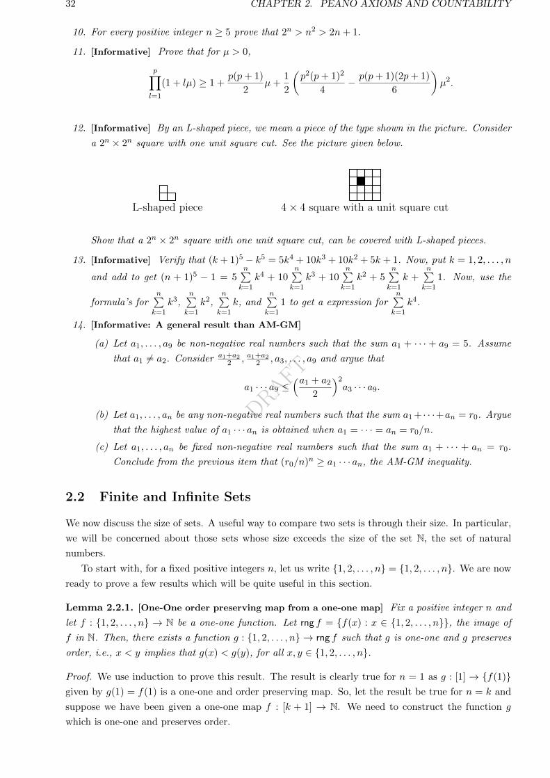
12. [Informative] By an L-shaped piece, we mean a piece of the type shown in the picture. Consider

a 2n × 2n square with one unit square cut. See the picture given below.

L-shaped piece 4 × 4 square with a unit square cut

1

Show that a 2n × 2n square with one unit square cut, can be covered with L-shaped pieces.

13. [Informative] Verify that (k + 1)5 − k5 = 5k4 + 10k3 + 10k2 + 5k + 1. Now, put k = 1, 2, . . . , n

and add to get (n + 1)5 − 1 = 5n∑k=1

k4 + 10n∑k=1

k3 + 10n∑k=1

k2 + 5n∑k=1

k +n∑k=1

1. Now, use the

formula’s forn∑k=1

k3,n∑k=1

k2,n∑k=1

k, andn∑k=1

1 to get a expression forn∑k=1

k4.

14. [Informative: A general result than AM-GM]

(a) Let a1, . . . , a9 be non-negative real numbers such that the sum a1 + · · · + a9 = 5. Assume

that a1 6= a2. Consider a1+a22 , a1+a22 , a3, . . . , a9 and argue that

a1 · · · a9 ≤(a1 + a2

2

)2a3 · · · a9.

(b) Let a1, . . . , an be any non-negative real numbers such that the sum a1 + · · ·+an = r0. Argue

that the highest value of a1 · · · an is obtained when a1 = · · · = an = r0/n.

(c) Let a1, . . . , an be fixed non-negative real numbers such that the sum a1 + · · · + an = r0.

Conclude from the previous item that (r0/n)n ≥ a1 · · · an, the AM-GM inequality.

2.2 Finite and Infinite Sets

We now discuss the size of sets. A useful way to compare two sets is through their size. In particular,

we will be concerned about those sets whose size exceeds the size of the set N, the set of natural

numbers.

To start with, for a fixed positive integers n, let us write 1, 2, . . . , n = 1, 2, . . . , n. We are now

ready to prove a few results which will be quite useful in this section.

Lemma 2.2.1. [One-One order preserving map from a one-one map] Fix a positive integer n and

let f : 1, 2, . . . , n → N be a one-one function. Let rng f = f(x) : x ∈ 1, 2, . . . , n, the image of

f in N. Then, there exists a function g : 1, 2, . . . , n → rng f such that g is one-one and g preserves

order, i.e., x < y implies that g(x) < g(y), for all x, y ∈ 1, 2, . . . , n.

Proof. We use induction to prove this result. The result is clearly true for n = 1 as g : [1] → f(1)given by g(1) = f(1) is a one-one and order preserving map. So, let the result be true for n = k and

suppose we have been given a one-one map f : [k + 1] → N. We need to construct the function g

which is one-one and preserves order.

DRAFT

2.2. FINITE AND INFINITE SETS 33

As rng f is a non-empty subset of N, by the well-ordering principle, rng f contains a least element,

say α ∈ N such that f(x) = α, for some x ∈ [k + 1]. Now, define h : 1, 2, . . . , k → rng f \ α by

h(y) =

f(y) if y < x

f(y + 1) if y ≥ x.

Then, h is one-one as f is one-one and by definition, h is onto. But, by induction step, there exists a

map g1 : 1, 2, . . . , k → rng h = rng f \ α such that g1 is one-one and order preserving. Thus, the

required map g : [k + 1]→ rng f is given by

g(y) =

α if y = 1

g1(y − 1) if y ≥ 2.

Verify that g is indeed one-one and order preserving and hence the required result follows.

As an application of Lemma 2.2.1, we prove the following result.

Lemma 2.2.2. [Injection] Let f : [m] → 1, 2, . . . , n be a one-one function for some m,n ∈ N.

Then m ≤ n.

Proof. As 1, 2, . . . , n ⊆ N, by Lemma 2.2.1 there exists a function g : [m] → rng f ⊆ 1, 2, . . . , nwhich is one-one and order preserving. We claim that g(x) ≥ x, for all x ∈ [m].

Suppose the claim is false. Then, the set S = ` ∈ [m] : g(`) < ` is non-empty subset of N. Hence

by the well ordering principle, S contains a least element, say k ∈ [m] such that g(k) < k. Clearly

k 6= 1 as g(1) ≥ 1. So, we see that g(k−1) ≥ k−1 and g(k) < k. But, g is order preserving and hence

g(k) > g(k − 1) ≥ k − 1,

a contradiction to g(k) < k. Thus, the claim is true.

As g is order preserving and g(x) ∈ 1, 2, . . . , n, one has n ≥ g(m) ≥ m. Thus, n ≥ m and hence

the required result follows.

As an immediate corollary one has the following result. The proof is left for the reader.

Lemma 2.2.3. [Bijection] Let f : [m]→ 1, 2, . . . , n be a bijection for some m,n ∈ N. Then m = n.

The following remark helps us to define cardinality of a finite set.

Remark 2.2.4. [Cardinality of a finite set] Let X be a finite set and suppose there exist m,n ∈ N and

bijections f : [m]→ X and g : 1, 2, . . . , n → X. As g is a bijection, g−1 : X → 1, 2, . . . , n is also a

bijection and hence the map g−1 f : [m]→ 1, 2, . . . , n is a bijection. Thus, by Lemma 2.2.3 m = n.

Thus we see that if X is a finite set then the number m for which there is a bijection f : [m]→ X is

unique. This number m is called the cardinality of X and is generally denoted by |X|. Hence, for

any positive integer m, |[m]| = m.

We now assemble a few important facts on cardinality.

Fact 2.2.5. 1. Let X and Y be two disjoint sets and let f : X → 1, 2, . . . , n and g : Y → [m] be

two bijections. Then, the function h : X ∪ Y → [m+ n] defined by

h(x) =

f(x) if x ∈ Xg(x) + n if x ∈ Y

is a bijection.

DRAFT


2. Fix n ≥ 2 and let f : X → 1, 2, . . . , n be a bijection such that for a fixed element a ∈ X, one

has f(a) = k. Then g : X \ a → 1, 2, . . . , n− 1, defined by

g(x) =

f(x) if f(x) ≤ k − 1

f(x)− 1 if f(x) ≥ k + 1

is a bijection.

3. For any positive integer n and k, there is no bijection from 1, 2, . . . , n to [n+ k].

Proof. Use Lemma 2.2.3.

4. Any subset of 1, 2, . . . , n is finite.

Proof. We use PMI to prove this. It is true for n = 1. Let the result be true for 1, 2, . . . , n−1,.Now, let S ⊆ 1, 2, . . . , n. If n 6∈ S, then S ⊆ 1, 2, . . . , n− 1, and hence using PMI the result

follows. If n ∈ S, let T = S \ n. Then by PMI, T is finite, and hence by Fact 2.2.5.1, S is

finite as S is disjoint union of T and n.

5. Any subset of a finite set is finite.

Proof. Let |S| = n, for some n ∈ N. Then, there is a bijection f : S → 1, 2, . . . , n. Let T ⊆ S.

If T is empty then there is nothing to prove. Else, consider the map fT : T → f(T ). This map

is a bijection. By Fact 2.2.5.4, f(T ) ⊆ 1, 2, . . . , n is finite. Hence, Lemma 2.2.3 gives T is

finite.

6. The set N is not finite.

Proof. Assume that the set N is finite and |N| = n, for some natural number n. But,

1, 2, . . . , n, n + 1 ⊆ N and therefore the identity map Id : 1, 2, . . . , n, n + 1 → N is one-

one. Thus, by Lemma 2.2.2, n+ 1 = |1, 2, . . . , n, n+ 1| ≤ n, a contradiction.

Exercise 2.2.6. 1. Let X and Y be two disjoint sets with |X| = m and |Y | = n. Then |X ∪ Y | =m+ n.

2. Let X be a nonempty finite set and let Y ⊆ X. Then |Y | ≤ |X|. In particular, if Y ( X then

|Y | < |X|.3. Let X be a finite nonempty set and α be a fixed symbol. Now, consider the set Y = (α, a) | a ∈

X. Then |X| = |Y |.4. Let X be a nonempty finite set. Then, for any set Y , |X| = |X \ Y |+ |X ∩ Y |.5. Let X and Y be two finite sets then |X ∪ Y | = |X|+ |Y | − |X ∩ Y |.

Proof. We know X ∪ Y = (X \ Y ) ∪ (X ∩ Y ) ∪ (Y \X). As the sets X \ Y , X ∩ Y , and Y \Xare finite and pairwise disjoint, the result follows from Exercise 2.2.6.1.

To proceed with the next definition, recall that the sets X and Y are said to be equivalent if there

exists a bijection between X and Y .

Definition 2.2.7. [Finite/Countably finite and Infinite/Countably infinite sets]

1. A set X is said to be finite or countably finite if either X is empty or X is equivalent to [m],

for some m ∈ N. A set which is not finite is called an infinite set.

DRAFT

2.3. COUNTABLE AND UNCOUNTABLE SETS 35

2. A set which is either finite or is equivalent to N is called a countable set. In particular, a set

which is equivalent to N is called a countably infinite set.

We now give a few useful criteria to determine whether a set is finite or infinite.

Fact 2.2.8. 1. Let X be an infinite set and Y be a finite set. Then X \ Y is also infinite. In

particular, if a ∈ X, then X \ a is also infinite.

2. A set X is infinite if and only if there is a one-one function f : N→ X.

Proof. Let X be infinite. So X 6= ∅. Let a1 ∈ X. Put f(1) = a1 and X1 = X \ a1. By

Fact 2.2.8.1, X1 is infinite. Assume that we have defined f(1), . . . , f(k) and obtained Xk =

Xk−1 \ ak. As Xk−1 was infinite, by Fact 2.2.8.1, Xk is also infinite. Hence Xk 6= ∅. Let

ak+1 ∈ Xk. Define f(k + 1) = ak+1 and Xk+1 = Xk \ ak+1. By applying induction, f gets

defined on N. Notice that by construction ak+1 /∈ a1, . . . , ak. Hence f is one-one.

Conversely, let f : N→ X be one-one. Then f : N→ f(N) is a bijection. Thus, N is equivalent

to f(N). So, X contains f(N), a countably infinite set. Thus, using Fact 2.2.5.5, X is infinite as

well.

3. A set is infinite if and only if it is equivalent to a proper subset of itself.

Proof. Let S be an infinite set. Then, by Fact 2.2.8.2, there is a one-one function f : N → S.

Now define a map g : S → S \ f(1) by

g(x) =

x, if x 6∈ f(N)

f(k + 1), if x = f(k).

Then, g is indeed a bijection. Thus, S is equivalent to its proper subset S \ f(1).Conversely, let T be a proper subset of a set S such that S and T are equivalent. Suppose S

is finite. Then, by Fact 2.2.5.5, T is finite with |T | < |S|. But, by Remark 2.2.4 |S| = |T |, a

contradiction.

Exercise 2.2.9. 1. Let X be a infinite set and let Y ⊇ X. Then Y is also infinite.

2. Define f : N→ Z by

f(x) =

−x2 if x is evenx−12 if x is odd

.

Prove that f gives an equivalence between N and Z. Thus, Z is countably infinite set.

2.3 Countable and Uncountable sets

In the previous section we learnt that N is a countably infinite set. We now show that the set N× Nis also countably infinite.

Lemma 2.3.1. The set N× N is countably infinite.

Proof. Verify that N × N is equivalent to the set A = (x, y) ∈ N × N : y ≤ x by using the map

g : N × N → A defined by g(x, y) = (x + y − 1, y). Further, use he map f : A → N defined by

f(x, y) =x(x− 1)

2+ y to show that A is equivalent to N.

We now present another proof using the even and odd numbers. Note that this idea can be suitably

generalized to replace 2 by any prime number.

DRAFT


Alternate. Define a map h : N × N → N by h(x, y) = 2x−1(2y − 1). Then, h is one-one as

h(x, y) = h(m,n) if and only if 2x−1(2y − 1) = 2m−1(2n − 1). Now, if x = m then 2y − 1 = 2n − 1

and hence y = n. Therefore (x, y) = (m,n). If x > m then 2x−m(2y − 1) = 2n− 1, a contradiction as

the left hand side is an even number whereas the right hand side is an odd number.

h is onto as every x ∈ N can be uniquely written as x = 2r−1(2n− 1), for some r, n ≥ 1.

Exercise 2.3.2. Let Q+ =mn

: m,n ∈ N, gcd(m,n) = 1

and Q− = −x : x ∈ Q+.

1. Then prove that Q+ is countably infinite.

2. Thus conclude that Q− is countably infinite as well.

3. Therefore, prove that Q is countably infinite.

2.3.1 Cantor’s Lemma

To proceed further, we present Cantor’s experiment. To do so, recall that for any set X, P(X) denotes

the power set of X, i.e., P(X) is the set containing all subsets of X.

Cantor’s Experiment for the student: Why does it happen?

Take a plain paper.

1. On the left draw an oval (of vertical length) and write the elements of 1, 2, 3, 4 inside it,

one below the other. On the right draw a similar but large oval and write the elements of

P(1, 2, 3, 4) inside it, one below the other.

2. Now draw a directed line from 1 (on the left) to any element on the right. Repeat this for

2, 3 and 4. We have drawn a function. Call it f .

3. Notice that f(1), f(2), f(3) and f(4) are sets. Find out the set X = i : i /∈ f(i). Locate

this set on the right.

4. It is guaranteed that you do not have a directed line touching X. Why?

Lemma 2.3.3. [Cantor] Let S be a set and f : S → P(S) be a function. Then, there exists A ∈ P(S)

which does not have a pre-image. That is, there is no surjection from S to P(S).

Proof. On the contrary assume that there exists f : S → P(S) such that f is a surjection. Now,

consider the set A = x : x /∈ f(x) ∈ P(S). As f is a surjection, there exists s ∈ S with f(s) = A.

So, A = f(s) = x : x /∈ f(x). We now show that s neither belongs to A nor to A′.

If s ∈ A, then by definition of A, s /∈ f(s) = A. Similarly, if s /∈ A means that s ∈ f(s) = A.

Thus, s /∈ A ∪A′ = S, a contradiction.

Remark 2.3.4. [Uncountable set] Cantor’s Lemma states that one cannot have a bijection between

a set and its power set. So, the sets N and P(N) cannot be equivalent. Thus, the set P(N) is infinite

but cannot be countably infinite. The sets that are not countable are called uncountable sets.

Definition 2.3.5. 1. [Enumeration] Let A be a countably infinite set. Then, by definition, there

is a bijection f : N→ A. So, we can list all the elements of A as f(1), f(2), . . .. This list is called

an enumeration of the elements of A.

2. [Sequence] An infinite sequence of a non-empty set X is a function f : N → X and is

represented by fii∈N = f1, f2, . . ..

DRAFT


Example 2.3.6. 1. Let S be the set of all 0-1-sequences, i.e., S is the collection of all functions

x : N→ 0, 1. Or equivalently,

S =x : x = x1, x2, . . . where for each i ∈ N, xi ∈ 0, 1

.

Define f : S → P(N) as

f(x) = f(x1, x2, . . .

)= n : xn = 1.

Then f is a bijection. Hence, S is uncountable by Cantor’s lemma.

2. Let T = x ∈ (0, 1) | x has a decimal expansion containing the digits 0 and 1 only. Then T is

uncountable.

Proof. One proof follows by the previous idea.

Alternate. [Cantor’s diagonalization] If T is countably infinite, let x1, x2, · · · be an enumer-

ation of T . Let xn = .xn1xn2 · · · , where xni ∈ 0, 1. Put ynn = 1, if xnn = 0 and ynn = 0,

otherwise. Consider the number y = .y11y22 · · · ∈ T . Notice that for each n, y 6= xn. That is,

y ∈ T but it is not in the enumeration list. This is a contradiction.

2.3.2 Creating Bijections

Experiment 1:

Make a horizontal list of the elements of N using ‘· · · ’ only once. Now, horizontally list the

elements of Z just below the list of N using ‘· · · ’ once. Draw vertical lines to supply a bijection

from N to Z. Can you supply another by changing the second list a little bit?

Experiment 2:

Suppose that you have an open interval (a, b). Its center is c = a+b2 and the distance of the center

from one end is l2 = b−a

2 . View this as a line segment on the real line. Stretch (a, b) uniformly

without disturbing the center and make its length equal to L.

Where is c now (in R)? Where is c − l2? Where is c + l

2? Where is c − α × l2 , for a fixed

α ∈ (−1, 1)?

Now, use the above idea to find a bijection from (a, b) to (s, t)? [Hint: Fix the center first.]

Exercise 2.3.7. 1. Supply two bijections from (1,∞) to (5,∞), one by ‘scaling’ and the other by

‘translating’.

2. Take reciprocal to supply a bijection from (0, 1) to (1,∞). You can also use the exponential

function to get this.

3. Supply a bijection from (−1, 1) to (−∞,∞).

4. Supply a bijection from (0, 1) to R.

5. Supply a bijection from (0, 1)× (0, 1) to R× R.

DRAFT


Train-Seat argument to find a bijection

Let f : P = (0, 1)→ T = (3, 5) be a bijection. Imagine elements of P as PERSONS and elements

of T as seats in a TRAIN. So, f assign a seat to each person and the train is full.

1. Now suppose a new person 0 is arriving. He wants a seat. To manage it, let us un-seat

two persons 12 ,

13 . So, two seats f(12), f(13) are vacant. But we have 3 persons to take those

seats. Giving each person a seat is not possible.

2. Suppose that we un-seat 12 ,

13 , · · · , 1

30? Can we manage it?

3. Suppose that we un-seat 12 ,

13 , · · · ? Can we manage it now?

4. What do we do if we had two new persons arriving? Fifty new persons arriving? A set

a1, a2, · · · of new persons arriving?

The readers are required to prove the next theorem.

Theorem 2.3.8. Let A be a set containing the set a1, a2, . . . , and let f : A → B be a bijection.

Then, prove that, for any collection

1. c1, . . . , ck of elements that are outside A, the function

h(x) =

f(x) if x ∈ A \ a1, a2, . . .f(ai+k) if x = ai, i ∈ Nf(ai) if x = ci, i = 1, 2, . . . , k.

is a bijection from A ∪ c1, . . . , ck to B.

2. c1, c2, . . . of elements that are outside A, the function

h(x) =

f(x) if x ∈ A \ a1, a2, . . .f(a2n−1) if x = an, n ∈ Nf(a2n) if x = cn, n ∈ N

is a bijection from A ∪ c1, c2, . . . to B.

Exercise 2.3.9. Use Theorem 2.3.8 to give bijections from A to B, where

1. A = [0, 1) and B = (0, 1).

2. A = (0, 1) ∪ 1, 2, 3, 4 and B = (0, 1).

3. (0, 1) ∪ N to (0, 1).

4. A = [0, 1] and B = [0, 1] \ 11 , 13 , 15 , · · · .

5. A = R and B = R \ N.

6. A = (0, 1) and B = R \ N.

7. A = [0, 1] and B = R \ N.

8. A = (0, 1) and B = (1, 2) ∪ (3, 4).

9. A = R \ Z and B = R \ N.

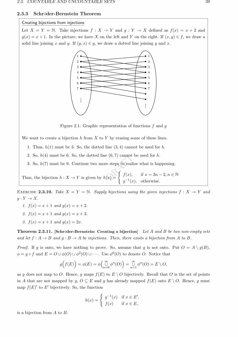
DRAFT


2.3.3 Schroder-Bernstein Theorem

Creating bijections from injections

Let X = Y = N. Take injections f : X → Y and g : Y → X defined as f(x) = x + 2 and

g(x) = x+ 1. In the picture, we have X on the left and Y on the right. If (x, y) ∈ f , we draw a

solid line joining x and y. If (y, x) ∈ g, we draw a dotted line joining y and x.

1

2

3

4

5

6

7

1

2

3

4

5

6

7

... ...

1

Figure 2.1: Graphic representation of functions f and g

We want to create a bijection h from X to Y by erasing some of these lines.

1. Thus, h(1) must be 3. So, the dotted line (3, 4) cannot be used for h.

2. So, h(4) must be 6. So, the dotted line (6, 7) cannot be used for h.

3. So, h(7) must be 9. Continue two more steps to realize what is happening.

Thus, the bijection h : X → Y is given by h(x) =

f(x), if x = 3n− 2, n ∈ Ng−1(x), otherwise.

Exercise 2.3.10. Take X = Y = N. Supply bijections using the given injections f : X → Y and

g : Y → X.

1. f(x) = x+ 1 and g(x) = x+ 2.

2. f(x) = x+ 1 and g(x) = x+ 3.

3. f(x) = x+ 1 and g(x) = 2x.

Theorem 2.3.11. [Schroder-Bernstein: Creating a bijection] Let A and B be two non-empty sets

and let f : A→ B and g : B → A be injections. Then, there exists a bijection from A to B.

Proof. If g is onto, we have nothing to prove. So, assume that g is not onto. Put O = A \ g(B),

φ = g f and E = O ∪ φ(O) ∪ φ2(O) ∪ · · · . Use φ0(O) to denote O. Notice that

g(f(E)

)= φ(E) = φ

( ∞∪n=0

φn(O))

=∞∪n=1

φn(O) = E \O,

as g does not map to O. Hence, g maps f(E) to E \ O bijectively. Recall that O is the set of points

in A that are not mapped by g, O ⊆ E and g has already mapped f(E) onto E \ O. Hence, g must

map f(E)′ to E′ bijectively. So, the function

h(x) =

g−1(x) if x ∈ E′,f(x) if x ∈ E,

is a bijection from A to B.

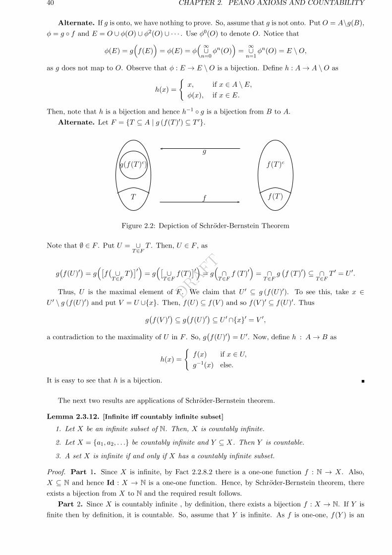
DRAFT


Alternate. If g is onto, we have nothing to prove. So, assume that g is not onto. Put O = A\g(B),

φ = g f and E = O ∪ φ(O) ∪ φ2(O) ∪ · · · . Use φ0(O) to denote O. Notice that

φ(E) = g(f(E)

)= φ(E) = φ

( ∞∪n=0

φn(O))

=∞∪n=1

φn(O) = E \O,

as g does not map to O. Observe that φ : E → E \O is a bijection. Define h : A→ A \O as

h(x) =

x, if x ∈ A \ E,φ(x), if x ∈ E.

Then, note that h is a bijection and hence h−1 g is a bijection from B to A.

Alternate. Let F = T ⊆ A | g (f(T )′) ⊆ T ′.

T f(T )

g(f(T )c) f(T )c

f

g

Figure 2.2: Depiction of Schroder-Bernstein Theorem

Note that ∅ ∈ F . Put U = ∪T∈F

T . Then, U ∈ F , as

g(f(U)′

)= g([f(∪T∈F

T)]′)

= g([∪T∈F

f(T )]′)

= g(∩T∈F

f (T )′)

= ∩T∈F

g(f (T )′

)⊆ ∩

T∈FT ′ = U ′.

Thus, U is the maximal element of F . We claim that U ′ ⊆ g (f(U)′). To see this, take x ∈U ′ \ g (f(U)′) and put V = U ∪x. Then, f(U) ⊆ f(V ) and so f(V )′ ⊆ f(U)′. Thus

g(f(V )′

)⊆ g(f(U)′

)⊆ U ′ ∩x′ = V ′,

a contradiction to the maximality of U in F . So, g(f(U)′

)= U ′. Now, define h : A→ B as

h(x) =

f(x) if x ∈ U,g−1(x) else.

It is easy to see that h is a bijection.

The next two results are applications of Schroder-Bernstein theorem.

Lemma 2.3.12. [Infinite iff countably infinite subset]

1. Let X be an infinite subset of N. Then, X is countably infinite.

2. Let X = a1, a2, . . . be countably infinite and Y ⊆ X. Then Y is countable.

3. A set X is infinite if and only if X has a countably infinite subset.

Proof. Part 1. Since X is infinite, by Fact 2.2.8.2 there is a one-one function f : N → X. Also,

X ⊆ N and hence Id : X → N is a one-one function. Hence, by Schroder-Bernstein theorem, there

exists a bijection from X to N and the required result follows.

Part 2. Since X is countably infinite , by definition, there exists a bijection f : X → N. If Y is

finite then by definition, it is countable. So, assume that Y is infinite. As f is one-one, f(Y ) is an

DRAFT


infinite subset of N and hence by the first part, f(Y ) is countably infinite. So, let g : f(Y )→ N be a

bijection. Then the map g f gives a bijection from Y to N and hence the required result follows.

Part 3. Since X is infinite, by Fact 2.2.8.2 there is a one-one function f : N → X. Thus, f(N)

is a countably infinite subset of X. Conversely, assume that X is finite. Then, by Fact 2.2.5.5, every

subset of X is finite, a contradiction to the assumption that X has a countably infinite subset. Thus,


As a corollary, we have the following result.

Corollary 2.3.13. Let X be uncountable and X ⊆ Y . Then Y is uncountable.

Proof. If Y is countable, then by Lemma 2.3.12, X must be countable, a contradiction.

Theorem 2.3.14. [Power set and uncountability] If S is infinite, then P(S) is uncountable.

Proof. As S is infinite, by Fact 2.2.8.2, there is a one-one map, say f : N → S. Now, define a map

g : P(N)→ P(S) as g(A) = f(A), for all A ∈ P(N). Then, g is clearly one-one and hence g(P(N)

)is

uncountable (as P(N) is uncountable). Hence P(S), being a superset of g(P(N)

), is uncountable, by

Corollary 2.3.13.

Theorem 2.3.15. [Countable union of countable sets] Countable union of countable sets (union of

a countable class of countable sets) is countable.

Proof. Let Aii∈N be a countable class of countable sets and put X = ∪iAi. If X is finite then we

are done. So, let X be infinite. Hence, by Fact 2.2.8.2, there is a one-one map f : N → X. Define

g : X → N as g(x) = 2i3k, if i is the smallest positive integer for which x ∈ Ai and x appears at the

k-th position in the enumeration of Ai. Then g is one-one. Now, by Schroder-Bernstein theorem A is

equivalent to N.

Theorem 2.3.16. [Powet set of N equivalent to R] The set P(N) is equivalent to [0, 1). Furthermore,

P(N) is equivalent to R.

Proof. We already know a one-one map f : P(N) → [0, 1) (see Examples 2.3.6.1 and 2.3.6.2). Let

r ∈ (0, 1). Consider the nonterminating binary representation of r. Denote by Fr the set of positions

of 1 in this representation. Now, define g : [0, 1)→ P(N) by g(r) = Fr, if r 6= 0 and g(0) = ∅. Then g

is one-one. Now, by Schroder-Bernstein theorem P(N) is equivalent to [0, 1).

The next statement follows as [0, 1) is equivalent to (0, 1) (see Exercise 2.3.17.5) and (0, 1) is

equivalent to R.

Exercise 2.3.17. 1. Give a one-one function from N to Q. Define f from Q to N as

f(x) =

2r3s if x = r

s , gcd(r, s) = 1, r > 0, s > 0,

5r3s if x = −rs , gcd(r, s) = 1, r > 0, s > 0,

1 if x = 0

Argue that f is one-one. Apply Schroder-Bernstein theorem to prove that Q is equivalent to N.

2. Give a one-one map from (0, 1) → (0, 1) × (0, 1). For each x ∈ (0, 1), let .x1x2 · · · be the

nonterminating decimal representations1 of x. For x = .x1x2x3 · · · , y = .y1y2y3 · · · , define

f(x, y) = .x1y1x2y2x3y3 · · · . Argue that f is an injection from (0, 1) × (0, 1) to (0, 1). Hence,

show that (0, 1) is equivalent to (0, 1)× (0, 1). Hence, show that R× R is equivalent to R.

1Recall that every real number has a unique nonterminating decimal representation.

DRAFT


3. Fix k ∈ N. Supply a one-one map from N to Nk, the k-fold cartesian product of N. Now, use k

distinct primes to supply a one-one map from Nk to N. Hence, conclude that Nk is equivalent to

N.

4. Supply a bijection from (0, 1) to (1, 2) ∪ (3, 4) ∪ (5, 6) ∪ (7, 8) ∪ · · · .5. Show using Schroder-Bernstein that (0, 1) is equivalent to (0, 1].

6. Let X be a set such that f : N→ X is an onto function. Then, either X is a finite set or X is

countably infinite.

7. Let X = a1, a2, . . . be a countably infinite set and let Y ⊆ X. Then, Y is countable.

8. [Cardinal numbers in brief]

(a) Cardinal numbers are symbols which are associated with sets such that equivalent sets

get the same symbol. By A we denote the cardinal number associated with A.i. If there is an injection f : A → B, then we write A ≤ B. By A ≥ B, we mean that

B ≤ A.

ii. If there is a bijection f : A→ B, then we write A = B.

iii. We write 1, 2, . . . , n as n and ∅ as 0. Thus, for a finite set A, we have A = |A|.iv. We use ℵ0 to denote N. If x = A is a cardinal number by 2x we mean P(A).

(b) Facts about cardinal numbers:i. If x, y, z are cardinal numbers such that x ≤ y and y ≤ z, then x ≤ z. In other words

it says, if there is a one-one map from A to B and a one-one map from B to C, then

there is a one-one map from A to C.

ii. Let x be any cardinal number. Then x 2x. This is Cantor’s lemma.

iii. The cardinal numbers we know till now are 0, 1, 2, 3, . . . ,ℵ0 = N, 2ℵ0 = R, 22ℵ0 , . . ..iv. The cardinal numbers ℵ0 = N, 2ℵ0 = R, 22ℵ0 , . . . are called the infinite cardinal num-

bers.

v. The ‘generalized continuum hypothesis’ says that there is no cardinal number between

an infinite cardinal number x and 2x.

9. Let A be the set of all infinite sequences formed using 0, 1 and B be the set of all infinite sequences

formed using 0, 1, 2. Which one has larger cardinality and why?

10. Write R as a union of pairwise disjoint sets of size 5.

11. Let S be a countable set of points on the unit circle in R2. Consider the line segments Ls with

one end at the origin and the other end at a point s ∈ S. Fix these lines. We are allowed to

rotate the circle anticlockwise (the lines do not move). Let T be another countable set of points

on the unit circle. Can we rotate the circle by an angle θ so that no line Ls touches any of the

points of T?

12. A complex number is algebraic if it is a root of a polynomial equation with integer coefficients.

All other numbers are transcendental. Show that the set of algebraic numbers is countable.

13. Give a bijection from R to R \Q.

2.4 Integers and Modular Arithmetic

In this section, we study some properties of integers. We start with the ‘division algorithm’.

Lemma 2.4.1. [Division algorithm] Let a and b be two integers with b > 0. Then there exist unique

integers q, r such that a = qb + r, where 0 ≤ r < b. The integer q is called the quotient and r, the

remainder.

DRAFT

2.4. INTEGERS AND MODULAR ARITHMETIC 43

Proof. Existence: Take S = a+ bx | x ∈ Z ∩N0. Then a+ |a|b ∈ S. Hence, S is a nonempty subset

of N0. Therefore, by Well-Ordering Principle, S contains its minimum, say s0. So, s0 = a + bx0, for

some x0 ∈ Z. Notice that s0 ≥ 0. We claim that s0 < b.

If s0 ≥ b then s0 − b ≥ 0 and hence s0 − b = a + b(x0 − 1) ∈ S, a contradiction to s0 being the

minimum element of S. Put q = −x0 and r = s0. Thus, we have obtained q and r such that a = qb+r

with 0 ≤ r < b.

Uniqueness: Assume that there exist integers q1, q2, r1 and r2 satisfying a = q1b+ r1, 0 ≤ r1 < b,

a = q2b + r2, and 0 ≤ r2 < b. Without loss of generality, we assume r1 ≤ r2. Then, 0 ≤ r2 − r1 < b.

Notice that r2 − r1 = (q1 − q2)b. So, 0 ≤ (q1 − q2)b < b. But the only integer multiple of b which lies

in [0, b) is 0. Hence, q1 − q2 = 0. Thus, r1 = r2 as well. This completes the proof.

Definition 2.4.2. [Divisibility]

1. [Divisor] Let a, b ∈ Z with b 6= 0. If a = bc, for some c ∈ Z then b is said to divide (be a

divisor of) a and is denoted b | a.

Discussion: If a is a nonzero integer then the set of positive divisors of a is always nonempty

(as 1 | a) and finite (as a positive divisor of a is less than or equal to |a|).

2. [Greatest common divisor/Highest common factor] Let a and b be two nonzero integers.

Then the set S of their common positive divisors is nonempty and finite. Thus, S contains

its greatest element. This element is called the greatest common divisor of a and b and is

denoted gcd(a, b). In some books, the gcd is also called the highest common factor.

3. [Relatively prime/Co-prime integers] An integer a is said to be relatively prime to an

integer b if gcd(a, b) = 1. Or, two integers a and b are said to be co-prime if gcd(a, b) = 1.

The next remark follows directly from the definition and the division algorithm.

Remark 2.4.3. Let a, b ∈ Z \ 0 and d = gcd(a, b). Then, for any positive common divisor c of a

and b, one has c | d.

The next result is often stated as ‘the gcd(a, b) is a linear combination of a and b’.

Theorem 2.4.4. [Bezout’s identity] Let a and b be two nonzero integers. Then, there exist integers

x0, y0 such that d = ax0 + by0, where d = gcd(a, b).

Proof. Consider the set S = ax + by | x, y ∈ Z ∩ N. Then, either a ∈ S or −a ∈ S. Thus, S is

a nonempty subset of N. Hence, by Well-ordering principle, S contains its least element, say d. As

d ∈ S, we have d = ax0 + by0, for some x0, y0 ∈ Z. We claim that d = gcd(a, b).

Note that d is positive. Let c be any positive common divisor of a and b. Then c | ax0 + by0 = d

as x0, y0 ∈ Z. We now show that d | a and d | b.By division algorithm, there exist integers q and r such that a = dq+ r, with 0 ≤ r < d. Thus, we

need to show that r = 0.

On the contrary, assume that r > 0. Then

r = a− dq = a− q(ax0 + by0) = a(1− qx0) + b(−qy0) ∈ ax+ by | x, y ∈ Z.

Hence, r is a positive integer in S which is strictly less than d. This contradicts the fact that d is the

least element of S. Thus, r = 0 and hence d|a. Similarly, d|b.

The division algorithm gives us an idea to algorithmically compute the greatest common divisor

of two integers, commonly known as the Euclid’s algorithm.

DRAFT


Discussion 2.4.5. 1. Let a, b ∈ Z \ 0. By division algorithm, a = |b|q + r, for some integers

q, r ∈ Z with 0 ≤ r < |b|. Then,

gcd(a, b) = gcd(a, |b|) = gcd(|b|, r).

To show the second equality, note that r = a − |b|q and hence gcd(a, |b|) | r. Thus, gcd(a, |b|) |gcd(|b|, r). Similarly, gcd(|b|, r) | gcd(a, |b|) as a = |b|q + r.

2. We can now apply the above idea repeatedly to find the greatest common divisor of two given

nonzero integers. This is called the Euclid’s algorithm. For example, to find gcd(155,−275),

we proceed as follows

−275 = (−2) · 155 + 35 (so, gcd(−275, 155) = gcd(155, 35))

155 = 4 · 35 + 15 (so, gcd(155, 35) = gcd(35, 15))

35 = 2 · 15 + 5 (so, gcd(35, 15) = gcd(15, 5))

15 = 3 · 5 (so, gcd(15, 5) = 5).

To write 5 = gcd(155,−275) in the form 155x0 + (−275)y0, notice that

5 = 35−2·15 = 35−2(155−4·35) = 9·35−2·155 = 9(−275+2·155)−2·155 = 9·(−275)+16·155.

Also, note that 275 = 5 · 55 and 155 = 5 · 31 and thus, 5 = (9 + 31x) · (−275) + (16 + 55x) · 155,

for all x ∈ Z. Therefore, we see that there are infinite number of choices for the pair (x, y) ∈ Z2,

for which d = ax+ by.

3. [Euclid’s algorithm] In general, given two nonzero integers a and b, the algorithm proceeds as

follows:

a = bq0 + r0 with 0 ≤ r0 < b, b = r0q1 + r1 with 0 ≤ r1 < r0,

r0 = r1q2 + r2 with 0 ≤ r2 < r1, r1 = r2q3 + r3 with 0 ≤ r3 < r2,... =

...

r`−1 = r`q`+1 + r`+1 with 0 ≤ r`+1 < r`, r` = r`+1q`+2.

The process will take at most b − 1 steps as 0 ≤ r0 < b. Also, note that gcd(a, b) = r`+1 and

r`+1 can be recursively obtained, using backtracking. That is,

r`+1 = r`−1 − r`q`+1 = r`−1 − q`+1 (r`−2 − r`−1q`) = r`−1 (1 + q`+1q`)− q`+1r`−2 = · · · .

Exercise 2.4.6. 1. Let a, b ∈ N with gcd(a, b) = d. Then gcd(ad ,bd) = 1.

2. Prove that the system 15x+ 12y = b has a solution for x, y ∈ Z if and only if 3 divides b.

3. [Linear Diophantine Equation] Let a, b, c ∈ Z \ 0. Then the linear system ax + by = c, in

the unknowns x, y ∈ Z has a solution if and only if gcd(a, b) divides c. Furthermore, determine

all pairs (x, y) ∈ Z× Z such that ax+ by is indeed c.

4. Prove that gcd(a, bc) = 1 if and only if gcd(a, b) = 1 and gcd(a, c) = 1, for any three nonzero

integers a, b and c.

5. Euclid’s algorithm can sometimes be applied to check whether two numbers which are functions

of an unknown integer n, are relatively prime or not? For example, we can use the algorithm to

prove that gcd(2n+ 3, 5n+ 7) = 1 for every n ∈ Z.

DRAFT


6. [Informative] Suppose a milkman has only 3 cans of sizes 7, 9 and 16 liters. What is the

minimum number of operations required to deliver 1 liter of milk to a customer? Explain.

To proceed further, we need the following definitions.

Definition 2.4.7. [Prime/Composite numbers]

1. [Unity] The positive integer 1 is called the unity (or the unit element) of Z.

2. [Prime] A positive integer p is said to be a prime, if p has exactly two positive divisors, namely,

1 and p.

3. [Composite] A positive integer r is called composite if r 6= 1 and is not a prime.

We are now ready to prove an important result that helps us in proving the fundamental theorem

of arithmetic.

Lemma 2.4.8. [Euclid’s lemma] Let p be a prime and let a, b ∈ Z. If p | ab then either p | a or

p | b.

Proof. If p | a, we are done. So, assume that p - a. As p is a prime, gcd(p, a) = 1. Thus, we can find

integers x, y such that 1 = ax+ py. As p | ab, we have

p | abx+ pby = b(ax+ py) = b · 1 = b.

Thus, if p|ab then either p|a or p|b.

One also has the following result.

Corollary 2.4.9. Let n be an integer such that n | ab and gcd(n, a) = 1. Then n | b.

Proof. As gcd(n, a) = 1, there exists x0, y0 ∈ Z such that nx0 + ay0 = 1. Hence, b = aby0 + nbx0. As

n divides ab, n divides aby0 + n(bx0) = b. Thus, the required result follows.

Now, we are ready to prove the fundamental theorem of arithmetic that states that ‘every positive

integer greater than 1 is either a prime or is a product of primes. This product is unique, except for

the order in which the prime factors appear’.

Theorem 2.4.10. [Fundamental theorem of arithmetic] Let n ∈ N with n ≥ 2. Then there exist

prime numbers p1 > p2 > · · · > pk and positive integers s1, s2, . . . , sk such that n = ps11 ps22 · · · pskk , for

some k ≥ 1. Moreover, if n also equals qt11 qt22 · · · qt`` , for distinct primes q1 > q2 > · · · > q` and positive

integers t1, t2, . . . , t` then k = ` and for each i, 1 ≤ i ≤ k, pi = qi and si = ti.

Proof. We prove the result using the strong form of the principle of mathematical induction. The

result is clearly true for n = 2. So, let the result be true for all m, 2 ≤ m ≤ n − 1. If n is a prime,

then we have nothing to prove. Else, n has a prime divisor p. Then apply induction on np to get the

required result.

Theorem 2.4.11. [Euclid: Infinitude of primes] The number of primes is infinite.

Proof. On the contrary assume that the number of primes is finite, say p1 = 2, p2 = 3, . . . , pk. Now,

consider the positive integer N = p1p2 · · · pk + 1. Then, we see that none of the primes p1, p2, . . . , pk

divides N which contradicts Theorem 2.4.10. Thus, the result follows.

DRAFT


Proposition 2.4.12. [Primality testing] Let n ∈ N with n ≥ 2. Suppose that for any prime p ≤ √n,

p does not divide n then, n is prime.

Proof. Suppose n = xy, for 2 ≤ x, y < n. Then, either x ≤ √n or y ≤ √n. Without loss of generality,

assume x ≤ √n. If x is a prime, we are done. Else, take a prime divisor of x to get a contradiction.

Exercise 2.4.13. [Informative] Prove that there are infinitely many primes of the form 4n− 1.

Definition 2.4.14. [Least common multiple] Let a, b ∈ Z. Then the least common multiple of

a and b, denoted lcm(a, b), is the smallest positive integer that is a multiple of both a and b.

Theorem 2.4.15. Let a, b ∈ N. Then, gcd(a, b) · lcm(a, b) = ab. Thus, lcm(a, b) = ab if and only if

gcd(a, b) = 1.

Proof. Let d = gcd(a, b). Then d = as + bt, for some s, t ∈ Z, a = a1d, b = b2d, for some a1, b1 ∈ N.

We need to show that lcm(a, b) = a1b1d = ab1 = a1b, which is clearly a multiple of both a and b. Let

c ∈ N be any common multiple of a and b. To show, a1b1d divides c. Note that

c

a1b1d=

cd

(a1d) · (b1d)=c(as+ bt)

ab=c

bs+

c

at ∈ Z

as ca ,

cb ∈ Z and s, t ∈ Z. Thus, a1b1d = lcm(a, b) divides c and hence lcm(a, b) is indeed the smallest.


Definition 2.4.16. [Modular Arithmetic] Fix a positive integer n. Then, ‘an integer a is said to be

congruent to an integer b modulo n’, denoted a ≡ b (mod n), if n divides a− b.

Example 2.4.17. 1. It can be easily verified that any two even (odd) integers are equivalent

modulo 2 as 2 | 2(l −m) = 2l − 2m (2 | 2(l −m) = ((2l + 1)− (2m+ 1))).

2. The numbers ±10 and 22 are equivalent modulo 4 as 4 | 12 = 22− 10 and 4 | 32 = 22− (−10).

3. Let n be a fixed positive integer and let S = 0, 1, 2, . . . , n− 1.

(a) Then, by division algorithm, for any a ∈ Z there exists a unique b ∈ S such that a ≡ b

(mod n). The number b is called the residue of a modulo n.

(b) Thus, the set of integers, Z =n−1⋃a=0a + kn : k ∈ Z, i.e., every integer is congruent to an

element of S. The set S is taken as the standard representative for the set of residue

classes modulo n.

Theorem 2.4.18. Let n be a positive integer. Then, the following results hold.

1. Let a ≡ b (mod n) and b ≡ c (mod n), for some a, b, c ∈ Z. Then, a ≡ c (mod n).

2. Let a ≡ b (mod n), for some a, b ∈ Z. Then, a ± c ≡ b ± c (mod n) and ac ≡ bc (mod n), for

all c ∈ Z.

3. Let a ≡ b (mod n) and c ≡ d (mod n), for some a, b, c, d ∈ Z. Then, a± c ≡ b± d (mod n) and

ac ≡ bd (mod n). In particular, am ≡ bm (mod n), for all m ∈ N.

4. Let ac ≡ bc (mod n), for some non-zero a, b, c ∈ Z. Then, a ≡ b (mod n), whenever gcd(c, n) =

1. In general, a ≡ b (modn

gcd(c, n)).

DRAFT


Proof. We will only prove two parts. The readers should supply the proof of other parts.

Part 3: Note that ac − bd ≡ ac − bc + bc − bd ≡ c(a − b) + b(c − d). Thus, n | ac − bd, whenever

n | a− b and n | c− d.

In particular, taking c = a and d = b and repeatedly applying the above result, one has am ≡ bm

(mod n), for all m ∈ N.

Part 4: Let gcd(c, n) = d. Then, there exist non-zero c1, n1 ∈ Z and c = c1d, n = n1d. Thus,

n | ac − bc means that n1d | c1d(a − b). This, in turn implies that n1 | c1(a − b). Hence, by

Corollary 2.4.9, we getn

gcd(c, n)= n1 | a− b.

Before coming to the next result, we look at the following examples.

Example 2.4.19. 1. Note that 3 · 9 + 13 · (−2) ≡ 1 (mod 13). So, the system 9x ≡ 4 (mod 13)

has the solution

x ≡ x · 1 ≡ x · (3 · 9 + 13 · (−2)) ≡ 3 · 9x ≡ 3 · 4 ≡ 12 (mod 13).

2. Verify that 9 · (−5) + 23 · (2) = 1. Hence, the system 9x ≡ 1 (mod 23) has the solution

x ≡ x · 1 ≡ x (9 · (−5) + 23 · (2)) ≡ (−5) · (9x) ≡ −5 ≡ 18 (mod 23).

3. The system 3x ≡ 15 (mod 30) has solutions x = 5, 15, 25, whereas the system 7x = 15 has only

the solution x = 15. Also, verify that the system 3x ≡ 5 (mod 30) has no solution.

Theorem 2.4.20. [Linear Congruence] Let n be a positive integer and let a and b be non-zero

integers. Then, the system ax ≡ b (mod n) has at least one solution if and only if gcd(a, n) | b.Moreover, if d = gcd(a, n) then ax ≡ b (mod n) has exactly d solutions in 0, 1, 2, . . . , n− 1.

Proof. Let x0 be a solution of ax ≡ b (mod n). Then, by definition, ax0 − b = nq, for some q ∈ Z.

Thus, b = ax0 − nq. But, gcd(a, n) | a, n and hence gcd(a, n) | ax0 − nq = b.

Suppose d = gcd(a, n) | b. Then, b = b1d, for some b1 ∈ Z. Also, by Euclidean algorithm, there

exists x0, y0 ∈ Z such that ax0 + ny0 = d. Hence,

a(x0b1) ≡ b1(ax0) ≡ b1(ax0 + ny0) ≡ b1d ≡ b (mod n).

This completes the proof of the first part.

To proceed further, assume that x1, x2 are two solutions. Then, ax1 ≡ ax2 (mod n) and hence,

by Theorem 2.4.18.4, x1 ≡ x2 (modn

d). Thus, we can find x2 ∈ 0, 1, . . . ,

n

d such that x = x2 + k

n

dis a solution of ax ≡ b (mod n), for 0 ≤ k ≤ d− 1. Verify that these x’s are distinct and lie between

0 and n− 1. Hence, the required result follows.

Exercise 2.4.21. 1. Prove Theorem 2.4.18.

2. Determine the solutions of the system 3x ≡ 5 (mod 65).

3. Determine the solutions of the system 5x ≡ 95 (mod 100).

4. Prove that the system 3x ≡ 4 (mod 28) is equivalent to the system x ≡ 20 (mod 28).

5. Prove that the pair of systems 3x ≡ 4 (mod 28) and 4x ≡ 2 (mod 27) is equivalent to the pair

x ≡ 20 (mod 28) and x ≡ 14 (mod 27). Hence, prove that the above system is equivalent to

solving either 20 + 28k ≡ 14 (mod 27) or 14 + 27k ≡ 20 (mod 28) for the unknown quantity

k. Thus, verify that k = 21 is the solution for the first case and k = 22 for the other. Hence

x = 20 + 28 · 21 = 608 = 14 + 22 · 27 is a solution of the above pair.

DRAFT


6. Let p be a prime. Then, prove that p |(pk

)=

p!

k!(p− k)!, for 1 ≤ k ≤ p− 1.

7. [Informative] Let p be a prime. Then, the set

(a) Zp = 0, 1, 2, . . . , p− 1 has the following properties:i. for every a, b ∈ Zp, a+ b (mod p) ∈ Zp.

ii. for every a, b ∈ Zp, a+ b = b+ a (mod p).

iii. for every a, b, c ∈ Zp, a+ (b+ c) ≡ (a+ b) + c (mod p).

iv. for every a ∈ Zp, a+ 0 ≡ a (mod p).

v. for every a ∈ Zp, a+ (p− a) ≡ 0 (mod p).

(b) Z∗p = 1, 2, . . . , p− 1 has the following properties:i. for every a, b ∈ Zp, a · b (mod p) ∈ Z∗p.

ii. for every a, b ∈ Z∗p, a · b = b · a (mod p).

iii. for every a, b, c ∈ Z∗p, a · (b · c) ≡ (a · b) · c (mod p).

iv. for every a ∈ Z∗p, a · 1 ≡ a (mod p).

v. for every a ∈ Z∗p, a · b ≡ 1 (mod p). To see this, note that gcd(a, p) = 1. Hence, by

Euclid’s algorithm, there exists x, y ∈ Z such that ax+ py = 1. Define b ≡ x (mod p).

Then,

a · b ≡ a · x ≡ a · x+ p · y ≡ 1 (mod p).

In algebra, any set, say F, in which ‘addition’ and ‘multiplication’ can be defined in such a

way that the above properties are satisfied then F is called a field. So, Zp = 0, 1, 2, . . . , p−1 is an example of a field. In general, the well known examples of fields are:

i. Q, the set of rational numbers.

ii. R, the set of real numbers.

iii. C, the set of complex numbers.

(c) From now on let p be an odd prime.i. Then, the equation x2 ≡ 1 (mod p). Since, p is a prime, the only solutions in Zp are

x = 1, p− 1.

ii. Then, for a ∈ 2, 3, . . . , p− 2, the number b ∈ Z∗p that satisfies a · b ≡ 1 (mod p) also

satisfies b ∈ 2, 3, . . . , p− 2 and b 6= a.

iii. Thus, for 1 ≤ i ≤ p−12 , we have pairs ai, bi that are pairwise disjoint and satisfy

ai · bi ≡ 1 (mod p). Moreover,

p−12⋃i=1ai, bi = 2, 3, . . . , p− 2.

iv. Hence, 2 · 3 · · · · · (p− 2) ≡ 1 (mod p).

v. We thus have the following famous theorem called the Wilson’s Theorem: Let p be a

prime. Then (p− 1)! ≡ −1 (mod p). Proof. Note that from the previous step, we have

(p− 1)! ≡ 1 · (p− 1) · 2 · 3 · · · · · (p− 2) ≡ −1 · 1 ≡ −1 (mod p).

vi. (Primality Testing) Let n be a positive integer. Then, (n − 1)! ≡ −1 (mod n) if and

only if n is a prime.

Theorem 2.4.22. [Chinese remainder theorem] Fix a positive integer m and let n1, n, . . . , nm be

pairwise co-prime positive integers. Then, the linear system

x ≡ a1 (mod n1)

x ≡ a2 (mod n2)...

x ≡ am (mod nm)

DRAFT


has a unique solution modulo M = n1n2 · · ·nm.

Proof. For 1 ≤ k ≤ m, define Mk =M

nk. Then, gcd(Mk, nk) = 1 and hence there exist integers xk, yk

such that Mkxk + nkyk = 1 for 1 ≤ k ≤ m. Then

Mkxk ≡ 1 (mod nk) and Mkxk ≡ 0 (mod n`) for ` 6= k.

Define x0 =m∑k=1

Mkxkak. Then, it can be easily verified that x0 satisfies the required congruence

relations.

Example 2.4.23. Let us come back to Exercise 2.4.21.5. In this case, M = 28 · 27 = 756,M1 = 27

and M2 = 28. Therefore, x1 = −1 and x2 = 1. Thus,

x0 = 27 · −1 · 20 + 28 · 1 · 14 ≡ −540 + 392 ≡ −148 ≡ 608 (mod 756).

Exercise 2.4.24. 1. Find the smallest positive integer which when divided by 4 leaves a remained

1 and when divided by 9 leaves a remainder 2.

2. Find the smallest positive integer which when divided by 8 leaves a remained 4 and when divided

by 15 leaves a remainder 10.

3. Does there exist a positive integer n such that

n ≡ 4 (mod 14), n ≡ 6 (mod 18)?

Give reasons for your answer. What if we replace 6 or 4 with an odd number?

4. [Informative] Let n be a positive integer. Then, the set

(a) Zn = 0, 1, 2, . . . , n− 1 has the following properties:i. for every a, b ∈ Zn, a+ b (mod n) ∈ Zn.

ii. for every a, b ∈ Zn, a+ b = b+ a (mod n).

iii. for every a, b, c ∈ Zn, a+ (b+ c) ≡ (a+ b) + c (mod n).

iv. for every a ∈ Zn, a+ 0 ≡ a (mod n).

v. for every a ∈ Zn, a+ (p− a) ≡ 0 (mod n).

vi. for every a, b ∈ Zn, a · b (mod n) ∈ Zn.

vii. for every a, b ∈ Zn, a · b = b · a (mod n).

viii. for every a, b, c ∈ Zn, a · (b · c) ≡ (a · b) · c (mod n).

ix. for every a ∈ Zn, a · 1 ≡ a (mod n).

In algebra, any set, say R, in which ‘addition’ and ‘multiplication’ can be defined in such

a way that the above properties are satisfied then R is called a commutative ring with

unity. So, Zn = 0, 1, 2, . . . , n − 1 is an example of a commutative ring with unity. In

general, the well known examples of commutative ring with unity are:i. Z, the set of integers.

ii. Q, the set of rational numbers.

iii. R, the set of real numbers.

iv. C, the set of complex numbers.

(b) Now, let m and n be two co-prime positive integers. Then, by the above, the sets Zm,Zn, and

Zmn are commutative rings with unity. In the following, we show that there is a one-to-one

correspondence (ring isomorphism) between Zm × Zn and Zmn. To do so, define

f : Zmn → Zm × Zn by f(x) = (x (mod m), x (mod n)) for all x ∈ Zmn.

Then, defining ‘addition’ and ‘multiplication’ in Zm × Zn component-wise and using Theo-

rem 2.4.18, we have the following:

DRAFT


i. f(x+ y) = f(x) + f(y), for all x, y ∈ Zmn.

ii. f(x · y) = f(x) · f(y), for all x, y ∈ Zmn.

iii. for every (a, b) ∈ Zm × Zn, by CRT, there exists a unique x ∈ Zmn such that

x ≡ a (mod m) and x ≡ b (mod n).

iv. also, | Zm × Zn |=| Zmn |= mn..

Hence, we have obtained the required one-one correspondence, commonly known as the ring

isomorphism. That is, the two rings Zm × Zn and Zmn are isomorphic.

2.5 Construction of Integers and Rationals∗

This section contains two subsections. In the first subsection, we construct integers from natural

numbers and prove a few properties, such as addition, multiplication and subtraction. The second

subsection generalizes the ideas in the first subsection to construct rationals and then study a few

properties of rationals.

2.5.1 Construction of Integers

To start with let X = N× N. We define a relation ‘∼’ on X by

(a, b) ∼ (c, d) if a+ d = b+ c for all a, b, c, d ∈ N.

Then, verify that ∼ is indeed an equivalence relation on X. Let Z denote the collection of all equiv-

alence classes under this relation. So, if [x], [y] ∈ Z then [x] is an equivalence class containing

x = (x1, x2), for some x1, x2 ∈ N and [y] is an equivalence class containing y = (y1, y2), for some

y1, y2 ∈ N. Now, using the successor function S defined in Axiom P2, observe that Z consists of all

equivalence classes of the form

1. [(1, 1)] = (n, n) : for all n ∈ N,2. for a fixed element m ∈ N, [(1, S(m))] = (n,m+ n) : for all n ∈ N, and

3. for a fixed element m ∈ N, [(S(m), 1)] = (m+ n, n) : for all n ∈ N.

Definition 2.5.1. [Addition in Z] Let [x] = [(x1, x2)], [y] = [(y1, y2)] ∈ Z, for some x1, x2, y1, y2 ∈ N.

Then, one defines addition in Z, denoted by ⊕, as

[x]⊕ [y] = (x1, x2)⊕ (y1, y2) = [(x1 + y1, x2 + y2)]. (2.3)

Note that basically we have defined a map ⊕ : Z × Z → Z which takes two non-empty sets, say

[(x1, x2)] and [(y1, y2)] and gives a set [(x1+y1, x2+y2)]“namely the addition of the two” as the image.

Thus, we need to verify that the addition of two different representatives of the domain, give rise to

the same set on the range. This process of defining a map using representatives and then verifying

that the image is independent of the representatives chosen is characterized by saying that “the map

is well-defined”. So, let us now prove that ⊕ is well-defined.

Lemma 2.5.2. The map ⊕ defined in Equation (2.3) is well-defined.

Proof. Let [(u1, u2)] = [(v1, v2)] and [(x1, x2)] = [(y1, y2)] be two equivalence classes in Z. Then, by

definition

[(u1, u2)]⊕ [(x1, x2)] = [(u1 + x1, u2 + x2)] and [(v1, v2)]⊕ [(y1, y2)] = [(v1 + y1, v2 + y2)].

DRAFT

2.5. CONSTRUCTION OF INTEGERS AND RATIONALS∗ 51

For well-definedness, we need to show that [(u1 + x1, u2 + x2)] = [(v1 + y1, v2 + y2)]. Or equivalently,

we need to show that u1 + x1 + v2 + y2 = u2 + x2 + v1 + y1.

But, the equality of the equivalence classes [(u1, u2)] = [(v1, v2)] and [(x1, x2)] = [(y1, y2)] implies

u1 + v2 = u2 + v1 and x1 + y2 = x2 + y1.

Thus, adding the two and using the commutativity of addition in N, we get u1 + x1 + v2 + y2 =

u2 + x2 + v1 + y1. Thus, the required result follows.

In this particular case, one can also check the following statements to verify the well-definedness

of ⊕, i.e., one needs to show that for all `,m, n, r ∈ N the following statements hold.

1. [(1, 1)]⊕ [(n, n)] = [(m,m)] + [(n, n)].

2. [(1, S(m))]⊕ [(1, S(`))] = [(r,m+ r)]⊕ [(n, `+ n)].

3. [(S(m), 1)]⊕ [(S(`), 1)] = [(m+ r, r)]⊕ [(`+ n, n)].

4. [(1, 1)]⊕ [(1, S(m))] = [(n, n)]⊕ [(r,m+ r)] = [(1, 1)]⊕ [(r,m+ r)] = [(r, r)]⊕ [(1, S(m))].

5. [(1, 1)]⊕ [(S(m), 1)] = [(n, n)]⊕ [(m+ r,m)] = [(1, 1)]⊕ [(m+ r,m)] = [(r, r)]⊕ [(S(m), 1)]?.

6. [(1, S(m))]⊕ [(S(`), 1)] = [(r,m+ r)]⊕ [(`+ n, n)] and so on.

We give the argument for the fourth statement. The readers are supposed to provide arguments for

other statements.

1. [(1, 1)]⊕[(1, S(m))] = [(2, S(m)+1)] = [(n+r,m+n+r)] as using commutativity and associativity

of addition of natural numbers, one has

2 +m+ n+ r = m+ 2 + n+ r = (m+ 1) + 1 + n+ r = S(m) + 1 + n+ r.

Hence, [(1, 1)]⊕ [(1, S(m))] = [(n+ r,m+ n+ r)] = [(n, n)]⊕ [(r,m+ r)].

2. [(1, 1)]⊕ [(r,m+ r)] = [(r + 1,m+ r + 1)] = [(r + 1, r + S(m))] = [(r, r)]⊕ [(1, S(m))].

On similar lines, we now define multiplication among elements of Z.

Definition 2.5.3. [Multiplication of Integers] Let [x] = [(x1, x2)], [y] = [(y1, y2)] ∈ Z, for some

x1, x2, y1, y2 ∈ N. Then, one defines multiplication in Z, denoted by , as

[x] [y] = [(x1, x2)] [(y1, y2)] = [(x1y1 + x2y2, x1y2 + x2y1)]. (2.4)

Since we are talking about multiplication between two sets using their representatives, we need

to verify that the multiplication is indeed well-defined. So, the readers are required to prove “well-

definedness” of multiplication. The readers can now prove all the properties of addition and multipli-

cation in Z by using the corresponding properties of natural numbers.

Exercise 2.5.4. Let [x], [y], [z] ∈ Z and let us denote [0] = [(1, 1)]. Then, prove that

1. [Associativity of addition] ([x] + [y]) + [z] = [x] + ([y] + [z]).

2. [Commutativity of addition] [x] + [y] = [y] + [x].

3. [Existence of the zero element] [x] + [0] = [x].

4. [Cancellation property holds] If [x] + [y] = [x] + [z] then [y] = [z]. This implies that the zero

element is unique.

5. [Existence of additive inverse] for every [x] = [(x1, x2)], the equivalence class [(x2, x1)], denoted

by −[x], satisfies [x] ⊕ (−[x]) = [0]. Now, use the cancellation property in Z to show that the

additive inverse is unique.

DRAFT


6. [Distributive laws] ([x] + [y]) [z] = [x] [z]⊕ [y] [z].

7. [Associativity of multiplication] ([x] [y]) [z] = [x] ([y] [z]).

8. [Commutativity of multiplication] [x] [y] = [y] [x].

9. [Existence of the identity element] [x] [1] = [x], where [1] = [(S(1), 1)].

10. [Cancellation property holds] If [x] [y] = [x] [z] with [x] 6= [0] then [y] = [z]. This implies

that the identity element is unique.

11. [x] [0] = [0].

As a last property, we show that a copy of N naturally seats inside Z.

Lemma 2.5.5. Consider the map f : N → Z defined by f(n) = [(S(n), 1)], for all n ∈ N. Then, for

all a, b ∈ N1. f is one-one,

2. f(a+ b) = f(a)⊕ f(b), and

3. f(a · b) = f(a) f(b).

Proof. Part 1.: Suppose f(a) = f(b) for some a, b ∈ N. Then, by definition, [(S(a), 1)] = [(S(b), 1)],

or equivalently, S(a) + 1 = S(b) + 1. Now, use cancellation in N to get S(a) = S(b). Thus, a = b as S

is an injective map.

Part 2.: By definition, f(a+ b) = [(S(a+ b), 1)] and

f(a)⊕ f(b) = [(S(a), 1)]⊕ [(S(b), 1)] = [(S(a) + S(b), 1 + 1)] = [(S(a) + b+ 1, 1 + 1)]

= [(S(a+ b) + 1, 1 + 1)] = [(S(a+ b), 1)] = f(a+ b).

Part 3.: By definition, f(a · b) = [(S(a · b), 1)] and

f(a) f(b) = [(S(a), 1)] [(S(b), 1)] = [(S(a) · S(b) + 1 · 1, S(a) · 1 + 1 · S(b))]

= [(S(a) · S(b) + 1, S(a) + S(b))] = [(S(a · b), 1)] = f(a b)

as S(a) ·S(b) + 1 + 1 = S(a) · b+S(a) · 1 + 1 + 1 = a · b+ 1 · b+S(a) + 1 + 1 = S(a · b) +S(b) +S(a).

Thus, we have indeed shown that N is seating inside Z as f (N) and the addition and multiplication

operations are satisfied by f (the map f commutes with the addition operation and the multiplication

operation). So, from now on, the symbols + and · will be used for addition and multiplication in

integers. Further, as n ∈ N is identified with f(n) = [(S(n), 1)], we would like to associate the symbol

‘−’ as n = S(n)− 1 and −n = 1− S(n). We proceed to do this in the next few paragraphs.

Definition 2.5.6. [Order in Z] Let [x] = [(x1, x2)], [y] = [(y1, y2)] ∈ Z, for some x1, x2, y1, y2 ∈ N.

Then, the order in Z is defined by saying that [x] < [y] if x1 + y2 < y1 + x2. Further, [x] ≤ [y] if

either [x] = [y] or [x] < [y].

We again need to check for well-definedness. So, let [(u1, u2)] = [(v1, v2)] and [(x1, x2)] = [(y1, y2)]

be two equivalence classes in Z with [(u1, u2)] < [(x1, x2)]. We need to show that [(v1, v2)] < [y1, y2)].

Or equivalently, v1 + y2 < y1 + v2 whenever u1 + v2 = v1 +u2, x1 + y2 = y1 +x2 and u1 +x2 < x1 +u2.

Thus,

v1 + y2 + x1 + u2 = v1 + u2 + x1 + y2 = u1 + v2 + y1 + x2 = y1 + v2 + u1 + x2

< y1 + v2 + x1 + u2.

Hence, by the order property in N (see Exercise 2.1.10), v1 + y2 < y1 + v2. Thus, the above definition

is well-defined. At this stage, one would like to verify that the function f defined in Lemma 2.5.5

preserves the order as well.

DRAFT


Lemma 2.5.7. Consider the map f : N → Z defined by f(n) = [(S(n), 1)], for all n ∈ N. Then, for

all a, b ∈ N, a < b if and only if f(a) < f(b).

Proof. Using Exercise 2.1.10 a < b if and only if a + 1 + 1 < b + 1 + 1, or equivalently, a < b if and

only if S(a) + 1 < S(b) + 1. Thus, a < b if and only if f(a) = [(S(a), 1)] < [(S(b), 1)] = f(b).

Definition 2.5.8. [Positive elements in Z] Let [x] = [(x1, x2)] ∈ Z. Then, [x] is said to be positive

if [0] < [x] and is said to be non-negative if [0] ≤ [x]. In general, we write [x] > [0] to mean [x] is

positive and [x] ≥ [0] for [x] being non-negative.

Lemma 2.5.9. Let [x] = [(x1, x2)] ∈ Z. Then, [x] > [0] if and only if x1 > x2.

Proof. By definition, [(x1, x2)] > [0] = [(1, 1)] if and only if x1 + 1 > x2 + 1. Or equivalently, using

Exercise 2.1.10, one obtains [(x1, x2)] > [(1, 1)] if and only if x1 > x2.

Exercise 2.5.10. 1. Prove the following results for any [x] ∈ Z.

(a) [x] > 0 if and only if [x] = [(S(n), 1)] = f(n), for some n ∈ N.

(b) [x] > 0 if and only if −[x] < 0.

2. [y] > [z], for some [y], [z] ∈ Z if and only if [y] + [x] > [z] + [x].

3. If [y] > [z], for some [y], [z] ∈ Z then [y] · [x] > [z] · [x], whenever [x] > 0.

Thus, Z = N∪ 0 ∪ (−N) and hence from now on, in place of using equivalence class to represent

the elements of Z, we will just use natural numbers, their negatives and the zero element to represent

Z, the set of integers. Thus, whenever we define functions or operations on Z then we don’t have to

worry about well-definedness. Let us now discuss the “absolute value function”, namely the modulus

function.

Definition 2.5.11. A function g : Z→ N ∪ 0 is called as absolute/modulus function if

1. g(n) = n if n ≥ 0,

2. g(n) = −n, if n < 0.

This function is denoted by | · |. Thus, |m| = m, if m ≥ 0 and −m, if m < 0. Further, by Exer-

cise 2.5.10.1, observe that |m| ≥ 0 for all m ∈ Z.

For a better understanding of this function, we prove the following two results.

Lemma 2.5.12. For any x ∈ Z, −|x| ≤ x ≤ |x|. Further, if x ≥ 0 and −x ≤ y ≤ x for some y ∈ Zthen |y| ≤ x.

Proof. Let x ≥ 0. Then, by definition |x| = x and hence x ≤ |x|. As |x| = x, the other inequality

−|x| ≤ x reduces to −x ≤ x. Or equivalently, we need to show that 0 = x+ (−x) ≤ x+x = 2x, which

is indeed true. If x < 0 then we see that |x| > 0 > x and hence x ≤ |x|. Note that the condition

−|x| ≤ x is equivalent to the condition |x|+ x ≥ 0 (use Exercise 2.5.10.2) which is indeed true as by

definition x+ |x| = x+ (−x) = 0.

For the second part, we again consider two cases, namely, y ≥ 0 and y < 0. If y ≥ 0 then |y| = y

and hence the condition y ≤ x implies |y| ≤ x. In case y < 0 implies |y| = −y. Further, using

Exercise 2.5.10.2, the condition −x ≤ y is equivalent to the condition 0 ≤ y + x which in turn is

equivalent to −y ≤ x. Hence |y| = −y ≤ x. Thus, the required result follows.

As a direct application of Lemma 2.5.12, one obtains the triangle inequality.

DRAFT


Lemma 2.5.13. [Triangle inequality in Z] Let x, y ∈ Z. Then |x+ y| ≤ |x|+ |y|.

Proof. Using Lemma 2.5.12, one has −|x| ≤ x ≤ |x| and −|y| ≤ y ≤ |y|. Hence,

−|x|+ (−|y|) ≤ x+ y ≤ |x|+ |y|.

Now, use the associativity and commutativity of addition to get

0 = −|x|+ (−|y|) + |x|+ |y| = −(|x|+ |y|) + (|x|+ |y|)

and hence the uniqueness of the additive inverse implies −|x| + (−|y|) = −(|x| + |y|). Thus, the

required result follows from the second part of Lemma 2.5.12.

This finishes most of the results on the basic operations related with integers.

2.5.2 Construction of Rational Numbers

In this subsection, we will describe the construction of rational numbers and prove a few properties,

such as addition, multiplication, subtraction and division by non-zero element.

So, let us start with denoting Z∗ = Z \ 0 and defining an equivalence relation on X = Z × Z∗and then doing everything afresh as was done for the set of integers. Define a relation ‘∼’ on X by

(a, b) ∼ (c, d) if a · d = b · c for all a, c ∈ Z, b, d ∈ Z∗.

Then, verify that ∼ is indeed an equivalence relation on X. Let Q denote the collection of all

equivalence classes under this relation. This set is called the “set of rational numbers”. In this

set, we define addition and multiplication, using the addition and multiplication in Z, as follows:

1. [Addition in Q] Let [x] = [(x1, x2)], [y] = [(y1, y2)] ∈ Q. Then, one defines addition in Q,

denoted by ⊕, as

[x]⊕ [y] = (x1, x2)⊕ (y1, y2) = [(x1 · y2 + x2 · y1, x2 · y2)].

2. [Multiplication in Q] Let [x] = [(x1, x2)], [y] = [(y1, y2)] ∈ Q. Then, one defines multiplication

in Q, denoted by , as

[x] [y] = (x1, x2) (y1, y2) = [(x1 · y1, x2 · y2)].

The readers are advised to verify the well-definedness of the above operations in Q. Further, if we

define the map f : Z → Q by f(a) = [(a, 1)] then it can be easily verified that the map f is one-one

and it preserves addition and multiplication. Thus, Z is seating inside Q as f(Z). So, again one

replaces the symbols ‘⊕’ and ‘’ by ‘+’ and ‘·’. Sometimes, even ‘·’ is not used for multiplication. We

also note that the element 0 ∈ Z corresponds to [(0, 1)] = [(0, x)], for all x ∈ Z∗. Hence, an element

[(x1, x2)] ∈ Q with [(x1, x2)] 6= 0 implies that x1 6= 0. Thus, verify that for each [(x1, x2)] ∈ Q with

x1 6= 0, the element [(x2, x1)] ∈ Q satisfies [(x1, x2)] · [(x2, x1)] = 1. As the next operation, one defines

division in Q as follows.

Definition 2.5.14. [Division in Q] Let [x] = [(x1, x2)], [y] = [(y1, y2)] ∈ Q with y1 6= 0. Then, one

defines division in Q, denoted by /, as

[x]/[y] = [(x1, x2)]/[(y1, y2)] = [(x1y2, x2y1)].

Note that x2y1 ∈ Z∗ as x2, y1 6= 0.

DRAFT


The readers are advised to verify the well-definedness of division defined above. Before proceeding

further with other important properties of rational numbers, the readers should verify all the properties

related with addition, subtract, multiplication and division by a non-zero element. The next result,

even though it doesn’t seem important, helps us to define order in rational numbers.

Lemma 2.5.15. [Representation of an element of Q] Let [x] ∈ Q. Then [x] = [(y1, y2)], for some

y1, y2 ∈ Z such that y2 > 0.

Proof. Let [x] = [(x1, x2)], for some x1, x2 ∈ Z. If x2 > 0, we are done. Else, using Exercise 2.5.10.1,

we know that −x2 > 0. Then, by the definition of equivalence class [x] = [(x1, x2)] = [(−x1,−x2)].Hence, the required result follows.

So, now we proceed with the definition of order in Q.

Definition 2.5.16. [Order in Q] Let [x] = [(x1, x2)], [y] = [(y1, y2)] ∈ Q, for some x1, x2, y1, y2 ∈ Zwith x2, y2 > 0. Then the order in Q is defined by [x] > [y] if x1y2 > x2y1.

We again need to verify the well-definedness of order in Q. Also, as before, [x] ≥ [y] means either

[x] = [y] or [x] > [y]. As a final result of this section, we prove the following result.

Lemma 2.5.17. [Existence of rational between two rational] Let [x], [y] ∈ Q with [x] < [y]. Then,

there exists a rational number [z] such that [x] < [z] < [y].

Proof. Let [x] = [(x1, x2)] and [y] = [(y1, y2)], for some x1, x2, y1, y2 ∈ Z with x2, y2 > 0. Since

[x] < [y], x1y2 < x2y1, one has 2x1y2 < x1y2 + x2y1 < 2x2y1. Further, 2x2y2 > 0 and hence let us

take [z] = [(x1y2 + x2y1, 2x2y2)]. Then, it can be easily verified that [x] < [z] < [y] as x2, y2 ∈ Z and

the cancellation property with respect to multiplication holds in Z.

DRAFT


DRAFT

Chapter 3

Partial Orders, Lattices and Boolean

Algebra

3.1 Partial Orders

Let X be a non-empty set and let f be a relation on X. Then, recall from Definition 1.2.32 that f is

anti-symmetric if (x, y) ∈ f and x 6= y implies (y, x) /∈ f . That is, both (x, y) and (y, x) cannot be

in f , whenever x and y are distinct.

Definition 3.1.1. [Partial order] Let X be a non-empty set. A relation f on X is called a partial

order if f is reflexive, transitive and anti-symmetric. Further, two elements, namely a, b ∈ X, are

said to be comparable if either (a, b) ∈ f or (b, a) ∈ f .

Example 3.1.2. 1. Let X = 1, 2, 3, 4, 5.(a) The identity relation Id is reflexive, transitive and anti-symmetric. So, it is a partial order.

But, none of the elements of X are comparable.

(b) The relation Id ∪ (1, 2) is also a partial order. Here 1 and 2 are comparable.

(c) The relation Id ∪ (1, 2), (2, 1) is reflexive, transitive. But it is not anti-symmetric, as

(1, 2) and (2, 1) are both in the given relation.

(d) The relation Id ∪ (1, 2), (3, 4) is also a partial order. Here, 1, 2 are comparable and 3, 4

are comparable.

2. Let X = N. Then f = (a, b) : a divides b is a partial order.

3. Let X be a nonempty collection of sets. Then f = (A,B) | A,B ∈ X,A ⊆ B is a partial order

on X.

4. On R the set f = (a, b) : a− b ≤ 0 is a partial order. It is called the usual partial order on

R. List 5 elements of f . Usual partial order on a subset of R is defined similarly.

Exercise 3.1.3. Give a partial order on 1, 2, 3, 4, 5 with the

1. maximum number of elements in it.

2. minimum number of elements in it.

Definition 3.1.4. Let X be a non-empty set.

1. [Partially ordered set (poset)] The tuple (X, f) is called a partially ordered set (in short,

poset) if f is a partial order on X. It is common to use ≤ instead of f . We say x ≤ y to mean

that (x, y) ∈ f or x and y are related or x and y are comparable. We say x < y to mean that

x ≤ y and x 6= y.

57

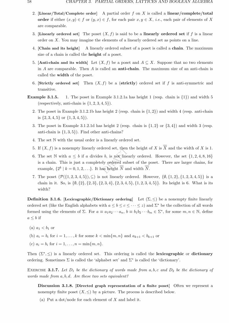
DRAFT

58 CHAPTER 3. PARTIAL ORDERS, LATTICES AND BOOLEAN ALGEBRA

2. [Linear/Total/Complete order] A partial order f on X is called a linear/complete/total

order if either (x, y) ∈ f or (y, x) ∈ f , for each pair x, y ∈ X, i.e., each pair of elements of X

are comparable.

3. [Linearly ordered set] The poset (X, f) is said to be a linearly ordered set if f is a linear

order on X. You may imagine the elements of a linearly ordered set as points on a line.

4. [Chain and its height] A linearly ordered subset of a poset is called a chain. The maximum

size of a chain is called the height of a poset.

5. [Anti-chain and its width] Let (X, f) be a poset and A ⊆ X. Suppose that no two elements

in A are comparable. Then A is called an anti-chain. The maximum size of an anti-chain is

called the width of the poset.

6. [Strictly ordered set] Then (X, f) be a (strictly) ordered set if f is anti-symmetric and

transitive.

Example 3.1.5. 1. The poset in Example 3.1.2.1a has height 1 (resp. chain is 1) and width 5

(respectively, anti-chain is 1, 2, 3, 4, 5).2. The poset in Example 3.1.2.1b has height 2 (resp. chain is 1, 2) and width 4 (resp. anti-chain

is 2, 3, 4, 5 or 1, 3, 4, 5).3. The poset in Example 3.1.2.1d has height 2 (resp. chain is 1, 2 or 3, 4) and width 3 (resp.

anti-chain is 1, 3, 5). Find other anti-chains?

4. The set N with the usual order is a linearly ordered set.

5. If (X, f) is a nonempty linearly ordered set, then the height of X is X and the width of X is 1.

6. The set N with a ≤ b if a divides b, is not linearly ordered. However, the set 1, 2, 4, 8, 16is a chain. This is just a completely ordered subset of the poset. There are larger chains, for

example, 2k | k = 0, 1, 2, . . .. It has height N and width N .

7. The poset (P(1, 2, 3, 4, 5),⊆) is not linearly ordered. However, ∅, 1, 2, 1, 2, 3, 4, 5 is a

chain in it. So, is ∅, 2, 2, 3, 2, 3, 4, 2, 3, 4, 5, 1, 2, 3, 4, 5. Its height is 6. What is its

width?

Definition 3.1.6. [Lexicographic/Dictionary ordering] Let (Σ,≤) be a nonempty finite linearly

ordered set (like the English alphabets with a ≤ b ≤ c ≤ · · · ≤ z) and Σ∗ be the collection of all words

formed using the elements of Σ. For a ≡ a1a2 · · · an, b ≡ b1b2 · · · bm ∈ Σ∗, for some m,n ∈ N, define

a ≤ b if

(a) a1 < b1 or

(b) ai = bi for i = 1, . . . , k for some k < minm,n and ak+1 < bk+1 or

(c) ai = bi for i = 1, . . . , n = minm,n.

Then (Σ∗,≤) is a linearly ordered set. This ordering is called the lexicographic or dictionary

ordering. Sometimes Σ is called the ‘alphabet set’ and Σ∗ is called the ‘dictionary’.

Exercise 3.1.7. Let D1 be the dictionary of words made from a, b, c and D2 be the dictionary of

words made from a, b, d. Are these two sets equivalent?

Discussion 3.1.8. [Directed graph representation of a finite poset] Often we represent a

nonempty finite poset (X,≤) by a picture. The process is described below.

(a) Put a dot/node for each element of X and label it.

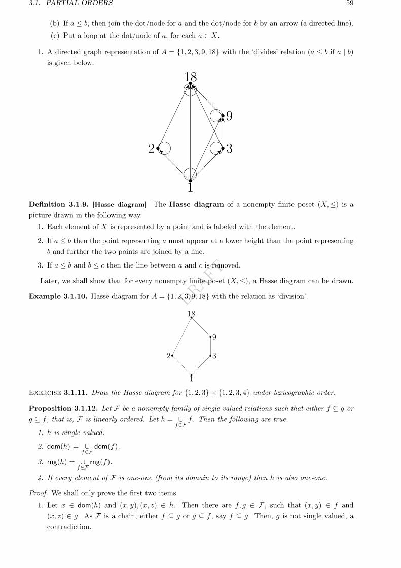
DRAFT

3.1. PARTIAL ORDERS 59

(b) If a ≤ b, then join the dot/node for a and the dot/node for b by an arrow (a directed line).

(c) Put a loop at the dot/node of a, for each a ∈ X.

1. A directed graph representation of A = 1, 2, 3, 9, 18 with the ‘divides’ relation (a ≤ b if a | b)is given below.

1

2 3

9

18

Definition 3.1.9. [Hasse diagram] The Hasse diagram of a nonempty finite poset (X,≤) is a

picture drawn in the following way.

1. Each element of X is represented by a point and is labeled with the element.

2. If a ≤ b then the point representing a must appear at a lower height than the point representing

b and further the two points are joined by a line.

3. If a ≤ b and b ≤ c then the line between a and c is removed.

Later, we shall show that for every nonempty finite poset (X,≤), a Hasse diagram can be drawn.

Example 3.1.10. Hasse diagram for A = 1, 2, 3, 9, 18 with the relation as ‘division’.

1

2 3

9

18

Exercise 3.1.11. Draw the Hasse diagram for 1, 2, 3 × 1, 2, 3, 4 under lexicographic order.

Proposition 3.1.12. Let F be a nonempty family of single valued relations such that either f ⊆ g or

g ⊆ f , that is, F is linearly ordered. Let h = ∪f∈F

f . Then the following are true.

1. h is single valued.

2. dom(h) = ∪f∈F

dom(f).

3. rng(h) = ∪f∈F

rng(f).

4. If every element of F is one-one (from its domain to its range) then h is also one-one.

Proof. We shall only prove the first two items.

1. Let x ∈ dom(h) and (x, y), (x, z) ∈ h. Then there are f, g ∈ F , such that (x, y) ∈ f and

(x, z) ∈ g. As F is a chain, either f ⊆ g or g ⊆ f , say f ⊆ g. Then, g is not single valued, a

contradiction.

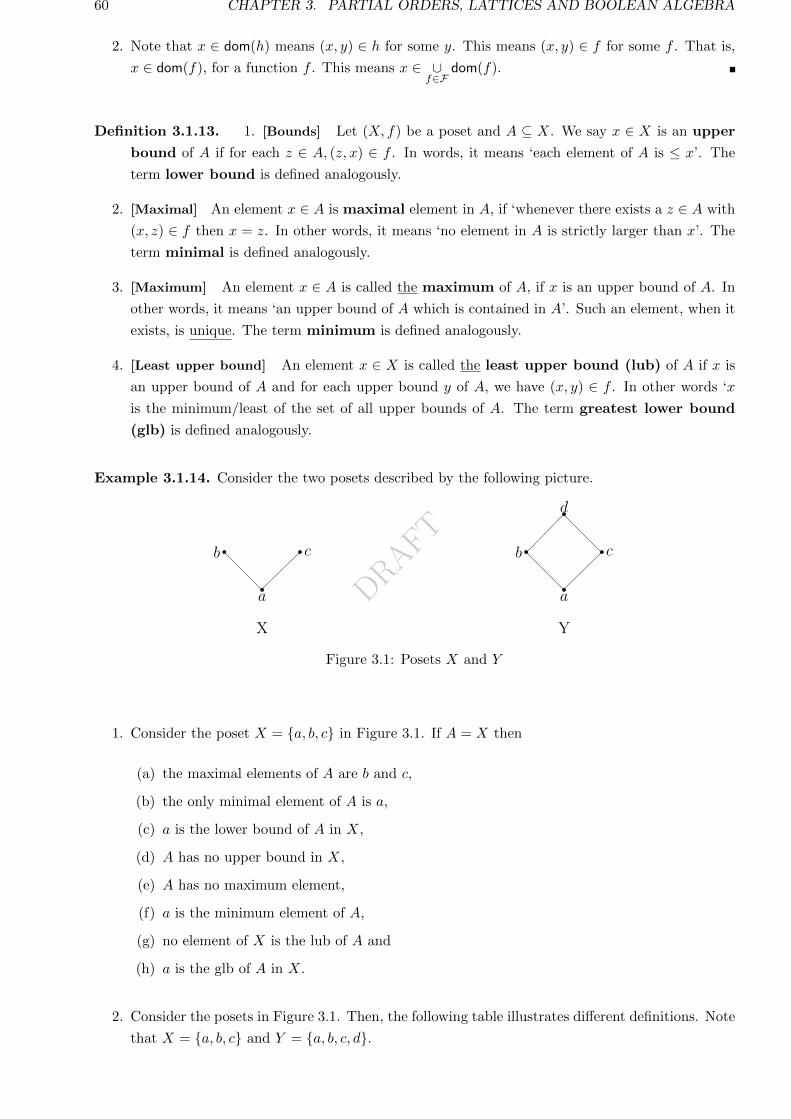
DRAFT


2. Note that x ∈ dom(h) means (x, y) ∈ h for some y. This means (x, y) ∈ f for some f . That is,

x ∈ dom(f), for a function f . This means x ∈ ∪f∈F

dom(f).

Definition 3.1.13. 1. [Bounds] Let (X, f) be a poset and A ⊆ X. We say x ∈ X is an upper

bound of A if for each z ∈ A, (z, x) ∈ f . In words, it means ‘each element of A is ≤ x’. The

term lower bound is defined analogously.

2. [Maximal] An element x ∈ A is maximal element in A, if ‘whenever there exists a z ∈ A with

(x, z) ∈ f then x = z. In other words, it means ‘no element in A is strictly larger than x’. The

term minimal is defined analogously.

3. [Maximum] An element x ∈ A is called the maximum of A, if x is an upper bound of A. In

other words, it means ‘an upper bound of A which is contained in A’. Such an element, when it

exists, is unique. The term minimum is defined analogously.

4. [Least upper bound] An element x ∈ X is called the least upper bound (lub) of A if x is

an upper bound of A and for each upper bound y of A, we have (x, y) ∈ f . In other words ‘x

is the minimum/least of the set of all upper bounds of A. The term greatest lower bound

(glb) is defined analogously.

Example 3.1.14. Consider the two posets described by the following picture.

a

b c

X

a

b c

d

Y

1

Figure 3.1: Posets X and Y

1. Consider the poset X = a, b, c in Figure 3.1. If A = X then

(a) the maximal elements of A are b and c,

(b) the only minimal element of A is a,

(c) a is the lower bound of A in X,

(d) A has no upper bound in X,

(e) A has no maximum element,

(f) a is the minimum element of A,

(g) no element of X is the lub of A and

(h) a is the glb of A in X.

2. Consider the posets in Figure 3.1. Then, the following table illustrates different definitions. Note

that X = a, b, c and Y = a, b, c, d.

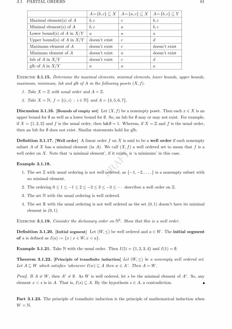
DRAFT


A=b, c ⊆ X A=a, c ⊆ X A=b, c ⊆ YMaximal element(s) of A b, c c b, c

Minimal element(s) of A b, c a b, c

Lower bound(s) of A in X/Y a a a

Upper bound(s) of A in X/Y doesn’t exist c d

Maximum element of A doesn’t exist c doesn’t exist

Minimum element of A doesn’t exist a doesn’t exist

lub of A in X/Y doesn’t exist c d

glb of A in X/Y a a a

Exercise 3.1.15. Determine the maximal elements, minimal elements, lower bounds, upper bounds,

maximum, minimum, lub and glb of A in the following posets (X, f).

1. Take X = Z with usual order and A = Z.

2. Take X = N, f = (i, i) : i ∈ N and A = 4, 5, 6, 7.

Discussion 3.1.16. [Bounds of empty set] Let (X, f) be a nonempty poset. Then each x ∈ X is an

upper bound for ∅ as well as a lower bound for ∅. So, an lub for ∅ may or may not exist. For example,

if X = 1, 2, 3 and f is the usual order, then lub ∅ = 1. Whereas, if X = Z and f is the usual order,

then an lub for ∅ does not exist. Similar statements hold for glb.

Definition 3.1.17. [Well order] A linear order f on X is said to be a well order if each nonempty

subset A of X has a minimal element (in A). We call (X, f) a well ordered set to mean that f is a

well order on X. Note that ‘a minimal element’, if it exists, is ‘a minimum’ in this case.

Example 3.1.18.

1. The set Z with usual ordering is not well ordered, as −1,−2, . . . , is a nonempty subset with

no minimal element.

2. The ordering 0 ≤ 1 ≤ −1 ≤ 2 ≤ −2 ≤ 3 ≤ −3 ≤ · · · describes a well order on Z.

3. The set N with the usual ordering is well ordered.

4. The set R with the usual ordering is not well ordered as the set (0, 1) doesn’t have its minimal

element in (0, 1).

Exercise 3.1.19. Consider the dictionary order on N2. Show that this is a well order.

Definition 3.1.20. [Initial segment] Let (W,≤) be well ordered and a ∈W . The initial segment

of a is defined as I(a) := x | x ∈W,x < a.

Example 3.1.21. Take N with the usual order. Then I(5) = 1, 2, 3, 4 and I(1) = ∅.

Theorem 3.1.22. [Principle of transfinite induction] Let (W,≤) be a nonempty well ordered set.

Let A ⊆W which satisfies ‘whenever I(w) ⊆ A then w ∈ A’. Then A = W .

Proof. If A 6= W , then Ac 6= ∅. As W is well ordered, let s be the minimal element of Ac. So, any

element x < s is in A. That is, I(s) ⊆ A. By the hypothesis s ∈ A, a contradiction.

Fact 3.1.23. The principle of transfinite induction is the principle of mathematical induction when

W = N.

DRAFT


Proof. To see this, let p(n) be a statement which needs to be proved by mathematical induction. Put

A = n ∈ N | p(n) is true. Assume that we have been able to show that ‘I(n) ⊆ A ⇒ n ∈ A’.

It means, we have shown that 1 ∈ A, as ∅ = I(1) ⊆ A. Also we have shown that for n ≥ 2, if

p(1), . . . , p(n− 1) are true then p(n) is true as well, as I(n) = 1, 2, . . . , n− 1.

Definition 3.1.24. [Product of sets] Recall that the product A1 × A2 = (x1, x2) | xi ∈ Ai may

be written as(f(1), f(2)

)∣∣f : 1, 2 → A1 ∪A2 is a function with f(1) ∈ A1, f(2) ∈ A2

.

Moreover, if A1 and A2 are finite sets then |A1 ×A2| = |A1| · |A2|. In general, we define the product

of the sets in Aαα∈L, L 6= ∅, as∏α∈L

Aα =f | f : L→ ∪

α∈LAα is a function with f(α) ∈ Aα, for each α ∈ L

.

Example 3.1.25. 1. Take L = N and An = 0, 1. Then∏α∈L

Aα is the class of functions f : L→0, 1. That is, it is the class of all 0-1-sequences.

2. By definition, product of a class of sets among which one of them is ∅ is empty.

What about product of a class of sets in which no set is empty? Is it nonempty? This could not be

proved using the standard set theory. In fact, it is now proved that this question cannot be answered

using the standard set theory. So, a new axiom, called the axiom of choice, was introduced.

Axiom 3.1.26. [Axiom of Choice] The product of a nonempty class of nonempty sets is nonempty.

Proposition 3.1.27. [Injection-Surjection] Let A and B be nonempty sets. Then, there is a surjec-

tion g : A→ B if and only if there is an injection f : B → A.

Proof. Let g : A→ B be onto. We shall find an injection from B to A. To start with, notice that for

each b ∈ B, the set g−1(b) 6= ∅. Then, by axiom of choice∏b∈B

g−1(b) 6= ∅. Let f ∈ ∏b∈B

g−1(b). Then,

by Definition 3.1.24, f : B → A is a function. As g is a function, g−1(b)’s are disjoint and hence f is

one-one.

Conversely, let f : B → A be one-one. Fix an element b ∈ B. Define g : A→ B as

g(x) =

f−1(x), if x ∈ f(B),

b, if x ∈ A \ f(B).

Observe that g is onto.

Definition 3.1.28. [Family of finite character] A class F of sets is called a family of finite

character if it satisfies: ‘A ∈ F if and only if each finite subset of A is also in F ’.

Example 3.1.29. 1. is a family of finite character.

2. Power sets are families of finite character.

3. ∅, 1, 2 is a family of finite character.

4. If A ∩B = ∅, then P(A) ∪ P(B) is a family of finite character.

5. The set ∅ ∪ a | a 6= 0, a ∈ R is a family of finite character. This is the class of linearly

independent sets in R.

DRAFT


6. Let V be a non trivial vector space and F be the class of linearly independent subsets of V.

Then F is a family of finite character.

Exercise 3.1.30. 1. Let L = A1 = A2 = A3 = 1, 2, 3. Is the set∏α∈L

Aα equal to the class of

functions f : 1, 2, 3 → 1, 2, 3? Give reasons for your answer.

2. Give sets An, n ∈ N such that∏n∈N

An has 6 elements. Give another.1

Some equivalent axioms of axiom of choice

[Axiom of choice] Cartesian product of a nonempty collection of nonempty sets is nonempty.

[Zorn’s lemma] A partially ordered set in which every chain has an upper bound, has a

maximal element.

[Zermelo’s well ordering principle] Every set can be well ordered.

[Hausdorff’s maximality principle] Every nonempty partially ordered set contains a max-

imal chain.

[Tukey’s lemma] Every nonempty family of finite character has a maximal element.

Exercise 3.1.31. 1. Does there exist a poset with exactly 5 maximal chains of size (number of

elements in it) 2, 3, 4, 5, 6, respectively and 2 maximal elements? If yes, draw the Hasse diagram.

If no, argue it.

2. Let (X, f) be a nonempty poset and ∅ 6= Y ⊆ X. Define fY = (a, b) ∈ f | a, b ∈ Y . Show

that fY is a partial order on Y . This is the induced partial order on Y .

3. Apply induction to show that a nonempty finite poset has a maximal element and a minimal

element.

Discussion 3.1.32. [Drawing the Hasse diagram of a finite poset (X, f)] Let x1, . . . , xk be the

minimal elements of X. Draw k points on the same horizontal line and label them x1, . . . , xk. Now

consider Y = X \x1, . . . , xk and fY . By induction, the picture of (Y, fY ) can be drawn. Put it above

those k dots. Let y1, . . . , ym be the minimal elements of Y . Now, draw the lines (xi, yj) if (xi, yj) ∈ f .

This is the Hasse diagram of (X, f).

Discussion 3.1.33. [Existence of Hamel basis] Let V be a vector space with at least two elements.

Recall that the collection F of linearly independent subsets of V is a family of finite character. Recall

that a basis or a Hamel basis is a maximal linearly independent subset of V. As V has at least 2

elements, it has a nonzero element, say a. Then a ∈ F . Hence, F 6= ∅. Thus, by Tukey’s lemma,

the set F has a maximal element. This maximal set is the required basis. Hence, we have proved that

every vector space with at least 2 elements has a Hamel basis.

Exercise 3.1.34. 1. Let n ∈ N. Define Pn = k ∈ N | k divides n. Define a relation ≤n on Pn

as ≤n= (a, b) | a divides b. Show that (Pn,≤n) is a poset, for each n ∈ N. Give a necessary

and sufficient condition on n so that (Pn,≤n) is a completely ordered set.

2. Take X =

(1, 1), (1, 2), (1, 3), . . .∪

(2, 1)(3, 1), (4, 1), . . .

. The ordering defined is

f = ∪m,n ∈ Nm ≤ n

((1,m), (1, n)

)⋃∪

m,n ∈ Nm ≤ n

((m, 1), (n, 1)

).

Does X have any maximal or minimal elements? Is X linearly ordered? Is it true that every

nonempty set has a minimal element? Is it true that every nonempty set has a minimum? What

type of nonempty sets always have a minimum?

1When we ask for more than one example, we encourage the reader to get examples of different types, if possible.

DRAFT


3. Prove or disprove:

(a) There are at least 5 functions f : R→ R which are partial orders.

(b) Let S be the set of sequences (xn), with xn ∈ 0, 1, . . . , 9, for each n ∈ N, such that ‘if

xk < xk+1, then xk+1 = xk+2 = · · · ‘. Then S is countable.

(c) Take N with usual order. Then the dictionary order on N2 is a well order.

(d) Let S be the set of all non-increasing sequences made with natural numbers. Then S is

countable.

(e) Let S be the set of all non-decreasing sequences made with natural numbers. Then S is

countable.

(f) Take N with usual order and N2 with the dictionary order. Then any nonempty subset of

N2 which is bounded above has a lub.

(g) Every nonempty countable linearly ordered set is well ordered with respect to the same

ordering.

(h) Every nonempty countable chain which is bounded below, in a partially ordered set, is well

ordered with respect to the same ordering.

(i) The set Q can be well ordered.

(j) For a fixed n ∈ N, let An and Bn be non-empty sets and let Rn be a one-one relation from

An to Bn. Then, ∩nRn is a one-one relation.

(k) Let S be the set of words with length at most 8 using letters from 3, A, a, b, C, c. We want

to define a lexicographic order on S to make it a dictionary. There are more than 500 ways

to do that.

(l) An infinite poset in which each nonempty finite set has a minimum, must be linearly ordered.

(m) A nonempty finite poset in which each nonempty finite set has a minimum, must be well

ordered.

(n) An infinite poset in which each nonempty finite set has a minimum, must be well ordered.

4. Let S = (x, y) : x2 + y2 = 1, x ≥ 0. It is a relation from R to R. Draw a picture of the inverse

of this relation.

5. Construct the Hasse diagram for the ⊆ relation on P(a, b, c).6. Draw the Hasse diagram for the partial order describing the ‘divides’ relations on the set 2, 3, 4, 5, 6, 7, 8.7. Draw the Hasse diagram of 1, 2, 3, 6, 9, 18 with ‘divides’ relation.

(a) What is its height? What is its width.

(b) Let A = 2, 3, 6. What are the maximal elements, minimal elements, maximum, minimum,

lower bounds, upper bounds, glb and lub of A.

Exercise 3.1.35. ∗

1. Show that the following three definitions are equivalent.

(a) A set X is finite if either X = ∅ or X = 1, 2, . . . , n, for some n ∈ N.

(b) [Tarski] A set X is finite if and only if every nonempty family of subsets of X has a

minimal element.

(c) [Dedekind] A set is infinite if it is equivalent to a proper subset of itself. A set is finite if

it is not infinite.

2. Let (X, f) be a nonempty poset. Show that there exists a linear order g on X such that f ⊆ g.

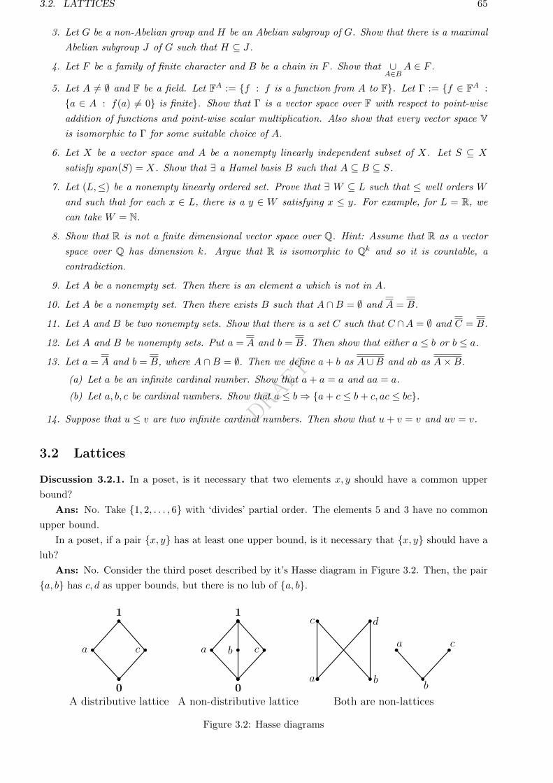
DRAFT

3.2. LATTICES 65

3. Let G be a non-Abelian group and H be an Abelian subgroup of G. Show that there is a maximal

Abelian subgroup J of G such that H ⊆ J .

4. Let F be a family of finite character and B be a chain in F . Show that ∪A∈B

A ∈ F .

5. Let A 6= ∅ and F be a field. Let FA := f : f is a function from A to F. Let Γ := f ∈ FA :

a ∈ A : f(a) 6= 0 is finite. Show that Γ is a vector space over F with respect to point-wise

addition of functions and point-wise scalar multiplication. Also show that every vector space Vis isomorphic to Γ for some suitable choice of A.

6. Let X be a vector space and A be a nonempty linearly independent subset of X. Let S ⊆ X

satisfy span(S) = X. Show that ∃ a Hamel basis B such that A ⊆ B ⊆ S.

7. Let (L,≤) be a nonempty linearly ordered set. Prove that ∃ W ⊆ L such that ≤ well orders W

and such that for each x ∈ L, there is a y ∈ W satisfying x ≤ y. For example, for L = R, we

can take W = N.

8. Show that R is not a finite dimensional vector space over Q. Hint: Assume that R as a vector

space over Q has dimension k. Argue that R is isomorphic to Qk and so it is countable, a

contradiction.

9. Let A be a nonempty set. Then there is an element a which is not in A.

10. Let A be a nonempty set. Then there exists B such that A ∩B = ∅ and A = B.

11. Let A and B be two nonempty sets. Show that there is a set C such that C ∩A = ∅ and C = B.

12. Let A and B be nonempty sets. Put a = A and b = B. Then show that either a ≤ b or b ≤ a.

13. Let a = A and b = B, where A ∩B = ∅. Then we define a+ b as A ∪B and ab as A×B.

(a) Let a be an infinite cardinal number. Show that a+ a = a and aa = a.

(b) Let a, b, c be cardinal numbers. Show that a ≤ b⇒ a+ c ≤ b+ c, ac ≤ bc.

14. Suppose that u ≤ v are two infinite cardinal numbers. Then show that u+ v = v and uv = v.

3.2 Lattices

Discussion 3.2.1. In a poset, is it necessary that two elements x, y should have a common upper

bound?

Ans: No. Take 1, 2, . . . , 6 with ‘divides’ partial order. The elements 5 and 3 have no common

upper bound.

In a poset, if a pair x, y has at least one upper bound, is it necessary that x, y should have a

lub?

Ans: No. Consider the third poset described by it’s Hasse diagram in Figure 3.2. Then, the pair

a, b has c, d as upper bounds, but there is no lub of a, b.

a

0

c

1

A distributive lattice

a

0

b c

1

A non-distributive lattice

a

c

b

d

a c

b

Both are non-lattices

1

Figure 3.2: Hasse diagrams

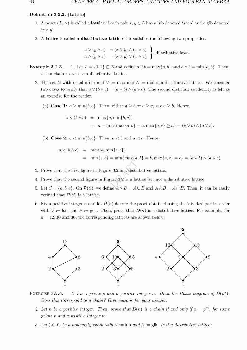
DRAFT


Definition 3.2.2. [Lattice]

1. A poset (L,≤) is called a lattice if each pair x, y ∈ L has a lub denoted ‘x∨y’ and a glb denoted

‘x ∧ y’.

2. A lattice is called a distributive lattice if it satisfies the following two properties.

x ∨ (y ∧ z) = (x ∨ y) ∧ (x ∨ z).x ∧ (y ∨ z) = (x ∧ y) ∨ (x ∧ z).

distributive laws

Example 3.2.3. 1. Let L = 0, 1 ⊆ Z and define a∨ b = maxa, b and a∧ b = mina, b. Then,

L is a chain as well as a distributive lattice.

2. The set N with usual order and ∨ := max and ∧ := min is a distributive lattice. We consider

two cases to verify that a ∨ (b ∧ c) = (a ∨ b) ∧ (a ∨ c). The second distributive identity is left as

an exercise for the reader.

(a) Case 1: a ≥ minb, c. Then, either a ≥ b or a ≥ c, say a ≥ b. Hence,

a ∨ (b ∧ c) = maxa,minb, c= a = minmaxa, b = a,maxa, c ≥ a = (a ∨ b) ∧ (a ∨ c).

(b) Case 2: a < minb, c. Then, a < b and a < c. Hence,

a ∨ (b ∧ c) = maxa,minb, c= minb, c = minmaxa, b = b,maxa, c = c = (a ∨ b) ∧ (a ∨ c).

3. Prove that the first figure in Figure 3.2 is a distributive lattice.

4. Prove that the second figure in Figure 3.2 is a lattice but not a distributive lattice.

5. Let S = a, b, c. On P(S), we define A∨B = A∪B and A∧B = A∩B. Then, it can be easily

verified that P(S) is a lattice.

6. Fix a positive integer n and let D(n) denote the poset obtained using the ‘divides’ partial order

with ∨ := lcm and ∧ := gcd. Then, prove that D(n) is a distributive lattice. For example, for

n = 12, 30 and 36, the corresponding lattices are shown below.

2

1

3

12

4 6

2

1

5

30

6 10

3

15

2

1

3

36

4 6 9

1812

1

Exercise 3.2.4. 1. Fix a prime p and a positive integer n. Draw the Hasse diagram of D(pn).

Does this correspond to a chain? Give reasons for your answer.

2. Let n be a positive integer. Then, prove that D(n) is a chain if and only if n = pm, for some

prime p and a positive integer m.

3. Let (X, f) be a nonempty chain with ∨ := lub and ∧ := glb. Is it a distributive lattice?

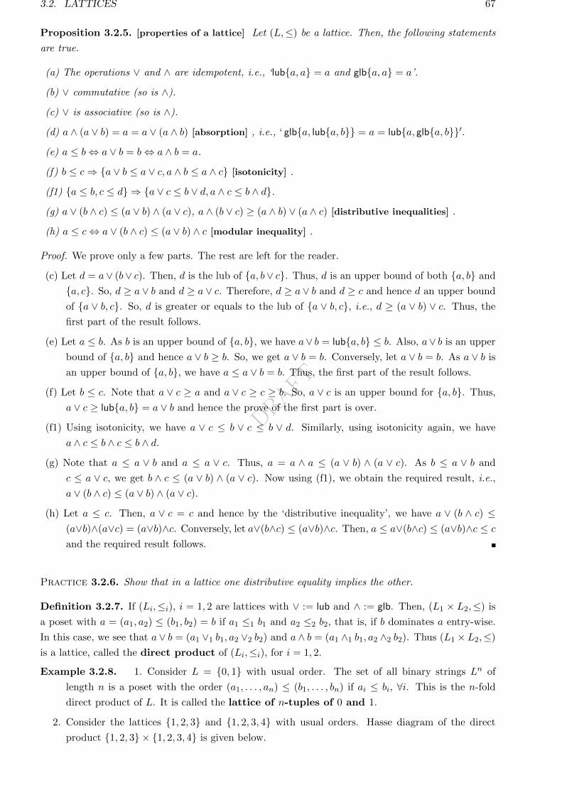
DRAFT

3.2. LATTICES 67

Proposition 3.2.5. [properties of a lattice] Let (L,≤) be a lattice. Then, the following statements

are true.

(a) The operations ∨ and ∧ are idempotent, i.e., ‘luba, a = a and glba, a = a’.

(b) ∨ commutative (so is ∧).

(c) ∨ is associative (so is ∧).

(d) a ∧ (a ∨ b) = a = a ∨ (a ∧ b) [absorption] , i.e., ‘ glba, luba, b = a = luba, glba, b′.(e) a ≤ b⇔ a ∨ b = b⇔ a ∧ b = a.

(f) b ≤ c⇒ a ∨ b ≤ a ∨ c, a ∧ b ≤ a ∧ c [isotonicity] .

(f1) a ≤ b, c ≤ d ⇒ a ∨ c ≤ b ∨ d, a ∧ c ≤ b ∧ d.(g) a ∨ (b ∧ c) ≤ (a ∨ b) ∧ (a ∨ c), a ∧ (b ∨ c) ≥ (a ∧ b) ∨ (a ∧ c) [distributive inequalities] .

(h) a ≤ c⇔ a ∨ (b ∧ c) ≤ (a ∨ b) ∧ c [modular inequality] .

Proof. We prove only a few parts. The rest are left for the reader.

(c) Let d = a∨ (b∨ c). Then, d is the lub of a, b∨ c. Thus, d is an upper bound of both a, b and

a, c. So, d ≥ a ∨ b and d ≥ a ∨ c. Therefore, d ≥ a ∨ b and d ≥ c and hence d an upper bound

of a ∨ b, c. So, d is greater or equals to the lub of a ∨ b, c, i.e., d ≥ (a ∨ b) ∨ c. Thus, the

first part of the result follows.

(e) Let a ≤ b. As b is an upper bound of a, b, we have a∨ b = luba, b ≤ b. Also, a∨ b is an upper

bound of a, b and hence a ∨ b ≥ b. So, we get a ∨ b = b. Conversely, let a ∨ b = b. As a ∨ b is

an upper bound of a, b, we have a ≤ a ∨ b = b. Thus, the first part of the result follows.

(f) Let b ≤ c. Note that a ∨ c ≥ a and a ∨ c ≥ c ≥ b. So, a ∨ c is an upper bound for a, b. Thus,

a ∨ c ≥ luba, b = a ∨ b and hence the prove of the first part is over.

(f1) Using isotonicity, we have a ∨ c ≤ b ∨ c ≤ b ∨ d. Similarly, using isotonicity again, we have

a ∧ c ≤ b ∧ c ≤ b ∧ d.

(g) Note that a ≤ a ∨ b and a ≤ a ∨ c. Thus, a = a ∧ a ≤ (a ∨ b) ∧ (a ∨ c). As b ≤ a ∨ b and

c ≤ a ∨ c, we get b ∧ c ≤ (a ∨ b) ∧ (a ∨ c). Now using (f1), we obtain the required result, i.e.,

a ∨ (b ∧ c) ≤ (a ∨ b) ∧ (a ∨ c).(h) Let a ≤ c. Then, a ∨ c = c and hence by the ‘distributive inequality’, we have a ∨ (b ∧ c) ≤

(a∨b)∧(a∨c) = (a∨b)∧c. Conversely, let a∨(b∧c) ≤ (a∨b)∧c. Then, a ≤ a∨(b∧c) ≤ (a∨b)∧c ≤ cand the required result follows.

Practice 3.2.6. Show that in a lattice one distributive equality implies the other.

Definition 3.2.7. If (Li,≤i), i = 1, 2 are lattices with ∨ := lub and ∧ := glb. Then, (L1 × L2,≤) is

a poset with a = (a1, a2) ≤ (b1, b2) = b if a1 ≤1 b1 and a2 ≤2 b2, that is, if b dominates a entry-wise.

In this case, we see that a ∨ b = (a1 ∨1 b1, a2 ∨2 b2) and a ∧ b = (a1 ∧1 b1, a2 ∧2 b2). Thus (L1 ×L2,≤)

is a lattice, called the direct product of (Li,≤i), for i = 1, 2.

Example 3.2.8. 1. Consider L = 0, 1 with usual order. The set of all binary strings Ln of

length n is a poset with the order (a1, . . . , an) ≤ (b1, . . . , bn) if ai ≤ bi, ∀i. This is the n-fold

direct product of L. It is called the lattice of n-tuples of 0 and 1.

2. Consider the lattices 1, 2, 3 and 1, 2, 3, 4 with usual orders. Hasse diagram of the direct

product 1, 2, 3 × 1, 2, 3, 4 is given below.

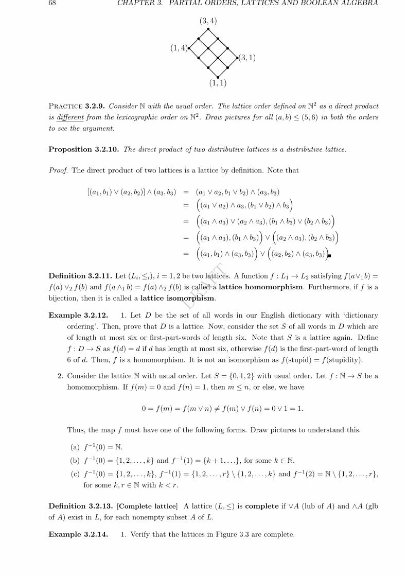
DRAFT


(1, 1)

(3, 1)

(3, 4)

(1, 4)

Practice 3.2.9. Consider N with the usual order. The lattice order defined on N2 as a direct product

is different from the lexicographic order on N2. Draw pictures for all (a, b) ≤ (5, 6) in both the orders

to see the argument.

Proposition 3.2.10. The direct product of two distributive lattices is a distributive lattice.

Proof. The direct product of two lattices is a lattice by definition. Note that

[(a1, b1) ∨ (a2, b2)] ∧ (a3, b3) = (a1 ∨ a2, b1 ∨ b2) ∧ (a3, b3)

=(

(a1 ∨ a2) ∧ a3, (b1 ∨ b2) ∧ b3)

=(

(a1 ∧ a3) ∨ (a2 ∧ a3), (b1 ∧ b3) ∨ (b2 ∧ b3))

=(

(a1 ∧ a3), (b1 ∧ b3))∨(

(a2 ∧ a3), (b2 ∧ b3))

=(

(a1, b1) ∧ (a3, b3))∨(

(a2, b2) ∧ (a3, b3))

Definition 3.2.11. Let (Li,≤i), i = 1, 2 be two lattices. A function f : L1 → L2 satisfying f(a∨1b) =

f(a) ∨2 f(b) and f(a ∧1 b) = f(a) ∧2 f(b) is called a lattice homomorphism. Furthermore, if f is a

bijection, then it is called a lattice isomorphism.

Example 3.2.12. 1. Let D be the set of all words in our English dictionary with ‘dictionary

ordering’. Then, prove that D is a lattice. Now, consider the set S of all words in D which are

of length at most six or first-part-words of length six. Note that S is a lattice again. Define

f : D → S as f(d) = d if d has length at most six, otherwise f(d) is the first-part-word of length

6 of d. Then, f is a homomorphism. It is not an isomorphism as f(stupid) = f(stupidity).

2. Consider the lattice N with usual order. Let S = 0, 1, 2 with usual order. Let f : N→ S be a

homomorphism. If f(m) = 0 and f(n) = 1, then m ≤ n, or else, we have

0 = f(m) = f(m ∨ n) 6= f(m) ∨ f(n) = 0 ∨ 1 = 1.

Thus, the map f must have one of the following forms. Draw pictures to understand this.

(a) f−1(0) = N.

(b) f−1(0) = 1, 2, . . . , k and f−1(1) = k + 1, . . ., for some k ∈ N.

(c) f−1(0) = 1, 2, . . . , k, f−1(1) = 1, 2, . . . , r \ 1, 2, . . . , k and f−1(2) = N \ 1, 2, . . . , r,for some k, r ∈ N with k < r.

Definition 3.2.13. [Complete lattice] A lattice (L,≤) is complete if ∨A (lub of A) and ∧A (glb

of A) exist in L, for each nonempty subset A of L.

Example 3.2.14. 1. Verify that the lattices in Figure 3.3 are complete.

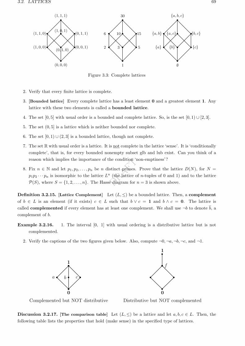
DRAFT

3.2. LATTICES 69

(1, 0, 0)

(0, 0, 0)

(0, 0, 1)

(1, 1, 1)

(1, 1, 0)(1, 0, 1)

(0, 1, 0)

(0, 1, 1)

2

1

5

30

6 10

3

15

a

∅

c

a, b, c

a, b a, c

b

b, c

1

Figure 3.3: Complete lattices

2. Verify that every finite lattice is complete.

3. [Bounded lattice] Every complete lattice has a least element 0 and a greatest element 1. Any

lattice with these two elements is called a bounded lattice.

4. The set [0, 5] with usual order is a bounded and complete lattice. So, is the set [0, 1) ∪ [2, 3].

5. The set (0, 5] is a lattice which is neither bounded nor complete.

6. The set [0, 1) ∪ (2, 3] is a bounded lattice, though not complete.

7. The set R with usual order is a lattice. It is not complete in the lattice ‘sense’. It is ‘conditionally

complete’, that is, for every bounded nonempty subset glb and lub exist. Can you think of a

reason which implies the importance of the condition ‘non-emptiness’?

8. Fix n ∈ N and let p1, p2, . . . , pn be n distinct primes. Prove that the lattice D(N), for N =

p1p2 · · · pn is isomorphic to the lattice Ln (the lattice of n-tuples of 0 and 1) and to the lattice

P(S), where S = 1, 2, . . . , n. The Hasse diagram for n = 3 is shown above.

Definition 3.2.15. [Lattice Complement] Let (L,≤) be a bounded lattice. Then, a complement

of b ∈ L is an element (if it exists) c ∈ L such that b ∨ c = 1 and b ∧ c = 0. The lattice is

called complemented if every element has at least one complement. We shall use ¬b to denote b, a

complement of b.

Example 3.2.16. 1. The interval [0, 1] with usual ordering is a distributive lattice but is not

complemented.

2. Verify the captions of the two figures given below. Also, compute ¬0,¬a,¬b,¬c, and ¬1.

a

0

b c

1

Complemented but NOT distributive

0

1

f

Distributive but NOT complemented

1

Discussion 3.2.17. [The comparison table] Let (L,≤) be a lattice and let a, b, c ∈ L. Then, the

following table lists the properties that hold (make sense) in the specified type of lattices.

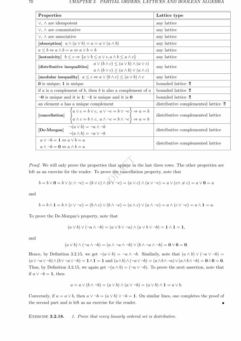
DRAFT


Properties Lattice type

∨, ∧ are idempotent any lattice

∨, ∧ are commutative any lattice

∨, ∧ are associative any lattice

[absorption] a ∧ (a ∨ b) = a = a ∨ (a ∧ b) any lattice

a ≤ b⇔ a ∧ b = a⇔ a ∨ b = b any lattice

[isotonicity] b ≤ c⇒ a ∨ b ≤ a ∨ c, a ∧ b ≤ a ∧ c any lattice

[distributive inequalities]a ∨ (b ∧ c) ≤ (a ∨ b) ∧ (a ∨ c)a ∧ (b ∨ c) ≥ (a ∧ b) ∨ (a ∧ c)

any lattice

[modular inequality] a ≤ c⇔ a ∨ (b ∧ c) ≤ (a ∨ b) ∧ c any lattice

0 is unique; 1 is unique bounded lattice !!

if a is a complement of b, then b is also a complement of a bounded lattice !!

¬0 is unique and it is 1; ¬1 is unique and it is 0 bounded lattice !!

an element a has a unique complement distributive complemented lattice !!

[cancellation]

a ∨ c = b ∨ c, a ∨ ¬c = b ∨ ¬c

⇒ a = b

a ∧ c = b ∧ c, a ∧ ¬c = b ∧ ¬c⇒ a = b

distributive complemented lattice

[De-Morgan]¬(a ∨ b) = ¬a ∧ ¬b¬(a ∧ b) = ¬a ∨ ¬b

distributive complemented lattice

a ∨ ¬b = 1⇔ a ∨ b = a

a ∧ ¬b = 0⇔ a ∧ b = adistributive complemented lattice

Proof. We will only prove the properties that appear in the last three rows. The other properties are

left as an exercise for the reader. To prove the cancellation property, note that

b = b ∨ 0 = b ∨ (c ∧ ¬c) = (b ∨ c) ∧ (b ∨ ¬c) = (a ∨ c) ∧ (a ∨ ¬c) = a ∨ (c∧ 6= c) = a ∨ 0 = a

and

b = b ∧ 1 = b ∧ (c ∨ ¬c) = (b ∧ c) ∨ (b ∧ ¬c) = (a ∧ c) ∨ (a ∧ ¬c) = a ∧ (c ∨ ¬c) = a ∧ 1 = a.

To prove the De-Morgan’s property, note that

(a ∨ b) ∨ (¬a ∧ ¬b) = (a ∨ b ∨ ¬a) ∧ (a ∨ b ∨ ¬b) = 1 ∧ 1 = 1,

and

(a ∨ b) ∧ (¬a ∧ ¬b) = (a ∧ ¬a ∧ ¬b) ∨ (b ∧ ¬a ∧ ¬b) = 0 ∨ 0 = 0.

Hence, by Definition 3.2.15, we get ¬(a ∨ b) = ¬a ∧ ¬b. Similarly, note that (a ∧ b) ∨ (¬a ∨ ¬b) =

(a∨¬a∨¬b)∧ (b∨¬a∨¬b) = 1∧1 = 1 and (a∧ b)∧ (¬a∨¬b) = (a∧ b∧¬a)∨ (a∧ b∧¬b) = 0∧0 = 0.

Thus, by Definition 3.2.15, we again get ¬(a ∧ b) = (¬a ∨ ¬b). To prove the next assertion, note that

if a ∨ ¬b = 1, then

a = a ∨ (b ∧ ¬b) = (a ∨ b) ∧ (a ∨ ¬b) = (a ∨ b) ∧ 1 = a ∨ b.

Conversely, if a = a ∨ b, then a ∨ ¬b = (a ∨ b) ∨ ¬b = 1. On similar lines, one completes the proof of

the second part and is left as an exercise for the reader.

Exercise 3.2.18. 1. Prove that every linearly ordered set is distributive.

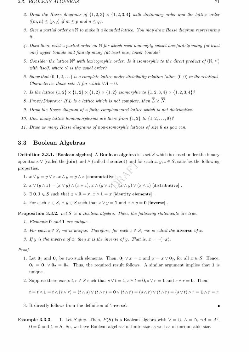
DRAFT

3.3. BOOLEAN ALGEBRAS 71

2. Draw the Hasse diagrams of 1, 2, 3 × 1, 2, 3, 4 with dictionary order and the lattice order

((m,n) ≤ (p, q) if m ≤ p and n ≤ q).

3. Give a partial order on N to make it a bounded lattice. You may draw Hasse diagram representing

it.

4. Does there exist a partial order on N for which each nonempty subset has finitely many (at least

one) upper bounds and finitely many (at least one) lower bounds?

5. Consider the lattice N2 with lexicographic order. Is it isomorphic to the direct product of (N,≤)

with itself, where ≤ is the usual order?

6. Show that 0, 1, 2, . . . is a complete lattice under divisibility relation (allow (0, 0) in the relation).

Characterize those sets A for which ∨A = 0.

7. Is the lattice 1, 2 × 1, 2 × 1, 2 × 1, 2 isomorphic to 1, 2, 3, 4 × 1, 2, 3, 4?8. Prove/Disprove: If L is a lattice which is not complete, then L ≥ N .

9. Draw the Hasse diagram of a finite complemented lattice which is not distributive.

10. How many lattice homomorphisms are there from 1, 2 to 1, 2, . . . , 9?11. Draw as many Hasse diagrams of non-isomorphic lattices of size 6 as you can.

3.3 Boolean Algebras

Definition 3.3.1. [Boolean algebra] A Boolean algebra is a set S which is closed under the binary

operations ∨ (called the join) and ∧ (called the meet) and for each x, y, z ∈ S, satisfies the following

properties.

1. x ∨ y = y ∨ x, x ∧ y = y ∧ x [commutative] .

2. x ∨ (y ∧ z) = (x ∨ y) ∧ (x ∨ z), x ∧ (y ∨ z) = (x ∧ y) ∨ (x ∧ z) [distributive] .

3. ∃ 0,1 ∈ S such that x ∨ 0 = x, x ∧ 1 = x [identity elements] .

4. For each x ∈ S, ∃ y ∈ S such that x ∨ y = 1 and x ∧ y = 0 [inverse] .

Proposition 3.3.2. Let S be a Boolean algebra. Then, the following statements are true.

1. Elements 0 and 1 are unique.

2. For each s ∈ S, ¬s is unique. Therefore, for each x ∈ S, ¬x is called the inverse of x.

3. If y is the inverse of x, then x is the inverse of y. That is, x = ¬(¬x).

Proof.

1. Let 01 and 02 be two such elements. Then, 01 ∨ x = x and x = x ∨ 02, for all x ∈ S. Hence,

01 = 01 ∨ 02 = 02. Thus, the required result follows. A similar argument implies that 1 is

unique.

2. Suppose there exists t, r ∈ S such that s ∨ t = 1, s ∧ t = 0, s ∨ r = 1 and s ∧ r = 0. Then,

t = t ∧ 1 = t ∧ (s ∨ r) = (t ∧ s) ∨ (t ∧ r) = 0 ∨ (t ∧ r) = (s ∧ r) ∨ (t ∧ r) = (s ∨ t) ∧ r = 1 ∧ r = r.

3. It directly follows from the definition of ‘inverse’.

Example 3.3.3. 1. Let S 6= ∅. Then, P (S) is a Boolean algebra with ∨ = ∪, ∧ = ∩, ¬A = Ac,

0 = ∅ and 1 = S. So, we have Boolean algebras of finite size as well as of uncountable size.

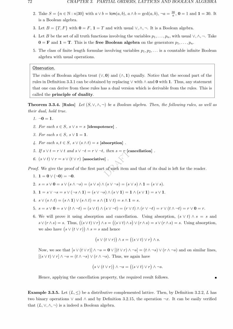
DRAFT


2. Take S = n ∈ N : n|30 with a∨ b = lcm(a, b), a∧ b = gcd(a, b), ¬a = 30a , 0 = 1 and 1 = 30. It

is a Boolean algebra.

3. Let B = T, F with 0 = F , 1 = T and with usual ∨,∧,¬. It is a Boolean algebra.

4. Let B be the set of all truth functions involving the variables p1, . . . , pn, with usual ∨,∧,¬. Take

0 = F and 1 = T. This is the free Boolean algebra on the generators p1, . . . , pn.

5. The class of finite length formulae involving variables p1, p2, . . . is a countable infinite Boolean

algebra with usual operations.

Observation.

The rules of Boolean algebra treat (∨,0) and (∧,1) equally. Notice that the second part of the

rules in Definition 3.3.1 can be obtained by replacing ∨ with ∧ and 0 with 1. Thus, any statement

that one can derive from these rules has a dual version which is derivable from the rules. This is

called the principle of duality.

Theorem 3.3.4. [Rules] Let (S,∨,∧,¬) be a Boolean algebra. Then, the following rules, as well as

their dual, hold true.

1. ¬0 = 1.

2. For each s ∈ S, s ∨ s = s [idempotence] .

3. For each s ∈ S, s ∨ 1 = 1.

4. For each s, t ∈ S, s ∨ (s ∧ t) = s [absorption] .

5. If s ∨ t = r ∨ t and s ∨ ¬t = r ∨ ¬t, then s = r [cancellation] .

6. (s ∨ t) ∨ r = s ∨ (t ∨ r) [associative] .

Proof. We give the proof of the first part of each item and that of its dual is left for the reader.

1. 1 = 0 ∨ (¬0) = ¬0.

2. s = s ∨ 0 = s ∨ (s ∧ ¬s) = (s ∨ s) ∧ (s ∨ ¬s) = (s ∨ s) ∧ 1 = (s ∨ s).3. 1 = s ∨ ¬s = s ∨ (¬s ∧ 1) = (s ∨ ¬s) ∧ (s ∨ 1) = 1 ∧ (s ∨ 1) = s ∨ 1.

4. s ∨ (s ∧ t) = (s ∧ 1) ∨ (s ∧ t) = s ∧ (1 ∨ t) = s ∧ 1 = s.

5. s = s ∨ 0 = s ∨ (t ∧ ¬t) = (s ∨ t) ∧ (s ∨ ¬t) = (r ∨ t) ∧ (r ∨ ¬t) = r ∨ (t ∧ ¬t) = r ∨ 0 = r.

6. We will prove it using absorption and cancellation. Using absorption, (s ∨ t) ∧ s = s and

s∨ (r∧ s) = s. Thus,((s∨ t)∨ r

)∧ s =

((s∨ t)∧ s

)∨ (r∧ s) = s∨ (r∧ s) = s. Using absorption,

we also have(s ∨ (t ∨ r)

)∧ s = s and hence(

s ∨ (t ∨ r))∧ s =

((s ∨ t) ∨ r

)∧ s.

Now, we see that [s ∨ (t ∨ r)] ∧ ¬s = 0 ∨ [(t ∨ r) ∧ ¬s] = (t ∧ ¬s) ∨ (r ∧ ¬s) and on similar lines,

[(s ∨ t) ∨ r] ∧ ¬s = (t ∧ ¬s) ∨ (r ∧ ¬s). Thus, we again have(s ∨ (t ∨ r)

)∧ ¬s =

((s ∨ t) ∨ r

)∧ ¬s.

Hence, applying the cancellation property, the required result follows.

Example 3.3.5. Let (L,≤) be a distributive complemented lattice. Then, by Definition 3.2.2, L has

two binary operations ∨ and ∧ and by Definition 3.2.15, the operation ¬x. It can be easily verified

that (L,∨,∧,¬) is a indeed a Boolean algebra.

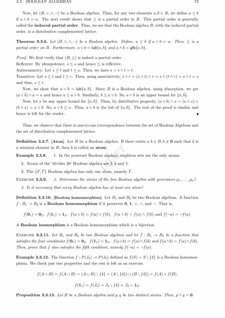
DRAFT


Now, let (B,∨,∧,¬) be a Boolean algebra. Then, for any two elements a, b ∈ B, we define a ≤ b

if a ∧ b = a. The next result shows that ≤ is a partial order in B. This partial order is generally

called the induced partial order. Thus, we see that the Boolean algebra B, with the induced partial

order, is a distributive complemented lattice.

Theorem 3.3.6. Let (B,∨,∧,¬) be a Boolean algebra. Define, a ≤ b if a ∧ b = a. Then, ≤ is a

partial order on B. Furthermore, a ∨ b = luba, b and a ∧ b = glba, b.

Proof. We first verify that (B,≤) is indeed a partial order.

Reflexive: By idempotence, s ≤ s and hence ≤ is reflexive.

Antisymmetry: Let s ≤ t and t ≤ s. Then, we have s = s ∧ t = t.

Transitive: Let s ≤ t and t ≤ r. Then, using associativity, s ∧ r = (s ∧ t) ∧ r = s ∧ (t ∧ r) = s ∧ t = s

and thus, s ≤ r.Now, we show that a ∨ b = luba, b. Since B is a Boolean algebra, using absorption, we get

(a ∨ b) ∧ a = a and hence a ≤ a ∨ b. Similarly, b ≤ a ∨ b. So, a ∨ b is an upper bound for a, b.Now, let x be any upper bound for a, b. Then, by distributive property, (a ∨ b) ∧ x = (a ∧ x) ∨

(b ∧ x) = a ∨ b. So, a ∨ b ≤ x. Thus, a ∨ b is the lub of a, b. The rest of the proof is similar and

hence is left for the reader.

Thus, we observe that there is one-to-one correspondence between the set of Boolean Algebras and

the set of distributive complemented lattice.

Definition 3.3.7. [Atom] Let B be a Boolean algebra. If there exists a b ∈ B, b 6= 0 such that b is

a minimal element in B, then b is called an atom.

Example 3.3.8. 1. In the powerset Boolean algebra, singleton sets are the only atoms.

2. Atoms of the ‘divides 30’ Boolean algebra are 2, 3 and 5.

3. The F, T Boolean algebra has only one atom, namely T .

Exercise 3.3.9. 1. Determine the atoms of the free Boolean algebra with generators p1, . . . , pn?

2. Is it necessary that every Boolean algebra has at least one atom?

Definition 3.3.10. [Boolean homomorphism] Let B1 and B2 be two Boolean algebras. A function

f : B1 → B2 is a Boolean homomorphism if it preserves 0, 1, ∨, ∧, and ¬. That is,

f(01) = 02, f(11) = 12, f(a ∨ b) = f(a) ∨ f(b), f(a ∧ b) = f(a) ∧ f(b), and f(¬a) = ¬f(a).

A Boolean isomorphism is a Boolean homomorphism which is a bijection.

Exercise 3.3.11. Let B1 and B2 be two Boolean algebras and let f : B1 → B2 be a function that

satisfies the four conditions f(01) = 02, f(11) = 12, f(a∨b) = f(a)∨f(b) and f(a∧b) = f(a)∧f(b).

Then, prove that f also satisfies the fifth condition, namely f(¬a) = ¬f(a).

Example 3.3.12. The function f : P (J4)→ P (J3) defined as f(S) = S \ 4 is a Boolean homomor-

phism. We check just two properties and the rest is left as an exercise.

f(A ∨B) = f(A ∪B) = (A ∪B) \ 4 = (A \ 4) ∪ (B \ 4) = f(A) ∨ f(B).

f(11) = f(J4) = J4 \ 4 = J3 = 12.

Proposition 3.3.13. Let B be a Boolean algebra and p, q be two distinct atoms. Then, p ∧ q = 0.

DRAFT


Proof. Suppose that p∧ q 6= 0. As p∧ q ≤ p and p is an atom, we must have p∧ q = p, i.e., q ≤ p. As

p 6= q and q is an atom, it follows that p cannot be an atom.

Proposition 3.3.14. Let B be a Boolean algebra with three distinct atoms p, q and r. Then, p ∨ q 6=p ∨ q ∨ r.

Proof. Let if possible p ∨ q = p ∨ q ∨ r. Then, we have

r = r ∨ 0 = r ∨ [(p ∨ q) ∧ ¬(p ∨ q)] = [r ∨ p ∨ q] ∧ [r ∨ ¬(p ∨ q)] = [p ∨ q] ∧ [r ∨ ¬(p ∨ q)]

= [(p ∨ q) ∧ r] ∨ [(p ∨ q) ∧ ¬(p ∨ q)] = (p ∨ q) ∧ r = (p ∧ r) ∨ (q ∧ r) = 0 ∨ 0 = 0,

a contradiction to r being an atom, i.e., r is nonzero.

Example 3.3.15. Let B be a Boolean algebra having distinct atoms A = p, q, r. Then, B has at

least 23 elements.

To show this, we define f : P(A)→ B by f(∅) = 0 and for S ⊆ A, f(S) =∨x∈S

x and claim that f

is a one-one function.

Suppose f(S) = f(T ). Then, f(S) = f(S) ∨ f(T ) = f(S ∪ T ). In view of Proposition 3.3.14, we

have S = S ∪ T , i.e., T ⊆ S. Similarly, as f(T ) = f(T ∪ S), we have S ⊆ T and hence S = T . Thus,

f is a one-one function. Therefore, f(S) is distinct, for each subset of A and thus B has at least 23

elements.

Theorem 3.3.16. Let B be a Boolean algebra having distinct atoms A = p, q, r, s. Let b ∈ B, b 6= 0.

Suppose that S = atoms x : x ≤ b = p, q, r. Then, b = p ∨ q ∨ r.

Proof. It is clear that p ∨ q ∨ r ≤ b. Suppose that p ∨ q ∨ r < b. Then,

b = b∧ [(p∨ q ∨ r)∨¬(p∨ q ∨ r)] = [b∧ (p∨ q ∨ r)]∨ [b∧¬(p∨ q ∨ r)] = (p∨ q ∨ r)∨ [b∧¬(p∨ q ∨ r)].

Therefore, the above equality implies that [b∧¬(p∨ q∨ r)] 6= 0. So, there is an atom, say x, such that

x ≤ b ∧ ¬(p ∨ q ∨ r). Thus, we have x ≤ b and x ≤ ¬(p ∨ q ∨ r).Notice that if x ≤ (p ∨ q ∨ r), then x ≤ 0, which is not possible. So, x 6= p, q, r is an atom in S, a

contradiction.

Theorem 3.3.17. [Representation] Let B be a finite Boolean algebra. Then, there exists a set X

such that B is isomorphic to P(X).

Proof. Put X = atoms of B. Note that X 6= ∅. Define f : B → P(X) by f(b) = atoms ≤ b. We

show that f is the required Boolean isomorphism.

Injection: Let b1 6= b2. Then, either b1 b2 or b2 b1. Without loss of generality, let b1 b2.

[Now imagine the power set Boolean algebra. Saying b1 b2 is the same as b1 * b2. In that case,

we have an element in b1 which is not in b2. That is, b1 ∩ bc2 6= ∅. That is, there is a singleton

subset of b1 ∩ bc2. This is exactly what we are aiming for, i.e., to prove that b1 ∧ ¬b2 6= 0.] Note that

b1 = b1 ∧ (b2 ∨ ¬b2) = (b1 ∧ b2) ∨ (b1 ∧ ¬b2). Also, the assumption b1 b2 implies b1 ∧ b2 6= b1 and

hence b1 ∧ ¬b2 6= 0. So, there exists an atom x ≤ (b1 ∧ ¬b2) and hence x = x ∧ b1 ∧ ¬b2. Therefore,

x ∧ b1 = (x ∧ b1 ∧ ¬b2) ∧ b1 = x ∧ b1 ∧ ¬b2 = x.

Thus, x ≤ b1. Similarly, x ≤ ¬b2. As x 6= 0, we cannot have x ≤ b2 (the condition x ≤ ¬b2 and x ≤ b2implies x ≤ b2 ∧ ¬b2 = 0). Thus, f(b1) 6= f(b2).

DRAFT


Surjection: Let A = x1, . . . , xk ⊆ X and put b = x1 ∨ · · · ∨ xk (if k = 0, then b = 0). Clearly,

A ⊆ f(b). Need to show: A = f(b). So, let y ∈ f(b), i.e., y is an atom in B and

y = y ∧ b = y ∧ (x1 ∨ · · · ∨ xk) = (y ∧ x1) ∨ · · · ∨ (y ∧ xk).

Since y 6= 0, by Proposition 3.3.13, it follows that y ∧ xi0 6= 0, for some i0 ∈ 1, 2, . . . , k. As xi0 and

y are atoms, we have y = y ∧ xi = xi and hence y ∈ A. Thus, f is a surjection.

Preserving 0,1: Clearly f(0) = ∅ and f(1) = X.

Preserving ∨,∧: By definition,

x ∈ f(b1 ∧ b2) ⇔ x ≤ b1 ∧ b2 ⇔ x ≤ b1 and x ≤ b2⇔ x ∈ f(b1) and x ∈ f(b2)⇔ x ∈ f(b1)∩ f(b2).

Now, let x ∈ f(b1 ∨ b2). Then, by definition, x = x ∧ (b1 ∨ b2) = (x ∧ b1) ∨ (x ∧ b2). So, there exists

i such that x ∧ bi 6= 0 (say, x ∧ b1). As, x is an atom, x ≤ b1 and hence x ∈ f(b1) ⊆ f(b1) ∪ f(b2).

Conversely, let x ∈ f(b1) ∪ f(b2). Without loss of generality, let x ∈ f(b1). Thus, x ≤ b1 and hence

x ≤ b1 ∨ b2 which in turn implies that x ∈ f(b1 ∨ b2).

As a direct corollary, we have the following result.

Corollary 3.3.18. Let B be a finite Boolean algebra having exactly k atoms. Then, B is isomorphic

to P(1, 2, . . . , k) and hence has exactly 2k elements.

Exercise 3.3.19. 1. Determine the number of elements in a finite Boolean algebra.

2. Supply a Boolean homomorphism f from P (J4) to P (J3) such that the image of P (J4) has 4

elements.

3. Prove/Disprove: The number of Boolean homomorphisms from P (J4) to P (J3) is less than the

number of lattice homomorphisms from P (J4) to P (J3).

4. Show that a lattice homomorphism on a Boolean algebra which preserves 0 and 1 is a Boolean

homomorphism.

5. Consider the class of all functions f : R→ π, e. Can we define some operations on this class

to make it a Boolean algebra?

6. Show that a finite Boolean algebra must have at least one atom. Is ‘finite’ necessary?

7. A positive integer is called square-free if it is not divisible by the square of a prime. Let

Bn = k ∈ N : k|n. For a, b ∈ Bn take the operations a ∨ b = lcm(a, b), a ∧ b = gcd(a, b) and

¬a = n/a. Show that Bn is a Boolean algebra if and only if n > 1 is square-free.

8. Show that the set of subsets of N which are either finite or have a finite complement is a countable

infinite Boolean algebra. Find the atoms. Is it isomorphic to the Boolean algebra of all finite

length formulae involving variables p1, p2, · · · ?9. Let B be a Boolean algebra and xi ∈ B, i = 1, 2, . . .. We know that, for each n ∈ N, the expres-

sion ‘n∨i=1

xi’ is meaningful in each Boolean algebra due to associativity. Is ‘∞∨i=1

xi’ necessarily a

meaningful expression?

10. Prove/Disprove: Let f : B1 → B2 be a Boolean homomorphism and a ∈ B1 be an atom. Then,

f(a) is an atom of B2.

11. Fill in the blank: The number of Boolean homomorphisms from P (J4) to P (J3) is .

12. Fill in the blank: The number of Boolean homomorphisms from P (J4) onto P (J3) is .

DRAFT


13. How many atoms does “divides 30030 Boolean algebra” has? How many elements does it have?

14. If B1 and B2 are Boolean algebras of size k (k > 100), then they must be isomorphic and there

must be more than k isomorphisms between them.

15. Give examples of two countably infinite non-isomorphic Boolean algebras.

16. Give examples of two uncountably infinite non-isomorphic Boolean algebras.

DRAFT

Chapter 4

Basic Counting

Discussion 4.0.1. In the previous chapters, we had learnt that two sets, say A and B, have the same

cardinality if there exists a one-one and onto function f : A → B. We also learnt the following two

rules of counting which play a basic role in the development of this subject.

1. [Multiplication rule] If a task has n compulsory parts, say A1, A2, . . . , An and the i-th part can

be completed in mi = |Ai| ways, i = 1, . . . , n, then the task can be completed in m1m2 · · ·mn

ways. In mathematical terms,

|A1 ×A2 × · · · ×An| = |A1| · |A2| · · · · · |An|.

2. [Addition rule] If a task consists of n alternative parts, say A1, A2, . . . , An, and the ith part can

be done in |Ai| = mi ways, i = 1, . . . , n, then the task can be completed in m1 +m2 + · · ·+mn

ways. In mathematical terms,

|A1 ∪A2 ∪ · · · ∪An| = |A1|+ |A2|+ · · ·+ |An|, whenever Ai ∩Aj 6= ∅, 1 ≤ i < j ≤ n.

Example 4.0.2. 1. How many three digit natural numbers can be formed using digits 0, 1, · · · , 9?

Identify the number of parts in the task and the type of the parts (compulsory or alternative).

Which rule applies here?

Ans: The task has three compulsory parts. Part 1: choose a digit for the leftmost place. Part 2:

choose a digit for the middle place. Part 3: choose a digit for the rightmost place.

Multiplication rule applies. Ans: 900.

2. How many three digit natural numbers with distinct digits can be formed using digits 1, · · · , 9such that each digit is odd or each digit is even? Identify the number of parts in the task and

the type of the parts (compulsory or alternative). Which rule applies here?

Ans: The task has two alternative parts. Part 1: form a three digit number with distinct

numbers from 1, 3, 5, 7, 9 using the odd digits. Part 2: form a three digit number with distinct

numbers from 2, 4, 6, 8 using the even digits. Observe that Part 1 is a task having three

compulsory subparts. In view of 4.0.2, we see that Part 1 can be done in 60 ways. Part 2 is a

task having three compulsory subparts. In view of 4.0.2, we see that Part 2 can be done in 24

ways. Since our task has alternative parts, addition rule applies. Ans: 84.

Definition 4.0.3. We use the notation n! = 1 · 2 · · · · · n. By convention, we take 0! = 1.

77

DRAFT

78 CHAPTER 4. BASIC COUNTING

4.1 Permutations and Combinations

Definition 4.1.1. An r-sequence of elements of X is a sequence of length r with elements from X.

This may be viewed as a word of length r with alphabets from X or as a function f : 1, 2, . . . , r → X.

We write ‘an r-sequence of X’ to mean ‘an r-sequence of elements of X’.

Theorem 4.1.2. The number of r-sequences of 1, 2, . . . , n is nr.

Proof. Here the task has r compulsory parts. Choose the first element of the sequence, the second

element and so on.

Exercise 4.1.3. 1. In how many ways can r distinguishable/distinct balls be put into n dis-

tinguishable/distinct boxes?

2. How many distinct ways are there to make a 5 letter word using the ENGLISH alphabet

(a) with no restriction?

(b) with ONLY consonants?

(c) with ONLY vowels?

(d) with a consonant as the first letter and a vowel as the second letter?

(e) if the vowels appear only at odd positions?

3. Determine the total number of possible outcomes if

(a) two coins are tossed?

(b) a coin and a die are tossed?

(c) two dice are tossed?

(d) three dice are tossed?

(e) k dice are tossed, where k ∈ N?

(f) five coins are tossed?

4. How many 5-letter words using only A’s, B’s, C’s, and D’s are there that do not contain the

word “CAD”?

Definition 4.1.4. [r-permutation, n-set] By an n-set, we mean a set containing n elements. An

r-permutation of an n-set S is an arrangement of r distinct elements of S in a row. An r-permutation

may be viewed as a one-one mapping f : 1, 2, . . . , r → S. An n-permutation of an n-set is simply

called a permutation.

Example 4.1.5. How many one-one maps f : 1, 2, 3, 4 → A = A,B, . . . , Z are there?

Ans: The task has 4 compulsory parts: select f(1), select f(2), select f(3) and select f(4). Note

that f(2) cannot be f(1), f(3) cannot be f(1) or f(2) and so on. Now apply the multiplication rule.

Ans: 26 · 25 · 24 · 23 = 26!22! .

Theorem 4.1.6. [Number of r-permutations] The number of r-permutation of an n-set S is

P (n, r) = n!(n−r)! .

Proof. Let us view an r-permutation as a one-one map from f : 1, 2, . . . , r → S. Here the task

has r compulsory tasks: select f(1), select f(2), . . ., select f(r) with the condition, for 2 ≤ k ≤ r,

f(k) 6∈ f(1), f(2), . . . , f(k − 1). Multiplication rule applies. Hence, the number of r-permutations

equals n(n− 1) · · · (n− r + 1) = n!(n−r)! .

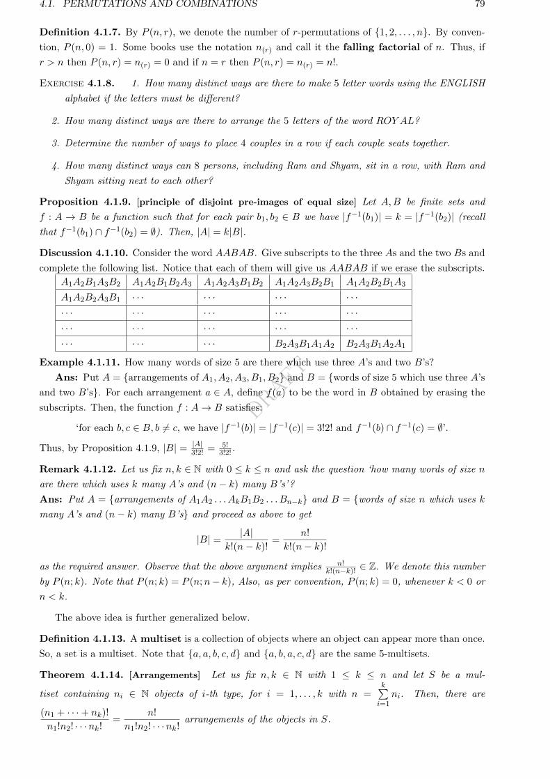
DRAFT

4.1. PERMUTATIONS AND COMBINATIONS 79

Definition 4.1.7. By P (n, r), we denote the number of r-permutations of 1, 2, . . . , n. By conven-

tion, P (n, 0) = 1. Some books use the notation n(r) and call it the falling factorial of n. Thus, if

r > n then P (n, r) = n(r) = 0 and if n = r then P (n, r) = n(r) = n!.

Exercise 4.1.8. 1. How many distinct ways are there to make 5 letter words using the ENGLISH

alphabet if the letters must be different?

2. How many distinct ways are there to arrange the 5 letters of the word ROY AL?

3. Determine the number of ways to place 4 couples in a row if each couple seats together.

4. How many distinct ways can 8 persons, including Ram and Shyam, sit in a row, with Ram and

Shyam sitting next to each other?

Proposition 4.1.9. [principle of disjoint pre-images of equal size] Let A,B be finite sets and

f : A → B be a function such that for each pair b1, b2 ∈ B we have |f−1(b1)| = k = |f−1(b2)| (recall

that f−1(b1) ∩ f−1(b2) = ∅). Then, |A| = k|B|.

Discussion 4.1.10. Consider the word AABAB. Give subscripts to the three As and the two Bs and

complete the following list. Notice that each of them will give us AABAB if we erase the subscripts.

A1A2B1A3B2 A1A2B1B2A3 A1A2A3B1B2 A1A2A3B2B1 A1A2B2B1A3

A1A2B2A3B1 · · · · · · · · · · · ·· · · · · · · · · · · · · · ·· · · · · · · · · · · · · · ·· · · · · · · · · B2A3B1A1A2 B2A3B1A2A1

Example 4.1.11. How many words of size 5 are there which use three A’s and two B’s?

Ans: Put A = arrangements of A1, A2, A3, B1, B2 and B = words of size 5 which use three A’s

and two B’s. For each arrangement a ∈ A, define f(a) to be the word in B obtained by erasing the

subscripts. Then, the function f : A→ B satisfies:

‘for each b, c ∈ B, b 6= c, we have |f−1(b)| = |f−1(c)| = 3!2! and f−1(b) ∩ f−1(c) = ∅’.

Thus, by Proposition 4.1.9, |B| = |A|3!2! = 5!

3!2! .

Remark 4.1.12. Let us fix n, k ∈ N with 0 ≤ k ≤ n and ask the question ‘how many words of size n

are there which uses k many A’s and (n− k) many B’s’?

Ans: Put A = arrangements of A1A2 . . . AkB1B2 . . . Bn−k and B = words of size n which uses k

many A’s and (n− k) many B’s and proceed as above to get

|B| = |A|k!(n− k)!

=n!

k!(n− k)!

as the required answer. Observe that the above argument implies n!k!(n−k)! ∈ Z. We denote this number

by P (n; k). Note that P (n; k) = P (n;n− k), Also, as per convention, P (n; k) = 0, whenever k < 0 or

n < k.

The above idea is further generalized below.

Definition 4.1.13. A multiset is a collection of objects where an object can appear more than once.

So, a set is a multiset. Note that a, a, b, c, d and a, b, a, c, d are the same 5-multisets.

Theorem 4.1.14. [Arrangements] Let us fix n, k ∈ N with 1 ≤ k ≤ n and let S be a mul-

tiset containing ni ∈ N objects of i-th type, for i = 1, . . . , k with n =k∑i=1

ni. Then, there are

(n1 + · · ·+ nk)!

n1!n2! · · ·nk!=

n!

n1!n2! · · ·nk!arrangements of the objects in S.

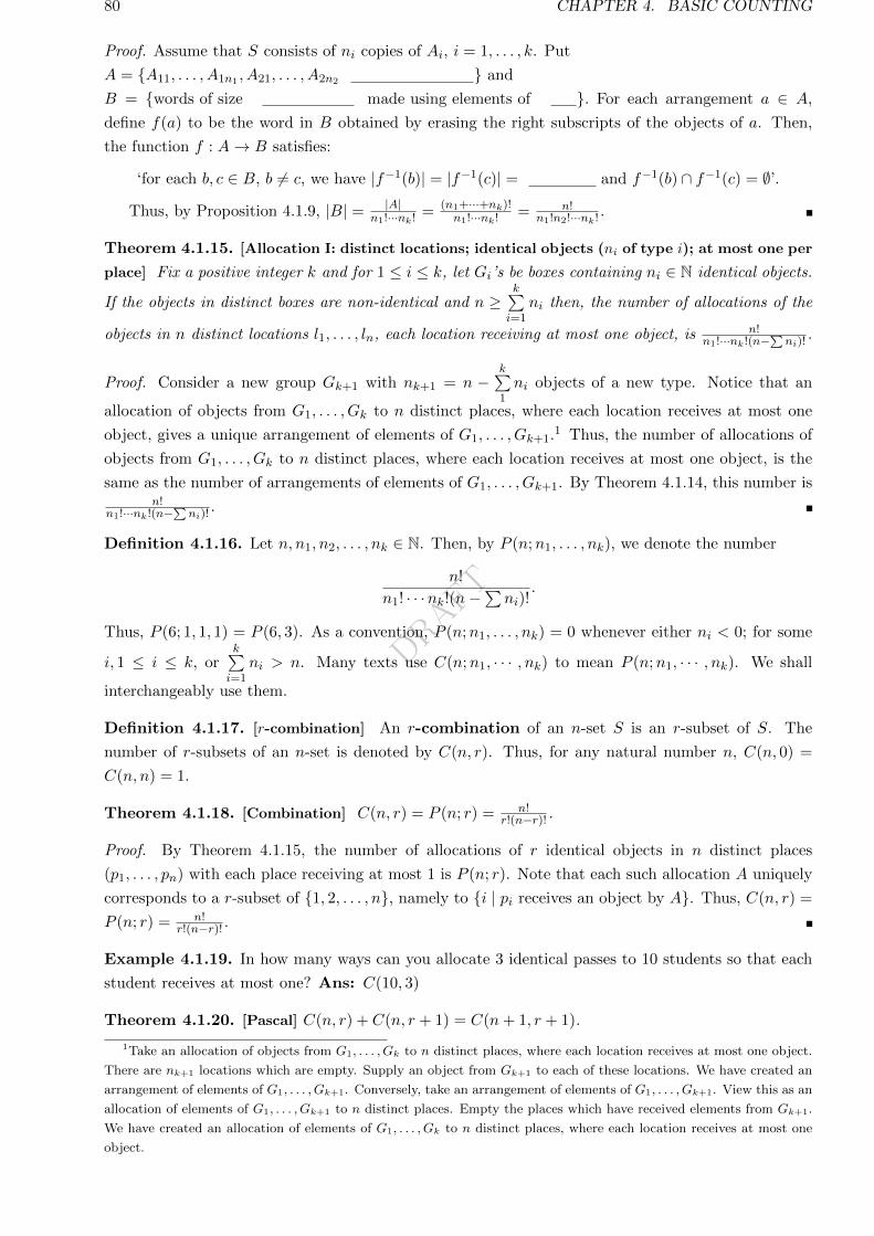
DRAFT


Proof. Assume that S consists of ni copies of Ai, i = 1, . . . , k. Put

A = A11, . . . , A1n1 , A21, . . . , A2n2 and

B = words of size made using elements of . For each arrangement a ∈ A,

define f(a) to be the word in B obtained by erasing the right subscripts of the objects of a. Then,

the function f : A→ B satisfies:

‘for each b, c ∈ B, b 6= c, we have |f−1(b)| = |f−1(c)| = and f−1(b) ∩ f−1(c) = ∅’.

Thus, by Proposition 4.1.9, |B| = |A|n1!···nk! = (n1+···+nk)!

n1!···nk! = n!n1!n2!···nk! .

Theorem 4.1.15. [Allocation I: distinct locations; identical objects (ni of type i); at most one per

place] Fix a positive integer k and for 1 ≤ i ≤ k, let Gi’s be boxes containing ni ∈ N identical objects.

If the objects in distinct boxes are non-identical and n ≥k∑i=1

ni then, the number of allocations of the

objects in n distinct locations l1, . . . , ln, each location receiving at most one object, is n!n1!···nk!(n−

∑ni)!

.

Proof. Consider a new group Gk+1 with nk+1 = n −k∑1ni objects of a new type. Notice that an

allocation of objects from G1, . . . , Gk to n distinct places, where each location receives at most one

object, gives a unique arrangement of elements of G1, . . . , Gk+1.1 Thus, the number of allocations of

objects from G1, . . . , Gk to n distinct places, where each location receives at most one object, is the

same as the number of arrangements of elements of G1, . . . , Gk+1. By Theorem 4.1.14, this number isn!

n1!···nk!(n−∑ni)!

.

Definition 4.1.16. Let n, n1, n2, . . . , nk ∈ N. Then, by P (n;n1, . . . , nk), we denote the number

n!

n1! · · ·nk!(n−∑ni)!

.

Thus, P (6; 1, 1, 1) = P (6, 3). As a convention, P (n;n1, . . . , nk) = 0 whenever either ni < 0; for some

i, 1 ≤ i ≤ k, ork∑i=1

ni > n. Many texts use C(n;n1, · · · , nk) to mean P (n;n1, · · · , nk). We shall

interchangeably use them.

Definition 4.1.17. [r-combination] An r-combination of an n-set S is an r-subset of S. The

number of r-subsets of an n-set is denoted by C(n, r). Thus, for any natural number n, C(n, 0) =

C(n, n) = 1.

Theorem 4.1.18. [Combination] C(n, r) = P (n; r) = n!r!(n−r)! .

Proof. By Theorem 4.1.15, the number of allocations of r identical objects in n distinct places

(p1, . . . , pn) with each place receiving at most 1 is P (n; r). Note that each such allocation A uniquely

corresponds to a r-subset of 1, 2, . . . , n, namely to i | pi receives an object by A. Thus, C(n, r) =

P (n; r) = n!r!(n−r)! .

Example 4.1.19. In how many ways can you allocate 3 identical passes to 10 students so that each

student receives at most one? Ans: C(10, 3)

Theorem 4.1.20. [Pascal] C(n, r) + C(n, r + 1) = C(n+ 1, r + 1).

1Take an allocation of objects from G1, . . . , Gk to n distinct places, where each location receives at most one object.

There are nk+1 locations which are empty. Supply an object from Gk+1 to each of these locations. We have created an

arrangement of elements of G1, . . . , Gk+1. Conversely, take an arrangement of elements of G1, . . . , Gk+1. View this as an

allocation of elements of G1, . . . , Gk+1 to n distinct places. Empty the places which have received elements from Gk+1.

We have created an allocation of elements of G1, . . . , Gk to n distinct places, where each location receives at most one

object.

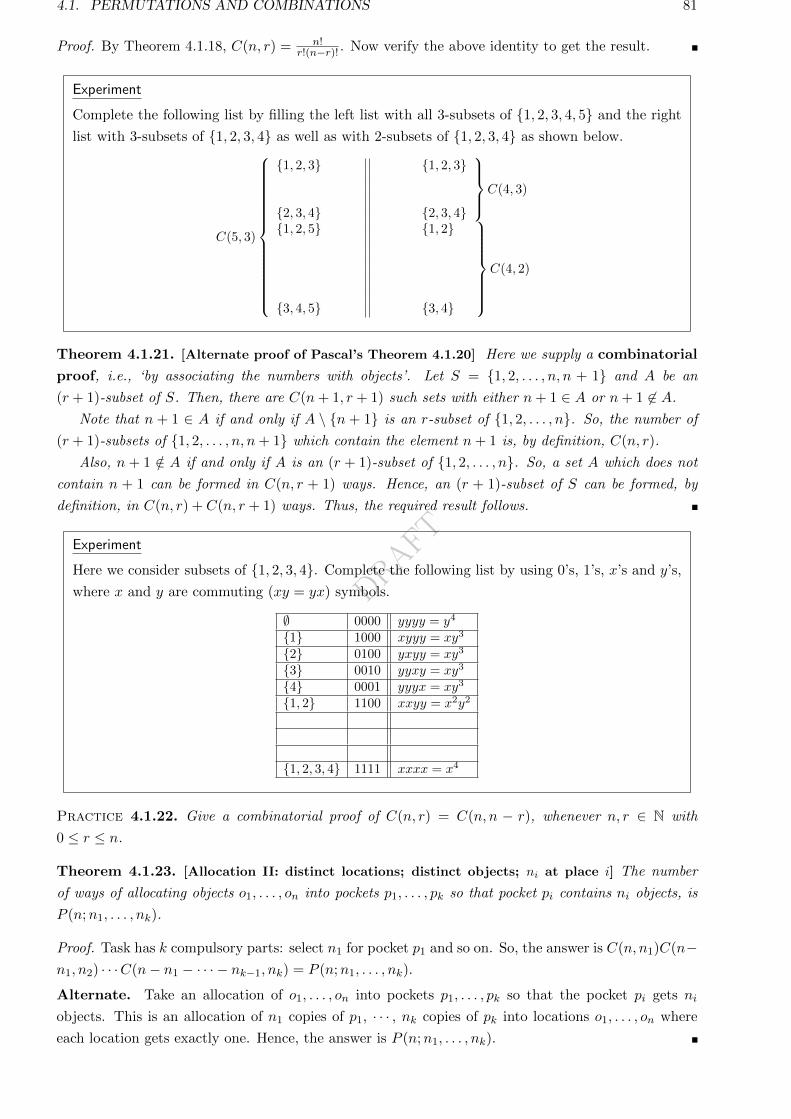
DRAFT


Proof. By Theorem 4.1.18, C(n, r) = n!r!(n−r)! . Now verify the above identity to get the result.

Experiment

Complete the following list by filling the left list with all 3-subsets of 1, 2, 3, 4, 5 and the right

list with 3-subsets of 1, 2, 3, 4 as well as with 2-subsets of 1, 2, 3, 4 as shown below.

C(5, 3)

1, 2, 3

2, 3, 41, 2, 5

3, 4, 5

1, 2, 3

2, 3, 4

C(4, 3)

1, 2

3, 4

C(4, 2)

Theorem 4.1.21. [Alternate proof of Pascal’s Theorem 4.1.20] Here we supply a combinatorial

proof, i.e., ‘by associating the numbers with objects’. Let S = 1, 2, . . . , n, n + 1 and A be an

(r + 1)-subset of S. Then, there are C(n+ 1, r + 1) such sets with either n+ 1 ∈ A or n+ 1 6∈ A.

Note that n + 1 ∈ A if and only if A \ n + 1 is an r-subset of 1, 2, . . . , n. So, the number of

(r + 1)-subsets of 1, 2, . . . , n, n+ 1 which contain the element n+ 1 is, by definition, C(n, r).

Also, n + 1 /∈ A if and only if A is an (r + 1)-subset of 1, 2, . . . , n. So, a set A which does not

contain n + 1 can be formed in C(n, r + 1) ways. Hence, an (r + 1)-subset of S can be formed, by

definition, in C(n, r) + C(n, r + 1) ways. Thus, the required result follows.

Experiment

Here we consider subsets of 1, 2, 3, 4. Complete the following list by using 0’s, 1’s, x’s and y’s,

where x and y are commuting (xy = yx) symbols.

∅ 0000 yyyy = y4

1 1000 xyyy = xy3

2 0100 yxyy = xy3

3 0010 yyxy = xy3

4 0001 yyyx = xy3

1, 2 1100 xxyy = x2y2

1, 2, 3, 4 1111 xxxx = x4

Practice 4.1.22. Give a combinatorial proof of C(n, r) = C(n, n − r), whenever n, r ∈ N with

0 ≤ r ≤ n.

Theorem 4.1.23. [Allocation II: distinct locations; distinct objects; ni at place i] The number

of ways of allocating objects o1, . . . , on into pockets p1, . . . , pk so that pocket pi contains ni objects, is

P (n;n1, . . . , nk).

Proof. Task has k compulsory parts: select n1 for pocket p1 and so on. So, the answer is C(n, n1)C(n−n1, n2) · · ·C(n− n1 − · · · − nk−1, nk) = P (n;n1, . . . , nk).

Alternate. Take an allocation of o1, . . . , on into pockets p1, . . . , pk so that the pocket pi gets ni

objects. This is an allocation of n1 copies of p1, · · · , nk copies of pk into locations o1, . . . , on where

each location gets exactly one. Hence, the answer is P (n;n1, . . . , nk).

DRAFT


Exercise 4.1.24. 1. In a class there are 17 girls and 20 boys. A committee of 5 students is to be

formed to represent the class.

(a) Determine the number of ways of forming the committee consisting of 5 students.

(b) Suppose the committee also needs to choose two different people from among themselves,

who will act as “spokesperson” and “treasurer”. In this case, determine the number of ways

of forming a committee consisting of 5 students. Note that two committees are different if

i. either the members are different, or

ii. even if the members are the same, they have different students as spokesperson and/or

treasurer.

(c) Due to certain restrictions, it was felt that the committee should have at least 3 girls. In

this case, determine the number of ways of forming the committee consisting of 5 students

(no one is to be designated as spokesperson and/or treasurer).

2. Combinatorially prove the following identities:

(a) kC(n, k) = nC(n− 1, k − 1).

(b) [Newton’s Identity] : C(n, r)C(r, k) = C(n, k)C(n− k, r − k).

(c) C(n, r) = C(r, r)C(n− r, 0) + C(r, r − 1)C(n− r, 1) + · · ·+ C(r, 0)C(n− r, r).(d) C(n, 0)2 + C(n, 1)2 + · · ·+ C(n, n)2 = C(2n, n).

3. Determine the number of ways of selecting a committee of m people from a group consisting of

n1 women and n2 men, with n1 + n2 ≥ m.

4. Determine the number of ways of arranging the letters of the word

(a) ABRACADABARAARCADA.

(b) KAGARTHALAMNAGARTHALAM .

5. How many anagrams of MISSISSIPPI are there so that no two S are adjacent?

6. How many rectangles are there in an n× n square? How many squares are there?

7. Show that a product of n consecutive natural numbers is always divisible by n!.

8. Show that (m!)n divides (mn)!.

9. If n points are placed on the circumference of a circle and all the lines connecting them are

joined, what is the largest number of points of intersection of these lines inside the circle that

can be obtained?

10. Prove that C(pn, pn− n) is a multiple of p in two ways. Hint: Newton’s identity.

11. How many ways are there to form the word MATHEMATICIAN starting from any side and

moving only in horizontal or vertical directions?M

M A MM A T A M

M A T H T A MM A T H E H T A M

M A T H E M E H T A MM A T H E M A M E H T A M

M A T H E M A T A M E H T A MM A T H E M A T I T A M E H T A M

M A T H E M A T I C I T A M E H T A MM A T H E M A T I C I C I T A M E H T A M

M A T H E M A T I C I A I C I T A M E H T A MM A T H E M A T I C I A N A I C I T A M E H T A M

12. (a) In how many ways can one arrange n different books in m different boxes kept in a row, if

books inside the boxes are also kept in a row?

(b) What if no box can be empty?

13. Prove by induction that 2n|(n+ 1) · · · (2n).

DRAFT


4.1.1 Multinomial theorem

Definition 4.1.25. Let x, y and z be commuting symbols. Then, by an algebraic expansion1 of

(x+ y+ z)n we mean an expansion where each term is of the form αxiyjzk so that two terms differ in

the degree of at least one of x, y, or z. By a word expansion2 of (x+ y+ z)n we mean an expansion

where each term is a word of length n using symbols x, y, z. Expansions for (x1 + · · ·+xr)n, whenever

xi’s are commuting symbols, may be defined in a similar way.

Example 4.1.26. 1. x3 + 3xy2 + y3 + 3yx2 is an algebraic expansion of (x+ y)3, where as xxx+

xxy + xyx+ xyy + yxx+ yxy + yyx+ yyy is a word expansion of (x+ y)3.

2. Take the word expansion of (X+Y +Z)9. A term with exactly two X’s and exactly three Y ’s is

nothing but an arrangement of two X’s, three Y ’s and four Z’s. So, the coefficient of X2Y 3Z4

in the algebraic expansion of (X + Y + Z)9 is P (9; 2, 3, 4).

3. Consider (x+ y + z)n = (x+ y + z) · (x+ y + z) · · · · · (x+ y + z)︸︷︷︸n times

. Then, in this expression, we

need to choose, say

(a) i places from the n possible places for x (i ≥ 0),

(b) j places from the remaining n− i places for y (j ≥ 0), and

(c) the n− i− j left out places for z (with n− i− j ≥ 0).

Thus, we get

(x+ y + z)n =∑

i,j≥0,i+j≤nC(n, i)C(n− i, j)xiyjzn−i−j =

∑i,j≥0,i+j≤n

P (n; i, j)xiyjzn−i−j .

Theorem 4.1.27. [Multinomial Theorem] Fix a positive integer n and let x1, x2, . . . , xn be a col-

lection of commuting symbols. Then, for n = n1 + · · · + nk, the coefficient of xn11 x

n22 · · ·xnkk in the

algebraic expansion of (x1 + · · ·+ xk)n is P (n;n1, · · · , nk). So

(x1 + · · ·+ xk)n =

∑n1, . . . , nk ≥ 0n1 + · · ·+ nk = n

P (n;n1, · · · , nk) xn11 · · ·xnkk .

Proof. The proof is left as an exercise for the reader.

As a special case, we have the famous binomial theorem.

Corollary 4.1.28. [Binomial Theorem] (x+ y)n =n∑k=0

C(n, k)xn−kyk. !!

Example 4.1.29. Form words of size 5 using letters from ‘MATHEMATICIAN’ (including multiplic-

ity, that is, you may use M at most twice). How many are there?

Ans:∑

k1+···+k8=5

k1≤2,k2≤3,k3≤2,k4≤1,k5≤1,k6≤2,k7≤1,k8≤1

C(5; k1, · · · , k8).

Exercise 4.1.30. 1. Show that |P(1, 2, . . . , n)| = 2n in the following ways.

(a) By using Binomial Theorem.

(b) By using ‘select a subset is a task with n compulsory parts’.

(c) By associating a subset with a 0-1 string of length n and evaluating their values in base-2.

(d) Arguing in the line of ‘a subset of 1, 2, . . . , n, n+1 either contains n+1 or not’ and using

induction.

1Nonstandard notion2Nonstandard notion

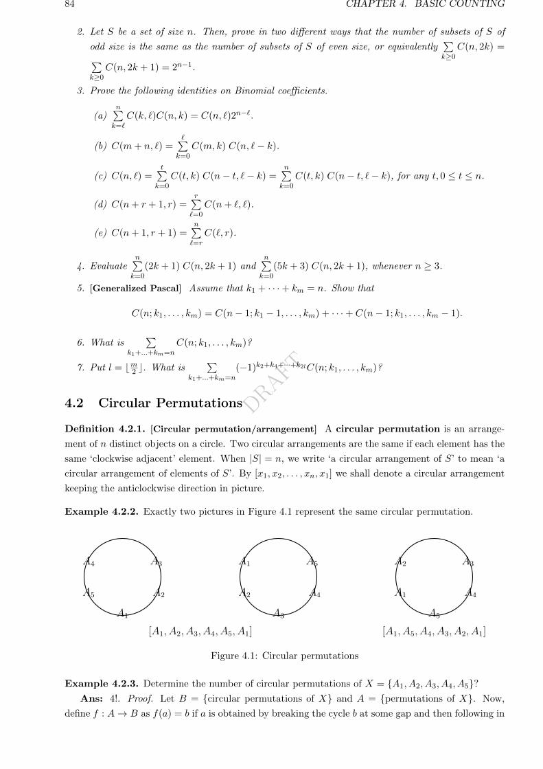
DRAFT


2. Let S be a set of size n. Then, prove in two different ways that the number of subsets of S of

odd size is the same as the number of subsets of S of even size, or equivalently∑k≥0

C(n, 2k) =∑k≥0

C(n, 2k + 1) = 2n−1.

3. Prove the following identities on Binomial coefficients.

(a)n∑k=`

C(k, `)C(n, k) = C(n, `)2n−`.

(b) C(m+ n, `) =∑k=0

C(m, k) C(n, `− k).

(c) C(n, `) =t∑

k=0

C(t, k) C(n− t, `− k) =n∑k=0

C(t, k) C(n− t, `− k), for any t, 0 ≤ t ≤ n.

(d) C(n+ r + 1, r) =r∑=0

C(n+ `, `).

(e) C(n+ 1, r + 1) =n∑=r

C(`, r).

4. Evaluaten∑k=0

(2k + 1) C(n, 2k + 1) andn∑k=0

(5k + 3) C(n, 2k + 1), whenever n ≥ 3.

5. [Generalized Pascal] Assume that k1 + · · ·+ km = n. Show that

C(n; k1, . . . , km) = C(n− 1; k1 − 1, . . . , km) + · · ·+ C(n− 1; k1, . . . , km − 1).

6. What is∑

k1+...+km=n

C(n; k1, . . . , km)?

7. Put l = bm2 c. What is∑

k1+...+km=n

(−1)k2+k4+···+k2lC(n; k1, . . . , km)?

4.2 Circular Permutations

Definition 4.2.1. [Circular permutation/arrangement] A circular permutation is an arrange-

ment of n distinct objects on a circle. Two circular arrangements are the same if each element has the

same ‘clockwise adjacent’ element. When |S| = n, we write ‘a circular arrangement of S’ to mean ‘a

circular arrangement of elements of S’. By [x1, x2, . . . , xn, x1] we shall denote a circular arrangement

keeping the anticlockwise direction in picture.

Example 4.2.2. Exactly two pictures in Figure 4.1 represent the same circular permutation.

A1

A2

A3A4

A5

[A1, A2, A3, A4, A5, A1]

A3

A4

A5A1

A2

A5

A4

A3A2

A1

[A1, A5, A4, A3, A2, A1]

1

Figure 4.1: Circular permutations

Example 4.2.3. Determine the number of circular permutations of X = A1, A2, A3, A4, A5?Ans: 4!. Proof. Let B = circular permutations of X and A = permutations of X. Now,

define f : A→ B as f(a) = b if a is obtained by breaking the cycle b at some gap and then following in

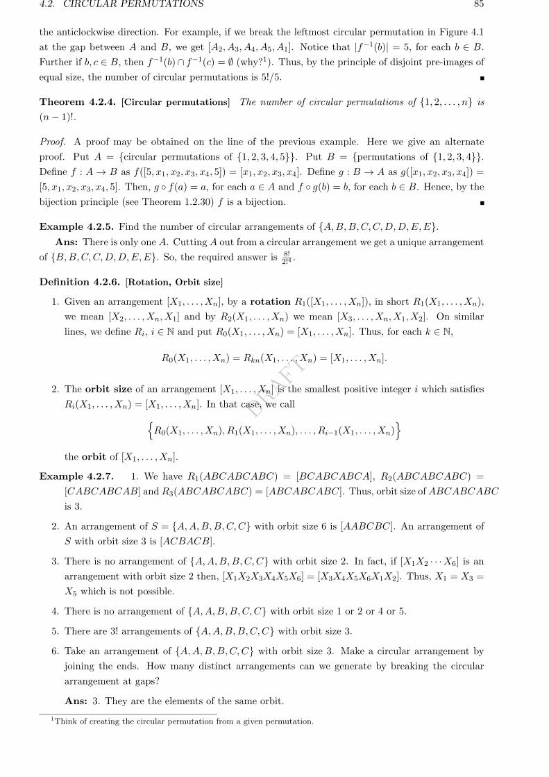
DRAFT

4.2. CIRCULAR PERMUTATIONS 85

the anticlockwise direction. For example, if we break the leftmost circular permutation in Figure 4.1

at the gap between A and B, we get [A2, A3, A4, A5, A1]. Notice that |f−1(b)| = 5, for each b ∈ B.

Further if b, c ∈ B, then f−1(b)∩ f−1(c) = ∅ (why?1). Thus, by the principle of disjoint pre-images of

equal size, the number of circular permutations is 5!/5.

Theorem 4.2.4. [Circular permutations] The number of circular permutations of 1, 2, . . . , n is

(n− 1)!.

Proof. A proof may be obtained on the line of the previous example. Here we give an alternate

proof. Put A = circular permutations of 1, 2, 3, 4, 5. Put B = permutations of 1, 2, 3, 4.Define f : A → B as f([5, x1, x2, x3, x4, 5]) = [x1, x2, x3, x4]. Define g : B → A as g([x1, x2, x3, x4]) =

[5, x1, x2, x3, x4, 5]. Then, g f(a) = a, for each a ∈ A and f g(b) = b, for each b ∈ B. Hence, by the

bijection principle (see Theorem 1.2.30) f is a bijection.

Example 4.2.5. Find the number of circular arrangements of A,B,B,C,C,D,D,E,E.Ans: There is only one A. Cutting A out from a circular arrangement we get a unique arrangement

of B,B,C,C,D,D,E,E. So, the required answer is 8!2!4

.

Definition 4.2.6. [Rotation, Orbit size]

1. Given an arrangement [X1, . . . , Xn], by a rotation R1([X1, . . . , Xn]), in short R1(X1, . . . , Xn),

we mean [X2, . . . , Xn, X1] and by R2(X1, . . . , Xn) we mean [X3, . . . , Xn, X1, X2]. On similar

lines, we define Ri, i ∈ N and put R0(X1, . . . , Xn) = [X1, . . . , Xn]. Thus, for each k ∈ N,

R0(X1, . . . , Xn) = Rkn(X1, . . . , Xn) = [X1, . . . , Xn].

2. The orbit size of an arrangement [X1, . . . , Xn] is the smallest positive integer i which satisfies

Ri(X1, . . . , Xn) = [X1, . . . , Xn]. In that case, we callR0(X1, . . . , Xn), R1(X1, . . . , Xn), . . . , Ri−1(X1, . . . , Xn)

the orbit of [X1, . . . , Xn].

Example 4.2.7. 1. We have R1(ABCABCABC) = [BCABCABCA], R2(ABCABCABC) =

[CABCABCAB] andR3(ABCABCABC) = [ABCABCABC]. Thus, orbit size ofABCABCABC

is 3.

2. An arrangement of S = A,A,B,B,C,C with orbit size 6 is [AABCBC]. An arrangement of

S with orbit size 3 is [ACBACB].

3. There is no arrangement of A,A,B,B,C,C with orbit size 2. In fact, if [X1X2 · · ·X6] is an

arrangement with orbit size 2 then, [X1X2X3X4X5X6] = [X3X4X5X6X1X2]. Thus, X1 = X3 =

X5 which is not possible.

4. There is no arrangement of A,A,B,B,C,C with orbit size 1 or 2 or 4 or 5.

5. There are 3! arrangements of A,A,B,B,C,C with orbit size 3.

6. Take an arrangement of A,A,B,B,C,C with orbit size 3. Make a circular arrangement by

joining the ends. How many distinct arrangements can we generate by breaking the circular

arrangement at gaps?

Ans: 3. They are the elements of the same orbit.

1Think of creating the circular permutation from a given permutation.

DRAFT


7. Take an arrangement of A,A,B,B,C,C with orbit size 6. Make a circular arrangement by

joining the ends. How many distinct arrangements can we generate by breaking the circular

arrangement at gaps?

Ans: 6. They are the elements of the same orbit.

8. Take an arrangement of n elements with orbit size k. Make a circular arrangement by joining the

ends. How many distinct arrangements can we generate by breaking the circular arrangement

at gaps?

Ans: k. They are the elements of the same orbit.

9. If we take the set of all arrangements of a finite multiset and group them into orbits (notice that

each orbit gives us exactly one circular arrangement), then the number of orbits is the number

of circular arrangements.

Example 4.2.8. Find the number of circular arrangements of S = A,A,B,B,C,C,D,D,E,E.Ans: There are two types of arrangements of S: one of orbit size 10 and the other of orbit

size 5. The number of arrangements of S with orbit size 5 is 5!. So, they can generate 4! distinct

circular arrangements. The number of arrangements of S with orbit size 10 is 10!2!2!2!2!2! − 5!. Hence,

they can generate 10!2!2!2!2!2!10 − 5!

10 distinct circular arrangements. Thus, the total number of circular

arrangements is 4! + 10!2!2!2!2!2!10 − 5!

10 .

Example 4.2.9. Suppose, we are given an arrangement [X1, . . . , X10] of five A’s and five B’s. Can it

have an orbit size 3?

Ans: No. To see this assume that it’s orbit size is 3. Then,

[X1, . . . , X10] = R3(X1, . . . , X10) = R6(X1, . . . , X10) = R9(X1, . . . , X10) = R2(X1, . . . , X10).

Since 3 was the least positive integer with R3(X1, . . . , X10) = [X1, . . . , X10], we arrive at a contradic-

tion. Hence, the orbit size cannot be 3.

Proposition 4.2.10. The orbit size of an arrangement of an n-multiset is a divisor of n.

Proof. Suppose, the orbit size of [X1, . . . , Xn] is k and n = kp+ r, for some r, 0 < r < k. Then,

Rk(X1, . . . , Xn) = R2k(X1, . . . , Xn) = · · · = Rkp(X1, . . . , Xn) = Rk−r(X1, . . . , Xn).

Thus, Rk−r(X1, . . . , Xn) = [X1, . . . , Xn], contradicting the minimality of k. Hence, a contradiction

and therefore r = 0. Or equivalently, k divides n.

Proposition 4.2.11. Let S1 = Pi1 , Pi2 , . . . , Pik and S2 = Pj1 , Pj2 , . . . , Pjl be any two orbits of

certain arrangements of an n-multiset. Then, either S1 ∩ S2 = ∅ or S1 = S2.

Proof. If S1 ∩S2 = ∅, then there is nothing to prove. So, let there exists an arrangement Pt ∈ S1 ∩S2.Then, by definition, there exist rotations R1 and R2 such that R1(Pi1) = Pt and R2(Pj1) = Pt. Thus,

R−12 (Pt) = Pj1 and hence R−12 (R1(Pi1)) = R−12 (Pt) = Pj1 . Therefore, we see that the arrangement

Pj1 ∈ S1 and hence S2 ⊆ S1. A similar argument implies that S1 ⊆ S2 and hence S1 = S2.

Definition 4.2.12. [Binary operation] Let [X1, . . . , Xn] and [Y1, . . . , Yn] be two arrangements of an

n-multiset. Then, in the remainder of this section,

1. we shall consider expressions like [X1, . . . , Xn] + [Y1, . . . , Yn].

2. by [Ri +Rj ](X1, . . . , Xn), we mean the expression Ri(X1, . . . , Xn) +Rj(X1, . . . , Xn).

3. by Ri([X1, . . . , Xn] + [Y1, . . . , Yn]) we denote the expression Ri(X1, . . . , Xn) +Ri(Y1, . . . , Yn).

DRAFT

4.2. CIRCULAR PERMUTATIONS 87

Example 4.2.13. Think of all arrangements P1, . . . , Pn, n = 6!3!3! , of three A’s and three B’s. How

many copies of [ABCABC] are there in [R0 + · · ·+R5](P1 + · · ·+ Pn)?

Ans: Of course 6. To see this, note that R0 takes [ABCABC] to itself; R1 will take [CABCAB]

to [ABCABC]; R2 will take [BCABCA] to [ABCABC]; and so on.

Example 4.2.14. Let P = [X1, . . . , X12] be an arrangement of a 12-multiset with orbit size 3. Since,

the orbit size of P is 3, the set S = P,R1(P ), R2(P ) forms the orbit of P . Thus, the rotations

R0, R3, R6 and R9 fix each element of S, i.e., Ri(Rj(P )) = Rj(P ) for all i ∈ 0, 3, 6, 9 and j ∈ 0, 1, 2.In other words, [R0 + · · ·+ R11](P ) accounts for 4 counts of the same circular arrangement, where 4

is nothing but the number of rotations fixing P . Thus, we see that

[R0 +R1+ · · · +R11](P +R1(P ) +R2(P ))

= [R0 +R1 + · · ·R11](P ) + [R0 +R1 + · · ·R11](R1(P ))

+[R0 +R1 + · · ·R11](R2(P ))

= 4(P +R1(P ) +R2(P )) + 4(P +R1(P ) +R2(P )) + 4(P +R1(P ) +R2(P ))

= 12(P +R1(P ) +R2(P ))

The proof of the next result is similar to the idea in the above example and hence is omitted.

Proposition 4.2.15. Let P1, . . . , Pn be all the arrangements of an m-multiset. Then,

[R0 + · · ·+Rm−1](P1 + · · ·+ Pn) = m(P1 + · · ·+ Pn).

Let P be an arrangement of an m-multiset with orbit size k. Then, by Proposition 4.2.10 k divides

m. Now, from the understanding obtained from the above example, we note that [R0+ · · ·+Rm−1](P )

accounts form

kcounts of the same circular arrangement, where

m

kis nothing but ‘the number of

rotations fixing P ’. Also, by Proposition 4.2.11, we know that two orbits are either disjoint or the

same and hence the next two results are immediate. Therefore, the readers are supposed to provide a

proof of the following results.

Discussion 4.2.16. Let P1, . . . , Pn be all the arrangements of an m-multiset. Then,∑Pi

the number of rotations fixing Pi =∑Pi

[R0 + · · ·+Rm−1](Pi)

= m(P1 + · · ·+ Pn)

= m(the number of circular arrangements).

Discussion 4.2.17. Let P1, . . . , Pn be all the arrangements of an m-multiset and R0, R1, . . . , Rm−1the set of all rotations. Then,∑

Pi

the number of rotations fixing Pi =∑Pi

|Rj | Rj(Pi) = Pi| = |(Pi, Rj) | Rj(Pi) = Pi|

=∑Rj

|Pi | Rj(Pi) = Pi|

=∑Rj

the number of Pi’s fixed by Rj .

Hence, using Discussion 4.2.16, the number of circular arrangements is

1

m

∑Rj a rotation

the number of Pi’s fixed by Rj .

DRAFT


Example 4.2.18. 1. How many circular arrangements of A,A,A,B,B,B,C,C,C are there?

Ans: R0 fixes 9!3!3!3! arrangements, None of R1, R2, R4, R5, R7 andR8 fixes any arrangement, R3

and R6 fixes 3! arrangements, namely the 3! arrangements of X,Y, Z, where X = AAA, Y =

BBB and Z = CCC.

Thus, the number of circular arrangements is 19

[9!

3!3!3! + 3! + 3!]

= 5·6·7·8+129 = 564

3 = 188.

2. Determine the number of circular arrangements of size 5 using the alphabets A,B and C.

Ans: In this case, R0 fixes all the 35 arrangements. The rotations R1, R2, R3 and R4 fixes the

arrangements AAAAA,BBBBB and CCCCC. Hence, the required number is 15

(35 + 4 · 3

)=

51.

Verify that the answer will be 8 if we have just two alphabets A and B.

Exercise 4.2.19. 1. If there are n girls and n boys then what is the number of ways of making

them sit around a circular table in such a way that no two girls are adjacent and no two boys

are adjacent?

2. Persons P1, . . . , P100 are seating on a circle facing the center and talking. If Pi talks lie, then

the

(a) person to his right talks truth. So, the minimum number of persons talking truth is .

(b) second person to his right talks truth’? So, the minimum number of persons talking truth

is .

(c) next two persons to his right talk truth’? So, the minimum number of persons talking truth

is .

3. Let us assume that any two garlands are same if one can be obtained from the other by rotation.

Then, determine the number of distinct garlands that can be formed using 6 flowers, if the flowers

(a) are of 2 colors, say ‘red’ and ‘blue’.

(b) are of 3 different colors.

(c) are of k different colors, for some k ∈ N.

(d) of ‘red’ color are 2 and that of ‘blue’ color is 4.

4. Find the number of circular permutations of A,A,B,B,C,C,C,C.

4.3 Solutions in Non-negative Integers

Definition 4.3.1. [Solution in non-negative integers] Recall that N0 := N ∪ 0. A point p =

(p1, . . . , pk) ∈ Nk0 with p1 + · · ·+ pk = n is called a solution of the equation x1 + · · ·+ xk = n in non-

negative integers or a solution of x1 + · · ·+ xk = n in N0. Two solutions (p1, . . . , pk) and (q1, . . . , qk)

are said to be the same if pi = qi, for each i = 1, . . . , k. Thus, (5, 0, 0, 5) and (0, 0, 5, 5) are two different

solutions of x+ y + z + t = 10 in N0.

Example 4.3.2. Determine the number of

1. words which uses 3 A’s and 6 B’s.

2. arrangements of 3 A’s and 6 B’s.

3. distinct strings that can be formed using 3 A’s and 6 B’s.

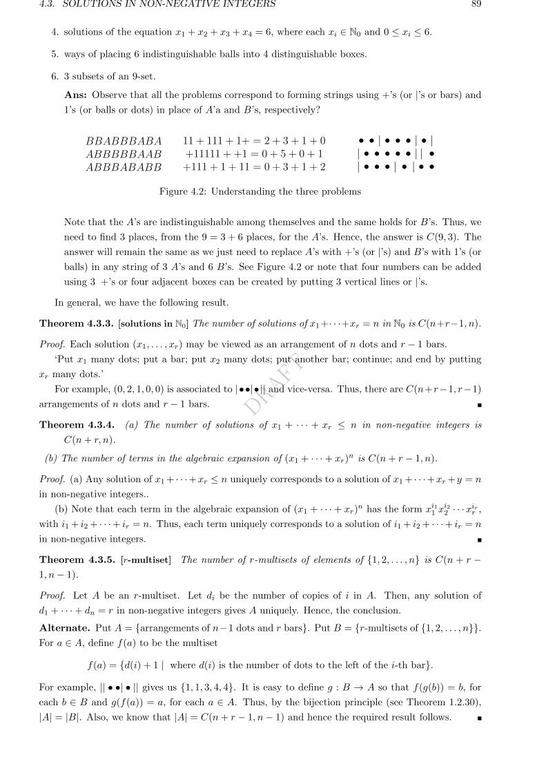
DRAFT

4.3. SOLUTIONS IN NON-NEGATIVE INTEGERS 89

4. solutions of the equation x1 + x2 + x3 + x4 = 6, where each xi ∈ N0 and 0 ≤ xi ≤ 6.

5. ways of placing 6 indistinguishable balls into 4 distinguishable boxes.

6. 3 subsets of an 9-set.

Ans: Observe that all the problems correspond to forming strings using +’s (or |’s or bars) and

1’s (or balls or dots) in place of A’a and B’s, respectively?

ABBBABABBABBBBBAABBBABBBABA

+111 + 1 + 11 = 0 + 3 + 1 + 2+11111 + +1 = 0 + 5 + 0 + 111 + 111 + 1+ = 2 + 3 + 1 + 0

| • • • | • | • •| • • • • • | | •• • | • • • | • |

1

Figure 4.2: Understanding the three problems

Note that the A’s are indistinguishable among themselves and the same holds for B’s. Thus, we

need to find 3 places, from the 9 = 3 + 6 places, for the A’s. Hence, the answer is C(9, 3). The

answer will remain the same as we just need to replace A’s with +’s (or |’s) and B’s with 1’s (or

balls) in any string of 3 A’s and 6 B’s. See Figure 4.2 or note that four numbers can be added

using 3 +’s or four adjacent boxes can be created by putting 3 vertical lines or |’s.

In general, we have the following result.

Theorem 4.3.3. [solutions in N0] The number of solutions of x1+· · ·+xr = n in N0 is C(n+r−1, n).

Proof. Each solution (x1, . . . , xr) may be viewed as an arrangement of n dots and r − 1 bars.

‘Put x1 many dots; put a bar; put x2 many dots; put another bar; continue; and end by putting

xr many dots.’

For example, (0, 2, 1, 0, 0) is associated to |••|• || and vice-versa. Thus, there are C(n+r−1, r−1)

arrangements of n dots and r − 1 bars.

Theorem 4.3.4. (a) The number of solutions of x1 + · · · + xr ≤ n in non-negative integers is

C(n+ r, n).

(b) The number of terms in the algebraic expansion of (x1 + · · ·+ xr)n is C(n+ r − 1, n).

Proof. (a) Any solution of x1 + · · ·+xr ≤ n uniquely corresponds to a solution of x1 + · · ·+xr +y = n

in non-negative integers..

(b) Note that each term in the algebraic expansion of (x1 + · · ·+ xr)n has the form xi11 x

i22 · · ·xirr ,

with i1 + i2 + · · ·+ ir = n. Thus, each term uniquely corresponds to a solution of i1 + i2 + · · ·+ ir = n

in non-negative integers.

Theorem 4.3.5. [r-multiset] The number of r-multisets of elements of 1, 2, . . . , n is C(n + r −1, n− 1).

Proof. Let A be an r-multiset. Let di be the number of copies of i in A. Then, any solution of

d1 + · · ·+ dn = r in non-negative integers gives A uniquely. Hence, the conclusion.

Alternate. Put A = arrangements of n−1 dots and r bars. Put B = r-multisets of 1, 2, . . . , n.For a ∈ A, define f(a) to be the multiset

f(a) = d(i) + 1 | where d(i) is the number of dots to the left of the i-th bar.

For example, || • •| • || gives us 1, 1, 3, 4, 4. It is easy to define g : B → A so that f(g(b)) = b, for

each b ∈ B and g(f(a)) = a, for each a ∈ A. Thus, by the bijection principle (see Theorem 1.2.30),

|A| = |B|. Also, we know that |A| = C(n+ r − 1, n− 1) and hence the required result follows.

DRAFT


Example 4.3.6. 1. There are 5 kinds of ice-creams available in our market complex. In how many

ways can you buy 15 of them for a party?

Ans: Suppose you buy xi ice-creams of the i-th type. Then, the problem is the same as finding

the number of solutions of x1 + · · ·+ x5 = 15 in non-negative integers.

2. How many solutions in N0 are there to x+ y + z = 60 such that x ≥ 3, y ≥ 4, z ≥ 5?

Ans: (x, y, z) is such a solution if and only if (x− 3, y− 4, z− 5) is a solution to x+ y+ z = 48

in N0. So, answer is C(50, 2).

3. How many solutions in N0 are there to x + y + z = 60 such that 20 ≥ x ≥ 3, 30 ≥ y ≥ 4, 40 ≥z ≥ 5?

Ans: We are looking for solution in N0 of x+ y + z = 48 such that x ≤ 17, y ≤ 26 and z ≤ 35.

Let A = (x, y, z) ∈ N30 | x + y + z = 48, Ax = (x, y, z) ∈ N3

0 | x + y + z = 48, x ≥ 18,Ay = (x, y, z) ∈ N3

0 | x+ y+ z = 48, y ≥ 27 and Az = (x, y, z) ∈ N30 | x+ y+ z = 48, z ≥ 36.

We know that |A| = C(50, 2). Our answer is then C(50, 2)− |Ax ∪Ay ∪Az|. Very soon we will

learn to find the value of |Ax ∪Ay ∪Az|.Exercise 4.3.7. 1. Determine the number of solutions of x+ y + z = 7 with x, y, z ∈ N?

2. Find the number of allocations of n identical objects to r distinct locations so that location i gets

at least pi ≥ 0 elements, i = 1, 2, · · · , r.

3. In how many ways can we pick integers x1 < x2 < x3 < x4 < x5, from 1, 2, . . . , 20 so that

xi − xi−1 ≥ 3, i = 2, 3, 4, 5? Solve in three different ways.

4. Find the number of solutions in non-negative integers of a+ b+ c+ d+ e < 11.

5. In a room, there are 2 distinct book racks with 5 shelves each. Each shelf is capable of holding

up to 10 books. In how many ways can we place 10 distinct books in two racks?

6. How many 4-letter words (with repetition) are there with the letters in alphabetical order?

7. Determine the number of non-decreasing sequences of length r using the numbers 1, 2, . . . , n.

8. In how many ways can m indistinguishable balls be put into n distinguishable boxes with the

restriction that no box is empty.

9. How many 26-letter permutations of the ENGLISH alphabets have no 2 vowels together?

10. How many 26-letter permutations of the ENGLISH alphabets have at least two consonants be-

tween any two vowels?

11. How many ways are there to select 10 integers from the set 1, 2, . . . , 100 such that the positive

difference between any two of the 10 integers is at least 3.

12. How many 10-element subsets of the ENGLISH alphabets do not have a pair of consecutive

letters?

13. How many 10-element subsets of the ENGLISH alphabets have a pair of consecutive letters?

14. How many ways are there to distribute 50 balls to 5 persons if Ram and Shyam together get no

more than 30 and Mohawk gets at least 10?

15. How many arrangements of the letters of KAGARTHALAMNAGARTHALAM have no 2 vowels

adjacent?

16. How many arrangements of the letters of RECURRENCERELATION have no 2 vowels adja-

cent?

DRAFT

4.4. SET PARTITIONS 91

17. How many ways are there to arrange the letters in ABRACADABARAARCADA such that the

first

(a) A precedes the first B?

(b) B precedes the first A and the first D precedes the first C?

(c) B precedes the first A and the first A precedes the first C?

18. How many ways are there to arrange the letters in KAGARTHALAMNAGARTHATAM such

that the first

(a) A precedes the first T?

(b) M precedes the first G and the first H precedes the first A?

(c) M precedes the first G and the first T precedes the first G?

19. In how many ways can we pick 20 letters from 10 A’s, 15 B’s and 15 C’s?

20. Determine the number of ways to sit 10 men and 7 women so that no 2 women sit next to each

other?

21. How many ways can 8 persons, including Ram and Shyam, sit in a row with Ram and Shyam

not sitting next to each other?

22. Evaluaten∑

i1=1

i1∑i2=1

i2∑i3=1· · ·

ik−1∑ik=1

1.

23. Evaluate9∑

i1=1

i1∑i2=1

i2∑i3=1· · ·

i8∑i9=1

i29.

4.4 Set Partitions

Recall that a partition of a set S is a collection of pairwise disjoint nonempty subsets whose union is

S. For clarity, let us look at a few examples once again.

Example 4.4.1. (a)1, 2, 3, 4, 5, 6

,1, 3, 2, 4, 5, 6

and

1, 2, 3, 4, 5, 6

are both

partitions of 1, 2, 3, 4, 5, 6 into 3 subsets.

(b) There are 2n−1 − 1 partitions of 1, 2, . . . , n, n ≥ 2 into two subsets. To see this, observe that

for each nontrivial subset A ∈ P(1, 2, . . . , n), the set A,Ac is a partition of 1, 2, . . . , n into

two subsets. Since, the total number of nontrivial subsets of P(1, 2, . . . , n) equals 2n − 2, the

required result follows.

(c) Number of allocations of 7 students into 7 different project groups so that each group has one

student, is 7! = C(7; 1, 1, 1, 1, 1, 1, 1) but the number of partitions of a set of 7 students into 7

subsets is 1.

(d) In how many ways can I write1, 2, 3, 4, 5, 6, 7, 8, 9, 10, 11, 12

on a piece of paper,

with the condition that sets have to be written in a row in increasing size?

DRAFT


Ans: Let us write a few first.1, 2, 3, 4, 5, 6, 7, 8, 9, 10, 11, 12

correct

2, 1, 3, 4, 5, 6, 7, 8, 9, 10, 11, 12

correct5, 6, 3, 4, 1, 2, 10, 11, 12, 9, 7, 8

correct

2, 3, 1, 4, 5, 6, 7, 8, 9, 10, 11, 12

incorrect, not the same partition2, 1, 3, 4, 7, 8, 9, 5, 6, 10, 11, 12

incorrect, not satisfying the condition

There are 3!(2!)3×2!(3!)2 ways. Notice that from each written partition, if I remove the brackets

I get an arrangement of elements of 1, 2, . . . , 12.

(e) How many arrangements do I generate from a partition with pi subsets of size ni, n1 < · · · < nk?

Ans: p1!(n1!)p1 · · · pk!(nk!)pk =

k∏i=1

[pi!(ni!)pi ].

Theorem 4.4.2. [Set partition] The number of partitions of 1, 2, . . . , n with pi subsets of size ni,

n1 < · · · < nk isn!

(n1!)p1p1! · · · (nk!)pkpk!.

Proof. Note that each such partition generatesk∏i=1

[pi!(ni!)pi ] arrangement of elements of 1, 2, . . . , n.

Conversely, for each arrangement of elements of 1, 2, . . . , n we can easily construct a partition of the

above type which can generate this arrangement. Thus, the proof is complete.

Definition 4.4.3. Stirling numbers of the second kind, denoted S(n, r), is the number of par-

titions of 1, 2, . . . , n into r-subsets (r-parts). By convention, S(n, r) = 1, if n = r and 0, whenever

either ‘n > 0 and r = 0’ or ‘n < r’.

Theorem 4.4.4. [recurrence for S(n, r)] S(n+ 1, r) = S(n, r − 1) + rS(n, r).

Proof. Write an r-partition of 1, 2, . . . , n, n + 1 and erase n + 1 from it. That is, if n + 1 is an

element of an r-partition, then the number of such partitions become S(n, r − 1); else n + 1 appears

in one of the element of an r-partition of 1, 2, . . . , n, which gives the number rS(n, r).

Example 4.4.5. Determine the number of ways of putting n distinguishable/distinct balls into r

indistinguishable boxes with the restriction that no box is empty.

Ans: Let A be the set of n distinct balls and let the balls in i-th box be Bi, 1 ≤ i ≤ r.

1. Since each box is non-empty, each Bi is non-empty.

2. Also, each ball is in some box and hencer⋃i=1

Bi = A.

3. As the boxes are indistinguishable, we arrange the boxes in non-increasing order, i.e., |B1| ≥· · · ≥ |Br|.

Thus, B1, B2, . . . , Br is a partition of A into r-parts. Hence, the required number of ways is given by

S(n, r), the Stirling number of the second kind.

To proceed further, consider the following example.

DRAFT

4.4. SET PARTITIONS 93

Example 4.4.6. Let A = a, b, c, d, e and S = 1, 2, 3. Define an onto function f : A → S by

f(a) = f(b) = f(c) = 1, f(d) = 2 and f(e) = 3. Then, f gives a partition B1 = a, b, c, B2 = d and

B3 = e of A into 3-parts. Also, let A1 = a, d, A2 = b, e and A3 = c be a partition of A into

3-parts. Then, this partition gives 3! onto functions from A into S, each of them being a one-to-one

function from A1, A2, A3 to S, namely,

f1(a) = f1(d) = 1, f1(b) = f1(e) = 2, f1(c) = 3, ⇔ f1(A1) = 1, f1(A2) = 2, f1(A3) = 3





f6(a) = f6(d) = 3, f6(b) = f6(e) = 2, f6(c) = 1, ⇔ f6(A1) = 3, f6(A2) = 2, f6(A3) = 1.

Lemma 4.4.7. The total number of onto functions f : 1, 2, . . . , r → 1, 2, . . . , n is n!S(r, n).

Proof. ‘f is onto’ means ‘for all y ∈ 1, 2, . . . , n there exists x ∈ 1, 2, . . . , r, such that f(x) = y’.

Therefore, the number of onto functions is 0, whenever r < n. So, we assume that r ≥ n. Then,

1. for each i ∈ 1, 2, . . . , n, f−1(i) = x ∈ 1, 2, . . . , r | f(x) = i is a non-empty set (f is onto).

2. f−1(i) ∩ f−1(j) = ∅, whenever 1 ≤ i 6= j ≤ n (f is a function).

3.n⋃i=1

f−1(i) = 1, 2, . . . , r (domain of f is 1, 2, . . . , r).

Therefore, f−1(i)’s give a partition of 1, 2, . . . , r into n-parts. Also, note that each such function f ,

gives a one-to-one function from f−1(1), . . . , f−1(r) to 1, 2, . . . , n.Conversely, for each partition A1, A2, . . . , An of 1, 2, . . . , r into n-parts, we get n! one-to-one

function from A1, A2, . . . , An to 1, 2, . . . , n. Hence,∣∣f : 1, 2, . . . , r → 1, 2, . . . , n | f is onto∣∣ =∣∣g : A1, A2, . . . , An → 1, 2, . . . , n | g is one-to-one

∣∣×∣∣Partition of 1, 2, . . . , r into n-parts∣∣ = n! S(r, n).


Lemma 4.4.8. Let r, n ∈ N and ` = minr, n. Then,

nr =∑k=1

C(n, k)k!S(r, k). (4.1)

Proof. Let A = f | f : 1, 2, . . . , r → 1, 2, . . . , n. We compute |A| by two different methods.

Method 1: By Theorem 4.1.2, |A| = nr.

Method 2: Let f0 : 1, 2, . . . , r → 1, 2, . . . , n be any function. Then, f0 is an onto function from

1, 2, . . . , r to Im (f0) = f0(1, 2, . . . , r). Moreover, , for some k, 1 ≤ k ≤ ` = minr, n. Thus,

A =⋃k=1

Ak, where Ak = f : 1, 2, . . . , r → 1, 2, . . . , n | |f(1, 2, . . . , r)| = k and Ak ∩ Aj = ∅,whenever 1 ≤ j 6= k ≤ `. Now, using Theorem 4.1.18, a subset of 1, 2, . . . , n of size k can be selected

in C(n, k) ways. Thus, for 1 ≤ k ≤ `,

|Ak| =∣∣K : K ⊆ 1, 2, . . . , n, |K| = k

∣∣× ∣∣f : 1, 2, . . . , r → K | f is onto∣∣ = C(n, k)k!S(r, k).

DRAFT


Therefore,

|A| =∣∣∣∣∣ ⋃k=1

Ai

∣∣∣∣∣ =∑k=1

|Ak| =∑k=1

C(n, k)k!S(r, k).

Hence, using the two counting methods, the required result follows.

Remark 4.4.9. 1. The following two problems are equivalent.

(a) Count the number of onto functions f : 1, 2, . . . , r → 1, 2, . . . , n.(b) Count the number ways to put r distinguishable/distinct balls into n distinguishable/distinct

boxes so that no box is empty.

2. The numbers S(r, k) can be recursively calculated using Equation (4.1). For example, we show

that S(m, 1) = 1, for all m ≥ 1.

Ans: Take n ≥ 1 and r = 1 in Equation (4.1) to get

n = n1 =

1∑k=1

C(n, k)k!S(1, k) = C(n, 1)1!S(1, 1) = nS(1, 1).

Thus, S(1, 1) = 1. Take n = 1 and r ≥ 2 in Equation (4.1) to get

1 = 1r =1∑

k=1

C(1, k)k!S(r, k) = S(r, 1).

3. As exercise, verify that S(5, 2) = 15, S(5, 3) = 25, ;S(5, 4) = 10, S(5, 5) = 1.

Exercise 4.4.10. 1. Determine the number of ways of

(a) selecting r distinguishable objects from n distinguishable objects, when n ≥ r.

(b) distributing 20 distinct toys among 4 children if each children gets 5 toys?

(c) placing r distinguishable balls into n indistinguishable boxes if no box is empty?

(d) placing r distinguishable balls into n indistinguishable boxes?

2. For n ∈ N, let b(n) denote the number of partitions of the set 1, 2, . . . , n. Then, b(n) =n∑r=0

S(n, r) is called the nth Bell number. By definition, b(0) = 1 = b(1). Determine b(n), for

2 ≤ n ≤ 5.

3. Fix n ∈ N. Then, a composition of n is an expression of n as a sum of positive integers. For

example, if n = 4, then the distinct compositions are

4, 3 + 1, 1 + 3, 2 + 2, 2 + 1 + 1, 1 + 1 + 2, 1 + 2 + 1, 1 + 1 + 1 + 1.

Let Sk(n) denote the number of compositions of n into k parts. Then, S1(4) = 1, S2(4) =

3, S3(4) = 3 and S4(4) = 1. Determine Sk(n), for 1 ≤ k ≤ n and∑k≥1

Sk(n).

4. Let S = f | f : 1, 2, . . . , r → 1, 2, . . . , n. Compute |S| in two ways to prove (n + 1)r =r∑

k=0

C(r, k)nk.

5. Suppose 13 people get on the lift at level . If all the people get down at some level, say 1, 2, 3, 4

and 5 then, calculate the number of ways of getting down if at least one person gets down at each

level.

DRAFT

4.5. LATTICE PATHS AND CATALAN NUMBERS 95

Definition 4.4.11. [Partition of a number] Let n, k ∈ N. A partition of n into k parts is a tuple

(x1, · · · , xk) ∈ Nk written in non-increasing order such that x1 + · · ·+ xk = n. It may be viewed as a

k-multiset S ⊆ N with sum n. By πn(k), we denote the number of partitions of n into exactly k parts

and by πn, the number of partitions of n. Conventionally π0 = 1 and πn(k) = 0, whenever k > n.

Remark 4.4.12. π7(4) = 3 as the partitions of 7 into 4-parts are 4 + 1 + 1 + 1, 3 + 2 + 1 + 1 and

2 + 2 + 2 + 1. Verify that π7(2) = 3 and π7(3) = 4.

Example 4.4.13. Determine the number of ways of placing r indistinguishable balls into n indistin-

guishable boxes

1. with the restriction that no box is empty.

Ans: As the balls are indistinguishable, we need to count the number of balls in each box. As

the boxes are indistinguishable, arrange them so that the number of balls inside boxes are in

non-increasing order. Also, each box is non-empty and hence the answer is πr(n).

2. with no restriction.

Ans: Let us place one ball in each box. Now ‘placing r indistinguishable ball into n indis-

tinguishable boxes with no restriction’ is same as ‘placing r + n indistinguishable balls into n

indistinguishable boxes so that no box is empty.’ Therefore, the required answer is πm+n(n).

Exercise 4.4.14. 1. Calculate π(n), for n = 1, 2, 3, . . . , 8.

2. Prove that π2r(r) = π(r), for any r ∈ N.

3. For a fixed n ∈ N determine a recurrence relation for the numbers πn(r)’s for 1 ≤ r ≤ n.

Definition 4.4.15. The Stirling number of the first kind, denoted s(n, k), is the coefficient of xk

in xn, where xn is called the falling factorial and equals x(x− 1)(x− 2) · · · (x− n+ 1). The rising

factorial xn is defined as x(x+ 1)(x+ 2) · · · (x+ n− 1).

Exercise 4.4.16. Prove by induction that

1. s(n,m)(−1)n−m is the coefficient of xm in xn and |s(n,m)| = s(n,m)(−1)n−m.

2. Let a(n, k) denote the number of permutations of 1, 2, . . . , n which have k disjoint cycles.

For example, a(4, 2) = 11 as it corresponds to the permutations (12)(34), (13)(24), (14)(23),

(1)(234), (1)(243), (134)(2), (143)(2), (124)(3), (142)(3), (123)(4) and (132)(4). By convention,

a(0, 0) = 1 and a(n, 0) = 0 = a(0, n), whenever n ≥ 1. Determine prove that the numbers

a(n, k)’s satisfy

a(n, k) = (n− 1)a(n− 1, k) + a(n− 1, k − 1).

3. Prove that a(n,m) = |s(n,m)| for all n,m ∈ N0.

4.5 Lattice Paths and Catalan Numbers

Consider a lattice of integer lines in R2 and let S = (m,n) | m,n = 0, 1, . . . be the said of points on

the lattice. For a pair of points, say A = (m1, n1) and B = (m2, n2) with m1 ≤ m2 and n1 ≤ n2, we

define a lattice path from A to B to be a subset e1, . . . , ek of S such that if ei = (x, y) then ei+1

is either (x+ 1, y) or (x, y+ 1), for 1 ≤ i ≤ k− 1. That is, at each step we move either one unit right,

denoted R, or one unit up, denoted U (see Figure 4.3).

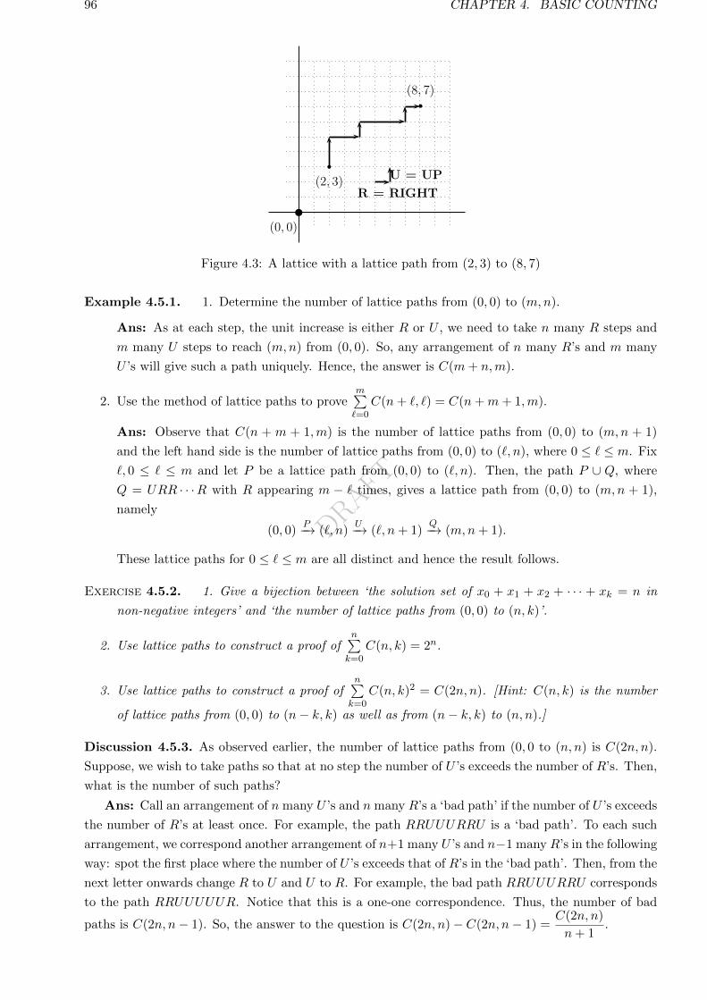
DRAFT


(0, 0)

(2, 3)

(8, 7)

R = RIGHT

U = UP

1

Figure 4.3: A lattice with a lattice path from (2, 3) to (8, 7)

Example 4.5.1. 1. Determine the number of lattice paths from (0, 0) to (m,n).

Ans: As at each step, the unit increase is either R or U , we need to take n many R steps and

m many U steps to reach (m,n) from (0, 0). So, any arrangement of n many R’s and m many

U ’s will give such a path uniquely. Hence, the answer is C(m+ n,m).

2. Use the method of lattice paths to provem∑=0

C(n+ `, `) = C(n+m+ 1,m).

Ans: Observe that C(n + m + 1,m) is the number of lattice paths from (0, 0) to (m,n + 1)

and the left hand side is the number of lattice paths from (0, 0) to (`, n), where 0 ≤ ` ≤ m. Fix

`, 0 ≤ ` ≤ m and let P be a lattice path from (0, 0) to (`, n). Then, the path P ∪ Q, where

Q = URR · · ·R with R appearing m − ` times, gives a lattice path from (0, 0) to (m,n + 1),

namely

(0, 0)P−→ (`, n)

U−→ (`, n+ 1)Q−→ (m,n+ 1).

These lattice paths for 0 ≤ ` ≤ m are all distinct and hence the result follows.

Exercise 4.5.2. 1. Give a bijection between ‘the solution set of x0 + x1 + x2 + · · · + xk = n in

non-negative integers’ and ‘the number of lattice paths from (0, 0) to (n, k)’.

2. Use lattice paths to construct a proof ofn∑k=0

C(n, k) = 2n.

3. Use lattice paths to construct a proof ofn∑k=0

C(n, k)2 = C(2n, n). [Hint: C(n, k) is the number

of lattice paths from (0, 0) to (n− k, k) as well as from (n− k, k) to (n, n).]

Discussion 4.5.3. As observed earlier, the number of lattice paths from (0, 0 to (n, n) is C(2n, n).

Suppose, we wish to take paths so that at no step the number of U ’s exceeds the number of R’s. Then,

what is the number of such paths?

Ans: Call an arrangement of n many U ’s and n many R’s a ‘bad path’ if the number of U ’s exceeds

the number of R’s at least once. For example, the path RRUUURRU is a ‘bad path’. To each such

arrangement, we correspond another arrangement of n+1 many U ’s and n−1 many R’s in the following

way: spot the first place where the number of U ’s exceeds that of R’s in the ‘bad path’. Then, from the

next letter onwards change R to U and U to R. For example, the bad path RRUUURRU corresponds

to the path RRUUUUUR. Notice that this is a one-one correspondence. Thus, the number of bad

paths is C(2n, n− 1). So, the answer to the question is C(2n, n)− C(2n, n− 1) =C(2n, n)

n+ 1.

DRAFT

4.5. LATTICE PATHS AND CATALAN NUMBERS 97

Definition 4.5.4. [Catalan number] The nth Catalan number, denoted Cn, is the number of

different representations of the product A1 · · ·An+1 of n+ 1 square matrices of the same size using n

pairs of brackets. By convention C0 = 1.

Theorem 4.5.5. [Catalan number] Prove that Cn = C(2n,n)n+1 for all n ∈ N.

Proof. Claim: After the (n−k)-th ‘(’, there are at least k+2 many A’s. To see this pick the substring

starting right from the (n−k)-th ‘(’ till we face (k+ 1) many ‘)’s. This substring represents a product

of matrices. So, it must contain (k + 2) many Ai’s.

Given one representation of the product, replace each Ai by A. Drop the right brackets to have a

sequence of n many ‘(’s and n + 1 many A’s. Thus, the number of A’s used till the n − kth ‘(’ is at

most n+ 1− (k + 2) = n− k − 1. So, the number of A’s never exceeds the number of ‘(’.

Conversely, given such an arrangement, we can put back the ‘)’s: find two consecutive letters from the

last ‘(’; put a right bracket after them; treat (AA) as a letter; repeat the process. For example,

((A((AAAA→ ((A((AA)AA→ ((A((AA)A)A→ ((A((AA)A))A = ((A((AA)A))A)

By previous example the number of such arrangements is C(2n,n)n+1 .

The readers who are interested in knowing more about Catalan numbers should look at the book

“enumerative combinatorics” by Stanley [12].

Exercise 4.5.6. 1. Give a recurrence relation for Cn’s (i.e., a formula for Cn involving C0, . . . , Cn−1).

Hence, show that Cn = C(2n, n)/(n+ 1).

2. Give an arithmetic proof of the fact that (n+ 1) divides C(2n, n).

3. A man is standing on the edge of a swimming pool (facing it) holding a bag containing n blue

and n red balls. He randomly picks up one ball at a time and discards it. If the ball is blue he

takes a step back and if the ball is red, he takes a step forward. What is the probability of his

falling into the swimming pool?

4. Consider a regular polygon with vertices 1, 2, · · · , n. In how many ways can we divide the polygon

into triangles using (n− 3) non-crossing diagonals?

5. How many arrangements of n blue and n red balls are there such that at any position in the

arrangement the number of blue balls (till that position) is at most one more than the number of

red balls (till that position)?

6. We want to write a matrix of size 10 × 2 using numbers 1, . . . , 20 with each number appearing

exactly once. Then, determine the number of such matrices in which the numbers

(a) increase from left to right?

(b) increase from up to down?

(c) increase from left to right and up to down?

7. How many lattice paths are there from (0, 0) to (9, 9) which does not cross the dotted line?

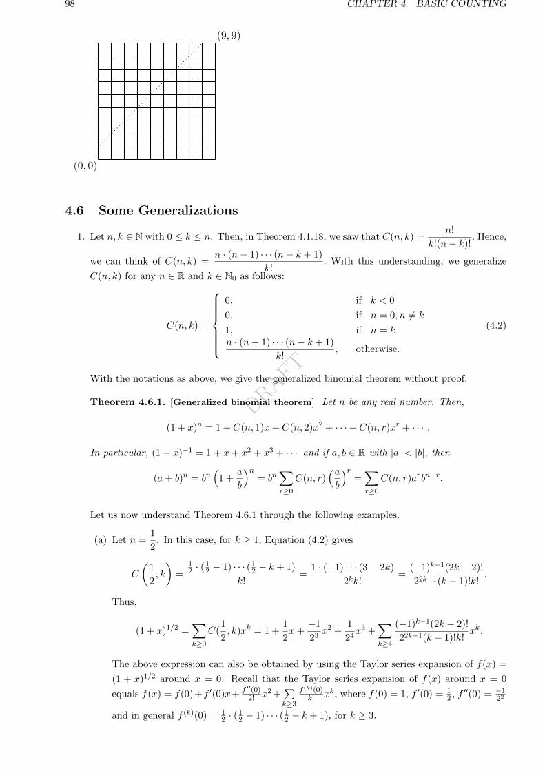
DRAFT


(0, 0)

(9, 9)

1

4.6 Some Generalizations

1. Let n, k ∈ N with 0 ≤ k ≤ n. Then, in Theorem 4.1.18, we saw that C(n, k) =n!

k!(n− k)!. Hence,

we can think of C(n, k) =n · (n− 1) · · · (n− k + 1)

k!. With this understanding, we generalize

C(n, k) for any n ∈ R and k ∈ N0 as follows:

C(n, k) =

0, if k < 0

0, if n = 0, n 6= k

1, if n = kn · (n− 1) · · · (n− k + 1)

k!, otherwise.

(4.2)

With the notations as above, we give the generalized binomial theorem without proof.

Theorem 4.6.1. [Generalized binomial theorem] Let n be any real number. Then,

(1 + x)n = 1 + C(n, 1)x+ C(n, 2)x2 + · · ·+ C(n, r)xr + · · · .

In particular, (1− x)−1 = 1 + x+ x2 + x3 + · · · and if a, b ∈ R with |a| < |b|, then

(a+ b)n = bn(

1 +a

b

)n= bn

∑r≥0

C(n, r)(ab

)r=∑r≥0

C(n, r)arbn−r.

Let us now understand Theorem 4.6.1 through the following examples.

(a) Let n =1

2. In this case, for k ≥ 1, Equation (4.2) gives

C

(1

2, k

)=

12 · (12 − 1) · · · (12 − k + 1)

k!=

1 · (−1) · · · (3− 2k)

2kk!=

(−1)k−1(2k − 2)!

22k−1(k − 1)!k!.

Thus,

(1 + x)1/2 =∑k≥0

C(1

2, k)xk = 1 +

1

2x+−1

23x2 +

1

24x3 +

∑k≥4

(−1)k−1(2k − 2)!

22k−1(k − 1)!k!xk.

The above expression can also be obtained by using the Taylor series expansion of f(x) =

(1 + x)1/2 around x = 0. Recall that the Taylor series expansion of f(x) around x = 0

equals f(x) = f(0)+f ′(0)x+ f ′′(0)2! x2 +

∑k≥3

f (k)(0)k! xk, where f(0) = 1, f ′(0) = 1

2 , f ′′(0) = −122

and in general f (k)(0) = 12 · (12 − 1) · · · (12 − k + 1), for k ≥ 3.

DRAFT

4.6. SOME GENERALIZATIONS 99

(b) Let n = −r, where r ∈ N. Then, for k ≥ 1, Equation (4.2) gives C(−r, k) =−r · (−r − 1) · · · (−r − k + 1)

k!=

(−1)kC(r + k − 1, k). Thus,

(1 + x)n =1

(1 + x)r= 1− rx+ C(r + 1, 2)x2 +

∑k≥3

C(r + k − 1, k)(−x)k.

2. Let n,m ∈ N. Recall the identity nm =m∑k=0

C(n, k)k!S(m, k) =n∑k=0

C(n, k)k!S(m, k) in Equa-

tion (4.1). Note that for each m ∈ N, the above identity equals X = AY , where

X =

0m

1m

2m

3m

...

nm

, A =

C(0, 0) 0 0 · · · 0

C(1, 0) C(1, 1) 0 · · · 0

C(2, 0) C(2, 1) C(2, 2) · · · 0...

......

. . ....

C(n, 0) C(n, 1) C(n, 2) · · · C(n, n)

and Y =

0!S(m, 0)

1!S(m, 1)

2!S(m, 2)...

n!S(m,n)

.

As A is lower triangular with det(A) = 1, it has an inverse and each entry of A−1 has a similar

form. So, Y = A−1X, where

A−1 =

C(0, 0) 0 0 0 · · · 0

−C(1, 0) C(1, 1) 0 0 · · · 0

C(2, 0) −C(2, 1) C(2, 2) 0 · · · 0

−C(3, 0) C(3, 1) −C(3, 2) C(3, 3) · · · 0...

......

.... . .

...

(−1)nC(n, 0) (−1)n−1C(n, 1) (−1)n−2C(n, 2) (−1)n−3C(n, 3) · · · C(n, n)

.

Hence, for n,m ∈ N, we have

S(m,n) =1

n!

∑k≥0

(−1)kC(n, k)(n− k)m. (4.3)

3. The above matrix inversion implies that for n ∈ N0, the identity

a(n) =∑k≥0

C(n, k)b(k) holds if and only if b(n) =∑k≥0

(−1)kC(n, k)a(k) holds.

We end this chapter with another set of exercises.

Exercise 4.6.2. 1. Prove that there exists a bijection between any two of the following sets.

(a) The set of words of length n on an alphabet consisting of m letters.

(b) The set of maps of an n-set into an m-set.

(c) The set of distributions of n distinct objects into m distinct boxes.

(d) The set of n-tuples on m letters.

2. Prove that there exists a bijection between any two of the following sets.

(a) The set of n letter words with distinct letters out of an alphabet consisting of m letters.

(b) The set of one-one functions from an n-set into an m-set.

(c) The set of distributions of n distinct objects into m distinct boxes, subject to ‘if an object

is put in a box, no other object can be put in the same box’.

DRAFT


(d) The set of n-tuples on m letters, without repetition.

(e) The set of permutations of m symbols taken n at a time.

3. Prove that there exists a bijection between any two of the following sets.

(a) The set of increasing words of length n on m ordered letters.

(b) The set of distributions on n non-distinct objects into m distinct boxes.

(c) The set of combinations of m symbols taken n at a time with repetitions permitted.

DRAFT

Chapter 5

Advanced Counting Principles

5.1 Pigeonhole Principle

Discussion 5.1.1. [Pigeonhole principle (PHP)]

PHP1. If n+ 1 pigeons stay in n holes then there is a hole with at least two pigeons.

PHP2. If kn+ 1 pigeons stay in n holes then there is a hole with at least k + 1 pigeons.

PHP3. If p1 + · · ·+ pn + 1 pigeons stay in n holes then there is a hole i with at least pi + 1 pigeons.

Example 5.1.2. 1. Consider a tournament of n > 1 players, where each pair plays exactly once

and each player wins at least once. Then, there are two players with the same number of wins.

Ans: Number of wins vary from 1 to n− 1 and there are n players.

2. A bag contains 5 red, 8 blue, 12 green and 7 yellow marbles. The least number of marbles to be

chosen to ensure that there are

(a) at least 4 marbles of the same color is 13,

(b) at least 7 marbles of the same color is 24,

(c) at least 4 red or at least 7 of any other color is 22.

3. In a group of 6 people, prove that there are three mutual friends or three mutual strangers.

Ans: Let a be a person in the group. Let F be the set of friends of a and S the set of strangers

to a. Clearly |S|+ |F | = 5. By PHP either |F | ≥ 3 or |S| ≥ 3.

Case 1: |F | ≥ 3. If any two in F are friends then those two along with a are three mutual

friends. Else F is a set of mutual strangers of size at least 3.

Case 2: |S| ≥ 3. If any pair in S are strangers then those two along with a are three mutual

strangers. Else S becomes a set of mutual friends of size at least 3.

4. If 7 points are chosen inside or on the unit circle, then there is a pair of points which are at a

distance at most 1.

Ans: To see this divide the circle into 6 equal cone type parts creating an angle of 60o with the

center. By PHP there is a part containing at least two points. The distance between these two

is at most 1.

5. If n+1 integers are selected from 1, 2, . . . , 2n, then there is a pair which has the property that

one of them divides the other.

Ans: Each number has the form 2ks, where s = 2m + 1 is an odd number. There are n odd

numbers. If we select n+1 numbers from S, by PHP some two of them (say, x, y) have the same

odd part, that is, x = 2is and y = 2js. If i ≤ j, then x|y, otherwise y|x.

101

DRAFT

102 CHAPTER 5. ADVANCED COUNTING PRINCIPLES

6. (a) Let r1, r2, · · · , rmn+1 be a sequence of mn+1 distinct real numbers. Then, prove that there

is a subsequence of m + 1 numbers which is increasing or there is a subsequence of n + 1

numbers which is decreasing.

Ans: Define li to be the maximum length of an increasing subsequence starting at ri. If

some li ≥ m+ 1 then we have nothing to prove. So, let 1 ≤ li ≤ m. Since (li) is a sequence

of mn + 1 integers, by PHP, there is one number which repeats at least n + 1 times. Let

li1 = li2 = · · · = lin+1 = s, where i1 < i2 < · · · < in+1. Notice that ri1 > ri2 , because if

ri1 < ri2 , then ‘ri1 together with the increasing sequence of length s starting with ri2 ’ gives

an increasing sequence of length s + 1. Similarly, ri2 > ri3 > · · · > rin+1 and hence the

required result holds.

Alternate. Let S = r1, r2, · · · , rmn+1 and define a map f : S → Z×Z by f(ri) = (s, t),

for 1 ≤ i ≤ mn+1, where s equals the length of the largest increasing subsequence starting

with ri and t equals the length of the largest decreasing subsequence ending at ri. Now, if

either s ≥ m+ 1 or t ≥ n+ 1, we are done. If not, then note that 1 ≤ s ≤ m and 1 ≤ t ≤ n.

So, the number of tuples (s, t) is at most mn. Thus, the mn + 1 distinct numbers are

being mapped to mn tuples and hence by PHP there are two numbers ri 6= rj such that

f(ri) = f(rj). Now, proceed as in the previous case to get the required result.

(b) Does the above statement hold for every collection of mn distinct numbers? No. Consider

the sequence:

n, n−1, · · · , 1, 2n, 2n−1, . . . , n+1, 3n, 3n−1, · · · , 2n+1, · · · ,mn,mn−1, · · · ,mn−n+1.

7. Given any 1010 integers, prove that there is a pair that either differ by, or sum to, a multiple of

2017. Is this true if we replace 1010 by 1009?

Ans: Let the numbers be n1, n2, . . . , n1010 and S = n1 − nk, n1 + nk : k = 2, . . . , 1010. Then,

|S| = 2018 and hence, at least two of them will have the same remainder when divided by 2017.

Then, consider their difference. For the later part, consider 0, 1, 2, . . . , 1008.

8. Let a ∈ R \Q. Then, there are infinitely many rational numbers pq such that |a− p

q | < 1q2

.

Ans: Enough to show that there are infinitely many (p, q) ∈ Z2 with |qa − p| < 1q . As a is

irrational, note that for every m ∈ N, 0 < ia − biac < 1, for i = 1, . . . ,m + 1. Hence, by PHP

there exist i, j with i < j such that

|(j − i)a− (bjac − biac)| < 1

m≤ 1

j − i .

Then, the tuple (p1, q1) = (bjac−biac, j− i) satisfies the required property. To generate another

tuple, find m2 such that1

m2< |a− p1

q1|

and proceed as before to get (p2, q2) such that |q2a−p2| < 1m2≤ 1

q2. Since |a− p2

q2| < 1

m2< |a− p1

q1|,

we have p1q16= p2

q2. Now use induction to get the required result.

9. Prove that there exist two powers of 3 whose difference is divisible by 2017.

Ans: Let S = 1 = 30, 3, 32, 33, . . . , 32017. Then, |S| = 2018. As the remainders of any integer

when divided by 2017 is 0, 1, 2, . . . , 2016, by PHP, there is a pair which has the same remainder.

Hence, 2017 divides 3j − 3i for some i, j.

DRAFT

5.1. PIGEONHOLE PRINCIPLE 103

10. Prove that there exists a power of three that ends with 0001.

Ans: Let S = 1 = 30, 3, 32, 33, . . .. Now, divide each element of S by 104. As |S| > 104, by

PHP, there exist i > j such that the remainders of 3i and 3j , when divided by 104, are equal.

But gcd(104, 3) = 1 and thus, 104 divides 3` − 1. That is, 3` − 1 = s · 104 for some positive

integer s. That is, 3` = s · 104 + 1 and hence the result follows.

Exercise 5.1.3. 1. Consider the poset (X = P(1, 2, 3, 4),⊆). Write 6 maximal chains P1, . . . P6

(need not be disjoint) such that ∪iPi = X. Let A1, . . . , A7 be 7 distinct subsets of 1, 2, 3, 4.

Use PHP, to prove that there exist i, j such that Ai, Aj ∈ Pk, for some k. That is, A1, . . . , A7cannot be an anti-chain. Conclude that this holds as the width of the poset is 6.

2. Let x1, . . . , x9 ⊆ N with9∑i=1

xi = 30. Then, prove that there exist i, j, k ∈ 1, 2, . . . , 9 with

xi + xj + xk ≥ 12.

3. Pick any 6 integers from 1, 2, . . . , 10, then there exists a pair with odd sum.

4. Any 14-subset of 1, 2, . . . , 46 has four elements a, b, c, d such that a+ b = c+ d.

5. In a row of 12 chairs 9 are filled. Then, some 3 consecutive chairs are filled. Will 8 work?

6. Every n-sequence of integers has a consecutive subsequence with sum divisible by n.

7. Let n > 3 and S ⊆ 1, 2, . . . , n of size m = bn+22 c + 1. Then, there exist a, b, c ∈ S such that

a+ b = c.

8. Let a, b ∈ N, a < b. Given more than half of the integers in the set 1, 2, . . . , a + b, there is a

pair which differ by either a or b.

9. Consider a chess board with two of the diagonally opposite corners removed. Is it possible to

cover the board with pieces of rectangular dominos whose size is exactly two board squares?

10. Mark the centers of all squares of an 8 × 8 chess board. Is it possible to cut the board with 13

straight lines not passing through any center, so that every piece had at most 1 center?

11. Fifteen squirrels have 100 nuts. Then, some two squirrels have equal number of nuts.

12. Suppose that f(x) is a polynomial with integer coefficients. If

(a) f(x) = 2 for three distinct integers, then for no integer x, f(x) can be equal to 3.

(b) f(x) = 14 for three distinct integers, then for no integer x, f(x) can be equal to 15.

(c) f(x) = 11 for five distinct integers, then for no integer x, f(x) can be equal to 9.

13. Choose 5 points at random inside an equilateral triangle of side 1 unit, then there exists a pair

which have distance at most 0.5 units.

14. Prove that among any 55 integers 1 ≤ x1 < x2 < x3 < · · · < x55 ≤ 100, there is a pair with

difference 9, a pair with difference 10, a pair with difference 12 and a pair with difference 13.

Surprisingly, there need not be a pair with difference 11.

15. Let x1, x2, . . . , xn ⊆ Z. Prove that there exist 1 ≤ i ≤ j ≤ n such that

(a) xi + xi+1 + · · ·+ xj−1 + xj is a multiple of 2017, whenever n ≥ 2017.

(b) xj + xi or xj − xi is a multiple of 2017, whenever n ≥ 1010.

16. Let A and B be two discs, each having 2n equal sectors. On disc A, n sectors are colored red and

n are colored blue. The sectors of disc B are colored arbitrarily with red and blue colors. Show

that there is a way of putting the two discs, one above the other, so that at least n corresponding

sectors have the same colors.

DRAFT


17. There are 7 distinct real numbers. Is it possible to select two of them, say x and y such that

0 < x−y1+xy <

1√3?

18. If n is odd then for any permutation p of 1, 2, . . . , n the productn∏i=1

(i− p(i)

)is even.

19. Fix a positive α ∈ R \Q. Then, S = m+ nα : m,n ∈ Z is dense in R.

20. If more than half of the subsets of 1, 2, . . . , n are selected, then some two of the selected subsets

have the property that one is a subset of the other.

21. Given any ten 4-subsets of 1, 2, . . . , 11,, some two of them have at least 2 elements in common.

22. A person takes at least one aspirin a day for 30 days. If he takes 45 aspirin altogether then prove

that in some sequence of consecutive days he takes exactly 14 aspirins.

23. If 58 entries of a 14× 14 matrix are 1, then there is a 2× 2 submatrix with all entries 1.

24. Let A and B be two finite non-empty sets with B = b1, b2, . . . , bm. Let f : A → B be any

function. Then, for any non-negative integers a1, a2, . . . , am if |A| = a1 + a2 + · · ·+ am −m+ 1

then prove that there exists an i, 1 ≤ i ≤ m such that |f−1(bi)| ≥ ai.25. Each of the given 9 lines cuts a given square into two quadrilaterals whose areas are in the ratio

2 : 3. Prove that at least three of these lines pass through the same point.

26. Five points are chosen at the nodes of a square lattice (view Z × Z). Why is it certain that a

mid-point of some two of them is a lattice point?

27. Take 25 points on a plane satisfying ‘among any three of them there is a pair at a distance less

than 1’. Then, some circle of unit radius contains at least 13 of the given points.

28. If each point of a circle is colored either red or blue, then show that there exists an isosceles

triangle with vertices of the same color.

29. Each point of the plane is colored red or blue, then prove the following.

(a) There exist two points of the same color which are at a distance of 1 unit.

(b) There is an equilateral triangle all of whose vertices have the same color.

(c) There is a rectangle all of whose vertices have the same color.

30. Let S ⊆ 1, 2, . . . , 100 be a 10-set. Then, some two disjoint subsets of S have equal sum.

31. Fix a positive integer n. Prove that there exists an ` ∈ N such that n divides 2` − 1.

32. Does there exist a multiple of 2017 that is formed using only the digits

(a) 2? Justify your answer.

(b) 2 and 3 and the number of 2’s and 3’s are equal? Justify your answer.

33. Each natural number has a multiple of the form 9 · · · 90 · · · 0, with at least one 9.

5.2 Principle of Inclusion and Exclusion

We start this section with the following example.

Example 5.2.1. How many natural numbers n ≤ 1000 are not divisible by any of 2, 3?

Ans: Let A2 = n ∈ N | n ≤ 1000, 2|n and A3 = n ∈ N | n ≤ 1000, 3|n. Then, |A2 ∪ A3| =

|A2|+ |A3| − |A2 ∩A3| = 500 + 333− 166 = 667. So, the required answer is 1000− 667 = 333.

We now generalize the above idea whenever we have 3 or more sets.

DRAFT

5.2. PRINCIPLE OF INCLUSION AND EXCLUSION 105

Theorem 5.2.2. [Principle of inclusion and exclusion] Let A1, · · · , An be finite subsets of a set U .

Then, ∣∣ n∪i=1

Ai∣∣ =

n∑k=1

(−1)k+1

[ ∑1≤i1<···<ik≤n

∣∣Ai1 ∩ · · · ∩Aik ∣∣]. (5.1)

Or equivalently, the number of elements of U which are in none of A1, A2, . . . , An equals

|U | −∣∣ n∪i=1

Ai∣∣ = |U | −

n∑k=1

(−1)k[ ∑1≤i1<···<ik≤n

∣∣Ai1 ∩ · · · ∩Aik ∣∣].Proof. Let x /∈ n∪

i=1Ai. Then, we show that inclusion of x in some Ai contributes (increases the value)

1 to both sides of Equation (5.1). So, assume that x is included only in the sets A1, · · · , Ar. Then,

the contribution of x to |Ai1 ∩ · · · ∩ Aik | is 1 if and only if i1, . . . , ik ⊆ 1, 2, . . . , r. Hence, the

contribution of x to∑

1≤i1<···<ik≤n|Ai1 ∩ · · · ∩ Aik | is C(r, k). Thus, the contribution of x to the right

hand side of Equation (5.1) is

C(r, 1)− C(r, 2) + C(r, 3)− · · ·+ (−1)r+1C(r, r) = 1.

The element x clearly contributes 1 to the left hand side of Equation (5.1) and hence the required

result follows. The proof of the equivalent condition is left for the readers.

Example 5.2.3. How many integers between 1 and 10000 are divisible by none of 2, 3, 5, 7?

Ans: For i ∈ 2, 3, 5, 7, let Ai = n ∈ N | n ≤ 10000, i|n. Therefore, the required answer is

10000− |A2 ∪A3 ∪A5 ∪A7| = 2285.

Definition 5.2.4. [Euler totient function] For a fixed n ∈ N, the Euler’s totient function is

defined as ϕ(n) = |k ∈ N : k ≤ n, gcd(k, n) = 1|.

Theorem 5.2.5. Let n =k∏i=1

pαii , be a factorization of n into distinct primes p1, . . . , pk. Then,

ϕ(n) = n(1− 1

p1

)(1− 1

p2

)· · ·(1− 1

pk

).

Proof. For 1 ≤ i ≤ k, let Ai = m ∈ N : m ≤ n, pi|m. Then,

ϕ(n) = n− |∪iAi| = n

[1−

k∑i=1

1

pi+

∑1≤i<j≤k

1

pipj− · · ·+ (−1)k

1

p1p2 · · · pk

]= n

(1− 1

p1

)(1− 1

p2

)· · ·(1− 1

pk

)as |Ai| = n

pi, |Ai ∩Aj | = n

pipjand so on. Thus, the required result follows.

Definition 5.2.6. A derangement of objects in a finite set S is a permutation/arrangement σ on

S such that for all x, σ(x) 6= x.

For example, 2, 1, 4, 3 is a derangement of 1, 2, 3, 4. The number of derangements of 1, 2, . . . , n is

denoted by Dn. By convention, D0 = 1. Also, we use a ≈ b to mean that b is an approximate value

of a.

Theorem 5.2.7. For n ∈ N, Dn = n!

n∑k=0

(−1)k

k!. Thus,

Dn

n!≈ 1

e.

DRAFT


Proof. For each i, 1 ≤ i ≤ n, let Ai be the set of arrangements σ such that σ(i) = i. Then, verify that

|Ai| = (n− 1)!, |Ai ∩Aj | = (n− 2)! and so on. Thus,

| ∪iAi| = n.(n− 1)!− C(n, 2)(n− 2)! + · · ·+ (−1)n−1C(n, n)0! = n!

n∑k=1

(−1)k−1

k!.

So, Dn = n!− |∪iAi| = n!

n∑k=0

(−1)kk! . Furthermore, lim

n→∞Dn

n!=

1

e.

Example 5.2.8. For n ∈ N, how many square-free integers do not exceed n?

Ans: Let P = p1, · · · , ps be the set of primes not exceeding√n and for 1 ≤ i ≤ s, let Ai be the

set of integers between 1 and n that are multiples of p2i . It is easy to see that

|Ai| = bn

p2ic, |Ai ∩Aj | = b

n

p2i p2j

c,

and so on. So, the number of square-free integers not greater than n is

n− | s∪i=1

Ai| = n−s∑i=1

b np2ic+

∑1≤i<j≤s

b n

p2i p2j

c −∑

1≤i<j<k≤sb n

p2i p2jp

2k

c+ · · ·

For n = 100, we have P = 2, 3, 5, 7. So, the number of square-free integers not exceeding 100 is

100− b100

4c − b100

9c − b100

25c − b100

49c+ b100

36c+ b100

100c = 61.

Exercise 5.2.9. 1. Let m,n ∈ N with gcd(m,n) = 1. Then, ϕ(mn) = ϕ(m)ϕ(n).

2. Let n ∈ N. Then, use inclusion-exclusion to prove S(n, r) =1

r!

r−1∑i=0

(−1)iC(r, i)(r − i)n.

3. Show thatm∑k=0

(−1)kC(m, k)(m− k)n =

n! if m = n

0 if m > n.

4. Determine the number of 10-letter words using ENGLISH alphabets that does not contain all the

vowels.

5. In a school there are 12 students who take an art course A, 20 who take a biology course B, 20

who take a chemistry course C and 8 who take a dance course D. There are 5 students who

take both A and B, 7 students who take both A and C, 4 students who take both A and D, 16

students who take both B and C, 4 students who take both B and D and 3 students who take

who take both C and D. There are 3 who take A,B and C; 2 who take A,B and D; 3 who take

A,C and D; and 2 who take B,C and D. Finally there are 2 in all four courses and further 71

students who have not taken any of these courses. Find the total number of students.

6. Determine all integers n satisfying ϕ(n) = 13.

7. Determine all integers n satisfying ϕ(n) = 12.

8. For each fixed n ∈ N, use mathematical induction to prove that∑d|nϕ(d) = n.

9. A function f : N→ N is said to be multiplicative if f(nm) = f(n)f(m), whenever gcd(n,m) =

1.

(a) Let f, g : N → N be functions satisfying f(n) =∑d|ng(d) and f(1) = g(1) = 1. If f is

multiplicative then use induction to show that g is also multiplicative.

(b) Imagine the fractions 1n ,

2n , . . . ,

nn . Reduce the fractions to standard form by canceling the

common factors and regroup to show that n =∑d|nϕ(d). For example,

1

6,2

6,3

6,4

6,5

6,6

6→ 1

6,1

3,1

2,2

3,5

6, 1→ 1,

1

2,1

3,2

3,1

6,5

6.

DRAFT

5.3. GENERATING FUNCTIONS 107

(c) Use the first part to conclude that ϕ is multiplicative.

10. Show that for n ≥ 2, Dn = bn!e + 12c.

11. Prove combinatorially:n∑i=0

C(n, i)Dn−i = n!.

12. Find the number of non-negative integer solutions of a + b + c + d = 27, where 1 ≤ a ≤ 5, 2 ≤b ≤ 7, 3 ≤ c ≤ 9, 4 ≤ d ≤ 11.

13. Let x be a positive integer less than or equal to 9999999.

(a) Find the number of x’s for which the sum of the digits in x equals 30.

(b) How many of the solutions obtained in the first part consist of 7 digits?

14. Determine the number of ways to arrange 10 digits 0, 1, . . . , 9, so that the digit i is never followed

immediately by i+ 1.

15. Determine the number of strings of length 15 consisting of the 10 digits, 0, 1, . . . , 9, so that no

string contains all the 10 digits.

16. Determine the number of ways of permuting the 26 letters of the ENGLISH alphabets so that

none of the patterns lazy, run, show and pet occurs.

17. Let S = (n1, n2, n3) | ni ∈ N,∑ni = 15. Evaluate

∑(n1,n2,n3)∈S

15!

n1!n2!n3!.

18. Each of the 9 senior students said: ‘the number of junior students I want to help is exactly one’.

There were 4 junior students a, b, c, d, who wanted their help. The allocation was done randomly.

What is the probability that either a has exactly two seniors to help him or b has exactly 3 seniors

to help him or c has no seniors to help him?

5.3 Generating Functions

This is one of the strongest tools in combinatorics. We start with the definition of formal power series

over Q and develop the theory of generating functions. This is then used to get closed form expressions

for some known recurrence relations and are then further used to get some binomial identities.

Definition 5.3.1. 1. An algebraic expression of the form f(x) =∑n≥0

anxn, where an ∈ Q for

all n ≥ 0, is called a formal power series in the indeterminate x over Q. By P(x), we

denote the set of all formal power series in x and by cf[xn, f ], the coefficient of xn in f , e.g.,

cf

[xn,

∑n≥0

anxn

]= an.

2. Two elements f, g ∈ P(x) are said to be equal if cf[xn, f ] = cf[xn, g] for all n ≥ 0.

3. Let f(x) =∑n≥0

anxn, g(x) =

∑n≥0

bnxn ∈ P(x). Then, their

(a) sum/addition is defined by cf[xn, f + g] = cf[xn, f ] + cf[xn, g].

(b) product (called the Cauchy product) is defined by cf[xn, f · g] = cn =n∑k=0

akbn−k.

Before proceeding further, we consider the following examples.

Example 5.3.2. 1. How many words of size 8 can be formed with 6 copies of A and 6 copies of

B?

Ans:6∑

k=2

C(8, k), as we just need to choose k places for A, where 2 ≤ k ≤ 6.

DRAFT


Alternate. In any such word, we need m many A’s and n many B’s with m + n = 8, m ≤ 6

and n ≤ 6. Also, the number of words with m many A’s and n many B’s is8!

m!n!.

We identify this number with8!xmyn

m!n!and note that this is a term of degree 8 in

8![1 + x+

x2

2!+x3

3!+x4

4!+x5

5!+x6

6!

][1 + y +

y2

2!+y3

3!+y4

4!+y5

5!+y6

6!

].

If we replace y by x, then our answer is

8!cf[x8, (1 + x+ x2

2! + x3

3! + x4

4! + x5

5! + x6

6! )(1 + x+ x2

2! + x3

3! + x4

4! + x5

5! + x6

6! )]

= 8!cf[x8, (x

2

2! + x3

3! + x4

4! + x5

5! + x6

6! )(x2

2! + x3

3! + x4

4! + x5

5! + x6

6! )]

= 8!cf[x8, (x

2

2! + x3

3! + · · · )(x22! + x3

3! + · · · )]

= 8!cf[x8, (ex − 1− x)2 = e2x + 1 + x2 − 2xex − 2ex + 2x

]= 8!

(28

8! − 27! − 2

8!

)= 238.

2. How many anagrams are there of the word MISSISSIPPI?

Ans: Using basic counting, the answer is11!

4!4!2!. For another understanding, the readers should

note that

11!

4!4!2!= 11!cf

[x11,

(1 + x

)(1 + x+

x2

2!+x3

3!+x4

4!

)2(1 + x+

x2

2!

)]= 11!cf

[x11,

(x+

x2

2!+ · · ·

)(x44!

+x5

5!+ · · ·

)2(x22!

+x3

3!+ · · ·

)]

as we need to have x,x4

4!,x4

4!and

x2

2!for the alphabets M, I, S and P , respectively.

3. Prove that the number of non-negative integer solutions of u+v+w+t = 10 equals cf[x10, (1 + x+ x2 + · · · )4

].

Ans: Note that u can take any value from 0 to 10 which corresponds to 1+x+ · · ·+x10. Hence,

using Theorem 4.6.1, the required answer is

cf[x10, (1 + x+ x2 + · · · )4 = (1− x)−4

]= C(13, 10) =

4 · 5 · · · · 13

10!.

Definition 5.3.3. Let (br)∞0 be a sequence of integers. Then,

1. the ordinary generating function (ogf) is the formal power series

b0 + b1x+ b2x2 + b3x

3 + · · · , and

2. the exponential generating function (egf) is the formal power series

b0 + b1x+ b2x2

2!+ b3

x3

3!+ · · · .

If there exists an M ∈ N such that br = 0 for all r ≥ M , then the generating functions have finitely

many terms.

Example 5.3.4. What is the number of non-negative integer solutions of 2a+ 3b+ 5c = r, r ∈ N0?

Ans: Note that a ∈ N0 and hence 2a corresponds to the formal power series 1 + x2 + x4 + · · · .Thus, we need to consider the ogf

(1 + x2 + x4 + · · · )(1 + x3 + x6 + · · · )(1 + x5 + x10 + · · · ) =1

(1− x2)(1− x3)(1− x5) .

Hence, the required answer is cf

[xr,

1

(1− x2)(1− x3)(1− x5)

].

DRAFT


Remark 5.3.5. 1. Let f(x) =∑n≥0

anxn

n!, g(x) =

∑n≥0

bnxn

n!∈ P(x). Then, in case of egf, their

product equals∑n≥0

dnxn

n!, where dn =

n∑k=0

(nk

)akbn−k, for n ≥ 0.

2. Note that eex−1 ∈ P(x) as ey =

∑n≥0

yn

n!implies that ee

x−1 =∑n≥0

(ex − 1)n

n!and

cf[xm, ee

x−1] = cf

xm,∑n≥0

(ex − 1)n

n!

=m∑n=0

cf

[xm,

(ex − 1)n

n!

]. (5.2)

That is, for each m ≥ 0, cf[xm, ee

x−1] is a sum of a finite number of rational numbers. Whereas,

the expression eex 6∈ P(x) requires infinitely many computation for cf

[xm, ee

x], for all m ≥ 0.

With the algebraic operations as defined in Definition 5.3.1.3, it can be checked that P(x) forms

a Commutative Ring with identity, where the identity element is given by the formal power series

f(x) = 1. In this ring, the element f(x) =∑n≥0

anxn is said to have a reciprocal if there exists

another element g(x) =∑n≥0

bnxn ∈ P(x) such that f(x) ·g(x) = 1. So, the question arises, under what

conditions on cf[xn, f ], can we find g(x) ∈ P(x) such that f(x)g(x) = 1. The answer to this question

is given in the following proposition.

Proposition 5.3.6. The reciprocal of f ∈ P(x) exists if and only if cf[x0, f

]6= 0.

Proof. Let g(x) =∑n≥0

bnxn ∈ P(x) be the reciprocal of f(x) =

∑n≥0

anxn. Then, f(x)g(x) = 1 if and

only if cf[x0, f · g

]= 1 and cf[xn, f · g] = 0, for all n ≥ 1.

But, by definition of the Cauchy product, cf[x0, f · g

]= a0b0. Hence, if a0 = cf

[x0, f

]= 0

then cf[x0, f · g

]= 0 and thus, f cannot have a reciprocal. However, if a0 6= 0, then the coefficients

cf[xn, g] = bn’s can be recursively obtained as follows:

b0 = 1/a0 as 1 = c0 = a0b0;

b1 = −(a1b0)/a0 as 0 = c1 = a0b1 + a1b0;

b2 = −(a2b0 + a1b1)/a0 as 0 = c2 = a0b2 + a1b1 + a2b0; and in general, if we have computed bk, for

k ≤ r, then using 0 = cr+1 = ar+1b0 + arb1 + · · ·+ a1br + a0br+1,

br+1 = −(ar+1b0 + arb1 + · · ·+ a1br)/a0. Hence, the required result follows.

Note that, in Proposition 5.3.6, bn ∈ Q as a0 ∈ Q. We now look at the composition of formal

power series. Recall that, if f(x) =∑n≥0

anxn, g(x) =

∑n≥0

bnxn ∈ P(x) then the composition

(f g)(x) = f(g(x)) =∑n≥0

an(g(x))n =∑n≥0

an(∑m≥0

bmxm)n

may not be defined (just to compute the constant term of the composition, one may have to look

at an infinite sum of rational numbers). For example, let f(x) = ex and g(x) = x + 1. Note that

g(0) = 1 6= 0. Here, (f g)(x) = f(g(x)) = f(x+ 1) = ex+1. So, as function f g is well defined, but

there is no formal procedure to write ex+1 as∑k≥0

akxk ∈ P(x) (i.e., with ak ∈ Q) and hence ex+1 is

not a formal power series over Q. The next result gives the condition under which the composition

(f g)(x) is well defined.

Proposition 5.3.7. Let f, g ∈ P(x). Then, the composition (f g)(x) ∈ P(x) if either f is a

polynomial or cf[x0, g(x)

]= 0. Moreover, if cf

[x0, f(x)

]= 0, then there exists g ∈ P(x), with

cf[x0, g(x)

]= 0, such that (f g)(x) = x. Furthermore, (g f)(x) ∈ P(x) and (g f)(x) = x.

DRAFT


Proof. As (f g)(x) ∈ P(x), let (f g)(x) =∑n≥0

cnxn and suppose that either f is a polynomial or

cf[x0, g(x)

]= 0. Then, to compute ck = cf

[xk, (f g)(x)

], for k ≥ 0, one just needs to consider the

termsk∑

n=0an(g(x))n, whenever f(x) =

∑n≥0

anxn. Hence, each ck ∈ Q and thus, (f g)(x) ∈ P(x). This

completes the proof of the first part. We leave the proof of the other part for the reader.

The proof of the next result is left for the reader.

Proposition 5.3.8. [Basic tricks] Recall the following statements from Binomial theorem and The-

orem 4.6.1.

1. cf[xn, (1− x)−r = (1 + x+ x2 + · · · )r

]= C(n+ r − 1, n).

2. (1− xm)n = 1− C(n, 1)xm + C(n, 2)x2m − · · ·+ (−1)nxnm.

3. (1 + x+ x2 + · · ·+ xm−1)n =

(1− xm1− x

)n= (1− xm)n(1 + x+ x2 + · · · )n.

We now define the formal differentiation in P(x) and give some important results. The proof is

left for the reader.

Definition 5.3.9. Let f(x) =∑n≥0

anxn ∈ P(x). Then, the formal differentiation of f(x), denoted

f ′(x), is defined by

f ′(x) = a1 + 2a2x+ · · ·+ nanxn−1 + · · · =

∑n≥1

nanxn−1.

Proposition 5.3.10. [ogf: tricks] Let g(x), h(x) be the ogf ’s for the sequences (ar)∞0 , (br)

∞0 , respec-

tively. Then, the following are true.

1. Ag(x) +Bh(x) is the ogf for (Aar +Bbr)∞0 .

2. (1− x)g(x) is the ogf for the sequence a0, a1 − a0, a2 − a1, · · · .

3. (1 + x+ x2 + · · · )g(x) = (1− x)−1g(x) is the ogf for (Mr)∞0 , where Mr = ar + ar−1 + · · ·+ a0.

4. g(x)h(x) is the ogf for (cr)∞0 , where cr = a0br + a1br−1 + a2br−2 + · · ·+ arb0.

5. xf ′(x) is the ogf for (rar)∞1 .

Proof. For example, to prove (3), note that if g(x) = a0 + a1x+ a2x2 + · · · , then the coefficient of x2

in (1 + x+ x2 + · · · )(a0 + a1x+ a2x2 + · · · ) is a2 + a1 + a0.

Example 5.3.11. 1. Let ar = 1 for all r ≥ 0. Then, the ogf of the sequence (ar)∞0 equals 1 + x+

x2 + · · · = (1− x)−1 = f(x). So, for r ≥ 0, the ogf for

(a) ar = r is xf ′(x) and

(b) ar = r2 is x(f ′(x) + xf ′′(x)

).

(c) ar = 3r + 5r2 is 3xf ′(x) + 5(xf ′(x) + x2f ′′(x)

)= 8x(1− x)−2 + 10x2(1− x)−3.

2. Determine the number of ways to distribute 50 coins among 30 students so that no student gets

more than 4 coins equals

cf[x50, (1 + x+ x2 + x3 + x4)30

]= cf

[x50, (1− x5)30(1− x)−30

]= C(79, 50)− 30C(74, 45) + C(30, 2)C(69, 40) + · · ·

=10∑i=0

(−1)iC(30, i)C(79− 5i, 50− 5i).

DRAFT


3. For n, r ∈ N, determine the number of solutions to y1 + · · ·+ yn = r with yi ∈ N0, 1 ≤ i ≤ n.

Ans: Recall that this number equals C(r + n− 1, r) (see Theorem 4.3.3).

Alternate. We can think of the problem as follows: the above system can be interpreted as

coming from the monomial xr, where r = y1 + · · ·+yn. Thus, the problem reduces to finding the

coefficients of xyk of a formal power series, for yk ≥ 0. Now, recall that cf[xyk , (1− x)−1

]= 1.

Hence, the question reduces to computing

cf

[xr,

1

(1− x)(1− x) · · · (1− x)

]= cf

[xr,

1

(1− x)n

]= C(r + n− 1, r).

4. Evaluate∞∑k=0

12kk. Put f(x) = (1 − x)−1. Then, using Proposition 5.3.10, the required sum is

12f′(1/2) = 2. Alternately (rearranging terms of an absolutely convergent series) it is

12 +14 + 1

4 +18 + 1

8 + 18 +

...

1 + 12 + · · · = 2.

5. Determine a closed form expression for∑n≥0

nxn ∈ P(x).

Ans: As (1− x)−1 =∑n≥0

xn, one has (1− x)−2 =((1− x)−1

)′=

(∑n≥0

xn

)′=∑n≥0

nxn−1. Thus,

the closed form expression isx

(1− x)2.

Alternate. Let S =∑n≥0

nxn = x+ 2x2 + 3x3 + · · · . Then, xS = x2 + 2x3 + 3x4 + · · · . Hence,

(1− x)S =∑k≥1

xk = x∑k≥0

xk =x

1− x . Thus, S =x

(1− x)2.

6. Determine the sum of the first N positive integers.

Ans: Using previous example, note that k = cf[xk−1, (1− x)−2

]. Therefore, by Proposi-

tion 5.3.10, one hasN∑k=1

k = cf[xN−1,

((1− x)−1 · (1− x)−2

])and hence

N∑k=1

k = cf[xN−1, (1− x)−3

]= C(N + 1, N − 1) =

N(N + 1)

2.

7. Determine the sum of the squares of the first N positive integers.

Ans: Recall∑n≥0

nxn = x(1−x)2 . Thus,

∑n≥0

n2xn = x

(∑n≥0

nxn)′

= x

(x

(1−x)2

)′=

x(1 + x)

(1− x)3.

Hence,

N∑k=1

k2 = cf

[xN ,

1

1− x ·x(1 + x)

(1− x)3

]= cf

[xN−1,

1

(1− x)4

]+ cf

[xN−2,

1

(1− x)4

]= C(N + 2, N − 1) + C(N + 1, N − 2) =

N(N + 1)(2N + 1)

6.

Exercise 5.3.12. 1. For n, r ∈ N and xi ∈ N0 for 1 ≤ i ≤ n, determine the number of solutions

to x1 + 2x2 + · · ·+ nxn = r.

2. Determine∞∑k=0

12kC(n+ k − 1, k).

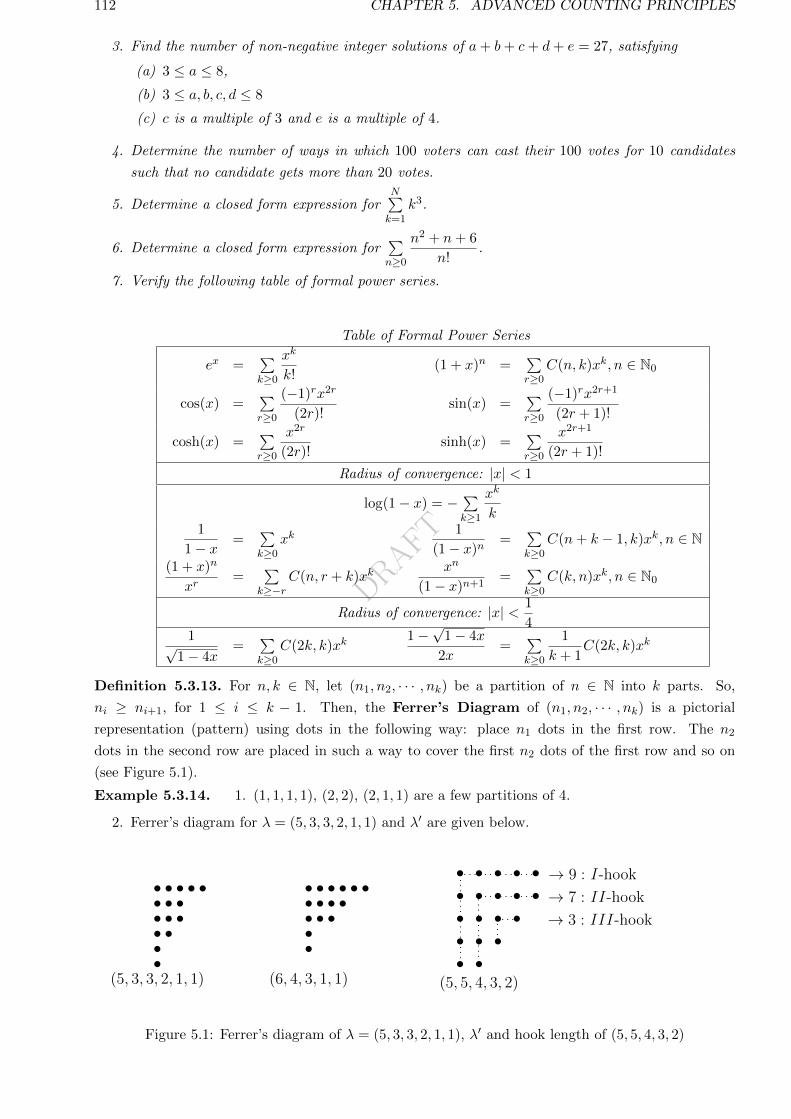
DRAFT


3. Find the number of non-negative integer solutions of a+ b+ c+ d+ e = 27, satisfying

(a) 3 ≤ a ≤ 8,

(b) 3 ≤ a, b, c, d ≤ 8

(c) c is a multiple of 3 and e is a multiple of 4.

4. Determine the number of ways in which 100 voters can cast their 100 votes for 10 candidates

such that no candidate gets more than 20 votes.

5. Determine a closed form expression forN∑k=1

k3.

6. Determine a closed form expression for∑n≥0

n2 + n+ 6

n!.

7. Verify the following table of formal power series.

Table of Formal Power Series

ex =∑k≥0

xk

k!(1 + x)n =

∑r≥0

C(n, k)xk, n ∈ N0

cos(x) =∑r≥0

(−1)rx2r

(2r)!sin(x) =

∑r≥0

(−1)rx2r+1

(2r + 1)!

cosh(x) =∑r≥0

x2r

(2r)!sinh(x) =

∑r≥0

x2r+1

(2r + 1)!

Radius of convergence: |x| < 1

log(1− x) = − ∑k≥1

xk

k1

1− x =∑k≥0

xk1

(1− x)n=

∑k≥0

C(n+ k − 1, k)xk, n ∈ N(1 + x)n

xr=

∑k≥−r

C(n, r + k)xkxn

(1− x)n+1=

∑k≥0

C(k, n)xk, n ∈ N0

Radius of convergence: |x| < 1

41√

1− 4x=

∑k≥0

C(2k, k)xk1−√

1− 4x

2x=

∑k≥0

1

k + 1C(2k, k)xk

Definition 5.3.13. For n, k ∈ N, let (n1, n2, · · · , nk) be a partition of n ∈ N into k parts. So,

ni ≥ ni+1, for 1 ≤ i ≤ k − 1. Then, the Ferrer’s Diagram of (n1, n2, · · · , nk) is a pictorial

representation (pattern) using dots in the following way: place n1 dots in the first row. The n2

dots in the second row are placed in such a way to cover the first n2 dots of the first row and so on

(see Figure 5.1).

Example 5.3.14. 1. (1, 1, 1, 1), (2, 2), (2, 1, 1) are a few partitions of 4.

2. Ferrer’s diagram for λ = (5, 3, 3, 2, 1, 1) and λ′ are given below.

• • •• •• • •• • •• •••

(5, 3, 3, 2, 1, 1)

• • •• • •• • • •• • •••

(6, 4, 3, 1, 1)

• • •• •• • • ••• • • •• • •• •

(5, 5, 4, 3, 2)

→ 9 : I-hook

→ 7 : II-hook

→ 3 : III-hook

1

Figure 5.1: Ferrer’s diagram of λ = (5, 3, 3, 2, 1, 1), λ′ and hook length of (5, 5, 4, 3, 2)

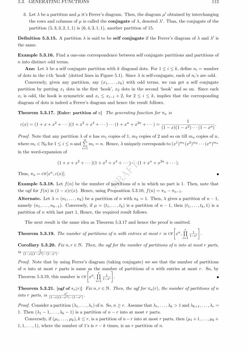
DRAFT


3. Let λ be a partition and µ it’s Ferrer’s diagram. Then, the diagram µ′ obtained by interchanging

the rows and columns of µ is called the conjugate of λ, denoted λ′. Thus, the conjugate of the

partition (5, 3, 3, 2, 1, 1) is (6, 4, 3, 1, 1), another partition of 15.

Definition 5.3.15. A partition λ is said to be self conjugate if the Ferrer’s diagram of λ and λ′ is

the same.

Example 5.3.16. Find a one-one correspondence between self conjugate partitions and partitions of

n into distinct odd terms.

Ans: Let λ be a self conjugate partition with k diagonal dots. For 1 ≤ i ≤ k, define ni = number

of dots in the i-th ‘hook’ (dotted lines in Figure 5.1). Since λ is self-conjugate, each of ni’s are odd.

Conversely, given any partition, say (x1, . . . , xk) with odd terms, we can get a self conjugate

partition by putting x1 dots in the first ‘hook’, x2 dots in the second ‘hook’ and so on. Since each

xi is odd, the hook is symmetric and xi ≤ xi−1 + 2, for 2 ≤ i ≤ k, implies that the corresponding

diagram of dots is indeed a Ferrer’s diagram and hence the result follows.

Theorem 5.3.17. [Euler: partition of n] The generating function for πn is

ε(x) = (1 + x+ x2 + · · · )(1 + x2 + x4 + · · · ) · · · (1 + xn + x2n + · · · ) =1

(1− x)(1− x2) · · · (1− xn).

Proof. Note that any partition λ of n has m1 copies of 1, m2 copies of 2 and so on till mn copies of n,

wheremi ∈ N0 for 1 ≤ i ≤ n andn∑i=1

mi = n. Hence, λ uniquely corresponds to (x1)m1(x2)m2 · · · (xn)mn

in the word-expansion of

(1 + x+ x2 + · · · )(1 + x2 + x4 + · · · ) · · · (1 + xn + x2n + · · · ).

Thus, πn = cf[xn, ε(x)].

Example 5.3.18. Let f(n) be the number of partitions of n in which no part is 1. Then, note that

the ogf for f(n) is (1− x)ε(x). Hence, using Proposition 5.3.10, f(n) = πn − πn−1.Alternate. Let λ = (n1, . . . , nk) be a partition of n with nk = 1. Then, λ gives a partition of n− 1,

namely (n1, . . . , nk−1). Conversely, if µ = (t1, . . . , tk) is a partition of n − 1, then (t1, . . . , tk, 1) is a

partition of n with last part 1, Hence, the required result follows.

The next result is the same idea as Theorem 5.3.17 and hence the proof is omitted.

Theorem 5.3.19. The number of partitions of n with entries at most r is cf

[xn,

r∏i=1

11−xi

].

Corollary 5.3.20. Fix n, r ∈ N. Then, the ogf for the number of partitions of n into at most r parts,

is 1(1−x)(1−x2)···(1−xr) .

Proof. Note that by using Ferrer’s diagram (taking conjugate) we see that the number of partitions

of n into at most r parts is same as the number of partitions of n with entries at most r. So, by

Theorem 5.3.19, this number is cf

[xn,

r∏i=1

11−xi

].

Theorem 5.3.21. [ogf of πn(r)] Fix n, r ∈ N. Then, the ogf for πn(r), the number of partitions of n

into r parts, is xr

(1−x)(1−x2)···(1−xr) .

Proof. Consider a partition (λ1, . . . , λr) of n. So, n ≥ r. Assume that λ1, . . . , λk > 1 and λk+1, . . . , λr =

1. Then (λ1 − 1, . . . , λk − 1) is a partition of n− r into at most r parts.

Conversely, if (µ1, . . . , µk), k ≤ r, is a partition of n− r into at most r parts, then (µ1 + 1, . . . , µk +

1, 1, . . . , 1), where the number of 1’s is r − k times, is an r partition of n.

DRAFT


Thus, the number of r partitions of n is the same as the number of partitions of n − r with at

most r parts. Thus, by Corollary 5.3.20 the required number is cf[xn−r, 1

(1−x)(1−x2)···(1−xr)

]. Hence,

the ogf for πn(r) isxr

(1− x)(1− x2) · · · (1− xr) .

Exercise 5.3.22. 1. For n, r ∈ N, prove that πn(r) is the number of partitions of n+C(r, 2) into

r unequal parts.

2. Let P,M ⊆ N and f(n) be the number of partitions of n where parts are from P and multiplicities

are from M . Find the generating function for the numbers f(n).

Theorem 5.3.23. Suppose there are k types of objects.

1. If there is an unlimited supply of each object, then the egf of the number of r-permutations is

ekx.

2. If there are mi copies of i-th object, then the egf of the number of r-permutations is(1 + x+

x2

2!+ · · ·+ xm1

m1!

)· · ·(

1 + x+x2

2!+ · · ·+ xmk

mk!

).

3. Moreover, n!S(r, n) is the coefficient of xr

r! in (ex − 1)n.

Proof. Part 1: Since there are unlimited supply of each object, the egf for each object corresponds to

ex = 1 + x+ · · ·+ xn

n!+ · · · . Hence, the required result follows.

Part 2: Argument is similar to that of Part 1 and is omitted.

Part 3: Recall that n!S(r, n) is the number of surjections from 1, 2, . . . , r to X = s1, · · · , sn.Each surjection can be viewed as word of length r of elements of X, with each si appearing at least

once. Thus, we need a selection of ki ∈ N copies of si, withn∑i=1

ki = r. Also, by Theorem 4.1.23, this

number equals C(r; k1, · · · , kn). Hence,

n!S(r, n) = r!cf

[xr,

(x+

x2

2!+x3

3!+ · · ·

)n]= cf

[xr

r!, (ex − 1)n

].

Example 5.3.24. 1. In how many ways can you get Rs 2007 using denominations 1, 10, 100, 1000

only?

Ans: cf

[x2007,

1

(1− x)(1− x10)(1− x100)(1− x1000)

].

2. If we use at most 9 of each denomination in Part 1, then this number is

cf

[x2007,

(9∑i=1

xi

)(9∑i=1

x10i

)(9∑i=1

x100i

)(9∑i=1

x1000i

)]= cf

[x2007,

1− x100001− x

]= 1.

3. Every natural number has a unique base-r representation (r ≥ 2). Note that Part 2 corresponds

to the case r = 10.

4. Consider n integers k1 < k2 < · · · < kn with gcd(k1, . . . , kn) = 1. Then, the number of natural

numbers not having a partition using k1, . . . , kn is finite. Determining the largest such integer

(Frobenius number) is the coin problem/ money changing problem. The general problem is

NP-hard. No closed form formula is known for n > 3.

Notice!

Some times we have a way to obtain a recurrence relation from the generating function.

This is important and hence study the next example carefully.

DRAFT


Example 5.3.25. 1. Suppose F =1

(1− x)(1− x10)(1− x100)(1− x1000) =∑n≥0

anxn. Then, tak-

ing log and differentiating, we get

F ′ = F

[1

1− x +10x9

1− x10 +100x99

1− x100 +1000x999

1− x1000].

So,

nan = cf[xn−1, F ′

]= cf

[xn−1, F

[1

1− x +10x9

1− x10 +100x99

1− x100 +1000x999

1− x1000]]

=n∑k=1

an−kbk,

where

bk = cf

[xk−1,

[1

1− x +10x9

1− x10 +100x99

1− x100 +1000x999

1− x1000]]

=

1 if 10 - k11 if 10|k, 100 - k111 if 100|k, 1000 - k1111 else.

2. We know that limn→∞

n∑k=1

1k =∞. What about lim

n→∞

n∑k=1

1pk

, where pk is the k-th prime?

Ans: For n > 1, let sn =n∑k=1

1k . Then, note that

sn ≤(

1 +1

2+

1

4+ · · ·

)(1 +

1

3+

1

9+ · · ·

)· · ·(

1 +1

pn+

1

p2n+ · · ·

)=

n∏k=1

(1 +1

pk − 1).

Thus,

log sn ≤ log

(n∏k=1

(1 +1

pk − 1)

)≤

n∑k=1

log(1 +1

pk − 1) ≤

n∑k=1

1

pk − 1≤ 1 +

n−1∑k=1

1

pk.

As n→∞, we see that limn→∞

n∑i=1

1pi

=∞ as limn→∞

log sn =∞.

3. Let X be the set of natural numbers with only prime divisors 2, 3, 5, 7. Then,

1 +∑n∈X

1

n= (1 +

1

2+

1

4+ · · · )(1 +

1

3+

1

9+ · · · ) · · · (1 +

1

7+

1

49+ · · · ) =

2

1

3

2

5

4

7

6=

35

8.

Exercise 5.3.26. 1. Let σ(n) =∑d|nd, for n ∈ N. Then, prove that nπn =

n∑k=1

πn−kσ(k).

2. A Durfee square is the largest square in a Ferrer’s diagram. Find the generating function for the

number of self conjugate partitions of n with a fixed size k of Durfee square. Hence, show that

(1 + x)(1 + x3) · · · = 1 +

∞∑k=1

xk2

(1− x2)(1− x4) · · · (1− x2k) .

3. Show that the number of partitions of n into distinct terms (each term is distinct) is the same

as the number of partitions of n into odd terms (each term is odd).

4. Find the number of r-digit binary numbers that can be formed using an even number of 0’s and

an even number of 1’s.

5. Find the egf of the number of words of size r using A,B,C,D,E,

(a) if the word has all the letters and the letter A appears an even many times.

(b) if the word has all the letters and the first letter of the word appears an even number of

times.

DRAFT


6. A permutation σ of 1, 2, . . . , n is said to be connected if there does not exist k, 1 ≤ k < n

such that σ takes 1, 2, . . . , k to itself. Let cn denote the number of connected permutations of

1, 2, . . . , n (put c0 = 0), then show that

n∑k=1

ck(n− k)! = n!.

Hence, derive the relationship between the generating functions of (n!) and (cn).

7. Let f(n, r) be the number of partitions of n where each part repeats less than r times. Let g(n, r)

be the number of partition of n where no part is divisible by r. Show that f(n, r) = g(n, r).

8. Find the number of 9-sequences that can be formed using 0, 1, 2, 3 in each case.

(a) The sequence has an even number of 0’s.

(b) The sequence has an odd number of 1’s and an even number of 0’s.

(c) No digit appears exactly twice.

5.4 Recurrence Relation

Definition 5.4.1. A recurrence relation is a way of recursively defining the terms of a sequence

as a function of preceding terms together with certain initial conditions.

Example 5.4.2. an = 3 + 2an−1 for n ≥ 1 with the initial condition a0 = 1 is a recurrence relation.

Note that it completely determines the sequence (an) = 1, 5, 13, 29, 61, . . ..

Definition 5.4.3. For a sequence (an), the first difference d(an) is an − an−1. The k-th differ-

ence dk(an) = dk−1(an) − dk−1(an−1). A difference equation is an equation involving an and its

differences.

Example 5.4.4. 1. an − d2(an) = 5 is a difference equation. But, note that it doesn’t give a

recurrence relation as we don’t have any initial condition(s).

2. Every recurrence relation can be expressed as a difference equation. The difference equation

corresponding to the recurrence relation an = 3 + 2an−1 is an = 3 + 2(an − d(an)).

Definition 5.4.5. A solution of a recurrence relation is a function u(n), generally denoted by un,

satisfying the recurrence relation.

Example 5.4.6. 1. un = 2n+2 − 3 is a solution of an = 3 + 2an−1 with a0 = 1.

2. The Fibonacci sequence is given by an = an−1 + an−2 for n ≥ 2 with a0 = 0, a1 = 1. Use(1+√5

2

)2= 3+

√5

2 and(1−√5

2

)2= 3−

√5

2 to verify that an =1√5

((1+√5

2

)n−(1−√5

2

)n)is a

solution of the recurrence relation that defines the Fibonacci sequence.

Definition 5.4.7. A recurrence relation is a linear nonhomogeneous recurrence relation with

constant coefficients (LNHRRCC) of order r if, for a known function f

an = c1an−1 + · · ·+ cran−r + f(n), where ci ∈ R for 1 ≤ i ≤ r, cr 6= 0. (5.3)

If f = 0, then Equation (5.3) is homogeneous and is called the associated linear homogeneous

recurrence relation with constant coefficients (LHRRCC).

Theorem 5.4.8. For k ∈ N, let fi, 1 ≤ i ≤ k be known functions. Consider the k LNHRRCC

an = c1an−1 + · · ·+ cran−r + fi(n) for i = 1, . . . , k, (5.4)

DRAFT

5.4. RECURRENCE RELATION 117

with the same set of initial conditions. If ui(n), for 1 ≤ i ≤ k, is a solution of the i-th recurrence

then,

an = c1an−1 + · · ·+ cran−r +k∑i=1

αifi(n) (5.5)

under the same set of initial conditions hask∑i=1

αiui(n) as it’s solution.

Proof. The proof is left as an exercise for the reader.

Definition 5.4.9. Consider a LHRRCC an = c1an−1 + · · · + cran−r with cr 6= 0. If an = xn is a

solution, then either x = 0 or x is a root of

xr − c1xr−1 − · · · − cr = 0. (5.6)

Equation (5.6) is called the characteristic equation of the given LHRRCC. If x1, . . . , xr are the roots of

Equation (5.6), then an = xni (and hence an =r∑i=1

αixni for αi ∈ R) is a solution of the given LHRRCC.

Theorem 5.4.10. [General solution: distinct roots] If the roots xi, i = 0, . . . , r − 1 of Equation (5.6)

are distinct, then every solution u(n) is a linear combination of xni . Moreover, the solution is unique

if we are given r consecutive initial conditions.

Proof. Let u(n) be any solution. Then, we need to show that there exist αi ∈ R, 0 ≤ i ≤ r − 1, such

that u(n) =r−1∑i=0

αixni . Substituting n = 0, 1, . . . , r − 1, one obtains the linear system

u(0)u(1)

...u(r − 1)

=

1 · · · 1x0 · · · xr−1

. . .

xr−10 · · · xr−1r−1

α0

α1...

αr−1

in the unknowns αi’s 0 ≤ i ≤ r−1. Since the above r×r matrix (commonly known as the Vandermonde

matrix) is invertible, there exist α0, . . . , αr−1, such that u(m) =r−1∑i=0

αixmi for 0 ≤ m ≤ r − 1. Hence,

we have proved the result for the first r values of u(n). So, let us assume that the result is true for

n < k. Then, by definition

u(k) =

r∑j=1

cjh(k − j) =

r∑j=1

cj

r−1∑i=0

αixk−ji =

r−1∑i=0

αi

r∑j=1

cjxk−ji =

r−1∑i=0

αixki ,

as for n = k, xki is a solution of Equation (5.6). Thus, by PMI, u(n) =r−1∑i=0

αixni for all n. The

uniqueness is left as an exercise for the reader.

Example 5.4.11. 1. Solve an − 4an−2 = 0 for n ≥ 2 with a0 = 1 and a1 = 1.

Ans: Note that ±2 are the roots of the characteristic equation, x2 − 4 = 0. As the roots

are distinct, the general solution is an = α(−2)n + β2n for α, β ∈ R. The initial conditions

give α + β = 1 and 2β − 2α = 1. Hence, α = 14 , β = 3

4 . Thus, the unique solutions is

an = 2n−2(3 + (−1)n

).

2. Solve an = 3an−1 + 4an−2 for n ≥ 2 with a0 = 1 and a1 = c, a constant.

Ans: Note that −1 and 4 are the roots of the characteristic equation, x2 − 3x − 4 = 0. As

the roots are distinct, the general solution is an = α(−1)n + β4n for α, β ∈ R. Now, the initial

conditions imply α = 4−c5 andβ = 1+c

5 . Thus, the unique general solution is

DRAFT


(a) an =(4− c)(−1)n

5+

(1 + c)4n

5, if c 6= 4.

(b) an = 4n, if c = 4.

3. Solve the Fibonacci recurrence an = an−1 + an−2 with initial conditions a0 = 0, a1 = 1.

Ans: In this case, note that the roots of the characteristic equation, x2 − x− 1 = 0, are 1±√5

2 .

As the roots are distinct, the general solution is an = α(1+√5

2

)n+ β(1−√5

2

)nfor α, β ∈ R. Now,

using the initial conditions, we get α = 1√5, β = −α. Hence, the required solution is

an = α(1 +

√5

2

)n+ β

(1−√

5

2

)n=

1√5

[(1 +√

5

2

)n−(

1−√

5

2

)n]. (5.7)

Theorem 5.4.12. [General solution: multiple roots] Let t is a root of Equation (5.6) of multiplicity

s. Then, u(n) = tn(s−1∑i=0

αini

), for αi ∈ R, 0 ≤ i ≤ s− 1, is a solution (basic solution). In general,

if ti is a root of Equation (5.6) with multiplicity si), for i = 1, . . . , k, then every solution is a sum of

the k basic solutions.

Proof. It is given that t is a zero of the polynomial F = xr − c1xr−1 − · · · − cr of multiplicity s. Put

G0 = xn−rF = xn − c1xn−1 − · · · − crxn−r and G1 = xG′0, G2 = xG′1, . . ., Gs−1 = xG′s−2. Then, each

of G0, G1, . . . , Gs−1 has a zero at t. That is, for i = 0, 1, . . . , s− 1, we have

Gi(t) = tnni − c1tn−1(n− 1)i − . . .− crtn−r(n− r)i = 0.

Thus, for any choice of αi ∈ R, 0 ≤ i ≤ s− 1, if one defines P (k) =s−1∑i=1

kiαi, for k ≥ 0 then

s−1∑i=0

αiGi(t) = tnP (n)− c1tn−1P (n− 1)− · · · − crtn−rP (n− r) = 0.

Thus, by definition u(n)−c1u(n−1)−· · ·−cru(n−r) = 0. Hence, u(n) is a solution of the LHRRCC.

The other part of the proof is left for the reader.

Example 5.4.13. Suppose that an LHRRCC has roots 2, 2, 3, 3, 3. Then, the general solution is given

by 2n(α1 + nα2) + 3n(β1 + nβ2 + n2β3).

Theorem 5.4.14. [LNHRRCC] Consider the LNHRRCC in Equation (5.3) and let un be a general

solution to the associated LHRRCC. If vn is a particular solution of the LNHRRCC, then an = un+vn

is a general solution of the LNHRRCC.

Proof. The proof is left for the reader.

Notice!

No general algorithm are there to solve an LNHRRCC. If f(n) = an or nk or a linear combination

of these, then a particular solution can be easily obtained.

Obtaining particular solution after knowledge of the characteristic roots.

1. If f(n) = an and a is not a root of Equation (5.3), then vn = can.

2. If f(n) = an and a is a root of Equation (5.3) of multiplicity t, then vn = cntan.

3. If f(n) = nk and 1 is not a root of Equation (5.3), then use vn = c0 + c1n+ · · ·+ cknk.

4. If f(n) = nk and 1 is a root of Equation (5.3) of multiplicity t, then

vn = nt(c0 + c1n+ · · ·+ cknk).

DRAFT

5.5. GENERATING FUNCTION FROM RECURRENCE RELATION 119

Example 5.4.15. 1. Let an = 3an−1 + 2n for n ≥ 1 with a0 = 1.

Ans: Observe that 3 is the characteristic root of the associated LHRRCC (an = 3an−1). Thus,

the general solution of LHRRCC is un = 3nα. Note that 1 is not a characteristic root and hence a

particular solution is a+nb, where a and b are to be computed using a+nb = 3(a+(n−1)b)+2n.

This gives a = −32 and b = −1. Hence, an = 3nα− n− 3

2. Using a0 = 1, check that α =

5

2.

2. Let an = 3an−1 − 2an−2 + 3(5)n for n ≥ 3 with a1 = 1, a2 = 2.

Ans: Observe that 1 and 2 are the characteristic roots of the associated LHRRCC (an =

3an−1 − 2an−2). Thus, the general solution of the LHRRCC is un = α1n + β2n. Note that 5 is

not a characteristic root and thus, vn = c5n is a particular solution of LNHRRCC if and only if

c5n = 3c5n−1 − 2c5n−2 + 3(5)n. That is, if and only if c = 25/4. Hence, the general solution of

LNHRRCC equals an = α+β2n+(25/4)5n, where compute α and β using the initial conditions.

3. In the above take f(n) = 3(2n). Then, we see that with c(2)n as a choice for a particular

solution, we will have 4c = 6c− 2c+ 12, an absurd statement. But, with the choice cn(2)n, we

have 4nc = 6(n−1)c−2(n−2)c+12, implying c = 6. Hence, the general solution of LNHRRCC

is an = α+ β2n + 6n2n, where compute α and β using the initial conditions.

5.5 Generating Function from Recurrence Relation

Sometimes we can find a solution to the recurrence relation using the generating function of an.

Example 5.5.1. 1. Consider an = 2an−1 + 1, a0 = 1.

Ans: Let F (x) = a0 + a1x+ · · · be the generating function for ai. Then,

F = 1 +

∞∑i=1

aixi = 1 +

∞∑i=1

(2ai−1 + 1)xi =

∞∑i=0

xi + 2x

∞∑i=0

aixi =

1

1− x + 2xF.

Hence, F = 1(1−x)(1−2x) = 2

1−2x − 11−x . Thus, an = cf[xn, F ] = 2n+1 − 1.

2. Find the ogf F for the Fibonacci recurrence relation an = an−1 + an−2, a0 = 0, a1 = 1.

Ans: Define F (x) =∑n≥0

anxn =

∑n≥1

anxn. Then using the recurrence relation, we have

F (x) =∑n≥0

anxn = x+

∑n≥2

(an−1 + an−2)xn = x+ (x+ x2)F (x).

So, F (x) = x1−x−x2 . Let α = 1+

√5

2 and β = 1−√5

2 . Then it can be checked that (1−αx)(1−βx) =

1− x− x2 and

F (x) =1√5

( 1

1− αx −1

1− βx)

=1√5

∑n≥0

αnxn −∑n≥0

βnxn

.

Therefore, an = cf[xn, F (x)] =1√5

∑n≥0

(αn − βn), which equals Equation (5.7).

The next result follows using a small calculation and hence the proof is left for the reader.

Theorem 5.5.2. [Obtaining generating function from recurrence relation] Consider the r-th order

LHRRCC given by

an = c1an−1 + · · ·+ cran−r with initial conditions ai = Ai for i = 0, 1, . . . , r − 1. (5.8)

DRAFT


Then, the generating function of Equation (5.8) equals

r−1∑i=0

Aixi − c1x

r−2∑i=0

Aixi − c2x

2r−3∑i=0

Aixi − · · · − cr−1xr−1A0

1 − c1x − · · · − crxr.

Example 5.5.3. 1. Find the ogf for the Catalan numbers Cn’s.

Ans: Let g(x) = 1 +∑n≥1

Cnxn, where Cn = C(2n,n)

n+1 = 2(2n−1)n+1 Cn−1 with C0 = 1. Then,

g(x)− 1 =∑n≥1

Cnxn =

∑n≥1

2(2n− 1)

n+ 1Cn−1xn

=∞∑n=1

4n+ 4

n+ 1Cn−1xn +

∞∑n=1

−6

n+ 1Cn−1xn = 4xg(x) +

−6

x

x∫0

tg(t)dt.

So, [g(x) − 1 − 4xg(x)]x = −6x∫0

tg(t)dt. Now, we differentiate with respect to x to get x(1 −4x)g′ + (1− 2x)g = 1. To solve the ode, we first observe that∫

1− 2x

x(1− 4x)=

∫ [1

x+

2

1− 4x

]= ln

(x√

1− 4x

).

Thus, the integrating factor of the given ode is x√1−4x . Hence, the ode can be re-written as

g(x)′x√

1− 4x+ g(x)

1− 2x

(1− 4x)3/2=

1

(1− 4x)3/2⇔ d

dx

[g(x)

x√1− 4x

]=

1

(1− 4x)3/2.

Hence, g(x) x√1−4x = 1

2√1−4x + C, where C ∈ R. Or, equivalently 2xg(x) = 1 + 2C

√1− 4x.

Note that C = −12 as C0 = lim

x→0g(x) = 1. Thus, the ogf of the Catalan numbers is

g(x) =1−√

1− 4x

2x.

Alternate. Recall that Cn is the number of representations of the product of n + 1 square

matrices of the same size, using n pairs of brackets. From such a representation, remove the

leftmost and the rightmost brackets to obtain the product of two representations of the form:

A1(A2 · · ·An+1), (A1A2)(A3 · · ·An+1), · · · , (A1 · · ·Ak)(Ak+1 · · ·An+1), · · · , (A1 · · ·An)An+1.

Hence, we see that

Cn = C0Cn−1 + C1Cn−2 + · · ·+ Cn−1C0. (5.9)

Thus, if we define g(x) =∞∑n=0

Cnxn, then for n ≥ 1,

cf[xn−1, g(x)2

]= cf

xn−1,( ∞∑n=0

Cnxn

)2 =

n−1∑i=0

CiCn−1−i = Cn using Equation (5.9).

That is, cf[xn, xg(x)2

]= Cn. Hence, g(x) = 1 + xg(x)2. Solving for g(x), we get

g(x) =1

2

(1

x±√

1

x2− 4

x

)=

1±√

1− 4x

2x.

As the function g is continuous (being a power series in the domain of convergence) and

limx→0

g(x) = C0 = 1, it follows that

g(x) =1−√

1− 4x

2x.

DRAFT


2. Fix r ∈ N and let (an) be a sequence with a0 = 1 andn∑k=0

akan−k = C(n + r, r), for all n ≥ 1.

Determine an.

Ans: Let g(x) =∑n≥0

anxn. Then, note that C(n+ r, r) = c(n+ (r + 1)− 1, n). Hence,

g(x)2 =∑n≥0

(n∑k=0

akan−k

)xn =

∑n≥0

C(n+ r, r)xn =∑n≥0

C(n+ r, n)xn =1

(1− x)r+1.

Hence, an = cf[xn, 1

(1−x)(r+1)/2

]. For example, for r = 2 (see Equation (4.2)),

an = (−1)nC(−3/2, n) =3 · 5 · 7 · · · (2n+ 1)

2n n!=

(2n+ 1)!

22nn!n!.

3. Determine the sequence f(n,m) | n,m ∈ N0 which satisfies f(n, 0) = 1 for all n ≥ 0, f(0,m) =

0 for all m > 0 and

f(n,m) = f(n− 1,m) + f(n− 1,m− 1) for (n,m) 6= (0, 0). (5.10)

Ans: For n ≥ 1, define Fn(x) =∑m≥0

f(n,m)xm = 1 +∑m≥1

f(n,m)xm. Then F1(x) = 1 + x and

for n ≥ 2,

Fn(x) =∑m≥0

f(n,m)xm = 1 +∑m≥1

(f(n− 1,m) + f(n− 1,m− 1))xm

= 1 +∑m≥1

f(n− 1,m)xm +∑m≥1

f(n− 1,m− 1)xm

= Fn−1(x) + xFn−1(x) = (1 + x)Fn−1(x) = · · · = (1 + x)n

as F1(x) = 1 + x. Thus,

f(n,m) = cf[xm, (1 + x)n] =

C(n,m) if 0 ≤ m ≤ n0 if m > n.

Alternate. For m ≥ 1, define Gm(y) =∑n≥0

f(n,m)yn =∑n≥1

f(n,m)yn. Then, G1(y) =

y

(1− y)2and for m ≥ 2, Equation (5.10) gives

Gm(y) =∑n≥1

f(n,m)yn =∑n≥1

(f(n− 1,m) + f(n− 1,m− 1)) yn

=∑n≥1

f(n− 1,m)yn +∑n≥1

f(n− 1,m− 1)yn

= yGm(y) + yGm−1(y).

Therefore, Gm(y) =y

1− yGm−1(y). As G1(y) =y

(1− y)2, one has Gm(y) =

ym

(1− y)m+1. Thus,

f(n,m) = cf

[yn,

ym

(1− y)m+1

]= cf

[yn−m,

1

(1− y)m+1

]=

C(n,m) if 0 ≤ m ≤ n0 if m > n.

4. Determine the sequence S(n,m) | n,m ∈ N0 which satisfy S(0, 0) = 1, S(n,m) = 0 if either

m = 0 or n = 0 but not both and

S(n,m) = mS(n− 1,m) + S(n− 1,m− 1), (n,m) 6= (0, 0). (5.11)

DRAFT


Ans: For n ≥ 1, define Gm(y) =∑n≥0

S(n,m)yn =∑n≥1

S(n,m)yn. Then, G1(y) = y1−y and for

m ≥ 1, Equation (5.11) gives

Gm(y) =∑n≥0

S(n,m)yn =∑n≥1

(mS(n− 1,m) + S(n− 1,m− 1)) yn

= m∑n≥1

S(n− 1,m)yn +∑n≥1

S(n− 1,m− 1)yn

= myGm(y) + yGm−1(y).

Therefore, Gm(y) =y

1−myGm−1(y). As G1(y) =y

1− y , one has

Gm(y) =ym

(1− y)(1− 2y) · · · (1−my)= ym

m∑k=1

αk1− ky , (5.12)

where αk =(−1)m−kkm

k! (m− k)!, for 1 ≤ k ≤ m. Thus,

S(n,m) = cf

[yn, ym

m∑k=1

αk1− ky

]=

m∑k=1

cf

[yn−m,

αk1− ky

]

=

m∑k=1

αkkn−m =

m∑k=1

(−1)m−kkn

k! (m− k)!(5.13)

=1

m!

m∑k=1

(−1)m−kknC(m, k) =1

m!

m∑k=1

(−1)k(m− k)nC(m, k).

Therefore, S(n,m) =1

m!

m∑k=1

(−1)k(m− k)nC(m, k).

This identity is generally known as the Stirling’s Identity.

Observation.

(a) Let us consider Hn(x) =∑m≥0

S(n,m)xm. Then, verify that Hn(x) = (x + xD)n · 1 as

H0(x) = 1. Therefore, H1(x) = x, H2(x) = x + x2, · · · . Thus, we don’t have a single

expression for Hn(x) which gives the value of S(n,m)’s. But, it helps in showing that

S(n,m), for fixed n ∈ N, first increase and then decrease (commonly called unimodal).

The same holds for the sequence of binomial coefficients C(n,m),m = 0, 1, . . . , n.(b) As there is no restriction on n.m ∈ N0, Equation (5.13) is also valid for n < m. But, we

know that S(n,m) = 0, whenever n < m. Hence, we get the following identity,

m∑k=1

(−1)m−k kn−1

(k − 1)! (m− k)!= 0 whenever n < m.

5. For n ∈ N, the n-th Bell number, denoted b(n), is the number of partitions of 1, 2, . . . , n.Thus, b(n) =

n∑m=1

S(n,m), for n ≥ 1 and b(0) = 1. Hence, for n ≥ 1,

b(n) =n∑

m=1

S(n,m) =∑m≥1

S(n,m) =∑m≥1

m∑k=1

(−1)m−k kn−1

(k − 1)! (m− k)!

=∑k≥1

kn

k!

∑m≥k

(−1)m−k

(m− k)!=

1

e

∑k≥1

kn

k!=

1

e

∑k≥0

kn

k!as 0n = 0 for n 6= 0. (5.14)

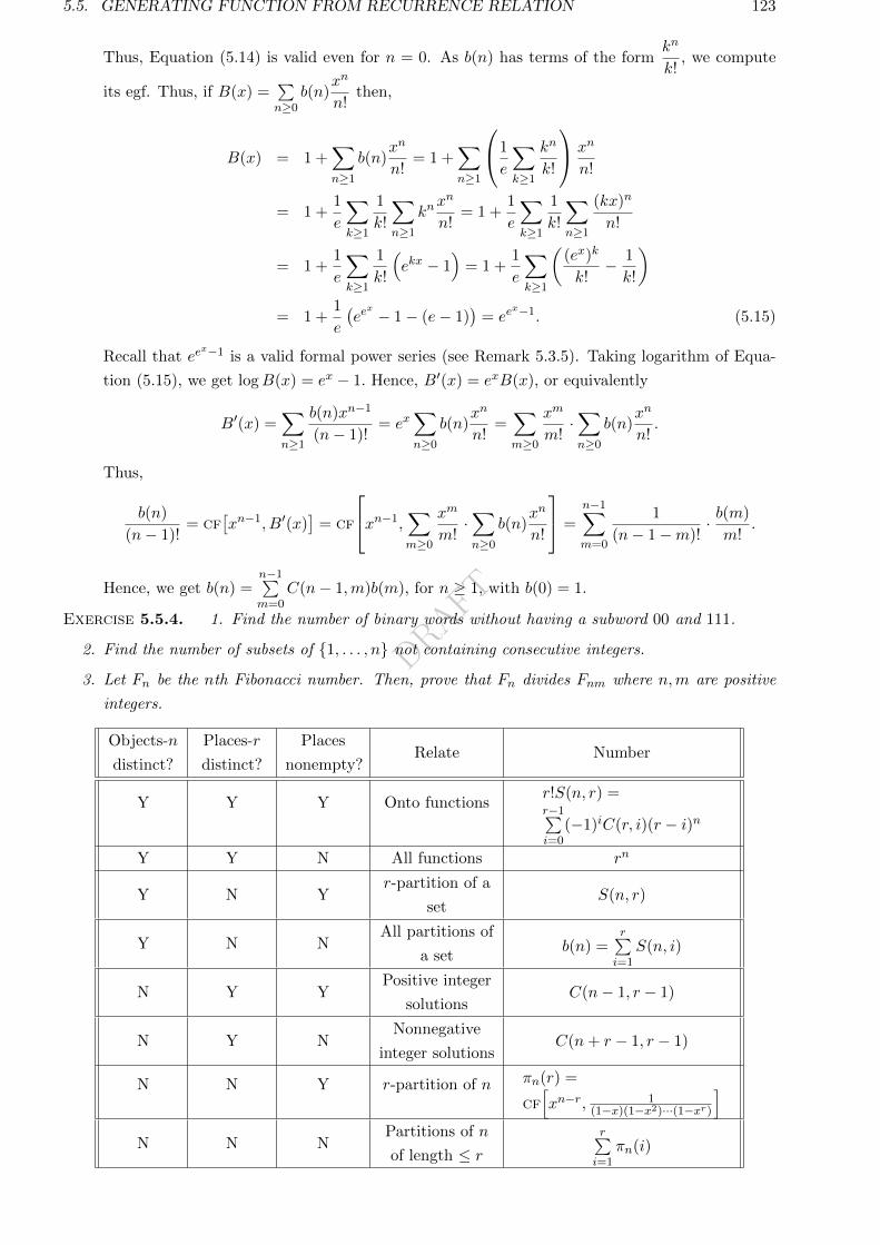
DRAFT


Thus, Equation (5.14) is valid even for n = 0. As b(n) has terms of the formkn

k!, we compute

its egf. Thus, if B(x) =∑n≥0

b(n)xn

n!then,

B(x) = 1 +∑n≥1

b(n)xn

n!= 1 +

∑n≥1

1

e

∑k≥1

kn

k!

xn

n!

= 1 +1

e

∑k≥1

1

k!

∑n≥1

knxn

n!= 1 +

1

e

∑k≥1

1

k!

∑n≥1

(kx)n

n!

= 1 +1

e

∑k≥1

1

k!

(ekx − 1

)= 1 +

1

e

∑k≥1

((ex)k

k!− 1

k!

)= 1 +

1

e

(eex − 1− (e− 1)

)= ee

x−1. (5.15)

Recall that eex−1 is a valid formal power series (see Remark 5.3.5). Taking logarithm of Equa-

tion (5.15), we get logB(x) = ex − 1. Hence, B′(x) = exB(x), or equivalently

B′(x) =∑n≥1

b(n)xn−1

(n− 1)!= ex

∑n≥0

b(n)xn

n!=∑m≥0

xm

m!·∑n≥0

b(n)xn

n!.

Thus,

b(n)

(n− 1)!= cf

[xn−1, B′(x)

]= cf

xn−1,∑m≥0

xm

m!·∑n≥0

b(n)xn

n!

=

n−1∑m=0

1

(n− 1−m)!· b(m)

m!.

Hence, we get b(n) =n−1∑m=0

C(n− 1,m)b(m), for n ≥ 1, with b(0) = 1.

Exercise 5.5.4. 1. Find the number of binary words without having a subword 00 and 111.

2. Find the number of subsets of 1, . . . , n not containing consecutive integers.

3. Let Fn be the nth Fibonacci number. Then, prove that Fn divides Fnm where n,m are positive

integers.

Objects-n

distinct?

Places-r

distinct?

Places

nonempty?Relate Number

Y Y Y Onto functionsr!S(n, r) =r−1∑i=0

(−1)iC(r, i)(r − i)n

Y Y N All functions rn

Y N Yr-partition of a

setS(n, r)

Y N NAll partitions of

a setb(n) =

r∑i=1

S(n, i)

N Y YPositive integer

solutionsC(n− 1, r − 1)

N Y NNonnegative

integer solutionsC(n+ r − 1, r − 1)

N N Y r-partition of n πn(r) =

cf[xn−r, 1

(1−x)(1−x2)···(1−xr)

]N N N

Partitions of n

of length ≤ rr∑i=1

πn(i)

DRAFT


Exercise 5.5.5. 1. In a particular semester 6 students took admission in our PhD program. There

were 9 professors who were willing to supervise these students. As a rule ‘a student can have

either one or two supervisors’. In how many ways can we allocate supervisors to these students

if all the ‘willing professors’ are to be allocated? What if we have an additional condition that

exactly one supervisor gets to supervise two students?

2. (a) Prove combinatorially that, for n ≥ 2, we have Dn = (n− 1)(Dn−1 +Dn−2).

(b) Use Part (a) to show that the exponential generating function of Dn ise−x

1− x .

3. My friend says that he has n ≥ 2 subsets of 1, 2, . . . , 14 each of which has size 6. Give a value

of n so that we can guarantee ‘some two of his subsets have 3 elements in common’, without

seeing his collection’? What is the smallest possible value of n?

4. Find the number of words of size 12 made using letters from A,B,C in which ‘BCA’ does

not appear (as a consecutive subword). For example: ABCABCCCCCBA has an appearance of

‘BCA’ but BCCABCCABCCA does not.

5. Find the number of 8 letter words made using alphabets from A,B,C,D in which 3 consecutive

letters are not allowed to be the same.

6. We have 3 blue bags, 4 red bags and 5 green bags. We have many balls of each of the colors blue,

red and green. Fill in the blank with the smallest positive integer.

If we distribute balls (without seeing the colors) into these bags, then one of the following

must happen:

(a) a blue bag contains 3 blue balls or 4 red balls or 5 green balls

(b) a red bag contains 3 blue balls or 5 red balls or 7 green balls

(c) a green bag contains 3 blue balls or 6 red balls or 9 green balls

7. We have an integer polynomial f(x). Fill in the blank with the smallest positive integer.

If f(x) = 2009 has many distinct integer roots, then f(x) = 9002 cannot have an integer

root.

8. (a) In how many ways can one distribute 10 identical chocolates among 10 students?

(b) In how many ways can one distribute 10 distinct chocolates among 10 students?

(c) In how many ways can one distribute 10 distinct chocolates among 10 students so that each

receives one?

(d) In how many ways can one distribute 15 distinct chocolates among 10 students so that each

receives at least one?

(e) In how many ways can one distribute 10 out of 15 distinct chocolates among 10 students so

that each receives one?

(f) In how many ways can one distribute 15 distinct chocolates among 10 students so that each

receives at most three?

(g) In how many ways can one distribute 15 distinct chocolates among 10 students so that each

receives at least one and at most three?

(h) In how many ways can one distribute 15 identical chocolates among 10 students so that

each receives at most three?

9. (a) In how many ways can one carry 15 distinct objects with 10 identical bags? Answer using

S(n, r).

(b) In how many ways can one carry 15 distinct objects in 10 identical bags with no empty bag?

Answer using S(n, r).

DRAFT


(c) In how many ways can one carry 15 distinct objects in 10 identical bags with each bag

containing at most three objects?

(d) In how many ways can one carry 15 identical objects in 10 identical bags?

(e) In how many ways can one carry 15 identical objects in 10 identical bags with no empty

bag?

(f) In how many ways can one carry 15 identical objects in 20 identical bags?

10. What is the number of integer solutions of x+ y + z = 10, with x ≥ −1, y ≥ −2 and z ≥ −3?

11. Is the number of solutions of x+ y+ z = 10 in non-negative multiples of 12 (x, y, z are allowed to

be 0, 1/2, 1, 3/2, . . .) at most four times the number of non-negative integer solutions of x+y+z =

10?

12. How many words of length 8 can be formed using the English alphabets, where each letter can

appear at most twice? Give answer using generating function.

13. Let p1, . . . , pn, n ≥ 2 be distinct prime numbers. Consider the set p1, . . . , pn, p21, . . . , p2n. In

how many ways can we partition the set into subsets of size two such that no prime is in the

same subset containing its square?

14. What is the value of15∑k=0

(−1)kC(15, k)(15− k)5?

15. Give your answers using generating function.

(a) What is the number of partitions of n with entries at most r?

(b) What is the number of partitions of n with at most r parts?

(c) What is the number of partitions of n with exactly r parts (πn(r))?

(d) What is the number of partitions of n+ C(r, 2) with r distinct parts?

(e) What is the number of partitions of n with distinct entries?

(f) What is the number of partitions of n with entries odd?

(g) What is the number of partitions of n with distinct odd entries?

(h) What is the number of partitions of n which are self conjugate?

16. How many words of length 15 are there using the letters A,B,C,D,E such that each letter must

appear in the word and A appears an even number of times? Give your answers using generating

function.

17. The characteristic roots of a LHRRCC are 2, 2, 2, 3, 3. What is the form of the general solution?

18. Consider the LNHRRCC an = c1an−1 + · · ·+ cran−r + 5n. Give a particular solution.

19. Obtain the ogf for an, where an = 2an−1 − an−2 + 2n, a0 = 0, a1 = 1.

20. Solve the recurrence relation an = 2an−1 − an−2 + 2n + 5, a0 = 0, a1 = 1.

21. My class has n CSE, m MSC and r MC students. Suppose that t copies of the same book are

to be distributed so that each branch gets at least s. In how many ways can this be done, if each

student gets at most one? In how many ways can this be done, without the previous restriction?

Answer only using generating function.

Exercise 5.5.6. 1. My class has n CSE, m MSC and r MC students. Suppose that t distinct

books are to be distributed so that each branch gets at least s. In how many ways can this be

done, if each student gets at most one? In how many ways can this be done, without the previous

restriction? Answer only using generating function.

DRAFT


2. My class has N students. Assume that, to conduct an exam, we have M identical answer

scripts. In how many ways can we distribute the answer scripts so that each student gets at least

2. Answer only using generating function.

3. My class has N students. Assume that, for an exam, we have M questions; each student answers

all the questions in an order decided by him/her (for example one can follow 1, 2, · · · ,M and

another can follow M,M − 1, · · · , 1). In how many ways can it happen that some three or more

students have followed the same order? Answer only using generating function.

4. When ‘Freshers Welcome’ was organized 11 teachers went to attend. There were 4 types of soft

drinks available. In how many ways a total of 18 glasses of soft drinks can be served to them, in

general? Answer only using generating function.

DRAFT

Chapter 6

Introduction to Logic

6.1 Propositional Logic

We study logic to differentiate between valid and invalid arguments. An argument is a set of state-

ments which has two parts: premise and conclusion. There can be many statements in the premise.

Conclusion is just one statement. An argument has the structure

premise: Statement1, . . ., Statementk; therefore conclusion: Statementc.

Consider the following examples.

• Statement1: If today is Monday, then Mr. X gets Rs. 5.

Statement2: Today is Monday.

Statementc: Therefore, Mr. X gets Rs. 5 (statementc).


Statement2: Mr. X gets Rs. 5.

Statementc: Therefore, today is Monday.


Statement2: Today is Tuesday.

Statementc: Therefore, Mr. X gets Rs. 5.


Statement2: Today is Tuesday.

Statementc: Therefore, Mr. X does not get Rs. 5.

We understand that the first one is a valid argument, whereas the next three are not. In order to

differentiate between valid and invalid argument, we need to analyze an argument. And in order to

do that, we first have to understand ‘what is a statement’. A simple statement is an expression which

is either false or true but not both. We create complex statements from the old ones by using ‘and’,

‘or’ and ‘not’.

For example, ‘today is Monday’ is a statement. ‘Today is Tuesday’ is also a statement. ‘Today is

Monday and today is Tuesday’ is also a statement. ‘Today is not Monday’ is also a statement.

One way to analyze an argument is by writing it using symbols. The following definition captures

the notion of a ‘statement’.

Definition 6.1.1. 1. [Atomic formulae and truth values] Consider a nonempty finite set of

symbols F . We shall call an element of F as an atomic formula (also called atomic variable).

(These are our simple statements). The truth value of each element in F is exactly one of T

(for TRUE) and F (for FALSE). Normally, we use symbols p, q, p1, p2, . . . for atomic formulae.

127

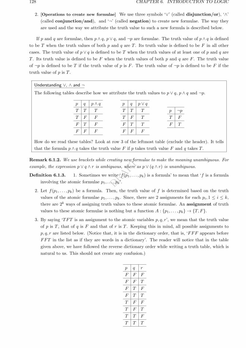
DRAFT

128 CHAPTER 6. INTRODUCTION TO LOGIC

2. [Operations to create new formulae] We use three symbols ‘∨’ (called disjunction/or), ‘∧’

(called conjunction/and), and ‘¬’ (called negation) to create new formulae. The way they

are used and the way we attribute the truth value to such a new formula is described below.

If p and q are formulae, then p ∧ q, p ∨ q, and ¬p are formulae. The truth value of p ∧ q is defined

to be T when the truth values of both p and q are T . Its truth value is defined to be F in all other

cases. The truth value of p ∨ q is defined to be T when the truth values of at least one of p and q are

T . Its truth value is defined to be F when the truth values of both p and q are F . The truth value

of ¬p is defined to be T if the truth value of p is F . The truth value of ¬p is defined to be F if the

truth value of p is T .

Understanding ∨, ∧ and ¬The following tables describe how we attribute the truth values to p ∨ q, p ∧ q and ¬p.

p q p ∧ qT T T

T F F

F T F

F F F

p q p ∨ qT T T

T F T

F T T

F F F

p ¬pT F

F T

How do we read these tables? Look at row 3 of the leftmost table (exclude the header). It tells

that the formula p ∧ q takes the truth value F if p takes truth value F and q takes T .

Remark 6.1.2. We use brackets while creating new formulae to make the meaning unambiguous. For

example, the expression p ∨ q ∧ r is ambiguous, where as p ∨ (q ∧ r) is unambiguous.

Definition 6.1.3. 1. Sometimes we write ‘f(p1, . . . , pk) is a formula’ to mean that ‘f is a formula

involving the atomic formulae p1, . . . , pk’.

2. Let f(p1, . . . , pk) be a formula. Then, the truth value of f is determined based on the truth

values of the atomic formulae p1, . . . , pk. Since, there are 2 assignments for each pi, 1 ≤ i ≤ k,

there are 2k ways of assigning truth values to these atomic formulae. An assignment of truth

values to these atomic formulae is nothing but a function A : p1, . . . , pk → T, F.

3. By saying ‘TFT is an assignment to the atomic variables p, q, r’, we mean that the truth value

of p is T , that of q is F and that of r is T . Keeping this in mind, all possible assignments to

p, q, r are listed below. (Notice that, it is in the dictionary order, that is, ‘FFF appears before

FFT in the list as if they are words in a dictionary’. The reader will notice that in the table

given above, we have followed the reverse dictionary order while writing a truth table, which is

natural to us. This should not create any confusion.)

p q r

F F F

F F T

F T F

F T T

T F F

T F T

T T F

T T T

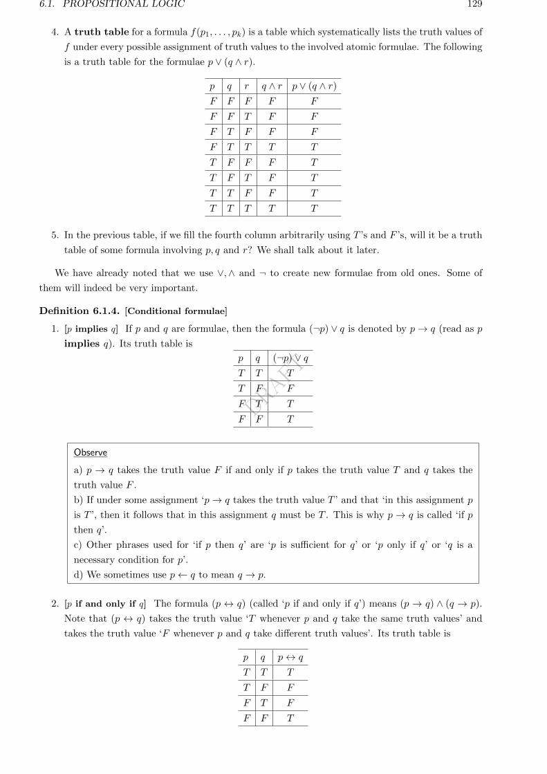
DRAFT

6.1. PROPOSITIONAL LOGIC 129

4. A truth table for a formula f(p1, . . . , pk) is a table which systematically lists the truth values of

f under every possible assignment of truth values to the involved atomic formulae. The following

is a truth table for the formulae p ∨ (q ∧ r).

p q r q ∧ r p ∨ (q ∧ r)F F F F F

F F T F F

F T F F F

F T T T T

T F F F T

T F T F T

T T F F T

T T T T T

5. In the previous table, if we fill the fourth column arbitrarily using T ’s and F ’s, will it be a truth

table of some formula involving p, q and r? We shall talk about it later.

We have already noted that we use ∨,∧ and ¬ to create new formulae from old ones. Some of

them will indeed be very important.

Definition 6.1.4. [Conditional formulae]

1. [p implies q] If p and q are formulae, then the formula (¬p) ∨ q is denoted by p→ q (read as p

implies q). Its truth table is

p q (¬p) ∨ qT T T

T F F

F T T

F F T

Observe

a) p → q takes the truth value F if and only if p takes the truth value T and q takes the

truth value F .

b) If under some assignment ‘p→ q takes the truth value T ’ and that ‘in this assignment p

is T ’, then it follows that in this assignment q must be T . This is why p→ q is called ‘if p

then q’.

c) Other phrases used for ‘if p then q’ are ‘p is sufficient for q’ or ‘p only if q’ or ‘q is a

necessary condition for p’.

d) We sometimes use p← q to mean q → p.

2. [p if and only if q] The formula (p ↔ q) (called ‘p if and only if q’) means (p → q) ∧ (q → p).

Note that (p ↔ q) takes the truth value ‘T whenever p and q take the same truth values’ and

takes the truth value ‘F whenever p and q take different truth values’. Its truth table is

p q p↔ q

T T T

T F F

F T F

F F T

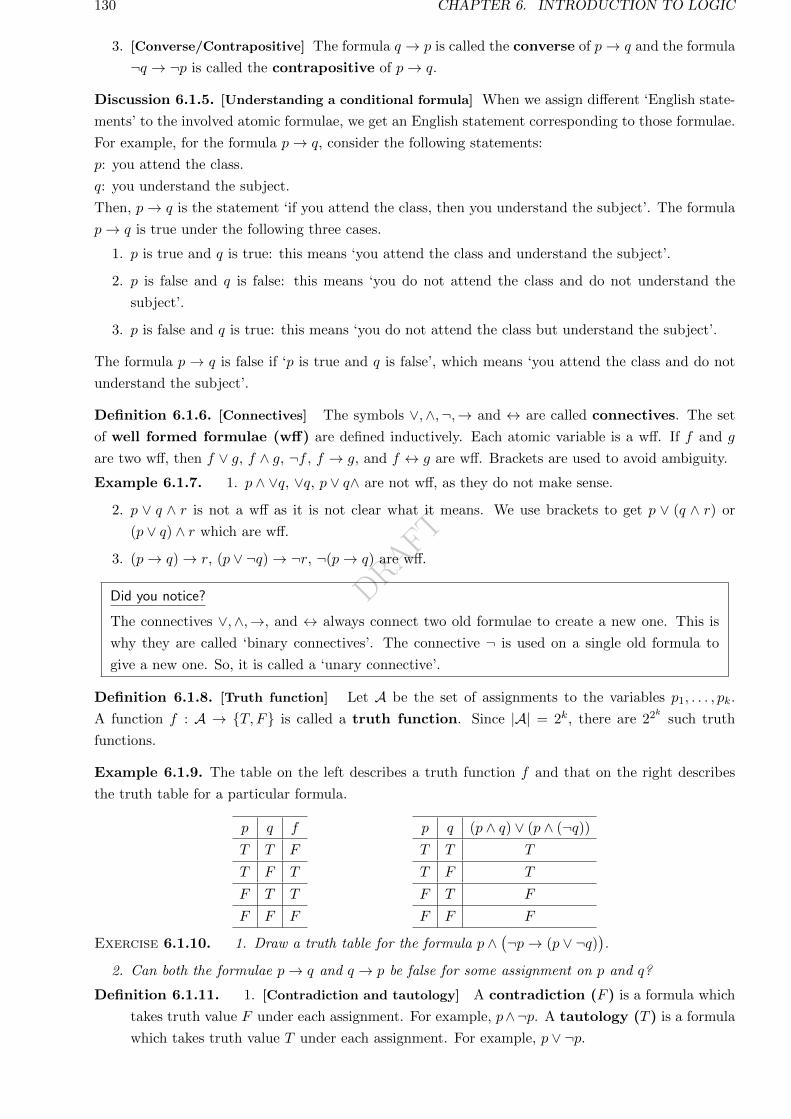
DRAFT


3. [Converse/Contrapositive] The formula q → p is called the converse of p→ q and the formula

¬q → ¬p is called the contrapositive of p→ q.

Discussion 6.1.5. [Understanding a conditional formula] When we assign different ‘English state-

ments’ to the involved atomic formulae, we get an English statement corresponding to those formulae.

For example, for the formula p→ q, consider the following statements:

p: you attend the class.

q: you understand the subject.

Then, p→ q is the statement ‘if you attend the class, then you understand the subject’. The formula

p→ q is true under the following three cases.

1. p is true and q is true: this means ‘you attend the class and understand the subject’.

2. p is false and q is false: this means ‘you do not attend the class and do not understand the

subject’.

3. p is false and q is true: this means ‘you do not attend the class but understand the subject’.

The formula p → q is false if ‘p is true and q is false’, which means ‘you attend the class and do not

understand the subject’.

Definition 6.1.6. [Connectives] The symbols ∨,∧,¬,→ and ↔ are called connectives. The set

of well formed formulae (wff) are defined inductively. Each atomic variable is a wff. If f and g

are two wff, then f ∨ g, f ∧ g, ¬f , f → g, and f ↔ g are wff. Brackets are used to avoid ambiguity.

Example 6.1.7. 1. p ∧ ∨q, ∨q, p ∨ q∧ are not wff, as they do not make sense.

2. p ∨ q ∧ r is not a wff as it is not clear what it means. We use brackets to get p ∨ (q ∧ r) or

(p ∨ q) ∧ r which are wff.

3. (p→ q)→ r, (p ∨ ¬q)→ ¬r, ¬(p→ q) are wff.

Did you notice?

The connectives ∨,∧,→, and ↔ always connect two old formulae to create a new one. This is

why they are called ‘binary connectives’. The connective ¬ is used on a single old formula to

give a new one. So, it is called a ‘unary connective’.

Definition 6.1.8. [Truth function] Let A be the set of assignments to the variables p1, . . . , pk.

A function f : A → T, F is called a truth function. Since |A| = 2k, there are 22k

such truth

functions.

Example 6.1.9. The table on the left describes a truth function f and that on the right describes

the truth table for a particular formula.

p q f

T T F

T F T

F T T

F F F

p q (p ∧ q) ∨ (p ∧ (¬q))T T T

T F T

F T F

F F F

Exercise 6.1.10. 1. Draw a truth table for the formula p ∧(¬p→ (p ∨ ¬q)

).

2. Can both the formulae p→ q and q → p be false for some assignment on p and q?

Definition 6.1.11. 1. [Contradiction and tautology] A contradiction (F ) is a formula which

takes truth value F under each assignment. For example, p∧¬p. A tautology (T ) is a formula

which takes truth value T under each assignment. For example, p ∨ ¬p.

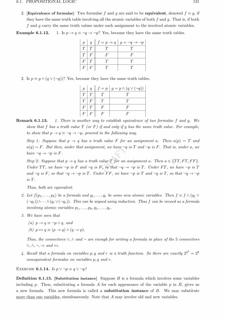
DRAFT


2. [Equivalence of formulae] Two formulae f and g are said to be equivalent, denoted f ≡ g, if

they have the same truth table involving all the atomic variables of both f and g. That is, if both

f and g carry the same truth values under each assignment to the involved atomic variables.

Example 6.1.12. 1. Is p→ q ≡ ¬q → ¬p? Yes, because they have the same truth tables.

p q f = p→ q g = ¬q → ¬pT T T T

T F F F

F T T T

F F T T

2. Is p ≡ p ∧ (q ∨ (¬q))? Yes, because they have the same truth tables.

p q f = p g = p ∧ (q ∨ (¬q))T T T T

T F T T

F T F F

F F F F

Remark 6.1.13. 1. There is another way to establish equivalence of two formulae f and g. We

show that f has a truth value T (or F ) if and only if g has the same truth value. For example,

to show that p→ q ≡ ¬q → ¬p, proceed in the following way.

Step 1: Suppose that p → q has a truth value F for an assignment a. Then a(p) = T and

a(q) = F . But then, under that assignment, we have ¬q is T and ¬p is F . That is, under a, we

have ¬q → ¬p is F .

Step 2: Suppose that p→ q has a truth value T for an assignment a. Then a ∈ TT, FT, FF.Under TT , we have ¬p is F and ¬q is F , so that ¬q → ¬p is T . Under FT , we have ¬p is T

and ¬q is F , so that ¬q → ¬p is T . Under FF , we have ¬p is T and ¬q is T , so that ¬q → ¬pis T .

Thus, both are equivalent.

2. Let f(p1, . . . , pk) be a formula and q1, . . . , qr be some new atomic variables. Then f ≡ f ∧ (q1 ∨(¬q1))∧· · ·∧(qr∨(¬qr)). This can be argued using induction. Thus f can be viewed as a formula

involving atomic variables p1, . . . , pk, q1, . . . , qr.

3. We have seen that

(a) p→ q ≡ ¬p ∨ q, and

(b) p↔ q ≡ (p→ q) ∧ (q → p).

Thus, the connectives ∨,∧ and ¬ are enough for writing a formula in place of the 5 connectives

∨,∧,¬,→ and ↔.

4. Recall that a formula on variables p, q and r is a truth function. So there are exactly 223

= 28

nonequivalent formulae on variables p, q and r.

Exercise 6.1.14. Is p ∨ ¬p ≡ q ∨ ¬q?

Definition 6.1.15. [Substitution instance] Suppose B is a formula which involves some variables

including p. Then, substituting a formula A for each appearance of the variable p in B, gives us

a new formula. This new formula is called a substitution instance of B. We may substitute

more than one variables, simultaneously. Note that A may involve old and new variables.

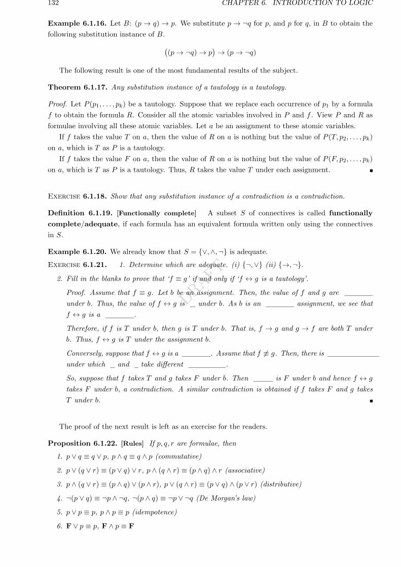
DRAFT


Example 6.1.16. Let B: (p→ q)→ p. We substitute p→ ¬q for p, and p for q, in B to obtain the

following substitution instance of B.((p→ ¬q)→ p

)→ (p→ ¬q)

The following result is one of the most fundamental results of the subject.

Theorem 6.1.17. Any substitution instance of a tautology is a tautology.

Proof. Let P (p1, . . . , pk) be a tautology. Suppose that we replace each occurrence of p1 by a formula

f to obtain the formula R. Consider all the atomic variables involved in P and f . View P and R as

formulae involving all these atomic variables. Let a be an assignment to these atomic variables.

If f takes the value T on a, then the value of R on a is nothing but the value of P (T, p2, . . . , pk)

on a, which is T as P is a tautology.

If f takes the value F on a, then the value of R on a is nothing but the value of P (F, p2, . . . , pk)

on a, which is T as P is a tautology. Thus, R takes the value T under each assignment.

Exercise 6.1.18. Show that any substitution instance of a contradiction is a contradiction.

Definition 6.1.19. [Functionally complete] A subset S of connectives is called functionally

complete/adequate, if each formula has an equivalent formula written only using the connectives

in S.

Example 6.1.20. We already know that S = ∨,∧,¬ is adequate.

Exercise 6.1.21. 1. Determine which are adequate. (i) ¬,∨ (ii) →,¬.2. Fill in the blanks to prove that ‘f ≡ g’ if and only if ‘f ↔ g is a tautology’.

Proof. Assume that f ≡ g. Let b be an assignment. Then, the value of f and g are

under b. Thus, the value of f ↔ g is under b. As b is an assignment, we see that

f ↔ g is a .

Therefore, if f is T under b, then g is T under b. That is, f → g and g → f are both T under

b. Thus, f ↔ g is T under the assignment b.

Conversely, suppose that f ↔ g is a . Assume that f 6≡ g. Then, there is

under which and take different .

So, suppose that f takes T and g takes F under b. Then is F under b and hence f ↔ g

takes F under b, a contradiction. A similar contradiction is obtained if f takes F and g takes

T under b.

The proof of the next result is left as an exercise for the readers.

Proposition 6.1.22. [Rules] If p, q, r are formulae, then

1. p ∨ q ≡ q ∨ p, p ∧ q ≡ q ∧ p (commutative)

2. p ∨ (q ∨ r) ≡ (p ∨ q) ∨ r, p ∧ (q ∧ r) ≡ (p ∧ q) ∧ r (associative)

3. p ∧ (q ∨ r) ≡ (p ∧ q) ∨ (p ∧ r), p ∨ (q ∧ r) ≡ (p ∨ q) ∧ (p ∨ r) (distributive)

4. ¬(p ∨ q) ≡ ¬p ∧ ¬q, ¬(p ∧ q) ≡ ¬p ∨ ¬q (De Morgan’s law)

5. p ∨ p ≡ p, p ∧ p ≡ p (idempotence)

6. F ∨ p ≡ p, F ∧ p ≡ F

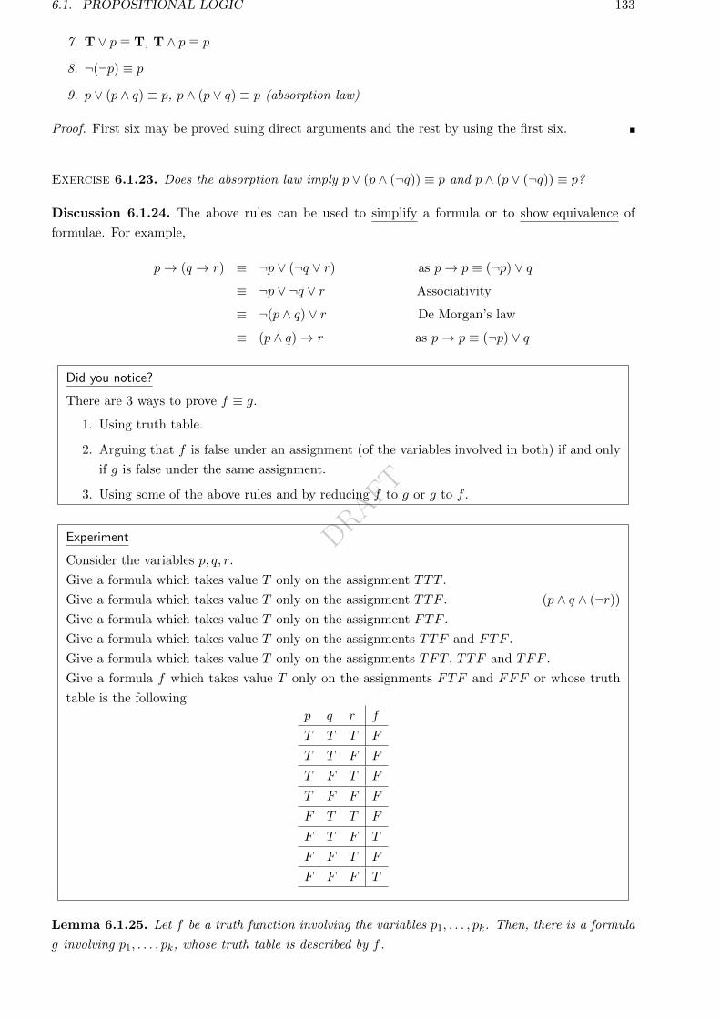
DRAFT


7. T ∨ p ≡ T, T ∧ p ≡ p

8. ¬(¬p) ≡ p

9. p ∨ (p ∧ q) ≡ p, p ∧ (p ∨ q) ≡ p (absorption law)

Proof. First six may be proved suing direct arguments and the rest by using the first six.

Exercise 6.1.23. Does the absorption law imply p ∨ (p ∧ (¬q)) ≡ p and p ∧ (p ∨ (¬q)) ≡ p?

Discussion 6.1.24. The above rules can be used to simplify a formula or to show equivalence of

formulae. For example,

p→ (q → r) ≡ ¬p ∨ (¬q ∨ r) as p→ p ≡ (¬p) ∨ q≡ ¬p ∨ ¬q ∨ r Associativity

≡ ¬(p ∧ q) ∨ r De Morgan’s law

≡ (p ∧ q)→ r as p→ p ≡ (¬p) ∨ q

Did you notice?

There are 3 ways to prove f ≡ g.

1. Using truth table.

2. Arguing that f is false under an assignment (of the variables involved in both) if and only

if g is false under the same assignment.

3. Using some of the above rules and by reducing f to g or g to f .

Experiment

Consider the variables p, q, r.

Give a formula which takes value T only on the assignment TTT .

Give a formula which takes value T only on the assignment TTF . (p ∧ q ∧ (¬r))Give a formula which takes value T only on the assignment FTF .

Give a formula which takes value T only on the assignments TTF and FTF .

Give a formula which takes value T only on the assignments TFT , TTF and TFF .

Give a formula f which takes value T only on the assignments FTF and FFF or whose truth

table is the following

p q r f

T T T F

T T F F

T F T F

T F F F

F T T F

F T F T

F F T F

F F F T

Lemma 6.1.25. Let f be a truth function involving the variables p1, . . . , pk. Then, there is a formula

g involving p1, . . . , pk, whose truth table is described by f .

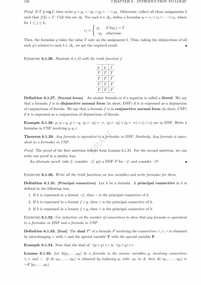
DRAFT


Proof. If T /∈ rng f , then write q = p1 ∧ ¬p1 ∧ p2 ∧ · · · ∧ pk. Otherwise, collect all those assignments b

such that f(b) = T . Call this set A1. For each b ∈ A1, define a formulae q = r1 ∧ r2 ∧ · · · ∧ rk, where

for 1 ≤ j ≤ k,

rj =

pj if b(pj) = T

¬pj otherwise.

Then, the formulae q takes the value T only on the assignment b. Thus, taking the disjunctions of all

such q’s related to each b ∈ A1, we get the required result.

Exercise 6.1.26. Illustrate 6.1.25 with the truth function f

p q f

T T T

T F T

F T F

F F F

Definition 6.1.27. [Normal forms] An atomic formula or it’s negation is called a literal. We say

that a formula f is in disjunctive normal form (in short, DNF) if it is expressed as a disjunction

of conjunctions of literals. We say that a formula f is in conjunctive normal form (in short, CNF)

if it is expressed as a conjunction of disjunctions of literals.

Example 6.1.28. p, p ∨ q, p ∨ ¬q, (p ∧ ¬q) ∨ ¬r, (p ∧ ¬q) ∨ (q ∧ ¬r) ∨ (r ∧ s) are in DNF. Write 5

formulae in CNF involving p, q, r.

Theorem 6.1.29. Any formula is equivalent to a formulae in DNF. Similarly, Any formula is equiv-

alent to a formulae in CNF.

Proof. The proof of the first assertion follows from Lemma 6.1.25. For the second assertion, we can

write one proof in a similar way.

An alternate proof: take f , consider ¬f , get a DNF P for ¬f , and consider ¬P .

Exercise 6.1.30. Write all the truth functions on two variables and write formulae for them.

Definition 6.1.31. [Principal connectives] Let h be a formula. A principal connective in h is

defined in the following way.

1. If h is expressed in a format ¬f , then ¬ is the principal connective of h.

2. If h is expressed in a format f ∨ g, then ∨ is the principal connective of h.

3. If h is expressed in a format f ∧ g, then ∧ is the principal connective of h.

Exercise 6.1.32. Use induction on the number of connectives to show that any formula is equivalent

to a formulae in DNF and a formula in CNF.

Definition 6.1.33. [Dual] The dual P ∗ of a formula P involving the connectives ∨,∧,¬ is obtained

by interchanging ∨ with ∧ and the special variable T with the special variable F.

Example 6.1.34. Note that the dual of ¬(p ∨ q) ∧ r is ¬(p ∧ q) ∨ r.

Lemma 6.1.35. Let A(p1, . . . , pk) be a formula in the atomic variables pi involving connectives

∨,∧ and ¬. If A(¬p1, . . . ,¬pk) is obtained by replacing pi with ¬pi in A, then A(¬p1, . . . ,¬pk) ≡¬A∗(p1, . . . , pk).

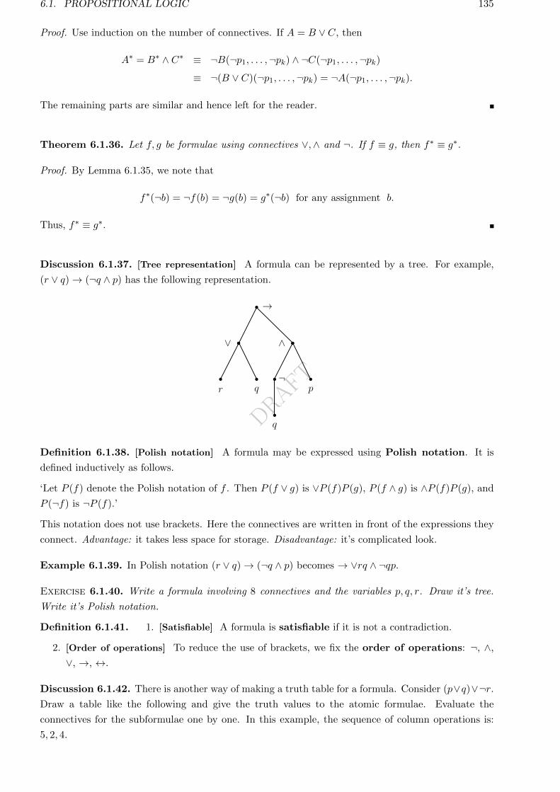
DRAFT


Proof. Use induction on the number of connectives. If A = B ∨ C, then

A∗ = B∗ ∧ C∗ ≡ ¬B(¬p1, . . . ,¬pk) ∧ ¬C(¬p1, . . . ,¬pk)≡ ¬(B ∨ C)(¬p1, . . . ,¬pk) = ¬A(¬p1, . . . ,¬pk).

The remaining parts are similar and hence left for the reader.

Theorem 6.1.36. Let f, g be formulae using connectives ∨,∧ and ¬. If f ≡ g, then f∗ ≡ g∗.

Proof. By Lemma 6.1.35, we note that

f∗(¬b) = ¬f(b) = ¬g(b) = g∗(¬b) for any assignment b.

Thus, f∗ ≡ g∗.

Discussion 6.1.37. [Tree representation] A formula can be represented by a tree. For example,

(r ∨ q)→ (¬q ∧ p) has the following representation.

p

q

r q

∨ ∧

¬

→

Definition 6.1.38. [Polish notation] A formula may be expressed using Polish notation. It is

defined inductively as follows.

‘Let P (f) denote the Polish notation of f . Then P (f ∨ g) is ∨P (f)P (g), P (f ∧ g) is ∧P (f)P (g), and

P (¬f) is ¬P (f).’

This notation does not use brackets. Here the connectives are written in front of the expressions they

connect. Advantage: it takes less space for storage. Disadvantage: it’s complicated look.

Example 6.1.39. In Polish notation (r ∨ q)→ (¬q ∧ p) becomes → ∨rq ∧ ¬qp.

Exercise 6.1.40. Write a formula involving 8 connectives and the variables p, q, r. Draw it’s tree.

Write it’s Polish notation.

Definition 6.1.41. 1. [Satisfiable] A formula is satisfiable if it is not a contradiction.

2. [Order of operations] To reduce the use of brackets, we fix the order of operations: ¬, ∧,

∨, →, ↔.

Discussion 6.1.42. There is another way of making a truth table for a formula. Consider (p∨q)∨¬r.Draw a table like the following and give the truth values to the atomic formulae. Evaluate the

connectives for the subformulae one by one. In this example, the sequence of column operations is:

5, 2, 4.

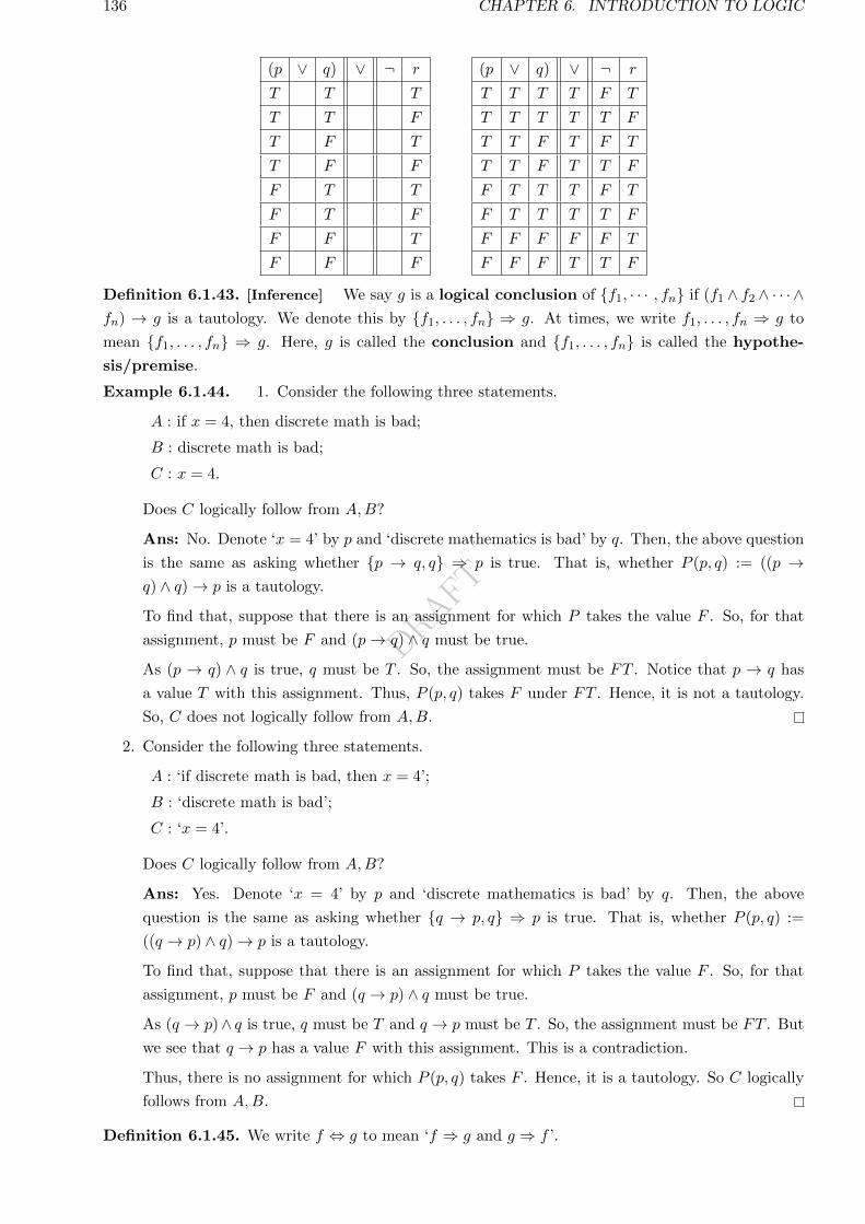
DRAFT


(p ∨ q) ∨ ¬ r

T T T

T T F

T F T

T F F

F T T

F T F

F F T

F F F

(p ∨ q) ∨ ¬ r

T T T T F T

T T T T T F

T T F T F T

T T F T T F

F T T T F T

F T T T T F

F F F F F T

F F F T T F

Definition 6.1.43. [Inference] We say g is a logical conclusion of f1, · · · , fn if (f1 ∧ f2 ∧ · · · ∧fn) → g is a tautology. We denote this by f1, . . . , fn ⇒ g. At times, we write f1, . . . , fn ⇒ g to

mean f1, . . . , fn ⇒ g. Here, g is called the conclusion and f1, . . . , fn is called the hypothe-

sis/premise.

Example 6.1.44. 1. Consider the following three statements.

A : if x = 4, then discrete math is bad;

B : discrete math is bad;

C : x = 4.

Does C logically follow from A,B?

Ans: No. Denote ‘x = 4’ by p and ‘discrete mathematics is bad’ by q. Then, the above question

is the same as asking whether p → q, q ⇒ p is true. That is, whether P (p, q) := ((p →q) ∧ q)→ p is a tautology.

To find that, suppose that there is an assignment for which P takes the value F . So, for that

assignment, p must be F and (p→ q) ∧ q must be true.

As (p → q) ∧ q is true, q must be T . So, the assignment must be FT . Notice that p → q has

a value T with this assignment. Thus, P (p, q) takes F under FT . Hence, it is not a tautology.

So, C does not logically follow from A,B.

2. Consider the following three statements.

A : ‘if discrete math is bad, then x = 4’;

B : ‘discrete math is bad’;

C : ‘x = 4’.

Does C logically follow from A,B?

Ans: Yes. Denote ‘x = 4’ by p and ‘discrete mathematics is bad’ by q. Then, the above

question is the same as asking whether q → p, q ⇒ p is true. That is, whether P (p, q) :=

((q → p) ∧ q)→ p is a tautology.

To find that, suppose that there is an assignment for which P takes the value F . So, for that

assignment, p must be F and (q → p) ∧ q must be true.

As (q → p)∧ q is true, q must be T and q → p must be T . So, the assignment must be FT . But

we see that q → p has a value F with this assignment. This is a contradiction.

Thus, there is no assignment for which P (p, q) takes F . Hence, it is a tautology. So C logically

follows from A,B.

Definition 6.1.45. We write f ⇔ g to mean ‘f ⇒ g and g ⇒ f ’.

DRAFT


Did you notice?

Let f, g, h be some formulae. Then f, g ⇒ h means that ‘whenever f and g are T , h is also T ’.

That is, ‘if f and g are T under an assignment, then h is T under that assignment’. Thus ‘f ⇔ g’

is the same as ‘f ≡ g’.

Example 6.1.46. 1. Show that α→ β, β → γ, γ → δ ⇒ α→ δ.

Ans: Suppose α → δ is F . Then α is T and δ is F . Assume that all the propositions in the

hypothesis are true. As δ is F and γ → δ is T , γ must be F . Continuing, we get α is F , a

contradiction.

2. Determine validity of the argument.

The meeting can take place if all members are informed in advance and there is quorum (a

minimum number of members are present). There is a quorum if at least 15 members are

present. Members would have been informed in advance if there was no postal strike. Therefore,

if the meeting was canceled, then either there were fewer than 15 members present or there was

a postal strike.

A : Let us denote the different statements with symbols, say

m: the meeting takes place;

a: all members are informed;

f : at least fifteen members are present;

q: the meeting had quorum;

p: there was a postal strike.

So, we reformulate the problem: whether

(q ∧ a)→ m, f → q,¬p→ a⇒ ¬m→ (¬f ∨ p)?

From first two statements, we get (f ∧ a) → m. Considering the third statement, we get

(f ∧ ¬p)→ m. The conclusion is the contrapositive of this statement.

Alternate. Suppose that conclusion is F . This means that ¬m → (¬f ∨ p) takes the value F

and

(q ∧ a)→ m, f → q,¬p→ a

takes the value T .

The first one implies that ¬f ∨ p takes the value F and ¬m takes the value T . Hence, we see

that the variables m, f and p take values F, T and F , respectively.

The second one implies that all the three expressions (q ∧ a)→ m, f → q, and ¬p→ a take the

value T . Since the second statement takes the value T and f has the value T , we see that q has

to take the value T . Similarly, using the third statement, we see that a has to take the value T .

So, we see that the first statement (q ∧ a) → m takes the value T with the assignment of both

q and a being T . So, we must have m to have the value T , contradicting the value F taken by

m in the previous paragraph.

Exercise 6.1.47. 1. List all the nonequivalent formulae involving variables p and q which take

truth value T on exactly half of the assignments.

2. We assume F ≤ T . Let f and g be two truth functions on the variables p1, . . . , p9. Suppose that

for each assignment a, we have f(a) ≤ g(a). Does this imply ‘f → g is a tautology’?

3. Let f and g be two formulae involving the variables p1, . . . , pk. Prove that ‘f ≡ g’ (the same

truth table) if and only if ‘f ↔ g is a tautology’.

4. Without using →, write an equivalent simplified statement of (p→ q)→(p→ (q → r)

).

5. Determine which of the following are logically equivalent.

(a)(p→ (r ∨ s)

)∧((q ∧ r)→ s

).

DRAFT


(b)((p ∨ r) ∨ (s→ p)

)∧(p→ (s→ r)

).

(c) q → s.

(d)(s→ (q ∨ r)

)∧((q ∧ s)→ r

).

(e)((p ∨ s) ∨ (q → p)

)∧(p→ (q → s)

).

6. Let p be a formula written only using connectives ∧,∨ and → and involving the atomic variables

p1, · · · , pk, for some k. Show that the truth value of p is T under the assignment f(pi) = T , for

all i.

7. Is →,∨,∧ adequate?

8. Verify the following assertions.

(a) P ∧Q⇒ P

(b) P ⇒ P ∨Q(c) ¬P ⇒ P → Q

(d) ¬(P → Q)⇒ P

(e) ¬P, P ∨Q⇒ Q

(f) P, P → Q⇒ Q

(g) ¬Q,P → Q⇒ ¬P(h) P → Q,Q→ R⇒ P → R

(i) P ∨Q,P → R,Q→ R⇒ R

(j) P ↔ Q⇔ (P ∧Q) ∨ (¬P ∧ ¬Q)

(k) p ∧ q, p ∨ q ⇒ q → r

(l) p→ q,¬p ⇒ ¬q(m) p0 → p1, p1 → p2, . . . , p9 → p10 ⇒ p0 ∨ p5.

(n)

(¬p ∨ q)→ r, s ∨ ¬q,¬t, p→ t, (¬p ∧ r)→ ¬s⇒ ¬q.

(o)p→ q, r ∨ s,¬s→ ¬t,¬q ∨ s,¬s, (¬p ∧ r)→ u,w ∨ t

⇒ u ∧ w.

9. If H is a set of formulae, then H ⇒ α→ β if and only if H ∪ α ⇒ β.

10. Prove the equivalence of the following in three different ways (truth table, simplification, each is

a logical consequence of the other): p→ (q ∨ r) ≡ (p ∧ ¬q)→ r.

11. Determine which of the following conclusions are correct.

(a) If the lecture proceeds, then either black board is used or the slides are shown or the tablet

pc is used. If the black board is used, then students at the back bench are not comfortable

in reading the black board. If the slides are shown, then students are not comfortable with

the speed. If the tablet pc is used, then it causes lots of small irritating disturbances to the

instructor. The lecture proceeds and the students are comfortable. So, it is deduced that the

instructor faces disturbances.

(b) There are three persons Mr X, Mr Y and Mr Z making statements. If Mr X is wrong, then

Mr Y is right. If Mr Y is wrong, then Mr Z is right. If Mr Z is wrong, then Mr X is right.

Therefore, some two of them are always right.

12. Consider the set S of all nonequivalent formulae written using two atomic variables p and q.

For f, g ∈ S, define f ≤ g if f ⇒ g. Prove that this is a partial order on S. Draw it’s Hasse

diagram.

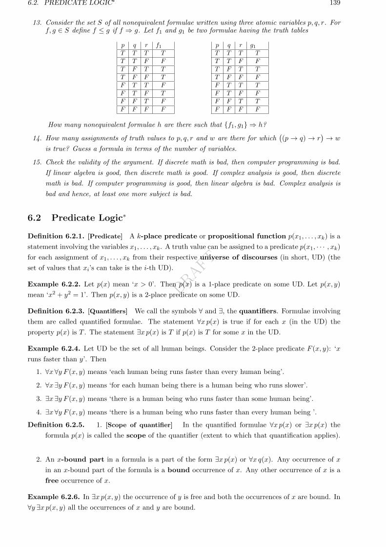
DRAFT

6.2. PREDICATE LOGIC∗ 139

13. Consider the set S of all nonequivalent formulae written using three atomic variables p, q, r. Forf, g ∈ S define f ≤ g if f ⇒ g. Let f1 and g1 be two formulae having the truth tables

p q r f1T T T TT T F FT F T TT F F TF T T FF T F TF F T FF F F F

p q r g1T T T TT T F FT F T TT F F FF T T TF T F FF F T TF F F F

How many nonequivalent formulae h are there such that f1, g1 ⇒ h?

14. How many assignments of truth values to p, q, r and w are there for which((p→ q)→ r

)→ w

is true? Guess a formula in terms of the number of variables.

15. Check the validity of the argument. If discrete math is bad, then computer programming is bad.

If linear algebra is good, then discrete math is good. If complex analysis is good, then discrete

math is bad. If computer programming is good, then linear algebra is bad. Complex analysis is

bad and hence, at least one more subject is bad.

6.2 Predicate Logic∗

Definition 6.2.1. [Predicate] A k-place predicate or propositional function p(x1, . . . , xk) is a

statement involving the variables x1, . . . , xk. A truth value can be assigned to a predicate p(x1, · · · , xk)for each assignment of x1, . . . , xk from their respective universe of discourses (in short, UD) (the

set of values that xi’s can take is the i-th UD).

Example 6.2.2. Let p(x) mean ‘x > 0’. Then p(x) is a 1-place predicate on some UD. Let p(x, y)

mean ‘x2 + y2 = 1’. Then p(x, y) is a 2-place predicate on some UD.

Definition 6.2.3. [Quantifiers] We call the symbols ∀ and ∃, the quantifiers. Formulae involving

them are called quantified formulae. The statement ∀x p(x) is true if for each x (in the UD) the

property p(x) is T . The statement ∃x p(x) is T if p(x) is T for some x in the UD.

Example 6.2.4. Let UD be the set of all human beings. Consider the 2-place predicate F (x, y): ‘x

runs faster than y’. Then

1. ∀x ∀y F (x, y) means ‘each human being runs faster than every human being’.

2. ∀x ∃y F (x, y) means ‘for each human being there is a human being who runs slower’.

3. ∃x ∃y F (x, y) means ‘there is a human being who runs faster than some human being’.

4. ∃x ∀y F (x, y) means ‘there is a human being who runs faster than every human being ’.

Definition 6.2.5. 1. [Scope of quantifier] In the quantified formulae ∀x p(x) or ∃x p(x) the

formula p(x) is called the scope of the quantifier (extent to which that quantification applies).

2. An x-bound part in a formula is a part of the form ∃x p(x) or ∀x q(x). Any occurrence of x

in an x-bound part of the formula is a bound occurrence of x. Any other occurrence of x is a

free occurrence of x.

Example 6.2.6. In ∃x p(x, y) the occurrence of y is free and both the occurrences of x are bound. In

∀y ∃x p(x, y) all the occurrences of x and y are bound.

DRAFT


Definition 6.2.7. 1. A quantified formulae is well formed if it is created using the following rules.

(a) Any atomic formula (of the form P , P (x, y), P (x, b, y)) is a wff.

(b) If A and B are wffs, then A ∨B, A ∧B, A→ B, A↔ B, and ¬A are wffs.

(c) If A is a wff and x is any variable, then ∀xA and ∃xA are wffs.

2. Let f be a formula. An interpretation (for f) means the process of specifying the UD, spec-

ifications of the predicates, and assigning values to the free variables from the UD. By an

interpretation of f , we mean the formula f under a given interpretation.

Example 6.2.8. Consider the wff ∀x p(x, y).

1. Take N as UD. Let p(x, y) specify ‘x > y’. Let us assign 1 to the free variable y. Then, we get

the interpretation ‘each natural number is greater than 1’ which has the truth value F .

2. Take N as UD. Let p(x, y) mean ‘x + y is an integer’, and take y = 2. Then, we get an

interpretation ‘when we add 2 to each natural number we get an integer’ which has a truth value

T .

Discussion 6.2.9. [Translation] We expect to see that ‘our developments on logic’ help us in drawing

appropriate conclusions. In order to do that, we must know how to translate an ‘English statement’

into a ‘formal logical statement’ that involves no English words. We may have to introduce appropriate

variables and required predicates. We may have to specify the UD, but normally we use the most

general UD.

Example 6.2.10. 1. Translate: ‘each person in this class room is either a BTech student or an

MSc student’.

A: Does the statement guarantee that there is a person in the room?

No. All it says is, if there is a person, then it has certain properties. Let P (x) mean ‘x is a

person in this class room’; B(x) mean ‘x is a BTech student’; and M(x) mean ‘x is an MSc

student’. Then, the formal expression is ∀x(P (x)→

(B(x) ∨M(x)

)).

2. Translate: ‘there is a student in this class room who speaks Hindi or English’.

A: Does the statement guarantee that there is a student in the room?

Yes. Let S(x) mean ‘x is a student in this class room’; H(x) mean ‘x speaks Hindi’; and E(x)

mean ‘x speaks English’. Then, the formal expression is ∃x(S(x) ∧ (H(x) ∨ E(x))

).

Note that ∃x(S(x)→ (H(x) ∨ E(x))

)is not the correct expression. Why?

Remember

∃x (S(x)→ T (x)) never asserts S(x) BUT ∃x(S(x) ∧ T (x)) asserts both S(x) and T (x).

Practice 6.2.11. Translate into formal logic.

1. Every natural number is either the square of a natural number or it’s square root is irrational.

2. For every real number x there is a real number y such that x+ y = 0.

3. A subset S ⊆ Rn is called compact, if ‘—write the formal statement here—’.

4. A function f : R→ R is called continuous at a point a, if ‘—write the formal statement here—’.

5. A function f : R→ R is called continuous, if ‘—write the formal statement here—’.

6. A function f : R→ R is called uniformly continuous, if ‘—write the formal statement here—’.

DRAFT


7. A subset S ⊆ Rn is called connected, if ‘—write the formal statement here—’.

8. A set S is called a group, if ‘—write the formal statement here—’.

9. A subset S ⊆ Rn is called a subspace, if ‘—write the formal statement here—’.

10. A function f : S → T is called a bijection, if ‘—write the formal statement here—’.

11. A function f : Rn → Rk is called a linear transformation, if ‘—write the formal statement

here—’.

12. A function f : (S, ) → (T,+) is called a group isomorphism, if ‘—write the formal statement

here—’.

13. A function f : V → W is called a vector space isomorphism, if ‘— write the formal statement

here—’.

Definition 6.2.12. A quantified formula is called valid if every interpretation of it has truth value

T . Two quantified formulae A and B are called equivalent (A ≡ B) if A↔ B is valid.

Example 6.2.13. 1. ∀xP (x) ∨ ∃x¬P (x) is valid.

2. Is ∃x ∃y p(x, y) ≡ ∃y ∃x p(x, y)?

A: Yes. Denote ∃x ∃y p(x, y) by L and ∃y ∃x p(x, y) by R. Suppose that L → R is F . This

means, we have an interpretation in which L is T and R is F . As R is F , we see that p(x, y)

is F , for each x, y in the UD. In that case, L is F , a contradiction. So, L → R is T . Similarly,

R→ L is T .

3. ∀x ∀y p(x, y) ≡ ∀y ∀x p(x, y). !!

4. ∃x ∀y p(x, y) 6≡ ∀y ∃x p(x, y). To see this take p(x, y): x > y.

Did you notice?

Two quantified formulae A and B are equivalent if and only if their interpretations under ‘the

same UD, the same specification of predicates, and the same values to the free variables’ have

the same truth value.

5. Is ∀x(r(x)→ ∃y

(r(y) ∧ p(x, y)

))≡ ∀x∃y

(r(x)→

(r(y) ∧ p(x, y)

))?

A: We want to know if

∀x(r(x)→ ∃y

(r(y) ∧ p(x, y)

))↔ ∀x∃y

(r(x)→

(r(y) ∧ p(x, y)

))is valid. Let us see whether

∀x(r(x)→ ∃y

(r(y) ∧ p(x, y)

))→ ∀x∃y

(r(x)→

(r(y) ∧ p(x, y)

))is valid. Suppose that this is invalid. So there is an interpretation such that Right hand side

is F and Left hand side is T. As Right hand side is F, we see that ∃x, say x0, for which

∃y(r(x)→

(r(y)∧p(x, y)

))is F. That is, ∀y the formula r(x0)→

(r(y)∧p(x0, y)

)is F. That is,

r(x0) is T and for each y we see that r(y)∧p(x0, y) is F. That is, r(x0) is T and ∃y(r(y)∧p(x0, y))

is F. That is, the formula r(x0)→ ∃y(r(y)∧p(x0, y)) is F. That is, ∀x(r(x)→ ∃y

(r(y)∧p(x, y)

))is F, a contradiction. The other part is an exercise.

Alternate. Take A := r(x)→ ∃y(r(y) ∧ p(x, y)

)and B := ∃y

(r(x)→

(r(y) ∧ p(x, y)

)).

DRAFT


Consider an x0 in the UD. If r(x0) is F, Then A and B both have value T. If r(x0) is T. Then

notice that r(x0)→ ∃y(r(y) ∧ p(x0, y)

)and ∃y

(r(x0)→

(r(y) ∧ p(x0, y)

))have the same truth

value.

Thus A ≡ B. Hence ∀xA ≡ ∀xB.

6. Any student who appears in the exam and gets a score below 30, gets an F grade. Mr x0 is a

student who has not written the exam. Therefore, x0 should get an F grade. Do you agree?

A: Let S(x) mean ‘x is a student’, E(x) mean ‘x writes the exam’, B(x) mean ‘x gets a score

below 30’, and F (x) mean ‘x gets F grade’.

We want to see whether∀x[S(x) ∧ E(x) ∧B(x)→ F (x)], S(x0) ∧ ¬E(x0)

⇒ F (x0)?

Take the following interpretation: S(x) is ‘x is a positive real number’, E(x) is ‘x is a rational

number’, B(x) is ‘x is an integer’, F (x) is ‘x is a natural number’, and x0 =√

2.

In this interpretation, statements in the premise mean ‘every positive integer is a natural number’

and ‘√

2 is a positive real number which is not rational’. They both are true. Whereas the

conclusion means ‘√

2 is a natural number’ which is false. So, the argument is incorrect.

7. Translate the following into formal statements.

‘All scientists are human beings. Therefore, all children of scientists are children of human

beings.’

A: Let Sx : ‘x is a scientist’; Hx : ‘x is a human being’ and Cxy : x is a child of y.

Let the hypothesis be ∀x(Sx → Hx). Then, the possible translations of the conclusion are the

following.

(a) ∀x(∃y(Sy ∧ Cxy)→ ∃z(Hz ∧ Cxz)). It means ‘for each x, if x has a scientist father, then

x has a human father’.

(b) ∀x[∀y(Sy ∧ Cxy)→ ∀z(Hz ∧ Cxz)]. This is wrong, as the statement means ‘for all x, if x

is a common child of all scientists, then x is a common child of all human beings’.

(c) ∀x(Sx→ ∀y(Cyx→ ∃z(Hz ∧ Cyz))). This means ‘for each x, if x is a scientist, then each

child of x has a human father’.

(d) ∀x∀y(Sx ∧Cyx)→ ∀x∀y(Hx ∧Cxy). What? This means ‘if each x is a scientist and each

y is a child of x (including x it self!), then each x is a human being and each y is a child of

x’.

Exercise 6.2.14. 1. Write a formal definition of limx→a

f(x) 6= l.

2. Is ∃x [p(x) ∧ q(x)]→ ∃x p(x) ∧ ∃x q(x) valid? Is it’s converse valid?

3. [common ones] If r does not involve x, then establish the following assertions.

(a) ¬∀x p(x) ≡ ∃x¬p(x); ¬∃x p(x) ≡ ∀x¬p(x)

(b) ∃x(p(x) ∨ q(x)

)≡ ∃x p(x) ∨ ∃x q(x); ∃x

(p(x) ∧ q(x)

)⇒ ∃x p(x) ∧ ∃x q(x).

(c) ∀x(p(x) ∧ q(x)

)≡ ∀x p(x) ∧ ∀x q(x); ∀x

(p(x) ∨ q(x)

)⇐ ∀x p(x) ∨ ∀x q(x).

(d) ∀x(r ∨ q(x)

)≡ r ∨ ∀x q(x); ∀x

(r → q(x)

)≡ r → ∀x q(x)

(e) ∃x(r ∧ q(x)

)≡ r ∧ ∃x q(x); ∃x

(r → q(x)

)≡ r → ∃x q(x).

(f) ∀x p(x)→ r ≡ ∃x(p(x)→ r

); ∃x p(x)→ r ≡ ∀x

(p(x)→ r

).

4. Translate and check for validity of the following arguments.

(a) Recall that the decimal representation of a rational number either terminates or begins

to repeat the same finite sequence of digits, whereas that of an irrational number neither

DRAFT


terminates nor repeats. The square root of a natural number either has a decimal represen-

tation which is terminating or has a decimal representation which is non-terminating and

non-repeating. The square root of all natural numbers which are squares have terminating

decimal representation. Therefore, the square root of a natural number which is not a square

is an irrational number.

(b) For any two algebraic numbers a and b, a 6= 0, 1 and b irrational, we have that ab is

transcendental. The number i (imaginary unit) is irrational and algebraic. The number i

is not equal to 0 or 1. Therefore, the number ii is transcendental.

5. (a) Give an interpretation to show that ∀x(r(x)→ ∃y

(r(y) ∧ p(x, y)

))is not valid.

(b) Give an interpretation to show the incorrectness of ∀x(p(x) → q(x)

)⇒ ∃x

(¬p(x) →

¬q(x)).

6. Write a formal statement taking UD:= all students in all IIT’s in India, for the following.

‘For each student in IITG there is a student in IITG with more CPI.’

7. Let UD= R, p(x): x is an integer, and q(x): x is a rational number. Translate the following

statements into English.

(a) ∀x(p(x)→ q(x)

)(b) ∃x

(¬p(x) ∧ q(x)

)(c) ∀x

(p(x) ∧ (x > 2)

)→ ∀x

(q(x) ∧ (x < 2)

)(d) ∃ε > 0

(∀δ > 0(0 < |x− a| < δ → |f(x)− l| < ε)

)8. Take the most general UD. Check whether the following conclusion is valid or not.

Each student writes the exam using blue ink or black ink. A student who writes the exam using

black ink and does not write his/her roll number gets an F grade. A student who writes the exam

using blue ink and does not have his/her ID card gets an F grade. A student who has his/her

ID card has written the exam with black ink. Therefore, a student who passes the exam must

have written his roll number.

DRAFT


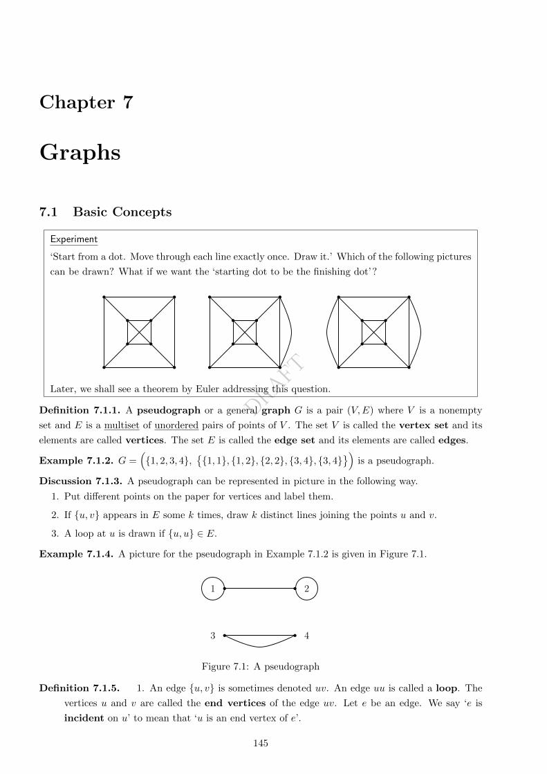
DRAFT

Chapter 7

Graphs

7.1 Basic Concepts

Experiment

‘Start from a dot. Move through each line exactly once. Draw it.’ Which of the following pictures

can be drawn? What if we want the ‘starting dot to be the finishing dot’?

Later, we shall see a theorem by Euler addressing this question.

Definition 7.1.1. A pseudograph or a general graph G is a pair (V,E) where V is a nonempty

set and E is a multiset of unordered pairs of points of V . The set V is called the vertex set and its

elements are called vertices. The set E is called the edge set and its elements are called edges.

Example 7.1.2. G =(1, 2, 3, 4,

1, 1, 1, 2, 2, 2, 3, 4, 3, 4

)is a pseudograph.

Discussion 7.1.3. A pseudograph can be represented in picture in the following way.

1. Put different points on the paper for vertices and label them.

2. If u, v appears in E some k times, draw k distinct lines joining the points u and v.

3. A loop at u is drawn if u, u ∈ E.

Example 7.1.4. A picture for the pseudograph in Example 7.1.2 is given in Figure 7.1.

1 2

3 4

Figure 7.1: A pseudograph

Definition 7.1.5. 1. An edge u, v is sometimes denoted uv. An edge uu is called a loop. The

vertices u and v are called the end vertices of the edge uv. Let e be an edge. We say ‘e is

incident on u’ to mean that ‘u is an end vertex of e’.

145

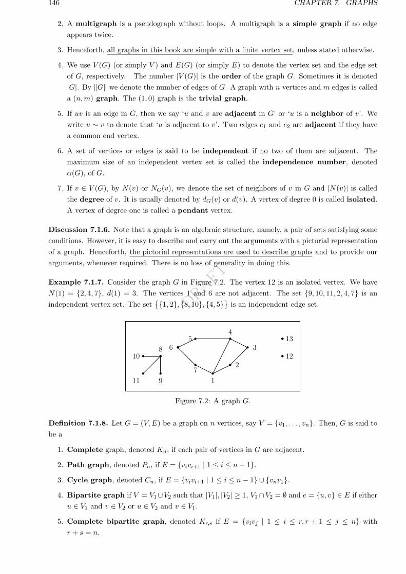
DRAFT

146 CHAPTER 7. GRAPHS

2. A multigraph is a pseudograph without loops. A multigraph is a simple graph if no edge

appears twice.

3. Henceforth, all graphs in this book are simple with a finite vertex set, unless stated otherwise.

4. We use V (G) (or simply V ) and E(G) (or simply E) to denote the vertex set and the edge set

of G, respectively. The number |V (G)| is the order of the graph G. Sometimes it is denoted

|G|. By ‖G‖ we denote the number of edges of G. A graph with n vertices and m edges is called

a (n,m) graph. The (1, 0) graph is the trivial graph.

5. If uv is an edge in G, then we say ‘u and v are adjacent in G’ or ‘u is a neighbor of v’. We

write u ∼ v to denote that ‘u is adjacent to v’. Two edges e1 and e2 are adjacent if they have

a common end vertex.

6. A set of vertices or edges is said to be independent if no two of them are adjacent. The

maximum size of an independent vertex set is called the independence number, denoted

α(G), of G.

7. If v ∈ V (G), by N(v) or NG(v), we denote the set of neighbors of v in G and |N(v)| is called

the degree of v. It is usually denoted by dG(v) or d(v). A vertex of degree 0 is called isolated.

A vertex of degree one is called a pendant vertex.

Discussion 7.1.6. Note that a graph is an algebraic structure, namely, a pair of sets satisfying some

conditions. However, it is easy to describe and carry out the arguments with a pictorial representation

of a graph. Henceforth, the pictorial representations are used to describe graphs and to provide our

arguments, whenever required. There is no loss of generality in doing this.

Example 7.1.7. Consider the graph G in Figure 7.2. The vertex 12 is an isolated vertex. We have

N(1) = 2, 4, 7, d(1) = 3. The vertices 1 and 6 are not adjacent. The set 9, 10, 11, 2, 4, 7 is an

independent vertex set. The set1, 2, 8, 10, 4, 5

is an independent edge set.

11

810

9 1

2

3

45

6

7

12

13

Figure 7.2: A graph G.

Definition 7.1.8. Let G = (V,E) be a graph on n vertices, say V = v1, . . . , vn. Then, G is said to

be a

1. Complete graph, denoted Kn, if each pair of vertices in G are adjacent.

2. Path graph, denoted Pn, if E = vivi+1 | 1 ≤ i ≤ n− 1.

3. Cycle graph, denoted Cn, if E = vivi+1 | 1 ≤ i ≤ n− 1 ∪ vnv1.

4. Bipartite graph if V = V1∪V2 such that |V1|, |V2| ≥ 1, V1 ∩V2 = ∅ and e = u, v ∈ E if either

u ∈ V1 and v ∈ V2 or u ∈ V2 and v ∈ V1.

5. Complete bipartite graph, denoted Kr,s if E = vivj | 1 ≤ i ≤ r, r + 1 ≤ j ≤ n with

r + s = n.

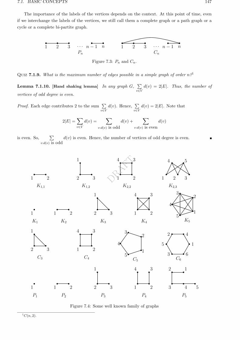
DRAFT

7.1. BASIC CONCEPTS 147

The importance of the labels of the vertices depends on the context. At this point of time, even

if we interchange the labels of the vertices, we still call them a complete graph or a path graph or a

cycle or a complete bi-partite graph.

1 2 3 n − 1 n· · ·Pn

1 2 3 n − 1 n· · ·Cn

1 2 3 n − 1 n· · ·Pn

1 2 3 n − 1 n· · ·Cn

Figure 7.3: Pn and Cn.

Quiz 7.1.9. What is the maximum number of edges possible in a simple graph of order n?1

Lemma 7.1.10. [Hand shaking lemma] In any graph G,∑v∈V

d(v) = 2|E|. Thus, the number of

vertices of odd degree is even.

Proof. Each edge contributes 2 to the sum∑v∈V

d(v). Hence,∑v∈V

d(v) = 2|E|. Note that

2|E| =∑v∈V

d(v) =∑

v:d(v) is odd

d(v) +∑

v:d(v) is even

d(v)

is even. So,∑

v:d(v) is oddd(v) is even. Hence, the number of vertices of odd degree is even.

1

P1

1 2

P2

2

1

3

P3

1

4

2

3

P4

3

2

4

1

5

P5

1

K1

1 2

K2

2

1

3

K3

1

4

2

3

K4

1

23

4

5K5

2

1

3

C3

1

4

2

3

C4

1

23

4

5C5

15

42

63C6

1 2

K1,1

2

1

3

K1,2

1

4

2

3

K2,2

1 2 3

4 5

K2,3

1

Figure 7.4: Some well known family of graphs

1C(n, 2).

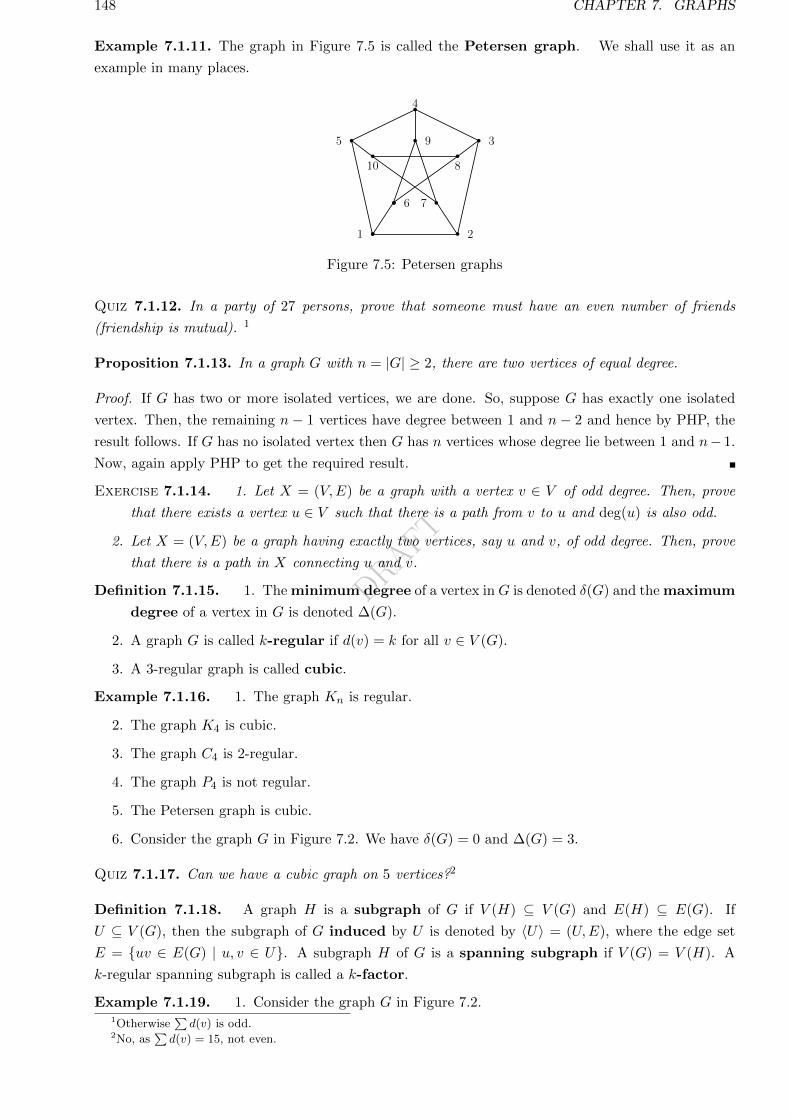
DRAFT


Example 7.1.11. The graph in Figure 7.5 is called the Petersen graph. We shall use it as an

example in many places.

1 2

3

4

5

6 7

8

9

10

Figure 7.5: Petersen graphs

Quiz 7.1.12. In a party of 27 persons, prove that someone must have an even number of friends

(friendship is mutual). 1

Proposition 7.1.13. In a graph G with n = |G| ≥ 2, there are two vertices of equal degree.

Proof. If G has two or more isolated vertices, we are done. So, suppose G has exactly one isolated

vertex. Then, the remaining n− 1 vertices have degree between 1 and n− 2 and hence by PHP, the

result follows. If G has no isolated vertex then G has n vertices whose degree lie between 1 and n− 1.

Now, again apply PHP to get the required result.

Exercise 7.1.14. 1. Let X = (V,E) be a graph with a vertex v ∈ V of odd degree. Then, prove

that there exists a vertex u ∈ V such that there is a path from v to u and deg(u) is also odd.

2. Let X = (V,E) be a graph having exactly two vertices, say u and v, of odd degree. Then, prove

that there is a path in X connecting u and v.

Definition 7.1.15. 1. The minimum degree of a vertex in G is denoted δ(G) and the maximum

degree of a vertex in G is denoted ∆(G).

2. A graph G is called k-regular if d(v) = k for all v ∈ V (G).

3. A 3-regular graph is called cubic.

Example 7.1.16. 1. The graph Kn is regular.

2. The graph K4 is cubic.

3. The graph C4 is 2-regular.

4. The graph P4 is not regular.

5. The Petersen graph is cubic.

6. Consider the graph G in Figure 7.2. We have δ(G) = 0 and ∆(G) = 3.

Quiz 7.1.17. Can we have a cubic graph on 5 vertices?2

Definition 7.1.18. A graph H is a subgraph of G if V (H) ⊆ V (G) and E(H) ⊆ E(G). If

U ⊆ V (G), then the subgraph of G induced by U is denoted by 〈U〉 = (U,E), where the edge set

E = uv ∈ E(G) | u, v ∈ U. A subgraph H of G is a spanning subgraph if V (G) = V (H). A

k-regular spanning subgraph is called a k-factor.

Example 7.1.19. 1. Consider the graph G in Figure 7.2.1Otherwise

∑d(v) is odd.

2No, as∑d(v) = 15, not even.

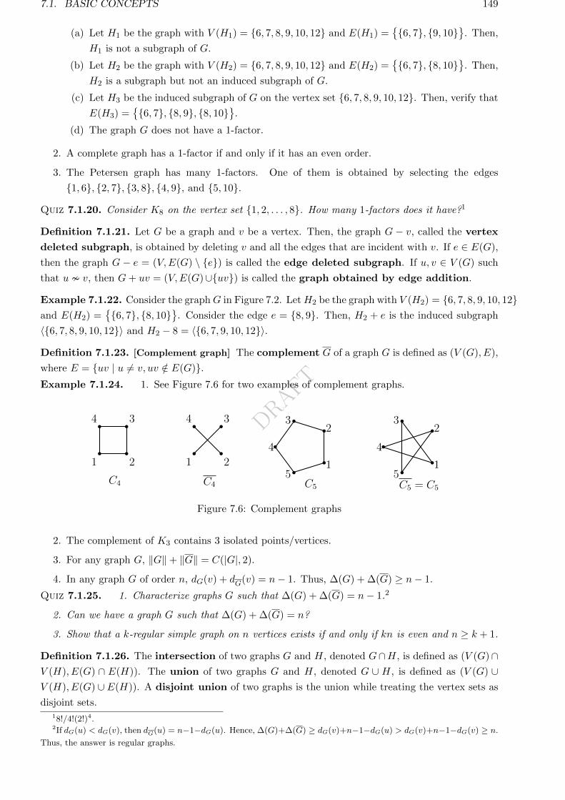
DRAFT

7.1. BASIC CONCEPTS 149

(a) Let H1 be the graph with V (H1) = 6, 7, 8, 9, 10, 12 and E(H1) =6, 7, 9, 10

. Then,

H1 is not a subgraph of G.

(b) Let H2 be the graph with V (H2) = 6, 7, 8, 9, 10, 12 and E(H2) =6, 7, 8, 10

. Then,

H2 is a subgraph but not an induced subgraph of G.

(c) Let H3 be the induced subgraph of G on the vertex set 6, 7, 8, 9, 10, 12. Then, verify that

E(H3) =6, 7, 8, 9, 8, 10

.

(d) The graph G does not have a 1-factor.

2. A complete graph has a 1-factor if and only if it has an even order.

3. The Petersen graph has many 1-factors. One of them is obtained by selecting the edges

1, 6, 2, 7, 3, 8, 4, 9, and 5, 10.

Quiz 7.1.20. Consider K8 on the vertex set 1, 2, . . . , 8. How many 1-factors does it have?1

Definition 7.1.21. Let G be a graph and v be a vertex. Then, the graph G − v, called the vertex

deleted subgraph, is obtained by deleting v and all the edges that are incident with v. If e ∈ E(G),

then the graph G − e = (V,E(G) \ e) is called the edge deleted subgraph. If u, v ∈ V (G) such

that u v, then G+ uv = (V,E(G)∪uv) is called the graph obtained by edge addition.

Example 7.1.22. Consider the graphG in Figure 7.2. LetH2 be the graph with V (H2) = 6, 7, 8, 9, 10, 12and E(H2) =

6, 7, 8, 10

. Consider the edge e = 8, 9. Then, H2 + e is the induced subgraph

〈6, 7, 8, 9, 10, 12〉 and H2 − 8 = 〈6, 7, 9, 10, 12〉.

Definition 7.1.23. [Complement graph] The complement G of a graph G is defined as (V (G), E),

where E = uv | u 6= v, uv /∈ E(G).Example 7.1.24. 1. See Figure 7.6 for two examples of complement graphs.

1

4

2

3

C4

1

4

2

3

C4

1

23

4

5C5

1

23

4

5C5 = C5

1

Figure 7.6: Complement graphs

2. The complement of K3 contains 3 isolated points/vertices.

3. For any graph G, ‖G‖+ ‖G‖ = C(|G|, 2).

4. In any graph G of order n, dG(v) + dG(v) = n− 1. Thus, ∆(G) + ∆(G) ≥ n− 1.

Quiz 7.1.25. 1. Characterize graphs G such that ∆(G) + ∆(G) = n− 1.2

2. Can we have a graph G such that ∆(G) + ∆(G) = n?

3. Show that a k-regular simple graph on n vertices exists if and only if kn is even and n ≥ k + 1.

Definition 7.1.26. The intersection of two graphs G and H, denoted G∩H, is defined as (V (G)∩V (H), E(G) ∩ E(H)). The union of two graphs G and H, denoted G ∪ H, is defined as (V (G) ∪V (H), E(G) ∪ E(H)). A disjoint union of two graphs is the union while treating the vertex sets as

disjoint sets.18!/4!(2!)4.2If dG(u) < dG(v), then dG(u) = n−1−dG(u). Hence, ∆(G)+∆(G) ≥ dG(v)+n−1−dG(u) > dG(v)+n−1−dG(v) ≥ n.

Thus, the answer is regular graphs.

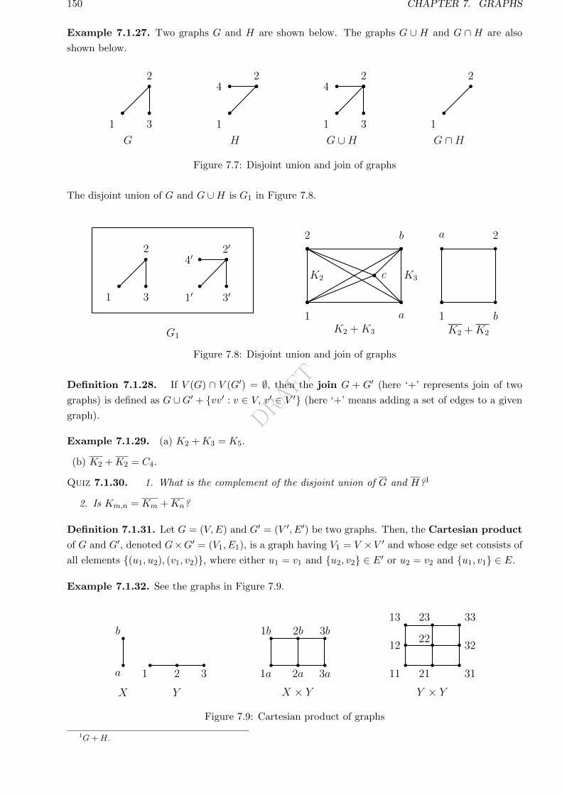
DRAFT


Example 7.1.27. Two graphs G and H are shown below. The graphs G ∪ H and G ∩ H are also

shown below.

1

2

3

G

1

24

H

1

24

3

G ∪ H

1

2

G ∩ H

Figure 7.7: Disjoint union and join of graphs

The disjoint union of G and G ∪H is G1 in Figure 7.8.

1

2

3 1′

2′

4′

3′

G1

1

2

a

b

cK2 K3

K2 + K3

1

a

b

2

K2 + K2

1

Figure 7.8: Disjoint union and join of graphs

Definition 7.1.28. If V (G) ∩ V (G′) = ∅, then the join G + G′ (here ‘+’ represents join of two

graphs) is defined as G ∪G′ + vv′ : v ∈ V, v′ ∈ V ′ (here ‘+’ means adding a set of edges to a given

graph).

Example 7.1.29. (a) K2 +K3 = K5.

(b) K2 +K2 = C4.

Quiz 7.1.30. 1. What is the complement of the disjoint union of G and H?1

2. Is Km,n = Km +Kn?

Definition 7.1.31. Let G = (V,E) and G′ = (V ′, E′) be two graphs. Then, the Cartesian product

of G and G′, denoted G×G′ = (V1, E1), is a graph having V1 = V ×V ′ and whose edge set consists of

all elements (u1, u2), (v1, v2), where either u1 = v1 and u2, v2 ∈ E′ or u2 = v2 and u1, v1 ∈ E.

Example 7.1.32. See the graphs in Figure 7.9.

a

b

X

1 2 3

Y

1a 2a 3a

1b 2b 3b

X × Y

11 21 31

1222

32

13 23 33

Y × Y

1

Figure 7.9: Cartesian product of graphs

1G+H.

DRAFT

7.2. CONNECTEDNESS 151

7.2 Connectedness

Definition 7.2.1. An u-v walk in G is a finite sequence of vertices [u = v1, v2, · · · , vk = v] such

that vivi+1 ∈ E, for all i = 1, · · · , k − 1. The length of a walk is the number of edges on it. A

walk is called a trail if edges on the walk are not repeated. A v-u walk is a called a path if the

vertices involved are all distinct, except that v and u may be the same. A path can have length 0.

A walk (trail, path) is called closed if u = v. A closed path is called a cycle/circuit. Thus, in a

simple graph a cycle has length at least 3. A cycle (walk, path) of length k is also written as a k-cycle

(k-walk, k-path). If P is an u-v path with u 6= v, then we sometimes call u and v as the end vertices

of P and the remaining vertices on P as the internal vertices.

Example 7.2.2.

(a) Take G = K5 with vertex set 1, 2, 3, 4, 5.• Then, [1, 2, 3, 2, 1, 2, 5, 4, 3] is a 8-walk in G and [1, 2, 2, 1] is not a walk.

• The walk [1, 2, 3, 4, 5, 2, 4, 1] is a closed trail.

• The walk [1, 2, 3, 5, 4, 1] is a closed path, that is, it is a 5-cycle.

• The maximum length of a cycle in G is 5 and the minimum length of a cycle in G is 3.

• There are 10 = C(5, 3) many 3-cycles in G.

• Verify that the number of 4-cycles in G is not C(5, 4). Can it be 3× C(5, 4)?

(b) Let G be the Petersen graph.

• There is a 9-cycle in G, namely, [6, 8, 10, 5, 4, 3, 2, 7, 9, 6].

• There are no 10-cycles in G. We shall see this when we discuss the Eulerian graphs.

Proposition 7.2.3 (Technique). Let G be a graph and u, v ∈ V (G), u 6= v. Let W = [u = u1, . . . , uk =

v] be a walk. Then, W contains an u-v-path.

Proof. If no vertex on W repeats, then W is itself a path. So, let ui = uj for some i < j. Now,

consider the walk W1 = [u1, . . . , ui−1, uj , uj+1, . . . uk]. This is also an u-v walk but of shorter length.

Thus, using induction on the length of the walk, the desired result follows.

Definition 7.2.4. The distance d(u, v) between two vertices u and v in G is the shortest length

of an u-v path in G. If no such path exists, the distance is taken to be ∞. The greatest distance

between any two vertices in a graph G is called the diameter of G. We shall use diam(G) to denote

the diameter of G. Let distv = maxu∈G

d(v, u). The radius is the minv∈G

distv and the center consists of

all vertices v for which distv is the radius. The girth, denoted g(G), of a graph G is the minimum

length of a cycle contained in G. If G has no cycle, then we put g(G) =∞.

Example 7.2.5. Let G be the Petersen graph. It has diameter 2. The radius is 2. Each vertex is in

the center. Its girth is 5.

Practice 7.2.6. Determine the diameter, radius, center and girth of the following graphs: Pn, Cn,

Kn and Kn,m.

Exercise 7.2.7. Let G be a graph. Then, show that the distance function d(u, v) is a metric on V (G).

That is, it satisfies

1. d(u, v) ≥ 0 for all u, v ∈ V (G) and d(u, v) = 0 if and only if u = v,

2. d(u, v) = d(v, u) for all u, v ∈ V (G) and

3. d(u, v) ≤ d(u,w) + d(w, u) for all u, v, w ∈ V (G).

DRAFT


Proposition 7.2.8 (Technique). Let G be a graph with ‖G‖ ≥ 1 and d(v) ≥ 2, for each vertex except

one, say v1. Then, G has a cycle.

Proof. Consider a longest path [v1, . . . , vk] in G (as V (G) is finite, such a path exists). As d(vk) ≥ 2,

it must be adjacent to some vertex from v2, . . . , vk−2, otherwise, we can extend it to a longer path.

Let i ≥ 2 be the smallest such that vi is adjacent to vk. Then, [vi, vi+1, . . . , vk, vi] is a cycle.

Proposition 7.2.9 (Technique). Let P and Q be two different u-v paths in G. Then, P ∪Q contains

a cycle.

Proof. Imagine a signal was sent from u to v via P and was returned back from v to u via Q. Call an

edge ‘dead’ if signal has passed through it twice. Notice that each vertex receives the signal as many

times as it sends the signal.

Is E(P ) = E(Q)? No, otherwise both P and Q are the same paths.

So, there are some ‘alive’ edges. Get an alive edge −−→v1v2. There must be an alive edge −−→v2v3.1 Simi-

larly get −−→v3v4 and so on. Stop at the first instance of repetition of a vertex: [v1, v2, · · · , vi, vi+1 · · · , vj =

vi]. Then, [vi, vi+1 · · · , vj = vi] is a cycle.

Alternate. Consider the graph H =(V (P ) ∪ V (Q), E(P )∆E(Q)

), where ∆ is the symmetric

difference. Notice that E(H) 6= ∅, otherwise P = Q. As the degree of each vertex in the multigraph

P ∪ Q is even and H is obtained after deleting pairs of multiple edges, each vertex in H has even

degree. Hence, by Proposition 7.2.8, H has a cycle.

Proposition 7.2.10. Every graph G containing a cycle satisfies g(G) ≤ 2 diam(G) + 1.

Proof. Let C = [v1, v2, . . . , vk, v1] be the shortest cycle and diam(G) = r. If k ≥ 2r + 2, then consider

the path P = [v1, v2, . . . , vr+2]. Since the length of P is r + 1 and diam(G) = r, there is a vr+2-v1

path R of length at most r. Note that P and R are different v1-vr+2 paths. By Proposition 7.2.9, the

closed walk P ∪R of length at most 2r+ 1 contains a cycle. Hence, the length of this cycle is at most

2r + 1, a contradiction to C having the smallest length k ≥ 2r + 2.

Definition 7.2.11. Let C = [v1, . . . , vk = v1] be a cycle. An edge vivj is called a chord of C if it is

not an edge of C. A graph is called chordal if each cycle of length at least 4 has a chord. A graph is

acyclic if it has no cycles.

Example 7.2.12. Complete graphs are chordal, so are the acyclic graphs. The Petersen graph is not

chordal.

Quiz 7.2.13. 1. How many acyclic graphs are there on the vertex set 1, 2, 3?2

2. How many chordal graphs are there on the vertex set 1, 2, 3, 4?3

Definition 7.2.14. 1. A graph G is said to be maximal with respect to a property P if G has

property P and no proper supergraph of G has the property P . We similarly define the term

minimal.

Notice!

The class of all graphs with that property is the POSET here. So, the maximality and the

minimality are defined naturally.

1Otherwise, v2 is incident to just one alive edge and some dead edges. This means v2 has received more signal than

it has sent.27: 3 edges can be put in 23 ways. One of them is a cycle.361: 6 edges can be put in 26 ways. There are three 4-cycles.

DRAFT

7.2. CONNECTEDNESS 153

2. A complete subgraph of G is called a clique. The maximum order of a clique is called the clique

number of G. It is denoted ω(G).

3. A graph G is called connected if there is an u-v path, for each u, v ∈ V (G).

4. A graph which is not connected is called disconnected. If G is a disconnected graph, then a

maximal connected subgraph is called a component or sometimes a connected component.

Example 7.2.15. Consider the graph G shown in Figure 7.2. Then,

1. some cliques in G are 〈8, 10〉, 〈2〉. The first is a maximal cliques. Notice that every vertex

is a clique. Similarly each edge is a clique. Here ω(G) = 2.

2. the graph G is not connected. It has four connected components, namely, 〈8, 9, 10, 11〉,〈1, 2, 3, 4, 5, 6, 7〉, 〈12〉 and 〈13〉.

Quiz 7.2.16. What is ω(G) for the Petersen graph?1

Proposition 7.2.17. If δ(G) ≥ 2, then G has a path of length δ(G) and a cycle of length at least

δ(G) + 1.

Proof. Let [v1, · · · , vk] be a longest path in G. As d(vk) ≥ 2, vk is adjacent to some vertex v 6= vk−1.

If v is not on the path, then we have a path that is longer than [v1, · · · , vk] path. A contradiction.

Let i be the smallest positive integer such that vi is adjacent to vk. Thus,

δ(G) ≤ d(vk) ≤ |vi, vi+1, · · · , vk−1|.

Hence, the cycle C = [vi, vi+1, · · · , vk, vi] has length at least δ(G) + 1 and the length of the path

P = [vi, vi+1, · · · , vk] is at least δ(G).

Definition 7.2.18. The edge density, denoted ε(G), is defined to be the number |E(G)||V (G)| . Observe

that ε(G) is also a graph invariant.

Quiz 7.2.19. 1. When does ‘deletion of a vertex’ reduce edge density?2

2. Is δ(G)2 a lower bound for ε(G)?3

3. Suppose that ε(G) ≥ δ(G). Should we have a vertex v with ε(G) ≥ d(v)?4

Proposition 7.2.20. Let G be a graph with ‖G‖ ≥ 1. Then, G has a subgraph H with δ(H) > ε(H) ≥ε(G).

Proof. If ε(G) < δ(G), then we take H = G. Otherwise, there is a vertex v with ε(G) ≥ d(v). Put

G1 = G− v. Then, it can be easily verified that ε(G1) ≥ ε(G).

If ε(G1) < δ(G1), then we take H = G1. Otherwise, there is a vertex v ∈ G1 with ε(G1) ≥ d(v).

Put G2 = G1 − v. Then, we again have ε(G2) ≥ ε(G1) ≥ ε(G).

Continuing as above, we note that “Initially ε(G) > 0. At the i-th stage, we obtained the subgraph

Gi satisfying |V (Gi)| = |G|−i, ε(Gi) ≥ ε(Gi−1). That is, we have been reducing the number of vertices

and the corresponding edge densities have been non-decreasing.” Hence, this process must stop before

we reach a single vertex, as its edge density is 0.

So, let us assume that the process stops at H. Then, ‘ε(H) < δ(H)’ must be true, or else, the

process would not stop at H and hence the required result follows.

12.2Put H = G− v. Then, ‖H‖ = ε(G)n− d(v), so that ε(H) = ε(G)n−d(v)

n−1= ε(G) + ε(G)−d(v)

n−1. So, we should choose a

vertex v with degree more that ε(G).3Yes.4Yes. Otherwise, we have ε(G) < d(v), for each v. In particular ε(G) < δ(G), a contradiction.

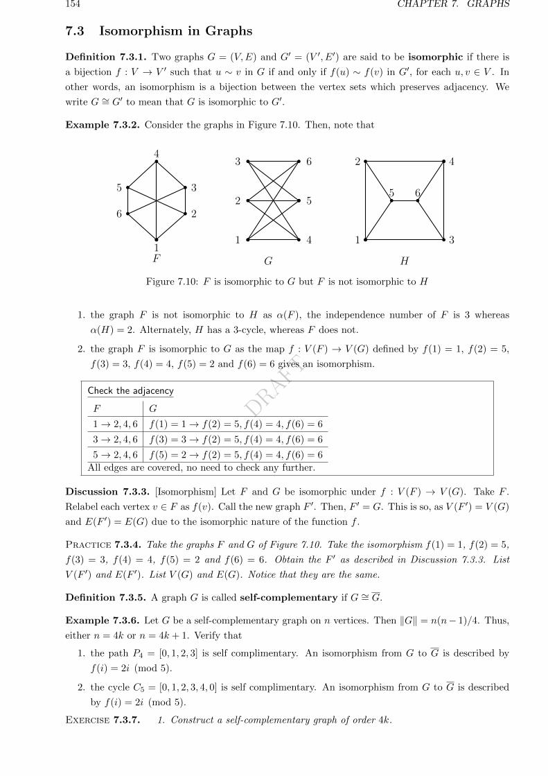
DRAFT


7.3 Isomorphism in Graphs

Definition 7.3.1. Two graphs G = (V,E) and G′ = (V ′, E′) are said to be isomorphic if there is

a bijection f : V → V ′ such that u ∼ v in G if and only if f(u) ∼ f(v) in G′, for each u, v ∈ V . In

other words, an isomorphism is a bijection between the vertex sets which preserves adjacency. We

write G ∼= G′ to mean that G is isomorphic to G′.

Example 7.3.2. Consider the graphs in Figure 7.10. Then, note that

F1

2

3

4

6

5

G

1

2

3

4

5

6

H

1

2

3

4

5 6

Figure 7.10: F is isomorphic to G but F is not isomorphic to H

1. the graph F is not isomorphic to H as α(F ), the independence number of F is 3 whereas

α(H) = 2. Alternately, H has a 3-cycle, whereas F does not.

2. the graph F is isomorphic to G as the map f : V (F ) → V (G) defined by f(1) = 1, f(2) = 5,

f(3) = 3, f(4) = 4, f(5) = 2 and f(6) = 6 gives an isomorphism.

Check the adjacency

F G

1→ 2, 4, 6 f(1) = 1→ f(2) = 5, f(4) = 4, f(6) = 6

3→ 2, 4, 6 f(3) = 3→ f(2) = 5, f(4) = 4, f(6) = 6

5→ 2, 4, 6 f(5) = 2→ f(2) = 5, f(4) = 4, f(6) = 6

All edges are covered, no need to check any further.

Discussion 7.3.3. [Isomorphism] Let F and G be isomorphic under f : V (F ) → V (G). Take F .

Relabel each vertex v ∈ F as f(v). Call the new graph F ′. Then, F ′ = G. This is so, as V (F ′) = V (G)

and E(F ′) = E(G) due to the isomorphic nature of the function f .

Practice 7.3.4. Take the graphs F and G of Figure 7.10. Take the isomorphism f(1) = 1, f(2) = 5,

f(3) = 3, f(4) = 4, f(5) = 2 and f(6) = 6. Obtain the F ′ as described in Discussion 7.3.3. List

V (F ′) and E(F ′). List V (G) and E(G). Notice that they are the same.

Definition 7.3.5. A graph G is called self-complementary if G ∼= G.

Example 7.3.6. Let G be a self-complementary graph on n vertices. Then ‖G‖ = n(n− 1)/4. Thus,

either n = 4k or n = 4k + 1. Verify that

1. the path P4 = [0, 1, 2, 3] is self complimentary. An isomorphism from G to G is described by

f(i) = 2i (mod 5).

2. the cycle C5 = [0, 1, 2, 3, 4, 0] is self complimentary. An isomorphism from G to G is described

by f(i) = 2i (mod 5).

Exercise 7.3.7. 1. Construct a self-complementary graph of order 4k.

DRAFT

7.3. ISOMORPHISM IN GRAPHS 155

2. Construct a self-complementary graph of order 4k + 1.

Definition 7.3.8. A graph invariant is a function which assigns the same value (output) to iso-

morphic graphs.

Example 7.3.9. Observe that some of the graph invariants are: |G|, ‖G‖, ∆(G), δ(G), ω(G), α(G)

and the multiset d(v) : v ∈ V (G).

Exercise 7.3.10. How many graphs are there with vertex set 1, 2, . . . , n? Do you find it easy if we

ask for non-isomorphic graphs (try for n = 4)?

Proposition 7.3.11 (Technique). Let f : G→ H be an isomorphism and v ∈ V (G). Then, G− v ∼=H − f(v).

Proof. Consider the bijection g : V (G− v)→ V (H − f(v)) described by g = fV (G−v).

Definition 7.3.12. An isomorphism of G to G is called an automorphism.

Example 7.3.13. 1. Identity map is always an automorphism on any graph.

2. Any permutation in Sn is an automorphism of Kn.

3. There are only two automorphisms of a path P8. Is it true for Pn, for n ≥ 3?

Proposition 7.3.14. Let G be a graph and let Γ(G) denote the set of all automorphisms of G. Then,

Γ(G) forms a group under composition of functions.

Proof. Let V (G) = 1, 2, . . . , n and σ, µ ∈ Γ(G) be two automorphisms. Then,

ij ∈ E(G)⇔ µ(i)µ(j) ∈ E(G)⇔ (σ µ)(i)(σ µ)(j) ∈ E(G).

Thus, σ µ is an automorphism. Moreover, µ−1, σ−1 are indeed automorphisms.

Example 7.3.15. Determine Γ(C5).

Ans: Consider C5 = [1, . . . , 5, 1]. Note that σ = (2, 3, 4, 5, 1) is an automorphism. Hence,

e, σ, σ2, . . . , σ4 ⊆ Γ(C5) as σ5 = e.

Now, let µ be an automorphism with µ(1) = i. Put τ = σ6−iµ. Then, τ is an automorphism with

τ(1) = 1. If τ(2) = 2, then the adjacency structure implies that τ(j) = j for j = 3, 4, 5. Hence, in this

case, σ6−iµ = e and thus, µ = σi−6 = σi−1.

If τ(2) 6= 2, then τ(2) = 5, τ(3) = 4 and so τ = (2, 5)(3, 4) is the reflection which fixes 1. Let us

denote the permutation (2, 5)(3, 4) by ρ. Then, Γ(C5) is the group generated by σ and ρ and hence

Γ(C5) has 10 elements.

Example 7.3.16. Notice that Γ(C5) has a subgroup Γ1 = e, σ, σ2, σ3, σ4, with σ5 = e, of order

5. Let G be a subgraph of C5 obtained by deleting some (zero allowed) edges. If ‖G‖ = 5, then

|Γ(G)| = 10. If ‖G‖ = 0, then |Γ(G)| = |S5| = 5!. If ‖G‖ = 4, then |Γ(G)| = 2. If ‖G‖ = 3, then

|Γ(G)| = 2 or 4. If ‖G‖ = 2, then |Γ(G)| = 4 or 8. If ‖G‖ = 1, then |Γ(G)| = 2× 3!. Thus, there is no

subgraph of G whose automorphism group is Γ1.

Exercise 7.3.17. 1. Determine the graphs G for which Γ(G) = Sn, the group of all permutations

of 1, . . . , n.

2. Compute Γ(G) for some graphs of small order.

3. Let G be a subgraph of H of the same order. Explore more about the relationship between Γ(G)

and Γ(H).

DRAFT


7.4 Trees

Definition 7.4.1. A connected acyclic graph is called a tree. A forest is a graph whose components

are trees.

Proposition 7.4.2. Let T be a tree and u, v ∈ V (T ). Then, there is a unique u-v-path in T .

Proof. On the contrary, assume that there are two u-v-paths in T . Then, by Proposition 7.2.9, T has

a cycle, a contradiction.

Proposition 7.4.3. Let G be a graph with the property that ‘between each pair of vertices there is a

unique path’. Then, G is a tree.

Proof. Clearly, G is connected. If G has a cycle [v1, v2, · · · , vk = v1], then [v1, v2, . . . , vk−1] and

[v1, vk−1] are two v1-vk−1 paths. A contradiction.

Definition 7.4.4. Let G be a connected graph. A vertex v of G is called a cut vertex if G − v is

disconnected. Thus, G− v is connected if and only if v is not a cut vertex.

Proposition 7.4.5. Let G be a connected graph with |G| ≥ 2. If v ∈ V (G) with d(v) = 1, then G− vis connected. That is, a vertex of degree 1 is never a cut vertex.

Proof. Let u,w ∈ V (G − v), u 6= w. As G is connected, there is an u-w path P in G. The vertex v

cannot be an internal vertex of P , as each internal vertex has degree at least 2. Hence, the path P is

available in G− v. So, G− v is connected.

Proposition 7.4.6 (Technique). Let G be a connected graph with |G| ≥ 2 and let v ∈ V (G). If G− vis connected, then either d(v) = 1 or v is on a cycle.

Proof. Assume that G− v is connected. If dG(v) = 1, then there is nothing to show. So, assume that

d(v) ≥ 2. We need to show that v is on a cycle in G.

Let u and w be two distinct neighbors of v in G. As G − v is connected there is a path, say

[u = u1, . . . , uk = w], in G− v. Then, [u = u1, . . . , uk = w, v, u] is a cycle in G containing v.

Quiz 7.4.7. Let G be a graph and v be a vertex on a cycle. Can G− v be disconnected?1

Definition 7.4.8. Let G be a graph. An edge e in G is called a cut edge or a bridge if G− e has

more connected components than that of G.

Proposition 7.4.9 (Technique). Let G be connected and e = [u, v] be a cut edge. Then, G − e has

two components, one containing u and the other containing v.

Proof. If G− e is not disconnected, then by definition, e cannot be a cut edge. So, G− e has at least

two components. Let Gu (respectively, Gv) be the component containing the vertex u (respectively,

v). We claim that these are the only components.

Let w ∈ V (G). Then, G is a connected graph and hence there is a path, say P , from w to u.

Moreover, either P contains v as its internal vertex or P doesn’t contain v. In the first case, w ∈ V (Gv)

and in the latter case, w ∈ V (Gu). Thus, every vertex of G is either in V (Gv) or in V (Gu) and hence


Proposition 7.4.10 (Technique). Let G be a graph and e be an edge. Then, e is a cut edge if and

only if e is not on a cycle.

1Yes. Take G = (1, 2, 3, 4, 1, 2, 1, 3, 1, 4, 3, 4) and v = 1.

DRAFT

7.4. TREES 157

Proof. Suppose that e = [u, v] is a cut edge of G. Let F be the component of G that contains e. Then,

by Proposition 7.4.9, F − e has two components, namely, Fu that contains u and Fv that contains v.

Let if possible, C = [u, v = v1, . . . , vk = u] be a cycle containing e = [u, v]. Then, [v = v1, . . . , vk =

u] is an u-v path in F − e. Hence, F − e is still connected. A contradiction. Hence, e cannot be on

any cycle.

Conversely, let e = [u, v] be an edge which is not on any cycle. Now, suppose that F is the

component of G that contains e. We need to show that F − e is disconnected.

Let if possible, there is an u-v-path, say [u = u1, . . . , uk = v], in F−e. Then, [v, u = u1, . . . , uk = v]

is a cycle containing e. A contradiction to e not lying on any cycle.

Hence, e is a cut edge of F . Consequently, e is a cut edge of G.

Proposition 7.4.11. Let T be a tree on n vertices. Then, T has n− 1 edges.

Proof. We proceed by induction. Take a tree on n ≥ 2 vertices and delete an edge e. Then, we get

two subtrees T1, T2 of order n1, n2, respectively, where n1 + n2 = n. So, E(T ) = E(T1)∪E(T2)∪ e.By induction hypothesis ‖T‖ = ‖T1‖+ ‖T2‖+ 1 = n1 − 1 + n2 − 1 + 1 = n1 + n2 − 1 = n− 1.

Proposition 7.4.12. Let G be a connected graph with n vertices and n−1 edges. Then, G is acyclic.

Proof. On the contrary, assume that G has a cycle, say Γ. Now, select an edge e ∈ Γ and note that

G−e is connected. We go on selecting edges from G that lie on cycles and keep removing them, until we

get an acyclic graph H. Since the edges that are being removed lie on some cycle, the graph H is still

connected. So, by definition, H is a tree on n vertices. Thus, by Proposition 7.4.11, |E(H)| = n− 1.

But, in the above argument, we have deleted at least one edge and hence, |E(G)| ≥ n. This gives a

contradiction to |E(G)| = n− 1.

Proposition 7.4.13. Let G be an acyclic graph with n vertices and n−1 edges. Then, G is connected.

Proof. Let if possible, G be disconnected with components G1, . . . , Gk, k ≥ 2. As G is acyclic, by

definition, each Gi is a tree on, say ni ≥ 1 vertices, withk∑i=1

ni = n. Thus, ‖G‖ =k∑i=1

(ni−1) = n−k <n− 1 = ‖G‖, as k ≥ 2. A contradiction.

Theorem 7.4.14. Let G be a graph with V (G) = 1, 2, . . . , n. Then, the following are equivalent.

1. G is a tree.

2. G is a minimal connected graph on n vertices.

3. G is a maximal acyclic graph on n vertices.

Proof. (a)⇒(b). Suppose that G is a tree. If it is not a minimal connected graph on n vertices, then

there is an edge [u, v] such that G − [u, v] is connected. But then, by Theorem 7.4.10, [u, v] is on a

cycle in G. A contradiction.

(b)⇒(c). Suppose G is a minimal connected graph on n vertices. If G has a cycle, say Γ, then select

an edge e ∈ Γ. Thus, by Theorem 7.4.10, G−e is still connected graph on n vertices, a contradiction to

the fact that G is a minimal connected graph on n vertices. Hence, G is acyclic. Since G is connected,

for any new edge e, the graph G+ e contains a cycle and hence, G is maximal acyclic graph.

(c)⇒(a). Suppose G is maximal acyclic graph on n vertices. If G is not connected, let G1 and G2

be two components of G. Select v1 ∈ G1 and v2 ∈ G2 and note that G+ [v1, v2] is acyclic graph on n

vertices. This contradicts that G is a maximal acyclic graph on n vertices. Thus, G is connected and

acyclic and hence is a tree.

Theorem 7.4.15. The following are Equivalent for a graph of order n.

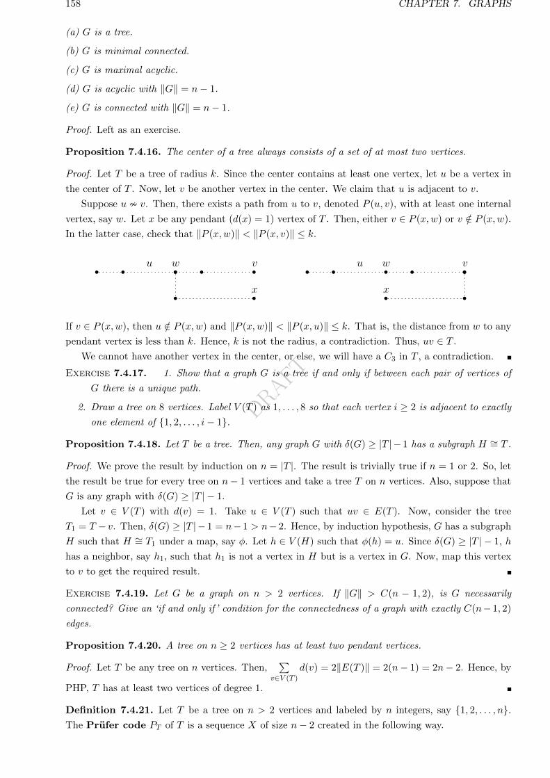
DRAFT


(a) G is a tree.

(b) G is minimal connected.

(c) G is maximal acyclic.

(d) G is acyclic with ‖G‖ = n− 1.

(e) G is connected with ‖G‖ = n− 1.

Proof. Left as an exercise.

Proposition 7.4.16. The center of a tree always consists of a set of at most two vertices.

Proof. Let T be a tree of radius k. Since the center contains at least one vertex, let u be a vertex in

the center of T . Now, let v be another vertex in the center. We claim that u is adjacent to v.

Suppose u v. Then, there exists a path from u to v, denoted P (u, v), with at least one internal

vertex, say w. Let x be any pendant (d(x) = 1) vertex of T . Then, either v ∈ P (x,w) or v /∈ P (x,w).

In the latter case, check that ‖P (x,w)‖ < ‖P (x, v)‖ ≤ k.

u w v

x

u w v

x

1

If v ∈ P (x,w), then u /∈ P (x,w) and ‖P (x,w)‖ < ‖P (x, u)‖ ≤ k. That is, the distance from w to any

pendant vertex is less than k. Hence, k is not the radius, a contradiction. Thus, uv ∈ T .

We cannot have another vertex in the center, or else, we will have a C3 in T , a contradiction.

Exercise 7.4.17. 1. Show that a graph G is a tree if and only if between each pair of vertices of

G there is a unique path.

2. Draw a tree on 8 vertices. Label V (T ) as 1, . . . , 8 so that each vertex i ≥ 2 is adjacent to exactly

one element of 1, 2, . . . , i− 1.

Proposition 7.4.18. Let T be a tree. Then, any graph G with δ(G) ≥ |T |− 1 has a subgraph H ∼= T .

Proof. We prove the result by induction on n = |T |. The result is trivially true if n = 1 or 2. So, let

the result be true for every tree on n− 1 vertices and take a tree T on n vertices. Also, suppose that

G is any graph with δ(G) ≥ |T | − 1.

Let v ∈ V (T ) with d(v) = 1. Take u ∈ V (T ) such that uv ∈ E(T ). Now, consider the tree

T1 = T − v. Then, δ(G) ≥ |T | − 1 = n− 1 > n− 2. Hence, by induction hypothesis, G has a subgraph

H such that H ∼= T1 under a map, say φ. Let h ∈ V (H) such that φ(h) = u. Since δ(G) ≥ |T | − 1, h

has a neighbor, say h1, such that h1 is not a vertex in H but is a vertex in G. Now, map this vertex

to v to get the required result.

Exercise 7.4.19. Let G be a graph on n > 2 vertices. If ‖G‖ > C(n − 1, 2), is G necessarily

connected? Give an ‘if and only if ’ condition for the connectedness of a graph with exactly C(n− 1, 2)

edges.

Proposition 7.4.20. A tree on n ≥ 2 vertices has at least two pendant vertices.

Proof. Let T be any tree on n vertices. Then,∑

v∈V (T )

d(v) = 2‖E(T )‖ = 2(n− 1) = 2n− 2. Hence, by

PHP, T has at least two vertices of degree 1.

Definition 7.4.21. Let T be a tree on n > 2 vertices and labeled by n integers, say 1, 2, . . . , n.The Prufer code PT of T is a sequence X of size n− 2 created in the following way.

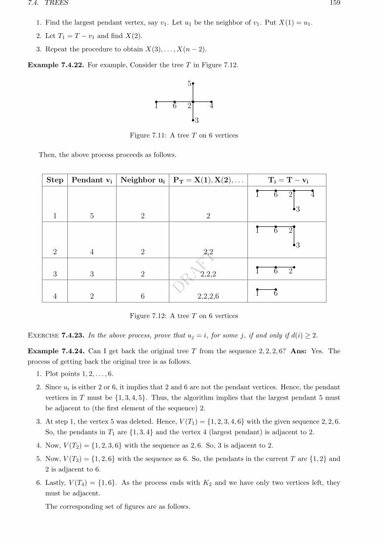
DRAFT

7.4. TREES 159

1. Find the largest pendant vertex, say v1. Let u1 be the neighbor of v1. Put X(1) = u1.

2. Let T1 = T − v1 and find X(2).

3. Repeat the procedure to obtain X(3), . . . , X(n− 2).

Example 7.4.22. For example, Consider the tree T in Figure 7.12.

1 2

3

4

5

6

Figure 7.11: A tree T on 6 vertices

Then, the above process proceeds as follows.

Step Pendant vi Neighbor ui PT = X(1),X(2), . . . Ti = T − vi

1 5 2 2

1 2

3

46

2 4 2 2,2

1 2

3

6

3 3 2 2,2,2 1 26

4 2 6 2,2,2,6 1 6

1

Figure 7.12: A tree T on 6 vertices

Exercise 7.4.23. In the above process, prove that uj = i, for some j, if and only if d(i) ≥ 2.

Example 7.4.24. Can I get back the original tree T from the sequence 2, 2, 2, 6? Ans: Yes. The

process of getting back the original tree is as follows.

1. Plot points 1, 2, . . . , 6.

2. Since ui is either 2 or 6, it implies that 2 and 6 are not the pendant vertices. Hence, the pendant

vertices in T must be 1, 3, 4, 5. Thus, the algorithm implies that the largest pendant 5 must

be adjacent to (the first element of the sequence) 2.

3. At step 1, the vertex 5 was deleted. Hence, V (T1) = 1, 2, 3, 4, 6 with the given sequence 2, 2, 6.

So, the pendants in T1 are 1, 3, 4 and the vertex 4 (largest pendant) is adjacent to 2.

4. Now, V (T2) = 1, 2, 3, 6 with the sequence as 2, 6. So, 3 is adjacent to 2.

5. Now, V (T3) = 1, 2, 6 with the sequence as 6. So, the pendants in the current T are 1, 2 and

2 is adjacent to 6.

6. Lastly, V (T4) = 1, 6. As the process ends with K2 and we have only two vertices left, they

must be adjacent.

The corresponding set of figures are as follows.

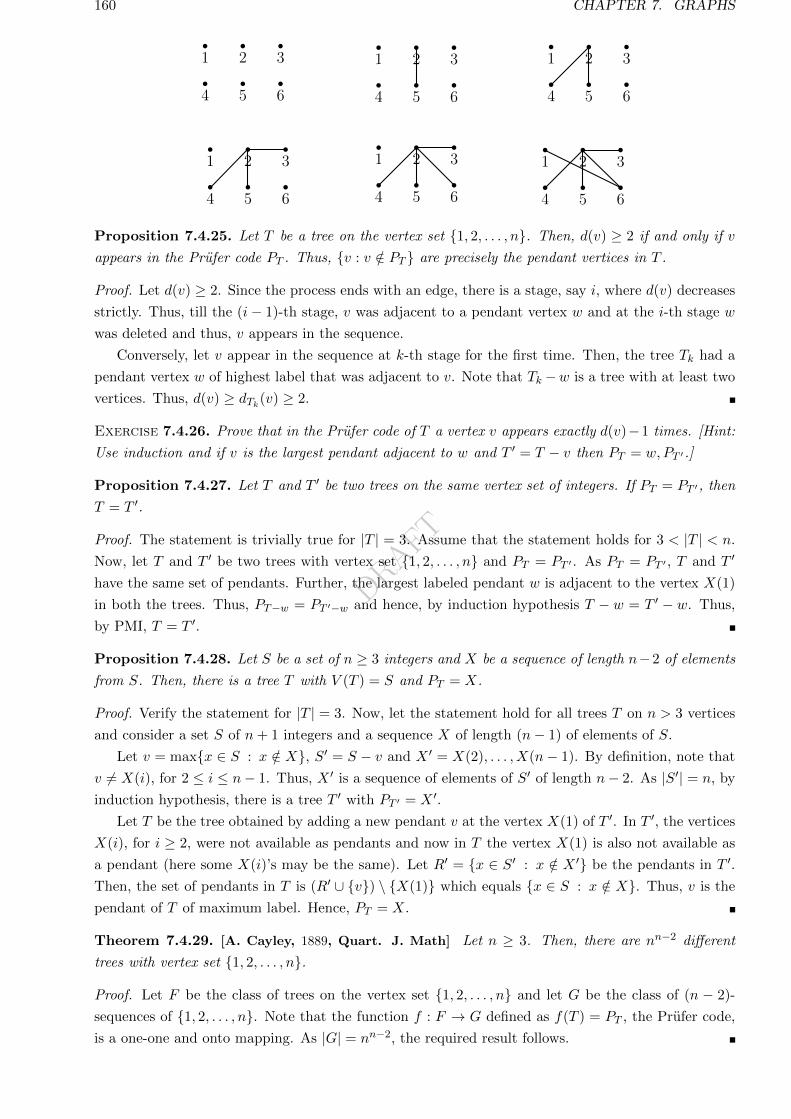
DRAFT


1 2 3

4 5 6

1 2 3

4 5 6

1 2 3

4 5 6

1 2 3

4 5 6

1 2 3

4 5 6

1 2 3

4 5 6

Proposition 7.4.25. Let T be a tree on the vertex set 1, 2, . . . , n. Then, d(v) ≥ 2 if and only if v

appears in the Prufer code PT . Thus, v : v /∈ PT are precisely the pendant vertices in T .

Proof. Let d(v) ≥ 2. Since the process ends with an edge, there is a stage, say i, where d(v) decreases

strictly. Thus, till the (i− 1)-th stage, v was adjacent to a pendant vertex w and at the i-th stage w

was deleted and thus, v appears in the sequence.

Conversely, let v appear in the sequence at k-th stage for the first time. Then, the tree Tk had a

pendant vertex w of highest label that was adjacent to v. Note that Tk −w is a tree with at least two

vertices. Thus, d(v) ≥ dTk(v) ≥ 2.

Exercise 7.4.26. Prove that in the Prufer code of T a vertex v appears exactly d(v)−1 times. [Hint:

Use induction and if v is the largest pendant adjacent to w and T ′ = T − v then PT = w,PT ′.]

Proposition 7.4.27. Let T and T ′ be two trees on the same vertex set of integers. If PT = PT ′, then

T = T ′.

Proof. The statement is trivially true for |T | = 3. Assume that the statement holds for 3 < |T | < n.

Now, let T and T ′ be two trees with vertex set 1, 2, . . . , n and PT = PT ′ . As PT = PT ′ , T and T ′

have the same set of pendants. Further, the largest labeled pendant w is adjacent to the vertex X(1)

in both the trees. Thus, PT−w = PT ′−w and hence, by induction hypothesis T − w = T ′ − w. Thus,

by PMI, T = T ′.

Proposition 7.4.28. Let S be a set of n ≥ 3 integers and X be a sequence of length n−2 of elements

from S. Then, there is a tree T with V (T ) = S and PT = X.

Proof. Verify the statement for |T | = 3. Now, let the statement hold for all trees T on n > 3 vertices

and consider a set S of n+ 1 integers and a sequence X of length (n− 1) of elements of S.

Let v = maxx ∈ S : x /∈ X, S′ = S − v and X ′ = X(2), . . . , X(n− 1). By definition, note that

v 6= X(i), for 2 ≤ i ≤ n− 1. Thus, X ′ is a sequence of elements of S′ of length n− 2. As |S′| = n, by

induction hypothesis, there is a tree T ′ with PT ′ = X ′.

Let T be the tree obtained by adding a new pendant v at the vertex X(1) of T ′. In T ′, the vertices

X(i), for i ≥ 2, were not available as pendants and now in T the vertex X(1) is also not available as

a pendant (here some X(i)’s may be the same). Let R′ = x ∈ S′ : x /∈ X ′ be the pendants in T ′.

Then, the set of pendants in T is (R′ ∪ v) \ X(1) which equals x ∈ S : x /∈ X. Thus, v is the

pendant of T of maximum label. Hence, PT = X.

Theorem 7.4.29. [A. Cayley, 1889, Quart. J. Math] Let n ≥ 3. Then, there are nn−2 different

trees with vertex set 1, 2, . . . , n.

Proof. Let F be the class of trees on the vertex set 1, 2, . . . , n and let G be the class of (n − 2)-

sequences of 1, 2, . . . , n. Note that the function f : F → G defined as f(T ) = PT , the Prufer code,

is a one-one and onto mapping. As |G| = nn−2, the required result follows.

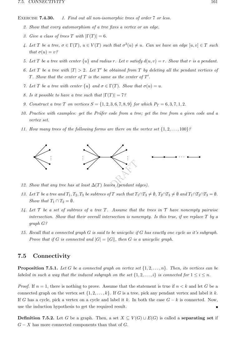
DRAFT

7.5. CONNECTIVITY 161

Exercise 7.4.30. 1. Find out all non-isomorphic trees of order 7 or less.

2. Show that every automorphism of a tree fixes a vertex or an edge.

3. Give a class of trees T with |Γ(T )| = 6.

4. Let T be a tree, σ ∈ Γ(T ), u ∈ V (T ) such that σ2(u) 6= u. Can we have an edge [u, v] ∈ T such

that σ(u) = v?

5. Let T be a tree with center u and radius r. Let v satisfy d(u, v) = r. Show that r is a pendant.

6. Let T be a tree with |T | > 2. Let T ′ be obtained from T by deleting all the pendant vertices of

T . Show that the center of T is the same as the center of T ′.

7. Let T be a tree with center u and σ ∈ Γ(T ). Show that σ(u) = u.

8. Is it possible to have a tree such that |Γ(T )| = 7?

9. Construct a tree T on vertices S = 1, 2, 3, 6, 7, 8, 9 for which PT = 6, 3, 7, 1, 2.

10. Practice with examples: get the Prufer code from a tree; get the tree from a given code and a

vertex set.

11. How many trees of the following forms are there on the vertex set 1, 2, . . . , 100?

......

... · · ·

1

12. Show that any tree has at least ∆(T ) leaves (pendant edges).

13. Let T be a tree and T1, T2, T3 be subtrees of T such that T1∩T3 6= ∅, T2∩T3 6= ∅ and T1∩T2∩T3 = ∅.Show that T1 ∩ T2 = ∅.

14. Let T be a set of subtrees of a tree T . Assume that the trees in T have nonempty pairwise

intersection. Show that their overall intersection is nonempty. Is this true, if we replace T by a

graph G?

15. Recall that a connected graph G is said to be unicyclic if G has exactly one cycle as it’s subgraph.

Prove that if G is connected and |G| = ‖G‖, then G is a unicyclic graph.

7.5 Connectivity

Proposition 7.5.1. Let G be a connected graph on vertex set 1, 2, . . . , n. Then, its vertices can be

labeled in such a way that the induced subgraph on the set 1, 2, . . . , i is connected for 1 ≤ i ≤ n.

Proof. If n = 1, there is nothing to prove. Assume that the statement is true if n < k and let G be a

connected graph on the vertex set 1, 2, . . . , k. If G is a tree, pick any pendant vertex and label it k.

If G has a cycle, pick a vertex on a cycle and label it k. In both the case G − k is connected. Now,

use the induction hypothesis to get the required result.

Definition 7.5.2. Let G be a graph. Then, a set X ⊆ V (G) ∪ E(G) is called a separating set if

G−X has more connected components than that of G.

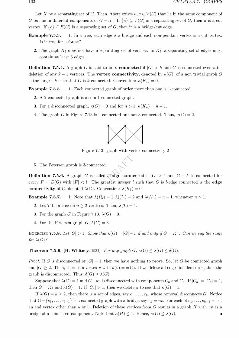
DRAFT


Let X be a separating set of G. Then, ‘there exists u, v ∈ V (G) that lie in the same component of

G but lie in different components of G−X’. If u ⊆ V (G) is a separating set of G, then u is a cut

vertex. If e ⊆ E(G) is a separating set of G, then it is a bridge/cut edge.

Example 7.5.3. 1. In a tree, each edge is a bridge and each non-pendant vertex is a cut vertex.

Is it true for a forest?

2. The graph K7 does not have a separating set of vertices. In K7, a separating set of edges must

contain at least 6 edges.

Definition 7.5.4. A graph G is said to be k-connected if |G| > k and G is connected even after

deletion of any k − 1 vertices. The vertex connectivity, denoted by κ(G), of a non trivial graph G

is the largest k such that G is k-connected. Convention: κ(K1) = 0.

Example 7.5.5. 1. Each connected graph of order more than one is 1-connected.

2. A 2-connected graph is also a 1-connected graph.

3. For a disconnected graph, κ(G) = 0 and for n > 1, κ(Kn) = n− 1.

4. The graph G in Figure 7.13 is 2-connected but not 3-connected. Thus, κ(G) = 2.

Figure 7.13: graph with vertex connectivity 2

5. The Petersen graph is 3-connected.

Definition 7.5.6. A graph G is called l-edge connected if |G| > 1 and G − F is connected for

every F ⊆ E(G) with |F | < l. The greatest integer l such that G is l-edge connected is the edge

connectivity of G, denoted λ(G). Convention: λ(K1) = 0.

Example 7.5.7. 1. Note that λ(Pn) = 1, λ(Cn) = 2 and λ(Kn) = n− 1, whenever n > 1.

2. Let T be a tree on n ≥ 2 vertices. Then, λ(T ) = 1.

3. For the graph G in Figure 7.13, λ(G) = 3.

4. For the Petersen graph G, λ(G) = 3.

Exercise 7.5.8. Let |G| > 1. Show that κ(G) = |G| − 1 if and only if G = Kn. Can we say the same

for λ(G)?

Theorem 7.5.9. [H. Whitney, 1932] For any graph G, κ(G) ≤ λ(G) ≤ δ(G).

Proof. If G is disconnected or |G| = 1, then we have nothing to prove. So, let G be connected graph

and |G| ≥ 2. Then, there is a vertex v with d(v) = δ(G). If we delete all edges incident on v, then the

graph is disconnected. Thus, δ(G) ≥ λ(G).

Suppose that λ(G) = 1 and G−uv is disconnected with components Cu and Cv. If |Cu| = |Cv| = 1,

then G = K2 and κ(G) = 1. If |Cu| > 1, then we delete u to see that κ(G) = 1.

If λ(G) = k ≥ 2, then there is a set of edges, say e1, . . . , ek, whose removal disconnects G. Notice

that G−e1, . . . , ek−1 is a connected graph with a bridge, say ek = uv. For each of e1, . . . , ek−1 select

an end vertex other than u or v. Deletion of these vertices from G results in a graph H with uv as a

bridge of a connected component. Note that κ(H) ≤ 1. Hence, κ(G) ≤ λ(G).

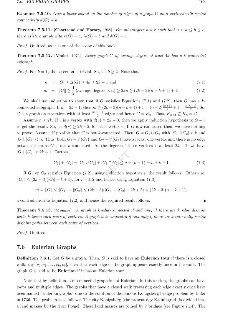
DRAFT

7.6. EULERIAN GRAPHS 163

Exercise 7.5.10. Give a lower bound on the number of edges of a graph G on n vertices with vertex

connectivity κ(G) = k.

Theorem 7.5.11. [Chartrand and Harary, 1968] For all integers a, b, c such that 0 < a ≤ b ≤ c,

there exists a graph with κ(G) = a, λ(G) = b and δ(G) = c.

Proof. Omitted, as it is out of the scope of this book.

Theorem 7.5.12. [Mader, 1972] Every graph G of average degree at least 4k has a k-connected

subgraph.

Proof. For k = 1, the assertion is trivial. So, let k ≥ 2. Note that

n = |G| ≥ ∆(G) ≥ 4k ≥ 2k − 1 and (7.1)

m = ‖G‖ ≥ 1

2(average degree × n) ≥ 2kn ≥ (2k − 3)(n− k + 1) + 1. (7.2)

We shall use induction to show that if G satisfies Equations (7.1) and (7.2), then G has a k-

connected subgraph. If n = 2k− 1, then m ≥ (2k− 3)(n− k+ 1) + 1 = (n− 2) (n+1)2 + 1 = n(n−1)

2 . So,

G is a graph on n vertices with at least n(n−1)2 edges and hence G = Kn. Thus, Kk+1 ⊆ Kn = G.

Assume n ≥ 2k. If v is a vertex with d(v) ≤ 2k − 3, then we apply induction hypothesis to G− vto get the result. So, let d(v) ≥ 2k − 2, for each vertex v. If G is k-connected then, we have nothing

to prove. Assume, if possible that G is not k-connected. Then, G = G1 ∪G2 with |G1 ∩G2| < k and

|G1|, |G2| < n. Thus, both G1 − V (G2) and G2 − V (G1) have at least one vertex and there is no edge

between them as G is not k-connected. As the degree of these vertices is at least 2k − 2, we have

|G1|, |G2| ≥ 2k − 1. Further,

|G1|+ |G2| = |G1 ∪G2|+ |G1 ∩G2| ≤ n+ (k − 1) = n+ k − 1. (7.3)

If G1 or G2 satisfies Equation (7.2), using induction hypothesis, the result follows. Otherwise,

‖Gi‖ ≤ (2k − 3)(|Gi| − k + 1), for i = 1, 2 and hence, using Equation (7.3)

m = ‖G‖ ≤ ‖G1‖+ ‖G2‖ ≤ (2k − 3)(|G1|+ |G2| − 2k + 2) ≤ (2k − 3)(n− k + 1),

a contradiction to Equation (7.2) and hence the required result follows.

Theorem 7.5.13. [Menger] A graph is k-edge-connected if and only if there are k edge disjoint

paths between each pairs of vertices. A graph is k-connected if and only if there are k internally vertex

disjoint paths between each pairs of vertices.

Proof. Omitted.

7.6 Eulerian Graphs

Definition 7.6.1. Let G be a graph. Then, G is said to have an Eulerian tour if there is a closed

walk, say [v0, v1, . . . , vk, v0], such that each edge of the graph appears exactly once in the walk. The

graph G is said to be Eulerian if it has an Eulerian tour.

Note that by definition, a disconnected graph is not Eulerian. In this section, the graphs can have

loops and multiple edges. The graphs that have a closed walk traversing each edge exactly once have

been named “Eulerian graphs” due to the solution of the famous Konigsberg bridge problem by Euler

in 1736. The problem is as follows: The city Konigsberg (the present day Kaliningrad) is divided into

4 land masses by the river Pregel. These land masses are joined by 7 bridges (see Figure 7.14). The

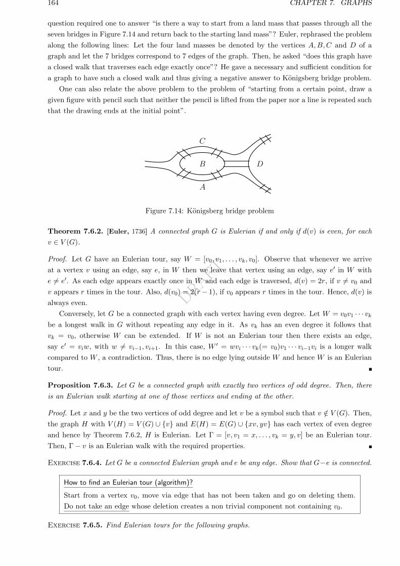
DRAFT


question required one to answer “is there a way to start from a land mass that passes through all the

seven bridges in Figure 7.14 and return back to the starting land mass”? Euler, rephrased the problem

along the following lines: Let the four land masses be denoted by the vertices A,B,C and D of a

graph and let the 7 bridges correspond to 7 edges of the graph. Then, he asked “does this graph have

a closed walk that traverses each edge exactly once”? He gave a necessary and sufficient condition for

a graph to have such a closed walk and thus giving a negative answer to Konigsberg bridge problem.

One can also relate the above problem to the problem of “starting from a certain point, draw a

given figure with pencil such that neither the pencil is lifted from the paper nor a line is repeated such

that the drawing ends at the initial point”.

B D

C

A

1

Figure 7.14: Konigsberg bridge problem

Theorem 7.6.2. [Euler, 1736] A connected graph G is Eulerian if and only if d(v) is even, for each

v ∈ V (G).

Proof. Let G have an Eulerian tour, say W = [v0, v1, . . . , vk, v0]. Observe that whenever we arrive

at a vertex v using an edge, say e, in W then we leave that vertex using an edge, say e′ in W with

e 6= e′. As each edge appears exactly once in W and each edge is traversed, d(v) = 2r, if v 6= v0 and

v appears r times in the tour. Also, d(v0) = 2(r− 1), if v0 appears r times in the tour. Hence, d(v) is

always even.

Conversely, let G be a connected graph with each vertex having even degree. Let W = v0v1 · · · vkbe a longest walk in G without repeating any edge in it. As vk has an even degree it follows that

vk = v0, otherwise W can be extended. If W is not an Eulerian tour then there exists an edge,

say e′ = viw, with w 6= vi−1, vi+1. In this case, W ′ = wvi · · · vk(= v0)v1 · · · vi−1vi is a longer walk

compared to W , a contradiction. Thus, there is no edge lying outside W and hence W is an Eulerian

tour.

Proposition 7.6.3. Let G be a connected graph with exactly two vertices of odd degree. Then, there

is an Eulerian walk starting at one of those vertices and ending at the other.

Proof. Let x and y be the two vertices of odd degree and let v be a symbol such that v /∈ V (G). Then,

the graph H with V (H) = V (G) ∪ v and E(H) = E(G) ∪ xv, yv has each vertex of even degree

and hence by Theorem 7.6.2, H is Eulerian. Let Γ = [v, v1 = x, . . . , vk = y, v] be an Eulerian tour.

Then, Γ− v is an Eulerian walk with the required properties.

Exercise 7.6.4. Let G be a connected Eulerian graph and e be any edge. Show that G−e is connected.

How to find an Eulerian tour (algorithm)?

Start from a vertex v0, move via edge that has not been taken and go on deleting them.

Do not take an edge whose deletion creates a non trivial component not containing v0.

Exercise 7.6.5. Find Eulerian tours for the following graphs.

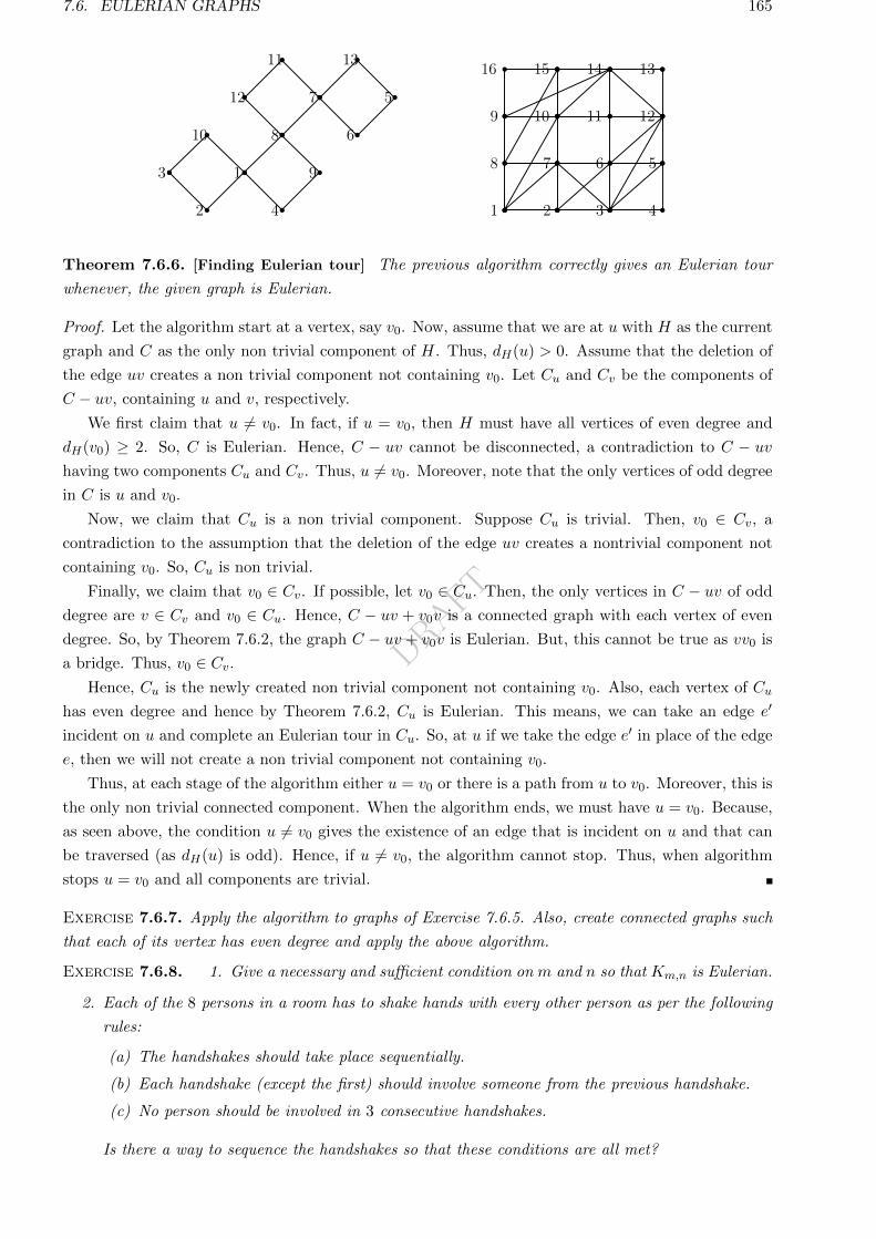
DRAFT

7.6. EULERIAN GRAPHS 165

8

1 2

7

3

6

4

5

9

16

12

15 13

11

14

10

3

2

1

4

9

8

7

6

5

1311

12

10

1

Theorem 7.6.6. [Finding Eulerian tour] The previous algorithm correctly gives an Eulerian tour

whenever, the given graph is Eulerian.

Proof. Let the algorithm start at a vertex, say v0. Now, assume that we are at u with H as the current

graph and C as the only non trivial component of H. Thus, dH(u) > 0. Assume that the deletion of

the edge uv creates a non trivial component not containing v0. Let Cu and Cv be the components of

C − uv, containing u and v, respectively.

We first claim that u 6= v0. In fact, if u = v0, then H must have all vertices of even degree and

dH(v0) ≥ 2. So, C is Eulerian. Hence, C − uv cannot be disconnected, a contradiction to C − uvhaving two components Cu and Cv. Thus, u 6= v0. Moreover, note that the only vertices of odd degree

in C is u and v0.

Now, we claim that Cu is a non trivial component. Suppose Cu is trivial. Then, v0 ∈ Cv, a

contradiction to the assumption that the deletion of the edge uv creates a nontrivial component not

containing v0. So, Cu is non trivial.

Finally, we claim that v0 ∈ Cv. If possible, let v0 ∈ Cu. Then, the only vertices in C − uv of odd

degree are v ∈ Cv and v0 ∈ Cu. Hence, C − uv + v0v is a connected graph with each vertex of even

degree. So, by Theorem 7.6.2, the graph C − uv + v0v is Eulerian. But, this cannot be true as vv0 is

a bridge. Thus, v0 ∈ Cv.Hence, Cu is the newly created non trivial component not containing v0. Also, each vertex of Cu

has even degree and hence by Theorem 7.6.2, Cu is Eulerian. This means, we can take an edge e′

incident on u and complete an Eulerian tour in Cu. So, at u if we take the edge e′ in place of the edge

e, then we will not create a non trivial component not containing v0.

Thus, at each stage of the algorithm either u = v0 or there is a path from u to v0. Moreover, this is

the only non trivial connected component. When the algorithm ends, we must have u = v0. Because,

as seen above, the condition u 6= v0 gives the existence of an edge that is incident on u and that can

be traversed (as dH(u) is odd). Hence, if u 6= v0, the algorithm cannot stop. Thus, when algorithm

stops u = v0 and all components are trivial.

Exercise 7.6.7. Apply the algorithm to graphs of Exercise 7.6.5. Also, create connected graphs such

that each of its vertex has even degree and apply the above algorithm.

Exercise 7.6.8. 1. Give a necessary and sufficient condition on m and n so that Km,n is Eulerian.

2. Each of the 8 persons in a room has to shake hands with every other person as per the following

rules:

(a) The handshakes should take place sequentially.

(b) Each handshake (except the first) should involve someone from the previous handshake.

(c) No person should be involved in 3 consecutive handshakes.

Is there a way to sequence the handshakes so that these conditions are all met?

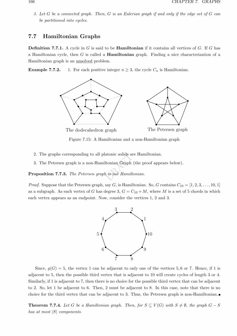
DRAFT


3. Let G be a connected graph. Then, G is an Eulerian graph if and only if the edge set of G can

be partitioned into cycles.

7.7 Hamiltonian Graphs

Definition 7.7.1. A cycle in G is said to be Hamiltonian if it contains all vertices of G. If G has

a Hamiltonian cycle, then G is called a Hamiltonian graph. Finding a nice characterization of a

Hamiltonian graph is an unsolved problem.

Example 7.7.2. 1. For each positive integer n ≥ 3, the cycle Cn is Hamiltonian.

The dodecahedron graph The Petersen graph

1

Figure 7.15: A Hamiltonian and a non-Hamiltonian graph

2. The graphs corresponding to all platonic solids are Hamiltonian.

3. The Petersen graph is a non-Hamiltonian Graph (the proof appears below).

Proposition 7.7.3. The Petersen graph is not Hamiltonian.

Proof. Suppose that the Petersen graph, say G, is Hamiltonian. So, G contains C10 = [1, 2, 3, . . . , 10, 1]

as a subgraph. As each vertex of G has degree 3, G = C10 +M , where M is a set of 5 chords in which

each vertex appears as an endpoint. Now, consider the vertices 1, 2 and 3.

1

23

4

5

6

7 8

9

10

Since, g(G) = 5, the vertex 1 can be adjacent to only one of the vertices 5, 6 or 7. Hence, if 1 is

adjacent to 5, then the possible third vertex that is adjacent to 10 will create cycles of length 3 or 4.

Similarly, if 1 is adjacent to 7, then there is no choice for the possible third vertex that can be adjacent

to 2. So, let 1 be adjacent to 6. Then, 2 must be adjacent to 8. In this case, note that there is no

choice for the third vertex that can be adjacent to 3. Thus, the Petersen graph is non-Hamiltonian.

Theorem 7.7.4. Let G be a Hamiltonian graph. Then, for S ⊆ V (G) with S 6= ∅, the graph G − Shas at most |S| components.

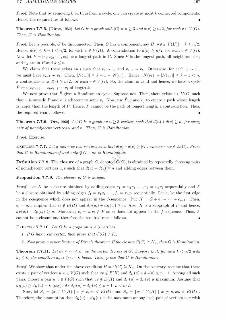
DRAFT

7.7. HAMILTONIAN GRAPHS 167

Proof. Note that by removing k vertices from a cycle, one can create at most k connected components.

Hence, the required result follows.

Theorem 7.7.5. [Dirac, 1952] Let G be a graph with |G| = n ≥ 3 and d(v) ≥ n/2, for each v ∈ V (G).

Then, G is Hamiltonian.

Proof. Let is possible, G be disconnected. Then, G has a component, say H, with |V (H)| = k ≤ n/2.

Hence, d(v) ≤ k − 1 < n/2, for each v ∈ V (H). A contradiction to d(v) ≥ n/2, for each v ∈ V (G).

Now, let P = [v1, v2, · · · , vk] be a longest path in G. Since P is the longest path, all neighbors of v1

and vk are in P and k ≤ n.

We claim that there exists an i such that v1 ∼ vi and vi−1 ∼ vk. Otherwise, for each vi ∼ v1,

we must have vi−1 vk. Then, |N(vk)| ≤ k − 1 − |N(v1)|. Hence, |N(v1)| + |N(vk)| ≤ k − 1 < n,

a contradiction to d(v) ≥ n/2, for each v ∈ V (G). So, the claim is valid and hence, we have a cycle

P := v1vivi+1 · · · vkvi−1 · · · v1 of length k.

We now prove that P gives a Hamiltonian cycle. Suppose not. Then, there exists v ∈ V (G) such

that v is outside P and v is adjacent to some vj . Now, use P , v and vj to create a path whose length

is larger than the length of P . Hence, P cannot be the path of longest length, a contradiction. Thus,


Theorem 7.7.6. [Ore, 1960] Let G be a graph on n ≥ 3 vertices such that d(u) + d(v) ≥ n, for every

pair of nonadjacent vertices u and v. Then, G is Hamiltonian.

Proof. Exercise.

Exercise 7.7.7. Let u and v be two vertices such that d(u)+d(v) ≥ |G|, whenever uv /∈ E(G). Prove

that G is Hamiltonian if and only if G+ uv is Hamiltonian.

Definition 7.7.8. The closure of a graph G, denoted C(G), is obtained by repeatedly choosing pairs

of nonadjacent vertices u, v such that d(u) + d(v) ≥ n and adding edges between them.

Proposition 7.7.9. The closure of G is unique.

Proof. Let K be a closure obtained by adding edges e1 = u1v1, . . . , ek = ukvk sequentially and F

be a closure obtained by adding edges f1 = x1y1, . . . , fr = xryr sequentially. Let ei be the first edge

in the e-sequence which does not appear in the f -sequence. Put H = G + e1 + · · · + ei−1. Then,

ei = uivi implies that ei /∈ E(H) and dH(ui) + dH(vi) ≥ n. Also, H is a subgraph of F and hence,

dF (ui) + dF (vi) ≥ n. Moreover, ei = uivi /∈ F as ei does not appear in the f -sequence. Thus, F

cannot be a closure and therefore the required result follows.

Exercise 7.7.10. Let G be a graph on n ≥ 3 vertices.

1. If G has a cut vertex, then prove that C(G) 6= Kn.

2. Now prove a generalization of Dirac’s theorem: If the closure C(G) ∼= Kn, then G is Hamiltonian.

Theorem 7.7.11. Let d1 ≤ · · · ≤ dn be the vertex degrees of G. Suppose that, for each k < n/2 with

dk ≤ k, the condition dn−k ≥ n− k holds. Then, prove that G is Hamiltonian.

Proof. We show that under the above condition H = C(G) ∼= Kn. On the contrary, assume that there

exists a pair of vertices u, v ∈ V (G) such that uv /∈ E(H) and dH(u) +dH(v) ≤ n−1. Among all such

pairs, choose a pair u, v ∈ V (G) such that uv /∈ E(H) and dH(u) + dH(v) is maximum. Assume that

dH(v) ≥ dH(u) = k (say). As dH(u) + dH(v) ≤ n− 1, k < n/2.

Now, let Sv = x ∈ V (H) | x 6= v, xv /∈ E(H) and Su = w ∈ V (H) | w 6= u,wu /∈ E(H).Therefore, the assumption that dH(u) + dH(v) is the maximum among each pair of vertices u, v with

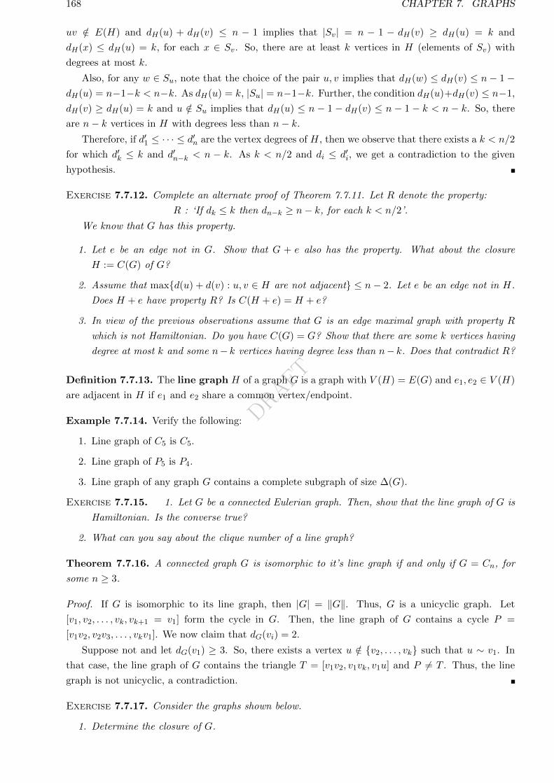
DRAFT


uv /∈ E(H) and dH(u) + dH(v) ≤ n − 1 implies that |Sv| = n − 1 − dH(v) ≥ dH(u) = k and

dH(x) ≤ dH(u) = k, for each x ∈ Sv. So, there are at least k vertices in H (elements of Sv) with

degrees at most k.

Also, for any w ∈ Su, note that the choice of the pair u, v implies that dH(w) ≤ dH(v) ≤ n− 1−dH(u) = n−1−k < n−k. As dH(u) = k, |Su| = n−1−k. Further, the condition dH(u)+dH(v) ≤ n−1,

dH(v) ≥ dH(u) = k and u /∈ Su implies that dH(u) ≤ n − 1 − dH(v) ≤ n − 1 − k < n − k. So, there

are n− k vertices in H with degrees less than n− k.

Therefore, if d′1 ≤ · · · ≤ d′n are the vertex degrees of H, then we observe that there exists a k < n/2

for which d′k ≤ k and d′n−k < n − k. As k < n/2 and di ≤ d′i, we get a contradiction to the given

hypothesis.

Exercise 7.7.12. Complete an alternate proof of Theorem 7.7.11. Let R denote the property:

R : ‘If dk ≤ k then dn−k ≥ n− k, for each k < n/2’.

We know that G has this property.

1. Let e be an edge not in G. Show that G + e also has the property. What about the closure

H := C(G) of G?

2. Assume that maxd(u) + d(v) : u, v ∈ H are not adjacent ≤ n− 2. Let e be an edge not in H.

Does H + e have property R? Is C(H + e) = H + e?

3. In view of the previous observations assume that G is an edge maximal graph with property R

which is not Hamiltonian. Do you have C(G) = G? Show that there are some k vertices having

degree at most k and some n− k vertices having degree less than n− k. Does that contradict R?

Definition 7.7.13. The line graph H of a graph G is a graph with V (H) = E(G) and e1, e2 ∈ V (H)

are adjacent in H if e1 and e2 share a common vertex/endpoint.

Example 7.7.14. Verify the following:

1. Line graph of C5 is C5.

2. Line graph of P5 is P4.

3. Line graph of any graph G contains a complete subgraph of size ∆(G).

Exercise 7.7.15. 1. Let G be a connected Eulerian graph. Then, show that the line graph of G is

Hamiltonian. Is the converse true?

2. What can you say about the clique number of a line graph?

Theorem 7.7.16. A connected graph G is isomorphic to it’s line graph if and only if G = Cn, for

some n ≥ 3.

Proof. If G is isomorphic to its line graph, then |G| = ‖G‖. Thus, G is a unicyclic graph. Let

[v1, v2, . . . , vk, vk+1 = v1] form the cycle in G. Then, the line graph of G contains a cycle P =

[v1v2, v2v3, . . . , vkv1]. We now claim that dG(vi) = 2.

Suppose not and let dG(v1) ≥ 3. So, there exists a vertex u /∈ v2, . . . , vk such that u ∼ v1. In

that case, the line graph of G contains the triangle T = [v1v2, v1vk, v1u] and P 6= T . Thus, the line

graph is not unicyclic, a contradiction.

Exercise 7.7.17. Consider the graphs shown below.

1. Determine the closure of G.

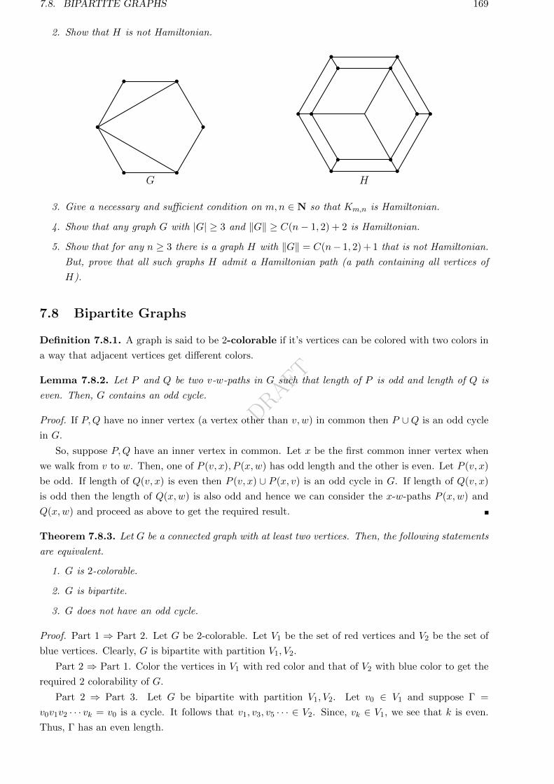
DRAFT

7.8. BIPARTITE GRAPHS 169

2. Show that H is not Hamiltonian.

G H

3. Give a necessary and sufficient condition on m,n ∈ N so that Km,n is Hamiltonian.

4. Show that any graph G with |G| ≥ 3 and ‖G‖ ≥ C(n− 1, 2) + 2 is Hamiltonian.

5. Show that for any n ≥ 3 there is a graph H with ‖G‖ = C(n− 1, 2) + 1 that is not Hamiltonian.

But, prove that all such graphs H admit a Hamiltonian path (a path containing all vertices of

H).

7.8 Bipartite Graphs

Definition 7.8.1. A graph is said to be 2-colorable if it’s vertices can be colored with two colors in

a way that adjacent vertices get different colors.

Lemma 7.8.2. Let P and Q be two v-w-paths in G such that length of P is odd and length of Q is

even. Then, G contains an odd cycle.

Proof. If P,Q have no inner vertex (a vertex other than v, w) in common then P ∪Q is an odd cycle

in G.

So, suppose P,Q have an inner vertex in common. Let x be the first common inner vertex when

we walk from v to w. Then, one of P (v, x), P (x,w) has odd length and the other is even. Let P (v, x)

be odd. If length of Q(v, x) is even then P (v, x) ∪ P (x, v) is an odd cycle in G. If length of Q(v, x)

is odd then the length of Q(x,w) is also odd and hence we can consider the x-w-paths P (x,w) and

Q(x,w) and proceed as above to get the required result.

Theorem 7.8.3. Let G be a connected graph with at least two vertices. Then, the following statements

are equivalent.

1. G is 2-colorable.

2. G is bipartite.

3. G does not have an odd cycle.

Proof. Part 1 ⇒ Part 2. Let G be 2-colorable. Let V1 be the set of red vertices and V2 be the set of

blue vertices. Clearly, G is bipartite with partition V1, V2.

Part 2 ⇒ Part 1. Color the vertices in V1 with red color and that of V2 with blue color to get the

required 2 colorability of G.

Part 2 ⇒ Part 3. Let G be bipartite with partition V1, V2. Let v0 ∈ V1 and suppose Γ =

v0v1v2 · · · vk = v0 is a cycle. It follows that v1, v3, v5 · · · ∈ V2. Since, vk ∈ V1, we see that k is even.

Thus, Γ has an even length.

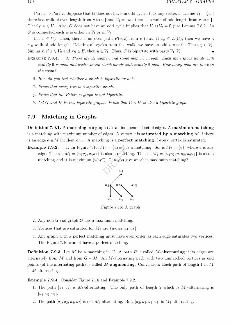
DRAFT


Part 3⇒ Part 2. Suppose that G does not have an odd cycle. Pick any vertex v. Define V1 = w |there is a walk of even length from v to w and V2 = w | there is a walk of odd length from v to w.Clearly, v ∈ V1. Also, G does not have an odd cycle implies that V1 ∩ V2 = ∅ (use Lemma 7.8.2. As

G is connected each w is either in V1 or in V2.

Let x ∈ V1. Then, there is an even path P (v, x) from v to x. If xy ∈ E(G), then we have a

v-y-walk of odd length. Deleting all cycles from this walk, we have an odd v-y-path. Thus, y ∈ V2.Similarly, if x ∈ V2 and xy ∈ E, then y ∈ V1. Thus, G is bipartite with parts V1, V2.

Exercise 7.8.4. 1. There are 15 women and some men in a room. Each man shook hands with

exactly 6 women and each woman shook hands with exactly 8 men. How many men are there in

the room?

2. How do you test whether a graph is bipartite or not?

3. Prove that every tree is a bipartite graph.

4. Prove that the Petersen graph is not bipartite.

5. Let G and H be two bipartite graphs. Prove that G×H is also a bipartite graph.

7.9 Matching in Graphs

Definition 7.9.1. A matching in a graph G is an independent set of edges. A maximum matching

is a matching with maximum number of edges. A vertex v is saturated by a matching M if there

is an edge e ∈M incident on v. A matching is a perfect matching if every vertex is saturated.

Example 7.9.2. 1. In Figure 7.16, M1 = u1u2 is a matching. So, is M2 = e, where e is any

edge. The set M3 = u3u2, u4u7 is also a matching. The set M4 = u1u2, u4u5, u6u7 is also a

matching and it is maximum (why?). Can you give another maximum matching?

u1

u2

u3 u4 u5

u6u7

Figure 7.16: A graph

2. Any non trivial graph G has a maximum matching.

3. Vertices that are saturated for M3 are u2, u3, u4, u7.4. Any graph with a perfect matching must have even order as each edge saturates two vertices.

The Figure 7.16 cannot have a perfect matching.

Definition 7.9.3. Let M be a matching in G. A path P is called M-alternating if its edges are

alternately from M and from G −M . An M -alternating path with two unmatched vertices as end

points (of the alternating path) is called M-augmenting. Convention: Each path of length 1 in M

is M -alternating.

Example 7.9.4. Consider Figure 7.16 and Example 7.9.2.

1. The path [u1, u2] is M1-alternating. The only path of length 2 which is M1-alternating is

[u1, u2, u3].

2. The path [u1, u2, u4, u7] is not M3-alternating. But, [u2, u3, u4, u7] is M3-alternating.

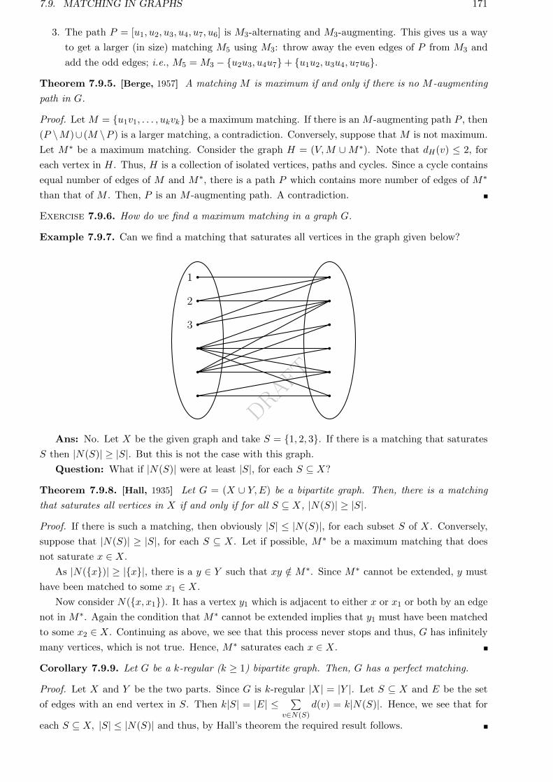
DRAFT

7.9. MATCHING IN GRAPHS 171

3. The path P = [u1, u2, u3, u4, u7, u6] is M3-alternating and M3-augmenting. This gives us a way

to get a larger (in size) matching M5 using M3: throw away the even edges of P from M3 and

add the odd edges; i.e., M5 = M3 − u2u3, u4u7+ u1u2, u3u4, u7u6.

Theorem 7.9.5. [Berge, 1957] A matching M is maximum if and only if there is no M -augmenting

path in G.

Proof. Let M = u1v1, . . . , ukvk be a maximum matching. If there is an M -augmenting path P , then

(P \M)∪ (M \P ) is a larger matching, a contradiction. Conversely, suppose that M is not maximum.

Let M∗ be a maximum matching. Consider the graph H = (V,M ∪M∗). Note that dH(v) ≤ 2, for

each vertex in H. Thus, H is a collection of isolated vertices, paths and cycles. Since a cycle contains

equal number of edges of M and M∗, there is a path P which contains more number of edges of M∗

than that of M . Then, P is an M -augmenting path. A contradiction.

Exercise 7.9.6. How do we find a maximum matching in a graph G.

Example 7.9.7. Can we find a matching that saturates all vertices in the graph given below?

1

2

3

Ans: No. Let X be the given graph and take S = 1, 2, 3. If there is a matching that saturates

S then |N(S)| ≥ |S|. But this is not the case with this graph.

Question: What if |N(S)| were at least |S|, for each S ⊆ X?

Theorem 7.9.8. [Hall, 1935] Let G = (X ∪ Y,E) be a bipartite graph. Then, there is a matching

that saturates all vertices in X if and only if for all S ⊆ X, |N(S)| ≥ |S|.

Proof. If there is such a matching, then obviously |S| ≤ |N(S)|, for each subset S of X. Conversely,

suppose that |N(S)| ≥ |S|, for each S ⊆ X. Let if possible, M∗ be a maximum matching that does

not saturate x ∈ X.

As |N(x)| ≥ |x|, there is a y ∈ Y such that xy /∈ M∗. Since M∗ cannot be extended, y must

have been matched to some x1 ∈ X.

Now consider N(x, x1). It has a vertex y1 which is adjacent to either x or x1 or both by an edge

not in M∗. Again the condition that M∗ cannot be extended implies that y1 must have been matched

to some x2 ∈ X. Continuing as above, we see that this process never stops and thus, G has infinitely

many vertices, which is not true. Hence, M∗ saturates each x ∈ X.

Corollary 7.9.9. Let G be a k-regular (k ≥ 1) bipartite graph. Then, G has a perfect matching.

Proof. Let X and Y be the two parts. Since G is k-regular |X| = |Y |. Let S ⊆ X and E be the set

of edges with an end vertex in S. Then k|S| = |E| ≤ ∑v∈N(S)

d(v) = k|N(S)|. Hence, we see that for

each S ⊆ X, |S| ≤ |N(S)| and thus, by Hall’s theorem the required result follows.

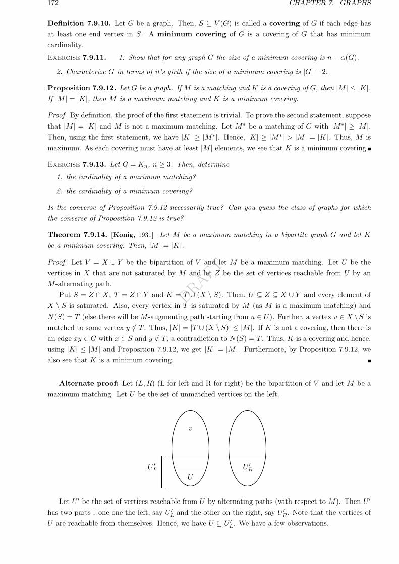
DRAFT


Definition 7.9.10. Let G be a graph. Then, S ⊆ V (G) is called a covering of G if each edge has

at least one end vertex in S. A minimum covering of G is a covering of G that has minimum

cardinality.

Exercise 7.9.11. 1. Show that for any graph G the size of a minimum covering is n− α(G).

2. Characterize G in terms of it’s girth if the size of a minimum covering is |G| − 2.

Proposition 7.9.12. Let G be a graph. If M is a matching and K is a covering of G, then |M | ≤ |K|.If |M | = |K|, then M is a maximum matching and K is a minimum covering.

Proof. By definition, the proof of the first statement is trivial. To prove the second statement, suppose

that |M | = |K| and M is not a maximum matching. Let M∗ be a matching of G with |M∗| ≥ |M |.Then, using the first statement, we have |K| ≥ |M∗|. Hence, |K| ≥ |M∗| > |M | = |K|. Thus, M is

maximum. As each covering must have at least |M | elements, we see that K is a minimum covering.

Exercise 7.9.13. Let G = Kn, n ≥ 3. Then, determine

1. the cardinality of a maximum matching?

2. the cardinality of a minimum covering?

Is the converse of Proposition 7.9.12 necessarily true? Can you guess the class of graphs for which

the converse of Proposition 7.9.12 is true?

Theorem 7.9.14. [Konig, 1931] Let M be a maximum matching in a bipartite graph G and let K

be a minimum covering. Then, |M | = |K|.

Proof. Let V = X ∪ Y be the bipartition of V and let M be a maximum matching. Let U be the

vertices in X that are not saturated by M and let Z be the set of vertices reachable from U by an

M -alternating path.

Put S = Z ∩X, T = Z ∩ Y and K = T ∪ (X \ S). Then, U ⊆ Z ⊆ X ∪ Y and every element of

X \ S is saturated. Also, every vertex in T is saturated by M (as M is a maximum matching) and

N(S) = T (else there will be M -augmenting path starting from u ∈ U). Further, a vertex v ∈ X \S is

matched to some vertex y /∈ T . Thus, |K| = |T ∪ (X \ S)| ≤ |M |. If K is not a covering, then there is

an edge xy ∈ G with x ∈ S and y /∈ T , a contradiction to N(S) = T . Thus, K is a covering and hence,

using |K| ≤ |M | and Proposition 7.9.12, we get |K| = |M |. Furthermore, by Proposition 7.9.12, we

also see that K is a minimum covering.

Alternate proof: Let (L,R) (L for left and R for right) be the bipartition of V and let M be a

maximum matching. Let U be the set of unmatched vertices on the left.

U

U ′L U ′

R

v

1

Let U ′ be the set of vertices reachable from U by alternating paths (with respect to M). Then U ′

has two parts : one one the left, say U ′L and the other on the right, say U ′R. Note that the vertices of

U are reachable from themselves. Hence, we have U ⊆ U ′L. We have a few observations.

DRAFT

7.10. RAMSEY NUMBERS 173

a) If v ∈ L is a left vertex not in U ′L, then it is not in U , and so it must be matched to some right

vertex, say w. Can w ∈ U ′R? No. Because, if w ∈ U ′R, then we have an alternating path from u to

w and as [w, u] is a matching edge, we see that v is reachable from u by an alternating path. Then

v should have been in U ′L, a contradiction. Thus every vertex from L \ U ′L is matched to a vertex in

R \ U ′R.

b) Is every vertex in U ′R matched (saturated)? Yes. To see it, suppose that w ∈ U ′R is not matched.

As w ∈ U ′R, it must be reachable from a vertex u ∈ U via an alternating path. But, this alternating

path is an augmenting path. This means M is not a maximum matching, a contradiction.

c) The above two points imply that |M | = |L \ U ′L|+ |U ′R|.d) Is there any edge from a vertex in U ′L to a vertex in R \ U ′R? No. To see this note that, each

vertex in U ′L \ U is reached from some vertex of U via an alternating path and the last edge of this

path must be a matching edge. Thus, each vertex in U ′L \ U is matched to some vertex in U ′R. This

means, if there an edge from a vertex in U ′L to a vertex in w ∈ R\U ′R, it must be a nonmatching edge.

But then, this makes w reachable from U via an alternating path. So w should have been in U ′R, a

contradiction.

e) The previous point means that (L \ U ′L) ∪ U ′R is covering. This is a minimum covering, as any

covering must contain at least |M | many vertices by Proposition 7.9.12.

Exercise 7.9.15. How many perfect matchings are there in a labeled K2n?

7.10 Ramsey Numbers

Recall that in any group of 6 or more persons either we see 3 mutual friends or we see 3 mutual

strangers. Expressed using graphs it reads ‘let G = (V,E) be a graph with |V | ≥ 6. Then, either

K3 ⊆ G or K3 ⊆ G.’

Definition 7.10.1. The Ramsey number r(m,n) is the smallest natural number k such that any

graph G on k vertices either has a Km or a Kn as it’s subgraph.

Example 7.10.2. As C5 does not have K3 or K3 as it’s subgraph, r(3, 3) > 5. But, using the first

paragraph of this section, we get r(3, 3) ≤ 6 and hence, r(3, 3) = 6. It is known that r(3, 4) = 9 (see

the text by Harary for a table).

Proposition 7.10.3. Let G be a graph on 9 vertices. Then, either K4 ⊆ G or K3 ⊆ G.

Proof. Assume that |V | = 9. Then, we need to consider three cases.

Case I. There is a vertex a with d(v) ≤ 4. Then, |N(a)′| = |V \N(a)| ≥ 4. If all vertices in N(a)′

are pairwise adjacent, then K4 ⊆ G. Otherwise, there are two nonadjacent vertices, say b, c ∈ N(a)′.

In that case a, b, c induces the graph K3.

Case II. There is a vertex a with d(a) ≥ 6. If 〈N(a)〉 has a K3, we are done. Otherwise, r(3, 3) = 6

implies that 〈N(a)〉 has a K3 with vertices, say, b, c, d. In that case a, b, c, d induces the graph K4.

Case III. Each vertex has degree 5. This case is not possible as∑d(v) should be even.

Exercise 7.10.4. Can you draw a graph on 8 vertices

1. which does not have K3,K4 in it?

2. which does not have K4,K3 in it?

3. Consider the graph C8 = [1, 2, . . . , 8, 1] with 10 extra edges 13, 14, 17, 26, 27, 35, 36, 48, 57, 58.

Does this graph has a K4 or the complement of C3?

DRAFT


Theorem 7.10.5. [Erdos & Szekeres, 1935] Let m,n ∈ N. Then,

r(m,n) ≤ r(m− 1, n) + r(m,n− 1).

Proof. Let p = r(m − 1, n) and q = r(m,n − 1). Now, take any graph G on p + q vertices and take

a vertex a. If d(a) ≥ p, then 〈N(a)〉 has either a subgraph Km−1 (and Km−1 together with a gives

Km) or a subgraph Kn. Otherwise, |N(a)′| ≥ q. In this case, 〈N(a)′〉 has either a subgraph Km or a

subgraph Kn−1 (Kn−1 together with a gives Kn).

7.11 Degree Sequence

Definition 7.11.1. The degree sequence of a graph of order n is the tuple (d1, . . . , dn) where

d1 ≤ · · · ≤ dn. A non-decreasing sequence d = (d1, . . . , dn) of non-negative integers is graphic if there

is a graph whose degree sequence is d.

Exercise 7.11.2. Show that (1, 1, 3, 3) is not graphic.

Theorem 7.11.3. Fix n ≥ 1 and the natural numbers d1 ≤ · · · ≤ dn. Then, d = (d1, . . . , dn) is the

degree sequence of a tree on n vertices if and only if∑di = 2n− 2.

Proof. If d = (d1, . . . , dn) is the degree sequence of a tree on n vertices then∑di = 2|E(T )| =

2(n− 1) = 2n− 2.

Conversely, let d1 ≤ · · · ≤ dn be a sequence of natural numbers with∑di = 2n − 2. We use

induction to show that d = (d1, . . . , dn) is the degree sequence of a tree on n vertices. For n = 1, 2, the

result is trivial. Let the result be true for all n < k and let d1 ≤ · · · ≤ dk, k > 2, be natural numbers

with∑di = 2k − 2. Since,

∑di = 2k − 2, we must have d1 = 1 and dk > 1. Then, we note that

d′2 = d2, · · · , d′k−1 = dk−1 and d′k = dk − 1 are natural numbers such that∑d′i = 2(k− 1)− 2. Hence,

by induction hypothesis, there is a tree T ′ on vertices 2, · · · , k−1, k with degrees d′i’s. Now, introduce

a new vertex 1 and add the edge 1, k to get a tree T that has the required degree sequence.

Theorem 7.11.4. [Havel-Hakimi, 1962] The degree sequence d = (d1, . . . , dn) is graphic if and only

if the sequence d1, d2, . . . , dn−dn−1, dn−dn − 1, . . . , dn−1 − 1 is graphic.

Proof. If the later sequence is graphic then we introduce a new vertex and make it adjacent to the

vertices whose degrees are dn−dn − 1, . . . , dn−1 − 1. Hence, the sequence d = (d1, . . . , dn) is graphic.

Now, assume that d is graphic and G is a graph with degree sequence d. Let dn = k and let

NG(n) = i1, i2, . . . , ik with di1 ≤ di2 ≤ · · · ≤ dik . If di1 ≥ dv for all v ∈ V (G) \ NG(n) then

di1 , di2 , . . . , dik = dn−dn , dn−dn+1, . . . , dn−1 and hence G− n is the required graph.

If di1 < dv0 for some v0 ∈ V (G) \ NG(n) then, we construct another graph, say G′, such that G

and G′ have the same degree sequence but∑v∈NG′ (n)

dv ≥∑

u∈NG(n)du. (7.4)

As, v0 6∼ n, the vertex v0 has a neighbor v 6= i1 with v 6∼ i1. Now, consider the graph G′ =

G − v0, v + n, v0 + i1, v − i1, n. Then, G′ also has d as it’s degree sequence with NG′(n) =

v0, i2, . . . , ik. Thus, we see that Equation (7.4) holds. This process will end after a finite number

of steps by producing a graph in which the vertex n has degree dn and has neighbors with degrees

dn−dn , dn−dn+1, . . . , dn−1 and hence the required result follows.

Exercise 7.11.5. 1. How many different degree sequences are possible on a graph with 5 vertices?

List all the degree sequences and draw a graph for each one. (Include connected and disconnected

graphs.)

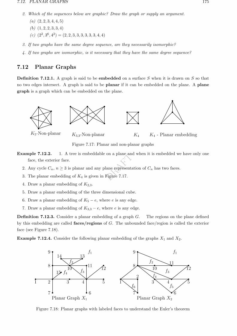
DRAFT

7.12. PLANAR GRAPHS 175

2. Which of the sequences below are graphic? Draw the graph or supply an argument.

(a) (2, 2, 3, 4, 4, 5)

(b) (1, 2, 2, 3, 3, 4)

(c) (22, 36, 42) = (2, 2, 3, 3, 3, 3, 3, 3, 4, 4)

3. If two graphs have the same degree sequence, are they necessarily isomorphic?

4. If two graphs are isomorphic, is it necessary that they have the same degree sequence?

7.12 Planar Graphs

Definition 7.12.1. A graph is said to be embedded on a surface S when it is drawn on S so that

no two edges intersect. A graph is said to be planar if it can be embedded on the plane. A plane

graph is a graph which can be embedded on the plane.

K5-Non-planar K3,3-Non-planar K4 K4 - Planar embedding

1

Figure 7.17: Planar and non-planar graphs

Example 7.12.2. 1. A tree is embeddable on a plane and when it is embedded we have only one

face, the exterior face.

2. Any cycle Cn, n ≥ 3 is planar and any plane representation of Cn has two faces.

3. The planar embedding of K4 is given in Figure 7.17.

4. Draw a planar embedding of K2,3.

5. Draw a planar embedding of the three dimensional cube.

6. Draw a planar embedding of K5 − e, where e is any edge.

7. Draw a planar embedding of K3,3 − e, where e is any edge.

Definition 7.12.3. Consider a planar embedding of a graph G. The regions on the plane defined

by this embedding are called faces/regions of G. The unbounded face/region is called the exterior

face (see Figure 7.18).

Example 7.12.4. Consider the following planar embedding of the graphs X1 and X2.

15

3 4 51 2

6

8

9

1011

12

7

1314f1

f2

f3f4

Planar Graph X1

3 4 512

6

8

9

1011

12

7

f1

f2

f3

f4

f5f6

Planar Graph X2

1

Figure 7.18: Planar graphs with labeled faces to understand the Euler’s theorem

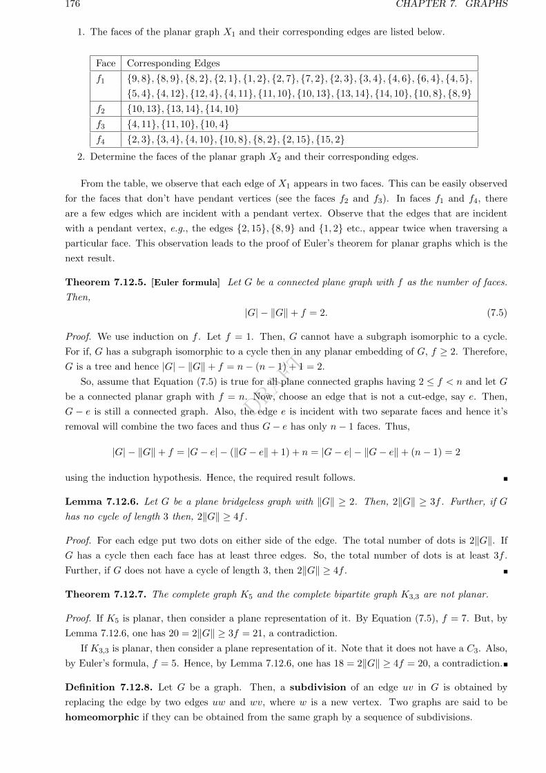
DRAFT


1. The faces of the planar graph X1 and their corresponding edges are listed below.

Face Corresponding Edges

f1 9, 8, 8, 9, 8, 2, 2, 1, 1, 2, 2, 7, 7, 2, 2, 3, 3, 4, 4, 6, 6, 4, 4, 5,5, 4, 4, 12, 12, 4, 4, 11, 11, 10, 10, 13, 13, 14, 14, 10, 10, 8, 8, 9

f2 10, 13, 13, 14, 14, 10f3 4, 11, 11, 10, 10, 4f4 2, 3, 3, 4, 4, 10, 10, 8, 8, 2, 2, 15, 15, 2

2. Determine the faces of the planar graph X2 and their corresponding edges.

From the table, we observe that each edge of X1 appears in two faces. This can be easily observed

for the faces that don’t have pendant vertices (see the faces f2 and f3). In faces f1 and f4, there

are a few edges which are incident with a pendant vertex. Observe that the edges that are incident

with a pendant vertex, e.g., the edges 2, 15, 8, 9 and 1, 2 etc., appear twice when traversing a

particular face. This observation leads to the proof of Euler’s theorem for planar graphs which is the

next result.

Theorem 7.12.5. [Euler formula] Let G be a connected plane graph with f as the number of faces.

Then,

|G| − ‖G‖+ f = 2. (7.5)

Proof. We use induction on f . Let f = 1. Then, G cannot have a subgraph isomorphic to a cycle.

For if, G has a subgraph isomorphic to a cycle then in any planar embedding of G, f ≥ 2. Therefore,

G is a tree and hence |G| − ‖G‖+ f = n− (n− 1) + 1 = 2.

So, assume that Equation (7.5) is true for all plane connected graphs having 2 ≤ f < n and let G

be a connected planar graph with f = n. Now, choose an edge that is not a cut-edge, say e. Then,

G − e is still a connected graph. Also, the edge e is incident with two separate faces and hence it’s

removal will combine the two faces and thus G− e has only n− 1 faces. Thus,

|G| − ‖G‖+ f = |G− e| − (‖G− e‖+ 1) + n = |G− e| − ‖G− e‖+ (n− 1) = 2

using the induction hypothesis. Hence, the required result follows.

Lemma 7.12.6. Let G be a plane bridgeless graph with ‖G‖ ≥ 2. Then, 2‖G‖ ≥ 3f . Further, if G

has no cycle of length 3 then, 2‖G‖ ≥ 4f .

Proof. For each edge put two dots on either side of the edge. The total number of dots is 2‖G‖. If

G has a cycle then each face has at least three edges. So, the total number of dots is at least 3f .

Further, if G does not have a cycle of length 3, then 2‖G‖ ≥ 4f .

Theorem 7.12.7. The complete graph K5 and the complete bipartite graph K3,3 are not planar.

Proof. If K5 is planar, then consider a plane representation of it. By Equation (7.5), f = 7. But, by

Lemma 7.12.6, one has 20 = 2‖G‖ ≥ 3f = 21, a contradiction.

If K3,3 is planar, then consider a plane representation of it. Note that it does not have a C3. Also,

by Euler’s formula, f = 5. Hence, by Lemma 7.12.6, one has 18 = 2‖G‖ ≥ 4f = 20, a contradiction.

Definition 7.12.8. Let G be a graph. Then, a subdivision of an edge uv in G is obtained by

replacing the edge by two edges uw and wv, where w is a new vertex. Two graphs are said to be

homeomorphic if they can be obtained from the same graph by a sequence of subdivisions.

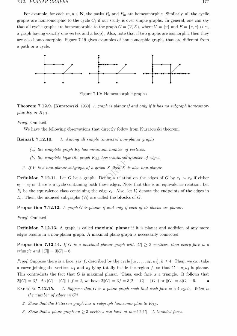
DRAFT

7.12. PLANAR GRAPHS 177

For example, for each m,n ∈ N, the paths Pn and Pm are homeomorphic. Similarly, all the cyclic

graphs are homeomorphic to the cycle C3 if our study is over simple graphs. In general, one can say

that all cyclic graphs are homeomorphic to the graph G = (V,E), where V = v and E = e, e (i.e.,

a graph having exactly one vertex and a loop). Also, note that if two graphs are isomorphic then they

are also homeomorphic. Figure 7.19 gives examples of homeomorphic graphs that are different from

a path or a cycle.

1

Figure 7.19: Homeomorphic graphs

Theorem 7.12.9. [Kuratowski, 1930] A graph is planar if and only if it has no subgraph homeomor-

phic K5 or K3,3.

Proof. Omitted.

We have the following observations that directly follow from Kuratowski theorem.

Remark 7.12.10. 1. Among all simple connected non-planar graphs

(a) the complete graph K5 has minimum number of vertices.

(b) the complete bipartite graph K3,3 has minimum number of edges.

2. If Y is a non-planar subgraph of a graph X then X is also non-planar.

Definition 7.12.11. Let G be a graph. Define a relation on the edges of G by e1 ∼ e2 if either

e1 = e2 or there is a cycle containing both these edges. Note that this is an equivalence relation. Let

Ei be the equivalence class containing the edge ei. Also, let Vi denote the endpoints of the edges in

Ei. Then, the induced subgraphs 〈Vi〉 are called the blocks of G.

Proposition 7.12.12. A graph G is planar if and only if each of its blocks are planar.

Proof. Omitted.

Definition 7.12.13. A graph is called maximal planar if it is planar and addition of any more

edges results in a non-planar graph. A maximal plane graph is necessarily connected.

Proposition 7.12.14. If G is a maximal planar graph with |G| ≥ 3 vertices, then every face is a

triangle and ‖G‖ = 3|G| − 6.

Proof. Suppose there is a face, say f , described by the cycle [u1, . . . , uk, u1], k ≥ 4. Then, we can take

a curve joining the vertices u1 and u3 lying totally inside the region f , so that G + u1u3 is planar.

This contradicts the fact that G is maximal planar. Thus, each face is a triangle. It follows that

2‖G‖ = 3f . As |G| − ‖G‖+ f = 2, we have 2‖G‖ = 3f = 3(2− |G|+ ‖G‖) or ‖G‖ = 3|G| − 6.

Exercise 7.12.15. 1. Suppose that G is a plane graph such that each face is a 4-cycle. What is

the number of edges in G?

2. Show that the Petersen graph has a subgraph homeomorphic to K3,3.

3. Show that a plane graph on ≥ 3 vertices can have at most 2|G| − 5 bounded faces.

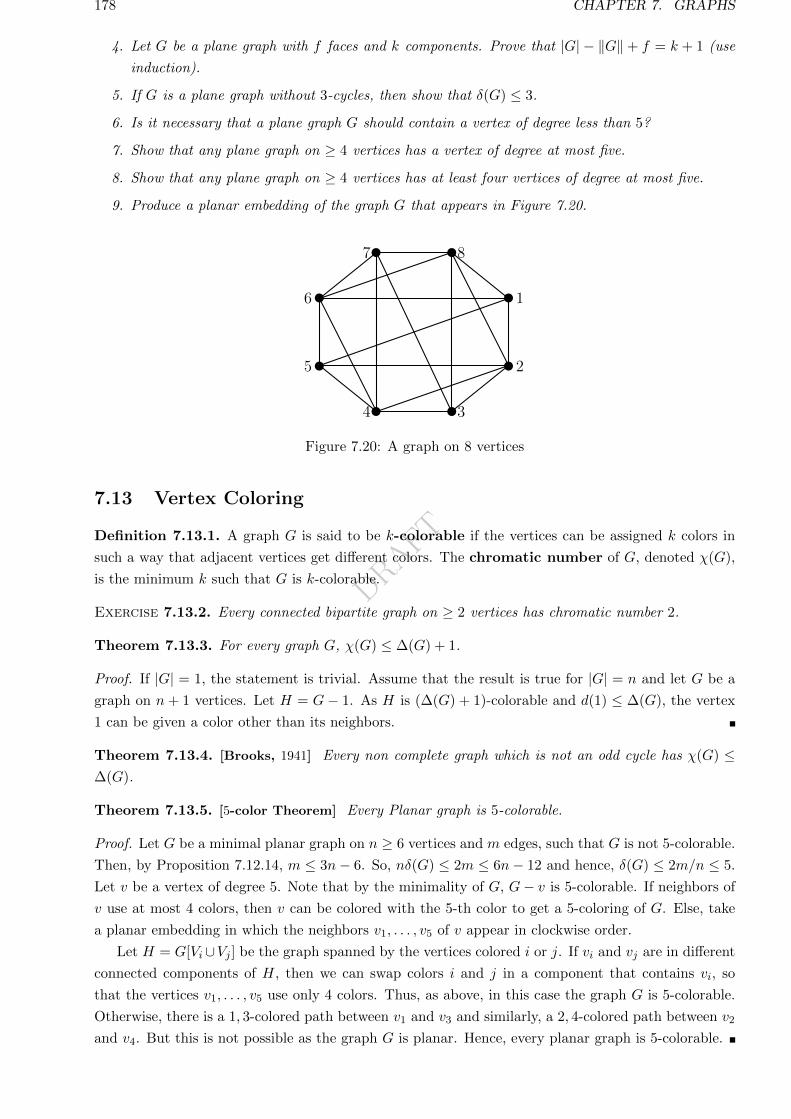
DRAFT


4. Let G be a plane graph with f faces and k components. Prove that |G| − ‖G‖+ f = k + 1 (use

induction).

5. If G is a plane graph without 3-cycles, then show that δ(G) ≤ 3.

6. Is it necessary that a plane graph G should contain a vertex of degree less than 5?

7. Show that any plane graph on ≥ 4 vertices has a vertex of degree at most five.

8. Show that any plane graph on ≥ 4 vertices has at least four vertices of degree at most five.

9. Produce a planar embedding of the graph G that appears in Figure 7.20.

1

2

3

8

6

5

4

7

1

Figure 7.20: A graph on 8 vertices

7.13 Vertex Coloring

Definition 7.13.1. A graph G is said to be k-colorable if the vertices can be assigned k colors in

such a way that adjacent vertices get different colors. The chromatic number of G, denoted χ(G),

is the minimum k such that G is k-colorable.

Exercise 7.13.2. Every connected bipartite graph on ≥ 2 vertices has chromatic number 2.

Theorem 7.13.3. For every graph G, χ(G) ≤ ∆(G) + 1.

Proof. If |G| = 1, the statement is trivial. Assume that the result is true for |G| = n and let G be a

graph on n+ 1 vertices. Let H = G− 1. As H is (∆(G) + 1)-colorable and d(1) ≤ ∆(G), the vertex

1 can be given a color other than its neighbors.

Theorem 7.13.4. [Brooks, 1941] Every non complete graph which is not an odd cycle has χ(G) ≤∆(G).

Theorem 7.13.5. [5-color Theorem] Every Planar graph is 5-colorable.

Proof. Let G be a minimal planar graph on n ≥ 6 vertices and m edges, such that G is not 5-colorable.

Then, by Proposition 7.12.14, m ≤ 3n− 6. So, nδ(G) ≤ 2m ≤ 6n− 12 and hence, δ(G) ≤ 2m/n ≤ 5.

Let v be a vertex of degree 5. Note that by the minimality of G, G− v is 5-colorable. If neighbors of

v use at most 4 colors, then v can be colored with the 5-th color to get a 5-coloring of G. Else, take

a planar embedding in which the neighbors v1, . . . , v5 of v appear in clockwise order.

Let H = G[Vi∪Vj ] be the graph spanned by the vertices colored i or j. If vi and vj are in different

connected components of H, then we can swap colors i and j in a component that contains vi, so

that the vertices v1, . . . , v5 use only 4 colors. Thus, as above, in this case the graph G is 5-colorable.

Otherwise, there is a 1, 3-colored path between v1 and v3 and similarly, a 2, 4-colored path between v2

and v4. But this is not possible as the graph G is planar. Hence, every planar graph is 5-colorable.

DRAFT

7.14. REPRESENTING GRAPHS WITH MATRICES 179

7.14 Representing graphs with Matrices

Definition 7.14.1. Let G = (V,E) be a simple (undirected) graph on vertices 1, . . . , n. Then, the

adjacency matrix A(G) of G (or simply A) is described by

aij =

1 if i, j ∈ E,0 otherwise.

Let H be the graph obtained by relabeling the vertices of G. Then, note that A(H) = S−1A(G)S,

for some permutation matrix S (recall that for a permutation matrix St = S−1). Hence, we talk of

the adjacency matrix of a graph and do not worry about the labeling of the vertices of G.

Example 7.14.2. The adjacency matrices of the 4-cycle C4 and the path P4 on 4 vertices are given

below.

A(C4) =

0 1 0 1

1 0 1 0

0 1 0 1

1 0 1 0

, A(P4) =

0 1 0 0

1 0 1 0

0 1 0 1

0 0 1 0

.Exercise 7.14.3. 1. A graph G is not connected if and only if there exists a permutation matrix

P such that A(G) =

[A11 0

0 A22

], for some matrices A11 and A22.

2. Two graphs G and H are isomorphic if and only if A(G) = P tA(H)P , for some permutation

matrix P .

Theorem 7.14.4. The (i, j) entry of B = A(G)k is the number of i-j-walks of length k.

Proof. Note that by the definition of matrix product

bij =∑

i1,...,ik−1

aii1ai1i2 · · · aik−1ik .

Thus, bij = r if and only if we have r sequences i1, . . . , ik−1 with aii1 = · · · = aik−1ik = 1. That is,

bij = r if and only if we have r walks of length k between i and j.

Theorem 7.14.5. Let G be a graph of order n. Then, G is connected if and only if[I +A(G)

]n−1is

entrywise positive.

Proof. PutB = I+A and letG be connected. If P is an i-j-path of length n−1, thenBn−1ij ≥ An−1ij ≥ 1.

If P = [i, i1, . . . , ik = j] is an i-j-path of length k < n− 1, then bii . . . biibii1 . . . bik−1j = 1, where bii is

used n− 1− k times. Thus, Bn−1ij > 0.

Conversely, let Bn−1ij > 0. Then, the corresponding summand bii1 . . . bin−1j is positive. By throwing

out entries of the form bii, for 1 ≤ i ≤ n, from this expression, we have an expression which corresponds

to an i-j-walk of length at most n− 1. As Bn−1 is entrywise positive, it follows that G is connected.

Exercise 7.14.6. Let G be a simple, undirected graph with adjacency matrix A.

1. Then the eigenvalues of A are all real.

2. The eigenvectors can be chosen to form an orthonormal basis of Rn.

3. If A has a rational eigenvalue then it has to be an integer.

4. If G be the complete graph Kn then A = J−I, where J is the matrix with each entry 1. Further,

in this case n − 1 is an eigenvalues with multiplicity 1 and −1 as an eigenvalue repeated n − 1

times.

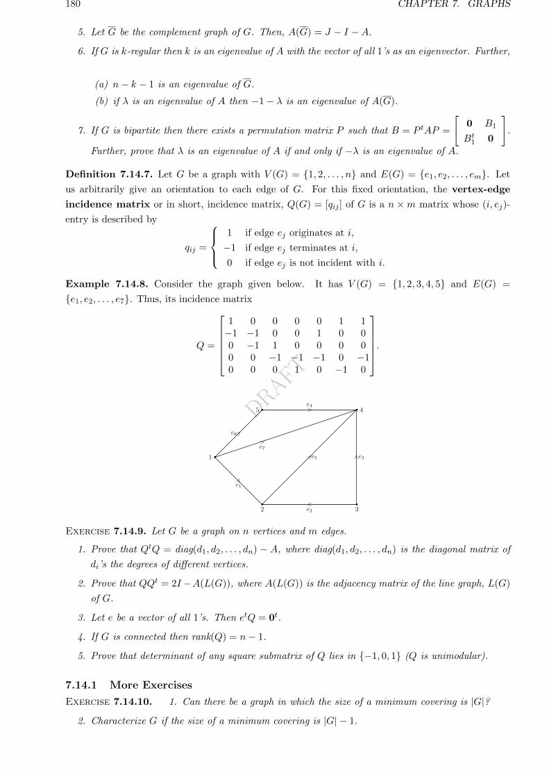
DRAFT


5. Let G be the complement graph of G. Then, A(G) = J − I −A.

6. If G is k-regular then k is an eigenvalue of A with the vector of all 1’s as an eigenvector. Further,

(a) n− k − 1 is an eigenvalue of G.

(b) if λ is an eigenvalue of A then −1− λ is an eigenvalue of A(G).

7. If G is bipartite then there exists a permutation matrix P such that B = P tAP =

[0 B1

Bt1 0

].

Further, prove that λ is an eigenvalue of A if and only if −λ is an eigenvalue of A.

Definition 7.14.7. Let G be a graph with V (G) = 1, 2, . . . , n and E(G) = e1, e2, . . . , em. Let

us arbitrarily give an orientation to each edge of G. For this fixed orientation, the vertex-edge

incidence matrix or in short, incidence matrix, Q(G) = [qij ] of G is a n ×m matrix whose (i, ej)-

entry is described by

qij =

1 if edge ej originates at i,

−1 if edge ej terminates at i,

0 if edge ej is not incident with i.

Example 7.14.8. Consider the graph given below. It has V (G) = 1, 2, 3, 4, 5 and E(G) =

e1, e2, . . . , e7. Thus, its incidence matrix

Q =

1 0 0 0 0 1 1−1 −1 0 0 1 0 00 −1 1 0 0 0 00 0 −1 −1 −1 0 −10 0 0 1 0 −1 0

.

<

>

>

>

>

>>

1

2 3

45

e2

e3

e1

e4

e5

e6

e7

1

Exercise 7.14.9. Let G be a graph on n vertices and m edges.

1. Prove that QtQ = diag(d1, d2, . . . , dn) − A, where diag(d1, d2, . . . , dn) is the diagonal matrix of

di’s the degrees of different vertices.

2. Prove that QQt = 2I−A(L(G)), where A(L(G)) is the adjacency matrix of the line graph, L(G)

of G.

3. Let e be a vector of all 1’s. Then etQ = 0t.

4. If G is connected then rank(Q) = n− 1.

5. Prove that determinant of any square submatrix of Q lies in −1, 0, 1 (Q is unimodular).

7.14.1 More Exercises

Exercise 7.14.10. 1. Can there be a graph in which the size of a minimum covering is |G|?2. Characterize G if the size of a minimum covering is |G| − 1.

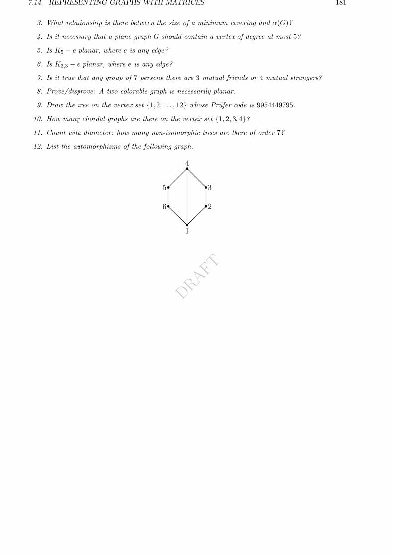
DRAFT

7.14. REPRESENTING GRAPHS WITH MATRICES 181

3. What relationship is there between the size of a minimum covering and α(G)?

4. Is it necessary that a plane graph G should contain a vertex of degree at most 5?

5. Is K5 − e planar, where e is any edge?

6. Is K3,3 − e planar, where e is any edge?

7. Is it true that any group of 7 persons there are 3 mutual friends or 4 mutual strangers?

8. Prove/disprove: A two colorable graph is necessarily planar.

9. Draw the tree on the vertex set 1, 2, . . . , 12 whose Prufer code is 9954449795.

10. How many chordal graphs are there on the vertex set 1, 2, 3, 4?11. Count with diameter: how many non-isomorphic trees are there of order 7?

12. List the automorphisms of the following graph.

1

2

3

4

5

6

DRAFT


DRAFT

Bibliography

[1] G. Agnarson and R. Greenlaw, Graph Theory: Modelling, Applications and Algorithm, Pearson

Education.

[2] R. B. Bapat, Graphs and Matrices, Hindustan Book Agency, New Delhi, 2010.

[3] J. Cofman, “Catalan Numbers for the Classroom?”, Elem. Math., 52 (1997), 108 - 117.

[4] D. M. Cvetkovic, Michael Doob and Horst Sachs, Spectra of Graphs: theory and applications,

Academic Press, New York, 1980.

[5] D. I. A. Cohen, Basic Techniques of Combinatorial Theory, John Wiley and Sons, New York,

1978.

[6] William Dunham, Euler: The Master of Us All, Published and Distributed by The Mathematical

Association of America, 1999.

[7] F. Harary, Graph Theory, Addison-Wesley Publishing Company, 1969.

[8] Victor J Katz, A history of mathematics, an intro, Harper Collins College Publishers, New York,

1993.

[9] G. E. Martin, Counting: The Art of Enumerative Combinatorics, Undergraduate Texts in Math-

ematics, Springer, 2001.

[10] R. Merris, Combinatorics, 2th edition, Wiley-Interscience, 2003.

[11] J. Riordan, Introduction to Combinatorial Analysis, John Wiley and Sons, New York, 1958.

[12] R. P. Stanley, Enumerative Combinatorics, vol. 2, Cambridge University Press, 1999.

[13] H. S. Wilf, Generatingfunctionology, Academic Press, 1990.

183

DRAFT

Index

C(G): Closure of G, 167

P (n;n1, . . . , nk), 80

∆(G): Maximum degree of G, 148

α(G): Independence number of G, 146

cf[xn, f ] : Coefficient of xn in f , 107

δ(G): Minimum degree of G, 148

diam(G): Diameter of G, 151

κ(G): Vertex connectivity of G, 162

〈U〉: Induced subgraph on U , 148

λ(G): Edge connectivity of G, 162

ω(G): Clique number of G, 153

ε(G): Edge density of G, 153

−1, 0, 1 vertex-edge incidence matrix, 180

f1, . . . , fn ⇒ g, 136

g(G): Girth of G, 151

n-set, 78

r-combination, 80

r-permutation, 78

r-sequence, 78

Absolute value in Z, 53

Algebraic expansion, 83

Anti-chain

Width, 58

Argument, 127

Atomic formula, 127

Atomic variable, 127

Axiom of Choice, 62

Equivalent Axioms, 63

Bezout’s identity, 43

Bell Numbers, 122

Bell numbers, 94

Bijective function, 14

Bipartite graph, 146

Blocks of a graph, 177

Boolean algebra, 71

Absorption, 72

Atom, 73

Free, 72

Homomorphism, 73

Idempotence, 72

Identity elements, 71

Induced partial order, 73

Inverse, 71

Isomorphism, 73

Principle of duality, 72

Cardinal numbers

Product, 65

Sum, 65

Cartesian Product, 9

Catalan number (Cn), 97

Cauchy product, 107

Chain, 58

Height, 58

Chinese remainder theorem, 48

Circuit in a graph, 151

Circular permutation, 84

Clique in a graph, 153

Coin problem, 114

Combination

C(n, r), 80

connected permutation, 116

Contradiction and tautology, 130

Countably finite, 34

Countably infinite, 34

Counting

Addition rule, 77

Multiplication rule, 77

Cycle in a graph, 151

Chord, 152

Degree sequence, 174

Graphic, 174

Derangement, 105

Difference equation, 116

k-th difference, 116

First difference, 116

Disconnect graph, 153

Distributive lattice, 66

Division algorithm, 42

184

DRAFT

INDEX 185

Durfee square, 115

Empty Set, 6

Equivalence relation, 17

Equivalent Sets, 14

Euclid’s Algorithm, 43

Euclid’s lemma, 45

Euler’s totient function (ϕ(n)), 105

Eulerian graph, 163

Eulerian tour, 163

Factorial

Falling, 79

Falling (xn), 95

Rising (xn), 95

Family of finite character, 62

Family of sets, 19

Intersection, 19

Union, 19

Ferrer’s diagram, 112

Conjugate, 113

Self conjugate, 113

Fibonacci sequence, 116

Finite set, 34

Cardinality, 33

Forest, 156

Formal power series

Cauchy product, 107

differentiation, 110

Equality, 107

integration, 110

Reciprocal, 109

Sum, 107

Formal power series (P(x)), 107

Formula

p implies q, 129

x-bound part, 139

Adequate, 132

Assignment, 128

Atomic, 140

bound, 139

Conclusion, 136

Conjunction, 128

Conjunctive normal form (CNF), 134

Connectives, 130

Contradiction, 130

Contrapositive, 130

Converse, 130

Disjunction, 128

Disjunctive normal form (DNF), 134

Dual, 134

Equivalent, 131

free, 139

Functionally complete, 132

Hypothesis, 136

Interpretation, 140

Literal, 134

Logical conclusion, 136

Negation, 128

Order of operations, 135

Polish notation, 135

Premise, 136

Principal connective, 134

Quantifier, 139

Satisfiable, 135

Substitution instance, 131

tautology, 130

Truth function, 130

Well formed, 130

Frobenius number, 114

Function

Bijective, 14

Domain, 12

Identity, 13

Image, 11

Injective, 14

Multiplicative, 106

One-one, 14

Onto, 14

Partial, 11

Pre-image, 11

Range, 12

Restriction, 14

Surjective, 14

Total, 12

Zero, 13

Fundamental theorem of arithmetic, 45

Generating function

Bell numbers, 122

Binomial coefficients, 121

Catalan numbers, 120

Stirling numbers (S(n, k)), 121

Generating functions

DRAFT

186 INDEX

Exponential (egf), 108

Ordinary (ogf), 108

Graph, 145

2-colorable, 169

M -Alternating path, 170

M -Augmenting path, 170

k-colorable, 178

k-factor, 148

Acyclic, 152

Addition of edge, 149

Adjacency matrix, 179

Adjacent vertices, 146

Automorphism, 155

Automorphism group, 155

Bipartite, 146

Blocks, 177

Bridge, 156

Cartesian product, 150

Center, 151

Chord, 152

Chordal, 152

Chromatic number (χ(G)), 178

Clique, 153

Clique number (ω(G)), 153

Closed path, 151

Closed trail, 151

Closure (C(G)), 167

Coloring, 178

Complement, 149

Complete (Kn), 146

Complete bipartite (Kr,s), 146

Component, 153

Connected, 153

Connected component, 153

Covering, 172

Cubic, 148

Cut edge, 156

Cut vertex, 156

Cycle (Cn), 146

Degree (d(v), dG(v)), 146

Degree sequence, 174

Diameter (diam(G)), 151

Disconnected, 153

Disjoint union, 149

Distance, 151

Edge connectivity (λ(G)), 162

Edge deleted, 149

Edge density (ε(G)), 153

Edge set (E,E(G)), 145

Embedding, 175

End vertex, 145

Eulerian, 163

Forest, 156

Girth (g(G)), 151

Hamiltonian, 166

Homeomorphic, 176

Incident edge, 145

Independence number (α(G)), 146

Independent set, 146

Induced subgraph (〈U〉), 148

Intersection, 149

Invariant, 155

Isolated vertices, 146

Isomorphism, 154

Join, 150

Length of path, 151

Length of walk, 151

Line graph, 168

Loop, 145

Matching, 170

Maximal, 152

Maximal planar, 177

Maximum degree (∆(G)), 148

Maximum matching, 170

Minimal, 152

Minimum covering, 172

Minimum degree (δ(G)), 148

Neighbor (N(v), NG(v)), 146

Path (Pn), 146

Pendant, 146

Perfect matching, 170

Petersen, 148

Planar, 175

Radius, 151

Regular, 148

Self-complimentary, 154

Separating set, 161

Simple, 146

Spanning subgraph, 148

Subdivision, 176

Subgraph, 148

Trail, 151

DRAFT

INDEX 187

Tree, 156

Trivial, 146

Union, 149

Vertex connectivity (κ(G)), 162

Vertex deleted, 149

Vertex set (V, V (G)), 145

Walk, 151

Graphic sequence, 174

Hamel basis, 63

Hamiltonian graph, 166

Hand shaking lemma, 147

Hasse diagram, 59

Directed, 58

Hypergraph, 146

Identity function, 13

Induced partial order, 63

Inductive Set, 24

Infinite Set, 34

Initial segment, 61

Injective function, 14

Integers

Co-prime, 43

Composite, 45

Divisibility, 43

Divisor, 43

Greatest common divisor (gcd), 43

Highest common factor, 43

Least common multiple (lcm), 46

Modular arithmetic, 46

Prime, 45

Relatively prime, 43

Unity, 45

Inverse Relation, 11

Isomorphic graphs, 154

Join of two graphs, 150

Lattice, 66

n-tuples of 0 and 1, 67

Bounded, 69

Complement, 69

Complete, 68

Direct product, 67

Distributive, 66

Homomorphism, 68

Isomorphism, 68

Lattice path, 95

Lemma

Hand shaking, 147

LHRRCC, 116

Line graph, 168

Linear congruence, 47

Linear Diophantine equation, 44

Linear recurrence relation, 116

Homogeneous, 116

Nonhomogeneous, 116

Linearly ordered set, 58

LNHRRCC, 116

Matching

Saturated vertex, 170

Mathematical induction, 28

Modulus in Z, 53

Money changing problem, 114

Multigraph, 146

Multiplicative function, 106

Multiset, 79

Natural number

Square-free, 75

Natural Numbers

Addition, 24

Multiplication, 24

Newton’s identity, 82

Null Set, 6

Number of r-permutations, 78

Number of circular permutations, 85

One-one correspondence, 14

One-one function, 14

Onto function, 14

Orbit, 85

Orbit size, 85

Order

Complete, 58

Dictionary, 58

Lexicographic, 58

Linear, 58

Total, 58

Ordering in N, 26

Partial function, 11

Domain, 12

Range, 12

DRAFT

188 INDEX

Partial order, 57

Comparable, 57

Induced, 63

Partially ordered set, 57

Partition of n (πn), 95

Partition of n into k parts (πn(k)), 95

Partition of a Set, 18

Path in a graph, 151

End vertices, 151

Internal vertices, 151

Peanos Axioms, 23

Addition in Q, 54

Addition in Z, 50

Construction of Q, 54

Construction of Z, 50

Division in Q, 54

Multiplication in Q, 54

Multiplication in Z, 51

Non-negative elements in Z, 53

Order in Q, 55

Order in Z, 52

Permutation, 78

P (n, r), 79

Circular, 84

Petersen graph, 148

Pigeonhole principle (PHP), 101

Planar graph, 175

Edges, 175

Exterior face, 175

Faces, 175

Maximal, 177

Regions, 175

Plane graph, 175

Poset

Anti-chain, 58

Chain, 58

Greatest lower bound (glb), 60

Height, 58

Least upper bound (lub), 60

Lower bound, 60

Maximal element, 60

Maximum element, 60

Minimal element, 60

Minimum element, 60

Upper bound, 60

Width, 58

Positive elements in Z, 53

Power set, 9

Uncountable, 41

Prufer code, 158

Predicate, 139

Principle of mathematical induction, 28

Principle of transfinite induction, 61

Product of sets, 62

Propositional function, 139

Pseudograph, 145

Quantified formula

Equivalent, 141

Valid, 141

Quantifier, 139

Scope, 139

Ramsey number (r(m,n)), 173

Recurrence relation, 116

Characteristic equation, 117

General solution-Distinct roots, 117

General solution-Multiple roots, 118

Initial condition, 116

Solution, 116

Recursive Theorem, 28

Relation, 10

Anti-symmetric, 16

Equivalence, 17

Inverse, 11

Reflexive, 16

Symmetric, 16

Transitive, 16

Restricted function, 14

Rotation, 85

Schroder-Bernstein Theorem, 39

Scope of quatifier, 139

Sequence, 36

Set

Cartesian Product, 9

Complement, 9

Composition of Relations, 15

Difference, 8

Disjoint, 7

Empty, 6

Enumeration, 36

Equality, 7

Family, 19

DRAFT

INDEX 189

Finite, 34

Identity Relation, 13

Inductive, 24

Infinite, 34

Intersection, 7

Null, 6

Partition, 18

Power Set, 9

Product, 62

Proper subset, 7

Relation, 10

Subset, 7

Symmetric Difference, 8

Uncountable, 36

Union, 7

Simple graph, 146

Stirling numbers

First kind (s(n, k)), 95

Second kind (S(n, r)), 92

Stirling’s Identity, 122

Strictly ordered set, 58

Surjective function, 14

Total function, 12

Trail in a graph, 151

Tree, 156

Prufer code, 158

Trivial graph, 146

Truth function, 130

Truth table, 129

Truth value, 127

Uncountable set, 36

Universe of discourse (UD), 139

Vertex

Adjacent, 146

Walk in a graph, 151

Well order, 61

Well ordering of N, 26

Well ordering principle, 27

Word expansion, 83

Zero function, 13

lecture notes on discrete mathematics - iitk.ac.in

Documents