lecture notes on advanced calculus ii - dept of maths, nusmatwujie/fall05/lectnotes2.pdf · lecture...
TRANSCRIPT
Lecture Notes On Advanced Calculus II
Jie Wu
Department of Mathematics
National University of Singapore

Contents
Chapter 1. Sequences of Real Numbers 51. Sequences 52. Limits of Sequences 73. Sequences which tend to ∞ 174. Techniques For Computing Limits 195. The Least Upper Bounds and the Completeness Property of R 286. Monotone Sequences 397. Subsequences 448. The Limit Superior and Inferior of a Sequence 479. Cauchy Sequences 64
Chapter 2. Series of Real Numbers 711. Series 712. Tests for Positive Series 823. Alternating Series 1114. Absolute and Conditional Convergence 1165. Rearrangement properties of a series - an informal treatment 1216. Remarks on the various tests for convergence/divergence of series 122
Chapter 3. Sequences and Series of Functions 1251. Pointwise Convergence 1252. Uniform Convergence 1373. Uniform Convergence of {Fn} and Continuity 1564. Uniform Convergence and Integration 1665. Uniform Convergence and Differentiation 1736. Power Series 1777. Differentiation of Power Series 1988. Taylor Series 214
Bibliography 235
3

CHAPTER 1
Sequences of Real Numbers
1. Sequences
A sequence is an ordered list of numbers. For ex-ample,
1, 2, 3, 4, 5, 6
The order of the sequence is important. For example,
2, 1, 4, 3, 6, 5
is different from above sequence. An infinite sequenceis a list which does not end. For example,
1, 1/2, 1/3, 1/4, 1/5, · · ·We are going to study infinite sequences. The FormalDefinition of a (infinite) Sequence is a functionwhose domain is the set of positive integers. We denoteby {an} the sequence
a1, a2, a3, · · · , an, · · ·
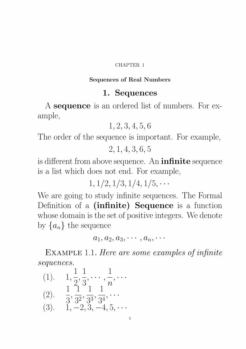
Example 1.1. Here are some examples of infinitesequences.
(1). 1,1
2,1
3, · · · ,
1
n, · · ·
(2).1
3,
1
32,
1
33,
1
34, · · ·
(3). 1,−2, 3,−4, 5, · · ·5
6 1. SEQUENCES OF REAL NUMBERS
Can you find a formula for each of the above sequences?Answer: (1). an = 1/n. (2). an = 1/3n. (3).(−1)n−1n.Historic Remarks:
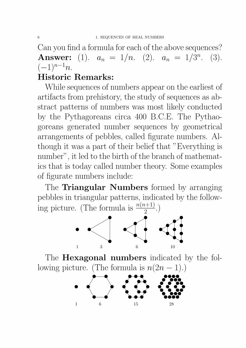
While sequences of numbers appear on the earliest ofartifacts from prehistory, the study of sequences as ab-stract patterns of numbers was most likely conductedby the Pythagoreans circa 400 B.C.E. The Pythao-goreans generated number sequences by geometricalarrangements of pebbles, called figurate numbers. Al-though it was a part of their belief that ”Everything isnumber”, it led to the birth of the branch of mathemat-ics that is today called number theory. Some examplesof figurate numbers include:
The Triangular Numbers formed by arrangingpebbles in triangular patterns, indicated by the follow-ing picture. (The formula is n(n+1)
2 .)
................................
................................
................................
................................
..................................................................................................................................................................................
................................
................................
................................
................................
. ................................
................................
................................
................................
..................................................................................................................................................................................
................................
................................
................................
................................
.
..........................................................................................................................
........
........
........
........
........
........
........
........
........
........
........
........
....
• ••
••
•••
••
•
•• •
••
•• ••
1 3 6 10
The Hexagonal numbers indicated by the fol-lowing picture. (The formula is n(2n− 1).)
...................................................................................................................................................................................................................................................................................................................................................................................................................................................... ...........................................................................................................................................................
...........................................................................................................................................................................................................................................................................................
....................................................................................................................................................
......................................................................................................................................................................................................................................................................................................................................................................................................................................................
....................................................................................................
....................................................................................................................................................................................................
•••••••
•• •••••
••
••••••
• •• •
•••
•• •
••• •••• • •
• ••
•••
•
••
1 6 15 28
2. LIMITS OF SEQUENCES 7
Links to Other Areas of Science: The topicson sequences are used in many areas of science. Forexample, much attention has been given to the se-quences that are the discrete versions of the logisticdifferential equation. The recursive equation is simpleenough, however the terms of the sequence may exhibitextremely complex behavior. This equation is used asan introduction to dynamical systems and chaos the-ory a hot area of mathematical research. The logisticdifference equation is given by
pn+1 = kpn(1− pn),
where 0 < p0 < 1 and k is a given constant. In ecology,this is a model for population growth such as modellinginsect populations, where mating and death occur in aperiodic fashion. For values of k between 3.6 and 4 thebehavior becomes chaotic.
2. Limits of Sequences
Definition 2.1. The limit of {an} is A, and iswritten as
limn→∞
an = A,
if for any ε > 0, there is a natural number N such thatfor every n > N , we have
|an − A| < ε.
Roughly speaking, limn→∞
an = A means that an be-
comes arbitrarily close to A for all sufficiently large n.
8 1. SEQUENCES OF REAL NUMBERS
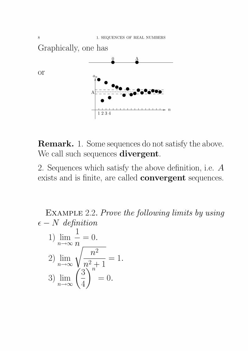
Graphically, one has
..........................................................................................................................................................................................................................................................................................................................................................................................................................................................................................................................•A•0or
............................................................................................................................................................................................................................................................................................................................................................................................................................................................................. ................
........
........
........
........
........
........
........
........
........
........
........
........
........
........
........
........
........
........
........
........
........
........
........
........
........
........
........
........
........
........
....................
................
1 2 3 4
A
n
an
........
............
........
............
........
............
........
............
........
............
........
............
........
............
........
............
........
............
•
•
•
•••••••••••••••
............. ............. ............. ............. ............. ............. ............. ............. ............. ............. ............. ............. ............. ............. ............. ............. ............
............. ............. ............. ............. ............. ............. ............. ............. ............. ............. ............. ............. ............. ............. ............. ............. ............
........................................................................................................................................................................................................................................................
Remark. 1. Some sequences do not satisfy the above.We call such sequences divergent.
2. Sequences which satisfy the above definition, i.e. Aexists and is finite, are called convergent sequences.
Example 2.2. Prove the following limits by usingε−N definition
1) limn→∞
1
n= 0.
2) limn→∞
√n2
n2 + 1= 1.
3) limn→∞
(3
4
)n
= 0.
2. LIMITS OF SEQUENCES 9
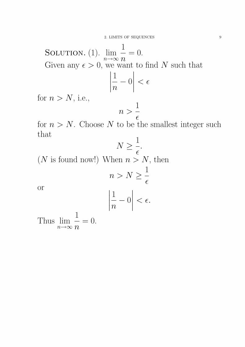
Solution. (1). limn→∞
1
n= 0.
Given any ε > 0, we want to find N such that∣∣∣∣1n − 0
∣∣∣∣ < ε
for n > N , i.e.,
n >1
εfor n > N . Choose N to be the smallest integer suchthat
N ≥ 1
ε.
(N is found now!) When n > N , then
n > N ≥ 1
εor ∣∣∣∣1n − 0
∣∣∣∣ < ε.
Thus limn→∞
1
n= 0.
10 1. SEQUENCES OF REAL NUMBERS
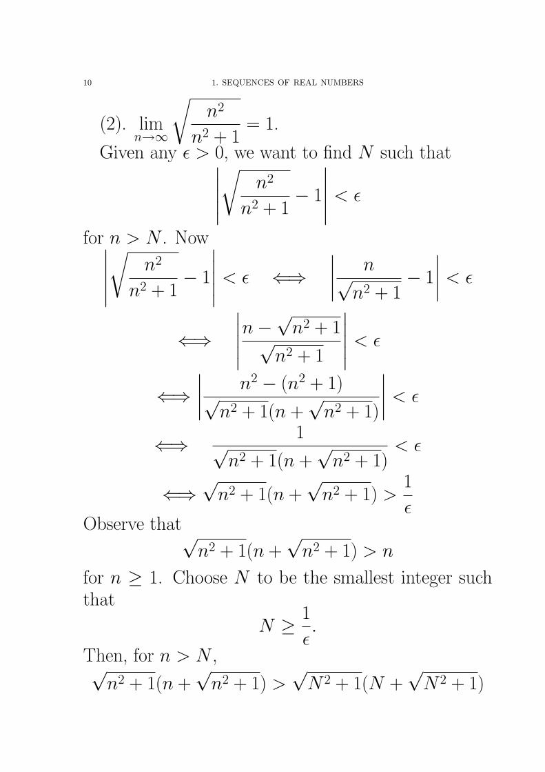
(2). limn→∞
√n2
n2 + 1= 1.
Given any ε > 0, we want to find N such that∣∣∣∣∣√
n2
n2 + 1− 1
∣∣∣∣∣ < ε
for n > N . Now∣∣∣∣∣√
n2
n2 + 1− 1
∣∣∣∣∣ < ε ⇐⇒∣∣∣∣ n√
n2 + 1− 1
∣∣∣∣ < ε
⇐⇒
∣∣∣∣∣n−√
n2 + 1√n2 + 1
∣∣∣∣∣ < ε
⇐⇒∣∣∣∣ n2 − (n2 + 1)√
n2 + 1(n +√
n2 + 1)
∣∣∣∣ < ε
⇐⇒ 1√n2 + 1(n +
√n2 + 1)
< ε
⇐⇒√
n2 + 1(n +√
n2 + 1) >1
εObserve that√
n2 + 1(n +√
n2 + 1) > n
for n ≥ 1. Choose N to be the smallest integer suchthat
N ≥ 1
ε.
Then, for n > N ,√n2 + 1(n +
√n2 + 1) >
√N 2 + 1(N +
√N 2 + 1)
2. LIMITS OF SEQUENCES 11
> N ≥ 1
εor ∣∣∣∣∣
√n2
n2 + 1− 1
∣∣∣∣∣ < ε.
Thus N is found and hence the result.
12 1. SEQUENCES OF REAL NUMBERS
(3). limn→∞
(3
4
)n
= 0.
Given any ε > 0, we want to find N such that∣∣∣∣(3
4
)n
− 0
∣∣∣∣ < ε
for n > N . Observe that(3
4
)n
< ε
⇐⇒ n ln
(3
4
)< ln(ε)
⇐⇒ n >ln(ε)
ln(3/4)(Note. ln(3/4) < 0!!) Choose N to be the smallestpositive integer such that
N ≥ ln(ε)
ln(3/4).
When n > N , then
n > N ≥ ln(ε)
ln(3/4)or∣∣∣∣(3
4
)n
− 0
∣∣∣∣ < ε.
The proof is finished. �
2. LIMITS OF SEQUENCES 13
Remark. In the above proofs, we have used thefollowing basic property of real numbers:
Archimedean Property: For any given real num-ber x, there exists a natural number N (depending onx) such that N > x.
Theorem 2.3. If {an} has a limit, then the limitis unique.
Proof. Let A and B be limits of {an}. Suppose
that A 6= B. Choose ε =|A−B|
2.
Then ε > 0 because A 6= B. By definition, thereexists N1 and N2 such that
|an − A| < ε
for n > N1 and|an −B| < ε
for n > N2.For n > max{N1, N2}, we have
|A−B| = |(A−an)+(an−B)| ≤ |A−an|+ |an−B|
< 2ε = 2|A−B|
2= |A−B|,
which is a contradiction. Thus A = B. �
14 1. SEQUENCES OF REAL NUMBERS
Theorem 2.4 (Squeeze or Sandwich Theorem). Giventhree sequences
{an}, {bn}, {cn}such that
(i) an ≤ bn ≤ cn for every n and
(ii) limn→∞
an = A = limn→∞
cn,
then limn→∞
bn = A.
Remark. The above theorem is still applicable if theinequality
an ≤ bn ≤ cn
is true eventually.
2. LIMITS OF SEQUENCES 15
Proof. For any ε > 0, there exists N1 and N2 suchthat
|cn − A| < ε
for n > N1 and|an − A| < ε
for n > N2. Let N = max{N1, N2}. For n > N , wehave
−ε < cn − A < ε and − ε < an − A < ε
A− ε < cn < A + ε and A− ε < an < A + ε.
Thus
A− ε < an ≤ bn ≤ cn < A + ε or |bn − A| < ε.
By definition, we have limn→∞
bn = A and hence the
result. �
16 1. SEQUENCES OF REAL NUMBERS
Example 2.5. Find limits
1) limn→∞
1 + sin n
n.
2)
(3n− 1
4n + 1
)n
.
Solution. (1). Since
0 ≤ 1 + sin n
n≤ 2
n
and limn→∞
2
n= lim
n→∞0 = 0, we have
limn→∞
1 + sin n
n= 0.
(2). Since
0 ≤(
3n− 1
4n + 1
)n
≤(
3
4
)n
and limn→∞
(3
4
)n
= limn→∞
0 = 0, we have
limn→∞
(3n− 1
4n + 1
)n
= 0.
�
3. SEQUENCES WHICH TEND TO ∞ 17
3. Sequences which tend to ∞Definition 3.1. {an} tends to +∞ if for each
number k, there is an N such that
an > k for all n > N.
Remark. For such sequences, we write as an → +∞as n →∞ or
limn→∞
an = +∞.
{an} tends to −∞ if for each number k, there is anN such that
an < k for all n > N.
In this case, write limn→∞
an = −∞.
Example 3.2. The following sequences tend to +∞1) an =
√ln n.
2) an = (3/2)n.
The sequences − ln n, −n2 and etc then tend to −∞.
18 1. SEQUENCES OF REAL NUMBERS
Theorem 3.3 (Reciprocal Rule). Consider a se-quence {an}.
(i) If an > 0 for all n and limn→∞
1
an= 0, then
limn→∞
an = +∞.
(ii) If limn→∞
an = ±∞, then limn→∞
1
an= 0.
Proof. We only prove (i). For each positive integerk, there exists N such that∣∣∣∣ 1
an− 0
∣∣∣∣ < 1
k
for n > N because limn→∞
1
an= 0. Then, for n > N ,
an > k because an > 0. This finishes the proof. �
Example 3.4. Since limn→∞
1√n
= 0, we have limn→∞
√n =
∞. Similarly, since limn→∞
√n = +∞, we have lim
n→∞
1√n
=
0.
4. TECHNIQUES FOR COMPUTING LIMITS 19
4. Techniques For Computing Limits
Theorem 4.1. Let f be a continuous function.Then
limn→∞
f (an) = f ( limn→∞
an).
Idea of Proof. By the definition of continuity,when x → x0, f (x) → f (x0). Now lim
n→∞an = A
means that an → A when n → ∞. Thus f (an) →f (A) when n →∞, that is,
limn→∞
f (an) = f (A) = f ( limn→∞
an).
�
Example 4.2.
limn→∞
sin
(nπ
2n + 1
)= lim
n→∞
(π
2 + 1/n
)= sin
(π
2
)= 1.
20 1. SEQUENCES OF REAL NUMBERS
Theorem 4.3 (L’Hospital’s Rule). Suppose an =f (n), bn = g(n) for differentiable functions f and
g. If limn→∞
f (n)
g(n)is of the form
∞∞
or0
0, then
limn→∞
f (n)
g(n)= lim
n→∞
f ′(n)
g′(n).
History Remark. Although the theorem is namedafter Marquis de l’Hospital (1661-1704), it should becalled Bernoulli’s rule. The story is that in 1691, l’Hospitalasked Johann Bernoulli (1667-1748) to provide, for afee, lectures on the new subject of calculus. L’Hospitalsubsequently incorporated these lectures into the firstcalculus text, L’Analyse des infiniment petis (Anal-ysis of infinitely small quantities), published in 1696.The initial version of what is now known as l’Hospital’srule first appeared in this text.
Example 4.4. Show that limn→∞
(1 +
x
n
)n
= ex.
Proof.
limn→∞
ln[(
1 +x
n
)n]= lim
n→∞n ln
(1 +
x
n
)= lim
n→∞
ln(1 + x
n
)1/n
= limn→∞
11+x
n·(− x
n2
)− 1
n2
= limn→∞
x
1 + xn
= x.
Thus limn→∞
(1 +
x
n
)n
= ex. �
4. TECHNIQUES FOR COMPUTING LIMITS 21
Theorem 4.5. If limn→∞
an and limn→∞
bn exist, then
(1). {an+bn} converges with limn→∞
(an+bn) = limn→∞
an+
limn→∞
bn;
(2). {an−bn} converges with limn→∞
(an−bn) = limn→∞
an−lim
n→∞bn;
(3). {kan} converges with limn→∞
kan = k limn→∞
an, where
k is a fixed constant;(4). {anbn} converges with lim
n→∞anbn = lim
n→∞an lim
n→∞bn;
(5).
{an
bn
}converges with lim
n→∞
an
bn=
limn→∞
an
limn→∞
bn, pro-
vided bn 6= 0 and limn→∞
bn 6= 0.
Proof. See Bartle-Sherbert [1, page 60-61]. �
Example 4.6. Find the limit of
ln
(n2 + 3n + 2
2 + 4n + 2n2
)+ cos
(1√n
).
22 1. SEQUENCES OF REAL NUMBERS
Solution.
limn→∞
[ln
(n2 + 3n + 2
2 + 4n + 2n2
)+ cos
(1√n
)]= lim
n→∞
[ln
((n2 + 3n + 2)/n2
(2 + 4n + 2n2)/n2
)+ cos
(1√n
)]= lim
n→∞
[ln
(1 + 3/n + 2/n2
2/n2 + 4/n + 2
)+ cos
(1√n
)]= ln
(1 + 0 + 0
0 + 0 + 2
)+ cos 0 = ln
(1
2
)+ 1 = 1− ln 2.
�
4. TECHNIQUES FOR COMPUTING LIMITS 23
Theorem 4.7 (Some Standard Limits). Some stan-dard limits are given as follows.
1. limn→∞
1
np= 0 for any fixed p > 0.
2. limn→∞
cn = 0 for any fixed c where |c| < 1.
3. limn→∞
c1n = 1 for any fixed c > 0.
4. limn→∞
n√
n = 1.
5. limn→∞
np
cn= 0 for any fixed p and c > 1.
6. limn→∞
cn
n!= 0 for any fixed c.
7. limn→∞
(1 +
x
n
)n
= ex for any fixed x.
8. limn→∞
(ln n)p
nk= 0 for any fixed k > 0.
24 1. SEQUENCES OF REAL NUMBERS
Proof. 1. limn→∞
1
np= 0 for any fixed p > 0.
limn→∞
1
np=(
limn→∞
1
n
)p
= 0p = 0.
2. limn→∞
cn = 0 for any fixed c where |c| < 1.
Case 1: When c = 0, the statement is obvious.
Case 2: When c > 0, we have
ln(
limn→∞
cn)
= limn→∞
ln cn = limn→∞
n ln c = −∞.
Thus, limn→∞
cn = 0.
Case 3: When c < 0, we have −|c|n ≤ cn ≤ |c|n forall n. By Case 2, we have lim
n→∞(−|c|n) = 0 = lim
n→∞|c|n.
Hence by Squeeze theorem, we also have limn→∞
cn = 0.
3. limn→∞
c1n = 1 for any fixed c > 0.
limn→∞
c1n = c
limn→∞
1n = c0 = 1.
4. TECHNIQUES FOR COMPUTING LIMITS 25
4. limn→∞
n√
n = 1.
ln(
limn→∞
n√
n)
= limn→∞
ln n√
n
= limn→∞
ln n
n= 0 (by L’Hospital’s rule).
Thus, limn→∞
n√
n = e0 = 1.
5. limn→∞
np
cn= 0 for any fixed p and c > 1.
Let k be a fixed positive integer such that p−k < 0.Then
limn→∞
np
cn= lim
n→∞
pnp−1
cn ln c= lim
p(p− 1)np−2
cn(ln c)2= · · ·
= limn→∞
p(p− 1) · · · (p− k + 1)np−k
cn(ln c)k
= limn→∞
p(p− 1) · · · (p− k + 1)
cnnk−p(ln c)k= 0
by L’Hospital’s rule.
26 1. SEQUENCES OF REAL NUMBERS
6. limn→∞
cn
n!= 0 for any fixed c.
Let an =cn
n!=
c · c · · · · · cn(n− 1) · · · · · 1
. Now fix an integer
M > c. Then for any n > M ,
0 < an =c · c · · · · · c
n(n− 1) · · · · · (M + 1)aM <
c
naM .
Note that aM is a fixed number because M is fixed.
Since limn→∞
0 = 0 = limn→∞
c
naM , by the Squeeze theorem,
limn→∞
an = 0.
7. limn→∞
(1 +
x
n
)n
= ex for any fixed x. It was proved
in Example 4.4.
8. limn→∞
(ln n)p
nk= 0 for any fixed k > 0.
Let m = ln n. Then n = em. By (5),
limn→∞
(ln n)p
nk= lim
m→∞
mp
ekm= lim
m→∞
mp
(ek)m = 0,
where ek > 1 because k > 0. �
4. TECHNIQUES FOR COMPUTING LIMITS 27
Strategy: One can find the limits of many sequencesfrom those of the standard sequences.
Example 4.8. Find the limits
1) limn→∞
8n + (ln n)10 + n!
n6 − n!.
2) limn→∞
(1− 1
2n + 1
)3n
.
Solution. (1).
limn→∞
8n + (ln n)10 + n!
n6 − n!= lim
n→∞
8n/n! + (ln n)10/n! + 1
n6/n!− 1
=0 + 0 + 1
0− 1= −1.
(2).
limn→∞
(1− 1
2n + 1
)3n
= limn→∞
[(1 +
−1
2n + 1
)2n+1] 3n
2n+1
= limn→∞
[(1 +
−1
2n + 1
)2n+1] 3
2+1/n
=(e−1)3
2 =1
e√
e
�
28 1. SEQUENCES OF REAL NUMBERS
5. The Least Upper Bounds and theCompleteness Property of R
5.1. From Natural Numbers to Real Num-bers. Starting with natural numbers N = {1, 2, 3, · · · },we obtain real numbers R by adding more and morenew numbers in the following steps:
Step 1. By adding 0 and negative numbers, we haveintegers Z = {0,±1,±2,±3, · · · }.Step 2. Then we have rational numbers
Q =
{p
q
∣∣∣ p, q ∈ Z, q 6= 0
}.
Step 3. Then, by adding irrational numbers, wehave all real numbers.
Below we give some examples of irrational num-bers. Recall that a natural number p > 1 is calledprime if p is NOT divisible by any natural numbersother than p and 1. For instance, 2, 3, 5, 7, 11, · · · areprimes. Every natural number n > 1 admits a unique(prime) factorization
n = p1 · p2 · · · pk,
where each pi is prime. For instance, 20 = 2 · 2 · 5 and66 = 2 · 3 · 11.
5. THE LEAST UPPER BOUNDS AND THE COMPLETENESS PROPERTY OF R 29
Example 5.1. If n is a natural number, and thereis no natural number whose square is n, then
√n is
NOT a rational number. In particular,√
2,√
3,√
5,√
6are irrational numbers.
Proof. Suppose that√
n is a rational number. We
can write√
n asa
b, where a, b ∈ N and b 6= 0. Then
√n =
a
b⇐⇒ n =
a2
b2⇐⇒ a2 = b2n.
Any prime occurring in the (unique) factorization of awill occur an even number of times in the factorizationof a2; similarly for b and b2.
By a2 = b2n, any prime that occurs in the factoriza-tion of n must occur an even number of times, since allprimes occurring in the factorization of b2n are exactlythose occurring in the factorization of a2.
Thus n can be written as
n = (p1 · p2 · · · pk)2,
where, of course, the pi’s need not be distinct.
This, however, is a contradiction to the hypothesis,since n is expressed as the square of a natural number.
�
30 1. SEQUENCES OF REAL NUMBERS
5.2. Bounded Sets.
Definition 5.2. A set of real numbers S is boundedabove if there exists a finite real number M such that
x ≤ M ∀x ∈ S.
M is called an upper bound of S.
Definition 5.3. A set of real numbers S is boundedbelow if there exists a finite real number m such that
m ≤ x ∀x ∈ S.
m is called a lower bound of S.
Definition 5.4. A set which is both bounded aboveand below is called a bounded set.
Remark.1. Upper bounds and lower bounds are not unique.
2. Some sets only have upper bounds but not lowerbounds.
3. Some sets have only lower bounds but not upperbounds.
4. A set which is not bounded is called an unboundedset.
Example 5.5. Let
S = {r | r is a rational number with r <√
2}.Then S is bounded above.
5. THE LEAST UPPER BOUNDS AND THE COMPLETENESS PROPERTY OF R 31
Theorem 5.6. Every convergent sequence isbounded.
Proof. Let {an} be a sequence convergent to A.For ε = 1, there exists N such that |an − A| < 1 orA− 1 < an < A + 1 for n > N .
Choose M and m to be the largest and smallestnumber of the finite numbers
a1, a2, . . . , aN , A + 1, A− 1,
respectively.
When n ≤ N , we have m ≤ an ≤ M because M(m) is the largest (smallest) number of the above finiteset. When n > N , we have
m ≤ A− 1 < an < A + 1 ≤ M.
Thus, for all n, we have m ≤ an ≤ M and so {an} isbounded. The proof is finished. �
Corollary 5.7 (Test for divergence). If {an} isunbounded, then {an} diverges.
32 1. SEQUENCES OF REAL NUMBERS
Remark.1. The converse may not be true, i.e., divergent se-quence need not be unbounded.
2. The inverse may not be true, i.e., a bounded se-quence may not be convergent.
Example. The sequence {1,−1, 1,−1, · · · } is boundedbut NOT convergent.
5. THE LEAST UPPER BOUNDS AND THE COMPLETENESS PROPERTY OF R 33
5.3. Infimum and Supremum. Recall that anyfinite set of real numbers has a greatest element (max-imum) and a least element (minimum).
Example 5.8. {−2.5, 3.1, −4.4, 4.5, 5}
However, this property does not necessarily hold forinfinite sets.
Example 5.9. {1, 2, 3, 4, · · · , }.
Definition 5.10. A real number M ( 6= ±∞) iscalled the least upper bound or supremum of aset E if
(S-i) M is an upper bound of E, i.e., x ≤ M forevery x ∈ E, and
(S-ii) if M ′ < M , then M ′ is not an upper bound ofE (i.e., there is an x ∈ E such that M ′ < x).
We write M = sup E.
34 1. SEQUENCES OF REAL NUMBERS
Remark.(i) sup E is unique whenever it exists.
(ii) The main difference between sup E and max Eis that sup E need not be an element of E, whereasmax E must be an element of E if it does exist).
(iii) If E has a maximum, then sup E = max E.
Example 5.11. 1. Let E = {r ∈ Q | 0 ≤ r ≤√
2}.Then sup E =
√2 but max E does not exist because√
2 is not a rational number, that is, sup E 6∈ E.
2. Let E = {1/2, 2/3, 3/4, 4/5, 5/6, · · · }. Then sup E =1 and max E does not exist.
3. Let E = {1, 1/2, 1/3, 1/4, 1/5, · · · }. Then max E =1 = sup E.
5. THE LEAST UPPER BOUNDS AND THE COMPLETENESS PROPERTY OF R 35
Definition 5.12. A real number m ( 6= ±∞) iscalled the greatest lower bound or infimum of aset E if
(i) m is a lower bound of E, i.e., m ≤ x for everyx ∈ E, and
(ii) if m′ > m, then m′ is not a lower bound of E(i.e., there exists an x ∈ E such that x < m′).
We write m = inf E.
Remark.(i) inf E is unique whenever it exists.
(ii) The main difference between inf E and min E isthat inf E need not be an element of E, whereasmin E must be an element of E if it does exist.
(iii) If E has a minimum, then inf E = min E.
Example 5.13. 1. Let E = {1, 1/2, 1/3, 1/4, · · · , }.Then inf E = 0 but min E does not exist.
2. Let E = {r ∈ Q | 0 ≤ r ≤√
2}. Then min E =inf E = 0.
36 1. SEQUENCES OF REAL NUMBERS
5.4. The Completeness of R. A very basic butimportant property of the set of real numbers is thefollowing:
Theorem 5.14 (Completeness Axiom of R). Thefollowing statement hold for subsets of real num-bers:
(i) If E is bounded above, then sup E exists.
(ii) If E is bounded below, then inf E exists.
Recall that a set E is bounded if and only if it isbounded above and bounded below. Thus the Com-pleteness Axiom leads to
Corollary 5.15. If E is bounded, then bothsup E and inf E exist.
To see this, we will need an important property ofrational numbers:
Theorem 5.16 (Density Theorem of Q). For anytwo real numbers x, y ∈ R satisfying x < y, thereexist a rational number r ∈ Q such that
x < r < y.
..........................................................................................................................................................................................................................................................................................................................................................................................................................................................................................................................•0
5. THE LEAST UPPER BOUNDS AND THE COMPLETENESS PROPERTY OF R 37
Proof. Since y > x, we have y − x > 0 and thus1
y − x∈ R (and
1
y − x> 0).
Then by the Archimedean Property of R, there exista natural number n ∈ N such that
n >1
y − x=⇒ ny − nx > 1 =⇒ ny > 1 + nx,
noting that y − x > 0. Then the smallest integer msatisfying m > nx must also satisfy m ≤ nx+1 < ny.Thus, we have
nx < m < ny =⇒ x <m
n< y,
where r = m/n is rational. �
Example 5.17. Let E = {x ∈ Q : x2 < 3}. Thensup E =
√3.
Proof. For any x ∈ E, we have
x2 < 3 =⇒ x <√
3
upon taking positive square roots on both sides. Thus,E is bounded above (by
√3. Also, it is easy to see that
E 6= ∅ (for example, 0 ∈ E). Thus by the Complete-ness Axiom of R, sup E exists in R. Since
√3 is an
upper bound for E, it follows from that√
3 ≥ sup E.Suppose
√3 6= sup E. Then we must have
√3 >
sup E. But by the Density Theorem for Q, there existsa rational number r ∈ Q such that
sup E < r <√
3.
38 1. SEQUENCES OF REAL NUMBERS
Then r ∈ Q and r2 < 3. Hence we have r ∈ Eand r ≤ sup E, which contradicts to that sup E < r.Hence we must have
√3 = sup E. �
Remark. The above example shows that sup E maybe in R but NOT in Q, even though E ⊂ Q. In otherwords, the Completeness Axiom does not hold for theset of rational numbers Q.
We will also adopt the following convention:
Definition 5.18. (i) If ∅ 6= E ⊂ R is not boundedabove, then we write sup E = +∞.(i) If ∅ 6= E ⊂ R is not bounded below, then wewrite inf E = −∞.
6. MONOTONE SEQUENCES 39
6. Monotone Sequences
Definition 6.1. {an} is called monotone in-creasing (decreasing) if
an ≤ (≥) an+1
for every n, that is,
a1 ≤ a2 ≤ a3 ≤ a4 ≤ · · ·(a1 ≥ a2 ≥ a3 ≥ · · · ).
Example 6.2. (1). The sequence {1/n} is mono-tone decreasing.
(2). The sequence {1/2, 2/3, 3/4, 4/5, 5/6, · · · } is mono-tone increasing.
Proposition 6.3. A monotone increasing (de-creasing) sequence is bounded below (above).
Proof. Let {an} be a monotone increasing sequence,that is,
a1 ≤ a2 ≤ a3 ≤ · · · .
Then a1 is a lower bound for {an} and hence the result.�
40 1. SEQUENCES OF REAL NUMBERS
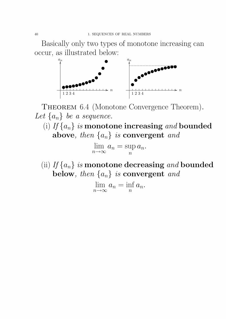
Basically only two types of monotone increasing canoccur, as illustrated below:
................................................................................................................................................................................................................................................................................................................................................................. ................
........
........
........
........
........
........
........
........
........
........
........
........
........
........
........
........
........
........
........
........
........
........
........
........
........
........
........
........
........
........
....................
................
1 2 3 4n
an
........
............
........
............
........
............
........
............
........
............
........
............
........
............••••••••
••••••
................................................................................................................................................................................................................................................................................................................................................................. ................
........
........
........
........
........
........
........
........
........
........
........
........
........
........
........
........
........
........
........
........
........
........
........
........
........
........
........
........
........
........
....................
................
1 2 3 4n
an
........
............
........
............
........
............
........
............
........
............
........
............
........
............
••••••
••••••••...............................................................................................................................................................................................
Theorem 6.4 (Monotone Convergence Theorem).Let {an} be a sequence.
(i) If {an} is monotone increasing and boundedabove, then {an} is convergent and
limn→∞
an = supn
an.
(ii) If {an} is monotone decreasing and boundedbelow, then {an} is convergent and
limn→∞
an = infn
an.
6. MONOTONE SEQUENCES 41
Proof. (i). Suppose {an} is monotone increasingand bounded above.
Then by the Completeness Axiom of R, supn
an exists
(finite).
Now, given ε > 0, since supn
an − ε < supn
an, it
follows that supn
an− ε is not an upper bound of {an}.In other words, there exists an integer N such that
aN > supn
an − ε. Then for all n > N , we have
supn
an−ε < aN ≤ an ≤ supn
an < supn
an+ε (since n > N).
Equivalently,
∣∣∣∣an − supn
an
∣∣∣∣ < ε for all n > N and
so limn→∞
an = supn
an (exists).
The proof of (ii) is similar. �
42 1. SEQUENCES OF REAL NUMBERS
Example 6.5. Let an =n
n + 1, that is,
{an} = {1/2, 2/3, 3/4, · · · }.Then an is monotone increasing and bounded above.Thus
supn
an = limn→∞
an = 1.
Corollary 6.6. If {an} is monotone increasing(decreasing), then either
(i) {an} is convergent or(ii) lim
n→∞an = +∞(−∞).
6. MONOTONE SEQUENCES 43
Proof. Suppose {an} is monotone increasing, theneither {an} is bounded above or not bounded above.
Case (a): If {an} is bounded above, then by theMonotone Convergence Theorem, {an} converges.
Case (b): If {an} is not bounded above, then {an}has no upper bounds. Thus for any given k > 0, kis not an upper bound of {an}. In other words, thereexists N such that
aN > k.
Since {an} is monotone increasing, it follows that forall n > N ,
an ≥ aN > k.
Therefore, limn→∞
an = +∞.
The proof for the case when {an} is monotone de-creasing is similar. �

44 1. SEQUENCES OF REAL NUMBERS
7. Subsequences
Example 7.1. The following are the subsequencesof {an} = {1,−1, 1,−1, 1,−1, · · · }.{a2n−1} = {1, 1, 1, · · · }{a2n} = {−1,−1,−1, · · · }.
In general, subsequences of {an} are of the form{ank
}, k = 1, 2, 3, ..., with
n1 < n2 < n3 < · · · .
Note. The rule is that we should choose an1 first andthen an2 with n2 > n1 and then an3 with n3 > n2, sofar and so on (up to infinite). Thus n1 is at least 1, n2
is at least 2, n3 is at least 3, · · · .
7. SUBSEQUENCES 45
Theorem 7.2. Suppose limn→∞
an = A. Then ev-
ery subsequence of {an} also converges to A,that is,
limk→∞
ank= A.
Proof. For any given ε > 0, since limn→∞
an = A,
there exists N such that
|an − A| < ε for all n > N.
Then for all k > N , we have
nk ≥ k > N.
Hence|ank
− A| < ε for all k > N.
Therefore, limk→∞
ank= A. �
46 1. SEQUENCES OF REAL NUMBERS
Corollary 7.3. Suppose that {an} has two sub-sequences that converge to different limits.Then {an} is divergent. �
Example 7.4. The sequence {1,−1, 1,−1, · · · } isdivergent because {a2n−1} = {1, 1, · · · } converges to1 and {a2n} = {−1,−1, · · · } converges to −1.
8. THE LIMIT SUPERIOR AND INFERIOR OF A SEQUENCE 47
8. The Limit Superior and Inferior of aSequence
Given a sequence {an}, we can form another se-quence {bn} given by
bn = supk≥n
ak = sup{an, an+1, an+2, · · · }.
Example 8.1. Let {an} = {1,−1, 1,−1, · · · }. Then
bn = supk≥n
ak = sup{±1,∓1,±1,∓1, · · · } = 1.
Proposition 8.2. For any sequence {an}, theassociated sequence {bn} = {sup
k≥nak} is always
monotone decreasing.
Proof. For each n,
bn = sup{an, an+1, an+2, · · · }≥ sup{an+1, an+2, · · · } = bn+1.
�
Definition 8.3. The limit superior of {an}, de-noted by lim sup an or lim sup
n→∞an or lim
n→∞an is defined
to be limn→∞
bn, i.e.
limn→∞
an = limn→∞
bn = limn→∞
supk≥n
ak.
48 1. SEQUENCES OF REAL NUMBERS
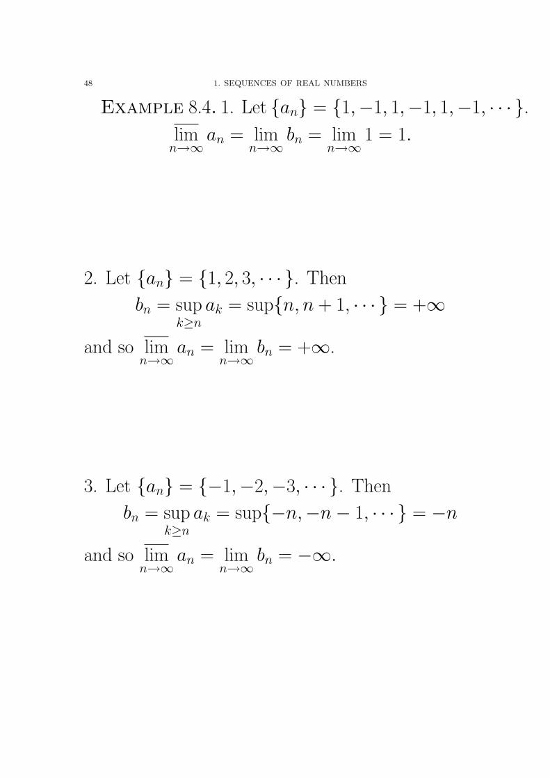
Example 8.4. 1. Let {an} = {1,−1, 1,−1, 1,−1, · · · }.lim
n→∞an = lim
n→∞bn = lim
n→∞1 = 1.
2. Let {an} = {1, 2, 3, · · · }. Then
bn = supk≥n
ak = sup{n, n + 1, · · · } = +∞
and so limn→∞
an = limn→∞
bn = +∞.
3. Let {an} = {−1,−2,−3, · · · }. Then
bn = supk≥n
ak = sup{−n,−n− 1, · · · } = −n
and so limn→∞
an = limn→∞
bn = −∞.

8. THE LIMIT SUPERIOR AND INFERIOR OF A SEQUENCE 49
Theorem 8.5. Given any sequence {an}, either
(1). limn→∞
an exists (finite), or
(2). limn→∞
an = +∞, or
(3). limn→∞
an = −∞.
Proof. If {an} is not bounded above, then each bn
is +∞, and thus
limn→∞
an = limn→∞
bn = +∞.
If {an} is bounded above, then each bn is finite. Since{bn} is monotone decreasing, by Corollary 1.6.6, {an}converges (to a finite limit), or lim
n→∞bn = −∞. �
50 1. SEQUENCES OF REAL NUMBERS
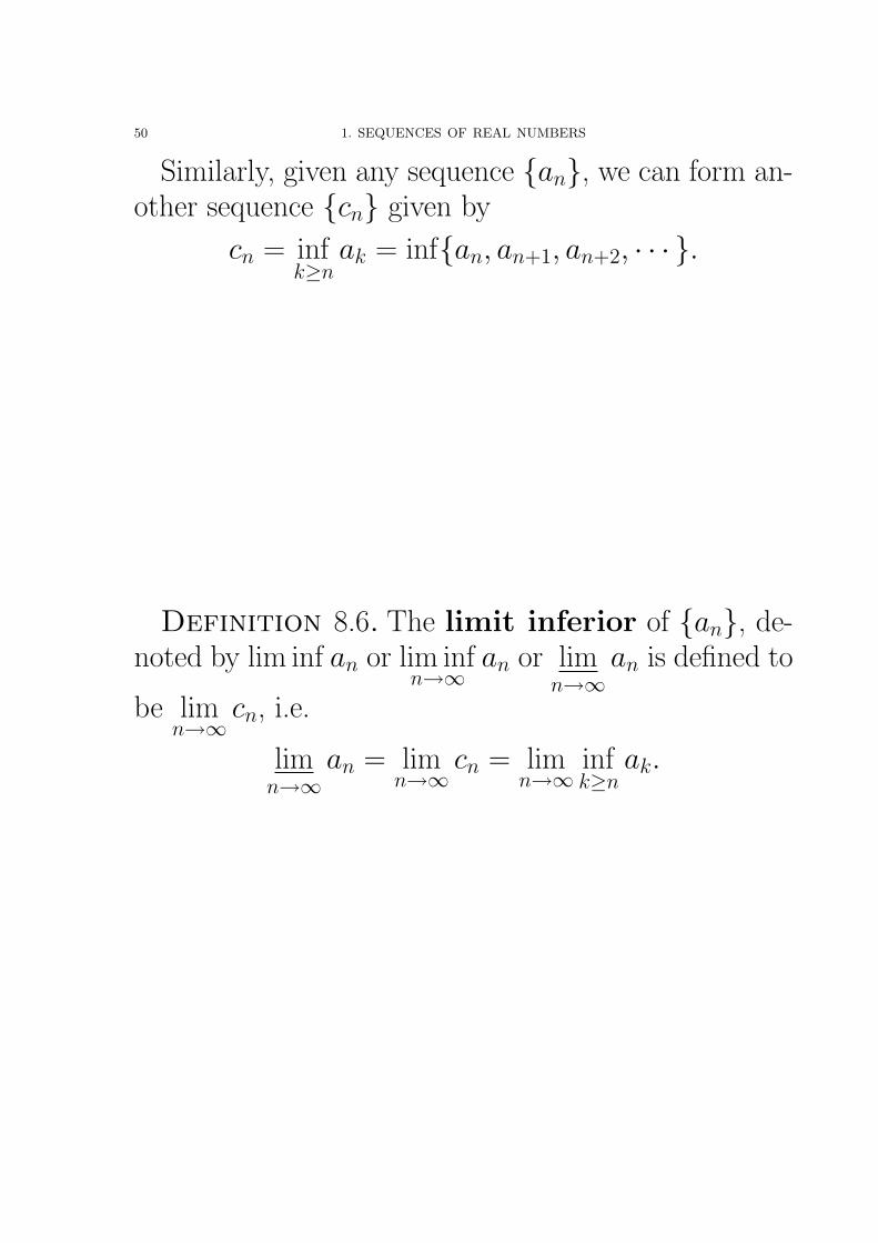
Similarly, given any sequence {an}, we can form an-other sequence {cn} given by
cn = infk≥n
ak = inf{an, an+1, an+2, · · · }.
Definition 8.6. The limit inferior of {an}, de-noted by lim inf an or lim inf
n→∞an or lim
n→∞an is defined to
be limn→∞
cn, i.e.
limn→∞
an = limn→∞
cn = limn→∞
infk≥n
ak.
8. THE LIMIT SUPERIOR AND INFERIOR OF A SEQUENCE 51
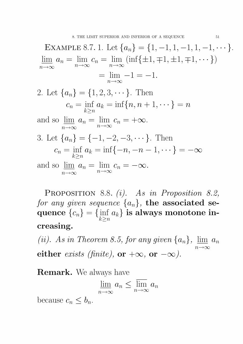
Example 8.7. 1. Let {an} = {1,−1, 1,−1, 1,−1, · · · }.lim
n→∞an = lim
n→∞cn = lim
n→∞(inf{±1,∓1,±1,∓1, · · · })
= limn→∞
−1 = −1.
2. Let {an} = {1, 2, 3, · · · }. Then
cn = infk≥n
ak = inf{n, n + 1, · · · } = n
and so limn→∞
an = limn→∞
cn = +∞.
3. Let {an} = {−1,−2,−3, · · · }. Then
cn = infk≥n
ak = inf{−n,−n− 1, · · · } = −∞
and so limn→∞
an = limn→∞
cn = −∞.
Proposition 8.8. (i). As in Proposition 8.2,for any given sequence {an}, the associated se-quence {cn} = { inf
k≥nak} is always monotone in-
creasing.
(ii). As in Theorem 8.5, for any given {an}, limn→∞
an
either exists (finite), or +∞, or −∞).
Remark. We always have
limn→∞
an ≤ limn→∞
an
because cn ≤ bn.
52 1. SEQUENCES OF REAL NUMBERS
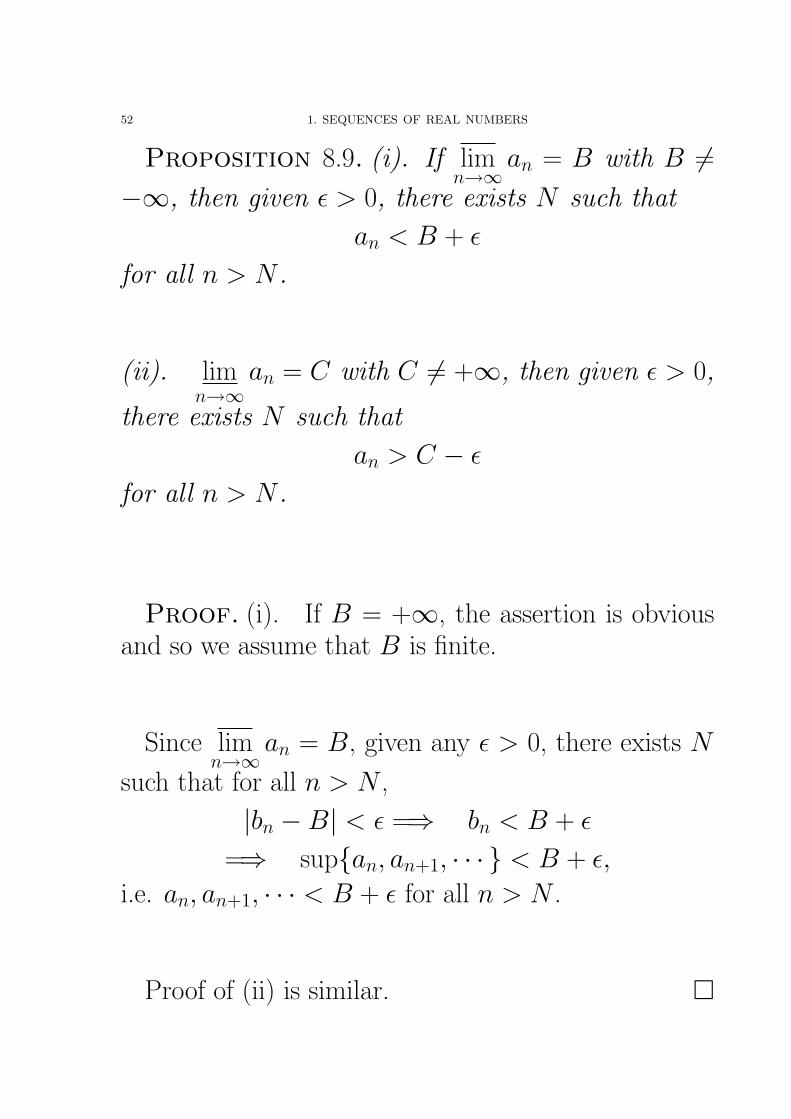
Proposition 8.9. (i). If limn→∞
an = B with B 6=−∞, then given ε > 0, there exists N such that
an < B + ε
for all n > N .
(ii). limn→∞
an = C with C 6= +∞, then given ε > 0,
there exists N such that
an > C − ε
for all n > N .
Proof. (i). If B = +∞, the assertion is obviousand so we assume that B is finite.
Since limn→∞
an = B, given any ε > 0, there exists N
such that for all n > N ,
|bn −B| < ε =⇒ bn < B + ε
=⇒ sup{an, an+1, · · · } < B + ε,
i.e. an, an+1, · · · < B + ε for all n > N .
Proof of (ii) is similar. �
8. THE LIMIT SUPERIOR AND INFERIOR OF A SEQUENCE 53
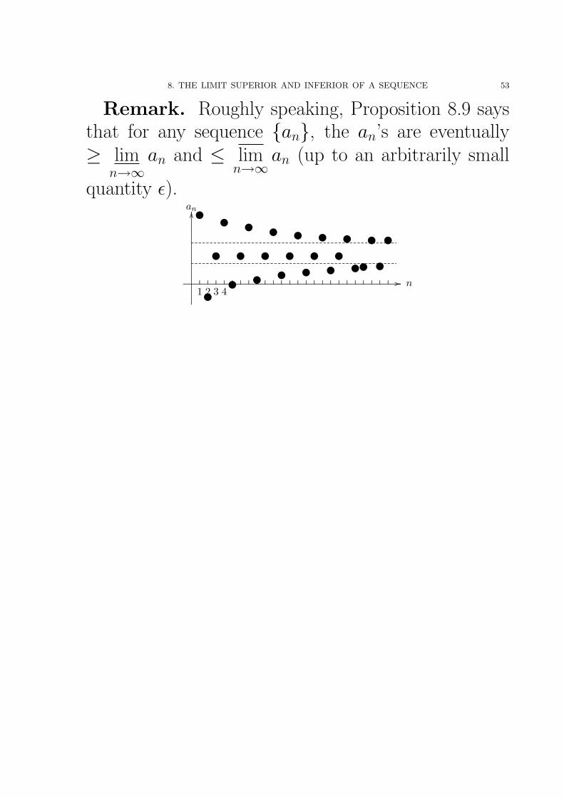
Remark. Roughly speaking, Proposition 8.9 saysthat for any sequence {an}, the an’s are eventually≥ lim
n→∞an and ≤ lim
n→∞an (up to an arbitrarily small
quantity ε).
............................................................................................................................................................................................................................................................................................................................................................................................................................................................................................................................................................................................................... ................
........
........
........
........
........
........
........
........
........
........
........
........
........
........
........
........
........
........
........
........
........
........
........
........
........
........
........
........
........
........
....................
................
1 2 3 4n
an
........
............
........
............
........
............
........
............
........
............
........
............
........
............
........
............
........
............
........
............
........
............
........
............
•
•
••
•••
•••
•••
•••••••••••.......................................................................................................................................................................................................................................................................................................................................
.......................................................................................................................................................................................................................................................................................................................................
54 1. SEQUENCES OF REAL NUMBERS
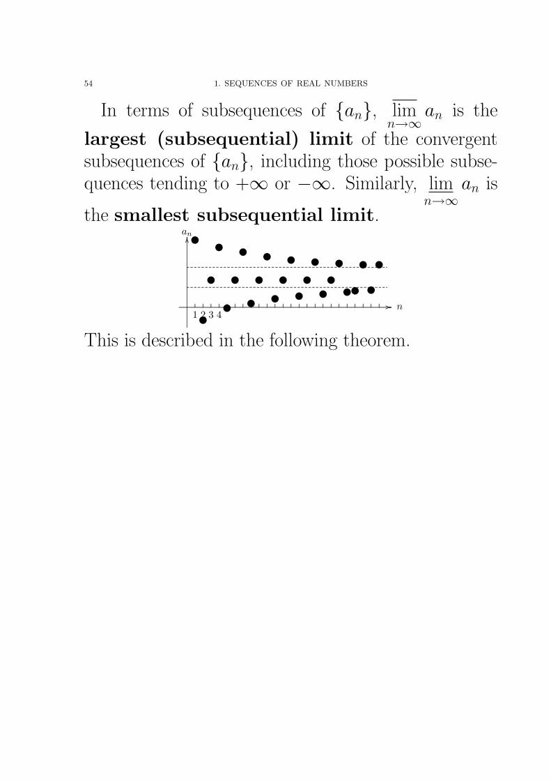
In terms of subsequences of {an}, limn→∞
an is the
largest (subsequential) limit of the convergentsubsequences of {an}, including those possible subse-quences tending to +∞ or −∞. Similarly, lim
n→∞an is
the smallest subsequential limit.
............................................................................................................................................................................................................................................................................................................................................................................................................................................................................................................................................................................................................... ................
........
........
........
........
........
........
........
........
........
........
........
........
........
........
........
........
........
........
........
........
........
........
........
........
........
........
........
........
........
........
....................
................
1 2 3 4n
an
........
............
........
............
........
............
........
............
........
............
........
............
........
............
........
............
........
............
........
............
........
............
........
............
•
•
••
•••
•••
•••
•••••••••••.......................................................................................................................................................................................................................................................................................................................................
.......................................................................................................................................................................................................................................................................................................................................
This is described in the following theorem.
8. THE LIMIT SUPERIOR AND INFERIOR OF A SEQUENCE 55
Theorem 8.10. Let {an} be any sequence. LetB = lim
n→∞an and let C = lim
n→∞an.
(i) Let {ank} be any subsequence of {an} such
that limk→∞
ankexists, +∞, or −∞. Then
C = limn→∞
an ≤ limk→∞
ank≤ lim
n→∞an = B.
(ii) There exists a subsequence {ank} of {an}
such that
limk→∞
ank= B.
(iii) There exists a subsequence {amk} of {an}
such that
limk→∞
amk= C.
56 1. SEQUENCES OF REAL NUMBERS
Proof. The proof is omitted. See the packed lec-ture notes.
�
Example 8.11. Find the limit inferior and limitsuperior of the following sequences
i)
{1− 2(−1)nn
3n + 2
},
ii){
(1 + (−1)n) sinnπ
4
},
iii) {[1.5 + (−1)n]n} .
Solution. (i). Note that
a2k =1− 2 · 2k3 · 2k + 2
limk→∞
a2k = limk→∞
1/k − 4
6 + 2/k= −4
6= −2
3
a2k−1 =1 + 2 · (2k − 1)
3 · (2k − 1) + 2
limk→∞
a2k−1 = limk→∞
1/k + 2 · (2− 1/k)
3 · (2− 1/k) + 2/k=
4
6=
2
3
Thus the subsequential limits are ±2
3and so
limn→∞
an =2
3and lim
n→∞an = −2
3.
8. THE LIMIT SUPERIOR AND INFERIOR OF A SEQUENCE 57
(ii). The sequence{(1 + (−1)n) sin
nπ
4
}=
{0, 2 sin
2π
4= 2, 0, 2 sin
4π
4= 0, 0, 2 sin
6π
4= −2,
0, 2 sin8π
4= 0, 0, 2 sin
10π
4= 2, · · ·
}.
The subsequential limits are −2, 0 and 2. Thus
limn→∞
an = 2 and limn→∞
an = −2.
(iii). {[1.5 + (−1)n]n} .Note that
a2k = 2.52k limk→∞
a2k = limk→∞
(2.5k
)2= +∞
a2k−1 = 0.52k−1
limk→∞
a2k−1 = limk→∞
[(1
2
)k](2k−1)/k
= limk→∞
[(1
2
)k]2−1/k
= 02 = 0.
The subsequential limits are 0 and +∞. Thus
limn→∞
an = +∞ and limn→∞
an = 0.
�
58 1. SEQUENCES OF REAL NUMBERS
The following important theorem was originally provedby Bernhard Bolzano (1781-1848) and modified slightlyby Karl Weierstrass (1815-1897). The Bolzano-WeierstrassTheorem will be mentioned again in applied mathe-matics courses such as MA 3236, Nonlinear Program-ming.
Corollary 8.12 (Bolzano-Weierstrass Theorem).Every bounded sequence has a convergentsubsequence.
Proof. Let {an} be a bounded sequence. Since{an} is bounded,
−∞ < inf{a1, a2, · · · } = c1 ≤ limn→∞
an
≤ limn→∞
an ≤ b1 = sup{a1, a2, · · · } < +∞.
Thus limn→∞
an is finite.
By Part (ii) of Theorem 8.10, there exists a conver-gent subsequence {ank
} of {an} such that
limk→∞
ank= lim
n→∞an.
�
8. THE LIMIT SUPERIOR AND INFERIOR OF A SEQUENCE 59
Theorem 8.13. limn→∞
an = limn→∞
an (finite, +∞,
−∞) if and only if limn→∞
an exists (finite), +∞, or
−∞.
Proof. Suppose that limn→∞
an = limn→∞
an = A. Let
bn = sup{an, an+1, · · · } and let cn = inf{an, an+1, · · · }.Then
cn = inf{an, an+1, · · · } ≤ an ≤ bn = sup{an, an+1, · · · }.
By the assumption, we have
limn→∞
cn = limn→∞
an = limn→∞
an = limn→∞
bn.
By the Squeeze theorem, the sequence {an} convergesand
limn→∞
an = limn→∞
an = limn→∞
an.
Conversely suppose that {an} converges, tends to+∞, or tends to −∞. Let A = lim
n→∞an and let {ank
}be any subsequence of {an}.
By Theorem 7.2, we have limk→∞
ank= A. Thus the
only subsequential limit of {an} is A.
By Theorem 8.10, we have
limn→∞
an = limn→∞
an = A = limn→∞
an.
�
60 1. SEQUENCES OF REAL NUMBERS
Remark. This theorem means that
1) If limn→∞
an = limn→∞
an, then
limn→∞
an = limn→∞
an = limn→∞
an.
2) If limn→∞
an exists, +∞ or −∞, then
limn→∞
an = limn→∞
an = limn→∞
an.
Proposition 8.14. Let an > 0 for all n. Provethat
limn→∞
n√
an ≤ limn→∞
an+1
an.
8. THE LIMIT SUPERIOR AND INFERIOR OF A SEQUENCE 61
Proof. Let B = limn→∞
an+1
an. If B = +∞, clearly
limn→∞
n√
an ≤ B = +∞.
So we may assume that B < +∞.
Since an > 0, we havean+1
an> 0 and so B ≥ 0.
Thus B is a finite nonnegative number.
By Proposition 8.9, given any ε > 0, there exists Nsuch that an+1
an< B + ε
for n > N .
Fixed any n with n > N , we have
0 <an+1
an,
an+2
an+1,
an+3
an+2, · · · < B + ε
and so, for any k ≥ 1, we have
0 <an+1
an· an+2
an+1· an+3
an+2· · · an+k
an+k−1=
an+k
an≤ (B + ε)k
=⇒ an+k ≤ an(B + ε)k
=⇒ a1
n+kn+k ≤ a
1n+kn · (B + ε)
kn+k for any k ≥ 1.
62 1. SEQUENCES OF REAL NUMBERS
Let k tends to ∞. We have
limk→∞
a1
n+kn · (B + ε)
kn+k
= limk→∞
a1
n+kn · lim
k→∞(B + ε)
1n/k+1 = a0
n · (B + ε) = B + ε.
Thus
limm→∞
a1mm = lim
k→∞a
1n+kn+k ≤ lim
k→∞a
1n+kn · (B + ε)
kn+k
= limk→∞
a1
n+kn · (B + ε)
kn+k = B + ε.
In other words,
limn→∞
n√
an ≤ B + ε
for any ε > 0
and so
limn→∞
n√
an = limε→0
(lim
n→∞n√
an
)≤ lim
ε→0(B + ε) = B,
that is,
limn→∞
n√
an ≤ limn→∞
an+1
an.
�

8. THE LIMIT SUPERIOR AND INFERIOR OF A SEQUENCE 63
Exercise 8.1. Let an > 0 for all n. Prove that
limn→∞
an+1
an≤ lim
n→∞n√
an.
By Proposition 8.14 and Exercise 8.1, we have
limn→∞
an+1
an≤ lim
n→∞n√
an ≤ lim n√
an ≤ limn→∞
an+1
an.
Proposition 8.15. Let an > 0 for all n. Sup-
pose that the limit limn→∞
an+1
anexists or +∞. Then
limn→∞
n√
an exists or +∞, with
limn→∞
n√
an = limn→∞
an+1
an.
For instance,
limn→∞
n√
n!
n= lim
n→∞n
√n!
nn= lim
n→∞
(n + 1)!
(n + 1)n+1· n
n
n!
= limn→∞
1
(n + 1)n/nn= lim
n→∞
1(1 + 1
n
)n =1
e.
64 1. SEQUENCES OF REAL NUMBERS
9. Cauchy Sequences
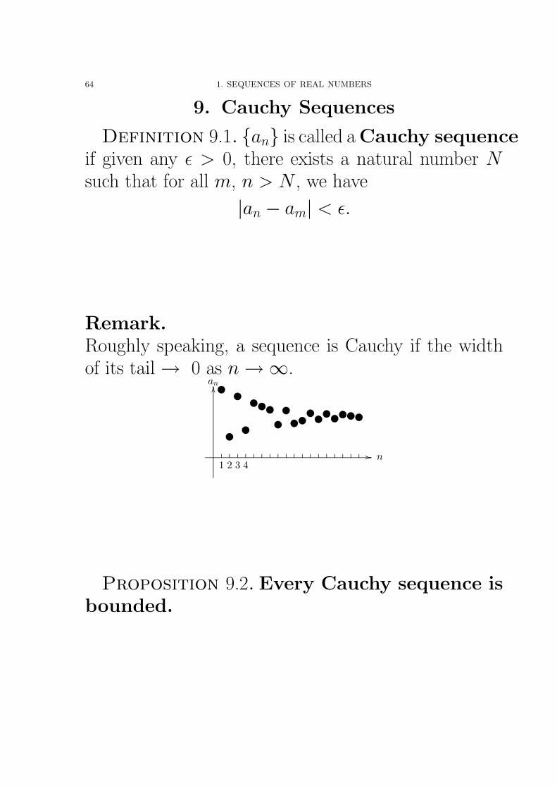
Definition 9.1. {an} is called a Cauchy sequenceif given any ε > 0, there exists a natural number Nsuch that for all m, n > N , we have
|an − am| < ε.
Remark.Roughly speaking, a sequence is Cauchy if the widthof its tail → 0 as n →∞.
............................................................................................................................................................................................................................................................................................................................................................................................................................................................................. ................
........
........
........
........
........
........
........
........
........
........
........
........
........
........
........
........
........
........
........
........
........
........
........
........
........
........
........
........
........
........
....................
................
1 2 3 4n
an
........
............
........
............
........
............
........
............
........
............
........
............
........
............
........
............
........
............
•
•
•
•••••••••••••••
Proposition 9.2. Every Cauchy sequence isbounded.
9. CAUCHY SEQUENCES 65
Proof. Let {an} be a Cauchy sequence. Chooseε = 1. There exists N such that |an − am| < 1 forn, m > N . In particular, |an − aN+1| < 1 or
aN+1 − 1 < an < aN+1 + 1
for n > N .
Let
M = max{a1, a2, · · · , aN , aN+1 + 1}m = min{a1, a2, · · · , aN , aN+1 − 1}.
For n ≤ N , we have m ≤ an ≤ M , and, for n > N ,we have
m ≤ aN+1 − 1 < an < aN+1 + 1 ≤ M.
Thus, for all n, we have m ≤ an ≤ M and so {an} isbounded. �
66 1. SEQUENCES OF REAL NUMBERS
The following Criterion was formulated by Augustin-Louis Cauchy (1789-1857).
Theorem 9.3 (Cauchy’s criterion). A sequenceis a convergent sequence if and only if it is aCauchy sequence.
Proof. =⇒, i.e., every convergent sequence is Cauchy.
Given that {an} is convergent, say limn→∞
an = A.
Then for any given ε > 0, there exists N such that
|an − A| < ε
2for all n > N. Now for any m, n > N ,
|an−am| = |(an−A)−(am−A)| ≤ |an−A|+|am−A|<
ε
2+
ε
2= ε
since both m, n > N . Therefore, {an} is a Cauchysequence.
9. CAUCHY SEQUENCES 67
⇐=, i.e., every Cauchy sequence is convergent.
Given that {an} is Cauchy. By Proposition 9.2, {an}is bounded.
By the Bolzano-Weierstrass Theorem (Corollary 8.12),there exists a convergent subsequence {ank
} of {an}.Let A = lim
k→∞ank
.
Given any ε > 0, since {an} is Cauchy, there existsN1 such that
|an − am| <ε
2for all n, m > N1.
Since {ank} converges to A, there exists K such that∣∣ank− A
∣∣ < ε
2for all k > K.
Let N = max{K, N1}. Choose an nk such thatk > N , for instance, choose nk to be nN+1. Whenn > N , by triangular inequality,
|an−A| = |(an−ank+(ank
−A)| ≤ |an−ank|+|ank
−A|<
ε
2+
ε
2= ε
because n > N ≥ N1, nk ≥ k > N ≥ N1 andk > N ≥ K.
Therefore {an} converges to A by the definition. �
68 1. SEQUENCES OF REAL NUMBERS
Example 9.4. Let sn = 1 +1
22+
1
32+ · · · +
1
n2.
Show that {sn} is convergent.
9. CAUCHY SEQUENCES 69
Proof. For each k ≥ 1, we have
|sn+k − sn|
=
∣∣∣∣(1 +1
22+ · · · + 1
n2+
1
(n + 1)2+ · · · + 1
(n + k)2
)−(
1 +1
22+ · · · + 1
n2
)∣∣∣∣=
1
(n + 1)2+
1
(n + 2)2+ · · · + 1
(n + k)2
≤ 1
n(n + 1)+
1
(n + 1)(n + 2)+
1
(n + 2)(n + 3)
+ · · · + 1
(n + k − 1)(n + k)
=
(1
n− 1
n + 1
)+
(1
n + 1− 1
n + 2
)+ · · · +
(1
n + k − 1− 1
n + k
)=
1
n− 1
n + k<
1
n.
Given any ε > 0, choose N such that 1N < ε, that is,
N >1
ε. When m > n > N , from the above,
|sm − sn| <1
n<
1
N< ε.
Thus {sn} is a Cauchy sequence and hence {sn} con-verges by the Cauchy Criterion. �

CHAPTER 2
Series of Real Numbers
1. Series
The notion of series is closely related to the sum ofnumbers. In fact, whenever one hears the word series,the first thing to come to mind is the sum of num-bers. This is the basic difference between series andsequences.
The expression
a1 + a2 + a3 + · · ·
written alternatively as
∞∑k=1
ak is called an infinite
series.
Example 1.1. (1). 1 + 2 + 3 + 4 + · · · .(2). 1 + 1/2 + 1/3 + 1/4 + · · ·(3). 1 + 1/22 + 1/32 + 1/42 + · · · .(4). 1 + 0 + 1 + 0 + 1 + 0 + · · · .
71
72 2. SERIES OF REAL NUMBERS
Definition 1.2. Given a series
∞∑k=1
ak, its nth par-
tial sum Sn is given by
Sn =
n∑k=1
ak = a1 + a2 + · · · + an.
The sequence {Sn} is called the sequence of partial
sums of the series
∞∑k=1
ak.
For instance,S1 = a1
S2 = a1 + a2
S3 = a1 + a2 + a3
S4 = a1 + a2 + a3 + a4
· · · · · ·
Example 1.3. Consider the series 1− 1 + 1− 1 +1− 1 + 1− 1 + · · · . The S2n−1 = 1 and S2n = 0.
1. SERIES 73
Definition 1.4. Consider the sequence of partial
sums {Sn} of the series
∞∑k=1
ak. If this sequence con-
verges to a number S, we say that the series
∞∑k=1
ak
converges to S and write∞∑
k=1
ak = limn→∞
Sn = S.
If {Sn} diverges, then we say
∞∑k=1
an diverges.
74 2. SERIES OF REAL NUMBERS
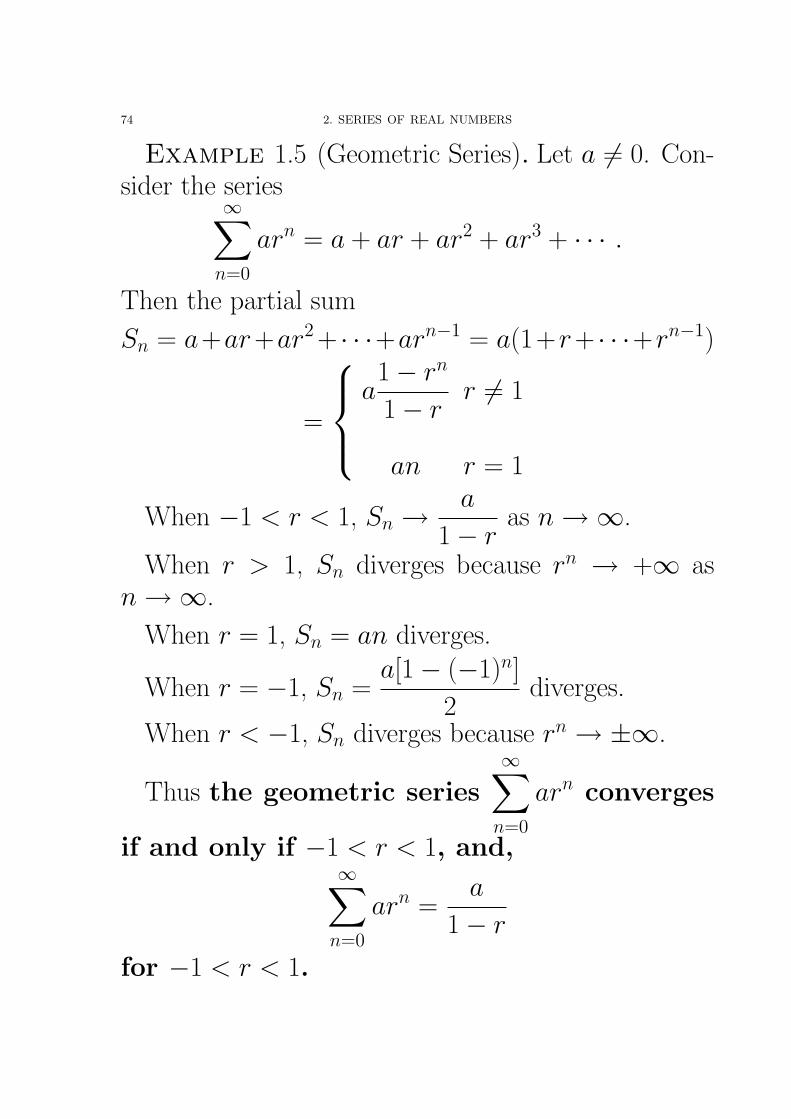
Example 1.5 (Geometric Series). Let a 6= 0. Con-sider the series
∞∑n=0
arn = a + ar + ar2 + ar3 + · · · .
Then the partial sum
Sn = a+ar+ar2 + · · ·+arn−1 = a(1+r+ · · ·+rn−1)
=
a1− rn
1− rr 6= 1
an r = 1
When −1 < r < 1, Sn →a
1− ras n →∞.
When r > 1, Sn diverges because rn → +∞ asn →∞.
When r = 1, Sn = an diverges.
When r = −1, Sn =a[1− (−1)n]
2diverges.
When r < −1, Sn diverges because rn → ±∞.
Thus the geometric series∞∑
n=0
arn converges
if and only if −1 < r < 1, and,∞∑
n=0
arn =a
1− r
for −1 < r < 1.
1. SERIES 75
Remark. If
∞∑k=1
ak and
∞∑k=1
bk converges, then one
always has
(i)
∞∑k=1
(ak + bk) =
∞∑k=1
ak +
∞∑k=1
bk.
(ii)
∞∑k=1
cak = c∞∑
k=1
ak.
Example 1.6.∞∑
n=1
[(1
4
)n
+
(1
5
)n]=
∞∑n=1
(1
4
)n
+
∞∑n=1
(1
5
)n
=
[1
4+
(1
4
)2
+ · · ·
]+
[1
5+
(1
5
)2
+ · · ·
]
=1
4
[1 +
1
4+
(1
4
)2
+ · · ·
]+
1
5
[1 +
1
5+
(1
5
)2
+ · · ·
]=
1
4
1
1− 1
4
+1
5
1
1− 1
5
=1
4 · 3
4
+1
5 · 4
5
=1
3+
1
4=
7
12.
76 2. SERIES OF REAL NUMBERS
Theorem 1.7. If∞∑
k=1
ak converges, then limk→∞
ak =
0.
Proof. Recall that partial sum Sk = a1+a2+· · ·+ak. We have
Sk − Sk−1 = (a1 + a2 + · · · + ak−1 + ak)
− (a1 + a2 + · · · + ak−1) = ak.
Since the series
∞∑k=1
ak converges, the sequence {Sk}
converges. Let S = limk→∞
Sk. Then
limk→∞
ak = limk→∞
(Sk − Sk−1)
= limk→∞
Sk − limk→∞
Sk−1 = S − S = 0.
�
Corollary 1.8 (Divergence Test). If limn→∞
an 6= 0
(or does not exist), then∞∑
n=1
an diverges. �
1. SERIES 77
Example 1.9. (1). The series
∞∑n=1
(−1)n is divergent
because the limit of the n-th term (−1)n does not exist.
(2). The series
∞∑n=1
n!
n2is divergent because
limn→∞
n!
n2=
1
limn→∞
n2
n!
=1
0= +∞ 6= 0.
(3). The series
∞∑n=1
2n + 1
3n + 2is divergent because
limn→∞
2n + 1
3n + 2= lim
n→∞
2 + 1/n
3 + 2/n=
2
36= 0.
Remark. The divergence test is a “one-way” test,
i.e., limn→∞
an = 0 does NOT imply
∞∑n=1
an converges.
78 2. SERIES OF REAL NUMBERS
Theorem 1.10 (Cauchy Criterion). The series∞∑
k=1
ak
converges if and only if given any ε > 0, there ex-ists N such that ∣∣∣∣∣
m∑k=n+1
ak
∣∣∣∣∣ < ε
for all m > n > N .
Proof. The series
∞∑k=1
ak converges if and only if
the sequence of its partial sums {Sn} converges, (bydefinition), if and only if {Sn} is Cauchy. The resultfollows from
|Sm − Sn| = |(a1 + a2 + · · · + an + an+1 + · · · + am)
−(a1 + a2 + · · · + an)|
= |an+1 + · · · + am| =
∣∣∣∣∣m∑
k=n+1
ak
∣∣∣∣∣ .�
1. SERIES 79
Example 1.11 (Harmonic Series). Show that the
series∞∑
n=1
1
ndiverges.
Proof. Note that∣∣∣∣∣2n∑
k=n+1
1
k
∣∣∣∣∣ =
∣∣∣∣ 1
n + 1+ · · · + 1
2n
∣∣∣∣=
1
n + 1+
1
n + 2+ · · · + 1
2n
≥ 1
2n+
1
2n+ · · · + 1
2n= n · 1
2n=
1
2.
Suppose that the series
∞∑n=1
1
nconverges. By the
Cauchy Criterion, given ε = 12. There exists N such
that
∣∣∣∣∣2n∑
k=n+1
1
k
∣∣∣∣∣ <1
2for all m > n > N . This contra-
dicts to the above fact that |S2n − Sn| ≥1
2, where m
is chosen to be 2n. �
80 2. SERIES OF REAL NUMBERS
Note. The divergence of the harmonic series appearsto have been established by Nicole Oresme (1323?-
1382) by showing that the sequence
{n∑
k=1
1
k
}is NOT
bounded. The name harmonic series originated fromthe Greeks. Pythagoras studied the notes emitted byplucked strings of various lengths. If a string whichemits middle C when plucked is reduced to two-thirdsof its length, it will emit the note G (musicians call theinterval from C to G a fifth). If the length of the stringis halved, it will emit top C, i.e., an octave higher.These notes are fundamental to the Pythagorean the-ory of harmony, and the corresponding lengths
1,2
3,1
2are said to be in harmonic progression. Note thattheir inverses form an arithmetic progression given by
1,3
2, 2.
The harmonic series defined above has similar proper-ties, as inverses of the terms of the associated sequence
1,1
2,1
3, · · ·
again forms the arithmetic progression 1, 2, 3, · · · .
1. SERIES 81
Theorem 1.12. Suppose that eventually ak ≥
0. Then∞∑
k=1
ak converges if and only if {Sn} is
bounded above.
Proof. We may assume that ak ≥ 0 for all k. Since
Sn+1 − Sn = an+1 ≥ 0,
the sequence {Sn} is monotone increasing.
Thus
∞∑k=1
ak converges if and only if {Sn} converges,
if and only if {Sn} is bounded above (by the MonotoneConvergence Theorem). �
Note. Suppose that eventually ak ≥ 0. This theo-rem means that the following.
1) If {Sn} is bounded above, then
∞∑k=1
ak converges.
2) If {Sn} is NOT bounded above, then
∞∑k=1
ak di-
verges.
82 2. SERIES OF REAL NUMBERS
2. Tests for Positive Series
A series
∞∑k=1
ak is called a (eventually) positive
series if every term ak is (eventually) positive.
2.1. Comparison Test.
Theorem 2.1 (Comparison Test). Consider two
series∞∑
k=1
ak and∞∑
k=1
bk. Suppose that eventually
0 ≤ ak ≤ bk.
(i) If∞∑
k=1
bk converges, then∞∑
k=1
ak converges.
(ii) If∞∑
k=1
ak diverges, then∞∑
k=1
bk diverges.
2. TESTS FOR POSITIVE SERIES 83
Proof. Assertion (ii) follows immediately from (i).
We may assume that 0 ≤ ak ≤ bk for all k. Let
An =
n∑k=1
ak, and Bn =
n∑k=1
bk. Then An ≤ Bn for all
n.
Suppose that
∞∑k=1
bk converges, that is,
∞∑k=1
bk is a
(finite) number. Then
An ≤ Bn ≤∞∑
k=1
bk
for all n and so An is bounded above.
By Theorem 1.12,
∞∑k=1
ak is convergent. �
84 2. SERIES OF REAL NUMBERS
Example 2.2. The series
∞∑k=1
(2k − 1
3k + 2
)k
converges
because (2k − 1
3k + 2
)k
≤(
2
3
)k
and the geometric series
∞∑k=1
(2
3
)k
converges.
Remark. 1. Suppose 0 ≤ an ≤ bn and
∞∑n=1
bn di-
verges. Then NO conclusion can be drawn.
2. Similarly, suppose 0 ≤ an ≤ bn and
∞∑n=1
an con-
verges. Then NO conclusion can be drawn.
Example 2.3.
0 ≤(
1
2
)n
≤ 2n ≤ 3n.
The series
∞∑n=1
3n diverges. Now
∞∑n=1
(1
2
)n
converges
and
∞∑n=1
2n diverges.
2. TESTS FOR POSITIVE SERIES 85
Corollary 2.4 (Limit Comparison Test). Sup-
pose that∞∑
k=1
ak and∞∑
k=1
bk are (eventually) positive
series.
(a). If limk→∞
ak
bk= L with 0 < L < ∞, then
∞∑k=1
ak
converges if and only if∞∑
k=1
bk converges. (So
∞∑k=1
ak diverges if and only if∞∑
k=1
bk diverges.)
(b). If limk→∞
ak
bk= 0, (that is, ak << bk), and
∞∑k=1
bk
converges, then∞∑
k=1
ak converges.
(c). If limk→∞
ak
bk= 0, (that is, ak << bk), and
∞∑k=1
ak
diverges, then∞∑
k=1
bk diverges.
Remark. If limn→∞
an
bn= +∞, interchange an and bn,
and then apply assertions (b) and (c).
86 2. SERIES OF REAL NUMBERS
Proof. We may assume that
∞∑k=1
ak and
∞∑k=1
bk are
positive series.(a). Since
limk→∞
ak
bk= L ( 6= 0, 6= ∞),{
ak
bk
}is bounded above, say, by M . Thus
0 ≤ ak ≤ Mbk
for all k. Similarly, since limk→∞
bk
ak=
1
L( 6= 0, 6= ∞),{
bk
ak
}is bounded above, say, by M ′. Thus
0 ≤ bk ≤ M ′ak
for all k.
If
∞∑k=1
ak is convergent, then
∞∑k=1
M ′ak = M ′∞∑
k=1
ak
is also convergent. By the comparison test, it follows
that
∞∑k=1
bk is also convergent because bk ≤ M ′ak.
2. TESTS FOR POSITIVE SERIES 87
If
∞∑k=1
bk is convergent, then
∞∑k=1
Mbk = M∞∑
k=1
bk
is also convergent. By the comparison test, it follows
that
∞∑k=1
ak is also convergent because ak ≤ Mbk.
88 2. SERIES OF REAL NUMBERS
Hence
∞∑k=1
ak is convergent if and only if
∞∑k=1
bk is
convergent. Hence
∞∑k=1
ak is divergent if and only if
∞∑k=1
bk is divergent.
Now we prove assertions (b) and (c).
limk→∞
ak
bk= 0
implies for every ε > 0, there is an N such that∣∣∣∣ak
bk− 0
∣∣∣∣ < ε ∀k > N.
We choose ε = 1. Then the above inequality is
ak < bk ∀k > N.
We get the result by applying the comparison test. �
2. TESTS FOR POSITIVE SERIES 89
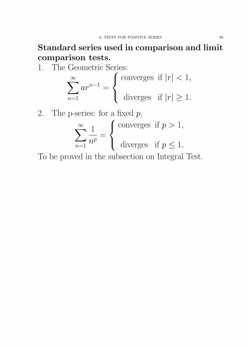
Standard series used in comparison and limitcomparison tests.1. The Geometric Series:
∞∑n=1
arn−1 =
converges if |r| < 1,
diverges if |r| ≥ 1.
2. The p-series: for a fixed p,
∞∑n=1
1
np=
converges if p > 1,
diverges if p ≤ 1.
To be proved in the subsection on Integral Test.
90 2. SERIES OF REAL NUMBERS
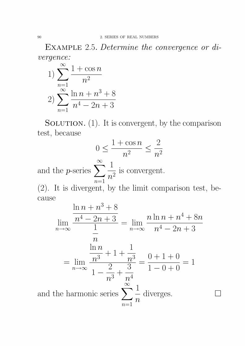
Example 2.5. Determine the convergence or di-vergence:
1)
∞∑n=1
1 + cos n
n2
2)
∞∑n=1
ln n + n3 + 8
n4 − 2n + 3
Solution. (1). It is convergent, by the comparisontest, because
0 ≤ 1 + cos n
n2≤ 2
n2
and the p-series
∞∑n=1
1
n2is convergent.
(2). It is divergent, by the limit comparison test, be-cause
limn→∞
ln n + n3 + 8
n4 − 2n + 31
n
= limn→∞
n ln n + n4 + 8n
n4 − 2n + 3
= limn→∞
ln n
n3+ 1 +
1
n3
1− 2
n3+
3
n4
=0 + 1 + 0
1− 0 + 0= 1
and the harmonic series
∞∑n=1
1
ndiverges. �
2. TESTS FOR POSITIVE SERIES 91
Example 2.6. Determine convergence or diver-
gence of∞∑
n=2
1
(ln n)k, where k is a constant.
Solution. Let bn =1
(ln n)kand let an =
1
n. Then
limn→∞
an
bn= lim
n→∞
1
n1
(ln n)k
= limn→∞
(ln n)k
n= 0.
Since the harmonic series
∞∑n=2
1
nis divergent, the series
∞∑n=2
1
(ln n)kis divergent for any k. �
92 2. SERIES OF REAL NUMBERS
2.2. Integral Test. Let f (x) be a real-valued func-tion on [a, +∞) such that f (x) is Riemann integrable,
that is, the integral
∫ b
a
f (x) dx exists for every b > a.
The following theorem is useful.
Theorem 2.7. Let f (x) be a real-valued functionon [a, b].
(a). If f (x) is continuous on [a, b], then f (x)is Riemann integrable on [a, b].
(b). If f (x) is monotone on [a, b], then f (x) isRiemann integrable on [a, b].
2. TESTS FOR POSITIVE SERIES 93
The improper integral is defined by∫ ∞
a
f (x) dx = limb→∞
∫ b
a
f (x) dx
= area under f (x) over [a,∞).
Here we say that
∫ ∞
a
f (x) dx converges if the limit
limb→∞
∫ b
a
f (x) dx
exists (finite), i.e., the area under f (x) over [a,∞) isfinite.
We also say that
∫ ∞
a
f (x) dx diverges if the limit
limb→∞
∫ b
a
f (x) dx
does not exist.
94 2. SERIES OF REAL NUMBERS
Theorem 2.8 (Integral Test). Let f (x) be an (even-tually) positive monotone decreasing function
on [1, +∞). Suppose we have a series∞∑
k=1
ak such
that ak = f (k), then the series∞∑
k=1
ak and the
integral
∫ ∞
1
f (x)dx either both converge or
both diverge.
2. TESTS FOR POSITIVE SERIES 95
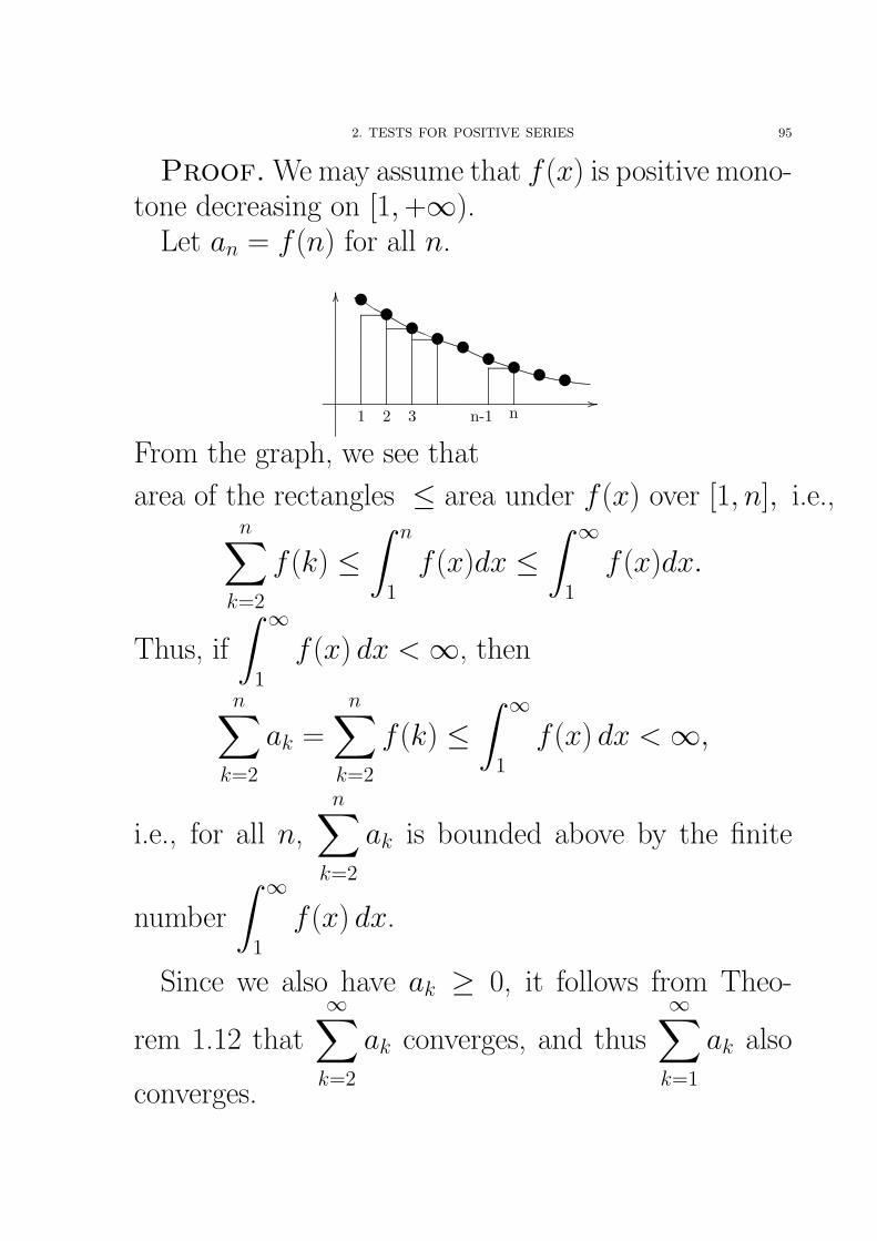
Proof. We may assume that f (x) is positive mono-tone decreasing on [1, +∞).
Let an = f (n) for all n.
................................................................................................................................................................................................................................................................................................................................................................................................................................................................................................... ................
........
........
........
........
........
........
........
........
........
........
........
........
........
........
........
........
........
........
........
........
........
........
........
........
........
........
........
........
........
........
....................
................
1 2 3 n-1 n
...................................................................................................................................................................................................................................................................................................................................................................................................................................................
........
........
........
........
........
........
........
........
........
........
........
........
........
........
........
........
........
........
............................................................................................................................................................................................................
.............................................................................................................................................................................
........................................................................................................................................................... ........................................................................................................................................................................
• • • • • • • • •
From the graph, we see that
area of the rectangles ≤ area under f (x) over [1, n], i.e.,n∑
k=2
f (k) ≤∫ n
1
f (x)dx ≤∫ ∞
1
f (x)dx.
Thus, if
∫ ∞
1
f (x) dx < ∞, then
n∑k=2
ak =
n∑k=2
f (k) ≤∫ ∞
1
f (x) dx < ∞,
i.e., for all n,
n∑k=2
ak is bounded above by the finite
number
∫ ∞
1
f (x) dx.
Since we also have ak ≥ 0, it follows from Theo-
rem 1.12 that
∞∑k=2
ak converges, and thus
∞∑k=1
ak also
converges.
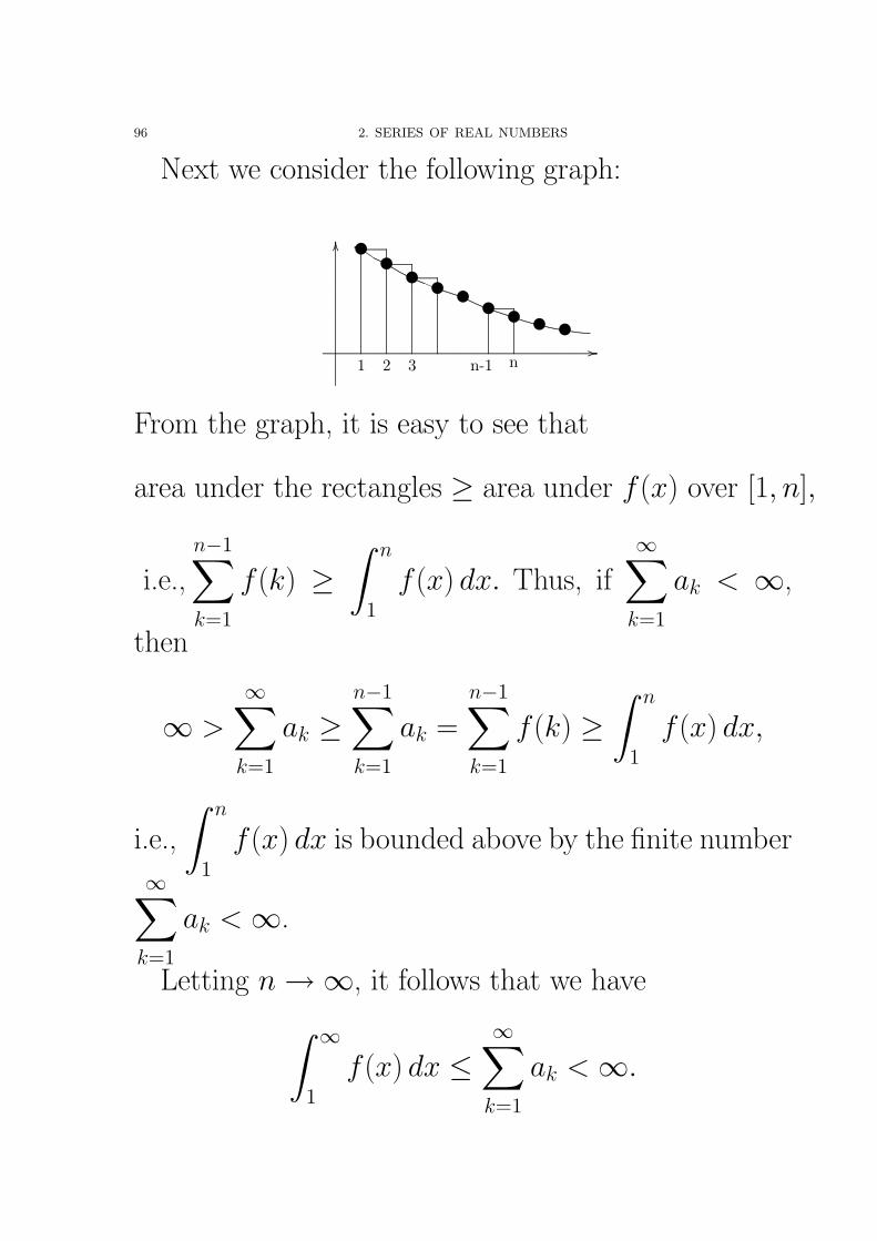
96 2. SERIES OF REAL NUMBERS
Next we consider the following graph:
................................................................................................................................................................................................................................................................................................................................................................................................................................................................................................... ................
........
........
........
........
........
........
........
........
........
........
........
........
........
........
........
........
........
........
........
........
........
........
........
........
........
........
........
........
........
........
....................
................
1 2 3 n-1 n
...................................................................................................................................................................................................................................................................................................................................................................................................................................................
........
........
........
........
........
........
........
........
........
........
........
........
........
........
........
........
........
........
........
........
........
........
................................................................................................................................................................................................................................
....................................................................................................................................................................................................
............................................................................................................................................................................. ....................................................................................................................................................................................................
• • • • • • • • •
From the graph, it is easy to see that
area under the rectangles ≥ area under f (x) over [1, n],
i.e.,
n−1∑k=1
f (k) ≥∫ n
1
f (x) dx. Thus, if
∞∑k=1
ak < ∞,
then
∞ >∞∑
k=1
ak ≥n−1∑k=1
ak =
n−1∑k=1
f (k) ≥∫ n
1
f (x) dx,
i.e.,
∫ n
1
f (x) dx is bounded above by the finite number
∞∑k=1
ak < ∞.
Letting n →∞, it follows that we have∫ ∞
1
f (x) dx ≤∞∑
k=1
ak < ∞.
2. TESTS FOR POSITIVE SERIES 97
In conclusion, we have
∞∑k=1
ak converges if and only if∫ ∞
1
f (x) dx converges, which also means that
∞∑k=1
ak di-
verges if and only if
∫ ∞
1
f (x) dx diverges. �
98 2. SERIES OF REAL NUMBERS
Example 2.9. Show that
1) the series∞∑
n=1
1
npconverges if and only if p >
1.
2) the series∞∑
n=2
1
n(ln n)kconverges if and only if
k > 1.
Proof. (1). If p ≤ 0, then1
npdoes not tend to 0
and so, by divergence test,
∞∑n=1
1
npdiverges.
Assume that p > 0. Let f (x) =1
xpon [1, +∞).
Then f (x) is positive monotone decreasing. Now∫ ∞
1
f (x)dx =
∫ ∞
1
x−p dx =
1
−p + 1x−p+1
∣∣∣∣+∞1
p 6= 1
ln(+∞)− ln 1 p = 1
Thus
∫ ∞
1
f (x) dx converges if and only if p > 1 and
so
∞∑n=1
1
npconverges if and only if p > 1.
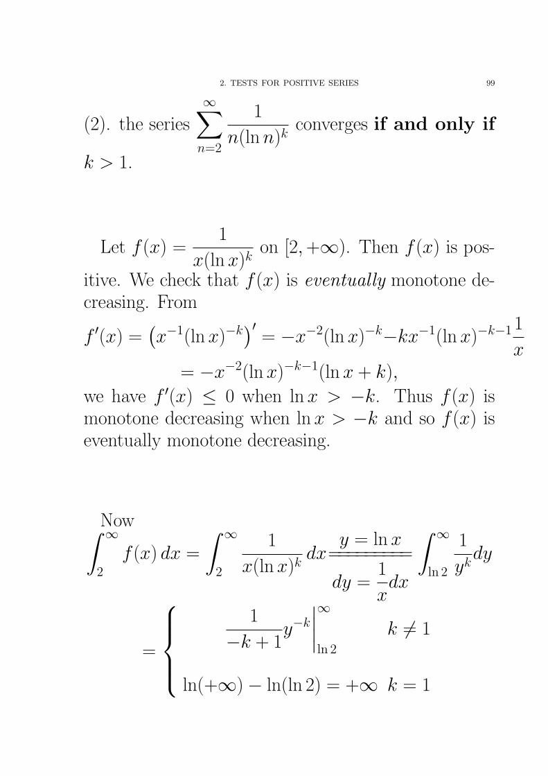
2. TESTS FOR POSITIVE SERIES 99
(2). the series
∞∑n=2
1
n(ln n)kconverges if and only if
k > 1.
Let f (x) =1
x(ln x)kon [2, +∞). Then f (x) is pos-
itive. We check that f (x) is eventually monotone de-creasing. From
f ′(x) =(x−1(ln x)−k
)′= −x−2(ln x)−k−kx−1(ln x)−k−11
x= −x−2(ln x)−k−1(ln x + k),
we have f ′(x) ≤ 0 when ln x > −k. Thus f (x) ismonotone decreasing when ln x > −k and so f (x) iseventually monotone decreasing.
Now∫ ∞
2
f (x) dx =
∫ ∞
2
1
x(ln x)kdx=========
y = ln x
dy =1
xdx
∫ ∞
ln 2
1
ykdy
=
1
−k + 1y−k
∣∣∣∣∞ln 2
k 6= 1
ln(+∞)− ln(ln 2) = +∞ k = 1
100 2. SERIES OF REAL NUMBERS
Thus
∫ ∞
2
f (x) dx converges if and only if k > 1 and
so the series
∞∑n=2
1
n(ln n)kconverges if and only if k >
1. �
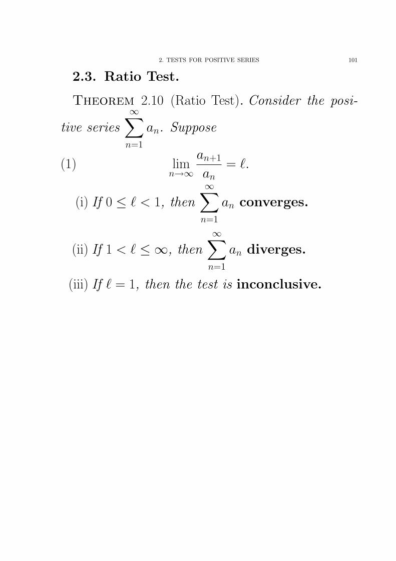
2. TESTS FOR POSITIVE SERIES 101
2.3. Ratio Test.
Theorem 2.10 (Ratio Test). Consider the posi-
tive series∞∑
n=1
an. Suppose
(1) limn→∞
an+1
an= `.
(i) If 0 ≤ ` < 1, then∞∑
n=1
an converges.
(ii) If 1 < ` ≤ ∞, then∞∑
n=1
an diverges.
(iii) If ` = 1, then the test is inconclusive.
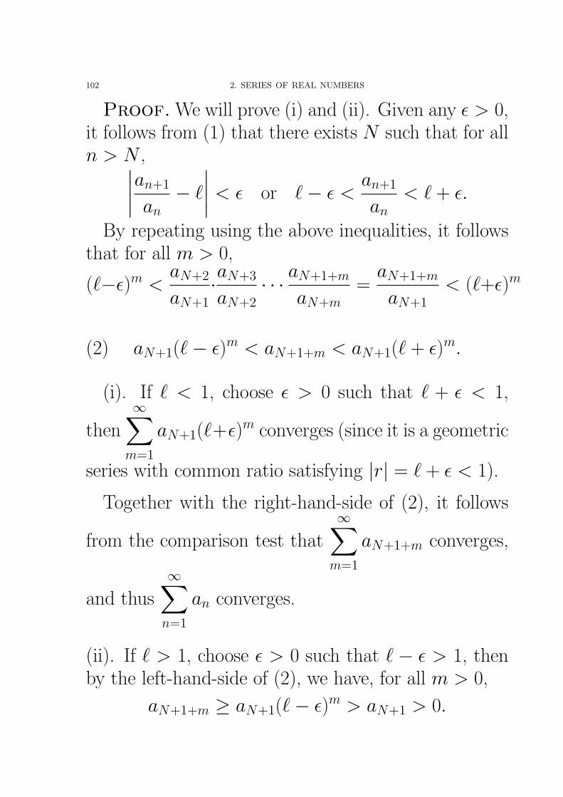
102 2. SERIES OF REAL NUMBERS
Proof. We will prove (i) and (ii). Given any ε > 0,it follows from (1) that there exists N such that for alln > N ,∣∣∣∣an+1
an− `
∣∣∣∣ < ε or `− ε <an+1
an< ` + ε.
By repeating using the above inequalities, it followsthat for all m > 0,
(`−ε)m <aN+2
aN+1·aN+3
aN+2· · · aN+1+m
aN+m=
aN+1+m
aN+1< (`+ε)m
(2) aN+1(`− ε)m < aN+1+m < aN+1(` + ε)m.
(i). If ` < 1, choose ε > 0 such that ` + ε < 1,
then
∞∑m=1
aN+1(`+ε)m converges (since it is a geometric
series with common ratio satisfying |r| = ` + ε < 1).
Together with the right-hand-side of (2), it follows
from the comparison test that
∞∑m=1
aN+1+m converges,
and thus
∞∑n=1
an converges.
(ii). If ` > 1, choose ε > 0 such that ` − ε > 1, thenby the left-hand-side of (2), we have, for all m > 0,
aN+1+m ≥ aN+1(`− ε)m > aN+1 > 0.
2. TESTS FOR POSITIVE SERIES 103
In particular, limn→∞
an 6= 0 or does not exist. By the
divergence test,
∞∑n=1
an diverges. �
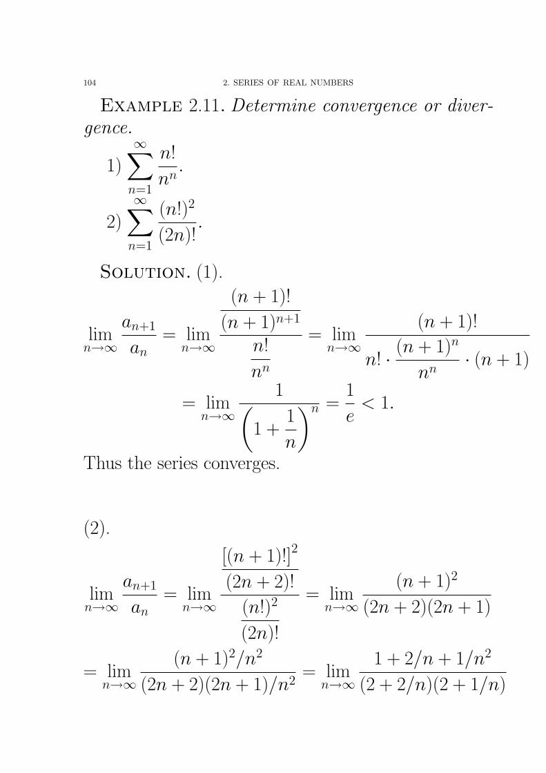
104 2. SERIES OF REAL NUMBERS
Example 2.11. Determine convergence or diver-gence.
1)
∞∑n=1
n!
nn.
2)
∞∑n=1
(n!)2
(2n)!.
Solution. (1).
limn→∞
an+1
an= lim
n→∞
(n + 1)!
(n + 1)n+1
n!
nn
= limn→∞
(n + 1)!
n! · (n + 1)n
nn· (n + 1)
= limn→∞
1(1 +
1
n
)n =1
e< 1.
Thus the series converges.
(2).
limn→∞
an+1
an= lim
n→∞
[(n + 1)!]2
(2n + 2)!
(n!)2
(2n)!
= limn→∞
(n + 1)2
(2n + 2)(2n + 1)
= limn→∞
(n + 1)2/n2
(2n + 2)(2n + 1)/n2= lim
n→∞
1 + 2/n + 1/n2
(2 + 2/n)(2 + 1/n)
2. TESTS FOR POSITIVE SERIES 105
=1 + 0 + 0
(2 + 0) · (2 + 0)=
1
4< 1.
Thus the series converges.�
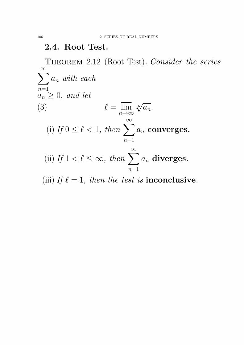
106 2. SERIES OF REAL NUMBERS
2.4. Root Test.
Theorem 2.12 (Root Test). Consider the series∞∑
n=1
an with each
an ≥ 0, and let
(3) ` = limn→∞
n√
an.
(i) If 0 ≤ ` < 1, then∞∑
n=1
an converges.
(ii) If 1 < ` ≤ ∞, then∞∑
n=1
an diverges.
(iii) If ` = 1, then the test is inconclusive.
2. TESTS FOR POSITIVE SERIES 107
Proof. We will prove (i) and (ii).(i). Suppose that ` < 1. Then for all given ε > 0,
it follows from (3) and Proposition 8.9 of chapter 1,that there exists an N such that n
√an < ` + ε for all
n > N . Now choose ε > 0 s.t. ` + ε < 1. Then
(4) 0 ≤ an < (` + ε)n for all n > N.
Since
∞∑n=1
(` + ε)n converges (as it is a geometric series
with common ratio satisfying |r| = ` + ε < 1), it
follows from (4) and the comparison test that
∞∑n=1
an
converges.
(ii). We are going to prove (ii) by contradiction. Given
that ` > 1. Suppose that
∞∑n=1
an converges. Then by
Theorem 1.7, we have limn→∞
an = 0. In particular, there
exists N such that 0 ≤ an < 1 for all n > N . Hencen√
an < 1 for all n > N , and it follows that we must
have ` ≤ 1, which is a contradiction. Hence
∞∑n=1
an
diverges. �
108 2. SERIES OF REAL NUMBERS
Corollary 2.13 (Simplified Root Test). Consider
the series∞∑
n=1
an with each an ≥ 0. Suppose that
limn→∞
n√
an = `.
(i) If 0 ≤ ` < 1, then∞∑
n=1
an converges.
(ii) If 1 < ` ≤ ∞, then∞∑
n=1
an diverges.
(iii) If ` = 1, then the test is inconclusive.
Proof. We will prove (i) and (ii). Recall from The-orem 8.13 of chapter 1 that if lim
n→∞n√
an exists, then
limn→∞
n√
an = limn→∞
n√
an. Then the Corollary follows
from Theorem 2.12. �
2. TESTS FOR POSITIVE SERIES 109
Example 2.14. Determine convergence or diver-gence of the series
∞∑n=1
2n
(1− 1
n
)n2
.
Solution.
limn→∞
n√
an = limn→∞
[2n
(1− 1
n
)n2]1
n
= limn→∞
2
(1− 1
n
)n
=2
e< 1.
Thus the series converges.�
Example 2.15. Determine convergence or diver-gence of the series
∞∑n=1
(3 + sin n)n(
1− 2
n
)n2
.
110 2. SERIES OF REAL NUMBERS
Proof.
limn→∞
n√
an = limn→∞
[(3 + sin n)n
(1− 2
n
)n2]1
n
= limn→∞
(3+sin n)
(1− 2
n
)n
≤ limn→∞
4
(1− 2
n
)n
=4
e2< 1.
Thus the series converges. �
3. ALTERNATING SERIES 111
3. Alternating Series
An alternating series is of the form∞∑
n=1
(−1)n+1an = a1 − a2 + a3 − a4 + · · · , or
∞∑n=1
(−1)nan = −a1 + a2 − a3 + a4 − · · ·
with each an > 0.
Example 3.1.
1− 1 + 1− 1 + 1− 1 + 1− 1 + · · ·1− 1
2+
1
3− 1
4+ · · ·
−1 + 2− 3 + 4− 5 + 6− · · ·
Theorem 3.2 (The Alternating Series test). If {bn}is a sequence satisfying
(i) b1 ≥ b2 ≥ b3 ≥ · · · ≥ 0, and(ii) lim
n→∞bn = 0,
then∞∑
n=1
(−1)n+1bn ( and∞∑
n=1
(−1)nbn) converge.
Note. The test holds if {bn} is eventually posi-tive and eventually monotone decreasing withlim
n→∞bn = 0.
112 2. SERIES OF REAL NUMBERS
Proof. We prove that the sequence of partial sums
Sn =n∑
k=1
(−1)k+1bk is Cauchy.
For m > n, note that
|Sm − Sn|=∣∣(−1)n+2bn+1 + (−1)n+3bn+2 + · + (−1)m+1bm
∣∣=∣∣bn+1 − bn+2 + bn+3 − bn+4 + · · · + (−1)m−n−1bm
∣∣≤ bn+1 + bm
because
bn+1 − bn+2 + bn+3 − bn+4 + · · · + (−1)m−n−1bm
= (bn+1 − bn+2) + (bn+3 − bn+4) + · · · ± bm ≥ −bm
and
bn+1 − bn+2 + bn+3 − bn+4 + · · · + (−1)m−n−1bm
= bn+1−(bn+2)−(bn+3)−(bn+4−bn+5)+· · · ≤ bn+1+bm,
where we use the property that {bn} is positive andmonotone decreasing.
Given any ε > 0, there exists N such that bn =|bn − 0| < ε
2. Then for m > n > N ,
|Sm − Sn| ≤ bn+1 + bm <ε
2+
ε
2= ε.
Thus {Sn} is Cauchy and hence the result.�
3. ALTERNATING SERIES 113
Example 3.3. Show that convergence or diver-gence of the series
∞∑n=1
(−1)n1
np=
convergence p > 0
divergence p ≤ 0.
Proof. If p ≤ 0, then the n-th term (−1)n1
npdoes
not tend to 0. Thus the series diverges in this case bythe divergence test.
Assume that p > 0. Let an =1
np. Then an >
0, monotone decreasing and limn→∞
an = 0. Thus the
alternating series converges in this case.
In conclusion, we have that the series
∞∑n=1
(−1)n1
np
converges when p > 0 and diverges when p ≤ 0. �
114 2. SERIES OF REAL NUMBERS
Now we are going to give a theorem providing anestimate on the sum of (certain) series. For instance,
let S =
∞∑n=1
(−1)n+1 1
n2. By taking the partial sum, we
have
S ≈ S1 = 1, S ≈ S2 = 1− 1
22= 0.75,
S ≈ S3 = 1− 1
22+
1
32≈ 0.861, . . . .
By using computer program, we are able to computemuch more, say S1000000. A mathematical problem isthen what is the ‘error’ for estimating S by using thepartial sum Sn. In other words, how to estimate theremainder
Rn = |S − Sn| = |an+1 + an+2 + · · · |.
Theorem 3.4 (Alternating Series Estimation). Let{bn} be a sequence satisfying
(i) b1 ≥ b2 ≥ b3 ≥ · · · ≥ 0, and
(ii) limn→∞
bn = 0.
Let
Sn =
n∑k=1
(−1)k+1bk and S =
∞∑k=1
(−1)k+1bk
Then the remainder Rn = |S − Sn| ≤ bn+1 for alln.
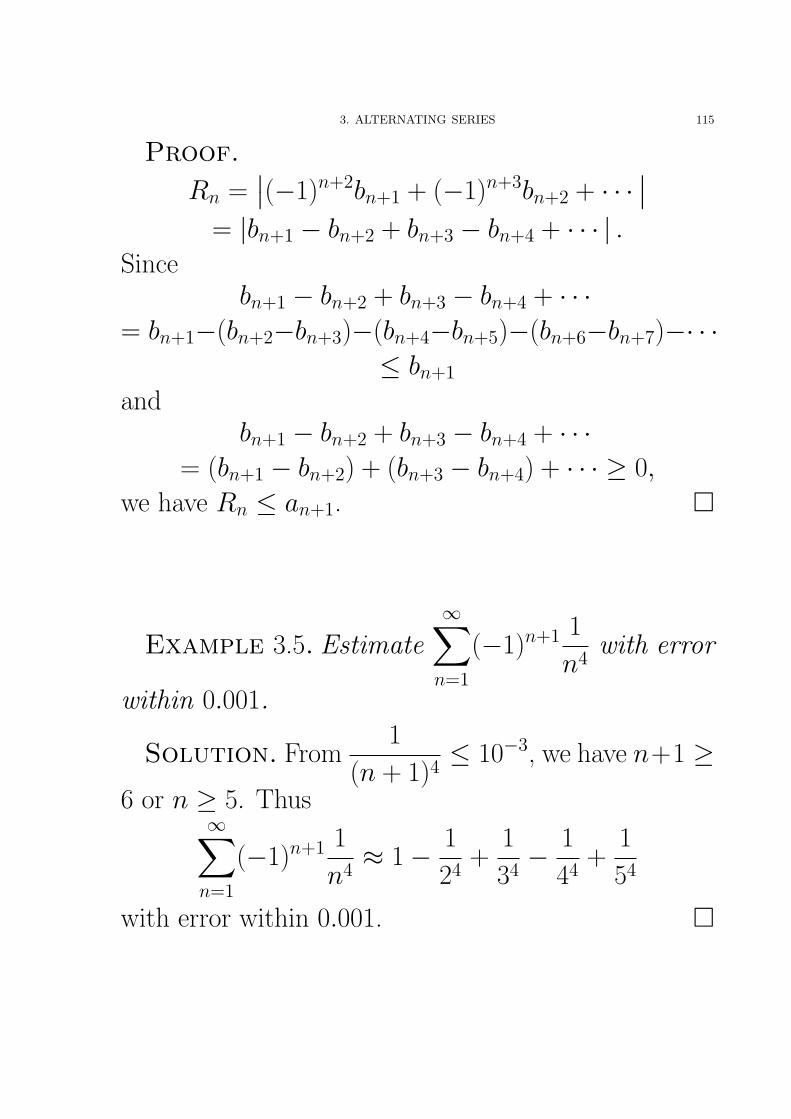
3. ALTERNATING SERIES 115
Proof.
Rn =∣∣(−1)n+2bn+1 + (−1)n+3bn+2 + · · ·
∣∣= |bn+1 − bn+2 + bn+3 − bn+4 + · · · | .
Sincebn+1 − bn+2 + bn+3 − bn+4 + · · ·
= bn+1−(bn+2−bn+3)−(bn+4−bn+5)−(bn+6−bn+7)−· · ·≤ bn+1
andbn+1 − bn+2 + bn+3 − bn+4 + · · ·
= (bn+1 − bn+2) + (bn+3 − bn+4) + · · · ≥ 0,
we have Rn ≤ an+1. �
Example 3.5. Estimate∞∑
n=1
(−1)n+1 1
n4with error
within 0.001.
Solution. From1
(n + 1)4≤ 10−3, we have n+1 ≥
6 or n ≥ 5. Thus∞∑
n=1
(−1)n+1 1
n4≈ 1− 1
24+
1
34− 1
44+
1
54
with error within 0.001. �
116 2. SERIES OF REAL NUMBERS
4. Absolute and Conditional Convergence
Definition 4.1. A series∞∑
n=1
an is called abso-
lutely convergent if∞∑
n=1
|an| converges.
Theorem 4.2. Every absolutely convergentseries is convergent.
4. ABSOLUTE AND CONDITIONAL CONVERGENCE 117
Proof. Suppose that
∞∑n=1
an converges absolutely,
that is,
∞∑n=1
|an| converges by the definition. Let Tn =
n∑k=1
|ak|, Sn =
n∑k=1
ak.
Since {Tn} converges, {Tn} is Cauchy.
Thus, for any ε > 0, there is a N such that |Tn −Tm| < ε for all n, m > N . For any n, m > N , we mayassume that m ≥ n, say m = n + p (as one of themshould be greater than another). Then
|Sn − Sm| = |Sn − (Sn + an+1 + an+2 + · · · + an+p)|= |an+1 + an+2 + · · · + an+p|
≤ |an+1|+|an+2|+· · ·+|an+p| = Tm−Tn = |Tn−Tm| < ε.
Thus {Sn} is a Cauchy sequence and so it converges.
Thus the series
∞∑n=1
an converges and hence the result.
�
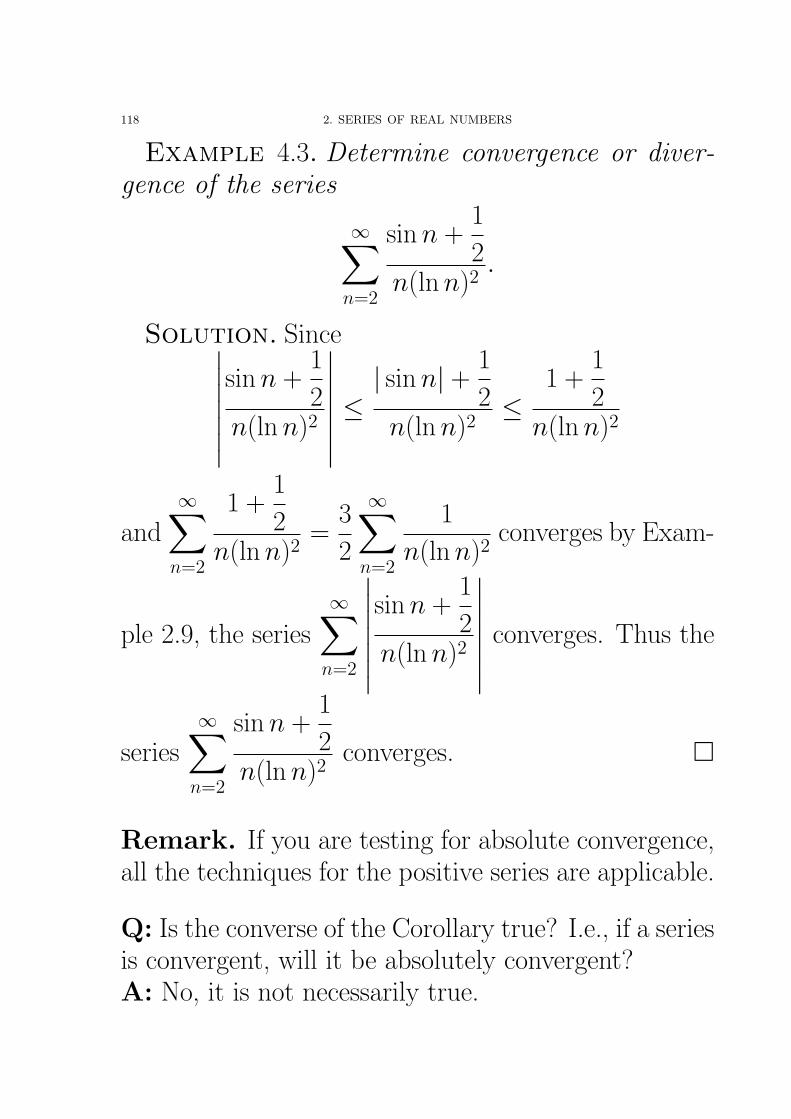
118 2. SERIES OF REAL NUMBERS
Example 4.3. Determine convergence or diver-gence of the series
∞∑n=2
sin n +1
2n(ln n)2
.
Solution. Since∣∣∣∣∣∣∣sin n +
1
2n(ln n)2
∣∣∣∣∣∣∣ ≤| sin n| + 1
2n(ln n)2
≤1 +
1
2n(ln n)2
and
∞∑n=2
1 +1
2n(ln n)2
=3
2
∞∑n=2
1
n(ln n)2converges by Exam-
ple 2.9, the series
∞∑n=2
∣∣∣∣∣∣∣sin n +
1
2n(ln n)2
∣∣∣∣∣∣∣ converges. Thus the
series
∞∑n=2
sin n +1
2n(ln n)2
converges. �
Remark. If you are testing for absolute convergence,all the techniques for the positive series are applicable.
Q: Is the converse of the Corollary true? I.e., if a seriesis convergent, will it be absolutely convergent?A: No, it is not necessarily true.
4. ABSOLUTE AND CONDITIONAL CONVERGENCE 119
Example 4.4. The series
∞∑n=1
(−1)n1
nconverges by
Example 3.3, but it is NOT absolutely convergent bythe p-series.
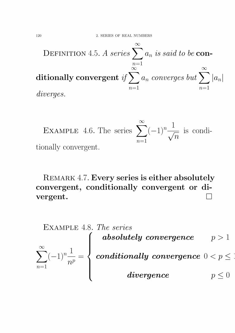
120 2. SERIES OF REAL NUMBERS
Definition 4.5. A series∞∑
n=1
an is said to be con-
ditionally convergent if∞∑
n=1
an converges but∞∑
n=1
|an|
diverges.
Example 4.6. The series
∞∑n=1
(−1)n1√n
is condi-
tionally convergent.
Remark 4.7. Every series is either absolutelyconvergent, conditionally convergent or di-vergent. �
Example 4.8. The series
∞∑n=1
(−1)n1
np=
absolutely convergence p > 1
conditionally convergence 0 < p ≤ 1
divergence p ≤ 0
5. REARRANGEMENT PROPERTIES OF A SERIES - AN INFORMAL TREATMENT 121
5. Rearrangement properties of a series -an informal treatment
Roughly speaking, a rearrangement of a given se-ries is another series produced from a given series byscrambling the order of the terms of the given series,but using all the terms exactly once. Example: Con-
sider the harmonic series
1 +1
2+
1
3+
1
4+
1
5+
1
6+
1
7+
1
8+ · · · .
An rearrangement of the harmonic series is obtainedby interchanging the 1st and 2nd terms, the 3rd and4th terms, and so on, resulting in the new series
1
2+ 1 +
1
4+
1
3+
1
6+
1
5+
1
8+
1
7+ · · · .
It turns out that the sum of a rearrangement of a givenseries may be different from the original series. Infact, for any given conditional convergent series∞∑
n=1
an and any given real number c ∈ R, it is known
that one may rearrange
∞∑n=1
an so that the new series
∞∑n=1
bn will converge to c (i.e.,
∞∑n=1
bn = c). On the
other hand, an absolutely convergent series has
122 2. SERIES OF REAL NUMBERS
much nicer rearrangement properties. Given an abso-
lutely convergent series
∞∑n=1
an, whose sum is denoted
by S, i.e.,
∞∑n=1
an = S. Then for any rearrangement
∞∑n=1
bn of
∞∑n=1
an, one always has
∞∑n=1
bn = S. In other
words, rearranging an absolutely convergent series willnot change the sum.Reading Exercise: See Bartle-Sherbert[1, p.255]for details.
6. Remarks on the various tests forconvergence/divergence of series
1. n-th term test for divergence:- a test for divergence ONLY, and it works for series
with positive and negative terms, e.g.
∞∑n=1
(−1)n.
2. Comparison test/Limit Comparison test:- when applying these tests, one usually compares
the given series with a geometric series or a p-series.- generally works for series which look like the geomet-ric series or the p-series,
e.g.
∞∑n=1
2 + (−1)n
4n,
∞∑n=1
21n
n2.
6. REMARKS ON THE VARIOUS TESTS FOR CONVERGENCE/DIVERGENCE OF SERIES 123
- when an oscillating factor/term appears, e.g.
∞∑n=1
2 + (−1)n
3n,
try the Comparison test rather than the Limit Com-parison test.
3. Integral test:
e.g.
∞∑n=2
1
n(ln n)2.
124 2. SERIES OF REAL NUMBERS
4. Ratio test:- generally works for series which look like the geo-metric series, series with n!, and certain series definedrecursively,
e.g.
∞∑n=1
n2
3n,
∞∑n=1
(2n)!
4n · n!,
∞∑n=1
an, where a1 = 1, an = (1
2+
1
n)an−1, n = 2, 3, · · · .
5. (Simplified) Root test:- generally works for series where an involves a highpower such as the n-th power,
e.g.
∞∑n=1
n
3n,
∞∑n=1
2n(1− 1
n
)n2
.
6. Alternating Series test: - works for alternat-ing series only,
e.g.
∞∑n=2
(−1)nln n
n.
Remark. In general, Tests 2 - 5 works only for
∞∑n=1
an,
where an ≥ 0 (except Ratio and Root Tests for generalseries).
CHAPTER 3
Sequences and Series of Functions
1. Pointwise Convergence
1.1. Sequences of Functions. Let I be a (nonempty)subset of R, e.g. (−1, 1), [0, 1], etc. For each n ∈ N,let Fn : I → R be a function. Then we say {Fn} formsa sequence of functions on I .
125
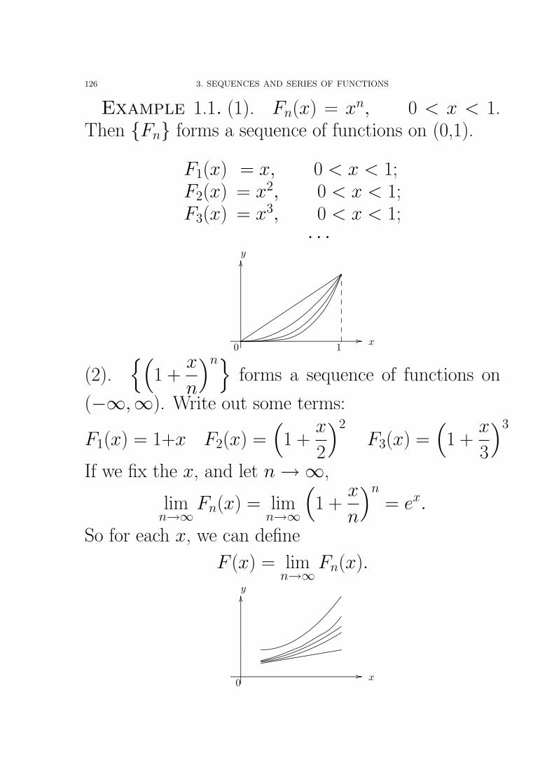
126 3. SEQUENCES AND SERIES OF FUNCTIONS
Example 1.1. (1). Fn(x) = xn, 0 < x < 1.Then {Fn} forms a sequence of functions on (0,1).
F1(x) = x, 0 < x < 1;F2(x) = x2, 0 < x < 1;F3(x) = x3, 0 < x < 1;
· · ·
................................................................................................................................................................................................................................................................................................................................................................................. ................
........
........
........
........
........
........
........
........
........
........
........
........
........
........
........
........
........
........
........
........
........
........
........
........
........
........
........
........
........
...................
................
0 1 x
y
......................................................................................................................................................................................................................................................................................................................................
.................................................................................
.....................................
............................................................................................................................................................................................................................
.........................................................................................................................
...................................
...................................................................................................................................................................................................
......................................................................................................................................................
....................................................................................................................................................................................................................
........
.....
........
.....
........
.....
........
.....
........
.....
........
.....
........
.....
......
(2).{(
1 +x
n
)n}forms a sequence of functions on
(−∞,∞). Write out some terms:
F1(x) = 1+x F2(x) =(1 +
x
2
)2
F3(x) =(1 +
x
3
)3
If we fix the x, and let n →∞,
limn→∞
Fn(x) = limn→∞
(1 +
x
n
)n
= ex.
So for each x, we can define
F (x) = limn→∞
Fn(x).
................................................................................................................................................................................................................................................................................................................................................................................. ................
........
........
........
........
........
........
........
........
........
........
........
........
........
........
........
........
........
........
........
........
........
........
........
........
........
........
........
........
........
...................
................
0 x
y
..............................................................................................
..............................................................................................
.........................................................................................................
..................................
...................................................................................................................................................................
................................................................................
...............................................
......................................
.................................
...............................
.....
.................................................................
.............................................
.....................................
.................................
..............................
.............................
.......................................................
..........................................
...................................
..............................
...............................
...........................................................
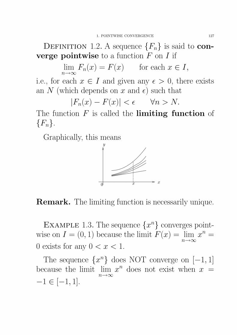
1. POINTWISE CONVERGENCE 127
Definition 1.2. A sequence {Fn} is said to con-verge pointwise to a function F on I if
limn→∞
Fn(x) = F (x) for each x ∈ I,
i.e., for each x ∈ I and given any ε > 0, there existsan N (which depends on x and ε) such that
|Fn(x)− F (x)| < ε ∀n > N.
The function F is called the limiting function of{Fn}.
Graphically, this means
................................................................................................................................................................................................................................................................................................................................................................................. ................
........
........
........
........
........
........
........
........
........
........
........
........
........
........
........
........
........
........
........
........
........
........
........
........
........
........
........
........
........
...................
................
0 xx
y
..............................................................................................
..............................................................................................
.........................................................................................................
..................................
...................................................................................................................................................................
................................................................................
...............................................
......................................
.................................
...............................
.....
.................................................................
.............................................
.....................................
.................................
..............................
.............................
.......................................................
..........................................
...................................
..............................
...............................
...........................................................
......
......
......
......
......
......
......
......
......
......
......
......
......
Remark. The limiting function is necessarily unique.
Example 1.3. The sequence {xn} converges point-wise on I = (0, 1) because the limit F (x) = lim
n→∞xn =
0 exists for any 0 < x < 1.
The sequence {xn} does NOT converge on [−1, 1]because the limit lim
n→∞xn does not exist when x =
−1 ∈ [−1, 1].
128 3. SEQUENCES AND SERIES OF FUNCTIONS
1.2. Series of Functions. A series of func-tions on a set I is of the form
∞∑n=1
fn(x) = f1(x) + f2(x) + · · · ,
where each fn is a function on I .
Example 1.4. Below are some examples.
1.
∞∑n=1
xn−1 = 1 + x + x2 + x3 + · · ·
2.
∞∑k=1
sin kx
k + x=
sin x
1 + x+
sin 2x
2 + x+
sin 3x
3 + x+· · · , 0 ≤
x ≤ 1.
As in chapter 2, we may form the partial sums
Sn(x) =
n∑k=1
fk(x) = f1(x) + f2(x) + · · · + fn(x).
Then {Sn} forms a sequence of functions on I .
Definition 1.5. The series
∞∑n=1
fn is said to con-
verge pointwise (to a function S) on I if {Sn} con-verges pointwise (to S) on I , (i.e. lim
n→∞Sn(x) = S(x)
for each x ∈ I .)
1. POINTWISE CONVERGENCE 129
Example 1.6. What is the pointwise limit of∞∑
n=1
xn−1,
where x ∈ (−1, 1)? Does∞∑
n=1
xn−1 converge point-
wise on [−1, 1)
Solution. Consider the partial sum
Sn(x) =
n∑i=1
xi−1 = 1 + x + · · · + xn−1 =1− xn
1− x
for −1 < x < 1. Thus∞∑
n=1
xn−1 = limn→∞
Sn(x) = limn→∞
1− xn
1− x=
1
1− x
for x ∈ (−1, 1).
Since the series
∞∑n=1
xn−1 diverges when x = −1,
the series of functions
∞∑n=1
xn−1 does NOT converge
pointwise on [−1, 1). �
130 3. SEQUENCES AND SERIES OF FUNCTIONS
1.3. Some Questions on Pointwise Conver-gence. Suppose a sequence of functions {Fn} con-verges pointwise to a function F on the interval [a, b].
Also suppose a series of functions
∞∑n=1
fn(x) converges
pointwise to a function S(x) on [a, b]. Among thequestions we want to consider the following. Some ofthese questions were incorrectly believed to be true bymany mathematicians prior to nineteenth century, in-cluding the famous Cauchy. Cauchy in his text Coursd’Analyse “proved” a theorem to the effect that thelimit of a convergent sequence of continuous functionswas again continuous. As we will see, this result isfalse!
Question (a). If each Fn is continuous at p ∈ [a, b],is F necessarily continuous at p? Recall that F iscontinuous at p if and only if
limt→p
F (t) = F (p).
Since F (x) = limn→∞
Fn(x) for every x ∈ [a, b], what we
really asking is does
limt→p
(lim
n→∞Fn(t)
)= lim
n→∞
(limt→p
Fn(t)
)?
Question (a’). For series of functions, we can asksimilar question. If each fn(x) is continuous at p, is
1. POINTWISE CONVERGENCE 131
S(x) =
∞∑n=1
fn(x) necessarily continuous at p? Again
what we really asking is does
limt→p
∞∑n=1
fn(t) =
∞∑n=1
limt→p
fn(t) ?
132 3. SEQUENCES AND SERIES OF FUNCTIONS
Question (b). If each Fn is differentiable on [a, b],is F necessarily differentiable on [a, b]? If so, does
d
dxlim
n→∞Fn(x) = lim
n→∞
d
dxFn(x) ?
Question (b’). If each fn is differentiable on [a, b],
is S(x) =
∞∑n=1
fn(x) necessarily differentiable on [a, b]?
If so, does
d
dx
∞∑n=1
fn(x) =
∞∑n=1
d
dxfn(x) ?
Question (c). If each Fn is Riemann integrable on[a, b], is F necessarily Riemann integrable on [a, b]? Ifso, does∫ b
a
limn→∞
Fn(x) dx = limn→∞
∫ b
a
Fn(x) dx ?
Question (c’). If each fn is Riemann integrable on
[a, b], is S(x) =
∞∑n=1
fn(x) necessarily Riemann inte-
grable on [a, b]? If so, does∫ b
a
∞∑n=1
fn(x) dx =
∞∑n=1
∫ b
a
fn(x) dx ?
1. POINTWISE CONVERGENCE 133
Without additional hypothesis the answer to allof these questions is generally no. This additional hy-pothesis is so-called uniform convergence, intro-duced by Weierstrass in 1850. For his many contri-butions to the subject area, Weierstrass is often re-ferred to as the father of modern analysis. The sub-sequent study on the subject together with questionsfrom geometry and physics also lead to a new areacalled topology in the end of 19th century. Poincareis often referred to as the father of topology. Topologytogether with Riemann geometry provide the mathe-matics foundation for Einstein’s relativity theory. Youmay learn some basic knowledge of topology and mod-ern geometry in 4000 and 5000 modules.
Below we only give counter-examples to Questions(a) and (c). You may read the text book [7] for moreexamples.
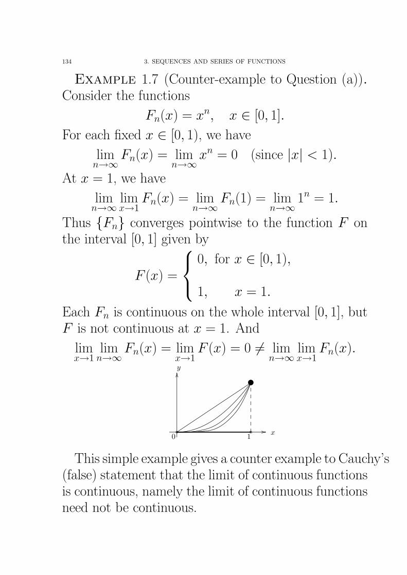
134 3. SEQUENCES AND SERIES OF FUNCTIONS
Example 1.7 (Counter-example to Question (a)).Consider the functions
Fn(x) = xn, x ∈ [0, 1].
For each fixed x ∈ [0, 1), we have
limn→∞
Fn(x) = limn→∞
xn = 0 (since |x| < 1).
At x = 1, we have
limn→∞
limx→1
Fn(x) = limn→∞
Fn(1) = limn→∞
1n = 1.
Thus {Fn} converges pointwise to the function F onthe interval [0, 1] given by
F (x) =
0, for x ∈ [0, 1),
1, x = 1.
Each Fn is continuous on the whole interval [0, 1], butF is not continuous at x = 1. And
limx→1
limn→∞
Fn(x) = limx→1
F (x) = 0 6= limn→∞
limx→1
Fn(x).
................................................................................................................................................................................................................................................................................................................................................................................. ................
........
........
........
........
........
........
........
........
........
........
........
........
........
........
........
........
........
........
........
........
........
........
........
........
........
........
........
........
........
...................
................
0 1 x
y
......................................................................................................................................................................................................................................................................................................................................
................................................................................................................................................................................................................................................................................................................................................................................................................................................................................................................................................................................................................................................................................................................................................................................................................................................
•
.....................................................................................................................
........................................
...............................
....................................................................................................................................................................................................
.........................................................................................................................
...................................
...................................................................................................................................................................................................
......................................................................................................................................................
....................................................................................................................................................................................................................
........
.....
........
.....
........
.....
........
.....
........
.....
........
.....
........
.....
......
This simple example gives a counter example to Cauchy’s(false) statement that the limit of continuous functionsis continuous, namely the limit of continuous functionsneed not be continuous.
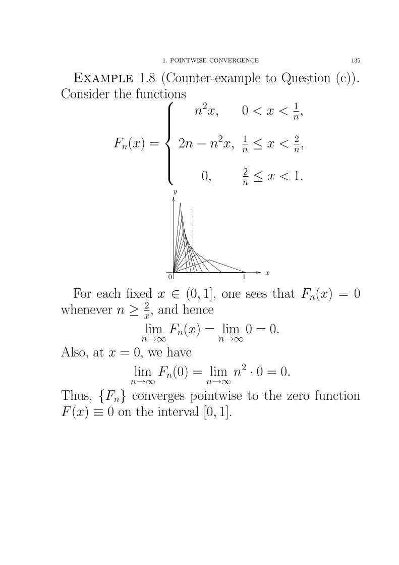
1. POINTWISE CONVERGENCE 135
Example 1.8 (Counter-example to Question (c)).Consider the functions
Fn(x) =
n2x, 0 < x < 1
n,
2n− n2x, 1n ≤ x < 2
n,
0, 2n ≤ x < 1.
................................................................................................................................................................................................................................................................................................................................................................................. ................
........
........
........
........
........
........
........
........
........
........
........
........
........
........
........
........
........
........
........
........
........
........
........
........
........
........
........
........
........
........
........
........
........
........
........
........
........
........
..................
................
0 1 x
y
................................................
................................................
.............................................................................................................................................................................................................
...................................................................................................................................................................................................................................
.......................................................................................................................................................................................................................................
...................................................................................................................................................................................................................................................................
.........................................................................................................................................................................................................................................................................................................
....................................................................................................................................................................................................................................................................................................................................................
........
........
........
........
........
........
........
........
........
........
........
........
........
........
........
........
........
........
........
........
........
........
........
........
........
............................................................................................................................................................................................................................................................................................................................................................................................................................................................................................................................................................................................................................................................................................................................................................................................................................................................................................................................................................................................................................................................................................................................................................................................................................................................................................................................................................................................................................................................................................................................................................................................................................
.....
........
.....
........
.....
........
.....
........
.....
........
.....
........
.....
........
.....
........
.....
........
..
For each fixed x ∈ (0, 1], one sees that Fn(x) = 0whenever n ≥ 2
x, and hence
limn→∞
Fn(x) = limn→∞
0 = 0.
Also, at x = 0, we have
limn→∞
Fn(0) = limn→∞
n2 · 0 = 0.
Thus, {Fn} converges pointwise to the zero functionF (x) ≡ 0 on the interval [0, 1].
136 3. SEQUENCES AND SERIES OF FUNCTIONS
For each n ≥ 1, we have∫ 1
0
Fn(x) dx =
∫ 1/n
0
n2x dx+
∫ 2/n
1/n
(2n−n2x) dx+
∫ 1
2/n
0 dx
=n2x2
2
∣∣∣∣ 1n0
+
(2nx− n2x2
2
)∣∣∣∣ 2n1n
+ 0
=1
2+ (4− 2)− (2− 1
2) + 0 = 1.
Thus we have
limn→∞
∫ 1
0
Fn(x) dx = limn→∞
1 = 1 6= 0 =
∫ 1
0
F (x) dx, i.e.
limn→∞
∫ 1
0
Fn(x) dx 6=∫ 1
0
(lim
n→∞Fn(x)
)dx.
Reason: At different x, Fn(x) converges to F (x)at different pace (more specifically, in the definitionof pointwise convergence, the choice of N depends onboth ε and x).
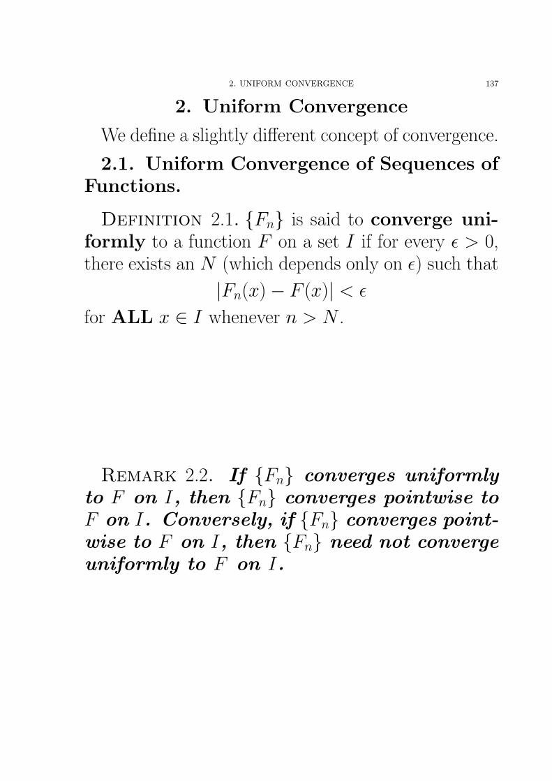
2. UNIFORM CONVERGENCE 137
2. Uniform Convergence
We define a slightly different concept of convergence.
2.1. Uniform Convergence of Sequences ofFunctions.
Definition 2.1. {Fn} is said to converge uni-formly to a function F on a set I if for every ε > 0,there exists an N (which depends only on ε) such that
|Fn(x)− F (x)| < ε
for ALL x ∈ I whenever n > N .
Remark 2.2. If {Fn} converges uniformlyto F on I, then {Fn} converges pointwise toF on I. Conversely, if {Fn} converges point-wise to F on I, then {Fn} need not convergeuniformly to F on I.
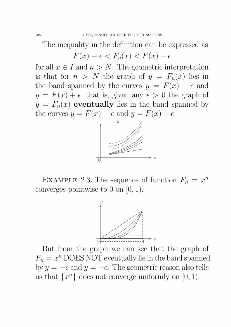
138 3. SEQUENCES AND SERIES OF FUNCTIONS
The inequality in the definition can be expressed as
F (x)− ε < Fn(x) < F (x) + ε
for all x ∈ I and n > N . The geometric interpretationis that for n > N the graph of y = Fn(x) lies inthe band spanned by the curves y = F (x) − ε andy = F (x) + ε, that is, given any ε > 0 the graph ofy = Fn(x) eventually lies in the band spanned bythe curves y = F (x)− ε and y = F (x) + ε.
................................................................................................................................................................................................................................................................................................................................................................................. ................
........
........
........
........
........
........
........
........
........
........
........
........
........
........
........
........
........
........
........
........
........
........
........
........
........
........
........
........
........
...................
................
0 x
y
..............................................................................................
..............................................................................................
...................................................................................
........................................
...................................................................................................................................................................................
................................................................................
...............................................
......................................
.................................
...............................
.....
.................................................................
.............................................
.....................................
.................................
..............................
.............................
.......................................................
..........................................
...................................
..............................
...............................
...........................................................
.............................................
.....................
..................
........................
......................................................
.............................................
.....................
..................
........................
......................................................
Example 2.3. The sequence of function Fn = xn
converges pointwise to 0 on [0, 1).
................................................................................................................................................................................................................................................................................................................................................................................. ................
........
........
........
........
........
........
........
........
........
........
........
........
........
........
........
........
........
........
........
........
........
........
........
........
........
........
........
........
........
........
........
.....................
................
0 1 x
y
......................................................................................................................................................................................................................................................................................................................................
.....................................................................................................................................................................................................................................................................................................................................................................................................................................................................................................................................................................................................................................................................................................................................................................................................................................................................................................................................................................
........................................
...............................
....................................................................................................................................................................................................
.........................................................................................................................
...................................
...................................................................................................................................................................................................
......................................................................................................................................................
....................................................................................................................................................................................................................
........
........
........
........
........
........
........
........
........
........
........
........
.
........ ........ ........ ........ ........ ........ ........ ........ ........ ........ ........ ........ ........ ........ ........ ........ ........ ........ ..
........ ........ ........ ........ ........ ........ ........ ........ ........ ........ ........ ........ ........ ........ ........ ........ ........ ........ ..
But from the graph we can see that the graph ofFn = xn DOES NOT eventually lie in the band spannedby y = −ε and y = +ε. The geometric reason also tellsus that {xn} does not converge uniformly on [0, 1).
2. UNIFORM CONVERGENCE 139
2.2. Two Criteria for Uniform Convergenceof {Fn}. The following theorem is useful (computa-tionally) in determining whether a sequence of func-tions converges uniformly or not.
Theorem 2.4 (T -test). Suppose {Fn} is a sequenceof functions converging pointwise to a function Fon a set I, and let
Tn = supx∈I
|Fn(x)− F (x)|.
Then {Fn} converges uniformly to F on I ifand only if lim
n→∞Tn = 0.
140 3. SEQUENCES AND SERIES OF FUNCTIONS
Proof. First we prove the ‘only if’ part. Supposethat {Fn} converges uniformly to F on I . Then forany given ε > 0, there exists N such that
|Fn(x)− F (x)| < ε
2for all n > N and x ∈ I
=⇒ Tn = supx∈I
|Fn(x)−F (x)| ≤ ε
2< ε for all n > N
=⇒ |Tn − 0| = Tn < ε for all n > N.
Hence we have limn→∞
Tn = 0.
Next we prove the ‘if’ part. Suppose that limn→∞
Tn =
0.
Then for any given ε > 0, there exists N such that
|Tn − 0| = Tn < ε for all n > N
=⇒ supx∈I
|Fn(x)− F (x)| < ε for all n > N
=⇒ |Fn(x)− F (x)| < ε for all n > N and x ∈ I.
Hence {Fn} converges uniformly to F on I . Thisfinishes the proof of the theorem. �
2. UNIFORM CONVERGENCE 141
Theorem 2.5 (Cauchy’s Criterion). A sequenceof functions {Fn} converges uniformly on aset I if and only if given any ε > 0, thereexists a natural number N such that(5)|Fn(x)−Fm(x)| < ε for all x ∈ I and all m, n > N.
Remark: Here N does not depend on x.
142 3. SEQUENCES AND SERIES OF FUNCTIONS
Proof. First we prove the ‘only if’ part. Supposethat {Fn} converges uniformly to the function F on I .
Then given any ε > 0, there exists N such that
|Fn(x)− F (x)| < ε
2for all x ∈ I and all n > N.
Then for all x ∈ I and m, n > N ,
|Fn(x)−Fm(x)| = |(Fn(x)−F (x))− (Fm(x)−F (x))|≤ |Fn(x)− F (x)| + |Fm(x)− F (x)| < ε
2+
ε
2= ε.
This finishes the proof of the ‘only if’ part.
Next we prove the ‘if’ part. Suppose that equation 5holds.
Then for each fixed point x ∈ I , {Fn(x)} is a Cauchysequence of real numbers, and thus by Cauchy’s crite-rion for sequences, the sequence of real numbers {Fn(x)}converges.
For each x ∈ I , we denote the limit by F (x) =lim
n→∞Fn(x). Then {F (x)}x∈I forms a function on I ,
which we denote by F .
Given any ε > 0, by equation 5, there exists N suchthat
|Fn(x)−Fm(x)| < ε
2for all x ∈ I and all m, n > N.
2. UNIFORM CONVERGENCE 143
Then for each fixed x ∈ I and n > N , we have
|Fn(x)− F (x)| = |Fn(x)− limm→∞
Fm(x)|
= limm→∞
|Fn(x)− Fm(x)| ≤ limm→∞
ε
2=
ε
2< ε.
Thus {Fn} converges uniformly to F , and this fin-ishes the proof of the ‘if’ part. �
144 3. SEQUENCES AND SERIES OF FUNCTIONS
2.3. Examples.
Example 2.6. Show that Fn(x) =sin2 x
n, x ∈
(−∞, +∞), converges uniformly.
Proof. The limiting function F (x) is
F (x) = limn→∞
sin2 x
n= 0
for all x ∈ (−∞, +∞). Since
Tn = supx∈(−∞,+∞)
|Fn(x)− F (x)|
= supx∈(−∞,+∞)
∣∣∣∣sin2 x
n
∣∣∣∣ ≤ 1
n→ 0
as n → ∞, thus the sequence of functions {Fn(x}converges uniformly on (−∞, +∞). �
2. UNIFORM CONVERGENCE 145
Example 2.7. Determine whether the followingsequences of functions converge uniformly on theindicated interval.
(a) fn(x) =n2 ln x
xn, x ∈ [1, +∞);
(b) fn(x) =n2 ln x
xn, x ∈ [2, +∞).
146 3. SEQUENCES AND SERIES OF FUNCTIONS
Solution. Let f (x) = limn→∞
fn(x) = 0 for x ≥ 1.
(a). Tn = supx≥1
|fn(x)− 0| = supx≥1
n2 ln x
xn= sup
x≥1fn(x).
From
f ′n(x) = n21
x·x−n−n3 ln x·x−n−1 =
n2 − n3 ln x
xn+1= 0,
we have n2−n3 ln x = 0 or x = e1n . Observe that fn(x)
is monotone increasing for 1 ≤ x ≤ e1n and monotone
decreasing for x ≥ e1n . Thus
Tn = maxx≥1
fn(x) = fn(e1n) =
n2 · 1n(
e1n
)n =n
e6→ 0
as n → ∞ and so {fn(x)} does NOT converge uni-formly.
(b). Since e1n ≤ 2 for n ≥ 2, the function fn(x)
is monotone decreasing on [2, +∞) for n ≥ 2 and so
Tn = supx≥2
|fn(x) − f (x)| = fn(2) =n2 ln 2
2nfor n ≥
2. Since limn→∞
Tn = 0, {fn} converges uniformly on
[2, +∞). �
2. UNIFORM CONVERGENCE 147
Example 2.8. Show that Fn(x) =n2 ln x sin nx
xn
converges uniformly on [2, +∞).
Solution. F (x) = limn→∞
Fn(x) = 0 for x ≥ 2. Ob-serve
Tn = supx≥2
|Fn(x)−F (x)| = supx≥2
n2 ln x| sin nx|xn
≤ n2 ln 2
2n
for n ≥ 2. Since limn→∞
Tn = 0, {Fn} converges uni-
formly. �
Remark. Let {Fn} be a sequence of functions on aninterval I . To see whether {Fn} is uniformly conver-gent, we may try to do by the following steps.
(1). Determine the limiting function F (x) = limn→∞
Fn(x).
(2). Determine Tn = supx∈I
|Fn(x)− F (x)|.
(3). Check whether limn→∞
Tn = 0.
If Tn is difficult to be determined, then we may try toestimate an upper bound of Tn ( a lower bound of Tn
if we guess that the sequence of functions might not beuniformly convergent).
148 3. SEQUENCES AND SERIES OF FUNCTIONS
2.4. Uniform Convergence of Series of Func-tions.
Definition 2.9.∞∑
n=1
fn is said to converge uni-
formly (to S) on I if the sequence of its partial sums{Sn} converges uniformly (to S) on I .
Theorem 2.10 (T -test for Series of Functions).
Suppose∞∑
n=1
fn(x) is a series of functions converg-
ing pointwise on a set I, and let
Tn = supx∈I
∣∣∣∣∣∞∑
k=n+1
fk(x)
∣∣∣∣∣ .Then
∞∑n=1
fn(x) converges uniformly on I if
and only if limn→∞
Tn = 0.
Proof. Let Sn(x) =
n∑k=1
fk(x) and S(x) =
∞∑k=1
fk(x).
Then
|Sn(x)− S(x)| =
∣∣∣∣∣∞∑
k=n+1
fk(x)
∣∣∣∣∣and so the T -test, Theorem 2.4, applies. �
2. UNIFORM CONVERGENCE 149
Theorem 2.11 (Cauchy Criterion). A series of
functions∞∑
n=1
fn converges uniformly on a
set I if and only if given any ε > 0, thereexists a natural number N such that∣∣∣∣∣
m∑k=n+1
fk(x)
∣∣∣∣∣ < ε for all x ∈ I and all m > n > N.
Remark: Here N does not depend on x.
Proof. The proof follows by applying the Cauchy
Criterion to the partial sums Sn(x) =
n∑k=1
fk(x). �
150 3. SEQUENCES AND SERIES OF FUNCTIONS
The following test is very useful in verifying thatcertain series of functions converge uniformly to somefunctions on an interval.
Theorem 2.12 (Weierstrass M -test). Consider
a series of functions∞∑
k=1
fk on a set I. Sup-
pose that
(i) |fk(x)| ≤ Mk for all x ∈ I, k = 1, 2, · · · ,and
(ii)∞∑
k=1
Mk converges.
Then∞∑
k=1
fk converges uniformly (to some
function) on I.
Remark. Weierstrass M -test only states that if aseries of functions satisfies conditions (i) and (ii), itconverges uniformly on I . If a series of functions doesnot satisfy these two conditions, the test fails, namely,no conclusion that you can claim from this test.
2. UNIFORM CONVERGENCE 151
Proof. Since
∞∑k=1
Mk converges (by (ii)), by the
Cauchy Criterion, given any ε > 0, there exists Nsuch that
m∑k=n+1
Mk =
∣∣∣∣∣m∑
k=n+1
Mk
∣∣∣∣∣ < ε for all m > n > N
because Mk ≥ 0.
Then for all x ∈ I , we have∣∣∣∣∣m∑
k=n+1
fk(x)
∣∣∣∣∣ ≤m∑
k=n+1
|fk(x)| ≤m∑
k=n+1
Mk < ε.
Thus, by the Cauchy criterion,
∞∑k=1
fk converges uni-
formly on I . �
152 3. SEQUENCES AND SERIES OF FUNCTIONS
2.5. Examples.
Example 2.13. Show that∞∑
n=1
cosn x
n2 + xconverges
uniformly on (0,∞).
Proof. Since ∣∣∣∣ cosn x
n2 + x
∣∣∣∣ ≤ 1
n2
for all x ∈ (0,∞) and the series
∞∑n=1
1
n2is convergent
by the p-series, the series of functions
∞∑n=1
cosn x
n2 + xcon-
verges uniformly by the Weierstrass M -test and hencethe result. �
2. UNIFORM CONVERGENCE 153
Example 2.14. Does the series of functions∞∑
n=1
n2xn sin nx
converge uniformly on the interval [0, 12]? Justify
your answer.
Solution. Note that∣∣∣n2xn sin nx∣∣∣ ≤ n2
2n
for x ∈ [0, 12]. Since
limn→∞
(n + 1)2
2n+1
n2
2n
= limn→∞
(n + 1)2
2n2=
1
2< 1,
the series
∞∑n=1
n2
2nconverges, by the ratio test,
and so the series of functions∞∑
n=1
n2xn sin nx
converges uniformly on [0, 12] by the Weierstrass M -
test. �
154 3. SEQUENCES AND SERIES OF FUNCTIONS
Example 2.15. Show that the series∞∑
n=1
(−1)n+1xn
n
converges uniformly on [0, 1].
Note. The M -test fails for this example because
supx∈[0,1]
∣∣∣∣(−1)n+1xn
n
∣∣∣∣ =1
n
and
∞∑n=1
1
ndiverges. In this case, we use T -test or
Cauchy Criterion.
Proof. Let an(x) =xn
n. Then, for 0 ≤ x ≤ 1, we
have
a1(x) ≥ a2(x) ≥ · · · ≥ 0 and limn→∞
an(x) = 0.
Thus the series
∞∑n=1
(−1)n+1xn
nconverges pointwise on
[0, 1] by the Alternating Series Test.
By the Alternating Series Estimation,
Tn = sup0≤x≤1
∣∣∣∣∣∞∑
k=n+1
(−1)k+1xk
k
∣∣∣∣∣ ≤ sup0≤x≤1
xn+1
n + 1=
1
n + 1.
Since limn→∞
1
n + 1= 0, the series (−1)n+1x
n
nconverges
uniformly by the T -test. �
2. UNIFORM CONVERGENCE 155
Example 2.16. Show that the series∞∑
n=1
xn
ndoes
not converge uniformly on [0, 1).
Proof. Observe that
Tn = sup0≤x<1
|Sn(x)− S(x)| = sup0≤x<1
∣∣∣∣∣∞∑
k=n+1
xk
k
∣∣∣∣∣= sup
0<x<1
∞∑k=n+1
xk
k.
= sup0<x<1
(xn+1
n + 1+
xn+2
n + 2+ · · ·
)≥ sup
0<x<1
(xn+1
n + 1+
xn+2
n + 2+ · · · + x2n
2n
)=
1
n + 1+
1
n + 2+ · · · + 1
2n
(becausexk
kmonotone increasing on (0, 1))
≥ 1
2n+
1
2n+ · · · + 1
2n= n · 1
2n=
1
2.
Thus the sequence {Tn} does not tend to 0 and so
the series of functions
∞∑k=1
xk
kdoes NOT converge uni-
formly on [0, 1) by the T -test. �
156 3. SEQUENCES AND SERIES OF FUNCTIONS
3. Uniform Convergence of {Fn} andContinuity
In this section we will prove that the limit of uni-formly convergent sequence of continuous functions isagain continuous.
Theorem 3.1.Let {Fn} be a sequence of con-tinuous functions on an interval I. Supposethat {Fn} converges uniformly to a functionF on I. Then F is continuous on I.
Proof. Fix any point x0 ∈ I . We are going toshow that F is continuous at the point x0.
Given any ε > 0, since {Fn} converges uniformly toF on I , there exists N such that
|Fn(x)− F (x)| < ε
3for all x ∈ I and all n > N.
Next we fix an n > N (say, n = [N ] + 1). Since Fn
is continuous at x0, there exists δ > 0 (here δ dependson x0 and ε) such that for all x satisfying |x−x0| < δ,we have
|Fn(x)− Fn(x0)| <ε
3.
Then for all x satisfying |x− x0| < δ, we have
|F (x)− F (x0)|= |F (x)−Fn(x) + Fn(x)−Fn(x0) + Fn(x0)−F (x0)|≤ |F (x)−Fn(x)|+|Fn(x)−Fn(x0)|+|Fn(x0)−F (x0)|
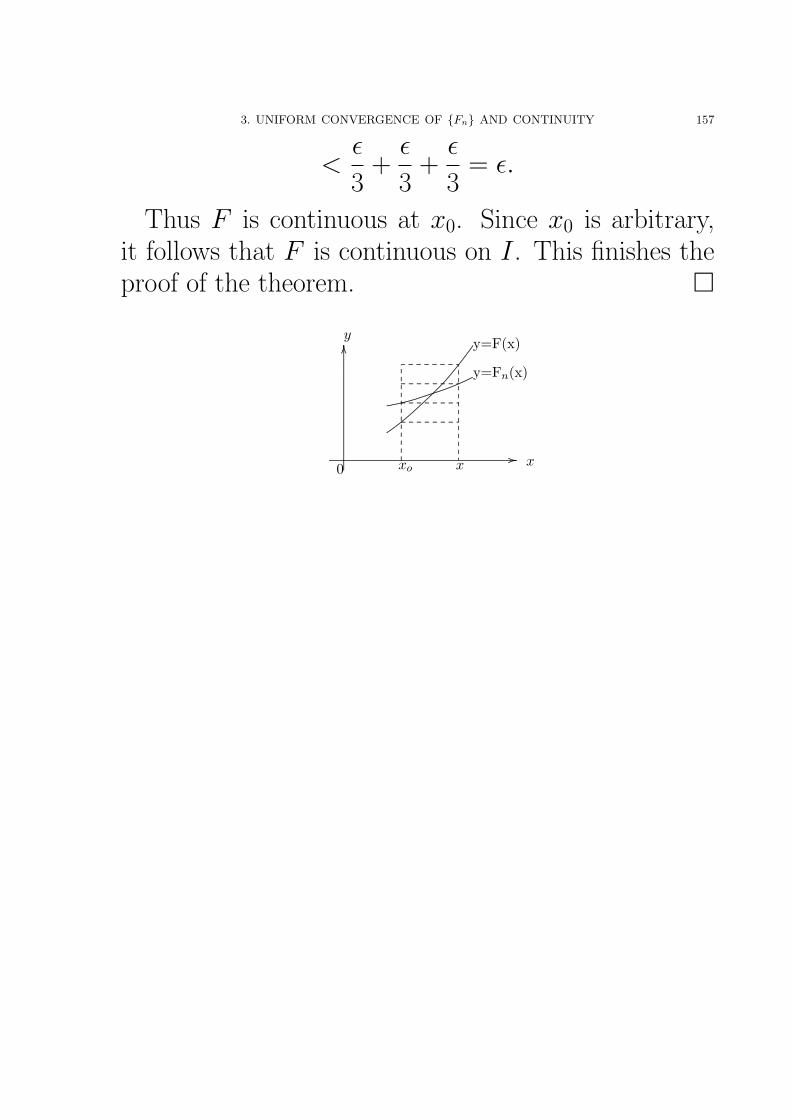
3. UNIFORM CONVERGENCE OF {Fn} AND CONTINUITY 157
<ε
3+
ε
3+
ε
3= ε.
Thus F is continuous at x0. Since x0 is arbitrary,it follows that F is continuous on I . This finishes theproof of the theorem. �
................................................................................................................................................................................................................................................................................................................................................................................. ................
........
........
........
........
........
........
........
........
........
........
........
........
........
........
........
........
........
........
........
........
........
........
........
........
........
........
........
........
........
...................
................
0 xxo x
y=F(x)
y=Fn(x)
y
.........................................................................................................................................................................................................................................
................................................................
..................................................
........................................
..................
........
........
........
........
........
........
........
........
........
........
........
........
........ ........ ........ ........ ........ ........ ........ .....................................................................................................
........ ........ ........ ........ ........ ........ ........ ....
........ ........ ........ ........ ........ ........ ........ ....
........ ........ ........ ........ ........ ........ ........ ....
158 3. SEQUENCES AND SERIES OF FUNCTIONS
Example 3.2. Find the pointwise limit F of thesequence
Fn(x) =x2n
1 + x2n, x ∈ [0, 1].
Show using Theorem 3.1 that the convergence is notuniform.
Solution. If 0 ≤ x < 1, we have
limn→∞
Fn(x) = limn→∞
x2n
1 + x2n=
0
1 + 0= 0.
If x = 1, then Fn(1) =1
2. Thus the limiting function
F (x) is
F (x) =
0 0 ≤ x < 1
12 x = 1
Because each Fn(x) is continuous but F (x) is not, thesequence of functions {Fn(x)} does not converge uni-formly on [0, 1] by Theorem 3.1. �
3. UNIFORM CONVERGENCE OF {Fn} AND CONTINUITY 159
It is possible that each Fn and F (x) = limn→∞
Fn(x)
are continuous on an interval I , but {Fn} does notconverge uniformly to F (x).
For the case that I is not closed, an example canbe given by I = [0, 1), Fn(x) = xn. (In this caseF (x) = lim
n→∞Fn(x) = 0 for x ∈ I .)
For the case that I is a closed interval, an examplecan be given as follows.
160 3. SEQUENCES AND SERIES OF FUNCTIONS
Example 3.3. Let Fn(x) = nxe−nx2. Show that
1) Each Fn(x) is continuous on I = [0, 1].2) {Fn(x)} converges pointwise to a continuous
function on I.3) {Fn(x)} does not converge uniformly on I.
Proof. Each Fn(x) is continuous because it is awell-defined elementary function on [0, 1].
Let F (x) = limn→∞
Fn(x) on [0, 1]. When x = 0,
Fn(0) = 0 for each n and F (0) = limn→∞
0 = 0, when
x 6= 0 (fixed),
F (x) = limn→∞
Fn(x) = limn→∞
nxe−nx2= lim
n→∞
nx
enx2
= limn→∞
x
enx2 · x2= lim
n→∞
1
xenx2 = 0.
Thus F (x) = 0 is continuous on [0, 1].Now Tn = sup
0≤x≤1|Fn(x)− F (x)| = sup
0≤x≤1Fn(x). From
F ′n(x) = ne−nx2
+ nxe−nx2 · (−2nx)
= ne−nx2(1− 2nx2) = 0,
we have x = ±√
1
2n. Since Fn(0) = 0 and Fn(1) =
ne−n,
sup0≤x≤1
Fn(x) = max0≤x≤1
Fn(x)
3. UNIFORM CONVERGENCE OF {Fn} AND CONTINUITY 161
= max
{0,
n
en, n · 1√
2n· e−n· 1
2n
}=
√n
2e.
Thus Tn =
√n
2e. Since lim
n→∞Tn = +∞, the sequence
{Fn} does not converge uniformly to F (x) on [0, 1].�
162 3. SEQUENCES AND SERIES OF FUNCTIONS
Corollary 3.4. Suppose that∞∑
k=1
fk con-
verges uniformly to a function S on an in-terval I. Suppose that each fk is continuouson I. Then S is also continuous on I.
Proof. Consider the sequence of partial sums {Sn}
on I , where we have Sn =
n∑k=1
fk. Then {Sn} con-
verges uniformly to S on I . If each fk is continuouson I , then each Sn is also continuous on I . Then byTheorem 3.1, S is also continuous on I . �
3. UNIFORM CONVERGENCE OF {Fn} AND CONTINUITY 163
Example 3.5. Is∞∑
n=1
x
n2enx, x ∈ (0,∞), a con-
tinuous function?
Solution. Let fn(x) =x
n2enx.
We find an upper bound of fn(x). Observe that
f ′n(x) =( x
n2enx
)′=
(xe−nx
n2
)′=
e−nx − nxe−nx
n2
=
e−nx
(1
n− x
)n
.
Thus f ′n(x) > 0 for 0 < x < 1n and f ′n(x) < 0 for
x > 1n. It follows that fn(x) is monotone increasing on
(0, 1n] and monotone decreasing on [1n, +∞). Hence
sup0<x<+∞
fn(x) = max0<x<+∞
fn(x) = fn
(1
n
)=
1n
n2en· 1n=
1
en3.
Let Mn =1
en3. Then |fn(x)| ≤ Mn for x ∈ (0,∞).
Since
∞∑n=1
Mn converges by the p-series, the series of
164 3. SEQUENCES AND SERIES OF FUNCTIONS
functions
∞∑n=1
x
n2enxconverges uniformly by Weierstrass
M -test on (0,∞).
According to Corollary 3.4, the function
∞∑n=1
x
n2enx
is continuous on (0,∞). �
3. UNIFORM CONVERGENCE OF {Fn} AND CONTINUITY 165
It is possible that each fn and
∞∑n=1
fn are continuous,
but
∞∑n=1
fn does not converge uniformly.
Example 3.6. Consider the geometric series∞∑
n=0
xn = 1 + x + x2 + · · · =1
1− x
for −1 < x < 1. In this case, each xn and
∞∑n=0
xn are
continuous on I = (−1, 1). We show that
∞∑n=0
xn does
not converge uniformly by T -test.
Since
Tn = sup−1<x<1
∣∣xn+1 + xn+2 + · · ·∣∣
≥ sup0≤x<1
∣∣xn+1 + xn+2 + · · ·∣∣
= sup0≤x<1
(xn+1 + xn+2 + · · ·
)≥ sup
0≤x<1xn+1 = 1,
the sequence {Tn} does not tend to 0
and so the series
∞∑n=0
xn does not converge uniformly
on (−1, 1) by the T -test. �
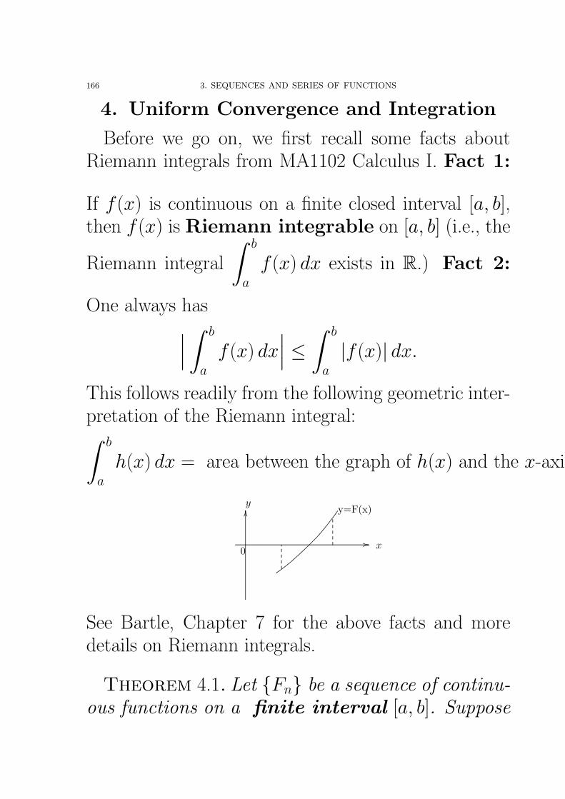
166 3. SEQUENCES AND SERIES OF FUNCTIONS
4. Uniform Convergence and Integration
Before we go on, we first recall some facts aboutRiemann integrals from MA1102 Calculus I. Fact 1:
If f (x) is continuous on a finite closed interval [a, b],then f (x) is Riemann integrable on [a, b] (i.e., the
Riemann integral
∫ b
a
f (x) dx exists in R.) Fact 2:
One always has∣∣∣ ∫ b
a
f (x) dx∣∣∣ ≤ ∫ b
a
|f (x)| dx.
This follows readily from the following geometric inter-pretation of the Riemann integral:∫ b
a
h(x) dx = area between the graph of h(x) and the x-axis along [a,b].
................................................................................................................................................................................................................................................................................................................................................................................. ................
........
........
........
........
........
........
........
........
........
........
........
........
........
........
........
........
........
........
........
........
........
........
........
........
........
........
........
........
........
...................
................
0 x
y=F(x)y
.........................................................................................................................................................................................................................................
........
........
........
........
.... ........................................
See Bartle, Chapter 7 for the above facts and moredetails on Riemann integrals.
Theorem 4.1. Let {Fn} be a sequence of continu-ous functions on a finite interval [a, b]. Suppose
4. UNIFORM CONVERGENCE AND INTEGRATION 167
that {Fn} converges uniformly on [a, b]. Then
limn→∞
∫ b
a
Fn(x) dx =
∫ b
a
(lim
n→∞Fn(x)
)dx.
Proof. Let F (x) = limn→∞
Fn(x). Since each Fn(x)
is continuous and Fn(x) converges uniformly on [a, b],the function F (x) is continuous on [a, b] and the inte-
gral∫ b
a F (x) dx exists.By definition, given any ε > 0, there exists N such
that
|Fn(x)− F (x)| < ε
2(b− a)
for all n > N and x ∈ [a, b]. Thus
Fn(x)− ε
2(b− a)< F (x) < Fn(x) +
ε
2(b− a)
for all x ∈ [a, b] and n > N .
It follows that, for n > N ,∫ b
a
(Fn(x)− ε
2(b− a)
)dx ≤
∫ b
a
F (x) dx
≤∫ b
a
(Fn(x) +
ε
2(b− a)
)dx
and so∫ b
a
Fn(x) dx− ε
2≤∫ b
a
F (x) dx ≤∫ b
a
Fn(x) dx +ε
2
168 3. SEQUENCES AND SERIES OF FUNCTIONS
or ∣∣∣∣∣∫ b
a
Fn(x) dx−∫ b
a
F (x) dx
∣∣∣∣∣ ≤ ε
2< ε.
Thus
limn→∞
∫ b
a
Fn(x) dx =
∫ b
a
F (x) =
∫ b
a
limn→∞
Fn(x) dx,
which is the assertion.�
4. UNIFORM CONVERGENCE AND INTEGRATION 169
Example 4.2. Compute, justifying your answer,
limn→∞
∫ 1
0
sin nx
n + x2dx.
Solution. Let Fn(x) =sin nx
n + x2. Then the limiting
function
F (x) = limn→∞
Fn(x) = limn→∞
sin nx
n + x2= 0
for any given 0 ≤ x ≤ 1, by the Squeeze theorem,because
−1
n≤ sin nx
n + x2≤ 1
n
and limn→∞
1
n= − lim
n→∞
1
n= 0. Since
Tn = sup0≤x≤1
|Fn(x)− F (x)| = sup0≤x≤1
∣∣∣∣ sin nx
n + x2
∣∣∣∣ ≤ 1
n,
limn→∞
Tn = 0 by the Squeeze Theorem and so the se-
quence of functions {Fn} converges uniformly to F (x).Thus
limn→∞
∫ 1
0
sin nx
n + x2dx =
∫ 1
0
limn→∞
sin nx
n + x2dx =
∫ 1
0
0 dx = 0.
�
170 3. SEQUENCES AND SERIES OF FUNCTIONS
Corollary 4.3. Suppose that∞∑
k=1
fk converges
uniformly on a finite interval [a, b] such thateach fk is continuous on [a, b]. Then∫ b
a
∞∑k=1
fk(x) dx =
∞∑k=1
∫ b
a
fk(x) dx.
Proof. By definition, the sequence of partial sums
Sn =n∑
k=1
fk converges uniformly on [a, b]. Since each
fk is continuous on [a, b], then each partial sum Sn isalso continuous on [a, b]. Thus∫ b
a
∞∑k=1
fk dx =
∫ b
a
limn→∞
Sn(x) dx
= limn→∞
∫ b
a
Sn(x) dx = limn→∞
∫ b
a
n∑k=1
fk(x) dx
= limn→∞
n∑k=1
∫ b
a
fk(x) dx =
∞∑k=1
∫ b
a
fk(x) dx.
�
4. UNIFORM CONVERGENCE AND INTEGRATION 171
By using this theorem, we have the following amaz-ing formula.
Example 4.4. Show that
ln 2 =
∞∑n=1
1
n · 2n=
1
2+
1
2 · 22+
1
3 · 23+ · · ·
Proof. Since∣∣xn−1
∣∣ ≤ (1
2
)n−1
for 0 ≤ x ≤ 1
2and
the geometric series
∞∑n=0
(1
2
)n−1
converges, the series
∞∑n=1
xn−1 converges uniformly to1
1− xon [0, 1
2] by the
Weierstrass M -test. Thus we have∫ 12
0
1
1− x=
∫ 12
0
∞∑n=1
xn−1 dx
=
∞∑n=1
∫ 12
0
xn−1 dx =
∞∑n=1
xn
n
∣∣∣∣1/20
=
∞∑n=1
1
n · 2n.
Since∫ 12
0
1
1− x= − ln(1− x)
∣∣∣120
= − ln
(1− 1
2
)= − ln
(1
2
)= ln 2,
172 3. SEQUENCES AND SERIES OF FUNCTIONS
we obtain the formula
ln 2 =
∞∑n=1
1
n · 2n=
1
2+
1
2 · 22+
1
3 · 23+ · · · .
�
Remark 4.5. Example 4.4 gives a way to estimatethe number ln 2 because the remainder
Rn =
∞∑k=n+1
1
k · 2k=
1
(n + 1)2n+1+
1
(n + 2)2n+2+ · · ·
<1
(n + 1)2n+1+
1
(n + 1)2n+2+
1
(n + 1)2n+3+ · · ·
=1
(n + 1)2n+1
(1 +
1
2+
1
22+ · · ·
)=
1
(n + 1)2n+1· 1
1− 12
=1
(n + 1)2n.
For instance,
ln 2 ≈ 1
2+
1
2 · 22+
1
3 · 23+ · · · + 1
10 · 210
with error less than1
11 · 210=
1
11264.
5. UNIFORM CONVERGENCE AND DIFFERENTIATION 173
5. Uniform Convergence andDifferentiation
Theorem 5.1. Let {Fn} be a sequence of func-tions on [a, b] such that
(i) each F ′n exists and is continuous on [a, b],
(ii) {Fn} converges pointwise to a function Fon [a, b], and
(iii) {F ′n} converges uniformly on [a, b].
Then F is differentiable on [a, b], and for allx ∈ [a, b],
F ′(x) = limn→∞
F ′n(x),
i.e.d
dx
(lim
n→∞Fn(x)
)= lim
n→∞
(d
dxFn(x)
).
Remark. Here the differentiability and continuity atthe endpoints a and b refer to the one sided derivativesand limits respectively.
174 3. SEQUENCES AND SERIES OF FUNCTIONS
Proof. By (iii), {F ′n} converges uniformly to a func-
tion, denoted by g, on [a, b], where
g(x) = limn→∞
F ′n(x)
for all x ∈ [a, b].
By (i), since each F ′n is continuous on [a, b], F ′
n is alsoRiemann integrable on [a, b], and by the fundamentaltheorem of calculus,∫ x
a
F ′n(t) dt = Fn(x)− Fn(a) for all x ∈ [a, b].
Letting n →∞, for all x ∈ [a, b],
limn→∞
∫ x
a
F ′n(t) dt = lim
n→∞
(Fn(x)−Fn(a)
)= F (x)−F (a)
========================F ′nuniform convergence on[a,x]⊆[a,b]
∫ x
a
limn→∞
F ′n(t) dt =
∫ x
a
g(t) dt.
Thus
F (x) = F (a) +
∫ x
a
g(t) dt
and so
F ′(x) =d
dx
∫ x
a
g(t) dt = g(x)
by the fundamental theorem of calculus. In other words
d
dx
(lim
n→∞Fn(x)
)= lim
n→∞
(d
dxFn(x)
)and hence the result. �
5. UNIFORM CONVERGENCE AND DIFFERENTIATION 175
Remark 5.2. By inspecting the proof, Theorem 5.1still holds when the closed interval [a, b] is replacedby (a, b), (a, b] or [a, b).
Corollary 5.3. Let∞∑
k=1
fk be a series of func-
tions on [a, b] such that
(i) each f ′k exists and continuous on [a, b],
(ii)
∞∑k=1
fk converges pointwise on [a, b], and
(iii)
∞∑k=1
f ′k converges uniformly on [a, b].
Thend
dx
( ∞∑k=1
fk(x)
)=
∞∑k=1
d
dxfk(x).
Proof.
d
dx
( ∞∑k=1
fk(x)
)=
d
dxlim
n→∞
n∑k=1
fk(x)
================check conditions (i)-(iii)
limn→∞
d
dx
(n∑
k=1
fk(x)
)
= limn→∞
n∑k=1
f ′k(x) =
∞∑k=1
d
dxfk(x).
�
176 3. SEQUENCES AND SERIES OF FUNCTIONS
Example. Let S(x) =∞∑
k=1
sin kx2k . Let fk(x) = sin kx
2k .
Then
(i) each f ′k exists and continuous on R.
(ii)∞∑
k=1
fk converges pointwise on R because
|fk(x)| ≤ 1
2k
and∞∑
k=1
12k converges.
(iii)∞∑
k=1
f ′k =
∞∑k=1
k cos kx
2k
converges uniformly on R by the WeierstrassM -test because∣∣∣∣k cos kx
2k
∣∣∣∣ ≤ k
2k
and∞∑
k=1
k2k converges.
Thus
S ′(x) =
∞∑k=1
k cos kx
2k.
6. POWER SERIES 177
6. Power Series
6.1. Power Series.
Definition 6.1. A power series in x is of theform ∞∑
n=0
anxn = a0 + a1x + a2x
2 + · · ·
Example 6.2. Below are some examples
1.
∞∑n=0
(n + 1)xn = 1 + 2x + 3x2 + 4x3 + 5x4 + · · ·
2.
∞∑n=0
xn
n!= 1 + x +
x2
2!+
x3
3!+ · · ·
178 3. SEQUENCES AND SERIES OF FUNCTIONS
Definition 6.3. A power series in x − x0 is ofthe form∞∑
n=0
an(x−x0)n = a0 + a1(x−x0) + a2(x−x0)
2 + · · ·
Example 6.4. Here are some examples.
1.
∞∑n=0
(x− 1)n = 1 + (x− 1) + (x− 1)2 + · · · .
2.
∞∑n=1
n2(x + 2)n = (x + 2) + 22(x + 2)2 + 32(x +
2)3 + · · · .
Warning. Don’t expand out the terms an(x − x0)n
in the power series
∞∑n=0
an(x−x0)n because, when you
rearrange terms in an (infinite) series, you may getdifferent values. (For partial sums, you can expandout, if it is necessary, because there are only finitelymany terms.)
Question: Given a power series
∞∑n=0
an(x − x0)n,
when does it converge and when does it diverge? In
other words, what is the domain of the function
∞∑n=0
an(x−
x0)n. We are going to answer this question.
6. POWER SERIES 179
6.2. Radius of Convergence.
Definition 6.5. Given a power series∞∑
n=0
an(x−
x0)n, the radius of convergence R is defined by
R =1
limn→∞
n√|an|
.
If limn→∞
n√|an| = ∞, we take R = 0, and if lim
n→∞n√|an| =
0, we set R = ∞. If limn→∞
|an+1||an|
exists, R is also
given by
R =1
limn→∞
|an+1||an|
Remark. Recall that
limn→∞
|an+1||an|
≤ limn→∞
n√|an| ≤ lim
n→∞n√|an| ≤ lim
n→∞
|an+1||an|
.
If limn→∞
|an+1||an|
exists, then limn→∞
n√|an| exists with
limn→∞
n√|an| = lim
n→∞
|an+1||an|
.
180 3. SEQUENCES AND SERIES OF FUNCTIONS
Example 6.6. What is the radius of convergencefor the series
1 +x
3+
x2
42+
x3
33+
x4
44+
x5
35+
x6
46+ · · ·
Solution. Since
an =
1
42kn = 2k
1
32k−1n = 2k − 1,
we have
n√|an| =
1
4n = 2k
1
3n = 2k − 1.
Thus limn→∞
n√|an| =
1
3and so the radius of convergence
R =1
limn→∞
n√|an|
=113
= 3.
�
6. POWER SERIES 181
Example 6.7. Find the radius of convergence of
the power series∞∑
n=0
(4x + 3)n
n3
Solution. Observe that∞∑
n=1
(4x + 3)n
n3=
∞∑n=1
4n
n3·(
x +3
4
)n
.
Thus
R =1
limn→∞
|an+1||an|
=1
limn→∞
4n+1 · n3
(n + 1)3 · 4n
=1
limn→∞
4(1 + 1
n
)3 =1
4.
�
182 3. SEQUENCES AND SERIES OF FUNCTIONS
Theorem 6.8. Given any power series∞∑
k=0
ak(x−
x0)k with radius of convergence R, 0 ≤ R ≤ ∞,
then the series∞∑
k=0
ak(x− x0)k
(i) converges absolutely for all x with |x −x0| < R, and
(ii) diverges for all x with |x− x0| > R.
Remark: At the (two) end points |x − x0| =R, that is, x = x0 ± R, the power series possiblyconverges and possibly diverges.
6. POWER SERIES 183
Proof. By definition, the radius of convergence
R =1
limk→∞
|ak|1k
.
Assertion (i) follows from the root test because, from
limk→∞
∣∣ak(x− x0)k∣∣1k = lim
k→∞|ak|
1k · |x− x0|
= |x− x0| · limk→∞
|ak|1k
= |x− x0| ·1
R< R · 1
R< 1,
the series
∞∑k=0
∣∣ak(x− x0)k∣∣ converges.
184 3. SEQUENCES AND SERIES OF FUNCTIONS
Next we are going to prove (ii) by contradiction.
Suppose that
∞∑k=0
ak(x−x0)k converges at a point x
with |x− x0| > R.
Then by Theorem 1.7, we have
limk→∞
ak(x− x0)k = 0.
Let ε = 1. Then there exists N such that
|ak(x− x0)k − 0| < 1 for all k > N
=⇒ |ak(x− x0)k|
1k < 1 for all k > N
=⇒ |ak|1k <
1
|x− x0|for all k > N
=⇒ supn≥k
|ak|1k ≤ 1
|x− x0|for all n > N
=⇒ limk→∞
|ak|1k ≤ 1
|x− x0|
=⇒ 1
R≤ 1
|x− x0|<
1
R,
which is a contradiction.
Hence we must have
∞∑k=0
ak(x−x0)k diverges at each
x satisfying |x− x0| > R. �
6. POWER SERIES 185
6.3. Interval of convergence. In view of Theo-
rem 6.8, for a power series
∞∑k=0
ak(x−x0)k with radius
of convergence R, the set of points at which
∞∑k=0
ak(x−
x0)k is convergent form an interval called the interval
of convergence, which must be either
(x0 −R, x0 + R), (x0 −R, x0 + R],
[x0 −R, x0 + R) or [x0 −R, x0 + R].
Example 6.9. Find the interval of convergenceof the power series.
(i)∞∑
n=1
(x− 2)n
n2(ii)
∞∑n=1
(x− 2)n
n(iii)
∞∑n=1
n(x− 2)n
Solution. (i). First we find the radius of conver-gence
R =1
limn→∞
|an+1||an|
=1
limn→∞
n2
(n + 1)2
=1
limn→∞
1
(1 + 1n)2
= 1.
Next we check the ending-points x0 ± R = 2± 1 =
1, 3. When x = 1, the series is
∞∑n=1
(−1)n
n2, which is
convergent by Example 3.3. When x = 3, the series is
186 3. SEQUENCES AND SERIES OF FUNCTIONS
∞∑n=1
1
n2, which is convergent by the p-series. Thus the
interval of convergence is [1, 3].
6. POWER SERIES 187
(ii).
∞∑n=1
(x− 2)n
n.
The radius of convergence is
R =1
limn→∞
|an+1||an|
=1
limn→∞
n
(n + 1)
=1
limn→∞
1
(1 + 1n)
= 1.
Now we check the ending-points x0 ± R = 1, 3.
When x = 1, the series is
∞∑n=1
(−1)n
n, which is con-
vergent by Example 3.3. When x = 3, the series is∞∑
n=1
1
n, which is divergent by the p-series. Thus the
interval of convergence is [1, 3).
(iii).
∞∑n=1
n(x− 2)n.
The radius of convergence is
R =1
limn→∞
|an+1||an|
=1
limn→∞
n + 1
n
=1
limn→∞
(1 +
1
n
) = 1.
Now we check the ending-points x0 ± R = 1, 3.
When x = 1, the series is
∞∑n=1
n(−1)n, and when x = 3,
188 3. SEQUENCES AND SERIES OF FUNCTIONS
the series is
∞∑n=1
n. Both of these series are divergent by
the divergence test. Thus the interval of convergenceis (1, 3). �
6. POWER SERIES 189
Remarks on radius and interval of conver-gence of power series:
Keep in mind that interval of convergence isjust the domain of the power series, and radiusof convergence is just distance from the center tothe ending points. (So it is just the half-length ofthe interval.)
For some power series, that is hard to be writtenin the standard form, we can simply try to find thedomain for getting interval or radius of convergence.Example. Find the radius and interval of the power
series
∞∑n=0
(x− 1)n2
n.
190 3. SEQUENCES AND SERIES OF FUNCTIONS
Solution. By applying the root test for generalseries, let
l = limn→∞
n√
an = limn→∞
n
√∣∣∣∣(x− 1)n2
n
∣∣∣∣ = limn→∞
|x− 1|nn√
n
=
+∞ |x− 1| > 11 |x− 1| = 10 |x− 1| < 1.
Thus the series converges (absolutely) when |x− 1| <1, and diverges when |x − 1| > 1. Check the endingpoints |x − 1| = 1, that is, x = 0, 2. When x = 0,
the series is
∞∑n=0
(−1)n2
n=
∞∑n=0
(−1)n
n, (where (−1)n
2=
(−1)n by checking n odd or even), and it converges bythe alternating series test. When x = 2, the series is∞∑
n=0
1
nwhich is divergent by the p-series.
Hence the interval of convergence is [0, 2) and theradius of convergence is 1.
�
6. POWER SERIES 191
6.4. Uniform Convergence of Power Series.
Theorem 6.10 (Uniform Convergence Theorem).Suppose that a power series
∞∑n=0
an(x− x0)n
converges when x = c, d. Then the series of func-
tions∞∑
n=0
an(x − x0)n converges uniformly on the
closed interval [c, d].
Proof. Omitted. See the packed lecture notes. �
Remark. The theorem says that if a power seriesconverges at the ending points of a closed interval [c, d],then it converges uniformly on [c, d]. This is a specialproperty of power series on uniform convergence.
192 3. SEQUENCES AND SERIES OF FUNCTIONS
Corollary 6.11. Let∞∑
n=0
an(x− x0)n be a power
series such that it is convergent when x = c, d.Then∫ d
c
∞∑n=0
an(x− x0)n dx =
∞∑n=0
∫ d
c
an(x− x0)n dx.
Proof. Since
∞∑n=0
an(x− x0)n converges when x =
c, d, it converges uniformly on [c, d] and so∫ d
c
∞∑n=0
an(x− x0)n dx =
∞∑n=0
∫ d
c
an(x− x0)n dx.
�
6. POWER SERIES 193
Corollary 6.12 (Abel Theorem). Let∞∑
n=0
an(x−
x0)n be a power series of radius of convergence R >
0.
(a). If∞∑
n=0
anRn converges, (i.e. the power se-
ries converges when x = x0 + R), then
limx→(x0+R)−
∞∑n=0
an(x−x0)n =
∞∑n=0
limx→(x0+R)−
an(x−x0)n
=
∞∑n=0
anRn.
(b). If∞∑
n=0
an(−R)n converges, (i.e. the power
series converges when x = x0 −R), then
limx→(x0−R)+
∞∑n=0
an(x−x0)n =
∞∑n=0
limx→(x0−R)+
an(x−x0)n
=
∞∑n=0
an(−R)n.
Proof. (a). Since the power series∞∑
n=0
an(x− x0)n
194 3. SEQUENCES AND SERIES OF FUNCTIONS
converges when x = x0, x0 +R, it converges uniformlyon [x0, x0 + R] and so
limx→(x0+R)−
∞∑n=0
an(x−x0)n =
∞∑n=0
limx→(x0+R)−
an(x−x0)n
=
∞∑n=0
anRn.
The proof of (b) is similar to that of (a). �
Example 6.13. From the geometric series
∞∑n=0
xn =
1
1− xfor |x| < 1, we have
1
1 + t=
∞∑n=0
(−1)ntn
by letting x = −t. For any x ∈ (−1, 1), we have
ln(1 + x) =
∫ x
0
1
1 + tdt
=
∞∑n=0
(−1)n∫ x
0
tn dt =
∞∑n=0
(−1)nxn+1
n + 1.
6. POWER SERIES 195
Since
∞∑n=0
(−1)nxn+1
n + 1converges when x = 1, we have
∞∑n=0
(−1)n1
n + 1= lim
x→1−
∞∑n=0
(−1)nxn+1
n + 1
= limx→1−
ln(1 + x) = ln 2.
In other words,
ln 2 = 1− 1
2+
1
3− 1
4+ · · · .
196 3. SEQUENCES AND SERIES OF FUNCTIONS
Example 6.14. From the geometric series
∞∑n=0
xn =
1
1− xfor |x| < 1, we have
1
1 + t2=
∞∑n=0
(−1)nt2n
by letting x = −t2. For any x ∈ (−1, 1), we have
arctan x =
∫ x
0
1
1 + t2dt
=
∞∑n=0
(−1)n∫ x
0
t2n dt =
∞∑n=0
(−1)nx2n+1
2n + 1.
Since
∞∑n=0
(−1)nx2n+1
2n + 1converges when x = ±1, it con-
verges uniformly on [−1, 1] and so
arctan x =
∞∑n=0
(−1)nx2n+1
2n + 1for all |x| ≤ 1.
In particular,
π
4= arctan 1 =
∞∑n=0
(−1)n1
2n + 1= 1−1
3+
1
5−1
7+· · · .
6. POWER SERIES 197
Example 6.15. From
arctan x =
∞∑n=0
(−1)nx2n+1
2n + 1for all |x| ≤ 1,
we have
arctan x2 =
∞∑n=0
(−1)nx2(2n+1)
2n + 1=
∞∑n=0
(−1)nx4n+2
2n + 1
for |x| ≤ 1 and so∫ 1
0
arctan x2 dx =
∞∑n=0
(−1)n∫ 1
0
x4n+2
2n + 1dx
=
∞∑n=0
(−1)n1
(2n + 1)(4n + 3).
198 3. SEQUENCES AND SERIES OF FUNCTIONS
7. Differentiation of Power Series
Lemma 7.1. Let {an} and {bn} be sequences suchthat an ≥ 0, lim
n→∞bn exists with lim
n→∞bn 6= 0. Then
limn→∞
anbn = limn→∞
an · limn→∞
bn.
Proof. Omitted �
Theorem 7.2. Suppose that∞∑
n=0
an(x − x0)n has
radius of convergence R > 0, and
f (x) =
∞∑n=0
an(x− x0)n, |x− x0| < R.
Then
(a). The power series∞∑
n=1
nan(x − x0)n−1 has ra-
dius of convergence R, and
(b). f ′(x) =
∞∑n=1
nan(x− x0)n−1 for |x− x0| < R.
7. DIFFERENTIATION OF POWER SERIES 199
Proof. (a). By Lemma 7.1,
limn→∞
|nan|1n = lim
n→∞|an|
1n · n
1n = lim
n→∞|an|
1n · lim
n→∞n√
n
limn→∞
|an|1n · 1 = lim
n→∞|an|
1n =
1
R.
Thus the power series∞∑
n=0
nan(x− x0)n =
∞∑n=1
nan(x− x0)n
= (x− x0) ·∞∑
n=1
nan(x− x0)n−1
has radius of convergence R and so has
∞∑n=1
nan(x −
x0)n−1.
(b). For any ρ with 0 < ρ < R, the series of func-tions ∞∑
n=1
nan(x− x0)n−1
converges uniformly on |x − x0| ≤ ρ by the Uni-form Convergence Theorem because the closed interval[x0 − ρ, x0 + ρ] ⊆ (x0 − R, x0 + R). Thus we can doderivatives term-by-term and hence the result. �
200 3. SEQUENCES AND SERIES OF FUNCTIONS
Remark. The formula f ′(x) =
∞∑n=1
nan(x − x0)n−1
need not hold at the end points x = x0±R in generaleven if the interval of convergence of
∑∞n=0 an(x−x0)
n
is [x0 −R, x0 + R].
Example 7.3. From Example 6.14,
arctan x =
∞∑n=0
(−1)nx2n+1
2n + 1for all |x| ≤ 1.
But1
1 + x2= (arctan x)′ =
∞∑n=0
(−1)nx2n
only holds for |x| < 1 because when x = ±1, the right
hand side diverges (and the left hand side =1
2).
7. DIFFERENTIATION OF POWER SERIES 201
Corollary 7.4. Suppose that∞∑
k=0
ak(x−x0)k has
radius of convergence R > 0. Let
f (x) =
∞∑k=0
ak(x− x0)k
on |x− x0| < R.
Then f (x) has derivatives of all orders on|x− x0| < R, and for each n,(6)
f (n)(x) =
∞∑k=n
k(k−1)(k−2) · · · (k−n+1)ak(x−x0)k−n.
In particular,
(7) ak =f (k)(x0)
k!for all k.
(i.e. we have f (x) =
∞∑k=0
f (k)(x0)
k!(x− x0)
k.)
202 3. SEQUENCES AND SERIES OF FUNCTIONS
Proof. The result is obtained by successively ap-plying the previous theorem to f, f ′, f ′′, and etc. Equa-tion 7 follows by setting x = x0 in Equation 6, thatis,
f (n)(x) = n!an + (n + 1)n · · · 2an+1(x− x0)
+(n + 2)(n + 1) · · · 3an+2(x− x0)2 + · · · .
�
7. DIFFERENTIATION OF POWER SERIES 203
Example 7.5. From the geometric series
1
1− x=
∞∑n=0
xn = 1 + x + x2 + x3 + · · · |x| < 1,
we have
1
(1− x)2=
(1
1− x
)′=
∞∑n=1
nxn−1 = 1+2x+3x2+4x3+· · ·
for |x| < 1, and so
x
(1− x)2=
∞∑n=1
nxn = x+2x2+3x3+4x4+· · · |x| < 1.
By letting x =1
2, we have
∞∑n=1
n
2n=
12(
1− 12
)2 = 2
204 3. SEQUENCES AND SERIES OF FUNCTIONS
As an application, we give a proof of binomial series.Let a be any real number. The binomial number, achooses n, is defined by(
a
n
)=
a(a− 1)(a− 2) · · · (a− n + 1)
n!for positive integers n. For instance,(1
2
1
)=
1
2,
(12
2
)=
12 ·(
12 − 1
)2!
= −1
8,(1
2
3
)=
12 ·(
12 − 1
) (12 − 2
)3!
=12 ·(−1
2
)·(−3
2
)6
=1
16.
We also use the convention that
(a
0
)= 1 for any a.
Theorem 7.6 (Binomial Series). Let a be any realconstant. Then
(1 + x)a = 1 + ax +a(a− 1)
2!x2 + · · ·
= 1 +
∞∑n=1
(a
n
)xn =
∞∑n=0
(a
n
)xn
for |x| < 1.
7. DIFFERENTIATION OF POWER SERIES 205
Proof. First we are going to do derivatives term-by-term for the power series. Let
f (x) = 1 +
∞∑n=1
(a
n
)xn.
Since
limn→∞
∣∣( an+1
)∣∣∣∣(an
)∣∣= lim
n→∞
|a| · |a− 1| · · · |a− n|(n + 1)!
|a| · |a− 1| · · · |a− n + 1|n!
= limn→∞
|a| · |a− 1| · · · |a− n| · n!
(n + 1)! · |a| · |a− 1| · · · |a− n + 1|
= limn→∞
|a− n|n + 1
= 1,
the power series f (x) = 1 +∞∑
n=1
(an
)xn converges on
(−1, 1) and so
f ′(x) =
∞∑n=1
(a
n
)nxn−1
for −1 < x < 1.Next we are going to set up a differential equation
that
(1 + x)f ′(x) = af (x).
206 3. SEQUENCES AND SERIES OF FUNCTIONS
(Note. Since the goal is to show that f (x) = (1+x)a,this equation is observed from that, if y = (1 + x)a,then y′ = a(1+x)a−1 and so (1+x)y′ = (1+x)a = y.)
f ′(x) =
∞∑n=1
(a
n
)nxn−1
=
∞∑n=1
a(a− 1) · · · (a− n + 1) · nn!
xn−1
=
∞∑n=1
a(a− 1) · · · (a− n + 1)
(n− 1)!xn−1
= a
∞∑n=1
(a− 1
n− 1
)xn−1 and
(1 + x)f ′(x) = f ′(x) + xf ′(x)
= a
∞∑n=1
(a− 1
n− 1
)xn−1 + a
∞∑n=1
(a− 1
n− 1
)xn
= a∞∑
n=0
(a− 1
n
)xn + a
∞∑n=1
(a− 1
n− 1
)xn
= a
{1 +
∞∑n=1
[(a− 1
n
)+
(a− 1
n− 1
)]xn
}
= a
[1 +
∞∑n=1
(a
n
)xn
]= af (x),
7. DIFFERENTIATION OF POWER SERIES 207
where (a− 1
n
)+
(a− 1
n− 1
)=
(a− 1)(a− 2) · · · (a− 1− n + 1)
n!
+(a− 1)(a− 2) · · · (a− 1− n + 2)
(n− 1)!
=(a− 1)(a− 2) · · · (a− 1− n + 2)
n!(a−1−n+1+n)
=a(a− 1) · · · (a− n + 1)
n!=
(a
n
).
Our last step is to solve the differential equation
(1 + x)f ′(x) = af (x).
Let y = f (x). Then we obtain the differential equa-tion
(1 + x)dy
dx= ay
dy
y=
a dx
1 + x
=⇒∫
dy
y=
∫a dx
1 + x=⇒ ln |y| = a ln |1 + x| + A = ln |1 + x|a + A
=⇒ |y| = eln |y| = eA|1 + x|a=⇒ y = C|1 + x|a,
where C = ±eA is a constant. By putting x = 0,
C = (1 + 0)a = y(0) = 1 +
∞∑n=1
(a
n
)0n = 1.
208 3. SEQUENCES AND SERIES OF FUNCTIONS
Thus y = |1 + x|a or
(1 + x)a = 1 +
∞∑n=1
(a
n
)xn
for |x| < 1 because 1 + x > 0 when |x| < 1. �
7. DIFFERENTIATION OF POWER SERIES 209
For instance,
√1 + x = (1 + x)
12 =
∞∑k=0
(12
k
)xk
= 1 +1
2x +
(12
) (−1
2
)2!
x2 + · · ·√1− x3 = (1− x3)
12 =
∞∑k=0
(12
k
)(−x3
)k= 1− 1
2x3 +
(12
) (−1
2
)2!
x6 + · · ·
√4.1 =
(4 +
1
10
)12
= 2
(1 +
1
40
)12
= 2
∞∑k=0
(12
k
)(1
40
)k
.
Example 7.7. Evaluate√
4.1 with error less than0.001.
Solution.√
4.1 =
(4 +
1
10
)12
= 2
(1 +
1
40
)12
= 2
∞∑k=0
(12
k
)(1
40
)k
.
= 2 + 2
∞∑k=1
(12
k
)(1
40
)k
.
210 3. SEQUENCES AND SERIES OF FUNCTIONS
Now (12
k
)=
12 ·(
12 − 1
)· · ·(
12 − k + 1
)k!
= (−1)k+112 ·(1− 1
2
)· · ·(k − 1
2 − 1)
k!for k ≥ 2. Let
bk =12 ·(1− 1
2
)· · ·(k − 1
2 − 1)
k!
(1
40
)k
.
Then, for k ≥ 2, we have bk ≥ 0,
bk+1
bk=
12 ·(1− 1
2
)· · ·(k − 1
2 − 1)·(k − 1
2
)(k + 1)!
(1
40
)k+1
12 ·(1− 1
2
)· · ·(k − 1
2 − 1)
k!
(1
40
)k
=k − 1
2
40(k + 1)≤ 1,
that is, b2 ≥ b3 ≥ · · · ≥ 0, and limk→∞
bk = 0 by the
Squeeze Theorem because
0 ≤ bk ≤12 · 1 · 2 · · · (k − 1)
k!
(1
40
)k
=1
2k · 40k
for k ≥ 2 and limk→∞
1
2k · 40k= 0.
7. DIFFERENTIATION OF POWER SERIES 211
By the alternating series estimation, from
2 ·
∣∣∣∣∣( 1
2
k + 1
)(1
40
)k+1∣∣∣∣∣ < 0.001,
we have k ≥ 1, because 2b2 =1
6400< 0.001, and so
√4.1 ≈ 2 + 2
(12
1
)1
40= 2.025
with error less than 0.001. �
212 3. SEQUENCES AND SERIES OF FUNCTIONS
Definition 7.8. A real-valued function f definedon an open interval I is said to be infinitely dif-ferentiable on I if all (higher) derivatives f (n)(x),n ≥ 1, exist. The set of infinitely differentiablefunctions on I is denoted by C∞(I).
As a consequence, the functions f (x) =
∞∑n=0
an(x−
x0)n are infinitely differentiable on (x0−R, x0 + R) if
R > 0.
Corollary 7.9 (Uniqueness Theorem). Supposethat
∞∑n=0
an(x− x0)n and
∞∑n=0
bn(x− x0)n
are two power series which converge for |x−x0| < Rwith R > 0. Then∞∑
n=0
an(x−x0)n =
∞∑n=0
bn(x−x0)n for |x−x0| < R
if and only ifak = bk
for all k = 0, 1, 2, 3, · · · .
7. DIFFERENTIATION OF POWER SERIES 213
Proof. Suppose that ak = bk for all k = 0, 1, 2, 3 · · · .
Then
∞∑n=0
an(x− x0)n =
∞∑n=0
bn(x− x0)n.
Conversely, suppose that∞∑
n=0
an(x− x0)n =
∞∑n=0
bn(x− x0)n = f (x)
for |x − x0| < R. Then an =f (n)(x0)
n!and bn =
f (n)(x0)
n!.
Thus an = bn for all n = 0, 1, 2, 3, · · · . �
214 3. SEQUENCES AND SERIES OF FUNCTIONS
8. Taylor Series
8.1. History Remarks. The study of sequences and series
of functions has its origins in the study of power series represen-
tation of functions. The power series of ln(1 + x) was known to
Nicolaus Mercator (1620-1687) by 1668, and the power series of
many other functions such as arctan x, arcsin x, and etc, were
discovered around 1670 by James Gregory (1625-1683). All these
series were obtained without any reference to calculus. The first
discoveries of Issac Newton (1642-1727), dating back to the early
months of 1665, resulted from his ability to express functions in
terms of power series. His treatise on calculus, published in 1737,
was appropriately entitled A treatise of the methods of fluxions
and infinite series. Among his many accomplishments, Newton
derived the power series expansion of (1 + x)m/n using algebraic
techniques. This series and the geometric series were crucial in
many of his computations. Newton also displayed the power of
his calculus by deriving the power series expansion of ln(1 + x)
using term-by-term integration of the expansion of 1/(1 + x).
Colin Maclaurin (1698-1746) and Brooks Taylor (1685-1731) were
among the first mathematicians to use Newton’s calculus in deter-
mining the coefficients in the power series expansion of a function.
Both realized that if a function f (x) had a power series expan-
sion
∞∑n=0
an(x− x0)n, then the coefficients an had to be given by
f (n)(x0)
n!.
8. TAYLOR SERIES 215
Why does one care? You probably like polynomi-als. Think of power series as “generalized” polynomi-als. Since (almost) all functions you encounter have aTaylor series, all functions can be thought of as “gen-eralized” polynomials!
For instance, you will see that power series are easyto differentiate and integrate. No more techniques ofintegration, if one is satisfied with writing an integralas a power series!
In finding integrals and solving differential equations,one often faces the problem that the solutions can’t be“found”, just because they do not have a name, i.e.,they cannot be written down by combining the famil-iar function names and the familiar mathematical no-tation. The error function and the functions describingthe motion of a “simple” pendulum are important ex-amples. Power series open the door to explore evenfunctions like these!
216 3. SEQUENCES AND SERIES OF FUNCTIONS
8.2. Taylor Polynomials and Taylor Series.
Definition 8.1. Let f (x) be a function definedon an open interval I, and let x0 ∈ I and n ≥1. Suppose that f (n)(x) exists for all x ∈ I. Thepolynomial
Tn(f, x0)(x) =
n∑k=0
f (k)(x0)
k!(x− x0)
k
is called the Taylor polynomial of order n of fat the point x0. If f is infinitely differentiable onI, the power series
T (f, x0)(x) =
∞∑n=0
f (n)(x0)
n!(x− x0)
n
is called the Taylor series of f and x0.
For the special case x0 = 0, the Taylor series of afunction f is often referred to as Maclaurin series.
8. TAYLOR SERIES 217
The first few Taylor polynomials are as follows:
T0(f, x0)(x) = f (x0),
T1(f, x0)(x) = f (x0) + f ′(x0)(x− x0),
T2(f, x0)(x) = f (x0)+f ′(x0)(x−x0)+f ′′(x0)
2!(x−x0)
2,
T3(f, x0)(x) = f (x0)+f ′(x0)(x−x0)+f ′′(x0)
2!(x−x0)
2
+f ′′′(x0)
3!(x− x0)
3.
The Taylor polynomial T1(f, x0) is the linear ap-proximation of f at x0, that is the tangent linepassing through (x0, f(x0)) with slope f ′(x0).
In general, the Taylor polynomial Tn of f is a poly-nomial of degree less than or equal to n that satisfiesthe conditions
T (k)n (f, x0)(x0) = f (k)(x0)
for 0 ≤ k ≤ n. Since f (n)(x0) might be zero, Tn couldvery well be a polynomial of degree strictly less thann.
218 3. SEQUENCES AND SERIES OF FUNCTIONS
Example 8.2. Find the Maclaurin series of ex.
Solution. Let f (x) = ex. Then f (n)(x) = ex.Thus f (n)(0) = 1 and so the Maclaurin series of ex is
1 + x +x2
2!+ · · · .
�
Example 8.3. Find the Taylor series of f (x) =sin x at x0 = π.
Solution.
f (x) = sin x f ′(x) = cos x
f ′′(x) = − sin x f ′′′(x) = − cos x · · ·f (π) = 0 f ′(π) = −1 f ′′(π) = 0 f ′′′(π) = 1, · · ·
T3(f, π)(x) = 0− (x− π) + 0 +1
3!(x− π)3.
T (f, π)(x) = −(x−π)+1
3!(x−π)3− 1
5!(x−π)5 + · · ·
=
∞∑k=0
(−1)k+1 1
(2k + 1)!(x− π)2k+1.
�
8. TAYLOR SERIES 219
Example 8.4. Find the Taylor series of f (x) =1
xat x0 = 3.
Proof.1
x=
1
3− (3− x)=
1
3· 1
1− 3−x3
=1
3
∞∑n=0
(3− x
3
)n
=1
3
∞∑n=0
(−1)n
3n(x− 3)n
=
∞∑n=0
(−1)n
3n+1(x− 3)n.
Thus the Taylor series of1
xat x0 = 3 is
∞∑n=0
(−1)n
3n+1(x− 3)n.
�
220 3. SEQUENCES AND SERIES OF FUNCTIONS
8.3. Taylor Theorem. In view of Theorem 7.4,we may ask the following question:Question: Given a infinitely differentiable functionf (x), does the equality
(8) f (x) = T (f, x0)(x) =
∞∑k=0
f (k)(x0)
k!(x− x0)
k
hold for |x− x0| < R?(Here R is the radius of the convergence of the Taylorseries.)
It turns out that in general, the answer is NO. (SeeExample 8.5 for an example of a function such thatequation 8 does not hold.)
However, as we have seen, the above equality doeshold for some elementary functions such as ex, sin x,cos x, ln(1 + x), (1 + x)a, arctan x, and etc. We aregoing to give certain hypothesis such that the aboveequality holds for some functions.
Example 8.5 (Counter-example to the Question).Consider the function
f (x) =
e− 1
x2 x 6= 0,
0 x = 0.
8. TAYLOR SERIES 221
Then we will show that f (x) 6= its Taylor series atx0 = 0.
Proof. First we compute f ′(0). By substituting
y =1
x2
f ′(0) = limx→0
f (x)− f (0)
x− 0= lim
x→0
e− 1
x2 − 0
x
= limx→0
1
xe1x2
= limx→0
1
x2e1x2
· x
= limy→∞
y
ey· limx→0
x = 0 ·0 (by L’Hospital’s rule) = 0.
For x 6= 0,
f ′(x) =d
dx
(e− 1
x2)
= 2x−3e− 1
x2 .
Thus,
f ′(x) =
2x−3e− 1
x2 x 6= 0,
0 x = 0.
Next we compute f ′′(x). By substituting y =1
x2,
f ′′(0) = limx→0
f ′(x)− f ′(0)
x− 0= lim
x→0
2x−3e− 1
x2 − 0
x
= 2 limx→0
1
x4e1x2
222 3. SEQUENCES AND SERIES OF FUNCTIONS
= 2 limy→∞
y2
ey= 0 (by L’Hospital’s rule).
Again, for x 6= 0,
f ′′(x) =d
dx
(2x−3e
− 1x2) = (−6x−4 + 4x−6)e
− 1x2 .
Similar calculations will lead to
f (0) = f ′(0) = f ′′(0) = f (3)(0) = f (4)(0) = · · · = 0.
Thus we have∞∑
k=0
f (k)(0)
k!xk =
∞∑k=0
0
k!xk = 0 + 0x + 0x2 + · · · = 0.
Clearly, at any x 6= 0, f (x) = e− 1
x2 6= 0. Therefore,
f (x) 6=∞∑
k=0
f (k)(0)
k!xk. �
8. TAYLOR SERIES 223
The remainder or error function between f (x)and Tn(f, x0) is defined by
Rn(f, x0)(x) = f (x)− Tn(f, x0)(x).
Clearly
f (x) = limn→∞
Tn(f, x0)(x) = limn→∞
n∑k=0
f (k)(x0)
k!(x−x0)
kb
=
∞∑k=0
f (k)(x0)
k!(x− x0)
k
if and only if
limn→∞
Rn(f, x0)(x) = 0.
To emphasize this fact, we state it as a theorem
Theorem 8.6. Suppose that f is an infinitely dif-ferentiable function on an open interval I and x0 ∈I. Then, for x ∈ I,
f (x) =
∞∑n=0
f (n)(x0)
n!(x− x0)
n
if and only if
limn→∞
Rn(f, x0)(x) = 0.
�
224 3. SEQUENCES AND SERIES OF FUNCTIONS
The remainder Rn(f, x0) has been studied much andthere are various forms of Rn(f, x0). We only provideone result called Lagrange Form of the Remain-der, attributed by Joseph Lagrange (1736-1813). Butthis result sometimes also referred to as Taylor’s theo-rem.
Theorem 8.7 (Taylor Theorem).Let f be a func-tion on an open interval I, x0 ∈ I and n ∈ N.If f (n+1)(t) exists for every t ∈ I, then forany x ∈ I, there exists a ξ between x0 and xsuch that
(9) Rn(f, x0)(x) =f (n+1)(ξ)
(n + 1)!(x− x0)
n+1.
Thus
f (x) = f (x0)+f ′(x0)(x−x0)+f ′′(x0)
2!(x−x0)
2 + · · ·
+f (n)(x0)
n!(x− x0)
n +f (n+1)(ξ)
(n + 1)!(x− x0)
n+1,
for some ξ between x and x0.
Proof. Omitted �
8. TAYLOR SERIES 225
Example 8.8. Show that, for |x| < ∞,
sin x =
∞∑n=0
(−1)nx2n+1
(2n + 1)!= x− x3
3!+
x5
5!− x7
7!+ · · · .
Proof. First the right hand side is the Maclaurinseries of f (x) = sin x because
f (x) = sin x f ′(x) = cos x
f ′′(x) = − sin x f ′′′(x) = − cos x · · ·f (0) = 0 f ′(0) = 1 f ′′(0) = 0 f ′′′(0) = −1, · · ·
Next we show that the remainder tends to 0. Sincef (x) = sin x, the higher derivatives f (n+1)(x) is either± sin x or ± cos x. Thus |f (n+1)(x)| ≤ 1 for all x andall n.
By the Taylor Theorem,
|Rn(f, 0)(x)| =
∣∣∣∣f (n+1)(ξ)
(n + 1)!xn+1
∣∣∣∣ ≤ |x|n+1
(n + 1)!.
Since limn→∞
|x|n+1
(n + 1)!= 0, we have lim
n→∞|Rn(f, 0)(x)| =
0, by the Squeeze Theorem, or
limn→∞
Rn(f, 0)(x) = 0
for all x. Hence, for all x ∈ R,
sin x =
∞∑n=0
(−1)nx2n+1
(2n + 1)!= x− x3
3!+
x5
5!− x7
7!+ · · · .
�
226 3. SEQUENCES AND SERIES OF FUNCTIONS
8.4. Some Standard Power Series. Below isa list of Maclaurin series of some elementary functions.
ex =
∞∑n=0
xn
n!= 1 + x +
x2
2!+
x3
3!+ · · · (|x| < ∞)
sin x =
∞∑n=0
(−1)nx2n+1
(2n + 1)!
= x− x3
3!+
x5
5!− x7
7!+ · · · (|x| < ∞).
cos x =
∞∑n=0
(−1)nx2n
(2n)!
= 1− x2
2!+
x4
4!− x6
6!+ · · · (|x| < ∞).
ln(1 + x) =
∞∑n=1
(−1)n+1xn
n
= x− x2
2+
x3
3− · · · (−1 < x ≤ 1).
1
1− x=
∞∑n=0
xn = 1 + x + x2 + x3 + · · · (|x| < 1).
1
1 + x=
∞∑n=0
(−1)nxn = 1−x+x2−x3+· · · (|x| < 1).
arctan x =
∞∑n=0
(−1)nx2n+1
2n + 1
8. TAYLOR SERIES 227
= x− x3
3+
x5
5− · · · (−1 ≤ x ≤ 1)
(1 + x)a =
∞∑n=0
(a
n
)xn
= 1 +
(a
1
)x +
(a
2
)x2 + · · · (|x| < 1),
where(a
k
)=
a · (a− 1) · (a− 2) · · · (a− k + 1)
k!
for any real number a and integers k ≥ 1, and
(a
0
)=
1
Remark. From these power series, we can obtainMaclaurin series of various more complicated functionsby using operations such as substitution, addition, sub-traction, multiplication, division, integrals, derivativesand etc. For the Maclaurin series of sin x2 can be ob-tained by replacing x by x2 in the Maclaurin seriesof sin x. By using multiplication, we can obtain theMaclaurin series of ex · sin x. By using long division,
we can obtain the Maclaurin series of tan x =sin x
cos x.
By taking integral, we can obtain the Maclaurin se-ries of non-elementary functions, for instance f (x) =∫ x
0
sin t2 dt.
228 3. SEQUENCES AND SERIES OF FUNCTIONS
Example. We can also use power series to defineelementary functions. As an example, we start withthe exponential function. For any complex number z,let
ez = 1 + z +z2
2!+ · · · =
∞∑n=0
zn
n!,
which is absolutely convergent for any z. You can checkthe formula
ez1+z2 =
∞∑n=0
(z1 + z2)n
n!= ez1 · ez2
=
( ∞∑n=0
zn1
n!
)·
( ∞∑n=0
zn2
n!
).
For any real number x,
eix =
∞∑n=0
(ix)n
n!
=
n∑k=0
(−1)kx2k
(2k)!+ i
∞∑k=0
(−1)kx2k+1
(2k + 1)!
= cos x + i sin x,
which is the Euler formula.

8. TAYLOR SERIES 229
Computation of πAs an application, we are going to compute number
π.Step 1. Find the Maclaurin series of arcsin xfor |x| < 1.
For |x| < 1,
arcsin x =
∫ x
0
1√1− t2
dt =
∫ x
0
(1 + (−t2)
)−12 dt
=
∫ x
0
∞∑k=0
(−1
2
k
)(−t2)kdt
=
∞∑k=0
∫ x
0
(−1
2
k
)(−1)kt2kdt
=
∞∑k=0
(−1)k(−1
2
k
)x2k+1
2k + 1
= x +
∞∑k=1
(−1)k(−1
2
k
)x2k+1
2k + 1
230 3. SEQUENCES AND SERIES OF FUNCTIONS
Note that(−1
2
k
)=
(−1
2
)·(−1
2− 1
)· · ·(−1
2− k + 1
)k!
=
(−1
2
)·(−3
2
)· · ·(−2k − 1
2
)k!
= (−1)k1 · 3 · · · · · (2k − 1)
k! · 2k
for k ≥ 1.Thus
(10)
arcsin x = x+
∞∑k=1
(−1)k(−1)k1 · 3 · · · · · (2k − 1)
2k · k! · (2k + 1)x2k+1
= x +
∞∑k=1
1 · 3 · · · · · (2k − 1)
2k · k! · (2k + 1)x2k+1
for |x| < 1.
8. TAYLOR SERIES 231
Step 2. Find a series expansion ofπ
6using
π
6= arcsin
1
2.
From Equation (10), we obtain the following for-mula.
(11)π
6=
1
2+
∞∑k=1
1 · 3 · · · · · (2k − 1)
k! · (2k + 1) · 23k+1.
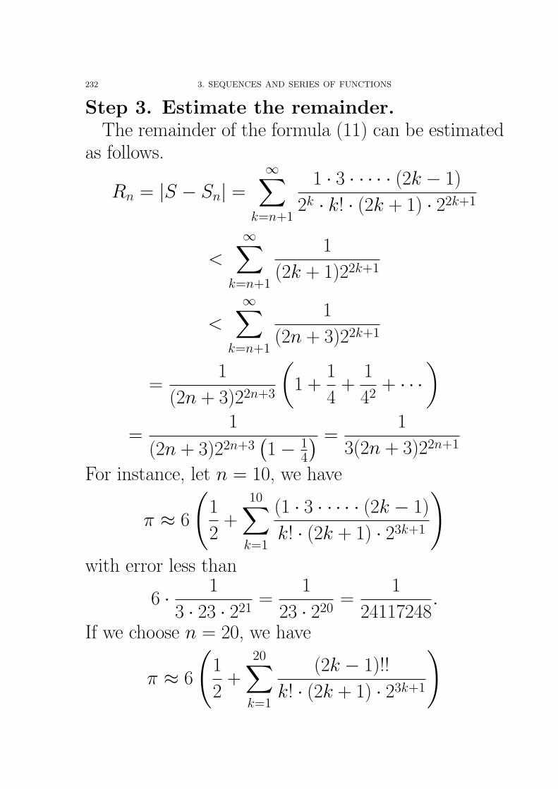
232 3. SEQUENCES AND SERIES OF FUNCTIONS
Step 3. Estimate the remainder.The remainder of the formula (11) can be estimated
as follows.
Rn = |S − Sn| =
∞∑k=n+1
1 · 3 · · · · · (2k − 1)
2k · k! · (2k + 1) · 22k+1
<∞∑
k=n+1
1
(2k + 1)22k+1
<∞∑
k=n+1
1
(2n + 3)22k+1
=1
(2n + 3)22n+3
(1 +
1
4+
1
42+ · · ·
)=
1
(2n + 3)22n+3(1− 1
4
) =1
3(2n + 3)22n+1
For instance, let n = 10, we have
π ≈ 6
(1
2+
10∑k=1
(1 · 3 · · · · · (2k − 1)
k! · (2k + 1) · 23k+1
)with error less than
6 · 1
3 · 23 · 221=
1
23 · 220=
1
24117248.
If we choose n = 20, we have
π ≈ 6
(1
2+
20∑k=1
(2k − 1)!!
k! · (2k + 1) · 23k+1
)
8. TAYLOR SERIES 233
with error less than
6 · 1
3 · 43 · 241=
1
43 · 240=
1
47278999994368< 10−13.
If n = 40, the error is less than1
100340843028014221500612608< 10−26.
234 3. SEQUENCES AND SERIES OF FUNCTIONS
Remark. There are several other methods for computing π. Forinstance, we can also use
π
4= arctan 1 = 1− 1
3+
1
5− 1
7+ · · · ,
but one needs a huge number of terms to get enough accuracy.(So this method is no good for computational purpose!) Anothermethod is to use the formula of John Machin (1680-1751):
4 arctan1
5− arctan
1
239=
π
4,
see our text book [6, Problem 7, p.813] for details. Machin usedhis method in 1706 to find π correct to 100 decimal places. In1995 Jonathan and Peter Borwein of Simon Fraster Universityand Yasumasa Kanada of the University of Tokyo calculated thevalue of π to 4, 294, 967, 286 decimal places!
Another story on computing π is a Chinese mathematicianand astronomer Tsu Ch’ung Chi (430-501). He gave the rational
approximation355
113to π which is correct to 6 decimal places. He
also proved that
3.1415926 < π < 3.1415927
a remarkable result (Note. He was a person lived 1500 yearsago!), on which it would be nice to have more details but TsuCh’ung Chi’s book, written with his son, is lost. (His methodis to cut off the circle by equal pieces to get his approximationto π.) Tsu’s astronomical achievements include the making of anew calendar in 463 which never came into use. (According tothe article of J J O’Connor and E F Robertson in http://www-groups.dcs.st-and.ac.uk/ history/Mathematicians/Tsu.html.)
Remark. Those, who are interested in more applications ofTaylor series, can try to finish the applied project, Radiationfrom the Stars, in our text book [6, pp.808-809].
Bibliography
[1] R. G. Bartle and D. R. Sherbert, Introduction to real analysis, 3rd edition, John Wiley, 2000.(Compulsory reading)
[2] Watson Fulks, Advanced Calculus, 3rd Edition, John Wiley & Sons, Inc. press, 1961.[3] Wilfred Kaplan, Advanced Calculus, 3rd Edition, Addison-Wesley Publishing Company press,
1984.[4] William R. Parzynski and Philip W. Zipse, Introduction to mathematical analysis, Interna-
tional Edition, McGraw-Hill Book Company press,1987.[5] W. Rudin, Principles of Mathematical Analysis, 3rd edition, McGraw-Hill, 1976.[6] James Stewart, Calculus, 4th Edition, Brooks/Cole Publishing Company press, 1999.[7] Manfred Stoll, Real Analysis, 2nd Edition, Addison Wesley Longman, Inc. press, 2001.[8] G. B. Thomas, Jr. and Ross L. Finney, Calculus and analytic geometry, 9th Edition, Interna-
tional Student Edition, Addison-Wesley Longman Inc. press, 1996.
235