lecture notes on advanced calculus ii - dept of maths, nusmatwujie/fall02/lectnotes2.pdf · lecture...
TRANSCRIPT

Lecture Notes On Advanced Calculus II
Jie Wu
Department of Mathematics
National University of Singapore

Contents
Chapter 1. Sequences of Real Numbers 51. Sequences 52. Limits of Sequences 63. Sequences which tend to ∞ 134. Techniques For Computing Limits 155. The Least Upper Bounds and the Completeness Property of R 236. Monotone Sequences 327. Subsequences 358. The Limit Superior and Inferior of a Sequence 389. Cauchy Sequences and the Completeness of R 60
Chapter 2. Series of Real Numbers 651. Series 652. Tests for Positive Series 743. The Dirichlet Test and Alternating Series 964. Absolute and Conditional Convergence 1055. Remarks on the various tests for convergence/divergence of series 108
Chapter 3. Sequences and Series of Functions 1111. Pointwise Convergence 1112. Uniform Convergence 1213. Uniform Convergence of {Fn} and Continuity 1384. Uniform Convergence and Integration 1445. Uniform Convergence and Differentiation 1556. Power Series 1687. Differentiation of Power Series 1888. Taylor Series 197
Bibliography 219
3

CHAPTER 1
Sequences of Real Numbers
1. Sequences
A sequence is an ordered list of numbers. For example,
1, 2, 3, 4, 5, 6
The order of the sequence is important. For example,
2, 1, 4, 3, 6, 5
is different from above sequence. An infinite sequence is a listwhich does not end. For example,
1, 1/2, 1/3, 1/4, 1/5, · · ·We are going to study infinite sequences. We denote by {an}the sequence
a1, a2, a3, · · · , an, · · ·
Example 1.1. Here are some examples of infinite se-quences.
(1). 1,1
2,1
3, · · · ,
1
n, · · ·
(2).1
3,
1
32,
1
33,
1
34, · · ·
(3). 1,−2, 3,−4, 5, · · ·
Can you find a formula for each of the above sequences?Answer: (1). an = 1/n. (2). an = 1/3n. (3). (−1)n−1n.
5
6 1. SEQUENCES OF REAL NUMBERS
2. Limits of Sequences
Definition 2.1. The limit of {an} is A, and is written as
limn→∞
an = A,
if for any ε > 0, there is a natural number N such that forevery n > N , we have
|an − A| < ε.
Remark. 1. Some sequences do not satisfy the above. Wecall such sequences divergent.
2. Sequences which satisfy the above definition, i.e. A existsand is finite, are called convergent sequences.
Example 2.2. Prove the following limits by using ε−Ndefinition
1) limn→∞
1
n= 0.
2) limn→∞
√n2
n2 + 1= 1.
3) limn→∞
(3
4
)n
= 0.
2. LIMITS OF SEQUENCES 7
Solution. (1). limn→∞
1
n= 0.
Given any ε > 0, we want to find N such that∣∣∣∣1n − 0
∣∣∣∣ < ε
for n > N , i.e.,
n >1
εfor n > N . Choose N to be the smallest integer such that
N ≥ 1
ε.
(N is found now!) When n > N , then
n > N ≥ 1
εor ∣∣∣∣1n − 0
∣∣∣∣ < ε.
Thus limn→∞
1
n= 0.
8 1. SEQUENCES OF REAL NUMBERS
(2). limn→∞
√n2
n2 + 1= 1.
Given any ε > 0, we want to find N such that∣∣∣∣∣√
n2
n2 + 1− 1
∣∣∣∣∣ < ε
for n > N . Now∣∣∣∣∣√
n2
n2 + 1− 1
∣∣∣∣∣ < ε ⇐⇒∣∣∣∣ n√
n2 + 1− 1
∣∣∣∣ < ε
⇐⇒
∣∣∣∣∣n−√
n2 + 1√n2 + 1
∣∣∣∣∣ < ε ⇐⇒∣∣∣∣ n2 − (n2 + 1)√
n2 + 1(n +√
n2 + 1)
∣∣∣∣ < ε
⇐⇒ 1√n2 + 1(n +
√n2 + 1)
< ε
⇐⇒√
n2 + 1(n +√
n2 + 1) >1
εObserve that √
n2 + 1(n +√
n2 + 1) > n
for n ≥ 1. Choose N to be the smallest integer such that
N ≥ 1
ε.
Then, for n > N ,√
n2 + 1(n +√
n2 + 1) >√
N 2 + 1(N +√
N 2 + 1)
> N ≥ 1
εor ∣∣∣∣∣
√n2
n2 + 1− 1
∣∣∣∣∣ < ε.
Thus N is found and hence the result.
2. LIMITS OF SEQUENCES 9
(3). limn→∞
(3
4
)n
= 0.
Given any ε > 0, we want to find N such that∣∣∣∣(3
4
)n
− 0
∣∣∣∣ < ε
for n > N . Observe that (3
4
)n
< ε
⇐⇒ n ln
(3
4
)< ln(ε)
⇐⇒ n >ln(ε)
ln(3/4)
(Note. ln(3/4) < 0!!) Choose N to be the smallest positiveinteger such that
N ≥ ln(ε)
ln(3/4).
When n > N , then
n > N ≥ ln(ε)
ln(3/4)or∣∣∣∣(3
4
)n
− 0
∣∣∣∣ < ε.
The proof is finished. �
10 1. SEQUENCES OF REAL NUMBERS
Theorem 2.3. If {an} has a limit, then the limit is unique.
Proof. Let A and B be limits of {an}. Suppose that A 6=
B. Choose ε =|A−B|
2.
Then ε > 0 because A 6= B. By definition, there exists N1
and N2 such that|an − A| < ε
for n > N1 and|an −B| < ε
for n > N2.For n > max{N1, N2}, we have
|A−B| = |(A− an) + (an −B)| ≤ |A− an| + |an −B|
< 2ε = 2|A−B|
2= |A−B|,
which is a contradiction. Thus A = B. �
2. LIMITS OF SEQUENCES 11
Theorem 2.4 (Squeeze or Sandwich Theorem). Given threesequences
{an}, {bn}, {cn}such that
(i) an ≤ bn ≤ cn for every n and
(ii) limn→∞
an = A = limn→∞
cn,
then limn→∞
bn = A.
Remark. The above theorem is still applicable if the inequal-ity
an ≤ bn ≤ cn
is true eventually.
Proof. For any ε > 0, there exists N1 and N2 such that
|cn − A| < ε
for n > N1 and|an − A| < ε
for n > N2. Let N = max{N1, N2}. For n > N , we have
−ε < cn − A < ε and − ε < an − A < ε
A− ε < cn < A + ε and A− ε < an < A + ε.
Thus
A− ε < an ≤ bn ≤ cn < A + ε or |bn − A| < ε.
By definition, we have limn→∞
bn = A and hence the result. �
12 1. SEQUENCES OF REAL NUMBERS
Example 2.5. Find limits
1) limn→∞
1 + sin n
n.
2)
(3n− 1
4n + 1
)n
.
Solution. (1). Since
0 ≤ 1 + sin n
n≤ 2
n
and limn→∞
2
n= lim
n→∞0 = 0, we have
limn→∞
1 + sin n
n= 0.
(2). Since
0 ≤(
3n− 1
4n + 1
)n
≤(
3
4
)n
and limn→∞
(3
4
)n
= limn→∞
0 = 0, we have
limn→∞
(3n− 1
4n + 1
)n
= 0.
�
3. SEQUENCES WHICH TEND TO ∞ 13
3. Sequences which tend to ∞Definition 3.1. {an} tends to +∞ if for each number
k, there is an N such that
an > k for all n > N.
Remark. For such sequences, we write as an → +∞ asn →∞ or
limn→∞
an = +∞.
{an} tends to −∞ if for each number k, there is an N suchthat
an < k for all n > N.
In this case, write limn→∞
an = −∞.
Example 3.2. The following sequences tend to +∞1) an =
√ln n.
2) an = (3/2)n.
The sequences − ln n, −n2 and etc then tend to −∞.

14 1. SEQUENCES OF REAL NUMBERS
Theorem 3.3 (Reciprocal Rule). Consider a sequence {an}.
(i) If an > 0 for all n and limn→∞
1
an= 0, then
limn→∞
an = +∞.
(ii) If limn→∞
an = ±∞, then limn→∞
1
an= 0.
Proof. We only prove (i). For each positive integer k, thereexists N such that ∣∣∣∣ 1
an− 0
∣∣∣∣ < 1
k
for n > N because limn→∞
1
an= 0. Then, for n > N , an > k
because an > 0. This finishes the proof. �
Example 3.4. Since limn→∞
1√n
= 0, we have limn→∞
√n = ∞.
Similarly, since limn→∞
√n = +∞, we have lim
n→∞
1√n
= 0.
4. TECHNIQUES FOR COMPUTING LIMITS 15
4. Techniques For Computing Limits
Theorem 4.1. Let f be a continuous function. Then
limn→∞
f (an) = f ( limn→∞
an).
Idea of Proof. By the definition of continuity, when x →x0, f (x) → f (x0). Now lim
n→∞an = A means that an → A when
n →∞. Thus f (an) → f (A) when n →∞, that is,
limn→∞
f (an) = f (A) = f ( limn→∞
an).
�
Example 4.2.
limn→∞
sin
(nπ
2n + 1
)= lim
n→∞
(π
2 + 1/n
)= sin
(π
2
)= 1.
16 1. SEQUENCES OF REAL NUMBERS
Theorem 4.3 (L’Hopital’s Rule). Suppose an = f (n),
bn = g(n) for differentiable functions f and g. If limn→∞
f (n)
g(n)
is of the form∞∞
or0
0, then
limn→∞
f (n)
g(n)= lim
n→∞
f ′(n)
g′(n).
History Remark. Although the theorem is named afterMarquis de l’Hospital (1661-1704), it should be called Bernoulli’srule. The story is that in 1691, l’Hopital asked Johann Bernoulli(1667-1748) to provide, for a fee, lectures on the new subjectof calculus. L’Hopital subsequently incorporated these lecturesinto the first calculus text, L’Analyse des infiniment petis(Analysis of infinitely small quantities), published in 1696.The initial version of what is now known as l’Hopital’s rule firstappeared in this text.
Example 4.4. Show that limn→∞
(1 +
x
n
)n
= ex.
Proof.
limn→∞
ln[(
1 +x
n
)n]= lim
n→∞n ln
(1 +
x
n
)= lim
n→∞
ln(1 + x
n
)1/n
= limn→∞
11+x
n·(− x
n2
)− 1
n2
= limn→∞
x
1 + xn
= x.
Thus limn→∞
(1 +
x
n
)n
= ex. �
4. TECHNIQUES FOR COMPUTING LIMITS 17
Theorem 4.5. If limn→∞
an and limn→∞
bn exist, then
(1). limn→∞
(an + bn) = limn→∞
an + limn→∞
bn,
(2). limn→∞
kan = k limn→∞
an,
(3). limn→∞
anbn = limn→∞
an limn→∞
bn,
(4). limn→∞
an
bn=
limn→∞
an
limn→∞
bn, provided bn 6= 0 and lim
n→∞bn 6= 0.
Proof. omitted. �
Example 4.6. Find the limit of
ln
(n2 + 3n + 2
2 + 4n + 2n2
)+ cos
(1√n
).
Solution.
limn→∞
[ln
(n2 + 3n + 2
2 + 4n + 2n2
)+ cos
(1√n
)]= lim
n→∞
[ln
((n2 + 3n + 2)/n2
(2 + 4n + 2n2)/n2
)+ cos
(1√n
)]= lim
n→∞
[ln
(1 + 3/n + 2/n2
2/n2 + 4/n + 2
)+ cos
(1√n
)]= ln
(1 + 0 + 0
0 + 0 + 2
)+ cos 0 = ln
(1
2
)+ 1 = 1− ln 2.
�
18 1. SEQUENCES OF REAL NUMBERS
Theorem 4.7 (Some Standard Limits). Some standardlimits are given as follows.
1. limn→∞
1
np= 0 for any fixed p > 0.
2. limn→∞
cn = 0 for any fixed c where |c| < 1.
3. limn→∞
c1n = 1 for any fixed c > 0.
4. limn→∞
n√
n = 1.
5. limn→∞
np
cn= 0 for any fixed p and c > 1.
6. limn→∞
cn
n!= 0 for any fixed c.
7. limn→∞
(1 +
x
n
)n
= ex for any fixed x.
8. limn→∞
(ln n)p
nk= 0 for any fixed k > 0.

4. TECHNIQUES FOR COMPUTING LIMITS 19
Proof. 1. limn→∞
1
np= 0 for any fixed p > 0.
limn→∞
1
np=(
limn→∞
1
n
)p
= 0p = 0.
2. limn→∞
cn = 0 for any fixed c where |c| < 1.
Case 1: When c = 0, the statement is obvious.
Case 2: When c > 0, we have
ln(
limn→∞
cn)
= limn→∞
ln cn = limn→∞
n ln c = −∞.
Thus, limn→∞
cn = 0.
Case 3: When c < 0, we have −|c|n ≤ cn ≤ |c|n for all n.By Case 2, we have lim
n→∞(−|c|n) = 0 = lim
n→∞|c|n. Hence by
Squeeze theorem, we also have limn→∞
cn = 0.
3. limn→∞
c1n = 1 for any fixed c > 0.
limn→∞
c1n = climn→∞ 1
n = c0 = 1.

20 1. SEQUENCES OF REAL NUMBERS
4. limn→∞
n√
n = 1.
ln(
limn→∞
n√
n)
= limn→∞
ln n√
n
= limn→∞
ln n
n= 0 (by L’Hopital’s rule).
Thus, limn→∞
n√
n = e0 = 1.
5. limn→∞
np
cn= 0 for any fixed p and c > 1.
Let k be a fixed positive integer such that p− k < 0. Then
limn→∞
np
cn= lim
n→∞
pnp−1
cn ln c= lim
p(p− 1)np−2
cn(ln c)2= · · ·
= limn→∞
p(p− 1) · · · (p− k + 1)np−k
cn(ln c)k
= limn→∞
p(p− 1) · · · (p− k + 1)
cnnk−p(ln c)k= 0
by L’Hopital’s rule.
4. TECHNIQUES FOR COMPUTING LIMITS 21
6. limn→∞
cn
n!= 0 for any fixed c.
Let an =cn
n!=
c · c · · · · · cn(n− 1) · · · · · 1
. Now fix an integer M > c.
Then for any n > M ,
0 < an =c · c · · · · · c
n(n− 1) · · · · · (M + 1)aM <
c
naM .
Note that aM is a fixed number because M is fixed. Since
limn→∞
0 = 0 = limn→∞
c
naM , by the Squeeze theorem, lim
n→∞an = 0.
7. limn→∞
(1 +
x
n
)n
= ex for any fixed x. It was proved in
Example 4.4.
8. limn→∞
(ln n)p
nk= 0 for any fixed k > 0.
Let m = ln n. Then n = em. By (5),
limn→∞
(ln n)p
nk= lim
m→∞
mp
ekm= lim
m→∞
mp
(ek)m = 0,
where ek > 1 because k > 0. �
22 1. SEQUENCES OF REAL NUMBERS
Strategy: One can find the limits of many sequences fromthose of the standard sequences.
Example 4.8. Find the limits
1) limn→∞
8n + (ln n)10 + n!
n6 − n!.
2) limn→∞
(1− 1
2n + 1
)3n
.
Solution. (1).
limn→∞
8n + (ln n)10 + n!
n6 − n!= lim
n→∞
8n/n! + (ln n)10/n! + 1
n6/n!− 1
=0 + 0 + 1
0− 1= −1.
(2).
limn→∞
(1− 1
2n + 1
)3n
= limn→∞
[(1 +
−1
2n + 1
)2n+1] 3n
2n+1
= limn→∞
[(1 +
−1
2n + 1
)2n+1] 3
2+1/n
=(e−1)3
2 =1
e√
e
�
5. THE LEAST UPPER BOUNDS AND THE COMPLETENESS PROPERTY OF R 23
5. The Least Upper Bounds and theCompleteness Property of R
5.1. From Natural Numbers to Real Numbers.Starting with natural numbers N = {1, 2, 3, · · · }, we obtainreal numbers R by adding more and more new numbers in thefollowing steps:
Step 1. By adding 0 and negative numbers, we have integersZ = {0,±1,±2,±3, · · · }.
Step 2. Then we have rational numbers Q =
{p
q
∣∣∣ p, q ∈ Z, q 6= 0
}.
Step 3. Then, by adding irrational numbers, we have allreal numbers.
Below we give some examples of irrational numbers. Re-call that a natural number p > 1 is called prime if p is NOTdivisible by any natural numbers other than p and 1. For in-stance, 2, 3, 5, 7, 11, · · · are primes. Every natural numbern > 1 admits a unique (prime) factorization
n = p1 · p2 · · · pk,
where each pi is prime. For instance, 20 = 2 · 2 · 5 and 66 =2 · 3 · 11.
24 1. SEQUENCES OF REAL NUMBERS
Example 5.1. If n is a natural number, and there is nonatural number whose square is n, then
√n is NOT a ra-
tional number. In particular,√
2,√
3,√
5,√
6 are irrationalnumbers.
Proof. Suppose that√
n is a rational number. We can
write√
n asa
b, where a, b ∈ N and b 6= 0. Then
√n =
a
b⇐⇒ n =
a2
b2⇐⇒ a2 = b2n.
Any prime occurring in the (unique) factorization of a will occuran even number of times in the factorization of a2; similarly forb and b2.
By a2 = b2n, any prime that occurs in the factorization of nmust occur an even number of times, since all primes occurringin the factorization of b2n are exactly those occurring in thefactorization of a2.
Thus n can be written as
n = (p1 · p2 · · · pk)2,
where, of course, the pi’s need not be distinct.
This, however, is a contradiction to the hypothesis, since nis expressed as the square of a natural number. �
5. THE LEAST UPPER BOUNDS AND THE COMPLETENESS PROPERTY OF R 25
5.2. Bounded Sets.
Definition 5.2. A set of real numbers S is boundedabove if there exists a finite real number M such that
x ≤ M ∀x ∈ S.
M is called an upper bound of S.
Definition 5.3. A set of real numbers S is bounded be-low if there exists a finite real number m such that
m ≤ x ∀x ∈ S.
m is called a lower bound of S.
Definition 5.4. A set which is both bounded above andbelow is called a bounded set.
Remark.1. Upper bounds and lower bounds are not unique.
2. Some sets only have upper bounds but not lower bounds.
3. Some sets have only lower bounds but not upper bounds.
4. A set which is not bounded is called an unbounded set.
Example 5.5. Let S = {r | r is a rational number with r <√2}. Then S is bounded above.
26 1. SEQUENCES OF REAL NUMBERS
Theorem 5.6. Every convergent sequence is bounded.
Proof. Let {an} be a sequence convergent to A. For ε = 1,there exists N such that |an −A| < 1 or A− 1 < an < A + 1for n > N .
Choose M and m to be the largest and smallest number ofthe finite numbers
a1, a2, . . . , aN , A + 1, A− 1,
respectively.
When n ≤ N , we have m ≤ an ≤ M because M (m) is thelargest (smallest) number of the above finite set. When n > N ,we have
m ≤ A− 1 < an < A + 1 ≤ M.
Thus, for all n, we have m ≤ an ≤ M and so {an} is bounded.The proof is finished. �
Corollary 5.7 (Test for divergence). If {an} is unbounded,then {an} diverges.
Remark.1. The converse may not be true, i.e., divergent sequence neednot be unbounded.
2. The inverse may not be true, i.e., a bounded sequence maynot be convergent.
Example. The sequence {1,−1, 1,−1, · · · } is bounded butNOT convergent.

5. THE LEAST UPPER BOUNDS AND THE COMPLETENESS PROPERTY OF R 27
5.3. Infimum and Supremum. Recall that any finiteset of real numbers has a greatest element (maximum) and aleast element (minimum).
Example 5.8. {−2.5, 3.1, −4.4, 4.5, 5}
However, this property does not necessarily hold for infinitesets.
Example 5.9. {1, 2, 3, 4, · · · , }.
Definition 5.10. A real number M ( 6= ±∞) is called theleast upper bound or supremum of a set E if
(i) M is an upper bound of E, i.e., x ≤ M for everyx ∈ E, and
(ii) if M ′ < M , then M ′ is not an upper bound of E (i.e.,there is an x ∈ E such that M ′ < x).
We write M = sup E.
28 1. SEQUENCES OF REAL NUMBERS
Remark.(i) sup E is unique whenever it exists.
(ii) The main difference between sup E and max E is thatsup E need not be an element of E, whereas max E mustbe an element of E if it does exist).
(iii) If E has a maximum, then sup E = max E.
Example 5.11. 1. Let E = {r ∈ Q | 0 ≤ r ≤√
2}. Thensup E =
√2 but max E does not exist because
√2 is not a
rational number, that is, sup E 6∈ E.
2. Let E = {1/2, 2/3, 3/4, 4/5, 5/6, · · · }. Then sup E = 1and max E does not exist.
3. Let E = {1, 1/2, 1/3, 1/4, 1/5, · · · }. Then max E = 1 =sup E.
5. THE LEAST UPPER BOUNDS AND THE COMPLETENESS PROPERTY OF R 29
Definition 5.12. A real number m ( 6= ±∞) is called thegreatest lower bound or infimum of a set E if
(i) m is a lower bound of E, i.e., m ≤ x for every x ∈ E,and
(ii) if m′ > m, then m′ is not a lower bound of E (i.e.,there exists an x ∈ E such that x < m′).
We write m = inf E.
Remark.(i) inf E is unique whenever it exists.
(ii) The main difference between inf E and min E is that inf Eneed not be an element of E, whereas min E must be anelement of E if it does exist.
(iii) If E has a minimum, then inf E = min E.
Example 5.13. 1. Let E = {1, 1/2, 1/3, 1/4, · · · , }. Theninf E = 0 but min E does not exist.
2. Let E = {r ∈ Q | 0 ≤ r ≤√
2}. Then min E = inf E = 0.
30 1. SEQUENCES OF REAL NUMBERS
5.4. The Completeness of R. Consider the set E ={r ∈ Q | r2 < 2}. Then E is a bounded subset of rationalnumbers, but sup E =
√2 is NOT a rational number. For con-
sidering sup and inf of bounded subsets of rational numbers,we may obtain irrational numbers. For bounded subsets ofreal numbers, sup and inf are still real numbers. This is calledcompleteness property of R. In details, we have the fol-lowing.
Theorem 5.14 (Completeness Axiom of R). The followingstatement hold for subsets of real numbers:
(i) If E is bounded above, then sup E exists.
(ii) If E is bounded below, then inf E exists.
Remark. For assertion (i), it just means that if a subset ofreal numbers E is bounded above, then sup E exists as a realnumber. Compare with rational case: if a subset of rationalnumbers E is bounded above, then sup E exists only as a realnumber, but it need not be a rational number.
5. THE LEAST UPPER BOUNDS AND THE COMPLETENESS PROPERTY OF R 31
Remark. Richard Dedekind (a German mathematician, 1831-1916), in 1872, used algebraic techniques to construct real num-ber system R from Q. His basic ideas are as follows.
Given a rational number r, we can construct two sets U ={x ∈ Q | x ≥ r} and L = {x ∈ Q | x < r}. (One can alsoconstruct U = {x ∈ Q | x > r} and L = {x ∈ Q | x ≤ r}.)The sets U and L have the property that
(1). U and L are subsets of Q;(2). U ∪ L = Q;(3). U 6= ∅;(4). L 6= ∅;(5). U ∩ L = ∅; and(6). every element in U is greater than every element in
L.
Such a paring (U,L) is called a Dedekind cut. Thenwe can use inf U (or sup L) to define a new number. This isDedekind’s idea to construct all real numbers by using rationalnumbers. For instance, let U = {x ∈ Q | x2 > 2} and L ={x ∈ Q | x2 > 2}. Then inf U = sup L =
√2. Another way to
construct real numbers using rational numbers was introducedby Georg Cantor (1845-1917). We will explain Cantor’s ideasin the section of Cauchy sequences.
Recall that a set E is bounded if and only if it is boundedabove and bounded below. Thus the Completeness Axiom leadsto
Corollary 5.15. If E is bounded, then both sup Eand inf E exist.
32 1. SEQUENCES OF REAL NUMBERS
6. Monotone Sequences
Definition 6.1. {an} is called monotone increasing(decreasing) if
an ≤ (≥) an+1
for every n, that is,
a1 ≤ a2 ≤ a3 ≤ a4 ≤ · · ·(a1 ≥ a2 ≥ a3 ≥ · · · ).
Example 6.2. (1). The sequence {1/n} is monotone de-creasing.
(2). The sequence {1/2, 2/3, 3/4, 4/5, 5/6, · · · } is monotoneincreasing.
Proposition 6.3. A monotone increasing (decreas-ing) sequence is bounded below (above).
Proof. Let {an} be a monotone increasing sequence, thatis,
a1 ≤ a2 ≤ a3 ≤ · · · .
Then a1 is a lower bound for {an} and hence the result. �
6. MONOTONE SEQUENCES 33
Theorem 6.4 (Monotone Convergence Theorem). Let {an}be a sequence.
(i) If {an} is monotone increasing and bounded above,then {an} is convergent and
limn→∞
an = supn
an.
(ii) If {an} is monotone decreasing and boundedbelow, then {an} is convergent and
limn→∞
an = infn
an.
Proof. (i). Suppose {an} is monotone increasing and boundedabove.
Then by the Completeness Axiom of R, supn
an exists (finite).
Now, given ε > 0, since supn
an − ε < supn
an, it follows that
supn
an − ε is not an upper bound of {an}.In other words, there exists an integer N such that aN >
supn
an − ε. Then for all n > N , we have
supn
an − ε < aN ≤ an ≤ supn
an < supn
an + ε (since n > N).
Equivalently,
∣∣∣∣an − supn
an
∣∣∣∣ < ε for all n > N and so limn→∞
an =
supn
an (exists).
The proof of (ii) is similar. �
34 1. SEQUENCES OF REAL NUMBERS
Example 6.5. Let an =n
n + 1, that is,
{an} = {1/2, 2/3, 3/4, · · · }.Then an is monotone increasing and bounded above. Thus
supn
an = limn→∞
an = 1.
Corollary 6.6. If {an} is monotone increasing (de-creasing), then either
(i) {an} is convergent or(ii) lim
n→∞an = +∞(−∞).
Proof. Suppose {an} is monotone increasing, then either{an} is bounded above or not bounded above.
Case (a): If {an} is bounded above, then by the MonotoneConvergence Theorem, {an} converges.
Case (b): If {an} is not bounded above, then {an} has noupper bounds. Thus for any given k > 0, k is not an upperbound of {an}. In other words, there exists N such that
aN > k.
Since {an} is monotone increasing, it follows that for all n > N ,
an ≥ aN > k.
Therefore, limn→∞
an = +∞.
The proof for the case when {an} is monotone decreasing issimilar. �
7. SUBSEQUENCES 35
7. Subsequences
Example 7.1. The following are the subsequences of {an} ={1,−1, 1,−1, 1,−1, · · · }.{a2n−1} = {1, 1, 1, · · · }{a2n} = {−1,−1,−1, · · · }.
In general, subsequences of {an} are of the form {ank},
k = 1, 2, 3, ..., with
n1 < n2 < n3 < · · · .
Note. The rule is that we should choose an1 first and then an2with n2 > n1 and then an3 with n3 > n2, so far and so on (upto infinite). Thus n1 is at least 1, n2 is at least 2, n3 is at least3, · · · .
36 1. SEQUENCES OF REAL NUMBERS
Theorem 7.2. Suppose limn→∞
an = A. Then every sub-
sequence of {an} also converges to A, that is,
limk→∞
ank= A.
Proof. For any given ε > 0, since limn→∞
an = A, there exists
N such that
|an − A| < ε for all n > N.
Then for all k > N , we have
nk ≥ k > N.
Hence|ank
− A| < ε for all k > N.
Therefore, limk→∞
ank= A. �
7. SUBSEQUENCES 37
Corollary 7.3. Suppose that {an} has two subsequencesthat converge to different limits. Then {an} is di-vergent. �
Example 7.4. The sequence {1,−1, 1,−1, · · · } is diver-gent because {a2n−1} = {1, 1, · · · } converges to 1 and {a2n} ={−1,−1, · · · } converges to −1.
38 1. SEQUENCES OF REAL NUMBERS
8. The Limit Superior and Inferior of a Sequence
Given a sequence {an}, we can form another sequence {bn}given by
bn = supk≥n
ak = sup{an, an+1, an+2, · · · }.
Example 8.1. Let {an} = {1,−1, 1,−1, · · · }. Then
bn = supk≥n
ak = sup{±1,∓1,±1,∓1, · · · } = 1.
Proposition 8.2. For any sequence {an}, the associ-ated sequence {bn} = {sup
k≥nak} is always monotone
decreasing.
Proof. For each n,
bn = sup{an, an+1, an+2, · · · } ≥ sup{an+1, an+2, · · · } = bn+1.
�
Definition 8.3. The limit superior of {an}, denoted bylim sup an or lim sup
n→∞an or lim
n→∞an is defined to be lim
n→∞bn, i.e.
limn→∞
an = limn→∞
bn = limn→∞
supk≥n
ak.
8. THE LIMIT SUPERIOR AND INFERIOR OF A SEQUENCE 39
Example 8.4. 1. Let {an} = {1,−1, 1,−1, 1,−1, · · · }.lim
n→∞an = lim
n→∞bn = lim
n→∞1 = 1.
2. Let {an} = {1, 2, 3, · · · }. Then
bn = supk≥n
ak = sup{n, n + 1, · · · } = +∞
and so limn→∞
an = limn→∞
bn = +∞.
3. Let {an} = {−1,−2,−3, · · · }. Then
bn = supk≥n
ak = sup{−n,−n− 1, · · · } = −n
and so limn→∞
an = limn→∞
bn = −∞.
40 1. SEQUENCES OF REAL NUMBERS
Theorem 8.5. Given any sequence {an}, either
(1). limn→∞
an exists (finite), or
(2). limn→∞
an = +∞, or
(3). limn→∞
an = −∞.
Proof. If {an} is not bounded above, then each bn is +∞,and thus
limn→∞
an = limn→∞
bn = +∞.
If {an} is bounded above, then each bn is finite. Since {bn}is monotone decreasing, by Corollary 1.7.3, {an} converges (toa finite limit), or lim
n→∞bn = −∞. �

8. THE LIMIT SUPERIOR AND INFERIOR OF A SEQUENCE 41
Similarly, given any sequence {an}, we can form anothersequence {cn} given by
cn = infk≥n
ak = inf{an, an+1, an+2, · · · }.
Definition 8.6. The limit inferior of {an}, denoted bylim inf an or lim inf
n→∞an or lim
n→∞an is defined to be lim
n→∞cn, i.e.
limn→∞
an = limn→∞
cn = limn→∞
infk≥n
ak.
42 1. SEQUENCES OF REAL NUMBERS
Example 8.7. 1. Let {an} = {1,−1, 1,−1, 1,−1, · · · }.lim
n→∞an = lim
n→∞cn = lim
n→∞(inf{±1,∓1,±1,∓1, · · · )
= limn→∞
−1 = −1.
2. Let {an} = {1, 2, 3, · · · }. Then
cn = infk≥n
ak = inf{n, n + 1, · · · } = n
and so limn→∞
an = limn→∞
cn = +∞.
3. Let {an} = {−1,−2,−3, · · · }. Then
cn = infk≥n
ak = inf{−n,−n− 1, · · · } = −∞
and so limn→∞
an = limn→∞
cn = −∞.
Proposition 8.8. (i). As in Proposition 8.2, for anygiven sequence {an}, the associated sequence {cn} ={ inf
k≥nak} is always monotone increasing.
(ii). As in Theorem 8.5, for any given {an}, limn→∞
an either
exists (finite), or +∞, or −∞).
Remark. We always have
limn→∞
an ≤ limn→∞
an
because cn ≤ bn.
8. THE LIMIT SUPERIOR AND INFERIOR OF A SEQUENCE 43
Proposition 8.9. (i). If limn→∞
an = B with B 6= −∞,
then given ε > 0, there exists N such that
an < B + ε
for all n > N .
(ii). limn→∞
an = C with C 6= +∞, then given ε > 0, there
exists N such thatan > C − ε
for all n > N .
Proof. (i). If B = +∞, the assertion is obvious and sowe assume that B is finite.
Since limn→∞
an = B, given any ε > 0, there exists N such
that for all n > N ,
|bn−B| < ε =⇒ bn < B+ε =⇒ sup{an, an+1, · · · } < B+ε,
i.e. an, an + 1, · · · < B + ε for all n > N .
Proof of (ii) is similar. �
44 1. SEQUENCES OF REAL NUMBERS
Warning!! Given a sequence {an}, limn→∞
an is a different con-
cept from supn
an. From the definition, we have
b1 = supn
an = sup{a1, a2, · · · }
bn = sup{an, an+1, an+2, · · · }with b1 ≥ b2 ≥ b3 ≥ · · · and lim
n→∞an = lim
n→∞bn. Thus we have
the relationlim
n→∞an ≤ sup
nan = b1,
but limn→∞
an need not be equal to supn
an in general.
Similarly,lim
n→∞an ≥ inf
nan = c1,
but need not be equal to in general.
The correct understanding is that lim is the largest sub-sequential limit of convergent subsequences, including thosepossible subsequences tending to +∞ or −∞. Similarly, lim isthe smallest subsequential limit. This is described in thefollowing theorem.
8. THE LIMIT SUPERIOR AND INFERIOR OF A SEQUENCE 45
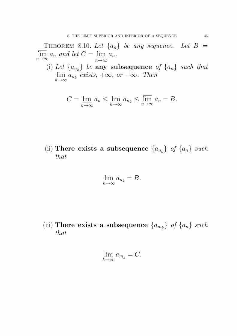
Theorem 8.10. Let {an} be any sequence. Let B =lim
n→∞an and let C = lim
n→∞an.
(i) Let {ank} be any subsequence of {an} such that
limk→∞
ankexists, +∞, or −∞. Then
C = limn→∞
an ≤ limk→∞
ank≤ lim
n→∞an = B.
(ii) There exists a subsequence {ank} of {an} such
that
limk→∞
ank= B.
(iii) There exists a subsequence {amk} of {an} such
that
limk→∞
amk= C.
46 1. SEQUENCES OF REAL NUMBERS
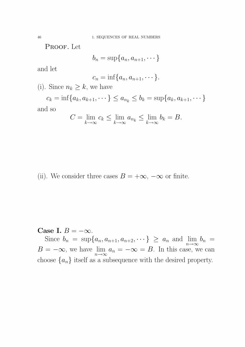
Proof. Let
bn = sup{an, an+1, · · · }and let
cn = inf{an, an+1, · · · }.(i). Since nk ≥ k, we have
ck = inf{ak, ak+1, · · · } ≤ ank≤ bk = sup{ak, ak+1, · · · }
and soC = lim
k→∞ck ≤ lim
k→∞ank
≤ limk→∞
bk = B.
(ii). We consider three cases B = +∞, −∞ or finite.
Case I. B = −∞.Since bn = sup{an, an+1, an+2, · · · } ≥ an and lim
n→∞bn =
B = −∞, we have limn→∞
an = −∞ = B. In this case, we can
choose {an} itself as a subsequence with the desired property.
8. THE LIMIT SUPERIOR AND INFERIOR OF A SEQUENCE 47
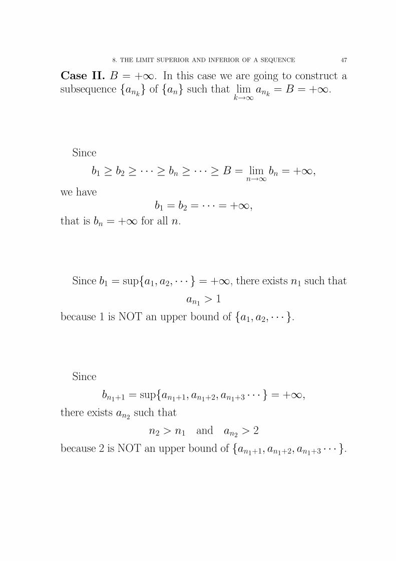
Case II. B = +∞. In this case we are going to construct asubsequence {ank
} of {an} such that limk→∞
ank= B = +∞.
Since
b1 ≥ b2 ≥ · · · ≥ bn ≥ · · · ≥ B = limn→∞
bn = +∞,
we haveb1 = b2 = · · · = +∞,
that is bn = +∞ for all n.
Since b1 = sup{a1, a2, · · · } = +∞, there exists n1 such that
an1 > 1
because 1 is NOT an upper bound of {a1, a2, · · · }.
Since
bn1+1 = sup{an1+1, an1+2, an1+3 · · · } = +∞,
there exists an2 such that
n2 > n1 and an2 > 2
because 2 is NOT an upper bound of {an1+1, an1+2, an1+3 · · · }.
48 1. SEQUENCES OF REAL NUMBERS
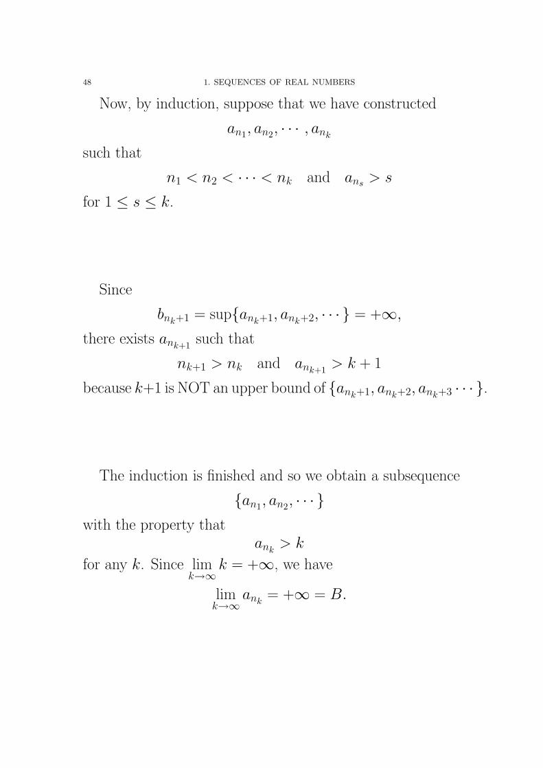
Now, by induction, suppose that we have constructed
an1, an2, · · · , ank
such that
n1 < n2 < · · · < nk and ans > s
for 1 ≤ s ≤ k.
Since
bnk+1 = sup{ank+1, ank+2, · · · } = +∞,
there exists ank+1 such that
nk+1 > nk and ank+1 > k + 1
because k+1 is NOT an upper bound of {ank+1, ank+2, ank+3 · · · }.
The induction is finished and so we obtain a subsequence
{an1, an2, · · · }with the property that
ank> k
for any k. Since limk→∞
k = +∞, we have
limk→∞
ank= +∞ = B.
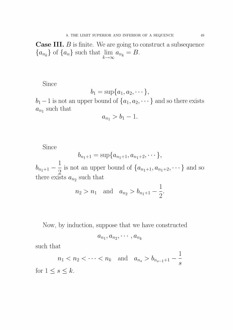
8. THE LIMIT SUPERIOR AND INFERIOR OF A SEQUENCE 49
Case III. B is finite. We are going to construct a subsequence{ank
} of {an} such that limk→∞
ank= B.
Sinceb1 = sup{a1, a2, · · · },
b1−1 is not an upper bound of {a1, a2, · · · } and so there existsan1 such that
an1 > b1 − 1.
Sincebn1+1 = sup{an1+1, an1+2, · · · },
bn1+1 −1
2is not an upper bound of {an1+1, an1+2, · · · } and so
there exists an2 such that
n2 > n1 and an2 > bn1+1 −1
2.
Now, by induction, suppose that we have constructed
an1, an2, · · · , ank
such that
n1 < n2 < · · · < nk and ans > bns−1+1 −1
sfor 1 ≤ s ≤ k.
50 1. SEQUENCES OF REAL NUMBERS
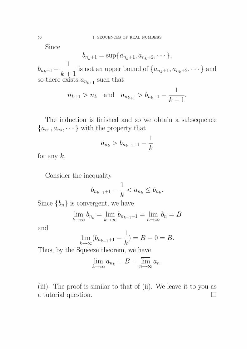
Sincebnk+1 = sup{ank+1, ank+2, · · · },
bnk+1−1
k + 1is not an upper bound of {ank+1, ank+2, · · · } and
so there exists ank+1 such that
nk+1 > nk and ank+1 > bnk+1 −1
k + 1.
The induction is finished and so we obtain a subsequence{an1, an2, · · · } with the property that
ank> bnk−1+1 −
1
kfor any k.
Consider the inequality
bnk−1+1 −1
k< ank
≤ bnk.
Since {bn} is convergent, we have
limk→∞
bnk= lim
k→∞bnk−1+1 = lim
n→∞bn = B
and
limk→∞
(bnk−1+1 −1
k) = B − 0 = B.
Thus, by the Squeeze theorem, we have
limk→∞
ank= B = lim
n→∞an.
(iii). The proof is similar to that of (ii). We leave it to you asa tutorial question. �
8. THE LIMIT SUPERIOR AND INFERIOR OF A SEQUENCE 51
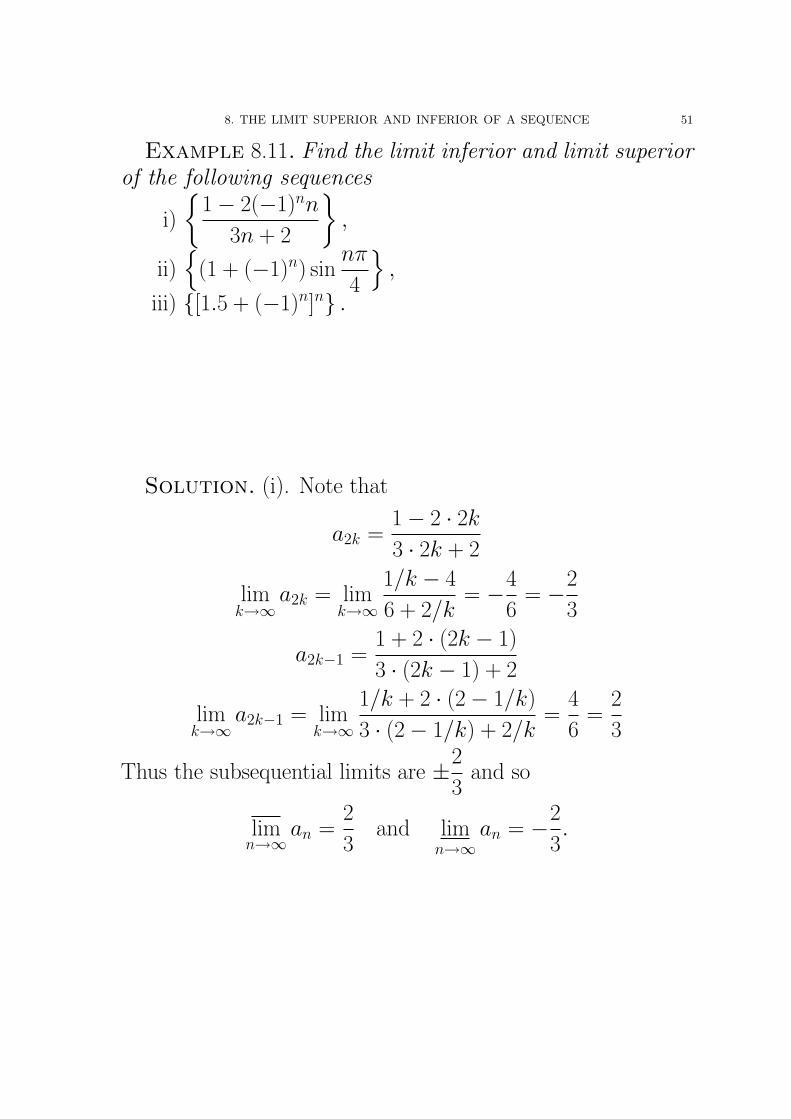
Example 8.11. Find the limit inferior and limit superiorof the following sequences
i)
{1− 2(−1)nn
3n + 2
},
ii){
(1 + (−1)n) sinnπ
4
},
iii) {[1.5 + (−1)n]n} .
Solution. (i). Note that
a2k =1− 2 · 2k3 · 2k + 2
limk→∞
a2k = limk→∞
1/k − 4
6 + 2/k= −4
6= −2
3
a2k−1 =1 + 2 · (2k − 1)
3 · (2k − 1) + 2
limk→∞
a2k−1 = limk→∞
1/k + 2 · (2− 1/k)
3 · (2− 1/k) + 2/k=
4
6=
2
3
Thus the subsequential limits are ±2
3and so
limn→∞
an =2
3and lim
n→∞an = −2
3.
52 1. SEQUENCES OF REAL NUMBERS
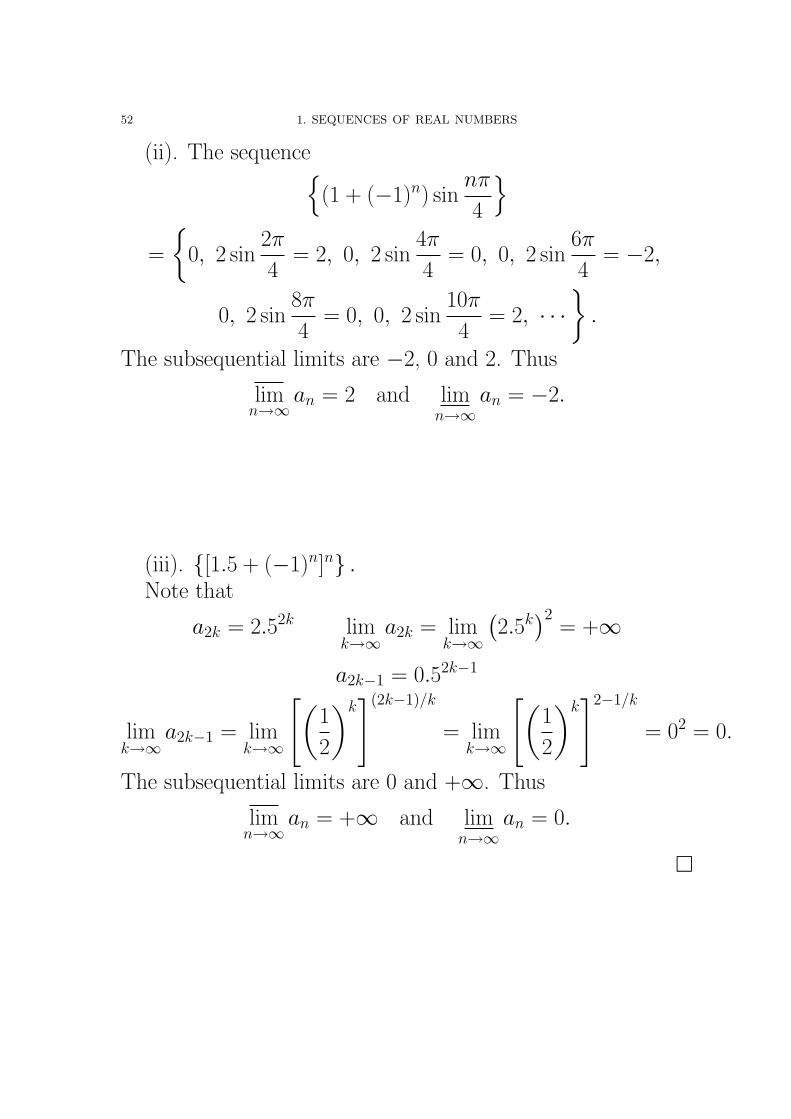
(ii). The sequence{(1 + (−1)n) sin
nπ
4
}=
{0, 2 sin
2π
4= 2, 0, 2 sin
4π
4= 0, 0, 2 sin
6π
4= −2,
0, 2 sin8π
4= 0, 0, 2 sin
10π
4= 2, · · ·
}.
The subsequential limits are −2, 0 and 2. Thus
limn→∞
an = 2 and limn→∞
an = −2.
(iii). {[1.5 + (−1)n]n} .Note that
a2k = 2.52k limk→∞
a2k = limk→∞
(2.5k
)2= +∞
a2k−1 = 0.52k−1
limk→∞
a2k−1 = limk→∞
[(1
2
)k](2k−1)/k
= limk→∞
[(1
2
)k]2−1/k
= 02 = 0.
The subsequential limits are 0 and +∞. Thus
limn→∞
an = +∞ and limn→∞
an = 0.
�
8. THE LIMIT SUPERIOR AND INFERIOR OF A SEQUENCE 53
The following theorem was originally proved by BernhardBolzano (1781-1848) and modified slightly by Karl Weierstrass(1815-1897).
Corollary 8.12 (Bolzano-Weierstrass). Every boundedsequence has a convergent subsequence.
Proof. Let {an} be a bounded sequence. Since {an} isbounded,
−∞ < inf{a1, a2, · · · } = c1 ≤ limn→∞
an
≤ limn→∞
an ≤ b1 = sup{a1, a2, · · · } < +∞.
Thus limn→∞
an is finite.
By Part (ii) of Theorem 8.10, there exists a convergent sub-sequence {ank
} of {an} such that
limk→∞
ank= lim
n→∞an.
�
54 1. SEQUENCES OF REAL NUMBERS
Theorem 8.13. limn→∞
an = limn→∞
an (finite, +∞, −∞) if
and only if limn→∞
an exists (finite), +∞, or −∞.
Proof. Suppose that limn→∞
an = limn→∞
an = A. Let bn =
sup{an, an+1, · · · } and let cn = inf{an, an+1, · · · }.
Then
cn = inf{an, an+1, · · · } ≤ an ≤ bn = sup{an, an+1, · · · }.
By the assumption, we have
limn→∞
cn = limn→∞
an = limn→∞
an = limn→∞
bn.
By the Squeeze theorem, the sequence {an} converges and
limn→∞
an = limn→∞
an = limn→∞
an.
Conversely suppose that {an} converges, tends to +∞, ortends to −∞. Let A = lim
n→∞an and let {ank
} be any subse-
quence of {an}.
By Theorem 7.2, we have limk→∞
ank= A. Thus the only
subsequential limit of {an} is A.
By Theorem 8.10, we have
limn→∞
an = limn→∞
an = A = limn→∞
an.
�
8. THE LIMIT SUPERIOR AND INFERIOR OF A SEQUENCE 55
Remark. This theorem means that
1) If limn→∞
an = limn→∞
an, then
limn→∞
an = limn→∞
an = limn→∞
an.
2) If limn→∞
an exists, +∞ or −∞, then
limn→∞
an = limn→∞
an = limn→∞
an.
Example 8.14. Let {an} be a sequence. Show that
limn→∞
|an| = 0
if and only iflim
n→∞|an| = 0,
if and only iflim
n→∞an = 0.
56 1. SEQUENCES OF REAL NUMBERS
Proof. Suppose that limn→∞
|an| = 0. From |an| ≥ 0, we
have
0 = limn→∞
0 = limn→∞
0 ≤ limn→∞
|an| ≤ limn→∞
|an| = 0.
Thuslim
n→∞|an| = lim
n→∞|an| = 0
and so limn→∞
|an| exists and
limn→∞
|an| = limn→∞
|an| = limn→∞
|an| = 0
Conversely suppose that limn→∞
|an| = 0. Then
limn→∞
|an| = limn→∞
|an| = limn→∞
|an| = 0
because {an} is convergent. Hence limn→∞
|an| = 0 if and only if
limn→∞
|an| = 0.
Now suppose that limn→∞
|an| = 0. From
−|an| ≤ an ≤ |an|,we have lim
n→∞an = 0 by the Squeeze theorem.
Conversely suppose that limn→∞
an = 0. Then
limn→∞
|an| = | limn→∞
an| = |0| = 0
because the function f (x) = |x| is continuous. Hence
limn→∞
|an| = 0 ⇐⇒ limn→∞
an = 0.
�
8. THE LIMIT SUPERIOR AND INFERIOR OF A SEQUENCE 57
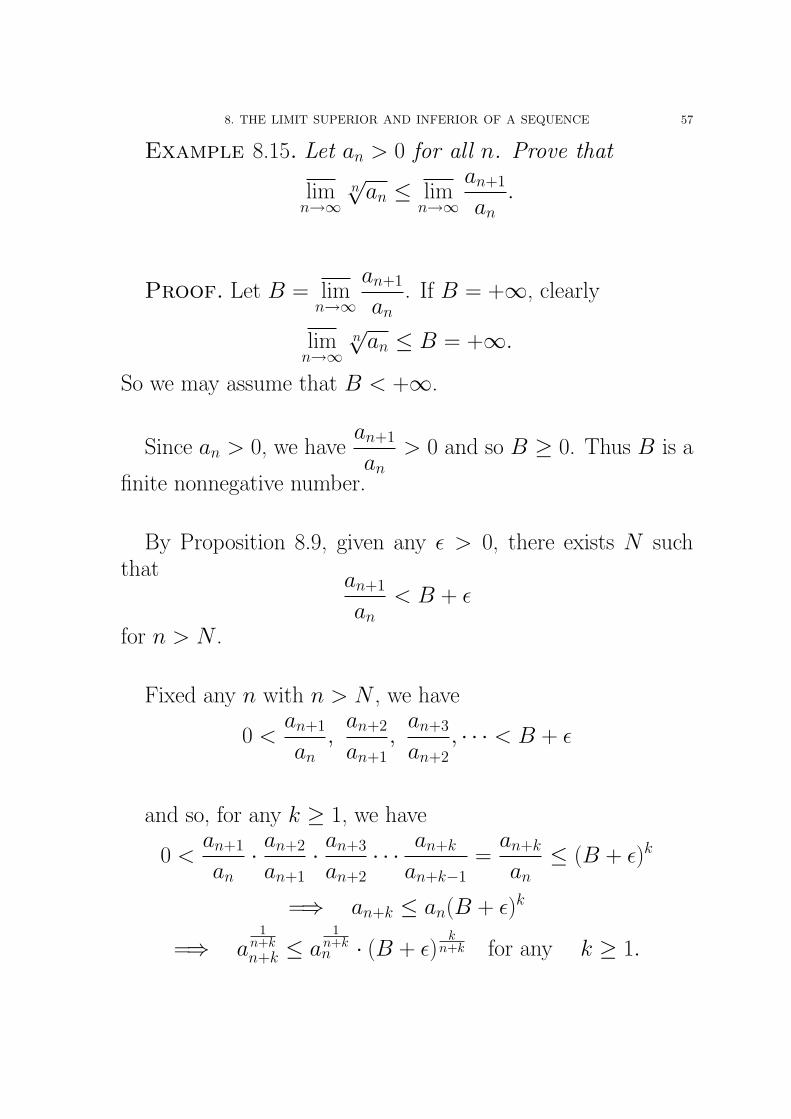
Example 8.15. Let an > 0 for all n. Prove that
limn→∞
n√
an ≤ limn→∞
an+1
an.
Proof. Let B = limn→∞
an+1
an. If B = +∞, clearly
limn→∞
n√
an ≤ B = +∞.
So we may assume that B < +∞.
Since an > 0, we havean+1
an> 0 and so B ≥ 0. Thus B is a
finite nonnegative number.
By Proposition 8.9, given any ε > 0, there exists N suchthat an+1
an< B + ε
for n > N .
Fixed any n with n > N , we have
0 <an+1
an,
an+2
an+1,
an+3
an+2, · · · < B + ε
and so, for any k ≥ 1, we have
0 <an+1
an· an+2
an+1· an+3
an+2· · · an+k
an+k−1=
an+k
an≤ (B + ε)k
=⇒ an+k ≤ an(B + ε)k
=⇒ a1
n+kn+k ≤ a
1n+kn · (B + ε)
kn+k for any k ≥ 1.

58 1. SEQUENCES OF REAL NUMBERS
Let k tends to ∞. We have
limk→∞
a1
n+kn · (B + ε)
kn+k
= limk→∞
a1
n+kn · lim
k→∞(B + ε)
1n/k+1 = a0
n · (B + ε) = B + ε.
Thus
limm→∞
a1mm = lim
k→∞a
1n+kn+k ≤ lim
k→∞a
1n+kn · (B + ε)
kn+k
= limk→∞
a1
n+kn · (B + ε)
kn+k = B + ε.
In other words,
limn→∞
n√
an ≤ B + ε
for any ε > 0
and so
limn→∞
n√
an = limε→0
(lim
n→∞n√
an
)≤ lim
ε→0(B + ε) = B,
that is,
limn→∞
n√
an ≤ limn→∞
an+1
an.
�
8. THE LIMIT SUPERIOR AND INFERIOR OF A SEQUENCE 59
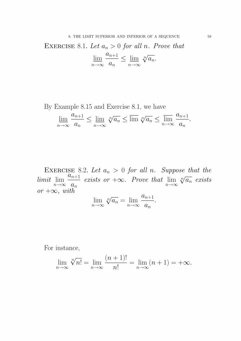
Exercise 8.1. Let an > 0 for all n. Prove that
limn→∞
an+1
an≤ lim
n→∞n√
an.
By Example 8.15 and Exercise 8.1, we have
limn→∞
an+1
an≤ lim
n→∞n√
an ≤ lim n√
an ≤ limn→∞
an+1
an.
Exercise 8.2. Let an > 0 for all n. Suppose that the
limit limn→∞
an+1
anexists or +∞. Prove that lim
n→∞n√
an exists
or +∞, with
limn→∞
n√
an = limn→∞
an+1
an.
For instance,
limn→∞
n√
n! = limn→∞
(n + 1)!
n!= lim
n→∞(n + 1) = +∞.
60 1. SEQUENCES OF REAL NUMBERS
9. Cauchy Sequences and the Completeness of R9.1. Cauchy Sequences.
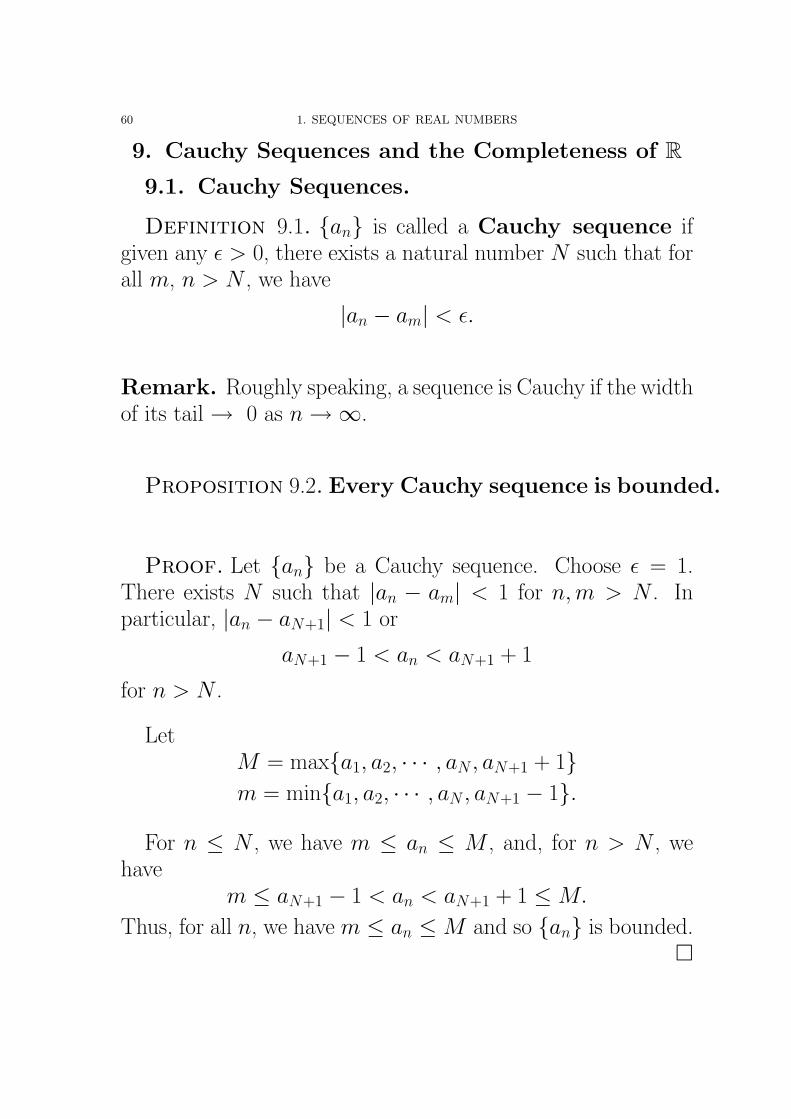
Definition 9.1. {an} is called a Cauchy sequence ifgiven any ε > 0, there exists a natural number N such that forall m, n > N , we have
|an − am| < ε.
Remark. Roughly speaking, a sequence is Cauchy if the widthof its tail → 0 as n →∞.
Proposition 9.2. Every Cauchy sequence is bounded.
Proof. Let {an} be a Cauchy sequence. Choose ε = 1.There exists N such that |an − am| < 1 for n,m > N . Inparticular, |an − aN+1| < 1 or
aN+1 − 1 < an < aN+1 + 1
for n > N .
LetM = max{a1, a2, · · · , aN , aN+1 + 1}m = min{a1, a2, · · · , aN , aN+1 − 1}.
For n ≤ N , we have m ≤ an ≤ M , and, for n > N , wehave
m ≤ aN+1 − 1 < an < aN+1 + 1 ≤ M.
Thus, for all n, we have m ≤ an ≤ M and so {an} is bounded.�

9. CAUCHY SEQUENCES AND THE COMPLETENESS OF R 61
9.2. Completeness of R. The following Criterion wasformulated by Augustin-Louis Cauchy (1789-1857).
Theorem 9.3 (Cauchy’s criterion). A sequence is aconvergent sequence if and only if it is a Cauchysequence.
Proof. =⇒, i.e., every convergent sequence is Cauchy.
Given that {an} is convergent, say limn→∞
an = A. Then for
any given ε > 0, there exists N such that
|an − A| < ε
2for all n > N. Now for any m,n > N ,
|an−am| = |(an−A)−(am−A)| ≤ |an−A|+|am−A| < ε
2+
ε
2= ε
since both m,n > N . Therefore, {an} is a Cauchy sequence.
62 1. SEQUENCES OF REAL NUMBERS
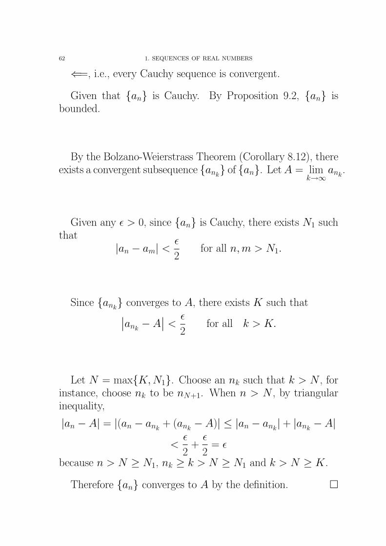
⇐=, i.e., every Cauchy sequence is convergent.
Given that {an} is Cauchy. By Proposition 9.2, {an} isbounded.
By the Bolzano-Weierstrass Theorem (Corollary 8.12), thereexists a convergent subsequence {ank
} of {an}. Let A = limk→∞
ank.
Given any ε > 0, since {an} is Cauchy, there exists N1 suchthat
|an − am| <ε
2for all n,m > N1.
Since {ank} converges to A, there exists K such that∣∣ank
− A∣∣ < ε
2for all k > K.
Let N = max{K, N1}. Choose an nk such that k > N , forinstance, choose nk to be nN+1. When n > N , by triangularinequality,
|an − A| = |(an − ank+ (ank
− A)| ≤ |an − ank| + |ank
− A|
<ε
2+
ε
2= ε
because n > N ≥ N1, nk ≥ k > N ≥ N1 and k > N ≥ K.
Therefore {an} converges to A by the definition. �
9. CAUCHY SEQUENCES AND THE COMPLETENESS OF R 63
Remark. The statement that every Cauchy sequence inR converges is often expressed by saying that R is complete.Note that our proof of the Cauchy Criterion used the Bolzano-Weierstrass Theorem and the proof of that one used the com-pleteness axiom of R (Theorem 5.14). We did not prove Theo-rem 5.14, namely we treated Theorem 5.14 as an axiom. (Dedekindand Cantor proved the completeness axiom in 1872 indepen-dently.) Conversely, we can treat the Cauchy Criterion as anaxiom, and prove Theorem 5.14. In this sense, both Theorem5.14 and the Cauchy Criterion are regarded as the completenessof R.
Cantor constructed real numbers from rational numbers byusing Cauchy sequences. His ideas are as follows. Consider allof the Cauchy sequences {an} with an ∈ Q. By the Cauchycriterion, {an} converges to a real number. Then he provedthat all real numbers can be obtained as the limits of all of theCauchy sequences {an} with an ∈ Q. One can think that, byusing our standard base 10 number system, any real numberadmits a (decimal) expansion. For instance,
√2 = 1.4142 · · · ,
we can define a sequence of rational numbers
a1 = 1, a2 = 1.4, a3 = 1.41, a4 = 1.414, a5 = 1.4142, · · · with limn→∞
an =√
2.
64 1. SEQUENCES OF REAL NUMBERS
Example 9.4. Let sn = 1 +1
22+
1
32+ · · ·+ 1
n2. Show that
{sn} is convergent.
Proof. For each k ≥ 1, we have
|sn+k−sn| =
∣∣∣∣(1 +1
22+ · · · + 1
n2+
1
(n + 1)2+ · · · + 1
(n + k)2
)−(
1 +1
22+ · · · + 1
n2
)∣∣∣∣=
1
(n + 1)2+
1
(n + 2)2+ · · · + 1
(n + k)2
≤ 1
n(n + 1)+
1
(n + 1)(n + 2)+
1
(n + 2)(n + 3)
+ · · · + 1
(n + k − 1)(n + k)
=
(1
n− 1
n + 1
)+
(1
n + 1− 1
n + 2
)+· · ·+
(1
n + k − 1− 1
n + k
)=
1
n− 1
n + k<
1
n.
Given any ε > 0, choose N such that 1N < ε, that is, N >
1
ε.
When m > n > N , from the above,
|sm − sn| <1
n<
1
N< ε.
Thus {sn} is a Cauchy sequence and hence {sn} converges bythe Cauchy Criterion. �
CHAPTER 2
Series of Real Numbers
1. Series
The expression
a1 + a2 + a3 + · · ·
written alternatively as
∞∑k=1
ak is called an infinite series.
Example 1.1. (1). 1 + 2 + 3 + 4 + · · · .
(2). 1 + 1/2 + 1/3 + 1/4 + · · ·
(3). 1 + 1/22 + 1/32 + 1/42 + · · · .
(4). 1 + 0 + 1 + 0 + 1 + 0 + · · · .
Definition 1.2. Given a series
∞∑k=1
ak, its nth partial sum
Sn is given by
Sn =
n∑k=1
ak = a1 + a2 + · · · + an.
The sequence {Sn} is called the sequence of partial sums
of the series
∞∑k=1
ak.
Example 1.3. Consider the series 1− 1 + 1− 1 + 1− 1 +1− 1 + · · · . The S2n−1 = 1 and S2n = 0.
65
66 2. SERIES OF REAL NUMBERS
Definition 1.4. Consider the sequence of partial sums {Sn}
of the series
∞∑k=1
ak. If this sequence converges to a number S,
we say that the series
∞∑k=1
ak converges to S and write
∞∑k=1
ak = limn→∞
Sn = S.
If {Sn} diverges, then we say
∞∑k=1
an diverges.

1. SERIES 67
Example 1.5 (Geometric Series). Let a 6= 0. Consider theseries ∞∑
n=0
arn = a + ar + ar2 + ar3 + · · · .
Then the partial sum
Sn = a + ar + ar2 + · · · + arn−1 = a(1 + r + · · · + rn−1)
=
a1− rn
1− rr 6= 1
a(n + 1) r = 1
When −1 < r < 1, Sn →a
1− ras n →∞.
When r > 1, Sn diverges because rn → +∞ as n →∞.
When r = 1, Sn = a(n + 1) diverges.
When r = −1, Sn =a[1− (−1)n]
2diverges.
When r < −1, Sn diverges because rn → ±∞.
Thus the geometric series∞∑
n=0
arn converges if and
only if −1 < r < 1, and,∞∑
n=0
arn =a
1− r
for −1 < r < 1.
68 2. SERIES OF REAL NUMBERS
Remark. If
∞∑k=1
ak and
∞∑k=1
bk converges, then one always has
(i)
∞∑k=1
(ak + bk) =
∞∑k=1
ak +
∞∑k=1
bk.
(ii)
∞∑k=1
cak = c
∞∑k=1
ak.
Example 1.6.∞∑
n=1
[(1
4
)n
+
(1
5
)n]=
∞∑n=1
(1
4
)n
+
∞∑n=1
(1
5
)n
=
[1
4+
(1
4
)2
+ · · ·
]+
[1
5+
(1
5
)2
+ · · ·
]
=1
4
[1 +
1
4+
(1
4
)2
+ · · ·
]+
1
5
[1 +
1
5+
(1
5
)2
+ · · ·
]=
1
4
1
1− 1
4
+1
5
1
1− 1
5
=1
4 · 3
4
+1
5 · 4
5
=1
3+
1
4=
7
12.
1. SERIES 69
Theorem 1.7. If∞∑
k=1
ak converges, then limk→∞
ak = 0.
Proof. Recall that partial sum Sk = a1 + a2 + · · · + ak.We have
Sk − Sk−1 = (a1 + a2 + · · · + ak−1 + ak)
− (a1 + a2 + · · · + ak−1) = ak.
Since the series
∞∑k=1
ak converges, the sequence {Sk} con-
verges. Let S = limk→∞
Sk. Then
limk→∞
ak = limk→∞
(Sk−Sk−1) = limk→∞
Sk− limk→∞
Sk−1 = S−S = 0.
�
Corollary 1.8 (Divergence Test). If limn→∞
an 6= 0 (or
does not exist), then∞∑
n=1
an diverges. �
70 2. SERIES OF REAL NUMBERS
Example 1.9. (1). The series
∞∑n=1
(−1)n is divergent be-
cause the limit of the n-th term (−1)n does not exist.
(2). The series
∞∑n=1
n!
n2is divergent because
limn→∞
n!
n2=
1
limn→∞
n2
n!
=1
0= +∞ 6= 0.
(3). The series
∞∑n=1
2n + 1
3n + 2is divergent because
limn→∞
2n + 1
3n + 2= lim
n→∞
2 + 1/n
3 + 2/n=
2
36= 0.
Remark. The divergence test is a “one-way” test, i.e., limn→∞
an =
0 does NOT imply
∞∑n=1
an converges.
1. SERIES 71
Theorem 1.10 (Cauchy Criterion). The series∞∑
k=1
ak con-
verges if and only if given any ε > 0, there exists N suchthat ∣∣∣∣∣
m∑k=n+1
ak
∣∣∣∣∣ < ε
for all m > n > N .
Proof. The series
∞∑k=1
ak converges if and only if the se-
quence of its partial sums {Sn} converges, (by definition), ifand only if {Sn} is Cauchy. The result follows from
|Sm − Sn| = |(a1 + a2 + · · · + an + an+1 + · · · + am)
−(a1 + a2 + · · · + an)|
= |an + an+1 + · · · + am| =
∣∣∣∣∣m∑
k=n+1
ak
∣∣∣∣∣ .�
72 2. SERIES OF REAL NUMBERS
Example 1.11 (Harmonic Series). Show that the series∞∑
n=1
1
ndiverges.
Proof. Note that
|S2n − Sn| =
∣∣∣∣(1 +1
2+ · · · + 1
n+
1
n + 1+ · · · + 1
2n
)−(
1 +1
2+ · · · + 1
n
)∣∣∣∣=
1
n + 1+
1
n + 2+ · · · + 1
2n
≥ 1
2n+
1
2n+ · · · + 1
2n= n · 1
2n=
1
2.
Suppose that the series
∞∑n=1
1
nconverges. Then {Sn} is
Cauchy.
Given ε = 12. There exists N such that |Sm − Sn| <
1
2for all m > n > N . This contradicts to the above fact that
|S2n − Sn| ≥1
2, where m is chosen to be 2n. �
Note. The divergence of the harmonic series appears to havebeen established by Nicole Oresme (1323?-1382) by showing
that the sequence
{n∑
k=1
1
k
}is NOT bounded.
1. SERIES 73
Theorem 1.12. Suppose that eventually ak ≥ 0. Then∞∑
k=1
ak converges if and only if {Sn} is bounded above.
Proof. We may assume that ak ≥ 0 for all k. Since
Sn+1 − Sn = an+1 ≥ 0,
the sequence {Sn} is monotone increasing.
Thus
∞∑k=1
ak converges if and only if {Sn} converges, if and
only if {Sn} is bounded above (by the Monotone ConvergenceTheorem). �
Note. Suppose that eventually ak ≥ 0. This theorem meansthat the following.
1) If {Sn} is bounded above, then
∞∑k=1
ak converges.
2) If {Sn} is NOT bounded above, then
∞∑k=1
ak diverges.
74 2. SERIES OF REAL NUMBERS
2. Tests for Positive Series
A series
∞∑k=1
ak is called a (eventually) positive series if
every term ak is (eventually) positive.
2.1. Comparison Test.
Theorem 2.1 (Comparison Test). Consider two series∞∑
k=1
ak and∞∑
k=1
bk. Suppose that eventually 0 ≤ ak ≤ bk.
(i) If∞∑
k=1
bk converges, then∞∑
k=1
ak converges.
(ii) If∞∑
k=1
ak diverges, then∞∑
k=1
bk diverges.

2. TESTS FOR POSITIVE SERIES 75
Proof. Assertion (ii) follows immediately from (i).
We may assume that 0 ≤ ak ≤ bk for all k. Let An =
n∑k=1
ak,
and Bn =
n∑k=1
bk. Then An ≤ Bn for all n.
Suppose that
∞∑k=1
bk converges, that is,
∞∑k=1
bk is a (finite)
number. Then
An ≤ Bn ≤∞∑
k=1
bk
for all n and so An is bounded above.
By Theorem 1.12,
∞∑k=1
ak is convergent. �
76 2. SERIES OF REAL NUMBERS
Example 2.2. The series
∞∑k=1
(2k − 1
3k + 2
)k
converges because
(2k − 1
3k + 2
)k
≤(
2
3
)k
and the geometric series
∞∑k=1
(2
3
)k
converges.
Remark. 1. Suppose 0 ≤ an ≤ bn and
∞∑n=1
bn diverges. Then
NO conclusion can be drawn.
2. Similarly, suppose 0 ≤ an ≤ bn and
∞∑n=1
an converges. Then
NO conclusion can be drawn.
Example 2.3.
0 ≤(
1
2
)n
≤ 2n ≤ 3n.
The series
∞∑n=1
3n diverges. Now
∞∑n=1
(1
2
)n
converges and
∞∑n=1
2n diverges.
2. TESTS FOR POSITIVE SERIES 77
Corollary 2.4 (Limit Comparison Test). Suppose that∞∑
k=1
ak and∞∑
k=1
bk are (eventually) positive series.
(a). If limk→∞
ak
bk= L with 0 < L < ∞, then
∞∑k=1
ak con-
verges if and only if∞∑
k=1
bk converges. (So∞∑
k=1
ak
diverges if and only if∞∑
k=1
bk diverges.)
(b). If limk→∞
ak
bk= 0, (that is, ak << bk), and
∞∑k=1
bk con-
verges, then∞∑
k=1
ak converges.
(c). If limk→∞
ak
bk= 0, (that is, ak << bk), and
∞∑k=1
ak di-
verges, then∞∑
k=1
bk diverges.
Remark. If limn→∞
an
bn= +∞, interchange an and bn, and then
apply assertions (b) and (c).

78 2. SERIES OF REAL NUMBERS
Proof. We may assume that
∞∑k=1
ak and
∞∑k=1
bk are positive
series.(a). Since
limk→∞
ak
bk= L ( 6= 0, 6= ∞),{
ak
bk
}is bounded above, say, by M . Thus
0 ≤ ak ≤ Mbk
for all k. Similarly, since limk→∞
bk
ak=
1
L( 6= 0, 6= ∞),
{bk
ak
}is
bounded above, say, by M ′. Thus
0 ≤ bk ≤ M ′ak
for all k.
If
∞∑k=1
ak is convergent, then
∞∑k=1
M ′ak = M ′∞∑
k=1
ak is also
convergent. By the comparison test, it follows that
∞∑k=1
bk is
also convergent because bk ≤ M ′ak.
If
∞∑k=1
bk is convergent, then
∞∑k=1
Mbk = M∞∑
k=1
bk is also
convergent. By the comparison test, it follows that
∞∑k=1
ak is
also convergent because ak ≤ Mbk.
2. TESTS FOR POSITIVE SERIES 79
Hence
∞∑k=1
ak is convergent if and only if
∞∑k=1
bk is convergent.
Hence
∞∑k=1
ak is divergent if and only if
∞∑k=1
bk is divergent.
Now we prove assertions (b) and (c).
limk→∞
ak
bk= 0
implies for every ε > 0, there is an N such that∣∣∣∣ak
bk− 0
∣∣∣∣ < ε ∀k > N.
We choose ε = 1. Then the above inequality is
ak < bk ∀k > N.
We get the result by applying the comparison test. �
80 2. SERIES OF REAL NUMBERS
Standard series used in comparison and limit com-parison tests.1. The Geometric Series:
∞∑n=1
arn−1 =
converges if |r| < 1,
diverges if |r| ≥ 1.
2. The p-series: for a fixed p,
∞∑n=1
1
np=
converges if p > 1,
diverges if p ≤ 1.
To be proved in the subsection on Integral Test.
2. TESTS FOR POSITIVE SERIES 81
Example 2.5. Determine the convergence or divergence:
1)
∞∑n=1
1 + cos n
n2
2)
∞∑n=1
ln n + n3 + 8
n4 − 2n + 3
Solution. (1). It is convergent, by the comparison test,because
0 ≤ 1 + cos n
n2≤ 2
n2
and the p-series
∞∑n=1
1
n2is convergent.
(2). It is divergent, by the limit comparison test, because
limn→∞
ln n + n3 + 8
n4 − 2n + 31
n
= limn→∞
n ln n + n4 + 8n
n4 − 2n + 3
= limn→∞
ln n
n3+ 1 +
1
n3
1− 2
n3+
3
n4
=0 + 1 + 0
1− 0 + 0= 1
and the harmonic series
∞∑n=1
1
ndiverges. �
82 2. SERIES OF REAL NUMBERS
Example 2.6. Determine convergence or divergence of∞∑
n=2
1
(ln n)k, where k is a constant.
Solution. Let bn =1
(ln n)kand let an =
1
n. Then
limn→∞
an
bn= lim
n→∞
1
n1
(ln n)k
= limn→∞
(ln n)k
n= 0.
Since the harmonic series
∞∑n=2
1
nis divergent, the series
∞∑n=2
1
(ln n)k
is divergent for any k. �
2. TESTS FOR POSITIVE SERIES 83
2.2. Integral Test. Let f (x) be a real-valued function on[a, +∞) such that f (x) is Riemann integrable, that is, the inte-
gral
∫ b
a
f (x) dx exists for every b > a. The following theorem
is useful.
Theorem 2.7. Let f (x) be a real-valued function on [a, b].
(a). If f (x) is continuous on [a, b], then f (x) is Rie-mann integrable on [a, b].
(b). If f (x) is monotone on [a, b], then f (x) is Rie-mann integrable on [a, b].
The improper integral is defined by∫ ∞
a
f (x) dx = limb→∞
∫ b
a
f (x) dx = area under f (x) over [a,∞).
Here we say that
∫ ∞
a
f (x) dx converges if the limit
limb→∞
∫ b
a
f (x) dx
exists (finite), i.e., the area under f (x) over [a,∞) is finite.
We also say that
∫ ∞
a
f (x) dx diverges if the limit
limb→∞
∫ b
a
f (x) dx
does not exist.
84 2. SERIES OF REAL NUMBERS
Theorem 2.8 (Integral Test). Let f (x) be an (eventu-ally) positive monotone decreasing function on [1, +∞).
Suppose we have a series∞∑
k=1
ak such that ak = f (k), then
the series∞∑
k=1
ak and the integral
∫ ∞
1
f (x)dx either
both converge or both diverge.
2. TESTS FOR POSITIVE SERIES 85
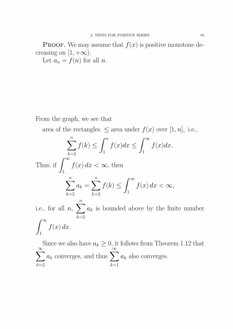
Proof. We may assume that f (x) is positive monotone de-creasing on [1, +∞).
Let an = f (n) for all n.
From the graph, we see that
area of the rectangles ≤ area under f (x) over [1, n], i.e.,n∑
k=2
f (k) ≤∫ n
1
f (x)dx ≤∫ ∞
1
f (x)dx.
Thus, if
∫ ∞
1
f (x) dx < ∞, then
n∑k=2
ak =
n∑k=2
f (k) ≤∫ ∞
1
f (x) dx < ∞,
i.e., for all n,
n∑k=2
ak is bounded above by the finite number∫ ∞
1
f (x) dx.
Since we also have ak ≥ 0, it follows from Theorem 1.12 that∞∑
k=2
ak converges, and thus
∞∑k=1
ak also converges.
86 2. SERIES OF REAL NUMBERS
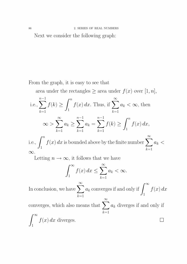
Next we consider the following graph:
From the graph, it is easy to see that
area under the rectangles ≥ area under f (x) over [1, n],
i.e.,
n−1∑k=1
f (k) ≥∫ n
1
f (x) dx. Thus, if
∞∑k=1
ak < ∞, then
∞ >
∞∑k=1
ak ≥n−1∑k=1
ak =
n−1∑k=1
f (k) ≥∫ n
1
f (x) dx,
i.e.,
∫ n
1
f (x) dx is bounded above by the finite number
∞∑k=1
ak <
∞.Letting n →∞, it follows that we have∫ ∞
1
f (x) dx ≤∞∑
k=1
ak < ∞.
In conclusion, we have
∞∑k=1
ak converges if and only if
∫ ∞
1
f (x) dx
converges, which also means that
∞∑k=1
ak diverges if and only if∫ ∞
1
f (x) dx diverges. �
2. TESTS FOR POSITIVE SERIES 87
Example 2.9. Show that
1) the series∞∑
n=1
1
npconverges if and only if p > 1.
2) the series∞∑
n=2
1
n(ln n)kconverges if and only if k > 1.
Proof. (1). If p ≤ 0, then1
npdoes not tend to 0 and so,
by divergence test,
∞∑n=1
1
npdiverges.
Assume that p > 0. Let f (x) =1
xpon [1, +∞). Then f (x)
is positive monotone decreasing. Now
∫ ∞
1
f (x)dx =
∫ ∞
1
x−p dx =
1
−p + 1x−p+1
∣∣∣∣+∞1
p 6= 1
ln(+∞)− ln 1 p = 1
Thus
∫ ∞
1
f (x) dx converges if and only if p > 1 and so
∞∑n=1
1
np
converges if and only if p > 1.
88 2. SERIES OF REAL NUMBERS
(2). the series
∞∑n=2
1
n(ln n)kconverges if and only if k > 1.
Let f (x) =1
x(ln x)kon [2, +∞). Then f (x) is positive. We
check that f (x) is eventually monotone decreasing. From
f ′(x) =(x−1(ln x)−k
)′= −x−2(ln x)−k − kx−1(ln x)−k−1 1
x
= −x−2(ln x)−k−1(ln x + k),
we have f ′(x) ≤ 0 when ln x > −k. Thus f (x) is monotonedecreasing when ln x > −k and so f (x) is eventually monotonedecreasing.
Now∫ ∞
2
f (x) dx =
∫ ∞
2
1
x(ln x)kdx=========
y = ln x
dy =1
xdx
∫ ∞
ln 2
1
ykdy
=
1
−k + 1y−k
∣∣∣∣∞ln 2
k 6= 1
ln(+∞)− ln(ln 2) = +∞ k = 1
Thus
∫ ∞
2
f (x) dx converges if and only if k > 1 and so the
series
∞∑n=2
1
n(ln n)kconverges if and only if k > 1. �
2. TESTS FOR POSITIVE SERIES 89
2.3. Ratio Test.
Theorem 2.10 (Ratio Test). Consider the positive series∞∑
n=1
an. Suppose
(1) limn→∞
an+1
an= `.
(i) If 0 ≤ ` < 1, then∞∑
n=1
an converges.
(ii) If 1 < ` ≤ ∞, then∞∑
n=1
an diverges.
(iii) If ` = 1, then the test is inconclusive.
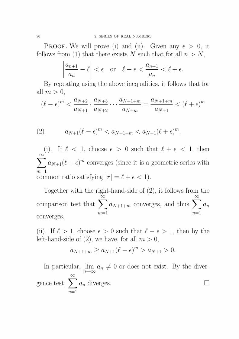
90 2. SERIES OF REAL NUMBERS
Proof. We will prove (i) and (ii). Given any ε > 0, itfollows from (1) that there exists N such that for all n > N ,∣∣∣∣an+1
an− `
∣∣∣∣ < ε or `− ε <an+1
an< ` + ε.
By repeating using the above inequalities, it follows that forall m > 0,
(`− ε)m <aN+2
aN+1· aN+3
aN+2· · · aN+1+m
aN+m=
aN+1+m
aN+1< (` + ε)m
(2) aN+1(`− ε)m < aN+1+m < aN+1(` + ε)m.
(i). If ` < 1, choose ε > 0 such that ` + ε < 1, then∞∑
m=1
aN+1(` + ε)m converges (since it is a geometric series with
common ratio satisfying |r| = ` + ε < 1).
Together with the right-hand-side of (2), it follows from the
comparison test that
∞∑m=1
aN+1+m converges, and thus
∞∑n=1
an
converges.
(ii). If ` > 1, choose ε > 0 such that ` − ε > 1, then by theleft-hand-side of (2), we have, for all m > 0,
aN+1+m ≥ aN+1(`− ε)m > aN+1 > 0.
In particular, limn→∞
an 6= 0 or does not exist. By the diver-
gence test,
∞∑n=1
an diverges. �
2. TESTS FOR POSITIVE SERIES 91
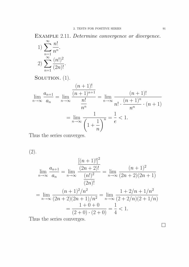
Example 2.11. Determine convergence or divergence.
1)
∞∑n=1
n!
nn.
2)
∞∑n=1
(n!)2
(2n)!.
Solution. (1).
limn→∞
an+1
an= lim
n→∞
(n + 1)!
(n + 1)n+1
n!
nn
= limn→∞
(n + 1)!
n! · (n + 1)n
nn· (n + 1)
= limn→∞
1(1 +
1
n
)n =1
e< 1.
Thus the series converges.
(2).
limn→∞
an+1
an= lim
n→∞
[(n + 1)!]2
(2n + 2)!
(n!)2
(2n)!
= limn→∞
(n + 1)2
(2n + 2)(2n + 1)
= limn→∞
(n + 1)2/n2
(2n + 2)(2n + 1)/n2= lim
n→∞
1 + 2/n + 1/n2
(2 + 2/n)(2 + 1/n)
=1 + 0 + 0
(2 + 0) · (2 + 0)=
1
4< 1.
Thus the series converges.�
92 2. SERIES OF REAL NUMBERS
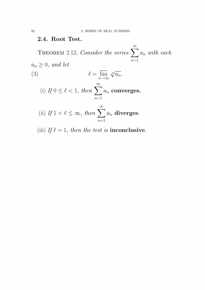
2.4. Root Test.
Theorem 2.12. Consider the series∞∑
n=1
an with each
an ≥ 0, and let
(3) ` = limn→∞
n√
an.
(i) If 0 ≤ ` < 1, then∞∑
n=1
an converges.
(ii) If 1 < ` ≤ ∞, then∞∑
n=1
an diverges.
(iii) If ` = 1, then the test is inconclusive.
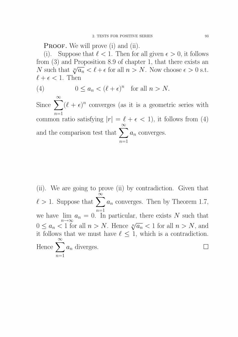
2. TESTS FOR POSITIVE SERIES 93
Proof. We will prove (i) and (ii).(i). Suppose that ` < 1. Then for all given ε > 0, it follows
from (3) and Proposition 8.9 of chapter 1, that there exists anN such that n
√an < `+ ε for all n > N . Now choose ε > 0 s.t.
` + ε < 1. Then
(4) 0 ≤ an < (` + ε)n for all n > N.
Since
∞∑n=1
(` + ε)n converges (as it is a geometric series with
common ratio satisfying |r| = ` + ε < 1), it follows from (4)
and the comparison test that
∞∑n=1
an converges.
(ii). We are going to prove (ii) by contradiction. Given that
` > 1. Suppose that
∞∑n=1
an converges. Then by Theorem 1.7,
we have limn→∞
an = 0. In particular, there exists N such that
0 ≤ an < 1 for all n > N . Hence n√
an < 1 for all n > N , andit follows that we must have ` ≤ 1, which is a contradiction.
Hence
∞∑n=1
an diverges. �

94 2. SERIES OF REAL NUMBERS
Corollary 2.13 (Simplified Root Test). Consider the se-
ries∞∑
n=1
an with each an ≥ 0. Suppose that limn→∞
n√
an = `.
(i) If 0 ≤ ` < 1, then∞∑
n=1
an converges.
(ii) If 1 < ` ≤ ∞, then∞∑
n=1
an diverges.
(iii) If ` = 1, then the test is inconclusive.
Proof. We will prove (i) and (ii). Recall from Theorem 8.13of chapter 1 that if lim
n→∞n√
an exists, then limn→∞
n√
an = limn→∞
n√
an.
Then the Corollary follows from Theorem 2.12. �

2. TESTS FOR POSITIVE SERIES 95
Example 2.14. Determine convergence or divergence ofthe series
∞∑n=1
2n
(1− 1
n
)n2
.
Solution.
limn→∞
n√
an = limn→∞
[2n
(1− 1
n
)n2]1
n= lim
n→∞2
(1− 1
n
)n
=2
e< 1.
Thus the series converges.�
Example 2.15. Determine convergence or divergence ofthe series
∞∑n=1
(3 + sin n)n(
1− 2
n
)n2
.
Proof.
limn→∞
n√
an = limn→∞
[(3 + sin n)n
(1− 2
n
)n2]1
n
= limn→∞
(3 + sin n)
(1− 2
n
)n
≤ limn→∞
4
(1− 2
n
)n
=4
e2< 1.
Thus the series converges. �
96 2. SERIES OF REAL NUMBERS
3. The Dirichlet Test and Alternating Series
3.1. The Dirichlet Test. The following theorem is dueto Neils Abel (1802-1829).
Theorem 3.1 (Abel Partial Summation Formula). Let {ak}and {bk} be sequences, and let {Ak}k≥0 be a sequence suchthat
Ak − Ak−1 = ak
for each k ≥ 1. Then if 1 ≤ p ≤ q,q∑
k=p
akbk = Aqbq − Ap−1bp +
q−1∑k=p
Ak(bk − bk+1).
Proof. Since ak = Ak − Ak−1,
apbp + ap+1bp+1 + · · · + aqbq
= (Ap − Ap−1)bp + (Ap+1 − Ap)bp+1 + (Ap+2 − Ap+1)bp+2
+ · · · + (Aq − Aq−1)bq
= −Ap−1bp + Ap(bp − bp+1) + Ap+1(bp+1 − bp+2)
+ · · · + Aq−1(bq−1 − bq) + Aqbq
= −Ap−1bp + Aqbq +
q−1∑k=p
Ak(bk − bk+1).
�
3. THE DIRICHLET TEST AND ALTERNATING SERIES 97
Remark. There are two canonical choices of {An}
(1). A0 = 0, An =
n∑k=1
ak. Then An − An−1 = an for all n.
(2). Suppose that
∞∑k=1
ak converges. Then we can also choose
{An} by letting An =
n∑k=1
ak −∞∑
k=1
ak = −∞∑
k=n+1
ak,
n ≥ 1, A0 = −∑∞
k=1 ak. In this case, we also have
An − An−1 =
(−
∞∑k=n+1
ak
)−
(−
∞∑k=n
ak
)= an.
98 2. SERIES OF REAL NUMBERS
An application is to give the following theorem of Peter Leje-une Dirichlet (1805-1859).
Theorem 3.2 (Dirichlet Test). Suppose that {ak} and{bk} are sequences of real numbers satisfying the following:
(i). the sequence of the partial sums An =
n∑k=1
ak is
bounded,
(ii). b1 ≥ b2 ≥ b3 ≥ · · · ≥ 0, and
(iii). limk→∞ bk = 0.
Then the series∞∑
k=1
akbk converges.
3. THE DIRICHLET TEST AND ALTERNATING SERIES 99
Proof. Since {An} is bounded, there exists a positive num-ber M > 0 such that |An| < M for all n.
Also, since limn→∞
bn = 0, given ε > 0, there exists N such
that bn = |bn − 0| < ε
2Mfor all n > N .
Now, for m > n > N , by Abel partial summation formula,∣∣∣∣∣m∑
k=n+1
akbk
∣∣∣∣∣ =
∣∣∣∣∣Ambm − Anbn+1 +
m−1∑k=n+1
Ak(bk − bk+1)
∣∣∣∣∣≤ |Am| · |bm| + |An| · |bn+1| +
m−1∑k=n+1
|Ak| · |bk − bk+1|
≤ M · bm + M · bn+1 +
m−1∑k=n+1
M · (bk − bk+1)
(because bk ≥ bk+1 ≥ 0, |Ak| ≤ M)
= M · [bm + bn+1 + (bn+1 − bn+2) + (bn+2 − bn+3) + · · ·+(bm−2 − bm−1) + (bm−1 − bm)]
= 2Mbn+1 < 2M · ε
2M= ε.
Hence by the Cauchy Criterion, the series
∞∑k=1
akbk converges.
�
100 2. SERIES OF REAL NUMBERS
3.2. Alternating Series Test. An alternating seriesis of the form
∞∑n=1
(−1)n+1an = a1 − a2 + a3 − a4 + · · · , or
∞∑n=1
(−1)nan = −a1 + a2 − a3 + a4 − · · ·
with each an > 0.
Example 3.3.
1− 1 + 1− 1 + 1− 1 + 1− 1 + · · ·
1− 1
2+
1
3− 1
4+ · · ·
−1 + 2− 3 + 4− 5 + 6− · · ·
Theorem 3.4 (The Alternating Series test). If {bn} is asequence satisfying
(i) b1 ≥ b2 ≥ b3 ≥ · · · ≥ 0, and
(ii) limn→∞
bn = 0,
then∞∑
n=1
(−1)n+1bn ( and∞∑
n=1
(−1)nbn) converge.
3. THE DIRICHLET TEST AND ALTERNATING SERIES 101
Proof. Let ak = (−1)k+1 and let An =
n∑k=1
ak. Then
|An| =∣∣1− 1 + 1− 1 + · · · + (−1)n + (−1)n+1
∣∣=
{0 when n even1 when n odd
Thus |An| ≤ 1 for all n, and the Dirichlet test applies. �
102 2. SERIES OF REAL NUMBERS
Example 3.5. Show that convergence or divergence ofthe series
∞∑n=1
(−1)n1
np=
convergence p > 0
divergence p ≤ 0.
Proof. If p ≤ 0, then the n-th term (−1)n1
npdoes not tend
to 0. Thus the series diverges in this case by the divergence test.
Assume that p > 0. Let an =1
np. Then an > 0, mono-
tone decreasing and limn→∞
an = 0. Thus the alternating series
converges in this case.
In conclusion, we have that the series
∞∑n=1
(−1)n1
npconverges
when p > 0 and diverges when p ≤ 0. �
3. THE DIRICHLET TEST AND ALTERNATING SERIES 103
Now we are going to give a theorem providing an estimate on
the sum of (certain) series. For instance, let S =
∞∑n=1
(−1)n+1 1
n2.
By taking the partial sum, we have
S ≈ S1 = 1, S ≈ S2 = 1− 1
22= 0.75,
S ≈ S3 = 1− 1
22+
1
32≈ 0.861, . . . .
By using computer program, we are able to compute muchmore, say S1000000. A mathematical problem is then what isthe ‘error’ for estimating S by using the partial sum Sn. Inother words, how to estimate the remainder
Rn = |S − Sn| = |an+1 + an+2 + · · · |.
Theorem 3.6 (Alternating Series Estimation). Let {bn} bea sequence satisfying
(i) b1 ≥ b2 ≥ b3 ≥ · · · ≥ 0, and
(ii) limn→∞
bn = 0.
Let
Sn =
n∑k=1
(−1)k+1bk and S =
∞∑k=1
(−1)k+1bk
Then the remainder Rn = |S − Sn| ≤ bn+1 for all n.
104 2. SERIES OF REAL NUMBERS
Proof.
Rn =∣∣(−1)n+2bn+1 + (−1)n+3bn+2 + · · ·
∣∣= |bn+1 − bn+2 + bn+3 − bn+4 + · · · | .
Sincebn+1 − bn+2 + bn+3 − bn+4 + · · ·
= bn+1−(bn+2−bn+3)−(bn+4−bn+5)−(bn+6−bn+7)−· · · ≤ bn+1
and
bn+1−bn+2+bn+3−bn+4+· · · = (bn+1−bn+2)+(bn+3−bn+4)+· · · ≥ 0,
we have Rn ≤ an+1. �
Example 3.7. Estimate∞∑
n=1
(−1)n+1 1
n4with error within
0.001.
Solution. From1
(n + 1)4≤ 10−3, we have n + 1 ≥ 6 or
n ≥ 5. Thus∞∑
n=1
(−1)n+1 1
n4≈ 1− 1
24+
1
34− 1
44+
1
54
with error within 0.001. �
4. ABSOLUTE AND CONDITIONAL CONVERGENCE 105
4. Absolute and Conditional Convergence
Definition 4.1. A series∞∑
n=1
an is called absolutely
convergent if∞∑
n=1
|an| converges.
Theorem 4.2. Every absolutely convergent seriesis convergent.
Proof. Suppose that
∞∑n=1
an converges absolutely, that is,
∞∑n=1
|an| converges by the definition. Let Tn =
n∑k=1
|ak|, Sn =
n∑k=1
ak.
Since {Tn} converges, {Tn} is Cauchy.
Thus, for any ε > 0, there is a N such that |Tn − Tm| < εfor all n,m > N . For any n,m > N , we may assume thatm ≥ n, say m = n + p (as one of them should be greater thananother). Then
|Sn − Sm| = |Sn − (Sn + an+1 + an+2 + · · · + an+p)|= |an+1 + an+2 + · · · + an+p|
≤ |an+1| + |an+2| + · · · + |an+p| = Tm − Tn = |Tn − Tm| < ε.
Thus {Sn} is a Cauchy sequence and so it converges. Thus
the series
∞∑n=1
an converges and hence the result. �
106 2. SERIES OF REAL NUMBERS
Example 4.3. Determine convergence or divergence ofthe series
∞∑n=2
sin n +1
2n(ln n)2
.
Solution. Since∣∣∣∣∣∣∣sin n +
1
2n(ln n)2
∣∣∣∣∣∣∣ ≤| sin n| + 1
2n(ln n)2
≤1 +
1
2n(ln n)2
and
∞∑n=2
1 +1
2n(ln n)2
=3
2
∞∑n=2
1
n(ln n)2converges by Example 2.9,
the series
∞∑n=2
∣∣∣∣∣∣∣sin n +
1
2n(ln n)2
∣∣∣∣∣∣∣ converges. Thus the series
∞∑n=2
sin n +1
2n(ln n)2
converges. �
Remark. If you are testing for absolute convergence, all thetechniques for the positive series are applicable.
Q: Is the converse of the Corollary true? I.e., if a series isconvergent, will it be absolutely convergent?A: No, it is not necessarily true.
Example 4.4. The series
∞∑n=1
(−1)n1
nconverges by Exam-
ple 3.5, but it is NOT absolutely convergent by the p-series.
4. ABSOLUTE AND CONDITIONAL CONVERGENCE 107
Definition 4.5. A series∞∑
n=1
an is said to be condition-
ally convergent if∞∑
n=1
an converges but∞∑
n=1
|an| diverges.
Example 4.6. The series
∞∑n=1
(−1)n1√n
is conditionally con-
vergent.
Remark 4.7. Every series is either absolutely con-vergent, conditionally convergent or divergent. �
Example 4.8. The series
∞∑n=1
(−1)n1
np=
absolutely convergence p > 1
conditionally convergence 0 < p < 1
divergence p ≤ 0
108 2. SERIES OF REAL NUMBERS
5. Remarks on the various tests forconvergence/divergence of series
1. n-th term test for divergence:- a test for divergence ONLY, and it works for series with
positive and negative terms, e.g.
∞∑n=1
(−1)n.
2. Comparison test/Limit Comparison test:- when applying these tests, one usually compares the given
series with a geometric series or a p-series.- generally works for series which look like the geometric seriesor the p-series,
e.g.
∞∑n=1
2 + (−1)n
4n,
∞∑n=1
21n
n2.
- when an oscillating factor/term appears, e.g.
∞∑n=1
2 + (−1)n
3n,
try the Comparison test rather than the Limit Comparison test.
3. Integral test:
e.g.
∞∑n=2
1
n(ln n)2.
5. REMARKS ON THE VARIOUS TESTS FOR CONVERGENCE/DIVERGENCE OF SERIES109
4. Ratio test:- generally works for series which look like the geometric series,series with n!, and certain series defined recursively,
e.g.
∞∑n=1
n2
3n,
∞∑n=1
(2n)!
4n · n!,
∞∑n=1
an, where a1 = 1, an = (1
2+
1
n)an−1, n = 2, 3, · · · .
5. (Simplified) Root test:- generally works for series where an involves a high power suchas the n-th power,
e.g.
∞∑n=1
n
3n,
∞∑n=1
2n(1− 1
n
)n2
.
6. Alternating Series test: - works for alternating seriesonly,
e.g.
∞∑n=2
(−1)nln n
n.
Remark. In general, Tests 2 - 5 works only for
∞∑n=1
an, where
an ≥ 0.

CHAPTER 3
Sequences and Series of Functions
1. Pointwise Convergence
1.1. Sequences of Functions. Let I be a (nonempty)subset of R, e.g. (−1, 1), [0, 1], etc. For each n ∈ N, let Fn :I → R be a function. Then we say {Fn} forms a sequenceof functions on I .
Example 1.1. (1). Fn(x) = xn, 0 < x < 1. Then{Fn} forms a sequence of functions on (0,1).
(2).{(
1 +x
n
)n}forms a sequence of functions on (−∞,∞).
Write out some terms:
F1(x) = 1 + x F2(x) =(1 +
x
2
)2
F3(x) =(1 +
x
3
)3
If we fix the x, and let n →∞,
limn→∞
Fn(x) = limn→∞
(1 +
x
n
)n
= ex.
So for each x, we can define
F (x) = limn→∞
Fn(x).
111
112 3. SEQUENCES AND SERIES OF FUNCTIONS
Definition 1.2. A sequence {Fn} is said to convergepointwise to a function F on I if
limn→∞
Fn(x) = F (x) for each x ∈ I,
i.e., for each x ∈ I and given any ε > 0, there exists an N(which depends on x and ε) such that
|Fn(x)− F (x)| < ε ∀n > N.
The function F is called the limiting function of {Fn}.
Remark. The limiting function is necessarily unique.
Example 1.3. The sequence {xn} converges pointwise onI = (0, 1) because the limit F (x) = lim
n→∞xn = 0 exists for any
0 < x < 1.
The sequence {xn} does NOT converge on [−1, 1] becausethe limit lim
n→∞xn does not exist when x = −1 ∈ [−1, 1].
1. POINTWISE CONVERGENCE 113
1.2. Series of Functions. A series of functions on aset I is of the form
∞∑n=1
fn(x) = f1(x) + f2(x) + · · · ,
where each fn is a function on I .
Example 1.4. Below are some examples.
1.
∞∑n=1
xn−1 = 1 + x + x2 + x3 + · · ·
2.
∞∑k=1
sin kx
k + x=
sin x
1 + x+
sin 2x
2 + x+
sin 3x
3 + x+· · · , 0 ≤ x ≤ 1.
As in chapter 2, we may form the partial sums
Sn(x) =
n∑k=1
fk(x) = f1(x) + f2(x) + · · · + fn(x).
Then {Sn} forms a sequence of functions on I .
Definition 1.5. The series
∞∑n=1
fn is said to converge
pointwise (to a function S) on I if {Sn} converges pointwise(to S) on I , (i.e. lim
n→∞Sn(x) = S(x) for each x ∈ I .)
114 3. SEQUENCES AND SERIES OF FUNCTIONS
Example 1.6. What is the pointwise limit of∞∑
n=1
xn−1,
where x ∈ (−1, 1)? Does∞∑
n=1
xn−1 converge pointwise on
[−1, 1)
Solution. Consider the partial sum
Sn(x) =
n∑i=1
xi−1 = 1 + x + · · · + xn−1 =1− xn
1− x
for −1 < x < 1. Thus∞∑
n=1
xn−1 = limn→∞
Sn(x) = limn→∞
1− xn
1− x=
1
1− x
for x ∈ (−1, 1).
Since the series
∞∑n=1
xn−1 diverges when x = −1, the series
of functions
∞∑n=1
xn−1 does NOT converge pointwise on [−1, 1).
�
1. POINTWISE CONVERGENCE 115
1.3. Some Questions on Pointwise Convergence.Suppose a sequence of functions {Fn} converges pointwise toa function F on the interval [a, b]. Also suppose a series of
functions
∞∑n=1
fn(x) converges pointwise to a function S(x) on
[a, b]. Among the questions we want to consider the following.Some of these questions were incorrectly believed to be true bymany mathematicians prior to nineteenth century, including thefamous Cauchy. Cauchy in his text Cours d’Analyse “proved”a theorem to the effect that the limit of a convergent sequenceof continuous functions was again continuous. As we will see,this result is false!
Question (a). If each Fn is continuous at p ∈ [a, b], is Fnecessarily continuous at p? Recall that F is continuous at p ifand only if
limt→p
F (t) = F (p).
Since F (x) = limn→∞ Fn(x) for every x ∈ [a, b], what we reallyasking is does
limt→p
(lim
n→∞Fn(t)
)= lim
n→∞
(limt→p
Fn(t)
)?
Question (a’). For series of functions, we can ask similar
question. If each fn(x) is continuous at p, is S(x) =
∞∑n=1
fn(x)
necessarily continuous at p? Again what we really asking isdoes
limt→p
∞∑n=1
fn(t) =
∞∑n=1
limt→p
fn(t) ?
116 3. SEQUENCES AND SERIES OF FUNCTIONS
Question (b). If each Fn is differentiable on [a, b], is Fnecessarily differentiable on [a, b]? If so, does
d
dxlim
n→∞Fn(x) = lim
n→∞
d
dxFn(x) ?
Question (b’). If each fn is differentiable on [a, b], is S(x) =∞∑
n=1
fn(x) necessarily differentiable on [a, b]? If so, does
d
dx
∞∑n=1
fn(x) =
∞∑n=1
d
dxfn(x) ?
Question (c). If each Fn is Riemann integrable on [a, b], isF necessarily Riemann integrable on [a, b]? If so, does∫ b
a
limn→∞
Fn(x) dx = limn→∞
∫ b
a
Fn(x) dx ?
Question (c’). If each fn is Riemann integrable on [a, b], is
S(x) =
∞∑n=1
fn(x) necessarily Riemann integrable on [a, b]? If
so, does ∫ b
a
∞∑n=1
fn(x) dx =
∞∑n=1
∫ b
a
fn(x) dx ?
1. POINTWISE CONVERGENCE 117
Without additional hypothesis the answer to all of thesequestions is generally no. This additional hypothesis is so-called uniform convergence, introduced by Weierstrass in1850. For his many contributions to the subject area, Weier-strass is often referred to as the father of modern analysis. Thesubsequent study on the subject together with questions fromgeometry and physics also lead to a new area called topol-ogy in the end of 19th century. Poincare is often referred to asthe father of topology. Topology together with Riemann geome-try provide the mathematics foundation for Einstein’s relativitytheory. You may learn some basic knowledge of topology andmodern geometry in 4000 and 5000 modules.
Below we only give counter-examples to Questions (a) and(c). You may read the text book [2] for more examples.

118 3. SEQUENCES AND SERIES OF FUNCTIONS
Example 1.7 (Counter-example to Question (a)). Considerthe functions
Fn(x) = xn, x ∈ [0, 1].
For each fixed x ∈ [0, 1), we have
limn→∞
Fn(x) = limn→∞
xn = 0 (since |x| < 1).
At x = 1, we have
limn→∞
Fn(1) = limn→∞
1n = 1.
Thus {Fn} converges pointwise to the function F on the interval[0, 1] given by
F (x) =
0, for x ∈ [0, 1),
1, x = 1.
Each Fn is continuous on the whole interval [0, 1], but F is notcontinuous at x = 1.
This simple example gives a counter example to Cauchy’s(false) statement that the limit of continuous functions is con-tinuous, namely the limit of continuous functions need not becontinuous.
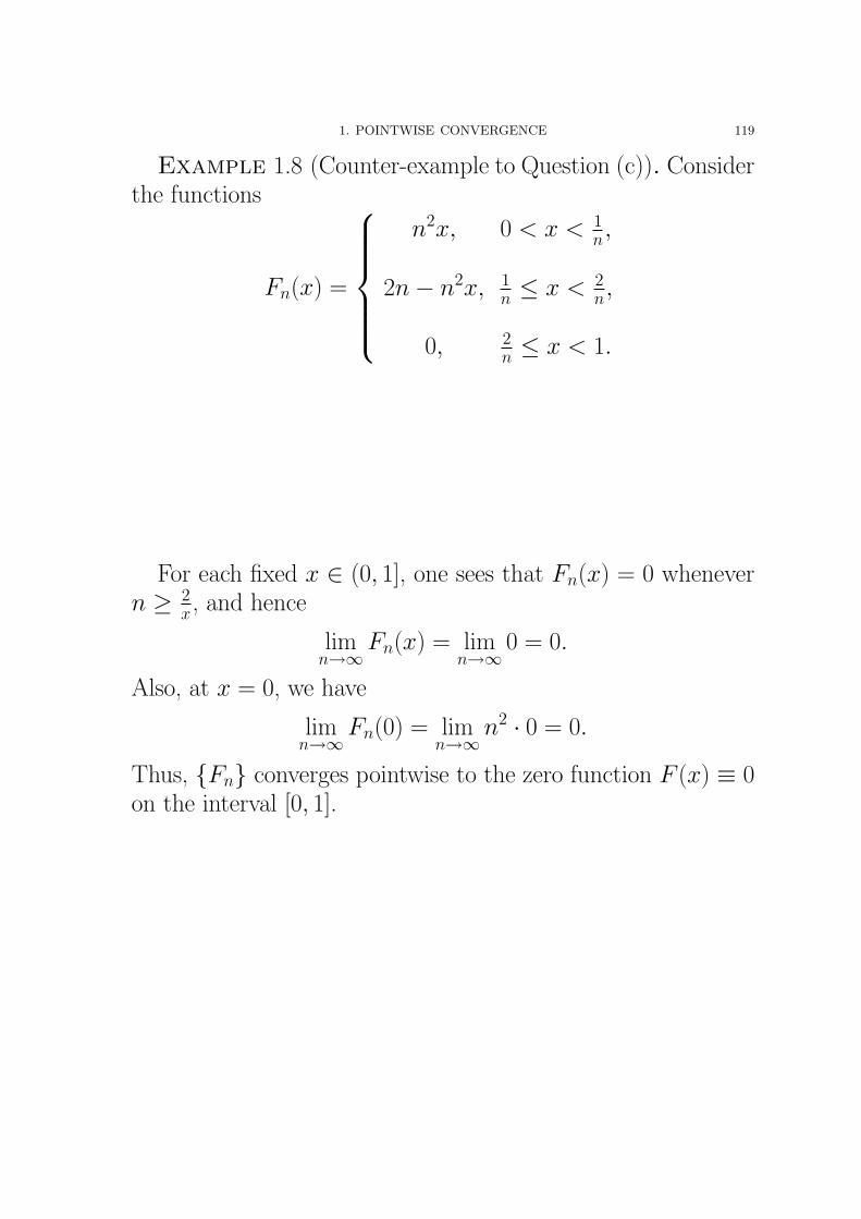
1. POINTWISE CONVERGENCE 119
Example 1.8 (Counter-example to Question (c)). Considerthe functions
Fn(x) =
n2x, 0 < x < 1
n,
2n− n2x, 1n ≤ x < 2
n,
0, 2n ≤ x < 1.
For each fixed x ∈ (0, 1], one sees that Fn(x) = 0 whenevern ≥ 2
x, and hence
limn→∞
Fn(x) = limn→∞
0 = 0.
Also, at x = 0, we have
limn→∞
Fn(0) = limn→∞
n2 · 0 = 0.
Thus, {Fn} converges pointwise to the zero function F (x) ≡ 0on the interval [0, 1].

120 3. SEQUENCES AND SERIES OF FUNCTIONS
For each n ≥ 1, we have∫ 1
0
Fn(x) dx =
∫ 1/n
0
n2x dx +
∫ 2/n
1/n
(2n− n2x) dx +
∫ 1
2/n
0 dx
=n2x2
2
∣∣∣∣ 1n0
+
(2nx− n2x2
2
)∣∣∣∣ 2n1n
+ 0
=1
2+ (4− 2)− (2− 1
2) + 0 = 1.
Thus we have
limn→∞
∫ 1
0
Fn(x) dx = limn→∞
1 = 1 6= 0 =
∫ 1
0
F (x) dx, i.e.
limn→∞
∫ 1
0
Fn(x) dx 6=∫ 1
0
(lim
n→∞Fn(x)
)dx.
Reason: At different x, Fn(x) converges to F (x) at differentpace (more specifically, in the definition of pointwise conver-gence, the choice of N depends on both ε and x).
2. UNIFORM CONVERGENCE 121
2. Uniform Convergence
We define a slightly different concept of convergence.
2.1. Uniform Convergence of Sequences of Func-tions.
Definition 2.1. {Fn} is said to converge uniformly toa function F on a set I if for every ε > 0, there exists an N(which depends only on ε) such that
|Fn(x)− F (x)| < ε
for ALL x ∈ I whenever n > N .
Remark 2.2. If {Fn} converges uniformly to F onI, then {Fn} converges pointwise to F on I. Con-versely, if {Fn} converges pointwise to F on I, then{Fn} need not converge uniformly to F on I.

122 3. SEQUENCES AND SERIES OF FUNCTIONS
The inequality in the definition can be expressed as
F (x)− ε < Fn(x) < F (x) + ε
for all x ∈ I and n > N . The geometric interpretation is thatfor n > N the graph of y = Fn(x) lies in the band spannedby the curves y = F (x) − ε and y = F (x) + ε, that is, givenany ε > 0 the graph of y = Fn(x) eventually lies in the bandspanned by the curves y = F (x)− ε and y = F (x) + ε.
Example 2.3. The sequence of function Fn = xn convergespointwise to 0 on [0, 1).
But from the graph we can see that the graph of Fn = xn
DOES NOT eventually lie in the band spanned by y = −ε andy = +ε. The geometric reason also tells us that {xn} does notconverge uniformly on [0, 1).
2. UNIFORM CONVERGENCE 123
2.2. Two Criteria for Uniform Convergence of {Fn}.The following theorem is useful (computationally) in determin-ing whether a sequence of functions converges uniformly or not.
Theorem 2.4 (T -test). Suppose {Fn} is a sequence offunctions converging pointwise to a function F on a set I,and let
Tn = supx∈I
|Fn(x)− F (x)|.
Then {Fn} converges uniformly to F on I if andonly if lim
n→0Tn = 0.
124 3. SEQUENCES AND SERIES OF FUNCTIONS
Proof. First we prove the ‘only if’ part. Suppose that {Fn}converges uniformly to F on I . Then for any given ε > 0, thereexists N such that
|Fn(x)− F (x)| < ε
2for all n > N and x ∈ I
=⇒ Tn = supx∈I
|Fn(x)− F (x)| ≤ ε
2< ε for all n > N
=⇒ |Tn − 0| = Tn < ε for all n > N.
Hence we have limn→0
Tn = 0.
Next we prove the ‘if’ part. Suppose that limn→0
Tn = 0.
Then for any given ε > 0, there exists N such that
|Tn − 0| = Tn < ε for all n > N
=⇒ supx∈I
|Fn(x)− F (x)| < ε for all n > N
=⇒ |Fn(x)− F (x)| < ε for all n > N and x ∈ I.
Hence {Fn} converges uniformly to F on I . This finishesthe proof of the theorem. �
2. UNIFORM CONVERGENCE 125
Theorem 2.5 (Cauchy’s Criterion). A sequence offunctions {Fn} converges uniformly on a set I ifand only if given any ε > 0, there exists a naturalnumber N such that(5)|Fn(x)− Fm(x)| < ε for all x ∈ I and all m,n > N.
Remark: Here N does not depend on x.
126 3. SEQUENCES AND SERIES OF FUNCTIONS
Proof. First we prove the ‘only if’ part. Suppose that {Fn}converges uniformly to the function F on I .
Then given any ε > 0, there exists N such that
|Fn(x)− F (x)| < ε
2for all x ∈ I and all n > N.
Then for all x ∈ I and m, n > N ,
|Fn(x)− Fm(x)| = |(Fn(x)− F (x))− (Fm(x)− F (x))|
≤ |Fn(x)− F (x)| + |Fm(x)− F (x)| < ε
2+
ε
2= ε.
This finishes the proof of the ‘only if’ part.
Next we prove the ‘if’ part. Suppose that equation 5 holds.
Then for each fixed point x ∈ I , {Fn(x)} is a Cauchy se-quence of real numbers, and thus by Cauchy’s criterion for se-quences, the sequence of real numbers {Fn(x)} converges.
For each x ∈ I , we denote the limit by F (x) = limn→∞
Fn(x).
Then {F (x)}x∈I forms a function on I , which we denote by F .
Given any ε > 0, by equation 5, there exists N such that
|Fn(x)− Fm(x)| < ε
2for all x ∈ I and all m,n > N.
Then for each fixed x ∈ I and n > N , we have
|Fn(x)− F (x)| = |Fn(x)− limm→∞
Fm(x)|
= limm→∞
|Fn(x)− Fm(x)| ≤ limm→∞
ε
2=
ε
2< ε.
Thus {Fn} converges uniformly to F , and this finishes theproof of the ‘if’ part. �
2. UNIFORM CONVERGENCE 127
2.3. Examples.
Example 2.6. Show that Fn(x) =sin2 x
n, x ∈ (−∞, +∞),
converges uniformly.
Proof. The limiting function F (x) is
F (x) = limn→∞
sin2 x
n= 0
for all x ∈ (−∞, +∞). Since
Tn = supx∈(−∞,+∞)
|Fn(x)−F (x)| = supx∈(−∞,+∞)
∣∣∣∣sin2 x
n
∣∣∣∣ ≤ 1
n→ 0
as n → ∞, thus the sequence of functions {Fn(x} convergesuniformly on (−∞, +∞). �
128 3. SEQUENCES AND SERIES OF FUNCTIONS
Example 2.7. Determine whether the following sequencesof functions converge uniformly on the indicated interval.
(a) fn(x) =n2 ln x
xn, x ∈ [1, +∞);
(b) fn(x) =n2 ln x
xn, x ∈ [2, +∞).
Solution. Let f (x) = limn→∞
fn(x) = 0 for x ≥ 1.
(a). Tn = supx≥1
|fn(x)− 0| = supx≥1
n2 ln x
xn= sup
x≥1fn(x). From
f ′n(x) = n2 1
x· x−n − n3 ln x · x−n−1 =
n2 − n3 ln x
xn+1= 0,
we have n2 − n3 ln x = 0 or x = e1n . Observe that fn(x) is
monotone increasing for 1 ≤ x ≤ e1n and monotone decreasing
for x ≥ e1n . Thus
Tn = maxx≥1
fn(x) = fn(e1n) =
n2 · 1n(
e1n
)n =n
e6→ 0
as n →∞ and so {fn(x)} does NOT converge uniformly.
(b). Since e1n ≤ 2 for n ≥ 2, the function fn(x) is monotone
decreasing on [2, +∞) for n ≥ 2 and so Tn = supx≥2
|fn(x) −
f (x)| = fn(2) =n2 ln 2
2nfor n ≥ 2. Since lim
n→∞Tn = 0, {fn}
converges uniformly on [2, +∞). �
2. UNIFORM CONVERGENCE 129
Example 2.8. Show that Fn(x) =n2 ln x sin nx
xnconverges
uniformly on [2, +∞).
Solution. F (x) = limn→∞
Fn(x) = 0 for x ≥ 2. Observe
Tn = supx≥2
|Fn(x)− F (x)| = supx≥2
n2 ln x| sin nx|xn
≤ n2 ln 2
2n
for n ≥ 2. Since limn→∞
Tn = 0, {Fn} converges uniformly. �
Remark. Let {Fn} be a sequence of functions on an intervalI . To see whether {Fn} is uniformly convergent, we may tryto do by the following steps.
(1). Determine the limiting function F (x) = limn→∞
Fn(x).
(2). Determine Tn = supx∈I
|Fn(x)− F (x)|.
(3). Check whether limn→∞
Tn = 0.
If Tn is difficult to be determined, then we may try to estimatean upper bound of Tn ( a lower bound of Tn if we guess thatthe sequence of functions might not be uniformly convergent).

130 3. SEQUENCES AND SERIES OF FUNCTIONS
2.4. Uniform Convergence of Series of Functions.
Definition 2.9.
∞∑n=1
fn is said to converge uniformly
(to S) on I if the sequence of its partial sums {Sn} convergesuniformly (to S) on I .
Theorem 2.10 (T -test for Series of Functions). Suppose∞∑
n=1
fn(x) is a series of functions converging pointwise on a
set I, and let
Tn = supx∈I
∣∣∣∣∣∞∑
k=n+1
fk(x)
∣∣∣∣∣ .Then
∞∑n=1
fn(x) converges uniformly on I if and only
if limn→∞
Tn = 0.
Proof. Let Sn(x) =
n∑k=1
fk(x) and S(x) =
∞∑k=1
fk(x).
Then
|Sn(x)− S(x)| =
∣∣∣∣∣∞∑
k=n+1
fk(x)
∣∣∣∣∣and so the T -test, Theorem 2.4, applies. �
2. UNIFORM CONVERGENCE 131
Theorem 2.11 (Cauchy Criterion). A series of func-
tions∞∑
n=1
fn converges uniformly on a set I if and
only if given any ε > 0, there exists a natural num-ber N such that∣∣∣∣∣
m∑k=n+1
fk(x)
∣∣∣∣∣ < ε for all x ∈ I and all m > n > N.
Remark: Here N does not depend on x.
Proof. The proof follows by applying the Cauchy Criterion
to the partial sums Sn(x) =
n∑k=1
fk(x). �
132 3. SEQUENCES AND SERIES OF FUNCTIONS
The following test is very useful in verifying that certainseries of functions converge uniformly to some functions on aninterval.
Theorem 2.12 (Weierstrass M -test). Consider a se-
ries of functions∞∑
k=1
fk on a set I. Suppose that
(i) |fk(x)| ≤ Mk for all x ∈ I, k = 1, 2, · · · , and
(ii)∞∑
k=1
Mk converges.
Then∞∑
k=1
fk converges uniformly (to some func-
tion) on I.
Remark. Weierstrass M -test only states that if a series offunctions satisfies conditions (i) and (ii), it converges uniformlyon I . If a series of functions does not satisfy these two con-ditions, the test fails, namely, no conclusion that you canclaim from this test.
2. UNIFORM CONVERGENCE 133
Proof. Since
∞∑k=1
Mk converges (by (ii)), by the Cauchy
Criterion, given any ε > 0, there exists N such thatm∑
k=n+1
Mk =
∣∣∣∣∣m∑
k=n+1
Mk
∣∣∣∣∣ < ε for all m > n > N
because Mk ≥ 0.
Then for all x ∈ I , we have∣∣∣∣∣m∑
k=n+1
fk(x)
∣∣∣∣∣ ≤m∑
k=n+1
|fk(x)| ≤m∑
k=n+1
Mk < ε.
Thus, by the Cauchy criterion,
∞∑k=1
fk converges uniformly
on I . �
134 3. SEQUENCES AND SERIES OF FUNCTIONS
2.5. Examples.
Example 2.13. Show that∞∑
n=1
cosn x
n2 + xconverges uniformly
on (0,∞).
Proof. Since ∣∣∣∣ cosn x
n2 + x
∣∣∣∣ ≤ 1
n2
for all x ∈ (0,∞) and the series
∞∑n=1
1
n2is convergent by the
p-series, the series of functions
∞∑n=1
cosn x
n2 + xconverges uniformly
by the Weierstrass M -test and hence the result. �
2. UNIFORM CONVERGENCE 135
Example 2.14. Does the series of functions∞∑
n=1
n2xn sin nx
converge uniformly on the interval [0, 12]? Justify your an-
swer.
Solution. Note that∣∣∣n2xn sin nx∣∣∣ ≤ n2
2n
for x ∈ [0, 12]. Since
limn→∞
(n + 1)2
2n+1
n2
2n
= limn→∞
(n + 1)2
2n2=
1
2< 1,
the series
∞∑n=1
n2
2nconverges, by the ratio test,
and so the series of functions∞∑
n=1
n2xn sin nx
converges uniformly on [0, 12] by the Weierstrass M -test. �
136 3. SEQUENCES AND SERIES OF FUNCTIONS
Example 2.15. Show that the series∞∑
n=1
(−1)n+1xn
ncon-
verges uniformly on [0, 1].
Note. The M -test fails for this example because
supx∈[0,1]
∣∣∣∣(−1)n+1xn
n
∣∣∣∣ =1
n
and
∞∑n=1
1
ndiverges. In this case, we use T -test or Cauchy
Criterion.
Proof. Let an(x) =xn
n. Then, for 0 ≤ x ≤ 1, we have
a1(x) ≥ a2(x) ≥ · · · ≥ 0 and limn→∞
an(x) = 0.
Thus the series
∞∑n=1
(−1)n+1xn
nconverges pointwise on [0, 1] by
the Alternating Series Test.
By the Alternating Series Estimation,
Tn = sup0≤x≤1
∣∣∣∣∣∞∑
k=n+1
(−1)k+1xk
k
∣∣∣∣∣ ≤ sup0≤x≤1
xn+1
n + 1=
1
n + 1.
Since limn→∞
1
n + 1= 0, the series (−1)n+1x
n
nconverges uni-
formly by the T -test. �

2. UNIFORM CONVERGENCE 137
Example 2.16. Show that the series∞∑
n=1
xn
ndoes not con-
verge uniformly on [0, 1).
Proof. Observe that
Tn = sup0≤x<1
|Sn(x)−S(x)| = sup0≤x<1
∣∣∣∣∣∞∑
k=n+1
xk
k
∣∣∣∣∣ = sup0<x<1
∞∑k=n+1
xk
k.
= sup0<x<1
(xn+1
n + 1+
xn+2
n + 2+ · · ·
)≥ sup
0<x<1
(xn+1
n + 1+
xn+2
n + 2+ · · · + x2n
2n
)=
1
n + 1+
1
n + 2+ · · · + 1
2n
(becausexk
kmonotone increasing on (0, 1))
≥ 1
2n+
1
2n+ · · · + 1
2n= n · 1
2n=
1
2.
Thus the sequence {Tn} does not tend to 0 and so the series
of functions
∞∑k=1
xk
kdoes NOT converge uniformly on [0, 1) by
the T -test. �
138 3. SEQUENCES AND SERIES OF FUNCTIONS
3. Uniform Convergence of {Fn} and Continuity
In this section we will prove that the limit of uniformly con-vergent sequence of continuous functions is again continuous.
Theorem 3.1. Let {Fn} be a sequence of continu-ous functions on an interval I. Suppose that {Fn}converges uniformly to a function F on I. ThenF is continuous on I.
Proof. Fix any point x0 ∈ I . We are going to show thatF is continuous at the point x0.
Given any ε > 0, since {Fn} converges uniformly to F on I ,there exists N such that
|Fn(x)− F (x)| < ε
3for all x ∈ I and all n > N.
Next we fix an n > N (say, n = [N ] + 1). Since Fn iscontinuous at x0, there exists δ > 0 (here δ depends on x0 andε) such that for all x satisfying |x− x0| < δ, we have
|Fn(x)− Fn(x0)| <ε
3.
Then for all x satisfying |x− x0| < δ, we have
|F (x)−F (x0)| = |F (x)−Fn(x)+Fn(x)−Fn(x0)+Fn(x0)−F (x0)|≤ |F (x)− Fn(x)| + |Fn(x)− Fn(x0)| + |Fn(x0)− F (x0)|
<ε
3+
ε
3+
ε
3= ε.
Thus F is continuous at x0. Since x0 is arbitrary, it fol-lows that F is continuous on I . This finishes the proof of thetheorem. �
3. UNIFORM CONVERGENCE OF {Fn} AND CONTINUITY 139
Example 3.2. Find the pointwise limit F of the sequence
Fn(x) =x2n
1 + x2n, x ∈ [0, 1].
Show using Theorem 3.1 that the convergence is not uni-form.
Solution. If 0 ≤ x < 1, we have
limn→∞
Fn(x) = limn→∞
x2n
1 + x2n=
0
1 + 0= 0.
If x = 1, then Fn(1) =1
2. Thus the limiting function F (x) is
F (x) =
0 0 ≤ x < 1
12 x = 1
Because each Fn(x) is continuous but F (x) is not, the sequenceof functions {Fn(x)} does not converge uniformly on [0, 1] byTheorem 3.1. �
It is possible that each Fn and F (x) = limn→∞
Fn(x) are con-
tinuous on an interval I , but {Fn} does not converge uniformlyto F (x).
For the case that I is not closed, an example can be given byI = [0, 1), Fn(x) = xn. (In this case F (x) = lim
n→∞Fn(x) = 0
for x ∈ I .)
For the case that I is a closed interval, an example can begiven as follows.
140 3. SEQUENCES AND SERIES OF FUNCTIONS
Example 3.3. Let Fn(x) = nxe−nx2. Show that
1) Each Fn(x) is continuous on I = [0, 1].2) {Fn(x)} converges pointwise to a continuous function
on I.3) {Fn(x)} does not converge uniformly on I.
Proof. Each Fn(x) is continuous because it is a well-definedelementary function on [0, 1].
Let F (x) = limn→∞
Fn(x) on [0, 1]. When x = 0, Fn(0) = 0 for
each n and F (0) = limn→∞ 0 = 0, when x 6= 0 (fixed),
F (x) = limn→∞
Fn(x) = limn→∞
nxe−nx2= lim
n→∞
nx
enx2
= limn→∞
x
enx2 · x2= lim
n→∞
1
xenx2 = 0.
Thus F (x) = 0 is continuous on [0, 1].Now Tn = sup
0≤x≤1|Fn(x)− F (x)| = sup
0≤x≤1Fn(x). From
F ′n(x) = ne−nx2
+ nxe−nx2 · (−2nx) = ne−nx2(1− 2nx2) = 0,
we have x = ±√
1
2n. Since Fn(0) = 0 and Fn(1) = ne−n,
sup0≤x≤1
Fn(x) = max0≤x≤1
Fn(x) = max
{0,
n
en, n · 1√
2n· e−n· 1
2n
}=
√n
2e.
Thus Tn =
√n
2e. Since lim
n→∞Tn = +∞, the sequence {Fn}
does not converge uniformly to F (x) on [0, 1]. �
3. UNIFORM CONVERGENCE OF {Fn} AND CONTINUITY 141
Corollary 3.4. Suppose that∞∑
k=1
fk converges uni-
formly to a function S on an interval I. Supposethat each fk is continuous on I. Then S is alsocontinuous on I.
Proof. Consider the sequence of partial sums {Sn} on I ,
where we have Sn =
n∑k=1
fk. Then {Sn} converges uniformly
to S on I . If each fk is continuous on I , then each Sn is alsocontinuous on I . Then by Theorem 3.1, S is also continuouson I . �
142 3. SEQUENCES AND SERIES OF FUNCTIONS
Example 3.5. Is∞∑
n=1
x
n2enx, x ∈ (0,∞), a continuous
function?
Solution. Let fn(x) =x
n2enx.
We find an upper bound of fn(x). Observe that
f ′n(x) =( x
n2enx
)′=
(xe−nx
n2
)′=
e−nx − nxe−nx
n2
=
e−nx
(1
n− x
)n
.
Thus f ′n(x) > 0 for 0 < x < 1n and f ′n(x) < 0 for x >
1n. It follows that fn(x) is monotone increasing on (0, 1
n] andmonotone decreasing on [1n, +∞). Hence
sup0<x<+∞
fn(x) = max0<x<+∞
fn(x) = fn
(1
n
)=
1n
n2en· 1n=
1
en3.
Let Mn =1
en3. Then |fn(x)| ≤ Mn for x ∈ (0,∞).
Since
∞∑n=1
Mn converges by the p-series, the series of functions
∞∑n=1
x
n2enxconverges uniformly by Weierstrass M -test on (0,∞).
According to Corollary 3.4, the function
∞∑n=1
x
n2enxis contin-
uous on (0,∞). �
3. UNIFORM CONVERGENCE OF {Fn} AND CONTINUITY 143
It is possible that each fn and
∞∑n=1
fn are continuous, but
∞∑n=1
fn does not converge uniformly.
Example 3.6. Consider the geometric series∞∑
n=0
xn = 1 + x + x2 + · · · =1
1− x
for−1 < x < 1. In this case, each xn and
∞∑n=0
xn are continuous
on I = (0, 1). We show that
∞∑n=0
xn does not converge uniformly
by T -test.
Since
Tn = sup−1<x<1
∣∣xn+1 + xn+2 + · · ·∣∣ ≥ sup
0≤x<1
∣∣xn+1 + xn+2 + · · ·∣∣
= sup0≤x<1
(xn+1 + xn+2 + · · ·
)≥ sup
0≤x<1xn+1 = 1,
the sequence {Tn} does not tend to 0
and so the series
∞∑n=0
xn does not converge uniformly on
(−1, 1) by the T -test. �
144 3. SEQUENCES AND SERIES OF FUNCTIONS
4. Uniform Convergence and Integration
Before we go on, we first recall some facts about Riemannintegrals (Reference: Our Text Book [2, Chapter 6, pp. 208-216]).
4.1. Review of Riemann Integration. Let f be abounded function on a finite interval [a, b]. A partition Pof [a, b] is a set of points {x0, x1, · · · , xn} such that
a = x0 < x1 < x2 < · · · < xn = b.
For such a partition P and i = 1, 2, · · ·n, we denote
Mi(f ) = supx∈[xi−1,xi]
f (x)
mi(f ) = infx∈[xi−1,xi]
f (x).
The upper (Riemann) sum of f with respect to thepartition P is defined to be
U(P, f ) :=
n∑i=1
Mi(f )∆xi.
Here ∆xi = xi−xi−1. Similarly the lower (Riemann) sumof f with respect to P is defined to be
L(P, f ) :=
n∑i=1
mi(f )∆xi.
4. UNIFORM CONVERGENCE AND INTEGRATION 145
The upper and lower integrals of f , denoted by
∫ b
a
f (x), dx
and
∫ b
a
f (x), dx, respectively, are defined by
∫ b
a
f (x) dx = inf{U(P, f ) | P is a partition of [a, b]},∫ b
a
f (x) dx = sup{L(P, f ) | P is a partition of [a, b]}.
Remark. If f is bounded, then∫ b
a
f (x) dx ≤∫ b
a
f (x) dx,
see [2, Theorem 6.1.4, p.211].
A function f is said to be Riemann integrable on [a, b]if ∫ b
a
f (x) dx =
∫ b
a
f (x) dx.
The common value is called the Riemann integral of f over[a, b], and it is denoted by
∫ b
a
f (x) dx =
∫ b
a
f (x) dx =
∫ b
a
f (x) dx.
146 3. SEQUENCES AND SERIES OF FUNCTIONS
Remark. In the following, (1) and (2) are from [2, Theorem6.1.8].
1) Any continuous function on a finite interval [a, b] is Rie-mann integrable.
2) Any monotone function on a finite interval [a, b] is Rie-mann integrable.
3) Any elementary function is continuous on its domain.
The elementary functions are the polynomials, ratio-nal functions, power functions (xa), exponential functions (ax),logarithmic functions, trigonometric and inverse trigonometricfunctions, hyperbolic and inverse hyperbolic functions, and allfunctions that can be obtained from these by five operationsof addition, subtraction, multiplication, division, and composi-tion.

4. UNIFORM CONVERGENCE AND INTEGRATION 147
4.2. The Theorems.
Theorem 4.1. Let {Fn} be a sequence of Riemannintegrable functions on a finite interval [a, b]. Sup-pose that {Fn} converges uniformly to a functionF on [a, b]. Then F is Riemann integrable on [a, b],and
limn→∞
∫ b
a
Fn(x) dx =
∫ b
a
F (x) dx
i.e. limn→∞
∫ b
a
Fn(x) dx =
∫ b
a
(lim
n→∞Fn(x)
)dx.
148 3. SEQUENCES AND SERIES OF FUNCTIONS
Proof. By definition, given any ε > 0, there exists N suchthat
|Fn(x)− F (x)| < ε
2(b− a)
for all n > N and x ∈ [a, b]. Thus
Fn(x)− ε
2(b− a)< F (x) < Fn(x) +
ε
2(b− a)
for all x ∈ [a, b] and n > N .
It follows that
(6)
∫ b
a
(Fn(x)− ε
2(b− a)
)dx ≤
∫ b
a
F (x) dx
≤∫ b
a
F (x) dx ≤∫ b
a
(Fn(x) +
ε
2(b− a)
)dx
for n > N .
Since Fn(x) is Riemann integrable, we have∫ b
a
(Fn(x)− ε
2(b− a)
)dx =
∫ b
a
(Fn(x)− ε
2(b− a)
)dx
=
∫ b
a
Fn(x) dx− ε
2(b− a)· (b− a) =
∫ b
a
Fn(x) dx− ε
2,∫ b
a
(Fn(x) +
ε
2(b− a)
)dx =
∫ b
a
(Fn(x) +
ε
2(b− a)
)dx
=
∫ b
a
Fn(x) dx +ε
2(b− a)· (b− a) =
∫ b
a
Fn(x) +ε
2.
4. UNIFORM CONVERGENCE AND INTEGRATION 149
Together with Inequality (6), we obtain
(7)
∫ b
a
Fn(x) dx− ε
2≤∫ b
a
F (x) dx
≤∫ b
a
F (x) dx ≤∫ b
a
Fn(x) dx +ε
2for n > N . It follows that
0 ≤∫ b
a
F (x) dx−∫ b
a
F (x) dx ≤ ε.
Let ε → 0, we have∫ b
a
F (x) dx−∫ b
a
F (x) dx = 0
and so F (x) is Riemann integrable.
From Inequality (7), we have∫ b
a
Fn(x) dx− ε
2≤∫ b
a
F (x) dx ≤∫ b
a
Fn(x) dx+ε
2, that is,∣∣∣∣∫ b
a
Fn(x) dx−∫ b
a
F (x) dx
∣∣∣∣ ≤ ε
2< ε
for n > N and hence
limn→∞
∫ b
a
Fn(x) dx =
∫ b
a
F (x) dx.
�
150 3. SEQUENCES AND SERIES OF FUNCTIONS
Example 4.2. Compute, justifying your answer,
limn→∞
∫ 1
0
sin nx
n + x2dx.
Solution. Let Fn(x) =sin nx
n + x2. Then the limiting func-
tion
F (x) = limn→∞
Fn(x) = limn→∞
sin nx
n + x2= 0
for any given 0 ≤ x ≤ 1, by the Squeeze theorem, because
−1
n≤ sin nx
n + x2≤ 1
n
and limn→∞
1
n= − lim
n→∞
1
n= 0. Since
Tn = sup0≤x≤1
|Fn(x)− F (x)| = sup0≤x≤1
∣∣∣∣ sin nx
n + x2
∣∣∣∣ ≤ 1
n,
limn→∞
Tn = 0 by the Squeeze Theorem and so the sequence of
functions {Fn} converges uniformly to F (x). Thus
limn→∞
∫ 1
0
sin nx
n + x2dx =
∫ 1
0
limn→∞
sin nx
n + x2dx =
∫ 1
0
0 dx = 0.
�
4. UNIFORM CONVERGENCE AND INTEGRATION 151
Corollary 4.3. Suppose that∞∑
k=1
fk converges uni-
formly to a function S on a finite interval [a, b].Suppose that each fk is a Riemann integrable func-tion on [a, b]. Then S is also Riemann integrableon [a, b], and∫ b
a
S(x) dx =
∞∑k=1
∫ b
a
fk(x) dx,
i.e.
∫ b
a
∞∑k=1
fk(x) dx =
∞∑k=1
∫ b
a
fk(x) dx.
Proof. Consider the sequence of partial sums {Sn} on [a, b],
where Sn =
n∑k=1
fk. Then {Sn} converges uniformly to S on
[a, b]. If each fk is Riemann integrable on [a, b], then each Sn
is also Riemann integrable on [a, b]. Then by Theorem 4.1, Sis also Riemann integrable on [a, b], and∫ b
a
S(x) dx = limn→∞
∫ b
a
Sn(x) dx = limn→∞
∫ b
a
n∑k=1
fk(x) dx
= limn→∞
n∑k=1
∫ b
a
fk(x) dx =
∞∑k=1
∫ b
a
fk(x) dx.
�
152 3. SEQUENCES AND SERIES OF FUNCTIONS
By using this theorem, we have the following amazing for-mula.
Example 4.4. Show that
ln 2 =
∞∑n=1
1
n · 2n=
1
2+
1
2 · 22+
1
3 · 23+ · · ·
Proof. Since∣∣xn−1
∣∣ ≤ (1
2
)n−1
for 0 ≤ x ≤ 1
2and
the geometric series
∞∑n=0
(1
2
)n−1
converges, the series
∞∑n=1
xn−1
converges uniformly to1
1− xon [0, 1
2] by the Weierstrass M -
test. Thus we have∫ 12
0
1
1− x=
∫ 12
0
∞∑n=1
xn−1 dx
=
∞∑n=1
∫ 12
0
xn−1 dx =
∞∑n=1
xn
n
∣∣∣∣1/20
=
∞∑n=1
1
n · 2n.
Since∫ 12
0
1
1− x= − ln(1−x)
∣∣∣120
= − ln
(1− 1
2
)= − ln
(1
2
)= ln 2,
we obtain the formula
ln 2 =
∞∑n=1
1
n · 2n=
1
2+
1
2 · 22+
1
3 · 23+ · · · .
�
4. UNIFORM CONVERGENCE AND INTEGRATION 153
Remark 4.5. Example 4.4 gives a way to estimate the num-ber ln 2 because the remainder
Rn =
∞∑k=n+1
1
k · 2k=
1
(n + 1)2n+1+
1
(n + 2)2n+2+ · · ·
<1
(n + 1)2n+1+
1
(n + 1)2n+2+
1
(n + 1)2n+3+ · · ·
=1
(n + 1)2n+1
(1 +
1
2+
1
22+ · · ·
)=
1
(n + 1)2n+1· 1
1− 12
=1
(n + 1)2n.
For instance,
ln 2 ≈ 1
2+
1
2 · 22+
1
3 · 23+ · · · + 1
10 · 210
with error less than1
11 · 210=
1
11264.
154 3. SEQUENCES AND SERIES OF FUNCTIONS
4.3. Remarks on Theorem 4.1. For completeness weinclude the following result, which does not require uniformconvergence. The proof requires new theory called Lebesgueintegration. There are applications in the area of probabilityand statistics.
Theorem 4.6 (Bounded Convergence Theorem). Let {Fn}be a sequence of Riemann integrable functions con-verging pointwise to F (x) on [a, b]. Suppose that
(i) F (x) is Riemann integrable, and(ii) there exists a positive constant M such that
|Fn(x)| ≤ M
for all x ∈ [a, b] and n ∈ N.
Then
limn→∞
∫ b
a
Fn(x) dx =
∫ b
a
F (x) dx =
∫ b
a
limn→∞
Fn(x) dx
5. UNIFORM CONVERGENCE AND DIFFERENTIATION 155
5. Uniform Convergence and Differentiation
Theorem 5.1. Let {Fn} be a sequence of functions on[a, b] such that
(i) each F ′n exists and is continuous on [a, b],
(ii) {Fn} converges pointwise to a function F on [a, b],and
(iii) {F ′n} converges uniformly on [a, b].
Then F is differentiable on [a, b], and for all x ∈ [a, b],
F ′(x) = limn→∞
F ′n(x),
i.e.d
dx
(lim
n→∞Fn(x)
)= lim
n→∞
(d
dxFn(x)
).
Remark. Here the differentiability and continuity at the end-points a and b refer to the one sided derivatives and limitsrespectively.

156 3. SEQUENCES AND SERIES OF FUNCTIONS
Proof. By (iii), {F ′n} converges uniformly to a function,
denoted by g, on [a, b], where
g(x) = limn→∞
F ′n(x)
for all x ∈ [a, b].
By (i), since each F ′n is continuous on [a, b], F ′
n is also Rie-mann integrable on [a, b], and by the fundamental theorem ofcalculus,∫ x
a
F ′n(t) dt = Fn(x)− Fn(a) for all x ∈ [a, b].
Letting n →∞, for all x ∈ [a, b],
(8) limn→∞
∫ x
a
F ′n(t) dt = lim
n→∞
(Fn(x)−Fn(a)
)= F (x)−F (a).
On the other hand, since {F ′n} converges uniformly to g on
[a, b], it follows from Theorem 4.1 that
limn→∞
∫ x
a
F ′n(t) dt =
∫ x
a
(lim
n→∞F ′
n(t))dt =
∫ x
a
g(t) dt.
Together with equation 8, it follows that
F (x)− F (a) =
∫ x
a
g(t) dt for all x ∈ [a, b].
5. UNIFORM CONVERGENCE AND DIFFERENTIATION 157
By (i) and Theorem 3.1, g is continuous on [a, b].
Then by the fundamental theorem of calculus, we have
d
dx
∫ x
a
g(t) dt = g(x).
Together with equation 8, it follows that F is also differen-tiable on [a, b],
and for all x ∈ [a, b],
d
dx
(F (x)− F (a)
)=
d
dx
∫ x
a
g(t) dt = g(x),
i.e.F ′(x) = g(x), i.e.d
dx
(lim
n→∞Fn(x)
)= lim
n→∞
( d
dxFn(x)
).
The proof is finished. �
158 3. SEQUENCES AND SERIES OF FUNCTIONS
Remark 5.2. By inspecting the proof, Theorem 5.1 stillholds when the closed interval [a, b] is replaced by (a, b),(a, b] or [a, b).
This theorem can be generalized as follows.
Theorem 5.3. Let {Fn} be a sequence of differen-tiable functions on [a, b] such that
(a) {Fn(x0)} converges for some x0 ∈ [a, b], and(b) {F ′
n} converges uniformly on [a, b].
Then {Fn} converges uniformly to a function F (x)on [a, b] with,
F ′(x) = limn→∞
F ′n(x), i.e.
d
dx
(lim
n→∞Fn(x)
)= lim
n→∞
( d
dxFn(x)
).
The proof of this theorem is omitted, see [2, Theorem 8.5.1,pp.340-341].
5. UNIFORM CONVERGENCE AND DIFFERENTIATION 159
Corollary 5.4. Let∞∑
k=1
fk be a series of differen-
tiable functions on [a, b] such that
(a)∞∑
k=1
fk(x0) converges for some x0 ∈ [a, b], and
(b)∞∑
k=1
f ′k converges uniformly on [a, b].
Then∞∑
k=1
fk converges uniformly to a function S(x)
on [a, b], and for all x ∈ [a, b],
S ′(x) =
∞∑k=1
f ′k(x), i.e.d
dx
( ∞∑k=1
fk(x))
=
∞∑k=1
d
dxfk(x).
Proof. Consider the partial sums Sn(x) =
n∑k=1
fk(x) on
[a, b]. By (a), {Sn(x0)} converges, and, by (b), {S ′n(x)} con-verges uniformly on [a, b]. By Theorem 5.3, {Sn(x)} converges
uniformly to a function S(x) on [a, b] and so
∞∑k=1
fk(x) con-
verges uniformly to S(x) on [a, b] by the definition. Further-more, by Theorem 5.3, for all x ∈ [a, b], S ′(x) = lim
n→∞S ′n(x),
that is,d
dx
( ∞∑k=1
fk(x))
= limn→∞
( n∑k=1
fk(x))′
= limn→∞
n∑k=1
f ′k(x) =
∞∑k=1
d
dxfk(x).
�
160 3. SEQUENCES AND SERIES OF FUNCTIONS
As an application, we give a proof of binomial series. Leta be any real number. The binomial number, a chooses n, isdefined by (
a
n
)=
a(a− 1)(a− 2) · · · (a− n + 1)
n!
for positive integers n. For instance,(12
1
)=
1
2,
(12
2
)=
12 ·(
12 − 1
)2!
= −1
8,(1
2
3
)=
12 ·(
12 − 1
) (12 − 2
)3!
=12 ·(−1
2
)·(−3
2
)6
=1
16.
We also use the convention that
(a
0
)= 1 for any a.
Theorem 5.5 (Binomial Series). Let a be any real con-stant. Then
(1+x)a = 1+ax+a(a− 1)
2!x2+· · · = 1+
∞∑n=1
(a
n
)xn =
∞∑n=0
(a
n
)xn
for |x| < 1.
5. UNIFORM CONVERGENCE AND DIFFERENTIATION 161
Proof. Let ρ be any fixed positive number with 0 < ρ < 1and let I = [−ρ, ρ]. Consider the series of functions
1 +
∞∑n=1
(a
n
)xn
converges when x = 0 ∈ [−ρ, +ρ]. So it satisfies condition(a) of Corollary 5.4. We check condition (b) of Corollary 5.4,namely, the series of functions
∞∑n=1
(a
n
)nxn−1
converges uniformly on [−ρ, +ρ]. Note that∣∣∣∣(a
n
)nxn−1
∣∣∣∣ ≤ ∣∣∣∣(a
n
)∣∣∣∣nρn−1
for x ∈ [−ρ, +ρ]. Let Mn =
∣∣∣∣(a
n
)∣∣∣∣nρn−1. Then
limn→∞
Mn+1
Mn= lim
n→∞
∣∣( an+1
)∣∣ (n + 1)ρn∣∣(an
)∣∣nρn−1
= limn→∞
|a| · |a− 1| · · · |a− n|(n + 1)!
· (n + 1) · ρn
|a| · |a− 1| · · · |a− n + 1|n!
· n · ρn−1
= limn→∞
|a| · |a− 1| · · · |a− n| · n! · (n + 1) · ρ(n + 1)! · |a| · |a− 1| · · · |a− n + 1| · n
= limn→∞
|a− n| · ρn
= limn→∞
|a/n− 1| · ρ = ρ < 1.
162 3. SEQUENCES AND SERIES OF FUNCTIONS
Thus the series
∞∑n=1
Mn converges and so the series of functions
∞∑n=1
(a
n
)nxn−1 converges uniformly on [−ρ, ρ], by the Weier-
strass M -test.
By Corollary 5.4, the series 1 +
∞∑n=1
(a
n
)xn converges uni-
formly to a function f (x) on [−ρ, ρ] with
f ′(x) =
∞∑n=1
(a
n
)nxn−1.
Next we are going to set up a differential equation that
(1 + x)f ′(x) = af (x).
(Note. Since the goal is to show that f (x) = (1 + x)a, thisequation is observed from that, if y = (1 + x)a, then y′ =a(1 + x)a−1 and so (1 + x)y′ = (1 + x)a = y.)
5. UNIFORM CONVERGENCE AND DIFFERENTIATION 163
f ′(x) =
∞∑n=1
(a
n
)nxn−1 =
∞∑n=1
a(a− 1) · · · (a− n + 1) · nn!
xn−1
=
∞∑n=1
a(a− 1) · · · (a− n + 1)
(n− 1)!xn−1 = a
∞∑n=1
(a− 1
n− 1
)xn−1 and
(1 + x)f ′(x) = f ′(x) + xf ′(x)
= a∞∑
n=1
(a− 1
n− 1
)xn−1 + a
∞∑n=1
(a− 1
n− 1
)xn
= a
∞∑n=0
(a− 1
n
)xn + a
∞∑n=1
(a− 1
n− 1
)xn
= a
{1 +
∞∑n=1
[(a− 1
n
)+
(a− 1
n− 1
)]xn
}
= a
[1 +
∞∑n=1
(a
n
)xn
]= af (x),
where (a− 1
n
)+
(a− 1
n− 1
)=
(a− 1)(a− 2) · · · (a− 1− n + 1)
n!
+(a− 1)(a− 2) · · · (a− 1− n + 2)
(n− 1)!
=(a− 1)(a− 2) · · · (a− 1− n + 2)
n!(a− 1− n + 1 + n)
=a(a− 1) · · · (a− n + 1)
n!=
(a
n
).
164 3. SEQUENCES AND SERIES OF FUNCTIONS
Our last step is to solve the differential equation
(1 + x)f ′(x) = af (x).
Let y = f (x). Then we obtain the differential equation
(1 + x)dy
dx= ay
dy
y=
a dx
1 + x
=⇒∫
dy
y=
∫a dx
1 + x=⇒ ln |y| = a ln |1 + x| + A = ln |1 + x|a + A
=⇒ |y| = eln |y| = eA|1 + x|a
=⇒ y = C|1 + x|a,where C = ±eA is a constant. By putting x = 0,
C = (1 + 0)a = y(0) = 1 +
∞∑n=1
(a
n
)0n = 1.
Thus y = |1 + x|a or
(1 + x)a = 1 +
∞∑n=1
(a
n
)xn
for |x| ≤ ρ because 1 + x > 0 when |x| ≤ ρ < 1. Since ρ isany number with 0 < ρ < 1, the formula
(1 + x)a = 1 +
∞∑n=1
(a
n
)xn
holds for all x ∈ (−1, 1). �
5. UNIFORM CONVERGENCE AND DIFFERENTIATION 165
For instance,
√1 + x = (1 + x)
12 =
∞∑k=0
(12
k
)xk
= 1 +1
2x +
(12
) (−1
2
)2!
x2 + · · ·√1− x3 = (1− x3)
12 =
∞∑k=0
(12
k
)(−x3
)k= 1− 1
2x3 +
(12
) (−1
2
)2!
x6 + · · ·
√4.1 =
(4 +
1
10
)12
= 2
(1 +
1
40
)12
= 2
∞∑k=0
(12
k
)(1
40
)k
.
Example 5.6. Evaluate√
4.1 with error less than 0.001.
Solution.
√4.1 =
(4 +
1
10
)12
= 2
(1 +
1
40
)12
= 2
∞∑k=0
(12
k
)(1
40
)k
.
= 2 + 2
∞∑k=1
(12
k
)(1
40
)k
.
166 3. SEQUENCES AND SERIES OF FUNCTIONS
Now (12
k
)=
12 ·(
12 − 1
)· · ·(
12 − k + 1
)k!
= (−1)k+112 ·(1− 1
2
)· · ·(k − 1
2 − 1)
k!for k ≥ 2. Let
bk =12 ·(1− 1
2
)· · ·(k − 1
2 − 1)
k!
(1
40
)k
.
Then, for k ≥ 2, we have bk ≥ 0,
bk+1
bk=
12 ·(1− 1
2
)· · ·(k − 1
2 − 1)·(k − 1
2
)(k + 1)!
(1
40
)k+1
12 ·(1− 1
2
)· · ·(k − 1
2 − 1)
k!
(1
40
)k
=k − 1
2
40(k + 1)≤ 1,
that is, b2 ≥ b3 ≥ · · · ≥ 0, and limk→∞
bk = 0 by the Squeeze
Theorem because
0 ≤ bk ≤12 · 1 · 2 · · · (k − 1)
k!
(1
40
)k
=1
2k · 40k
for k ≥ 2 and limk→∞
1
2k · 40k= 0.
5. UNIFORM CONVERGENCE AND DIFFERENTIATION 167
By the alternating series estimation, from
2 ·
∣∣∣∣∣( 1
2
k + 1
)(1
40
)k+1∣∣∣∣∣ < 0.001,
we have k ≥ 1, because 2b2 =1
6400< 0.001, and so
√4.1 ≈ 2 + 2
(12
1
)1
40= 2.025
with error less than 0.001. �
168 3. SEQUENCES AND SERIES OF FUNCTIONS
6. Power Series
6.1. Power Series.
Definition 6.1. A power series in x is of the form∞∑
n=0
anxn = a0 + a1x + a2x
2 + · · ·
Example 6.2. Below are some examples
1.
∞∑n=0
(n + 1)xn = 1 + 2x + 3x2 + 4x3 + 5x4 + · · ·
2.
∞∑n=0
xn
n!= 1 + x +
x2
2!+
x3
3!+ · · ·
6. POWER SERIES 169
Definition 6.3. A power series in x− x0 is of the form∞∑
n=0
an(x− x0)n = a0 + a1(x− x0) + a2(x− x0)
2 + · · ·
Example 6.4. Here are some examples.
1.
∞∑n=0
(x− 1)n = 1 + (x− 1) + (x− 1)2 + · · · .
2.
∞∑n=1
n2(x + 2)n = (x + 2) + 22(x + 2)2 + 32(x + 2)3 + · · · .
Warning. Don’t expand out the terms an(x − x0)n in the
power series
∞∑n=0
an(x−x0)n because, when you rearrange terms
in an (infinite) series, you may get different values. (For partialsums, you can expand out, if it is necessary, because there areonly finitely many terms.)
Question: Given a power series
∞∑n=0
an(x − x0)n, when does
it converge and when does it diverge? In other words, what is
the domain of the function
∞∑n=0
an(x − x0)n. We are going to
answer this question.
170 3. SEQUENCES AND SERIES OF FUNCTIONS
6.2. Radius of Convergence.
Definition 6.5. Given a power series∞∑
n=0
an(x − x0)n,
the radius of convergence R is defined by
R =1
limn→∞
n√|an|
.
If limn→∞
n√|an| = ∞, we take R = 0, and if lim
n→∞n√|an| = 0,
we set R = ∞. If limn→∞
|an+1||an|
exists, R is also given by
R =1
limn→∞
|an+1||an|
Remark. Recall that
limn→∞
|an+1||an|
≤ limn→∞
n√|an| ≤ lim
n→∞n√|an| ≤ lim
n→∞
|an+1||an|
.
If limn→∞
|an+1||an|
exists, then
limn→∞
|an+1||an|
= limn→∞
|an+1||an|
and so limn→∞
n√|an| exists with
limn→∞
n√|an| = lim
n→∞
|an+1||an|
.
6. POWER SERIES 171
Example 6.6. What is the radius of convergence for theseries
1 +x
3+
x2
42+
x3
33+
x4
44+
x5
35+
x6
46+ · · ·
Solution. Since
an =
1
42kn = 2k
1
32k−1n = 2k − 1,
we have
n√|an| =
1
4n = 2k
1
3n = 2k − 1.
Thus limn→∞
n√|an| =
1
3and so the radius of convergence
R =1
limn→∞
n√|an|
=113
= 3.
�
172 3. SEQUENCES AND SERIES OF FUNCTIONS
Example 6.7. Find the radius of convergence of the power
series∞∑
n=0
(4x + 3)n
n3
Solution. Observe that∞∑
n=1
(4x + 3)n
n3=
∞∑n=1
4n
n3·(
x +3
4
)n
.
Thus
R =1
limn→∞
|an+1||an|
=1
limn→∞
4n+1 · n3
(n + 1)3 · 4n
=1
limn→∞
4(1 + 1
n
)3 =1
4.
�
6. POWER SERIES 173
Theorem 6.8. Given any power series∞∑
k=0
ak(x − x0)k
with radius of convergence R, 0 ≤ R ≤ ∞, then the
series∞∑
k=0
ak(x− x0)k
(i) converges absolutely for all x with |x − x0| < R,and
(ii) diverges for all x with |x− x0| > R.
Remark: At the (two) end points |x − x0| = R, thatis, x = x0 ± R, the power series possibly converges andpossibly diverges.
174 3. SEQUENCES AND SERIES OF FUNCTIONS
Proof. By definition, the radius of convergence
R =1
limk→∞
|ak|1k
.
Assertion (i) follows from the root test because, from
limk→∞
∣∣ak(x− x0)k∣∣1k = lim
k→∞|ak|
1k ·|x−x0| = |x−x0|· lim
k→∞|ak|
1k
= |x− x0| ·1
R< R · 1
R< 1,
the series
∞∑k=0
∣∣ak(x− x0)k∣∣ converges.

6. POWER SERIES 175
Next we are going to prove (ii) by contradiction.
Suppose that
∞∑k=0
ak(x − x0)k converges at a point x with
|x− x0| > R.
Then by Theorem 1.7, we have
limk→∞
ak(x− x0)k = 0.
Let ε = 1. Then there exists N such that
|ak(x− x0)k − 0| < 1 for all k > N
=⇒ |ak(x− x0)k|
1k < 1 for all k > N
=⇒ |ak|1k <
1
|x− x0|for all k > N
=⇒ supn≥k
|ak|1k ≤ 1
|x− x0|for all n > N
=⇒ limk→∞
|ak|1k ≤ 1
|x− x0|
=⇒ 1
R≤ 1
|x− x0|<
1
R,
which is a contradiction.
Hence we must have
∞∑k=0
ak(x− x0)k diverges at each x sat-
isfying |x− x0| > R. �
176 3. SEQUENCES AND SERIES OF FUNCTIONS
6.3. Interval of convergence. In view of Theorem 6.8,
for a power series
∞∑k=0
ak(x − x0)k with radius of convergence
R, the set of points at which
∞∑k=0
ak(x−x0)k is convergent form
an interval called the interval of convergence, which mustbe either
(x0 −R, x0 + R), (x0 −R, x0 + R],
[x0 −R, x0 + R) or [x0 −R, x0 + R].
Example 6.9. Find the interval of convergence of thepower series.
(i)∞∑
n=1
(x− 2)n
n2(ii)
∞∑n=1
(x− 2)n
n(iii)
∞∑n=1
n(x− 2)n
Solution. (i). First we find the radius of convergence
R =1
limn→∞
|an+1||an|
=1
limn→∞
n2
(n + 1)2
=1
limn→∞
1
(1 + 1n)2
= 1.
Next we check the ending-points x0 ± R = 2 ± 1 = 1, 3.
When x = 1, the series is
∞∑n=1
(−1)n
n2, which is convergent by
Example 3.5. When x = 3, the series is
∞∑n=1
1
n2, which is con-
vergent by the p-series. Thus the interval of convergence is[1, 3].
6. POWER SERIES 177
(ii).
∞∑n=1
(x− 2)n
n.
The radius of convergence is
R =1
limn→∞
|an+1||an|
=1
limn→∞
n
(n + 1)
=1
limn→∞
1
(1 + 1n)
= 1.
Now we check the ending-points x0±R = 1, 3. When x = 1,
the series is
∞∑n=1
(−1)n
n, which is convergent by Example 3.5.
When x = 3, the series is
∞∑n=1
1
n, which is divergent by the
p-series. Thus the interval of convergence is [1, 3).
(iii).
∞∑n=1
n(x− 2)n.
The radius of convergence is
R =1
limn→∞
|an+1||an|
=1
limn→∞
n + 1
n
=1
limn→∞
(1 +
1
n
) = 1.
Now we check the ending-points x0±R = 1, 3. When x = 1,
the series is
∞∑n=1
n(−1)n, and when x = 3, the series is
∞∑n=1
n.
Both of these series are divergent by the divergence test. Thusthe interval of convergence is (1, 3). �
178 3. SEQUENCES AND SERIES OF FUNCTIONS
6.4. Uniform Convergence of Power Series.
Theorem 6.10 (Abel Theorem). Let∞∑
n=0
an(x− x0)n be a
power series, and let R ≥ 0.
(1). If∞∑
n=0
anRn converges,
then the series of functions∞∑
n=0
an(x− x0)n
converges uniformly on [x0, x0 + R].
(2). If∞∑
n=0
an(−R)n converges,
then the series of functions∞∑
n=0
an(x− x0)n
converges uniformly on [x0 −R, x0].
Remark. In this theorem, we do not assume that R is theradius of convergence.
6. POWER SERIES 179
Proof. We only prove assertion (1). The proof of assertion(2) is similar to.
We may assume that R > 0. Let t =x− x0
R. Then
∞∑n=0
an(x− x0)n =
∞∑n=0
anRntn.
We are going to show that this series converges uniformly on0 ≤ t ≤ 1, that is, x0 ≤ x ≤ x0 + R.
Write an for anRn. By the assumption, the series
∞∑n=0
an =
∞∑n=0
anRn converges.
Let An =
n∑k=0
ak −∞∑
k=0
ak = −∞∑
k=n+1
ak. Then
An − An−1 =
(−
∞∑k=n+1
ak
)−
(−
∞∑k=n
ak
)= an.
By Abel Partial Summation Formula, for 0 ≤ n < m, 0 ≤ t ≤1, ∣∣∣∣∣
m∑k=n+1
aktk
∣∣∣∣∣ =
∣∣∣∣∣Amtm − Antn+1 +
m−1∑k=n+1
Ak(tk − tk+1)
∣∣∣∣∣≤ |Am|tm + |An|tn+1 +
m−1∑k=n+1
|Ak| · tk(1− t).
180 3. SEQUENCES AND SERIES OF FUNCTIONS
Since
∞∑n=0
an converges, the remainders
∞∑k=n+1
ak = −An
tends to 0 and so limn→∞
An = 0. Given ε > 0, there exists
N such that|An| <
ε
2for n > N .
Now, for m > n > N and 0 ≤ t ≤ 1,∣∣∣∣∣m∑
k=n+1
aktk
∣∣∣∣∣ ≤ |Am|tm + |An|tn+1 +
m−1∑k=n+1
|Ak| · tk(1− t)
<ε
2tm +
ε
2tn+1 +
m−1∑k=n+1
ε
2· tk · (1− t)
=ε
2
(tm + tn+1 + (1− t)(tn+1 + tn+2 + · · · + tm−1)
)=
ε
2
(tm + tn+1 + (tn+1 + tn+2 + · · · + tm−1)
−(tn+2 + tn+3 + · · · + tm))
=ε
2· 2tn+1 ≤ ε.
By the Cauchy Criterion, the series of functions∞∑
n=0
antn =
∞∑n=0
an(x− x0)n
converges uniformly on 0 ≤ t ≤ 1, or on x0 ≤ x ≤ x0 +R. �

6. POWER SERIES 181
Theorem 6.11 (Uniform Convergence Theorem). Let∞∑
n=0
an(x− x0)n
be a power series of radius of convergence R > 0.Let I be the interval of convergence. Then the se-
ries of functions∞∑
n=0
an(x−x0)n converges uniformly
on any closed interval [c, d] ⊆ I.
Remark. (1). I = [x0 − R, x0 + R], [x0 − R, x0 + R),(x0 −R, x0 + R], or (x0 −R, x0 + R).
If I = [x0 − R, x0 + R], then the power series convergesuniformly on I .
In other cases, since I is not closed, the theorem says thatthe power series converges uniformly on any closed sub-interval of I .
For instance, if x0 = 0, R = 1, and I = [−1, 1), then thepower series converges uniformly on [−1, 0.9], [0, 0.9] and etc,but it need not converge uniformly on [−1, 1) or [0, 1).
(2). In any of the four cases, the power series converges uni-formly on any closed sub-interval of (x0 −R, x0 + R).
182 3. SEQUENCES AND SERIES OF FUNCTIONS
Proof. There are three cases: (i). c ≤ x0 ≤ d, (ii). x0 <c ≤ d, or (iii). c ≤ d < x0.
Case (i). c ≤ x0 ≤ d. Since∞∑
n=0
an(d− x0)n and
∞∑n=0
an(c− x0)n
converges because c, d ∈ I , where d− x0 ≥ 0 and c− x0 ≤ 0,the power series
∞∑n=0
an(x− x0)n
converges uniformly on c ≤ x ≤ x0] and x0 ≤ x ≤ d by theAbel theorem
and so on the union [c, d] = [c, x0] ∪ [x0, d].
Case (ii). x0 < c ≤ d. Since
∞∑n=0
an(d− x0)n converges, the
power series
∞∑n=0
an(x− x0)n converges uniformly on [x0, d] by
the Abel Theorem and so on the sub-interval [c, d] ⊆ [x0, d].
Case (iii). c ≤ d < x0. Since
∞∑n=0
an(c− x0)n converges, the
power series
∞∑n=0
an(x−x0)n converges uniformly on [c, x0] and
so on [c, d] ⊆ [c, x0]. �
6. POWER SERIES 183
Corollary 6.12. Let∞∑
n=0
an(x− x0)n be a power se-
ries of radius of convergence R > 0, and let I bethe interval of convergence. Suppose that [c, d] is aclosed sub-interval of I. Then∫ d
c
∞∑n=0
an(x− x0)n dx =
∞∑n=0
an(d− x0)
n+1 − (c− x0)n+1
n + 1.
Proof. Since
∞∑n=0
an(x−x0)n converges uniformly on [c, d],
∫ d
c
∞∑n=0
an(x− x0)n dx =
∞∑n=0
∫ d
c
an(x− x0)n dx
=
∞∑n=0
an(d− x0)
n+1 − (c− x0)n+1
n + 1.
�
184 3. SEQUENCES AND SERIES OF FUNCTIONS
Corollary 6.13 (Abel). Let∞∑
n=0
an(x−x0)n be a power
series of radius of convergence R > 0.
(a). If∞∑
n=0
anRn converges, then
limx→(x0+R)−
∞∑n=0
an(x− x0)n =
∞∑n=0
anRn.
(b). If∞∑
n=0
an(−R)n converges, then
limx→(x0−R)+
∞∑n=0
an(x− x0)n =
∞∑n=0
an(−R)n.
Proof. (a). By the Abel theorem, the power series∞∑
n=0
an(x− x0)n
converges uniformly on [x0, x0 + R] and so the function
f (x) =
∞∑n=0
an(x− x0)n
continuous on [x0, x0 + R].Hence
∞∑n=0
anRn = f (x0 + R) = lim
x→(x0+R)−f (x)
= limx→(x0+R)−
∞∑n=0
an(x− x0)n.
The proof of (b) is similar to that of (a). �
6. POWER SERIES 185
Example 6.14. From the geometric series
∞∑n=0
xn =1
1− x
for |x| < 1, we have
1
1 + t=
∞∑n=0
(−1)ntn
by letting x = −t. For any x ∈ (−1, 1), we have
ln(1+x) =
∫ x
0
1
1 + tdt =
∞∑n=0
(−1)n∫ x
0
tn dt =
∞∑n=0
(−1)nxn+1
n + 1.
Since
∞∑n=0
(−1)nxn+1
n + 1converges when x = 1, we have
∞∑n=0
(−1)n1
n + 1= lim
x→1−
∞∑n=0
(−1)nxn+1
n + 1= lim
x→1−ln(1+x) = ln 2.
In other words,
ln 2 = 1− 1
2+
1
3− 1
4+ · · · .

186 3. SEQUENCES AND SERIES OF FUNCTIONS
Example 6.15. From the geometric series
∞∑n=0
xn =1
1− x
for |x| < 1, we have
1
1 + t2=
∞∑n=0
(−1)nt2n
by letting x = −t2. For any x ∈ (−1, 1), we have
arctan x =
∫ x
0
1
1 + t2dt =
∞∑n=0
(−1)n∫ x
0
t2n dt =
∞∑n=0
(−1)nx2n+1
2n + 1.
Since
∞∑n=0
(−1)nx2n+1
2n + 1converges when x = ±1, it converges
uniformly on [−1, 1] and so
arctan x =
∞∑n=0
(−1)nx2n+1
2n + 1for all |x| ≤ 1.
In particular,
π
4= arctan 1 =
∞∑n=0
(−1)n1
2n + 1= 1− 1
3+
1
5− 1
7+ · · · .
6. POWER SERIES 187
Example 6.16. From
arctan x =
∞∑n=0
(−1)nx2n+1
2n + 1for all |x| ≤ 1,
we have
arctan x2 =
∞∑n=0
(−1)nx2(2n+1)
2n + 1=
∞∑n=0
(−1)nx4n+2
2n + 1
for |x| ≤ 1 and so∫ 1
0
arctan x2 dx =
∞∑n=0
(−1)n∫ 1
0
x4n+2
2n + 1dx
=
∞∑n=0
(−1)n1
(2n + 1)(4n + 3).
188 3. SEQUENCES AND SERIES OF FUNCTIONS
7. Differentiation of Power Series
Lemma 7.1. Let {an} and {bn} be sequences such thatan ≥ 0, lim
n→∞bn exists with lim
n→∞bn 6= 0. Then
limn→∞
anbn = limn→∞
an · limn→∞
bn.
Proof. Let B = limn→∞
bn. Given any ε > 0, there exists N
such that |bn −B| < ε for n > N , that is,
B − ε < bn < B + ε for n > N.
Thus, since an ≥ 0,
an(B − ε) < anbn < an(B + ε) for n > N
and so
(B − ε) limn→∞
an = limn→∞
an(B − ε) ≤ limn→∞
anbn
≤ limn→∞
an(B + ε) = (B + ε) limn→∞
an.
Now, by letting ε tend to 0, we have
B · limn→∞
an ≤ limn→∞
anbn ≤ B · limn→∞
an.
Thus
limn→∞
anbn = B · limn→∞
an = limn→∞
an · limn→∞
bn.
�

7. DIFFERENTIATION OF POWER SERIES 189
Theorem 7.2. Suppose that∞∑
n=0
an(x− x0)n has radius
of convergence R > 0, and
f (x) =
∞∑n=0
an(x− x0)n, |x− x0| < R.
Then
(a). The power series∞∑
n=1
nan(x − x0)n−1 has radius of
convergence R, and
(b). f ′(x) =
∞∑n=1
nan(x− x0)n−1 for |x− x0| < R.
190 3. SEQUENCES AND SERIES OF FUNCTIONS
Proof. (a). By Lemma 7.1,
limn→∞
|nan|1n = lim
n→∞|an|
1n · n
1n = lim
n→∞|an|
1n · lim
n→∞n√
n
limn→∞
|an|1n · 1 = lim
n→∞|an|
1n =
1
R.
Thus the power series∞∑
n=0
nan(x−x0)n =
∞∑n=1
nan(x−x0)n = (x−x0)·
∞∑n=1
nan(x−x0)n−1
has radius of convergence R and so has
∞∑n=1
nan(x− x0)n−1.
(b). For any ρ with 0 < ρ < R, the series of functions∞∑
n=1
nan(x− x0)n−1
converges uniformly on |x − x0| ≤ ρ by the Uniform Conver-gence Theorem because the closed interval [x0 − ρ, x0 + ρ] ⊆(x0 −R, x0 + R). The result follows from Theorem 5.3. �
7. DIFFERENTIATION OF POWER SERIES 191
Remark. The formula f ′(x) =
∞∑n=1
nan(x− x0)n−1 need not
hold at the end points x = x0±R in general even if the intervalof convergence of
∑∞n=0 an(x− x0)
n is [x0 −R, x0 + R].
Example 7.3. From Example 6.15,
arctan x =
∞∑n=0
(−1)nx2n+1
2n + 1for all |x| ≤ 1.
But1
1 + x2= (arctan x)′ =
∞∑n=0
(−1)nx2n
only holds for |x| < 1 because when x = ±1, the right hand
side diverges (and the left hand side =1
2).
192 3. SEQUENCES AND SERIES OF FUNCTIONS
Corollary 7.4. Suppose that∞∑
k=0
ak(x−x0)k has radius
of convergence R > 0. Let
f (x) =
∞∑k=0
ak(x− x0)k
on |x− x0| < R.
Then f (x) has derivatives of all orders on|x− x0| < R, and for each n,
(9) f (n)(x) =
∞∑k=n
k(k−1)(k−2) · · · (k−n+1)ak(x−x0)k−n.
In particular,
(10) ak =f (k)(x0)
k!for all k.
(i.e. we have f (x) =
∞∑k=0
f (k)(x0)
k!(x− x0)
k.)
Proof. The result is obtained by successively applying theprevious theorem to f, f ′, f ′′, and etc. Equation follows bysetting x = x0 in Equation 9, that is,
f (n)(x) = n!an + (n + 1)n · · · 2an+1(x− x0)
+(n + 2)(n + 1) · · · 3an+2(x− x0)2 + · · · .
�
7. DIFFERENTIATION OF POWER SERIES 193
Example 7.5. From the geometric series
1
1− x=
∞∑n=0
xn = 1 + x + x2 + x3 + · · · |x| < 1,
we have
1
(1− x)2=
(1
1− x
)′=
∞∑n=1
nxn−1 = 1+2x+3x2 +4x3 + · · ·
for |x| < 1, and so
x
(1− x)2=
∞∑n=1
nxn = x + 2x2 + 3x3 + 4x4 + · · · |x| < 1.
By letting x =1
2, we have
∞∑n=1
n
2n=
12(
1− 12
)2 = 2

194 3. SEQUENCES AND SERIES OF FUNCTIONS
Example 7.6. Consider the function
y =
∞∑n=0
xn
n!= 1 + x +
x2
2!+
x3
3!+ · · · .
The radius of convergence
R =1
limn→∞
|an+1||an|
=1
limn→∞
n!
(n + 1)!
=1
limn→∞
1
n + 1
=1
0= ∞.
Thus for any x ∈ (−∞, +∞),
y′ = 0 + 1 + x +x2
2!+
x3
3!+ · · · = y
=⇒ dy
dx= y =⇒ dy
y= dx
=⇒∫
dy
y=
∫dx =⇒ ln |y| = x + A
=⇒ |y| = ex+A =⇒ y = Cex, C = ±eA constant.
Let x = 0.
C = Ce0 = y(0) = 1 + 0 + 0 + · · · = 1.
Hence we obtain the formula
ex =
∞∑n=0
xn
n!= 1 + x +
x2
2!+
x3
3!+ · · · .
7. DIFFERENTIATION OF POWER SERIES 195
Definition 7.7. A real-valued function f defined on anopen interval I is said to be infinitely differentiable onI if all (higher) derivatives f (n)(x), n ≥ 1, exist. The set ofinfinitely differentiable functions on I is denoted by C∞(I).
As a consequence, the functions f (x) =
∞∑n=0
an(x− x0)n are
infinitely differentiable on (x0 −R, x0 + R) if R > 0.
Corollary 7.8 (Uniqueness Theorem). Suppose that∞∑
n=0
an(x− x0)n and
∞∑n=0
bn(x− x0)n
are two power series which converge for |x−x0| < Rwith R > 0. Then∞∑
n=0
an(x− x0)n =
∞∑n=0
bn(x− x0)n for |x− x0| < R
if and only ifak = bk
for all k = 0, 1, 2, 3, · · · .
196 3. SEQUENCES AND SERIES OF FUNCTIONS
Proof. Suppose that ak = bk for all k = 0, 1, 2, 3 · · · . Then∞∑
n=0
an(x− x0)n =
∞∑n=0
bn(x− x0)n.
Conversely, suppose that∞∑
n=0
an(x− x0)n =
∞∑n=0
bn(x− x0)n = f (x)
for |x− x0| < R. Then an =f (n)(x0)
n!and bn =
f (n)(x0)
n!.
Thus an = bn for all n = 0, 1, 2, 3, · · · . �

8. TAYLOR SERIES 197
8. Taylor Series
8.1. History Remarks. The study of sequences and se-ries of functions has its origins in the study of power series repre-sentation of functions. The power series of ln(1+x) was knownto Nicolaus Mercator (1620-1687) by 1668, and the power se-ries of many other functions such as arctan x, arcsin x, and etc,were discovered around 1670 by James Gregory (1625-1683).All these series were obtained without any reference to calcu-lus. The first discoveries of Issac Newton (1642-1727), datingback to the early months of 1665, resulted from his ability toexpress functions in terms of power series. His treatise on calcu-lus, published in 1737, was appropriately entitled A treatise ofthe methods of fluxions and infinite series. Among his manyaccomplishments, Newton derived the power series expansion of(1 + x)m/n using algebraic techniques. This series and the geo-metric series were crucial in many of his computations. Newtonalso displayed the power of his calculus by deriving the powerseries expansion of ln(1 + x) using term-by-term integration ofthe expansion of 1/(1 + x). Colin Maclaurin (1698-1746) andBrooks Taylor (1685-1731) were among the first mathemati-cians to use Newton’s calculus in determining the coefficientsin the power series expansion of a function. Both realized that
if a function f (x) had a power series expansion
∞∑n=0
an(x−x0)n,
then the coefficients an had to be given byf (n)(x0)
n!.
198 3. SEQUENCES AND SERIES OF FUNCTIONS
8.2. Taylor Polynomials and Taylor Series.
Definition 8.1. Let f (x) be a function defined on anopen interval I, and let x0 ∈ I and n ≥ 1. Suppose thatf (n)(x) exists for all x ∈ I. The polynomial
Tn(f, x0)(x) =
n∑k=0
f (k)(x0)
k!(x− x0)
k
is called the Taylor polynomial of order n of f at thepoint x0. If f is infinitely differentiable on I, the powerseries
T (f, x0)(x) =
∞∑n=0
f (n)(x0)
n!(x− x0)
n
is called the Taylor series of f and x0.
For the special case x0 = 0, the Taylor series of a function fis often referred to as Maclaurin series.
8. TAYLOR SERIES 199
The first few Taylor polynomials are as follows:
T0(f, x0)(x) = f (x0),
T1(f, x0)(x) = f (x0) + f ′(x0)(x− x0),
T2(f, x0)(x) = f (x0) + f ′(x0)(x− x0) +f ′′(x0)
2!(x− x0)
2,
T3(f, x0)(x) = f (x0) + f ′(x0)(x− x0) +f ′′(x0)
2!(x− x0)
2
+f ′′′(x0)
3!(x− x0)
3.
The Taylor polynomial T1(f, x0) is the linear approxima-tion of f at x0, that is the tangent line passing through(x0, f(x0)) with slope f ′(x0).
In general, the Taylor polynomial Tn of f is a polynomial ofdegree less than or equal to n that satisfies the conditions
T (k)n (f, x0)(x0) = f (k)(x0)
for 0 ≤ k ≤ n. Since f (n)(x0) might be zero, Tn could verywell be a polynomial of degree strictly less than n.
200 3. SEQUENCES AND SERIES OF FUNCTIONS
Example 8.2. Find the Maclaurin series of ex.
Solution. Let f (x) = ex. Then f (n)(x) = ex. Thusf (n)(0) = 1 and so the Maclaurin series of ex is
1 + x +x2
2!+ · · · .
�
Example 8.3. Find the Taylor series of f (x) = sin x atx0 = π.
Solution.
f (x) = sin x f ′(x) = cos x f ′′(x) = − sin x f ′′′(x) = − cos x · · ·f (π) = 0 f ′(π) = −1 f ′′(π) = 0 f ′′′(π) = 1, · · ·
T3(f, π)(x) = 0− (x− π) + 0 +1
3!(x− π)3.
T (f, π)(x) = −(x− π) +1
3!(x− π)3 − 1
5!(x− π)5 + · · ·
=
∞∑k=0
(−1)k+1 1
(2k + 1)!(x− π)2k+1.
�
8. TAYLOR SERIES 201
Example 8.4. Find the Taylor series of f (x) =1
xat
x0 = 3.
Proof.1
x=
1
3− (3− x)=
1
3· 1
1− 3−x3
=1
3
∞∑n=0
(3− x
3
)n
=1
3
∞∑n=0
(−1)n
3n(x−3)n =
∞∑n=0
(−1)n
3n+1(x−3)n.
Thus the Taylor series of1
xat x0 = 3 is
∞∑n=0
(−1)n
3n+1(x− 3)n.
�
202 3. SEQUENCES AND SERIES OF FUNCTIONS
8.3. Taylor Theorem. In view of Theorem 7.4, we mayask the following question:Question: Given a infinitely differentiable function f (x),does the equality
(11) f (x) = T (f, x0)(x) =
∞∑k=0
f (k)(x0)
k!(x− x0)
k
hold for |x− x0| < R?(Here R is the radius of the convergence of the Taylor series.)
It turns out that in general, the answer is NO. (See Example 8.5for an example of a function such that equation 11 does nothold.)
However, as we have seen, the above equality does hold forsome elementary functions such as ex, sin x, cos x, ln(1+x), (1+x)a, arctan x, and etc. We are going to give certain hypothesissuch that the above equality holds for some functions.
Example 8.5 (Counter-example to the Question). Considerthe function
f (x) =
e− 1
x2 x 6= 0,
0 x = 0.
Then we will show that f (x) 6= its Taylor series at x0 = 0.
8. TAYLOR SERIES 203
Proof. First we compute f ′(0). By substituting y =1
x2
f ′(0) = limx→0
f (x)− f (0)
x− 0= lim
x→0
e− 1
x2 − 0
x
= limx→0
1
xe1x2
= limx→0
1
x2e1x2· x
= limy→∞
y
ey· lim
x→0x = 0 · 0 (by L’Hopital’s rule) = 0.
For x 6= 0,
f ′(x) =d
dx
(e− 1
x2)
= 2x−3e− 1
x2 .
Thus,
f ′(x) =
2x−3e− 1
x2 x 6= 0,
0 x = 0.
Next we compute f ′′(x). By substituting y =1
x2,
f ′′(0) = limx→0
f ′(x)− f ′(0)
x− 0= lim
x→0
2x−3e− 1
x2 − 0
x= 2 lim
x→0
1
x4e1x2
= 2 limy→∞
y2
ey= 0 (by L’Hopital’s rule).
Again, for x 6= 0,
f ′′(x) =d
dx
(2x−3e
− 1x2 ) = (−6x−4 + 4x−6)e
− 1x2 .

204 3. SEQUENCES AND SERIES OF FUNCTIONS
Similar calculations will lead to
f (0) = f ′(0) = f ′′(0) = f (3)(0) = f (4)(0) = · · · = 0.
Thus we have∞∑
k=0
f (k)(0)
k!xk =
∞∑k=0
0
k!xk = 0 + 0x + 0x2 + · · · = 0.
Clearly, at any x 6= 0, f (x) = e− 1
x2 6= 0. Therefore, f (x) 6=∞∑
k=0
f (k)(0)
k!xk. �
8. TAYLOR SERIES 205
The remainder or error function between f (x) andTn(f, x0) is defined by
Rn(f, x0)(x) = f (x)− Tn(f, x0)(x).
Clearly
f (x) = limn→∞
Tn(f, x0)(x) = limn→∞
n∑k=0
f (k)(x0)
k!(x− x0)
kb
=
∞∑k=0
f (k)(x0)
k!(x− x0)
k
if and only if
limn→∞
Rn(f, x0)(x) = 0.
To emphasize this fact, we state it as a theorem
Theorem 8.6. Suppose that f is an infinitely differen-tiable function on an open interval I and x0 ∈ I. Then, forx ∈ I,
f (x) =
∞∑n=0
f (n)(x0)
n!(x− x0)
n
if and only if
limn→∞
Rn(f, x0)(x) = 0.
�

206 3. SEQUENCES AND SERIES OF FUNCTIONS
The remainder Rn(f, x0) has been studied much and thereare various forms of Rn(f, x0). We only provide one resultcalled Lagrange Form of the Remainder, attributed byJoseph Lagrange (1736-1813). But this result sometimes alsoreferred to as Taylor’s theorem.
Theorem 8.7 (Taylor Theorem). Let f be a functionon an open interval I, x0 ∈ I and n ∈ N. If f (n+1)(t)exists for every t ∈ I, then for any x ∈ I, thereexists a ξ between x0 and x such that
(12) Rn(f, x0)(x) =f (n+1)(ξ)
(n + 1)!(x− x0)
n+1.
Thus
f (x) = f (x0) + f ′(x0)(x− x0) +f ′′(x0)
2!(x− x0)
2 + · · ·
+f (n)(x0)
n!(x− x0)
n +f (n+1)(ξ)
(n + 1)!(x− x0)
n+1,
for some ξ between x and x0.
8. TAYLOR SERIES 207
Proof. Recall that
Rn(f, x0) = f (x)−n∑
k=0
f (k)(x0)
k!(x− x0)
k.
Fixed x ∈ I , let M be defined by Rn(f, x0) = M(x− x0)n+1,
that is,
f (x) =
n∑k=0
f (k)(x0)
k!(x− x0)
k + M(x− x0)n+1.
(Note. M depends on x.) Our goal is to show that
M =fn+1(ξ)
(n + 1)!
for some ξ between x0 and x.
We construct a function
g(t) = f (t)−n∑
k=0
f (k)(x0)
k!(t− x0)
k −M(t− x0)n+1
= f (t)−(
f (x0) + f ′(x0)(t− x0) + · · · + f (n)(x0)
n!(t− x0)
n
)−M(t− x0)
n+1.
By taking derivatives, we have
g(x0) = g′(x0) = g′′(x0) = · · · = g(n)(x0) = 0.
and
(13) g(n+1)(t) = f (n+1)(t)− (n + 1)!M.
208 3. SEQUENCES AND SERIES OF FUNCTIONS
For convenience, let’s assume x > x0. By the choice of M ,g(x) = 0.
By applying the mean value theorem to g on the interval[x0, x], there exists c1, x0 < c1 < x, such that
0 = g(x)− g(x0) = g′(c1)(x− x0) =⇒ g′(c1) = 0.
Since g′(x0) = g′(c1) = 0, by applying the mean value theo-rem to g′ on the interval [x0, c1], there exists c2, x0 < c2 < c1,such that
0 = g′(c1)− g′(x0) = g′′(c2)(c1 − x0) =⇒ g′′(c2) = 0.
Continuing this manner, we obtain points c1, c2, · · · , cn,
x0 < cn < cn−1 < · · · < c2 < c1 < x
, such that
g′(c1) = 0, g′′(c2) = 0, g′′′(c3) = 0, · · · , g(n)(cn) = 0.
By applying the mean value theorem once more to g(n) on[x0, cn], there exists ξ, x0 < ξ < cn, such that
0 = g(n)(cn)−g(n)(x0) = g(n+1)(ξ)(cn−x0) =⇒ g(n+1)(ξ) = 0.
From Equation (13),
0 = g(n+1)(ξ) = f (n+1)(ξ)− (n + 1)!M,
that is,
M =f (n+1)(ξ)
(n + 1)!
for some ξ between x0 and x (because x0 < ξ < cn < x). �
8. TAYLOR SERIES 209
Example 8.8. Show that
sin x =
∞∑n=0
(−1)nx2n+1
(2n + 1)!= x−x3
3!+
x5
5!−x7
7!+· · · (|x| < ∞).
Proof. First the right hand side is the Maclaurin series off (x) = sin x because
f (x) = sin x f ′(x) = cos x f ′′(x) = − sin x f ′′′(x) = − cos x · · ·
f (0) = 0 f ′(0) = 1 f ′′(0) = 0 f ′′′(0) = −1, · · ·
Next let an =
∣∣∣∣(−1)nx2n+1
(2n + 1)!
∣∣∣∣. By the ratio test
limn→∞
an+1
an= lim
n→∞
∣∣∣∣(−1)n+1x2n+3
(2n + 3)!
∣∣∣∣∣∣∣(−1)nx2n+1
(2n+1)!
∣∣∣= lim
n→∞
x2
(2n + 3)(2n + 2)= 0 < 1
for all x. Thus R = +∞.
In the last step we show that the remainder tends to 0.
Since f (x) = sin x, the higher derivatives f (n+1)(x) is either± sin x or ± cos x. Thus
|f (n+1)(x)| ≤ 1
for all x and all n.By the Taylor Theorem,
|Rn(f, 0)(x)| =
∣∣∣∣f (n+1)(ξ)
(n + 1)xn+1
∣∣∣∣ ≤ |x|n+1
(n + 1)!.
210 3. SEQUENCES AND SERIES OF FUNCTIONS
Since limn→∞
|x|n+1
(n + 1)!= 0, we have lim
n→∞|Rn(f, 0)(x)| = 0, by the
Squeeze Theorem, or
limn→∞
Rn(f, 0)(x) = 0
for all x. Hence
sin x =
∞∑n=0
(−1)nx2n+1
(2n + 1)!= x−x3
3!+
x5
5!−x7
7!+· · · (|x| < ∞).
�
8. TAYLOR SERIES 211
8.4. Some Standard Power Series. Below is a list ofMaclaurin series of some elementary functions.
ex =
∞∑n=0
xn
n!= 1 + x +
x2
2!+
x3
3!+ · · · (|x| < ∞)
sin x =
∞∑n=0
(−1)nx2n+1
(2n + 1)!= x−x3
3!+
x5
5!−x7
7!+· · · (|x| < ∞).
cos x =
∞∑n=0
(−1)nx2n
(2n)!= 1− x2
2!+
x4
4!− x6
6!+ · · · (|x| < ∞).
ln(1+x) =
∞∑n=1
(−1)n+1xn
n= x−x2
2+
x3
3−· · · (−1 < x ≤ 1).
1
1− x=
∞∑n=0
xn = 1 + x + x2 + x3 + · · · (|x| < 1).
1
1 + x=
∞∑n=0
(−1)nxn = 1− x + x2 − x3 + · · · (|x| < 1).
arctan x =
∞∑n=0
(−1)nx2n+1
2n + 1= x−x3
3+
x5
5−· · · (−1 ≤ x ≤ 1)
(1+x)a =
∞∑n=0
(a
n
)xn = 1+
(a
1
)x+
(a
2
)x2+· · · (|x| < 1),
where (a
k
)=
a · (a− 1) · (a− 2) · · · (a− k + 1)
k!
for any real number a and integers k ≥ 1, and
(a
0
)= 1
212 3. SEQUENCES AND SERIES OF FUNCTIONS
Remark. From these power series, we can obtain Maclaurinseries of various more complicated functions by using operationssuch as substitution, addition, subtraction, multiplication, di-vision, integrals, derivatives and etc. For the Maclaurin seriesof sin x2 can be obtained by replacing x by x2 in the Maclau-rin series of sin x. By using multiplication, we can obtain theMaclaurin series of ex · sin x. By using long division, we can
obtain the Maclaurin series of tan x =sin x
cos x. By taking in-
tegral, we can obtain the Maclaurin series of non-elementary
functions, for instance f (x) =
∫ x
0
sin t2 dt.
As an application, we are going to compute number π.
8. TAYLOR SERIES 213
Computation of πStep 1. Find the Maclaurin series of arcsin x for |x| <1.
For |x| < 1,
arcsin x =
∫ x
0
1√1− t2
dt =
∫ x
0
(1 + (−t2)
)−12 dt
=
∫ x
0
∞∑k=0
(−1
2
k
)(−t2)kdt
=
∞∑k=0
∫ x
0
(−1
2
k
)(−1)kt2kdt
=
∞∑k=0
(−1)k(−1
2
k
)x2k+1
2k + 1
= x +
∞∑k=1
(−1)k(−1
2
k
)x2k+1
2k + 1
214 3. SEQUENCES AND SERIES OF FUNCTIONS
Note that(−1
2
k
)=
(−1
2
)·(−1
2− 1
)· · ·(−1
2− k + 1
)k!
=
(−1
2
)·(−3
2
)· · ·(−2k − 1
2
)k!
= (−1)k1 · 3 · · · · · (2k − 1)
k! · 2k
for k ≥ 1.Thus
(14) arcsin x = x +
∞∑k=1
(−1)k(−1)k1 · 3 · · · · · (2k − 1)
2k · k! · (2k + 1)x2k+1
= x +
∞∑k=1
1 · 3 · · · · · (2k − 1)
2k · k! · (2k + 1)x2k+1
for |x| < 1.
8. TAYLOR SERIES 215
Step 2. Find a series expansion ofπ
6using
π
6=
arcsin1
2.
From Equation (14), we obtain the following formula.
(15)π
6=
1
2+
∞∑k=1
1 · 3 · · · · · (2k − 1)
k! · (2k + 1) · 23k+1.
216 3. SEQUENCES AND SERIES OF FUNCTIONS
Step 3. Estimate the remainder.The remainder of the formula (15) can be estimated as fol-
lows.
Rn = |S − Sn| =
∞∑k=n+1
1 · 3 · · · · · (2k − 1)
2k · k! · (2k + 1) · 22k+1
<∞∑
k=n+1
1
(2k + 1)22k+1
<∞∑
k=n+1
1
(2n + 3)22k+1=
1
(2n + 3)22n+3
(1 +
1
4+
1
42+ · · ·
)=
1
(2n + 3)22n+3(1− 1
4
) =1
3(2n + 3)22n+1
For instance, let n = 10, we have
π ≈ 6
(1
2+
10∑k=1
(1 · 3 · · · · · (2k − 1)
k! · (2k + 1) · 23k+1
)with error less than
6 · 1
3 · 23 · 221=
1
23 · 220=
1
24117248.
If we choose n = 20, we have
π ≈ 6
(1
2+
20∑k=1
(2k − 1)!!
k! · (2k + 1) · 23k+1
)with error less than
6 · 1
3 · 43 · 241=
1
43 · 240=
1
47278999994368< 10−13.
If n = 40, the error is less than
1
100340843028014221500612608< 10−26.
8. TAYLOR SERIES 217
Remark. There are several other methods for computing π.For instance, we can also use
π
4= arctan 1 = 1− 1
3+
1
5− 1
7+ · · · ,
but one needs a huge number of terms to get enough accuracy.(So this method is no good for computational purpose!) An-other method is to use the formula of John Machin (1680-1751):
4 arctan1
5− arctan
1
239=
π
4,
see our text book [1, Problem 7, p.813] for details. Machin usedhis method in 1706 to find π correct to 100 decimal places. In1995 Jonathan and Peter Borwein of Simon Fraster Universityand Yasumasa Kanada of the University of Tokyo calculatedthe value of π to 4, 294, 967, 286 decimal places!
Another story on computing π is a Chinese mathematicianand astronomer Tsu Ch’ung Chi (430-501). He gave the ra-
tional approximation355
113to π which is correct to 6 decimal
places. He also proved that
3.1415926 < π < 3.1415927
a remarkable result (Note. He was a person lived 1500 yearsago!), on which it would be nice to have more details but TsuCh’ung Chi’s book, written with his son, is lost. (His method isto cut off the circle by equal pieces to get his approximation toπ.) Tsu’s astronomical achievements include the making of anew calendar in 463 which never came into use. (According tothe article of J J O’Connor and E F Robertson in http://www-groups.dcs.st-and.ac.uk/ history/Mathematicians/Tsu.html.)
Remark. Those, who are interested in more applications ofTaylor series, can try to finish the applied project, Radiationfrom the Stars, in our text book [1, pp.808-809].

Bibliography
[1] James Stewart, Calculus, 4th Edition, Brooks/Cole Publishing Company press, 1999. (TextBook)
[2] Manfred Stoll, Real Analysis, 2nd Edition, Addison Wesley Longman, Inc. press, 2001.(Text Book)
[3] Watson Fulks, Advanced Calculus, 3rd Edition, John Wiley & Sons, Inc. press, 1961.[4] Wilfred Kaplan, Advanced Calculus, 3rd Edition, Addison-Wesley Publishing Company
press, 1984.[5] William R. Parzynski and Philip W. Zipse, Introduction to mathematical analysis, Inter-
national Edition, McGraw-Hill Book Company press,1987.[6] G. B. Thomas, Jr. and Ross L. Finney, Calculus and analytic geometry, 9th Edition,
International Student Edition, Addison-Wesley Longman Inc. press, 1996.
219