lecture notes on 2-dimensional defect tqft
TRANSCRIPT

Lecture notes on
2-dimensional defect TQFT
Nils Carqueville
Fakultat fur Mathematik, Universitat Wien, Austria
These notes offer an introduction to the functorial and algebraicdescription of 2-dimensional topological quantum field theories ‘withdefects’, assuming only superficial familiarity with closed TQFTs interms of commutative Frobenius algebras. The generalisation of thisrelation is a construction of pivotal 2-categories from defect TQFTs.We review this construction in detail, flanked by a range of examples.Furthermore we explain how open/closed TQFTs are equivalent toCalabi-Yau categories and the Cardy condition, and how to extractsuch data from pivotal 2-categories.
1

Contents
1 Introduction 2
2 Defect TQFT 52.1 Functorial definition . . . . . . . . . . . . . . . . . . . . . . . . . 5
2.1.1 Open/closed TQFTs as defect TQFTs . . . . . . . . . . . 82.2 Pivotal 2-categories . . . . . . . . . . . . . . . . . . . . . . . . . . 92.3 Pivotal 2-categories from defect TQFTs . . . . . . . . . . . . . . . 142.4 Examples . . . . . . . . . . . . . . . . . . . . . . . . . . . . . . . 20
2.4.1 State sum models . . . . . . . . . . . . . . . . . . . . . . . 212.4.2 Algebraic geometry . . . . . . . . . . . . . . . . . . . . . . 222.4.3 Symplectic geometry . . . . . . . . . . . . . . . . . . . . . 232.4.4 Landau-Ginzburg models . . . . . . . . . . . . . . . . . . . 232.4.5 Differential graded categories . . . . . . . . . . . . . . . . 242.4.6 Categorified quantum groups . . . . . . . . . . . . . . . . 252.4.7 Surface defects in 3-dimensional TQFT . . . . . . . . . . . 262.4.8 Orbifold completion . . . . . . . . . . . . . . . . . . . . . . 26
3 Open/closed TQFTs from pivotal 2-categories 273.1 Closed TQFTs from pivotal 2-categories . . . . . . . . . . . . . . 273.2 Open/closed TQFTs and Calabi-Yau categories . . . . . . . . . . 30
3.2.1 Closed sector . . . . . . . . . . . . . . . . . . . . . . . . . 313.2.2 Open sector . . . . . . . . . . . . . . . . . . . . . . . . . . 323.2.3 Open/closed sector . . . . . . . . . . . . . . . . . . . . . . 33
3.3 Open/closed TQFTs from pivotal 2-categories . . . . . . . . . . . 353.3.1 Open sector . . . . . . . . . . . . . . . . . . . . . . . . . . 353.3.2 Open/closed sector . . . . . . . . . . . . . . . . . . . . . . 37
1 Introduction
Defects in field theories describe various interesting phenomena in physics, andtheir conceptual significance is becoming increasingly apparent in mathematics.In particular, it is just as natural and useful to consider defects in topologicalquantum field theories as it is to consider morphisms in categories.
In physics, topological defects are lower-dimensional regions in spacetime wheresomething special is going on. They are ‘defective’ in the sense that they are dif-ferent in nature and/or substance from their surroundings. They are ‘topological’because geometric details like metrics are not necessary to characterise them; typ-ically this goes hand in hand with a high degree of stability. This loose descriptionof topological defects captures the common denominator of various phenomena incosmology (cosmic strings), fluid dynamics (hydrodynamic solitons), condensed
2

matter (domain walls in ferromagnets), protein folding (topological frustration),and topological quantum computing.
In mathematical physics and pure mathematics, topological defects take on amore conceptual role. They relate and compare different quantum field theories,and they provide a unifying perspective. In particular, symmetries of a given QFTand dualities between distinct theories (such as mirror symmetry) are specialexamples of topological defects.
The purpose of these notes is to give an introduction to topological defectsin 2-dimensional topological quantum field theory. Such ‘defect TQFTs’ aredefined in the spirit of Atiyah and Segal, as functors on certain decorated bordismcategories. Recall that a 2-dimensional closed TQFT is a symmetric monoidalfunctor Zc : Bord2 → Vectk, where Bord2 has oriented circles S1 as objects andoriented bordism classes as morphisms.1 As we will discuss in detail in the nextsection, a defect TQFT is obtained by enlarging the bordism category: bothobjects and morphisms may have submanifolds of codimension 1, decorated bycertain data. An example of such a ‘defect bordism’ is the decorated surface
+ −
+
+
−
−+
+
α1
α2
α3
α4
x1x2x3
x4x5
(1.1)
Closed TQFTs are recovered as special cases of defect TQFTs by restrictingto trivial decorations only. For instance, if we forget all decorations in (1.1) weobtain the familiar pair-of-pants
= .
More generally, open/closed TQFTs Zoc can also be subsumed under the um-brella of defect TQFTs. As we will review independently in Section 3.2, bydefinition Zoc does not only act on S1, but also on intervals Iab with endpointslabelled by elements a, b of some chosen set B of ‘boundary conditions’. We will
1Throughout these notes we assume that every manifold comes with an orientation.
3

also see in which precise way open/closed TQFTs are the special cases of defectTQFTs whose only defect lines are boundaries. Hence defect TQFTs reside ontop of the sequence
closed TQFTs & open/closed TQFTs & defect TQFTs. (1.2)
It is well-known that 2-dimensional closed TQFTs Zc are equivalently de-scribed by commutative Frobenius algebras, namely the vector space Zc(S1)with (co)multiplication coming from the (co)pair-of-pants. Similarly, open/closedTQFTs Zoc naturally give rise to a category whose objects are the boundaryconditions a, b, . . . ∈ B, and whose morphism spaces are what Zoc assigns tothe decorated intervals Iab, cf. Section 3.2. As a generalisation of these facts wewill explain how every 2-dimensional defect TQFT Z naturally gives rise to acertain 2-category BZ [DKR]. Its objects are to be thought of as closed TQFTs,its 1-morphisms correspond to line defects, and its 2-morphisms are operatorsassociated to intersection points of defect lines. Thus in a nutshell:
closed TQFT =⇒ algebra
open/closed TQFT =⇒ category
defect TQFT =⇒ 2-category
One motivation to consider the 2-category BZ is the following simple motto:
Correlators of the theory Z are string diagrams in the 2-category BZ .
Indeed, we will explain how topological correlators rigorously translate into thealgebraic setting of BZ , where they can be easily manipulated and computed. Asspecific examples we will discuss sphere and disc correlators in detail.
Another reason to adopt a higher-categorical language to study defect TQFTsis that the conceptual clarity and bird’s eye view make known symmetries anddualities appear more natural. Even better, the algebraic framework of BZ pavesthe way to new dualities and new equivalences of categories [FFRS, CR, CRCR,CQV].
The remainder of these notes is organised as follows. In Section 2.1 we in-troduce the 2-dimensional defect bordism category Borddef
2 (D). Then we defineTQFTs as symmetric monoidal functors Z : Borddef
2 (D) → Vectk and explainhow closed and open/closed TQFTs are special cases. (An independent intro-duction to open/closed TQFT is given in Section 3.2.) In Section 2.2 we reviewthe basic notions for 2-categories which are needed for the construction of a ‘piv-otal’ 2-category BZ for every defect TQFT Z in Section 2.3. Then in Section 2.4we discuss various examples.
Section 3 takes pivotal 2-categories as the starting point and shows how toconstruct open/closed TQFTs from them, under two natural assumptions. The
4

purely closed case is discussed in Section 3.1, where for every object in a 2-category satisfying Assumption 3.1 we construct a commutative Frobenius alge-bra. In the parenthetic Section 3.2 we review open/closed TQFTs and discusshow they are algebraically encoded in terms of Calabi-Yau categories and theCardy condition. Finally in Section 3.3 we extract such algebraic data from ev-ery object in a 2-category satisfying Assumption 3.1 and 3.7. Thus we make senseof the purely algebraic version of (1.2):
Frobenius algebras & Calabi-Yau categories & pivotal 2-categories.
Acknowledgements
These notes were prepared for the proceedings of the “Advanced School on Topo-logical Quantum Field Theory” in Warszawa, December 2015. I am grateful to myco-organisers Piotr Su lkowski and Rafa l Suszek. I also thank F. Montiel Montoya,D. Murfet, P. Pandit, A. G. Passegger, D. Plencner, G. Schaumann, D. Scherl,D. Tubbenhauer, P. Wedrich, and K. Wehrheim for comments and discussions.This work is partially supported by a grant from the Simons Foundation, andfrom the Austrian Science Fund (FWF): P 27513-N27. I also acknowledge thesupport of the Faculty of Physics and the Heavy Ion Laboratory at the Uni-versity of Warsaw, as well as Piotr Su lkowski’s ERC Starting Grant no. 335739“Quantum fields and knot homologies”.
2 Defect TQFT
2.1 Functorial definition
To describe an open/closed TQFT one has to specify the set of boundary con-ditions. Similarly, to describe an n-dimensional defect TQFT we need sets Dj
whose elements label the j-dimensional defects in bordisms for j ∈ 1, 2, . . . , n.Note that for topological theories we do not require a set D0 as input data tolabel points; we will see how the defect TQFT itself computes the set D0.
In addition to the defect label sets Dj, we also need a set of maps D be-tween them to encode how defects of different dimensions are allowed to meet– e. g. which labels in Dn−1 may occur on domain walls between two given n-dimensional regions, or what the neighbourhood around a D1-labelled defect linecan look like. We collectively refer to the sets Dj and maps D as defect data D.We will momentarily describe D in detail for the case n = 2.
An n-dimensional defect TQFT naturally gives rise to an (n+1)-layered struc-ture: The basic layer (‘objects’) is formed by the set Dn. The next layer (‘1-morphisms’) mediates between elements of Dn (via the maps D), and is com-prised of lists of elements of Dn−1. Then there is a layer (‘2-morphisms’) madeof elements in Dn−2, which is between 1-morphisms. This goes on until we have
5

(n − 1)-morphisms built from D1, and finally there are n-morphisms which arecomputed from the TQFT itself. Unsurprisingly, this (n + 1)-layered structureturns out to be an ‘n-category’. The case n = 2 was first worked out in [DKR],and we will now review it in detail.2
We assume the reader is familiar with Atiyah’s definition of 2-dimensionalclosed TQFTs as symmetric monoidal functors Bord2 → Vectk as reviewed in[Koc]. Furthermore, we will exclusively consider oriented TQFTs; hence all thecircles and bordisms below implicitly come with an orientation. A 2-dimensionaldefect TQFT is a generalisation where the bordism category Bord2 is enlarged:by definition a defect TQFT is a symmetric monoidal functor
Z : Borddef2 (D1, D2, s, t) −→ Vectk .
What is Borddef2 (D1, D2, s, t)? First of all, D1 and D2 are any two chosen
sets, which will label 1-dimensional lines and 2-dimensional regions on bordisms,respectively. The source and target maps
s, t : D1 −→ D2
tell us how D2-labelled regions may meet at D1-labelled lines. To wit, in thedefect bordisms introduced below, the region to the right of a line labelled byx ∈ D1 must be labelled by s(x) ∈ D2, and the label on the left is t(x) ∈ D2:
t(x) s(x)
x
We now use the chosen defect data
D := (D1, D2, s, t)
to decorate the objects and morphisms in Borddef2 (D). An object in Borddef
2 (D) isa disjoint union of circles S1 with finitely many points p ∈ S1 \ −1 labelled bypairs (x, ε) with x ∈ D1 and ε ∈ ±, and line segments between such points pare labelled by elements in D2. Such decorated circles are called defect circles.An example of an object in Borddef
2 (D) is the disjoint union
(x1,+)
(x2,+)
(x3,−)
α1
α2
α3
β
2The case n = 3 was worked out in [BMS]. The details for n > 3 have not been worked out.
6

where the second defect circle has no marked point and is decorated with β ∈ D2.A morphism in Borddef
2 (D) is either a permutation of the labels on a given defectcircle, or a defect bordism class. A defect bordism is an ordinary bordism Σ inBord2 together with an oriented 1-dimensional submanifold Σ1. This submanifoldmay have nonempty boundary ∂Σ1, but we require ∂Σ1 to lie in the boundaryof the bordism: ∂Σ1 ⊂ ∂Σ. Each connected component (‘defect line’) of Σ1
is labelled by an element in D1, while the components (‘phases’) of Σ \ Σ1 arelabelled by elements in D2 such that the phase to the right (respectively left)of an x-labelled defect line is decorated by s(x) (respectively t(x)). Defect linesmay meet the boundary of Σ only transversally, and only at marked points p ofthe associated defect circle. If p is decorated by (x, ε) and sits on the ingoingboundary, then the defect line touching p must also be labelled by x, and it mustbe oriented away from (respectively towards) the boundary if ε = + (respectivelyε = −). If p sits on the outgoing boundary then the role of the sign ε is reversed.Finally, the D2-labels of line segments in objects in Borddef
2 (D) must coincidewith those of their adjacent phases in Σ \ Σ1.
Two defect bordisms belong to the same class if there exists an isotopy betweenthem whose restriction to defect lines is a bijection, and if the defect labels are thesame. The condition that marked points on defect circles cannot sit at −1 ∈ S1
ensures that rotating all marked points by 2π is disallowed and hence cannot giverise to non-trivial endomorphisms.
An example of a defect bordism is the decorated surface
+ −
+
+
−
−+
+
α1
α2
α3
α4
x1x2x3
x4x5
(2.1)
where we choose to view the two inner circles as incoming boundaries, and the
7
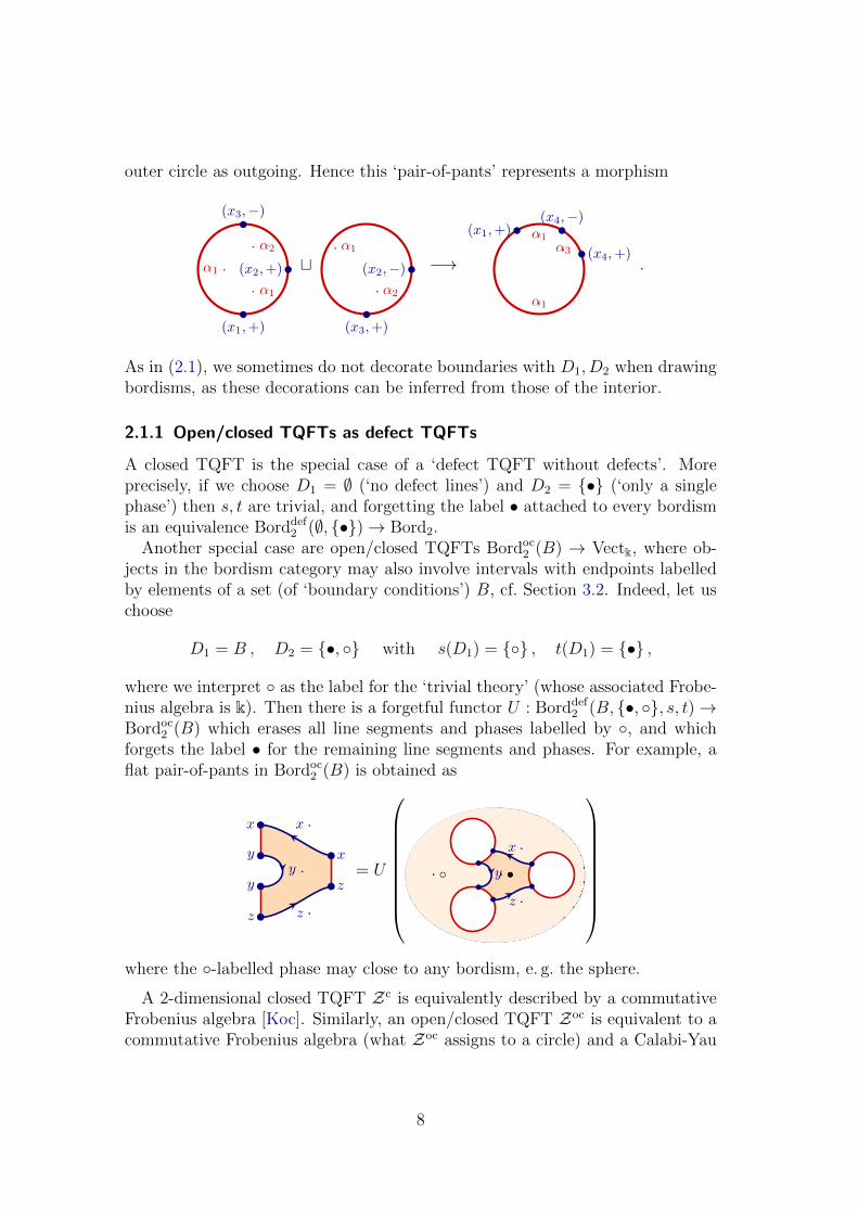
outer circle as outgoing. Hence this ‘pair-of-pants’ represents a morphism
(x3,−)
(x2,+)
(x1,+)
α2
α1
α1 t (x2,−)
(x3,+)
α1
α2
−→
(x1,+)(x4,−)
(x4,+)
α1
α1
α3
.
As in (2.1), we sometimes do not decorate boundaries with D1, D2 when drawingbordisms, as these decorations can be inferred from those of the interior.
2.1.1 Open/closed TQFTs as defect TQFTs
A closed TQFT is the special case of a ‘defect TQFT without defects’. Moreprecisely, if we choose D1 = ∅ (‘no defect lines’) and D2 = • (‘only a singlephase’) then s, t are trivial, and forgetting the label • attached to every bordismis an equivalence Borddef
2 (∅, •)→ Bord2.Another special case are open/closed TQFTs Bordoc
2 (B) → Vectk, where ob-jects in the bordism category may also involve intervals with endpoints labelledby elements of a set (of ‘boundary conditions’) B, cf. Section 3.2. Indeed, let uschoose
D1 = B , D2 = •, with s(D1) = , t(D1) = • ,
where we interpret as the label for the ‘trivial theory’ (whose associated Frobe-nius algebra is k). Then there is a forgetful functor U : Borddef
2 (B, •, , s, t)→Bordoc
2 (B) which erases all line segments and phases labelled by , and whichforgets the label • for the remaining line segments and phases. For example, aflat pair-of-pants in Bordoc
2 (B) is obtained as
x
y
y
z
x
z
x
z
y = U
x
z
y •
where the -labelled phase may close to any bordism, e. g. the sphere.
A 2-dimensional closed TQFT Zc is equivalently described by a commutativeFrobenius algebra [Koc]. Similarly, an open/closed TQFT Zoc is equivalent to acommutative Frobenius algebra (what Zoc assigns to a circle) and a Calabi-Yau
8

category (whose set of objects is B, and whose Hom spaces are what Zoc assigns tointervals), together with certain maps [Laz, AN, MS, LP1]. Below in Section 3.2we will review this in more detail, and in Section 3.3 we will explain how all thesealgebraic structures are naturally obtained from the general perspective of defectTQFT. However, we first need to bring the process
closed
TQFT ≈ Frobenius algebraopen/closed
TQFT ≈ Calabi-Yau categoryadd boundary
structure
to its logical conclusion and show how the expectation
defect
TQFT ≈ pivotal 2-category
can be made rigorous.
2.2 Pivotal 2-categories
We start with a brief review of 2-categories and their graphical calculus; fora more detailed account we refer to [Ben, KS, Lau2]. Let us first recall thatevery k-algebra A can be viewed as the endomorphism space End(∗) of a k-linearcategory with a single object ∗. In this sense a category generalises the idea of‘many algebras together’.
A 2-category is ‘many monoidal categories together’. The precise definition isthat a 2-category is a category enriched over the category of small categories.This means that for any two objects α, β of a 2-category B, there is a categoryB(α, β) whose objects are called 1-morphisms from α to β, and whose morphismsare called 2-morphisms. The composition of two 2-morphisms in B(α, β) is calledvertical composition. Since 1-morphisms can also be composed (being morphismsin B) there are functors
⊗ : B(β, γ)× B(α, β) −→ B(α, γ)
which we refer to as horizontal composition. A good example of a 2-category isthat whose objects, 1- and 2-morphisms are small categories, functors and naturaltransformations, respectively.
The attributes ‘vertical’ and ‘horizontal’ for the two types of composition ina 2-category B derive from the graphical calculus, which allows to perform com-putations in B in terms of so-called string diagrams, according to the followingrules:
• Objects in B label 2-dimensional regions in the plane.
• 1-morphisms X : α → β label smooth lines with α to the right and β tothe left. The lines must be progressive, i. e. at no point on the line may
9

the tangent vector have zero component in upward direction, cf. [BMS,Def. 2.8]. For example:
β α
X
Such an X-line is also identified with the unit 2-morphism 1X ∈ End(X).
• 2-morphisms Φ : X → Y label vertices on a line with label X below andlabel Y above the vertex, respectively:
β α
X
Y
Φ .
This diagram is identified with Φ.
• Vertical composition of Φ : X → Y and Ψ : Y → Z really is vertical, readfrom bottom to top:
X
Y
Z
Φ
Ψ
=
X
Z
ΨΦ .
Note that as above we sometimes suppress labels for 2-dimensional regions.
• Horizontal composition really is horizontal, read from right to left:
γ β α
X
Y
X ′
Y ′
ΦΨ = γ α
X ′ ⊗X
Y ′ ⊗ Y
Ψ⊗ Φ ≡ γ
β
β
α
X
Y
X ′
Y ′
Ψ⊗ Φ
Here we used the additional rule that elements in the set of 2-morphismsHom(X1 ⊗ · · · ⊗ Xm, Y1 ⊗ · · · ⊗ Yn) may be depicted as vertices with mincoming Xi-lines and n outgoing Yj-lines. Consistency with X = X ⊗ 1αthen demands that the unit 1-morphisms 1α can be represented by invisiblelines.
Hence every progressive string diagram represents a 2-morphism by reading it
10

from bottom to top and from right to left. For example
X1 X2 X3 X4
Y1 Y2
Φ1 Φ2
Ψ
= Ψ(Φ1⊗Φ2) : X1⊗X2⊗X3⊗X4 −→ Y1⊗Y2 . (2.2)
But what if the loci of the lines or vertices vary a little? Does
X1 X2 X3 X4
Y1 Y2
Φ1Φ2
Ψ
represent the same 2-morphism as (2.2)? It better should, and this is guaranteedby the following rule:
• String diagrams which are related by progressive isotopies represent thesame 2-morphism [BMS, Sect. 2.2].
This in particular implies the interchange law
(1⊗ Φ) (Ψ⊗ 1) =
Ψ
Φ
=
Ψ
Φ
= (Ψ⊗ 1) (1⊗ Φ) (2.3)
which is a consequence of the functoriality of ⊗.
String diagrams for 2-categories are already reminiscent of local patches on de-fect bordisms. To make this relation precise we need to enlarge the type of stringdiagrams we consider, by giving an orientation to every line, and by allowingthem to make ‘U-turns’. In order to continue to have a 1-to-1 relation betweenisotopy classes of string diagrams and 2-morphisms, we need however to consider2-categories with additional structure: 2-categories ‘with adjoints’.
Given a 1-morphism X : α → β in a 2-category B, we say that X has a leftadjoint if there is †X ∈ B(β, α) together with 2-morphisms
evX : †X ⊗X −→ 1α , coevX : 1β :−→ X ⊗ †X
11

subject to the conditions(1X ⊗ evX
)(
coevX ⊗1X)
= 1X ,(
evX ⊗1†X)(1†X ⊗ coevX
)= 1†X . (2.4)
Since the adjunction maps evX , coevX are something special, they deserve spe-cial diagrammatic notation:
evX =
X†X
, coevX =X †X
. (2.5)
Here we are using our final rule for string diagrams:
• Lines for objects X with an adjoint come with an orientation. Such linesneed not be progressive, but the only non-progressive parts must be dia-grams for adjunction maps as in (2.5) or (2.6). Upward-oriented line seg-ments are labelled X, downward-oriented segments are labelled †X or X†.
In diagrammatic language the conditions (2.4) are easy to remember: they arecalled Zorro moves and state that ‘lines may be straightened out’:
X
X
=
X
X
,
†X
†X
=
†X
†X
.
Similarly, the right adjoint of X ∈ B(α, β) is X† ∈ B(β, α) together withadjunction maps
evX =
X†X
: X ⊗X† −→ 1β , coevX =X† X
: 1α −→ X† ⊗X (2.6)
that satisfy the Zorro moves
X
X
=
X
X
,
X†
X†
=
X†
X†
.
If every 1-morphism in B has a left and a right adjoint, we say that B has adjoints.While it is not difficult to prove that left and right adjoints are unique up to
isomorphism, †X need not be isomorphic to X† in general. However, since fromthe perspective of TQFT taking the adjoint corresponds to orientation reversal
12

on defect lines, we expect †X = X† in the 2-categories we will construct fromdefect TQFTs. More precisely, we will encounter pivotal 2-categories, whichby definition have adjoints with †X = X† for all 1-morphisms X, and whereboth adjoints for 2-morphisms are identified as well. This means we require theidentities
Z†
X†
Φ =
†Z
†X
Φ ,
Y †X†
(Y ⊗X)†
=
†Y†X
†(Y ⊗X)
(2.7)whenever these diagrams make sense.
If the left and right adjoints of a 1-morphism X ∈ B(α, β) coincide, we cancompose coevX with evX , and coevX with evX . These composites are called theleft and right quantum dimensions:
diml(X) =
α
β
X
∈ End(1α) , dimr(X) =
β
α
X
∈ End(1β) .
(2.8)More generally, in a pivotal 2-category the left and right traces of an endomor-phism Ψ ∈ End(X) are defined to be
trl(Ψ) =
αβ
X
Ψ ∈ End(1α) , trr(Ψ) =
βα
X
Ψ ∈ End(1β) . (2.9)
It follows from the first identity in (2.7) that traces have the expected cyclicproperty, i. e. trl(ΦΨ) = trl(ΨΦ) and trr(ΦΨ) = trr(ΨΦ) for any anti-parallel pairof 2-morphisms Φ,Ψ.
The above notions of adjoints, quantum dimensions and traces generalise thecase of finite-dimensional vector spaces V ∈ Vectk. Indeed, †V and V † are givenby the dual vector space V ∗, and evV really is the evaluation V ∗ ⊗k V → k,ϕ ⊗ v 7→ ϕ(v). Choosing a basis ei of V , we set coevV (λ) = λ
∑i ei ⊗ e∗i for
all λ ∈ k, and analogously for evV and coevV . Then one easily verifies the Zorromoves, and (2.9) reduces to the ordinary traces of linear operators (under thecanonical identification V ∗∗ ∼= V ). In particular we have diml(V ) = dimr(V ) =dimk(V ).
13

2.3 Pivotal 2-categories from defect TQFTs
With the above preparations we can now construct, following [DKR], the pivotal2-category BZ associated to a defect TQFT
Z : Borddef2 (D) −→ Vectk
for any set of defect data D = (D1, D2, s, t). It will be convenient to switchbetween source and target maps depending on orientations, for which we define
s(x,+) = s(x) , t(x,+) = t(x) and s(x,−) = t(x) , t(x,−) = s(x)
for all x ∈ D1.Before we start with the construction of BZ , let us lead with its interpretation:
objects = closed TQFTs
1-morphisms = line defects
2-morphisms = ‘local’ operators inserted at defect junctions
vertical composition = operator product (2.10)
horizontal composition = fusion product
unit 1-morphisms = invisible defects
adjunction = orientation reversal
With this in mind it is no surprise that we define the objects of BZ to be thelabel set for 2-dimensional phases on defect bordisms:
Obj(BZ) = D2 .
Later in Section 3.1 we will extract a commutative Frobenius algebra from BZfor every α ∈ D2, so objects really are closed TQFTs.
The set of 1-morphisms α→ β is defined to be((x1, ε1), . . . , (xn, εn)
)∈ (D1 × ±)n
∣∣∣ n > 0 , s(xn, εn) = α , t(x1, ε1) = β ,
s(xi, εi) = t(xi+1, εi+1) for i ∈ 1, 2, . . . , n− 1. (2.11)
Why? Clearly we want a defect line labelled by x ∈ D1 to be a 1-morphismbetween the objects s(x) and t(x):
x
s(x)t(x) . (2.12)
14

But if this defect line is ‘fused’ with another one labelled y ∈ D1 whose sourcecoincides with the target of x,
y
s(y)= t(x)t(y) , (2.13)
there is a priori no element ‘y ⊗ x’ in D1 to label the fusion product of y and x.However, we can compose (2.12) and (2.13) to obtain
xy
s(x)s(y)= t(x)t(y) . (2.14)
This picture should be thought of as the composite 1-morphism of y and x.And in general, any list of composable defect line labels with orientations X =((x1, ε1), . . . , (xn, εn)) as in (2.11) is a 1-morphism from α to β:
xnxn−1xn−2x1
s(xn) = αt(xn)= t(xn−1)s(xn−1)= t(xn−2). . .β = t(x1)
(2.15)
For X = ((x1, ε1), . . . , (xn, εn)) : α→ β and X = ((x1, ε1), . . . , (xm, εm)) : β →γ we define horizontal composition to be concatenation of lists,
X ⊗X =((x1, ε1), . . . , (xm, εm), (x1, ε1), . . . , (xn, εn)
): α −→ γ .
In particular, (2.14) really is the tensor product of (2.12) and (2.13). It is clearthat horizontal composition in BZ is associative, and the unit 1-morphism 1α issimply the empty sequence (n = 0).
The vector space(!) of 2-morphisms Hom(X, Y ) forX = ((x1, ε1), . . . , (xn, εn)) :α→ β and Y = ((y1, ν1), . . . , (ym, νm)) : α→ β is defined to be
Hom(X, Y ) = Z
(y1, ν1)
(y2, ν2)
. . .
(ym−1, νm−1)
(ym, νm)
(x1,−ε1)(x2,−ε2)
. . .
(xn−1,−εn−1)(xn,−εn)
. (2.16)
Why? First we note that it is only at this point that we make use of the functor Z.(Objects and 1-morphisms in BZ are built only from the defect data D1, D2, s, t.)
15

Secondly, according to our interpretation (2.10), 2-morphisms should correspondto junction points such as
αβ
x1 x2 xn
y1 y2 ym. . .
. . .
, (2.17)
but we were not provided with a set D0 to label such points. However, we canuse Z to build such a set; in fact it is precisely given by (2.16)! To see this, wecut a little hole around the vertex in (2.17) and keep track of orientations byassigning + to intersection points of lines pointing away from the hole, and − tothose pointing in the opposite direction:
x1 x2 xn
y1 y2 ym. . .
. . .
− − +
− + −
αβ
Note that we have not lost any information. But now the boundary of the holeis an object in Borddef
2 (D). Applying Z as in (2.16) to it produces the label setfor vertices allowed by the TQFT.
Next we define vertical composition in BZ . As in the familiar case of closedTQFT, this product is obtained by applying Z to a pair-of-pants. In detail, letus consider a 2-morphism Φ ∈ Hom(X, Y ) as above, and another 2-morphism
16

Ψ ∈ Hom(Y, Z) where Z = ((z1, µ1), . . . , (zk, µk)) : α→ β. Then we define
Ψ Φ = Z
(z1, µ1)
(z2, µ2)
(zk, µk)
(x1,−ε1)
(x2,−ε2)
(xn,−εn)
(z1, µ1) (zk, µk)
(y1,−ν1) (ym,−νm)
(y1, ν1) (ym, νm)
(x1,−ε1) (xn,−εn)
αβ
. . .
. . .
. . .
(Ψ⊗k Φ
)∈ Hom(X,Z)
where the two inner boundary circles are incoming, and the outer circle is out-going, and the orientations of defect lines can be inferred from those of theirendpoints. Functoriality of Z implies that this composition is associative, and itis unital with respect to the identity
1X = Z
(x1, ε1)
(x2, ε2)
(xn, εn)
(x1,−ε1)(x2,−ε2)
(xn,−εn)
αβ . . .
(1) .
Here the disc is viewed as a bordism from the empty set to the boundary circle,so applying Z gives a linear map k→ End(X).
To complete the construction of BZ as a 2-category, we need to define horizontalcomposition of 2-morphisms. Again this involves a pair-of-pants, but this timethe defect decoration is different: for Φ ∈ Hom(X, Y ) and Φ ∈ Hom(X, Y ) where
17

X, Y : α→ β and X, Y : β → γ, we set
Φ⊗ Φ = Z
(y1, ν1)
(y2, ν2)
(ym, νm) (y1, ν1)
(y2, ν2)
(ym, νm)
(x1, ε1)
(x2, ε2)
(xn, εn) (x1, ε1)
(x2, ε2)
(xn, εn)
αβγ
. . .
. . . . . .
. . .
(Φ⊗k Φ
).
It remains to give BZ adjoints and show that it is pivotal. Since adjointscorrespond to orientation reversal, adjoints are defined to have opposite signs εand reversed order:
BZ(α, β) 3 X =((x1, ε1), . . . , (xn, εn)
)=⇒ †X ≡ X† =
((xn,−εn), . . . , (x1,−ε1)
)∈ BZ(β, α) .
Note that this was already implicitly used in the definition (2.16), so we haveHom(X, Y ) = Hom(1β, Y ⊗X†).
To exhibit †X as the left adjoint to X we define the adjunction maps
evX =
X†X
= Z
(x1, ε1) (x1,−ε1)
(x2, ε2) (x2,−ε2)
(xn, εn) (xn,−εn)
α
β
...
(1) : †X ⊗X −→ 1α (2.18)
and
coevX =X †X
= Z
(xn,−εn)(xn, εn)
(x2,−ε2)(x2, ε2)(x1,−ε1)(x1, ε1)
β
α...
(1) : 1β −→ X⊗†X . (2.19)
18

The maps evX , coevX exhibiting X† as a right adjoint are defined analogously,by reversing all orientations and orders in (2.18) and (2.19). Proving that theZorro moves hold is straighforward, for example
X
X
= Z
β α
X
X
†X
(coevX ⊗k evX)
= Z
β α
X
X
†X
(1)
= Z
αβ
X
(1) =
X
X
,
where in the second step we used functoriality of Z, and in the third step weused isotopy invariance in Borddef
2 (D). The pivotality conditions (2.7) are provedsimilarly, and we have arrived at the following result:
19

Theorem 2.1. Every 2-dimensional defect TQFT Z gives rise to a k-linear piv-otal 2-category BZ as constructed above.
By construction, string diagrams in BZ are correlators of Z. More precisely,a priori the 2-morphisms in BZ only capture the action of Z on defect bordismsthat can be embedded into the plane. But what about the other bordisms forwhich this in not possible, such as the sphere S2? Below in Section 3.1 wewill see how sphere correlators can be evaluated in BZ – under one additionalassumption. Namely, in order to get from arbitrary defect bordisms Σ to stringdiagrams, one can project Σ onto a fixed plane, and generically this leads to astring diagram.3 If this projection is not injective, then patches of different phasesof Σ will overlap on the plane. Hence one is led to a multiplicative structureon the set D2 labelling phases, i. e. the objects of BZ . More precisely, for thegeneral procedure to consistently express defect correlators as string diagrams inBZ , i. e. to produce the same result for every generic projection, BZ should bemonoidal. This is in fact true of all the examples associated to defect TQFTsI know of, and it is natural to conjecture that 2-dimensional defect TQFTs areequivalent to k-linear monoidal pivotal 2-categories.
It is still an open problem to classify defect TQFTs, by proving a theoremalong the lines of the above conjecture. Thus the situation is different from thatof closed TQFTs (which are equivalent to commutative Frobenius algebras), andthat of open/closed TQFTs. The latter are basically equivalent to Calabi-Yaucategories and the ‘Cardy condition’, the details of which we review in Section 3.2.
Before moving on to examples, we mention that the classification question isalready settled for another, related type of ‘enhanced’ TQFTs. This howevercomes at the price of defining such TQFTs as higher functors between highercategories, contrary to the approach discussed above where a higher category isconstructed from an ordinary functor. Indeed, a 2-1-0-extended TQFT is a sym-metric monoidal 2-functor Bord2,1,0 → Algk, where roughly Bord2,1,0 has points,lines, and 2-manifolds with corners (all oriented) as objects, 1-, and 2-morphisms,respectively, while Algk consists of finite-dimensional k-algebras, bimodules, andbimodule maps. It was shown in [SP] that such extended oriented TQFTs areequivalent to separable symmetric Frobenius algebras in Algk. This is preciselyas predicted by the cobordism hypothesis, as homotopy fixed points of the trivialSO(2)-action on fully dualisable objects in Algk are separable symmetric Frobe-nius algebras [HSV].
2.4 Examples
In this section we sketch a number of pivotal 2-categories which are known (thosein Sections 2.4.1, 2.4.7, and 2.4.8) or believed (those in Sections 2.4.2–2.4.6) to
3The situation here is similar to that of knots in R3 and their knot diagrams.
20

arise from defect TQFTs as described above. Presenting all details and thenecessary background would inflate the length of the exposition exponentially.Hence we content ourselves with a rough account which mainly aims to subsumeall examples under the common heading of defect TQFT, and to showcase thebroad spectrum of interesting pivotal 2-categories.
In fact most of the examples are not strict 2-categories, but their weak cousinscalled bicategories for which horizontal composition is associative and unital onlyup to coherent isomorphisms [Ben]. Luckily, every (pivotal) bicategory is equiva-lent to a (pivotal) 2-category,4 so we just as well may work with the bicategoriesthat ‘occur in nature’.
2.4.1 State sum models
Separable symmetric Frobenius k-algebras also appear as special cases in defectTQFT. Indeed, they are the objects of a bicategory ssFrobk, whose 1-morphismsfrom A to B are finite-dimensional B-A-bimodules, and 2-morphisms are bimod-ule maps. Horizontal composition of M : A → B and N : B → C is thetensor product N ⊗BM over the intermediate algebra, and the unit 1-morphism1A is A viewed as a bimodule over itself.5 The left and right adjoints of a 1-morphism M are given by the dual bimodule M∗. Thanks to the natural isomor-phism M∗∗ ∼= M , the k-linear bicategory ssFrobk is also pivotal.
It was shown in [DKR, Sect. 3] that ssFrobk is equivalent to the 2-category BZss
associated to a special defect TQFT Zss. To wit,
Zss : Borddef2
(Dss
1 , Dss2 , s, t
)−→ Vectk
is a state sum model, generalising the state sum constructions of closed [FHK] andopen/closed [LP2] 2-dimensional TQFTs. Here the defect data consist of the setDss
2 of separable symmetric Frobenius algebras, the set Dss1 of B-A-bimodules M
for all A,B ∈ Dss2 , and we have s(M) = A and t(M) = B.
As in the closed and open/closed case, the construction of Zss involves a choiceof triangulation for objects and bordisms in Borddef
2 (Dss), a decoration of everytriangulation with algebraic data, and a projection procedure that ensures thatthe construction is independent of the choice of triangulation. In the case of Zss,additional technicalities arise from the compatibility of triangulation and defectlines. We refer to [DKR] for all details and only note that on objects, Zss is
4An analogous maximal ‘strictification’ result does not hold for tricategories, which explainspart of the richness of 3-dimensional TQFT.
5It follows that invertible 1-morphisms in ssFrobk are precisely Morita equivalences.
21

defined by
Zss
(Mn, εn)(Mn−1, εn−1)
(M1, ε1)
...
(M2, ε2)A1
An−1
An
= An
(M εn
n ⊗An−1 Mεn−1
n−1 ⊗An−2 · · · ⊗A1 Mε11
)
where M+ = M and M− = M∗, and for an A-A-bimodule M , the vector spaceAM is defined to be the cokernel of the map A⊗M →M , a⊗m 7→ am−ma.It follows that Zss( A ) = A/[A,A] is the 0-th Hochschild homology.
Finally we note that ssFrobk naturally has a monoidal structure, given bytensoring over the field k. The trivial Frobenius algebra k is the unit object.Invertible objects are those algebras A ∈ ssFrobk for which there exist algebrasB,B′ ∈ ssFrobk such that A ⊗k B and B′ ⊗k A are Morita equivalent to k. Itfollows that isomorphism classes of invertible objects in ssFrobk precisely formthe Brauer group of k.
2.4.2 Algebraic geometry
Next we consider a more geometric example, the bicategory Var. It has smoothand proper varieties as objects, 1-morphisms are Fourier-Mukai kernels, and 2-morphisms are their maps up to quasi-isomorphism. Hence for U, V ∈ Var, wehave that
Var(U, V ) = Db(coh(U × V )) =: D(U × V )
is the bounded derived category of coherent sheaves on the product space. Hor-izontal composition of kernels E ,F is the convolution E F , and the unit 1U isthe structure sheaf O∆U
of the diagonal ∆U ⊂ U × U .Adjunctions in Var were studied in detail in [CW]. The ‘naive’ adjoint ofE ∈ Var(U, V ) is E∨ := HomD(U×V )(E , U × V ), but by Grothendieck duality thetrue adjoints are obtained by ‘twisting with the Serre kernel’: we have
†E = E∨ ΣV , E† = ΣU E∨ ,
where ΣU is obtained from the canonical line bundle ωU as ΣU = (∆U)∗ωU [dimU ].It follows that Var is not pivotal ‘on the nose’, but only has polite dualities asexplained in [CW].
One way to look at the failure of Var being strictly pivotal is via its interpre-tation in terms of B-twisted sigma models, whose defects were also studied in[Sar, AS]. Indeed, in theoretical physics to every object U in Var one associatesa field theory called an ‘N = (2, 2) supersymmetric sigma model’. There is aprocedure called ‘topological B-twist’ [HKK+, Ch. 16] that produces a closed 2-dimensional TQFT from U if it is a Calabi-Yau variety, i. e. ωU is trivial. Indeed,
22
in this case Hochschild homology and cohomology coincide up to shift and areisomorphic to Dolbeault cohomology H∂(U). Then together with the Mukai pair-ing H∂(U) is a commutative Frobenius algebra in the category of graded vectorspaces Vectgr
C . Hence H∂(U) describes a closed TQFT Bord2 → VectgrC . The fact
that H∂(U) is only graded commutative can be traced back to the supersymmetryof the original sigma model.
To Var one can associate the defect data DB given by DB2 = Obj(Var), DB
1 =Obj(Var(U, V ))U,V ∈DB
2and obvious source and target maps. Then it is natural
to conjecture that there is a defect TQFT ZB : Borddef2 (DB) → Vectgr
C whoseassociated 2-category BZB is equivalent to Var. Furthermore, taking products ofvarieties gives Var a monoidal structure.
2.4.3 Symplectic geometry
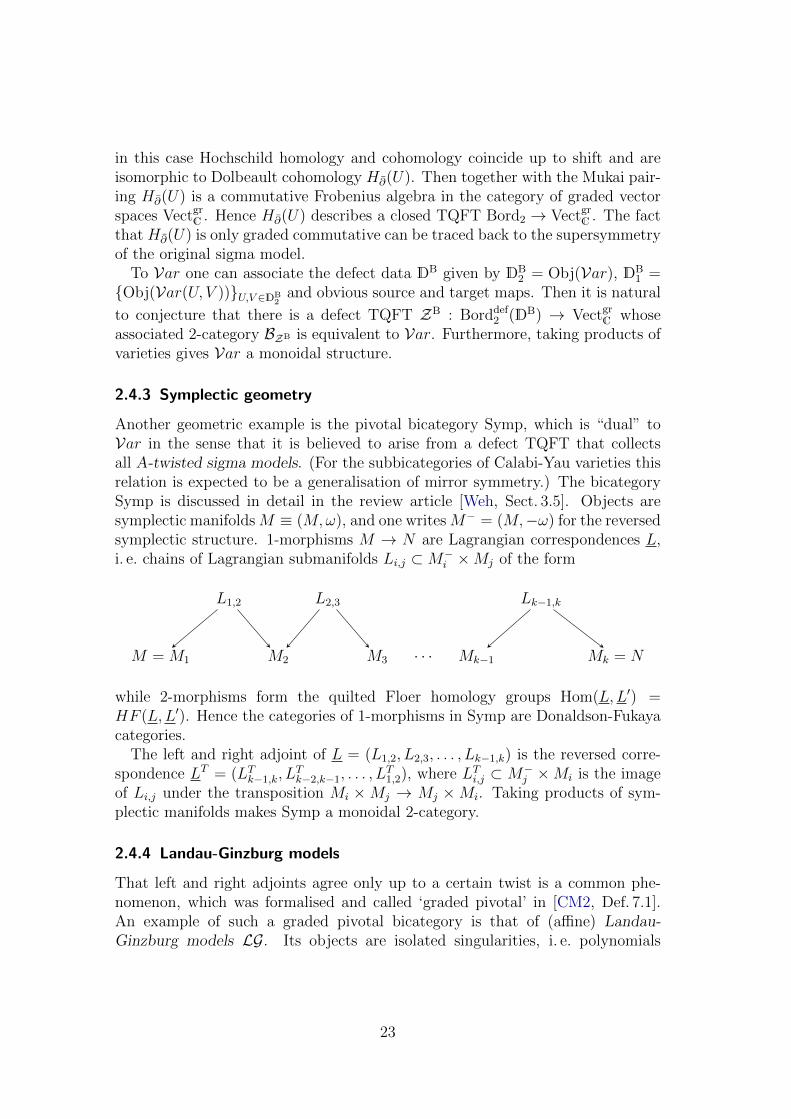
Another geometric example is the pivotal bicategory Symp, which is “dual” toVar in the sense that it is believed to arise from a defect TQFT that collectsall A-twisted sigma models. (For the subbicategories of Calabi-Yau varieties thisrelation is expected to be a generalisation of mirror symmetry.) The bicategorySymp is discussed in detail in the review article [Weh, Sect. 3.5]. Objects aresymplectic manifoldsM ≡ (M,ω), and one writesM− = (M,−ω) for the reversedsymplectic structure. 1-morphisms M → N are Lagrangian correspondences L,i. e. chains of Lagrangian submanifolds Li,j ⊂M−
i ×Mj of the form
L1,2 L2,3 Lk−1,k
M = M1 M2 M3 · · · Mk−1 Mk = N
while 2-morphisms form the quilted Floer homology groups Hom(L,L′) =HF (L,L′). Hence the categories of 1-morphisms in Symp are Donaldson-Fukayacategories.
The left and right adjoint of L = (L1,2, L2,3, . . . , Lk−1,k) is the reversed corre-spondence LT = (LTk−1,k, L
Tk−2,k−1, . . . , L
T1,2), where LTi,j ⊂ M−
j ×Mi is the imageof Li,j under the transposition Mi ×Mj → Mj ×Mi. Taking products of sym-plectic manifolds makes Symp a monoidal 2-category.
2.4.4 Landau-Ginzburg models
That left and right adjoints agree only up to a certain twist is a common phe-nomenon, which was formalised and called ‘graded pivotal’ in [CM2, Def. 7.1].An example of such a graded pivotal bicategory is that of (affine) Landau-Ginzburg models LG. Its objects are isolated singularities, i. e. polynomials
23

W ∈ C[x1, . . . , xn] for some n ∈ N such that the Jacobi ring
JacW := C[x1, . . . , xn]/(∂x1W, . . . , ∂xnW )
is finite-dimensional over C.6 A 1-morphism from W ∈ C[x1, . . . , xn] ≡ C[x] toV ∈ C[z1, . . . , zm] ≡ C[z] is a matrix factorisation X of V − W . This meansthat X is a free finite-rank Z2-graded C[z, x]-module X = X0⊕X1 together withan odd map dX ∈ End1
C[z,x](X) such that d2X = (V −W ) · 1X . A 2-morphism
between X, Y ∈ LG(W,V ) is an even C[z, x]-linear map Φ : X → Y up tohomotopy with respect to the twisted differentials dX and dY . If one choosesbases of X and Y , then dX , dY and Φ are represented by odd and even matrices,respectively.
Horizontal composition in LG is given by tensoring over the intermediatepolynomial ring.7 The unit 1W is a deformation of the Koszul complex of(∂x1W, . . . , ∂xnW ), which in the simplest case of W = xd means that d1W
is represented by the matrix ( 0 x−x′(xd−x′d)/(x−x′) 0 ). In general one finds that
End(1W ) ∼= JacW .Not only horizontal composition, but also adjunctions in LG are under very
good control. Up to a shift, †X and X† are simply given by HomC[z,x](X,C[z, x]),but also the adjunction maps evX , coevX etc. were computed explicitly in termsof Atiyah classes in [CM2]. In this way we could show that LG is graded piv-otal. Furthermore, one obtains neat formulas for quantum dimension and traces(recall (2.8) and (2.9)), for example
dimr(X) = (−1)(m+1
2 ) ResC[x,z]/C[z]
[str(∂x1dX . . . ∂xndX ∂z1dX . . . ∂zmdX
)dx
∂x1W . . . ∂xnW
]
where X ∈ LG(W,V ) is as above.Using the construction of [Shu] one may verify that LG is a monoidal bicategory,
where the tensor product of W ∈ C[x] with V ∈ C[z] is W + V ∈ C[z, x], and0 ∈ C is the monoidal unit. It is expected (but not proven) that there exists adefect TQFT ZLG : Borddef
2 (DLG) → VectZ2k such that LGk is equivalent to the
2-category BZLG associated to ZLG.
2.4.5 Differential graded categories
Twisted sigma models and Landau-Ginzburg models fit into a larger framework ofdifferential graded (dg) categories [Toe]. Indeed, there is a bicategoryDGsat
k whoseobjects are ‘saturated’ dg categories, and whose 1- and 2-morphisms are certain
6In fact there is a graded pivotal bicategory LGk for any commutative ring k as explained in[CM2], but the finiteness condition on its objects is more involved for k 6= C.
7This can be algorithmically computed by splitting an idempotent [DM], which was used in[CM1] to compute the homological knot invariants of Khovanov and Rozansky [KR].
24
resolutions of dg functors and natural transformations, respectively. Every objectU ∈ Var, M ∈ Symp, or W ∈ LG can be viewed as an object in DGsat
k by takingthe unique dg enhancemens of D(U), Symp(pt,M), or LG(0,W ), respectively.Then the bicategories Var, Symp and LG are quasi-equivalent to the (distinct)corresponding full subbicategories of DGsat
k . More generally, one might think ofDGsat
k as the bicategory of TQFTs arising from topologically twisting N = (2, 2)supersymmetric quantum field theories.
Working in the enlarged framework of DGsatk also has the advantage of com-
paring sigma models and Landau-Ginzburg models in a more natural context. Inparticular, homological mirror symmetry is a statement internal to DGsat
k , andit is tempting to speculate that there is a truly 2-categorical generalisation ofmirror symmetry, taking place in a suitable enlargement of DGsat
k .8
As shown in [BFK, App. A.2], DGsatk is equivalent to the more manageable
bicategory DGspk of smooth and proper dg algebras. The 1-morphisms M : A→ B
in DGspk are perfect dg (Aop⊗kB)-bimodules, i. e. HomD(Aop⊗kB)(M,−) commutes
with arbitrary coproducts, and 2-morphisms are maps of dg bimodules up toquasi-isomorphisms. Horizontal composition is the left-derived tensor productover the intermediate algebra. It follows from the discussion in [BFK] that DGsp
kis graded pivotal, and analogously to the situation in Sections 2.4.2 and 2.4.4,adjoints are given by the naive dual together with a twist by Serre functors.
Tensoring over the field k gives the bicategories DGsatk and DGsp
k a naturalmonoidal structure [Toe].
2.4.6 Categorified quantum groups
Pivotal 2-categories also feature prominently in higher representation theory (seee. g. [Lau2, Sect. 1] for a gentle introduction), which in turn plays a unifying rolein the theory of homological link invariants. A key idea behind ‘2-Kac-Moodyalgebras’ [Rou] and ‘categorified quantum groups’ [Lau1, KL] is to representthem not on vector spaces, but on linear categories. This leads one to replacethe (quantum) Serre relations, which are equalities between expressions involvingthe generators Ei, Fj, by natural transformations ηk between the correspondingexpressions of functors Ei,Fj. This theory is considerably richer than its classicalcounterpart, partly because of nontrivial relations which have to be imposed onthe ηk.
Associated to any Kac-Moody algebra g there is a k-linear pivotal 2-categoryUQ(g). The precise definition fills several pages (cf. the above references), buthere is a sketch: First one picks a ‘Cartan datum and choice of scalars Q’; thisin particular gives a weight lattice X with simple roots αi, and a symmetrisablegeneralised Cartan matrix. Objects of UQ(g) are simply weights λ ∈ X, and
8The process of orbifold completion discussed in Section 2.4.8 below may play a role here.
25

1-morphisms are formal polynomials in expressions of the form
1λ , 1λ+αiEi = 1λ+αiEi1λ = Ei1λ , 1λ−αiFi = 1λ−αiFi1λ = Fi1λ .
2-morphisms are k-spans of compositions of certain string diagrams which encodethe categorification of the Serre relations for g, subject to a list of relations. Theserelations in particular describe biadjunctions (again up to shifts) between Ei1λand Fi1λ. As explained in [BHLW], the parameters Q can be chosen such thatthese adjunctions become a strictly pivotal structure on UQ(g). It is an openproblem to determine whether there is a natural monoidal structure on UQ(g).
2.4.7 Surface defects in 3-dimensional TQFT
One generally expects n-dimensional TQFTs to appear as defects of codimen-sion 1 in (n+ 1)-dimensional TQFTs. At least for n = 2 this is a rigorous resultalso from the algebraic perspective: In [CMS] we introduced 3-dimensional defectTQFTs Z, from which we went on to construct a certain type of 3-category TZ .More precisely, TZ is a k-linear ‘Gray category with duals’ – categorifying theconstruction of Section 2.3. This implies in particular that TZ(u, v) is a k-linearpivotal 2-category for all u, v ∈ TZ . And since the objects (interpreted as ‘sur-face defects’) of TZ(u, v) are the 1-morphisms of a 3-category, TZ(u, v) is monoidalwhenever u = v.
2.4.8 Orbifold completion
As a final source of pivotal 2-categories we point to the procedure of ‘orbifoldcompletion’ of [CR]. Inspired by the orbifold construction from finite groupactions and their generalisation in rational conformal field theory [FFRS], orbifoldcompletion takes a pivotal bicategory B as input and produces a new pivotalbicategory Borb, into which B fully embeds. It is a completion because there isan equivalence (Borb)orb
∼= Borb.Objects of Borb are pairs (α,A) where α ∈ B and A is a separable symmetric
Frobenius algebra – not necessarily in Vectk, but in the category B(α, α). A1-morphism (α,A) → (β,B) in Borb is a 1-morphism X ∈ B(α, β) togetherwith the structure of a B-A-bimodule, and 2-morphisms are those in B whichare also bimodule maps. Horizontal composition is the tensor product over theintermediate algebra, and 1(α,A) = A viewed as an A-A-bimodule.
The simplest case of orbifold completion reproduces state sum models. Hereas the input bicategory B one takes the ‘trivial’ bicategory BVectk which has asingle object with Vectk as its endomorphism category. Then by constructionand in the notation of Section 2.4.1 we have
ssFrobk ∼= (BVectk)orb .
26

Examples of separable Frobenius algebras which do not live in Vectk are pro-vided by group actions. For a finite group G and some pivotal bicategory B, letDg ∈ B(α, α) for all g ∈ G such that Dg ⊗Dh
∼= Dgh coherently, and let B(α, α)have finite sums. Then there are as many inequivalent separable Frobenius alge-bras structures on AG :=
⊕g∈GDg as there are elements in H2(G,k×) [BCP2],
and AG is symmetric if its Nakayama automorphism is the identity. Interestingly,not all separable Frobenius algebras come from group actions, cf. [CRCR].
The adjoint of X ∈ Borb((α,A), (β,B)) is †X = X† ∈ B(β, α) together with theadjunction maps
evX =
A
X†X
ξ , coevX = ϑ
B
X †X
where ξ : †X ⊗B X → †X ⊗ X and ϑ : X ⊗ †X → X ⊗A †X are the splittingand projection maps (which we require to exist, cf. [CR, Lem. 2.3]). In fact, thiscontinues to hold if A and B are not required to be symmetric, but then theiractions on †X and X† are twisted by Nakayama automorphisms as explained in[CR, Sec. 4.3], generalising the situation with Serre functors in Sections 2.4.2,2.4.4 and 2.4.5, see [BCP1, CQV].
If B is monoidal then Borb is expected to be monoidal as well. One may eitherargue along the lines of [Shu], or via a universal property for the operation (−)orb.
3 Open/closed TQFTs from pivotal 2-categories
In Section 2.1.1 we easily obtained closed and open/closed TQFTs from defectTQFTs, simply by forgetting part of the structure of the defect bordism categoryBorddef
2 (D). In the present section we elucidate this relation by constructing anopen/closed TQFT from any object in a k-linear pivotal bicategory (satisfyingtwo natural assumptions). We treat the purely closed case in Section 3.1, and thefully open/closed case in Section 3.3. The algebraic description of open/closedTQFTs in terms of Calabi-Yau categories is reviewed in Section 3.2.
3.1 Closed TQFTs from pivotal 2-categories
For completeness, we briefly recall how closed TQFTs Zc : Bord2 → Vectk areequivalent to commutative Frobenius algebras in Vectk. By a classical result[Koc], the bordism category Bord2 is generated by
, , , , (3.1)
27

where from now on incoming/outgoing boundaries are placed at the bottom/topof pictures of bordisms. The relations between the generators (3.1) precisely saythat the vector space Zc(S1) together with multiplication Zc( ), unit Zc( )(1)
and pairing Zc( ) Zc( ) is a commutative Frobenius algebra.Given a k-linear pivotal bicategory B, we would now like to construct a com-
mutative Frobenius algebra Aα naturally associated to every object α ∈ B. Ourinterpretation (2.10) of such bicategories in the context of defect TQFT suggeststhat the underlying vector space of Aα should be the space of endomorphisms ofthe unit 1α:
Aα = End(1α) .
Indeed, we interpret 1α as the invisible defect, and elements φ ∈ End(1α) corre-spond to operators living on an invisible line with no further ‘defect conditions’:
α
φ ∈ End(1α) .
Hence in standard jargon, φ is a field ‘inserted in the bulk’ of the ‘theory’ α.As the 2-endomorphism space in a k-linear bicategory, Aα is manifestly an
associative unital k-algebra. Furthermore, using the interchange law (2.3) onecan show that in any monoidal category the endomorphisms of the unit form acommutative monoid [EGNO, Prop. 2.2.10].
It remains to endow Aα with a nondegenerate pairing which is compatible withmultiplication. There are various ways to ensure the existence of such a pairing.We will see how it follows from
Assumption 3.1. The k-linear pivotal bicategory B is monoidal9 with dualssuch that B(O,O) ∼= Vectk, where O ∈ B is the unit object.
We observe that all our examples in Section 2.4 are known or expected tosatisfy this condition. Further we recall that as noted after Theorem 2.1 it isnatural to expect the bicategories arising from defect TQFTs to come with amonoidal structure: for α, β ∈ B their tensor product α β corresponds to the‘tensor product theory’ attached to the fusion of two bordism patches labelled αand β. The unit O ∈ B corresponds to the ‘trivial theory’. This is consistentwith AO = End(1O) ∼= k being the trivial commutative Frobenius algebras inVectk ∼= B(O,O). Finally, the dual α# of an object α ∈ B is interpreted as alabel for a bordism patch with opposite orientation.
9Monoidal bicategories are defined for example in [SP] or [Shu]. By a ‘monoidal bicategorywith duals’ we mean a ‘Gray category with duals and only a single object’ as defined e. g. in[BMS, Sect. 3.3] or [CMS, Sect. 3.2.2].
28

How can we endow Aα = End(1α) with a nondegenerate pairing using Assump-tion 3.1? Recall that the pairing of the Frobenius algebra associated to a closedTQFT Zc is the ‘sphere correlator’
Zc( )
Zc
( )= Zc
( ): Zc(S1)⊗k Zc(S1) −→ k .
From a bicategory B as in Assumption 3.1 we can build such pairings by mim-icking the above construction as follows. We consider a sphere S2 labelled byα ∈ B. Then we project the sphere onto some plane, producing a disc:
α −→ α α#
The disc is labelled by the product α α# because the rear part of the spherehas opposite orientation with respect to the plane.
We now interpret the disc as a string diagram in B! The preimage of the disc’sboundary is simply the great circle on the sphere which is parallel to the chosenprojection plane. Since any plane will do, this great circle is nothing special –in fact it is invisible on the sphere. Hence we label it with the ‘invisible defect’1α ∈ B(α, α).
Labelling the inside and outside of the sphere with the trivial object O, theboundary of the disc is labelled by the 1-morphism
1α ∈ B(O, α α#
)corresponding to 1α under duality in B. So finally the ‘sphere correlator’ forAα = End(1α) is defined to be
⟨−,−
⟩α
: Aα⊗kAα −→ k , φ1⊗φ2 7−→ α α#
1α
φ1φ2 ∈ End(1O) ∼= k (3.2)
where the string diagram represents the map ev1α (11α
⊗ φ1φ2) coev1α: k→ k,
i. e. the trace trl(φ1φ2). Thus the pairing 〈−,−〉α is manifestly compatible withmultiplication, and it follows from Theorem 3.6 below that 〈−,−〉α is nondegen-erate. Hence we have arrived at a closed TQFT:
Theorem 3.2. Let B be a bicategory satisfying Assumption 3.1. Then for everyα ∈ B, the vector space End(1α) naturally has the structure of a commutativeFrobenius algebra.
29

3.2 Open/closed TQFTs and Calabi-Yau categories
An open/closed TQFT [Laz, MS, LP1] is a symmetric monoidal functor
Zoc : Bordoc2 (B) −→ Vectk (3.3)
where B is some set, whose elements are referred to as boundary conditions. Theobjects of the bordism category Bordoc
2 (B) are disjoint unions of circles S1 andunit intervals Iab whose endpoints are labelled by a, b ∈ B:
Iab =b a
.
Morphisms in Bordoc2 (B) are bordism classes generated by the list (3.1) together
with the classes of the following decorated manifolds with corners for all a, b, c, d ∈B:
c b b a
ac
,
cbba
a c
,a a
,aa,
a b c d
c d a b
,
a a
,
aa
(3.4)
subject to the relations (3.5)–(3.12) below as well as the relations for which
state that together with the twist , the category Bordoc2 (B) has a symmetric
monoidal structure. It follows that Bord2 is a non-full subcategory of Bordoc2 (B).
The relations on the generators (3.4) are the intuitively clear equalities
= , = , (3.5)
= = , = = , (3.6)
= = , (3.7)
= , (3.8)
30
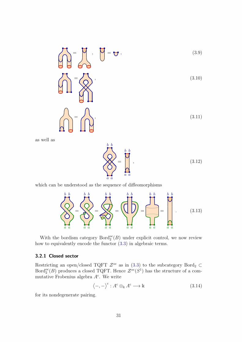
= , = , (3.9)
= , (3.10)
= , (3.11)
as well asbb
aa
=
b b
a a
, (3.12)
which can be understood as the sequence of diffeomorphisms
bb
aa
=
bb
aa
=
a a
b b
=
bb
aa
=
bb
aa
=
b b
a a
. (3.13)
With the bordism category Bordoc2 (B) under explicit control, we now review
how to equivalently encode the functor (3.3) in algebraic terms.
3.2.1 Closed sector
Restricting an open/closed TQFT Zoc as in (3.3) to the subcategory Bord2 ⊂Bordoc
2 (B) produces a closed TQFT. Hence Zoc(S1) has the structure of a com-mutative Frobenius algebra Ac. We write⟨
−,−⟩c
: Ac ⊗k Ac −→ k (3.14)
for its nondegenerate pairing.
31

3.2.2 Open sector
Let Bordo2(B) be the subcategory of Bordoc
2 (B) whose objects are only labelledintervals (and no circles), and whose morphisms are generated by the first fivebordisms in (3.4), subject to (3.5)–(3.8) and the twist relations. By definition anopen TQFT is a symmetric monoidal functor Bordo
2(B)→ Vectk.We construct a category Co from Zoc restricted to Bordo
2(B) as follows. Theset of objects is the set of boundary conditions,
Obj(Co) = B ,
and Hom spaces are what Zoc assigns to labelled intervals,
Hom(a, b) = Zoc(b a
).
Composition is defined to be
Zoc
(c b b a
ac ): Hom(b, c)× Hom(a, b) −→ Hom(a, c) .
It is associative by relation (3.5) and unital thanks to (3.6). This establishes thatCo is a k-linear category.
The relations (3.7) and (3.8) endow Co with additional structure. For all a, b ∈B there are k-linear pairings
⟨−,−
⟩ab
= Zoc
(a b b a
): Hom(b, a)⊗k Hom(a, b) −→ k . (3.15)
By relation (3.8) these pairings are symmetric in the sense that 〈Φ,Ψ〉ab =〈Ψ,Φ〉ba, and they are nondegenerate since
=
according to (3.6) and (3.7). Finally, the pairings are compatible with multipli-cation, 〈Φ1,Φ2Φ3〉ab = 〈Φ1Φ2,Φ3〉ac, by definition of the pairing and associativ-ity (3.5).
It follows from the above that the vector spaces End(a) have the structureof a symmetric Frobenius algebra. Hence one can think of Co as ‘many Frobe-nius algebras glued together’. Unfortunately, the name ‘Frobenius category’ wasalready taken,10 and instead the term ‘Calabi-Yau’ category is used.
10A Frobenius category is a Quillen exact category with enough injectives and enough projec-tives, such that injectives and projectives coincide.
32

To give the definition we first broaden the context. A Serre functor on ak-linear category C is a functor Σ : C → C together with isomorphisms
ηab : Hom(a, b) ∼=−→ Hom
(b,Σ(a)
)∗which are natural in a, b ∈ C. From this one obtains the nondegenerate Serrepairings⟨
−,−⟩ab
: Hom(b,Σ(a)
)⊗k Hom
(a, b)−→ k , Ψ⊗ Φ 7−→ ηaa(1a)(ΨΦ)
by duality. By definition a Calabi-Yau category is a k-linear category C togetherwith a trivial Serre functor Σ = 1C. (If C is a triangulated category, then theSerre functor may be the identity only up to a shift.)
The eponymous example of a (triangulated) Calabi-Yau category is thebounded derived category of coherent sheaves on a Calabi-Yau variety. Indeed,as was noted in Section 2.4.2, the Serre functor on Db(coh(U)) for any smoothand proper variety U is ΣU
∼= ωU [dimC U ] ⊗C (−). But U is Calabi-Yau iff thecanonical line bundle ωU is trivial. In light of the results of Section 3.3 below,Section 2.4 provides many further examples of Calabi-Yau categories.
It follows that the category Co we constructed from the open TQFT Zoc|Bordo2(B)
is Calabi-Yau with Serre pairings (3.15). It was shown in [Laz, MS, LP1] thatthe converse is also true:
Theorem 3.3. The above construction is an equivalence of groupoids betweenopen TQFTs and Calabi-Yau categories.
3.2.3 Open/closed sector
It remains to work out the algebraic meaning of the last two generators in (3.4)as well as their relations (3.9)–(3.12). For this, we first define the bulk-boundarymaps to be
βa := Zoc
( a a ): Ac −→ End(a)
for all a ∈ B. It maps the closed sector (or ‘bulk theory’) to the open sector(with ‘boundary condition’ a).
Due to relations (3.9) and (3.10), βa is a map of algebras into the centre ofEnd(a), i. e.
βa(φ) Ψ = Ψ βa(φ)
for all φ ∈ Ac and Ψ ∈ End(a). Furthermore, the boundary-bulk map (whichneed not be a map of algebras)
βa := Zoc
(aa
): End(a) −→ Ac
33

is adjoint to βa with respect to the Frobenius pairings by (3.11):⟨βa(Ψ), φ
⟩c
=⟨
Ψ, βa(φ)⟩aa.
The most interesting condition on the maps βa derives from (3.12). For Φ ∈End(a) and Ψ ∈ End(b) let us consider the map
ΨmΦ : Hom(a, b) −→ Hom(a, b) , Ω 7−→ ΨΩΦ .
Note that for Φ = Ψ = 1a ∈ End(a), the map 1am1a is simply the identityoperator on End(a). Then for any open/closed TQFT Zoc as above we have:
Theorem 3.4 (Cardy condition). Let Φ ∈ End(a) and Ψ ∈ End(b). Then
tr(
ΨmΦ
)=⟨βb(Ψ), βa(Φ)
⟩c
. (3.16)
The significance of the Cardy condition is that a trace in the open sector can becomputed from a pairing in the closed sector. The qualifier ‘theorem’ is more thanappropriate: as shown in [CW], in the special case of the Calabi-Yau categorybeing of the form Db(coh(U)), the Cardy condition is the Hirzebruch-Riemann-Roch theorem!
To prove Theorem 3.4 we use duality to rewrite (3.13) as
b b a a
=
b b aa
. (3.17)
Let us choose bases ei and ei of Hom(a, b) and Hom(b, a), respectively, suchthat we have Zoc( )(1) =
∑i ei ⊗ ei for the copairing. Then thanks to (3.6)
and (3.7) the basis e∗i = 〈ei,−〉ab is dual to ei, and we compute
tr(
ΨmΦ
)=∑i
e∗i(ΨeiΦ
)=∑i
⟨ei,ΨeiΦ
⟩ab
= Zoc(
LHS of (3.17))
(Ψ⊗ Φ)
= Zoc(
RHS of (3.17))
(Ψ⊗ Φ)
=⟨βb(Ψ), βa(Φ)
⟩c
.
In summary, a 2-dimensional open/closed TQFT has the following algebraicdescription, generalising the fact that closed TQFTs are equivalent to commuta-tive Frobenius algebras:
34

Theorem 3.5. The construction reviewed in this section gives an equivalencebetween open/closed TQFTs and the following data:
• a commutative Frobenius algebra Ac with nondegenerate pairing 〈−,−〉c,
• a Calabi-Yau category Co,
• k-linear maps βa : Ac End(a) : βa for all a ∈ Co,
such that
(i) βa are algebra maps with image in the centre,
(ii) βa and βa are adjoint with respect to the Frobenius pairings,
(iii) the Cardy condition
tr(
ΨmΦ
)=⟨βb(Ψ), βa(Φ)
⟩c
holds for all Φ ∈ End(a) and Ψ ∈ End(b) in Co.
3.3 Open/closed TQFTs from pivotal 2-categories
In Section 3.1 we constructed a closed TQFT for every object α in a bicategory Bsatisfying Assumption 3.1. Now we complete the construction by assigning anopen/closed TQFT to every α ∈ B.
3.3.1 Open sector
The natural starting point for the open sector is the category
Cα = B(O, α) (3.18)
of 1-morphisms between α and the ‘trivial theory’, i. e. the monoidal unit O ∈ B.In the interpretation of 1-morphisms as defect lines it is immediate to view themas boundary conditions:
α O
We claim that (3.18) comes with the structure of a Calabi-Yau category. Itcertainly is k-linear, but where are the nondegenerate pairings? They are encodedin the duality structure of B together with the assumption B(O,O) ∼= Vectk.Indeed, for X, Y ∈ B(O, α) we have
X† ⊗ Y ∈ Vectk ,
35
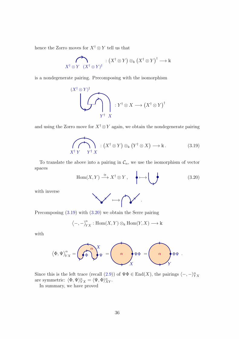
hence the Zorro moves for X† ⊗ Y tell us that
(X† ⊗ Y )†X† ⊗ Y:(X† ⊗ Y
)⊗k(X† ⊗ Y
)† −→ k
is a nondegenerate pairing. Precomposing with the isomorphism
Y † X
(X† ⊗ Y )†
: Y † ⊗X −→(X† ⊗ Y
)†
and using the Zorro move for X†⊗Y again, we obtain the nondegenerate pairing
Y †Y XX†:(X† ⊗ Y
)⊗k(Y † ⊗X
)−→ k . (3.19)
To translate the above into a pairing in Cα, we use the isomorphism of vectorspaces
Hom(X, Y )∼=−→ X† ⊗ Y , 7−→ (3.20)
with inverse
7−→ .
Precomposing (3.19) with (3.20) we obtain the Serre pairing⟨−,−
⟩αY X
: Hom(X, Y )⊗k Hom(Y,X) −→ k
with
⟨Φ,Ψ
⟩αY X
=α X
Φ Ψ = α
X
ΨΦ = α
Y
ΦΨ .
Since this is the left trace (recall (2.9)) of ΨΦ ∈ End(X), the pairings 〈−,−〉αY Xare symmetric: 〈Φ,Ψ〉αY X = 〈Ψ,Φ〉αXY .
In summary, we have proved
36

Theorem 3.6. Let B be a bicategory satisfying Assumption 3.1. Then for everyα ∈ B, the category B(O, α) naturally has the structure of a Calabi-Yau categorywith pairing
⟨−,−
⟩αY X
: Hom(X, Y )⊗k Hom(Y,X) −→ k ,⟨Φ,Ψ
⟩αY X
= α
Y
ΦΨ .
Recall that for the closed sector Aα = End(1α) in Section 3.1, the nondegener-ate pairing (3.2) was the ‘sphere correlator projected to a disc’. But in the opensector the role of the sphere correlator is played by the disc correlator – so wecould have guessed the result of Theorem 3.6 from the start!
3.3.2 Open/closed sector
We continue to work with a bicategory B satisfying Assumption 3.1. For everyα ∈ B we have already obtained a commutative Frobenius algebra Aα = End(1α)and a Calabi-Yau category Cα = B(O, α). According to Theorem 3.5, we alsoneed maps
βX : Aα End(X) : βX
for all X ∈ Cα in order to associate an open/closed TQFT to α. In the graphicalcalculus, intuition about these maps becomes a rigorous definition: we set thebulk-boundary map to be
βX : End(1α) −→ End(X) ,
α
φ 7−→α
φ
X
, (3.21)
and the boundary-bulk map is
βX : End(X) −→ End(1α) ,
α
Ψ
X
X
7−→X
Ψ
α
. (3.22)
We have to check that the maps βX , βX satisfy the three conditions (i)–(iii)
in Theorem 3.5. The first one is easy: βX is manifestly an algebra map into thecentre, thanks to the coherence theorem behind the graphical calculus.
To prove conditions (ii) and (iii), we make one additional assumption. Formotivation, recall that we obtained the nondegenerate pairing 〈−,−〉α on Aα
37

in (3.2) by projecting an α-decorated sphere onto a plane. Now we consider asphere with two incoming boundary circles cut out, together with a D-decorateddefect line which separates two phases labelled α and β as follows:
β αD
By isotopically deforming the defect line we obtain the identity
=
in the defect bordism category. Hence we expect the following property for thebicategory B = BZ associated to a defect TQFT:
Assumption 3.7. For every D ∈ B(α, β) and Ψ ∈ End(D), the pairings 〈−,−〉αon End(1α) satisfy
⟨βα
D
Ψ
⟩α
=
⟨α β
D
Ψ
⟩β
, (3.23)
where we write 〈φ〉α for 〈φ, 1〉α.
Under this assumption we can verify condition (ii) of Theorem 3.5 in just oneline. Let φ ∈ End(1α), X ∈ B(O, α) and Ψ ∈ End(X). Then
⟨βX(φ),Ψ
⟩XX
=
X
βX(φ)Ψ =
⟨X
βX(φ)Ψ
⟩O
=
⟨X
Ψφ
⟩α
=⟨φ, βX(Ψ)
⟩c
so indeed βX and βX are adjoint with respect to one another.
At last we prove the Cardy condition. Let X, Y ∈ B(O, α), Φ ∈ End(X) andΨ ∈ End(Y ). Then
⟨βX(Φ), βY (Ψ)
⟩α
(3.22)=
⟨X
Φ
Y
Ψ
⟩α
38
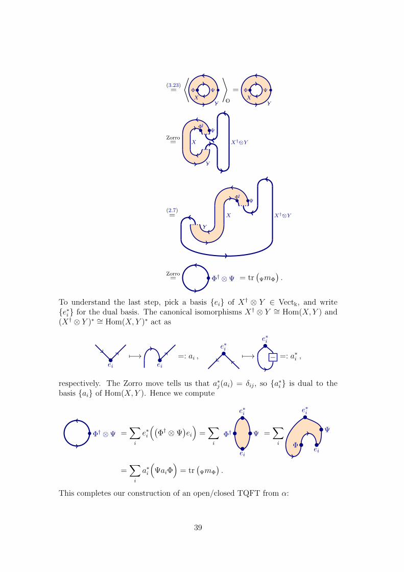
(3.23)=
⟨Y
Ψ
X
Φ
⟩O
=
Y
Ψ
X
Φ
Zorro= X
Y
X†⊗Y
ΨΦ†
(2.7)= X
Y
X†⊗Y
ΨΦ†
Zorro= Φ† ⊗Ψ = tr
(ΨmΦ
).
To understand the last step, pick a basis ei of X† ⊗ Y ∈ Vectk, and writee∗i for the dual basis. The canonical isomorphisms X† ⊗ Y ∼= Hom(X, Y ) and(X† ⊗ Y )∗ ∼= Hom(X, Y )∗ act as
ei
7−→ei
=: ai ,e∗i
7−→ −
e∗i
=: a∗i ,
respectively. The Zorro move tells us that a∗j(ai) = δij, so a∗i is dual to thebasis ai of Hom(X, Y ). Hence we compute
Φ† ⊗Ψ =∑i
e∗i
((Φ† ⊗Ψ
)ei
)=∑i
e∗i
ei
Φ† Ψ =∑i
e∗i
ei
Ψ
Φ
=∑i
a∗i
(ΨaiΦ
)= tr
(ΨmΦ
).
This completes our construction of an open/closed TQFT from α:
39

Theorem 3.8. Let B be a bicategory satisfying Assumptions 3.1 and 3.7. Thenby the above construction for every α ∈ B we have that
• End(1α) has the structure of a commutative Frobenius algebra,
• B(O, α) has the structure of a Calabi-Yau category,
• for every X ∈ B(O, α), the maps βX : End(1α) End(X) : βX of (3.21)and (3.22) satisfy the conditions in Theorem 3.5.
References
[AN] A. Alexeevski and S. Natanzon, Non-commutative extensions oftwo-dimensional topological field theories and Hurwitz numbersfor real algebraic curves, Selecta Mathematica 12 (2006), 307,[math.GT/0202164].
[AS] M. Ando and E. Sharpe, Two-dimensional topological field theories astaffy, Adv. Theor. Math. Phys. 15 (2011), 179–244, [arXiv:1011.0100].
[Ati] M. Atiyah, Topological quantum field theories, Inst. Hautes EtudesSci. Publ. Math. 68 (1988), 175–186.
[BFK] M. Ballard, D. Favero, and L. Katzarkov, A category of kernelsfor equivariant factorizations and its implications for Hodge theory,[arXiv:1105.3177v3].
[BMS] J. Barrett, C. Meusburger, and G. Schaumann, Gray categories withduals and their diagrams, [arXiv:1211.0529].
[BHLW] A. Beliakova, K. Habiro, A. L. Lauda, and B. Webster, Cyclicity forcategorified quantum groups, [arXiv:1506.04671].
[Ben] J. Benabou, Introduction to bicategories, Reports of the Midwest Cat-egory Seminar, pages 1–77, Springer, Berlin, 1967.
[BCP1] I. Brunner, N. Carqueville, and D. Plencner, Orbifolds and topologicaldefects, Comm. Math. Phys. 315 (2012) 739–769, [arXiv:1307.3141].
[BCP2] I. Brunner, N. Carqueville, and D. Plencner, Discrete torsion defects,Comm. Math. Phys. 337 (2015), 429–453, [arXiv:1404.7497].
[CW] A. Caldararu and S. Willerton, The Mukai pairing, I: a categori-cal approach, New York Journal of Mathematics 16 (2010), 61–98,[arXiv:0707.2052].
40

[CMS] N. Carqueville, C. Meusburger, and G. Schaumann, 3-dimensional de-fect TQFTs and their tricategories, [arXiv:1603.01171].
[CM1] N. Carqueville and D. Murfet, Computing Khovanov-Rozansky ho-mology and defect fusion, Algebraic & Geometric Topology 14 (2014),489–537, [arXiv:1108.1081].
[CM2] N. Carqueville and D. Murfet, Adjunctions and defects in Landau-Ginzburg models, Advances in Mathematics 289 (2016), 480–566,[arXiv:1208.1481].
[CQV] N. Carqueville and A. Quintero Velez, Calabi-Yau completion andorbifold equivalence, [arXiv:1509.00880].
[CRCR] N. Carqueville, A. Ros Camacho, and I. Runkel, Orbifold equivalentpotentials, Journal of Pure and Applied Algebra 220 (2016), 759–781,[arXiv:1311.3354].
[CR] N. Carqueville and I. Runkel, Orbifold completion of defect bicate-gories, Quantum Topology 7:2 (2016) 203–279, [arXiv:1210.6363].
[Cos] K. J. Costello, Topological conformal field theories and Calabi-Yau categories, Advances in Mathematics 210:1 (2007), 165–214,[math.QA/0412149].
[DKR] A. Davydov, L. Kong, and I. Runkel, Field theories with defects andthe centre functor, Mathematical Foundations of Quantum Field The-ory and Perturbative String Theory, Proceedings of Symposia in PureMathematics, AMS, 2011, [arXiv:1107.0495].
[DM] T. Dyckerhoff and D. Murfet, Pushing forward matrix factori-sations, Duke Mathematical Journal 162:7 (2013), 1249–1311,[arXiv:1102.2957].
[EGNO] P. Etingof, S. Gelaki, D. Nikshych, and V. Ostrik, Tensor categories,Mathematical Surveys and Monographs 22, American MathematicalSociety, 2015.
[FFRS] J. Frohlich, J. Fuchs, I. Runkel, and C. Schweigert, Defect lines, duali-ties, and generalised orbifolds, XVIth International Congress on Math-ematical Physics, World Scientific, 2009, 608–613, [arXiv:0909.5013].
[HSV] J. Hesse, C. Schweigert, and A. Valentino, Frobenius algebrasand homotopy fixed points of group actions on bicategories,[arXiv:1607.05148].
41

[FHK] M. Fukuma, S. Hosono, and H. Kawai, Lattice Topological Field The-ory in Two Dimensions, Comm. Math. Phys. 161 (1994), 157–176,[hep-th/9212154].
[HKK+] K. Hori, S. Katz, A. Klemm, R. Pandharipande, R. Thomas, C. Vafa,R. Vakil, and E. Zaslow, Mirror symmetry, Clay Mathematics Mono-graphs 1, American Mathematical Society, 2003.
[JS] A. Joyal and R. Street, The geometry of tensor calculus I, Advancesin Mathematics, 88:1 (1991), 55–112.
[Kap] A. Kapustin, Topological Field Theory, Higher Categories, and TheirApplications, Proceedings of the International Congress of Mathemati-cians, Volume III, Hindustan Book Agency, New Delhi, 2010, 2021–2043, [arXiv:1004.2307].
[KS] G. M. Kelly and R. Street, Review of the elements of 2-categories,Category Seminar (Proceedings Sydney Category Theory Seminar1972/1973), Lecture Notes in Mathematics 420, pages 75–103,Springer, 1974.
[KL] M. Khovanov and A. D. Lauda, A diagrammatic approach to cate-gorification of quantum groups I, Representation Theory 13 (2009),309–347, [math.QA/0803.4121].
[KR] M. Khovanov and L. Rozansky, Matrix factorizations and link homol-ogy, Fund. Math. 199 (2008), 1–91, [math.QA/0401268].
[Koc] J. Kock, Frobenius algebras and 2D topological quantum field theories,London Mathematical Society Student Texts 59, Cambridge UniversityPress, 2003.
[Lau1] A. D. Lauda, A categorification of quantum sl2, Advances in Mathe-matics 225 (2008), 3327–3424, [arXiv:0803.3652].
[Lau2] A. D. Lauda, An introduction to diagrammatic algebra and categorifiedquantum sl2, Bulletin of the Institute of Mathematics Academia Sinica(New Series) 7:2 (2012), 165–270, [arXiv:1106.2128].
[LP1] A. D. Lauda and H. Pfeiffer, Two-dimensional extended TQFTs andFrobenius algebras, Topology and its Applications 155:7 (2008), 623–666, [math.AT/0510664].
[LP2] A. D. Lauda and H. Pfeiffer, State sum construction of two-dimensionalopen-closed Topological Quantum Field Theories, J. Knot Theor. Ram-ifications 16 (2007), 1121–1163, [math.QA/0602047].
42

[Laz] C. I. Lazaroiu, On the structure of open-closed topological field the-ory in two dimensions, Nucl. Phys. B 603 (2001), 497–530, [hep-th/0010269].
[MS] G. W. Moore and G. Segal, D-branes and K-theory in 2D topologicalfield theory, [hep-th/0609042].
[Rou] R. Rouquier, 2-Kac-Moody algebras, [arXiv:0812.5023].
[Sar] G. Sarkissian, Defects in G/H coset, G/G topological field theory anddiscrete Fourier-Mukai transform, Nuclear Physics B 846:2 (2011),338–357, [arXiv:1006.5317].
[SP] C. Schommer–Pries, The Classification of Two-Dimensional ExtendedTopological Field Theories, PhD thesis, UC Berkeley (2009),https://sites.google.com/site/chrisschommerpriesmath.
[Shu] M. A. Shulman, Constructing symmetric monoidal bicategories,[arXiv:1004.0993].
[Toe] B. Toen, Lectures on DG-Categories, Topics in Algebraic and Topo-logical K-Theory 2008 (2011), 243–302, [arXiv:1202.6292].
[Weh] K. Wehrheim, Floer Field Philosophy, [arXiv:1602.04908].
43