Lecture Notes – Introduction

Why is the study of the Health Care System interesting/important?• Interesting Facts

• Personal health care expenditures trends (see Table 1):

• 17.9% of GDP in 2011• 50% of per capita GDP in 2011• Part of this is caused by an increase in prices • Part is caused by an increase in real expenditures

• Changing nature of the medical profession:• Move from fee-for-service care to managed care • Increases in medical malpractice • These Δs partially caused by increase in expenditures • Disease management (attempt to reduce costs by

providing experts by insurance companies to help manage diseases – decrease risky behavior, increase preventative medicine.

How does economics help?• Positive verses Normative Issues

• Positive analysis = analysis of how the world works

• Objective• Factual• Testable (if true/false therefore must be positive) • Example = Is a market outcome efficient?

• Normative analysis = analysis of how the world should work

• Subjective or opinions• Not testable• Example = all market outcomes should be efficient.

• What other important examples can you think of?

Economic Analysis• You have scarcity so you

must make choices.

• This concept is illustrated by the production possibility frontier (PPF) in the graph. • As you can see, an

increase in medical services necessarily involves a decrease in the consumption of other goods.

• From Graph 2 analysis, you can conclude: • Even if you devote all

resources to medical care you may NOT be able to reach 100% on x-axis (ie. intersection = point like A not B)

• You cannot have both high consumption of other goods + NHI (w/ high quality care) → must be a rationing device!

Graph 2

• Example: National Health Insurance in other countries• Positive Analysis: rationing is done by time

rather than price as in the U.S. (or employment etc.)

• Normative Analysis: they have NHI, but scarcity still exists

• What are other considerations given scarcity?

Where is the Net Benefit to Society Highest?• Consider the following:

• To maximize net benefit, set % such that Marginal Benefit (MB) = Marginal Cost (MC) → setting a high % may necessarily mean setting % less than 100%. In other words, it is probable that some individuals have a benefit to society of insuring a low cost.

• Example: • Most individuals who would benefit to

society by having insurance won’t insure themselves and IF they do it will be inefficient.

• How? Well, society could gain benefit by spending money on other programs such as: • Pre-natal care• Informational programs• Police protection• Food assistance• Education

• → Is such a conclusion moral?

The Economic Tools- A Brief Overview

• 4 major areas we will discuss: • Demand and Supply• Cost Curves & Π Max • Consumer Choice• Theory of the Firm

Demand• Q. What is the definition of

demand?• A. The amount of a

good/service a consumer/market is willing and able to buy (Qd) in a given time period given the price, ceteris paribus (all else equal).

• Q. What is the law of demand• A. The lower a goods price the

higher Qd , all else equal, and reverse.

• Shifts in demand caused bychanges in: • Tastes• Income • Price of related goods• # of buyers• Expectations• Make sure you know how these all work.

Supply• Q. What is the

definition of supply?• A. The amount of a

good a firm is willing and ABLE to supply (Qs) given the price, ceteris paribus

• Q. What is the law of supply?

• A. ↑P → ↑ Qs , all else equal, and reverse.

• Shifts in supply caused by• Costs of production

• Affected by Technology and input prices

• Price of related goods• Substitutes • Complements

• Number of suppliers• Expectations

• Make sure you know how all these work.

Equilibrium • What happens if • D↑ ?? → P↑ & Q↑ • D↓ ?? → P↓ & Q↓ • S↑ ?? → P↓ & Q↑ • S↓ ?? → P↑ & Q↓ • D↑ & S↑ ?? → • D↓ & S↓ ?? → • D↑ & S↓ ?? → • D↓ & S↑ ?? → • The point is to predict P

and Q. Make sure you can.

Elasticity• Elasticity:

• Similar to the concept of a rubber band• The rubber band is more elastic, for the same force

applied, if the band stretches more – vice versa.

• It is a measure of responsiveness

• Price elasticity of Demand = η • η = (%ΔQD)/(%ΔP)

• Measures how responsive D is for a good to a change in the P of that good.

• |η| > 1 or | (%ΔQD)| > |(%ΔP) | => elastic

• |η| < 1 => inelastic• |η| = 1 => unitary elastic

• What does it mean when I say that D is relatively price elastic?• | η |>1 or |%ΔQD| > |%ΔP|

• Same for other types of elasticities:• Supply elasticity

• η s = (%ΔQS)/(%ΔP)

• Income elasticity• η Y = (%ΔQD)/(%ΔY)

• Cross-price elasticity • η xz = (%ΔQD

X)/(%ΔPZ)

Elasticity Graph

Efficiency• Technological Efficiency:

• A firm is able to produce the maximum output given the resources available or

• Given the output produced the minimum resources (costs) are used.

• Allocative Efficiency:• A firm is able to produce at an output

level where P (MSB) = MC (MSB).

Allocative Efficiency Graph

Allocatively efficient if Q=Q* where MSB = MSC.

Applications of D & S 1.Without health

insurance• At EQ = E1 (P1 , MC1)

2. With health insuranceDeadweight loss to

Society

• With Health Insurance• What is happens to D & S?

• P↓ to Consumers to PH

• QD↑ to MCH

• P↑ to Suppliers to PSQS ↑ to MCH

• Is the market in Equilibrium?• Yes (as long as P↑ for suppliers)

• Efficient? Is MSC = MSB • No=> Produce too much => Dead weight loss

to society as long as D = MSB & S = MSC

Consumer Choice & Budget Constraints

• Consumer choice model is a very simple model with only 2 goods to consume: good 1 & good 2.• Quantities = X1 & X2

• Prices = P1 & P2

• M = income• Budget Constraints

• P1X1 + P2X2 ≤ M shows all combinations of goods 1 & 2 that are feasible. Note: P1X1 = $ spent on good 1, P2X2 = $ spent on good 2.

Budget Line• P1X1 + P2X2 = M , i.e. spend all your money

• Now look at the Budget Line more closely?

1.What is the maximum amount of good 1 that can be consumed? = M/P1

2.Same for good 2 = M/P23.What is the (opportunity) cost of more

X1 (or X2)?• Suppose P1 = 2 and P2 = 1. What is the

cost of X1 = ? 1 more X1 => must give up 2 units of X2

• Slope of Budget Line = -(P1/P2) = opportunity cost of good 1 = 1/2

• What is the opportunity cost of good 2 = ? = - (P2/P1) = 2/1

• → get:

• Note: Since given by P1X1 + P2X2 = M. Put into slope intercept form by solving for X2

→ P2X2 = M - P1X1 or

→ X2 = (M/P2)- (P1/P2) where (M/P2) is the intercept and -(P1/P2) is the slope

Changes in the Budget LinePricesIncome

Preferences & Utility• Pick 3 consumption bundles X, Y, and Z

Preferences• Define preferences:

• If X Y → X is ‘strictly preferred’ to Y≻• If X Y → X is ‘weakly preferred’ to Y≿• If X ∼ Y → X is ‘indifferent’ with Y

• Assume individuals are rational which means:• Completeness: Either X Y or Y X≿ ≿• Reflexivity: X X≿• Transitivity: If X Y and Y Z >> X Z≿ ≿ ≿

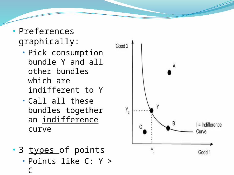
• Preferences graphically:• Pick consumption

bundle Y and all other bundles which are indifferent to Y

• Call all these bundles together an indifference curve

• 3 types of points• Points like C: Y C≻• Points like B: Y ∼ B• Points like A: A Y ≻

• Individual curves facts:1. Cannot cross (violates transitivity)2. Infinite family of individual curves

• Examples of types of individual curves: 1. Perfect substitutes2. Perfect complements3. Bads4. Neutral Goods5. Satiation Points

Perfect Substitutes – person views the two goods as exactly

the same. Move in the direction of the arrow increases preferences.

Perfect Complements – need the two goods together in a fixed ratio.

Bads – more of a bad makes one worse off

Neutral Goods – x1 good, x2 neutral – increase a neutral and neither better or worse off.

Satiation Point = S, at S each good changes between good and bad.

• We will generally assume that preferences look like this:

• i.e. Averages are preferred to extremes convexity

Utility• Utility assumptions:

1. That individuals have preferences

2. Utility measures those preferences in such a way that if W X Y Z → ≻ ≻ ≻U(W) U(X) U(Y) U(Z)≻ ≻ ≻

• What happens as we move out to higher indifference curves → utility levels ↑

• Utility assumptions continued: • 3. We assume that individuals want to maximize utility

given: • Prices• Income• Preferences

• 4. Marginal Utility=MU• MU1= (Δ Total Utility1) / (ΔX1)• MU2= (Δ Total Utility2) / (ΔX2)

• Marginal Rate of Substitution: MRS• Rate at which consumer is willing to substitute 1 good

for another• slope of indifference curve• -MU1/MU2

Budget Line & Preferences• Put together a budget line and preferences:

• Choose point A for maximum utility. Why?• It is where -p1/p2=MRS=-MU1/MU2

Consumer Demand• Consumer demand

is derived from all the individual demands in the market for the two goods.

→ Individual demand is derived from utility analysis.

• Example: Subsidies of health by the government• Suppose the government has 2 goals

• Supply low-cost health care to the aged• Do not subsidize other goods

• Now consider some different plans• 1. The entire cost of medical care is paid for

by all program participants. • Conclusion:

• Supplies low-cost but participants over consumer i.e. choose HC until MCHC=0

• Does subsidize other goods. How?• Very costly

Plan 1 Graph

• Different plans continued: • 2. The government pays a lump-sum payment of

$M1

• Conclusion:• May supply low-cost but MCHC < MC2 → may mostly

supply other goods• Cost is contained unless number of participants is

high

• Different plans continued: • 3. Lump sum payment of $M1 but must be spent on

health

• Conclusion:• Everyone buys at least M1/PH HC• If HC = 0 before → no subsidy of other goods• If HC > 0 before → subsidy of other goods (Why?)• Enforcement costs

• Different plans continued: • 4. The government subsidizes the price of health

care by paying some % of the price

• Conclusion:• Even with the subsidy individuals may (depends

on MCHC) buy very little, if any, more HC - especially if very poor

• Will subsidize other goods• Cost?

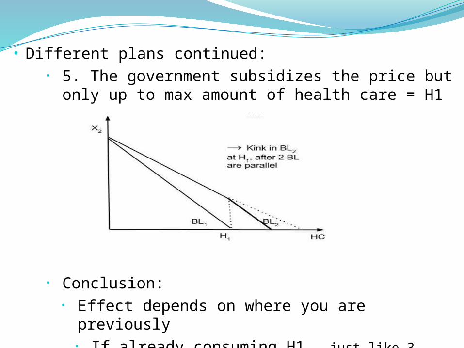
• Different plans continued: • 5. The government subsidizes the price but only

up to max amount of health care = H1

• Conclusion:• Effect depends on where you are previously

• If already consuming H1 → just like 3

• If not → just like 4

• Three Questions to think about• 1. Which plan is the best?

• 2. Are there any other programs that could be analyzed?

• 3. What value does the model have? OR Can you do the same thing without the model?

Production & Profit Maximization• What is the production process?

• When inputs combined together in the production process( i.e. technology) yields an output.

• Inputs include • Land- natural resources• Labor (L)• Capital (K)• Entrepreneurship

Production Function• The production process is often called

the production function where Q(output)= f(inputs)

• To make it simple and assume only 1 variable input = labor (L) and a fixed input (K)

• Production function shows the relationship between labor and output

• What is that relationship?

Production Function• Three types of points

• A= given resources, can't produce this much

• C= given resources, can produce Qc but are technologically inefficient

• B= given resources, are producing the max. Output → Technologically efficient!

• Define • MPL = Δ Q/ Δ L

• APL = Q/L • Note Kbar indicates capital is fixed.

• Can do the same for any other input like capital (K)

• Look at the shape of the production function on the graph i.e. law of diminishing marginal productivity

• From this derive the short-run cost curves • → get the following

Identities & Definitions• TC = TVC + TFC

• AC = TC/Q = AVC + AFC

(from TC)

• AVC = TVC/Q

• AFC = TFC/Q

• MC = Δ TC/Δ Q = Δ TVC/Δ Q + Δ

TFC/Q = Δ TVC/ Δ Q

• Where • TC: Total Cost• TVC: Total Variable

Cost• TFC: Total Fixed Cost• AC: Average Cost• AVC: Average Variable

Cost• AFC: Average Fixed

Cost• MC: Marginal Cost

Cost CurvesQ. Why do the cost curves look as

they do?A. Assumptions about the underlying

short-run production functionThe main one is diminishing marginal productivity

Π maximization Marginal revenue (MR)

Marginal Revenue MR= Δ TR/ Δ QIf industry P.C. → MR = P In the graph, see where it produces MR=MC to

max Π.

For a monopoly the cost curve is the same for all but It only faces outline market demandStill Π-max by producing where MR = MC

Main points 1. If on cost curves →

Technologically efficient2. Π-maximizing firms always on cost

curves3. But does the industry produce at

minimum point of AC curve?Not necessarily

Technological Efficiency2 kinds of technological efficiency:

Firm is technology efficient if given output producing it at minimum cost (i.e. on the cost curves)

Industry is technologically efficient if given output → at minimum cost → producing at minimum point on AC curve

This analysis is short-run. Now look at long-run where all inputs are variable.

Assume 2 inputs K & L So Q = f(K, L) before either K = Kbar or L = LbarNow both are free to changeHow does the firm decide how much K & L to use to produce Q?

Statistical Tools Hypothesis testing

Ever heard an factual assertion and wondered if its true? Can you think of any? For example, male wages exceed female wages

1st step in testing is to set up an hypothesis Null hypothesis→ one we wish to disprove

WM = WF

Alternative hypothesis → several are possible WM > WF

WM ≠ WF

WM < WF

How to test?1st possibility is to look at means

Mean of distribution= Σ Xi/ N = Suppose we calculate M and F find that M > F

Is the null hypothesis false? Could just be random? Want to make sure the likelihood of this being a

random outcome is low Use a measure of dispersion:

Variance = V = Standard deviation = s = Standard Error = SE = s/ ( Actual )

Should have normal distribution – what does that mean?

How to use to test the hypothesis?Calculate M - F / SE

Use the Combined SE or the weighted averageWeighted by sample sizes of men vs. women

Actual FormulasSw = weighted standard deviation

= [(N1- 1)S12 + (N2- 1)S2

2 ) / N1+N2 -2)]T-statistic = [(Xbar1- Xbar2)/ (Sw ( 1/N1 +

1/N2)1/2)] Sw ( 1/N1 + 1/N2)1/2 is weighted standard error OR basically

measure how many standard errors +/- from 0 is the difference between the two wages.

Rule of thumb = 2 S.C. +/- means good evidence that the two means

are different ( although could still happen by chance 5% of the time)

Regression AnalysisSuppose we find the 2 means are different. Why

are the 2 means different?Could be for a number of different reasons or

variables These reasons/variables could be continuous,

that is change continuously → Regression Analysis deals with both issues

1. Deals with both continuous and discrete data2. Controls for other variables

Example: Suppose you have 2 variables. Each dot in the graph below represents an observation.What is the relationship?

A Regression fits the best line thru data points→ yields Health = B0 + B1(H.E.) where Bo is the intercept and B1 is the sl0pe

Generally use OLS, Ordinary Least Squares, to estimate lineMultiple regression analysis with lots of

explanatory variablesY = Bo + B1X1 + B2X2 +…+ BnXn with all else

equalOR

Health = B0 + B1( H.E.) + B2( EDUC) with all else equalMostly I want you to be able to interpret

the coefficients, B0 , B1 , etc.

Dummy variables may also be used.Give the observation a place holder of

0 or 1. For example, 0 for male & 1 for female.

Tests of significanceNote that here the test is whether the

coefficient is zero. That is the null hypothesis is B1 = 0; test statistic is B1/SE = measures how many standard errors from 0 is B1. Again, testing whether an observed B1 that is different from 0 could have occurred randomly. Rule of thumb = 2 SE from 0 (i.e., 5% chance it happened randomly.)

Chapter 4- Cost/Benefit AnalysisProblem in decision making-Which is best

choice?3 approaches

1. CBA = cost benefit analysis = measures costs/benefits in $

Problems?

2. CEA = cost effectiveness analysis = measures costs/benefits in terms of “natural” measures

Problems?

3. CUA = cost utility analysis = changes CEA to measure benefits in terms of preferences

All trying to use society’s viewpoint to make best decisions

CBAHow do firms/individuals behave?

Firms → MR = MCMarginal analysis

MSB = marginal social benefit ( Why ↓ slope? )

MSC = marginal social cost ( Why ↑ slope? )Social optimum when MSB – MSC. Why?

DiscountingWhy is it necessary? What if you pay costs up

front but reap the benefits later?

Discounting cont. You typically want things now rather than later

because you could die tomorrow or you could invest it now and have even more money tomorrow!

Present Discounted Value PV = Σ [( Bt – Ct)/ (1+r)t ]

where B - Benefits , C - Costs, r – interest rate, t - time ( i.e. years)

Cost-BenefitNet benefit = Σ [( Bt – Ct)/ (1+r)t ]

OR B/C = = Σ [(( Bt)/ (1+r)t ) / (( Ct)/ (1+r)t )]

if B/C > 1 → beneficial if B/C = 1 → waste

Discounting cont. Problems Identify B/C in $ Must include external costs How to put $ on B/C Project life/discount rate

What is the discount rate?Given by the opportunities forgone in private sector by project

CBA in Health CareProblems

1. How to value life? (↑ longevity, etc)2. Difficulties in estimating cost

For 1. there are 2 approaches Human capital approach = present value of

future earning Problems?

Willingness to pay to avoid injury Example: CBA of screening tests for STD in

women.

CEACEA or Cost Effectiveness Analysis

Basically ignores benefits and compares only costs of achieving particular objects

Advantages of CEADoable1st step to CBAApplication

CUA & QALYsCUA or Cost Utility Analysis

Special case of CEA uses preferences to rank alternative interventions

QALY or Quality Adjusted Life Years = weighted average of years of life with 1 =

perfect health and 0 = deathUses health status index with weights

determined by individual preferencesExample:

Problems with QALYsSubjectivity - How to get preferences?Equity issuesDistributional issues

Conclusion CUA should use community rather than

individual preferences → How to get preferences or weight?

DALYDALY or Disability Adjusted Life Years

Start with highest achievable life Japanese women= 89.6 years

Then subtract losses from death disabilityYLL = Years Life Lost

Target – Actual for population per age If life expectancy MUs = 76.8 → 89.6 – 76.8 = 12.8

YLD = Years Living with DisabilityDW = Disability Weight

0 = no loss & 1 = death Differs by age