. .

LECTURE NOTES

in

ELEMENTARY COMPLEX FUNCTIONS

with COMPUTER

.

Tadeusz STYS, Ph.D. (Warsaw, 1968)

Professor 1987-2008University of Warsaw 1968-1980Instytute of InformaticsUniversity of Botswana 1980-2008Department of Mathematics

. Gaborone, June 2008

i

PREFACE

These lecture notes are designed for undergraduate students as a comple-mentary text to complex variables with the notebook in Mathematica. It isassumed that students have basic knowledge in real analysis and computing.

The notes has been used in the course on complex variables given to un-dergraduate students at the Faculty of Science, University of Botswana. Theycontain instructions and programs in Mathematica as a system for doing math-ematics with a computer.Each chapter ends with a number of questions that can be used for tutorialsand tests.

Students are encouraged to run the notebook, attached in the appendix,to learn complex variables by solving tutorial questions with Mathematica.

Tadeusz Stys

ii

Contents

1 Revision 1

1.1 Complex Numbers . . . . . . . . . . . . . . . . . . . . . . . . 1

1.2 The Root of z . . . . . . . . . . . . . . . . . . . . . . . . . . . 4

1.3 Logarithm of Complex Numbers . . . . . . . . . . . . . . . . . 6

1.4 Exercises . . . . . . . . . . . . . . . . . . . . . . . . . . . . . . 6

2 Sets on the Complex Plane 9

2.1 Examples of Sets . . . . . . . . . . . . . . . . . . . . . . . . . 9

2.2 Curves on Complex Plane . . . . . . . . . . . . . . . . . . . . 12

2.3 Exercises . . . . . . . . . . . . . . . . . . . . . . . . . . . . . . 13

3 Elementary Functions of a Complex Variable 15

3.1 Definition . . . . . . . . . . . . . . . . . . . . . . . . . . . . . 15

3.2 Linear Function. . . . . . . . . . . . . . . . . . . . . . . . . . 15

3.3 The Power Function zn . . . . . . . . . . . . . . . . . . . . . . 17

3.4 The n − th Root Function . . . . . . . . . . . . . . . . . . . . 18

3.5 The Exponential Function w = ez . . . . . . . . . . . . . . . . 19

3.6 The Logarithmic Function w = ln z. . . . . . . . . . . . . . . 20

3.7 The Trigonometric Functions . . . . . . . . . . . . . . . . . . 23

3.8 The Hyperbolic Functions. . . . . . . . . . . . . . . . . . . . . 24

3.9 The Function w =1

z. . . . . . . . . . . . . . . . . . . . . . . 24

3.10 The Linear Fractional Transformation. . . . . . . . . . . . . . 26

3.11 Exercises . . . . . . . . . . . . . . . . . . . . . . . . . . . . . . 29

4 Continuous and Differentiable Functions 33

4.1 Limits . . . . . . . . . . . . . . . . . . . . . . . . . . . . . . . 33

4.2 Continuity . . . . . . . . . . . . . . . . . . . . . . . . . . . . . 35

4.3 Uniform Continuity . . . . . . . . . . . . . . . . . . . . . . . . 36

4.4 Derivatives . . . . . . . . . . . . . . . . . . . . . . . . . . . . . 37

4.5 Exercises . . . . . . . . . . . . . . . . . . . . . . . . . . . . . . 39

iii

iv

5 Analytic Functions 41

5.1 Cauchy Riemann Equations . . . . . . . . . . . . . . . . . . . 415.2 Definition of Analytic Functions . . . . . . . . . . . . . . . . . 435.3 Liouville’s Theorem . . . . . . . . . . . . . . . . . . . . . . . . 465.4 Fundamental Theorem of Algebra . . . . . . . . . . . . . . . . 465.5 Maximum Modulus Principle . . . . . . . . . . . . . . . . . . 475.6 Exercises . . . . . . . . . . . . . . . . . . . . . . . . . . . . . . 48

6 Integrals 51

6.1 The Integral of a Complex Valued Function of a Real Variable 516.2 Line Integrals . . . . . . . . . . . . . . . . . . . . . . . . . . . 526.3 Antiderivative . . . . . . . . . . . . . . . . . . . . . . . . . . . 556.4 Cauchy Theorem . . . . . . . . . . . . . . . . . . . . . . . . . 566.5 Cauchy Integral Formula . . . . . . . . . . . . . . . . . . . . . 576.6 Cauchy Integral Formula . . . . . . . . . . . . . . . . . . . . 596.7 Cauchy Inequality . . . . . . . . . . . . . . . . . . . . . . . . . 616.8 Morera Theorem . . . . . . . . . . . . . . . . . . . . . . . . . 616.9 Exercises . . . . . . . . . . . . . . . . . . . . . . . . . . . . . . 62

7 Series 67

7.1 Power Series . . . . . . . . . . . . . . . . . . . . . . . . . . . . 677.2 Taylor Series. . . . . . . . . . . . . . . . . . . . . . . . . . . . 707.3 Laurent Series . . . . . . . . . . . . . . . . . . . . . . . . . . . 727.4 Exercises . . . . . . . . . . . . . . . . . . . . . . . . . . . . . . 75

8 Residues 77

8.1 Singular Points . . . . . . . . . . . . . . . . . . . . . . . . . . 778.2 Residues . . . . . . . . . . . . . . . . . . . . . . . . . . . . . . 788.3 Residue Theorem . . . . . . . . . . . . . . . . . . . . . . . . . 818.4 Applications of the Residue Theorem . . . . . . . . . . . . . . 838.5 Exercises . . . . . . . . . . . . . . . . . . . . . . . . . . . . . . 87

Chapter 1

Revision

1.1 Complex Numbers

Every complex number z has the following form:

z = x + iy,

wherex = Re z is the real part of z

y = Im z is the imaginary part of z

i2 = −1 is the imaginary unit.

In Mathematica, real and imaginary parts of a complex number z = x + iyare given by the commands Re[z] and Im[z]. For example, the output of thecommands

z=3+4 I ;

Re[z]^2+Im[z]^2

is 25.A complex number z = x+ iy can be considered as a point (x, y) on the carte-sian plane with the coordinates x and y.

-

@@

@@R

6

x

z = x − iy

Fig 1.1 Complex Plane

0

y z=x+iyr

rφ

−φ

$

%

Trigonometric form of z. Also, every complex number z can be written in

1

2

polar coordinates (φ, |z|), that is

z = |z|(cos φ + i sin φ),

where the modulus |z| =√

x2 + y2 and the argument φ is determined by theequalities

x = |z| cos φ, y = |z| sin φ,

for z 6= 0.In Mathematica, the module and the principal value of argument of z = x+ iyare given by the commands Abs[z] and Arg[z]. For example, the output ofthe commands:

z=1+I;

module=Abs[z];

argument=Arg[z]

are: module=√

2 and argument=π

4.

Conjugate complex number. For any complex number z its conjugate is

z = x − iy.

Thus, in the trigonometric form, the conjugate z = |z|(cos φ − i sin φ) has thesame modulus as z, i.e.

|z| = |z|,and the argument of the conjugate is mines Arg(z), i.e.,

Arg(z) = −Arg(z) = −φ.

One can get the conjugate of z = x + iy, by the Mathematica commandConjugate[z].Exponential form of z. Let z = x + iy, or in trigonometric form

z = |z|(cos φ + i sin φ).

Then, we have the following exponential form of z

z = |z|eiφ,

where eiφ = cos φ + i sin φ.The Mathematica function trigForm prints the trigonometric form of a com-plex number z

trigForm[z_]:=Print[Abs[z],"(Cos ",Arg[z],"+I Sin ",Arg[z],")"];

For example, the command

trigForm[1+I]

3

prints the trigonometric form of z = 1 + i, as follows:√

2(cosπ

4+ I sin

π

4).

The principal argument of z. Let us note that if φ is an argument of zthen φ + 2kπ is also an argument of z for any integer k = 0,±1,±2, ...,The principal argument of z is the unique one which belongs to the interval(−π, π], and is denoted by Arg(z). So that

−π < Arg(z) ≤ π.

Arithmetic operations. We perform four arithmetic operations on the com-plex numbers z1 = x1 + iy1 and z2 = x2 + iy2, according to the following rulesAddition and Subtraction

z1 ± z2 = (x1 + iy1) ± (x2 + iy2) = (x1 ± x2) + i(y1 ± y2),

Multiplication.

z1 ∗ z2 = (x1 + iy1) ∗ (x2 + iy2) = (x1x2 − y1y2) + i(x1y2 + x2y1).

Division.z1

z2=

x1 + iy1

x2 + iy2=

x1x2 + y1y2

x22 + y2

2

+ iy1x2 − y2x1

x22 + y2

2

,

for z2 6= 0.Let us note that multiplying or dividing two complex numbers z1 = |z1|eiφ1

and z2 = |z2|eiφ2 , in exponential forms, we find

z1 ∗ z2 = |z1| |z2|ei(φ1+φ1),

andz1

z2=

|z1||z2|

ei(φ1−φ2),

for z2 6= 0.Power of z. Let us consider z in the exponential form

z = |z|eiφ.

Clearly, the power α of z is

zα = |z|αeiαφ = |z|α(cos αφ + i sin αφ),

for any real number α.In particular, we have De Moivre’s formula

(cos φ + i sin φ)n = cos nφ + i sin nφ = ei nφ,

for any natural n.In order to convert a complex number from its trigonometric form to theexponential form, we can use the Mathematica command TrigToExp[z]. Forexample, the command

4

TrigToExp[Cos[Pi/8]+ I Sin[Pi/8]]

gives the exponential form eIπ

8 .In order to covert a complex number from its exponential form to the trigono-metric form, we use the command ExpToTrig[z]. For example, the command

ExpToTrig[Exp[I Pi/8]]

gives the trigonometric form cosπ

8+ i sin

π

8.

1.2 The Root of z

Every complex number z = x + iy which satisfies the equation

zn = a

is called n-th root of the complex number a = a1 + ia2 and denoted by n√

a.The following theorem holds:

Theorem 1.1 There are exactly n distinct roots of n-th root of a complexnumber a 6= 0. These roots are given by the following formula:

zk = n

√

|a|(cosφ + 2kπ

n+ i sin

φ + 2kπ

n), (1.1)

for k = 0, 1, ..., n − 1., where φ = Arg(a) and n

√

|a| is the arithmetic root ofthe real number |a| .

Proof. Let us consider the complex numbers

z = |z|(cos θ + i sin θ), a = |a|(cos φ + i sin φ).

Clearly, the equationzn = a

takes the trigonometric form

|z|n(cos θ + i sin θ)n = |a|(cosφ + i sin φ).

Hence, by De Moivre’s formula

|z|n(cos nθ + i sin nθ) = |a|(cos φ + i sin φ).

Comparing the modules and arguments, we find

|z| = n

√

|a|, nθ = φ + 2kπ, k = 0,±, 1,±, 2, ...,

Thus, all distinct roots of a are

zk = n

√

|a|(cosφ + 2kπ

n+ i sin

φ + 2kπ

n),

for k = 0, 1, ..., n − 1.

5

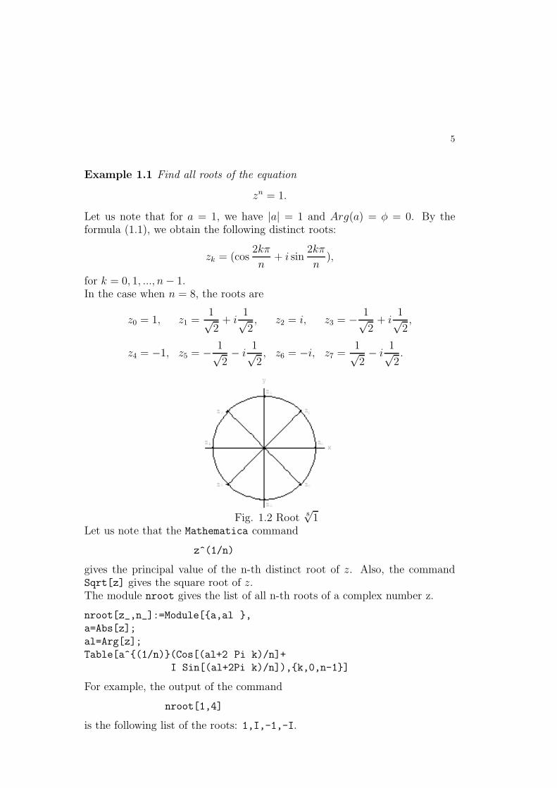
Example 1.1 Find all roots of the equation

zn = 1.

Let us note that for a = 1, we have |a| = 1 and Arg(a) = φ = 0. By theformula (1.1), we obtain the following distinct roots:

zk = (cos2kπ

n+ i sin

2kπ

n),

for k = 0, 1, ..., n − 1.In the case when n = 8, the roots are

z0 = 1, z1 =1√2

+ i1√2, z2 = i, z3 = − 1√

2+ i

1√2,

z4 = −1, z5 = − 1√2− i

1√2, z6 = −i, z7 =

1√2− i

1√2.

Fig. 1.2 Root 8√

1Let us note that the Mathematica command

z^(1/n)

gives the principal value of the n-th distinct root of z. Also, the commandSqrt[z] gives the square root of z.The module nroot gives the list of all n-th roots of a complex number z.

nroot[z_,n_]:=Module[a,al ,

a=Abs[z];

al=Arg[z];

Table[a^(1/n)(Cos[(al+2 Pi k)/n]+

I Sin[(al+2Pi k)/n]),k,0,n-1]

For example, the output of the command

nroot[1,4]

is the following list of the roots: 1,I,-1,-I.

6

1.3 Logarithm of Complex Numbers

Let a 6= 0 be a complex number. Every number z which satisfies the equation

ez = a, ; z = x + iy, (1.2)

is called logarithm of a and denoted by

z = ln a.

The logarithm of a = 0 does not exist.Let us consider a in the exponential form

a = |a|eiφ.

Then, the equation (1.2) is

ez = ex+iy = exeiy = |a|eiφ.

Hence, we get

ex = |a|, x = ln |a|, y = Arg(a) + 2πk, k == 0,±1,±2, ...,

Thus, there are infinite number of logarithms of a complex number a 6= 0which are given by the formula

ln a = ln |a| + i Arg(a) + i 2πk, k = 0,±1,±2, ...,

However, there is only one principal value of the logarithm

ln a = ln|a| + i Arg(a),

which corresponds to the principal argument Arg(a) of a, (k = 0).

Example 1.2 We compute

ln (−1) = ln 1 + iπ + i 2πk = i(2k + 1)π, k = 0,±1,±2, ...,

and the principal value ln(−1) = iπ.

The command Log[z] in Mathematica gives the principal value of the loga-rithm of z. For example, the output of the command Log[-1] is Iπ.

1.4 Exercises

Question 1.1 Evaluate

(i) 8√−1, (ii) 4

√1 + i.

7

Question 1.2 Use Mathematica to evaluate

(i)z2 + 2z + 1

z4 + 2z2 + 1, (ii) (z2 + z + 1) 4

√z,

for z = 1 + i.

Question 1.3 Let a = a1 + ia2 and b = b1 + ib2, be two complex numbersdifferent from zero. For which values of their arguments the product a b and

the quotienta

bare real numbers.

Question 1.4 Prove that

1. (a)z1 ± z2 = z1 ± z2,

(b)z1 z2 = z1 z2,

(c)z1

z2

=z1

z2

, z2 6= 0,

(d)|z1 z2| = |z1| |z2|,

(e)(i) |Re z| ≤ |z|, (ii) |Im z| ≤ |z|

(f)|z1 ± z2| ≤ |z1| + |z2|,

(g)|z1 ± z2|2 = |z1|2 ± 2Re(z1 z2) + |z2|2.

(h) Check the relations (a), (b) and (d) in Mathematica.

Question 1.5 Assume the zk 6= 1 is an n-th root of one. Show that

1 + zk + z2k + . . . + zn−1

k = 0.

Question 1.6 Show that

|1 − z

z − 1| = 1, z 6= 1.

Question 1.7 Show that

|n∑

i=1

zi| ≤n∑

i=1

|zi|.

for complex numbers z1, z2, ..., zn.

8

Question 1.8 Prove that

1. (a)

sin2π

n+ sin

4π

n+ sin

6π

n+ · · · + sin

2(n − 1)π

n= 0,

(b)

cos2π

n+ cos

4π

n+ cos

6π

n+ · · · + cos

2(n − 1)π

n= −1.

for any even n = 2, 4, ...,Hint: Solve the equation zn − 1 = 0.

Question 1.9 Prove the following formula:

1. (a)

cos nφ = cosn φ −(

n

2

)

cosn−2 φ sin2 φ +

(

n

4

)

cosn−4 φ sin4 φ − ...,

(b)

sin nφ =

(

n

1

)

cosn−1 φ sin φ −(

n

3

)

cosn−3 φ sin3 φ +

(

n

5

)

cosn−5 φ sin5 φ − ...,

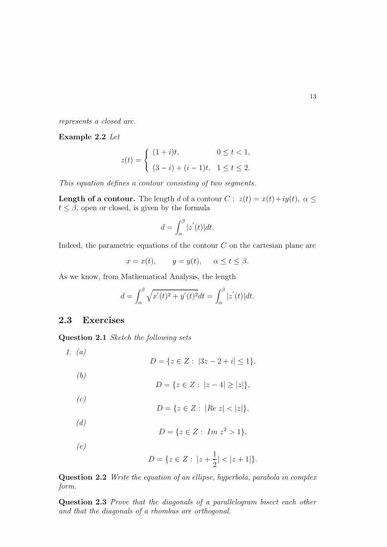
Question 1.10 Sketch the following sets

1. (a)D = z ∈ Z : |z − i| < |z − 1|.

(b)D = z ∈ Z : |z|2 > z + z.

Question 1.11 Show that

1

2|a + b| ≤ max|a|, |b|,

for every complex numbers a and b.

Question 1.12 Show that

| z − a

az − 1| = 1,

for every |z| = 1 and z 6= a.

Question 1.13 Let z = reiθ and w = Reiϕ, where 0 < r < R. Show that

Re(

w + z

w − z

)

=|w|2 − |z|2|w − z|2 =

R2 − r2

R2 − 2rR cos(θ − ϕ) + r2.

Chapter 2

Sets on the Complex Plane

2.1 Examples of Sets

1. (a) Line Segment. For given complex numbers a = a1 + ia2 and b =b1 + ib2, the line segment with the end points a and b is the followingset:

[a, b] = z(t) = (1 − t)a + t b : 0 ≤ t ≤ 1,

-

6

x

Fig 2.1 Line Segment

0

y

a

b

(b) Circle. The circle C(z0, r) with the radius r > 0 and the center atthe point z0 is the set of the points z which satisfy the equation

|z − z0| = r.

Also, the same circle has the following trigonometric equation:

z = z0 + r(cos φ + i sin φ), −π < φ ≤ π,

or exponential equation

z = z0 + reiφ, −π < φ ≤ π.

-

6

x

Fig 2.2 Circle

0

y

&%'$qrz0

φ

9

10

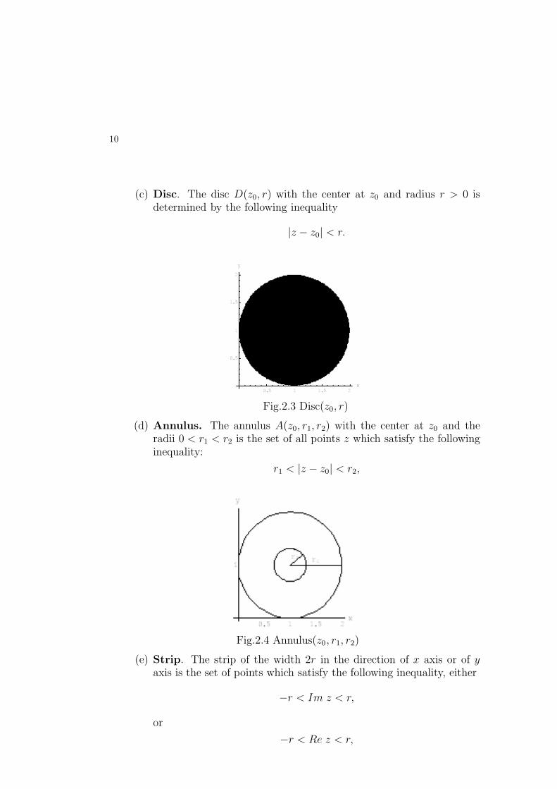
(c) Disc. The disc D(z0, r) with the center at z0 and radius r > 0 isdetermined by the following inequality

|z − z0| < r.

Fig.2.3 Disc(z0, r)

(d) Annulus. The annulus A(z0, r1, r2) with the center at z0 and theradii 0 < r1 < r2 is the set of all points z which satisfy the followinginequality:

r1 < |z − z0| < r2,

Fig.2.4 Annulus(z0, r1, r2)

(e) Strip. The strip of the width 2r in the direction of x axis or of yaxis is the set of points which satisfy the following inequality, either

−r < Im z < r,

or

−r < Re z < r,

11

- -

6 6

x

y

x

y

0 0

−r < Im z < rr

-r

−r < Re z < r

-r r

Fig 2.5 Strip

(f) Sector. The sector with the angle between α and β is the set of allpoints z which satisfy the following inequality:

α < Arg(z) < β,

-

6

@@

@@

@@

z = x + iyqβ

α

x

y

0

Fig 2.6 Sector

Neighborhood. The ǫ− neighborhood of a complex number z0 is the disc

Nǫ(z0, z) = z ∈ Z : |z − z0| < ǫ, ǫ > 0,

12

where Z is the complex plane.Interior, exterior and boundary complex numbers of a set D. Acomplex number z0 is an interior number of the set D, whenever, there issome neighborhood N(z0, z) of z0 which is included in D, that is N(z0, z) ⊂D. The point z0 is an exterior complex number of the set D if there is aneighborhood N(z0, z) which contains no numbers of D. If z0 is neither ofthese, it is then a boundary point of D. Thus, z0 is a boundary number of Dif every neighborhood of z0 contains both interior and exterior numbers of D.Open Set. A set D of complex numbers is open if it consists only of interiornumbers, so that, every number z0 ∈ D belongs to D together with its someneighborhood.Closed Set. A set D of complex numbers is closed if D contains all its interiorand boundary numbers.Let us observe that some sets can be neither open nor closed. For example,the set

D = z ∈ Z : 0 < |z| ≤ 1, is neither open nor closed.Connected Set. An open set D is connected if each pair of numbers z1, z2 ∈D can be joined by a polygonal path consisting of a finite number of linesegments joined end to end which entirely lie in D.Bounded Set. A set D is bounded if there is a disc |z| ≤ R < ∞ whichcontains the set D, otherwise D is an unbounded set.Domain. An open set D which is connected is called domain.

2.2 Curves on Complex Plane

Let x(t) and y(t) be real continuous functions given for t1 ≤ t ≤ t2. Then theparametric equation

C : z(t) = x(t) + iy(t), t1 ≤ t ≤ t2, (2.1)

defines a continuous curve on complex plane joining end points a = z(t1) andb = z(t2). If the end points coincide, that is, a = z(t1) = z(t2) = b, then thecurve is said to be closed.Simple Closed Curve. A continuous closed curve which does not intersectsitself is called simple closed curve.Arc. let us assume that x(t) and y(t) are continuously differentiable realfunctions in the interval [t1, t2]. Then, the curve C given by the equation (2.1)which does not intersect itself is called smooth curve or arc.Contour. A curve which is composed of a finite number of arcs is calledContour.

Example 2.1 The parametric equation of an ellipse on complex plane

z(t) = r1 cos t + i r2 sin t, r2 ≥ r1 > 0, −π < t ≤ π.

13

represents a closed arc.

Example 2.2 Let

z(t) =

(1 + i)t, 0 ≤ t < 1,

(3 − i) + (i − 1)t, 1 ≤ t ≤ 2.

This equation defines a contour consisting of two segments.

Length of a contour. The length d of a contour C : z(t) = x(t)+ iy(t), α ≤t ≤ β, open or closed, is given by the formula

d =∫ β

α|z′

(t)|dt.

Indeed, the parametric equations of the contour C on the cartesian plane are

x = x(t), y = y(t), α ≤ t ≤ β.

As we know, from Mathematical Analysis, the length

d =∫ β

α

√

x′(t)2 + y′(t)2dt =∫ β

α|z′

(t)|dt.

2.3 Exercises

Question 2.1 Sketch the following sets

1. (a)D = z ∈ Z : |3z − 2 + i| ≤ 1,

(b)D = z ∈ Z : |z − 4| ≥ |z|,

(c)D = z ∈ Z : |Re z| < |z|,

(d)D = z ∈ Z : Im z2 > 1,

(e)

D = z ∈ Z : |z +1

2| < |z + 1|.

Question 2.2 Write the equation of an ellipse, hyperbola, parabola in complexform.

Question 2.3 Prove that the diagonals of a parallelogram bisect each otherand that the diagonals of a rhombus are orthogonal.

14

Question 2.4 Represent graphically the set of values of z for which

1. (a)

|z − 3

z + 3| = 2,

(b)

|z − 3

z + 3| < 2,

(c)Re z2 > 1.

Question 2.5 Describe and graph the locus represented by each of the follow-ing equations

1. (a) |z + 2i| + |z − 2i| = 6,

(b) |z − 3| − |z + 3| = 4,

(c) z(z + 2) = 3.

Question 2.6 Find the equation of a line passing through the points z1 = 1+iand z2 = 2 − 3i.

Question 2.7 Show that the equation

|z − 4i| + |z + 4i| = 10

represents an ellipse. Find the equation of this ellipse in the cartesian coordi-nates x and y and polar coordinates (r, φ). Plot the graph of the ellipse withMathematica.

Question 2.8 Show that the equation

z2 + z2 = 2

represents a hyperbola. Find the equation of the hyperbola in the cartesiancoordinates x and y and polar coordinates (r, φ). Plot the graph of the hyperbolawith Mathematica.

Question 2.9 Find an equation of the circle passing through the points 1 − iand 1 + i. Plot the circle with Mathematica.

Question 2.10 Show that the locus of z such that

|z − a||z + a| = a2, a > 0,

is a lemniscate. Write the equation of the lemniscate in polar coordinates. Plotthe graph of the lemniscate with Mathematica.

Chapter 3

Elementary Functions of a

Complex Variable

3.1 Definition

Let D be a set of complex numbers. A function f defined on D is a rule thatassigns to each z ∈ D a complex number w. The complex number w is calledthe value of the function f at the number z, so that, we note

w = f(z), z ∈ D or f : z ∈ D → w ∈ D′

.

The set D is called the domain of the function f , and the set D′of all values

of f(z) is called the image of the set D, that is D′= f(D).

3.2 Linear Function.

Consider the linear function

f(z) = az + b, a 6= 0, z ∈ Z,

where the constant coefficients a = a1 + ia2 and b = b1 + ib2.Clearly, the domain of the linear function f is whole complex plane, and the setof all values of f(z) is also the whole complex plane. Thus, f(z) maps complexplane onto itself. Let us note that the linear function f(z) = az + b, a 6= 0, isone to one mapping. Indeed, to show this, we observe that

f(z1) = f(z2)

if and only if z1 = z2. Since, the equality

az1 + b = az2 + b

implies z1 = z2 if a 6= 0.Translation. The mapping

w = z + b, z ∈ Z,

15

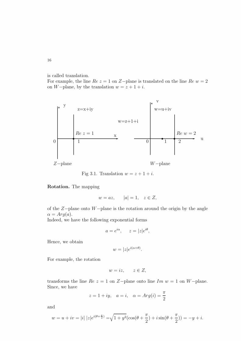
16

is called translation.For example, the line Re z = 1 on Z−plane is translated on the line Re w = 2on W−plane, by the translation w = z + 1 + i.

- -

66

x

yz=x+iy w=u+iv

0 0

Re z = 1s1

w=z+1+i

2s1

s

v

uRe w = 2

Fig 3.1. Translation w = z + 1 + i.

Z−plane W−plane

Rotation. The mapping

w = az, |a| = 1, z ∈ Z,

of the Z−plane onto W−plane is the rotation around the origin by the angleα = Arg(a).Indeed, we have the following exponential forms

a = eiα, z = |z|eiθ,

Hence, we obtain

w = |z|ei(α+θ).

For example, the rotation

w = iz, z ∈ Z,

transforms the line Re z = 1 on Z−plane onto line Im w = 1 on W−plane.Since, we have

z = 1 + iy, a = i, α = Arg(i) =π

2

and

w = u + iv = |i| |z|ei(θ+ π2) =

√

1 + y2(cos(θ +π

2) + i sin(θ +

π

2)) = −y + i.

17

- -

6 6

x

y

0 0

Re z = 1

Im w = 1

Fig. 3.2 Rotation w = iz.

Z−plane W−plane

v

u

z=x+iy w=u+iv

w=iz

In general, the linear mapping

w = az + b, a 6= 0,

is a composition of the rotation

s = az, a 6= 0, z ∈ Z,

and the translation

t = s + b, s ∈ Z,

3.3 The Power Function zn

Let us consider the power function

w = zn, z ∈ D = z ∈ Z : −π

n< Arg(z) ≤ π

n.

for natural n = 1, 2, ...,This function maps a sector D onto whole W−plane. Indeed, let us write thepower function in the following exponential form

w = |z|nenφ, φ = Arg(z),

Clearly, if z ∈ D, that is −πn≤ Arg(z) ≤ π

n, then −π ≤ Arg(w) ≤ π, and

therefore w ∈ W .

18

- -

6

HHHHHHHHHH

πn$

6

x

y

0 0

Fig. 3.3 Power Function w = zn.

Z−plane W−plane

v

u

z = x + iy w = u + iv

w = zn

Let us note that if z moves throughout Z−plane than w reaches n times eachpoint of W−plane. So that, the function is not an one to one mapping. How-ever, the power function is one to one mapping of the sector

Dk = z ∈ Z :(2k − 1)π

n< Arg(z) ≤ (2k + 1)π

n, k = 0, 1, ..., n − 1.

onto whole W−plane.In Mathematica, we compute (x + i y)n, by the command

(x+I y)^n;

3.4 The n − th Root Function

The n − th root function

w = n√

z, z ∈ Z,

has the following exponential form

w = n

√

|z|ei φ+2πk

n , φ = Arg(z), k = 0, 1, ..., n − 1.

Let us note that the n-th root function possesses n different branches fork = 0, 1, ..., n − 1. In the case when k = 0, the function

w = n

√

|z|ei φ

n , φ = Arg(z),

is called Principal Branch of n − th root function.This function maps whole Z−plane onto one of the sectors

Dk = z ∈ Z :(2k − 1)π

n≤ Arg(w) <

(2k + 1)π

n, k = 0, 1, ..., n − 1.

19

On the figure, we present the graph of the sector D0 under principal branchof the n − th root function.

- -

6

@@

@@

πn$

6

x

y

0 0

Fig. 3.4 Root Function w = n√

z.

Z−plane W−plane

v

uD0

z = x + iy w = u + iv

w = n√

z

3.5 The Exponential Function w = ez

Let us prove first the following theorem:

Theorem 3.1 The equationez = 1

holds if and only if z = 2 kπ i, k = 0,±1,±2, ...,.

Proof. For z = x + iy, we have

ez = ex+iy = exeiy = ex(cos y + i sin y) = 1.

Henceex cos y = 1 and ex sin y = 0.

So thatsin y = 0, for yk = kπ, k = 0,±1,±2, ...,

k must be an even integer, since ex cos yk < 0 for odd k. Therefore, the equality

ex cos y = 1

holds for x = 0 and y = 2 π k, and ez = 1 if and only if z = 2 πk i, for anyinteger k.From the theorem, it follows that w = f(z) = ez is a periodic function withthe period ω = 2 π i. Indeed, we have

f(z + 2πi) = ez+2π i = ez e2 π i = ez = f(z).

20

The exponential function w = f(z) = ez is one to one mapping of the strip

D = z = x + iy ∈ Z : −π < y ≤ πonto whole W−plane. Indeed, we have

w = u + iv = ez = ex(cos y + i sin y).

So that −∞ < u = ex cos y < ∞ and −∞ < v = ex sin y < ∞ when −∞ <x < ∞ and −π < y ≤ π. Also, we note that f(z1) = f(z2) if and only ifz1 = z2 when z1, z2 ∈ D. This means that f(z) = ez maps one to one the stripD to whole W−plane.Clearly, f(z) = ez is a periodic function if it is considered on whole Z−plane,since the function maps every strip

Dk = z = x + iy ∈ Z : (2k − 1)π < y ≤ (2k + 1)π, k = 0,±1,±2, ...,

onto whole W−plane.

- -

6 6

x

y

0 0

π

−π

Z−plane W−plane

v

u

z = x + iy w = u + iv

w = ez

Fig. 3.5 Exponential Function w = ez

3.6 The Logarithmic Function w = ln z.

As we know, the exponential function maps one to one every strip

Dk = z = x + iy ∈ Z : (2k − 1)π < y ≤ (2k + 1)π, k = 0,±1,±2, ...,

onto whole W−plane, so that, the inverse function exists and it maps W−plane(without z = 0) onto a strip Dk, k = 0,±1,±2, ...,. This inverse function iscalled logarithmic function and is given by the following formula:

ln z = ln |z| + i(Arg(z) + 2πk), z 6= 0, k = 0,±1,±2, ...,

21

where Arg(z) is the principal value of the argument of z. Let us note that log-arithmic function possesses infinite number of branches. Therefore, w = ln zis a multivalued function if it is considered on the whole complex plane. Thebranch which corresponds to k = 0 is called Principal Branch. Thus, theprincipal branch is given by the following formula:

ln z = ln |z| + iArg(z), z 6= 0.

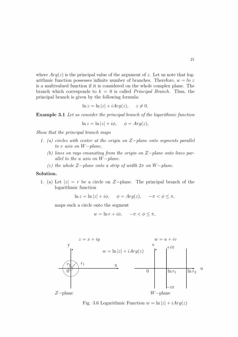
Example 3.1 Let us consider the principal branch of the logarithmic function

ln z = ln |z| + iφ, φ = Arg(z),

Show that the principal branch maps

1. (a) circles with center at the origin on Z−plane onto segments parallelto v axis on W−plane,

(b) lines on rays emanating from the origin on Z−plane onto lines par-allel to the u axis on W−plane.

(c) the whole Z−plane onto a strip of width 2π on W−plane.

Solution.

1. (a) Let |z| = r be a circle on Z−plane. The principal branch of thelogarithmic function

ln z = ln |z| + iφ, φ = Arg(z), −π < φ ≤ π,

maps such a circle onto the segment

w = ln r + iφ, −π < φ ≤ π,

- -

6 6

−iπ

+iπ

ln r1 ln r2&%'$i r1r2 x

y

0 0

Z−plane W−plane

v

u

z = x + iy w = u + iv

w = ln |z| + iArg(z)

Fig. 3.6 Logarithmic Function w = ln |z| + iArg(z)

22

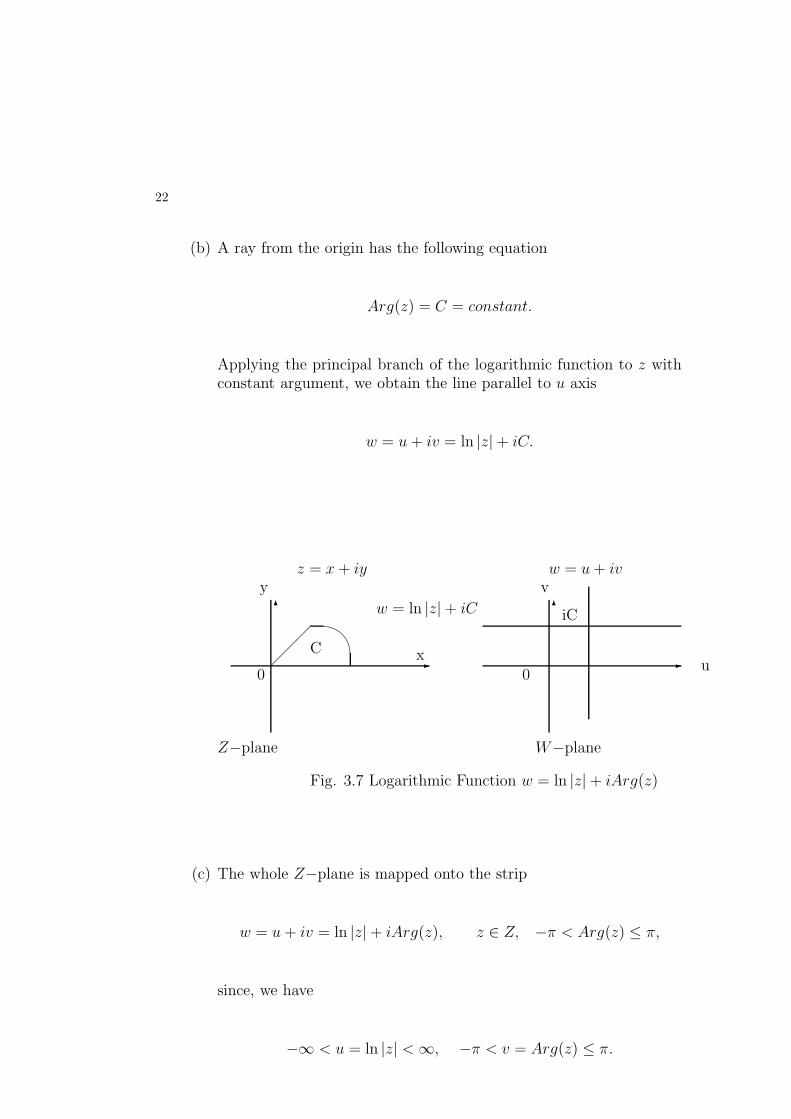
(b) A ray from the origin has the following equation

Arg(z) = C = constant.

Applying the principal branch of the logarithmic function to z withconstant argument, we obtain the line parallel to u axis

w = u + iv = ln |z| + iC.

- -

iC6 6

$

C x

y

0 0

Z−plane W−plane

v

u

z = x + iy w = u + iv

w = ln |z| + iC

Fig. 3.7 Logarithmic Function w = ln |z| + iArg(z)

(c) The whole Z−plane is mapped onto the strip

w = u + iv = ln |z| + iArg(z), z ∈ Z, −π < Arg(z) ≤ π,

since, we have

−∞ < u = ln |z| < ∞, −π < v = Arg(z) ≤ π.

23

- -

+iπ6 6

−iπ

x

y

0 0

Z−plane W−plane

v

u

z = x + iy w = u + iv

w = ln |z| + iArg(z)

Fig. 3.8 Logarithmic Function w = ln |z| + iArg(z)

3.7 The Trigonometric Functions

The trigonometric functions are related with the exponential function by thefollowing formulas:

eix = cos x + i sin x, e−ix = cos x − i sin x,

from which

sin x =eix − e−ix

2i, cos x =

eix + e−ix

2, −∞ < x < ∞.

We define, in the same way, sine and cosine functions of a complex variablez, so that

sin z =eiz − e−iz

2i, cos z =

eiz + e−iz

2, z ∈ Z.

For the trigonometric functions tangent and cotangent, we have formulas

tan z =sin z

cos z=

eiz − e−iz

i(eiz + e−iz), z 6= (2k − 1)

π

2, k = 0,±1,±2, ...,

cot z =cos z

sin z=

i(eiz + e−iz)

(eiz − e−iz), z 6= kπ, k = 0,±1,±2, ...,

24

Let us note some of the properties of trigonometric functions which are knownin a real variable also hold in a complex variable. For example, we have

sin2 z + cos2 z = 1,

sin(−z) = − sin z, cos(−z) = cos z,

tan(−z) = − tan z,

sin(z1 ± z2) = sin z1 cos z2 ± cos z1 sin z2,

cos(z1 ± z2) = cos z1 cos z2 ± sin z1 sin z2, z ∈ Z,

However, modulus of sin z or cos z can exceed one. Indeed, we have

sin 2i = |e−2 − e2

2| > 3,

for z = 2i.

3.8 The Hyperbolic Functions.

The hyperbolic functions sinhz and coshz of a complex variable are given bythe formulas

sinhz =ez − e−z

2, coshz =

ez + e−z

2, z ∈ Z.

These functions satisfy the following identities

cosh2z − sinh2z = 1,

sinh(−z) = −sinhz, cosh(−z) = coshz,

sinh(z1 + z2) = sinh z1 cosh z2 + cosh z1 sinh z2,

cosh(z1 + z2) = cosh z1 cosh z2 + sinh z1 sinh z2.

for all z ∈ Z.

3.9 The Function w =1

z

The function

w =1

z, z 6= 0,

25

is one to one mapping of non-zero numbers on Z−plane onto non-zero numberson W−plane, since

1

z1

=1

z2

if and only if z1 = z2.The exponential form of this function is

w =1

|z|e−iθ, −π < θ ≤ π,

for z = |z|eiθ.Clearly, the function maps a circle

|z| = r, r > 0

onto a circle

|w| =1

r.

Also, under this mapping, the image of the disc

0 < |z| < r,

is the region

|w| >1

r,

outside of the disc on W−plane.

Example 3.2 Find the image of the line

Re z = α 6= 0,

under the mapping

w = u + iv =1

z, z = x + iy.

Sketch the graph.

Solution. Let us note that

w = u + iv =1

z=

x

x2 + y2− i

y

x2 + y2,

Hence, we have

u =x

x2 + y2v = − y

x2 + y2.

and

u2 + v2 =1

x2 + y2=

u

α, for Re z = x = α.

26

By simple modification, we find

u2 − u

α+

1

4α2+ v2 =

1

4α2,

and

(u − 1

2α)2 + v2 = (

1

2α)2.

The above equation represents the circle on W−plane with the center at

w0 =1

2αand the radius r =

1

2α. So that, the function maps the line Re α 6= 0

onto the circle |w − w0| = r.

- -

66

x

yz=x+iy w=u+iv

0 0

Re z = αsα

w =1

z

&%'$s

12α

v

u

Fig. 3.9 The Function w =1

z

Z−plane W−plane

3.10 The Linear Fractional Transformation.

Let us consider the linear fractional mapping

w =az + b

cz + d, ad − bc 6= 0, c 6= 0.

This mapping has the following equivalent form

w =a

c+

bc − ad

c

1

cz + d, ad − bc 6= 0, c 6= 0. (3.1)

The linear fractional transformation is one to one mapping of complex planeonto itself. Indeed, the inequality

az1 + b

cz1 + d=

az2 + b

cz2 + d,

27

holds if and only if z1 = z2. Since then

(az1 + b)(cz2 + d) = (az2 + b)(cz1 + d),

and(ad − bc)(z1 − z2) = 0.

Hence, we have z1 = z2.The inverse to a linear fractional function is also linear fractional function,since we have

z =−dw + b

cw − a, w ∈ W.

A linear fractional function is the composition of a linear function and the

function w =1

z.

Indeed, by the formula (3.1), we have

w = As + B, A =bc − ad

c, B =

a

c, s =

1

t, t = cz + d.

Example 3.3 Show that the equation

|z − p

z − q| = α,

represents a circle for every α > 0, α 6= 1 and p 6= q. Find the center and theradius of the circle.

Solution. By the formula

|a − b|2 = |a|2 + |b|2 − 2Re (ab),

we have

|z − p|2 = |z|2 + |p|2 − 2Re pz = α2(|z|2| + |q|2 − 2Re qz) = α2|z − q|2.After simple operations, we arrive at the following equation

|z|2 − 2Re (p − α2q)z

1 − α2=

−|p|2 + α2|q|21 − α2

.

Adding to both sides the term |p − α2q

1 − α2|2, we obtain the equation

|z − (p − α2q)

1 − α2|2 =

α2|p − q|2(1 − α2)2

.

of the circle with the center at

z0 =p − α2q

1 − α2,

and the radius

r = α|p − q||1 − α2| .

28

Example 3.4 Consider the linear fractional mapping

w =z − z0

z − z0,

where z0 is a fixed point on the upper half of Z−plane, i.e., Im z0 > 0.Show that the function maps one to one the upper half of Z−plane onto unitdisc |w| < 1, on W−plane. Also, show that every point of x axis is mappedonto unit circle |w| = 1.

Solution.

- -

66

x

y s z=x+iy w=u+iv

0 0

Im z = y > 0

z0 = x0 + iy0s w =z − z0

z − z0

&%'$s s

1

v

u

Fig. 3.10 The Function w =z − z0

z − z0

Z−plane W−plane

Let us note that

|w|2 =(x − x0)

2 + (y − y0)2

(x − x0)2 + (y + y0)2≤ 1,

for Im z = y ≥ 0 and Im z0 = y0 > 0.Clearly, the equality |w|2 = 1 holds if and only if y = 0, so that, the x axis(Im z = y = 0) is mapped on the circle |w| = 1.To show that the function is one to one mapping, we observe that the equality

z1 − z0

z1 − z0=

z2 − z0

z2 − z0,

is equivalent to the following equality

(z1 − z2)(z0 − z0) = 0.

Hence, for Imz0 > 0, we get z1 = z2. This means that the linear fractionalfunction is one to one mapping of the upper half of complex plane onto disc|w| ≤ 1.

29

3.11 Exercises

Question 3.1 Find the image of the circle

|z − 1| = 2

under the linear mapping

w = (1 + i)z + 1 − i.

Write the image in polar coordinates and plot it with Mathematica.

Question 3.2 .

1. (a) Let f(z) = z2. Evaluate f(−2 + i) and f(1 − 3i)

(b) Show that the line joining the numbers z1 = −2+ i and z2 = 1− i onZ−plane is mapped into a curve on W−plane joining the numbersw1 and w2. Find the equation of the curve in polar coordinates andplot it with Mathematica.

Question 3.3 Find the image of the hyperbola

(i) x2 − y2 = 1, (ii) xy = 2.

under the mapping w = z2. Plot the image with Mathematica.

Question 3.4 Find the image of the sector

0 < Arg(z) ≤ π

8

under the mappingw = z4.

Sketch the graph.

Question 3.5 .

1. (a) List all branches of the function

f(z) = 3√

z.

(b) Find the image of the region

D = z ∈ Z : Re z ≥ 0, Im z ≥ 0under the principal branch of f(z). Sketch the graph.

Question 3.6 Find the image of the line segment

S = z ∈ Z : Re z = 0, and − π < Im z ≤ π,under the mapping w = ez. Write the image in polar coordinates and plot itwith Mathematica.

30

Question 3.7 .

1. (a) Show that the function

w = f(z) = ez2

,

maps the lines y = x and y = −x onto unit circle |w| = 1.

(b) Show further that f(z) maps each of the two pieces of the region

D = z = x + iy ∈ Z : x2 > y2,

onto the setΩ = w = u + iv ∈ W : |w| > 1.

Question 3.8 . Solve the following equations:

1. (a)

(i) ln z =iπ

6, (ii) ln z = (2n + 1)π i n = 0,±1,±2, ...,

(b)

(i) ez = −1, (ii) ez = −3.

Question 3.9 Find the image of the annulus

2 < |z| ≤ 4,

under the principal branch of the logarithmic function. Sketch the graph.

Question 3.10 Find the image of the sector

1 < Re z ≤ 2,

under the mapping w =1

z, z 6= 0. Sketch the graph.

Question 3.11 Find the image of the line Re z = 3, under the followingmappings:

1. (a)

f(z) =z − 3

z + 3,

(b)f(z) = ez.

Plot the graphs of the images in Mathematica.

31

Question 3.12 Find the image of the line Re z = 2, under the followingmappings:

1. (a)f(z) = z3,

(b)

f(z) =1

z + 2,

(c)

f(z) = lnz − 6

z + 2.

Plot the images with Mathematica.

Question 3.13 Find the fixed points of the mapping

f(z) =2z − 5

z + 4.

Note that: a complex number z is the fixed point of f(z) if z = f(z).

Question 3.14 Solve the following equations:

1. (a)(i) sin z = 1, (ii) cos z = 1.

(b)(i) sin z = 2, (ii) cos z = 2.

Question 3.15 Show that

1. (a)sin z = sin x cosh y + i cos x sinh y, z = x + iy.

(b)| sin z| ≥ | sin x|, z = x + iy.

(c)(i) | sin z|2 = sin2 x + sinh2 y, z = x + iy.

(ii) | cos z|2 = cos2 x + sinh2 y, z = x + iy.

for z = x + iy.

Question 3.16 Find the region onto which the half complex plane Im z =y > 0 is mapped by the transformation

f(z) =1 + i

z,

by using

32

1. (a) Cartesian coordinates

(b) polar coordinates

Sketch the graph.

Question 3.17 Find the linear fractional transformation that maps the com-plex numbers z=2, z2 = i, z3 = −2, onto the numbers w1 = 1, w2 = i, w3 =−1.

Question 3.18 .

1. (a) Show that equation

|z − 2

z + 2| = 4,

represents a circle. Find the center and the radius of this circle.Sketch the graph.

(b) Show that the function

w = f(z) =z − p

pz − 1, |p| 6= 1,

maps one to one

i. the circle |z| = 1 on the circle |w| = 1,

ii. the disc |z| < 1 on the disc |w| < 1 if |p| < 1,

iii. the disc |z| < 1 on the set |w| > 1, if |p| > 1.

Chapter 4

Continuous and Differentiable

Functions

4.1 Limits

Let w = f(z) be a function defined in some neighborhood of a number z0, andnot necessary at z0.

Definition 4.1 A number g is said to be the limit of f(z) at z0, if and onlyif for every ǫ > 0 there exists δǫ(z0) > 0, such that, the inequality

0 < |z − z0| < δǫ(z0)

implies the inequality

|f(z) − g| < ǫ.

If the limit g exists in the sense of this definition, then we apply the followingnotation:

limz→z0

f(z) = g.

We can write the definition in terms of logical quantifies as follows:

∀ǫ>0∃δǫ(z0)>00 < |z − z0| < δǫ(z0) =⇒ |f(z) − g| < ǫ.

Infinite Limit. The limit g of f(z) at z0 is infinite, if for every R > 0 thereexists δR > 0, such that, the inequality

0 < |z − z0| < δR

implies the inequality

|f(z)| > R.

In symbols, we note

limz→z0

f(z) = ∞.

33

34

Limit in Infinity. A function f(z) has a limit g in infinity, if and only if forevery ǫ > 0 there exists Rǫ > 0, such that, the inequality

|z| > Rǫ

implies the inequality

|f(z) − g| < ǫ.

In terms of logical quantifies, we write

∀ǫ>0∃Rǫ>0|z| > Rǫ =⇒ |f(z) − g| < ǫ.

In symbols, we note

limz→∞

f(z) = g.

Example 4.1 Using definition show that

limz→i

2(z2 + 1)

3(z − i)=

4

3i.

Let us note that at z0 = i, the function f(z) =2(z2 + 1)

3(z − i)is not definite,

however f(z) has the limit g =4

3i. Indeed, we consider ǫ > 0 for which

|f(z) − g| = |2(z2 + 1)

3(z − i)− 4

3i| =

2

3|z − i| < ǫ.

Hence, the inequality holds for |z − i| < δǫ =3

2ǫ.

A limit of a complex valued function f(z) at a point z0 in Mathematica isgiven by the command:

Limit[f(z), z− > z0].

For example

Limit[(z- I)/(z^2+1),z->I]

gives −I

2, or

Limit[2(z^2+1)/(3(z-I)), z->I]

gives4I

3

35

4.2 Continuity

Let f(z) be a function definite in a neighborhood of a complex number z0

and also at z0. Continuity of such a function is considered in the sense of thefollowing definition:

Definition 4.2 A function f(z) is continuous at z0 if f(z) has the limit g atz0 and g = f(z0).

Also, we have the ǫ − δ definition

Definition 4.3 A function f(z) is said to be continuous at z0, if and only iffor every ǫ > 0 there exists δǫ(z0) > 0, such that, the inequality

0 < |z − z0| < δǫ(z0)

implies the inequality

|f(z) − f(z0)| < ǫ.

In the terms of logical quantifies, we say that a function is continuous at z0, ifand only if the following implication holds:

∀ǫ>0∃δǫ>00 < |z − z0| < δǫ =⇒ |f(z) − f(z0)| < ǫ.

Consequently, a function f(z) is continuous in a region, if it is continuous atevery complex number of the region.One can easily show that polynomials, exponential function, sine and cosineare continuous functions on the whole complex plane.The following theorem holds:

Theorem 4.1 If f(z) and g(z) are continuous functions then

f(z) ± g(z), f(z)g(z),f(z)

g(z), g(z) 6= 0,

are also continuous functions.

The proof of this theorem is the same as for real valued functions of a realvariable.Let us note that every function of complex variable can be written in thefollowing form:

f(z) = u(x, y) + iv(x, y), z = x + iy.

Thus, f(z) is a continuous function, if and only the real part Re f(z) = u(x, y)and the imaginary part Im f(z) = v(x, y) are continuous functions.

36

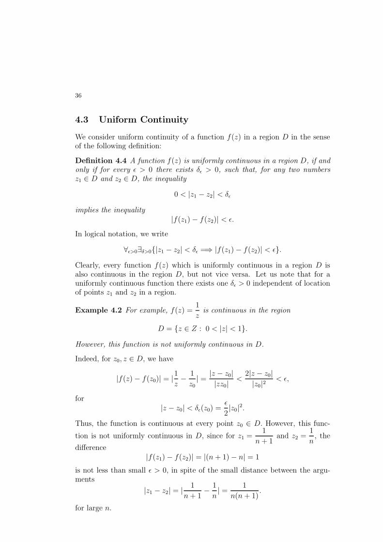
4.3 Uniform Continuity

We consider uniform continuity of a function f(z) in a region D in the senseof the following definition:

Definition 4.4 A function f(z) is uniformly continuous in a region D, if andonly if for every ǫ > 0 there exists δǫ > 0, such that, for any two numbersz1 ∈ D and z2 ∈ D, the inequality

0 < |z1 − z2| < δǫ

implies the inequality|f(z1) − f(z2)| < ǫ.

In logical notation, we write

∀ǫ>0∃δ>0|z1 − z2| < δǫ =⇒ |f(z1) − f(z2)| < ǫ.

Clearly, every function f(z) which is uniformly continuous in a region D isalso continuous in the region D, but not vice versa. Let us note that for auniformly continuous function there exists one δǫ > 0 independent of locationof points z1 and z2 in a region.

Example 4.2 For example, f(z) =1

zis continuous in the region

D = z ∈ Z : 0 < |z| < 1.

However, this function is not uniformly continuous in D.

Indeed, for z0, z ∈ D, we have

|f(z) − f(z0)| = |1z− 1

z0| =

|z − z0||zz0|

<2|z − z0||z0|2

< ǫ,

for|z − z0| < δǫ(z0) =

ǫ

2|z0|2.

Thus, the function is continuous at every point z0 ∈ D. However, this func-

tion is not uniformly continuous in D, since for z1 =1

n + 1and z2 =

1

n, the

difference|f(z1) − f(z2)| = |(n + 1) − n| = 1

is not less than small ǫ > 0, in spite of the small distance between the argu-ments

|z1 − z2| = | 1

n + 1− 1

n| =

1

n(n + 1).

for large n.

37

4.4 Derivatives

Let f(z) be a single valued function defined in a neighborhood of a complexnumber z0. Then, the derivative of f(z) at z0 is defined as the limit

limz→z0

f(z) − f(z0)

z − z0(4.1)

provided that this limit exists, independently of a path, how z approaches z0.If the limit exists then f(z) is said to be differentiable at z0, and its derivative

is denoted by f′(z0) or

df(z0)

dx, otherwise, it is referred to as not differentiable

function.Clearly, we can write the limit (4.1) in the equivalent form

lim∆z→0

f(z0 + ∆z) − f(z0)

∆z

where ∆z = z − z0.

Example 4.3 Let us consider the function

f(z) =√

1 + z, at z0 = i.

Following the definition, we compute

limz→i

√1 + z −

√1 + i

z − i= lim

z→i

z − i

(z − i)√

1 + z +√

1 + i=

1

2√

1 + i=

14√

32e−i

π

8 .

Hence, we have

df(z)

dz |z=i=

d√

1 + z

dz |z=i=

14√

32e−i

π

8 .

One can find a derivative of a function f(z) at a point z0 in Mathematica asthe limit of the Newton’s quotient

Limit[f [z] − f [z0]

z − z0

, z− > z0].

For example, let f(z) =√

1 + z. Then, the command

Limit[(Sqrt[1+z]-Sqrt[1+I])/(z-I), z->I]

gives the derivative (1

4− I

4)√

1 + I =1

4√

32e−i

π

8 .

All rules for derivatives known for real functions are also applicable to complexvariable functions.

38

• Derivatives of some elementary functions. Using the definition ofa derivative, one can find the following formulae:

dzn

dz= nzn−1,

dez

dz= ez,

d sin z

dz= cos z,

d cos z

dz= − sin z,

dtan z

dz=

1

cos2 z,

dcot z

dz= − 1

sin2 z,d ln z

dz=

1

z,

daz

dz= azln a.

• Arithmetic operations on derivatives. Let f(z) and g(z) be differen-tiable functions in a region D. Then the functions f(z)± g(z), f(z)g(z)

andf(z)

g(z)are also differentiable in D and their derivative are given by the

formulae

d(f(z) ± g(z)

dz=

df(z)

dz± dg(z)

dz,

df(z)g(z)

dz= g(z)

df(z)

dz+ f(z)

dg(z)

dz,

d

dzf(z)

g(z) =

f′(z)g(z) − f(z)g

′(z)

g2(z), g(z) 6= 0.

• The derivative of a composed function. Let g(z) be a differentiablefunction at z and f(w) be a differentiable function at w = g(z). Then,the composed function f(g(z)) is differentiable at z and its derivative isgiven by the formula

df(g(z))

dz=

df(w)

dw

dg(z)

dz, w = g(z).

• The derivative of an inverse function. Let w = f(z) be a continuousfunction in a neighbourhood of a point z0 which maps one to one theneighbourhood of z0 into neighbourhood of w0 = f(z0) . If there exits thederivative f

′(z0) 6= 0 then the inverse function z = f−1(w) has derivative

at w0 given by the formula

f (−1)(w0)′

=1

f ′(z0), w0 = f(z0).

In general, derivatives in Mathematica are given by the following commands:

D[f[z],z]; D[f[z],z,n; Dt[f[z[t]],t];

39

where D[f[z],z] stands for the first derivative, D[f[z],z,n] stands for thederivative of order n, and D[f[z[t]],t] stands for the total derivative.For example, let f(z) =

√1 + z. Then, the commands

f[z_]:=Sqrt[1+z];

D[f[z],z]

give the derivative1

2√

1 + z, and the commands

f[z_]:=Sqrt[1+z];

D[f[z],z,2]

give the derivative − 1

4√

1 + z3/2

, and the commands

f[z_]:=Sqrt[1+z];

z[t_]:=2(Cos[t]+I Sin[t]);

D[f[z],z]

give the total derivative

I cos[t] + sin[t]√

1 + 2(cos[t] + I sin[t])

,

4.5 Exercises

Question 4.1 Use the definition to show that

1. (a) the function

f(z) =z2 + 4

z3 − 2z2 + 4z − 8

has the limit g =−1 + i

4, at z0 = −2i.

(b) the function

f(z) =z

z

does have a limit at z0 = 0.

Question 4.2 Let f(z) = 3z2 + 2z. Use the definition to show that

limz→z0

f(z) − f(z0)

z − z0= 6z0 + 2,

at any point z0

Question 4.3 Find the limit

40

1. (a)lim

z→1−i[x + i(2x + y)].

(b)

limz→π

2

sin z

z, Anw :

2

π

(c)

limz→ iπ

2

z2 cosh4z

3, Anw :

π2

8

Question 4.4 Use the definition to show that the function

f(z) = z4 + z2 + 1

is uniformly continuous in the disc |z| ≤ R.

Question 4.5 Show that the function

f(z) =1

z2

is not uniformly continuous in the disc |z| ≤ R, but it is uniformly continuous

in the annulusR

2≤ |z| ≤ R.

Question 4.6 Use the definition of a derivative to show that the functionsf(z) = z − 2, Re z and g(z) = Im z are nowhere differentiable.

Question 4.7 Show that the function f(z) = |z|2 is differentiable at z0 = 0,but it is not differentiable at any point z0 6= 0.

Question 4.8 Let

f(z) =

sin z

z, z 6= 0,

0, z = 0

Show that the function f(z) is differentiable on whole complex plane.

Question 4.9 Let f(z) = u(x, y) + iv)x, y) has derivative f ′(z). Show thatthe function g(z) = u(x, y)− iv(x, y) has derivative g′(z) if and only f ′(z) = 0.

Chapter 5

Analytic Functions

5.1 Cauchy Riemann Equations

Let us consider a complex variable function in the following form:

f(z) = u(x, y) + iv(x, y), z = x + iy.

Suppose that f(z) is differentiable function, that is, there exists limit

lim∆z→0

f(z0 + ∆z) − f(z0)

∆z= f

′

(z), ∆ z = z − z0,

and it is independent on a path through which z approaches z0, (∆ z → 0)Choosing the path along the x axis, we compute

lim∆z→0

f(z0 + ∆z) − f(z0)

∆z= lim

∆x→0

u(x0 + ∆x, y0) − u(x0, y0)

∆x

+i lim∆x→0

v(x0 + ∆x, y0) − v(x0, y0)

∆x

=∂u(x0, y0)

∂x+ i

∂v(x0, y0)

∂x.

Similarly, choosing the path along y axis, we compute

lim∆z→0

f(z0 + ∆z) − f(z0)

∆z= lim

∆y→0

u(x0, y0 + ∆y) − u(x0, y0)

i∆y

+i lim∆y→0

v(x0, x, y0 + ∆y) − v(x0, y0)

i∆y

= −i∂u(x0, y0)

∂y+

∂v(x0, y0)

∂y.

Comparing the right hand sides

∂u(x0, y0)

∂x+ i

∂v(x0, y0)

∂x= −i

∂u(x0, y0)

∂y+

∂v(x0, y0)

∂y.

41

42

we arrive at the Cauchy-Riemann equations

∂u

∂x=

∂v

∂y,

∂u

∂y= −∂v

∂x.

(5.1)

Example 5.1 The exponential function ez, z = x + iy, satisfies Cauchy-Riemannequations, since

ez = ex(cos y + i sin y) = u(x, y) + iv(x, y),

whereu(x, y) = ex cos y, v(x, y) = ex sin y.

Clearly, we have∂u

∂x= ex cos y =

∂v

∂y

∂u

∂y= −ex sin y = −∂v

∂x

In this way, we have proved the following theorem

Theorem 5.1 If a function

f(z) = u(x, y) + iv(x, y), z = x + iy,

possesses derivative f′(z), then functions u(x, y) and v(x, y) satisfy Cauchy-

Riemann equations.

However, there are complex variable functions which satisfy Cauchy-Riemannequations and are not differentiable.

Example 5.2 The function

f(z) =√

|xy| + i xy = u(x, y) + iv(x, y),

satisfies Cauchy-Riemann equations at z = 0, since

∂u(x, 0)

∂x=

∂v(0, y)

∂y= 0

∂u(0, y)

∂y= −∂v(x, 0)

∂x= 0

However, the derivative of f(z) at z = 0 does not exists.

Indeed, for x = αt and y = βt, we have Newton’s quotient

f(z) − f(0)

z=

√

|xy|x + iy

+ ixy

x + iy= ±

√αβ

α + iβ+ i t

αβ

α + iβ.

43

Thus, the limit

limt→0

(±√

|αβ|α + iβ

+ i tαβ

α + iβ) = ±

√

|αβ|α + iβ

.

This limit depends on a path along which z approaches zero. Because fordifferent α or β the limit attains different values, therefore, the derivativef

′(0) does not exist at z = 0.

The following theorem holds:

Theorem 5.2 If the functions u(x, y) and v(x, y) have continuous partialderivatives

∂u

∂x,

∂u

∂y,

∂v

∂x,

∂v

∂y,

in a neighborhood of a complex number z and if Cauchy-Riemann equationshold at z, then the function f(z) possesses the derivative f

′(z) at z.

Thus, Cauchy-Riemann equations are equivalent to differentiability of f(z) =u(x, y)+iv(x, y), provided that the partial derivative ux(x, y), vx(x, y), uy(x, y)and vy(x, y) are continuous functions.The following module checks whether or not a function f(z) = u(x, y)+iv(x, y)satisfies Cauchy Riemann’s equations:

cauchyRiemann[u_,v_]:=Module[ux,uy,vx,vy ,

ux=D[u,x];

vx=D[v,x];

uy=D[u,y];

vy=D[v,y];

(ux===vy)And(uy===-vx)

]

For example, for f(z) = x2 − y2 +2i xy, input u(x, y) and v(x, y) and activatethe module by the commands

u=x^2-y^2;

v=2 x y;

cauchyRiemann[u,v]

to obtain the output True.

5.2 Definition of Analytic Functions

The class of analytic functions is determined by the following definition:

Definition 5.1 .

• A function f(z) is said to be analytic at a complex number z if f(z)possesses the derivative f ′(z) at z and in a neighborhood of z.

44

• A function f(z) is analytic in a domain D if it is analytic at each complexnumber of D.

• A function f(z) is analytic in z = ∞ if f(1

z) is analytic at z = 0.

Later on, we shall show that if an analytic function f(z) possesses its firstderivative then f(z) possesses all derivatives, that is, any analytic function isinfinite times differentiable.In the class of analytic functions, there are two important of subclasses

• Entire functions.

• Harmonic functions.

These subclasses are defined as follows:

Definition 5.2 f(z) is called entire function if it is analytic in whole complexplane.

Definition 5.3 f(z) = u(x, y)+ iv(x, y) is called harmonic function if its realpart u(x, y) and imaginary part v(x, y) are harmonic functions, that is, if theysatisfy Laplace’s equations

∂2u

∂x2+

∂2u

∂y2= 0,

∂2v

∂x2+

∂2v

∂y2= 0.

Now, let us show that real part u(x, y) and imaginary part v(x, y) of an ana-lytic function f(z) = u(x, y) + iv(x, y) are harmonic functions. Indeed, thesefunctions satisfy Cauchy-Riemann equations

∂u(x, y)

∂x=

∂v(x, y)

∂y,

∂u(x, y)

∂y= −∂v(x, y)

∂x.

By differentiation of the first equation with respect to x, and the second equa-tion with respect to y, we get

∂2u(x, y)

∂x2=

∂2v(x, y)

∂x∂y

∂2u(x, y)

∂y2= −∂2v(x, y)

∂y∂x

45

Hence, we have∂2u(x, y)

∂x2+

∂2u(x, y)

∂y2= 0.

Let us note that if f(z) is an analytic function then the derivative

df

dz=

∂f

∂x=

∂u

∂x+ i

∂v

∂x

and alsodf

dz= −i

∂f

∂y= −i

∂u

∂y+

∂v

∂y.

Thus, any analytic function satisfies the following partial differential equation:

∂f

∂x= −i

∂f

∂y, (5.2)

which implies the real Cauchy-Riemann equations. Let f(x, y) be a complexvalued function of two real variables x and y. Clearly, for a complex number

z = x+ iy, we have x =1

2(z + z) and y =

1

2i(z − z). So that, we can consider

f(x(z, z), y(z, z)) as a function of two variables z and z. Applying the rule ofdifferentiation of a composed function, we compute

∂f

∂z=

1

2(∂f

∂x− i

∂f

∂y),

∂f

∂z=

1

2(∂f

∂x+ i

∂f

∂y).

Hence, by equation (5.2), we obtain the following necessary condition to bethe function f analytic

∂f

∂z= 0.

This means an analytic function is independent of z.The following module checks the necessary condition of anslysity of a functionf(z) = u(x, y) + iv(x, y),

analyticCondition[u_,v_]:=Module[z,s,f ,pu,pv,

pu=u[(z+s)/2,(z-s)/(2*I)];

pv=v[(z+s)/2,(z-s)/(2*I)];

f=pu+I*pv;

Simplify[D[f,s]]===0

]

For example, let f(z) = z2. Then, input data functions

u[x_,y_]:=x^2-y^2; v[x_,y_]:=2*x*y;

and execute the module

analyticCondition[u,v]

to obtain the answer True.

46

5.3 Liouville’s Theorem

Let us state Liouville’s theorem for entire functions.

Theorem 5.3 If f(z) is an entire function bounded on the complex plane, thatis, there exists a generic constant M such that

|f(z)| ≤ M, z ∈ Z,

then f(z) is a constant function throughout the whole complex plane.

Proof. f(z) as an entire function satisfies Cauchy’s inequality

|f (n)(z)| ≤ n!M

Rn, n = 0, 1, ...,

for |z| ≤ R and any radius R, where M is a constant independent of R.For n = 1, we have

|f ′(z)| ≤ M

R.

Hence, when R → ∞, we get f ′(z) ≡ 0 for z ∈ Z. This means that f(z) =constant on the whole complex plane.As an implication of Liouville’s theorem, we shall prove the Fundamental The-orem of Algebra.

5.4 Fundamental Theorem of Algebra

Theorem 5.4 Every polynomial

Pn(z) = a0 + a1z + a2z2 + · · ·+ anzn,

of degree n ≥ 1 has at least one zero on complex plane.

Proof. Proving by contradiction, suppose that Pn(z) 6= 0 for all z on thecomplex plane Z. This means that the function

f(z) =1

Pn(z),

is analytic on the whole complex plane, that is, f(z) is an entire function.Now, let us show that f(z) is a bounded function on the whole complex plane.Namely, we have

1

|z|n |a0 + a1z + a2z2 + · · ·+ an−1z

n−1| ≤ |a0||z|n +

|a1||z|n−1

+ · · ·+ |an−1||z| ≤ |an|

2

and

|a0 + a1z + · · ·+ an−1zn−1| ≤ |an| |z|n

2

47

for all |z| ≥ R and sufficiently large R.To estimate f(z), we write

|f(z)| =1

|Pn(z)| ≤1

|an| |z|n − |a0 + a1z + · · ·+ an−1|zn−1| ≤2

|an| |z|n≤ 2

|an| Rn

for all |z| ≥ R.

Thus, f(z) is a bounded by2

|an| |Rnin the region |z| ≥ R and as an analytic

function is also bounded by a constant MR in the disc |z| ≤ R. Thus, f(z) isbounded by the total constant

M = maxMR,2

|an| |R|n,

so that|f(z)| ≤ M, for all z ∈ Z.

By Liouville’s theorem, f(z) is a constant function. This contradicts the as-

sumption Pn(z) 6= 0 for all z ∈ Z. Thus,1

Pn(z)is not an entire function and

Pn(z) has at least one zero on complex plane. The end of the proof.

5.5 Maximum Modulus Principle

If f(z) = u(x, y)+ iv(x, y) is an analytic function inside and on a closed curveC then the maximum value of |f(z)| is attainable at a point z0 ∈ C, that is

maxz∈D∪∈C

|f(z)| = |f(z0)|,

for a certaint point z0 ∈ C.Proof. Let

M(x, y) = |f(z)|2 = u2(x, y) + v2(x, y), z = x + iy,

be the square of the modulus of f(z). We shall show that function M(x, y)satisfies the differential inequality

∂2M(x, y)

∂x2+

∂2M(x, y)

∂y2≥ 0, (5.3)

in the region D enclosed by the curve C. Indeed, we have

∂2M

∂x2+

∂2M

∂y2= 2[

(

∂u

∂x

)2

+

(

∂u

∂y

)2

+

(

∂v

∂x

)2

+

(

∂v

∂y

)2

] ≥ 0.

From the inequality (5.3) it follows that M(x, y) does not attains its maximuminside of C unless it is an constant function.End of the proof.

48

5.6 Exercises

Question 5.1 .

1. (a) Find Cauchy-Riemann equations of an analytic function f(z) = u(x, y)+iv(x, y) in the polar coordinates

x = r cos θ, y = r sin θ, z = x + iy 6= 0.

(b) Check whether or not the function f(z) = z ez satisfies Cauchy-Riemannequations in polar coordinates.

Question 5.2 Show that a harmonic function u satisfies the following formaldifferential equation

∂2u

∂z∂z= 0.

Question 5.3 Determine the coefficients a, b, c and d, to be

1. (a) the quadratic polynomial

ax2 + bxy + cy2

an entier function.

(b) the cubic polynomial

ax3 + bx2y + cxy2 + dy3

an entier function.

Question 5.4 Check weather or not the following functions are entire andsatisfy the Cauchy-Riemann equations:

1. (a)f(z) = xy2 + ix2

(b)f(z) = eyeix.

Question 5.5 Let f(z) be an anslytic function in a region D. Show that iff(z) is real valued function in D then f(z) = constant in the region D.

Question 5.6 Show that the following functions are entire:

1. (a)f(z) = e−yeix, z = x + iy,

(b)f(z) = (z2 − 2)e−xe−iy, z = x + iy.

49

Question 5.7 Let f(z) = u(r, θ) + iv(r, θ), z = r(cos θ + i sin θ) ∈ D beanalytic function in a domain D which does not include number z = 0. UsingCauchy-Riemann equations in polar coordinates, show that function u(r, θ)satisfies Laplace’s equation in polar coordinates equation

r2∂2u

∂r2+ r

∂u

∂r+

∂2u

∂θ2= 0.

Also, show that function v(r, θ) satisfies Laplace’s equation in polar coordi-nates.

Question 5.8 Consider the following function

f(z) = z ez, z = x + iy.

Show that the real part u(x, y) = Re f(z) and the imaginary part v(x, y) =Im f(z) satisfy the following equations:

∂2u

∂z∂z= 0,

∂2v

∂z∂z= 0.

Question 5.9 Consider the following function

f(z) = x2 − y2 + 2ixy, z = x + iy.

Show that this function is analytic and satisfies the equation

∂f

∂z= 0.

Question 5.10 Following details of the proof of fundamental theorem of alge-bra, show that the particular polynomial

P4(z) = z4 − z2 − 2z + 2

has exactly four roots. Determine the roots.

Question 5.11 Find the maximum of |f(z)| in the disc |z| ≤ 1, when f(z) =z4 + z2 + 1.

Question 5.12 Show that for every polynomial

Pn(z) = a0 + a1z + a2z2 + · · · + anzn, an 6= 0, n ≥ 1,

there exists a number R > 0 such that

|Pn(z)| >|an| |z|n

2,

for every |z| > R.

Question 5.13 Show that every harmonic function in a domain D is eitherconstant or does not attain its positive maximum or negative minimum in D.

50

Chapter 6

Integrals

6.1 The Integral of a Complex Valued Function of a

Real Variable

Let us consider the following complex valued function:

w(t) = u(t) + iv(t),

in real the variable t ∈ [α, β].Assuming that the real functions u(t) and v(t) are integrable in the interval[α, β], we define the integral of the complex valued function w(t) by the formula

∫ β

αw(t)dt =

∫ β

αu(t)dt + i

∫ β

αv(t)dt.

Example 6.1 Let w(t) = cos t + i sin t, 0 ≤ t ≤ π

2.

We have∫ π

2

0w(t)dt =

∫ π2

0cos t dt + i

∫ π2

0sin t dt = 1 + i.

The following inequality holds:

|∫ β

αw(t)dt| ≤

∫ β

α|w(t)|dt (6.1)

Indeed, if∫ β

αw(t)dt = 0

then inequality is true.If

∫ β

αw(t)dt 6= 0

then there exist real r0 6= 0 and θ0 such that∫ β

αw(t)dt = r0e

iθ0 .

51

52

Hence, we have

r0 =∫ β

αe−iθ0w(t)dt

and

r0 =∫ β

αRe[e−iθ0w(t)]dt

ButRe[e−iθ0w(t)] ≤ |e−iθ0w(t)| = |w(t)|.

Thus

|∫ β

0w(t)dt| ≤

∫ β

α|w(t)|dt.

One can integrate a complex valued function g(t) of real variable t by thefollowing Mathematica command:

Integrate[g[t],t,a,b]

For example, executing the commands

g[t_]:=t^2+I*Sin[Pi t];

Integrate[g[t],t,0,1]

we obtain the value of the integral

1

3+

2I

π.

6.2 Line Integrals

Let f(z) be a function of complex variable z = x + iy defined on a contour Cgiven by the parametric equation

C : z(t) = x(t) + iy(t), α ≤ t ≤ β.

The line integral of f(z) along the contour C is defined as

∫

Cf(z)dz =

∫ β

αf(z(t))z

′

(t)dt. (6.2)

If f(z) = u(x, y) + iv(x, y), z′(t) = x′(t) + iy′(t) then the line integral takesthe following form:

∫

Cf(z)dz =

∫ β

α(ux′ − vy′)dt + i

∫ β

α(vx′ + uy′)dt.

In terms of differentials dx = x′dt and dy = y′dt, this integral is

∫

Cf(z)dz =

∫ β

α(udx − vdy) + i

∫ β

α(vdx + udy).

53

Example 6.2 Compute the line integral∫

C

dz

z − z0,

along the circle C : z(t) = z0 + Reit, 0 ≤ t < 2π.

We have

f(z) =1

z − z0, z′(t) = iReit,

By formula (6.2), we compute

∫

C

dz

z − z0=

∫ 2π

0

Rieit

Reitdt

=∫ 2π

0idt = 2π i.

Example 6.3 Let us consider the line integral

N(C, a) =1

2πi

∫

C

dz

z − a,

along a closed contour C : z = z(t) α ≤ t ≤ β, . Then, N(C, a) is an integernumber.

Let us note that

N(C, a) =1

2πi

∫ β

α

z′(t) dt

z(t) − a.

We shall show that N(C, a) is an integer number which depends on allocationof a with respect to the curve C.Indeed, the function

g(t) =∫ t

α

z′(s)

z(s) − ads,

has the derivative

g′

(t) =z′(t)

z(t) − a.

Thus, the function

G(t) = e−g(t)[z(t) − a], α ≤ t ≤ β.

has the derivative

dG(t)

dt=

d

dt[e−g(t)(z(t) − a)] = 0, α ≤ t ≤ β.

and G(t) = constant in the interval [α, β]. Because g(α) = 0, therefore

e−g(t)[z(t) − a] = z(α) − a.

54

Hence, we find

eg(t) =z(t) − a

z(α) − a.

and

eg(β) = 1, α ≤ t ≤ β,

when z(β) = z(α).By the theorem 3.1, we obtain g(β) = 2π i N. Thus, we find

N(C, a) =g(β)

2π i= N.

for an integer N .The number N(C, a) is called index of the point a with respect to the curve C.This index indicates how many times point z(t) passes around a when t movesfrom α to β. For example. if C is the circle z(t) = a + Reit, 0 ≤ t ≤ 2π,then N(C, a) = 1, since then point z(t) moves once around the center a whent changes from 0 to 2π.In order to evaluate a contour integral along a piecewise linear path withvertices z1, z2, ..., zm, in Mathenatica, we execute the command

Integrate[g[z], z, z1, z2, ..., zm]

For example, executing the commands

g[z_]:=z*Exp[z^2];

Integrate[g[z],z,0,I,1+I]

we obtain the value of the integral

−1

2+

1

2E2I .

Properties of Line Integrals.

1. (a) From definition of the line integral the following additive propertiescan be easily established:

i.∫

C(f(z) ± g(z))dz =

∫

Cf(z)dz ±

∫

Cg(z)dz.

ii.∫

C(f(z)dz =

∫

C1

f(z)dz +∫

C2

f(z)dz.

where the contour C consists of a contour C1 from z1 to z2 fol-lowed by a contour C2 from z2 to z3.

55

(b)∫

−Cf(z)dz = −

∫

Cf(z)dz.

where the contour C has positive orientation, that is, if t moves fromα to β then z(t) = x(t) + iy(t) moves from z1 = z(α) + iy(α) toz2 = z(β) + iy(β), and the contour −C has opposite orientation toC.Indeed, the parametric equation of the contour −C is

z(−t) = x(−t) + iy(−t), −β ≤ t ≤ −α.

Then, by the substitution s = −t, we have

∫ −α

−βf(z(−t))z′(−t)dt = −

∫ β

αf(z(s))z′(s)ds = −

∫

Cf(z)dz.

(c)

|∫

Cf(z)dz| ≤

∫

C|f(z)|dz

By definition (6.2) and inequality (6.1), we have

|∫

Cf(z)dz| = |

∫ β

αf(z(t))z′(t)dt| ≤

∫ β

α|f(z(t))z′(t)|dt =

∫

C|f(z)|dz

(d) Let |f(z)| ≤ M be bounded function on contour C. Then

|∫

Cf(z)dz| ≤ ML,

where L is the length of C.Since, we have

|∫

Cf(z)dz| ≤ |

∫ β

αf(z(t))z′(t)|dt| ≤ M

∫ β

α|z′(t)|dt ≤ ML.

6.3 Antiderivative

Let f(z) be a function given in the domain D. Every differentiable functionF (z) in domain D which satisfies the condition F ′(z) = f(z), z ∈ D, is calledantiderivative of function f(z). Let us note that the antiderivative F (z) is notuniquely determined since if F (z) is an antiderivative then F (z) + constant isalso an antiderivative of f(z).The following theorem holds:

Theorem 6.1 Let f(z) be a continuous function throughout a domain D andlet F (z) be antiderivative to f(z), that is,

F ′(z) = f(z), z ∈ D.

56

Suppose that a contour C : z(t) = x(t)+ iy(t), α ≤ t ≤ β with the end pointsa = z(α) and b = z(β) lies within the domain D. Then, the line integral isindependent of the path C and its value is given by the formula

∫

Cf(z)dz =

∫ b

af(z)dz = F (b) − F (a).

Proof. Let us the define function Φ(t) = F (z(t)), α ≤ t ≤ β. This functionis differentiable and the derivative

Φ′(t) = f(z(t))z′(t), α ≤ t ≤ β.

Applying the formula (6.2), we obtain the formula

∫

Cf(z)dz =

∫ β

αf(z(t))z′(t)dt =

∫ β

αΦ′(t)dt = Φ(β) − Φ(α) = F (b) − F (a).

Example 6.4 The function f(z) = (z − z0)n has the antiderivative

F (z) =(z − z0)

n+1

n + 1, n 6= −1.

By the thesis of the theorem

∫

C(z − z0)

ndz =1

n + 1[(b − z0)

n+1 − (a − z0)n+1], n 6= −1,

In particular, if the contour C is close, that is, when a = b, the integral∫

C(z − z0)

ndz = 0, n 6= −1,

6.4 Cauchy Theorem

Now, let us state Cauchy theorem.

Theorem 6.2 If f(z) is an analytic function within and on a closed contourC, then

∫

Cf(z)dz = 0.

Example 6.5 If C is the circle |z| = 1 then the integral

∫

C

dz

z2 + 2z + 2= 0.

Since then the singular points z1 = −1 − i and z2 = −1 + i of the integrand

f(z) =1

z2 + 2z + 2=

i

2[

1

z + 1 + i− 1

z + 1 − i]

57

are outside of the circle. Therefore, by Cauchy theorem, the integral along Cis equal to zero.If C0 is the circle |z+1−i| = 1, then the f(z) is not an analytic function in thedisc D = z ∈ Z : |z + 1 − i| ≤ 1. Then, Cauchy theorem is not applicablein D. However, we can compute the integral (see (6.2))

∫

C0

dz

z2 + 2z + 2=∫

C0

i

2[

1

z + 1 + i− 1

z + 1 − i]dz = π.

Let us note, that Cauchy theorem can be confirmed in Mathematica to showthat the integral of an analytic function f(z) along a closed contour C is equalto zero. For example, executing the commands

g[z_]:=z*Exp[z^2];

Integrate[g[z],z,0,I,1+I,0]

we obtain the value of the integral equal to zero.

6.5 Cauchy Integral Formula

Let f(z) be an analytic function within and on a closed contour C which ispositively oriented, that is, oriented in counterclockwise direction.Then the following Cauchy Integral Formula holds:

f(z) =1

2πi

∫

C

f(ζ)

ζ − zdζ, (6.3)

for any z interior to C.Proof. Let z be a complex number interior to C and let Cr be the circle withthe center at z and radius r which is inside of C and has positive orientation.Then, the function

f(ζ)

ζ − z, ζ ∈ C ∪ Cr,

is analytic in the domain D bounded by contour C and circle Cr. Therefore,by Cauchy theorem

∫

C∪Cr

f(ζ)

ζ − zdζ = 0.

Hence, we have∫

C

f(ζ)

ζ − zdζ −

∫

Cr

f(ζ)

ζ − zdζ = 0.

58

-

6'

&

$

%r

Dr

C

Cr

x

y

0

z = x + iy

Fig. 6.1 Domain D

Thus, the integral along curve C is equal to the integral along the circle Cr,that is,

∫

C

f(ζ

ζ − zdζ =

∫

Cr

f(ζ)

ζ − zdζ.

Using the equality∫

Cr

f(ζ)

ζ − zdζ =

∫

Cr

f(z)

ζ − zdζ +

∫

Cr

f(ζ) − f(z)

ζ − zdζ. (6.4)

we obtain∫

Cr

f(z)

ζ − zdζ = 2πif(z), z ∈ D. (6.5)

Because f(z) is an analytic function, therefore for every ǫ > 0 there existsr > 0 such that

|f(ζ)− f(z)| <ǫ

2π, if |ζ − z| < r.

Hence, we get the following ǫ−estimate of the integral

|∫

Cr

f(ζ) − f(z)

ζ − zdζ | ≤ ǫ

2π|∫

Cr

dζ

ζ − z| < ǫ, (6.6)

provided that |ζ − z| < r.Combining equalities (6.4) and the inequality (6.6), we obtain the Cauchy In-tegral Formula.

Example 6.6 Let us evaluate the integral∫

C

z

1 + z2dz, C : |z − i

2| = 1

59

using Cauchy Integral Formula.

The integrandz

1 + z2=

z

(z − i)(z + i),

has the singular point z = i within the circle C : |z − i2| = 1. Thus, the func-

tionf(z) =

z

z + i,

is analytic within and on the circle C. By Cauchy Integral Formula

∫

C

ζ dζ

(ζ + i)(ζ − i)=∫

C

f(ζ)

ζ − idζ = 2πif(i) = πi.

Hence, we obtain∫

C

z dz

1 + z2= π i.

6.6 Cauchy Integral Formula

Theorem 6.3 Let f(z) be an analytic function within and on a closed contourC positively oriented, then the following Cauchy formula holds:

f (n)(z) =n!

2πi

∫

C

f(ζ)

(ζ − z)n+1dζ, n = 0, 1, ..., (6.7)

for any complex number z interior to C.

Proof. We shall prove the theorem using principle of mathematical induction.The theorem is true for n = 0, since it is the case of Cauchy Integral Formulawhich has been already proved.Assuming that the formula is true for n = k, we shall show that the formulais also true for n = k + 1. Indeed, by the assumption, we have

f (k)(z) =k!

2πi

∫

C

f(ζ)

(ζ − z)k+1dζ.

Now, let us consider the Newton quotient

f (k)(z + ∆z) − f (k)(z)

∆z=

k!

2πi∆z

∫

Cf(ζ)[

1

(ζ − z − ∆z)k+1− 1

(ζ − z)k+1]dζ

=k!

2πi

∫

Cf(ζ)

(ζ − z)k+1 − (ζ − z − ∆z)k+1

∆z(ζ − z − ∆z)k+1(ζ − z)k+1dζ.

Using the limit

lim∆z→0

(ζ − z)k+1 − (ζ − z − ∆z)k+1

∆z= (k + 1)(ζ − z)k,

60

one can show that

f (k+1)(z) = lim∆z→0

f (k)(z + ∆z) − f (k)(z)

∆z=

(k + 1)!

2πi

∫

C

f(ζ)

(ζ − z)k+2dζ.

As a consequence of this theorem, the following corollary holds:

Corolary 6.1 If a function f(z) possesses first derivative f ′(z) in a domainD, then f(z) possesses all derivatives in D.

Example 6.7 Use Cauchy Integral Formulas to evaluate the integrals

(i)∫

|z−i|=2

dz

z2 + 4, (ii)

∫

|z−i|=2

dz

(z2 + 4)2.

Let us note that we can write the integrals as follows

(i)∫

|z−i|=2

dz

(z + 2i)(z − 2i), (ii)

∫

|z−i|=2

dz

(z + 2i)2)(z − 2i)2.

Choosing f(z) =1

z + 2i, we can write the first integral as

f(z) =1

2πi

∫

|z−i|=2

f(ζ)

ζ − zdζ.

Thus, for z = 2i, we have

f(2i) =1

4i=

1

2πi

∫

|z−i|=2

dζ

(ζ + 2i)(ζ − 2i)=

1

2πi

∫

|z−i|=2

dz

z2 + 4.

Hence, the first integral is

∫

|z−i|=2

dz

z2 + 4=

π

2.

Similarly, choosing f(z) =1

(z + 2i)2, we have

f(z) =1

2πi

∫

|z−i|=2

f(ζ)

ζ − zdζ.

Thus

f(z) =1

(z + 2i)2=

1

2πi

∫

|z−i|=2

dζ

(ζ + 2i)2(ζ − z).

and the derivative

f′

(z) =−2

(z + 2i)3=

1

2πi

∫

|z−i|=2

dζ

(ζ + 2i)2(ζ − z)2.

61

Hence, for z = 2i, we obtain

−i

32=

1

2πi

∫

|z−i|=2

dζ

(ζ + 2i)2(ζ − z)2=∫

|z−i|=2

dζ

(ζ2 + 4)2,

and the second integral

∫

|z−i|=2

dz

(z2 + 4)2=

π

16.

Also, one can evaluate, in Mathematica, a contour integral of a function f(z)which has singular points interior to a closed contour C. For example, execut-ing the following commands:

g[z_]:=z/(z^2+4);

Simplify[Integrate[g[z],z,-1,1,4 I,-1]]

we obtain the value 2π i of the integral∫

C

z

z2 + 4dz,

along the polygon C with vertices −1, 1, 4i,−1, and with the singular pointz1 = 2i interior to C.

6.7 Cauchy Inequality

If f(z) is analytic inside and on the circle C : |z − a| = R then the followingCauchy inequality holds:

|f (n)(a)| ≤ MR n!

Rn, n = 0, 1, ..., (6.8)

where MR = max|z−a|=R |f(z)|.Indeed, by the Cauchy integral formula

f (n)(a) =n!

2πi

∫

C

f(ζ)

(ζ − a)n+1dζ, n = 0, 1, ...,

we obtain the estimate

|f (n)(a)| =n!

2π|∫

C

f(ζ)

(ζ − a)n+1dζ | ≤ n!

2π

MR

Rn+12πR =

MRn!

Rn.

6.8 Morera Theorem

The inverse to Cauchy’s theorem is Morera theorem. This theorem we shallstate and prove below.

62

Theorem 6.4 If f(z) is a continuous function in a domain D, and if theintegral

∫

Cf(z) dz = 0

along any closed curve C in D, then f(z) is an analytic function.

Proof. Let a be a complex number in the domain D. Then, the functiongiven by the formula

F (z) =∫ z

af(ζ dζ, z ∈ D

is independent of a path in D from a to z. Indeed, if C1 and C2 are two pathsfrom a to z, then the curve C = C1 ∪ −C2 is closed, and by the assumption,the integral

∫

C1∪ −C2

f(ζ) dζ =∫

C1

f(ζ) dζ −∫

C2

f(ζ) dζ = 0.

Hence, we obtain∫

C1

f(ζ) dζ =∫

C2

f(ζ) dζ.

Thus, F (z) is an antiderivative of f(z), so that

F ′(z) = f(z), z ∈ D.

This means that F (z) is an analytic function in D and therefore F (z) hasthe second derivative F

′′(z) = f ′(z), z ∈ D. So that, f(z) possesses first

derivative and it is also analytic function in D.

6.9 Exercises

Question 6.1 Show that for any integer m and n the integral

∫ 2π

0eimte−int dt =

2π, m = n,

0, m 6= n

Question 6.2 Evaluate the integral∫

Cz z dz,

along the positively oriented circle |z| = 1.

Question 6.3 Evaluate the integral∫

C(x + y2 + ixy) dz,

63

along the path

C : z(t) = x(t) + iy(t) =

t + 2i, 1 ≤ t ≤ 2,

2 + i(4 − t) 2 < t ≤ 3

Question 6.4 Show that if C is the circle z(t) = z0 + reit, 0 ≤ t < 2π, posi-tively oriented then

∫

Cf(z) dz = ir

∫ 2π

0f(z0 + reit)eit dt,

for any continuous function f(z).

Question 6.5 Let f(z) be an analytic function inside and on the circle C :z(θ) = a + reiθ, 0 ≤ θ ≤ 2π. show that

f (n)(a) =n!

2πrn

∫ 2π

0e−inθf(a + reiθ)dθ,

for n − 0, 1, 2, ..., and for z interior to C.

Question 6.6 Evaluate the integral

∫

C(z +

1

z) dz,

along the path

1. (a)

z(t) = 2 + eit, 0 ≤ t < 2π,

(b)

z(t) = 1 + i + 2eit, 0 ≤ t < 2π,

(c)

z(t) = 3 eit, 0 ≤ t < 2π.

Question 6.7 Evaluate the integral

1. (a)∫

C[x + 3y2 + i(y − 3x2)]dz,

along the path

C : z(t) = x(t) + iy(t) =

(1 + i)t2, 0 ≤ t ≤ 1,

(2 − t2)i + 1 1 < t ≤ 2

64

Question 6.8 Use Cauchy’s theorem to show that the integral∫

Cz sin z2 dz

is independent of a path with end points a = 1 − i and b = 2 + i.Evaluate the integral.

Question 6.9 Consider the following function:

F (z) =∫

C

dζ

ζ − z, C : |z − a| = R,

Show that

F (z) =

2π i, z ∈ D,

0, z /∈ D ∪ C,

where D is the disk |z − a| < R.

Question 6.10 Use Cauchy Integral Formulas to evaluate the integral

1. (a)∫

|z+2i|=2

dz

z2 − z + 1 − i,

(b)∫

|z+2i|=2

dz

(z2 + z + 1 − i)3,

(c)∫

|z−1|=2

z2 dz

(4 − z2),

(d)

∫

C

e−πz

2 dz

z2 + 4, z(t) = 3i + 2eit, 0 ≤ t < 2π.

(e)

∫

C

e−πz

2 dz

(z2 + 4)3, z(t) = 3i + 2eit, 0 ≤ t < 2π.

(f)∫

C

dz

(4z + 1)2, C : |z − i| = 1.

(g)∫

C

sin 4z + cos 2z

(z − 1)(z − 2), C : |z| = 3.

65

Question 6.11 Use Cauchy inequality to obtain an estimate for the deriva-tives of f(z) = sin z.

Question 6.12 Evaluate∫

|z|=5

zf′(z)

f(z)dz,

where f(z) = z2 + z + 1.

66

Chapter 7

Series

7.1 Power Series

Power series about a point z = z0 is an infinite series of the form

a0 + a1(z − z0) + a2(z − z0)2 + · · · + an(z − z0)

n + · · · =∞∑

n=0

an(z − z0)n,

(7.1)where a0, a1, ..., an, ..., are complex valued coefficients.In most cases, we shall consider a power series about z = 0, that is, the series

a0 + a1z + a2z2 + · · · + anzn + · · · =

∞∑

n=0

anzn, (7.2)

Example 7.1 Let us consider the geometric series

1 + z + z2 + · · ·+ zn + · · · =∞∑

n=0

zn, (7.3)

The geometric series is convergent for |z| < 1, and diverges outside of the unitcircle, so that

∞∑

n=0

zn =

1

1 − z, |z| < 1,

diverges, |z| ≥ 1.

Indeed, the partial sum

Sn = 1 + z + z2 + · · ·+ zn =1 − zn+1

1 − z, z 6= 1.

Clearly, we have

limn→∞

zn = 0, and limn→0

Sn =1

1 − z, for |z| < 1.

67

68

For |z| > 1, the geometric series diverges because the necessary condition ofconvergence is not satisfied, that is

limn→0

zn = ∞, |z| > 1.

Also, the geometric series diverges for |z| = 1, since then

zn = cos nθ + i sin nθ

But sin nθ or cos nθ do not tent to zero when n → 0. Thus, the necessarycondition of convergence is not satisfied, too.The following theorem on convergence of power series holds:

Theorem 7.1 If the power series

∞∑

n=0

anzn,

converges at point z = z1, z1 6= 0, then it absolutely converges in the disc|z| < r = |z1|.Also, if the power series diverges at the point z = z1, then it diverges outsideof the circle, that is for |z| > r.

Proof. Let us assume that the series∞∑

n=0

anzn,

is convergent at point z = z1, so that, the number series

∞∑

n=0

anzn1 ,

is convergent. This means that all terms anzn1 , n = 0, 1, ..., are bounded, so

that, there exists a constant M for which

|anzn1 | ≤ M, n = 0, 1, ...,

Let us note that

|anzn| = |anzn1 | |

z

z1

|n ≤ M | z

z1

|n = Mqn,

for q = | z

z1| < 1.

By the comparison test, the series∞∑

n=0

anzn is absolutely convergent within of

the circle |z| = r = |z1|.Now, let the series

∞∑

n=0

anzn,

69

diverges at point z = z1. Then, the inequality |anzn| > |anzn1 |, holds for

|z| > r, n = 0, 1, ...,By the comparison test, again, we conclude that the series

∞∑

n=0

anzn,

is divergent for |z| > r.Radius of Convergence. The radius R of the circle |z| = R is called radiusof convergence of the series

∞∑

n=0

anzn,

if this series converges for |z| < R and diverges for |z| > R.We compute radius of convergence of a power series using the following for-mula:

R =1

λ, λ = lim

n→∞sup

n

n

√

|an|.

The radius R = ∞ if λ = 0, and the radius R = 0 if λ = ∞.Also, one can compute the radius of convergence of a power series using thefollowing limit:

λ = limn→∞

supn

|an+1

an

|.

Example 7.2 To compute the radius of convergence of the power series

∞∑

n=0

zn

3n + 1,

we find

an =1

3n + 1, λ = lim

n→∞

n

√

1

3n + 1=

1

3, R =

1

λ= 3.

Let us note that the series∞∑

n=0

anzn,

and the series of derivatives∞∑

n=1

nanzn−1,

have the same radius of convergence, since then

λ = limn→∞

supn

n

√

|an| = limn→∞

supn

n

√

n|an|.

70

7.2 Taylor Series.

Let f(z) be an analytic function at a complex number z0. Then, the Taylorseries of f(z) about z0 is defined by the formula

∞∑

n=0

f (n)(z0)

n!(z − z0)

n.

In the case when z0 = 0, the Taylor series is called Maclaurin series.The following theorem holds:

Theorem 7.2 If f(z) is an analytic function at z0, then its Taylor seriesconverges and

f(z) =∞∑

n=0

f (n)(z0)

n!(z − z0)

n.

for |z − z0| < R, where R is the radius of the circle within which the functionf(z) is analytic.

Proof. Let f(z) be an analytic function within the circle |z − z0| = R.Then, by Cauchy integral formula, we have

f(z) =1

2πi

∫

|ζ−z0|=R

f(ζ)

ζ − zdζ, z ∈ D = z : |z − z0| < R.

Let us note that

1

ζ − z=

1

(ζ − z0) − (z − z0)

=1

ζ − z0

1

1 − z−z0

ζ−z0

=1

ζ − z0[1 +

z − z0

ζ − z0+ (

z − z0

ζ − z0)2 + · · ·+ (

z − z0

ζ − z0)n + · · ·]

for |ζ − z0| = R.Hence, we obtain

1

ζ − z=

∞∑

n=0

(z − z0)n

(ζ − z0)n+1, |z − z0| < |ζ − z0| < R.

Now, coming back to Cauchy formula, we find

f(z) =1

2πi

∫

|ζ−z0|=R

f(ζ)

ζ − zdζ =

1

2πi

∫

|ζ−z0|=Rf(ζ)

∞∑

n=0

(z − z0)n

(ζ − z0)n+1dζ

=∞∑

n=0

(z − z0)n

n!

n!

2πi

∫

|ζ−z0|=R

f(ζ)

(ζ − z0)n+1dζ

71

Hence, by the formula

f (n)(z0) =n!

2πi

∫

|ζ−z0|=R

f(ζ)

(ζ − z0)n+1dζ,

we obtain the following Taylor series representation of f(z):

f(z) =∞∑

n=0

f (n)(z0)

n!(z − z0)

n,

for |z − z0| < R.

Example 7.3 It is easily to establish Taylor series of the following elementaryfunctions:

1. (a)

ez = 1 +z

1!+

z2

2!+ · · ·+ zn

n!+ · · · , z ∈ Z,

(b)

sin z = z − z3

3!+

z5

5!+ · · ·+ (−1)n+1 z2n−1

(2n − 1)!+ · · · , z ∈ Z,

(c)

cos z = 1 − z2

2!+

z4

4!+ · · ·+ (−1)n z2n

2n!+ · · · , z ∈ Z,

(d)

ln(1 + z) = z − z2

2+

z3

3+ · · ·+ (−1)n+1 zn

n+ · · · , |z| < 1.

Taylor series with n-th terms of a function f(z) about a point a can be obtainedin Mathematica by the command

Series[f[z],z,a,n]

For example, the output of the following commands:

f[z_]:=Sin[z]Exp[z];

Normal[Series[f[z],z,0,6]]

is the series

z +z2

1+

z3

3− z5

30− z6

90.

72

7.3 Laurent Series

Let

D(z0, r1, r2) = z ∈ Z : 0 < r1 < |z − z0| < r2.be the annulus with radii r1 and r2 and the center at the point z0. A Laurentseries is considered in the annulus D(z0, r1, r2). A Laurent series takes thefollowing form:

∞∑

n=1

a−n(z − z0)−n +

∞∑

n=0

an(z − z0)n =

∞∑

n=−∞

an(z − z0)n.

Let us note that a Laurent series consists of the principal part

∞∑

n=1

a−n(z − z0)−n,

and the regular part∞∑

n=0

an(z − z0)n.

A Laurent series is said to be convergent in annulus D(z0, r1, r2) if both seriesin regular part and principal part are convergent, otherwise the Laurent seriesis divergent. Clearly, the series in the regular part is convergent in the disc

|z − z0| < r2, r2 =1

λ, λ = lim

n→∞sup

n

n

√

|an|.

and divergent outside of the disc, that is, for |z − z0| > r2.The series in the principal part is divergent in the disc |z − z0| < r1, andconvergent outside of the disc, that is for |z − z0| > r1. Thus, both parts ofthe Laurent series are convergent in the annulus D(z0, r1, r2).The following theorem holds:

Theorem 7.3 If f(z) is an analytic function in the annulus D(z0, r1, r2), thenthe Laurent series of f(z) is convergent and

f(z) =∞∑

n=−∞

an(z − z0)n, z ∈ D(z0, r1, r2),

where the coefficients

an =1

2πi

∫

C

f(ζ)

(ζ − z0)n+1dζ, n = 0 ± 1,±2, ...,

Proof. Let z be a complex number in the annulus D(z0, r1, r2) which boundaryconsists with two circles C1(z0, r1) and C2(z0, r2). Dividing the annulus in two

73

parts as on figure 8.1, we obtain the domain D1 and D2 with the boundaries∂D1 and ∂D2. By Cauchy Integral formula, we have

f(z) =1

2πi

∫

∂D2

f(ζ)

ζ − zdζ, z ∈ D2,

and1

2πi

∫

∂D1

f(ζ)

ζ − zdζ = 0, z ∈ D2,

Adding both integrals and canceling the integrals along the common parts ofthe boundaries ∂D1 and ∂D2, we obtain the formula

f(z) =1

2πi

∫

C2

f(ζ)

ζ − zdζ − 1

2πi

∫

C1

f(ζ)

ζ − zdζ, z ∈ D(z0, r1, r2). (7.4)

Fig. 8.1 Singular point zLet us note that |ζ − z0| > |z − z0| for ζ ∈ C2, so that

1

ζ − z=

1

(ζ − z0) − (z − z0)

=1

ζ − z0

1

1 − z−z0

ζ−z0

=∞∑

n=0

(ζ − z0)n

(z − z0)n+1,

Also, for |ζ − z0| < |z − z0|, when ζ ∈ C1, we have

1

ζ − z=

1

(ζ − z0) − (z − z0)

= − 1

z − z0

1

1 − ζ−z0

z−z0

= −∞∑

n=1

(ζ − z0)n−1

(z − z0)n.

Both the above series are uniformly convergent with respect to ζ . Therefore,

we can replace the function1

ζ − zin the integrals in (7.4) by these series.

74

Then, we obtain the following formula:

f(z) =∞∑

n=0

1

2πi

∫

C2

f(ζ)

(ζ − z0)n+1dζ (z − z0)

n

+∞∑

n=0

1

2πi

∫

C1

f(ζ)

(ζ − z0)n+1dζ (z − z0)

−n.

(7.5)

We can replace the two integrals in (7.5) along the circles C1 and C2 by theintegral along a circle C within the annulus D(z0, r1, r2). Then, we obtain theLaurent series

f(z) =∞∑

n=0

an(z − z0)n +

∞∑

n=1

a−n(z − z0)−n, z ∈ D(z0, r1, r2),

where the coefficients

an =1

2πi

∫

C

f(ζ)

(ζ − z0)n+1dζ, n = 0,±1,±2, ...,

End of the proof.

Example 7.4 Let us consider the following function:

f(z) =1

z − 2+

1

z − 1.

This function is analytic in the annulus D(0, 1, 2) = z ∈ Z : 1 < |z| < 2.Then

1

z − 2= −1

2

1

1 − z2

= −∞∑

n=0

zn

2n+1, |z| < 2,

and1

z − 1=

1

z

1

1 − 1z

=∞∑

n=1

1

zn, |z| > 1.

Hence, the Laurent series of f(z) is

f(z) =1

z − 2+

1

z − 1= −

∞∑

n=0

zn

2n+1+

∞∑

n=1

1

zn, 1 < |z| < 2.

A Laurent series with n terms of a function f(z) about a point a can be easilyobtained in Mathematica by the command

Series[f[z],z,a,n]

For example, let f(z) =z

z2 + 1, n = 6, a = i. Then, we obtain, in Mathematica,

six terms of the Laurent series by the following commands:

75

f[z_]:=z/(z^2+1);

Normal[Series[f[z],z,I,6]]

−I

4+

1

2(z − I)+

1

8(z − I) +

1

16I(z − I)2

− 1

32(z − I)3 − 1

64I(z − I)4 +

1

128(z − I)5 +

1

256I(z − I)6.

7.4 Exercises

Question 7.1 Find the region of convergence of the series

1. (a)∞∑

n=0

(z + 2)n

(n + 2)34n+1,

(b)∞∑

n=1

(−1)n−1z2n−1

(2n − 1)!.

Question 7.2 Find the region of convergence of the series

1. (a)∞∑

n=1

1

n2 + z2,

(b)∞∑

n=1

cos nz

n3.

Question 7.3 Use the geometric series

z + z2 + · · ·+ zn + · · · =z

1 − z, |z| < 1,

to show the following:

1. (a)∞∑

n=1

rn cos nθ =r cos θ − r2

1 − 2r cos θ + r2,

(b)∞∑

n=1

rn sin nθ =r sin θ − r2

1 − 2r cos θ + r2.

Question 7.4 Find the Taylor series for the following functions about theindicated points

76

1. (a)

f(z) = cos z, z0 =π

2,

(b)g(z) = sinh z, z0 = πi.

Question 7.5 Find the Laurent series for the function

f(z) =1

z2(1 − z),

1. (a) in the annulus0 < |z| < 1,

(b) in the annulus1 < |z| < ∞.

Question 7.6 Find the Laurent series for the function

f(z) =1

z2+

1

1 − z+

1

2 − z,

1. (a) in the annulus0 < |z| < 1,

(b) in the annulus1 < |z| < 2,

(c) in the annulus2 < |z| < ∞.

Question 7.7 Find principal part of the Laurent series for the following func-tions:

1. (a)

f(z) =1

z2 sin z, z0 = 0,

(b)

f(z) =eiz

z2 + 4, z0 = 2i,

(c)

f(z) =z − sin z

z3, |z| > 0.

Chapter 8

Residues

8.1 Singular Points

There are three types of singular points of a function f(z) at a point z0.

1. (a) z0 is a removable singular point of f(z) if the Laurent series of f(z)about z0 reduces to the regular part.

(b) z0 is pole of order m if the principal part of the Laurent series aboutz0 has m terms, that is, · · ·a−m−2 = a−m−1 = 0, and a−m 6= 0.

(c) z0 is essential singular point of f(z) if the principal part of the Laurentseries has infinite number of terms.

Example 8.1 Let us consider the following function:

f(z) =z − i

z2 + 1,

with the singular points z0 = i and z0 = −i.

This function has the following Laurent series about the point z0 = i:

f(z) =1

z + i=

1

(z − i) + 2i=

1

2i

1

1 + z−i2i

=1

2i[1 − z − i

2i+ (

z − i

2i)2 − · · ·+ (−1)n(

z − i

2i)n + · · ·]

=1

2i

∞∑

n=0

(−1)n(z − i

2i)n.

Since the principal part of the Laurent series of f(z) has been reduced to zero(a−1 = a−2 = · · · = a−m = · · · = 0), therefore z0 = i is a removable singularpoint of f(z).

Example 8.2 Let us consider the following function:

f(z) =1

z2 + 1.

77

78

with the singular points z0 = i and z0 = −i.

This function has the following Laurent series about z0 = i:

f(z) =1

z2 + 1=

1

(z − i)(z + i)

=1

2i

1

z − i− 1

2i

1

z + i

=1

2i

1

z − i− 1

2i

1

(z − i) + 2i

=1

2i

1

z − i+

1

4

1

1 +z − i

2i1

2i

1

z − i+

∞∑

n=1

(−1)n (z − i)n−1

(2i)n+1.

The principal part of the series consists of one term and a1 =1

2i. Thus, z0 = i

is the pole of order one.

Example 8.3 let us consider the following function

f(z) = e

1

z .

This function has the following Laurent series about z0 = 0:

e

1

z = 1 +1

1!z+

1

2!z2+ · · ·+ 1

n!zn+ · · ·

Because the principal part of the Laurent series has infinite number of terms,therefore z0 = 0 is the essential singular point of f(z).

8.2 Residues

Let f(z) be an analytic function in the annulus 0 < |z − z0| < r. Then, thecoefficient a−1 in the Laurent series

f(z) =∞∑

n=1

a−n(z − z0)−n +

∞∑

n=0

an(z − z0)n,

is called residue of f(z). In symbols, we write Res f(z) |z0= a−1.

Example 8.4 The function

f(z) =1

z2(z − 3)2=

1

9(z − 3)2− 2

27(z − 3)+

1

27− 4(z − 3)

243+ · · ·

has the pole of order two at z0 = 3 and the residue Res f(z) |z0=3 = a−1 = − 2

27.

79

If f(z) has the Laurent series

f(z) =∞∑

n=1

a−n(z − z0)−n +

∞∑

n=0

an(z − z0)n, (8.1)

then the residue

a−1 = Resf(z)|z0=

1

2πi

∫

Cf(z) dz. (8.2)

Indeed, integrating both sides of (8.1), we obtain

∫

Cf(z) dz =

∞∑

n=1

a−n

∫

C(z − z0)

−n dz +∞∑

n=0

an

∫

C(z − z0)

n dz,

where C is a closed contour within the annulus 0 < |z − z0| < r.

Because(z − z0)

n+1

n + 1is the antiderivative to (z − z0)

n, when n 6= −1, there-

fore, the integrals∫

C(z − z0)

n dz = 0, for n 6= −1.

But, for n = −1, we have∫

C

dz

z − z0

= 2πi.

Hence, we obtain the formula (8.2).

Example 8.5 Compute the residue of the function

f(z) =z

1 + z2,

at the singular points z0 = i and z0 = −i.

Let C(i, 1) : |z − i| = 1, be the circle with radius r = 1 at the center z0 = i.Then, by the formula (8.2), we compute the residue

a−1 = Resz

1 + z2|z0=i =

1

2πi

∫

C

z

1 + z2dz =

1

2

1

2πi

∫

C[

1

z − i+

1

z + i]dz =

1

2.

Also, we compute

a−1 = Resz

1 + z2|z0=−i =

1

2πi

∫

C

z

1 + z2dz =

1

2πi

1

2

∫

C[

1

z − i+

1

z + i]dz =

1

2.

for z0 = −i and C(−i, 1) : |z + i| = 1.If f(z) has a simple singular pole at z0, that is a pole of order one, then theresidue

Res f(z)|z0= lim

z→z0

(z − z0)f(z). (8.3)

80

Indeed, in this case, the Laurent series of f(z) is:

f(z) = a−11

z − z0+ a0 + a1(z − z0) + a2(z − z0)

2 + · · ·

Hence , we obtain

(z − z0)f(z) = a−1 + a0(z − z0) + a1(z − z0)2 + · · ·

andlimz→z0

(z − z0)f(z) = Res f(z) |z0 = a−1.

Example 8.6 The function

f(z) =1 − z2

z(1 + z2),

has simple poles at z = i, z = −i and z = 0.By the formula (8.3), we compute

Res f(z)|z=i = limz→i

(z − i)1 − z2

z(z − i)(z + i)= −1,

Res f(z)|z=−i = limz→−i

(z + i)1 − z2

z(z − i)(z + i)= 1,

Res f(z)|z=0 = limz→0

z1 − z2

z(z − i)(z + i)= 1.

Let us assume that f(z) is an analytic function in a neighborhood of z0, andhas a pole of order m at the point z0. Then, the residue of f(z) at z0 is givenby the formula

Resf(z)|z0= lim

z→z0

Φ(m−1)(z)

(m − 1)!, (8.4)

where the functionΦ(z) = (z − z0)

mf(z)

has a removable singular point at z0.If we define

Φ(z0) = a−m, a−m 6= 0,

then Φ(z) is analytic function also at z0 and has the following series represen-tation

Φ(z) = a−m + a−m+1(z − z0) + · · · + a−1(z − z0)m−1 + a0(z − z0)

m + · · ·Hence, we compute the residue

a−1 = Res f(z)|z0= lim

z→z0

Φ(m−1)(z0)

(m − 1)!.

One can easily obtain a residue in Mathematica by the following command:

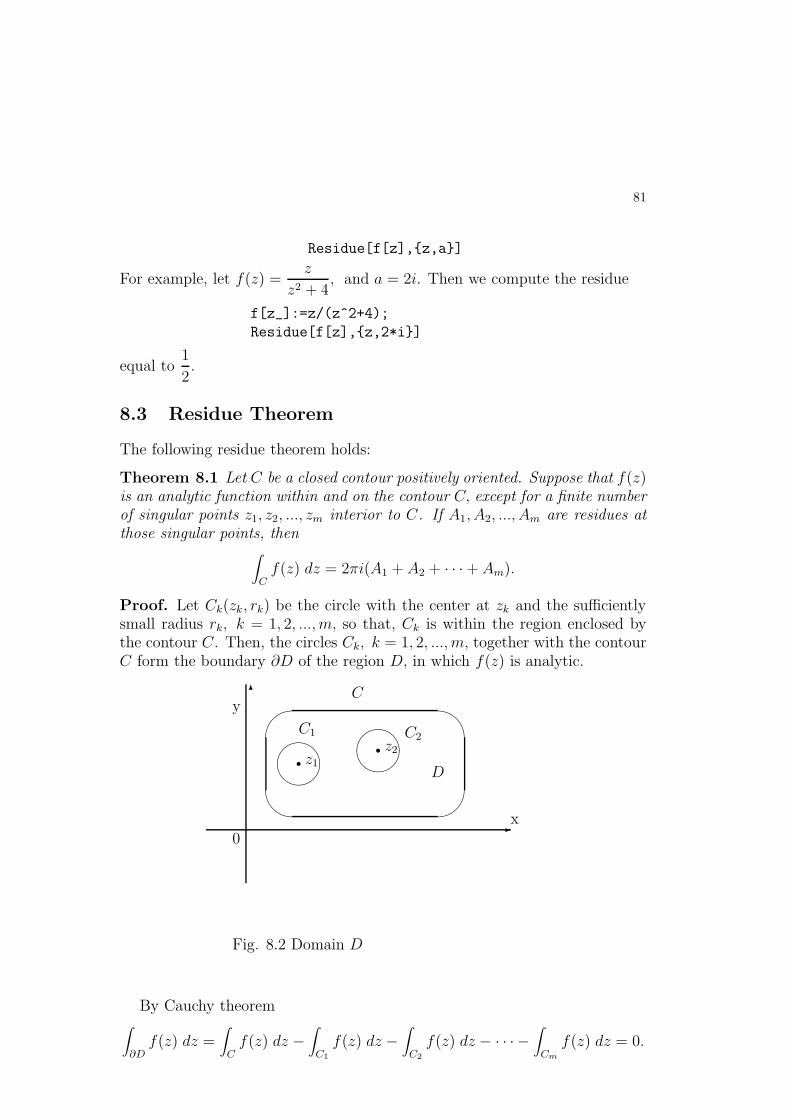
81

Residue[f[z],z,a]

For example, let f(z) =z

z2 + 4, and a = 2i. Then we compute the residue

f[z_]:=z/(z^2+4);

Residue[f[z],z,2*i]

equal to1

2.

8.3 Residue Theorem

The following residue theorem holds:

Theorem 8.1 Let C be a closed contour positively oriented. Suppose that f(z)is an analytic function within and on the contour C, except for a finite numberof singular points z1, z2, ..., zm interior to C. If A1, A2, ..., Am are residues atthose singular points, then

∫

Cf(z) dz = 2πi(A1 + A2 + · · · + Am).

Proof. Let Ck(zk, rk) be the circle with the center at zk and the sufficientlysmall radius rk, k = 1, 2, ..., m, so that, Ck is within the region enclosed bythe contour C. Then, the circles Ck, k = 1, 2, ..., m, together with the contourC form the boundary ∂D of the region D, in which f(z) is analytic.

-

6'

&

$

%r

r z2

C2

D

C

C1

x

y

0

z1

Fig. 8.2 Domain D

By Cauchy theorem∫

∂Df(z) dz =

∫

Cf(z) dz −

∫

C1

f(z) dz −∫

C2

f(z) dz − · · · −∫

Cm

f(z) dz = 0.

82

Because

Ak =1

2πi

∫

Ck

f(z) dz, k = 1, 2, ..., m,

therefore∫

Cf(z) dz = 2πi(A1 + A2 + · · · + Am).

End of proof.

Example 8.7 Let us evaluate the integral

∫

|z|=2

5z − 4

(z + 1)(z − 1)dz.

The integrand has two singular points z = 1 and z = −1 both interior to thecircle C : |z| = 2. The residues are:

Resf(z)|z=1 = limz→1

(z − 1)5z − 4

(z − 1)(z + 1)=

1

2,

Resf(z)|z=−1 = limz→−1

(z + 1)5z − 4

(z − 1)(z + 1)=

9

2.

By the residue theorem

∫

|z|=2

5z − 4

(z + 1)(z − 1)dz = 2πi(

1

2+

9

2) = 10πi.

Example 8.8 Let us evaluate the integral∫

|z|=2

z

z2 + 2z + 2dz,

using Mathematica.

The functionz

z2 + 2z + 2, has two singular points z1 = −1+ i and z2 = −1− i

within the circle |z| = 2. We compute the residues at these points by thefollowing commands:

f[z_]:=z/(z^2+2 z+2);

Residue[f[z],z,-1+I;

Residue[f[z],z,-1-I];

equal to A1 =1

2+

I

2and A2 =

1

2− I

2. By the residue theorem, the integral

∫

|z|=2

z

z2 + 2z + 2dz = 2πi(A1 + A2) = 2πi,

83

8.4 Applications of the Residue Theorem

As an application of the residue theorem, we shall evaluate the following im-proper integral:

∫ ∞

−∞f(x) dx.

The following theorem holds:

Theorem 8.2 Let f(z) be an analytic function in the upper half plane Im z ≥0, except at the singular points z1, z2, ..., zm interior to the upper half of thecomplex plane, at which f(z) has residue A1, A2, ..., Am. If f(z) is a realfunction on the x axis and satisfies the condition

|f(z)| ≤ M

|R|α , |z| ≥ R,

for certain constants M > 0, R > 0 and α > 1, then the infinite integral existsand its value is given by the formula

∫ ∞

−∞f(x) dx = 2πi(A1 + A2 + · · · + Am).

Proof. Let C be the contour consisting with the interval I = [−R, R] and thehalf of the circle Γ : z(t) = Reit, 0 ≤ t ≤ π, that is C = I ∪ Γ,(see Figure8.2). Let us choose R so large to be all singular points interior to the closedcontour C.

Fig. 8.2 ResidueBy residue theorem

∫

Cf(z) dz =

∫ R

−Rf(x) dx +

∫

Γf(z) dz = 2πi

m∑

k=1

Ak.

By the assumptions, we have the following estimate of the integral along Γ:

|∫

Γf(z) dz| ≤ M

RαπR =

πM

Rα−1, α > 1.

84

Clearly, if R → ∞, then the integral along Γ tends to zero, and the firstintegral becomes

∫ ∞

−∞f(x) dx = 2πi

m∑

k=1

Ak.

End of the proof.

Example 8.9 Evaluate the integral

∫ ∞

−∞

dx

1 + x2.

We consider the function

f(z) =1

1 + z2=

1

(z − i)(z + i)

which has one singular point z = i in the upper half of complex plane. By theresidue theorem

∫

C

dx

1 + z2=∫ R

−R

dx

1 + x2+∫

Γ

dz

1 + z2= 2π i Res

1

1 + z2|z=i = π.

The function f(z) satisfies the inequality

|f(z)| =1

|1 + z2| ≤1

|z|2 − 1≤ 1

|z|2 − |z|22

=2

|z|2 ≤ 2

R2for |z| ≥ R ≥ 2.

Therefore, the integral

|∫

Γ

dz

1 + z2| ≤ 1

R2|∫

Γdz| =

π

R.

Hence, when R → ∞, we obtain

∫

Γ

dz

1 + z2= 0,

and∫ ∞

−∞

dx

1 + x2= π.

Example 8.10 Show that

∫ ∞

−∞

dx

ax2 + bx + c=

2π√4ac − b2

, ∆ = b2 − 4ac < 0, a 6= 0. (8.5)

We apply theorem 8.2. Let us consider the function

f(z) =1

az2 + bz + c,

85

with real coefficients a, b and c and the discriminant ∆ = b2 − 4ac < 0, a 6= 0.We shall show that the function f(z) satisfies the assumptions of the theorem.Firstly, we note that f(z) is the real valued function on x-axis, so that, forz = x,

f(x) =1

ax2 + bx + c.

Secondly, the function f(z) satisfies the inequality

|f(z)| ≤ 2

|a|R2, |z| ≥ R,

where R =1

|a| [|b| +√

|b|2 + 2|ac|], M =2

|a| , α = 2.

Indeed, to show the inequality, we estimate

|az2 + bz + c| ≥ |az2| − |bz + c|

|bz + c| ≤ |b||z| + |c| ≤ 1

2|a||z|2,

1

2|a||z|2 − |b||z| − |c| ≥ 0,

The last quadratic inequality holds for |z| ≥ R =1

|a| [|b| +√

|b|2 + 2|ac|].Hence, we obtain the estimate

1

|az2 + bz + c| ≤1

|az2| − |bz + c| ≤2

|a||z|2 ≤ 2

|a|R2.

The function f(z) has one singular point z1 =−b + i

√−∆

2ain the upper half

of complex plane at which

Resf(z)|z=z1

= limz→z1

(z − z1)1

a(z − z1)(z − z1)= − i√

−∆.

By the theorem∫ ∞

−∞

dx

ax2 + bx + c= 2πiResf(z)

|z=z1=

2π√4ac − b2

, a 6= 0.

Example 8.11 Evaluate the integral∫ ∞

−∞

dx

x2 − x + 1

We apply the formula (8.5), when a = 1, b = −1, c = 1, and the discriminant∆ = −3.Thus, we find

∫ ∞

−∞

dx

x2 − x + 1=

2π√3.

86

Example 8.12 Let us evaluate the integral∫ ∞

−∞

dx

(1 + x2)n+1.

Clearly, the function

f(z) =1

(1 + z2)n+1=

1

(z − i)n+1(z + i)n+1.

has a pole of order n + 1 at z0 = i and z0 = −i. Since, z = i is only thesingular point of f(z) in upper half of complex plane, therefore, by the residuetheorem

∫

C

dz

(1 + z2)n+1= 2π i Res f(z)|z=i, (8.6)

where the closed contour C = [−R, R] ∪ Γ.Let us compute the residue using formula (8.6). Clearly, we have m = n + 1and

Φ(z) = (z − i)n+1 1

(1 + z2)n+1=

1

(z + i)n+1.

Because

Res f(z)|i = limz→i

1

n!

dn

dzn

1

(z + i)n+1=

(−1)n

(2i)2n+1

(2n)!

(n!)2,

therefore, the integral∫

C

dz

(1 + z2)n+1=

∫ R

−R

dx

(1 + x2)n+1+∫

Γ

dz

(1 + z2)n+1

= 2π i Res f(z)|z=i =(2n)!

(n!)2

π

4n.

Let us note that the function f(z) satisfies the inequality

|f(z)| =1

|(1 + z2)n+1| ≤2

|z|2n+2≤ 2

R2n+2, |z| ≥ R ≥ 2.

Thus, we get the following estimate of the integral along the curve Γ:

|∫

Γ

dz

1 + z2|n+1 ≤ 2π

R2n+2.

Hence, when R → ∞, we get∫

Γ

dz

(1 + z2)= 0,

and∫ ∞

−∞

dx

(1 + x2)n+1=

(2n)!

(n!)2

π

4n.

87

One can easily compute an improper integral in Mathematica using the fol-lowing command:

Integrate[f[x], x,−∞,∞].For example, we evaluate the integral

∫ ∞

−∞

dx

x2 + 8,

by the command:

Integrate[1

x2 + 8, x,−∞,∞],

to get the valueπ√

2

4.

Example 8.13 Evaluate the integral

∫ ∞

−∞

x sin x

x2 + a2dx, a > 0.

Consider the function

f(z) =zeiz

z2 + a2

The fuction f(z) has one simple singular point z1 = ia, a > 0, in the upperhalf of the complex plane. By the residue theorem

∫ R

−R

xeix

x2 + a2dx + i

∫

Γ

zeiz

z2 + a2dx = 2πiA1, a > 0.

where the residue

A1 = limz−>ia

(z − ia)zeiz

z2 + a2= lim

z−>ia

zeiz

z + ia=

1

2e−a

8.5 Exercises

Question 8.1 Locate and classify the singularities of the following functions:

1. (a)

f(z) =eiz

(z2 + z + 1)2,

(b)

f(z) =z sin z

cos z − 1.

Question 8.2 Find the residues at singular points for the following functions:

88

1. (a)

f(z) =1 + z

z2 − 2z,

(b)

f(z) = (z − 3) sin1

z + 2,

(c)

f(z) =z2 − 2z

(z + 1)2(z2 + 4),

(d)

f(z) =1

sin z,

(e)

f(z) =1

(1 + z4)2,

Question 8.3 Using residue theorem, evaluate the following integrals:

1. (a)∫

|z|=4

3z3 + 2

(z − 1)(z2 + 9)dz,

(b)∫

|z|=1sin

1

zdz,

(c)∫

C

cosh z

z3dz,

where C is the square with vertices ±2 ± 2i. Ans. πi.

Question 8.4 Using residue theorem evaluate the following infinite integrals

1. (a)∫ ∞

−∞

dx

x2 + 2x + 2,

(b)∫ ∞

0

dx

1 + x4,

(c)∫ ∞

0

dx

x4 + x2 + 1,

89

(d)∫ ∞

−∞

x sin x

x2 + a2dx,

(e)∫ ∞

−∞

cos nx

1 + x2dx,

(f)∫ ∞

−∞

dx

(1 + x2)8,

Question 8.5 Use the function f(z) = e−z2

, to evaluate Fresnel’s integrals

1. (a)∫ ∞

0sin x2 dx,

(b)∫ ∞

0cos x2 dx,

Index

analytic functions, 43annulus, 10antiderivative, 55arc, 12

bounded set, 12

Cauchy inequality, 61Cauchy integral formula, 57Cauchy Riemann equations, 41Cauchy’s theorem, 56circle, 9complex numbers, 1conjugate complex number, 2connected set, 12continuity, 35contour, 12

derivatives, 37disc, 10

entire functions, 44exponential function, 19

fundamental theorem of algebra, 46

harmonic functions, 44hyperbolic functions, 24

Laurent series, 72limit, 33line integral, 52line segment, 9linear fractional function, 26linear function, 15Liouville’s theorem, 46logarithm of a complex number, 6logarithmic function, 20

maximum principle, 47Morera theorem, 61

neighborhood, 11

open set, 12

power function, 17power series, 67principal argument, 3

residue, 78residue theorem, 81root function, 18root of z, 4rotation, 16

sector, 11singular point, 77strip, 10

Taylor series, 70translation, 15trigonometric functions, 23

90