lecture notes in computer science 4618
TRANSCRIPT

Lecture Notes in Computer Science 4618Commenced Publication in 1973Founding and Former Series Editors:Gerhard Goos, Juris Hartmanis, and Jan van Leeuwen
Editorial Board
David HutchisonLancaster University, UK
Takeo KanadeCarnegie Mellon University, Pittsburgh, PA, USA
Josef KittlerUniversity of Surrey, Guildford, UK
Jon M. KleinbergCornell University, Ithaca, NY, USA
Friedemann MatternETH Zurich, Switzerland
John C. MitchellStanford University, CA, USA
Moni NaorWeizmann Institute of Science, Rehovot, Israel
Oscar NierstraszUniversity of Bern, Switzerland
C. Pandu RanganIndian Institute of Technology, Madras, India
Bernhard SteffenUniversity of Dortmund, Germany
Madhu SudanMassachusetts Institute of Technology, MA, USA
Demetri TerzopoulosUniversity of California, Los Angeles, CA, USA
Doug TygarUniversity of California, Berkeley, CA, USA
Moshe Y. VardiRice University, Houston, TX, USA
Gerhard WeikumMax-Planck Institute of Computer Science, Saarbruecken, Germany
Please purchase PDF Split-Merge on www.verypdf.com to remove this watermark.
Selim G. Akl Cristian S. CaludeMichael J. Dinneen Grzegorz RozenbergH. Todd Wareham (Eds.)
UnconventionalComputation
6th International Conference, UC 2007Kingston, Canada, August 13-17, 2007Proceedings
13
Please purchase PDF Split-Merge on www.verypdf.com to remove this watermark.

Volume Editors
Selim G. AklQueen’s UniversitySchool of Computing, Kingston, Ontario K7L 3N6, CanadaE-mail: [email protected]
Cristian S. CaludeMichael J. DinneenUniversity of AucklandDepartment of Computer Science, Auckland, New ZealandE-mail: {cristian, mjd}@cs.auckland.ac.nz
Grzegorz RozenbergUniversity of ColoradoDepartment of Computer Science, Boulder, Co 80309-0347, USAE-mail: [email protected]
H. Todd WarehamMemorial University of NewfoundlandDepartment of Computer Science, St. John’s, NL, CanadaE-mail: [email protected]
Library of Congress Control Number: 2007932233
CR Subject Classification (1998): F.1, F.2
LNCS Sublibrary: SL 1 – Theoretical Computer Science and General Issues
ISSN 0302-9743ISBN-10 3-540-73553-4 Springer Berlin Heidelberg New YorkISBN-13 978-3-540-73553-3 Springer Berlin Heidelberg New York
This work is subject to copyright. All rights are reserved, whether the whole or part of the material isconcerned, specifically the rights of translation, reprinting, re-use of illustrations, recitation, broadcasting,reproduction on microfilms or in any other way, and storage in data banks. Duplication of this publicationor parts thereof is permitted only under the provisions of the German Copyright Law of September 9, 1965,in its current version, and permission for use must always be obtained from Springer. Violations are liableto prosecution under the German Copyright Law.
Springer is a part of Springer Science+Business Media
springer.com
© Springer-Verlag Berlin Heidelberg 2007Printed in Germany
Typesetting: Camera-ready by author, data conversion by Scientific Publishing Services, Chennai, IndiaPrinted on acid-free paper SPIN: 12088782 06/3180 5 4 3 2 1 0
Please purchase PDF Split-Merge on www.verypdf.com to remove this watermark.
Preface
The Sixth International Conference on Unconventional Computation, UC 2007,organized under the auspices of the EATCS by the Centre for Discrete Math-ematics and Theoretical Computer Science (Auckland, New Zealand) and theSchool of Computing, Queen’s University (Kingston, Ontario, Canada) was heldin Kingston during August 13–17, 2007. By coming to Kingston, the InternationalConference on Unconventional Computation made its debut in the Americas.
The venue for the conference was the Four Points Hotel in downtown Kingstonon the shores of Lake Ontario. Kingston was founded in 1673 where Lake Ontarioruns into the St. Lawrence River, and served as Canada’s first capital. Renownedas the fresh-water capital of North America, Kingston is a major port to cruisethe famous Thousand Islands. The ‘Limestone City’ has developed a thrivingartistic and entertainment life and hosts several festivals each year. Other pointsof interest include Fort Henry, a 19th century British military fortress, as wellas 17 museums that showcase everything from woodworking to military andtechnological advances.
The International Conference on Unconventional Computation (UC) series,https://www.cs.auckland.ac.nz/CDMTCS/conferences/uc/, is devoted to allaspects of unconventional computation, theory as well as experiments and ap-plications. Typical, but not exclusive, topics are: natural computing includingquantum, cellular, molecular, neural and evolutionary computing; chaos and dy-namical system-based computing; and various proposals for computations thatgo beyond the Turing model.
The first venue of the Unconventional Computation Conference (formerlycalled Unconventional Models of Computation) was Auckland, New Zealand in1998; subsequent sites of the conference were Brussels, Belgium in 2000, Kobe,Japan in 2002, Seville, Spain in 2005, and York, UK in 2006.
The titles of volumes of previous UC conferences are the following:
1. C. S. Calude, J. Casti, and M. J. Dinneen (eds.). Unconventional Models ofComputation, Springer-Verlag, Singapore, 1998.
2. I. Antoniou, C. S. Calude, and M. J. Dinneen (eds.). Unconventional Modelsof Computation, UMC’2K: Proceedings of the Second International Confer-ence, Springer-Verlag, London, 2001.
3. C. S. Calude, M. J. Dinneen, and F. Peper (eds.). Unconventional Modelsof Computation: Proceedings of the Third International Conference, UMC2002, Lecture Notes in Computer Science no. 2509, Springer-Verlag, Heidel-berg, 2002.
4. C. S. Calude, M. J. Dinneen, M. J. Perez-Jimenez, Gh. Paun, and G. Rozen-berg (eds.). Unconventional Computation: Proceedings of the 4th Interna-tional Conference, UC 2005, Lecture Notes in Computer Science no. 3699,Springer, Heidelberg, 2005.
Please purchase PDF Split-Merge on www.verypdf.com to remove this watermark.

VI Preface
5. C. S. Calude, M. J. Dinneen, Gh. Paun, G. Rozenberg, and S. Stepney(eds.). Unconventional Computation: Proceedings of the 5th InternationalConference, UC 2006, Lecture Notes in Computer Science no. 4135, Springer,Heidelberg, 2006.
The Steering Committee of the International Conference on UnconventionalComputation series includes T. Back (Leiden, The Netherlands), C. S. Calude(Auckland, New Zealand (Co-chair)), L. K. Grover (Murray Hill, NJ, USA),J. van Leeuwen (Utrecht, The Netherlands), S. Lloyd (Cambridge, MA, USA),Gh. Paun (Seville, Spain and Bucharest, Romania), T. Toffoli (Boston, MA,USA), C. Torras (Barcelona, Spain), G. Rozenberg (Leiden, The Netherlandsand Boulder, Colorado, USA (Co-chair)), and A. Salomaa (Turku, Finland).
The four keynote speakers of the conference for 2007 were:
– Michael A. Arbib (U. Southern California, USA): A Top-Down Approach toBrain-Inspired Computing Architectures
– Lila Kari (U. Western Ontario, Canada): Nanocomputing by Self-Assembly– Roel Vertegaal (Queen’s University, Canada): Organic User Interfaces (Oui!):
Designing Computers in Any Way, Shape or Form– Tal Mor (Technion–Israel Institute of Technology): Algorithmic Cooling:
Putting a New Spin on the Identification of Molecules
In addition, UC 2007 had two workshops, one on Language Theory inBiocomputing organized by Michael Domaratzki (University of Manitoba) andKai Salomaa (Queen’s University), and another on Unconventional Computa-tional Problems, organized by Marius Nagy and Naya Nagy (Queen’s Univer-sity). Moreover, two tutorials were offered on Quantum Information Processingby Gilles Brassard (Universite de Montreal) and Wireless Ad Hoc and SensorNetworks by Hossam Hassanein (Queen’s University).
The Programme Committee is grateful for the much-appreciated work doneby the paper reviewers for the conference. These experts were:
S. G. AklA. G. BartoA. BrabazonC. S. CaludeB. S. CooperJ. F. CostanM. J. DinneenG. Dreyfus
G. FrancoM. HagiyaM. HirvensaloN. JonoskaJ. J. KariV. MancaK. MoritaM. Nagy
N. NagyGh. PaunF. PeperP. H. PotgieterS. StepneyK. SvozilH. TamC. Teuscher
C. TorrasR. TwarockH. UmeoH. T. WarehamJ. WarrenM. WilsonD. Woods
The Programme Committee consisting of S. G. Akl (Kingston, ON, Canada),A. G. Barto (Amherst, MA, USA), A. Brabazon (Dublin, Ireland), C. S. Calude(Auckland, New Zealand), B. S. Cooper (Leeds, UK), J. F. Costa (Lisbon, Por-tugal), M. J. Dinneen (Auckland, New Zealand (Chair)), G. Dreyfus (Paris,France), M. Hagiya (Tokyo, Japan), M. Hirvensalo (Turku, Finland), N. Jonoska(Tampa, FL, USA), J. J. Kari (Turku, Finland), V. Manca (Verona, Italy),
Please purchase PDF Split-Merge on www.verypdf.com to remove this watermark.
Preface VII
Gh. Paun (Seville, Spain and Bucharest, Romania), F. Peper (Kobe, Japan),P .H. Potgieter (Pretoria, South Africa), S. Stepney (York, UK), K. Svozil (Vi-enna, Austria), C. Teuscher (Los Alamos, NM, USA), C. Torras (Barcelona,Spain), R. Twarock (York, UK), H. Umeo (Osaka, Japan), H. T. Wareham(St. John’s, NL, Canada (Secretary)), and D. Woods (Cork, Ireland) selected17 papers (out of 27) to be presented as regular contributions.
We extend our thanks to all members of the local Conference Committee,particularly to Selim G. Akl (Chair), Kamrul Islam, Marius Nagy, Yurai Nunez,Kai Salomaa, and Henry Xiao of Queen’s University for their invaluable orga-nizational work. We also thank Rhonda Chaytor (St. John’s, NL, Canada) forproviding additional assistance in preparing the proceedings.
We thank the many local sponsors of the conference.
– Faculty of Arts and Science, Queen’s University– Fields Institute - Research in Mathematical Science– School of Computing, Queen’s University– Office of Research Services, Queen’s University– Department of Biology, Queen’s University– The Campus Bookstore, Queen’s University– MITACS - Mathematics of Information Technology and Complex Systems– IEEE, Kingston Section
It is a great pleasure to acknowledge the fine co-operation with the LectureNotes in Computer Science team of Springer for producing this volume in timefor the conference.
May 2007 Selim G. AklChristian S. CaludeMichael J. Dinneen
Grzegorz RozenbergHarold T. Wareham
Please purchase PDF Split-Merge on www.verypdf.com to remove this watermark.

Table of Contents
Invited Papers
How Neural Computing Can Still Be Unconventional After All TheseYears . . . . . . . . . . . . . . . . . . . . . . . . . . . . . . . . . . . . . . . . . . . . . . . . . . . . . . . . . . . 1
Michael A. Arbib
Optimal Algorithmic Cooling of Spins . . . . . . . . . . . . . . . . . . . . . . . . . . . . . . 2Yuval Elias, Jose M. Fernandez, Tal Mor, and Yossi Weinstein
Nanocomputing by Self-assembly . . . . . . . . . . . . . . . . . . . . . . . . . . . . . . . . . . . 27Lila Kari
Organic User Interfaces (Oui!): Designing Computers in Any WayShape or Form . . . . . . . . . . . . . . . . . . . . . . . . . . . . . . . . . . . . . . . . . . . . . . . . . . . 28
Roel Vertegaal
Regular Papers
Unconventional Models of Computation Through Non-standard LogicCircuits . . . . . . . . . . . . . . . . . . . . . . . . . . . . . . . . . . . . . . . . . . . . . . . . . . . . . . . . . 29
Juan C. Agudelo and Walter Carnielli
Amoeba-Based Nonequilibrium Neurocomputer Utilizing Fluctuationsand Instability . . . . . . . . . . . . . . . . . . . . . . . . . . . . . . . . . . . . . . . . . . . . . . . . . . . 41
Masashi Aono and Masahiko Hara
Unconventional “Stateless” Turing–Like Machines . . . . . . . . . . . . . . . . . . . . 55Joshua J. Arulanandham
Polarizationless P Systems with Active Membranes Working in theMinimally Parallel Mode . . . . . . . . . . . . . . . . . . . . . . . . . . . . . . . . . . . . . . . . . . 62
Rudolf Freund, Gheorghe Paun, and Mario J. Perez-Jimenez
On One Unconventional Framework for Computation . . . . . . . . . . . . . . . . . 77Lev Goldfarb
Computing Through Gene Assembly . . . . . . . . . . . . . . . . . . . . . . . . . . . . . . . 91Tseren-Onolt Ishdorj and Ion Petre
Learning Vector Quantization Network for PAPR Reduction inOrthogonal Frequency Division Multiplexing Systems . . . . . . . . . . . . . . . . . 106
Seema Khalid, Syed Ismail Shah, and Jamil Ahmad
Please purchase PDF Split-Merge on www.verypdf.com to remove this watermark.

X Table of Contents
Binary Ant Colony Algorithm for Symbol Detection in a SpatialMultiplexing System . . . . . . . . . . . . . . . . . . . . . . . . . . . . . . . . . . . . . . . . . . . . . 115
Adnan Khan, Sajid Bashir, Muhammad Naeem,Syed Ismail Shah, and Asrar Sheikh
Quantum Authenticated Key Distribution . . . . . . . . . . . . . . . . . . . . . . . . . . . 127Naya Nagy and Selim G. Akl
The Abstract Immune System Algorithm . . . . . . . . . . . . . . . . . . . . . . . . . . . 137Jose Pacheco and Jose Felix Costa
Taming Non-compositionality Using New Binders . . . . . . . . . . . . . . . . . . . . 150Frederic Prost
Using River Formation Dynamics to Design Heuristic Algorithms . . . . . . 163Pablo Rabanal, Ismael Rodrıguez, and Fernando Rubio
Principles of Stochastic Local Search . . . . . . . . . . . . . . . . . . . . . . . . . . . . . . . 178Uwe Schoning
Spatial and Temporal Resource Allocation for Adaptive ParallelGenetic Algorithm . . . . . . . . . . . . . . . . . . . . . . . . . . . . . . . . . . . . . . . . . . . . . . . 188
K.Y. Szeto
Gravitational Topological Quantum Computation . . . . . . . . . . . . . . . . . . . . 199Mario Velez and Juan Ospina
Computation in Sofic Quantum Dynamical Systems . . . . . . . . . . . . . . . . . . 214Karoline Wiesner and James P. Crutchfield
Bond Computing Systems: A Biologically Inspired and High-LevelDynamics Model for Pervasive Computing . . . . . . . . . . . . . . . . . . . . . . . . . . 226
Linmin Yang, Zhe Dang, and Oscar H. Ibarra
Author Index . . . . . . . . . . . . . . . . . . . . . . . . . . . . . . . . . . . . . . . . . . . . . . . . . . 243
Please purchase PDF Split-Merge on www.verypdf.com to remove this watermark.

How Neural Computing Can Still Be
Unconventional After All These Years
Michael A. Arbib
USC Brain ProjectUniversity of Southern CaliforniaLos Angeles, CA USA 90089-2520
Abstract. Attempts to infer a technology from the computing style ofthe brain have often focused on general learning styles, such as Hebbianlearning, supervised learning, and reinforcement learning. The presenttalk will place such studies in a broader context based on the diver-sity of structures in the mammalian brain – not only does the cerebralcortex have many regions with their own distinctive characteristics, buttheir architecture differs drastically from that of basal ganglia, cerebel-lum, hippocampus, etc. We will discuss all this within a comparative,evolutionary context. The talk will make the case for a brain-inspiredcomputing architecture which complements the bottom-up design of di-verse styles of adaptive subsystem with a top-level design which melds avariety of such subsystems to best match the capability of the integratedsystem to the demands of a specific range of physical or informationalenvironments.
This talk will be a sequel to Arbib, M.A., 2003, Towards a neurally-inspired computer architecture, Natural computing, 2:1-46, but theexposition will be self-contained.
S.G. Akl et al.(Eds.): UC 2007, LNCS 4618, p. 1, 2007.c© Springer-Verlag Berlin Heidelberg 2007

Optimal Algorithmic Cooling of Spins
Yuval Elias1, Jose M. Fernandez2, Tal Mor3, and Yossi Weinstein4
1 Chemistry Department, Technion, Haifa, Israel2 Departement de genie informatique, Ecole Polytechnique de Montreal, Montreal,
Quebec, Canada3 Computer Science Department, Technion, Haifa, Israel
4 Physics Department, Technion, Haifa, Israel
Abstract. Algorithmic Cooling (AC) of Spins is potentially the firstnear-future application of quantum computing devices. Straightforwardquantum algorithms combined with novel entropy manipulations can re-sult in a method to improve the identification of molecules.
We introduce here several new exhaustive cooling algorithms, such asthe Tribonacci and k-bonacci algorithms. In particular, we present the“all-bonacci” algorithm, which appears to reach the maximal degree ofcooling obtainable by the optimal AC approach.
1 Introduction
Molecules are built from atoms, and the nucleus inside each atom has a prop-erty called “spin”. The spin can be understood as the orientation of the nucleus,and when put in a magnetic field, certain spins are binary, either up (ZERO)or down (ONE). Several such bits (inside a single molecule) represent a binarystring, or a register. A macroscopic number of such registers/molecules can bemanipulated in parallel, as is done, for instance, in Magnetic Resonance Imag-ing (MRI). The purposes of magnetic resonance methods include the identifica-tion of molecules (e.g., proteins), material analysis, and imaging, for chemicalor biomedical applications. From the perspective of quantum computation, thespectrometric device that typically monitors and manipulates these bits/spinscan be considered a simple “quantum computing” device.
Enhancing the sensitivity of such methods is a Holy Grail in the area of Nu-clear Magnetic Resonance (NMR). A common approach to this problem, knownas “effective cooling”, has been to reduce the entropy of spins. A spin with lowerentropy is considered “cooler” and provides a better signal when used for identi-fying molecules. To date, effective cooling methods have been plagued by variouslimitations and feasibility problems.
“Algorithmic Cooling” [1,2,3] is a novel and unconventional effective-coolingmethod that vastly reduces spin entropy. AC makes use of “data compression”algorithms (that are run on the spins themselves) in combination with “ther-malization”. Due to Shannon’s entropy bound (source-coding bound [4]), datacompression alone is highly limited in its ability to reduce entropy: the totalentropy of the spins in a molecule is preserved, and therefore cooling one spin isdone at the expense of heating others. Entropy reduction is boosted dramatically
S.G. Akl et al.(Eds.): UC 2007, LNCS 4618, pp. 2–26, 2007.c© Springer-Verlag Berlin Heidelberg 2007

Optimal Algorithmic Cooling of Spins 3
by taking advantage of the phenomenon of thermalization, the natural return ofa spins entropy to its thermal equilibrium value where any information encodedon the spin is erased. Our entropy manipulation steps are designed such that theexcess entropy is always placed on pre-selected spins, called “reset bits”, whichreturn very quickly to thermal equilibrium. Alternating data compression stepswith thermalization of the reset spins thus reduces the total entropy of the spinsin the system far beyond Shannon’s bound.The AC of short molecules is exper-imentally feasible in conventional NMR labs; we, for example, recently cooledspins of a three-bit quantum computer beyond Shannon’s entropy bound [5].
1.1 Spin-Temperature and NMR Sensitivity
For two-state systems (e.g. binary spins) there is a simple connection betweentemperature, entropy, and probability. The difference in probability between thetwo states is called the polarization bias. Consider a single spin particle in a con-stant magnetic field. At equilibrium with a thermal heat-bath the probabilitiesof this spin to be up or down (i.e., parallel or anti-parallel to the magnetic field)are given by: p↑ = 1+ε0
2 , and p↓ = 1−ε02 . We refer to a spin as a bit, so that
|↑〉 ≡ |0〉 and |↓〉 ≡ |1〉, where |x〉 represents the spin-state x. The polarizationbias is given by ε0 = p↑ − p↓ = tanh
(�γB
2KBT
), where B is the magnetic field,
γ is the particle-dependent gyromagnetic constant,1 KB is Boltzmann’s coeffi-cient, and T is the thermal heat-bath temperature. Let ε = �γB
2KBT such thatε0 = tanh ε. For high temperatures or small biases, higher powers of ε can beneglected, so we approximate ε0 ≈ ε. Typical values of ε0 for nuclear spins (atroom temperature and a magnetic field of ∼ 10 Tesla) are 10−5 − 10−6.
A major challenge in the application of NMR techniques is to enhance sensi-tivity by overcoming difficulties related to the Signal-to-Noise Ratio (SNR). Fivefundamental approaches were traditionally suggested for improving the SNR ofNMR. Three straightforward approaches - cooling the entire system, increasingthe magnetic field, and using a larger sample - are all expensive and limited inapplicability, for instance they are incompatible with live samples. Furthermore,such approaches are often impractical due to sample or hardware limitations.A fourth approach - repeated sampling - is very feasible and is often employedin NMR experiments. However, an improvement of the SNR by a factor of MrequiresM2 repetitions (each followed by a significant delay to allow relaxation),making this approach time-consuming and overly costly. Furthermore, it is inad-equate for samples which evolve over the averaged time-scale, for slow-relaxingspins, or for non-Gaussian noise.
1.2 Effective Cooling of Spins
The fifth fundamental approach to the SNR problem consists of cooling the spinswithout cooling the environment, an approach known as “effective cooling” of1 This constant, γ, is thus responsible for the difference in the equilibrium polarization
bias of different spins [e.g., a hydrogen nucleus is about 4 times more polarized thana 13C nucleus, but less polarized by three orders of magnitude than an electron spin].

4 Y. Elias et al.
the spins [6,7,8,9]. The effectively-cooled spins can be used for spectroscopy untilthey relax to thermal equilibrium. The following calculations are done to leadingorder in ε0 and are appropriate for ε0 � 1. A spin temperature at equilibriumis T ∝ ε−1
0 . The single-spin Shannon entropy is H = 1 − (ε20/ ln 4
). A spin
temperature out of thermal equilibrium is similarly defined (see for instance [10]).Therefore, increasing the polarization bias of a spin beyond its equilibrium valueis equivalent to cooling the spin (without cooling the system) and to decreasingits entropy.
Several more recent approaches are based on the creation of very high polariza-tions, for example dynamic nuclear polarization [11], para-hydrogen in two-spinsystems [12], and hyperpolarized xenon [13]. In addition, there are other spin-cooling methods, based on general unitary transformations [7] and on (closelyrelated) data compression methods in closed systems [8].
One method for effective cooling of spins, reversible polarization compression(RPC), is based on entropy manipulation techniques. RPC can be used to coolsome spins while heating others [7,8]. Contrary to conventional data compres-sion,2 RPC techniques focus on the low-entropy spins, namely those that getcolder during the entropy manipulation process. RPC, also termed “molecular-scale heat engine”, consists of reversible, in-place, lossless, adiabatic entropymanipulations in a closed system [8]. Therefore, RPC is limited by the secondlaw of thermodynamics, which states that entropy in a closed system cannotdecrease, as is also stated by Shannon’s source coding theorem [4]. Consider thetotal entropy of n uncorrelated spins with equal biases, H(n) ≈ n(1 − ε20/ ln 4).This entropy could be compressed into m ≥ n(1 − ε2/ ln 4) high entropy spins,leaving n−m extremely cold spins with entropy near zero. Due to preservationof entropy, the number of extremely cold spins, n−m, cannot exceed nε20/ ln 4.With a typical ε0 ∼ 10−5, extremely long molecules (∼ 1010 atoms) are requiredin order to cool a single spin to a temperature near zero. If we use smallermolecules, with n � 1010, and compress the entropy onto n − 1 fully-randomspins, the entropy of the remaining spin satisfies [2]
1 − ε2final ≥ n(1 − ε20/ ln 4) − (n− 1) = 1 − nε20/ ln 4. (1)
Thus, the polarization bias of the cooled spin is bounded by
εfinal ≤ ε0√n . (2)
When all operations are unitary, a stricter bound than imposed by entropyconservation was derived by Sørensen [7]. In practice, due to experimental limita-tions, such as the efficiency of the algorithm, relaxation times, and off-resonanceeffects, the obtained cooling is significantly below the bound given in eq 2.
Another effective cooling method is known as polarization transfer (PT)[6,14].This technique may be applied if at thermal equilibrium the spins to be used for
2 Compression of data [4] such as bits in a computer file, can be performed by con-densation of entropy to a minimal number of high entropy bits, which are then usedas a compressed file.

Optimal Algorithmic Cooling of Spins 5
spectroscopy (the observed spins) are less polarized than nearby auxiliary spins.In this case, PT from the auxiliary spins to the observed spins is equivalentto cooling the observed spins (while heating the auxiliary spins). PT from onespin to another is limited as a cooling technique, because the polarization biasincrease of the observed spin is bounded by the bias of the highly polarized spin.PT is regularly used in NMR spectroscopy, among nuclear spins on the samemolecule [6]. As a simple example, consider the 3-bit molecule trichloroethylene(TCE) shown in Fig. 1. The hydrogen nucleus is about four times more polarized
Fig. 1. A 3-bit computer: a TCE molecule labeled with two 13C. TCE has three spinnuclei: two carbons and a hydrogen, which are named C1, C2 and H. The chlorines havea very small signal and their coupling with the carbons is averaged out. Therefore, TCEacts as a three-bit computer. The proton can be used as a reset spin because relativeto the carbons, its equilibrium bias is four times greater, and its thermalization timeis much shorter. Based on the theoretical ideas presented in [2], the hydrogen of TCEwas used to cool both carbons, decrease the total entropy of the molecule, and bypassShannon’s bound on cooling via RPC [5].
than each of the carbon nuclei; PT from a hydrogen can be used to cool a singlecarbon by a factor of four. A different form of PT involves shifting entropy fromnuclear spins to electron spins. This technique is still under development [9,13],but has significant potential in the future.
Unfortunately, the manipulation of many spins, say n > 100, is a very difficulttask, and the gain of
√n in polarization is not substantial enough to justify
putting this technique into practice.In its most general form, RPC is applied to spins with different initial polar-
ization biases, thus PT is a special case of RPC. We sometimes refer to bothtechniques and their combination as reversible algorithmic cooling.
2 Algorithmic Cooling
Boykin, Mor, Roychowdhury, Vatan, and Vrijen (hereinafter referred to as BM-RVV), coined the term Algorithmic Cooling (AC) for their novel effective-coolingmethod [1].ACexpandsprevious effective-cooling techniquesby exploiting entropymanipulations inopen systems. It combinesRPCwith relaxation (namely, thermal-ization) of the hotter spins, in order to cool far beyond Shannon’s entropy bound.

6 Y. Elias et al.
AC employs slow-relaxing spins (which we call computation spins) and rapidlyrelaxing spins (reset spins), to cool the system by pumping entropy to theenvironment. Scheme 1 details the three basic operations of AC. The ratioRrelax−times, between the spin-lattice relaxation times of the computation spinsand the reset spins, must satisfy Rrelax−times 1, to permit the application ofmany cooling steps to the system.
In all the algorithms presented below, we assume that the relaxation timeof each computation spin is sufficiently large, so that the entire algorithm iscompleted before the computation spins lose their polarization.
The practicable algorithmic cooling (PAC) suggested in [2] indicated a po-tential for near-future application to NMR spectroscopy [3]. In particular, itpresented an algorithm (named PAC2) which uses any odd number of spinssuch that one of them is a reset spin and the other 2L spins are computationspins. PAC2 cools the spins such that the coldest one can (ideally) reach a biasof (3/2)L. This proves an exponential advantage of AC over the best possiblereversible algorithmic cooling, as reversible cooling techniques (e.g., of refs [7]and [8]) are limited to a bias improvement factor of
√n. As PAC2 can be applied
to small L (and small n), it is potentially suitable for near future applications.
Scheme 1: AC is based on the combination of three distinct operations:
1. RPC. Reversible Polarization Compression steps redistribute the entropy inthe system so that some computation spins are cooled while other computa-tion spins become hotter than the environment.
2. SWAP. Controlled interactions allow the hotter computation spins to adia-batically lose their entropy to a set of reset spins, via PT from the reset spinsonto these specific computation spins.
3. WAIT. The reset spins rapidly thermalize, conveying their entropy to theenvironment, while the computation spins remain colder, so that the entiresystem is cooled.
2.1 Block-Wise Algorithmic Cooling
The original Algorithmic Cooling (BMRVV AC) [1] was designed to address thescaling problem of NMR quantum computing. Thus, a significant number of spinsare cooled to a desired level and arranged in a consecutive block, such that theentire block may be viewed as a register of cooled spins. The calculation of thecooling degree attained by the algorithm was based on the law of large numbers,yielding an exponential reduction in spin temperature. Relatively long moleculeswere required due to this statistical nature, in order to ensure the cooling of 20,50, or more spins (the algorithm was not analyzed for a small number of spins).All computation spins were assumed to be arranged in a linear chain where eachcomputation spin (e.g., 13C) is attached to a reset spin (e.g., 1H). Reset andcomputation spins are assumed to have the same bias ε0. BMRVV AC consistsof applying a recursive algorithm repeating (as many times as necessary) thesequence of RPC, SWAP (with reset spins), and WAIT, as detailed in Scheme 1.The relation between gates and NMR pulse sequences is discussed in ref [15].
Optimal Algorithmic Cooling of Spins 7
This cooling algorithm employed a simple form of RPC termed Basic Com-pression Subroutine (BCS) [1]. The computation spins are ordered in pairs, andthe following operations are applied to each pair of computation spins X,Y .Xj , Yj denote the state of the respective spin after stage j; X0, Y0 indicate theinitial state.
1. Controlled-NOT (CNOT), with spin Y as the control and spin X as target:Y1 = Y0, X1 = X0 ⊕ Y0, where ⊕ denotes exclusive OR (namely, additionmodulo 2). This means that the target spin is flipped (NOT gate |↑〉 ↔ |↓〉)if the control spin is |1〉 (i.e., |↓〉). Note that X1 = |0〉 ⇔ X0 = Y0, in whichcase the bias of spin Y is doubled, namely the probability that Y1 = |0〉 isvery close to (1 + 2ε0)/2.
2. NOT gate on spin X1. So X2 = NOT (X1).3. Controlled-SWAP (CSWAP), with spin X as a control: if X2 = |1〉 (Y was
cooled), transfer the improved state of Y (doubled bias) to a chosen locationby alternate SWAP and CSWAP gates.
Let us show that indeed in step 1 the bias of spin Y is doubled wheneverX1 = |0〉.Consider the truth table for the CNOT operation below:
input : X0Y0 output : X1Y1
0 0 → 0 00 1 → 1 11 0 → 1 01 1 → 0 1
The probability that both spins are initially |0〉 is p00 ≡ P (X0 = |0〉 , Y0 = |0〉) =(1 + ε0)2/4. In general, pkl ≡ P (X0 = |k〉 , Y0 = |l〉) such that p01 = p10 =(1+ε0)(1−ε0)/4, and p11 = (1−ε0)2/4. After CNOT, the conditional probabilityP (Y1 = |0〉 |X1 = |0〉) is q00
q00+q01= p00
p00+p11, where qkl ≡ P (X1 = |k〉 , Y1 = |l〉)
and qkl is derived from pkl according to the truth table, so that q00 = p00, andq01 = p11. In terms of ε0 this probability is
(1 + ε0)2
(1 + ε0)2 + (1 − ε0)
2 ≈ 1 + 2ε02
,
indicating that the bias of Y was indeed doubled in this case.For further details regarding the basic compression subroutine and its appli-
cation to many pairs of spins (in a recursive manner) to reach a bias of 2jε0, werefer the reader to ref [1].
2.2 Practicable Algorithmic Cooling (PAC)
An efficient and experimentally feasible AC technique was later presented,termed “practicable algorithmic cooling (PAC)” [2]. Unlike the first algorithm,the analysis of PAC does not rely on the law of large numbers, and no sta-tistical requirement is invoked. PAC is thus a simple algorithm that may beconveniently analyzed, and which is already applicable for molecules containing

8 Y. Elias et al.
very few spins. Therefore, PAC has already led to experimental implementations.PAC algorithms use PT steps, reset steps, and 3-bit-compression (3B-Comp). Asalready mentioned, one of the algorithms presented in [2], PAC2, cools the spinssuch that the coldest one can (ideally) reach a bias of (3/2)L, while the numberof spins is only 2L+ 1. PAC is simple, as all compressions are applied to threespins, often with identical biases. The algorithms we present in the next sectionare more efficient and lead to a better degree of cooling, but are also more com-plicated. We believe that PAC is the best candidate for near future applicationsof AC, such as improving the SNR of biomedical applications.
PAC algorithms [2] use a basic 3-spin RPC step termed 3-bit-compression(3B-Comp):
Scheme 2: 3-BitCompression (3BComp)
1. CNOT, with spin B as a control and spin A as a target. Spin A is flipped ifB = |1〉.
2. NOT on spin A.3. CSWAP with spin A as a control and spins B and C as targets. B and C
are swapped if A = |1〉.Assume that the initial bias of the spins is ε0. The result of scheme 2 is thatspin C is cooled: if A = |1〉 after the first step (and A = |0〉 after the secondstep), C is left unchanged (with its original bias ε0); if however, A = |0〉 afterthe first step (hence A = |1〉 after the second step), spin B is cooled by a factorof about 2 (see previous subsection), and following the CSWAP the new bias isplaced on C. Therefore, on average, C is cooled by a factor of 3/2. We do notcare about the biases of the other two spins, as they subsequently undergo areset operation.
In many realistic cases the polarization bias of the reset spins at thermalequilibrium, ε0, is higher than the biases of the computation spins. Thus, aninitial PT from reset spins to computation spins (e.g., from hydrogen to carbonor nitrogen), cools the computation spins to the 0th purification level, ε0.
As an alternative to Scheme 2, the 3B-Comp operation depicted in Scheme 3is similar to the CNOT-CSWAP combination (Scheme 2) and cools spin C tothe same degree. This gate is known as the MAJORITY gate since the resultingvalue of bit C indicates whether the majority of the bits had values of |0〉 or |1〉prior to the operation of the gate.
Scheme 3: Single operation implementing 3B-CompExchange the states |100〉 ↔ |011〉.Leave the rest of the states unchanged.
If 3B-Comp is applied to three spins {C,B,A} which have identical biases, εC =εB = εA = ε0, then spin C will acquire a new bias ε′C . This new bias is obtainedfrom the initial probability that spin C is |0〉 by adding the effect of exchanging|100〉 ↔ |011〉:

Optimal Algorithmic Cooling of Spins 9
1 + ε′C2
=1 + εC
2+ p|100〉 − p|011〉 (3)
=1 + ε0
2+
1 − ε02
1 + ε02
1 + ε02
− 1 + ε02
1 − ε02
1 − ε02
=1 + 3ε0−ε3
02
2.
The resulting bias is
ε′C =3ε0 − ε30
2, (4)
and in the case where ε0 � 1
ε′C ≈ 3ε02. (5)
We have reviewed two schemes for cooling spin C: one using CNOT andCSWAP gates (see Scheme 2), and the other using the MAJORITY gate (seeScheme 3). Spin C reaches the same final bias following both schemes. The otherspins may obtain different biases, but this is irrelevant for our purpose, as theyundergo a reset operation in the next stages of any cooling algorithm.
The simplest practicable cooling algorithm, termed Practicable AlgorithmicCooling 1 (PAC1) [2], employs dedicated reset spins, which are not involved incompression steps. PAC1 on three computation spins is shown in Fig. 2, whereeach computation spin X has a neighboring reset spin, rX , with which it canbe swapped. The following examples illustrate cooling by PAC1. In order tocool a single spin (say, spin C) to the first purification level, start with threecomputation spins, CBA, and perform the sequence presented in Example 1. 3
Example 1: Cooling spin C to the 1st purification level by PAC1
1. PT((rC → C); (rB → B); (rA → A)), to initiate all spins.2. 3B-Comp(C;B;A), increase the polarization of C.
A similar algorithm can also cool the entire molecule beyond Shannon’s entropybound. See the sequence presented in Example 2.
Example 2: Cooling spin C and bypassing Shannon’s entropy bound by PAC1
1. PT((rC → C); (rB → B); (rA → A)), to initiate all spins.2. 3B-Comp(C;B;A), increase the polarization of C.3. WAIT4. PT((rB → B); (rA → A)), to reset spins A,B.
In order to cool one spin (say, spin E) to the second purification level (polar-ization bias ε2), start with five computation spins (EDCBA) and perform thesequence presented in Example 3.
For small biases, the polarization of spin E following the sequence in Exam-ple 3 is ε2 ≈ (3/2)ε1 ≈ (3/2)2ε0.
3 This sequence may be implemented by the application of an appropriate sequenceof radiofrequency pulses.

10 Y. Elias et al.
Example 3: Cooling spin E in EDCBA to the 2nd purification level by PAC1
1. PT(E;D;C), to initiate spins EDC.2. 3B-Comp(E;D;C), increase the polarization of E to ε1.3. WAIT4. PT(D;C;B), to initiate spins DCB.5. 3B-Comp(D;C;B), increase the polarization of D to ε1.6. WAIT7. PT(C;B;A), to initiate spins CBA.8. 3B-Comp(C;B;A), increase the polarization of C to ε1.9. 3B-Comp(E;D;C), increase the polarization of E to ε2.
For molecules with more spins, a higher cooling level can be obtained.This simple practicable cooling algorithm (PAC1) is easily generalized to cool
one spin to any purification level L. [2] The resultant bias will be very closeto (3/2)L, as long as this bias is much smaller than 1. For a final bias thatapproaches 1 (close to a pure state), as required for conventional (non-ensemble)quantum computing, a more precise calculation is required.
Consider an array of n computation spins, cncn−1 . . . c2c1, where each com-putation spin, ci, is attached to a reset spin, ri (see Fig. 2 for the case of n = 3).To cool ck, the spin at index k, to a purification level j ∈ 1 . . . L the procedureMj(k) was recursively defined as follows [2]: M0(k) is defined as a single PTstep from reset spin rk to computation spin ck to yield a polarization bias ofε0 (the 0th purification level). The procedure M1(k) applies M0 to the three
B C
rA rB rC
B C
rA rB rC
B C
rA rB rC
B C
rA rB rC
(a)
(d)
(b)
(c)
A A
AA
Fig. 2. An abstract example of a molecule with three computation spins A, B andC, attached to reset spins rA, rB , and rC , respectively. All spins have the same equi-librium polarization bias, ε0 (a). The temperature after each step is illustrated bycolor: gray - thermal equilibrium; white - colder than initial temperature; and black- hotter than initial temperature. PAC uses 3-bit compression (3B-Comp), Polariza-tion Transfer (PT) steps, and RESET steps: 1. 3B-Comp(C; B; A); the outcome of thisstep is shown in (b). 2. PT(rB → B), PT(rC → C); the outcome is shown in (c). 3.RESET(rB, rC); the outcome is shown in (d). The 3-bit-compression applied in thefirst step operates on the three computation spins, increasing the bias of spin A by afactor of 3/2, while heating the other two spins. The 3B-Comp step cools spin A, andthe following PT and RESET steps restore the initial biases of the other spins, thusthe entire system is cooled.
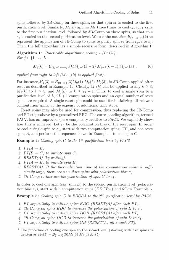
Optimal Algorithmic Cooling of Spins 11
spins followed by 3B-Comp on these spins, so that spin ck is cooled to the firstpurification level. Similarly, M2(k) applies M1 three times to cool ck; ck−1; ck−2
to the first purification level, followed by 3B-Comp on these spins, so that spinck is cooled to the second purification level. We use the notation B(j−1)→j(k) torepresent the application of 3B-Comp to spins to purify spin ck from εj−1 to εj .Then, the full algorithm has a simple recursive form, described in Algorithm 1.
Algorithm 1: Practicable algorithmic cooling 1 (PAC1):For j ∈ {1, . . . , L}
Mj(k) = B{(j−1)−→j}(k)Mj−1(k − 2) Mj−1(k − 1) Mj−1(k) , (6)
applied from right to left (Mj−1(k) is applied first).
For instance,M1(3) = B{0→1}(3)M0(1) M0(2) M0(3), is 3B-Comp applied afterreset as described in Example 1.4 Clearly, M1(k) can be applied to any k ≥ 3,M2(k) to k ≥ 5, and Mj(k) to k ≥ 2j + 1. Thus, to cool a single spin to apurification level of L, 2L+ 1 computation spins and an equal number of resetspins are required. A single reset spin could be used for initializing all relevantcomputation spins, at the expense of additional time steps.
Reset spins may also be used for compression, thus replacing the 3B-Compand PT steps above by a generalized RPC. The corresponding algorithm, termedPAC2, has an improved space complexity relative to PAC1. We explicitly showhow this is achieved. Let ε0 be the polarization bias of the reset spin. In orderto cool a single spin to ε1, start with two computation spins, CB, and one resetspin, A, and perform the sequence shown in Example 4 to cool spin C.
Example 4: Cooling spin C to the 1st purification level by PAC2
1. PT(A→ B).2. PT(B → C) to initiate spin C.3. RESET(A) (by waiting).4. PT(A→ B) to initiate spin B.5. RESET(A). If the thermalization time of the computation spins is suffi-
ciently large, there are now three spins with polarization bias ε0.6. 3B-Comp to increase the polarization of spin C to ε1.
In order to cool one spin (say, spin E) to the second purification level (polariza-tion bias ε2), start with 5 computation spins (EDCBA) and follow Example 5.
Example 5: Cooling spin E in EDCBA to the 2nd purification level by PAC2
1. PT sequentially to initiate spins EDC (RESET(A) after each PT).2. 3B-Comp on spins EDC to increase the polarization of spin E to ε1.3. PT sequentially to initiate spins DCB (RESET(A) after each PT).4. 3B-Comp on spins DCB to increase the polarization of spin D to ε1.5. PT sequentially to initiate spins CB (RESET(A) after each PT).4 The procedure of cooling one spin to the second level (starting with five spins) is
written as M2(5) = B{1→2}(5)M1(3) M1(4) M1(5).

12 Y. Elias et al.
6. 3B-Comp on spins CBA to increase the polarization of spin C to ε1.7. 3B-Comp on spins EDC to increase the polarization of spin E to ε2.
By repeated application of PAC2 in a recursive manner (as for PAC1), spinsystems can be cooled to very low temperatures. PAC1 uses dedicated reset spins,while PAC2 also employs reset spins for compression. The simplest algorithmiccooling can thus be obtained with as few as 3 spins, comprising 2 computationspins and one reset spin.
The algorithms presented so far applied compression steps (3B-Comp) tothree identical biases (ε0); recall that this cools one spin to a new bias, ε′C ≈(3/2)ε0. Now consider applying compression to three spins with different biases(εC , εB, εA); spin C will acquire a new bias ε′C , which is a function of the threeinitial biases [16,17]. This new bias is obtained from the initial probability thatspin C is |0〉 by adding the effect of the exchange |100〉 ↔ |011〉:
1 + ε′C2
=1 + εC
2+ p100 − p011
=1 + εC
2+
1 − εC
21 + εB
21 + εA
2− 1 + εC
21 − εB
21 − εA
2
=1 + εC+εB+εA−εCεBεA
2
2. (7)
The resulting bias is
ε′C =εC + εB + εA − εCεBεA
2, (8)
and in the case where εC , εB, εA � 1,
ε′C ≈ εC + εB + εA
2. (9)
3 Exhaustive Cooling Algorithms
The following examples and derivations are to leading order in the biases. Thisis justified as long as all biases are much smaller than 1, including the finalbiases. For example, with ε0 ∼ 10−5 (ε0 is in the order of magnitude of 10−5)and n ≤ 13, the calculations are fine (see section 4 for details).
3.1 Exhaustive Cooling on Three Spins
Example 6: Fernandez [16]: F(C,B,A,m)Repeat the following m times
1. 3B-Comp(C;B;A), to cool C.2. RESET(B;A)
Consider an application of the primitive algorithm in Example 6 to three spins,C,B,A, where A and B are reset spins with initial biases of εA = εB = ε0 and
Optimal Algorithmic Cooling of Spins 13
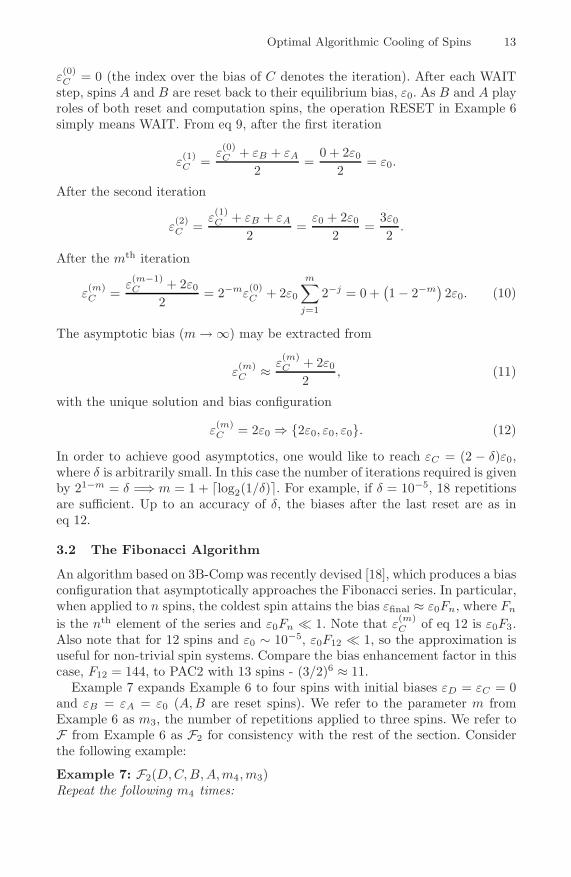
ε(0)C = 0 (the index over the bias of C denotes the iteration). After each WAIT
step, spins A and B are reset back to their equilibrium bias, ε0. As B and A playroles of both reset and computation spins, the operation RESET in Example 6simply means WAIT. From eq 9, after the first iteration
ε(1)C =
ε(0)C + εB + εA
2=
0 + 2ε02
= ε0.
After the second iteration
ε(2)C =
ε(1)C + εB + εA
2=ε0 + 2ε0
2=
3ε02.
After the mth iteration
ε(m)C =
ε(m−1)C + 2ε0
2= 2−mε
(0)C + 2ε0
m∑j=1
2−j = 0 +(1 − 2−m
)2ε0. (10)
The asymptotic bias (m→ ∞) may be extracted from
ε(m)C ≈ ε
(m)C + 2ε0
2, (11)
with the unique solution and bias configuration
ε(m)C = 2ε0 ⇒ {2ε0, ε0, ε0}. (12)
In order to achieve good asymptotics, one would like to reach εC = (2 − δ)ε0,where δ is arbitrarily small. In this case the number of iterations required is givenby 21−m = δ =⇒ m = 1 + �log2(1/δ)�. For example, if δ = 10−5, 18 repetitionsare sufficient. Up to an accuracy of δ, the biases after the last reset are as ineq 12.
3.2 The Fibonacci Algorithm
An algorithm based on 3B-Comp was recently devised [18], which produces a biasconfiguration that asymptotically approaches the Fibonacci series. In particular,when applied to n spins, the coldest spin attains the bias εfinal ≈ ε0Fn, where Fn
is the nth element of the series and ε0Fn � 1. Note that ε(m)C of eq 12 is ε0F3.
Also note that for 12 spins and ε0 ∼ 10−5, ε0F12 � 1, so the approximation isuseful for non-trivial spin systems. Compare the bias enhancement factor in thiscase, F12 = 144, to PAC2 with 13 spins - (3/2)6 ≈ 11.
Example 7 expands Example 6 to four spins with initial biases εD = εC = 0and εB = εA = ε0 (A,B are reset spins). We refer to the parameter m fromExample 6 as m3, the number of repetitions applied to three spins. We refer toF from Example 6 as F2 for consistency with the rest of the section. Considerthe following example:
Example 7: F2(D,C,B,A,m4,m3)Repeat the following m4 times:

14 Y. Elias et al.
1. 3B-Comp(D;C;B), places the new bias on spin D.2. F2(C,B,A,m3).
After each iteration, i, the bias configuration is {ε(i)D , εm3C , ε0, ε0}. Running the
two steps in Example 7 exhaustively (m4,m3 1) yields:
ε(m3)C ≈ 2ε0,
ε(m4)D ≈ εB + ε
(m3)C + ε
(m4)D
2(13)
⇒ ε(m4)D = εB + ε
(m3)C = 3ε0 = ε0F4.
This unique solution was obtained by following the logic of eqs 11 and 12.We generalize this algorithm to n spins An, . . . , A1 in Algorithm 2.
Algorithm 2: Fibonacci F2(An, . . . , A1,mn, ,m3)Repeat the following mn times:
1. 3B-Comp(An;An−1;An−2).2. F2(An−1, . . . , A1,mn−1, . . . ,m3).
[with F2(A3, A2, A1,m3) defined by Example 6.]
Note that different values of mn−1, . . . ,m3 may be applied at each repetitionof step 2 in Algorithm 2. This is a recursive algorithm; it calls itself with oneless spin. Running Algorithm 2 exhaustively (mn,mn−1, . . . ,m3 1) results,similarly to eq 13, in
ε(mn)An
≈ ε(mn)An
+ εAn−1 + εAn−2
2⇒ ε
(mn)An
≈ εAn−1 + εAn−2. (14)
This formula yields the Fibonacci series {. . . , 8, 5, 3, 2, 1, 1}, therefore εAi →ε0Fi. We next devise generalized algorithms which achieve better cooling. Ananalysis of the time requirements of the Fibonacci cooling algorithm is providedin [18].
3.3 The Tribonacci Algorithm
Consider 4-bit-compression (4B-Comp) which consists of an exchange betweenthe states |1000〉 and |0111〉 (the other states remain invariant similar to 3B-Comp). Application of 4B-Comp to four spins D,C,B,A with correspondingbiases εD, εC , εB, εA � 1 results in a spin with the probability of the state |0〉given by
1 + ε′D2
=1 + εD
2+ p|1000〉 − p|0111〉 ≈
1 + εA+εB+εC+3εD
4
2, (15)
following the logic of eqs 7 and 8, and finally
ε′D ≈ (εA + εB + εC + 3εD)/4. (16)

Optimal Algorithmic Cooling of Spins 15
Example 8 applies an algorithm based on 4B-Comp to 4 spins, with initial biasesεD = εC = 0 (A,B are reset spins). In every iteration of Example 8, runningstep 2 exhaustively yields the following biases: εC = 2ε0, εB = εA = ε0. Thecompression step (step 1) is then applied onto the configuration
Example 8: F3(D,C,B,A,m4,m3)Repeat the following m4 times:
1. 4B-Comp(D;C;B;A).2. F2(C,B,A,m3).
From eq 16, ε(i+1)D = (4ε0 + 3ε(i)D )/4. For sufficiently large m4 and m3 the algo-
rithm produces final polarizations of
ε(m4)D ≈ ε0 +
34ε(m4)D =⇒ ε
(m4)D ≈ 4ε0. (17)
For more than 4 spins, a similar 4B-Comp based algorithm may be defined.Example 9 applies an algorithm based on 4B-Comp to 5 spins.
Example 9: F3(E,D,C,B,A,m5,m4,m3)Repeat the following m5 times:
1. 4B-Comp(E;D;C;B).2. F3(D,C,B,A,m4,m3).
Step 2 is run exhaustively in each iteration; the biases of DCBA after this stepare εD = 4ε0, εC = 2ε0, B = A = ε0. The 4B-Comp step is then applied to thebiases of spins (E,D,C,B). Similarly to eq 16, ε(i+1)
E = (7ε0 + 3ε(i)E )/4. Hence,for sufficiently large m5 and m4 the final bias of E is
ε(m5)E ≈ (7ε0 + 3ε(m5)
E )/4 ⇒ ε(m5)E ≈ 7ε0. (18)
Algorithm 3 applies to an arbitrary number of spins n > 4. This is a recursivealgorithm, which calls itself with one less spin.
Algorithm 3: Tribonacci: F3(An, . . . , A1,mn, . . . ,m3)Repeat the following mn times:
1. 4B-Comp(An;An−1;An−2;An−3).2. F3(An−1, . . . , A1,mn−1, . . . ,m3).
[With F3(A4, A3, A2, A1,m4,m3) given by Example 8.]The compression step, 4B-Comp, is applied to
ε(i)An, εAn−1, εAn−2 , εAn−3,
and results in
ε(i+1)An
= (εAn−1 + εAn−2 + εAn−3 + 3ε(i)An)/4. (19)

16 Y. Elias et al.
For sufficiently large mj, j = 3, . . . , n
ε(mn)An
≈ (εAn−1 + εAn−2 + εAn−3 + 3ε(mn)An
)/4
⇒ ε(mn)An
≈ εAn−1 + εAn−2 + εAn−3 . (20)
For εA3 = 2ε0, εA2 = εA1 = ε0, the resulting bias will be ε(mn)An
≈ ε0Tn, whereTn is the nth Tribonacci number.5 As for the Fibonacci algorithm, we assumeε0Tn � 1. The resulting series is {. . . , 24, 13, 7, 4, 2, 1, 1}.
3.4 The k-Bonacci Algorithm
A direct generalization of the Fibonacci and Tribonacci algorithms above isachieved by the application of (k + 1)-bit-compression, or (k + 1)B-Comp. Thiscompression on k+1 spins involves the exchange of |100 · · ·000〉 and |011 · · ·111〉,leaving the other states unchanged. When (k + 1)B-Comp is applied to k + 1spins with biases {εAk+1, εAk
, . . . , εA2 , εA1}, where A1 and A2 are reset spins,the probability that the leftmost spin is |0〉 becomes (similarly to eq 15)
1 + ε′k+1
2=
1 + εk+1
2+p100···000−p011···111 ≈ 1 +
(2k−1−1)εAk+1+∑ k
j=1 εAj
2k−1
2. (21)
Therefore, the bias of the leftmost spin becomes
ε′k+1 ≈ (2k−1 − 1)εAk+1 +∑k
j=1 εAj
2k−1. (22)
Example 10 applies an algorithm based on (k + 1)B-Comp to k + 1 spins. Fk
on k + 1 spins calls (recursively) Fk − 1 on k spins (recall that F3 on four spinscalled F2 on three spins).
Example 10: Fk(Ak+1, . . . , A1,mk+1, . . . ,m3)repeat the following mk+1 times:
1. (k + 1)B-Comp(Ak+1, Ak, . . . , A2, A1)2. Fk−1(Ak, . . . , A1,mk, . . . ,m3)
If step 2 is run exhaustively at each iteration, the resulting biases are
εAk= 2k−2ε0, εAk−1 = 2k−3ε0, . . . , εA3 = 2ε0, εA2 = εA1 = ε0.
The (k+1)B-Comp step is then applied to the biases ε(i)Ak+1, 2k−2ε0, 2k−3ε0, . . . ,
2ε0, ε0, ε0. From eq 22,
ε(i+1)Ak+1
≈(2k−1 − 1)ε(i)Ak+1
+ 2k−1ε0
2k−1.
5 The Tribonacci series (also known as the Fibonacci 3-step series) is generated by therecursive formula ai = ai−1 + ai−2 + ai−3, where a3 = 2 and a2 = a1 = 1.

Optimal Algorithmic Cooling of Spins 17
Hence, for sufficiently large mj, j = 3, . . . , k + 1, the final bias of Ak+1 is
ε(mk+1)Ak+1
≈ (2k−1 − 1)ε(mk+1)Ak+1
+ 2k−1ε0
2k−1⇒ ε
(mk+1)Ak+1
≈ 2k−1ε0. (23)
For more than k + 1 spins a similar (k + 1)B-Comp based algorithm may bedefined. Example 11 applies such an algorithm to k + 2 spins.
Example 11: Fk(Ak+2, . . . , A1,mk+2, . . . ,m3)Repeat the following steps mk+2 times:
1. (k + 1)B-Comp(Ak+2, Ak+1, . . . , A3, A2)2. Fk(Ak+1, . . . , A1,mk+1, . . . ,m3) [defined in Example 11.]
When step 2 is run exhaustively at each iteration, the resulting biases are
εAk+1 = 2k−1ε0, εAk= 2k−2ε0, . . . , εA3 = 2ε0, εA2 = εA1 = ε0.
The (k + 1)B-Comp is applied to the biases. From Eq. 22,
ε(i+1)Ak+2
=(2k−1 − 1)ε(i)Ak+2
+ (2k − 1)ε02k−1
.
Hence, for sufficiently large mj , j = 3, . . . , k + 2, the final bias of Ak+2 is
ε(mk+2)Ak+2
≈(2k−1 − 1)ε(mk+2)
Ak+2+ (2k − 1)ε0
2k−1⇒ ε
(mk+2)Ak+2
≈ (2k − 1)ε0. (24)
Algorithm 4 generalizes Examples 10 and 11.
Algorithm 4: k-bonacci: Fk(An, . . . , A1,mn, . . . ,m3)Repeat the following mn times:
1. (k + 1)B-Comp(An, An−1, . . . , An−k).2. Fk(An−1, . . . , A1,mn−1, . . . ,m3).
[with Fk(Ak+1, . . . , A1,mk+1, . . . ,m3) defined in Example 10.]
The algorithm is recursive; it calls itself with one less spin. The compressionstep, (k + 1)B-Comp, is applied to
ε(i)An, εAn−1 , . . . εAn−k
.
From Eq. 22, the compression results in
ε(i+1)An
≈ (2k−1 − 1)ε(i)An+
∑kj=1 εAn−j
2k−1. (25)
For sufficiently large mn,mn−1, etc.
ε(mn)An
≈ (2k−1 − 1)ε(mn)An
+∑k
j=1 εAn−j
2k−1
⇒ ε(mn)An
≈k∑
j=1
εAn−j (26)

18 Y. Elias et al.
This set of biases corresponds to the k-step Fibonacci sequence which is gener-ated by a recursive formula.
a1, a2 = 1, a� =
⎧⎨⎩
∑�−1i=1 a�−i, 3 ≤ � ≤ k + 1
∑ki=1 a�−i � > k + 1
⎫⎬⎭ . (27)
Notice that for 3 ≤ � ≤ k + 1,
a� =�−1∑i=1
ai = 1 + 1 + 2 + 4 + · · · + 2�−4 + 2�−3 = 2�−2. (28)
The algorithm uses �-bit-compression (�-B-Comp) gates, where 3 ≤ � ≤ k + 1.
3.5 The All-Bonacci Algorithm
In Example 11 (Fk applied to k + 1 spins), the resulting biases of the com-putation spins, 2k−1ε0, 2k−2ε0, . . . , 2ε0, ε0, were proportional to the exponentialseries {2k−1, 2k−2, . . . , 4, 2, 1}. For example, F2 on 3 spins results in {2ε0, ε0, ε0}(see Example 6), and F3 on 4 spins results in {4ε0, 2ε0, ε0, ε0} (see Example 8).This coincides with the k-step Fibonacci sequence, where a� = 2�−2, for a1 = 1and � = 2, 3, ..., k+1 (see eq 28). This property leads to cooling of n+1 spins bya special case of k-bonacci (Algorithm 5), where k-bonacci is applied to k = n−1spins.
Algorithm 5: All-bonacci: FAll(An, . . . , A1,mn . . . ,m3)Apply Fn−1(An, . . . , A1,mn, . . . ,m3).
The final biases after all-bonacci are εAi → ε02i−2 for i > 1. The resulting seriesis {. . . , 16, 8, 4, 2, 1, 1}.
The all-bonacci algorithm potentially constitutes an optimal AC scheme, asexplained in section 4.
3.6 Density Matrices of the Cooled Spin Systems
For a spin system in a completely mixed state, the density matrix of eachspin is:
12I =
12
(1
1
). (29)
The density matrix of the entire system, which is diagonal, is given by the tensorproduct ρCM = 1
23 I ⊗ I ⊗ I, where
Diag(ρCM) = 2−3(1, 1, 1, 1, 1, 1, 1, 1). (30)
For three spins in a thermal state, the density matrix of each spin is
ρ(1)T =
12
(1 + ε0
1 − ε0
). (31)

Optimal Algorithmic Cooling of Spins 19
and the density matrix of the entire system is given by the tensor product ρT =ρ(1)T ⊗ ρ
(1)T ⊗ ρ
(1)T . This matrix is also diagonal. We write the diagonal elements
to leading order in ε0:
Diag(ρT ) = 2−3(1+3ε0, 1+ε0, 1+ε0, 1+ε0, 1−ε0, 1−ε0, 1−ε0, 1−3ε0). (32)
Consider now the density matrix after shifting and scaling, ρ′ = 2n(ρ−2−nI)/ε0.For any Diag(ρ) = (p1, p2, p3, . . . , pn) the resulting diagonal is Diag(ρ′) =(p′1, p
′2, p′3, . . . , p
′n) with p′j = 2n(pj − 2−n)/ε0. The diagonal of a shifted and
scaled (S&S) matrix for a completely mixed state (eq 30) is
Diag(ρ′CM ) = (0, 0, 0, 0, 0, 0, 0, 0), (33)
and for a thermal state (eq. 32)
Diag(ρ′T ) = (3, 1, 1, 1,−1,−1,−1,−3). (34)
In the following discussion we assume that any element, p, satisfies p′ε0 � 1.When applied to a diagonal matrix with elements of the form p = 1
2n (1 ± p′iε0),this transformation yields the corresponding S&S elements, ± p′i.
Consider now the application of the Fibonacci to three spins. The resultantbias configuration, {2ε0, ε0, ε0} (eq 12) is associated with the density matrix
ρ(3)Fib =
123
(1 + 2ε0
1 − 2ε0
)⊗
(1 + ε0
1 − ε0
)⊗
(1 + ε0
1 − ε0
), (35)
with a corresponding diagonal, to leading order in ε0,
Diag(ρ(3)Fib
)= 2−3 (1 + 4ε0, 1 + 2ε0, 1 + 2ε0, 1, 1, 1 − 2ε0, 1 − 2ε0, 1 − 4ε0) .
(36)The S&S form of this diagonal is
Diag(ρ′(3)Fib
)= (4, 2, 2, 0, 0,−2,−2,−4) . (37)
Similarly, the S&S diagonal for Tribonacci on four spins is
Diag(ρ′(4)Trib
)= (8, 6, 6, 4, 4, 2, 2, 0, 0,−2,−2,−4,−4,−6,−6,−8) . (38)
and the S&S form of the diagonal for all-bonacci on n spins is
Diag(ρ′(n)
allb
)=
[2n−1, (2n−1 − 2), (2n−1 − 2), . . . , 2, 2, 0, 0, . . . ,−2n − 1
]. (39)
which are good approximations as long as 2nε0 � 1.
Partner Pairing Algorithm. Recently a cooling algorithm was devised thatachieves a superior bias than previous AC algorithms. [18,19] This algorithm,termed the Partner Pairing Algorithm (PPA), was shown to produce the highest

20 Y. Elias et al.
possible bias for an arbitrary number of spins after any number of reset steps.Let us assume that the reset spin is the least significant bit (the rightmost spin inthe tensor-product density matrix). The PPA on n spins is given in Algorithm 6.
Algorithm 6: Partner Pairing Algorithm (PPA)Repeat the following, until cooling arbitrarily close to the limit.
1. RESET – applied only to a single reset spin.2. SORT – A permutation that sorts the 2n diagonal elements of the density
matrix by decreasing value, such that p0 is the largest, and p2n−1 is thesmallest.
Written in terms of ε, the reset step has the effect of changing the traced densitymatrix of the reset spin to
ρε =1
eε + e−ε
(eε
e−ε
)=
12
(1 + ε0
1 − ε0
), (40)
for any previous state. From eq 40 it is clear that ε0 = tanh ε as stated in theintroduction. For a single spin in any diagonal mixed state:
(p0
p1
)RESET−−−−−→ p0 + p1
2
(1 + ε0
1 − ε0
)=
12
(1 + ε0
1 − ε0
). (41)
For two spins in any diagonal state a reset of the least significant bit results in⎛⎜⎜⎝p0
p1
p2
p3
⎞⎟⎟⎠
RESET−−−−−→
p0 + p1
2
⎛⎜⎜⎝
p0+p12 (1 + ε0)
p0+p12 (1 − ε0)
p2+p32 (1 + ε0)
p2+p32 (1 − ε0)
⎞⎟⎟⎠ . (42)
Algorithm 6 may be highly inefficient in terms of logic gates. Each SORT couldrequire an exponential number of gates. Furthermore, even calculation of therequired gates might be exponentially hard.
We refer only to diagonal matrices and the diagonal elements of the matrices(applications of the gates considered here to a diagonal density matrix do notproduce off-diagonal elements). For a many-spin system, RESET of the resetspin, transforms the diagonal of any diagonal density matrix, ρ, as follows:
Diag(ρ) = (p0, p1, p2, p3, . . .) → (43)[p0 + p1
2(1 + ε0),
p0 + p1
2(1 − ε0),
p2 + p3
2(1 + ε0),
p2 + p3
2(1 − ε0), . . .
],
as the density matrix of each pair, pi and pi+1 (for even i) is transformed bythe RESET step as described by eq 40 above. We use the definition of S&Sprobabilities, p′ = 2n(p− 2−n)/ε0. The resulting S&S diagonal is

Optimal Algorithmic Cooling of Spins 21
Diag(ρ′) =[2n
ε0
(p0 + p1
2+ (1 + ε0) − 2−n
), . . .
]=
[2n
ε0
(p0 + p1
2− 2−n
)+ 2n p0 + p1
2, . . .
]=
[p′1 + p′2
2+ 1,
p′0 + p′12
+ 2n p0 + p1
2,p′0 + p′1
2− 2n p0 + p1
2, . . .
], (44)
where the second element is shown in the final expression. We now use p =2−n(ε0p′ + 1), to obtain
2n p0 + p1
2= 2n 2−n(ε0p′0 + 1) + 2−n(ε0p′1 + 1)
2(45)
=ε0(p′0 + p′1) + 2
2= 1 + ε0
p′0 + p′12
. (46)
Ref [18] provides an analysis of the PPA. We continue, as in the previous sub-section, to analyze the case of p′ε0 � 1, which is of practical interest. In thiscase 1+ ε0
p′0+p′
12 ≈ 1. Hence, the effect of a RESET step on the S&S diagonal is:
Diag(ρ′) = (p′0, p′1, p′2, p′3, . . .) → (47)[
p′0 + p′12
+ 1,p′0 + p′1
2− 1,
p′2 + p′32
+ 1,p′2 + p′3
2− 1, . . .
]
Consider now three spins, such that the one at the right is a reset spin. Followingref [18], we initially apply the PPA to three spins which are initially at thecompletely mixed state. The first step of the PPA, RESET (eq 47), is appliedto the diagonal of the completely mixed state (eq 33), to yield
Diag(ρ′CMS) → Diag(ρ′RESET ) = (1,−1, 1,−1, 1,−1, 1,−1). (48)
This diagonal corresponds to the density matrix
ρRESET =123
I ⊗ I ⊗(
1 + ε01 − ε0
), (49)
namely to the bias configuration {0, 0, ε0}. The next PPA step, SORT, sorts thediagonal elements in decreasing order:
Diag(ρ′SORT ) = (1, 1, 1, 1,−1,−1,−1,−1), (50)
that arises from the density matrix
ρSORT =123
(1 + ε0
1 − ε0
)⊗ I ⊗ I, (51)
which corresponds to the biases {ε0, 0, 0}. The bias was thus transferred to theleftmost spin. In the course of repeated alternation between the two steps of thePPA, this diagonal will further evolve as detailed in Example 12.

22 Y. Elias et al.
The rightmost column of Example 12 lists the resulting bias configurations.Notice that after the 5th step the biases are identical. Also notice that in the 6th
and 10th steps the states |100〉 and |011〉 are exchanged (3B-Comp); after boththese steps, the state of the system cannot be written as a tensor product.6 Alsonotice that after step 13, the PPA applies a SORT which will also switch betweenthese two states. The PPA, applied to the bias configuration {tε0, ε0, ε0}, where1 ≤ t ≤ 2 is simply an exchange |100〉 ↔ |011〉 . This is evident from the diagonal
Diag(ρ′) = (t+ 2, t, t, t− 2,−t+ 2,−t,−t,−t− 2). (52)
Thus, the PPA on three spins is identical to the Fibonacci algorithm applied tothree spins (see Example 6). This analogy may be taken further to some extent.When the PPA is applied onto four spins, the outcome, but not the steps, isidentical to the result obtained by Tribonacci algorithm (see Example 8). Theseidentical results may be generalized to the PPA and all-bonacci applied onton ≥ 3 spins.
Example 12: Application of PPA to 3 spins
Diag(ρ′) = (0, 0, 0, 0, 0, 0, 0, 0) {0, 0, 0}step 1 RESET−−−−−→ (1,−1, 1,−1, 1,−1, 1,−1) {0, 0, ε0}step 2 SORT−−−−→ (1, 1, 1, 1,−1,−1,−1,−1) {ε0, 0, 0}step 3 RESET−−−−−→ (2, 0, 2, 0, 0,−2, 0,−2) {ε0, 0, ε0}step 4 SORT−−−−→ (2, 2, 0, 0, 0, 0,−2,−2) {ε0, ε0, 0}step 5 RESET−−−−−→ (3, 1, 1,−1, 1,−1,−1,−3) {ε0, ε0, ε0}step 6 SORT−−−−→ (3, 1, 1, 1,−1,−1,−1,−3) N. A.
step 7 RESET−−−−−→ (3, 1, 2, 0, 0,−2,−1,−3) { 3ε02 , ε0
2 , ε0}step 8 SORT−−−−→ (3, 2, 1, 0, 0,−1,−2,−3) { 3ε0
2 , ε0,ε02 }
step 9 RESET−−−−−→ 12 (7, 3, 3,−1, 1,−3,−3,−7) { 3ε0
2 , ε0, ε0}step 10 SORT−−−−→ 1
2 (7, 3, 3, 1,−1,−3,−3,−7) N.A.
step 11 RESET−−−−−→ 12 (7, 3, 4, 0, 0,−4,−3,−7) { 7ε0
4 , 3ε04 , ε0}
step 12 SORT−−−−→ 12 (7, 4, 3, 0, 0,−3,−4,−7) { 7ε0
4 , ε0,3ε04 }
step 13 RESET−−−−−→ 14 (15, 7, 7,−1, 1,−7,−7,−15) { 7ε0
4 , ε0, ε0}
4 Optimal Algorithmic Cooling
4.1 Lower Limits of the PPA and All-Bonacci
Consider an application of the PPA to a three-spin system at a state with theS&S diagonal of eq 37. This diagonal is both sorted and invariant to RESET,
6 This is due to classical correlations (not involving entanglement) between the spins;an individual bias may still be associated with each spin by tracing out the others,but such a bias cannot be interpreted as temperature.

Optimal Algorithmic Cooling of Spins 23
hence it is invariant to the PPA. Eq 37 corresponds to the bias configura-tion {2ε0, ε0, ε0} which is the limit of the Fibonacci algorithm presented above(eq 12). This configuration is the “lower” limit of the PPA with three spins inthe following sense: any “hotter configuration” is not invariant and continues tocool down during exhaustive PPA until reaching or bypassing this configuration.For four spins the diagonal of Eq 38 is invariant to the PPA for the same reasons.This diagonal corresponds to the bias configuration {4ε0, 2ε0, ε0, ε0}, which isthe limit of the Tribonacci algorithm (or the all-bonacci) applied to four spins.Any “hotter configuration” is not invariant and cools further during exhaustivePPA, until it reaches (or bypasses) this configuration.
Now, we follow the approximation of very small biases for n spins, where2nε0 � 1. The diagonal in eq 39 is invariant to the PPA. This diagonal corre-sponds to the bias configuration
{2n−2ε0, 2n−3ε0, 2n−4ε0, . . . , 2ε0, ε0, ε0}, (53)
which is the limit of the all-bonacci algorithm. As before, any “hotter configura-tion” is not invariant and cools further. It is thus proven that the PPA reachesat least the same biases as all-bonacci.
We conclude that under the assumption 2nε0 � 1, the n-spin system can becooled to the bias configuration shown in eq 53. When this assumption is notvalid (e.g., for larger n with the same ε0), pure qubits can be extracted; seetheorem 2 in [19] (theorem 3 in ref [18]).
Yet, the PPA potentially yields “colder configurations”. We obtained numer-ical results for small spin systems which indicate that the limits of the PPA andall-bonacci are identical. Still, since the PPA may provide better cooling, it isimportant to put an “upper” limit on its cooling capacity.
4.2 Upper Limits on Algorithmic Cooling
Theoretical limits for cooling with algorithmic cooling devices have recently beenestablished [18,19]. For any number of reset steps, the PPA has been shown to beoptimal in terms of entropy extraction (see ref [19] and more details in section 1of ref [18]). An upper bound on the degree of cooling attainable by the PPAis therefore also an upper bound of any AC algorithm. The following theoremregards a bound on AC which is the loose bound of ref [18].
Theorem 1. No algorithmic cooling method can increase the probability of anybasis state to above7 min{2−ne2
nε, 1}, where the initial configuration is the com-pletely mixed state.8 This includes the idealization where an unbounded numberof reset and logic steps can be applied without error or decoherence.
The proof of Theorem 1 involves applying the PPA and showing that the prob-ability of any state never exceeds 2−ne2
nε.
7 A tighter bound, p0 ≤ 2−ne2n−1ε, was claimed by theorem 1 of ref [18].8 It is assumed that the computation spins are initialized by the polarization of the
reset spins.
24 Y. Elias et al.
5 Algorithmic Cooling and NMR Quantum Computing
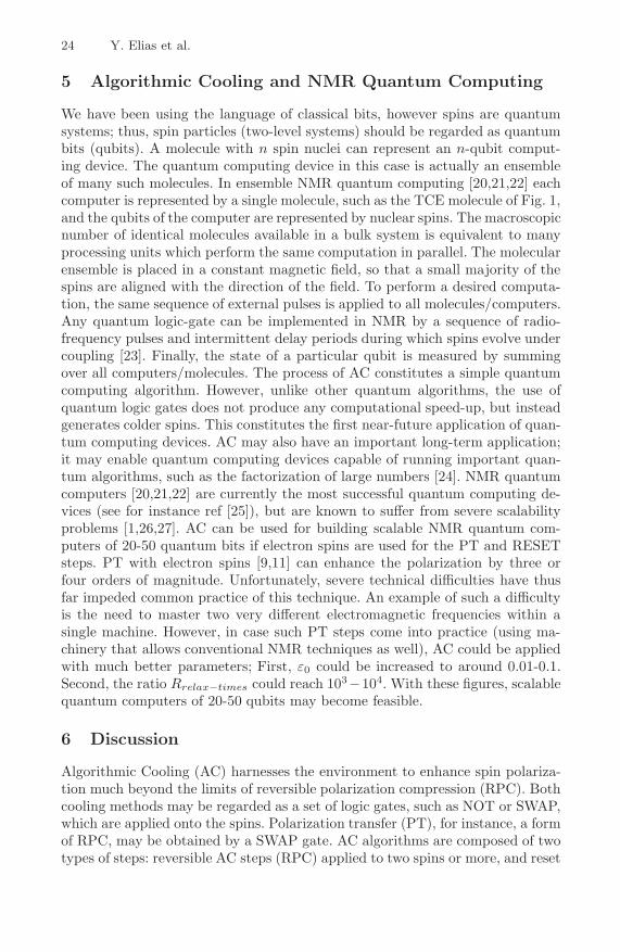
We have been using the language of classical bits, however spins are quantumsystems; thus, spin particles (two-level systems) should be regarded as quantumbits (qubits). A molecule with n spin nuclei can represent an n-qubit comput-ing device. The quantum computing device in this case is actually an ensembleof many such molecules. In ensemble NMR quantum computing [20,21,22] eachcomputer is represented by a single molecule, such as the TCE molecule of Fig. 1,and the qubits of the computer are represented by nuclear spins. The macroscopicnumber of identical molecules available in a bulk system is equivalent to manyprocessing units which perform the same computation in parallel. The molecularensemble is placed in a constant magnetic field, so that a small majority of thespins are aligned with the direction of the field. To perform a desired computa-tion, the same sequence of external pulses is applied to all molecules/computers.Any quantum logic-gate can be implemented in NMR by a sequence of radio-frequency pulses and intermittent delay periods during which spins evolve undercoupling [23]. Finally, the state of a particular qubit is measured by summingover all computers/molecules. The process of AC constitutes a simple quantumcomputing algorithm. However, unlike other quantum algorithms, the use ofquantum logic gates does not produce any computational speed-up, but insteadgenerates colder spins. This constitutes the first near-future application of quan-tum computing devices. AC may also have an important long-term application;it may enable quantum computing devices capable of running important quan-tum algorithms, such as the factorization of large numbers [24]. NMR quantumcomputers [20,21,22] are currently the most successful quantum computing de-vices (see for instance ref [25]), but are known to suffer from severe scalabilityproblems [1,26,27]. AC can be used for building scalable NMR quantum com-puters of 20-50 quantum bits if electron spins are used for the PT and RESETsteps. PT with electron spins [9,11] can enhance the polarization by three orfour orders of magnitude. Unfortunately, severe technical difficulties have thusfar impeded common practice of this technique. An example of such a difficultyis the need to master two very different electromagnetic frequencies within asingle machine. However, in case such PT steps come into practice (using ma-chinery that allows conventional NMR techniques as well), AC could be appliedwith much better parameters; First, ε0 could be increased to around 0.01-0.1.Second, the ratio Rrelax−times could reach 103−104. With these figures, scalablequantum computers of 20-50 qubits may become feasible.
6 Discussion
Algorithmic Cooling (AC) harnesses the environment to enhance spin polariza-tion much beyond the limits of reversible polarization compression (RPC). Bothcooling methods may be regarded as a set of logic gates, such as NOT or SWAP,which are applied onto the spins. Polarization transfer (PT), for instance, a formof RPC, may be obtained by a SWAP gate. AC algorithms are composed of twotypes of steps: reversible AC steps (RPC) applied to two spins or more, and reset

Optimal Algorithmic Cooling of Spins 25
steps, in which entropy is shifted to the environment through reset spins. Thesereset spins thermalize much faster than computation spins (which are cooled),allowing a form of a molecular heat pump. A prerequisite for AC is thus themutual existence (on the same molecule) of two types of spins with a substantialrelaxation times ratio (of at least an order of magnitude). While this demandlimits the applicability of AC, it is often met in practice (e.g., by 1H vs 13C incertain organic molecules) and may be induced by the addition of a paramag-netic reagent. The attractive possibility of using rapidly-thermalizing electronspins as reset bits is gradually becoming a relevant option for the far future.
We have surveyed previous cooling algorithms and suggested novel algorithmsfor exhaustive AC: the Tribonacci, the k-bonacci, and the all-bonacci algorithms.We conjectured the optimality of all-bonacci, as it appears to yield the samecooling level as the PPA of refs [18,19]. Improving the SNR of NMR by ACpotentially constitutes the first short-term application of quantum computingdevices. AC is further accommodated in quantum computing schemes (NMR-based or others) relating to the more distant future [1,28,29,30].
Acknowledgements
Y.E., T.M., and Y.W. thank the Israeli Ministry of Defense, the Promotion ofResearch at the Technion, and the Institute for Future Defense Research forsupporting this research.
References
1. Boykin, P.O., Mor, T., Roychowdhury, V., Vatan, F., Vrijen, R.: Algorithmic cool-ing and scalable NMR quantum computers. Proc. Natl. Acad. Sci. 99(6), 3388–3393(2002)
2. Fernandez, J.M., Lloyd, S., Mor, T., Rowchoudury, V.: Algorithmic cooling of spins:A practicable method for increasing polarisation. Int. J. Quant. Inf. 2(4), 461–467(2004)
3. Mor, T., Roychowdhury, V., Lloyd, S., Fernandez, J.M., Weinstein, Y.: US patentNo. 6,873,154 (2005)
4. Cover, T.M., Thomas, J.A.: Elements of Information Theory. Wiley, New York(1991)
5. Brassard, G., Elias, Y., Fernandez, J.M., Gilboa, H., Jones, J.A., Mor, T., Wein-stein, Y., Xiao, L.: Experimental heat-bath cooling of spins. Proc. Natl. Acad. Sci.USA (submitted) (also in arXiv:quant-ph/0511156)
6. Morris, G.A., Freeman, R.: Enhancement of nuclear magnetic resonance signals bypolarization transfer. J. Am. Chem. Soc. 101, 760–762 (1979)
7. Sørensen, O.W.: Polarization transfer experiments in high-resolution NMR spec-troscopy. Prog. Nucl. Mag. Res. Spec. 21, 503–569 (1989)
8. Schulman, L.J., Vazirani, U.V.: Scalable NMR quantum computation. In: ACMSymposium on the Theory of Computing (STOC): Proceedings, pp. 322–329. ACMPress, New York (1999)
9. Farrar, C.T., Hall, D.A., Gerfen, G.J., Inati, S.J., Griffin, R.G.: Mechanism ofdynamic nuclear polarization in high magnetic fields. J. Chem. Phys. 114, 4922–4933 (2001)

26 Y. Elias et al.
10. Slichter, C.P.: Principles of Magnetic Resonance, 3rd edn. Springer, Heidelberg(1990)
11. Ardenkjær-Larsen, J.H., Fridlund, B., Gram, A., Hansson, G., Hansson, L., Lerche,M.H., Servin, R., Thaning, M., Golman, K.: Increase in signal-to-noise ratio of> 10, 000 times in liquid-state NMR. Proc. Natl. Acad. Sci. 100, 10158–10163(2003)
12. Anwar, M., Blazina, D., Carteret, H., Duckett, S.B., Halstead, T., Jones, J.A.,Kozak, C., Taylor, R.: Preparing high purity initial states for nuclear magneticresonance quantum computing. Phys. Rev. Lett. 93 (2004) (also in arXiv:quant-ph/0312014)
13. Oros, A.M., Shah, N.J.: Hyperpolarized xenon in NMR and MRI. Phys. Med.Biol. 49, R105–R153 (2004)
14. Emsley, L., Pines, A.: Lectures on pulsed NMR. In: Nuclear Magnetic DoubleResonance, Proceedings of the CXXIII School of Physics Enrico Fermi, 2nd edn.p. 216. World Scientific, Amsterdam (1993)
15. Elias, Y., Fernandez, J.M., Mor, T., Weinstein, Y.: Algorithmic cooling of spins.Isr. J. Chem. (to be published on 2007)
16. Fernandez, J.M.: De computatione quantica. PhD thesis, University of Montreal,Canada (2003)
17. Weinstein, Y.: Quantum computation and algorithmic cooling by nuclear mag-netic resonance. Master’s thesis, Physics Department, Technion - Israel Instituteof Technology (August 2003)
18. Schulman, L.J., Mor, T., Weinstein, Y.: Physical limits of heat-bath algorithmiccooling. SIAM J. Comp. 36, 1729–1747 (2007)
19. Schulman, L.J., Mor, T., Weinstein, Y.: Physical limits of heat-bath algorithmiccooling. Phys. Rev. Lett. 94, 120501 (2005)
20. Cory, D.G., Fahmy, A.F., Havel, T.F.: Nuclear magnetic resonance spectroscopy:an experimentally accessible paradigm for quantum computing. In: Proceedings ofPhysComp96, pp. 87–91 (1996)
21. Cory, D.G., Fahmy, A.F., Havel, T.F.: Ensemble quantum computing by nuclearmagnetic resonance spectroscopy. Proc. Natl. Acad. Sci. 1634–1639 (1997)
22. Gershenfeld, N.A., Chuang, I.L.: Bulk spin-resonance quantum computation. Sci-ence 275, 350–356 (1997)
23. Price, M.D., Havel, T.F., Cory, D.G.: Multiqubit logic gates in NMR quantumcomputing. New Journal of Physics 2, 10.1–10.9 (2000)
24. Shor, P.W.: Polynomial-time algorithms for prime factorization and discrete loga-rithms on a quantum computer. SIAM J. Comp. 26(5), 1484–1509 (1997)
25. Vandersypen, L.M.K., Steffen, M., Breyta, G., Yannoni, C.S., Sherwood, M.H.,Chuang, I.L.: Experimental realization of Shor’s quantum factoring algorithm usingnuclear magnetic resonance. Nature 414, 883–887 (2001)
26. Warren, W.S.: The usefulness of NMR quantum computing. Science 277, 1688–1690(1997)
27. DiVincenzo, D.P.: Real and realistic quantum computers. Nature 393, 113–114(1998)
28. Twamley, J.: Quantum-cellular-automaton quantum computing with endohedalfullerenes. Phys. Rev. A 67, 052318 (2003)
29. Freegarde, T., Segal, D.: Algorithmic cooling in a momentum state quantum com-puter. Phys. Rev. Lett. 91, 037904 (2003)
30. Ladd, T.D., Goldman, J.R., Yamaguchi, F., Yamamoto, Y., Abe, E., Itoh, K.M.:All-silicon quantum computer. Phys. Rev. Lett. 89, 017901 (2002)

Nanocomputing by Self-assembly
Lila Kari
Department of Computer ScienceUniversity of Western Ontario
London, OntarioCanada N6A [email protected]
Abstract. Biomolecular (DNA) computing is an emergent field of un-conventional computing, lying at the crossroads of mathematics, com-puter science and molecular biology. The main idea behind biomolecularcomputing is that data can be encoded in DNA strands, and techniquesfrom molecular biology can be used to perform arithmetic and logic op-erations. The birth of this field was the 1994 breakthrough experimentof Len Adleman who solved a hard computational problem solely bymanipulating DNA strands in test-tubes. This led to the possibility ofenvisaging a DNA computer that could be thousand to a million timesfaster, trillions times smaller and thousand times more energy efficientthan today’s electronic computers.
I will present one of the most active directions of research in DNAcomputing, namely DNA nanocomputing by self-assembly. I will namelydiscuss the computational potential of self-assembly, the process by whichobjects autonomously come together to form complex structures. I willbring forth evidence that self-assembly of DNA molecules can be used toperform computational tasks. Lastly, I will address the problem of self-assembly of arbitrarily large super-shapes, its solution and implications.
S.G. Akl et al.(Eds.): UC 2007, LNCS 4618, p. 27, 2007.c© Springer-Verlag Berlin Heidelberg 2007

Organic User Interfaces (Oui!):
Designing Computers inAny Way Shape or Form
Roel Vertegaal
Xuuk Inc. / Human Media LaboratorySchool of Computing, Queen’s University
Kingston, OntarioCanada K7L [email protected]
Abstract. Over the past few years, there has been a quiet revolutionin display manufacturing technology. One that is only comparable inscope to that of the invention of the first LCD, which led to DynaBookand the modern laptop. E-ink electrophoretic pixel technology, combinedwith advances in organic thin-film circuit substrates, have led to displaysthat are so thin and flexible they are beginning to resemble paper. Soondisplays will completely mimic the high contrast, low power consumptionand flexibility of printed media. As with the invention of the first LCD,this means we are on the brink of a new paradigm in computer userinterface design: one in which computers can have any organic form orshape. One where any object, no matter how complex, dynamic or flexibleits structure, may display information. One where the deformation ofshape is a main source of input.
This new paradigm of Organic User Interface (Oui!) requires a newset of design guidelines, which I will discuss in this presentation. Theseguidelines were inspired by architecture, which went through a similartransformation decades ago. In Oui! The Input Device Is The OutputDevice (TIDISTOD), Form dynamically follows Flow of activities of thehuman body, and Function equals Form. I will give an overview of tech-nologies that led to Organic UI, such as Tangible UI and Digital Desks,after which I will discuss some of the first real Oui! interfaces, which in-clude Gummi and PaperWindows. PaperWindows, which was developedat HML, is the first real paper computer. It uses computer vision to tracksheets of real paper in real time. Page shape is modeled in 3D, texturedwith windows and projected back onto the paper, making for a wirelesshi-res flexible color display. Interactions with PaperWindows take placethrough hand gestures and paper folding techniques.
S.G. Akl et al.(Eds.): UC 2007, LNCS 4618, p. 28, 2007.c© Springer-Verlag Berlin Heidelberg 2007
Unconventional Models of Computation
Through Non-standard Logic Circuits
Juan C. Agudelo1 and Walter Carnielli2
1 Ph.D. Program in Philosophy/LogicIFCH and Group for Applied and Theoretical Logic- CLE
State University of Campinas - UNICAMP, Brazil2 IFCH and Group for Applied and Theoretical Logic- CLE
State University of Campinas - UNICAMP, BrazilSQIG - IT, Portugal
{juancarlos,carniell}@cle.unicamp.br
Abstract. The classical (boolean) circuit model of computation isgeneralized via polynomial ring calculus, an algebraic proof methodadequate to non-standard logics (namely, to all truth-functional propo-sitional logics and to some non-truth-functional logics). Such generaliza-tion allows us to define models of computation based on non-standardlogics in a natural way by using ‘hidden variables’ in the constitution ofthe model. Paraconsistent circuits for the paraconsistent logic mbC (andfor some extensions) are defined as an example of such models. Some po-tentialities are explored with respect to computability and computationalcomplexity.
1 Introduction
The classical notion of algorithm is founded in the model of automated ma-chines introduced by Turing in [18], now known as Turing machines, and in itsequivalent theories (λ-definability, partial recursive functions, uniform familiesof boolean circuits, and so on). Surprising connections between classical logicand classical computation have been established, as the equivalence between thewell-known ‘halting problem’ and the undecidability of first-order logic (see [18],[3] and [2]), and the relationship between computational complexity and express-ibility in logic (see [15, sec. 2] for a survey). The advent of so many non-classicallogics challenge us to think, prompted by the above connections, in the possibil-ities of logic relativization of the notion of computability and in its conceivableadvantages. In this spirit we presented in [1] a model of ‘paraconsistent Turingmachines’, a generalization of Turing machines through a paraconsistent logic,and proved that some characteristics of quantum computation can be simulatedby this kind of machines. In particular, we have showed how this model can beused to solve the so-called Deutsch-Jozsa problem in an efficient way. In thispaper we propose another generalization of a classical model of computation(boolean circuits), defining unconventional models of logic circuits where gateoperations are defined in accordance with adequate semantics for non-classical
S.G. Akl et al.(Eds.): UC 2007, LNCS 4618, pp. 29–40, 2007.c© Springer-Verlag Berlin Heidelberg 2007
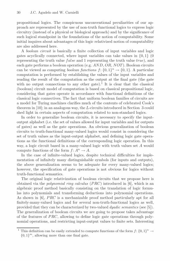
30 J.C. Agudelo and W. Carnielli
propositional logics. The conspicuous unconventional peculiarities of our ap-proach are represented by the use of non-truth functional logics to express logiccircuitry (instead of a physical or biological approach) and by the significance ofsuch logical standpoint in the foundations of the notion of computability. Someinitial inquires about advantages of this logic relativized notion of computabilityare also addressed here.
A boolean circuit is basically a finite collection of input variables and logicgates acyclically connected, where input variables can take values in {0, 1} (0representing the truth value false and 1 representing the truth value true), andeach gate performs a boolean operation (e.g. AND, OR, NOT ). Boolean circuitscan be viewed as computing boolean functions f : {0, 1}n → {0, 1}. A particularcomputation is performed by establishing the values of the input variables andreading the result of the computation as the output at the final gate (the gatewith no output connections to any other gate).1 It is clear that the classical(boolean) circuit model of computation is based on classical propositional logic,considering that gates operate in accordance with functional definitions of theclassical logic connectives. The fact that uniform boolean families of circuits area model for Turing machines clarifies much of the contents of celebrated Cook’stheorem in [10]; in an analogous way, the L-circuits introduced in Section 3 couldshed light in certain aspects of computation related to non-standard logics.
In order to generalize boolean circuits, it is necessary to specify the input-output alphabet (i.e. the set of values allowed for input variables and for outputsof gates) as well as the gate operations. An obvious generalization of booleancircuits to truth-functional many-valued logics would consist in considering theset of truth values as the input-output alphabet, and defining logic gate opera-tions as the functional definitions of the corresponding logic operation. In thisway, a logic circuit based in a many-valued logic with truth values set A wouldcompute functions of the form f : An → A.
In the case of infinite-valued logics, despite technical difficulties for imple-mentation of infinitely many distinguishable symbols (for inputs and outputs),the above generalization seems to be adequate for every many-valued logics;however, the specification of gate operations is not obvious for logics withouttruth-functional semantics.
The original logic relativization of boolean circuits that we propose here isobtained via the polynomial ring calculus (PRC) introduced in [6], which is analgebraic proof method basically consisting on the translation of logic formu-las into polynomials and transforming deductions into polynomial operations.As shown in [6], PRC is a mechanizable proof method particularly apt for allfinitely-many-valued logics and for several non-truth-functional logics as well,provided that they can be characterized by two-valued dyadic semantics (see [5]).The generalization of boolean circuits we are going to propose takes advantageof the features of PRC, allowing to define logic gate operations through poly-nomial operations, and restricting input-output values to finite sets. Interesting
1 This definition can be easily extended to compute functions of the form f : {0, 1}n →{0, 1}m, allowing more than one final gate.

Unconventional Models of Computation 31
examples of our generalization are presented by exhibiting PRC for the paracon-sistent logic mbC and for some extensions, while exploring some potentialitiesof this model with respect to computability and computational complexity.
We present a summary of the PRC proof method and some illustrative ex-amples following [6], before presenting the promised generalization of booleancircuits.
2 Polynomial Ring Calculus
PRC consists in translating logic formulas into polynomials over the finite (Ga-lois) fields GF (pn) (where p is a prime number and n is a natural number).2
PRC defines rules to operate with polynomials. The first group of rules, thering rules, correspond to the ring properties of addition and multiplication: ad-dition is associative and commutative, there is a ‘zero’ element and all elementshave ‘addition inverse’; multiplication is associative, and there is a ‘one’ ele-ment and multiplication distributes over addition. The second group of rules,the polynomial rules, establishes that the addition of an element x exactlypn times can be reduced to the constant polynomial 0; and that elements ofthe form xi · xj can be reduced to xk(mod q(x)), for k ≡ i + j(mod (pn −1)) and q(x) a convenient primitive polynomial (i.e. and irreducible polyno-mial of degree n with coefficients in Zp). Two inference metarules are alsodefined, the uniform substitution, which allows to substitute some variable ina polynomial by another polynomial (in all occurrences of the variable), andthe Leibniz rule, which allows to perform substitutions by ‘equivalent’polynomials.
The tip to define a PRC, for an specific logic, is to specify translation offormulas into polynomials in such way that they mimic the conditions of anadequate (correct and complete) class of valuations for the logic in question. Wewill illustrate this point with some examples.
First, let us consider Classical Propositional Logic (CPL). Denoting by Forthe set of well formed formulas of CPL, and using Greek letters as metavariablesfor formulas, a CPL valuation is a function v: For → {0, 1} subject to thefollowing conditions (considering For over the alphabet {∧,∨,¬}):
v(ϕ ∧ ψ) = 1 iff v(ϕ) = 1 and v(ψ) = 1; (1)v(ϕ ∨ ψ) = 1 iff v(ϕ) = 1 or v(ψ) = 1; (2)v(¬ϕ) = 1 iff v(ϕ) = 0. (3)
In this case, For could be translated to polynomials in the polynomial ringZ2[X ] (i.e. polynomials with coefficients in the field Z2 and variables in theset X = {x1, x2, . . .}). The translation function ∗: For → Z2[X ] is definedby:
2 The number p is usually called the characteristic of the field. The characteristic ofany finite field is necessarily a prime number, see for example [16].

32 J.C. Agudelo and W. Carnielli
p∗i = xi if pi is a propositional variable; (4)(ϕ ∧ ψ)∗ = ϕ∗ · ψ∗; (5)(ϕ ∨ ψ)∗ = ϕ∗ · ψ∗ + ϕ∗ + ψ∗; (6)(¬ϕ)∗ = ϕ∗ + 1. (7)
Polynomial rules in this case establish that x+ x can be reduced to 0 and thatx · x can be reduced to x. Assigning values in {0, 1} to variables in X , it can beeasily shown that:
(ϕ ∧ ψ)∗ = 1 iff ϕ∗ = 1 and ψ∗ = 1; (8)(ϕ ∨ ψ)∗ = 1 iff ϕ∗ = 1 or ψ∗ = 1; (9)(¬ϕ)∗ = 1 iff ϕ∗ = 0. (10)
which means that the translation ∗ characterizes all CPL-valuations. Conse-quently, using ϕ(p1, . . . , pk) to express that ϕ is a formula with propositionalvariables in {p1, . . . , pk}, we have the following theorem:
Theorem 1. �CPL ϕ(p1, . . . , pk) iff ϕ∗(a1, . . . , ak) = 1 for every (a1, . . . , ak) ∈Z
k2 .
And by theorem 2.3 in [6], we have:
Theorem 2. �CPL ϕ iff ϕ∗ reduces by PRC rules to the constant polynomial 1.
As an example of a proof of ϕ ∨ ¬ϕ in CPL using PRC (taking into accountTheorem 2):
(ϕ ∨ ¬ϕ)∗ = ϕ∗ · (¬ϕ)∗ + ϕ∗ + (¬ϕ)∗
= ϕ∗ · (ϕ∗ + 1) + ϕ∗ + ϕ∗ + 1= ϕ∗ · ϕ∗ + ϕ∗ + ϕ∗ + ϕ∗ + 1= ϕ∗ + ϕ∗ + ϕ∗ + ϕ∗ + 1= 1
Now, let us consider the paraconsistent logic mbC, a fundamental logic in thehierarchy of Logics of Formal Inconsistency (LFIs). Albeit not a finite valuedlogic, mbC can be characterized by a non-truth-functional two-valued valuationsemantics (cf. [7], Sections 3.2 and 3.3). In this case, valuations are subject to thefollowing conditions (considering For over the alphabet {∧,∨,→,¬, ◦}, where ◦denotes the ‘consistency’ operator):
v(ϕ ∧ ψ) = 1 iff v(ϕ) = 1 and v(ψ) = 1; (11)v(ϕ ∨ ψ) = 1 iff v(ϕ) = 1 or v(ψ) = 1; (12)v(ϕ→ ψ) = 1 iff v(ϕ) = 0 or v(ψ) = 1; (13)v(¬ϕ) = 0 implies v(ϕ) = 1; (14)v(◦ϕ) = 1 implies v(ϕ) = 0 or v(¬ϕ) = 0. (15)

Unconventional Models of Computation 33
Note that implications in conditions (14) and (15) hold in one direction only, theother direction being ‘indeterminate’. The way offered in [6] to mimic such non-determination via polynomials is the introduction of new variables (outside theset of variables for propositional variables) in the translations from formulas intopolynomials. In this paper, we will dub such new variables ‘hidden variables’.3
The simple but powerful strategy of introducing hidden variables is the keyidea for making PRC apt for a wide class of non-classical logics, including non-truth-functional and infinite-valued logics. Using this strategy, formulas in mbCcan be translated into polynomials in the polynomial ring Z2[X ], defining thetranslation function ∗: For → Z2[X ] by:
p∗i = xi if pi is a propositional variable; (16)(ϕ ∧ ψ)∗ = ϕ∗ · ψ∗; (17)(ϕ ∨ ψ)∗ = ϕ∗ · ψ∗ + ϕ∗ + ψ∗; (18)(ϕ→ ψ)∗ = ϕ∗ · ψ∗ + ϕ∗ + 1; (19)(¬ϕ)∗ = ϕ∗ · xϕ + 1; (20)(◦ϕ)∗ = (ϕ∗ · (xϕ + 1) + 1) · xϕ′ ; (21)
where xϕ and xϕ′ are hidden variables.4
For paraconsistent logics extending mbC where the formula ◦ϕ is equivalentto the formula ¬(ϕ ∧ ¬ϕ) (such as C1, mCil, Cil, Cile, Cila, Cilae and Cilo,see [7]; here we will refer to these logics as mbC+ logics), the translations of◦ϕ and ¬(ϕ ∧ ¬ϕ) must be equivalent and dependent of the same variables.For mbC, the translation of ◦ϕ is (◦ϕ)∗ = (ϕ∗ · (xϕ + 1) + 1) · xϕ′ , and thetranslation of ¬(ϕ ∧ ¬ϕ) is (¬(ϕ ∧ ¬ϕ))∗ = ϕ∗ · (ϕ∗ · xϕ + 1) · xϕ∧¬ϕ + 1. Theonly variables that do not match in these translations are xϕ′ and xϕ∧¬ϕ. Then,for mbC+ logics, setting these variables as equal and taking into account thatboth translations must be equivalent, we have that xϕ′ = xϕ∧¬ϕ = 1, and asconsequence (◦ϕ)∗ = ϕ∗ · (xϕ + 1) + 1.
Some valuation semantics introduce conditions over schemes of formulas withmore than one logic operator. For instance, paraconsistent logics with the axiom¬¬ϕ→ ϕ must have the following clause in its valuation semantic (cf. [7, p. 58]):
v(¬¬ϕ) = 1 implies v(ϕ) = 1. (22)
This kind of condition translate in ‘polynomial conditions’, i.e. relations betweenpolynomials that must be considered in any polynomial reduction. For mbC,using the PRC presented above, the translation of the formula ¬¬ϕ is (¬¬ϕ)∗ =(ϕ∗ · xϕ + 1) · x¬ϕ + 1. For a logic extending mbC, with a valuation semanticincluding (22), the following polynomial condition must be taken into account:3 In [6] such variables are called ‘quantum variables’, by resemblance with the ‘hidden
variables’ theories of quantum mechanics.4 In the translation defined to mbC in [6] a different rule to translate ◦ϕ is presented,
but such translation does not permit that (◦ϕ)∗ and ϕ∗ take simultaneously the value0, while the semantic valuation for mbC permits v(◦ϕ) = v(ϕ) = 0. Our definitionfix this problem.
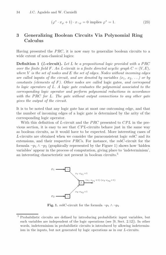
34 J.C. Agudelo and W. Carnielli
(ϕ∗ · xϕ + 1) · x¬ϕ = 0 implies ϕ∗ = 1. (23)
3 Generalizing Boolean Circuits Via Polynomial RingCalculus
Having presented the PRC, it is now easy to generalize boolean circuits to awide extent of non-classical logics:
Definition 1 (L-circuit). Let L be a propositional logic provided with a PRCover the finite field F . An L-circuit is a finite directed acyclic graph C = (V,E),where V is the set of nodes and E the set of edges. Nodes without incoming edgesare called inputs of the circuit, and are denoted by variables (x1, x2, . . .) or byconstants (elements of F ). Other nodes are called logic gates, and correspondto logic operators of L. A logic gate evaluates the polynomial associated to thecorresponding logic operator and perform polynomial reductions in accordancewith the PRC for L. The gate without output connections to any other gategives the output of the circuit.
It is to be noted that any logic gate has at most one outcoming edge, and thatthe number of incoming edges of a logic gate is determined by the arity of thecorresponding logic operator.
With this definition of L-circuit and the PRC presented to CPL in the pre-vious section, it is easy to see that CPL-circuits behave just in the same wayas boolean circuits, as it would have to be expected. More interesting cases ofL-circuits are obtained when we consider the paraconsistent logic mbC and itsextensions, and their respective PRCs. For instance, the mbC-circuit for theformula ¬p1 ∧ ¬p2 (graphically represented by the Figure 1) shows how ‘hiddenvariables’ appear in the process of computation, giving place to ‘indeterminism’,an interesting characteristic not present in boolean circuits.5
x1 �� ¬x1·xp1+1
�����
����
�
∧(x1·xp1+1)·(x2·xp2+1)
��
x2 �� ¬x2·xp2+1
����������
Fig. 1. mbC-circuit for the formula ¬p1 ∧ ¬p2
5 Probabilistic circuits are defined by introducing probabilistic input variables, butsuch variables are independent of the logic operations (see [9, Sect. 2.12]). In otherwords, indeterminism in probabilistic circuits is introduced by allowing indetermin-ism in the inputs, but not generated by logic operations as in our L-circuits.

Unconventional Models of Computation 35
This mbC-circuit, when variables x1 and x2 take both the value 0, producesthe output 1 in a deterministic way. But when x1 takes the value 1, the outputdepends on the hidden variable xp1 ; and when x2 takes the value 1, the outputdepends on the hidden variable xp2 . Hidden variables, like input variables, haveto take values in F (the field used in the PRC, in this case Z2), and we couldassume that values to hidden variables are randomly assigned. Then, we coulddistinguish between deterministic and non-deterministic L-circuits:
Definition 2 (Deterministic and non-deterministic L-circuit). An L-circuit is deterministic if the reduced polynomial of the output gate does notcontain hidden variables, otherwise the L-circuit is non-deterministic.
Note that there may be deterministic L-circuits with hidden variables withinthe circuit. For example, the mbC-circuit for the formula p1 ∨ ¬p1, graphicallyrepresented by the following figure:
x1 ��
�����
����
� ∨ 1 ��
¬x1·xp1+1
���������
Fig. 2. mbC-circuit for the formula p1 ∨ ¬p1
It is also important to take into account that non-deterministic L-circuitscould behave deterministically for some specific inputs, like the mbC-circuit forthe formula ¬p1 ∧ ¬p2 presented above.
Now, having defined the concept of L-circuit, it is opportune to discuss itspotentialities. Main characteristics of any model of computation concerns itscomputability power (the class of functions the model of computation can ex-press) and its computational complexity. Classically, it is possible to show thatto every boolean function whose inputs have a fixed length, there is a booleancircuit that computes such function (see for example [17, p. 79, prop. 4.3]).Non-computable functions arise when we consider functions whose inputs havearbitrary length. In this case it is necessary to define a family of circuits, whichis an infinite denumerable set of circuits {Ci}i∈N where the circuit Ci computesinputs of length i. To accept a family of circuits as an effective procedure wehave to impose the restriction that such a family of circuits should be uniformlygenerated, i.e. described by a Turing machine. Usually, uniform generation alsoimposes computational complexity restrictions; it establishes, for example, thatthe circuit must be generated by a polynomial time Turing machine, i.e. the timetaken to generate the circuit Ci must be a polynomial expression on i. A uni-formly generated family of circuits is called a uniform family of circuits. It canbe proven that uniform families of boolean circuits are equivalent (with respectto computability and computational complexity) to Turing machines (see [4]).
The next two sections explore potentialities of uniform families of L-circuitsas models of computation, first with respect to computability and then with

36 J.C. Agudelo and W. Carnielli
respect to computational complexity, considering only to the particular case ofparaconsistent logics.
3.1 Potentialities with Respect to Computability
Because paraconsistent logics are deductively weaker than CPL (or a version ofCPL in a different signature, see [7, Sect. 3.6]), we could think that the classof functions computed by uniform families of paraconsistent L-circuits would benarrower than functions computed by uniform families of boolean circuits, butwe will show that this is not the case for mbC.
Theorem 3. To every function computed by a uniform family of boolean circuitsthere is a uniform family of mbC-circuits that computes such function.
Proof. Let the mapping t1: For → For◦ (where For is the set or formulas ofCPL and For◦ is the set or formulas of mbC) defined as:
1. t1(p) = p, for any propositional variable p;2. t1(ϕ#ψ) = t1(ϕ)#t1(ψ), if # ∈ {∧,∨,→};3. t1(¬ϕ) =∼ t1(ϕ), where ∼ is defined in mbC as ∼ ϕ = ϕ→ (ψ∧ (¬ψ∧◦ψ)).
t1 conservatively translates CPL within mbC (cf. [7, p. 47]), that is, for everyΓ ∪ {ϕ} ⊆ For:
Γ �CPL ϕ iff t1(Γ ) �mbC t1(ϕ),
where t1(Γ ) = {t1(ψ) : ψ ∈ Γ}.Using t1, the uniform family of boolean circuits could be algorithmically trans-
lated to an equivalent uniform family ofmbC-circuits, just by changing the NOTgates for subcircuits corresponding to the formula ϕ→ (ψ ∧ (¬ψ ∧ ◦ψ)). It canbe checked that (ϕ→ (ψ∧ (¬ψ ∧◦ψ)))∗ = ϕ∗+1, which is the same polynomialas in classical negation. �The previous theorem can be generalized to several other paraconsistent logics,that is, to those where a conservatively translation function from CPL can bedefined taking into account that such translation function must be effectivelycalculated. In the other direction, the existence of uniform families of booleancircuits to every uniform family of L-circuits (for any logic L provided with PRC)is guaranteed by the classical computability of roots for polynomials over finitefields. Then, the L-circuits model does not invalidate Church-Turing’s thesis.
Generalizing PRC to infinite fields could be a way to define models of ‘hyper-computation’ (i.e. models that permit the computation of non Turing-machinecomputable functions, see [11]). For the case where the field is the rational num-bers with usual addition and multiplication, the output of a certain subclassof L-circuits would be Diophantine polynomials, and thus the problem of de-termining when L-circuits have 0 as output will be equivalent to the problemof determining when Diophantine equations have solutions, a well-known classi-cally unsolvable problem. However, in spite of the possibility of finding a cleverway (using hidden variables and polynomial operations) to determine 0 outputs

Unconventional Models of Computation 37
of L-circuits, hypercomputation would be attained at the cost of introducingan infinite element into the model, which seems to be opposed to the intuitiveidea of ‘computable’ (but most models of hypercomputation, nevertheless, areendowed with some kind of infinite element–see [12] and [13] for critiques ofhypercomputation).
3.2 Potentialities with Respect to Computational Complexity
Computational complexity potentialities can be thought in both directions too,that is: are there uniform families of boolean circuits more efficient than uniformfamilies of paraconsistent L-circuits? And vice versa? The first question has animmediate answer, but the other is not obvious. We will next show the answerto the first question, and subsequently some ideas related to the second.
Theorem 4. To every function computed by a polynomial size uniform familyof boolean circuits there is a polynomial size uniform family of mbC-circuits thatcomputes such function.
Proof. The translation t1, defined in the proof of Theorem 3 adds only a poly-nomial number of gates to the circuit (4 gates for every NOT gate). �As in the case of Theorem 3, Theorem 4 can be generalized to several otherparaconsistent logics, those to where a conservative translation function fromCPL can be defined (taking into account that such translation function must beeffectively calculated and add at most a linear number of gates to the circuits).
The other direction is left as an open problem, but we will show some analogiesbetween quantum circuits (see [8]) and paraconsistent circuits that could bevaluable in looking for a positive answer.
The quantum circuit model of computation is a generalization of the booleancircuits that depart from a quantum mechanics perspective. In a brief descriptionof such model of computation, we can say that classical bits are substitutedby qubits (or quantum bits). Qubits, in a similar way than classical bits, cantake values | 0 〉 and | 1 〉 (where | 0 〉 and | 1 〉 represent bases vectors in a twodimensional Hilbert space), but the radical difference is that qubits admit alsosuperpositions (or linear combinations) of such values, following the rules ofthe description of a quantum system in quantum mechanics. Superposition ofvalues are usually referred to as superposition states. In some interpretations ofquantum mechanics (as in the many-worlds interpretations), the states involvedin a superposition state are interpreted as coexisting, and then we can thinkthat qubits can take simultaneously the values | 0 〉 and | 1 〉, with probabilitiesassociated to each value. In quantum circuits, boolean gates are substitutedby quantum gates, which are unitary operators over qubits, also in agreementwith quantum mechanics. A relevant quantum gate is the so-called Hadamardgate, which transforms base states into perfect superposition states (states whereprobabilities are the same to any base state). Because quantum gates are alsolinear operators, the application of a gate to a superposition state is equivalent tothe simultaneous application of the gate to every base state in the superposition.

38 J.C. Agudelo and W. Carnielli
This characteristic allows the circuit to compute in parallel, in what is calledquantum parallelism. The problem is that when a measurement is performed,only one of the superposition states is obtained with a probability given bythe coefficients of the linear combination. Then, quantum algorithms must takeadvantage (before performing the measurement) of global characteristics of thefunctions computed in parallel.
We propose that outputs depending on hidden variables in L-circuits corre-spond to superposition states, since the indeterminism introduced by hiddenvariables allows us to simulate indeterminism of superposition states measure-ments. Under this assumption, gates corresponding to ¬ and ◦ in mbC andmbC+ logics, setting 1 as input, could be used to simulate the Hadamard gate(because in mbC, (¬ϕ)∗(1) = xϕ +1 and (◦ϕ)∗(1) = xϕ ·xϕ′ , and in mbC+ logicswe have that (◦ϕ)∗(1) = xϕ). To illustrate how ¬ and ◦ gates could be used inmbC-circuits and mbC+-circuits, we will demonstrate a relevant theorem:
Theorem 5. Let ϕ a formula in mbC and ϕ[pi/ψ] the formula obtained fromϕ by uniformly replacing pi by ψ. Then, ϕ∗ = f(x1, . . . , xi, . . . , xn) implies that(ϕ[pi/¬pi])∗(x1, . . . , 1, . . . , xn) = f(x1, . . . , xpi + 1, . . . , xn).
Proof. By induction on the complexity of ϕ. �Theorem 5 shows that, for mbC, by uniformly replacing in a formula ϕ thepropositional variable pi with the formula ¬pi, and setting 1 to the input variablexi in the corresponding mbC-circuit, we have that the output polynomial of thembC-circuit is equal to the polynomial for ϕ replacing the input variable xi withxpi + 1.
A similar theorem can be established formbC+ logics, uniformly replacing thepropositional variable pi with the formula ◦pi. In this case, the output polynomialis equal to the polynomial for ϕ replacing the input variable xi with the hiddenvariable xpi . This result could be used to compute satisfiability of CPL formulasin a non-deterministic way, taking the translation of a CPL formula to a mbC+
logic (with a conservative translation), by uniformly replacing all propositionalvariables pi with ◦pi and setting 1 to all input variables.
For example, the translation of the CPL formula ϕ = p1 ∧ p2 to a mbC+
formula (using the translation t1 above) is the same formula ϕ = p1 ∧ p2. Usingthe PRC for mbC, and the translation of ◦ϕ to polynomials in mbC+ logicsalready present above, we have that ϕ∗ = x1 ·x2 and (ϕ[p1/◦p1, p2/◦p2])∗(1, 1) =xp1 · xp2 . Note that the only thing we did was to replace input variables withhidden variables.
Obviously, for any CPL formula ϕwith propositional variables in {p1, . . . , pn},if ϕ is satisfiable, then (t1(ϕ)[p1/ ◦ p1, . . . , pn/ ◦ pn])∗(1, . . . , 1) = 1 for someassignment of values to hidden variables. An interesting question is whether thereexists any method, in accordance with PRC, that allows to eliminate hiddenvariables in such a way that polynomials distinct to the constant polynomial 0reduces to the constant polynomial 1. For some paraconsistent logics that wehave explored, this seems to be impossible, but we also do not have a definitenegative result (the possibility of polynomial conditions, see last paragraph of
Unconventional Models of Computation 39
Section 2, could be the key to obtain positive or negative results). We also haveto take into account that PRCs can be defined over distinct fields, and for other(not necessarily paraconsistent) non-standard logics.
4 Final Comments
This paper proposes a natural way to generalize boolean circuit model of com-putation to models based on non-standard logics. This opens possibilities tointegrate innovative concepts of non-standard logics into computational theory,shedding light into the question of how depending on logic abstract notions ofcomputability and algorithmic complexity could be. Moreover, the generaliza-tion proposed here has the advantage of being flexible enough to be almostimmediately adapted to a wide range of non-standard logics.
Cook’s theorem (cf. [10]) states that any NP-problem can be converted tothe satisfiability problem in CPL in polynomial time. The proof shows, in aconstructive way, how to translate a Turing machine into a set of CPL formu-las in such a way that the machine outputs ‘1’ if, and only if, the formulas areconsistent. As mentioned in the introduction, a model of paraconsistent Turingmachines presented in [1] was proved to solve Deutsch-Jozsa problem in an effi-cient way. We conjecture that a similar result as Cook’s theorem can be provento paraconsistent Turing machines. In this way, paraconsistent circuits couldbe shown to efficiently solve Deutsch-Jozsa problem. Consequences of this ap-proach would be the definition of ‘non-standard’ complexity classes relative tosuch unconventional models of computation founded over non-classical logics.
Finally, another relevant question that we do not tackle in this paper refers tophysical viability: are there any physical implementations to the hidden-variablemodel of computation presented here? We think that hidden-variable theories ofquantum mechanics (see [14]) could give a positive response to this question.
Acknowledgements
This research was supported by FAPESP- Fundao de Amparo Pesquisa doEstado de So Paulo, Brazil, Thematic Research Project grant 2004/14107-2.The first author was also supported by a FAPESP scholarship grant 05/05123-3,and the second by a CNPq (Brazil) Research Grant 300702/2005-1 and by anEU-FEDER grant via CLC (Portugal).
References
1. Agudelo, J.C., Carnielli, W.: Quantum algorithms, paraconsistent computation andDeutsch’s problem. In: Prasad, B. (ed.) Proceedings of the 2nd Indian InternationalConference on Artificial Intelligence, Pune, India, pp. 1609–1628 (2005)
2. Boolos, G., Jeffrey, R.: Computability and logic, 3rd edn. Cambridge UniversityPress, Cambridge (1989)

40 J.C. Agudelo and W. Carnielli
3. Richard Buchi, J.: Turing-machines and the Entscheidungsproblem. Mathematis-che Annalen 148, 201–213 (1962)
4. Calabro, C.: Turing Machine vs. RAM Machine vs. Circuits. Lecture notes, avail-able at http://http://www-cse.ucsd.edu/classes/fa06/cse200/ln2.ps
5. Coniglio Carlos Caleiro, M.E., Carnielli, W., Marcos, J.: Two’s company:the humbug of many logical values. In: Beziau, J.-Y. (ed.) Logica Univer-salis, pp. 169–189. Birkhauser Verlag, Basel, Switzerland (preprint available at)http://wslc.math.ist.utl.pt/ftp/pub/CaleiroC/05-CCCM-dyadic.pdf
6. Carnielli, W.A.: Polynomial ring calculus for many-valued logics. In: Werner, B.(ed.) Proceedings of the 35th International Symposium on Multiple-Valued Logic,pp. 20–25. IEEE Computer Society, Los Alamitos (2005), (preprint available atCLE e-Prints vol 5(3), 2005),http://www.cle.unicamp.br/e-prints/vol 5,n 3,2005.html
7. Carnielli, W.A., Coniglio, M.E., Marcos, J.: Logics of Formal Inconsistency. In:Gabbay, D., Guenthner, F. (eds.) Handbook of Philosophical Logic, 2nd edn.vol. 14, Kluwer Academic Publishers, Dordrecht (2005), (in print. preprint avail-able at CLE e-Prints vol 5(1), 2005),http://www.cle.unicamp.br/e-prints/vol 5,n 1,2005.html
8. Chuang, I.L., Nielsen, M.A.: Quantum Computation and Quantum Information.Cambridge University Press, Cambridge (2000)
9. Clote, P., Kranakis, E.: Boolean Functions and Computation Models. Springer,Heidelberg (2002)
10. Cook, S.A.: The complexity of theorem proving procedures. In: Proceedings of theThird Annual ACM Symposium on the Theory of Computing, pp. 151–158. ACMPress, New York (1971)
11. Copeland, J.: Hypercomputation. Minds and machines 12, 461–502 (2002)12. Davis, M.: The myth of hypercomputation. In: Teuscher, C. (ed.) Alan Turing: Life
and Legacy of a Great Thinker, pp. 195–212. Springer, Heidelberg (2004)13. Davis, M.: Why there is no such discipline as hypercomputation. Applied Mathe-
matics and Computation 178, 4–7 (2004)14. Genovese, M.: Research on hidden variable theories: A review of recent progresses.
Physics Reports 413, 319–396 (2005)15. Halpern, J.Y., Harper, R., Immerman, N., Kolaitis, P.G., Vardi, M.Y., Vianu, V.:
On the unusual effectiveness of logic in computer science. The Bulletin of SymbolicLogic 7(2), 213–236 (2001)
16. Jacobson, N.: Basic Algebra I, 2nd edn. W. H. Freeman and Company, New York(1985)
17. Papadimitriou, C.: Computational Complexity. Adisson-Wesley, London, UK(1994)
18. Turing, A.M.: On computable numbers, with an application to the Entschei-dungsproblem. In: Proceedings of the London Mathematical Society, pp. 230–265(1936) (A correction, ibid, vol 43, pp. 544–546, 1936-1937)

Amoeba-Based Nonequilibrium Neurocomputer
Utilizing Fluctuations and Instability
Masashi Aono and Masahiko Hara
Local Spatio-temporal Functions Lab., Frontier Research System,RIKEN (The Institute of Physical and Chemical Research),
Wako, Saitama 351-0198, [email protected]
Abstract. We employ a photosensitive amoeboid cell known as a modelorganism for studying cellular information processing, and construct anexperimental system for exploring the amoeba’s processing ability of in-formation on environmental light stimuli. The system enables to examinethe amoeba’s solvability of various problems imposed by an optical feed-back, as the feedback is implemented with a neural network algorithm.We discovered that the amoeba solves the problems by positively ex-ploiting fluctuations and instability of its components. Thus, our systemworks as a neurocomputer having flexible properties. The elucidation ofthe amoeba’s dynamics may lead to the development of unconventionalcomputing devices based on nonequilibrium media to utilize fluctuationsand instability.
Keywords: Bottom-up technology, Physarum, Optimization, Chaos.
1 Introduction
1.1 Fluctuations and Instability
Conventional computing devices are composed of rigid and stable materials topursue the accuracy and speed of their operations. Fluctuations and instabilityof the materials are negative disturbing factors that should be suppressed. Incontrast, biological systems perform information processing based on fluctuatedand unstable materials. Nevertheless, biological organisms succeed in survivingin harsh environments. They often demonstrate their ability to make flexible de-cisions and seek creative solutions to overcome critical situations. It is difficultfor conventional digital computers to demonstrate the flexibility and creativity.Exploring possible forms of processing based on fluctuated and unstable mate-rials, therefore, may lead to the development of flexible and creative computers.This expectation is one of our motives to carry out the study in this paper.
1.2 Nanotechnology for Next-Generation Device
Another motive is to tackle an issue faced by a specific field in nanotechnologyresearches, where the development of next-generation computing devices inte-grating a massive amount of molecular-scale components is one of immediate
S.G. Akl et al.(Eds.): UC 2007, LNCS 4618, pp. 41–54, 2007.c© Springer-Verlag Berlin Heidelberg 2007

42 M. Aono and M. Hara
priorities. Because it is extremely difficult to precisely manipulate all the com-ponents in a top-down manner, bottom-up approaches to utilize self-assemblingbehavior of the interacting components become increasingly important [1]. Atpresent, in most cases self-assembly is applied in fabrication processes of spatiallyordered structures of the components finally immobilized at static equilibrium.The next issue, remaining as an open question, is what to process with the fabri-cated structure, and how to make its components operate for the processing. Thetop-down manipulation of the components would be difficult here again. There-fore, it is necessary to explore potentials of processing realizable in a bottom-upmanner.
1.3 Self-organization in Nonequilibrium Media
On the other hand, in a field studying nonlinear dynamic systems, there areseveral proposals to create processing units using self-organized spatiotemporalpatterns of chemical components at dynamic nonequilibrium [2]. Some oscilla-tory or excitable chemical media, such as the Belousov-Zhabotinsky reactionsystem, generate reaction-diffusion waves. The propagating wave transfers infor-mation (for example an ON-state signal) from one site to another. Based on thecontrol of the passage, collision, coincident initiation and annihilation of multiplepropagating waves at particular sites, some authors have experimentally demon-strated various processing units, such as a maze solver [3] and logical operators[4]. There is a view that this form of processing gives an extremely simplifiedmodel of information processing performed in biological cells.
In this form of processing, the fluctuations and instability in chemical mediaare vital for providing the background for processing. The randomness drivingcollisions of reactants is responsible for chemical reactions, and the unstablereaction dynamics is necessary for producing the spatiotemporal patterns. How-ever, unless the fluctuations and instability are kept at a moderate level, theybecome negative disturbing factors, just as they are suppressed in conventionaldevices. Indeed, because the coincidence of multiple propagating events is cru-cial for ensuring the accuracy of processing results, the timing and orbit ofthe wave propagation should not be fluctuated and destabilized. Some form oftop-down precise control of the propagating events is needed for ensuring theaccuracy, but it might undermine the significance of utilizing the bottom-upbehavior.
The basic principle of the above proposals, that operations of processing unitsshould be accurate and stable, is essentially identical with that of conventionaldevices. It is necessary to dilute this basic principle for exploring potentialsof processing that utilize the bottom-up behavior involving fluctuations andinstability. We take a heuristic approach to discover a novel form of processingwhose principle is unknown. That is, first we construct a device using a specificmedium, and then try to find out what kind of processing would be the mostappropriate for the medium. In this paper, we employ a unicellular amoeboidorganism that is a kind of biological oscillatory media. As explained in the nextsection, the amoeba is one of the most suitable organisms for our study.

Amoeba-Based Nonequilibrium Neurocomputer 43
Fig. 1. (A) A huge individual of unicellular amoeba (scale bar=5mm). (B) Au-coatedplastic barrier structure on agar plate without nutrients (scale bar=2 mm). The amoebaacts only inside the structure where agar is exposed, as it averts the metal surface. Ini-tial configuration < 0, 0, 0, 0, 0, 0, 0, 0 > is input by placing the amoeba at the center.(C) Schematic of the body structure. (D) Schematic of the contraction-relaxation ofactomyosins. (E) The occurrence of rapid expansion/shrinkage of a branch vs. the os-cillation phase difference between the branch and hub part. Results for rapid shrinkageare shown upside down.
2 Materials and Methods
2.1 True Slime Mold
An amoeba of true slime mold Physarum polycephalum is a huge multinucleatedunicellular organism (Fig. 1A). In order to evaluate the amoeba’s processing abil-ity by its rationality of the shape deformation, we confine an individual amoebawithin the stellate barrier structure put on an agar plate (Fig. 1B). The amoebaconcurrently expands or shrinks its multiple branches inside the structure. Weemployed the amoeba because it has favorable features in its structure and func-tion that fit for our purpose.
Body Structure. The amoeba’s body structure is extremely simple and ho-mogeneous. Fig. 1C schematically shows the structure of when there are threeexpanding branches. An individual amoeba has only a single gel layer (a sortof cellular membrane) enveloping intracellular sol. The gel layer is formed by amassive amount of actomyosins (fibrous proteins contained in muscle) capableof taking contracting or relaxing states (Fig. 1D). These actomyosins are thedriver elements of the amoeba, as they play a major role in the shape deforma-tion. Because numerous cell nuclei are distributed throughout the homogeneousbody of an individual amoeba, a part of the amoeba divided from the individualsurvives as another self-sustainable individual. Conversely, multiple individualsfuse together to form an individual when they are contacted. The simplicityand homogeneity of the structure would make the elucidation of the amoeba’sdynamics comparatively easy.

44 M. Aono and M. Hara
Oscillation. The gel layer has a sponge-like property in which extruding andabsorbing of intracellular sol is driven by the contraction and relaxation ofcrosslinked actomyosins at a local site, respectively. Collectively entrained ac-tomyosins generate rhythmic contraction-relaxation cycle observed as verticalthickness oscillation of the gel layer (period=1 ∼ 2 min) with various spa-tiotemporal patterns, where its physiological mechanism has not been eluci-dated completely. As the phase of the oscillation varies from site to site, in-tracellular sol is forced to stream horizontally (velocity=∼ 1 mm/sec) by thepressure difference (gradient) derived from the contraction tension difference ofthe gel layer. The oscillation induces the iterations of direction reversals of thesol streaming in a shuttlewise manner. Intracellular substances including acto-myosins and various chemicals essential for the contraction-relaxation oscillation(e.g. Ca2+ and ATP ) are transported by the sol to travel throughout the wholebody.
Deformation. A branch expands or shrinks at a velocity of at most 1 cm/h, asthe shuttlewise sol efflux-influx for the branch is iterated for several periods ofthe oscillation. During our experiment, the amoeba deforms its shape withoutchanging its total volume by keeping a nearly constant amount of intracellularsol. Fig. 1E shows the occurrence rate of rapid expansion/shrinkage of a branchas a function of the oscillation phase difference between the branch and the hubpart. When a branch expands rapidly, it is notable that the branch and thehub part synchronize in antiphase (i.e., phase difference � 180◦). Conversely, in-phase synchronization (i.e., phase difference � 0◦) cannot yield rapid expansion.The velocity of shrinkage was lower than that of expansion, and no significantcorrelation with the phase difference was confirmed. These results suggest that;i) a branch expands rapidly when its relaxing gel layer invites a greater influx ofthe sol extruded by the contracting gel layer of the hub part (Fig. 1C), and ii) theshrinkage of a branch is driven passively as the sol flows out to other expandingbranches. Namely, the amoeba’s decision on its horizontal shape deformation ismade by spatiotemporal patterns of vertical thickness oscillation [5].
Optimization Capability. Despite the absence of a central system, theamoeba exhibits sophisticated computational capacities in its shape deforma-tion. Indeed, the amoeba is capable of searching for a solution of a maze [6].Inside a barrier structure patterned to have walls of the maze, the amoeba de-forms its shape into a string-like configuration that is the shortest connectionpath between two food sources at the entrance and exit of the maze. This resultshows that the amoeba realizes the optimization of the nutrient absorption ef-ficiency and leads its whole body to a favorable condition for the survival. Theamoeba’s shape deformation is handled by spatiotemporal oscillation patterns.The spatiotemporal pattern is self-organized by collectively interacting acto-myosins. Therefore, the amoeba can be regarded as a sophisticated informationprocessor utilizing the bottom-up behavior of massively parallel components.This feature fits for exploring potentials of processing realizable with nonequi-librium media in a bottom-up manner.

Amoeba-Based Nonequilibrium Neurocomputer 45
B
C
VCPJ
PC
SM
LS
A neuron i : inactive
amoeba
neuron i : active
light onamoeba
light oni+1i-1
X-shaped Y-shaped
Fig. 2. (A) Optical feedback system. For transmitted light imaging using a video cam-era (VC), the sample circuit (SM) was illuminated from beneath with a surface lightsource (LS). The recorded image was processed using a PC to update the monochromeimage for illumination with a projector (PJ). (B) Optical feedback rule: active statexi(t) = 1 triggers light illumination yi−1(t + Δt) = yi+1(t + Δt) = 1 (white lightprojected to rectangular regions). (C) All possible solutions of the problem.
2.2 Neural Network Implementation
State of Neuron. We call the i th path of the stellate structure “neuron i”(i ∈ I = {1, 2, · · · , N = 8}). The amoeba’s shape is monitored using a videocamera at each interval of Δt = 6 sec (Fig. 2A). For each neuron i at time t,whenever more than a quarter of the area of the i th neuron is occupied by theamoeba’s branch, state 1 (active) is assigned as xi(t) = 1, otherwise xi(t) = 0(inactive). The amoeba’s shape is freely deformable to fit into arbitrary boundarycondition of any network topology. Thus, the computing can be started fromarbitrary input configuration < x1(0), x2(0), · · · , xN (0) >.
Photoavoidance-Based Control. The amoeba’s branch exhibits photoavoid-ance response. A branch is shrunk by a local light stimulation, as the light-induced contraction enhancement of the gel layer intensifies the sol efflux (ex-trusion) from the stimulated region [7]. A neuron, therefore, is led to be inactiveby illuminating the corresponding region. The illumination is carried out with aprojection of a monochrome image such that only the regions to be illuminatedare colored in white (Fig. 2A). We write yi = 1 if the light for the neuron iis turned on. Conversely, if the neuron i is allowed to be xi = 1, the light isturned off as yi = 0. Any neuron is activated naturally if it is not illuminated,because the amoeba inherently tries to expand all branches to generate the con-figuration < 1, 1, 1, 1, 1, 1, 1, 1 >. The illumination pattern < y1, y2, · · · , yN >,therefore, leads the system configuration < x1, x2, · · · , xN > toward the idealconfiguration < x′1, x
′2, · · · , x′N > such that all neurons satisfy the follwing con-
dition: x′i = 1 − yi. We call this condition “counteractive rule” and adopt it asour system’s control principle.

46 M. Aono and M. Hara
Feedback Dynamics. In assuming the counteractive rule, the optical feedbacksystem automatically updates the illumination pattern. The feedback is imple-mented with a discrete form of recurrent neural network dynamics known asHopfield-Tank model [8]: yi(t + Δt) = 1 − f(ΣN
j=1wijxj(t)), where wij is theweight assigned to the link from the neuron j to neuron i, and the thresholdθ = 0 defines the step function f(σ) = 1 if σ ≥ θ, otherwise 0. The illuminationpattern is updated at each interval with the change in the system configuration,and again it induces further deformation of the amoeba.
Stable Equilibrium Solution. Any configuration is called “stable equilib-rium” if and only if the counteractive rule is satisfied for all neurons. In a stableequilibrium, the amoeba is no longer forced to reshape by illumination and canfully expand its branches inside all nonilluminated neurons. Thus, the configu-ration would be comfortable for the amoeba, and is expected to be stably main-tained unless the amoeba spontaneously breaks the counteractive rule. In theformalization of the recurrent neural network, a stable equilibrium is regardedas a solution of the problem defined by assigning the weights. In general, thereexist multiple solutions, and each solution has minimum energy of the potentialenergy landscape established by the network dynamics. Any medium that canonly relax toward its stable equilibrium, therefore, cannot bootstrap itself out ofa once-reached solution having locally minimum energy.
2.3 Embodiment of Problem Solving
Constraint Satisfaction Problem. We assigned the weights as wij = −1 if|i− j| = 1, otherwise 0, to define the following symmetric rule for updating theillumination (Fig. 2B): If the neuron i is active (xi(t) = 1), its adjacent neuronsi − 1 and i + 1 are induced to be inactive by illumination (yi−1(t + Δt) =yi+1(t+Δt) = 1), where the boundary condition is periodic. This rule prohibitstwo adjacent neurons i and i+1 from taking active state simultaneously. Anotherinterpretation of this rule is that each neuron is led to execute logical NOR-operation known as a universal logic element: The neuron i is illuminated to beinactive (xi(t+Δt) = 0), if at least one of its adjacent neurons is active (xi−1(t) =1 or xi+1(t) = 1), otherwise (xi−1(t) = xi+1(t) = 0) nonilluminated to be active(xi(t+Δt) = 1). Namely, the optical feedback imposes the following constraintsatisfaction problem: Find the system configuration < x1, x2, · · · , x8 > suchthat all neurons satisfy xi = NOR(xi−1, xi+1). As a solution of this problem,the amoeba is required to search for a stable equilibrium. There are 10 solutions(Fig. 2C) consisting of rotation symmetric groups of < 1, 0, 1, 0, 1, 0, 1, 0> (“X-shaped”) and < 1, 0, 0, 1, 0, 0, 1, 0 > (“Y-shaped”).
Livelock and Deadlock. The concurrent processing of circularly connectedNOR-operators has a potential of creating a stalemated unsolvability of theproblem, when all operations are executed in a synchronous manner. Let us sup-pose that all branches expand or shrink with a uniform velocity. From the initialconfiguration < 0, 0, 0, 0, 0, 0, 0, 0 > evoking no illumination, the synchronous

Amoeba-Based Nonequilibrium Neurocomputer 47
expanding movements of all branches will lead to < 1, 1, 1, 1, 1, 1, 1, 1 >. In thisconfiguration, all neurons are illuminated. Then, all branches shall shrink uni-formly to evacuate from the illuminations. This leads all branches to return tothe initial configuration that allows them to expand again. In this manner, thesystem can never attain a solution, as the synchronous movements result in aperpetual oscillation between < 0, 0, 0, 0, 0, 0, 0, 0 > and < 1, 1, 1, 1, 1, 1, 1, 1 >.This type of stalemated situation is called “livelock”.
On the other hand, let us assume that the problem could be solved success-fully. The amoeba is expected to stably maintain the solution because it wouldbe a temporarily comfortable condition. However, the amoeba would inherentlyintend to search for foods by the deformation with the expanding behavior ofbranches. Permanently maintaining the solution, therefore, eliminates any pos-sibility of feeding and brings about its death from starvation1. This is anothertype of stalemated situation resembling “deadlock”. Thus, our experiment re-quests the achievement of the following two goals to the amoeba; the amoebashould be capable of not only livelock avoidance for attaining a solution, but alsodeadlock avoidance for breaking away from the solution [9,10,11]. We carried outthe experiment to observe how the amoeba copes with the stalemated situationsin a bottom-up manner.
3 Results
3.1 Problem Solving Process
Spatiotemporal Oscillation Pattern. The experiment was started from theinitial configuration < 0, 0, 0, 0, 0, 0, 0, 0 > (Fig. 1B) by placing the amoeba’sspherical piece (0.75±0.05 mg) at the center of the stellate structure. In the earlystage, the amoeba flattened its spherical shape to turn into disc-like shape, andhorizontally expanded its thin periphery in a circularly symmetric manner. Asshown in panels of Fig. 3, by binarizing the phase of vertical thickness oscillationof each local site into increasing (relaxing) and decreasing (contracting) phases,we can clearly observe spatiotemporal oscillation patterns.
Spontaneous Symmetry-Breaking. The amoeba’s circular deformation (i.e.,synchronous expanding movements of all branches) would be inevitable if realiz-able spatiotemporal patterns were limited to circularly symmetric ones. However,we observed that the amoeba produces various symmetry-broken patterns, andthe pattern varies nonperiodically in a complex manner. As shown in Fig. 3A,the symmetry was spontaneously broken as a defective site was created in theperiphery. The defective site was exclusively expanded at a velocity relativelylarger than that of the rest, and developed into a distinct branch having enoughoccupying area inside the neuron 8 to evoke the illumination.1 Although no food source is given in our experimental condition, the amoeba in our
experiment can survive without any food for up to about a week because it can storenutrients fed before the experiment as internal energy source.

48 M. Aono and M. Hara
Fig. 3. Time course of events in computing process. (A) Transient configuration< 0, 0, 0, 0, 0, 0, 0, 1 >. Illuminated regions are indicated by rectangles. The oscilla-tion phase is binarized into the relaxing (thickness increasing) and contracting (de-creasing) states, represented by the black (red in colored version) and gray (blue)pixels, respectively. (B) First-reached solution < 0, 1, 0, 0, 1, 0, 0, 1 > (duration�4h). (C) Spontaneous destabilization. The solution B < 0, 1, 0, 0, 1, 0, 0, 1 > (left)evolved into < 0, 1, 1, 0, 1, 0, 1, 1 > (right). Arrows indicate the growth directions ofthe newly emerged branches expanding under illumination contrary to photoavoid-ance. (D) Second-reached solution < 0, 1, 0, 0, 1, 0, 1, 0 > (duration�1 h). (E) Spon-taneous destabilization. The solution D < 0, 1, 0, 0, 1, 0, 1, 0 > (left) evolved into< 0, 1, 0, 0, 1, 0, 1, 1 > (right). (F) Third-reached solution < 0, 1, 0, 1, 0, 1, 0, 1 >(duration�7 h).
Solution Seeking with Livelock-Breaking. Sometimes we observe thelivelock-like situation in which the amoeba’s circularly symmetric deformationcontinues by keeping its disc-like shape until all neurons are illuminated. Evenin that case, the symmetry is spontaneously broken and movements of pe-ripheral parts become asynchronously fluctuated with mutual time lags. Ow-ing to the asynchronously fluctuated movements, the livelock-like stalemate wasavoided, and the amoeba searched for the solution< 0, 1, 0, 0, 1, 0, 0, 1> shown inFig. 3B. The solution was stably maintained for about 4 h. We observed thatthe spatiotemporal pattern of vertical oscillation evolves nonperiodically whilethe amoeba’s shape in the solution is unchanged horizontally [12,13,14].
3.2 Searching Ability of Multiple Solutions
Destabilization of Solution with Deadlock-Breaking. The stabilizationof the solution (Fig. 3B) was longly persisted as if the amoeba is stalematedin a deadlock-like situation. However, the stabilizing mode was spontaneouslyswitched to the destabilizing mode without any explicit external perturbation.

Amoeba-Based Nonequilibrium Neurocomputer 49
Interestingly, the amoeba broke through the deadlock, as two branches suddenlyemerged and started to invade illuminated regions (Fig. 3C). The invading be-havior against the counteractive rule is contrary to the photoavoidance response.
Spontaneous Switching between Stabilizing and Destabilizing Modes.While aggressive expansion of the branch 7 was sustained under illumination,the branch 8 was shrunk by illumination. In this manner, the branches iteratedtheir asynchronously fluctuated movements again. As a result, the amoeba suc-ceeded in searching for another solution < 0, 1, 0, 0, 1, 0, 1, 0 > (Fig. 3D). Thenamoeba stabilized its shape at the second solution for about 1 h. After that,the spontaneous destabilization occurred once more (Fig. 3E), and eventuallythe amoeba attained the third solution < 0, 1, 0, 1, 0, 1, 0, 1 > maintained forabout 7 h (Fig. 3F). Within 16 h of the observation, the amoeba successivelysearched for three solutions by repeatedly switching between the stabilizing anddestabilizing modes.
3.3 Statistical Results
We carried out 20 experimental trials measured for an average of 14.5 h. As shownin Fig. 4A, in every trial at least one solution was searched, and transition amongan average of 3.25 solutions (gross number including multiple attainments of anidentical solution) was realized per a trial. This result implies that the amoebasignificantly has the capabilities of searching for solutions and destabilizing thesolutions.
The transition among solutions was observed as nonperiodic. As shown inFig. 4B, the duration of a solution distributes within a range of about 0.5 hto 12 h. The durations of X-shaped solutions are relatively longer than that ofY-shaped ones. This suggests that X-shaped solutions are more stable than Y-shaped ones. The transition is stochastic in a sense that a solution has a potentialto evolve into multiple solutions. We confirmed that transition from more stableX-shaped solution to less stable Y-shaped one is possible.
Fig. 4. Statistical results. All data were obtained from 20 trials. (A) Frequency distri-bution of the number of solutions searched. (B) Frequency distribution of the durationtime of stay in a solution. Results were evaluated separately for X-shaped and Y-shapedsolutions, and are shown in a stacked manner (e.g., Y-shaped ones maintained for therange of 0.5 to 1 h were observed 13 times).

50 M. Aono and M. Hara
4 Discussions
4.1 Biological Implication of Spontaneous Destabilization
In the stabilizing mode, all branches keep away from illumination for maintain-ing a solution. In the destabilizing mode, under equal illumination conditions,some branches enterprisingly invade aversive illuminated regions contrary totheir photoavoidance, while others remain shrunk as usual. This implies thatthe amoeba’s photoavoidance response is nonuniform spatially and temporally.This flexibly variable stimulus-response would be essential for the survival of theamoeba required to search for food in a harsh environment, because it enablesthe amoeba surrounded by aversive stimuli to break through the stalemated sit-uation with enterprising responses. In our experiment, the deadlock-like criticalsituation in which the amoeba is stuck in its starved condition was flexibly bro-ken by the amoeba’s spontaneous destabilization. That is, unstable phenomenahave a positive aspect to produce the flexibility.
4.2 Mechanism of Emergence of New Branch
The spontaneous destabilization is realized as new branches emerge suddenly,although its mechanism remains to be seen. In most cases, a new branch emergesas a singularly thick structure with localized large vertical oscillation amplitude.It appears to intensively invite a drastic sol influx from a broad domain. Figure 5illustrates our speculation that the singularly thick structure is formed as intra-cellular sol spouts vertically from the gel layer’s defective site where it is locallyfragile to be ruptured (i.e., crosslinking of actomyosins is broken). According tothis assumption, the structure of the newly emerged branch is composed chieflyof extruded sol and is not covered by a sufficient quantity of gel to actualizelight-induced contraction. Such a soft blob-like structure must be incapable ofphotoavoidance response, and thus it can be extruded to expand flexibly evenunder unfavorable illuminated conditions. Fragile and unstable components ofbiological systems may provide a positive aspect to enable flexible behavior.
Fig. 5. Schematic of speculated process in the emergence of a new branch. A fragiledefect of the gel layer is ruptured, and a new branch is formed as the sol spouts fromthe defect. The branch rapidly develops through self-repairing process of the defect.
Amoeba-Based Nonequilibrium Neurocomputer 51
4.3 Origin of Spontaneous Destabilization
The spontaneous switching between the stabilizing and destabilizing modes ( i.e.,the transition among solutions) was observed as nonperiodic and stochastic. Asone of its possible origins, we suppose the combination of intrinsic microscopicfluctuations and spatiotemporal chaos characterized as nonperiodic but nonran-dom behavior. Indeed, the system’s behavior is chaotic as its time evolution isunstable and unreproducible. Its capability of successively searching for multiplesolutions, however, is robustly maintained and qualitatively reproducible. Thisresembles the robustness of strange attractors of chaotic systems.
Unstable chaotic dynamics with properly tuned parameter intermittentlyswitches between the stabilizing and destabilizing modes by exponentially am-plifying microscopic fluctuations [15]. That is, fluctuations in the microscopiclevel such as the thermal noise, nonuniformity of chemical distributions, and thegel layer’s uneven stiffness distribution (density distribution of crosslinked acto-myosins), are amplified to an extensive and sustained movements of the macro-scopic level. Some form of positive feedback effect by the coupling of chemical,physiological, and hydrodynamic processes may be responsible for the amplifi-cation process.
4.4 Applications
Logical Circuit, Associative Memory, and Optimization ProblemSolver. The amoeba’s capability to search for a stable equilibrium under ouroptical feedback allows our system to be developed to a logical circuit holdinga kind of computational universality. By properly altering the system parame-ters including the number of neurons, thresholds, and weights, our system canimplement a network of the McCulloch-Pitts neurons capable of simulating anyBoolean logic operations with the network architecture allowing arbitrary circuitwiring [16]. In addition, the system can be developed to an associative memorydevice by regarding a stable equilibrium as a predefined memory pattern.
Moreover, the amoeba’s capability of transition among multiple stable equilib-ria may fit for solving combinatorial optimization problem (e.g. traveling sales-man problem), because it may assist searching for a global optimum solutionwithout being stuck at local optima. The usefulness of chaotic dynamics for com-binatorial optimization has already been clarified with chaotic neural networkmodels, where both stabilizing and destabilizing effects contribute to efficientsearching dynamics [17,18].
Future Perspective on Flexible Device. In the conventional computingparadigm, deadlock can be avoided in the software level, if it is possible toprescribe an appropriate resource allocation protocol comprehending potentialresource requests from all processes. However, no programmer can know whatthe processes will request in advance of the coding without actual executions.This means that deadlock avoidance is often impossible for many practical sys-tems. On the other hand, our system flexibly breaks through the livelock-like

52 M. Aono and M. Hara
and deadlock-like situations and searches for several solutions without provid-ing any particular resource allocation protocol. This is because the amoeba’sspatiotemporal oscillation patterns autonomously materialize and alter the allo-cation of intracellular sol to its branches in a bottom-up manner. In contrast tothe conventional paradigm based on hardwares operating passively as instructedby software programs, the amoeba as a hardware in our system actively altersthe interpretation of the software program (i.e., the control principle with thefeedback algorithm). This unique capability would be advantageous in the devel-opment of autonomous systems operated in actual environments, such as robotcontrol systems [19]. It may enable the robot to flexibly respond to concurrentoccurrences of unexpected events that would lead the robot to stalemated situ-ations, even if the programs prescribed only for expected events were defectiveor useless for searching for solutions to overcome the situations.
Although dramatic improvement in its slow processing speed is unpromisingas long as the amoeba is used, it may be possible to develop our computingscheme by implementing with other faster materials, if the dynamics of theamoeba’s oscillatory behavior is elucidated. Potential candidates suitable as thealternative materials would be oscillatory or excitable nonequilibrium mediacapable of spontaneously breaking the spatiotemporal symmetries in a chaoticmanner.
5 Conclusions
Our discoveries and discussions in this paper are summarized as follows.
1. Fluctuations and instability in the amoeba’s components have positive as-pects to produce the enhancement of searching ability and the flexibility ofdecision-making ability.– The amoeba is capable of searching for a stable equilibrium solution
of a constraint satisfaction problem, due to its ability to fluctuate itsmovements for breaking through a livelock-like stalemated situation.
– The amoeba is capable of searching for multiple solutions one after an-other by spontaneously destabilizing once-reached solutions, because ithas flexibility to change its stimulus-response for breaking through adeadlock-like stalemated situation.
2. The above problem solving is realizable owing to the amoeba’s rebelliousbehavior against the feedback control, and it presents a possible form ofprocessing to utilize the bottom-up behavior of fluctuated and unstablematerials.
3. The amoeba’s searching ability and flexibility allow our system to be devel-oped to logical circuits, associative memory devices, combinatorial optimiza-tion problem solvers, and novel devices that flexibly respond to occurrencesof unexpected events.
4. If the amoeba’s oscillatory dynamics is elucidated, our proposal may beimplementable by other faster nonequilibrium medium.

Amoeba-Based Nonequilibrium Neurocomputer 53
References
1. Whitesides, G.M., Grzybowski, B.A.: Self-Assembly at all Scales. Science 295,2418–2421 (2002)
2. Adamatzky, A., De Lacy Costello, B., Asai, T.: Reaction-Diffusion Computers.Elsevier, UK (2005)
3. Steinbock, O., Toth, A., Showalter, K.: Navigating Complex Labyrinths: OptimalPaths from Chemical Waves. Science 267, 868–871 (1995)
4. Motoike, I., Yoshikawa, K.: Information operations with an excitable field. Phys.Rev. E 59, 5354–5360 (1999)
5. Nakagaki, T., Yamada, H., Ueda, T.: Interaction between cell shape and contractionpattern. Biophys. Chem. 84, 195–204 (2000)
6. Nakagaki, T., Yamada, H., Toth, A.: Maze-solving by an amoeboid organism. Na-ture 407, 470 (2000)
7. Ueda, T., Mori, Y., Nakagaki, T., Kobatake, Y.: Action spectra for superoxidegeneration and UV and visible light photoavoidance in plasmodia of Physarumpolycephalum. Photochem. Photobiol. 48, 705–709 (1988)
8. Hopfield, J.J., Tank, D.W.: Computing with neural circuits: A model. Science 233,625–633 (1986)
9. Aono, M., Gunji, Y.P.: Beyond input-output computings: Error-driven emergencewith parallel non-distributed slime mold computer. BioSystems 71, 257–287 (2003)
10. Aono, M., Gunji, Y.P.: Resolution of infinite-loop in hyperincursive and nonlo-cal cellular automata: Introduction to slime mold computing. In: Dubois, D.M.(ed.) Computing Anticipatory Systems: CASYS 2003. AIP conference proceedings,vol. 718, pp. 177–187 (2004)
11. Aono, M., Gunji, Y.P.: Material implementation of hyperincursive field on slimemold computer. In: Dubois, D.M. (ed.) Computing Anticipatory Systems: CASYS2003. AIP conference proceedings, vol. 718, pp. 188–203 (2004)
12. Takamatsu, A., et al.: Time delay effect in a living coupled oscillator system withthe plasmodium of Physarum polycephalum. Phys. Rev. Lett. 85, 2026 (2000)
13. Takamatsu, A., et al.: Spatiotemporal symmetry in rings of coupled biologicaloscillators of Physarum plasmodial slime mold. Phys. Rev. Lett. 87, 078102 (2001)
14. Takamatsu, A.: Spontaneous switching among multiple spatio-temporal patternsin three-oscillator systems constructed with oscillatory cells of true slime mold.Physica D 223, 180–188 (2006)
15. Kaneko, K., Tsuda, I.: Complex Systems: Chaos and Beyond - A ConstructiveApproach with Applications in Life Sciences. Springer, New York (2001)
16. Arbib, M.A. (ed.): The Handbook of Brain Theory and Neural Networks. The MITPress, Cambridge, Massachusetts (2003)
17. Aihara, K., Takabe, T., Toyoda, M.: Chaotic Neural Networks. Phys. Lett. A 144,333–340 (1990)
18. Hasegawa, M., Ikeguchi, T., Aihara, K.: Combination of Chaotic Neurodynam-ics with the 2-opt Algorithm to Solve Traveling Salesman Problems. Phys. Rev.Lett. 79, 2344–2347 (1997)
19. Tsuda, S., Zauner, K.P., Gunji, Y.P.: Robot Control with Biological Cells. In:Proceedings of Sixth International Workshop on Information Processing in Cellsand Tissues, pp. 202–216 (2005)

54 M. Aono and M. Hara
Appendix
Experimental Setups
The amoeba was fed by oat flakes (Quaker Oats, Snow Brand Co.) on a 1% agargel at 25◦C in the dark. The stellate barrier structure (thickness approximately0.2 mm) is made from an ultrathick photoresist resin (NANOTM XP SU-8 3050,MicroChem Corp.) by a photolithography technique, and was coated with Auusing a magnetron sputter (MSP-10, Shinkuu Device Co., Ltd.). The experi-ments were conducted in a dark thermostat and humidistat chamber (27±0.3◦C, relative humidity 96±1%, THG062PA, Advantec Toyo Kaisha, Ltd.). Fortransmitted light imaging, the sample was placed on a surface light guide (MM80-1500, Sigma Koki Co., Ltd.) connected to a halogen lamp light source (PHL-150, Sigma Koki Co., Ltd.) equipped with a band-pass filter (46159-F, EdmundOptics Inc.), which was illuminated with light (intensity 2 μW/mm2) at a wave-length of 600±10 nm, under which no influence on the amoeba’s behavior wasreported (Ueda et al., 1988). The intensity of the white light (monochrome colorR255:G255:B255) illuminated from the projector (3000 lm, contrast ratio 2000:1,U5-232, PLUS Vision Corp.) was 123 μW/mm2. The outer edge of the circuit(border between the structure and the agar region) was always illuminated toprevent the amoeba from moving beyond the edge.
Unconventional “Stateless” Turing–Like
Machines
Joshua J. Arulanandham
School of Computing SciencesVIT University, Vellore, India
Abstract. We refer to Turing machines (TMs) with only one state as“stateless” TMs. These machines remain in the same state throughoutthe computation. The only way they can “remember” anything is bywriting on their tapes. Stateless TMs have limited computing power:They cannot compute all computable functions. However, this handicapof a stateless TM can be overcome if we modify the TM a little byadding an extra feature. We propose a modified Turing–like machinecalled a JTM—it is stateless (has only one internal state) by definition—and show that it is as powerful as any TM. That is, a JTM does notswitch states, and yet can compute all computable functions. JTMs differfrom conventional TMs in the following way: The tape head spans threeconsecutive cells on the tape; it can read/write a string of three (tape)symbols all at once. However, the movement of the head is not in termsof “blocks of three cells”: in the next move, the head does not “jump”to the adjacent (entirely new) block of three cells; it only shifts itself byone cell—to the right or to the left. A JTM is more than a product oftheoretical curiosity: it can serve as a “normal form” and might lead tosimpler proofs for certain theorems in computation theory.
1 Turing Machines
Turing machines (TMs), proposed by Alan Turing [2] in 1936, are one of thefirst “toy models” that were used to define precisely the notions of computa-tion and computability—what it means to “compute”, and what can and cannotbe computed. A TM is actually a simple mechanical device that does symbol–manipulation (which one can actually build, if one wants to!), but is often em-ployed as a “paper machine”, i.e. as a theoretical construct in computer science.Theorems regarding the nature of computation proven using TMs apply to realcomputers, since TMs faithfully model real computers, i.e. any input–outputfunction computable on a digital computer can be computed on a TM [1]. Inwhat follows we first give an informal description of the Turing machine, andthen, some formal definitions.
The Turing machine has a tape that is divided into cells (squares); the tapeextends infinitely to the right and to the left. Each cell of the tape can hold asymbol. The tape initially contains the input—a finite string of symbols in the
S.G. Akl et al.(Eds.): UC 2007, LNCS 4618, pp. 55–61, 2007.c© Springer-Verlag Berlin Heidelberg 2007

56 J.J. Arulanandham
input alphabet—and is also used to hold the output, once the computation isover. Cells other than those containing the input are initially “blank”, i.e. theyhold the special (blank) symbol B. “Computation” on a TM is accomplished byreading and (over)writing symbols on the tape: There is a tape head (initiallypositioned over the left most symbol of the input) that hops from cell to cell,reading and writing a symbol. The tape head (its movement, read/write process)is controlled by a control unit that can switch between different states (a finiteset), each of which represents a certain “mode of operation”1. Each move of aTM depends on two things: the state of the control unit and the symbol beingread (scanned) by the tape head. In one move, a TM will: (i) Write a (possibly,new) symbol on the cell under the tape head, (ii) Shift the tape head one cell,to the left or to the right and, (iii) Update the state of the control unit, possiblychanging it to a new state.
Definition 1. A TM can be described as a 6–tuple M = (Q,Σ, Γ, δ, q0, B) whereQ is the finite set of states of the control unit, Σ is the finite set of inputsymbols, Γ is the set of tape symbols (Σ is a proper subset of Γ ), δ : Q× Γ →Q×Γ ×{L,R} is the transition function, q0 ∈ Q is the start state of the controlunit, and B is the blank symbol (which is in Γ , but not in Σ) that initiallyappears throughout the tape except on finitely many cells that contain the inputsymbols. The transition function δ(q,X) takes as arguments a state q and a tapesymbol X and returns a triple (q′, X ′, D) where q′ ∈ Q is the next state, X ′ ∈ Γis the symbol written on the cell being scanned, and D is a direction (left orright) that tells where the head shifts in the next move.
The state of the control unit, the symbol being scanned on the tape, and theentire content of the tape together constitute the configuration (“snapshot”) of aTM and will be described with the string X1X2 . . . Xi−1qXiXi+1 . . . Xn, whereq is the state of the machine, X1X2 . . . Xn is the portion of the tape between theleftmost and rightmost nonblanks and, Xi is the symbol being scanned.
A TM will halt if it reaches some state q while scanning a certain tape symbolX , and no next move is defined for this situation, i.e. δ(q,X) is left undefined.When a machine halts, the portion of the tape between the leftmost and right-most nonblanks represents the output of the computation.
Finally, we offer an idea that is useful while programming a TM: It is some-times easier if we imagine the tape as being composed of multiple tracks, eachtrack containing its own sequence of symbols. Thus, in the “new” multi–trackmachine, sequence of symbols appear one over the other, and therefore, a singlecell must be thought of as holding a “mega symbol”—a tuple such as [X,Y, Z],for example (the tape alphabet will consist of tuples). Note that the multi–trackidea has not changed the basic Turing machine model in any way.
The focus of this paper is on TMs with only one state, which we refer to as “state-less” TMs. These machines remain in the same state throughout the computation.The only way they can “remember” anything is by writing on their tapes. Stateless1 Restricting the number of states of a TM to one restrains its computational power.
TMs with only one state cannot compute all computable functions.

Unconventional “Stateless” Turing–Like Machines 57
TMs have limited computing power: They cannot compute all computable func-tions. However, this handicap of a stateless TM can be overcome if we modify theTM a little by adding an extra feature. In the next section, we introduce a modifiedTuring–like machine called a JTM—it is stateless (has only one internal state) bydefinition—and show that it is as powerful as any TM. That is, a JTM does notswitch states, and yet can compute all computable functions.
2 Enter JTM
A JTM is a Turing machine (as defined in the previous section) with the followingspecial features:
– The tape head is wider than that of an ordinary TM. It spans three consec-utive cells on the tape (we will refer to the three cells being scanned as thecurrent “window”); it can read/write a string of three (tape) symbols underthe window, all at once2. However, the movement of the head is not in termsof “blocks of three cells”: in the next move, the head does not “jump” tothe adjacent (entirely new) block of three cells; it only shifts itself by onecell—to the right or to the left.
– The finite state control has only one state and remains in that state forever.This means, the notion of “state switching” (and consequently, the verynotion of “states”) becomes unnecessary in the context of a JTM.
Note that, initially (before the computation begins), the tape head will be scan-ning the leftmost cell containing the input and the two cells on its right. A moveof the JTM is a function of only one thing: the 3–letter string in the windowbeing scanned. Based on this 3–letter string every “next move” of the JTM will:
(a) First, write a 3–letter string (of tape symbols) in the window beingscanned.
(b) Then, shift the tape head by one cell—to the left or to the right.
We now give a formal definition of a JTM.
Definition 2. A JTM can be described as a 4–tuple J = (Σ,Γ, δ, B) where Σ isthe finite set of input symbols, Γ is the set of tape symbols (Σ is a proper subset ofΓ ), δ : Γ 3 → Γ 3 × {L,R} is the transition function, and B is the blank symbol(which is in Γ , but not in Σ) that initially appears throughout the tape except onfinitely many cells that contain the input symbols. The transition function δ(X)maps X, the 3–letter string over Γ in the window being scanned, to a pair (X ′, D)where X ′ is a 3–letter string that overwrites the string in the window, and D is adirection (left or right) that tells where the head shifts in the next move.
Observe that, in the above definition of a JTM, the components Q (set of states)and q0 (initial state) have been dropped from the 6–tuple definition of a TM.2 The usage of the phrase “current window” in the context of a JTM is analogous to
that of “current cell” in a TM.

58 J.J. Arulanandham
Like multi–track TMs, we can have JTMs with multiple tracks where each tapesymbol is a tuple. In the following section we will use a two–track JTM tosimulate a TM.
3 JTMs Can Simulate TMs
The question arises: Why is a new TM incarnation necessary at all? The answeris, when we “relax” the definition of a TM by allowing the head to scan a windowof three cells (as opposed to scanning a single cell), a miracle occurs: An explicitnotion of the state of the finite control becomes an extra baggage that can begotten rid of. In a sense, it becomes easier and simpler to describe what goes oninside a JTM during each “move”: The head reads/writes a string and makes ashift in a given direction. That is all. The state changes in the finite control needno longer be tracked in the new model. And, all this comes without having tolose any of the original computing power of a TM, a fact we will formally provein what follows.
Theorem 1. Any input–output function computable by a Turing machine canbe computed by a JTM.
Proof. Consider an input–output function f : Σ∗ → Σ∗ that is computable bya TM M = (Q,Σ, Γ, δ, q0, B), where the symbols have the usual meanings (asdiscussed in the preceding sections). We will directly construct a JTM J with twotracks that simulates M on input w, thus proving that JTM J can compute f .Let J = ({B} ×Σ, ({B} ∪Q) × Γ, δ′, [B,B]) where δ′ is the transition functionwhich will be described shortly. From now on we will write a symbol such as
[B,B] asB
B, the way it would actually appear on the two–track tape. InitiallyJ holds on the lower track of its tape whatever M would have on its tapeinitially, i.e. the input w surrounded by blanks (B’s). The upper track, whichis completely blank to start with, will be used to keep track of the simulatedstates of M : J will “scribble” state labels (such as “q0”, “q1”, etc.) on the uppertrack so as to remember which state M is currently in. (M ’s simulated statesare recorded in such a way that M ’s current state and the current symbol beingscanned will always appear together as a single symbol (tuple) on the same cell ofthe tape.) Before the simulation begins, the tape head is parked over the leftmostcell holding the input and the two cells immediately on its right.
In this paragraph, before formally spelling out the transition rules of J , wegive an inkling of how the transition rules will be framed. In what follows we willoften refer to three distinct sections of the window (which, in a 2–track JTM,resembles a 2 × 3 matrix) scanned by J ’s tape head: the “left column”, the“middle column” and the “right column” of the window. We will “program” Jin the following way: While simulating each move of M on w, the middle columnof the window (currently being scanned) will always hold M ’s simulated state,say q, (on the upper track) and the symbol currently being scanned by M , say b(on the lower track). Having q and b under the “view” of the tape head (in the
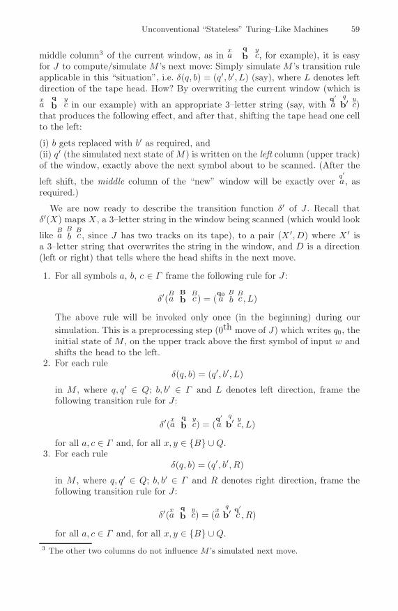
Unconventional “Stateless” Turing–Like Machines 59
middle column3 of the current window, as inxa
q
byc, for example), it is easy
for J to compute/simulate M ’s next move: Simply simulate M ’s transition ruleapplicable in this “situation”, i.e. δ(q, b) = (q′, b′, L) (say), where L denotes leftdirection of the tape head. How? By overwriting the current window (which isxa
q
byc in our example) with an appropriate 3–letter string (say, with
q′a
q
b′yc)
that produces the following effect, and after that, shifting the tape head one cellto the left:
(i) b gets replaced with b′ as required, and(ii) q′ (the simulated next state of M) is written on the left column (upper track)of the window, exactly above the next symbol about to be scanned. (After the
left shift, the middle column of the “new” window will be exactly overq′a, as
required.)
We are now ready to describe the transition function δ′ of J . Recall thatδ′(X) maps X , a 3–letter string in the window being scanned (which would look
likeBa
B
bBc , since J has two tracks on its tape), to a pair (X ′, D) where X ′ is
a 3–letter string that overwrites the string in the window, and D is a direction(left or right) that tells where the head shifts in the next move.
1. For all symbols a, b, c ∈ Γ frame the following rule for J :
δ′(Ba
B
bBc) = (
q0a
B
bBc , L)
The above rule will be invoked only once (in the beginning) during oursimulation. This is a preprocessing step (0th move of J) which writes q0, theinitial state of M , on the upper track above the first symbol of input w andshifts the head to the left.
2. For each ruleδ(q, b) = (q′, b′, L)
in M , where q, q′ ∈ Q; b, b′ ∈ Γ and L denotes left direction, frame thefollowing transition rule for J :
δ′(xa
q
byc) = (
q′a
q
b′yc, L)
for all a, c ∈ Γ and, for all x, y ∈ {B} ∪Q.3. For each rule
δ(q, b) = (q′, b′, R)
in M , where q, q′ ∈ Q; b, b′ ∈ Γ and R denotes right direction, frame thefollowing transition rule for J :
δ′(xa
q
byc) = (
xa
q
b′q′c , R)
for all a, c ∈ Γ and, for all x, y ∈ {B} ∪Q.3 The other two columns do not influence M ’s simulated next move.

60 J.J. Arulanandham
What remains now is to prove that the above construction is, indeed, correct.We will prove that the machines M and J will have the same configuration aftereach of them makes n moves, for any n ≥ 0. (This would automatically implythat both of them produce the same output for the same input.) Of course, Mmay not go on forever and would eventually halt if, at some point, no “nextmove” is defined; J would follow suit, since J too would not have a (corre-sponding) rule that dictates its next move. (Note that we do not count theinitial move of J as the “first move”, but as the “zeroth move”—a preprocess-ing step.) The proof is an easy induction on the number of moves of J and M .For the purposes of our proof, the configuration of a JTM will be describedsimply with the string X1X2 . . . Xi−1qXiXi+1 . . .Xn, where X1X2 . . . Xn is theportion of the tape (lower track only) between the leftmost and rightmost non-
blanks andq
Xi is the symbol in the middle column of the scanning window(the entire portions of the upper track, on the left and right of q, are omit-ted). Consider the basis case, i.e. when n = 0 (M is yet to make a move,and J has just executed the zeroth move). M ’s initial configuration will beq0X1X2 . . . Xn, where X1X2 . . . Xn = w, the input string, and q0, the initialstate of M . J would have had X1BX2 . . .Xn as its initial configuration (thatis how we set it up), but, after its zeroth move, it will become q0X1X2 . . . Xn
(according to transition rule 1), as required. Now, let us suppose that the con-figuration of both M and J is X1X2 . . .Xi−1qXiXi+1 . . . Xn after k moves.Then, after the (k + 1)th move, the configuration of both M and J will beeither:
(i) X1X2 . . . q′Xi−1Y Xi+1 . . . Xn, if the transition rule forM is δ(q,Xi)=(q′, Y, L)
(J would have applied transition rule 2), or(ii) X1X2 . . . Xi−1Y q
′Xi+1 . . . Xn, if the transition rule for M is δ(q,Xi) =(q′, Y, R)(J would have applied transition rule 3), as required. ��
4 Conclusion
It is traditionally known that Turing machines with only one state are not aspowerful as their counterparts with more number of states. We have shown thatthis is no longer the case if we modify the TM a little: by adding an extra feature,namely, reading/writing a 3–letter string (as opposed to reading/writing a singlesymbol). While this result may turn out to be a product of mere theoreticalcuriosity, we believe that JTMs could serve as normal forms that might makeproofs in computation theory simpler.
Acknowledgement
I thank my former colleague and friend, Mr. V. Ganesh Babu, for kindly readinga draft of my paper and for his remarks.

Unconventional “Stateless” Turing–Like Machines 61
References
1. Hopcroft, J.E., Motwani, R., Ullman, J.D.: Introduction to Automata Theory, Lan-guages, and Computation. Pearson Education, London (2006)
2. Turing, A.M.: On computable numbers with an application to the Entschei-dungsproblem. Proc. London Math. Society 2(42), 230–265 (1936)

Polarizationless P Systems
with Active MembranesWorking in the Minimally Parallel Mode
Rudolf Freund1, Gheorghe Paun2, and Mario J. Perez-Jimenez3
1 Institute of Computer LanguagesVienna University of Technology, Favoritenstr. 9, Wien, Austria
[email protected] Institute of Mathematics of the Romanian Academy
PO Box 1-764, 014700 Bucuresti, Romania, andDepartment of Computer Science and Artificial Intelligence
University of Sevilla, Avda. Reina Mercedes s/n, 41012 Sevilla, [email protected], [email protected]
3 Department of Computer Science and Artificial IntelligenceUniversity of Sevilla, Avda. Reina Mercedes s/n, 41012 Sevilla, Spain
Abstract. We investigate the computing power and the efficiency of Psystems with active membranes without polarizations, working in theminimally parallel mode. Such systems are shown to be computationallycomplete even when using only rules handling single objects in the mem-branes and avoiding the division of non-elementary membranes. More-over, we elaborate an algorithm for solving NP-complete problems, yetin this case we need evolution rules generating at least two objects aswell as rules for non-elementary membrane division.
1 Introduction
P systems with active membranes basically use five types of rules: (a) evolutionrules, by which a single object evolves to a multiset of objects, (b) send-in, and (c)send-out rules, by which an object is introduced in or expelled from a membrane,maybe modified during this operation into another object, (d) dissolution rules,by which a membrane is dissolved, under the influence of an object, which maybe modified into another object by this operation, and (e) membrane divisionrules; this last type of rules can be used both for elementary and non-elementarymembranes, or only for elementary membranes. As introduced in [9], all thesetypes of rules also use polarizations for membranes, “electrical charges” +,−, 0,controlling the application of the rules.
Systems with rules of types (a), (b), (c) were shown to be equivalent in com-putational power with Turing machines [10], even when using only two polariza-tions [4], while P systems using all types of rules were shown to be universal evenwithout using polarizations [1]. Another important class of results concerns the
S.G. Akl et al.(Eds.): UC 2007, LNCS 4618, pp. 62–76, 2007.c© Springer-Verlag Berlin Heidelberg 2007

Polarizationless P Systems with Active Membranes 63
possibility of using P systems with active membranes to provide polynomial so-lutions to computationally hard problems. Several papers have shown that bothdecision and numerical NP-complete problems can be solved in a polynomialtime (often, even linear time) by means of P systems with three polarizations[10], then the number of polarizations was decreased to two [3]. The systemsconstructed for these solutions use only division of elementary membranes. Atthe price of using division also for non-elementary membranes, the polarizationscan be removed completely [2].
All papers mentioned above apply the rules in the maximally parallel mode:in each computation step, the chosen multiset of rules cannot be extended any-more, i.e., no further rule could be added to this chosen multiset of rules insuch a way that the resulting extended multiset still could be applied. Recently,another strategy of applying rules in parallel was introduced, the so-called min-imal parallelism [5]: in each computation step, the chosen multiset of rules tobe applied in parallel cannot be extended by any rule out of a set of rules fromwhich no rule has been chosen so far for this multiset of rules in such a waythat the resulting extended multiset still could be applied (this is not the onlyway to interpret the idea of minimal parallelism, e.g., see [6] for other possi-bilities, yet the results elaborated in this paper hold true for all the variantsof minimal parallelism defined there). This introduces an additional degree ofnon-determinism in the system evolution, but still computational completenessand polynomial solutions to SAT were obtained in the new framework by usingP systems with active membranes, with three polarizations and division of onlyelementary membranes.
In this paper we continue the study of P systems working in the minimallyparallel way, and we prove that the polarizations can be avoided, at the price ofusing all five types of rules for computational completeness and even the divisionof non-elementary membranes for computational efficiency. On the other hand,in the proof for establishing computational completeness, in all types of rules wecan restrict their form to handling only single objects in the membranes (we callthis the one-normal form for P systems with active membranes).
2 Prerequisites
We suppose that the reader is familiar with the basic elements of Turing com-putability [7], and of membrane computing [10]. We here, in a rather informalway, introduce only the necessary notions and notation.
For an alphabet A, by A∗ we denote the set of all strings of symbols fromA including the empty string λ. A multiset over an alphabet A is a mappingfrom A to the set of natural numbers; we represent a multiset by a string fromA∗, where the number of occurrences of a symbol a ∈ A in a string w representsthe multiplicity of a in the multiset represented by w. The family of Turing-computable sets of natural numbers is denoted by NRE.
In our proofs showing computational completeness we use the characterizationof NRE by means of register machines. A register machine is a construct M =
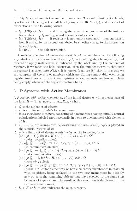
64 R. Freund, G. Paun, and M.J. Perez-Jimenez
(n,B, l0, lh, I), where n is the number of registers, B is a set of instruction labels,l0 is the start label, lh is the halt label (assigned to HALT only), and I is a set ofinstructions of the following forms:
– li : (ADD(r), lj , lk) add 1 to register r, and then go to one of the instruc-tions labeled by lj and lk, non-deterministically chosen;
– li : (SUB(r), lj , lk) if register r is non-empty (non-zero), then subtract 1from it and go to the instruction labeled by lj , otherwise go to the instructionlabeled by lk;
– lh : HALT the halt instruction.
A register machine M generates a set N(M) of numbers in the followingway: start with the instruction labeled by l0, with all registers being empty, andproceed to apply instructions as indicated by the labels and by the contents ofregisters. If we reach the halt instruction, then the number stored at that timein register 1 is taken into N(M). It is known (e.g., see [8]) that in this way wecan compute all the sets of numbers which are Turing-computable, even usingregister machines with only three registers as well as registers two and threebeing empty whenever the register machine halts.
3 P Systems with Active Membranes
A P system with active membranes, of the initial degree n ≥ 1, is a construct ofthe form Π = (O,H, μ,w1, . . . , wn, R, ho) where
1. O is the alphabet of objects ;2. H is a finite set of labels for membranes;3. μ is a membrane structure, consisting of nmembranes having initially neutral
polarizations, labeled (not necessarily in a one-to-one manner) with elementsof H ;
4. w1, . . . , wn are strings over O, describing the multisets of objects placed inthe n initial regions of μ;
5. R is a finite set of developmental rules, of the following forms:(a) [ha→ v]eh, for h ∈ H, e ∈ {+,−, 0}, a ∈ O, v ∈ O∗
(object evolution rules);(b) a[h ]e1
h → [hb]e2h , for h ∈ H, e1, e2 ∈ {+,−, 0}, a, b ∈ O
(in communication rules);(c) [ha ]e1
h → b[h ]e2h , for h ∈ H, e1, e2 ∈ {+,−, 0}, a, b ∈ O
(out communication rules);(d) [ha ]eh → b, for h ∈ H, e ∈ {+,−, 0}, a, b ∈ O
(dissolving rules);(e) [
ha ]e1
h→ [
hb ]e2
h[hc ]e3
h, for h ∈ H, e1, e2, e3 ∈ {+,−, 0}, a, b, c ∈ O
(division rules for elementary or non-elementary membranes in reactionwith an object, being replaced in the two new membranes by possiblynew objects; the remaining objects may have evolved in the same stepby rules of type (a) and the result of this evolution is duplicated in thetwo new membranes);
6. ho ∈ H or ho = env indicates the output region.

Polarizationless P Systems with Active Membranes 65
In all types of rules considered above, the labels of membranes are neverchanged. All the rules of any type involving a membrane h constitute the setRh, and for each occurrence of a membrane labelled by h we consider differentcopies of this set Rh. In the maximally parallel mode, in each step (a globalclock is assumed) we apply multisets of rules in such a way that no furtherrule can be applied to the remaining objects or membranes. In each step, eachobject and each membrane can be involved in only one rule. In the minimallyparallel mode, in each step, we choose a multiset of rules taken from the setsassigned to each membrane in the current configuration in such a way that af-ter having assigned objects to all the rules in this multiset, no rule from anyof the sets from which no rule has been taken so far, could be used in addi-tion. In every mode, each membrane and each object can be involved in onlyone rule, and the choice of rules to be used and of objects and membranes toevolve is done in a non-deterministic way. For rules of type (a) the membraneis not considered to be involved: when applying [ha → v]h, the object a can-not be used by other rules, but the membrane h can be used by any numberof rules of type (a) as well as by one rule of types (b) – (e). In each step,the use of rules is done in the bottom-up manner (first the inner objects andmembranes evolve, and the result is duplicated if any surrounding membrane isdivided).
A halting computation provides a result given by the number of objectspresent in region ho at the end of the computation; this is a region of the systemif ho ∈ H (and in this case, for a computation to be successful, exactly onemembrane with label ho should be present in the halting configuration), or it isthe environment if ho = env.
A system Π is said to be in the one-normal form if the membranes have nopolarization (it is the same as saying that always all membranes have the samepolarization, say 0, which therefore is irrelevant and thus omitted) and the rulesare of the forms [ha → b]h, a[h ]h → [hb]h, [ha ]h → b[h ]h, [ha ]h → b, and[ha ]h → [hb ]h[hc ]h, for a, b, c ∈ O, such that a �= b, a �= c, b �= c.
The set of numbers generated in the minimally parallel way by a system Π isdenoted by Nmin(Π). The family of sets Nmin(Π), generated by systems withrules of the non-restricted form, having initially at most n1 membranes and usingconfigurations with at most n2 membranes during any computation is denotedby NminOPn1,n2((a), (b), (c), (d), (e)); when a type of rules is not used, it is notmentioned in the notation. If any of the parameters n1, n2 is not bounded, thenit is replaced by ∗. If the systems do not use polarizations for membranes, thenwe write (a0), (b0), (c0), (d0), (e0) instead of (a), (b), (c), (d), (e). When the sys-tem Π is in the one-normal form, then we write NminOPn1,n2((a1), (b1), (c1),(d1), (e1)).
When considering families of numbers generated by P systems with activemembranes working in the maximally parallel mode, the subscript min is re-placed by max in the previous notations. For precise definitions, we refer to [10]and to the papers mentioned below.

66 R. Freund, G. Paun, and M.J. Perez-Jimenez
4 Computational Completeness
The following results are well known:
Theorem 1. (i) NmaxOP3,3((a), (b), (c)) = NRE, [10].(ii) NmaxOP∗,∗((a0), (b0), (c0), (d0), (e0)) = NRE, [1].(iii) NminOP3,3((a), (b), (c)) = NRE, [5].
In turn, the following inclusions follow directly from the definitions:
Lemma 1. NmodeOPn1,n2((a1), (b1), (c1), (d1), (e1)) ⊆NmodeOPn1,n2((a0), (b0), (c0), (d0), (e0)) ⊆NmodeOPn1,n2((a), (b), (c), (d), (e)),
for all n1, n2 ≥ 1, mode ∈ {max,min}.We now improve the equalities from Theorem 1 in certain respects, starting withproving the computational completeness of P systems with active membranes inthe one-normal form when working in the maximally parallel mode, and thenwe extend this result to the minimal parallelism.
Theorem 2. For all n1 ≥ 5,
NmaxOPn1,∗((a1), (b1), (c1), (d1), (e1)) = NRE.
Proof. We only prove the inclusion
NRE ⊆ NmaxOP5,∗((a1), (b1), (c1), (d1), (e1)).
Let us consider a register machine M = (3, B, l0, lh, I) generating an arbitraryset N(M) ∈ NRE. We construct the P system of initial degree 5
Π = (O,H, μ,ws, wh, w1, w2, w3, R, env),O = {di | 0 ≤ i ≤ 5} ∪ {g,#,#′, p, p′, p′′, c, c′, c′′} ∪B ∪ {l′ | l ∈ B}
∪ {liu | li is the label of an ADD instruction in I, 1 ≤ u ≤ 4}∪ {liu0 | li is the label of a SUB instruction in I, 1 ≤ u ≤ 4}∪ {liu+ | li is the label of a SUB instruction in I, 1 ≤ u ≤ 6},
H = {s, h, 1, 2, 3},μ = [s[1 ]1 [2 ]2 [3 ]3[h ]h]s,
ws = l0d0, wα = λ, for all α ∈ H − {s},with the rules from R constructed as described below.
The value stored in a register r = 1, 2, 3 of M , in Π is represented by thenumber of copies of membranes with label r plus one (if the value of the registerr is k, then we have k + 1 membranes with label r). The membrane with labelh is auxiliary, it is used for controlling the correct simulation of instructions ofM by computations in Π . Each step of a computation in M , i.e., using an ADDor a SUB instruction, corresponds to six steps of a computation in Π . We start

Polarizationless P Systems with Active Membranes 67
with all membranes being empty, except for the skin region, which contains theinitial label l0 of M and the auxiliary object d0. If the computation in M halts,that is, the object lh appears in the skin region of Π , then we pass to producingone object c for each membrane with label 1 present in the system, except one;in this way, the number of copies of c sent to the environment represents thecorrect result of the computation in M .
We now list the rules used in each of the six steps of simulating instructionsADD and SUB, and finally we present the rules for producing the result of thecomputation; in each configuration, only the membranes and the objects relevantfor the simulation of the respective instruction are specified. In particular, weignore the “garbage” object g, because once introduced it remains idle for thewhole computation.
The simulation of an instruction li : (ADD(r), lj , lk) uses the rules fromTable 1. The label object li enters into the correct membrane r (even if theregister r is empty, there is at least one membrane with label r) and in thenext step divides it. The object li2 exits the newly produced membrane, but gremains inside; li2 will evolve three further steps, just to synchronize with theevolution of the auxiliary objects du, u ≥ 0, and the auxiliary membrane h, sothat in the sixth step we end up with the label lj or lk of the next instructionto be simulated present in the skin membrane, together with d0; note that thenumber of copies of membrane r was increased by one.
Table 1. The simulation of an ADD instruction
Step Main rules Auxiliary rules Configuration
– – – [slid0 [
r]r. . . [
h]h]s
1 li[r]r→ [
rl′i]r
[sd0 → d1]s
[sd1 [
rl′i] r
. . . [h
]h]s
2 [rl′i]r
→ [rli1]r
[rg]
r[sd1 → d2]s
[sd2 [
rli1]r
[rg]
r. . . [
h]h]s
3 [rli1] r
→ li2[r]r
d2[h]h→ [
hd3]h
[sli2 [
r]r[r
]r. . . [
hd3]h
]s
4 [sli2 → li3]s
[hd3]h
→ d4[h]h
[sli3d4[r
]r[r
]r. . . [
h]h]s
5 [sli3 → li4]s
[sd4 → d5]s
[sli4d5[r
]r[r
]r. . . [
h]h]s
6 [sli4 → lt]s
, [sd5 → d0]s
[sltd0[r
]r[r
]r. . . [
h]h]s
t ∈ {j, k}
The auxiliary objects du, u ≥ 0, and the auxiliary membrane h are also used inthe simulation of SUB instructions; in step 4, there also are other rules to be usedin membrane h, introducing the trap object #, but using such rules will make thecomputation never halt, hence, they will not produce an unwanted result.
The evolution of the auxiliary objects du, u ≥ 0, is graphically representedin Figure 1; membrane h is only used in step 3, to send an object inside, andin the next step, for sending an object out of it. On each arrow we indicate thestep, according to Table 1; the steps made by using rules of types (b) and (c)are pointed out by drawing the respective arrows crossing the membranes, thussuggesting the in/out actions.
The way the simulation of an ADD instruction works is depicted in Figure 2;the division operation from step 2 is indicated by a branching arrow.
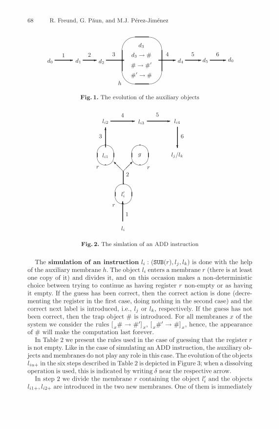
68 R. Freund, G. Paun, and M.J. Perez-Jimenez
�
�
�
�
d3
d3 → #
# → #′
#′ → #
d2d1d0 d4 d5 d0� � � � � �1 2 3 4 5 6
h
Fig. 1. The evolution of the auxiliary objects
li
�
�
�
�
�
�
�
�
�
r
l′i
li1 g
li2
�
��� ���
�
� li3� li4
lj/lk
�
r r
1
2
3
4 5
6
Fig. 2. The simlation of an ADD instruction
The simulation of an instruction li : (SUB(r), lj , lk) is done with the helpof the auxiliary membrane h. The object li enters a membrane r (there is at leastone copy of it) and divides it, and on this occasion makes a non-deterministicchoice between trying to continue as having register r non-empty or as havingit empty. If the guess has been correct, then the correct action is done (decre-menting the register in the first case, doing nothing in the second case) and thecorrect next label is introduced, i.e., lj or lk, respectively. If the guess has notbeen correct, then the trap object # is introduced. For all membranes x of thesystem we consider the rules [x# → #′]x, [x#′ → #]x, hence, the appearanceof # will make the computation last forever.
In Table 2 we present the rules used in the case of guessing that the register ris not empty. Like in the case of simulating an ADD instruction, the auxiliary ob-jects and membranes do not play any role in this case. The evolution of the objectsliu+ in the six steps described in Table 2 is depicted in Figure 3; when a dissolvingoperation is used, this is indicated by writing δ near the respective arrow.
In step 2 we divide the membrane r containing the object l′i and the objectsli1+, li2+ are introduced in the two new membranes. One of them is immediately
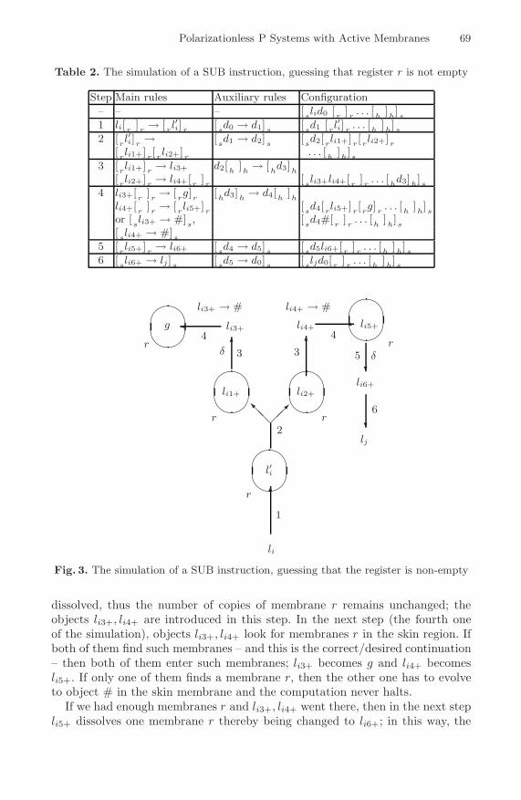
Polarizationless P Systems with Active Membranes 69
Table 2. The simulation of a SUB instruction, guessing that register r is not empty
Step Main rules Auxiliary rules Configuration
– – – [slid0 [
r]r. . . [
h]h]s
1 li[ r]r→ [
rl′i] r
[sd0 → d1]s
[sd1 [
rl′i] r
. . . [h
]h]s
2 [rl′i] r
→ [sd1 → d2]s
[sd2[ r
li1+]r[rli2+]
r
[rli1+]
r[rli2+]
r. . . [
h]h]s
3 [rli1+]
r→ li3+ d2[h
]h→ [
hd3]h
[rli2+]
r→ li4+[
r]r
[sli3+li4+[
r]r. . . [
hd3]h
]s
4 li3+[r
]r→ [
rg]
r[hd3]h
→ d4[h]h
li4+[r
]r→ [
rli5+]
r[sd4[ r
li5+]r[rg]
r. . . [
h]h]s
or [sli3+ → #]
s, [
sd4#[
r]r. . . [
h]h]s
[sli4+ → #]
s
5 [rli5+]
r→ li6+ [
sd4 → d5]s
[sd5li6+[
r]r. . . [
h]h]s
6 [sli6+ → lj ]s
[sd5 → d0]s
[sljd0[ r
]r. . . [
h]h]s
li
�
�
�
�
�
�
�
���
���
li3+
�
�
g
�
li4+ li5+
li6+
lj
�
�
�
�
�
�
r
r r
r r
1
2
3 3δ
4
li3+ → #
4
li4+ → #
5 δ
6
l′i
li1+ li2+
Fig. 3. The simulation of a SUB instruction, guessing that the register is non-empty
dissolved, thus the number of copies of membrane r remains unchanged; theobjects li3+, li4+ are introduced in this step. In the next step (the fourth oneof the simulation), objects li3+, li4+ look for membranes r in the skin region. Ifboth of them find such membranes – and this is the correct/desired continuation– then both of them enter such membranes; li3+ becomes g and li4+ becomesli5+. If only one of them finds a membrane r, then the other one has to evolveto object # in the skin membrane and the computation never halts.
If we had enough membranes r and li3+, li4+ went there, then in the next stepli5+ dissolves one membrane r thereby being changed to li6+; in this way, the

70 R. Freund, G. Paun, and M.J. Perez-Jimenez
Table 3. The simulation of a SUB instruction, guessing that register r is empty
Step Main rules Auxiliary rules Configuration
– – – [slid0 [
r]r. . . [
h]h]s
1 li[ r]r→ [
rl′i] r
[sd0 → d1]s
[sd1 [
rl′i] r
. . . [h
]h]s
2 [rl′i] r
→ [sd1 → d2]s
[sd2 [
rli10] r
[rli20]r
[rli10] r
[rli20]r
. . . [h
]h]s
3 [rli10] r
→ li30 d2[h]h→ [
hd3]h
[sli30li40 [
r]r
[rli20] r
→ li40[ r]r
. . . [hd3]h
]s
4 li30[r ]r → [rg]
r, [
hd3]h
→ d4[h]h
[sli40d4[ r
g]r. . . [
h]h]s
li40 waitsor li40[r
]r→ [
r#]
r[sd4[ r
#]r. . . [
h]h]s
or li40[h]h→ [
hl′k]
h[hd3 → #]
h[s[rg]
r. . . [
hl′k#]
h]s
5 li40[h]h→ [
hl′k]
h[sd4 → d5]s
[sd5[ r
]r. . . [
hl′k]
h]s
6 [hl′k]
h→ lk[
h]h
[sd5 → d0]s
[slkd0[ r
]r. . . [
h]h]s
number of membranes r has successfully been decremented. In the sixth step,li6+ finally becomes lj (simultaneously with regaining d0), and this completesthe simulation.
However, in step 2, instead of the rule [rl′i]r → [rli1+]r[rli2+]r we can use
the rule [rl′i]r → [rli10]r[rli20]r, with the intention to simulate the subtract
instruction in the case when the register r is empty – that is, only one membranewith label r is present in the system. The rules used in the six steps of thesimulation are given in Table 3.
The six steps of the simulation of a SUB instruction when guessing the corre-sponding register to be empty are shown in Figure 4, this time with the evolutionof the auxiliary objects being indicated, too. The arrows marked with # corre-spond to computations which are not desired.
In this case, the auxiliary objects du, u ≥ 0, and the auxiliary membrane hplay an essential role. Until step 3 we proceed exactly as above, but now weintroduce the objects li30 and li40. In step 4, li30 then can enter the availablemembrane r, there evolving to g. In this fourth step, there is a competitionbetween li40 and d3 for membrane h, but if li40 enters membrane h already inthis step, then the trap object # is produced here by the rule [hd3 → #]h.
If there is a second membrane r, i.e., if the guess has been incorrect, then– to avoid the scenario described before – the rule li40[r ]r → [r#]r has to beused simultaneously with li30[r ]r → [rg]r and [hd3]h → d4[h ]h in the fourthstep, yet then the computation never ends, too. If there is no second membraner, then, in step 4, li40 has to wait unchanged in the skin region if we applyli30[r ]r → [rg]r and [hd3]h → d4[h ]h in the desired way. Thus, the only waynot to introduce the object # is (i) not to have a second membrane r, (ii) to usethe rule [hd3]h → d4[h ]h, thus preventing the use of the rule li40[h ]h → [hl
′k]h
already in the fourth step, and (iii) not sending li40 to the unique membrane r.After having waited unchanged in the skin region during step 4, the object li40in the next step should enter membrane h (if entering the unique membrane r,

Polarizationless P Systems with Active Membranes 71
li
�
�
�
�
�
�
�
�
�
li30
li10
l′i
li20
li40
�
��� ���
� �
�
�
�
g
�
�
�
#�
�
�
�
��
���
l′k lk�
�
�
�
d3
�
d4 d5 d0d2d1d0� � � � � �1 2 3 4 5 6
h
d3 → #
#
4 5 h
r
4
#
33r
4
2
r r
δ
r
1
Fig. 4. The simulation of a SUB instruction, guessing that the register is empty
it becomes # there), and finally, lk is released from membrane h, at the sametime when d0 appears again.
If the computation in M halts by reaching lh, i.e., if the object lh is introducedin the skin region, we start to use the following rules:
lh[1 ]1 → [1l′h]1, [1l
′h]1 → p, p[1 ]1 → [1p
′]1,[1p′]1 → [1p
′′]1[1c′]1, [1p
′′]1 → p, [1c′]1 → c′′, [sc
′′]s → c[s ]s,
p[h ]h → [hp′]h, [hp
′]h → p.
The object lh dissolves one membrane with label 1 (thus, the remaining mem-branes with this label are now as many as the value of register 1 of M), and getstransformed into p. This object enters each membrane with label 1, divides itand then reproduces itself by passing through p′ and p′′, thereby also dissolvingone membrane with label 1, and also produces a copy of the object c′′, whichimmediately exits the system, thereby being changed into c.
At any time, the object p can also enter membrane h and then dissolve it.The computation can stop only after all membranes with label 1 having beendissolved (i.e., a corresponding number of copies of c has been sent out) and

72 R. Freund, G. Paun, and M.J. Perez-Jimenez
�
�
�
�
�
�
�
�
�
p �
�� �����
���
� c′′c′p′′
p′
δ
1
1 1
δc�out
�
�
�
l′hlh
� �
1
δ
�
�
�
��
������ �
���
����
h
p′
δ
Fig. 5. The end of computations
after the single membrane h having been dissolved, too, i.e., the evolution ofobjects du, u ≥ 0, is also stopped. The function of this final module is describedin Figure 5.
In sum, we conclude N(M) = Nmax(Π).
Theorem 3 gives the same result as Theorem 3 from [1], with the additionalconstraint to have evolution rules with exactly one object on the right-hand side(neither producing more objects, nor erasing objects, as it is the case in [1]).
The previous proof can easily be changed in order to obtain the computationalcompleteness of P systems in the one-normal form also in the case of minimalparallelism. Specifically, we can introduce additional membranes in order to avoidhaving two or more evolution rules to be applied in the same region or one ormore evolution rules and one rule of types (b) – (e) which involve the samemembrane:
– Applying any of the rules [sli3+ → #]s and [sli4+ → #]s, in step 4 of thesimulation of SUB for the guess of a non-empty register, means introducingthe trap object and is the same for the fate of the computation as applyingall possible rules of that kind.
– Steps 5 and 6 for the auxiliary rules are performed in the skin region, inparallel with steps of the main rules in the simulation of incrementing ordecrementing a register. This can be avoided by introducing one furtherauxiliary membrane, h′, in the skin region, and replacing the rules [sd4 →d5]s, [sd5 → d0]s (both of them from Rs) by the rules d4[h′ ]h′ → [h′d5]h′and [h′d5]h′ → d0[h′ ]h′ . These rules are associated with membrane h′,hence, they should be used in parallel with the rules from the skin region.
– A further case when the maximal parallelism is important in the previousconstruction is in step 4 of simulating a SUB instruction for the guess that

Polarizationless P Systems with Active Membranes 73
the register is empty: if rule li40[h]h→ [
hl′k]
his used in step 4, then also
the rule [hd3 → #]h must be used. In the minimally parallel mode, this canbe ensured if we replace this latter rule by d3[h′′ ]h′′ → [h′′#]h′′ , where h′′ isone further membrane, provided in the initial configuration inside membraneh. In this way, the rule d3[h′′ ]h′′ → [h′′#]h′′ involves the new membraneh′′, hence, it should be used in parallel with the rule li40[h ]h → [hl
′k]h. Of
course, we also need the rules [h′′# → #′]h′′ , [h′′#′ → #]h′′ , instead of thecorresponding rules from membrane h.
In this way, we obtain the following counterpart of Theorem 2 (note that weuse two further membranes, h′ and h′′):
Theorem 3. For all n1 ≥ 7,
NminOPn1,∗((as1), (bs1), (cs1), (ds1), (es1)) = NRE.
The previous systems can easily be modified in order to work in the acceptingmode: we introduce the number to be analyzed in the form of the multiplicityof membranes with label 1 initially present in the skin membrane (for numbern we start with n + 1 membranes [1 ]1 in the system) and we work exactlyas above, with the final module now having only the task of dissolving theauxiliary membrane with label h, thus halting the computation. Consequently,all the previous results, for both minimally and maximally parallel use of rules,are valid also for accepting P systems in the one-normal form.
5 Solving SAT by Polarizationless P Systems
We now turn our attention to applying P systems for deciding NP-completeproblems and give an efficient semi–uniform solution to the satisfiability prob-lem by using P systems with polarizationless active membranes working in theminimally parallel mode.
Theorem 4. The satisfiability of any propositional formula in the conjunctivenormal form, using n variables and m clauses, can be decided in a linear timewith respect to n by a polarizationless P system with active membranes, con-structed in linear time with respect to n and m, and working in the minimallyparallel mode.
Proof. Let us consider a propositional formula ϕ = C1 ∧ . . . ∧ Cm such thateach clause Cj , 1 ≤ j ≤ m, is of the form Cj = yj,1 ∨ . . . ∨ yj,kj , kj ≥ 1, foryj,r ∈ {xi,¬xi | 1 ≤ i ≤ n}. For each i = 1, 2, . . . , n, let us consider the twosubstrings t(xi) and f(xi) of c1 . . . cm such that, with 1 ≤ j ≤ m,t(xi) exactly contains the cj such that yj,r = xi for some r, 1 ≤ r ≤ kj ,f(xi) exactly contains the cj such that yj,r = ¬xi for some r, 1 ≤ r ≤ kj .
Thus, t(xi) and f(xi) describe the sets of clauses which take the value true whenxi is true and when xi is false, respectively.

74 R. Freund, G. Paun, and M.J. Perez-Jimenez
We construct the P system Π(ϕ) with the following components (the outputmembrane is not necessary, because the result is obtained in the environment):
O = {ai, fi, ti | 1 ≤ i ≤ n} ∪ {cj , dj | 1 ≤ j ≤ m} ∪ {pi | 1 ≤ i ≤ 2n+ 7}∪ {qi | 1 ≤ i ≤ 2n+ 1} ∪ {ri | 1 ≤ i ≤ 2n+ 5} ∪ {b1, b2, y, yes, no},
H = {s, s′, p, q, r, 0, 1, 2, . . . ,m},μ = [s[s′ [p ]p[0[q ]q[r]r[1 ]1[2 ]2 . . . [m ]m]0]s′ ]s,wp = p1, wq = q1, wr = r1, w0 = a1,
ws = ws′ = λ, wj = λ, for all j = 1, 2, . . . ,m.
The set of evolution rules, R, consists of the following rules:
(1) [ pi → pi+1]p, for all 1 ≤ i ≤ 2n+ 6,[ qi → qi+1]q, for all 1 ≤ i ≤ 2n,[ ri → ri+1]r, for all 1 ≤ i ≤ 2n+ 4.These rules are used for evolving counters pi, qi, and ri in membranes withlabels p, q, and r, respectively.
(2) [ai]0 → [fi]0[ ti]0, for all 1 ≤ i ≤ n,[ fi → f(xi)ai+1]0 and [ ti → t(xi)ai+1]0, for all 1 ≤ i ≤ n− 1,[ fn → f(xn)]0, [ tn → t(xn)]0.The goal of these rules is to generate the truth assignments of the n variablesx1, . . . , xn, and to analyze the clauses satisfied by xi and ¬xi, respectively.
(3) cj [ ]j → [ cj ]j and [ cj ]j → dj , for all 1 ≤ j ≤ m.In parallel with the division steps, if a clause Cj is satisfied by the previouslyexpanded variable, then the corresponding object cj enters membrane j inorder to dissolve it and to send objects dj to membrane 0.
(4) [ q2n+1 ]q → q2n+1[ ]q, [ q2n+1 → b1]0.The counter q produces an object b1 in each membrane 0.
(5) b1[ ]j → [ b1]j and [ b1] j → b2, for all 1 ≤ j ≤ m, [ b2 ]0 → b2.These rules allow to detect whether the truth assignment associated with amembrane 0 assigns the value false to the formula (in that case, the mem-brane 0 will be dissolved).
(6) [ p2n+7 ]p → p2n+7[ ]p, [p2n+7 ]s′ → no[ ]s′ , [no ]s → no[ ]s,[ r2n+5 ]r → r2n+5, [ r2n+5 ]0 → y[ ]0,[ y ]s′ → yes, [yes ]s → yes[ ]s.These rules produce the answer of the P system.
The membranes with labels p, q, and r, with the corresponding objects pi, qi,and ri, respectively, are used as counters, which evolve simultaneously with themain membrane 0, where the truth assignments of the n variables x1, . . . , xn aregenerated; the use of separate membranes for counters makes possible the correctsynchronization even for the case of the minimal parallelism. The evolution ofcounters is done by the rules of type (1). In parallel with these rules, membrane 0evolves by means of the rules of type (2). In odd steps (from step 1 to step 2n), wedivide the (non-elementary) membrane 0 (with fi, ti corresponding to the truthvalues false, true, respectively, for variable xi); in even steps we introduce the

Polarizationless P Systems with Active Membranes 75
clauses satisfied by xi,¬xi, respectively. After 2n steps, all 2n truth assignmentsfor the n variables have been generated and they are encoded in membraneslabeled by 0. If a clause Cj is satisfied by the previously expanded variable, thenthe corresponding object cj enters membrane j, by means of the first rule oftype (3), permitting its dissolution by means of the second rule of that type andsending objects dj to membrane 0. This is done also in step 2n+ 1, in parallelwith using the rules of type (1) and (4) for evolving membranes p, q, and r. Instep 2n+ 2, the counters pi and ri keep evolving and the second rule of type (4)produces an object b1 in each membrane 0.
After 2n+2 steps, the configuration C2n+2 of the system consists of 2n copiesof membrane 0, each of them containing the membrane q empty, the membraner with the object r2n+3, possible objects cj and dj , 1 ≤ j ≤ m, as well as copiesof those membranes with labels 1, 2, . . . ,m corresponding to clauses which werenot satisfied by the truth assignment generated in that copy of membrane 0. Themembranes associated with clauses satisfied by the truth assignments generatedhave been dissolved by the corresponding object cj . The membrane p containsthe object p2n+3, and membrane regions s′ and s are empty. Therefore, formulaϕ is satisfied if and only if there is a membrane 0 where all membranes 1, 2, . . . ,mhave been dissolved. The remaining rules allow for sending out an object yesto the environment in step 2n + 8, and, if the formula is not satisfiable, thenthe object no appears in step 2n+ 9. In both cases, this is the last step of thecomputation.
The system Π(ϕ) uses 9n+2m+18 objects, m+6 initial membranes, contain-ing in total 4 objects, and 9n+ 4m+ 20 rules. The number of objects generatedby any object evolution rule is bounded by m+1. Clearly, all computations stop(after at most 2n + 9 steps) and all give the same answer, yes or no, to thequestion whether formula ϕ is satisfiable, hence, the system is weakly confluent.These observations conclude the proof.
We can also design a deterministic P system Π(ϕ) working in minimally parallelmode which decides the satisfiability of ϕ; to this aim, it is enough to have mcopies of the object b1 in each membrane 0 of the configuration C2n+2, whichcan be obtained by replacing the rule [ q2n+1 → b1]0 by the rule [ q2n+1 → bm1 ]0.
The system used in the proof of Theorem 4 is not in the one-normal form,because some of the rules of type (b) in (2) are of the form [ha → u]h with ubeing an arbitrary multiset, hence, it remains an interesting open problem tofind a polynomial solution to SAT by a system in the one-normal form.
Acknowledgements. The work of Gh. Paun was partially supported by ProjectBioMAT 2-CEx06-11-97/19.09.06. The work of M.J. Perez-Jimenez was sup-ported by the project TIN2005-09345-C04-01 of the Ministerio de Educacion yCiencia of Spain, co–financed by FEDER funds, and of the project of ExcellenceTIC 581 of the Junta de Andalucıa. The authors also gratefully acknowledge theuseful comments of an unknown referee.

76 R. Freund, G. Paun, and M.J. Perez-Jimenez
References
1. Alhazov, A.: P systems without multiplicities of symbol-objects. Information Pro-cessing Letters 100, 124–129 (2006)
2. Alhazov, A., Perez-Jimenez, M.J.: Uniform Solution to QSAT Using Polarization-less Active Membranes. In: Vol. I of Proc. of the Fourth Brainstorming Week onMembrane Computing, Sevilla (Spain), pp. 29–40 (January 30 - February 3, 2006)
3. Alhazov, A., Freund, R.: Membrane Computing, International Workshop, WMC5,Milano, Italy, 2004, Selected Papers. In: Mauri, G., Paun, G., Perez-Jimenez,M.J., Rozenberg, G., Salomaa, A. (eds.) WMC 2004. LNCS, vol. 3365, pp. 81–94. Springer, Heidelberg (2005)
4. Alhazov, A., Freund, R., Paun, Gh.: Computational completeness of P systemswith active membranes and two polarizations. In: Margenstern, M. (ed.) MCU2004. LNCS, vol. 3354, pp. 82–92. Springer, Heidelberg (2005)
5. Ciobanu, G., Pan, L., Paun, Gh., Perez-Jimenez, M.J.: P systems with minimalparallelism. Theoretical Computer Science (to appear)
6. Freund, R., Verlan, S.: A formal framework for P systems. In: Proceedings WMC8, 2007 (to appear)
7. Hopcroft, J.E., Ullman, J.D.: Introduction to Automata Theory, Languages, andComputation. Addison-Wesley, Reading, MA (1979)
8. Minsky, M.: Computation – Finite and Infinite Machines. Prentice-Hall, EnglewoodCliffs, NJ (1967)
9. Paun, Gh.: P systems with active membranes: Attacking NP-complete problems.Journal of Automata, Languages and Combinatorics 6(1), 75–90 (2001)
10. Paun, Gh.: Membrane Computing. An Introduction. Springer, Heidelberg (2002)

On One Unconventional Framework for
Computation
Lev Goldfarb
Faculty of Computer ScienceUniversity of New Brunswick
Fredericton, [email protected]
http://www.cs.unb.ca/~goldfarb
Abstract. My main objective is to point out a fundamental weaknessin the conventional conception of computation and suggest a way out.This weakness is directly related to a gross underestimation of the roleof object representation in a computational model, hence confining suchmodels to an unrealistic (input) environment, which, in turn, lead to “un-realistic” computational models. This lack of appreciation of the role ofstructural object representation has been inherited from logic and partlyfrom mathematics, where, in the latter, the centuries-old tradition isto represent objects as unstructured “points”. I also discuss why theappropriate fundamental reorientation in the conception of computa-tional models will bring the resulting study of computation closer to the“natural” computational constrains. An example of the pertinent, class-oriented, representational formalism developed by our group over manyyears—Evolving Transformation System (ETS)—is briefly outlined here,and several general lines of research are suggested.
1 Introduction
Historically, computability theory has emerged within logic1, and so it is notsurprising that “logical” agenda continues to play an important part in its devel-opment2. This origin has determined to a considerable extent the basic “logicalorientation” of the field, i.e. the kinds of questions that one might be asking(computable vs. non-computable, etc.).3
1 E.g. Alan Turing proposed the Turing machine as a convenient mechanism for an-swering question of whether satisfiability in the predicate calculus was a solvableproblem or not.
2 E.g. Stephen Cook [1]: “When I submitted the abstract for this paper in December1970 my interest was in predicate calculus theorem proving procedures, and I hadnot yet thought of the idea of NP completeness.”
3 In connection with this orientation of the field, it is useful to recall ideas of JohnVon Neumann, one of the leading prewar logicians who was well aware of the originalTuring work and actually invited Turing to stay at the Institute for Advanced Studiesas his assistant (after Turing completed his Princeton dissertation): “We are very
S.G. Akl et al.(Eds.): UC 2007, LNCS 4618, pp. 77–90, 2007.c© Springer-Verlag Berlin Heidelberg 2007

78 L. Goldfarb
At the same time, already in his original paper, Turing had to face the issue ofrepresentation, both the “data” representation (on the tape), i.e. the input “sym-bol space”4, and the representation of the machine itself (machine instructionsand its states).
Following the original Turing’s considerations, related to “the process of [sym-bol] recognition”, it is not difficult to see that if these “symbols” would be endowedwith more general structure—as is the case with all real-world “symbols”—thestructure of the corresponding “generalized Turing machine”, or “intelligent ma-chine”, would have to be fundamentally modified in order to be able to deal withsuch structured symbols. So, first of all, we are faced with the ubiquitous issueof structural representation. Again, I would like to emphasize that, when dealingwith natural objects, the treatment of the issues related to the structural objectrepresentation must precede the computational considerations, since the formalstructure of the latter should depend on the formal structure of the former: thestructure of object operations will determine the structure of the correspondingbasic “machine” operations. Perhaps an analogy may help. If we recall the conceptof a mathematical structure (e.g. group, vector space, topological space, partiallyordered set), we should favor the idea that the structure of the machine operatingon the data that is viewed as an element of a particular (fixed) mathematical struc-ture should depend on the underlying operations postulated within this mathe-matical structure. In other words, representational considerations should precedecomputational ones.
However simple the above considerations may look, the looks are deceiving:it turns out that so far mathematics (and logic) has not adequately addressedthe issue of structural object representation, for good reasons. I suggest thatthese reasons are quite profound and have to do with the context within whichthe development of structural representation should take place. This context,of classes and induction, has never been adequately delineated neither within
far from possessing a theory of automata which deserves that name, that is, a purelymathematical-logical theory. There exists today a very elaborate system of formallogic and specifically, of logic as applied to mathematics. . . . About the inadequacies[of logic], however, this may be said: Everybody who has worked in formal logic willconfirm that it is one of the technically most refractory parts of mathematics. Thereason for this is that it deals with rigid, all-or-none concepts . . . . The theory ofautomata, of the digital, all-or-none type . . . is certainly a chapter in formal logic. Itwould, therefore, seem that it will have to share this unattractive property of formallogic.”[2].
4 “If we were to allow an infinity of symbols, then there would be symbols differingto an arbitrary small extent. . . . The new observed squares must be immediatelyrecognizable by the computer. . . . Now if these squares are marked only by singlesymbols there can be only a finite number of them, and we should not upset ourtheory by adjoining these marked squares to the observed squares. If, on the otherhand, . . . [each of them is] marked by a sequence of symbols [i.e. by a structuredsymbol], we cannot regard the process of recognition as a simple process. This is afundamental point and should be illustrated. [He then considers symbols formed bynumeric sequences.]”[3, my emphasis]

On One Unconventional Framework for Computation 79
philosophy—in spite of continuous attention it attracted over many centuries—nor within psychology, artificial intelligence, and information retrieval.
This paper is motivated by a recent development of the first such formalismfor structural representation, the Evolving Transformation System (ETS). Thereason I used adjective “first” has to do with the following considerations: despitethe common usage, strings and graphs cannot be considered as satisfactory formsof structural representation. Briefly, a string, for example, does not carry withinitself enough representational information to allow for the inductive recovery ofthe corresponding grammar, which, as it turns out, is a serious indication of theinadequacy of the underlying representational formalism. Not surprisingly, thedevelopment of such a radically different formalism as ETS is still in its initialstages, and hence, in this paper, it is prudent to focus on the overall directionsof its development rather than on any concrete formal results.
I should also mention that the above reorientation in the conception of a com-putational model is expected to bring it closer to a (structural) generalization ofthe conventional mathematical structures, in which the basic formal/underlyingstructure is postulated axiomatically.
2 On a Proper Approach to the Concept of StructuralObject Representation
Historically, mathematics has been the main, if not the only, “science of represen-tation”, so it is not surprising that the lack of appreciation of the role of objectrepresentation has been inherited from mathematics, where the centuries-old tra-dition has been to represent objects as unstructured “points”. In this sense, theunderestimation of the role of object representation in a computational modelis also not surprising. But while the mainstream mathematics—having been iso-lated from the problems arising in computer science—had no apparent impetusto proceed with the necessary radical developments, computer science has nosuch excuse. The concepts of data structure and abstract data type have been“screaming” for such fundamental developments. As was mentioned in Intro-duction, I believe the reasons for the lack of such developments within computerscience have to do with its historical roots in mathematical logic, whose devel-opment was not at all motivated5 by the representation of “physical” objects[4], [5].
First, I propose to proceed with the development of formalism for structuralrepresentation via generalization of the most basic entities on which the entireedifice of mathematics and natural sciences stands, i.e. via structural general-ization of the natural numbers: at this stage, I don’t think we have a morefundamental choice for our starting point. I do not have in mind here relatively“minor” (historical) generalizations such as complex numbers, quaternions, etc.,since such generalizations are still numeric-based. What I have in mind is more
5 I.e. considerably less so than is the case with mathematics, which always had toaddress the concerns of physics.

80 L. Goldfarb
far-reaching generalization, based on the generalization of the Peano construc-tive process in which a single simple successor operation is replaced by severalstructural ones. Thus I am suggesting entities that are structured in a mannershown in Figs. 1, 2.
Second, I suggest that the notion of structural representation can properlybe addressed only within the context of a class. The reasons have to do withthe following hypothesized ontology of objects. As we know, objects in naturedo not pop up out of nowhere but always take time to appear, and in each casethe way an object “appears” is similar to the way some other, “similar”, objectsappear, i.e. an object always appears as an element of some class of closelyrelated objects, be it an atom, a stone, a protein, or a stop sign. Moreover, anobject co-evolves also together with its class: there is an “invisible” permanent“bond” between an object and its class.
The crux of the proposed informational view of the universe can be expressedin the form of the first ontological postulate: in addition to the classes them-selves, for each class there exists, in some form, (its) class representation, whichmaintains the integrity of the class by guiding the generation of its new elements(and which therefore evolves together with the class). One should keep in mindthat this postulate can be seen as a continuation of a very remarkable line ofthought going back to Aristotle, Duns Scotus, and Francis Bacon, among others.
The second ontological postulate deals with the closely interconnected issuerelated to the nature of object representation: as is the case with a biological or-ganism, any object in nature exists along with its formative/generative history,which is recoverable from the above class representation. Hence the “similar-ity” of objects should now be understood as the “similarity” of their formativehistories. Since it is the object’s formative history that reveals its similarity ordissimilarity with other objects, this formative history must be captured in theobject’s “representation” (which is, in a sense, a generalization the fact that allbiological organisms store their developmental information). Actually, it is notdifficult to see that the two postulates are closely related, so that one “leads” tothe other.
Consistent with the above two postulates, one should approach the task ofdeveloping a formalism for structural representation as that of developing aclass-oriented representational formalism6, which would automatically ensurethat the formalism will be suitable for the purposes of inductive learning—sincethe object representation would carry much more information about its classrepresentation—and consequently for the purposes of AI in general.
It is useful to emphasize that the development of such an informational for-malism should not wait for the verification of the above hypotheses: for onething, no existing informational formalism insisted on any underlying hypoth-esis about the informational structure of the universe. I believe, however, thatin contrast to such practices, it is important to state up front an informationalhypothesis which would clarify and inform the development of the correspondinginformational formalism.
6 My papers [4], [5] are recommended as clarifying related issues.
On One Unconventional Framework for Computation 81
In what follows, I will proceed under the assumption that the above two pos-tulates are adopted, at least as far as the development of formalism for structuralrepresentation is concerned. Again, I would like to emphasize the importance ofsuch adoption: without the appropriate guiding considerations, the very notionof object representation becomes far too ambiguous, as can be seen from itsdevelopment so far. For example, strings and graphs are not appropriate modelsfor structural representation, since, as mentioned above, neither a string nor agraph carry within itself sufficient information for the inductive recovery of theclass from which it is supposed to come. This is, in part, a consequence of thesituation when none of the above two postulates have been adopted.
One more point regarding these postulates. If we recall Georg Cantor’s con-ception of the set as “the multitude that might be thought as oneness”, we cansee that the most natural way to conceive the multitude as one is to view theseobjects as elements of one class (specified via some generative mechanism, seesection 4). Thus, within the proposed “computational” setting, the underlyingformal structures come from those of classes.
3 The Price of Relying on Conventional DiscreteRepresentations
In this section, I want to address briefly the issue why the representation shouldbe of major concern when developing a computational model. First of all, Iassume (correctly or incorrectly) that the main objective of the present series ofconferences is to converge on the concept of computation that would be viable notjust within the “classical”, i.e. “logical”, setting but also in the natural sciencesin general.
The main problem with the conventional representations, such as strings,graphs, etc., is that they do not incorporate within themselves any particular(generative) structure that might be associated with their formation. However, aspostulated above (see the two postulates in section 2), this generative/formativestructure must be an integral part of an object’s identity, and when absent createsan unrealistic and ambiguous situation as to this identity. Such representationaldeficiency is obviously impossible to overcome. Indeed, for a string abbaca,there is simply no way to know the sequence of operations that was responsi-ble for the string formation and, potentially, there are exponentially many ofthem. As a consequence, from the very beginning we are critically handicappedin regards to our ability to discover the underlying generative structure, andno computational setting would be able to overcome this representational defi-ciency. To repeat, no amount of algorithmic maneuvering can recover the missingrepresentational information.
One might think that there is a simple way out of this situation: embed thenecessary formative information (via some tags) into the representation, end ofthe story. However, this is a typical representational kludge, as opposed to ascientific approach: we have not gotten wiser neither about structural objectrepresentation, nor about the concept of “formative history”.

82 L. Goldfarb
So now we come to a considerably less trivial question: What is a generalformalism for structural representation that would also explicate the notion ofstructural generativity as its integral part? Note that conventional computationalformalisms, for example Chomsky’s generative grammars, have not addressedthis issue simply because they had implicitly assumed that strings are legiti-mate forms of representation, so that this more fundamental representationalissue have not even appeared on the horizon (in spite of the fact that in thisparticular case Chomsky, from the very beginning, had emphasized the impor-tance of generativity). Of course, one can excuse these early developments sinceat the time of their emergence, 1930s to 1950s, the serious representational is-sues, could not have appeared on the horizon; but now, at the beginning of the21st century—when all kinds of applications, starting from general search en-gines (such as Google) and biological databases, all the way to various roboticapplications “beg” for structural representations—the story is quite different.
Thus, the price of relying on conventional discrete representations is thatthe more fundamental, underlying, representational formalism remained in thedark, which, in turn, prevented the development of a scientifically much moresatisfactory and definitive framework for computation, including the realizationof the full potential of many interesting ideas such as, to take a recent example,the membrane computing.
For a discussion of the inherent, or structural limitations of the two main con-ventional formalisms—vector space, or numeric, and logical—see [4], [5]. Inciden-tally, it is these inherent limitation of the numeric (representational) formalismthat, I believe, are responsible for the predominance of statistical over structuralconsiderations in machine learning, pattern recognition, data mining, informa-tion retrieval, bioinformatics, cheminformatics, and many other applied areas.The question is not whether the appropriate statistical considerations should playsome role in these areas, the obvious answer to which is “yes, of course”, but,as I emphasized above, whether, at present—when we lack any satisfactory for-malism for structural representation—we should be focusing on the developmentof new statistical techniques for the conventional formalisms that are inherentlyinadequate for dealing with classes (and hence, with the class-oriented needs ofthe above areas).
4 A Brief Sketch of the ETS Formalism
Unhappily or happily, the structure of this formalism has absolutely no analoguesto compare it with, despite the fact that its main entities, “structs”, may have asuperficial resemblance to some other known discrete objects such as, for example,graphs, which is useful to keep in mind. Also, in view of limited space, in what fol-lows I restrict myself to informal descriptions, while the formal definitions can befound in [6], Parts II and III. The most important point to keep in mind is that,in the formalism, all objects are viewed and represented as (temporal) structuralprocesses, in which the basic units are structured events, each responsible for trans-forming the flow of several “regular” processes (see Figs. 1, 2).

On One Unconventional Framework for Computation 83
4.1 Primitive Transformations
The first basic concept is that of a primitive transformation, or primitive event,or simply primitive, several of which are depicted in Fig. 1. In contrast to the ba-sic units in conventional formalisms, this concept “atomic” to the ETS formalismis relatively non-trivial, carrying both semantic and syntactic loads. It stands for afixed “micro-event” responsible for transforming one set of adjacent/interactingprocesses, called initial processes, into another set of processes, called terminalprocesses (in Fig. 2, both are shown as lines connecting primitives). In other words,the concept of primitive transformation encapsulates that of a “standard”/fixedinteraction7 of several processes, where each belongs to a particular class of pri-mal processes, or a primal class8. One can assume that the processes involvedare “periodic” and the event is responsible for their partial or complete modifi-cation into another set of periodic processes. The formal structure of the event issuch that it does not depend on the concrete initial (or concrete terminal) pro-cess, as long as each of the processes involved belongs to the same (fixed) primalclass of processes depicted in Fig. 1 as a small solid shape at the top (or at thebottom) of the event. As one can see, at this, basic, (or 0th), stage of representa-tion9, the structure of the initial and terminal processes is suppressed, as is theinternal structure of the transforming event itself, and what’s being captured bythe formal structure is the “external” structure of the event.
Fig. 1. Pictorial illustration of three primitives. The first subscript of a primitive refersto the class of primitives all sharing the same structure, e.g. π2b and π2d . The initialclasses are marked as various shapes on the top, while the terminal classes are shownas shapes on the bottom: each shape stands for a particular class of processes. Theonly concrete processes—i.e. elements of these classes—identified in the figure as theinitial processes of the primitive π2b with label b = 〈 c1
i , c2j , c3
k 〉 , where cst is the
tth process from primal class Cs, s = 1, 2, 3 .
Since all of nature is composed of various temporal processes, examples of theabove events are all around us: e.g. elementary particle collision, formation ofa two-cell blastula from a single cell (initial process is the original cell and theterminal processes are the resulting two cells), collision of two cars, the eventassociated with the transforming effect on the listener’s memory of the sentence
7 The internal structure of such event/interaction is undisclosed.8 The concept of class permeates all levels of consideration.9 In this paper, I discuss only a single-stage version of ETS. For multi-stage version see
[6], Part IV.

84 L. Goldfarb
“Alice and Bob had a baby” (initial processes are Alice and Bob and the termi-nal processes are Alice, Bob, and the baby), etc., where each mentioned eventtransforms the “flow” of the corresponding stable/regular processes involved.
4.2 Structs
The second basic concept is that of a struct formed by a (temporal) sequenceof the above primitive events, as shown in Fig. 2. It should be easy to see howthe temporal process of Peano construction of natural numbers (see Fig. 3) wasgeneralized to the construction of structs: the single “structureless” unit out ofwhich a number is built was replaced by multiple structural ones. An immediateand important consequence of the distinguishability (or multiplicity) of units inthe construction process is that we can now see which unit was attached andwhen. Hence, the resulting (object) representation for the first time embodiesboth temporal and structural information in the form of a formative, or gener-ative, object history recorded as a series of (structured) events. This was one ofthe basic driving motivations for the development of ETS, while the other mainmotivation was the development of a unified class-oriented representational for-malism that would satisfy the needs of a large variety of information-processingareas as well as natural sciences.
Fig. 2. Two illustrative examples of (short) structs
4.3 Struct Assembly
One of the basic operations on structs is struct assembly (as depicted in Fig. 4),which relies on the events shared by the structs involved. This operation allowsone to combine in one struct several separately observed, but typically overlap-ping, structs (e.g. those representing several facial features such as the eyes andthe nose). In particular, the overlap of several structs representing several actualprocesses captures a “non-interfering” interaction of these processes.
It is not difficult to see now the fundamental difference between a struct and,for example, a string: the main difference has to do with the temporal nature

On One Unconventional Framework for Computation 85
Fig. 3. The single primitive involved in the ETS representation of natural numbers,and three structs representing the numbers 1, 2, and 3
of ETS representation, which allows one to “compare” any objects based ontheir “formative history”. The latter information is simply not available in allconventional forms of representation.
Thus, to repeat, the ETS object representation captures the object’s forma-tive/generative history which, for the first time, brings considerable additionalinformation into the object representation. I should add that, from the appliedpoint of view, the adjective “formative” does not (and cannot) refer to the ob-ject’s actual formative history, since, in many cases, it is not accessible to us,but rather to a particularly chosen application mode of approaching/recordingit, i.e. to the mode of struct construction selected by the application developers.
4.4 Level 0 Classes
The third basic concept is that of a class. Even within the basic representationalstage—the only one I discuss here—each class10 is also viewed as possibly multi-leveled. A single-level class representation is specified by means of a single-level, or level 0, class generating system, which details the stepwise modeof construction of the class elements.11 Each (non-deterministic) step in sucha system is specified by a set of (level 0) constraints. Each constraint—also amajor concept, which not introduced here—is a formal specification of a family ofstructs sharing some structural “components” in the form of common substructs.During a step in the construction process, the struct that is being attached(at this step) to the part of the class element that has been assembled so farmust satisfy one of the constraints for this step. To be more accurate, in thedefinition, it is assumed that each such step can be preceded by a step executedby the “environment”, i.e. by some other class generating system “intervening” or“participating” in the construction process (see Fig. 5). Thus, quite appropriatelyand realistically, a change in the environment may result in a class change,
10 Here, I do not include the primal classes, which are assumed to be of undisclosedstructure.
11 Note that since we began with level 0, it cannot recurse to any lover level; level 1 isbuilt on top of level 0; level 2 is built on top of level 1; etc. Also note the differencebetween a level and a stage (see the next subsection): levels refer to those of classesand appear within a single representational stage.

86 L. Goldfarb
Fig. 4. Three structs and their assembly. Note that the second link connecting prim-itives π3k and π2g in the assembly comes from σ1 (but not from σ3 , despite thedelineation of σ3 with a bold line).
without an attendant change in the class generating system itself. Such a conceptof class admits the effects of the environment in a “natural” manner.
4.5 Level 1 Structs
Suppose that an agent has already learned several level 0 classes, which togetherform the current level 0 class setting. Then, when representing objects, the agenthas an access to a more refined form of object representation than a plain level0 struct: it can now see if this struct is in fact composed of several level 0 classelements (each belongs to one of the classes in level 0 class setting, see Fig. 6).This leads to the concept of the next level (level 1) struct, which provides extra

On One Unconventional Framework for Computation 87
Fig. 5. Pictorial representation of a generic two-step generative “unit” in the construc-tion of a class element: a step by the environment (bottom shaded primitives in thesecond struct, added to the first one) followed by a step made by the class generatingsystem (substruct βj in the third struct attached to the second struct)
Fig. 6. Simplified pictorial representation of a level 1 struct in the contracted form:dots stand for primitives and solid lines delineate level 0 class elements ci’s
representational information as compared to the underlying level 0 struct in theform of the appropriate partition of the previous level (level 0) struct.

88 L. Goldfarb
4.6 Higher Level Classes
In the (recursive) k-level version of the class representation, for k ≥ 2, eachstep is associated with a set of level (k − 1) constraints. However, during theconstruction process, level (k−1) struct that is being attached (at this step) tothe previously constructed part must now be composed only out of level (k−2)admissible class elements12 in a manner satisfying one of the constraints for thisstep. Figure 7 illustrates this construction process for level 1 class element.
For a level 2 class element this element is an output of a level 2 (or three-levels) class generating system at each step of its construction, the relevant partis assembled out of several level 1 class elements in accordance with one of theconstraints specified for this step.
Fig. 7. Illustration of a generic two-step generative unit in the construction of somelevel 1 class element. Dots stand for primitives, and solid lines delineate level 0 classelements, which now serve as simplest construction units. A step by the environment(bottom left gray addition in the second struct) is followed by a step made by a level1class generating system itself (struct delineated by the dotted line).
5 Some Initial Computational Questions Arising Withinthe ETS Formalism
For simplicity, I discuss only a basic single-stage computational “agenda” withinthe ETS formalism, which can be stated in the following form: Given an ab-stract delineation of a family of multi-level classes (or class generating systems)and given several 0-level (“training”) structs from a class belonging to the givenfamily, the goal is to “extract” the corresponding class generating system.
In other words, I suggest that within such (inductive) framework, the com-putational theory is aimed at developing the theory and techniques that wouldallow one, first, to preprocess (or partition, or “mark up”) the input structs in12 Each of those must come from a class belonging to a (previously learned or given)
set of level (k − 2) classes, comprising level (k − 2) class setting.

On One Unconventional Framework for Computation 89
a consistent manner, based on the structure of the given family of multi-levelclasses; and then one can proceed to the extraction of the underlying class gen-erating system.
So first of all, one would need to develop a corresponding structural theory,which could be thought of as a “structural” generalization of the Chomsky’s lan-guage hierarchy. As in the case of Chomsky hierarchy, such a theory would allowone to restrict the above problem to a particular (structural) family of classes.The development of such a hierarchy should probably proceed along the linessomewhat similar to those followed by Chomsky, with the following quite naturaladjustment: within the hierarchy, each family of classes should be introduced viathe appropriate restriction on the set of admissible constraints—which are theETS analogues of the production rules—involved in the specification of the class.However, it is also important to emphasize the differences between the ETS andthe conventional string (and graph hierarchies), and such differences concern notjust the presence of levels in ETS. When defining a conventional, for exampleChomsky, hierarchy, one is not treating a string as a form of object representationas understood above. This results, on the one hand, in a wider range of admis-sible production rules (not all are meaningful from the representational pointof view), and on the other hand, in a variety of qualitatively different machinesassociated with each family of languages (e.g. deterministic/nondeterministic).There are reasons to believe that, in the case of ETS formalism, in view of thetemporal form of representation, the situation is more palatable.
Next, based on such a structure theory, one would need to develop techniquesfor the above class related (structural) preprocessing, or partitioning, of thestructs in a given (training) set of structs. Even this task is highly non-trivial,since the tiling of each given struct must be accomplished relying on the admis-sible previous level class elements only (see Fig. 6). The final stage is related tothe construction of the corresponding class representation.
It is understood that, in the meantime, to proceed with various applications,one does not need to wait for the development of a full-fledged structural theory,since in each concrete application, the corresponding family of classes can readilybe specified.X
Thus, it should be clear that in contrast to the conventional computationalmodels—where, as was mentioned above, the defining agenda was logical—Ipropose that it is the (structural) inductive agenda that should now drive thedevelopment of the computational framework. This proposal is not really surpris-ing, given that the new framework is aimed at supporting a continuous dynamicinteraction between the “machine” and various natural environments, where, aswas hypothesized above, the temporal/structural nature of object representationis ubiquitous.
6 Conclusion
I hinted that it might be prudent for some researchers in computation to add totheir research interests a new area that we called Inductive Informatics, whichcan be thought of as a reincarnation of a four-hundred-year-old Francis Bacon’s

90 L. Goldfarb
project of putting all sciences on firm inductive footing, with the attendantrestructuring of the basic formal language and methodology. In hindsight, it ap-pears that the major obstacle has been the lack of a classification-oriented—orwhich appears to be the same thing “structural”—representational formalism.Our proposed version of such formalism is a far-reaching, structural, general-ization of the numeric representation, and in that sense it is much closer tomathematics than the logic, which was suggested by von Neumann [2] to be adesirable direction. Moreover, with the appearance of such a formalism, the con-cept of class representation, for the first time, becomes meaningful, and it alsobecomes quite clear that it is the intrinsic incapability of the conventional repre-sentational formalisms to support this fundamental concept that is responsiblefor our previous failure to realize Bacon’s vision.
In addition to the new theoretical horizons that are being opened up withinnew (event-based) representational formalisms, the other main reason why suchformalisms should be of interest to researchers in computation has to do withthe immediate practical benefits one can derive from their various applications inmachine learning, pattern recognition, data mining, information retrieval, bioin-formatics, cheminformatics, and many other applied areas. The validity of thelast statement should become apparent if one followed carefully the above pointregarding the new and rich aspect of object representation—i.e. the object’s for-mative history—that now becomes available within the ETS formalism.
Acknowledgment. I thank Oleg Golubitsky for a discussion of the paper andIan Scrimger for help with formatting.
References
1. Cook, S.A.: The complexity of theorem proving. In: Laplante, P. (ed.) Great Papersin Computer Science, vol. 2, West Publishing Co. St. Paul, Minneapolis (1996)
2. Neumann, von J.: The general and logical theory of automata. In: Pylyshyn, Z.W.(ed.) Perspectives in the Computer Revolution, pp. 99–100. Prentice-Hall, Engle-wood Cliffs, New Jersey (1970)
3. Turing, A.M.: On computable numbers, with an application to the Entschei-dungsproblem. In: Laplante, P. (ed.) Great Papers in Computer Science, pp. 303–304. West Publishing Co. St. Paul, Minneapolis (1996)
4. Goldfarb, L.: Representational formalisms: What they are and why we haven’t hadany. In: Goldfarb, L. (ed.) What Is a Structural Representation (in preparation)http://www.cs.unb.ca/∼goldfarb/ETSbook/ReprFormalisms.pdf
5. Goldfarb, L.: On the Concept of Class and Its Role in the Future of Machine Learn-ing. In: Goldfarb, L. (ed.) What Is a Structural Representation (in preparation)http://www.cs.unb.ca/∼goldfarb/ETSbook/Class.pdf
6. Goldfarb, L., Gay, D., Golubitsky, O., Korkin, D.: What is a structural represen-tation? A proposal for an event-based representational formalism. In: Goldfarb, L.(ed.) What Is a Structural Representation (in preparation)http://www.cs.unb.ca/∼goldfarb/ETSbook/ETS5.pdf

Computing Through Gene Assembly
Tseren-Onolt Ishdorj1,3 and Ion Petre1,2
1 Computational Biomodelling LaboratoryDepartment of Information Technologies
Abo Akademi University, Turku 20520 Finland{tishdorj,ipetre}@abo.fi
2 TUCS, Turku 20520 Finland3 Research Group on Natural Computing
Department of CS and AI, Sevilla UniversityAvda. Reina Mercedes s/n, 41012 Sevilla, Spain
Abstract. The intramolecular gene assembly model, [1], uses threemolecular recombination operations ld, dlad, and hi. A computing modelwith two contextual recombination operations del and trl , which arebased on ld and dlad, respectively, is considered in [6] and its computa-tional power is investigated. In the present paper, we expand the comput-ing model with a new molecular operation such as cpy - copy. Then weprove that the extended contextual intramolecular gene assembly modelis both computationally universal and efficient.
1 Introduction
There have been proposed two formal models to explain the gene assembly pro-cess in ciliates: intermolecular model, for instance in [8], and intramolecularmodel, for instance in [1]. They both are based on so called “pointers” - shortnucleotide sequences (about 20 bp) lying on the borders between coding andnon-coding blocks. Each next coding block starts with a pointer-sequence re-peating exactly the pointer-sequence in the end of the preceding codding blockfrom the assembled gene. It is supposed that the pointers guide the alignmentof coding blocks during the gene assembly process. The intramolecular modelproposes three operations: ld (loop with direct pointers), hi (hairpin loop withinverted pointers), dlad (double loop with alternating direct pointers).
The context sensitive variants of the intramolecular operations dlad and ldhave been considered in [6]. The accepting contextual intramolecular recom-bination (AIR) system using the operations translocation based on (dlad) anddeletion based on (ld) has been proved to be equivalent in power with Turingmachine.
In the present paper, we expand the set of contextual intramolecular oper-ations with a new operation: copy cpyp. Intramolecular copy operation is firstconsidered in [14]. The extended intramolecular recombination model with threetypes of contextual operations translocation, deletion, and copy computing alonga single string is as powerful as Turing machine, and efficient enough to solveNP-complete problems (in particular, SAT) in polynomial time.
S.G. Akl et al.(Eds.): UC 2007, LNCS 4618, pp. 91–105, 2007.c© Springer-Verlag Berlin Heidelberg 2007

92 T.-O. Ishdorj and I. Petre
No ciliate-based efficient algorithm for intractable problems has been pre-sented in the literature so far. This makes the efficiency result in this papernovel in the theory of ciliate computation.
A particularly interesting feature of the system is that the recombinationoperations are applied in a maximally parallel manner.
To solve an instance of SAT, we encode the problem into a string. Then duringthe recombination steps, the encoded problem (propositional formula) is du-plicated by copy operation along the string. Meanwhile, the truth-assignmentsattached to the propositional formula are constructed. In the end, all possibletruth-assignments are generated in a linear number of steps, and each truth-assignment is checked to see whether it satisfies the encoded formula.
The universality result of [6] uses a number of copies of a given substring alongthe working string in order to start a computation. By extension of the modelwith the copy operation, the necessary substrings will be generated during thecomputation instead of making the working string as full storage in advance asin [6]. This saves on the size and complexity of the encoding.
2 Preliminaries
We assume the reader to be familiar with the basic elements of formal languagesand Turing computability [13], DNA computing [12], and computational com-plexity [10]. We present here only some of the necessary notions and notation.
Using an approach developed in a series of works (see [9], [11], [2], and [7])we use contexts to restrict the application of molecular recombination opera-tions, [12], [1]. First, we give the formal definition of splicing rules. Consider analphabet Σ and two special symbols, #, $ /∈ Σ. A splicing rule (over Σ) is astring of the form r = u1#u2$u3#u4, where u1, u2, u3, u4 ∈ Σ∗. (For a maximalgenerality, we place no restriction on the strings u1, u2, u3, u4. The cases whenu1u2 = λ or u3u4 = λ could be ruled out as unrealistic.)
For a splicing rule r = u1#u2$u3#u4 and strings x, y, z ∈ Σ∗ we write(x, y) �r z if and only if x = x1u1u2x2, y = y1u3u4y2, z = x1u1u4y2, forsome x1, x2, y1, y2 ∈ Σ∗. We say that we splice x, y at the sites u1u2, u3u4,respectively, and the result is z. This is the basic operation of DNA moleculerecombination.
A splicing scheme [5] is a pair R = (Σ,∼), where Σ is the alphabet and∼, the pairing relation of the scheme, ∼⊆ (Σ+)3 × (Σ+)3. Assume we havetwo strings x, y and a binary relation between two triples of nonempty words(α, p, β) ∼ (α′, p, β′), such that x = x′αpβx′′ and y = y′α′pβ′y′′; then, thestrings obtained by the recombination in the context from above are z1 =x′αpβ′y′′ and z2 = y′α′pβx′′. When having a pair (α, p, β) ∼ (α′, p, β′) andtwo strings x and y as above, x = x′αpβx′′ and y = y′α′pβ′y′′, we considerjust the string z1 = x′αpβ′y′′ as the result of the recombination (we call it one-output-recombination), because the string z2 = y′α′pβx′′, we consider as theresult of the one-output-recombination with the respect to the symmetric pair(α′, p, β′) ∼ (α, p, β).

Computing Through Gene Assembly 93
A rewriting system M = (S,Σ ∪ {#}, P ) is called a Turing machine (we usealso abbreviation TM), [13], where: (i) S and Σ∪{#}, where # /∈ Σ and Σ �= ∅,are two disjoint sets referred to as the state and the tape alphabets; we fix asymbol from Σ, denote it as and call it “blank symbol”; (ii) Elements s0 andsf of S are the initial and the final states respectively; (iii) The productions(rewriting rules) of P are of the forms
(1) sia −→ sjb; (2) siac −→ asjc; (3) sia# −→ asj #; (4) csia −→ sjca;(5) #sia −→ #sj a; (6) sfa −→ sf ; (7) asf −→ sf , where si and sj arestates in S, si �= sf , and a, b, c are in Σ.
The TM M changes from one configuration to another one according to its setof rules P . We say that the Turing machine M halts with a word w if there existsa computation such that, when started with the read/write head positioned atthe beginning of w, the TM eventually reaches the final state, i.e., if #s0w#derives #sf# by successive applications of the rewriting rules (1)–(7) from P .The language L(M) accepted by the TM M is the set of words on which Mhalts. If TM is deterministic, then there is the only computation possible foreach word. The family of languages accepted by Turing machines is equivalentto the family of languages accepted by deterministic Turing machines.
The satisfiability problem, SAT, is a well known NP-complete problem. It askswhether or not for a given propositional formula in the conjunctive normal formthere is a truth-assignment of variables such that the formula assumes the valuetrue. The details of SAT are considered in Section 4.
3 The Contextual Intramolecular Operations
The contextual intramolecular translocation and deletion operations are the gen-eralizations of dlad and ld operations, respectively, as defined in [6]. We considera splicing scheme R = (Σ,∼). Denote core(R) = {p | (α, p, β) ∼ (γ, p, δ) ∈ R forsome α, β, γ, δ ∈ Σ+}.Definition 1. The contextual intramolecular translocation operation with re-spect to R is defined as trlp,q(xpuqypvqz) = xpvqypuqz, where there are suchrelations (α, p, β) ∼ (α′, p, β′) and (γ, q, δ) ∼ (γ′, q, δ′) in R, that x = x′α,uqy = βu′ = u′′α′, vqz = β′v′, xpu = x′′γ, ypv = δy′ = y′′γ′ and z = δ′z′.
We say that operation trlp,q is applicable, if the contexts of the two occurrencesof p as well as the contexts of the two occurrences of q are in the relation ∼.Substrings p and q we call pointers. In the result of application of trlp,q stringsu and v, each flanked by pointers p and q, are swapped. If from the non-emptyword u we get by trlp,q operation word v, we write u =⇒trlp,q
v and say that vis obtained from u by trlp,q operation. The translocation is depicted in Fig. 1.
Definition 2. The contextual intramolecular deletion operation with respect toR is defined as delp(xpupy) = xpy, where there is a relation (α, p, β) ∼ (α′, p, β′)in R that x = x′α, u = βu′ = u′′α′, and y = β′y′.

94 T.-O. Ishdorj and I. Petre
p p q� q� � � � ��� �� ��¤$ ...
p p q� q� � � � �� � �� ��¤ $...
trlp,q(x)=y
x
y
�trlp
,q
( p ) ( ’p ’) ( q ) ( ’q ’)� � � � � � � �and~ ~
... ...
... ...
Fig. 1. Translocation operation
In the result of applying delp, the string u flanked by two occurrences of p isremoved, provided that the contexts of those occurrences of p are in the relation∼. If from a non-empty word u we obtain a word v by delp, we write u =⇒delp
vand say that the word v is obtained from u by delp operation. See Fig. 2 A.
(x)=ycpyq
x
y
�cpy
q
where ( q$) ($q ’)� �~
q q� $ ��$
�p p� � � ���$p p� � � ���$
�
x
y
�delp
delp(x)=y ( p ) ( ’p ’)where � � � �~
A. B.
� �p
� q $ q �
Fig. 2. A. Deletion and B. Copy operations
We introduce here an additional operation the contextual intramolecular copy.
Definition 3. The contextual intramolecular copy operation with respect to R isdefined as cpyq(xquqy) = xquuqy, where there is a relation (α, q, β) ∼ (α′, q, β′)in R that x = x′α, u = β = α′, y = β′y′.
As a result of applying cpy q, the substring u flanked by two occurrences of qis duplicated. The substring u supposed to be duplicated itself must be alsothe following substring of the first pointer q and the preceding substring of thesecond occurrence of q. If from the non-empty word u we obtain a word v bycpyq, we write u =⇒cpy
qv and say that the word v is obtained from u by cpyq
operation. The copy operation is depicted in Fig. 2 B.We use the next notations:
trl = {trlp,q | p, q ∈ core(R)},del = {delp | p ∈ core(R)},cpy = {cpyp | p ∈ core(R)}.
Then we define the set of all contextual intramolecular operations as follows:R = trl ∪ del ∪ cpy .
Definition 4. Let a triplet Rop = (Σ,∼, op) be a splicing scheme that an oper-ation op ∈ R performs only in the contexts defined by the set of splicing relationsin Rop. We say that Rop is an operation class of the splicing scheme ∼ for theoperation op ∈ R.

Computing Through Gene Assembly 95
We consider the parallelism for the intramolecular recombination model. In-tuitively, a number of operations can be applied in parallel to a string if theapplicability of each operation is independent of the applicability of the otheroperations. The parallelism in intramolecular gene assembly was initially studiedin a different setting in [4]. We recall the definition of parallelism following [4]with a small modification adapted to our model.
Definition 5. Let S ⊆ R be a set of k rules and let u be a string. We say thatthe rules in S can be applied in parallel to u if for any ordering ϕ1, ϕ2, . . . , ϕk
of S, the composition ϕk ◦ ϕk−1 ◦ · · · ◦ ϕ1, is applicable to u.
In our proof below we use a different notion of parallelism. We introduce it hereis the form of the maximally parallel application of a rule to a string. First, wedefine the working places of a operation ϕ ∈ R on a given string where ϕ isapplicable.
Definition 6. Let w be a string. The working places of a operation ϕ ∈ R forw is a set of substrings of w written as Wp(ϕ(w)) and defined by
Wp(trlp,q(w)) = {(w1, w2) ∈ Sub(w) | trlp,q(xw1yw2z) = xw2yw1z}.Wp(delp(w)) = {w1 ∈ Sub(w) | delp(xpw1py) = xpy}.Wp(cpyp(w)) = {w1 ∈ Sub(w) | cpyp(xw1y) = xw1w1y}.
Definition 7. Let w be a string. The smallest working places of an operationϕ ∈ R for w is a subset of Wp(ϕ)(w) written as Wps(ϕ(w)) and defined by
Wps(trlp,q(w)) = {(w1, w2) ∈Wp(trlp,q(w)) | for all w′1 ∈ Sub(w1) andw′2 ∈ Sub(w2) and (w′1, w
′2) �= (w1, w2),
(w′1, w′2) /∈ Wp(trlp,q(w))}.
Wps(delp(w)) = {w1 ∈Wp(delp(w)) | for all w′1 ∈ Sub(w1),and w′1 �= w1, w
′1 /∈Wp(delp(w))}.
Wps(cpyp(w)) = {w1 ∈Wp(cpyp(w)) | for all w′1 ∈ Sub(w1),
and w′1 �= w1, w′1 /∈Wp(cpyp(w))}.
Definition 8. Let Σ be a finite alphabet and R the set of rules defined above.Let ϕ ∈ R and u ∈ Σ∗. We say that v ∈ Σ∗ is obtained from u by applying ϕ in amaximally parallel way, denoted u =⇒max
ϕ v, if u = α1u1α2u2 . . . αkukαk+1, andv = α1v1α2v2 . . . αkvkαk+1, where ui ∈ Wps(ϕ)(w) for all 1 ≤ i ≤ k, and also,αi /∈Wp(ϕ(w)), for all 1 ≤ i ≤ k + 1.
Note that a rule ϕ ∈ R may be applied in parallel to a string in several differentways, as shown in the next example.
Example 1. Let trlp,q be the contextual translocation operation applied in thecontext (x1, p, x2) ∼ (x3, p, x4) and (y1, q, y2) ∼ (y3, q, y4). We consider the stringu = x1px2$1y1qy2$2x3px4$3x3px4$4y3qy4.

96 T.-O. Ishdorj and I. Petre
Note that there are two occurrences of p with context x3 and x4. We canobtain two different strings from u by applying trlp,q in a parallel way as follows:
u =⇒maxtrlp,q
v′ where v′ = x1px4$3x3px4$4y3qy2$2x3px2$1y1qy4.
u =⇒maxtrlp,q
v′′ where v′′ = x1px4$4y3qy2$2x3px4$3x3px2$1y1qy4.
Here only the second case satisfies the definition of maximally parallel applicationof trlp,q because it applies for the smallest working place.
Example 2. Let delp be the contextual deletion operation applied in the relationof (x1x2, p, x3) ∼ (x3, p, x1), and consider the string u = x1x2px3px1x2p x3px1.The unique correct result obtained by maximally parallel application of delp tou is x1x2px3px1x2px3px1 =⇒max
delpx1x2px1x2px1.
4 Computational Efficiency and Universality
Definition 9. An extended accepting intramolecular recombination (eAIR) sys-tem is a tuple G = (Σ,∼, R, α0, wt) where R is the set of recombination oper-ations, α0 ∈ Σ∗ is the start word, and wt ∈ Σ+ is the target word. If α0 isnot specified, we omit it. The operation classes of splicing scheme Rop = (Σ,∼, op), op ∈ R are defined. Then the operations are applied in a sequentially ora maximally parallel manner according to the operation classes. The languageaccepted by G is defined by L(G) = {w ∈ Σ∗ | α0w =⇒∗Rop∈R
wt}.
We use the extended accepting intramolecular recombination (eAIR) systems asdecision problem solvers. A possible correspondence between decision problemsand languages can be done via an encoding function which transforms an instanceof a given decision problem into a word, see, e.g., [3].
Definition 10. We say that a decision problem X is solved in time O(t(n)) byextended accepting intramolecular recombination systems if there exists a familyA of extended AIR systems such that the following conditions are satisfied:
1. The encoding function of any instance x of X having size n can be computedby a deterministic Turing machine in time O(t(n)).
2. For each instance x of size n of the problem one can effectively construct,in time O(t(n)), an extended accepting intramolecular recombination systemG(x) ∈ A which decides, again in time O(t(n)), the word encoding the giveninstance. This means that the word is accepted if and only if the solution tothe given instance of the problem is YES.
Theorem 1. SAT can be solved deterministically in linear time by an extendedaccepting intramolecular recombination system constructed in polynomial timein the size of the given instance of the problem.

Computing Through Gene Assembly 97
Proof. Let us consider a propositional formula in the conjunctive normal form,ϕ = C1 ∧ · · · ∧ Cm, such that each clause Ci, 1 ≤ i ≤ m, is of the form Ci =yi,1 ∨ · · · ∨ yi,ki , ki ≥ 1, where yi,j ∈ {xk, xk | 1 ≤ k ≤ n}.
We construct an extended accepting intramolecular recombination system
G = (Σ,∼, R, YES), where
Σ = {$i | 0 ≤ i ≤ m+ 1} ∪ {xi, xi, 〈i, 〈i, 〉i, 〉i, †i, †i | 1 ≤ i ≤ n}∪ {fi | 0 ≤ i ≤ n+ 1} ∪ {T, F,∨, Y, E, S},
R = (Σ,∼),
R = {trl 〈i,〉i , trl 〈i,〉i , delfi, del†i , del†i | 〈i, 〉i, 〈i, 〉i, fi, †i, †i ∈ core(R), 1 ≤ i ≤ n}
∪ {cpyfi| fi ∈ core(R), 0 ≤ i ≤ n− 1} ∪ {del$i
| $i ∈ core(R), 1 ≤ i ≤ m}∪ {delE | E ∈ core(R)},
and the operation classes Rtrl , Rdel , and Rcpy are defined below.We encode each clause Ci as a string bounded by $i in the following form:
ci = $i∨〈σ(jb)xσ(jb)〉σ(jb)∨· · ·∨〈nσ(jb)xnσ(jb)〉nσ(jb) ∨$i, where b ∈ {0, 1}, σ(j1) =j, σ(j0) = j, and xj stands for variable xj , while xj stands for negated variablexj , 1 ≤ j ≤ n, in the formula ϕ. The instance ϕ is encoded as:
δ = $0c1 . . . cm$m+1.
In order to generate all possible truth-assignments for all variables x1, x2, . . . , xn
of the formula, we consider a string of the form
γ = †1〈1T 〉1†1†1〈1F 〉1†1 . . . †n〈nT 〉n†n†n〈nF 〉n†n.
Here T and F denote the truth-values true and false, respectively. Then mcopies of γ are attached to the end of the encoded formula, leading to β = δγm.
If we have a propositional formula ϕ′ = (x1 ∨ x2) ∧ (x1 ∨ x2), then
δ′ = $0$1 ∨ 〈1x1〉1 ∨ 〈2x2〉2 ∨ $1$2 ∨ 〈1x1〉1 ∨ 〈2x2〉2 ∨ $2$3, andγ′ = †1〈1T 〉1†1†1〈1F 〉1†1†2〈2T 〉2†2†2〈2F 〉2†2.
We use the following notations:
γ = γ1γ2 . . . γn where γi = γ(1)i γ
(0)i , γ
(1)i = †i〈iT 〉i†i, γ
(0)i = †i〈iF 〉i†i.
γi,n = γiγi+1 . . . γn.γ(bi,j)i,j = γ
(bi)i γ
(bi+1)i+1 . . . γ
(bj)j , bi,j = bibi+1 . . . bj ∈ {0, 1}+,
1 ≤ i < j ≤ n, γ1,1 = γ1, γn,n = γn, γ1,0 = λ, γn+1,n = λ, Γ ∈ Sub(γ),αi,n = fifi+1 . . . fn, αi,n = fnfn−1 . . . fi, 0 ≤ i ≤ n,
αn+1,n+1 = αn+1,n+1 = fn+1, σ(i1) = i, σ(i0) = i, B ∈ {T, F}.The input string π1 (we call it in-string) containing the encoded propositional
formula ϕ is of the form:
π1 = YEα1,n+1f0α1,n+1βα1,n+1f0α1,n+1ES.

98 T.-O. Ishdorj and I. Petre
The size of the input is quadratic, |π1| ≤ 4nm+14n+3m+12. Hence the systemis constructible by a deterministic Turing machine in time O(nm) in the size ofthe given instance of the problem.
Roughly speaking, the main idea of the algorithm by which the eAIR systemsolves SAT is as follows: (i) We generate all possible truth-assignments on thein-string according to the variables of the given instance of the propositionalformula, while the encoded propositional formula with the attached Γ is copied,in linear time. (ii) Then each truth-assignment is assigned to its attached formulain the maximally parallel way. Step (iii), we check the satisfiability of the formulawith regard to the truth-assignments. (iv) Finally, eAIR system decides to acceptor not the input string π1. We stress here that the recombination steps are guidedvery much by the classes of splicing schemes and by the contexts of rules definedin the splicing relations. The phases (i), (ii), (iii), and (iv) of the computationare illustrated in Fig. 3.
�1
cpyfk-1
del†k
trl‹,› del
$ delE
�3k-2�3k �3n+1 �3n+2 YES
�3k-1
delfk
(i) Generation p. (ii) Assigning p. (iii) Checking p. (iv) Decision p.
1 k n� �
Fig. 3. A scheme of the algorithm
Let us start the computation accomplishing the above steps.
(i) Generating truth-value assignments. The generation of all possible truth-assignments takes 3n steps. The computation starts applying operation cpyf0
(it is easy to observe that no other operations are applicable on the in-stringat the first step), and then del†1 and del†1 are applied parallel, following thisstep operation delf1
applies. The next combination of three modules are appliedautomatically one after other in a cyclic order:
cpyfi=⇒ del†i+1
, del†i+1=⇒ delfi+1
, 0 ≤ i ≤ n− 1.
We emphasize here that the repeated pointers used in cpyfiare the closest
to each other, because of the maximal parallel application of the rule and thedefinition of the operation cpyp.
(1) The copy operation cpy fiduplicates the substrings si flanked by the re-
peats of fi.
αfisifiα′ =⇒max
cpyfi
αfisisifiα′, α, α′ ∈ Σ∗, 0 ≤ i ≤ n− 1.
The contexts for the cpyfioperation to be applied are

Computing Through Gene Assembly 99
– (αi+1,n+1, fi, si) ∼ (si, fi, αi+1,n+1) ∈ Rcpy ,
where si = αi+1,n+1δ(γ(b1,i)1,i γi+1,n)mαi+1,n+1.
At each 3k− 2th (1 ≤ k ≤ n) step, the in-string contains substrings of the form:
fn+1fn . . . fi+1fifi+1 . . . fnfn+1δ(γ(b1,i)1,i γi+1,n)mfn+1fn . . . fi+1fifi+1 . . . fnfn+1.
Each substring si flanked by repeated fi contains only one δΓm part. Theonly possible rule to be applied in the context of this substring is cpyfi
for therepeats fi, i = 3k− 3 (at this step there no rule is applicable from each Rtrl andRdel , which can be checked out later on). No copy using cpyfj
, j �= 3k−3, j ≥ 0,may occur, because no fj, j < 3k − 3, has remained in the string; on the otherhand, at this moment there is no pattern of the form fj+1fjfj+1, j > 3k− 3, towhich cpy fj
is applicable.The copy cpy fi
is applied in a maximally parallel way on the string for itssmallest working places. As the result of this step, each substring flanked by fi
is copied as the following form:
fi+1fifi+1 . . . fn+1δ(γ(b1,i)1,i γi+1,n)mfn+1 . . . fi+1
fi+1 . . . fn+1δ(γ(b1,i)1,i γi+1,n)mfn+1 . . . fi+1fifi+1.
The substring flanked by fi-s satisfies as the smallest working place for cpyfi,
but cpyfistill can not apply to it because, on the one hand, by the definition
of cpyfi, it applies to a substring si flanked by fi-s and on the other hand, the
substring si has to contain only one δΓm part as the relations in Rcpy constrainit. But it is not the case with the above smallest working place. There are twoδΓm parts between the repeats of fi. There are splicing relations for the repeatsof fi in Rdel but we will check later that which are not satisfied on the currentstring.
(2) Thus, the next deletion operations del†i and del†i apply to the current in-string. It is the 3k−1th (1 ≤ k ≤ n) step. The deletion del† is applied maximallyparallel on the 2k copies of Γm. By deletion del†i (resp. del†i), the truth-values〈iT 〉i (resp. 〈iF 〉i) are deleted wherever the contexts of del† are satisfied.
α†σ(ib)〈σ(ib)B〉σ(ib)†σ(ib)α′ =⇒max
del†σ(ib)α†σ(ib)α
′, α, α′ ∈ Σ∗, 1 ≤ i ≤ n.
del†i : (fi−1αi,n+1δ(γ(b1,i−1)1,i−1 γi,n)j−1γ
(b1,i−1)1,i−1 γ1
i , †i, 〈iF 〉i) ∼(〈iF 〉i, †i, γi+1,n(γ(b1,i−1)
1,i−1 γi,n)m−jαi,n+1αi,n+1) ∈ Rdel where bi ∈{0, 1}, 1 ≤ j ≤ m, 1 ≤ i ≤ n, γ1,1 = γ1, γn,n = γn, γ1,0 = γn+1,n = λ.
The context says that the substring †i〈iF 〉i, which is going to be deleted,has to be preceded by a substring which is bordered by fi−1 in the leftside, and followed by a substring of the form fn+1 . . . fifi . . . fn+1. Onemore crucial constraint is that all γj , j < i, have to be broken alreadyand γj , j > i, have not been processed up to now. del† applies to mcopies of Γ attached to δ, namely, it applies to all Γ in the maximallyparallel way on the in-string which satisfies the contexts.
100 T.-O. Ishdorj and I. Petre
del†i : (αi,n+1αi,n+1δ(γ(b1,i−1)1,i−1 γi,n)j−1γ
(b1,i−1)1,i−1 , †i, 〈iT 〉i) ∼
(〈iT 〉i, †i, γ0i γi+1,n(γ(b1,i−1)
1,i−1 γi,n)m−jαi,n+1fi−1) ∈ Rdel ,where bi ∈ {0, 1}, 1 ≤ j ≤ m, 1 ≤ i ≤ n, γ1,1 = γ1,γn,n = γn, γ1,0 = λ, γn+1,n = λ.
A substring †i〈iT 〉i with its preceding substring bordered by fi−1 in theright side is deleted by del†i .
Note that since there is no splicing relation for the repeats of † in the classesof the splicing schemes except Rdel , only del† applies to the repeats of †. Up
to now, 2i truth-assignments of the form γ(b1)1 γ
(b2)2 . . . γ
(bi)i γi+1 . . . γn, bi ∈ {0, 1}
have been generated on the in-string.
(3) At the 3k−1th (1 ≤ k ≤ n) step of the computation, the deletion operationdelfi
is allowed. It applies for the repeats of fi and deletes one copy of fi withone fi−1 if it is available between those fi.
αfifi−1fiα′ =⇒max
delfiαfiα
′, α, α′ ∈ Σ∗, 1 ≤ i ≤ n.
The next two contexts are in the splicing scheme for delfi:
– (αi+1,n+1, fi, fi−1) ∼ (fi−1, fi, αi+1,n+1δ(γb1,i
1,i γi+1,n)m) ∈ Rdel ,
– (δ(γ(b1,i)1,i γi+1,n)mαi+1,n+1, fi, fi−1) ∼ (fi−1, fi, αi+1,n+1) ∈ Rdel .
Remember that at the previous two steps delfiwas not applicable because γi
had not been operated. Since γi was operated at the previous step by del†i , nowdelfi
can be applied. Here the subscripts are shifted from i to i− 1.
αfifiα′ =⇒max
delfiαfiα
′, where
– (δ(γ(b1,i)1,i γi+1,n)mαi+1,n+1, fi, fi) ∼ (fi, fi, αi+1,n+1) ∈ Rdel
where αn+1,n+1 = αn+1,n+1 = fn+1.
After n repeats of the cyclic iteration (1) =⇒ (2) =⇒ (3), it ends at the3nth step and all truth-assignments have been generated completely. Now thein-string is of the form:
π3n = YE(fn+1fnfn+1δΓmfn+1fnfn+1)2
n
ES.
We enter to the next phase as follows.
(ii) Assigning the truth-values to the variables. The truth-values (truth-assignments) are assigned to each variable (to each clause) of the propositionalformula by the next translocation operations:
α′〈σ(ib)xσ(ib)〉σ(ib)α′′〈σ(ib)B〉σ(ib)α
′′′ =⇒maxtrl 〈σ(ib),〉σ(ib)
α′〈σ(ib)B〉σ(ib)α′′〈σ(ib)xσ(ib)〉σ(ib)α
′′′,
where b ∈ {0, 1}, σ(i1) = i, σ(i0) = i, 1 ≤ i ≤ n, α′, α′′, α′′′ ∈ Σ∗. We have thenext two splicing relations in Rtrl .

Computing Through Gene Assembly 101
– (∨, 〈σ(ib), xσ(ib)〉σ(ib) ∨ u†σ(ib)) ∼ (xσ(ib)〉σ(ib) ∨ u†σ(ib)
, 〈σ(ib), B〉σ(ib)†σ(ib)v)
– (〈σ(ib)xσ(ib), 〉σ(ib),∨u†σ(ib)〈σ(ib)B) ∼ (∨u†σ(ib)〈σ(ib)B, 〉σ(ib), †σ(ib)v),where u �= u′fn+1u
′′, v �= v′fn+1v′′, u′, u′′, v′, v′′ ∈ Σ∗.
By the application of trl 〈i,〉i , every variable xi flanked by 〈i and 〉i in eachclause cj and the corresponding truth-value T (true) flanked by 〈i and 〉i isswapped if such correspondence exists. Similarly, for assigning the truth-valueF (false) to xi, the contents of 〈ixi〉i and 〈iF 〉i are swapped by trl 〈i,〉i . Thus,all truth-assignments are assigned to their attached propositional formula atthe same time in a single step. The truth-values assigned to a fixed formulashould not be mixed from the different assignments. That is why the constraintsu �= u′fn+1u
′′, v �= v′fn+1v′′ are required in the context. It is the 3n+ 1th step.
(iii) Checking the satisfiability of the propositional formula. If a clause ck is satis-fied by a truth-assignment, then at least one substring of type 〈σ(ib)B〉σ(ib) existsin ck as $kxk〈σ(ib)B〉σ(ib)yk$k. However, if the propositional formula ϕ is satisfiedby a truth-assignment, then each clause cl of ϕ is of the form $lxl〈σ(ib)B〉σ(ib)yl$l,xl, yl ∈ Σ∗, 1 ≤ l ≤ m. Then an encoding of the propositional formula satisfiedby an assignment is of the form:
$0$1x1〈σ(ib)B〉σ(ib)y1$1$2x2〈σ(ib)B〉σ(ib)y2$2 . . . $mxm〈σ(ib)B〉σ(ib)ym$m$m+1,where σ(i1) = i, σ(i0) = i, 1 ≤ i ≤ n, xj , yj ∈ Σ∗, 1 ≤ j ≤ m.
The deletion operation del$iapplies to the in-string in maximally paral-
lel, and deletes the clauses which contain at least a truth-value of the form$iα′〈σ(jb)B〉σ(jb)α
′′$i as follows:
α$iα′〈σ(jb)B〉σ(jb)α
′′$iα′′′ =⇒max
del$iα$iα
′′′,
– ($i−1, $i, xi〈σ(jb)B〉σ(jb)yi) ∼ (xi〈σ(jb)B〉σ(jb)yi, $i, $i+1) ∈ Rdel ,xi, yi ∈ Σ∗, 1 ≤ i ≤ m, 1 ≤ j ≤ n.
The checking phase has been done at the 3n+ 2th step of the computation.(iv) Deciding. At the end of the computation, we obtain some sequences of theform $0$1$2 . . . $m$m+1 on the in-string if there exist truth-assignments whichsatisfy the formula ϕ. Then delE applies to the in-string YEu$1$2 . . . $m−1$mvESfor the repeats of E.
YEu$1$2 . . . $m−1$mvES =⇒del E YES, where
– (Y, E, $) ∼ ($, E, S) ∈ Rdel , $ = u$1$2 . . . $m−1$mv, for some u, v ∈ Σ∗.
Thus, at 3n+ 3th step, the target string YES is reached.If no sequence $1$2 . . . $m is obtained with the in-string, then the computation
just halts at the 3n+2th step since no rule is possible to apply from now on, hence,π0 is not accepted by G. Thus, the problem ϕ is solved in a linear time. �We recall here the following result of [6].Theorem 2. [6] For any deterministic Turing machine M = (S,Σ ∪ {#}, P )there exists an intramolecular recombination system GM = (Σ′,∼, α0, wt) and astring πM ∈ Σ′∗ such that for any word w over Σ∗ there exists kw ≥ 1 such thatw ∈ L(M) if and only if w#5πkw
M #2 ∈ L(GM ).
The next theorem proves that eAIR system is computationally universal.

102 T.-O. Ishdorj and I. Petre
Theorem 3. For any deterministic Turing machine M = (S,Σ∪{#}, P ), thereexists an extended intramolecular recombination system GM = (Σ′,∼, R, α0, wt),and a string πM ∈ Σ′∗ for any word w ∈ L(M) iff w#3πM#2 ∈ L(GM ).
Proof. Since the string can be extended by cpy during the recombination pro-cesses in eAIR, with this proof we do not need to reserve as many copies of anencoded TM rule as we did in Theorem 2. Instead, an encoding of a rewritingrule is duplicated by cpy before it is used. Then one copy of the encoding is usedby a translocation operation while another copy is reserved as initial state. In amanner similar to Theorem 2, for a Turing machine M we construct an extendedintramolecular recombination system
GM = (Σ′,∼, R, α0, wt), whereΣ′ = S ∪Σ ∪ {#} ∪ {$i | 0 ≤ i ≤ m+ 1},α0 = #3s0, wt = #3sf#3,
R = {trlp,q, delp, cpyp | p, q ∈ core(R)}.We also consider the string
πM = $0(∏
1≤i≤m
p,q∈Σ∪{#}
$ipviq$i)$m+1, πM ∈ Σ′∗.
The classes of splicing relations Rop∈R = (Σ′,∼, op) are constructed as follows:
Rcpy : (puiqw′$0w
′′, $i, pviq) ∼ (pviq, $i, $i+1), (1)Rtrl : (c, p, uiqd) ∼ ($i, p, viqp), (2)
(pui, q, d) ∼ ($ipvi, q, pviq$i), (3)where c, d, p, q ∈ Σ ∪ {#},
Rdel : ($i, p, uiq) ∼ (uiq, p, viq$i), (4)
(#3sf#,#,#) ∼ ($m+1,#,#). (5)
If a word w ∈ Σ∗ is accepted by Turing machine M , then associated eAIRGM works as follows:
#3s0w#3πM#2 =⇒∗Rop∈R#3sf#3πM#2 =⇒del# #3sf#3.
Where we refer to the subsequence #3s0w#3 as the “data”, and to the sub-sequence πM#2 as the “program”. A rewriting rule i : u → v ∈ P of M issimulated in three subsequent steps (cpy =⇒ trl =⇒ del ) in GM .
Step 1. When left-hand side of a rule i : ui → vi appears in the form puiq indata, the corresponding encoding of the right-hand side of the rule pviq flankedby $i-s in the program is copied ($ipviqpviq$i). The copy cpy$i
performs in thecontexts defined by relation (1) as follows,
xpuiqw′$0w
′′$ipviq$i$i+1y =⇒cpy $ixpuiqw
′$0w′′$ipviqpviq$i$i+1y.

Computing Through Gene Assembly 103
Step 2. The ui and the corresponding vi each one is flanked by p and q areswapped by trlp,q provided the relations (2) and (3) are satisfied. The translo-cation trlp,q performs as follows,
xcpuiqdw′$ipviqpviq$i$i+1y =⇒trlp,q
xcpviqdw′$ipuiqpviq$i$i+1y.
Step 3. The substring puiq used in the swapping is deleted from the programin the context of relation (4) as follows,
xcpujqdw′$ipuiqpviq$i$i+1y =⇒delp
xcpujqdw′$ipviq$i$i+1y.
The encoding of $ipviq$i is still kept in program if ui appears again in the data.Thus, the rewriting rule i : ui → vi is simulated in three subsequent Steps
1–3 in GM . At step 3, while delp performs, the next rewriting rule j : uj → vj ,j �= i simulation could start making a copy of the corresponding $jpvjq$j inprogram, unless ui appears immediately in a subsequent step in data. If the lastcase happens, its simulation starts at the next step following delp.
The rewriting rules of M are simulated in GM correctly by the subsequentrepeats of the recombination Steps 1–3, and the next string can be reached:
#3s0w#3πM#2 =⇒∗Rop∈R#3sf#3πM#2.
When the substring #3sf#3 contains the final state sf is obtained in data, thecontexts of the relation (5) are satisfied the operation del# to be applied:
#3sf#3πM#2 =⇒del# ###sf###.
Thus, the target ###sf### is reached,GM accepts the word #3s0w#3πM#2.For the converse implication, we have to claim that only a correct relation or
a correct combination of the relations and nothing else is used in each recombi-nation step. We start the claim with the relation (1): operation cpy$i
does notrepeat immediately for the repeats of the pointer $i following its application.By the definition of cpyp, the substring flanked by the repeat of a pointer pis copied if and only if it is the following context of the first occurrence of p,and the preceding context of the second occurrence of p in the splicing relation(see Definition 3). Since the substring $ipviqpviq$i does not satisfy the contextdefined by relation (1), cpy$i
is not applicable to it. It is true that only relations(2) and (3) from Rtrl among others are satisfied on the string at the next stepof cpy$i
applied. When trlp,q was applied at Step 2 swapping ui and vi in thecontexts (2) and (3), it cannot be applied immediately its following step to thesame pointers in the same contexts as previous one. For instance, encoding of ui
would appear again in the data by trlp,q as xpuiqw$ipuiqpviq$i, but trlp,q is notapplicable to p and q here. Because the preceding and following contexts of thesecond occurrence of the pointer q of the splicing relation (3) cannot be satisfiedon the string since ui and vi can never be the same strings in the rules of Turingmachine M . It completes the proof. �

104 T.-O. Ishdorj and I. Petre
5 Final Remarks
In the present paper we propose a computing model which is based on the ciliateintramolecular gene assembly model developed, for instance, in [1]. The model ismathematically elegant and biologically well-motivated because only three typesof operations (two of them are formalizations of gene assembly process in ciliates)and a single string are involved. The context-sensitivity for string operations arealready well-known in formal language theory, see [9,7]. Moreover, parallelismis a feature characteristic of bio-inspired computing models, starting with DNAcomputing, which is also the case with our model. From a computer science pointof view, in the model (eAIR system) is both as powerful as Turing machines andas efficient in solving intractable problems in feasible time. Investigating theother computability characteristics of eAIR system could be worthwhile.
It is important to note that the cpy operation we introduce in this modelis purely theoretical. Although duplication mechanisms exists in nature, imple-menting a copy operation of the kind we consider has not been demonstratedyet.
Acknowledgments. The work of T.-O.I. is supported by the Center for In-ternational Mobility (CIMO) Finland, grant TM-06-4036 and by Academy ofFinland, project 203667. The work of I.P. is supported by Academy of Finland,project 108421.
We are grateful to Gheorghe Paun for useful discussions.
References
1. Ehrenfeucht, A., Harju, T., Petre, I., Prescott, D.M., Rozenberg, G.: Computationin Living Cells: Gene Assembly in Ciliates. Springer, Heidelberg (2003)
2. Galiukschov, B.S.: Semicontextual grammars, Mathematika Logica i MatematikaLinguistika, Talinin University, pp. 38–50, 1981 (in Russian)
3. Garey, M., Jonhson, D.: Computers and Interactability. A Guide to the Theory ofNP-completeness. Freeman, San Francisco, CA (1979)
4. Harju, T., Petre, I., Li, C., Rozenberg, G.: Parallelism in gene assembly. In: Pro-ceedings of DNA-based computers 10, Springer, Heidelberg, 2005 (to appear)
5. Head, T.: Formal Language Theory and DNA: an analysis of the generative capac-ity of specific recombinant behaviors. Bull. Math. Biology 49, 737–759 (1987)
6. Ishdorj, T.-O., Petre, I., Rogojin, V.: Computational Power of Intramolecular GeneAssembly. International Journal of Foundations of Computer Science (to appear)
7. Kari, L., Thierrin, G.: Contextual insertion/deletions and computability. Informa-tion and Computation 131, 47–61 (1996)
8. Landweber, L.F., Kari, L.: The evolution of cellular computing: Nature’s solutionto a computational problem. In: Proceedings of the 4th DIMACS Meeting on DNA-Based Computers, Philadelphia, PA, pp. 3–15 (1998)
9. Marcus, S.: Contextual grammars. Revue Roumaine de Matematique Pures et Ap-pliquees 14, 1525–1534 (1969)
10. Papadimitriou, Ch.P.: Computational Complexity. Addison-Wesley, Reading, MA(1994)

Computing Through Gene Assembly 105
11. Paun, Gh.: Marcus Contextual Grammars. Kluwer, Dordrecht (1997)12. Paun, Gh., Rozenberg, G., Salomaa, A.: DNA Computing - New computing
paradigms. Springer, Heidelberg (1998)13. Salomaa, A.: Formal Languages. Academic Press, New York (1973)14. Searls, D.B.: Formal language theory and biological macromolecules. Series in Dis-
crete Mathematics and Theoretical Computer Science 47, 117–140 (1999)

S.G. Akl et al.(Eds.): UC 2007, LNCS 4618, pp. 106–114, 2007. © Springer-Verlag Berlin Heidelberg 2007
Learning Vector Quantization Network for PAPR Reduction in Orthogonal Frequency Division
Multiplexing Systems
Seema Khalid1, Syed Ismail Shah2, and Jamil Ahmad2
1 Center for Advanced Studies in Engineering, Islamabad, Pakistan 2 Iqra University Islamabad Campus H-9, Islamabad, Pakistan
[email protected], {ismail,jamilahmad}@iqraisb.edu.pk
Abstract. Major drawback of Orthogonal Frequency Division Multiplexing (OFDM) is its high Peak to Average Power Ratio (PAPR) that exhibits inter modulation noise when the signal has to be amplified with a non linear high power amplifier (HPA). This paper proposes an efficient PAPR reduction technique by taking the benefit of the classification capability of Learning Vector Quantization (LVQ) network. The symbols are classified in different classes and are multiplied by different phase sequences; to achieve minimum PAPR before they are transmitted. By this technique a significant reduction in number of computations is achieved.
Keywords: Orthogonal Frequency Division Multiplexing, Peak to Average Power Ratio, Learning Vector Quantization, Neural Network.
1 Introduction
Orthogonal Frequency Division Multiplexing (OFDM) has become a popular modulation method in high-speed wireless communications. By partitioning a wideband fading channel into narrowband channels, OFDM is able to mitigate the detrimental effects of multi-path fading using a simple one-tap equalizer. However, in the time domain OFDM signals suffer from large envelope variations, which are often characterized by the Peak-to-Average Power ratio (PAPR). The PAPR of the signal x(t) with instantaneous power P(t) is defined as:
( )[ ]( )
( )
( )[ ]( ){ }tPE
tPmax
dttxT
1
txmaxtxPAPR Tst0
T
0
2
s
2
Tt0
s
s ≤≤≤≤ ==
∫ (1)
Due to high PAPR, signals require that transmission amplifiers operate at very low power efficiencies to avoid clipping and distortion. Different methods have been proposed during the last decade in order to reduce high PAPR of the OFDM modulation. Those might be put into two big groups, linear techniques and non-linear techniques. Some examples of methods using linear techniques are the Peak

Learning Vector Quantization Network for PAPR Reduction in OFDM Systems 107
Reduction Carriers (PRC) schemes [1], Selected Mapping (SLM) [2], Partial transmit Sequences (PTS) [2] and block code. On the other hand, non-linear techniques modify the envelope of the time domain signal and are mainly composed of clipping and windowing schemes [3], peak canceling Schemes [4] and Companding technique based methods [5]. Along with conventional techniques, attempts have been made to reduce PAPR of OFDM signal using unconventional computing as reported in [6] [7] [8].
Usefulness of any proposed scheme is that it reduces the PAPR and is not computationally complex. In our work we modified an existing promising reduction technique, SLM by using Learning Vector Quantization (LVQ) network. In a SLM system, an OFDM symbol is mapped to a set of quasi-independent equivalent symbols and then the lowest-PAPR symbol is selected for transmission. The tradeoff for PAPR reduction in SLM is computational complexity as each mapping requires an additional Inverse Fast Fourier transform (IFFT) operation in the transmitter. By the Learning Vector Quantization based SLM (LVQ-SLM), we eliminate the additional IFFT operations, getting a very efficient PAPR reduction technique with reduced computational complexity.
The rest of the paper is organized as follows. A brief overview of SLM technique is given in Section 2. Section 3 describes the LVQ algorithm. The proposed model is explained in Section 4. Results are reported in Section 5 followed by conclusion in Section 6.
2 Selected Mapping Technique for PAPR Reduction
SLM takes advantage of the fact that the PAPR of an OFDM signal is very sensitive to phase shifts in the frequency-domain data. PAPR reduction is achieved by multiplying independent phase sequences to the original data and determining the PAPR of each phase sequence/data combination. The combination with the lowest PAPR is transmitted. In other words, the data sequence X is element-wise phased by
D, N-length phase sequences, [ ]( ){ } ( )d1N
0kd φkφ =
−= where d is an integer such that d є
[0; D- 1] and D is total number of different phase sequences. After phasing, the D candidate frequency-domain sequences are given by
( ) ( )djφd eXX o= (2)
Where ‘◦’ is element-wise multiplication. We assume that ( ) k0φ 0 ∀= so
that ( ) XX 0 = .Define the D candidate time-domain OFDM symbols ( ) ( ){ }dL
dL XIFFTx = .
Note that all of the candidate symbols carry the same information. In order to achieve a PAPR reduction, the symbol with the lowest PAPR is transmitted. We define
( ){ }dL
Dd0xminPAPRargd
<<= (3)
With d , transmitted signal is ( )dx . At the receiver the X can be recovered with de-rotating i.e.

108 S. Khalid, S.I. Shah, and J. Ahmad
( ){ } ( )djφd exFFTX −= o (4)
To recover X it is necessary for the receiver to have a table of all phase
sequences ( )dφ . A ⎡ ⎤Dlog2 bit of side information is required to recover original
symbol.
3 Learning Vector Quantization
LVQ is a supervised version of vector quantization, similar to Self Organizing Maps (SOM) [9], [10]. It is used in pattern recognition, multi-class classification and data compression tasks. LVQ algorithms directly define class boundaries based on prototypes, a nearest-neighbor rule and a winner-takes-it-all paradigm. The main idea is to cover the input space of samples with ‘code vectors’ (CVs), each representing a region labeled with a class. A CV can be seen as a prototype of a class member, localized in the centre of a class or decision region (‘Voronoi cell’) in the input space. As a result, the space is partitioned by a ‘Voronoi net’ of hyper planes perpendicular to the linking line of two CVs shown in Fig. 1. A class can be represented by an arbitrarily number of CVs, but one CV represents one class only. LVQ networks can classify any set of input vectors, not just linearly separable sets of input vectors. The only requirement is that the competitive layer must have enough neurons, and each class must be assigned enough competitive neurons [11]. This property of LVQ network is used to segregate the symbol that results in high PAPR from those which result in low PAPR.
It has been shown that LVQ is particularly well suited as an on-line classifier primarily due to its algorithmic speed [12]. The idea of LVQ is that in a classification system based on the nearest-neighbor rule, a drastic gain of computation speed can be obtained reducing the number of vectors that represent each class. A set of reference vectors, also called code vectors (CVs), is adapted through an iterative process to the
Code vector class 1
Code vector class 2
Class boundary
Voronoi net
Delaunay net
Voronoi cell Class/decision region
Fig. 1. Tessellation of input space into decision/class regions by code vectors represented as neurons positioned in two-dimensional feature space

Learning Vector Quantization Network for PAPR Reduction in OFDM Systems 109
Y2
Y1
X1
X2
Input Layer Hidden
Layer OutputLayer
O2
O3 O4
W3
W1
W2X3
Winner-takes-it-all
O1
O4= x-w 2
Fig. 2. LVQ architecture: adjustable weight between input and hidden layer and a winner takes it all mechanism
data according to a competitive learning rule. Learning means modifying the weights in accordance with adapting rules and, therefore, changing the position of a CV in the input space.
3.1 LVQ Algorithm
If x(t) the training vector presented at iteration t, mj the set of code vectors and mc(t) the nearest code vector to x(t). Vector mc is obtained from the equation:
║x(t)−mc(t) ║ = min║ x(t)−mj(t) ║ (5)
And is adapted according to the learning rule
mc(t +1) = mc(t)+ α(t)·[x(t)−mc(t)] if C(x) =C(mc) or mc(t +1)=mc(t)− α(t) [x(t)−mc(t)] if C(x) ≠C(mc). (6)
Where α(t) є [0,1] is a learning rate and C(·) is a function returning the class of a vector. The result of the process is an approximation of the data probability density function by the code vectors. After such a training of the code vectors, any vector ‘y’ is classified according to the nearest neighbor rule. The ‘y’ is classified into class Ck if the nearest code vector to ‘y’ is mc, where C (mc) =Ck.
4 Proposed Model
We tabulate all the possible symbols for a Binary Phase Shift Keyed (BPSK) and 8 sub-carrier OFDM system. There are 256 possible symbols. After taking their IFFT,

110 S. Khalid, S.I. Shah, and J. Ahmad
we compute the PAPRs of these symbols and segregate the symbols into two classes. Those with high PAPR (> 4) are affirmed in class A and those which results in low PAPR, in class B. A LVQ classifier is off-line trained to classify the input vectors in two predefined classes. The trained network classifies the incoming symbols and symbols classified in class A are rotated with a predefined phase value. One bit side information is required to be transmitted to tell the receiver that, it’s an original or rotated symbol. A simple rotator is used in the receiver that rotates (with the same phase) only those symbols which belong from class A in opposite direction.
Then we take three different phase sequences. We tabulate all the PAPRs of original symbols and those of rotated symbols with different phase values. We classified the input data (256 symbols) into four different classes. Class O contains symbols without phase shift, which results in minimum PAPRs as compared to rest of their three rotated versions. Class A comprised of those symbols which result in
Inputsymbol
Side info which phase sequence is used
min PAPR
PAPR
ej1
IFFT PAPR
PAPR
PAPR
IFFT
IFFT
IFFT
ej2
ej3
ej4
Fig. 3. The block diagrams of the SLM technique
Input symbol
LVQclassifier
Side info which phase sequence is used
IFFTej
2
ej3
ej4
ej1
Fig. 4. The block diagrams of LVQ-SLM technique

Learning Vector Quantization Network for PAPR Reduction in OFDM Systems 111
minimum PAPR when rotated with phase sequence A. Similarly class B and class C are defined with symbols having minimum PAPR after being phase shifted by sequence B or sequence C. All of these computations are done as pre-processing and the input symbols are distributed in four different classes O, A, B and C. A LVQ classifier is trained offline to classify the input symbols. Two bit side information is required to identify to which class the symbol belonged. At the receiver side three phase rotator are used to de-rotate the symbol depending, from which class the symbol belonged. Fig. 3 shows the block diagrams of the SLM technique. Our proposed model of SLM with a LVQ classifier is shown in Fig. 4. The receivers are identical for both the techniques.
5. Simulation Results
The accuracy of classification depends on several factors. A learning schedule (a plan for LVQ-algorithms LVQ1 or LVQ2) with specific values for the main parameters at different training phases and the number of CVs for each class is decided while avoiding under- or over fitting. Additionally, the rule for stopping the learning process as well as the initialization method determined the results.
The simulation results in which Complementary Cumulative Distribution Function (CCDF) of PAPR are shown in Fig. 5. D=1 is when no classification is done. D=2 is the case when symbols are classified in two classes, higher valued (PAPR>4) in class A and lower valued in class B, and class A symbols are multiplied by a fixed phase sequence. D=4 is when we segregate the data in four classes and symbol is multiplied by the predefined phase sequence to have minimum PAPR among the four mappings.
The simulations are repeated till convergence using different learning rates and varying the number of CVs. Training is done offline so we kept learning rate small to have better convergence. The basic aim was to achieve better classification accuracy
2 3 4 5 6 7 8 9 10 1110
-2
10-1
100
PAPRo (db)
Pr(
PA
PR
>P
AP
Ro)
CCDF for different values of D
D=1D=1D=1D=1
D=2
D=4
D=10
Fig. 5. CCDF of 8 sub-carrier BPSK OFDM signal With D=1, 2, 4, 10

112 S. Khalid, S.I. Shah, and J. Ahmad
with least number of CVs to avoid over fitting. Several sets of initial weight vectors are tested, and the best are selected.
It is observed in Fig. 5. (for D=2), the PAPR do not reduce much although the symbols with higher PAPR are segregated in a different class and multiplied with a phase sequence. The reason is a single phase sequence is used so it does not ensure reduced PAPR after phase rotation. All the more an LVQ classifier is not 100% accurate and miss classified some symbols. In case of three different mapping (D=4) and then choose the symbol having minimum PAPR we get better results. The classification accuracy is not improved but the probability that the symbol is wrongly classified and at the same time has high PAPR was very less. By this model we achieved as much reduction in PAPR as from the conventional SLM scheme (Fig. 6.) but the computational cost has reduced significantly.
0 1 2 3 4 5 6 7 8 9 10 11
10-2
10-1
100
PAPRo
Pr
(PA
PR
>P
AP
Ro)
CCDF for SLM and LVQ-SLM for D=4
SLM
LVQ-SLM
Fig. 6. CCDF of SLM and LVQ-SLM with D=4 for 8-BPSK OFDM signal
For N sub carriers (N point IFFT) BPSK and D different phase sequences the comparison of computations involved are shown in table 1.
Table 1. Reduction in number of computations
Conventional SLM Proposed model of LVQ- SLM
D IFFT operations (one N point IFFT costs
N/2log2(N) complex multiplications Nlog2(N) complex addition)
Single IFFT operation
(D-1) PAPR calculations N length maximum value search
No PAPR to be calculated
Finding minimum from PAPR values. D length minimum value search
No minima is to be found

Learning Vector Quantization Network for PAPR Reduction in OFDM Systems 113
We get rid of online multiple IFFT and PAPR evaluating computations on the transmitter end where each IFFT cost many elementary operations. All the training of the LVQ classifier was done offline. We avoid over fitting (large number of CVs to define the class) to avoid unnecessary computations in online classification. The result of the training of classifier is tabulated in table 2. The table shows the percentages of data used for training and the percentage of errors occurred in classification. As the training is done offline so we used 100% data to get more accurate classifier.
Table 2. Percentage of training set and the error in classification
Training data % error 100% 97 80% 88 50% 62
6 Conclusion
The proposed scheme, using classifier has achieved required PAPR reduction with significant saving in the number of computations. The underline idea is to use classification capability of LVQ network; classify the symbols in different classes depending on what set of operations the symbol require undergoing to result in low PAPR. Apply predefined set of operations to reduce PAPR of those symbols. Class identity, in which the symbol is classified at the transmitter end, is to be transmitted as side information. On the receiver, reverse set of operations are used to retrieve the original symbol, in view of its class information. By this idea of classifying the symbols in different groups, other nonlinear PAPR reduction schemes can be implemented with reduced computational cost.
Acknowledgement
The authors acknowledge the enabling role of the Higher Education Commission Islamabad, Pakistan and appreciate its financial support through “Development of S&T Manpower through Merit Scholarship scheme 200.”
Reference
1. Tan, C.E., Wassell, I.J.: Suboptimum peak reduction carriers for OFDM systems. In: Proceeding for Vehicular Technology conference VTC-2003, vol. 2, pp. 1183–1187 (2003)
2. Muller, S.H., Bauml, R.W., Fisher, R.F.H.: OFDM with reduced Peak to Average power ratio by multiple signal representation: Annals of telecommunications, vol. 52(1-2) (February 1997)
3. Nee, R.V., Prasad, R.: OFDM for wireless Communications: Ed Artech House, U.S.A (2000)

114 S. Khalid, S.I. Shah, and J. Ahmad
4. May, T., Rohling, H.: Reducing Peak to Average Power Ratio reduction in OFDM Radio transmission system. In: Proceedings of IEEE VTC’98, Ottawa, Canada, vol. 3, pp. 2474–2478 (May 1998)
5. Tang, W., et al.: Reduction in PAPR of OFDM system using revised Companding. In: Priss, U., Corbett, D.R., Angelova, G. (eds.) ICCS 2002. LNCS (LNAI), vol. 2393, pp. 62–66. Springer, Heidelberg (2002)
6. Ohta, M., Yamashita, K.: A Chaotic Neural Network for Reducing the Peak-to-Average Power Ratio of Multi-carrier Modulation. In: International Joint Conference on Neural Networks, pp. 864–868 (2003)
7. Yamashita, K., Ohta, M.: Reducing peak-to-average power ratio of multi-cannier modulation by Hopfield neural network. Electronics Letters, 1370–1371 (2002)
8. Ohta, M., Yamada, H., Yamashita, K.: A neural phase rotator for PAPR reduction of PCC-OFDM signal: IJCNN’05, vol. 4, pp. 2363–2366 (August 2005)
9. Linde, Y., Buzo, A., Gray, R.M.: An algorithm for Vector Quantizer design. IEEE Trans. on communications, 702–710 (1980)
10. Yin, H., Alinson, N.M.: Stochastic analysis and comparison of Kohonen SOM with optimal filter. In: Third International Conference on Artificial Neural Networks Volume, pp. 182–185 (1993)
11. Neural Network Toolbox Matlab 7 Documentation 12. Flotzinger, D., Kalcher, J., Pfurtscheller, G.: Suitability of Learning Vector Quantization
for on-line learning. In: A case study of EEG classification: Proc WCNN’93 World Congress on Neural Networks, vol. I, pp. 224–227. Lawrence Erlbaum, Hillsdale, NJ (1993)

S.G. Akl et al.(Eds.): UC 2007, LNCS 4618, pp. 115–126, 2007. © Springer-Verlag Berlin Heidelberg 2007
Binary Ant Colony Algorithm for Symbol Detection in a Spatial Multiplexing System
Adnan Khan1, Sajid Bashir1, Muhammad Naeem2, Syed Ismail Shah3, and Asrar Sheikh4
1 Centre for Advanced Studies in Engineering, Islamabad, Pakistan 2 Simnon Fraser University Burnaby BC Canada
3 Iqra University Islamabad Campus, H-9, Islamabad, Pakistan 4 Foundation University, Islamabad, Pakistan
Abstract. While an optimal Maximum Likelihood (ML) detection using an exhaustive search method is prohibitively complex, we show that binary Ant Colony Optimization (ACO) based Multi-Input Multi-Output (MIMO) detection algorithm gives near-optimal Bit Error Rate (BER) performance with reduced computational complexity. The simulation results suggest that the reported unconventional detector gives an acceptable performance complexity trade-off in comparison with conventional ML and non-linear Vertical Bell labs Layered Space Time (VBLAST) detectors. The proposed technique results in 7-dB enhanced BER performance with acceptable increase in computational complexity in comparison with VBLAST. The reported algorithm reduces the computer time requirement by as much as 94% over exhaustive search method with a reasonable BER performance.
Keywords: Spatial Multiplexing System, Binary Ant System, Symbol detection, Multi-Input Multi-Output–Orthogonal Frequency Division Multi-plexing (MIMO-OFDM).
1 Introduction
Real world optimization problems are often so complex that finding the best solution becomes computationally infeasible. Therefore, an intelligent approach is to search for a reasonable approximate solution with lesser computational complexity. Many techniques have been proposed that imitate nature’s own ingenious ways to explore optimal solutions for both single and multi-objective optimization problems. Earliest of the nature inspired techniques are genetic and other evolutionary heuristics that evoke Darwinian evolution principles.
Ant Colony Optimization (ACO) meta-heuristics is one such technique that is based on the cooperative forging strategy of real ants [1],[2]. In this approach, several artificial ants perform a sequence of operations iteratively. Ants are guided by a greedy heuristic algorithm which is problem dependent, that aid their search for better solutions iteratively. Ants seek solutions using information gathered previously to

116 A. Khan et al.
perform their search in the vicinity of good solutions. In [3], Dorigo showed that ACO is suitable for NP-complete problems such as that of the traveling salesman. The resistance of ACO to being trapped in local minima and convergence to near optimal solution in fewer iterations makes it a suitable candidate for real-time NP-hard communication problems. Its binary version known as binary ant system (BAS) is well suited for constrained optimization problems with binary solution structure [4].
In wireless communications system significant performance gains are achievable when Multi-Input Multi-Output (MIMO) architecture employing multiple transmit and receive antennas is used [6]. Increased system capacity can be achieved in these systems due to efficient exploitation of spatial diversity available in MIMO channel. This architecture is particularly suitable for higher data rate multimedia communications [7].
One of the challenges in designing a wideband MIMO system is tremendous processing requirements at the receiver. MIMO symbol detection involves detecting symbol from a complex signal at the receiver. This detection process is considerably complex as compared to single antenna system. Several MIMO detection techniques have been proposed [8]. These detection techniques can be broadly divided into linear and non-linear detection methods. Linear methods offer low complexity with degraded BER performance as compared to non-linear methods. This paper focuses on non-linear detectors and makes an effort to improve BER performance at the cost of complexity and vice versa. ML and V-BLAST detectors [9],[10] are well known non-linear MIMO detection methods. ML outperforms VBLAST in BER performance, while VBLAST is lesser complex than ML. In [11],[12] a performance complexity trade off between the two methods have been reported.
Being NP-hard [8] computational complexity of optimum ML technique is generically exponential. Therefore, in order to solve these problems for any non-trivial problem size, exact, approximate or un-conventional techniques such as meta-heuristics based optimization approach can be used. The exact method exploits the structure of the lattice and generally obtains the solution faster than a straightforward exhaustive search [8]. Approximation algorithm provides approximate but easy to implement low-complexity solutions to the integer least-squares problem. Whereas, meta-heuristics based algorithm works reasonably well on many cases, but there is no proof that it always converges fast like evolutionary techniques.
Earlier, one such evolutionary meta-heuristics known as particle swarm optimization (PSO) has been successfully applied to the MIMO detection for the first time by the authors [5]. In this paper, we report a binary ant system based symbol detection algorithm (BA-MIMO) for spatial multiplexing systems with an acceptable performance complexity trade off.
The rest of the paper is organized as follows. Section 2 provides the system model. In section 3 MIMO symbol detection problem for flat fading channel is described. A brief overview of the existing MIMO detectors is given in section 4. Section 5 provides the details of the proposed BA-MIMO detection technique. Performance of the proposed detector is reported in section 6, while section 7 concludes the paper.

Binary Ant Colony Algorithm for Symbol Detection in a Spatial Multiplexing System 117
2 MIMO Channel Model
Consider a MIMO system where Nt different signals are transmitted and arrive at an array of Nr (Nt ≤ Nr) receivers via a rich-scattering flat-fading environment. Grouping all the transmitted and received signals into vectors, the system can be viewed as transmitting an Nt x 1 vector signal x through an Nt x Nr matrix channel H, with Nr x 1 Gaussian noise vector v added at the input of the receiver. The received signal as an Nr x 1 vector can be written as:
y = Hx + v (1)
Where y is the received The (nr, nt)th element of H,
r tn nh , is the complex channel
response from the ntth transmit antenna to the nr
th receive antenna. The transmitted symbol x is zero mean and has covariance matrix Rx = E{xx*} = 2 .xσ I The vector v is
also zero-mean and Rv = E{vv*} = 2 .vσ I In frequency-selective fading channels, the
entire channel frequency response r tn nh is a function of the frequency. We can
therefore, write:
( ) ( ) ( ) ( )f f f fy = H x + v (2)
When OFDM modulation is used, the entire channel is divided into a number of sub-channels. These sub-channels are spaced orthogonally to each other such that no inter-carrier interference (ICI) is present at the sub-carrier frequency subject to perfect sampling and carrier synchronization. When sampled at the sub-carrier frequency of
cnf , the channel model becomes.
( ) ( ) ( ) ( ); 2 ,...., 2 1
n n n nc c c c n N Nc c c= − −y = H x + v (3)
With Nc, the number of subcarriers is sufficiently large, the sub-channel at each of these sub-carriers will experience flat-fading. Therefore, when using OFDM, the MIMO detection over frequency-selective channels is transformed into MIMO detection over Nc narrowband flat-fading channels. For this reason, we only focus on the MIMO detection algorithms in flat-fading channels. The entries of the channel matrix H are assumed to be known to the receiver but not to the transmitter. This assumption is reasonable if training or pilot signals are sent to estimate the channel, which is constant for some coherent interval.
3 Problem Formulation
The task is that of detecting Nt transmitted symbols from a set of Nr observed symbols that have passed a non-ideal communication channel, typically modeled as a linear system followed by an additive noise vector as shown in Fig. 1.

118 A. Khan et al.
Fig. 1. A simplified linear MIMO communication system showing the following discrete
signals: transmitted symbol vector tNχ∈x , channel matrix t rN xNH , additive noise
vector tNv , receive vector tNy , and detected symbol vector ˆ rNx
Transmitted symbols from a known finite alphabet χ = {x1,…,xM} of size M are passed to the channel. The detector chooses one of the MNt possible transmitted symbol vectors from the available data. Assuming that the symbol vectors
tNχ∈x are equiprobable, the Maximum Likelihood (ML) detector always returns an
optimal solution according to the following:
arg max ( )*tNP is observed was sent
xx y x
(4)
Assuming the additive noise v to be white and Gaussian, the ML detection problem of Figure 1 can be can be expressed as the minimization of the squared Euclidean distance to a target vector y over Nt-dimensional finite discrete search set:
2arg min*
tNH
x χ= −
∈x y x (5)
Optimal ML detection scheme needs to examine all MNt or 2bNt symbol combinations (b is the number of bits per symbol). The problem can be solved by enumerating over all possible x and finding the one that causes the minimum value as in (5). Therefore, the computational complexity increases exponentially with constellation size M and number of transmitters Nt.
The reported BA-MIMO detector views this MIMO-OFDM symbol detection issue as a combinatorial optimization problem and tries to approximate the near-optimal solution iteratively.
4 Existing MIMO Detectors
4.1 Linear Detectors
A straightforward approach to recover x from y is to use an Nt x Nr weight matrix W to linearly combine the elements of y to estimate x, i.e. x = Wy.
4.1.1 Zero-Forcing(ZF) The ZF algorithm attempts to null out the interference introduced from the matrix channel by directly inverting the channel with the weight matrix [8].

Binary Ant Colony Algorithm for Symbol Detection in a Spatial Multiplexing System 119
4.1.2 Minimum Mean Squared Error (MMSE) A drawback of ZF is that nulling out the interference without considering the noise can boost up the noise power significantly, which in turn results in performance degradation. To solve this, MMSE minimizes the mean squared-error, i.e. J(W) = E{(x- x )*(x- x )}, with respect to W [13], [14].
4.2 Non- linear Detectors
4.2.1 VBLAST A popular nonlinear combining approach is the vertical Bell labs layered space time algorithm (VBLAST) [9],[10] also called Ordered Successive Interference Cancellation (OSIC). It uses the detect-and-cancel strategy similar to that of decision-feedback equalizer. Either ZF or MMSE can be used for detecting the strongest signal component used for interference cancellation. The performance of this procedure is generally better than ZF and MMSE. VBLAST provides a suboptimal solution with lower computational complexity than ML. However, the performance of VBLAST is degraded due to error propagation.
4.2.2 ML Detector Maximum Likelihood detector is optimal but computationally very expansive. ML detection is not practical in large MIMO systems.
5 ACO for Spatial Multiplexing System
ACO is an attractive technique that is very effective in solving optimization problems that have discrete and finite search space. Since the optimal MIMO detection problem involves a search process across the finite number of possible solutions, ACO is an ideal candidate to solve this problem.
5.1 Ant Colony Optimization (ACO)
ACO is based on the behavior of a colony of ants searching for food. In this approach, several artificial ants perform a sequence of operations iteratively. Within each iteration, several ants search in parallel for good solutions in the solution space. One or more ants are allowed to execute a move iteratively, leaving behind a pheromone trail for others to follow. An ant traces out a single path, probabilistically selecting only one element at a time, until an entire solution vector is obtained. In the following iterations, the traversal of ants is guided by the pheromone trails, i.e., the stronger the pheromone concentration along any path, the more likely an ant is to include that path in defining a solution. The quality of produced solution is estimated via a cost function in each iteration. This estimate of a solution quality is essential in determining whether or not to deposit pheromone on the traversed path.
As the search progresses, deposited pheromone dominates ants’ selectivity, reducing the randomness of the algorithm. Therefore, ACO is an exploitive algorithm that seeks solutions using information gathered previously, and performs its search in the vicinity of good solutions. However, since the ant’s movements are stochastic,

120 A. Khan et al.
ACO is also an exploratory algorithm that samples a wide range of solutions in the solution space.
5.2 Binary Ant System (BAS)
1) Solution construction: In BAS, artificial ants construct solutions by traversing the mapping graph as shown in Fig.2 below.
Fig. 2. Routing Diagram for Ants in BAS
A number of na ants cooperate together to search in the binary solution domain per iteration. Each ant constructs its solution by walking sequentially from node 1 to node n+1 on the routing graph shown above. At each node i, ant either selects upper path i0 or the lower path i1 to walk to the next node i+1. Selecting i0 means xi=0 and selecting i1 means xi=1. The selecting probability is dependent on the pheromone distribution on the paths:
( ), 1,..., , {0,1}p t i n sis isτ= = ∈ (6)
here ‘t’ is the number of iterations.
2) Pheromone Update: The algorithm sets all the pheromone values as (0) 0.5isτ = ,
initially but uses a following pheromone update rule:
( 1) (1 ) ( )upd
t t wxis is x S is xτ ρ τ ρ+ ← − + ∑
∈ ∈
(7)
Where Supd is the set of solutions to be intensified; wx are explicit weights for each solution x∈Supd, which satisfying 0≤ wx≤ 1 and ∑x∈Supd⏐is∈x wx=1. The evaporation parameter ρ is initially as ρ0, but decreases as ρ ← 0.9ρ every time the pheromone re-initialization is performed. Supd consists of three components: the global best solution Sgb, the iteration best solution Sib, and the restart best solution Srb. wx combinations are implemented according to the convergence status of the algorithm which is monitored by convergence factor cf, given by:
0 11
n
i ii
cf nτ τ=
= −∑ (8)
The pheromone update strategy in different values of cf, are given in table-1, here wib, wrb and wgb are the weight parameters for Sib, Srb and Sgb respectively, cfi, i=1,…,5 are

Binary Ant Colony Algorithm for Symbol Detection in a Spatial Multiplexing System 121
threshold parameters in the range of [0,1]. When cf>cf5, the pheromone re-initialization is preformed according to Sgb.
5.3 BA-MIMO Detection Algorithm
The major challenge in designing BAS based MIMO detector is the selection of effective fitness function which is problem dependent and perhaps is the only link between the real world problem and the optimization algorithm. The basic fitness function used by this optimization algorithm to converge to the optimal solution is (5). Choice of initial solution plays a vital role in the fast convergence of the optimization algorithm to a suitable solution. We therefore, make a start with the ZF or VBLAST input to the BA-MIMO detection algorithm. The proposed detection algorithm is described as follows:
1) Take the output of ZF or VBLAST as initial input to algorithm instead of keeping random values, such that {0,1}∈ix . Number of nodes n visited by na ants is bxNt i.e
ML search space size (xi). Here xi represents the bit strings of the detected symbols at the receiver and i= 1 to n.
2) The probability of selecting xi=0 or 1 depends upon the pheromone deposited according to (7). Where (0) 0.5isτ = for equal initial probability.
3) Evaluate the fitness of solution based on (5):
2f H= −y x (9)
Minimum Euclidean distance for each symbol represents the fitness of solution. Effect on the Euclidean distance due to xi measured. 4) Pheromone update based on (7) is performed. Supd that consists of Sgb, Sib, and Srb is
calculated with weights wx based on cf (8) and table-1. 5) Goto step-3 until maximum number of iterations is reached. The solution gets
refined iteratively. As cf →0, the algorithm gets into convergence, once cf > cf5, the pheromone re-
initialization procedure is done according to Sgb.
ifH
gbis
is L
is S
otherwise
τ ττ τ
= ∈
= (10)
where Hτ and Lτ are the two parameters satisfying 0< Lτ < Hτ <1 and Lτ + Hτ =1.
The algorithm parameters are set as : xi= bNt, τ0=.5, τH=.65 and ρ0=0.3.
Table 1. Pheromone Update Strategy for BA-MIMO system
cf<cf1 cf<[cf1, cf2) cf<[cf2, cf3) cf<[cf3, cf4) cf<[cf4, cf5) wib 1 2/3 1/3 0 0 wrb 0 1/3 2/3 1 0 wgb 0 0 0 0 1

122 A. Khan et al.
6 Performance Analysis of BA-MIMO Detection Technique
6.1 BER Versus SNR Performance
For performance comparison, we present simulation results of the proposed method with existing detection techniques for the spatial multiplexing systems. 128 sub-carriers and cyclic prefix of length 32 are used. The SNR (Eb/No) is the average Signal to noise ratio per antenna (P/σv
2) where P is the average power per antenna and σv2 is
the noise variance. The simulation environment assumes Rayleigh fading channel with no correlation between sub-channels. The channel is assumed to be quasi-static for each symbol, but independent among different symbols. Perfect sampling and carrier frequency offset synchronization are assumed. An average of no less than 10,000 simulations is obtained for each result in order to report statistically relevant results.
A 3x3 (NtxNr), 4x4, and 4-QAM 6x6 MIMO system is simulated. The symbols xi and number of algorithm iterations (Nitr) depends upon Nt and QAM constellation size. For 3x3, 4-QAM system, xi equals 6 and it grows to 12 for 6x6, 4-QAM system. Nitr is kept in the range of 10 to 20 in our simulations. Iterations are according to the system requirements. Larger Nitr can result in better BER at the cost of complexity. However, the algorithm reaches saturation after a certain number of iterations and therefore Nitr needs to be tuned carefully. Optimum Nitr value is taken after a number or trials to find the best BER with least complexity.
Fig. 3 present the BER versus Eb/No performance of proposed detector compared with ML and VBLAST detectors for 3x3 (Nitr=10). At 10-3 BER, the proposed BAV algorithm (with VBLAST as initial guess) and BAZ algorithm (with ZF as initial guess), result in 3-dB and 5-dB degraded performance in comparison with ML. However, in comparison with VBLAST, both the BAV and BAZ show 7-dB and 5-dB enhanced performance, respectively.
Fig. 3. BER versus SNR performance for a 3x3 system

Binary Ant Colony Algorithm for Symbol Detection in a Spatial Multiplexing System 123
In a 4x4 system in Fig. 4 (Nitr=13), the BER gain of both BAZ and BAV detectors, in comparison with VBLAST increase by 7-dB and 8-dB, respectively. The BER performance of BAZ and BAV detectors lower by 4-dB and 3-dB from ML but with some complexity reduction (discussed next).
Fig. 4. BER versus SNR performance for a 4x4 system
For a 6x6 (Nitr=18) system in Fig. 5, the BER improvement in comparison to VBLAST for both the BAZ and BAV detectors is 7-dB and 8-dB, respectively. However, ML has 7-dB (approximately) superior BER performance but its complexity is also significant.
Increase in system configuration (NtxNr), results in exponential increase of search space, therefore more algorithm iterations are required to converge to near-optimal solution. A trade off between systems BER performance and iterations has to be maintained according to the system requirement and priority.
Fig. 5. BER versus SNR performance for a 6x6 system

124 A. Khan et al.
6.2 Computational Complexity Comparison
Here we examine the computational complexity of the reported detector and compare it with ML and VBLAST detectors. As the hardware cost of each algorithm is implementation-specific, we try to provide a rough estimate of complexity in terms of number of complex multiplications. The computational complexity is computed in terms of the Nt, Nr and the constellation size M.
For ML detector as seen from (5) MNt(NrNt) multiplications are required for matrix multiplication operation and additional MNtNr multiplications are needed for square operation. Therefore, ML complexity becomes:
( 1) tNML r tN N Mγ = + (11)
In case of ZF, the pseudo-inverse of matrix (HHH)-1HH takes 3 24 2t t rN N N+ multiplications [15]. Therefore ZF complexity becomes:
3 24 2ZF t t rN N Nγ = + (12)
For VBLAST the pseudo-inverse matrix is calculated Nt times with decreasing dimension. In addition, the complexity of ordering and interference canceling is
1
0
[ ( ) 2 ].tN
t t ti
N N i N−
=
− +∑ Therefore, total complexity of VBLAST (γVBLAST) results in.
13 2
0 0(4 2 ) [ ( ) 2 ]
t tN N
VBLAST r t t ti i
i N i N N i Nγ−
= =+ + − +∑ ∑= (13)
( ) ( )4 3 25 2 2 3 7 2 1 3t r t r t t rN N N N N N N= + + + + + (14)
For BA-MIMO detector, first fitness using (5) in xi is calculated. Therefore, Multiplication complexity (γBA-MIMO) becomes,
( )BA MIMO i t rx N Nγ − = (15)
Pheromone update requires μp additional multiplications per iteration with from (7). Therefore μp becomes 2, the complexity becomes,
( )BA MIMO i t r px N Nγ μ− = + (16)
This procedure is repeated Nitr (same as t) times to converge to the near-optimal BER performance. Therefore,
( )BA MIMO i t r p itrx N N Nγ μ− = + (17)
The Proposed detector takes initial solution guess as ZF or VBLAST output therefore, it is added into get the resultant complexity of BA-MIMO detector.
From (5),(11) it is observed that the complexity of ML is exponential with Nt and M. ML complexity for a 4-QAM 4x4 system is 5120 and it grows to 4.7 M for 8x8 system. This increase is even significant with higher order modulation schemes.
Computational complexity of VBLAST for 4-QAM 4x4 and 6x6 systems computed from (14) is 712 and 3054, respectively. The complexity of proposed

Binary Ant Colony Algorithm for Symbol Detection in a Spatial Multiplexing System 125
detector with ZF initialization for 4x4 and 6x6 configurations is 2256 and 9504. However, the complexity with VBLAST input comes out to be 2584 and 11262, respectively. This complexity estimate is only meaningful in the order of magnitude sense since it is based on the number of complex multiplications. The above complexity is estimated on subcarrier-by-subcarrier for MIMO-OFDM system.
6.3 Performance-Complexity Trade-Off
A reasonable performance-complexity trade-off exists when a comparison of the proposed detector is drawn with ML and VBLAST detectors. Table 2 draws a comparison of the proposed detector with optimal ML and VBLAST detectors. Compared to ML, complexity reduction of the proposed detector given by (γML - γBA-
MIMO)/γML is significant. In comparison to VBLAST, for 4x4 system, the proposed detector with ZF input results in 7-dB increased BER performance at the cost of increased 68 % computational time. However, as compared to ML, the complexity is still 56 % lower with 4-dB lesser BER performance. This computational complexity saving increases to as high as 94% at the cost of 7-dB lesser BER performance for a 6x6 system with ZF input.
Table 2. 4-QAM NtxNr systems - performance complexity trade-off
4x4 (na=8, Nitr=13, μp=2) 6x6 (na=12, Nitr=18, μp=2) Performance comparison
between ML, VBLAST and
proposed detectors
Performance (at 10-3 BER)
Computational
Complexity
Performance (at 10-3 BER)
Computational
Complexity
BAZ and ML 4-dB less 56% less 7-dB less 94% less
BAV and ML 3-dB less 50% less 7-dB less 93% less
BAV and VBLAST
8-dB more 71% more 8-dB more 80% more
BAZ and VBLAST
7-dB more 68% more 7-dB more 67% more
7 Conclusions
In this paper, a binary ant system assisted symbol detection in a spatial multiplexing system is reported. The algorithms simple model, lesser implementation complexity, resistance to being trapped in local minima, convergence to reasonable solution in fewer iterations and exploratory-exploitive search approach makes it a suitable candidate for real-time wireless communications systems. This algorithm shows promising results when compared with the optimal ML and traditional VBLAST detectors. This BA-MIMO symbol detection mechanism approaches near-optimal performance with much reduced computational complexity, especially for complex systems with multiple transmitting antennas, where conventional ML detector is computationally expensive and impractical to implement. When compared to

126 A. Khan et al.
VBLAST detector the proposed unconventional detection method results in enhanced BER performance but at the cost of increase in complexity. The simulation results suggest that the proposed detector in a 6x6 spatial multiplexing system improves VBLAST BER performance by 7-dB. However, the ML complexity is reduced by 94% with a reasonable BER performance.
References
[1] Dorigo, M., Maniezzo, V., Colorni, A.: Positive feedback as a search strategy. Technical report, Dipartimento di Elettronica e Informatica, Politecnico di Milano, IT (1991)
[2] Dorigo, M., Gambardella, L., Middendorf, M., Stutzle, T.: Guest editorial: special section on ant colony optimization (2002)
[3] Dorigo, M., Gambardella, L.: Ant colony system: a cooperative learning approach to the traveling salesman problem. IEEE Transactions on Evolutionary Computation 1, 53–66 (1997)
[4] Kong, M., Tian, P.: Introducing a Binary Ant colony Optimization. In: Fifth International Workshop on Ant Colony Optimization and Swarm Intelligence (2006)
[5] Khan, A.A., Naeem, M., Shah, S.I.: A Particle Swarm Algorithm for Symbols Detection in Wideband Spatial Multiplexing Systems. In: GECCO-07 accepted for publication in Genetic and Evolutionary Computation Conference (2007)
[6] Goldsmith, A., Jafar, S.A., Jindal, N., Vishwanath, S.: Capacity limits of MIMO channels. IEEE Journal on Selected Areas in Communications 20(5) (2003)
[7] Mujtaba, S.: TGn Sync Proposal Technical Specification. Agere Systems Inc. (2005), http://www.tgnsync.org/techdocs/11-04-0889-06-000n-tgnsyncproposal-technical-specification.doc
[8] Bolcskei, H., Gesbert, D., Papadias.: Space-Time Wireless Systems: From Array Processing to MIMO Communications. Cambridge University Press, Cambridge (2005)
[9] Foschini, G.J.: Layered space-time architecture for wireless communication in a fading environment when using multiple antennas. Bell Labs Technical Journal 1, 41–59 (1996)
[10] Foschini, G.J., Gans, M.J.: On limits of wireless communications in a fading environment when using multiple antennas. Wireless Personal Communications 6(3), 311–335 (1998)
[11] Choi, W.J., Negi, R., Cioffi, J.M.: Combined ML and DFE decoding for the V-BLAST system. In: Proc. IEEE International Conference on Communications 2000, pp. 1243–1248. IEEE Computer Society Press, Los Alamitos (2000)
[12] Choi, W.J., Cheong, K.W., Cioffi, J.M.: Iterative soft interference cancellation for multiple antenna systems. In: Proc.IEEE Wireless Communications and Networking Conference 2000, pp. 304–309. IEEE Computer Society Press, Los Alamitos (2000)
[13] Haykin, S.: Adaptive Filter Theory, 3rd edn. Prentice-Hall, Englewood Cliffs (1996) [14] Sayed, A.: Fundamentals of Adaptive Filtering, Wiley-IEEE Press (2003) [15] Golub, G.H., Loan, C.F.V.: Matrix Computations, 3rd edn. John Hopkins University
Press, Baltimore, MD (1996)

Quantum Authenticated Key Distribution�
Naya Nagy and Selim G. Akl
School of Computing, Queen’s UniversityKingston, OntarioCanada K7L 3N6
{nagy,akl}@cs.queensu.ca
Abstract. Quantum key distribution algorithms use a quantum com-munication channel with quantum information and a classical commu-nication channel for binary information. The classical channel, in allalgorithms to date, was required to be authenticated. Moreover, Lomo-naco [8] claimed that authentication is not possible using only quantummeans. This paper reverses this claim. We design an algorithm for quan-tum key distribution that does authentication by quantum means only.Although a classical channel is still used, there is no need for the channelto be authenticated. The algorithm relies on two protected public keysto authenticate the communication partner.
Keywords: quantum key distribution, authentication, entanglement.
1 Introduction
Most cryptosystems commercially used today, rely on the principles of public keycryptography. Invariably, such cryptosystems aim to offer the means of exchang-ing secret messages securely and reliably. Suppose two entities, Alice and Bob,want to exchange secret messages; specifically, Bob prepares a secret messageto be sent to Alice. Unfortunately, all they have available is a classical insecurecommunication channel. This means, a malevolent third party, Eve, makes everyeffort to ruin the secrecy or content of Bob’s message. Eve can listen to the com-munication channel to find out the content of Bob’s message. And also, Eve cantamper with Bob’s message, adding, deleting or editing parts of the message.The security of the public key cryptosystem relies on the difficulty of invertingparticular algebraic functions, also called “one-way” functions.
Secure communication is achieved using two types of keys: a public key anda private key. If Bob wants to send a secret message to Alice, he uses the publickey to encrypt the message. Alice then reads the message after using her privatekey for decoding. There are a few characteristics worth mentioning about thetwo keys implied in this communication. Alice’s private key is secret, and notshared with anybody else. In particular, Bob does not need to know Alice’sprivate key. This is a major advantage, as the private key is never seen on any� This research was supported by the Natural Sciences and Engineering Research
Council of Canada.
S.G. Akl et al.(Eds.): UC 2007, LNCS 4618, pp. 127–136, 2007.c© Springer-Verlag Berlin Heidelberg 2007

128 N. Nagy and S.G. Akl
communication channel and therefore, its secrecy is ensured. The public key isavailable to anybody. Bob needs to know it, and also an eavesdropper, Eve,has access to it. In order for the protocol to work, the public key is guaranteedto be protected. This means, there is a consensus about the public key value.Both Bob and Alice are sure that they use the correct, same public key. Evecannot masquerade as Alice and change the value of the public key, making Bobuse a false public key to encrypt his message. This feature of the public key isimportant. Our authentication protocol for quantum key distribution makes useof this property of the protected public key. It is crucial in both the classicalsense of authentication protocols, as well as in our protocol, that such a publickey can be published with the guarantee that the key is and remains protectedfrom masquerading.
The security of the public key distribution protocol relies on the theoreticallyunproven assumption that factoring large numbers is intractable on classicalcomputers. As described in [7], quantum computers can break some of the bestpublic key cryptosystems.
Quantum cryptography aims to design mechanisms for secret communicationwith higher security than protocols based on the public key approach. Privacyof a message and its credibility is well satisfied in a private key cryptosystemsetting. Alice and Bob share one and the same secret key, ks. Bob uses the secretkey for encryption and Alice consequently decrypts the message with the samekey. As long as ks is unknown to anybody else, the secrecy of the communicationis satisfied. There exist various encryption / decryption functions using ks, suchthat the encrypted message reveals no information whatsoever about the contentof the message, provided the key ks is unavailable.
Quantum key distribution protocols establish secret keys via insecure quan-tum and/or classical channels. Existing quantum key distribution algorithmsgenerally use two communication channels between Alice and Bob: a quantumchannel which transmits qubits and a classical channel for classical binary infor-mation. The classical channel is used to communicate measurement strategy, orthe basis for measurement, and to check for eavesdropping.
Quantum key distribution protocols may derive their efficiency from differentquantum properties. The first protocol developed by Charles Bennett and GillesBrassard, known as the BB84 protocol [2], relies on measuring qubits in twodifferent orthonormal bases. The same idea applies to any two nonorthogonalbases [1]. In [5] the quantum key distribution algorithm is derived from thequantum Fourier transform. Based on the property of entanglement, Artur Ekert[4] gave a quantum key distribution solution using entangled qubits to be sharedby Alice and Bob. A simpler version with qubits entangled in the same way,namely in the Bell states, is described in [3].
Note that all quantum key distribution algorithms mentioned above requirethat the classical channel be authenticated. Authentication is supposed to bedone by classical means. The authenticated classical channel prevents Evefrom masquerading as someone else and tamper with the communication. Itwas claimed by Lomonaco [8] that authentication is not possible in quantum

Quantum Authenticated Key Distribution 129
computation, that for any secure quantum communication a classical authenti-cation scheme needs to be used.
As will be clear from the algorithm described in this paper, authenticationof a quantum communication protocol can be done by the quantum protocolitself. The classical channel in our algorithm is not authenticated. Yet Alice andBob do have an authentication step at the end of the protocol, with the helpof protected public keys. Authentication is derived from the quantum algorithmitself and can catch any masquerading over the classical channel.
Shi et. al [9] describe in their paper a quantum key distribution algorithmthat does not use a classical channel at all. Authentication is done by a trustedauthority, that provides the entangled qubits to Alice and Bob. In our paper,such a trusted authority is not needed. The entangled qubits may come from aninsecure source.
The rest of the paper is organized as follows: Section 2 defines entanglementand describes the particular entanglement based on phase incompatibility usedby our algorithm. Section 3 describes the algorithm with authentication andsecurity checking. Section 4 concludes the paper and offers some future directionsfor investigation.
2 Entangled Qubits
The key distribution algorithm we present in the following sections relies onentangled qubits. Alice and Bob, each possess one of a pair of entangled qubits.If one party, say Alice, measures her qubit, Bob’s qubit will collapse to the statecompatible with Alice’s measurement.
The algorithms mentioned above [4,3,9], all rely on Bell entangled qubits. Thequbit pair is in one of the four Bell states:
1√2(|00〉 ± |11〉)
1√2(|01〉 ± |10〉)
Suppose Alice and Bob share a pair of entangled qubits described by the firstBell state:
1√2(|00〉 + |11〉)
Alice has the first qubit and Bob has the second. If Alice measures her qubitand sees a 0, then Bob’s qubit has collapsed to |0〉 as well. Bob will measure a0 with certainty, that is, with probability 1. Again, if Alice measures a 1, Bobwill measure a 1 as well, with probability 1. The same scenario happens if Bobis the first to measure his qubit.
Note that any measurement on one qubit of this entanglement collapses theother qubit to a classical state. This property is specific to all four Bell states and

130 N. Nagy and S.G. Akl
is then exploited by the key distribution algorithms mentioned above: If Alicemeasures her qubit, she knows what value Bob will measure. The entanglementemployed in this paper and algorithm does not have this property directly.
2.1 Entanglement Caused by Phase Incompatibility
Let us look now at an unusual form of entanglement. Consider the followingensemble of two qubits:
φ =12(−|00〉 + |01〉 + |10〉+ |11〉)
The ensemble has all four components, |00〉, |01〉, |10〉, and |11〉, in its expres-sion. And yet, this ensemble is entangled.
Consider the following proof. Suppose the ensemble φ is not entangled. Thismeans φ can be written as a scalar product of two independent qubits:
φ =12(α1|0〉 + β1|1〉)(α2|0〉 + β2|1〉)
Matching the coefficients from each base vector, we have the following condi-tions:
1. α1α2 = −12. α1β2 = 13. α2β1 = 14. β1β2 = 1
The multiplication of conditions 1 and 4 have the result: α1α2β1β2 = −1.From conditions 2 and 3, we have: α1α2β1β2 = 1. This is a contradiction. Theproduct α1α2β1β2 cannot have two values, both +1 and −1. It follows that φcannot be decomposed and thus the two qubits are entangled.
The entanglement of the ensemble is caused by the signs in front of the fourbase vector components. Thus, it is not that some vector is missing in the ex-pression of the ensemble, but the phases of the base vectors keep the two qubitsentangled.
2.2 Measurement
Let us investigate what happens to the ensemble φ, when the entanglement isdisrupted through measurement.
If the first qubit q1 is measured and yields q1 = |0〉 = 0 then the secondqubit collapses to q2 = 1√
2(−|0〉+ |1〉). This is not a classical state, but a simple
Hadamard gate transforms q2 into a classical state. The Hadamard gate is definedby the matrix
H =1√2
[1 11 −1
]

Quantum Authenticated Key Distribution 131
Applying the Hadamard gate to an arbitrary qubit, we have H(α|0〉+β|1〉) =α |0〉+|1〉√
2+ β |0〉−|1〉√
2. For our collapsed q2, we have H(q2) = H( 1√
2(−|0〉+ |1〉)) =
−|1〉. This is a classical 1.The converse happens when qubit q1 yields 1 through measurement. In this
case q2 collapses to q2 = 1√2(|0〉+ |1〉). Applying the Hadamard gate transforms
q2 to H(q2) = H( 1√2(|0〉 + |1〉)) = |0〉 = 0. Again this is a classical state 0.
It follows that by using the Hadamard gate, there is a clear correlation betweenthe measured values of the first and second qubit. In particular, they always haveopposite values.
A similar scenario can be developed, when the second qubit q2 is measuredfirst. In this case, the first qubit q1, transformed by a Hadamard gate, yields theopposite value of q2.
Note that the measurement of the qubits is assymmetric. Alice and Bob donot perform the same operation. This feature will be exploited when checkingfor eavesdropping.
3 The Algorithm
Alice and Bob wish to establish a secret key, to be used henceforth to encrypt /decrypt messages. One session is required to establish a binary secret key, calledsecret, such that Alice and Bob are in consensus about the value of the secretkey. The secret key secret consists of n bits, secret = b1b2...bn. Technically, toperform the algorithm, Alice and Bob need a classical communication channel,an array of entangled qubit pairs, and two protected public keys.
On the classical channel, classical binary information can be exchanged. Thechannel is unprotected and not authenticated. The channel, being unprotected,is sensitive to attacks of eavesdropping: Eve may attempt and successfully readinformation from the channel. Also, the channel, not being authenticated, issensitive to masquerading: Eve may disconnect the channel and then talk toAlice pretending she is Bob, and talk to Bob pretending she is Alice.
The array of the entangled qubits has length l, it consists of l qubit pairsdenoted (q1A, q1B), (q2A, q2B), ..., (qlA, qlB). The array is split between Alice andBob. Alice receives the first qubit of each entangled qubit pair, namely q1A,q2A, ..., qlA, and Bob receives the second half of the qubit pairs, q1B, q2B , ...,qlB. The entanglement of the qubit pair is of the type described in the previoussection, namely, phase incompatibility. The array of qubits is unprotected either.There is no guarantee that the qubits of a pair are indeed entangled, Eve mayhave disrupted the entanglement. Also, Eve may have masqueraded as eitherAlice or Bob, modifying the entangled qubits, such that Alice’s qubit is actuallyentangled with a qubit in Eve’s possession rather than Bob’s, and the same holdsfor Bob.
Two public keys are needed by the algorithm. Alice has a public key keyA andBob has a public key keyB. The two public keys keyA and keyB are independent.These keys are necessary for authentication. They have some characteristicsthat are different from the classical public keys. The keys are established during

132 N. Nagy and S.G. Akl
the computation. They are not known prior to the key distribution algorithmand are defined in value during the computation according to the measuredvalues of some of the qubits. This means that the keys are available after thekey distribution protocol. Consequently, the keys have to be posted after thealgorithm, which is unlike the classical case, where a public key is known inadvance. Also, the two public keys keyA and keyB are valid for one session,for one application of the key distribution algorithm. If Alice and Bob want todistribute a second secret key using the same algorithm, they will have to createnew public keys, which are different in value from the public keys of the previoussession.
The key distribution algorithm, like all quantum key distribution algorithms,develops the value of the secret key during the computation. Implicitly, the valuesof the public keys as well are developed during the computation. There existsno knowledge whatsoever about the values of the keys (secret and public) priorto running the algorithm.
The algorithm follows the steps below:
– Step 1 - Establish the value of the secret keyFor each entangled qubit pair (qiA, qiB) in the array, the following actionsare taken. On the classical channel, Alice and Bob decide randomly who isgoing to perform the first measurement.
Suppose it is Alice. Therefore, Alice measures her qubit qiA therebycollapsing Bob’s qubit qiB to the state consistent with Alice’s measure-ment. If Alice has measured a 0, qiA = 0 then Bob’s qubit has collapsedto qiB = 1√
2(−|0〉 + |1〉). If Alice’s measurement resulted in qiA = 1 then
Bob’s qubit collapsed to qiB = 1√2(|0〉+ |1〉). Now, Bob transforms his qubit
via a Hadamard gate. For Alice’s qiA = 0, Bob has a HqiB = 1, and con-versely for Alice’s qiA = 1, Bob has a HqiB = 0. Bob now measures and hisvalue will consistently be the complement of Alice’s.
If Bob is the one who measures first his qubit qiB, the procedure issimply mirrored. Alice now has to apply a Hadamard gate on her qubit, thusobtaining HqiA. Again Alice and Bob will have measured complementarybinary digits.
Ideally, with no interference from Eve, be it through eavesdropping ormasquerading, applying this measurement and Hadamard measurement oneach qubit is enough to establish the secret key. After going through allthe qubit pairs, Alice and Bob will have complements of the same binarynumber. This, for example Alice’s binary number, is the established secretkey.
– Step 2 - Authentication and Eavesdropping CheckingSome 2m qubits will be sacrificed for security checking, where 2m < l. Thesecret key will be formed by the remaining n = l − 2m qubits. Alice andBob decide via the classical channel, the set of qubit indices to be sacrificed.Alice looks at the first m qubits, and forms a binary number with the valuesshe reads. This is Alice’s public key. Alice now publishes her public key,which key can be seen by Bob. As the public key is protected, Bob is certain

Quantum Authenticated Key Distribution 133
that the public key is safe from masquerading. Note that this is the onlystep, where Bob is certain to have contact with Alice with no masquerading.Bob now compares Alice’s public key with his own measured qubits. If thesetwo binary numbers are complementary, then Bob concludes that he hasbeen talking with Alice all the while in the previous step, and also that noeavesdropper has changed some of the qubit values. The same procedureapplies to Bob’s public key formed by the second m sacrificed qubits. If Bobor Alice have encountered a mismatch in the values checked, they discardthe secret key and try again.
Let us analyze what Eve can do to get some knowledge about the secret keywithout being caught.
Note that Eve can have access to the qubits before they reach Alice andBob, prior to the actual protocol. For example, Alice generates entangled qubitpairs. From each pair, she sends one qubit to Bob. The qubits are sent to Bobinsecurely: this is the moment where Eve can act upon the qubits through mea-suring or exchanging qubits with her own. The initial distribution of entangledqubits is therefore insecure. Eve is allowed any intervention of her choice on thequbits. Alice and Bob have no guarantee that the qubits in their possession areindeed entangled with each other as expected. But , and this is essential for thesecurity of the algorithm, once Alice and Bob, respectively, have their qubits intheir possession, Eve has no more access to them. This is a perfectly reason-able assumption, that Alice and Bob can guard the qubits in their possessionfrom outside attacks. Eve cannot measure or exchange a qubit that has alreadyreached Alice and is in her possession. As such, if Alice and Bob have receiveda correctly entangled qubit pair before they have started the protocol, Eve hasno chance to disrupt the entanglement afterwards. This means that Eve’s attackon the entangled qubits can happen only prior to any decision concerning mea-surement.1 Now, the advantage of an asymmetric measurement scheme can beclearly seen. Eve has no gain in measuring a qubit of the entanglement beforethe protocol is started. For example, if she does measure Alice’s qubit directly,the later random measurement decision during the protocol may result in aHadamard gate measurement for Alice, thus exposing Eve’s intervention.
To evaluate a specific attack, let us consider that Alice’s and Bob’s qubitsare not really entangled, but Eve has sent qubits of her own choice to both ofthem. Eve also can listen to the classical channel. The best she can do is send aclassical 0 to Alice and a Hadamard 1 to Bob. Actually, all other combinationsare equivalent to, or less advantageous than, this one. Alice and Bob decidewho is to measure first once they already have the qubits. With 1/2 probability,Alice is measuring, in which case the readings are consistent. Bob measures first,again with probability 1/2. Bob will measure a 1 or 0 with equal probability.Then Alice transforms the classical 0 with a Hadamard gate, and also reads a1 This property is even stronger in our improved algorithm with no classical commu-
nication presented in the Conclusion section. Here, the decision on how to measure aqubit (directly or with a Hadamard gate) is not made on a classical communicationchannel, but in private by Alice and Bob independently.
134 N. Nagy and S.G. Akl
0 or 1 with equal probability. This means that if Bob measures first, Alice andBob will read the same value with 1/2 probability. As such, Eve is caught with1/4 probability. If the number of qubits to be tested is large, this probabilitycan be made arbitrarily large.
Note that, the classical channel does not need to be authenticated. Eve canmasquerade, such that she completely severs all connection between Alice andBob. In this case, Eve will establish one secret key with Alice, and another secretkey with Bob. Unfortunately for Eve, she has no control over the value of thesecret keys, as their values are determined probabilistically, through quantummeasurement. Therefore, the two keys will necessarily differ. As Alice and Bobpublish part of their secret keys as protected public keys, they will notice thedifference and consequently discard the keys.
This algorithm features a few notable characteristics. Checking for eavesdrop-ping and authentication happens in one and the same step. Until this checkingphase, there is no certainty whatsoever about either the validity of the key, thevalidity of the classical connection or the quantum qubit entanglement. But then,the key is not useful or used before the checking step.
Another interesting feature is the way in which the two public keys are usedin our case. In classical settings, the public key is established and known byboth parties, before the algorithm or communication begins. By contrast, inthis quantum distribution algorithm, the public keys are determined during thecomputation and they are available only after the secret key is established. Thepublishing of the public keys is the very last step of Alice and Bob’s communica-tion, whereas in previous algorithms this is the first step. The usage of the publickeys is in reverse order by comparison with classical secret communications, suchas those in the public key cryptosystems.
4 Conclusion
We have shown in this paper that quantum authentication in quantum keydistribution can be done through the quantum protocol, and does not need to relyin any way on classical authentication procedures. Moreover, in our algorithmauthentication is easily done with the help of two protected public keys.
The algorithm presented performs quantum key distribution based on entan-gled qubit pairs. The entanglement type is not of the generally used Bell states,but an unusual entanglement based on phase incompatibility.
The algorithm uses a quantum channel and a classical channel, but unlikeall previous quantum key distribution algorithms, the classical channel is notauthenticated. Authentication and security checking are done at the same time,after the algorithm, with the help of two public keys.
Specific to quantum key distribution algorithms, is the fact that the valueof the secret key is not known prior to performing the distribution. The key isdeveloped during the execution. Likewise, in our algorithm, we have the samebehavior of the public keys. They are not known prior to the execution of thealgorithm and are developed during the execution. The consequence is that the

Quantum Authenticated Key Distribution 135
public keys are session specific, rather than permanent for one person. The publickeys are distinct for each application of the quantum key distribution algorithm.
The algorithm presented here can be improved to work without a classicalcommunication channel at all, as described in [6]. Alice and Bob communicatevia the quantum channel of entangled qubits only. They each decide randomly,whether to measure directly or apply a Hadamard gate. Some, actually half,of the qubits will be measured correctly, with exactly one application of theHadamard gate. The other half will be measured incorrectly, either with noHadamard application or with two. The incorrectly measured qubits will bediscarded. The very promising feature of the measurement policy here is thatthere exists no knowledge about how the qubits will be measured before they areactually measured. Alice and Bob decide randomly, on the spot, how to measurethe qubit they are about to measure. There is no prior rule, that Eve mightget knowledge of. Because the measurement is asymmetric, Eve cannot predictwhich measurement scheme will be followed by Alice and Bob. The tradeoff ofthis random measuring is a doubling in the number of quantum bits used for afinal secret key of the same length. Also, the meaning of the public keys is morecomplex, as it incorporates information about the random measurements.
As shown in this paper, quantum authentication can be done with the helpof a variation of protected public keys. This might not be the only solution. It isan open problem what other structures can support authentication of quantumchannels.
The principle of checking and authenticating at the end of the protocol withpublic keys, is not restricted to the algorithm described here. The same typeof public keys, namely per session keys, posted after the execution of the mainbody of the algorithm, can be successfully used in authenticating other types ofalgorithms. This is also a direction worth investigating.
Acknowledgments. The authors greatly appreciate the contribution of theircolleague Marius Nagy in drawing their attention to entanglement based onphase incompatibility.
References
1. Bennett, C.H.: Quantum cryptography using any two nonorthogonal states. PhysicalReview Letters 68(21), 3121–3124 (1992)
2. Bennett, C.H., Brassard, G.: Quantum cryptography: Public key distribution andcoin tossing. In: Proceedings of IEEE International Conference on Computers, Sys-tems and Signal Processing, Bangalore, India, pp. 175–179. IEEE, New York (De-cember 1984)
3. Bennett, C.H., Brassard, G., Mermin, D.N.: Quantum cryptography without Bell’stheorem. Physical Review Letters 68(5), 557–559 (1992)
4. Ekert, A.: Quantum cryptography based on Bell’s theorem. Physical Review Let-ters 67, 661–663 (1991)
5. Nagy, M., Akl, S.G.: Quantum key distribution revisited. Technical Report 2006-516,School of Computing, Queen’s University, Kingston, Ontario (June 2006)

136 N. Nagy and S.G. Akl
6. Nagy, N., Akl, S.G.: Authenticated quantum key distribution without classical com-munication. In: Workshop on Unconventional Computational Problems, Sixth Inter-national Conference on Unconventional Computation, Kingston, Ontario (August2007)
7. Nielsen, M.A., Chuang, I.L.: Quantum Computation and Quantum Information.Cambridge University Press, Cambridge, UK (2000)
8. Lomonaco, Jr., S.J.: A Talk on Quantum Cryptography or How Alice Outwits Eve.In: Proceedings of Symposia in Applied Mathematics, vol. 58, pp. 237–264. Wash-ington, DC (January 2002)
9. Shi, B.-S., Li, J., Liu, J.-M., Fan, X.-F., Guo, G.-C.: Quantum key distributionand quantum authentication based on entangled states. Physics Letters A 281(2-3),83–87 (2001)

The Abstract Immune System Algorithm
Jose Pacheco1,� and Jose Felix Costa2,3
1 Departamento de Informatica, Faculdade de Ciencias e TecnologiaUniversidade Nova de Lisboa,
Quinta da Torre, 2829-516 Caparica, [email protected]
2 Department of Mathematics, Instituto Superior TecnicoUniversidade Tecnica de Lisboa
Lisboa, [email protected]
3 Centro de Matematica e Aplicacoes Fundamentais do Complexo InterdisciplinarUniversidade de Lisboa
Lisbon, Portugal
Abstract. In this paper we present an Abstract Immune System Algo-rithm, based on the model introduced by Farmer et al, inspired on thetheory of Clonal Selection and Idiotypic Network due to Niels Jerne. Theproposed algorithm can be used in order to solve problems much in theway that Evolutionary Algorithms or Artificial Neural Networks do. Be-sides presenting the Algorithm itself, we briefly discuss its various param-eters, how to encode input data and how to extract the output data fromits outcome. The reader can do their own experiments using the work-bench found in the address http://ctp.di.fct.unl.pt/~jddp/immune/.
1 Introduction
Biological studies have always constituted a large pool of inspiration for thedesign of systems. In the last decades, two biological systems have provided aremarkable source of inspiration for the development of new types of algorithms:neural networks and evolutionary algorithms.
In recent years, another biological inspired system has attracted the attentionof researchers, the immune system and its powerful information processing ca-pabilities (e.g., [21,10]). In particular, it performs many complex computationsin a highly parallel and distributed fashion. The key features of the immunesystem are: pattern recognition, feature extraction, diversity, learning, memory,self-regulation, distributed detection, probabilistic detection, adaptability, speci-ficity, etc. The mechanisms of the immune system are remarkably complex andpoorly understood, even by immunologists. Several theories and mathematicalmodels have been proposed to explain the immunological phenomena [19,16].There is also a growing number of computer models to simulate various compo-nents of the immune system and the overall behaviour from the biological point� Corresponding author.
S.G. Akl et al.(Eds.): UC 2007, LNCS 4618, pp. 137–149, 2007.c© Springer-Verlag Berlin Heidelberg 2007

138 J. Pacheco and J.F. Costa
of view [7,9]. Those approaches include differential equation models, stochasticdifferential equation models, cellular-automata models, shape-space models, etc.
The models based on the immune system principles, such as the Clonal Selec-tion Theory [6,12], the immune network model [15,8], or the negative selectionalgorithm [14], have been finding increasing applications in science and engineer-ing [9]: computer security, virus detection, process monitoring, fault diagnosis,pattern recognition, etc.
Although the number of specific applications confirms the interest and thecapabilities of this principles, the lack of a general purpose algorithm for solvingproblems based on them contrasts with the major achievements with other Bi-ologically inspired models. In this paper we present a modest Abstract ImmuneSystem Algorithm. Our paper is focused on describing the algorithm itself andhow to use it.
2 The Biological Model
The immune system is a very complex system with several functional compo-nents [18,13]. It is constituted by a network of interacting cells and moleculeswhich recognize foreign substances. These foreign substances are called antigens.The molecules of the immune system that recognize antigens are called antibod-ies. An antibody does not recognize an antigen as a whole object. Instead, itrecognizes small regions called epitopes. An antibody recognizes an antigen ifit binds to one of its epitopes. The binding region of an antibody is called theparatope. The strength and the specificity of the interaction between antibodyand antigen is measured by the affinity of the interaction. The affinity dependson the degree of complementarity in shape between the interacting regions ofthe antibody and the antigen. A given antibody can typically recognize a rangeof different epitopes, and a given epitope can be recognized by different anti-body types. Not only do antibodies recognize antigens but they also recognizeother antibodies if they have the right epitope. An epitope characteristic for agiven antibody type is called an idiotope. Antibodies are produced by cells calledB-lymphocytes. B-lymphocytes differ in the antibodies that they produce. Eachtype of antibody is produced by a corresponding lymphocyte which producesonly this type of antibody. When an antibody on the surface of a lymphocytebinds another molecule (antigen or other antibody), the lymphocyte is stimu-lated to clone and to secrete free antibodies. In contrast, lymphocytes that arenot stimulated die after days. Thus, a selection process is at work here wherethose antibodies that are stimulated by antigens or antibodies are amplified,while the other antibodies die out.
There exist several theories to explain the dynamics of the immune system.One of the most popular theories is the immune network model proposed by NielsJerne [15]. Jerne hypothesized that the immune system is a regulated networkof molecules and cells that recognize one another even in the absence of antigen.Such networks are often called idiotypic networks which present a mathemati-cal framework to illustrate the behaviour of the immune system. His theory is

The Abstract Immune System Algorithm 139
modeled with a system of differential equations which simulates the dynamics oflymphocytes, the increase or decrease of the concentration of lymphocyte clonesand the corresponding immunoglobins. The idiotypic network hypothesis is basedon the concept that lymphocytes are not isolated, but communicate with eachother through interaction among antibodies. Jerne suggested that during an im-mune response antigens will induce the creation of a first set of antibodies. Theseantibodies would then act as antigens and induce a second set of anti-idiotypicantibodies. The repetition of this process produces a network of lymphocytesthat recognize one another. With this hypothesis Jerne explains the display ofmemory by the immune system.
Other important issues are the incorporation of new types in the immunenetwork and the removal of old types. The autoregulation of the immune systemkeeps the total number of different types roughly constant. Although new typesare created continously, the probability that a newly created type is incorpo-rated in the immune system is different for different types. In natural evolution,the creation of new individual result from the mutation and crossover of theindividuals in the population. In the immune system, new antibody types arecreated preferably in the neighbourhood of the existing high-fit antibody types.The biased incorporation into the immune network of randomly created speciesis called the recruitment strategy [5,3,4].
Also fundamental for the present formulation is clonal selection theory [6,12].This theory states that there is a bisimilar relation between lymphocytes and re-ceptors, hence each kind of lymphocyte has only one kind of receptor. To explainthe predominance or the disappearing of certain kinds of lymphocytes, the theoryassumes a highly diverse initial population, composed by randomly distributedlymphocytes. The recognition of antigens produces a reaction of lymphocytesare stimulating their reproduction, through the production of clones. The mea-sure of the adaptability of lymphocytes, is proportional to the intensity of thereaction, giving more chances of survival to those kinds of lymphocytes morestimulated on a given environment. This natural selection process together withthe high rate of mutation found on the reproduction stage, induces an increaseof the concentration of the lymphocytes with the highest molecular affinity withthe form they try to eliminate.
3 The Algorithm
The algorithm presented here follows closely the model proposed by Farmer etal [11] for the dynamics of a system based on the idiotypic network model. Thedynamics of the model is described using a set of differential equations of theform:
xi = c
⎡⎣
N∑j=1
mjixjxi − k1
N∑j=1
mijxixj +n∑
j=1
m∗jiyjxi
⎤⎦ − k2xi
where N is the number of antibody types, with concentrations, respectively, x1,x2, ..., xN , and n is the number of antigen types with concentrations y1, y2, ...,

140 J. Pacheco and J.F. Costa
yn; m∗ji correspond to the affinity between the paratope of the antibody i andthe epitope of the antigen j; mji correspond to the affinity between the paratopeof the antibody i and the epitope of the antibody j.
The first term represents the stimulation of the paratope of an antibody oftype i by the epitope of an antibody of type j. The second term representsthe suppression of the antibody of type i when its epitope is recognized by theparatope of type j. The constant k1 represents the possible inequality betweenstimulation and suppression. The third term models the stimulation provided bythe recognition of the antigen j (with concentration yj) by the antibody of typei (with concentration xi). The final term models the tendency of cells to die inthe absence of any interaction, at a rate determined by k2. The parameter c is arate constant that depends on the number of collisions per unit of time and therate of antibody production stimulated by a collision.
Since we want to model the evolution of a population of potential solutionsof a problem, we consider the following set of equations:
xi = c
⎡⎣
N∑j=1
mjixjxi − k1
N∑j=1
mijxixj
⎤⎦ − k2xi,
ignoring the antigens.With some further simplification we get the equation:
xi =
⎡⎣ c
N∑j=1
(mji − k1mij)xj − k2
⎤⎦ xi
and finally:
xi =
⎛⎝
N∑j=0
nijxj
⎞⎠ xi
where nij = c (mji − k1mij), for j �= 0, n0j = 0, for all j, ni0 = −k2, for i �= 0,and x0 = 1 by convention.
Since this system of differential equations is not integrable using analyticmethods, the algorithm uses the finite difference method to update the con-centrations of the various antibody types. Therefore, the concentration of eachantibody is approximated, on each step of the simulation, using the update rule:
xi(t + h) = xi(t) + hxi(t)
E.g.,
xi(t + h) = xi(t) + h xi(t)
⎛⎝
N∑j=0
nijxj(t)
⎞⎠
If k1 = 1 (equal stimulation and suppression) and k2 > 0, then every antibodytype eventually dies due to the damping term. Taking k1 < 1 favors the formation

The Abstract Immune System Algorithm 141
of reaction loops, since all the numbers of a loop can gain concentration andthereby fight the damping term. As N increases, so do the length and number ofloops. The robust properties of the loops allow the system to remember certainstates even when the system is disturbed by the introduction of new types.
Along with the three parameters (c, k1 and k2), which allow the tuning of thealgorithm, two others are necessary for the specification of the algorithm. Weneed to set a death threshold and a recruitment threshold. The first establish theminimum concentration under what a given antibody type is eliminated fromthe population. The second indicates the minimum concentration above whata given antibody is sufficiently stimulated to initiate the recruitment process.Other parameters might be necessary depending on the recruitment processused on a given implementation.
We can now formulate the Abstract Immune System Algorithm as the followingsteps:
Randomly initialize initial populationUntil termination condition is met do
Update concentrations using equation formulaEliminate antibodies under death thresholdRecruitment of new antibodies
As usual with this kind of algorithms, several types of termination conditionscan be considered (time, number of generations, stability, maximum concentra-tion, ...). As for the recruitment process, there are also many approaches thatcan be followed. The simplest one would be just to clone and mutate the anti-bodies with a probability proportional to their concentrations, but we can use ascheme where crossover and other evolutionary processes are involved.
4 Problems and Results
In order to use the algorithm to solve a given problem we need to know how toencode it and how to extract the result once the algorithm halts.
Each antibody represents a possible solution to the problem. Although theusual binary representation is always possible, sometimes it is preferable to usea different representation in order to avoid invalid solutions. These alternativerepresentations are largely dependent on the problem at hand. Examples of theserepresentations include: symbolic and tree-based representations.
Given an encoding, the second and probably the most important thing todo is the function that computes the affinity between one paratope and oneepitope. For this function to be effective it must take into account not only theaffinity between the two antibodies but also enhance this value according to therelative quality of the idiotop as a possible solution to the problem. This functioncorresponds to the m matrix.
A third thing that needs to be established is the method of recruitment usedby the algorithm. The method can be as simple as clone and mutate antibodies
142 J. Pacheco and J.F. Costa
with probability proportional to their concentrations, but it can also includeother methods such as different types of crossover or any other evolutionarymethod. If the newly generated antibody doesn’t exist in the population, thenit is introduced with a fixed concentration. This is the way we express diversity.
As we might expect several possible encodings exist for a given problem andthe choice will greatly influence the results obtained. Besides the different pa-rameters, other factors that can influence the result are, for example, the initialpopulation (although the algorithm states that it is randomly generated we canconsider the situation where the initial population is carefully chosen) and itsdimension (N).
The outcome of the algorithm will be the individual with the highest con-centration of the population. Since the concentration is closely related with theprobability of using a given antibody, it seems reasonable to take as answer tothe problem the most probable potential answer found. Several other schemescould be considered depending on the problem itself.
5 The Probabilistic Computational Model
We consider probabilistic algorithms as in [2], chapter 6. Intuitively it is easyto recognize our Algorithm as probabilistic. The factors of uncertainty are therandomly generated initial population and the selection of antibodies for re-cruitment. Each of these factors can be described as probabilistic guesses. Inthis section we will address the problem of describing the Algorithm in a prob-abilistic format. First we will present its formal description and then we willanalyze the probability related to each step of the process.
Consider a population of N antibody types. Each antibody is represented asa sequence of size n. In generation k, the bit j of the antibody i, is a randombit variable yk
ij . The concentration of antibody i in generation k is the variablexk
i , with 0 ≤ xki ≤ 1. We assume normalization:
∑Ni=1 xk
i = 1, for all k.In a rough analysis of our Algorithm, we introduce a few simplifying assump-
tions.
Assumption 1. We assume a unique optimal solution so that each bit of theantibody type – solution has an unique correct value.
Assumption 2. We assume a surrogate affinity measure that is proportional tothe antibody quality. The quality is measured by the number of correct bits in theantibody sequence.
Although these assumptions are not always true, since many problems havemultiple optima and the affinity measure can take any form, they are reasonablein many cases and hopefully will lead to new insights. By Assumption 1, there is asingle correct value for each bit in the antibody type – solution. Let bk
ij be the bitthat tells us if yk
ij is the correct value. Let Ski =
∑nj=1 bk
ij be the number of correctvalues in antibody i in the generation k. By Assumption 2, the affinity functionis proportional to Sk
i . The best element of the population is Ak that corresponds

The Abstract Immune System Algorithm 143
to maxi Ski . Given a generation, with affinities {Sk−1
i }1≤i≤N , with k > 0, we canconstruct the next generation by successively updating and normalizing antibodyconcentrations, removing the antibody types with concentrations under the deaththreshold and incorporating newly generated antibodies. The Abstract ImmuneSystem Algorithm can be formally stated as follows:
(Initialize) Generate uniformly y0ij , for every 1 ≤ i ≤ N , 1 ≤ j ≤ n.
Assign x0i to its initial value. Calculate all S0
i and A0. k → 1.
(Iterate) While Ak−1 < n do
(Update) Use the rule
xki = xk−1
i + c
∫ k
k−1
xi(t)N∑
j=1
nijxj(t)dt
to update the concentrations of the antibody types.Normalize the concentrations.
(Eliminate) Remove all antibody types with concentrations xki less
than the death threshold. Update the value of N .
(Recruitment) Randomly select for recruitment, with probabilitiesxk
i , antibody types with concentrations greater thanthe recruitment threshold. Mutate the selected anti-body types (modifying one bit of each) introducingthe newly created antibodies into the population. Up-date the value of N .
(Evaluate) Evaluate each Ski . Determine Ak.
(Increment) k → k + 1.
(end iteration)
Some steps of the Algorithm display a completely deterministic behaviour.Update will only affect the distribution of concentrations within the antibodytypes of the population. This will only influence the choice of an antibody fordeletion and for recruitment. Eliminate will affect the population, but since anantibody eligible for recruitment could never be eligible for deletion it will notaffect the Recruitment step. We will then concentrate in the two steps thatdisplay probabilistic behaviour.
For the initial population, y0ij is generated uniformly. The probability of choos-
ing a correct bit is always 1/2 for each bit. Also b0ij is like tossing n coins. By
construction, y0ij and b0
ij are independent variables. Hence S0i has binomial distri-
bution B(n, 1/2). Further, all S0i are independent from each other, though clearly
not independent of the corresponding y0ij and b0
ij . The average affinity of the ini-tial population is proportional to E[S0
i ] = n/2. With N independent members

144 J. Pacheco and J.F. Costa
of the population, we have P (A0 ≤ J) = P (maxi S0i ≤ J) = P (S0
i ≤ J, ∀i) =(F (J))N where F (J) is the cumulative distribution function of B(m, 1/2), from0 to J . The expectation value of A0 is given by the expression
E[A0] =n−1∑J=0
[1 − (F (J))N ].
In generation 0 the members of the population are independent. Subsequentgenerations depend on the previous ones. However, their correlation is greatlyreduced by virtue of the distribution of affinities and for sufficiently large N .
The first part of the recruitment process is the selection of antibody types de-termined by the concentrations. Only antibody types with concentrations abovethe recruitment threshold are eligible for reproduction. The process of Recruit-ment will increase the size of the population. Given an antibody type p selectedat random with affinity Sk−1
p , we derive the probability distribution of the affin-ity Sk
i of the offsprings. In this rough analysis we make one more assumption.
Assumption 3. Given that the parent have J correct bits, the location of thecorrect bits is distributed uniformly and the correct bits are independent of eachother.
Assumption 3 will be true in early generations, but becomes less accurate as thepopulation converges. The impact of this assumption will be judged empirically.Given the selected antibody type, the mutated bit will either change from anincorrect value to a correct one or change from a correct to an incorrect value.Then for the offspring we have
Ski =
n∑j �=l
bkij + wl
where wl is a Bernoulli variable corresponding to probability 1/2. The maximumvalue of J can take is given when all the correct bits remain unchanged and thebit selected mutates to a correct value. In this situation we have Sk
i = Sk−1i + 1.
Under the Assumption 3 we have
P (Ski = J |Sk−1
p = J ′) =(
n
J
)(J ′
n)J (1 − J ′
n)(n−J)
For a sufficiently large N , we may approximate P (Ski ≤ Ji, 1 ≤ i ≤ N) ≈∏N
i=1 P (Ski ≤ Ji). According to our assumptions, we have
P (Ski ≤ J) ≈
n∑I=0
P (Ski ≤ J |Sk−1
p = I)P (Sk−1p = I)
The first factor of the sum can be computed from the equation above for P (Ski =
J |Sk−1p = J ′). The second factor is given as the inductive step. Then
E[Ski ] =
n−1∑J=0
[1 − P (Ski ≤ J)N ].

The Abstract Immune System Algorithm 145
Since P (Ak ≤ J) ≈ [P (Skp ≤ J)]N , we get E[Ak] ≈ ∑n−1
J=0[1 − P (Ak ≤ J)]. Tocompute E[Ak], we compute the anchor distribution of S0
i as given before, andthen, inductively, we compute the distributions of Sk
i .
6 Examples
In this section we present two of the examples used to test the Algorithm. Aworkbench of classes/interfaces in Java was programmed. The source code, itsdocumentation and the examples (to be tested by the reader) can be found atthe address http://ctp.di.fct.unl.pt/~jddp/immune/. The default settingsof the parameters of the workbench correspond the values that provided bestexperimental results.
The first example selected is a classical maximization problem. The aim ofthis example is to show how to use the Algorithm in its simplest form to solve aproblem that is very well studied for other biologically inspired algorithms. Weconsidered the power function f(x) = (x/c)n, where c is a normalizing constant(with n = 10).
We considered a binary representation with 30 bits per antibody correspond-ing to a large search space. Then we had to define an affinity function. As sug-gested in Section 4, we considered two factors to compute this function. The firstfactor represents the quality of the antibody, given by the function f we aim tooptimize. The second factor represents the correlation between an antibody andany other antibody of the population, for this we used the Hamming distancebetween the two antibody strings u and v of size m
H(u, v) =m∑
i=1
ui (1 − vi) +m∑
i=1
vi (1 − ui).
The final affinity function is
Affinity(u, v) = f(u) ×H(u, v)
The third aspect is the recruitment method. We add to the population mutatedclones of the antibodies with concentration above the recruitment threshold.
The Algorithm was used with different initial population sizes and variousparameters and, nine out of ten times, it was capable of finding a near optimalsolution in less than a hundred generations.
As second example we considered the Iterated Prisoner’s Dilemma. The aimof this example is to show the use of the Algorithm with a less trivial problem,and the use of more sophisticated antibody representation and affinity function.
The prisoner’s dilemma is a classic problem of conflict and cooperation [20,1].In its simplest form each of two players has a choice of cooperating with the otheror defecting. Depending on the two players’ decisions, each receives payoff ac-cording to a payoff matrix. When both players cooperate they are both rewardedat an equal, intermediate level (reward, R). When only one player defects, hereceives the highest level of payoff (temptation, T), while the other player gets

146 J. Pacheco and J.F. Costa
the sucker’s just deserts (sucker, S). When both players defect they each receivean intermediate penalty (P). The prisoner’s dilemma has often been cited as asimple yet realistic model of the inherent difficulty of achieving cooperative be-haviour when rewards are available for the successful miscreant. The problem iscalled the prisoner’s dilemma because it is an abstraction of the situation felt bya prisoner who can either cut a deal with the prosecutor and thereby rat on hispartner in crime (defect) or keep silent and therefore tell nothing of the misdeed(cooperate).
Table 1. Prisoner’s Dilemma Payoff Matrix
Player 2Cooperate Defect
Cooperate R=6, R=6 S=0, T=10Player 1
Defect T=10, S=0 P=2, P=2
The problem is made more interesting by playing it repeatedly with the samegroup of players, thereby permitting partial time histories of behaviour to guidefuture decisions. This so-called iterated prisoner’s dilemma has drawn interestfrom game theorists for a while.
A strategy for the Iterated Prisoner’s Dilemma is not obvious. The goal tothe algorithm was to come up with the best possible strategy.
As ever, our first concern is to provide a representation for the possible solu-tions of the problem. To represent a strategy we will need to decide what to donext based on the history of past plays.
In our representation, to decide on a current move, a current player will lookat the past three rounds before making a decision. If a single round can berepresented by 2 bits: CC, CD, DC, DD, a three round memory requires 6 bits.By choosing to represent a cooperation (C) as a 0 and a defect (D) as a 1, asimple history pattern can be recorded. For instance, 10 00 01 will representthat Player 2 defected three rounds ago, they both cooperated two rounds ago,and Player 1 defected last round. In order to choose a current move, a Playermust have a strategy for all possible previous three rounds. In other words, aPlayer must have 64 (26) different strategies on how to play. Also, a strategyconsists of defecting or cooperating, which can be represented by a single bit (0for cooperate and 1 for defect). These facts allow the creation of our bit stringfor the algorithm. Each bit represents a strategy for a given past three rounds.The index value for the bit string is directly computable from the 6-bit history,it is merely the conversion of the 6-bit history into the corresponding number.So, the representation of a strategy for the prisoner’s dilemma is a 70-bit string.The first 64-bits are to be used to determine the current move based on pastmoves. The last 6 bits are to be used to determine the first move. Of course thisrepresentation can be generalized to consider the n previous rounds to make thedecision, instead of just three. Note however that the size of the antibodies willincrease exponentially.

The Abstract Immune System Algorithm 147
Our second concern is to choose an affinity function. The obvious choice isto make different strategies play against each other and use the difference ofthe scores as the affinity. Obviously, the number of rounds we choose to playwill influence the accuracy of the affinity function. On the other hand, since thealgorithm will test the affinity of each antibody against all other, choosing alarge number of rounds will slow down the algorithm greatly. For this examplewe used an affinity function that will play 20 rounds.
Our last concern is to provide a recruitment method for the algorithm. As wedid on the first example, as recruitment method we use cloning and mutation.A mutation function can easily be implemented by randomly changing the valueof a small number of bits.
Finally, as a way to improve the performance of the algorithm, we introducedin the initial population several antibodies representing well known proposedstrategies, such as:
– nice : player cooperates all the time;– mean : player defects all the time;– tit-for-tat : player cooperates for the first move, and then copies the other
player’s last move;– opp-tit-for-tat : player defects for the first move, and then copies the other
player’s last move;– cd : periodic behavior, plays CDCDCD– ccd : periodic behavior, plays CCDCCD– dcc : periodic behavior, plays DDCDDC– pavlov : player cooperates if both players played the same action in the last
round.
The introduction of several well known strategies in the initial population hadthe objective of providing the algorithm with some valid and efficient compe-tition. Experimental results show that the algorithm provided best, or at leastfastest results, when this was done.
Nevertheless, even with a random initial population the algorithm was able todiscover strategies that beat the overall performance of the tit-for-tat strategy.
7 Conclusions and Future Work
We proposed a problem solving algorithm based on the model of the immunesystem of Farmer et al, referred to as Abstract Immune System Algorithm. TheAlgorithm proved to be capable to solve small to moderate size problems in anefficient and reliable way.
The proposed algorithm falls under the category of biologically inspired soft-computing systems. The following table (taken from [17]) summarizes the re-lation between the three selectionist theories, mentioned in our work, namely(1) the theory of (natural) evolution of species (New-Darwinism) [left]; (2) theclonal selection theory (Jerne’s Clonal Selection theory) [middle]; (3) the theoryof neuronal group selection (Edelman’s Neural Darwinism) [right]:

148 J. Pacheco and J.F. Costa
Natural evolution Immune system BrainSelectionist New-Darwinism Clonal selection Neuronal grouptheory theory
Generator of Mutation and Recruitment strategy Cell movement,diversity crossover differentiation
and death
Unity of Genotype / Antibody type Neuronal groupselection phenotype
Amplification Reproduction of the Secretion of free Modification of theprocess fitter individuals antibodies and synaptic weights of
reproduction of the the connectionscorrespondingB-lymphocytes
Explains Evolution Functioning Functioning
Adaptation Innovation Innovation Adjustment
Future work might concentrate on the study of variants of the Algorithmand the impact of its parameters. As with evolutionary algorithms, the AbstractImmune System Algorithm can be subject to variations, concerning either theorder of operations or different recruitment strategies. Another area for furtherexploration is the experimentation of the algorithm in a larger set of problemsand the study of its adequacy. We might be concerned both with the quality ofthe results and the characterization of the class of problems best suited for thealgorithm. The consideration of different representations, affinity functions andrecruitment methods dealing with well known problems can prove of particularinterest.
Acknowledgements. The authors are indebted to Jorge Orestes Cerdeira, Car-los Lourenco and Helder Coelho for detailed criticism about this work. Jose FelixCosta also thanks to his previous students Joao Macas and Francisco Martinswho started in 1995 this project with him.
References
1. Axelrod, R.: The Complexity of Cooperation: Agent-Based Models of Competitionand Collaboration. Princeton Press, Princeton, NJ (1997)
2. Balcazar, J., Dıaz, J., Gabarro, J.: Structural Complexity I, 2nd edn. Springer,Heidelberg (1995)
3. Bersini, H.: Reinforcement learning and recruitment mechanism for adaptive dis-tributed control. Technical Report IR/IRIDIA/92-4, Institut de Recherches Inter-disciplinaires et de Developpements en Intelligence Artificielle (1992)
4. Bersini, H., Seront, G.: Optimizing with the immune recruitment mechanism. Tech-nical Report TR/IRIDIA/93-6, Institut de Recherches Interdisciplinaires et deDeveloppements en Intelligence Artificielle (1993)

The Abstract Immune System Algorithm 149
5. Bersini, H., Varela, F.J.: The immune recruitment mechanism: A selective evolu-tionary strategy. Technical Report IR/IRIDIA/91-5, Institut de Recherches Inter-disciplinaires et de Developpements en Intelligence Artificielle (1991)
6. Burnet, F.M.: The Clonal Selection Theory of Acquired Immunity. CambridgeUniversity Press, Cambridge (1959)
7. Celada, F., Seiden, P.E.: A computer model of cellular interactions in the immunesystem. Immunology Today 13(2), 56–62 (1992)
8. Coutinho, A.: The network theory: 21 years later. Scandinavian Journal of Im-munology 42, 3–8 (1995)
9. DasGupta, D. (ed.): Artficial Immune Systems and Their Applications. Springer,Heidelberg (1998)
10. de Castro, L.N, Timmis, J.: Artificial Immune Systems: A New ComputationalApproach. Springer, Heidelberg (2002)
11. Farmer, J.D., Packard, N.H., Perelson, A.S.: The immune system, adaptation, andmachine learning. Physica D 22, 187–204 (1986)
12. Forsdyke, D.R.: The origins of the clonal selection theory of immunity as a casestudy for evaluation in science. The FASEB Journal 9, 164–166 (1995)
13. Herbert, W.J., Wilkinson, P.C., Stott, D.I: The Dictionary of Immunology, 4thedn. Academic Press, San Diego (1995)
14. Jerne, N.K.: The natural-selection theory of antibody formation. Proceedings ofThe National Academy of Sciences 41, 849–856 (1955)
15. Jerne, N.K.: Towards a network theory of the immune system. Ann. Immunol.(Inst. Pasteur) 125(C), 373–389 (1974)
16. Lord, C.: An emergent homeostatic model of immunological memory. Technicalreport, Carnegie Mellon Information Networking Institute (February 2002)
17. Manderick, B.: The importance of selectionist systems for cognition. In: Patton,R. (ed.) Computing with Biological Metaphors, pp. 373–392. Chapman and Hall,Sydney, Australia (1994)
18. Paul, W.E. (ed.): Fundamental Immunology, 3rd edn. Raven Press, New York(1993)
19. Perelson, A.S., Weisbuch, G.: Immunology for physicists. Reviews of ModernPhysics 69(4), 1219–1263 (1997)
20. Poundstone, W.: Prisoner’s Dilemma: John von Neumann, Game Theory and thePuzzle of the Bomb. Doubleday Publishing (1993)
21. Tarakanov, A.O., Skormin, V.A., Sokolova, S.P.: Immunocomputing: Principles andApplications. Springer, Heidelberg (2003)
Taming Non-compositionality Using New
Binders
Frederic Prost
LIG46, av Felix Viallet, F-38031 Grenoble, France
Abstract. We propose an extension of the traditional λ-calculus inwhich terms are used to control an outside computing device (quantumcomputer, DNA computer...). We introduce two new binders: ν and ρ. Inνx.M , x denotes an abstract resource of the outside computing device,whereas in ρx.M , x denotes a concrete resource. These two binders havedifferent properties (in terms of α-conversion, scope extrusion, convert-ibility) than the ones of standard λ-binder. We illustrate the potentialbenefits of our approach with a study of a quantum computing languagein which these new binders prove meaningful. We introduce a typingsystem for this quantum computing framework in which linearity is onlyrequired for concrete quantum bits offering a greater expressiveness thanprevious propositions.
1 Introduction
λ-calculus [8] is a particularly well suited formalism to study functional pro-grams. Any λ-variable can be replaced by any λ-term in the pure λ-calculus.λ-abstraction can be seen in the following way: the term λx.M represents an al-gorithm M in which x denotes another completely abstracted algorithm, thus xmay be seen as a black box. This approach is deeply compositional. The “mean-ing” of M can be precisely defined with relation to the “meaning” of x. Thisinner compositionality of λ-calculus is reflected by the success of type systemsfor λ-caculi [9]. Those type systems can be used with good effect to staticallyanalyze programs (e.g. [2,20,19]).
Some λ-calculus variants have been developed to study functional programinglanguages including imperative features like ML (e.g. [3,14,18]). The idea is tointroduce a global state and to refer to it via variable names. Name managementis handled via standard λ-abstraction mechanism. Typically in ML-like languages[16] one can define a variable of type int by P
def= let x=ref 0 in M which is
syntactic sugar for (λx.M (new 0)), where new is a side-effect function that addsa new cell referred by x and whose value is 0 in the global state. α-conversionof the λ-abstraction insures hygienic properties of such computing models, ithandles the fresh-name generation problem. For instance consider:
(λy.〈y, y〉 P )
S.G. Akl et al.(Eds.): UC 2007, LNCS 4618, pp. 150–162, 2007.c© Springer-Verlag Berlin Heidelberg 2007
Taming Non-compositionality Using New Binders 151
where P is duplicated. The actual evaluation of this term will have to handlethe fact that x cannot refer to two different cells. From a a theoretical point ofview this problem is handled by α-conversion.
Introducing a global state enhances the expressiveness of the language but ithas a cost: compositionality is lost. Indeed, side effects on the global state leadto non compositional behavior of programs. Consider the following program:
Qdef= λy.(x :=!x+ 1; y :=!y + 1)
where !x stands for the content of an imperative cell x. It is clear that (Q x)increments the content of x by 2 whereas (Q z), provided that x �= z, incrementsthe content of x by 1. The problems get more complicated if you consider alanguage in which variables can be references, and thus with potential aliasingof variables: if z is aliased to x (but is syntacticly different from x) then (Q z)increments x by 2. Static analysis of such programs is not an easy task, it requiressophisticated approach very different from usual typing systems (see [11]).
Things can get even more complicated when the global state is not classical.If you consider quantum computing [17], the global state is an array of quantumbits. Several functional programming language have been proposed for quan-tum computation (e.g. [22,21,6]). In a quantum functional programing language,quantum bits can be entangled by side effects that go beyond the lexical scopeof their definitions. and thus such programing languages exhibit a highly-noncompositional behavior. Consider the program
Qdef= λx, y.(Cnot < x, y >)
Q executes the conditional not on two quantum bits x, y. Therefore, (P q1 q2)may entangle qbits q1 and q2. But if q1 is entangled to q0, and q2 is entangled toq3, then (P q1 q2) also entangles q0 to q3 ! This simplistic example shows thatthe classical binder, λ, is not well suited to deal with quantum bits and moregenerally with global references.
In this paper we propose to extend the λ-calculus by adding two new binders:ν and ρ. These binders exhibit different fundamental properties than the onesof the λ binder. We show that these binders are more adapted for the designof a functional programming language including a global state. νx declares anew resource that can be used. It is very close to the ν of the π-calculus [15](hence the notation), but has not the scope extrusion property. In νx.M , x is anabstract reference: x refers actually to nothing in the global state. On the otherhand ρ binder defines a concrete reference to something actual in the globalstate. Because of possible side effects, ρ has the full scope extrusion property,indeed operations on a local variable may have implications outside the scope ofits definition as explained earlier.
In section 2 we introduce λGS , a λ-calculus based framework to deal withglobal states. We define a specific λGS calculus for quantum computation: λQ
GS insection 3. We give a type system for λQ
GS allowing greater programming flexibilitythan previous propositions of the literature. Finally, we conclude and discussfuture works in section 4.

152 F. Prost
Knowledge of basics of quantum computation is supposed. We refer to [7,1]for quantum computing tutorials.
2 Global State Calculus
2.1 λGS Ideas
A λGS calculus is defined relatively to an outside computing device on whichcomputations/actions can be performed (such as a quantum state, DNA com-puter etc.). Those actions controlled via λGS terms. λGS calculus may be viewedas a system providing a functional control of a computing device. Thus a pro-gram in λGS calculus has two parts: a hard one (the computing device viewedas a global state which is a physical artifact used to compute) and a soft one(the functional term that controls the computing process).
The functional part of λGS is implemented by standard λ-calculus terms withextra features to deal with the global state. Interactions with the global stateare handled by two mechanisms:
1. Locations: from the term point of view, locations are just names. From theglobal state point of view, locations are the addresses of physical entities (theactual address of information stored in RAM, a specific quantum bit etc.).
2. Actions: from the term point of view, actions are terms that can be evaluated.The evaluation depend on the global state as well as on the parameters ofthe action (for instance the result of the measurement of a quantum bit).From the global state point of view, actions perform actual modifications ofit (update of a RAM cell, application of a unary gate to quantum bits).
2.2 λGS Definition
A λGS framework is defined up to the choice of a global state and the accordingactions.
Terms
Definition 1 (Terms). The set of terms T is inductively defined as follows:
M,N,P ::= x | � | λx.M | (M N)| 〈M,N〉 | let 〈x, y〉 = M in N| νx.M | ρ�.M |!M| ai(M)
where x, � are respectively variable and location names defined over a countableset V. L is the subset of V denoting locations.
There is no formal distinction between x and �. However we use the followingconvention: � is used to denote a location (that is a reference to the outsideglobal state) whereas x denotes a standard λ-variable.

Taming Non-compositionality Using New Binders 153
Contexts are defined as usual : a context C[·] is a term where · ∈ V occursexactly once. By C[M ] we denote the syntactical replacement of · with M (withname capture).
The first two lines of definition 1 define standard pure λ-terms with tuples(−→M denotes tuples of terms : −→M def
= 〈M1, 〈M2, 〈. . . ,Mn〉 . . .〉〉). Tuples are nativein λGS because of actions, indeed actions cannot be curryfied: they are notfunctions in a λ-calculus sense.
In λGS , there are three binders λ, ν and ρ. Thus, we have the followingdefinition of free variables.
Definition 2 (Free variables). Free variables are defined by:
FV (x) = {x} FV (!M) = FV (ai(M)) = FV (M)
FV (λx.M) = FV (νx.M) = FV (ρx.M) = FV (M) \ {x}
FV ((M N)) = FV (〈M,N〉) = FV (M) ∪ FV (N)
FV (let 〈x, y〉 = M in N) = (FV (M) ∪ FV (N)) \ {x, y}In νx.M , x is an abstract fresh location and is bound in M . The idea, is thatνx.M is a piece of code that will use a global state information referred by x. Onthe other hand ρ�.M denotes a piece of code that actually uses a concrete globalstate information. � is bound in M in ρ�.M . As usual we write ρ�1, . . . , �n.M asshorthand for ρ�1.ρ�2. . . . ρ�n.M .
!M is the realization action. It transforms an abstract location into a concreteone. Intuitively (formal definition follows) we have the reduction:
C[!νx.M ] → C[ρ�.M [x := �]]
where � is a fresh location relatively to FV (C[!νx.M ]). The idea is that realiza-tion has a side effect on the global state: it actually creates a new resource.
ai are actions and are relative to the global state. For example, if the globalstate stores terms actions are affectation and pointer dereferencing. If the stateis made of quantum bits, then typical actions include unary gates (e.g. phase,Conditional Not, Hadamard) and measurement.
Equivalences. We now define several equivalence relations over terms. Thoserelations exhibit differences between the three λGS binders.
Definition 3 (Term equivalence). We have the following equivalences be-tween terms:
– λ and ν binders generate α-equivalence:
λx.M =α λz.M [x := z]νx.M =α νz.M [x := z]
with z �∈ FV (M)
154 F. Prost
– ν and ρ binders generate commutation equivalence:
ρ�.ρ�′.M =ξ ρ�′.ρ�.M
νx.νy.M =ξ νy.νx.M
– ρ binder generates scope extrusion equivalence:
C[ρ�.M ] =σ ρ�.C[M ]
for any context C[·].– ρ binder generates garbage collection equivalence:
ρo.M =γ M o �∈M
Let � be the union of =α, =σ, =ξ and =γ.
Scope extrusion is the main λGS mechanism to handle non-compositionality.Indeed, � in ρ�.M refers to some outside computing device, thus any action on� can have side effects that go beyond the lexical scope of ρ�.M . Consider forinstance a quantum computation model where locations refers to quantum bits.In the following term:
N ≡ ρ�.〈ρ�1.ρ�2.M, ρ�3.Cnot(〈�1, �3〉)〉where Cnot denotes the conditional not, the problem is the following : if �, �1and �2 are entangled in M , then a conditional not on �, �3 can entangle �3 with�1, �2. The idea is that once a concrete physical object is defined in a term thenthis object may influence, or it may be influenced, by any other part of thesurrounding context. The standard form of N (see def. 1 below) is:
ρ�, �1, �2, �3.〈M,Cnot(〈�1, �3〉)〉The idea is that scope extrusion is a syntactic mean to take into account noncompositionality. Indeed, in the standard form of N , the range of �3 is extendedin such a way that it can interact, or more precisely that it is possible to describewithin the term the interactions, with �2 for instance.
On the other hand ν binder only refer to an abstract pointer. It is an abstrac-tion over outside computing devices that are going to be used to perform somecomputation. Consider the following program:
M1 = (λx.〈x, x〉 νy.y)
we don’t want this to be equivalent to
M2 = νy.(λx.〈x, x〉 y)
since the evaluation of !M1 creates two different resources, whereas M2 onlycreates one resource.
Following these equivalences, a notion of standard form for terms naturallyemerges (it corresponds to a distinguished term for each � equivalence class).

Taming Non-compositionality Using New Binders 155
Fact 1 (Standard form). For any term M , there exists N � M such thatN ≡ ρ�1.ρ�2. . . . ρ�n.Nρ with {�1, . . . , �n} ⊆ FV (Nρ) and Nρ has no subterm ofthe form ρ�.N ′.
In the following we work modulo �. That is we suppose that terms are in stan-dard form. Thus, when we consider a term t having a form different from ρ�.M ,it implicitly means that t does not contain any ρ binder. Moreover ρ�.M alsoimplicitly means that � occurs in M .
Operational semantics. The global state is a mathematical view of a com-puting device. Let S be a function from IN to some domain D which denotes theactual physical objects concerned (DNA, quantum bits etc). We write ∅ the statenowhere defined. The bridge between λGS terms and global state is done usinga Linking function that maps locations (λGS terms) to naturals (the addressof the physical entity). For instance in a quantum λGS system, the computingdevice can be an array of quantum bits. A location � is associated to some qbits(K(�) = 12 indicates that � is the 12th qbit of the array of quantum bits).
A λGS system is defined up to a family of actions that can be applied to theglobal state. Take for instance a usual computer memory, classically you havethree actions to manipulate it: you can allocate a new memory cell to store aninformation, read the content of a memory cell and update the content of anexisting memory cell.
Each action ai, has a side effect on the computing device and yields a valuethat can be used for further computations. Thus, if the arity of ai is ni we mustprovide two functions :
FD,Ki : (T ni × (IN → D)) → (IN → D)
FT ,Ki : T ni → T
FD,Ki models the side effect on the computing device by modifying the global
state (modification of S) and FT ,Ki denotes the value returned to the λGS term.
As usual if f is a function we denote by f � {x �→ v} the function g such thatg(y) = f(y) for all y �= x and g(x) = v.
The evaluation of pure terms is done via β-reduction as in the standard λ-calculus. We write M [x := N ] the term M where all free occurrences of x havebeen replaced with N .
Definition 4 (Functional evaluation)
(λx.M N) →β M [x := N ]
λGS evaluation process may alternate evaluation on pure terms as well as actionson the global state. We have the following definition of the computation:
Definition 5 (λGS computation). We define �, the computation relation,between tuples [S,K,M ]

156 F. Prost
– Function: if M →β M′ :
[S,K,M ]� [S,K,M ′]– Action:
[S,K, (ai−→M)]� [FD,K
i (−→M,S),K,FT ,Ki (−→M)]
– Realization:
[S,K, !νx.M ] � [S � {n+ 1 �→ d},K � {o �→ n+ 1}, ρo.(M [x := o])]
with o a fresh name, d a distinguished value of D and S defined on {1, . . . , n}.
2.3 λGS Properties
Due to imperative nature of global state, it is clear that λGS might not be a con-fluent calculus. Actually λGS is intrinsically non confluent even with the simplestdomain and actions. Consider the unit D = {d}, and λGS with no actions. Nowconsider the following computation where β-reduction and realizations are alter-natively performed. First, lets reduce the β-redex:
[∅, ∅, (λx.(x x) !νy.y)]� [∅, ∅, (!νy.y !νy.y)]� [{1 �→ d}, {o �→ 1}, ρo.(!νy.y o)]� [{1 �→ d, 2 �→ d}, {o �→ 1, o′ �→ 2}, ρo′.ρo.(o′ o)]
Second, lets reduce the κ-redex:
[∅, ∅, (λx.(x x) νy.y)]� [{1 �→ d}, {o �→ 1}, ρo.(λx.(x x) o)]� [{1 �→ d}, {o �→ 1}, ρo.(o o)]
Thus, in order to have confluence, on has to fix a reduction strategy. We willnot discuss this point further here, and let the study of reduction strategies forfuture work.
3 λGS for Quantum Computing
In this section we show how λGS can be used to define a functional quantum pro-gramming language. We develop a typing system which insures the “no-cloning”theorem. Our typing much more flexible than previous propositions based on astrict linear typing discipline for quantum bits (e.g. [21]). This typing systemrelies heavily on the new binders that make a syntactical distinction betweenabstract and concrete quantum bits.
3.1 λQGS Definition
λQGS is a quantum programing system based on λGS . We suppose that the reader
has basic knowledges of quantum computing (see [17]). It is a functional pro-gramming language for quantum computers based on the QRAM model [13]. The
Taming Non-compositionality Using New Binders 157
physical device of λQGS is an array of qbits. n qbits are represented as normalized
vector of the Hilbert space ⊗ni=1C
2 noted as a ket vector : |ϕ〉.quantum actions are standard unitary quantum gates like Cnot,T,H (respec-
tively control not, phase and Hadamard gates see [17] for precise definition) andmeasure M. λQ
GS requires two boolean constants 0 and 1 corresponding to theresult of measurement.
Quantum measurement is probabilistic, therefore the measure action M isprobabilistic. However we do not focus on this particular point in this paper:we are just interested in developing a typing system for λQ
GS . Functions definingunitary actions are as follow:
F |ϕ〉,KT (q) = TKq(|ϕ〉)
F |ϕ〉,KH (q) = CnotKq(|ϕ〉) F |ϕ〉,KCnot (〈q, q′〉) = HKq,K(q′)(|ϕ〉)
FT ,KT (q) = FT ,K
H (q) = q FT ,KCnot(〈q, q′〉) = 〈q, q′〉
where Ti,Hi,Cnoti,j are the respective phase, hadamard and conditional notgates on quantum bits i and j (see [17]).
Let | ϕ〉 = α | ϕO〉 + β | ϕ1〉 be normalized with | 0〉 and | 1〉 being the i-thquantum bit and
|ϕO〉 = Σiαi |φ0i 〉⊗ |0〉⊗ |ψ0
i 〉 |ϕ1〉 = Σiβi |φ1i 〉⊗ |1〉⊗ |ψ1
i 〉then we define μ0 =| α |2 and μ1 =| β |2. We use =p to define probabilisticfunctions: f(x) =p y means that f(x) yields y with probability p.
Fα|ϕO〉+β|ϕ1〉,KT (q) =μ0 0 Fα|ϕO〉+β|ϕ1〉,,K
T (q) =μ1 1
FαDO+β|ϕ1〉,KT (q) = α |ϕO〉 Fα|ϕO〉+β|ϕ1〉,K
T (q) = β |ϕ1〉Realization is implemented by choosing |0〉 as default value, hence:
[|ϕ〉,K, !νx.M ] � [S⊗ |0〉,K � {o �→ n+ 1}, ρo.(M [x := o])]
3.2 λQGS Typing System
We now define a typing judgment for λQGS that ensures the no-cloning property
of quantum states through a linear typing discipline.
Definition 6 (λQGS types). Types are defined by:
τ ::= B | Q | τ → τ | τ × τ | ♦τFor the sake of simplicity we only consider two base types: B is the type of bitshaving 0, 1 as constants, and Q is the type of quantum bits. Note that thereare no constants of type Q in λQ
GS . Quantum bits are manipulated only through

158 F. Prost
location names and linking function. It is because of the non-locality of quantumcomputations that quantum bits cannot be directly manipulated at the level ofterms (see [21] for further explanations). Unlike [21] there is no primitive notionof linear types (there is no linear application function as well as exponentialtypes): linearity is handled through ν and ρ binders only. Type ♦τ is used toidentify ν redexes. Arrow and product types have their usual meanings.
In λQGS , ν and ρ only binds quantum bits locations. Thus x, � respectively
in νx.N and ρ�.M denote a location of a respectively abstract and concretequantum bit and must be typed with Q.
Typing contexts, written Γ ;Δ, are lists of couples made of variables and typesin which variables are uniquely defined. In order to help the reading we cut typingcontexts in two parts, the first part (Γ ) is classical whereas the second one (Δ) isl inear. For instance in x1 : τ1, . . . , xn : τn;x1 : τ1, . . . , xm : τm, each xi is classicaland can be reused (contraction rule [CTN ]) and discarded as will (weakeningrule [WkgC]),and each yi is linear and can be used exactly once but can bediscarded (weakening rule [WkgL]).
It appears that linking function and global state do not play any role in thetyping process since locations can only contains quantum bits. Therefore typingjudgment is simply defined on λGS terms (and not in tuples including a globalstate a linking function and a term).
Definition 7 (Typing judgement). λQGS typing judgment is a tuple Γ ;Δ �
M : τ , where Γ,Δ are typing contexts, M is a λQGS term and τ is a λQ
GS type.Typing rules are given in Fig. 1.
Note that when .; . � M : τ implicitly means (remember our convention toconsider terms in standard form), that ρ does not occur in M . In facts typingrules are defined on standard forms. Rule [ρI] is only applicable once at the rootof a typing tree and removes all ρ of the term.λQ
GS typing systems is both classical (relatively to typing context Γ ) and linear(relatively to typing context Δ). The idea being that quantum data have to betreated in a linear way (because of the no cloning property) whereas classicaldata can be arbitrarily copied. Rules [AxC], [WkgC], [ExC], [→ IC], [×EC] arethe classical counterparts of linear rules [AxL], [WkgL], [ExL], [→ IL], [×EL].Linearity is also to be found in rules [→ E], [×I], [×EL], [×EC] where linearcontext is split between premises of the rule. The fact that Γ is classical isachieved through the contraction rule [CTN ] (which has no counterpart for Δhence insuring linearity on it) that allows the multiple use of a variable.
The premise ·; · � M : τ of rule [AxL], together with the side condition! �∈M is used to forbid declaration of a variable of a type τ containing a Q notguarded by ♦ in the classical context (thus making possible the duplication ofquantum bits). It is possible to introduce y : ♦Q in the classical context because.; . � νx.x : ♦Q. The same trick is used in rule [×EC], where we check that τand σ do not contain unguarded Q. In this paper we have only considered two ×elimination rules: one is fully classical and the other one is fully linear. It wouldbe easy to define typing rules of couples where one member is linear whereas theother one is classical.

Taming Non-compositionality Using New Binders 159
[CST0].; . � 0 : B
[CST1].; . � 1 : B
[AxC]·; · � M : τ ! �∈ M
y : τ ; · � y : τ[AxL] ·; y : τ � y : τ
[ExC]Γ1, y : σ′, x : σ, Γ2; Δ � M : τΓ1, x : σ, y : σ′, Γ2; Δ � M : τ
[ExL]Γ ; Δ1, y : σ′, x : σ, Δ2 � M : τΓ ; Δ1, x : σ, y : σ′, Δ2 � M : τ
[WkgC]Γ ; Δ � M : τ
Γ, x : σ; Δ � M : τ[WkgL]
Γ ;Δ � M : τΓ ;Δ, x : σ � M : τ
[→ IC] Γ, x : σ; Δ � M : τΓ ; Δ � λx.M : σ → τ
[→ IL] Γ ; Δ, x : σ � M : τΓ ; Δ � λx.M : σ → τ
[→ E]Γ ; Δ1 � M : σ → τ Γ ; Δ2 � N : σ
Γ ; Δ1, Δ2 � (M N) : τ[×I ]
Γ ; Δ1 � M : τ Γ ;Δ2 � N : σΓ ; Δ1, Δ2 � 〈M, N〉 : τ × σ
[νI ]Γ ;Δ, x : Q � M : σΓ ; Δ � νx.M : ♦τ
[νE]Γ ; Δ � M : ♦τΓ ;Δ �!M : τ
[CTN ]Γ, x : τ, y : τ ;Δ � M : σ
Γ, z : τ ; · � M [x := z; y := z] : σ
[×EL]Γ ′; Δ1 � N : τ × σ Γ ′; Δ2, x : τ, y : σ � M : τ ′
Γ ; Δ1, Δ2 � let 〈x, y〉 = N in M : τ ′
[×EC]Γ ; Δ1 � N : τ × σ Γ, x : τ, y : σ; Δ2 � M : τ ′ .; . � Q : τ
.; . � P : σ ! �∈ 〈P, Q〉Γ ; Δ1, Δ2 � let 〈x, y〉 = N in M : τ ′
[ρI ]Γ ; Δ, 1 : Q, . . . , n : Q � M : τ
Γ ; Δ � ρ1, . . . , n.M : τ
Fig. 1. λQGS typing rules
Rules [νI] and [νE] are standard introduction and elimination rules for aconnective (here ♦).
There is no elimination rule for binder ρ. This task will be fulfilled via garbagecollection and since [ρI] does not modify the type of the expression, then it causesno harm to the subject reduction property.
The idea is that the programmer does not use ρ binders: they are completelymanaged by evaluation procedure. It causes no problem for subject reductionsince there is no effect on the type of the term.
The standard subject reduction property is verified in λQGS .
Theorem 1 (Subject Reduction). Let M be such that Γ ; · � M : τ and[|ϕ〉,K,M ]� [S′,K,M ′], then Γ ; · �M ′ : τConsider for instance the following piece of code :
cfdef= νx.M(H(x))

160 F. Prost
then .; . � cf : ♦B is derivable. So one can use xcf : ♦B in the classical typingcontext. Thus, it is possible to reuse xcf (thanks to rule [CTN ]). It is interestingsince cf denotes a perfect coin flipping, and should be usable as many timesas wanted in a probabilistic algorithm. This simple example is not possible todirectly encode in [21] where qbits are linearly used: one version of xcf must bedefined for every use of the coin flipping or promotion must be used.
4 Conclusion
In this paper we present a variation of the pure λ-calculus: λGS . We introduce twonew binders ν and ρ to bind variables that denote locations on a physical deviceimplementing a global state over which a computation is performed. Usuallyvariable name management (α-equivalence, fresh name generation) is handledthrough λ binding but it does create two kind of problems when names refer toan external device.
1. Compositionality is lost due to side effects that may occur in the externaldevice: one cannot ensure that effects related to a given location name arelimited to the lexical scope of this location name.
2. The description of an algorithm and its actual execution are two separatethings in such a context. Think for instance at the no-cloning axiom in quan-tum computing: it only applies to real quantum bits, it should be possibleto be able to duplicate abstract algorithms like the example of the fair coin-flipping.
Binder ρ is designed to take into account problem (1) whereas ν is designed totake into account problem (2). This distinction proves useful since it allows thedefinition of a type system for a quantum calculus that is more flexible thanprevious propositions of the literature [21,6].
This work compares to the NEW calculus of Gabbay [12] where a context sub-stitution is introduced through a new binder. Nevertheless, this works principallyaddresses problems related to α-equivalence and does not talk about scope ex-trusion. Another related work is the short note of Baro and Maurel [10] in whichthe λ binder is split into two constructions: a pure binder, ν and a combinatorfor the implementation of the β-reduction. In this case too the scope extrusionis not addressed, and there is no notion of state.
We believe that λGS will prove useful in other situations than the one pre-sented in this paper. As future work we plan to work on a typing system toanalyze entanglement/separation properties of quantum bits in λQ
GS . An ideawould be to decorate Q types with entanglement classes (two quantum bitsof the same class would be supposed entangled). As entanglement is typically anon compositional property, this would give an interesting application of ρ scopeextrusion property.
Another line of work is to investigate other outside computing devices thanquantum ones. For instance one can try to define and study functional computinglanguages for DNA computers [5] or chemical computers [4].

Taming Non-compositionality Using New Binders 161
References
1. Quantiki - introductory tutotrials:http://www.quantiki.org/wiki/index.php/Category:Introductory Tutorials
2. Abadi, M., Banerjee, N., Heintze, N., Riecke, J.G.: A core calculus of dependency.In: Proceedings of the 26th Annual ACM Symposium on Principles of ProgrammingLanguages (POPL’99), pp. 147–160. ACM Press, New York (1999)
3. Abramsky, S., Honda, K., McCusker, G.: A fully abstract game semantics for gen-eral references. In: Proceedings of thirteenth Annual IEEE Symposium on Logicin Computer Science (LICS’98), pp. 334–344. IEEE Computer Society Press, LosAlamitos (1998)
4. Adamatzky, A.I.: Information-processing capabilities of chemical reaction-diffusionsystems. 1. belousov-zhabotinsky media in hydrogel matrices and on solid supports.Advanced Materials for Optics and Electronics 7(5), 263–272 (1997)
5. Adleman, L.M.: Molecular computation of solutions to combinatorial problems.Science 266(11), 1021–1024 (1994)
6. Altenkirch, T., Grattage, J.: A functional quantum programming language. In:20th Annual IEEE Symposium on Logic in Computer Science, IEEE ComputerSociety Press, Los Alamitos (2005)
7. Arrighi, P.: Quantum computation explained to my mother. Bulletin of theEATCS 80, 134–142 (2003)
8. Barendregt, H.P.: The Lambda Calculus; Its Syntax and Semantics. North-Holland,Revised Edition (1984)
9. Barendregt, H.P.: Lambda calculi with types. In: Abramsky, S., Gabbay, D.,Maibaum, T. (eds.) Handbook of Logic in Computer Science, Clarendon Press,Oxford (1993)
10. Baro, S., Maurel, F.: The qν and qνK calculi: name capture and control. TechnicalReport PPS//03/11//n16, Universite Paris VII (March 2003)
11. Berger, M., Honda, K., Yoshida, N.: A logical analysis of aliasing in imperativehigher-order functions. In: Danvy, O., Pierce, B.C. (eds.) Proceedings of the 10thACM SIGPLAN International Conference on Functional Programming, ICFP 2005,pp. 280–293. ACM Press, New York (2005)
12. Gabbay, M.J.: A NEW calculus of contexts. In: Proc of the 7th ACM SIGPLAN,Symposium on Principle and Practice of Declarative Programmning, PPDP’05, pp.94–105. ACM Press, New York (2005)
13. Knill, E.: Convention for quantum pseudocode. Technical Report LAUR-96-2724,Los Alamos National Laboratory (1996)
14. Launchbury, J., Jones, S.L.P.: Lazy functional state threads. In: Proceedings of theACM SIGPLAN’94 Conference on Programming Language Design and Implemen-tation (PLDI’94), pp. 24–35. ACM Press, New York (1994)
15. Milner, R.: Communicating and mobile systems: the π-calculus. Cambridge Uni-versity Press, Cambridge (1999)
16. Milner, R., Tofte, M., Harper, R., MacQueen, D.: The Definition of Standard ML.MIT Press, Cambridge, 1997 (revised)
17. Nielsen, M.A., Chuang, I.L.: Quantum Computation and Quantum Information.Cambridge University Press, Cambridge (2000)
18. Pitts, A.M.: Operational semantics and program equivalence. In: Barthe, G., Dyb-jer, P., Pinto, L., Saraiva, J. (eds.) APPSEM 2000. LNCS, vol. 2395, pp. 378–412.Springer, Heidelberg (2002)

162 F. Prost
19. Pottier, F., Simonet, V.: Information flow inference for ML. ACM Transactions onProgramming Languages and Systems 25(1), 117–158 (2003)
20. Prost, F.: A static calculus of dependencies for the λ-cube. In: Proc. of IEEE 15thAnn. Symp. on Logic in Computer Science (LICS’2000), IEEE Computer SocietyPress, Los Alamitos (2000)
21. Selinger, P., Valiron, B.: A lambda calculus for quantum computation with classicalcontrol. In: Urzyczyn, P. (ed.) TLCA 2005. LNCS, vol. 3461, pp. 354–368. Springer,Heidelberg (2005)
22. van Tonder, A.: A lambda calculus for quantum computation. SIAM J. Com-put. 33(5), 1109–1135 (2004)

Using River Formation Dynamics to Design
Heuristic Algorithms�
Pablo Rabanal, Ismael Rodrıguez, and Fernando Rubio
Dept. Sistemas Informticos y ComputacinFacultad de Informatica
Universidad Complutense de Madrid, 28040 Madrid, [email protected], {isrodrig,fernando}@sip.ucm.es
Abstract. Finding the optimal solution to NP-hard problems requiresat least exponential time. Thus, heuristic methods are usually appliedto obtain acceptable solutions to this kind of problems. In this paper wepropose a new type of heuristic algorithms to solve this kind of com-plex problems. Our algorithm is based on river formation dynamics andprovides some advantages over other heuristic methods, like ant colonyoptimization methods. We present our basic scheme and we illustrate itsusefulness applying it to a concrete example: The Traveling SalesmanProblem.
Keywords: Traveling Salesman Problem, Nature-based Algorithms,Heuristic Algorithms, Ant Colony Optimization Algorithms.
1 Introduction
The nature has inspired the design of efficient computational algorithms fordecades (e.g. [10,11,2,13,14,9,5,8]). Though a myriad of computational problemshave been efficiently solved by conventional algorithms, nature-inspired methodsare useful because they face from an alternative point of view some computa-tional problems that are known to be especially difficult. This is the case ofNP-hard problems, which are (strongly) supposed to require exponential time inthe worst case to be solved. Since it is not feasible in practice to optimally solvethese problems, optimal methods are substituted by heuristic algorithms thatusually need polynomial time to provide suboptimal solutions. In this regard,we may consider the Traveling Salesman Problem [7,1] (TSP). This NP-completeproblem has attracted a lot of attention from researchers because, on the onehand, finding optimal paths is a requirement that frequently appears in real ap-plications and, on the other hand, it is a suitable benchmark problem to testheuristic methods where global solutions are the result of local interaction pro-cedures. In particular, these methods are based on the assumption that good
� Research partially supported by the MCYT project TIN2006-15578-C02-01, theJunta de Castilla-La Mancha project PAC06-0008-6995, and the Marie Curie projectMRTN-CT-2003-505121/TAROT.
S.G. Akl et al.(Eds.): UC 2007, LNCS 4618, pp. 163–177, 2007.c© Springer-Verlag Berlin Heidelberg 2007

164 P. Rabanal, I. Rodrıguez, and F. Rubio
hamiltonian cycles can be found by performing independent computations ateach node of the graph according to some local information (e.g., by taking intoaccount only adjacent nodes).
In this category we may find Ant Colony Optimization (ACO) algorithms [5,3].In brief, they consist in copying the method used by ants to find good paths fromthe colony to food sources. Ants release some amount of pheromone as they move,and this pheromone attracts other ants. When an ant finds a path to the foodsource, it takes the food back to the colony and repeats the path afterwards,which reinforces the pheromone trail. This makes other ants follow it, whichreinforces it as well. Let us note that the pheromone trail tends to be strongerin short paths than in long paths. This is because ants can fully traverse a shortpath more times per unit of time than a long path, which increases the amountof pheromone at each point. Moreover, let us suppose that an ant finds a pathto the food source that is shorter than other paths found so far. The new pathattracts some ants, which in turn reinforce the new path, and finally all antsfollow the trail (that is, only the shortest path is taken). Let us note that ACOmethods construct good global paths by applying a local scope mechanism ateach location (in particular, the pheromone reinforcement).
ACO methods provide efficient heuristic algorithms to solve TSP (see [4,3]).However, they also suffer from some intrinsic problems. On the one hand, letus note that this method lies in the idea that pheromone trails interact witheach other in such a way that good paths are cooperatively constructed byants. However, this characteristic is twofold. Sometimes paths may interfere anddamage each other. For instance, local cycles involving only some nodes maybe created and, even worse, be reinforced by subsequent ants. On the otherhand, sometimes a local oriented method like ACO may miss some simple graphpeculiarities such that, if they were taken into account, then they would allowto easily find better paths. For instance, when a better path is found by ants,it takes a lot of subsequent ant movements to reinforce the new path until it isactually preferred to other older well-established paths.
Let us note that both problems are a consequence of the following property ofthe method: When ants decide their next movement, only the pheromone trailat each possible destination is taken into account, but the pheromone trail at theorigin is essentially ignored. Let us suppose that, instead of this, the differenceof trails between both places were considered, and this difference were requiredto be positive in order to choose a given edge as next step (i.e., we require thatthe pheromone trail is higher at the destination than at the origin). This wouldhelp to avoid both problems considered before. On the one hand, it is impossiblethat all edges in a cycle produce a positive increment, so cycles would not beformed and fed back. Let us note that most problems concerning the reciprocalinterference of paths are due to local cycles. On the other hand, if the probabilitythat an edge is taken is proportional to the increment of pheromone trail andinverse proportional to the edge cost, then a shortcut should be preferred fromthe exact time it is discovered by an ant: If two sequences of edges from A to B
Using River Formation Dynamics 165
with different cost are available then the difference between the initial and finalpheromone trails is obviously equal in both paths, but costs are lower in theshorter one. Hence, the edges in the shorter path are preferable. That is, itwould not be necessary that the proportion of ants following the better pathgradually increases until the pheromone trail of the shortest path is higher.
Though this alternative approach would help to overcome these problems, thefollowing question arises: How can we make pheromone trails to be increasingalong the steps of each path? In order to answer this question, it is better to givethe ant metaphor up and consider another framework. Actually, the alternativeframework will be based on nature as well, in particular in the river formationdynamics. Let us consider that a water mass is unleashed at some high point.Gravity will make it to follow a path down until it cannot go down anymore. InGeology terms, when it rains in a mountain, water tries to find its own way downto the sea. Along the way, water erodes the ground and transforms the landscape,which eventually creates a riverbed. When a strong down slope is traversed bythe water, it extracts soil from the ground in the way. This soil is deposited laterwhen the slope is lower. Rivers affect the environment by reducing (i.e. eroding)or increasing (i.e. depositing) the altitude of the ground. Let us note that ifwater is unleashed at all points of the landscape (e.g., it rains) then the riverform tends to optimize the task of collecting all the water and take it to the sea,which does not imply to take the shortest path from a given origin point to thesea. Let us remark that there are a lot of origin points to consider (one for eachpoint where a drop fell). In fact, a kind of combined grouped shortest path iscreated in this case. The formation of tributaries and meanders is a consequenceof this. However, if water flows from a single point and no other water sourceis considered, then the water path tends to provide the most efficient way toreduce the altitude (i.e., it tends to find the shortest path).
In this paper we present an algorithm based on these ideas called RFD (fromRiver Formation Dynamics algorithm) and we study how it allows to overcomethe problems commented above appearing in ACO methods. Besides, we applythe method to TSP. The details of the method are discussed in the next sections.In addition, our approach is compared with ACO and some results are reported.It is worth to point out that, though the development of RFD is still in a pre-liminary phase and has not been fully optimized yet (only some improvements,out of a big set of available choices, have been implemented), current results areespecially promising. In particular, we observe the following property: Thoughthe time required to converge to a solution is a bit longer in RFD than in ACO,the quality of solutions provided by RFD is better in general.
The rest of the paper is structured as follows. In the next section we presentthe general algorithm developing these ideas. Then, in Section 3 this method isparticularized for TSP. Afterwards, in Section 4 we present an implementationof the algorithm and we compare the results of our method with those obtainedusing the ACO method. Finally, in Section 5 we present our conclusions andsome lines of future work.
166 P. Rabanal, I. Rodrıguez, and F. Rubio
2 General Method
In this section we present our algorithm inspired on river formation dynamics. Itfinds short paths in graphs, in general, and good solutions for TSP, in particular.The particularization of the general scheme to TSP will be discussed in the nextsection.
The method works as follows. Instead of associating pheromone values toedges, we associate altitude values to nodes. Drops erode the ground (they re-duce the altitude of nodes) or deposit the sediment (increase it) as they move.The probability of the drop to take a given edge instead of others is propor-tional to the gradient of the down slope in the edge, which in turn depends onthe difference of altitudes between both nodes and the distance (i.e. the cost ofthe edge). At the beginning, a flat environment is provided, that is, all nodeshave the same altitude. The exception is the destination node, which is a hole.Drops are unleashed at the origin node, which spread around the flat environ-ment until some of them fall in the destination node. This erodes adjacent nodes,which creates new down slopes, and in this way the erosion process is propa-gated. New drops are inserted in the origin node to transform paths and reinforcethe erosion of promising paths. After some steps, good paths from the origin tothe destination are found. These paths are given in the form of sequences ofdecreasing edges from the origin to the destination.
This method provides the following advantages with respect to ACO. On theone hand, local cycles are not created and reinforced because they would im-ply an ever decreasing cycle, which is contradictory. Though ants usually takeinto account their past path to avoid repeating nodes, they cannot avoid tobe led by pheromone trails through some edges in such a way that nodes maybe repeated in the next step1. On the contrary, altitudes cannot lead drops tothese situations. On the other hand, when a shorter path is found in RFD, thesubsequent reinforcement of the path is fast: Since the same origin and destina-tion are concerned in both the old and the new path, the difference of altitudeis the same but the distance is different. Hence, the edges of the shorter pathnecessarily have higher down slopes and are immediately preferred (in average)by subsequent drops. Moreover, let us note that the erosion process providesa method to avoid inefficient solutions: If a path leads to a node that is lowerthan any adjacent node (i.e., it is a blind alley) then the drop will depositits sediment, which will increase the altitude of the node. Eventually, the alti-tude of this node will match the altitude of its neighbors, which will avoid thatother drops fall in this node. Moreover, more drops could be cumulated in thenode until the mass of water reaches adjacent nodes (a lake is formed). If waterreaches this level, other drops will be allowed to cross this node from one ad-jacent node to another. Thus, paths will not be interrupted until the sedimentfills the hole. This provides an implicit method to avoid inefficient behaviors ofdrops.
1 Usually, this implies either to repeat a node or to kill the ant. In both cases, the lastmovements of the ant were useless.

Using River Formation Dynamics 167
2.1 Basic Algorithm
The basic scheme of the algorithm follows:
initializeDrops()
initializeNodes()
while (not allDropsFollowTheSamePath()) and (not otherEndingCondition())
moveDrops()
erodePaths()
depositSediments()
analyzePaths()
end while
The scheme shows the main ideas of the proposed algorithm. We commenton the behavior of each step. First, drops are initialized (initializeDrops()),that is, all drops are put in the initial node. Next, all nodes of the graph areinitialized (initializeNodes()). This consists of two operations. On the onehand, the altitude of the destination node is fixed to 0. In terms of the riverformation dynamics analogy, this node represents the sea, that is, the final goalof all drops. On the other hand, the altitude of the remaining nodes is set tosome equal value.
The while loop of the algorithm is executed until either all drops find thesame solution (allDropsFollowTheSamePath()), that is, all drops traverse thesame sequence of nodes, or another alternative finishing condition is satisfied(otherEndingCondition()). This condition may be used, for example, for lim-iting the number of iterations or the execution time. Another choice is to finishthe loop if the best solution found so far is not surpassed during the last niterations.
The first step of the loop body consists in moving the drops across the nodesof the graph (moveDrops()) in a partially random way. The following transitionrule defines the probability that a drop k at a node i chooses the node j to movenext:
Pk(i, j) =
{decreasingGradient(i,j)∑
l∈Vk(i) decreasingGradient(i,l) if j ∈ Vk(i)
0 if j �∈ Vk(i)(1)
where Vk(i) is the set of nodes that are neighbors of node i that can be visited bythe drop k and decreasingGradient(i,j) represents the negative gradient betweennodes i and j, which is defined as follows:
decreasingGradient(i, j) =altitude(i)− altitude(j)
distance(i, j)(2)
where altitude(x) is the altitude of the node x and distance(i,j) is the length of theedge connecting node i and node j. Let us note that, at the beginning of the algo-rithm, the altitude of all nodes is the same, so
∑l∈Vk(i) decreasingGradient(i, l)
is 0. In order to give a special treatment to flat gradients, we modify this schemeas follows: We consider that the probability that a drop moves through an edge

168 P. Rabanal, I. Rodrıguez, and F. Rubio
with 0 gradient is set to some (non null) value. This enables drops to spreadaround a flat environment, which is mandatory, in particular, at the beginningof the algorithm.
In the next phase (erodePaths()) paths are eroded according to the move-ments of drops in the previous phase. In particular, if a drop moves from nodeA to node B then we erode A. That is, the altitude of this node is reduceddepending on the current gradient between A and B. In particular, the erosionis higher if the down slope between A and B is high. If the edge is flat then asmall erosion is performed. The altitude of the final node (i.e., the sea) is nevermodified and it remains equal to 0 during all the execution.
As we commented before, the erosion process avoids in practice that dropsfollow cycles because a cycle must include at least one increasing slope and,according to the basic behavior presented before, drops cannot climb them up.However, in ACO pheromone trails involving independent paths can interferewith each other in such a way that ants feed cycles back and follow them2.
In addition, let us suppose that a new path, which is better than other pathsconsidered so far, is found. In RFD, the erosion quickly favors it against otherchoices. This is because down gradients in the new path are preferable in averageto those of old paths: Globally, a different cumulated distance is traversed in bothpaths, but the difference of altitudes is the same. This eases the subsequent taskof feeding the new path back so that not only steps are preferred in average,but also each of them is individually preferred to other older choices. On thecontrary, when an ant finds a better path for the first time, the pheromone trailmay still be negligible compared to other older paths. Hence, this path mustbe gradually fed back until the steps of the new path are preferred at least onaverage.
Once the erosion process finishes, the altitude of all nodes of the graph isslightly increased (depositSediments()). The objective is to avoid that, aftersome iterations, the erosion process leads to a situation where all altitudes areclose to 0, which would make gradients negligible and would ruin all formedpaths.
Finally, the last step (analyzePaths()) studies all solutions found by dropsand stores the best solution found so far.
2.2 Basic Improvements
In this section we show some improvements we apply to the previous basicscheme. As we said before, we allow drops to move through edges with a gradientequal to 0. Going one step further, we apply the following improvement: We letdrops climb increasing slopes with a low probability. This probability will beinverse proportional to the increasing gradient. This new feature improves thesearch of good paths. Let us note that solutions found during the first steps
2 Let us note that, in order to feed a cycle back, it is not necessary that an ant actuallyfollows the cycle. It is enough that each ant reinforces a different part of the cyclein such a way that all parts are individually reinforced.

Using River Formation Dynamics 169
tend to bias the exploration of the graph afterwards. This is because previouslyformed paths tend to be followed by subsequent drops. Enabling drops to climbincreasing slopes with some low probability allows to find alternative choices andenables the exploration of other paths in the graph. This partially decouplesthe method from its behavior in the first steps. Actually, the probability ofclimbing increasing slopes encapsulates most of the dependency of the methodon previous solutions in a single value. As usual in heuristic search algorithms,this dependency must provide a suitable tradeoff between past solutions andalternative choices.
In addition, the probability of climbing increasing slopes will be reduced dur-ing the execution of the algorithm, that is, for each new iteration this probabil-ity is slightly reduced. After performing some iterations, the exploration of thegraph will be sufficient, so the necessity of searching more alternative choiceswill be reduced (recall that we reduce the probability of climbing slopes, but theprobability of following edges which do not have the highest decreasing gradientremains the same). Besides, we borrow the following idea from Simulated An-nealing methods (see [10,6]). In addition to constantly reducing the probabilitythat a drop takes an increasing slope, we add the following feature: Every N iter-ations, this probability is increased instead of slightly reduced. On the one hand,this reduces the dependency on (bad) older well established solutions because weperiodically enable to search other alternative choices. On the other hand, pathsthat are actually good will survive to this periodic tilting action. Let us notethat bad paths in the short term may turn out to be good in the long term. So,this technique helps to avoid getting blocked in local optima. The probability oftaking increasing slopes is incremented in such a way that decrements surpassthem in the overall, that is, this probability globally tends to 0.
Enabling drops to climb slopes implies that the probability that a drop tra-verses a local cycle is not 0. However, the method still provides an effective wayto avoid that drops traverse cycles in practice. On the one hand, the probabilityof this is low because a cycle must contain at least one increasing slope. In par-ticular, if there is only one increasing slope then it must compensate the rest ofdecreasing slopes, so its increasing gradient must be high. Since the probabilityof climbing an increasing slope up is inverse proportional to the gradient, theprobability of climbing this slope is very low. Moreover, as we said before, theprobability of climbing up slopes is reduced along time. On the other hand, theprobability that an ant follows a local cycle in ACO increases as long as all edgesof the cycle are still being reinforced (recall that each edge could be reinforcedby an ant following a different path).
We also enable drops to deposit sediment in nodes, which was not consideredin the basic scheme presented before. This happens when all movements availablefor a drop imply to climb an increasing slope and the drop fails to climb any edge(according to the probability assigned to it). In this case, the drop is blocked andit deposits the sediments it transports. This increases the altitude of the currentnode. The increment is proportional to the amount of cumulated sediment. Aswe said before, this allows to gradually punish paths leading to blind alleys.

170 P. Rabanal, I. Rodrıguez, and F. Rubio
Eventually, the cumulated sediment increases the altitude of this node until itmatches the altitude of nearby nodes. At this moment, slopes leading to this nodewill not be decreasing anymore. This will prevent other drops from following thispath.
The last improvement consists in gathering drops to reduce the number ofindividual movements. Drops in the same node are gathered into a single dropwith higher size (i.e., the caudal is increased). In this way, we can handle a singledrop of size N instead of N drops of size 1. At the beginning, a drop of size Nis located in the the first node. Later, when the drop is moved and there areseveral choices to move next, the drop is split into drops of smaller size, each ofthem following a different path. Gathering drops allows to reduce the numberof decisions made by the algorithm at each step because there are less drops toconsider: Instead of spending computational effort in moving each drop, a singledecision for each group is taken. This improves the efficiency of the method. Letus note that, in the worst case, a drop is split into drops of size 1 and each ofthem does not join an alternative caudal afterwards, that is, the size of eachremains equal to 1. Thus, we have the case where drops are not gathered.
When we move a big drop we act as follows. Let us assume that trunc(X)returns the integer part of X . First, we consider the probabilities of taking eachchoice if the size of the drop were 1. Then, we use these probabilities to deter-ministically split the drop into parts, moving each of them to each destination.This is done as follows: If a drop of size 204 is at node A and its availabledestinations are B, C, and D, with probabilities 0.35, 0.22, and 0.43, respec-tively, then a drop of size trunc(204 · 0.35) = trunc(71.40) = 71 moves toA, a drop of size trunc(204 · 0.22) = trunc(44.88) = 44 moves to C, and adrop of size trunc(204 · 0.43) = trunc(87.72) = 87 moves to D. The remaining204− (71+44+87) = 2 drops are (randomly) moved as single drops by applyingformula (2) presented in the previous section.
3 Applying the Method to TSP
All previous discussions concern the application of the method to the generalcase, that is, to find a good path in a graph from a node to another. However,in this section we will apply this approach to TSP. We can summarize TSP asfollows: Given a set of cities and the costs of traveling from any city to anyother city, compute the cheapest round-trip route that visits each city exactlyonce and then returns to the starting city. Note that, since we are looking fora cyclic tour, it is irrelevant what concrete node is the origin of the tour: Thecycle A-B-C-D-A has the same length as B-C-D-A-B or C-D-A-B-C.
Facing this problem requires to particularize the previous general framework.First, let us remark that the goal of TSP consists in finding a cycle in the graph:We traverse all the nodes (cities) of the graph and return to the departurenode. However, in RFD any cycle must include at least one increasing slope.Since solutions are given in the form of sequences of decreasing edges, the basicscheme presented in the previous section must be slightly adjusted. In order to

Using River Formation Dynamics 171
allow a decreasing slope from a node to itself, we will clone the origin/destinationnode into two separated nodes. In this way, each instance will be able to have adifferent altitude. In fact, the cloned node will have altitude 0, which representsthat it is the destination node.
A second special feature of the problem is that we need to find a path visitingall the nodes of the graph. Thus, each drop needs memory to remember whatnodes have not been visited yet. Let us remark that the memory is also neededwhen using ACO because ants also need to remember what nodes have not beenvisited yet.
In the general scheme presented in the previous section, nodes are eroded im-mediately after moving each drop. However, in the adaptation to TSP presentedin this section drops will not erode nodes immediately after each movement. Onthe contrary, the erosion of the path will not be performed until the drop reachesthe final destination. At this time, all nodes traversed in the path will be erodedaccording to the gradients of the corresponding edges. Let us suppose that asolution A-B-C-D was found by a drop. Then, the altitude of A is reduced ac-cording to the gradient between A and B, the altitude of B is reduced accordingto the gradient between B and C, and so on. The path traversed by the dropis extracted from its memory. Note that some drops will not find a solution intheir tours. In that case, the drop will be evaporated or it will produce sediments,depending on the reason why the drop did not find a complete path. Thus, foreach drop there are three possibilities:
(a) The drop finds a solution. In this case the drop finds a way to traverse allthe cities passing through each city only once and returning to the city oforigin. Thus, the drop actually erodes the path it has followed.
(b) The drop evaporates. This is done when the drop does not find a solutionbecause, at a given moment, all adjacent cities had already been visited. Inthis case, the drop does not contribute with information to the solution, thatis, the path it traversed is not eroded.
(c) The drop deposits sediments. This is done when the drop does not find asolution because, at a given moment, the altitude of all the adjacent citiesis higher than the altitude of the current city. In this case, the drop depositsits sediments in this valley city, increasing its height.
An additional improvement can be considered when eroding a solution in case(a): Nodes can be eroded in proportion to the quality of the solution found bythe drop (that is, in inverse proportion to the overall length of the path). In thisway, decreasing slopes are eroded faster in good paths. In particular, the erosionof a bad edge (e.g. with a low decreasing slope) is high if the edge is actuallypart of a good path.
Finally, let us comment on an important detail needed to solve TSP by usingRFD. Let us suppose that a solution A-B-C-D-E-A′ is found (being A′ the cloneof A playing the role of destination node). Drops create a decreasing gradientalong this path. In particular, the altitude of B is higher than the altitude ofC, this one is higher than D, and D is higher than E. Let us also suppose that
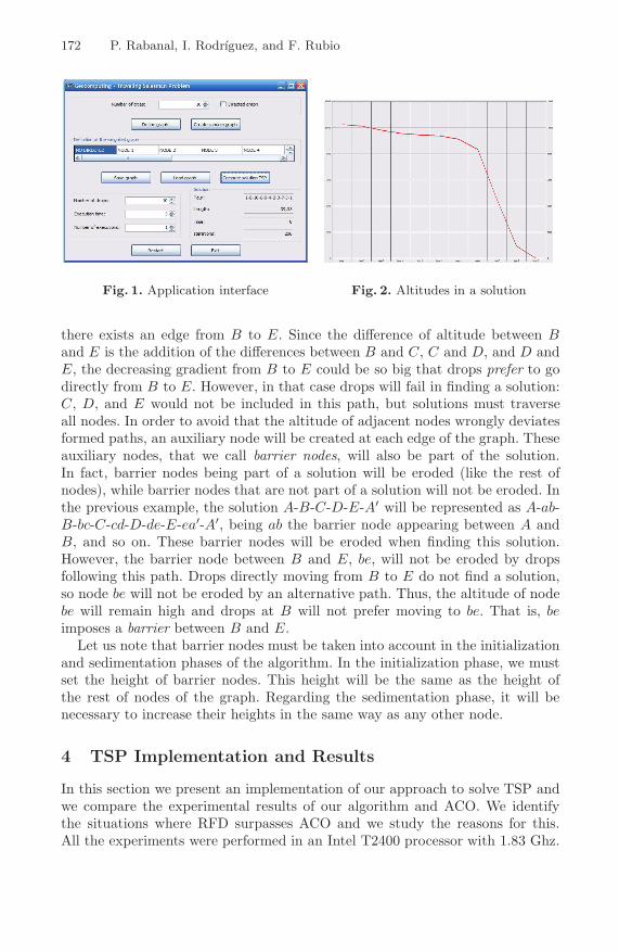
172 P. Rabanal, I. Rodrıguez, and F. Rubio
Fig. 1. Application interface Fig. 2. Altitudes in a solution
there exists an edge from B to E. Since the difference of altitude between Band E is the addition of the differences between B and C, C and D, and D andE, the decreasing gradient from B to E could be so big that drops prefer to godirectly from B to E. However, in that case drops will fail in finding a solution:C, D, and E would not be included in this path, but solutions must traverseall nodes. In order to avoid that the altitude of adjacent nodes wrongly deviatesformed paths, an auxiliary node will be created at each edge of the graph. Theseauxiliary nodes, that we call barrier nodes, will also be part of the solution.In fact, barrier nodes being part of a solution will be eroded (like the rest ofnodes), while barrier nodes that are not part of a solution will not be eroded. Inthe previous example, the solution A-B-C-D-E-A′ will be represented as A-ab-B-bc-C-cd-D-de-E-ea′-A′, being ab the barrier node appearing between A andB, and so on. These barrier nodes will be eroded when finding this solution.However, the barrier node between B and E, be, will not be eroded by dropsfollowing this path. Drops directly moving from B to E do not find a solution,so node be will not be eroded by an alternative path. Thus, the altitude of nodebe will remain high and drops at B will not prefer moving to be. That is, beimposes a barrier between B and E.
Let us note that barrier nodes must be taken into account in the initializationand sedimentation phases of the algorithm. In the initialization phase, we mustset the height of barrier nodes. This height will be the same as the height ofthe rest of nodes of the graph. Regarding the sedimentation phase, it will benecessary to increase their heights in the same way as any other node.
4 TSP Implementation and Results
In this section we present an implementation of our approach to solve TSP andwe compare the experimental results of our algorithm and ACO. We identifythe situations where RFD surpasses ACO and we study the reasons for this.All the experiments were performed in an Intel T2400 processor with 1.83 Ghz.

Using River Formation Dynamics 173
Fig. 3. Results for a 20 (left) and 30 (right) nodes random graph
Fig. 4. Results for the TSPLIB eil51 graph
Figure 1 shows the interface of the application we developed to implement bothmethods and Figure 2 depicts an example of solution found by RFD. It showsthe altitudes of the nodes of the path in the order they are traversed.
Let us present our experimental results. Figure 3 (left) shows the results of anexperiment where the input of both algorithms was a given randomly generatedgraph with 20 nodes. The graphic shows the best solution found by each algo-rithm for each execution time. Figure 3(right) shows the results obtained afterapplying both methods to a random graph with 30 nodes. Next, in Figure 4we show the results obtained for a graph taken from the TSPLIB library [12].TSPLIB is a library of sample instances for TSP from various sources and ofvarious types. Nodes are defined by means of points in a 2D plain and there isan edge between all pairs of nodes. The distance of each edge is the Euclideandistance between both points of the plain. Figure 4 shows the results after apply-ing the graph eil51 from TSPLIB (with 51 nodes) to both methods. The basicshape shown in the figure is usually obtained with more benchmark examples.
Before we analyze the results shown in these figures, let us comment on howthe ACO approach and the RFD approach were compared in each experiment.The number of ants in ACO and the number of drops in our approach does notcoincide in each experiment. For each graph, we analyzed the number of ants

174 P. Rabanal, I. Rodrıguez, and F. Rubio
(respectively drops) that provided the best solutions in the ACO algorithm (resp.in RFD). We observed that the optimal number of entities traversing each graphwas different in both approaches. For example, for the graph with 51 nodes,the number of ants was set to one thousand and the number of drops was setto one hundred because we observed that one thousand and one hundred werethe optimal choices for each method. Let us note that moving an ant does notrequire exactly the same computational effort than moving a drop. Moreover,the effect caused by moving each of them in terms of its partial contribution tofuture solutions (i.e., in terms of higher pheromone trails and lower altitudes,respectively) is different. Since both entities are not comparable, assessing theperformance of both algorithms with the same number of populations is notappropriate. On the contrary, we compare both methods by applying the optimalpopulation in each case.
We extract the following conclusions from the experimental results. We ob-serve that ACO provides good solutions in short times. This is because ants tendto converge through the same path in short times. On the other hand, the solu-tions found by RFD after short execution times are poor. However, after sometime, the quality of the solutions of the RFD method surpasses the quality of thesolutions provided by ACO. That is, the convergence of drops is achieved laterthan the convergence of ants, but better paths are traversed by drops. Hence,RFD is the best choice if the quality of the solutions is more important than thetime needed to achieve them.
There are several reasons for this difference in both approaches. First, let usnote that slopes formed by drops tend to form a general movement tendencyfor subsequent drops. This tendency leads drops from the origin node to itself(in our method, to its clone) in an established direction. It is similar to thecase that we take a Billiard table and we gradually tilt it towards a cornerpocket. This tendency allows drops to homogeneously explore the graph aftersome iterations, that is, edges are explored regardless of their distance to theorigin/destination node. However, this general tendency is lower in ACO meth-ods because pheromone trails in edges do not impose a given direction to ants.If an edge from A to B has a high pheromone trail then ants at A try to go to B,and ants at B tend to go to A. Hence, general tendencies to explore the graphare more difficult to create, and ants tend to cumulate themselves in specificlocal areas because the exploration of each zone feeds itself back. This allows toimprove the exploration of areas already traversed, but makes it more difficultto explore other alternative zones. The result is that the convergence is fasterin the ACO method than in RFD, but the solutions found by ACO are worsebecause the exploration is focalized.
Another reason for this behavior is related to the way a new shortcut isreinforced in our method. As we already commented in previous sections, whena shorter path is found by drops, it is easy for subsequent drops to reinforcethis path until it is preferred in all cases to other choices. This is because thenew path is actually attractive for other drops from the time the reinforcementbegins. We could argue that, if shorter paths are reinforced quickly, then the

Using River Formation Dynamics 175
preference of drops for short paths would accelerate their convergence on thecost of ignoring other paths that are bad in the short term (but may be good inthe long term). That is, we have a reason to obtain an opposite behavior to theone commented before. However, we observed the following behavior: Since shortpaths quickly become attractive choices, it is usual that, at the same time, thereare several new attractive choices challenging older longer paths. As long as thesenew alternative paths confront each other, drops have several attractive choicesto move next. This enables a deeper exploration of the graph (and, paradoxically,a slower overall convergence).
The way in which we handle the sedimentation in RFD also favors this behav-ior. Recall that we allow drops to deposit sediments in blind alleys. Eventuallythis fills the hole, which avoids that other drops follow the same wrong path. Asa consequence, drops perform a try and fail mechanism where new paths are it-eratively formed/blocked until good paths are found. This also enables a deeperexploration of the graph, leading to better solutions and longer execution times.
As we commented in previous sections, our method avoids in practice thatdrops follow local cycles, which would lead to situations where all edges avail-able from a node connect to repeated nodes. Being provided with an intrinsicmethod to avoid the repetition of nodes (in our case, the difference of altitudes)lets drops spread around the graph, which also improves the exhaustivenessof the exploration. However, the main consequence of this characteristic is thefollowing: The number of drops that must be eliminated because they lead torepeated nodes is lower than the number of ants that must be eliminated for thesame reason.
Let us note that in RFD drops are also eliminated when all adjacent nodesare higher than the current node. Thus, there is a reason to eliminate dropsin RFD that does not exist in ACO. However let us note that, when a drop isblocked in a valley, the drop deposits its sediment. That is, the drop contributesto transform the graph values and its existence is actually useful for subsequentdrops. On the other hand, a blocked ant is useless for the method because itdisappears without modifying any pheromone trail (note that an ant modifiestrails only when it finds a solution). Hence, the computational effort spent tomove it was lost.
5 Conclusions and Future Work
In this paper we have presented a new heuristic method to solve complex prob-lems. The method is inspired on the way rivers are created in nature. By usingit, we can obtain acceptable solutions to NP-hard problems in reasonable times.Our method obtains competitive results when compared with other more ma-tured schemes, like ants colonies. In the TSP case study, our current experimentalresults shows that the RFD method is preferable to ACO if the optimality ofthe solution is the main requirement. The fast reinforcement of shortcuts, theavoidance of local cycles, the punishment of wrong paths, and the creation ofglobal direction tendencies motivate these results.

176 P. Rabanal, I. Rodrıguez, and F. Rubio
Our current lines of work are divided in two parts. First, we are working onoptimizing our basic scheme. For instance, we may consider the following newdirections of improvement: Masses of water could be considered as part of thealtitude of nodes (currently, only the altitude of the ground is considered); thenumber of drops moved across the environment, which currently is constant fromthe first step, could vary along the execution depending on the convenience ofparallel/focused exploration; in order to improve the mechanism to avoid wrongpaths, sediments could be deposited not only in standard nodes but also inbarrier nodes; an hybrid ants/drops approach, where the weight of each methodvaries along the execution, could be constructed. This would allow to get thebest characteristics of each method in a single approach.
Second, we are also applying RFD to solve a wider set of problems. First, weare considering the exploration of dynamic graphs, that is, graphs where edgesmay appear and disappear along time. We have reasons to expect that this will bea suitable application case for our method. If an old path is suddenly blocked thenthe sedimentation mechanism and the way in which shortcuts are reinforced willallow drops to quickly avoid the blocked path and find alternatives. In addition,we want to explore the problem of finding optimal grouped solutions from severalorigins to a single destination. As we commented in the introduction, rivers donot follow optimal paths from a single point to the sea. On the contrary, theyoptimize the task of gathering and transporting the water from each point whereit rains (i.e., millions of departure points) to the sea through a grouped path.Following this idea, we can apply RFD to the problem of finding optimal pathsfor public transportation lines, that is, to decide the best path to gather andtransport population from residential areas to e.g. the city center.
Acknowledgments
We would like to thank the anonymous reviewers for valuable comments on aprevious version of this paper. Moreover, we would also like to thank ManuelNunez and Natalia Lopez for interesting discussions on the topic of the paper.
References
1. Applegate, D.L., Bixby, R.E., Chvatal, V., Cook, W.J.: The Traveling Sales-man Problem: A Computational Study. Princeton University Press, Princeton,NJ (2006)
2. Davis, L. (ed.): Handbook of genetic algorithms. Van Nostrand Reinhold, NewYork (1991)
3. Dorigo, M.: Ant Colony Optimization. MIT Press, Cambridge (2004)
4. Dorigo, M., Gambardella, L.M.: Ant colonies for the traveling salesman problem.BioSystems 43(2), 73–81 (1997)
5. Dorigo, M., Maniezzo, V., Colorni, A.: Ant system: optimization by a colony ofcooperating agents. IEEE Transactions on Systems, Man and Cybernetics, PartB 26(1), 29–41 (1996)

Using River Formation Dynamics 177
6. Fleischer, M.: Simulated annealing: past, present, and future. In: Proceedings ofthe 27th conference on Winter simulation, pp. 155–161 (1995)
7. Gutin, G., Punnen, A.P.: The Traveling Salesman Problem and Its Variations.Kluwer Academic Publishers, Dordrecht (2002)
8. Haupt, R.L., Haupt, S.E.: Practical Genetic Algorithms. Wiley-Interscience, NewYork, NY, USA (2004)
9. Kennedy, J., Eberhart, R.: Particle swarm optimization. In: Proceedings of IEEEInternational Conference on Neural Networks, 1995, vol. 4 (1995)
10. Kirkpatrick, S., Gelatt, Jr., C.D., Vecchi, M.P.: Optimization by Simulated An-nealing. Science 220(4598), 671 (1983)
11. Langton, C.: Studying artificial life with cellular automata. Physica D 22, 120–149(1986)
12. Reinelt, G.: TSPLIB 95. Technical report, Research Report, Institut fur Ange-wandte Mathematik, Universitat Heidelberg, Heidelberg, Germany (1995),http://www.iwr.uni-heidelberg.de/groups/comopt/software/TSPLIB95/
13. Rosenberg, G., Salomaa, A. (eds.): Lindenmayer Systems: Impacts on Theoreti-cal Computer Science, Computer Graphics, and Developmental Biology. Springer,Heidelberg (1992)
14. Wolfram, S.: Cellular Automata and Complexity. Addison-Wesley, London, UK(1994)

Principles of Stochastic Local Search
Uwe Schoning
Institute of Theoretical Computer ScienceUlm University
89069 Ulm, [email protected]
Abstract. We set up a general generic framework for local searchalgorithms. Then we show in this generic setting how heuristic, problem-specific information can be used to improve the success probability of lo-cal search by focussing the search process on specific neighbor states. Ourmain contribution is a result which states that stochastic local search us-ing restarts has a provable complexity advantage compared to determin-istic local search. An important side aspect is the insight that restarting(starting the search process all over, not using any information computedbefore) is a useful concept which was mostly ignored before.
Keywords: local search, stochastic local search, heuristic information,restart, meta-algorithmics.
1 Introduction
As compared to standard algorithm design techniques, local search algorithmsperform a quite unconventional computation since in most cases the problem-specific evaluation function (for example, the number of unsatisfied constraints,the length of the TSP tour found so far, etc.) can only give a weak guidanceinformation regarding what is the best direction for choosing the next localsearch step. Therefore, especially to escape the situation of getting stuck in localoptima, up to a certain amount, randomness is used to give the search processthe chance to find a way out of “dead ends.” But randomness alone (so-called“uninformed search”) does not help either, and is a poor strategy.
In this work we set up a general framework for modelling local search algo-rithms (which is more or less the standard one.) Then, under the assumption,that problem-specific (“heuristic”) information about the problem in question isavailable which allows to focus the search on a certain well-chosen subset of theneighbors of a state, a rigorous probabilistic analysis of local search is possible.The master example where such heuristic information indeed is available, is SAT,or k-SAT. But also for other types of problems this approach might be applica-ble. Our analysis results in precise probability estimations for finding a solution,and shows that stochastic local search has a provable complexity advantage as
S.G. Akl et al.(Eds.): UC 2007, LNCS 4618, pp. 178–187, 2007.c© Springer-Verlag Berlin Heidelberg 2007

Principles of Stochastic Local Search 179
compared to deterministic (backtracking-like) local search. An additional out-come of the analysis is that it is much better to restart the search process severaltimes, just after a few unsuccessful local search steps, than to continue the lo-cal search process towards the stationary (Markov chain) distribution. This isin contrast to many text book opinions where one can find the statement thatrestarting a local search process is usually a “poor strategy.”
2 Modelling Local Search Algorithms
The following first definitions are standard when modelling the scenario of localsearch (see e.g. [1,8,9,10,13].)
Definition. A local search scenario for a combinatorial decision (or optimizationproblem) Π is given by the following components. Given an input instance π,one can associate with π the following items
– a search space S. The elements of S are called candidate solutions or states,– a set S0 ⊆ S of (optimal) solutions,– a neighborhood relation N ⊆ S × S. (We sometimes use N in unary (func-
tional) form so that N(x) denotes the set of all y such that (x, y) ∈ N .)– the solution distance d(x) of a state x ∈ S is defined by
d(x) = min {k | ∃x1, . . . , xk∈S :
(x, x1)∈N, (x1, x2)∈N, . . . , (xk−1, xk)∈N, xk ∈S0}
Example. The well known problem SAT is, given a formula π in propositionallogic, find an assignment a for the Boolean variables occuring in π which satisfiesformula π. Let the formula π have n Boolean variables. Then the candidatesolutions are all the possible assignments to these variables. As it is often thecase, the candidate solutions, the elements of the search space S, can be dividedinto n components a = (a1, a2, . . . , an), ai ∈ {0, 1}. For each component thereare, in this case, two possible selections, namely, 0 and 1. (For more generalconstraint satisfaction problems there might be more selections per component.)Therefore, in this case, the search space is S = {0, 1}n, and |S| = 2n. Thesolution set is S0 = {a ∈ S | a satisfies π}. Two assignments a, a′ are neighborsof each other, i.e. (a, a′) ∈ N , and (a′, a) ∈ N , if and only if they differ inexactly one component. In other words, if their Hamming distance is 1. Thesolution distance of an assignment a is the minimal number of bits that haveto be flipped to arrive at a satisfying assignment. This is the smallest possiblenumber of local search steps, starting from x, that might lead to a solution.
The above definitions are specific to the respective problem Π (although forthe same problem Π there might be several useful definitions of the state spaceand the neighborhood relation.) More towards the design of a particular local
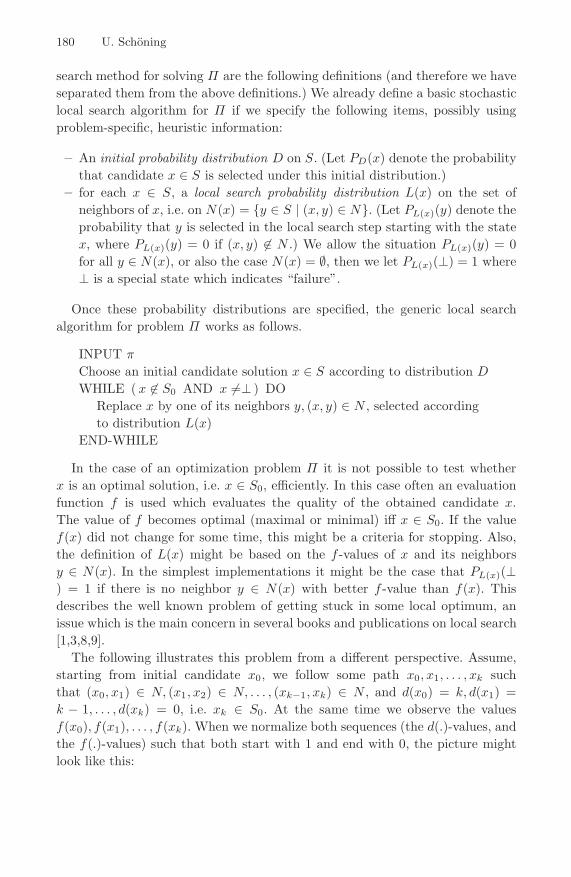
180 U. Schoning
search method for solving Π are the following definitions (and therefore we haveseparated them from the above definitions.) We already define a basic stochasticlocal search algorithm for Π if we specify the following items, possibly usingproblem-specific, heuristic information:
– An initial probability distribution D on S. (Let PD(x) denote the probabilitythat candidate x ∈ S is selected under this initial distribution.)
– for each x ∈ S, a local search probability distribution L(x) on the set ofneighbors of x, i.e. on N(x) = {y ∈ S | (x, y) ∈ N}. (Let PL(x)(y) denote theprobability that y is selected in the local search step starting with the statex, where PL(x)(y) = 0 if (x, y) �∈ N .) We allow the situation PL(x)(y) = 0for all y ∈ N(x), or also the case N(x) = ∅, then we let PL(x)(⊥) = 1 where⊥ is a special state which indicates “failure”.
Once these probability distributions are specified, the generic local searchalgorithm for problem Π works as follows.
INPUT π
Choose an initial candidate solution x ∈ S according to distribution DWHILE ( x �∈ S0 AND x �=⊥ ) DO
Replace x by one of its neighbors y, (x, y) ∈ N , selected accordingto distribution L(x)
END-WHILE
In the case of an optimization problem Π it is not possible to test whetherx is an optimal solution, i.e. x ∈ S0, efficiently. In this case often an evaluationfunction f is used which evaluates the quality of the obtained candidate x.The value of f becomes optimal (maximal or minimal) iff x ∈ S0. If the valuef(x) did not change for some time, this might be a criteria for stopping. Also,the definition of L(x) might be based on the f -values of x and its neighborsy ∈ N(x). In the simplest implementations it might be the case that PL(x)(⊥) = 1 if there is no neighbor y ∈ N(x) with better f -value than f(x). Thisdescribes the well known problem of getting stuck in some local optimum, anissue which is the main concern in several books and publications on local search[1,3,8,9].
The following illustrates this problem from a different perspective. Assume,starting from initial candidate x0, we follow some path x0, x1, . . . , xk suchthat (x0, x1) ∈ N, (x1, x2) ∈ N, . . . , (xk−1, xk) ∈ N , and d(x0) = k, d(x1) =k − 1, . . . , d(xk) = 0, i.e. xk ∈ S0. At the same time we observe the valuesf(x0), f(x1), . . . , f(xk). When we normalize both sequences (the d(.)-values, andthe f(.)-values) such that both start with 1 and end with 0, the picture mightlook like this:

Principles of Stochastic Local Search 181
�
�
��
��
��
��
��
��
��
��
1
00 k
d
f�
������������
���
This means, except from the starting and ending point and a general ten-dency there are only few similarites between both curves. On the other hand, tocompute the function d(x) exactly is just as hard as solving the original problemΠ . If we could calculate d(y) exactly for all the neighbors of x we can select thatone which minimizes the solution distance.
Example. In the SAT example mentioned above, a natural (and often used)way to define f(x) for an assignment x, and a given formula π in conjunctivenormal form (clause form) is to let
f(x) = number of unsatisfied clauses in π under assignment x
Indeed, as the above figure indicates, there is not very strong correlation betweenf(x) and the solution distance d(x).
A direct, naive way of defining the inititial distribution for SAT is to assign eachassignment x ∈ {0, 1}n the same probability, PD(x) = 2−n. A similar direct wayof defining the local search probability is to assign each neighbor of x the sameprobability, i.e.
PL(x)(y) ={
1/n, if y ∈ N(x),0, otherwise
This does not result in a good local search algorithm. The probability that such arandom local search step according to distribution L(x) will decrease the solutiondistance is d(x)/n, that is, the closer x is to the desired solution, the harder isit to come even closer.
3 Heuristic Information and Markov Chain Analysis
In [11,15,16], in the case of k-SAT, a different local search probability distributionis used. This restricted neighborhood can be understood as bringing in some

182 U. Schoning
problem-specific heuristic information. Given an assignment x which does notyet satisfy the k-CNF formula π, there will be at least one clause in π which isnot satisfied. Let σ be one (e.g. the first) such clause. The clause σ contains kvariables (negated or non-negated). Let Nσ(x) be the subset of N(x) of size kwhich contains those neighbors of x where exactly one bit of x is flipped andthis bit belongs to a variable in σ. We let
PL(x)(y) ={
1/k, if y ∈ Nσ(x),0, otherwise
In this case, using L(x) for a local search step, the probability of decreasing d(x)by 1 is (at least) 1/k (since in a satisfying assignment there should at least oneof the k bits be flipped to satisfy the clause σ), and this is better than the abovenaive approach once the solution distance d(x) is at most n/k. Indeed, as shownin [11], the expected number of local search steps until a solution is found, isquadratic in n, in the case of 2-SAT. The case k > 2 is handled in [15,16]. Theprobability that a single run of 3n local search steps will find a solution is shownto be at least 1
p(n) · ( k2k−2 )n where p is some (small) polynomial.
It is clear that this basis version of a local search algorithm will only besuccessful with some probability, depending on the choice of D and L(x), asindicated by the SAT example above. Therefore, it is a good idea to restartthe basis algorithm several times with independent new initial solution candi-dates. This is realized in the following program (here t is some parameter whichindicates the number of local search steps until to restart.)
INPUT π
REPEAT FOREVERChoose an initial candidate solution x ∈ S according todistribution D; set i := 0WHILE (x �∈ S0 AND x �=⊥ AND i ≤ t ) DO
i := i+ 1Replace x by one of its neighbors y, (x, y) ∈ N ,selected according to distribution L(x)
END-WHILEIF x ∈ S0 THEN STOP successfully
REPEAT-END
The behavior of this stochastic local search algorithm can be understood asa Markov chain in the following way.
We can understand the probability distribution D as a vector of length |S|.By [D]x we indicate the component indexed by x ∈ S in D, i.e. [D]x = PD(x).
Similarly, we can understand the set of all L(x) for x ∈ S as a |S| × |S|stochastic matrix, denoted ML, where the (x, y)-th entry in this matrix ML
denotes the probability PL(x)(y).

Principles of Stochastic Local Search 183
The result of the t-fold vector-matrix multiplication D · (ML)t is a vectorof length |S|. The component indexed by x ∈ S indicates the probability thatstate x is reached after the initial random choice followed by t local search steps.Therefore, the “success probability”, the probability of reaching a solution withinone run of the REPEAT-loop, is given by
p =∑x∈S0
[D · (ML)t]x
If we could calculate or estimate p (which is quite difficult), then an appropriatenumber of restarts (number of REPEAT-loops) would be c/p for some con-stant c. This is so, since the probability of missing a solution in each of the c/ptrials is
(1 − p)c/p ≤ (e−p)c/p = e−c
It is difficult to calculate p since the respective vector D and the matrix ML
are exponential in the size of π, and both, D and ML, depend individually onthe input instance π. We could greatly simplify the analysis, if
– it is possible that the complexity analysis depends merely on the input sizen = |π|, and not on π itself,
– if the number of states of the Markov chain (that is, the vector D, and thematrix ML) can be reduced.
These requirements can indeed be fulfilled if we divide the search space S (theset of states) into a few categories (equivalence classes), like
S = S0 + S1 + · · · + Sn
and we base the Markov chain (and its analysis) on these “super states”. A quitenatural division of S into categories is in terms of the solution distance. Define
Si = {x ∈ S | d(x) = i}
Example. Continuing the above SAT example it can be seen, that a Markovchain approach using the “super states” 0, 1, . . . , n, indicating the solution dis-tance d(x) of the actual assignment x, can be used. Consider the case of k-SAT,and let Yt be a random variable describing the state number at time t. Then Y0
is determined by the initial distribution D:
P (Y0 = j) =(n
j
)2−n
The transition probabilities from time t to time t+ 1 are as follows.
P (Yt+1 = j − 1 | Yt = j) =1k
and P (Yt+1 = j + 1 | Yt = j) =k − 1k

184 U. Schoning
Let q(t, j) = P (Yt = 0 | Y0 = j), i.e. the probability that the state 0 (whichindicates that a solution is found) is reached after exactly t steps, under thecondition that the initial solution distance is j. Clearly, we have q(t, j) = 0 fort < j. For t = j we have q(t, j) = ( 1
k )j , and in the general case, t > j, lettingt = (1 + α)j, we get (using the ballot theorem, cf. [6]),
q((1 + α)j, j) =(
(1 + α)jαj/2
)· 11 + α
·((k − 1k
)α/2 · ( 1k
)1+α/2)j
Asymptotically, and concentrating on the exponential terms, we can approximatethis probability as follows.
q((1 + α)j, j) ≈[2h( α
2(1+α) )(1+α) · (k − 1k
)α/2 · ( 1k
)1+α/2]j
=: βj
where h is the binary entropy function [2]. The following figure shows β as afunction of α.
�
� α
β
0 2k−2
1k
1k−1
In the beginning (i.e. α = 0, that is, t = j) we have β = 1/k, but the highestvalue, β = 1/(k−1) is reached later when α = 2/(k−2), that is, t = j ·k/(k−2).We find this quite surprising. It shows an advantage of stochastic local searchas compared to deterministic local search, which, in this case would explore thestates, starting from the initial state x up to states within Hamming distance j.Then a solution would be found. Doing this systematic search in a backtrackingfashion (as in [14,4,5]) requires kj search steps (= recursive calls of the searchprocedure), whereas the probability of finding the solution in a single run ofstochastic search of at least j · k/(k− 2) (not just j) steps is (1/(k− 1))j . UsingO((k−1)j) restarts, as explained above, this results in an algorithm which findsthe solution (of distance j) almost surely.
4 Restarts
To make the discussion complete, we need to combine this analysis of the localsearch process (given that the solution distance is j) with the initial randomdistribution D. Altogether we combine a random initial choice of a solution

Principles of Stochastic Local Search 185
candidate, followed by at least j · k/(k− 2) local search steps according to L(x).Since we don’t know the particular j in advance, we can use the upper boundn · k/(k− 2) for the number of local search steps before to restart. The resultingsuccess probability is
n∑j=0
(n
j
)· 2−n · ( 1
k − 1)j = (
k
2k − 2)n
by the binomial theorem. Let r(t) be the probability that we reach a solutionafter exactly t local search steps, following the initial guess of a candidate. Thenthis function reaches its maximum at t = n/(k − 2), where this maximum valueconicides, up to polynomial factors, with the above, namely βn = ( k
2k−2 )n. Thefollowing picture indicates the situation.
�
� t
β
0 nk−2
r(t)1/nk
2k−2
Now it should be clear that it is not the best strategy to make just a singlerun of the local search algorithm until eventually a solution is reached. Apartfrom these theoretical results, experiments with this “pure random walksat”procedure, as reported in [12], page 99ff, or in [7], page 258ff, suggest that thealgorithm becomes trapped in a “metastable state” for a very long time, anddoes not reach the solution during this phase. Therefore, a much better strategyis to restart after t0 > n
k−2 steps if no solution was found so far. This strategyresults in a picture like the following.
� t
β
0 nk−2 t0 2t0
�

186 U. Schoning
In the first phase, for 0 ≤ t ≤ t0, let the probability of finding a solution be p(up to a polynomial factor we have p = ( k
2k−2 )n). Then the probability of findinga solution, not in the first, but in the second phase, is (1− p) · p, and in general,for the i-th phase, (1−p)i−1 ·p. These probabilities are much greater than in theabove situation (without any restart), which are, up to some polynomial factor,r(t0), r(2t0), . . ..
Usually, when using a Markov chain approach to analyze a random algorithmit is the issue of rapid mixing which is of concern, i.e. reaching the stationarydistribution quickly. It is interesting to note that the situation here is quite dif-ferent. The probability of finding a solution is highest within a certain initialnumber of steps, afterwards when reaching the stationary distribution, it de-creases drastically. Therefore, restarting is an important concept here which, inour opinion, has been neglected so far.
Acknowledgement
I would like to thank Hans Kestler for many productive and intuitive discussionson the subject.
References
1. Aarts, E., Lenstra, J.K.: Local Search in Combinatorial Optimization. PrincetonUniversity Press, Princeton, NJ (2003)
2. Ash, R.B.: Information Theory. Dover, Mineola, NY (1965)3. Bolc, L., Cytowski, J.: Search Methods for Artificial Intelligence. Academic Press,
San Diego (1992)4. Dantsin, E., Goerdt, A., Hirsch, E.A., Schoning, U.: Deterministic algorithms for k-
SAT based on covering codes and local search. In: Welzl, E., Montanari, U., Rolim,J.D.P. (eds.) ICALP 2000. LNCS, vol. 1853, pp. 236–247. Springer, Heidelberg(2000)
5. Dantsin, E., Goerdt, A., Hirsch, E.A., Kannan, R., Kleinberg, J., Papadimitriou,C., Raghavan, P., Schoning, U.: A deterministic (2 − 2
k+1)n algorithm for k-SAT
based on local search. Theoretical Computer Science 289(1), 69–83 (2002)6. Feller, W.: An Introduction to Probability Theory and Its Applications. Wiley,
Chichester (1968)7. Hartmann, A.K., Weigt, M.: Phase Transitions in Combinatorial Optimization
Problems. Wiley-VHC, Chichester (2005)8. Hoos, H.: Stochastic Local Search - Methods, Models, Applications. PhD disserta-
tion, Universitat Darmstadt (1998)9. Hoos, H., Stutzle, T.: Stochastic Local Search - Foundations and Applications.
Morgan Kaufmann, San Francisco (2004)10. Michiels, W., Aarts, E., Korst, J.: Theoretical Aspects of Local Search. Springer,
Heidelberg (2007)11. Papadimitriou, C.H.: On selecting a satisfying truth assignment. In: Proceedings
of the 32nd Ann. IEEE Symp. on Foundations of Computer Science, pp. 163–169.IEEE Computer Society Press, Los Alamitos (1991)

Principles of Stochastic Local Search 187
12. Perkus, A., Istrate, G., Moore, C. (eds.): Computational Complexity and StatisticalPhysics. Oxford University Press, Oxford (2006)
13. Schneider, J.J., Kirkpatrick, S.: Stochastic Optimization. Springer, Heidelberg(2006)
14. Schoning, U.: On The Complexity Of Constraint Satisfaction Problems. UlmerInformatik-Berichte, Nr. 99-03. Universitat Ulm, Fakultat fur Informatik (1999)
15. Schoning, U.: A probabilistic algorithm for k-SAT and constraint satisfaction prob-lems. In: Proceedings 40th IEEE Symposium on Foundations of Computer Science,pp. 410–414 (1999)
16. Schoning, U.: A probabilistic algorithm for k-SAT based on limited local searchand restart. Algorithmica 32(4), 615–623 (2002)

S.G. Akl et al.(Eds.): UC 2007, LNCS 4618, pp. 188–198, 2007. © Springer-Verlag Berlin Heidelberg 2007
Spatial and Temporal Resource Allocation for Adaptive Parallel Genetic Algorithm
K.Y. Szeto
Department of Physics Hong Kong University of Science and Technology,
Clear Water Bay, Hong Kong, SAR, China {[email protected]}
Abstract. Adaptive parameter control in evolutionary computation is achieved by a method of computational resource allocation, both spatially and tempo-rally. Spatially it is achieved for the parallel genetic algorithm by the partition-ing of the search space into many subspaces. Search for solution is performed in each subspace by a genetic algorithm which domain of chromosomes is re-stricted inside that particular subspace. This spatial allocation of computational resource takes the advantage of exhaustive search which avoids duplicate effort, and combine it with the parallel nature of the search for solution in disjoint sub-spaces by genetic algorithm. In each subspace, temporal resource allocation is also made for different competing evolutionary algorithms, so that more CPU time is allocated to those algorithms which showed better performance in the past. This general idea is implemented in a new adaptive genetic algorithm us-ing the formalism of mutation matrix, where the need for setting a survival probability is removed. The temporal resource allocation is introduced and im-plemented in a single computer using the quasi-parallel time sharing algorithm for the solution of the zero/one knapsack problem. The mutation matrix ( )M t is constructed using the locus statistics and the fitness distribution in a population
( )A t with N rows and L columns, where N is the size of the population and L is the length of the encoded chromosomes. The mutation matrix is parameter free and adaptive as it is time dependent and captures the accumulated information in the past generation. Two competing strategies of evolution, mutation by row (chromosome), and mutation by column (locus) are used for the competition of CPU time. Time sharing experiment on these two strategies is performed on a single computer in solving the knapsack problem. Based on the investment frontier of time allocation, the optimal configuration in solving the knapsack problem is found.
1 Introduction
Successful applications of genetic algorithm using the Darwinian principle of survival of the fittest have been implemented in many areas [1,2], such as in solving the crypto-arithmetic problem [3], time series forecasting [4], traveling salesman problem [5], function optimization [6], and adaptive agents in stock markets [7,8]. A drawback for the practitioners of genetic algorithm is the need for expertise in the specific

Spatial and Temporal Resource Allocation for Adaptive Parallel Genetic Algorithm 189
application, as its efficiency depends very much on the parameters chosen in the evolutionary process. An example of this drawback can be found in the ad-hoc man-ner in choosing the selection mechanism, where different percentages of the popula-tion for survival for different problems are generally required. Since the parameters used in a specific application will usually not be optimal in a different application, the traditional usage of genetic algorithm is more like an artisan approach. To tackle this shortcoming, we attempt an adaptive approach where the number of parameters re-quiring input from experts is reduced to a minimum. The basic aim is to make use of past data collected in the evolutionary process of genetic algorithm to tune the pa-rameters such as the survival probability of a chromosome. In this paper we provide a general framework for adaptive parameter control for parallel genetic algorithm, both spatially and temporally.
Temporally we can collect the statistics of the chromosomes in past generations to decide the probability of mutation of each locus [9]. A general formalism using a mutation matrix has been introduced with generalization to adaptive crossover mechanism reported in a recent publication [10,11], which was reviewed briefly in Section 2. Here we emphasize not only the adaptive parameter control in a particular algorithm of evolutionary computation, but also the competition among several adap-tive algorithms for computational time, assuming that there is a single CPU available. This competition of CPU time then addresses the problem of adaptive temporal allo-cation of resource to individual algorithm by a quasi-parallel process, which is sto-chastic in nature [12]. To illustrate this problem in layman’s terms, let’s consider two students, Alice and Bob, working independently on a difficult problem in cryptogra-phy. The Professor only provides one computer for them. Without knowing who is the better student, the professor gives Alice and Bob equal time sharing for the use of the computer. However, after some time, Alice shows more promising results. Thus, it is wise for the professor to give her more time to use the computer. A more sophisti-cated professor will then measure the risk of giving all time to Alice, and adjust the probability of computer usage at a given time by Alice accordingly. The problem of temporal allocation of computer time to Alice and Bob therefore is a problem of port-folio management, when the probability distribution functions of finding a solution by Alice and by Bob should be used in an optimal way. An excellent method in portfolio management has been provided by Markowitz [13] to locate the optimal parameters in running the bottleneck program in a single computer that satisfies the criteria of both high speed and high confidence. These ideas in laymen terms have been imple-mented technically by Hogg and Huberman and collaborators [14] and Szeto and Jiang [12]. The formalism is basically one of quasi-parallel genetic algorithm, which is aimed at combining existing algorithms into new ones that are unequivocally pref-erable to any of the component algorithms using the notion of risk in economics [13]. Here we assume that only one computer is available and the sharing of resource is realized only in the time domain. The concept of optimal usage is defined economi-cally by the “investment frontier”, characterized by low risk and high speed to solu-tion. We will illustrate this idea in Section 3 where we combine the work on mutation only genetic algorithm and time sharing in the framework of quasi-parallel genetic algorithm. We test this approach on the 0/1 knapsack problem with satisfactory re-sults, locating the investment frontier for the knapsack problem.

190 K.Y. Szeto
Spatially, we consider a simple partitioning of the solution space into disjoint sub-spaces, so that we can perform parallel search in each subspace with adaptive genetic algorithm with temporal parameter control. Our idea is to combine the advantage of exhaustive search, which does not duplicate effort in search, with parallel genetic algorithm. There will be communication between populations in different subspaces, but there is no exchange of chromosomes and all evolutionary processes are restricted to a given subspace. In this way, the dimensionality of the solution space is reduced. However, this is the trivial advantage of spatial partition. The real advantage comes from the allocation of computational resource to those populations which in the past show more promise in finding the solution. In layman’s term, let’s consider the search for a lost key in the beach. One first partitions the beach area into giant grids, and perform parallel intelligent search in a given grid with the help of friends. By looking for characteristic traces of the lost key, one naturally should spend more time in searching in a grid where there are more traces. In Section 4, we put this simple idea in more technical terms and suggest a way for performance evaluation for the search process in individual subspace.
2 Mutation Matrix
In traditional simple genetic algorithm, the mutation/crossover operators are proc-essed on the chromosome indiscriminately over the loci without making use of the loci statistics, which has been demonstrated to provide useful information on mutation operator [9]. In our mutation matrix formalism, the traditional genetic algorithm can be treated as a special case. Let’s consider a population of N chromosomes, each of length L and binary encoded. We describe the population by a NxL matrix, with entry
( ), 1,..., ; 1,...,ijA t i N j L= = denoting the value of the jth locus of the ith chromosome.
The convention is to order the rows of A by the fitness of the chromosomes, ( ) ( )i kf t f t for i k≤ ≥ . Traditionally we divide the population of N chromosomes
into three groups: (1) Survivors who are the fit ones. They form the first 1N rows of
the population matrix A(t+1). Here 1 1N c N= with the survival selection ratio
10 1.c< < (2) The number of children is 2 2N c N= and is generated from the fit
chromosomes by genetic operators such as mutation. Here 2 10 1c c< < − is the sec-
ond parameter of the model. We replace the next 2N rows in the population matrix
A(t+1). (3) the remaining 3 1 2N N N N= − − rows are the randomly generated chro-
mosomes to ensure the diversity of the population so that the genetic algorithm con-tinuously explores the solution space.
In our formalism, we introduce a mutation matrix with elements ( ) ( ) ( ), 1,..., ; 1,...,ij i jM t a t b t i N j L≡ = = where 0 ( ), ( ) 1i ja t b t≤ ≤ are called the row
mutation probability and column mutation probability respectively. Traditional genetic algorithm with mutation as the only genetic operator corresponds to a time independent mutation matrix with elements ( ) 0ijM t ≡ for
11,...,i N= , ( ) (0,1)ijM t m≡ ∈ for

Spatial and Temporal Resource Allocation for Adaptive Parallel Genetic Algorithm 191
1 21,..., ,i N N= + and finally we have ( ) 1ijM t ≡ for 2 1,...,i N N= + . Here m is the
time independent mutation rate. We see that traditional genetic algorithm with muta-
tion as the only genetic operator requires at least three parameters: 1 2, , and N N m .
We first consider the case of mutation on a fit chromosome. We expect to mutate only a few loci so that it keeps most of the information unchanged. This corre-sponds to ``exploitation'' of the features of fit chromosomes. On the other hand, when an unfit chromosome undergoes mutation, it should change many of its loci so that it can explore more regions of the solution space. This corresponds ``exploration''. Therefore, we require that ( )ijM t should be a monotonic increasing function of the
row index i since we order the population in descending order of fitness. There are many ways to introduce the row mutation probability. One simple solution is to use
( ) ( 1) /( 1)ia t i N= − − . Next, we must decide on the choice of loci for mutation once
we have selected a chromosome to undergo mutation. This is accomplished by com-puting the locus mutation probability of changing to X (X=0 or 1) at locus j as
jXp by
1 1
( 1 ) ( )N N
k jk m
jX N k X mp δ= =
= + −∑ ∑ (1)
Here k is the rank of the chromosome in the population. ( ) 1kj Xδ = if the j-th locus
of the k-th chromosome assume the value X, and zero otherwise. The factor in the
denominator is for normalization. Note that jXp contains information of both locus
and row and the locus statistics is biased so that heavier weight for chromosomes with high fitness is assumed. This is in general better than the original method of Ma and
Szeto[9] where there is no bias on the row. After defining jXp , we define the column
mutation rate as
( )0 1 '' 1
1 | 0 .5 | | 0 .5 |L
j j jj
j p p bb=
= − − − − ∑ (2)
For example, if 0 and 1 are randomly distributed, then 0 1 0.5j jp p= = . We have no
useful information about the locus, so we should mutate this locus, and 1jb = . When
there is definitive information, such as when 0 11 0 or 1j jp p= − = , we should not
mutate this column and 0jb = .
Once the mutation matrix M is obtained, we are ready to discuss the strategy of us-ing M to evolve A. There are two ways to do Mutation Only Genetic Algorithm. We can first decide which row (chromosome) to mutate, then which column (locus) to mutate, we call this particular method the Mutation Only Genetic Algorithm by Row or abbreviated as MOGAR. Alternatively, we can first select the column and then the row to mutate, and we call this the Mutation Only Genetic Algorithm by Column or abbreviated as MOGAC.

192 K.Y. Szeto
For MOGAR, we go through the population matrix A(t) by row first. The first step
is to order the set of locus mutation probability ( )jb t in descending order. This or-
dered set will be used for the determining of the set of column position (locus) in the mutation process. Now, for a given row i, we generate a random number x. If
( )ix a t< , then we perform mutation on this row, otherwise we proceed to the next
row and ( 1) ( ), 1,...,ij ijA t A t j L+ = = . If row i is to be mutated, we determine the
set ( )iR t of loci in row i to be changed by choosing the loci with ( )jb t in descending
order, till we obtain ( ) ( )i iK t a t L= ∗ members. Once the set ( )iR t has been con-
structed, mutation will be performed on these columns of the i-th row of the A(t) matrix to obtain the matrix elements ( 1), 1,...,ijA t j L+ = . We then go through all N
rows, so that in one generation, we need to sort a list of L probabilities ( )jb t and
generate N random numbers for the rows. After we obtained A(t+1), we need to com-
pute the ( 1) ( 1)ij i jM t a b t+ = + and proceed to the next generation.
For MOGAC, the operation is similar to MOGAR mathematically except now we rotate the matrix A by 90 degrees. Now, for a given column j we generate a random
number y. If ( )jy b t< , then we mutate this column, otherwise we proceed to the
next column and ( 1) ( ), 1,...,ij ijA t A t i N+ = = . If column j is to be mutated, we
determine the set ( )jS t of chromosomes in column j to be changed by choosing the
rows with the ( )ia t in descending order, till we obtain ( ) ( )j jW t b t N= ∗ members.
Since our matrix A is assumed to be row ordered by fitness, we simply need to choose
the , 1,..., 1jN N N W− − + rows to have the j-th column in these row mutated to
obtain the matrix elements ( 1), 1,...,ijA t i N+ = . We then go through all L columns,
so that in one generation, we need to sort a list of N fitness values and generate L random numbers for the columns.
3 Temporal Allocation of Resource
Our mutation matrix is adaptive and time dependent. The two strategies of using the mutation matrix formalism, MOGAR and MOGAC, present a good example for tem-poral allocation of computational resource. The framework for proper mixing of com-puting algorithms is the quasi-parallel algorithm of Szeto and Jiang [12]. Here we first summarize this algorithm. A simple version of our quasi-parallel genetic algorithm ( QPGA ( , , , )M SubGA T= Γ ) consists of M independent sub-algorithms SubGA. The
time sharing of the computing resource is described by the resource allocation vector Γ . If the total computing resource is R, shared by M sub-algorithms Gi, i=1,2,…,M, with resource Ri assigned to Gi in unit time, then we introduce

Spatial and Temporal Resource Allocation for Adaptive Parallel Genetic Algorithm 193
i iR Rτ = , 0 1iτ≤ ≤ for any i=1,2,…,M, and1
1M
iiτ
==∑ , and the allocation of re-
source for sub-algorithms is defined by the resource allocation vector,
1 2( , , )Mτ τ τ ′Γ = L . In our case, we have M=2 and our SubGA are MOGAR and
MOGAC. For resource allocation, we only have one parameter 0 1γ< < which is the
fraction of time the computer is using MOGAR, and the remaining fraction of time (1 γ− ) we use MOGAC. The termination criterion T is used to determine whether a
QPGA should stop running. Thus, we have a mixing of MOGAR with MOGAC in the framework of quasi-parallel genetic algorithm with a mixing parameter γ . The paral-
lel genetic algorithm described above can be implemented in a serial computer. For a particular generation t, we will generate a random number z. If z <γ , then we per-
form MOGAR, otherwise we perform MOGAC to generate the population A(t+1). We now apply this quasi-parallel mutation only genetic algorithm to solve the 0/1 knapsack problem and try to obtain the investment frontier that give the mixing pa-rameter γ that yields the fastest speed in solving the problem while also running with
most certainty (minimum risk) of getting the solution.
4 Spatial Allocation of Resource
Let’s begin with the simple case of binary encoding of the solution of a typical search problem for the maximum of a function. The quality of the solution is defined by the
length L of the chromosomes. In exhaustive search, we simply try all 2L chromo-somes in the solution space. If we partition the solution space into n subspaces,
{ }2 , (0 )kn k L= < < , we can perform intelligent search in each of these n sub-
spaces, so that there is an effective reduction in the dimension of search space from
2L to 2L k− . For example, we use n=4 and use the first two loci of the chromosomes:
( ) ( ){ }1... , (0,1); 1,..., ; , (0,1)cd k L iS cdx x x i k L c d+≡ ∈ = + ∈ . The four sets of
chromosomes ( )00 01 10 11, , ,S S S S describe typical solution restricted to the four sub-
spaces labeled by the first two loci. These subspaces are mutually exclusive so that search in each subspace can be performed independently without duplication of effort that often appears had the search not been restricted to individual subspace. Opera-tionally, one can search sequentially or randomly in these subspaces. For illustrative
purpose, we assume sequentially search in the order of ( )00 01 10 11, , ,S S S S by as-
signing four populations ( )00 01 10 11, , ,A A A A correspondingly for each of the sub-
space. In order to implement adaptive spatial allocation of resource, we evolve each
population ( )cdA for some generations ( )cdG . A time sharing process for the evolu-
tion of many populations with one CPU can then be implemented on these four popu-lations for the four subspaces. As in Section 3, we can do the allocation of CPU by the following steps:

194 K.Y. Szeto
1. Divide searching into segments with equal length τ which denotes the total num-ber of generations the program will evolve in all subspaces in the given segment.
2. Initialize each population with ( )00 01 10 11(0) (0) (0) (0) /G G G G nτ= = = = .
3. The population which represents a subspace with a higher probability to contain the global optimal solution will gain more computational time. The adaptive change of the sharing of resource can be done with a measure of the population
fitness ( )00 01 10 11, , ,F F F F of ( )00 01 10 11, , ,A A A A .
In this example, we need to define the population fitness, as well as a partition of the segment into n pieces for the n population to evolve in the next segment. Given a measure of population fitness, we can partition the segment by the monotonic increas-
ing function ( ( ))cd cdP F of population fitness so that the division of the segment time
is given by
00 00 01 01 10 10 11 11
( ( ))( 1)
( ( )) ( ( )) ( ( )) ( ( ))cd cd
cd
P F tG t
P F t P F t P F t P F tτ+ =
+ + + (3)
Here t is the label for the segment and initially, 1/cdP n= .
There are two remaining problems to be solved before one can use spatial resource
allocation. The first one concerns the function ( )cd cdP F . If we consider the evolving
populations ( )00 01 10 11, , ,A A A A representing states of a large system in different
configuration in the space of solutions, then they may be considered as the state of the system with specific “energy”, represented by their fitness values
( )00 01 10 11, , ,F F F F . The similarity of an evolving physical system with changing
energy landscape leads naturally to the Boltzmann form of FP e∝ . The partitioning of the segment τ accordingly follows the partition of unity of the Boltzmann factor in the canonical ensemble in statistical mechanics. Although this choice of the P is a heuristic one, it has the advantage of the interpretation of probability. However, even without appealing to physics, this choice for P in practice has the advantage of ampli-fying the effect of difference in population fitness, which is usually not large for prac-tical size of segment τ .
The second problem concerns the choice of F. Here we define F as the fitness of the population A in a given subspace S. For each member of the population A, which is a chromosome c, one can associate with c a fitness f. This fitness f is the usual definition of fitness in single population genetic algorithm. For example, if the prob-lem is to find the maximum of a given function H(x), then a trial solution x% can be represented as a binary string, which corresponds to the chromosome c in genetic algorithm. The fitness f of the chromosome can simply be ( )f H x= % . The popula-
tion fitness for a collection of N chromosomes can then be the average fitness of these N trial solutions. However, a better choice for population fitness is the maximum

Spatial and Temporal Resource Allocation for Adaptive Parallel Genetic Algorithm 195
fitness of the N solutions: max{ ( ); 1,..., }i iF f H x i N= = = . This is a better choice
for population fitness because our objective is to find the maximum of the H(x). In terms of performance evaluation, we can pose the following question: are we spending the effort to find the solution in the right place? By right place, we mean the subspace that actually contains the global maximum of H(x). Supposing that we partition the
solution space into four subspaces ( )00 01 10 11, , ,S S S S and that the global maximum
of H(x) is in cdS . If cdG G> , where ' '
' '
1c d
c d
G Gn
⎛ ⎞= ⎜ ⎟⎝ ⎠∑ is the average genera-
tion, then we can say that we are correctly devoting our search effort in the right place. Over a large number of numerical experiments that run this search for the
global maximum of H(x), the probability Q that cdG G> can be computed. This
probability Q represents the probability of correct spatial resource allocation in the search for maximum H(x) and it can be used as a measure of performance of the algo-rithm for the given choice of P and F.
5 The Zero/One Knapsack Problem
The model problem to test our ideas on resource allocation for adaptive genetic algo-rithm is the Knapsack problem. We define the 0/1 knapsack problem [15] as follow.
Given L items, each with profit iP , weight iw and the total capacity limit c, we need
to select a subset of L items to maximize the total profit, but its total weight does not exceed the capacity limit. Mathematically, we want to find the set
{0,1}, 1,...,ix i L∈ = to
1 1
Maximize subjected to constraintL L
j j j jj j
P x c w x= =
≥∑ ∑ (4)
We consider a particular knapsack problem with size L=150 items,
c=4000, [ ]0,1000jP ∈ , and [ ]0,100jw ∈ chosen randomly but afterwards fixed.
We have found evidence that mixing MOGAR with MOGAC in a time-sharing man-ner produces superior results compared to dynamic programming in numerical ex-periment for the 0/1 knapsack problem. More importantly is the finding of the optimal time sharing parameter by locating the investment frontier of our mutation only genetic algorithm.
Our choice of the mutation matrix is the simple form of ( ) ( 1)/( 1)ia t i N= − − . Here
N (=100) is the size of the population in all genetic algorithms. For a given generation time t, we generate a random number z. If z < γ , then we perform MOGAR, other-
wise we perform MOGAC to generate the population A(t+1). Next we address the stopping criterion. We use exhaustive search to locate the true optimal solution of the knapsack problem. Then, we run our mixed MOGA in temporal resource allocation as

196 K.Y. Szeto
Fig. 1. Illustration of the investment frontier in temporal allocation of resource for using MOGAR and MOGAC as competing algorithms in the search for solution of the 0/1 Knapsack problem. Different point on the curve corresponds to different time sharing parameter γ . The optimal allocation is defined by the tip of the curve, which corresponds to the time sharing factor at 0.22 0.02cγ = ± .
defined in section 3 for 1000 times to collect statistical data. For each run, we define the stopping time to be the generation number when we obtain the optimal solution, or 1500, whichever is smaller. The choice of 1500 as the upper bound is based on our numerical experience since for a wide range ofγ , all the runs are able to find the
optimal solution within 1500 generations. Only for those extreme cases where γ is
near 1 or 0, meaning that we use MOGAR alone or MOGAC alone, a few runs fail to find the optimal solution within 1500 generations. This is expected since we know row mutation only GA has low speed of convergence while column mutation only GA has early convergence problem. These extreme cases turn out to be irrelevant in our search of the investment frontier. When we plot the mean first passage time to solu-tion and its standard deviation of 1000 runs as a function of the time sharing parame-ter γ , we found the investment frontier shown in Fig.1. The curve is parameterized
by γ . We see that there is a point on the curve which is closest to the origin. This
point is unique in this experiment, corresponding to a value of 0.22 0.02cγ = ± . The
interpretation of this time sharing parameter is that our temporal allocation produces the fastest and most reliable (least risky) hybrid algorithm in finding the optimal

Spatial and Temporal Resource Allocation for Adaptive Parallel Genetic Algorithm 197
solution of the 0/1 knapsack problem. In another word, the investment frontier of this
problem consists of a single critical point at cγ .
For spatial resource allocation, we also use the knapsack problem as benchmark test. We evaluate our algorithm for L=15,20,25, and we use τ =80 and divide our solution space into four subspaces. The size of each of the four populations is 25 and simple MOGAR is used for the evolution in each subspace. The probability Q of correct spatial resource allocation in the search for solution of the knapsack problem of size L are (0.687,0.949,0.972) for L=15,20,25 respectively.
6 Discussion
The simple ideas illustrated with a layman’s example in the introduction is formalized and tested with the 0/1 knapsack problem in this paper. The general idea of spatial and temporal resource allocation in adaptive parallel genetic algorithm can be ex-tended to include crossover [11] and more complex choices of competing algorithms. One of the possible extensions for spatial resource allocation is to do an intelligent partition of the solution space initially, so as to speed up the search. In this paper we only use the first two loci for the partitioning of the solution space into four sub-spaces. In general, we should ask what are the best choices for these two loci and when should we perform the partitioning. Should we do it repetitively, so that the search becomes some kind of iterative partitioning with a fast shooting at the location of global optimum? For temporal allocation, we can attempt a more sophisticated analysis of the investment frontier when there are more than two competing algo-rithms. In our present example, the frontier consists of a single critical point, repre-senting the critical value of time sharing of mixing MOGAR and MOGAC to be 0.22, meaning that statistically we should use 22% of the computational resource on muta-tion by row, and 78% on mutation by column when solving the knapsack problem. In general, the frontier is a critical surface which topology should be of interest for fur-ther theoretical analysis.
Acknowledgement
K.Y. Szeto acknowledged that this work is supported by RGC grant no. HKUST 603203 and DAG04.05/SC23 Numerical help from Zhao S.Y. is acknowledged.
References
1. Holland, J.H.: Adaptation in Natural and Artificial Systems. University of Michigan Press, Ann Arbor, MI (1975)
2. Goldberg, D.E.: Genetic Algorithms in Search, Optimization, and Machine Learning. Ad-dison-Wesley, Reading, MA (1989)
3. Li, S.P., Szeto, K.Y.: Crytoarithmetic problem using parallel Genetic Algorithms, Mendl’99, Brno, Czech. (1999)

198 K.Y. Szeto
4. Szeto, K.Y., Cheung, K.H.: Multiple time series prediction using genetic algorithms opti-mizer. In: IDEAL’98. Proceedings of the International Symposium on Intelligent Data En-gineering and Learning, Hong Kong, pp. 127–133 (1998)
5. Jiang, R., Szeto, K.Y., Luo, Y.P., Hu, D.C.: Distributed parallel genetic algorithm with path splitting scheme for the large traveling salesman problems. In: Shi, Z., Faltings, B., Musen, M. (eds.) Proceedings of Conference on Intelligent Information Processing, 16th World Computer Congress 2000, Beijing, August 21-25, 2000, pp. 478–485. Publishing House of Electronic Industry (2000)
6. Szeto, K.Y., Cheung, K.H., Li, S.P.: Effects of dimensionality on parallel genetic algo-rithms. In: Proceedings of the 4th International Conference on Information System, Analy-sis and Synthesis, Orlando, Florida, USA, vol. 2, pp. 322–325 (1998)
7. Szeto, K.Y., Fong, L.Y.: How adaptive agents in stock market perform in the presence of random news: a genetic algorithm approach. In: Leung, K.-S., Chan, L., Meng, H. (eds.) IDEAL 2000. LNCS, vol. 1983, pp. 505–510. Springer, Heidelberg (2000)
8. Fong, A.L.Y., Szeto, K.Y.: Rule Extraction in Short Memory Time Series using Genetic Algorithms. European Physical Journal B 20, 569–572 (2001)
9. Ma, C.W., Szeto, K.Y.: Locus Oriented Adaptive Genetic Algorithm: Application to the Zero/One Knapsack Problem. In: Proceeding of The 5th International Conference on Re-cent Advances in Soft Computing, RASC2004, Nottingham, UK, pp. 410–415 (2004)
10. Szeto, K.Y., Zhang, J.: In: Lirkov, I., Margenov, S., Waśniewski, J. (eds.): LSSC 2005. LNCS, vol. 3743, pp. 189–196. Springer, Heidelberg (2006)
11. Law, N.L., Szeto, K.Y.: Adaptive Genetic Algorithm with Mutation and Crossover Matri-ces. In: Proceeding of the 12th International Joint Conference on Artificial Intelligence (IJCAI-07) January 6 - 12, 2007 (Volume II) Theme: Al and Its Benefits to Society, Pub-lished by International Joint Conferences on Artificial Intelligence, IJCAI-07. Hyderabad, India, pp. 2330–2333 (2007)
12. Szeto, K.Y., Rui, J.: A quasi-parallel realization of the Investment Frontier in Computer Resource Allocation Using Simple Genetic Algorithm on a Single Computer. In: Fager-holm, J., Haataja, J., Järvinen, J., Lyly, M., Råback, P., Savolainen, V. (eds.) PARA 2002. LNCS, vol. 2367, pp. 116–126. Springer, Heidelberg (2002)
13. Markowitz, H.: J. of Finance 7, 77 (1952) 14. Huberman, B.A., Lukose, R.M., Hogg, T.: An economics approach to hard computational
problems. Science 275(3), 51–54 (1997) 15. Gordon, V., Bohm, A., Whitley, D.: A Note on the Performance of Genetic Algorithms on
Zero-One Knapsack Problems. In: Proceedings of the 9th Symposium on Applied Com-puting (SAC’94), Genetic Algorithms and Combinatorial Optimization, Phoenix, Az, pp. 194–195 (1994)

S.G. Akl et al.(Eds.): UC 2007, LNCS 4618, pp. 199–213, 2007. © Springer-Verlag Berlin Heidelberg 2007
Gravitational Topological Quantum Computation
Mario Vélez and Juan Ospina
Logic and Computation Group School of Sciences and Humanities
EAFIT University Medellin, Colombia
{mvelez,jospina}@eafit.edu.co
Abstract. A new model in topological quantum computing, named Gravitational Topological Quantum Computing (GTQC), is introduced as an alternative respect to the Anyonic Topological Quantum Computing and DNA Computing. In the new model the quantum computer is the quantum space-time itself and the corresponding quantum algorithms refer to the computation of topological invariants for knots, links and tangles. Some applications of GTQC in quantum complexity theory and computability theory are discussed, particularly it is conjectured that the Khovanov polynomial for knots and links is more hard than #P-hard; and that the homeomorphism problem, which is non-computable, maybe can be computed after all via a hyper-computer based on GTQC.
Keywords: Gravitational computer, Topological quantum computing, link invariants, entanglement, complexity, computability.
1 Introduction
There are many practical problems whose solutions can not be determined using a classical computer [1]. Actually is believed that such hard problems can be solved using quantum computers [2]. More over was recently proposed that these hard problems could be solved using topological quantum computers, specifically anyonic topological quantum computers [3]. In this model, the quantum computer is a certain condensed matter system called anyon system and the computations are realized using braiding of anyon lines.
In this work we intend to describe a new model of topological quantum computer, which is an alternative respect to the anyonic model. The new model is named gravitational topological quantum computer and in this case the quantum computer is the quantum space-time itself. It is expected that the GTQC will be able to solve hard problems and will be possible to think about gravitational topological quantum hyper-computers which are able to solve incomputable problems.
Very recently the topological quantum computation has been oriented to the computation of invariant polynomials for knots and links, such as Jones, HOMFLY, Kauffman polynomials [4]. The physical referent that is keeping on mind in this application of TQC is certain kinds of anyon structures which are realized as
200 M. Vélez and J. Ospina
condensed matter systems. More over any quantum computation can be reduced to an instance of computation of Jones polynomial for determined knot or link [5,3].
From the other side, it is known that link invariants also appear in quantum gravity as the amplitudes for certain gravitational process . Specifically the Jones, HOMFLY and Kauffman polynomials can be obtained as the vacuum states of the quantum gravitational field [6]. In other words the quantum gravity is able to compute Jones polynomials.
For hence from the perspective of the TQC it is possible to think in other computational model which can be named Gravitational Topological Quantum Computation (GTQC). In GTQC the physical quantum computer is not more an anyon system. In GTQC the quantum computer is the space-time itself; the computer is the quantum gravitational field.
In this work we develop the idea of GTQC and we derive a gravitational quantum algorithm for the approximated calculation of the Jones polynomials, Kauffman bracket and Khovanov homology [7]. Also we discuss the possible applications of GTQC to the quantum complexity theory and to the computability theory.
The more famous topological invariants for knots and links are the following: the Alexander polynomials (1923), the Alexander-Conway polynomials (1960), the Jones polynomials(1984), the HOMFLY polynomials (1986), the bracket polynomials (1987), the Kauffman polynomials (1990), the Vassiliev invariants (1988), the Konsetvich invariants (1990) and the Khovanov cohomology (2000). At general the effective calculations of all these topological invariants are very hard and complex as for to be realized using a classical or traditional computer. Recently it was proposed that these calculations could be efficiently realized using certain kinds of non-classical computers such as the quantum computers and the DNA computers. For hence the aim of the present paper is to show that the gravitational topological quantum computers in a very natural way are able to compute such topological invariants.
2 AJL Algorithm in Anyonic TQC
In [8] Witten was able to obtain the Jones polynomial within the context of the topological quantum field theory of the Chern-Simons kind. Nearly immediately other polynomials were obtained such as the HOMFLY and the Kauffman polynomials [9]. The main idea consists in that the observables (vacuum expectation values) of the TQFT’s are by itself topological invariants for knots, links, tangles and three-manifolds.
More in details, given an oriented knot or link and an certain representation of the gauge group, it is possible to build a Wilson Loop operator (colored Wilson Loop) for which the vacuum value is precisely the Jones, HOMFLY and Kauffman polynomials.
Now in [10], Freedman, Kitaev, Larsen and Wang give us a new model of quantum computation, which is named topological quantum computation and given that this model is presented as realized using anyons systems, the new model is renamed as anyonic topological quantum computation [11]. Two important consequences from the model of Freedman et al are that many TQFT’s can be
Gravitational Topological Quantum Computation 201
simulated using a standard quantum computer and that reciprocally a quantum computer can be implemented as an anyonic topological quantum computer. The model of Freedman et al is based on directly over TQFT and it involves complicated developments in algebraic topology which are very difficult to understand from the perspective of the computer science.
Fortunately very recently a thanks to the work of Kauffman and Lomonaco [12], a new direction in anyonic topological quantum computation was formulated. This line Kauffman-Lomonaco is based on geometric topology and representation theory and it is more accessible for the computer scientists.
Justly inside of this line of geometric topology and representation theory, and again very recently, a topological quantum algorithm for the approximated computation of the Jones polynomial was discovered by Aharanov, Jones and Landau [4]. This algorithm was its origin in the Freedman-Kitaev-Larsen-Wang model inside of which certain algorithm for the Jones polynomial was in latent state [3,10]. The algorithm AJL was generalized in [5] for the case of HOMFLY polynomial and its structure is discussed in a pedagogical way in [13].
Here we describe the basic ingredients of the AJL algorithm which are: 1) The definition of the Kauffman bracket, 2) the definition of the Jones polynomial in terms of the Kauffman bracket, 3) the representation of the Kauffman bracket as the Markov trace of an unitary representation of the braid algebra via the Temperley-Lieb alge-bra ; 4) the quantum compilation of the unitary braid representation; and, 5) the Hadamard test.
The Kauffman Bracket for the link L is defined as the following state summation [9,4,5]
<L>HA,B,JL=‚α
<L ,α>HA,BL J−1+kHαL
(1)
Where the summation is over every state α which is a representation of every possible smoothing of the link L; A, B and J are the skein variables; k(α) is the number of loops in the state α; and < L,α>(A,B) is the contribution of the state α in terms of the skein variables A and B, being the contribution of the loops of the state α given by J(k(α) - 1).
The computation of the Kauffman Bracket for a given link L with a high number of crossings and with a very high number of possible states of smoothing, is a hard problem, concretely is a #P-hard problem and for then it can not be solved algorithmically in a polynomial time [4,5].
For the case of very little knots it is possible to use computer algebra software with the aim to compute the corresponding Kauffman brackets. Specifically it is possible to use a program in Mathematica, which was constructed by the mathematician Dror Bar Natan [14]. The input for this program is a representation of the link as a product of the symbols for every crossing, then every crossing is smoothed using the Kauffman skein relation and the product of symbols is expanded and simplified according with the relations among the skein parameters A, B and J.
The Kauffman bracket given by (1) can be normalized to [9,4,5]
KHL,A,B,JL=H−A3L−wHLL<L>HA,B,JL
(2)
Where w(L) is the writhe of L it is to say the sum of the crossing signs of L.

202 M. Vélez and J. Ospina
As is well known, the bracket polynomial (1) is invariant under Reidemeister moves II and III but it is not invariant under Reidemeister move I. But the normalized Kauffman bracket (2) is invariant under all the Reidemeister moves and when certain change of variable is made, the Jones polynomial is obtained, namely
VHL,tL= Lim
Azt−14
KHL,A, 1A, −
1
A2− A2 L
(3)
where t is the variable of the Jones polynomial. It is worthwhile to note here that the Jones polynomial was discovered by V. Jones [15] using a different method which does not involve the Kauffman bracket.
As we said in the introduction the anyonic topological quantum computation was formulated originally inside the domain of the TQFT’s of the algebraic topology. Also we said that Kauffman and Lomonaco were able to construct the ATQC inside the domain of the geometric topology.
The geometric topology is concerned with the study of the geometrical figures which exhibit topological entanglement [16], such as braids, knots, links, tangles and so on. The main idea in geometric topology is to discover algebraic structures which are naturally associated with the topological entanglement. There many of these algebras, some examples are the braid algebra, the Temperley-Algebra, the Iwahori-Hecke algebra, the Birman-Wenlz-Murakami algebra, and their generalizations [17]. To understand the AJL algorithm is necessary to introduce the braid and TL algebras.
The Artin braid [18] on n strands, denoted Bn is generated by elementary braid operators denoted {σ1 , σ2, ,σn-1}with the relations
σiσj=σjσi for 1
(4)
σiσi+1σi= σi+1σi σi+1 for = 1 · · 2 � (5)
A generic braid is a word in the operators σ’s. The equation (5) is the Yang-Baxter equation and its solutions are by themselves
very important for quantum computing [12]. The group Bn is an extension the symmetric group Sn and as was discovered very recently, Bn has a very rich representation theory including dense sets of unitary transformations [3,10,4,5] and which again is the fundamental importance for the quantum computation in particular and the quantum informatics in general.
Now intimately linked with the braid algebra, appears the algebra named Temperley-Lieb [19], which is denoted TLn(J ) and is generated by the operators {In, U1, U2, · · · , Un−1} with the relations
Ui2= J Ui (6)
UiUi+1 Ui = Ui (7)
UiUj= Uj Ui: |i − j| > 1. (8)
The Temperley-Lieb algebra can be represented diagrammatically using certain pictures which are named Kauffman diagrams [20]. It is worthwhile to note here that both the braids and the Kauffman diagrams are particular cases of certain more general structures of topological entanglement which are named tangles. All this

Gravitational Topological Quantum Computation 203
means that both the braid algebra Bn and the Temperley-Lieb algebra TLn are particular cases of a more general algebra which is named tangle algebra. From the other side is very remarkable that the tangle algebra has a very important role in quantum gravity [21] and this fact can be exploited in the sense of the theoretical possibility of a gravitational topological quantum computation, as will be seen more later. Finally it is necessary to have in mind that all knot or link can be obtained as the closure of a given braid or tangle, being a closure the object that is obtained when the extremes of the braid or tangle are identified [4,5].
The topic of the unitary representations of the braid algebra is crucial both for the AJL algorithm in particular as for the anyonic topological quantum computation in general [3,10,4,5,11,12].
There are many ways to obtain such unitary braid representations: 1) Unitary solutions of the Yang-Baxter equations and Yang-Baxterization [12,22]; 2) Unitary representations of the braid algebra on the Temperley-Lieb algebra [3,10,4,5,13]; and 3) The Kauffman’s Temperley-Lieb recoupling theory [11]. For the AJL algorithm the more appropriate is the method 2) using the representations of Bn on TLn(J).
An unitary braid representation can be obtained via TL algebra as: [4,5,11,13]
i AI BUi (9)
The equation (9) gives the representation for the generators of Bn . For the case of a generic braid b described by certain word in Bn, the equation (9) implies that [11]
ΦHbL=AeHbLI+ΨHbL
(10)
Where e(b) is sum of the exponents in the word that represents b and Ψ(b) is a sum of products in the operators Ui.
Now we introduce certain trace for the representation (9) which is named a Markov trace [4,5,13,11,12]. This trace is similar to usual trace for matrices but the difference is that the Markov trace is defined for the algebras of geometric topology such as Temperley-Lieb, Iwahori-Hecke and Birman-Wenzl-Murakami [17].
The crucial fact here is that the Kauffman bracket for the knot or link that results from the closure of b (denoted C(b) ), is justly the Markov trace for the representation (10), formally
<CHbL>HA,B,JL=trHΨHbLL+AeHbLJd
(11)
Where d is the dimension of the unitary braid representation (9). When Ψ(b) is solved in (10) and the result is substituted in (11) we obtain that
<CHbL>HA,B,JL=trHΦHbLL+AeHbL H−d+JdL
(12)
As it is observed in (12), the question to computing the Kauffman bracket for the closure of the braid b is mathematically reduced to the problem of computing the Markov trace of the unitary operator Φ(b) defined in TLn(J) [4,5,11,13].
As a particular case, the equation (12) implies that due to (2) and (3), the computation of the Jones polynomial for C(b) is mathematically reduced to the computation of the Markov trace for the unitary braid representation Φ(b).
The AJL algorithm consists in a method to compute tr(Φ(b)) using a standard quantum computer. The AJL algorithm is realized in two steps, the first step is the

204 M. Vélez and J. Ospina
compilation process and the second step is execution [13]. The compilation phase consists in translate to the quantum machine language (qbits , two-qbits quantum gates and quantum circuits), the unitary braid representation Φ(b). The execution phase is simply the application of the Hadamard test to the quantum circuit that represents the unitary braid operator Φ(b), being the Hadamard test certain quantum algorithm for determination of the diagonal elements of a unitary matrix. More details for the AJL algorithm are given in [4,5,13,11]. In [5 ] Wocjan and Yard present a generalization of the AJL algorithm, which is able to compute de HOMFLY polynomial of a given link. The algorithm proposed by Wocjan and Yard is based on directly over the Iwahori-Hecke algebra [5,17] with the corresponding unitary braid representations and the appropriate Markov trace [5,17]. As a particular case the AJL algorithm is obtained given that the IH algebra contains the TL algebra or in other words the HOMFLY polynomial contains as a limit case the Jones polynomial.
Other kinds of algorithms for the computation of Jones polynomials are given in [23].
From the physical point of view, the AJL algorithm may be realized using anyon systems or more exotic systems in condensed matter physics [24].
3 Gravitational Topological Quantum Computation
In this section the idea of a GTQC is introduced. Intuitively a GTCQ is a model of computation using the quantum gravitational field as a quantum computer.
Quantum gravity is an attempt to put together the quantum mechanics and the general relativity according to a single consistent theory [25]. There are actually various models of quantum gravity. From a side we have the string quantum gravity (Schwarz); and from the other side we have the loop quantum gravity (Ahstekar, Smolin, Rovelli, Griego, Gambini, Pullin, Baez, Kauffman) [26,25,6,21] and the spin network quantum gravity (Penrose) From the perspective of the TQC the more adequate models of quantum gravity are the loop formulation and the spin network formulation. The reason is that the loop quantum gravity and the spin network quantum gravity, entail naturally the invariant polynomials of knots, links and tangles; and such polynomials are paradigmatic in the very recently developments of the TQC such as the AJL algorithm which was presented previously.
In the loop quantum gravity and in the spin network quantum gravity, the space-time is conceived as a very complex structure of. topological entanglement which is able to produce quantum entanglement and for then, quantum computation. Specifically the space-time is composed of braids, knots, links and tangles; and the amplitudes for the quantum gravitational process are determined by the invariant polynomials corresponding to these structures of topological entanglement. All this is precisely the physical background for the construction of quantum algorithms for gravitational quantum computers.
In quantum gravity a very special role is reserved for the structures of topological entanglement such as braid, knots, links and tangles. These structures are assumed constructed in the space-time in a such way that the results of measuring the quantum observables for the quantized gravitation field are given in terms of the invariants polynomials for knots, links and tangles [26,25,6,21]. It is possible to think about the

Gravitational Topological Quantum Computation 205
quantum gravitational field as a quantum computer that is able to compute invariant polynomials such as Jones, HOMFLY, Kauffman and their generalizations including the Khovanov homology and the Khovanov-Rozansky homology.
To see how the link polynomials appear in the context of loop quantum gravity we use the following equations.
There are two pictures in loop quantum gravity [25]. The first one is called the Ahstekar connection representation and the second one is called the loop representation. A functional Φ( A ) in the connection representation, being A an Ahstekar connection; and a functional Ψ( L ) in the loop representation, being L a link, are related by the loop transform whose kernel is the trace of the holonomy of the Ahstekar connection, it is to say the following Wilson loop for the circulation of A on L [25]
∏ ∫∈
=L
APTrALKλ λ
))exp((],[ , (13)
and the following integral relation
∫ Φ=Ψ )()(],[)( AdAALKL μ (14)
Where dμ(A) is a measure on the space of Ahstekar connections, that is assumed to be invariant under diffeomorphisms.
Now, a particularly important physical state for quantum gravity is the Kodama state which is defined in the connection representation in the following form [25]
)8
3exp()( ∫
ΣΛ=Φ CSY
GNA
π (15)
where YCS is the Chern-Simons action and it is defined as
)3
2(
2
1AAAdAATrYCS ∧∧+∧= (16)
The loop transform of the Kodama state (15) according with (14) and (13), gives that
∫ ∫ΣΛ
=Ψ )()8
3exp(],[)( AdY
GNALKL CS μ
π (17)
It is well known that (17) is justly the Witten partition function for the Chern-Simons theory with gauge group SU(2); and that the final result is Ψ(L) = <L>(A,B,J), where <L>(A,B,J) is the Kauffman bracket defined by (1); it is to say that the Kodama state is the loop representation is the Kauffman bracket being the skein variable A certain function of Λ, where Λ is the cosmological constant [25]. All these show how the link polynomial naturally arise as non-perturbative physical states in loop quantum gravity.
In loop quantum gravity the relation between the Jones polynomial and the Kauffman bracket given by (3), is rewritten in the form [6]
)()( )( LVeLK LwΛ
Λ−Λ = (18)

206 M. Vélez and J. Ospina
Also it is well known that the action of the Hamitonian on the Kodama state (Kauffman bracket) is given by [6]
0)( =ΛΛ LKH (19)
This indicates that the Kodama state is an eigenstate of the Hamiltonian HΛ associated with the eigen-energy zero. Other two important restrictions which are very important for that it follows , read [6]
0)(20 =LVH (20)
0)(30 =LVH (21)
where Vm(L) are the coefficients of the expansion of the Jones polynomial in terms of the cosmological constant. As is observed in (20) and (21), the coefficients of the Jones knot polynomial appear to be related to the solutions of the vacuum Hamiltonian constraint [6,25].
As is well known the quantum computing is based on one of the fundamental physical theories, namely the quantum theory. The other fundamental physical theory, the general relativity until now only has some few applications in computer science. In [27] an application of general relativity was given for the case of certain hard problems which are solved by a classic computer (Turing machine) when the computer is moved along of the geodesics of the curved space-time. In such computational model the gravitational field is not used as a computer. From other side in [28] the limitations of the quantum gravity on the quantum computers, were discussed but again the gravitational field is not considered as a computer by itself. More over in [29], the general relativity is used to compute justly non-computable problems including problems of higher degree of Turing non-computability. The strategy in such model of hypercomputation is to use a classical computer which is orbiting certain kind of rotating black hole. Again in this model the gravitational field is not used as a computer.
With all that is very interesting consider the possibility to have a computational model for which the gravitational field is the computer. This possibility can be explored both from the point of view of the general relativity as from the perspective of quantum gravity or more concretely from the optics of the loop quantum gravity. Here we introduce a computational model which is named gravitational topological quantum computation and we expect that our model results relevant for computer science both from the side of complexity theory as from the side of computability theory.
As we said before the braid quantum computer of the anyonic topological quantum computation, is realized using anyon systems of condensed matter physics. Now, given the tangle is a general structure of topological entanglement it is possible to think about the tangle quantum computer . This tangle computer may be realized again on anyon systems but other possibility exists, namely the realization of the tangle computer in quantum gravity, given that quantum gravity contains tangles and Jones polynomials.
In this work we investigate only the gravitational topological tangle quantum computer which is realized using quantum gravitational fields. In the same way that the braid algebra is naturally associated with the anyonic systems, the tangle algebra

Gravitational Topological Quantum Computation 207
is intimately associated with the quantum gravitational fields. In the anyonic TQC is expected that be possible to have quantum chips with a very large number of integrated quantum gates, simply with a certain braid whose strands are the universe lines for anyons. Similarly is possible to expect that the GTQC be able to produce such quantum chips, simply with a certain tangle which is the vacuum state of the quantum gravitational field.
In quantum computing there are various computational models such as the standard model with quantum circuits, the geometrical model with quantum gates derived from holonomy groups and the adiabatic model with its application of the adiabatic theorem of the quantum mechanics [30]. All these models are very well known in quantum computing and computer science and it is not necessary to describe them here.
In the present work we use the adiabatic method [30] and in the following subsection we present an adiabatic gravitational algorithm for the computation of the Kauffman bracket of a given link.
The AJL algorithm and its generalizations are proposed inside the domain of the anyonic topological quantum computing. As we said previously, in ATQC there are by at least four strategies to generate topological quantum algorithms for the computation of the Jones polynomial of a given link. The first is the original Freedman-Kitaev-Larsen-Wang using universal topological unitary functors and unitary representations of the braid groups. The second is the line Aharonov-Jones-Landau - Worcjan-Yard, using only algebra, it is to say, representation theory of the Temperley-Lieb algebras. The third is the methodology given by Rasseti-Sanardi using quantum spin networks as quantum cellular automata. And the fourth is the line Kauffman-Lomonaco-Zhang-Ge using yang-baxterization and the Kauffman’s Temperley-Lieb recoupling theory. All these strategies are keeping at hand the anyon systems as the possible physical referents for a future implementation of the TQC.
But it is possible to think about other alternatives such as DNA computing and GTQC. In particular in GTQC is possible to formulate certain algorithm for the computation of the Kauffman bracket. The characteristic of our gravitational algorithm are:
It is based on the equations (13)-(21) which are showing the role of the Kauffman bracket in loop quantum gravity.
Our algorithm uses the well known adiabatic theorem of the quantum mechanics. The physical computer for our algorithm is the quantum space-time.
The structure of our algorithm is the following: Initialization is given using (20) and (21) for the case of an unknot, that is
0)(20 =ΟVH (22)
0)(30 =ΟVH (23)
according with
)()( 32 Ο+Ο= bVaVI (24)
in such way that
00 =IH (25)

208 M. Vélez and J. Ospina
The coding of the given link is realized using (13) for a certain Ahstekar connection in such way that (19) is satisfied. As we can to observe from (25) the initial state is an eigenstate of the Hamiltonian H0 associated to the eigenvalue zero and as we can observe from (19) the Kauffman bracket is also an eigenstate of the Hamiltonian HΛ corresponding to the eigenvalue zero.
The adiabatic interpolation between H0 and HΛ is given by the following Hamiltonian
Λ+−= HT
tH
T
tTtH )()1(),( 0 (26)
where is immediately obvious that H(0)=H0 and H(T)=HΛ being t the interpolation parameter and T the duration of execution of the algorithm. Using the Hamiltonian (26) build the Schrodinger equation
tTtHtt
i (),()( Ψ=Ψ∂∂
h (27)
with the initial condition
I=Ψ )0( (28)
where ⎪I > is given by (24) Given a value of T, solve the Schrodinger equation (27) with (28) with the aim to
obtain the state ⎪Ψ(T)>. If for the considered value of T, some component of ⎪Ψ(T)> has a probability
more greater than 0.5, then the algorithm is finished and the dominant component of ⎪Ψ(T)> is justly the Kauffman bracket for given link L. This is due to the adiabatic theorem and the equation (19). But if ⎪Ψ(T)> has no a dominant component then a new more greater value of T is assigned and the algorithm is executed again.
This gravitational topological adiabatic quantum algorithm, constitutes an example of a quantum adiabatic speedup that relies on the topological order that it is inherent to the space-time in loop quantum gravity.
It is possible to think about the possible generalizations of our gravitational algorithm for the computation of other more stronger link invariants. For example given the actual developments in knot theory is very sensitive to think about the possibility to have topological quantum algorithms for invariant polynomials of knots, links and tangles, directly derived from very recently mathematical theories as the Khovanov cohomology [7]. In this point we declare that it is very interesting to try to exploit from the perspective of the quantum informatics in general and from the perspective of the GTQC in particular, the Khovanov cohomology for knots, links and tangles.
Specifically, we conjecture the existence of a quantum algorithm from the Khovanov comology This algorithm is initially written in a certain quantum high level language and for then it must to be compiled and translated to the quantum machine language corresponding to a quantum gravitational computer whose processors are tangles in the quantum space-time. In relation with this it is worthwhile to remark that in the paper [21] was given a construction of a family of tangle field
Gravitational Topological Quantum Computation 209
theories related to the HOMFLY polynomial invariant of links. Such construction can be exploited from the perspective of the TQC in the sense that it is possible to have certain extended AJL algorithm inside the realm of the GTQC. It is due to that these tangle field theories produce unitary representations of the tangle group. From other side the calculations in tangle field theory are simplified because the basic equations in TFT include the skein relations for the HOMFLY polynomial.
More in detail, the mathematical algorithm invented by Khovanov has the following structure: given a knot or link or tangle, its generic plane projection is derived and associated with certain hypercube of smoothings and cobordisms. Then this hypercube is converted in a complex of homological algebra for which is associated the appropriate collection of bi-graded cohomology groups. The resulting cohomology generates the bi-graded Poincaré polynomial which gives the bi-graded Euler characteristic and this last is precisely the Jones polynomial.
This algorithm is originally for the categorification of the Jones polynomial but the Jones polynomial extends to a functor from the category of tangles to the category of vector spaces and for then the algorithm also gives the categorification of the topological invariants for tangles which are actually computed by the quantum gravitational process inside a tangled quantum space-time.
The extended functor associates a plane with n marked points with the tensorial power V ⊗n, where V is the two-dimensional irreducible representation of the quantum group Uq(sl2). From the other side, the extended functor associates to an oriented tangle L with n bottom and m top endpoints , an operator J(L) : V ⊗n → V ⊗m which intertwines the Uq(sl2) action. In quantum informatics we have the following. The space V is interpreted as the space of a single qbit, the tensorial power V ⊗n is the space for n qbits, the tangle operator J(L) is a quantum gate with an input of n qbits and an output of m qbits. And finally a qbit is certain quantum system whose dynamical symmetry is Uq(sl2) and for hence its quantum states are given by the two-dimensional irreducible representation of the quantum group Uq(sl2).
With all these, the Khovanov-BarNatan algorithm for the computation of tangle homology and its characteristic classes, has the same form that the previously described Khovanov algorithm for the Jones polynomial, the only difference is that now the Euler characteristic reproduces the Kauffman bracket extended to tangles. Finally we mention the Khovanov-Rozansky algorithm which has the same structure than the previously described but with the difference that in this case the Euler characteristic reproduces the HOMFLY polynomial.
All these Khovanov algorithms are not yet quantum algorithms but we conjecture that the prominent role of tangles both in quantum gravity as in Khovanov homology is very plausible that a quantum algorithm for Khovanov homology can be based on GTQC.
From other side is very remarkable that recently, a relationship between Khovanov homology and topological strings, was discovered [31]. This discovery implies that is possible to use topological string theory in quantum computing as generalization of the usual TQFT, in this sense is coined the label Stringy Topological Quantum Computation (STQC) as a computational model which is a very closer relative to the GTQC.
210 M. Vélez and J. Ospina
4 Applications of GTQC in Computer Science
All models that were mentioned before, such as anyonic topological quantum computation, gravitational topological quantum computation, stringy topological quantum computation and DNA computing share in common that their computational powerful are directed to the solution of topology problems, specifically problems for braids, knots, links and tangles.
Many of these problems are hard problems and for hence all these alternative models and concretely the GTQC may be useful in computer science, specifically in the theory of algorithmic complexity.
From the other side other many problems in low dimension topology and knot theory are incomputable problems and again, the alternative models and particularly the GTQC may be useful in the theory of computability. For hence in this section we discuss the possible applications of GTQC in computer science. Such applications can be in quantum complexity theory and in the computability theory.
It is well known that the simple Mathematica algorithm for computation of the Kauffman bracket of any knot and link, that was given in Table 1, has an asymptotic consumption of resources, such as time and space, which is exponential respect to the topological complexity of the knot input. In fact, the problem of computation of the Jones polynomial of a given link is a #P –hard problem [3,4,5]. More over, the generalized problems for the computation of the HOMFLY and Kauffman polynomials are also #P-hard [4,5]; but it is possible to conjecture that the problem of computation of the Khovanov cohomology of any link, is a problem with a more higher complexity than the #P-hardness, given the Khovanov polynomial is more powerful than the Jones polynomials [14].
From other side is very instructive to analyze the relationships between the link invariants, such as the Jones polynomial, HOMFLY polynomial, Kauffman polynomial and Khovanov homology; and the quantum computation. This analysis is a necessary preliminary step toward the understanding of the capabilities and limitations of the quantum computers in general and the topological quantum computers in particular such as the anyonic topological quantum computers, the gravitational topological quantum computers and the stringy topological quantum computers.
It is necessary to remark here that the AJL algorithm does not pretend to solve the #P-hard problem of the Jones polynomial, its intention is to solve the problem of approximating the Jones polynomial at certain values being such problem of approximation one that is BQP-hard. In this point is possible to conjecture that the approximated computations of the HOMFLY, Kauffman and Khovanov polynomials are again BQP-hard problems and for hence they demand all the computational power power of the quantum computing.
More in detail, the fact that the computation of the Jones polynomial is a #P-hard problem indicates that it is not possible to have a polynomial algorithm of any kind, classic or quantum , for the computation of the Jones polynomial, it is for the solution of a #P-hard problem. This affirmation can be sustained by the following arguments:
Gravitational Topological Quantum Computation 211
1. To spite that there is not a explicit proof of that NP is more hard than P, the majority of experts believe that it is true.
2. #P-hard is more hard than NP. 3. The problem of Jones polynomial is #P-hard
From these three arguments is derived that is very improbable that an algorithm exists in P for the computation of the Jones polynomial and similarly for the HOMFLY and Kauffman polynomials.
As we said before, actually is not known the algorithmic complexity of the problem of computation of the Khovanov homology for knots, links and tangles. We believe that this new problem is more hard than #P-hard. We believe that, because the Khovanov homology is a more stronger topological invariant that the Jones polynomial; and given the problem of Jones polynomial is #P-hard is natural to conjecture that the problem of Khovanov homology is very more difficult that #P-hard. More over, given that recently the Khovanov polynomial was considered as a particular case of the Lefschetz polynomial for link endo-cobordisms, it is possible to speculate that the computation of the Lefschetz polynomial is a problem which is more hard than the Khovanov polynomial which is believed more hard than #P-hard.
It is well known that there are many non-computable problems, it is to say non-computable by a Turing machine or DNA computer or a standard quantum computer (quantum circuits, geometrical quantum computer, anyonic topological quantum computer). A classical example of a non-computable problem is the Halting Problem which is equivalent to the Hilbert’s tenth problem. This problem arises in number theory but it is possible to mention other non-computable problems which arise in algebra and topology, such as the word problem and the homeomorphism problem. It is necessary to say that the very low dimensional topology (d<4) appears as invulnerable with respect to the logical problems and for hence it is computable at full, given that the knot problem(to decide when an entanglement is really a knot and when two knots are equivalent), the word problem and the homeomorphism problem are soluble. But the Jones polynomial, the Kauffman polynomial and the Khovanov polynomial have not the capability of to solve the knot problem and it is an open problem the question that if the computable knot problem can be solved using some generalized kind of invariant polynomial.
Now, in the case of more higher dimensions (d>3) the knot problem, the word problem and the homeomorphism problem are non-computable. The word problem for groups refers to the question of to decide whether a given product of generators and their inverses is the identity and the homeomorphism problems refers to the question of to decide whether two topological spaces which are defined by a given pair of simplicial complexes are homeomorphic. The word problem and the homeomorphism problem have relationships with the Halting problem and the Hilbert’s tenth problem and all these non-computable problems belong to the first grade of Turing non-computability, denoted as 0’.
Alright, in this point we make the claim that these non-computable problems can be computed using certain kind of hypercomputer which is based on GTQC. Specifically the knot problem and the homeomorphism problem can be solved in four dimensions using the formulation of the four dimensional quantum gravity as a topological quantum field theory whose observables are topological invariants. We conjecture that the homeomorphism problem can be translated in a problem of
212 M. Vélez and J. Ospina
cobordism in quantum gravity and for hence it is possible to design an adiabatic quantum algorithm which has the capability of hyper-computing in the sense that such hyper-algorithm is able to solve a non-computable problem, namely the homeomorphism problem.
5 Conclusions
In this work certain model of gravitational topological quantum computation was presented. An algorithm for the computation of the Kauffman bracket was constructed. This algorithm is based on the topological adiabatic quantum computation and the loop quantum gravity. Some discussion about the possible applications of the GTQC in computer science were realized and some conjectures were formulated. These conjectures refer to the computational complexity of the Khovanov polynomial and its generalizations. Our conjecture says that such complexity is more higher that #P-hard but the complexity of the approximated problem remains BQP-hard.
In all case we believe that the tangles bi-categories and the Khovanov cohomology are very important in geometric topology and they can be relevant also in quantum gravity, topological quantum field theory, topological string theory, anyonic topological quantum computation, gravitational topological quantum computation and stringy topological quantum computation.
From other side, in the realm of the computability theory we made the claim that the GTQC can get the basis for the construction of a hyper-computer and the corresponding hyper-algorithm for the solution of non-computable problems such as the knot problem, the word problem and the homeomorphism problem.
From these perspectives we think that the new advances in knot theory and topological quantum computation are very important in computer science and for hence all these new alternative models of computation deserve an intensive investigation.
References
[1] Davis, M.: Computability and Unsolvability. McGraw-Hill Book Company, Inc. New York (1958)
[2] Chuang, I.L., Nielsen, M.A.: Quantum computation and quantum information. Cambridge University Press, Cambridge (2000)
[3] Freedman, M.H., Larsen, M., Wang, Z.: A modular Functor which is universal for quantum computation. Commun.Math.Phys. 227(3), 605–622 (2002)
[4] Aharonov, D., Jones, V., Landau, Z.: A polynomial quantum algorithm for approximating the Jones polynomial, quant-ph/0511096. In: STOC 06
[5] Wocjan, P., Yard, J.: The Jones polynomial: quantum algorithms and applicationsin quantum complexity theory, quant-ph/0603069
[6] Griego, J.: The Kauffman Bracket and the Jones polynomial in quantum gravity. Nucl. Phys. B 467, 332–354 (1996)
[7] Khovanov, M.: A categorification of the Jones polynomial. Duke Math. J. 101(3), 359–426 (2000)

Gravitational Topological Quantum Computation 213
[8] Witten, E.: Quantum field Theory and the Jones Polynomial. Commun. Math. Phys. 121, 351–399 (1989)
[9] Kauffman, L.H.: State models and the Jones polynomial. Topology 26, 395–407 (1987) [10] Freedman, M., Kitaev, A., Larsen, M., Wang, Z.: Topological quantum computation.
Mathematical challenges of the 21st century (Los Angeles, CA, 2000). Bull. Amer. Math. Soc (N.S.) 40(1), 31–38 (2003)
[11] Kauffman, L.H., Lomonaco, S.: q-Deformed Spin Networks, Knot Polynomials and Anyonic Topological Quantum Computation. quant-ph/0606114 v2
[12] Kauffman, L.H., Lomonaco, S.J.: Braiding Operators are Universal QuantumGates. New Journal of Physics 6(134), 1–39 (2004)
[13] Kauffman, L.H., Lomonaco, Jr., S.J.: Topological quantum computingand the Jones polynomial, quant-ph/0605004. In: SPIE Proceedings (2006)
[14] Bar-Natan, D.: On Khovanov’s categorification of the Jones polynomial. Algebraic & Geometric Topology 2, 337–370 (2002)
[15] Jones, V.F.R: A polynomial invariant for knots via von Neumann algebras. Bull.Amer. Math. Soc. 12(1), 103–111 (1985)
[16] Kauffman, L.H., Lomonaco, Jr., S.J.: Entanglement Criteria - Quantum and Topological. In: Donkor, Pinch, Brandt. (eds.) Quantum information and computation-Spie Proceedings, 21-22 April, 2003, Orlando, FL, vol. 5105, pp. 51–58 (2003)
[17] Bigelow, S.: Braid Groups and Iwahori-Hecke Algebras, math-GT/0505064 [18] Artin, E.: Theory of braids. Annals of Mathematics 48, 101–126 (1947) [19] Temperley, H., Lieb, E.: Relations between the ‘percolation’ and ‘colouring’ problem and
other graph-theoretical problems associated with regular planar lattices: Some exact results for the ‘percolation’ problem. Proceedings of theRoyal Society of London A 322(1549), 251–280 (1971)
[20] Kauffman, L.H.: Temperley-Lieb Recoupling Theory and Invariants ofThree-Manifolds. In: Annals Studies, vol. 114, Princeton University Press, Princeton, NJ (1994)
[21] Baez, J.C.: Quantum Gravity and the Algebra of Tangles. Class. Quant.Grav. 10, 673–694 (1993)
[22] Zhang, Y., Kauffman, L.H., Ge, M.L.: Yang-Baxterizations, Universal QuantumGates and Hamiltonians. Quant. Inf. Proc. 4, 159–197 (2005)
[23] Garnerone, S., Marzuolli, A., Rasseti, M.: An efficient quantum algorithm for colored Jones polynomials, quant-ph/0606167
[24] Kitaev, A.: Anyons in an exactly solved model and beyond, arXiv.cond-mat/0506438 v1 17 (June 2005)
[25] Kauffman, L.H., Liko, T.: hep-th/0505069, Knot theory and a physical state of quantum gravity, Classical and Quantum Gravity, vol. 23, pp. R63 (2006)
[26] Rovelli, C., Smolin, L.: Spin networks and quantum gravity. Phys. Rev. D. 52, 5743–5759 (1995)
[27] Brun, T.A.: Computers with closed timelike curves can solve hard problems. Found. Phys. Lett. 16, 245–253 (2003)
[28] Srikanth, R.: The quantum measurement problem and physical reality:a computation theoretic perspective, quant-ph/0602114
[29] Etesi, G., Nemeti, I.: Non-Turing computations via Malament-Hogarth space-times. Int. J.Theor.Phys. 41, 341–370 (2002)
[30] Hamma, A., Lidar, D.A.: Topological Adiabatic Quantum Computation, quant-ph/ 0607145
[31] Gukov, S., Schwarz, A., Vafa, C.: Khovanov-Rozansky Homology and Topological Strings. Lett.Math.Phys. 74, 53–74 (2005)

Computation in
Sofic Quantum Dynamical Systems
Karoline Wiesner and James P. Crutchfield
Center for Computational Science & Engineering and Physics Department,University of California Davis, One Shields Avenue, Davis, CA 95616
[email protected], [email protected]
Abstract. We analyze how measured quantum dynamical systems storeand process information, introducing sofic quantum dynamical systems.Using recently introduced information-theoretic measures for quantumprocesses, we quantify their information storage and processing in termsof entropy rate and excess entropy, giving closed-form expressions wherepossible. To illustrate the impact of measurement on information storagein quantum processes, we analyze two spin-1 sofic quantum systems thatdiffer only in how they are measured.
1 Introduction
Symbolic dynamics originated as a method to study general dynamical systemswhen, nearly 100 years ago, Hadamard used infinite sequences of symbols toanalyze the distribution of geodesics; see Ref. [1] and references therein. In the1930’s and 40’s Hedlund and Morse coined the term symbolic dynamics [2,3].In the 1940’s Shannon used sequence spaces to describe information channels[4]. Subsequently, the techniques and ideas have found significant applicationsbeyond dynamical systems, in data storage and transmission, as well as linearalgebra [5].
On the other side of the same coin one finds finite-state automata that are usedas codes for sequences. Sequences that can be coded this way define the regularlanguages. Dynamical systems can also be coded with finite-state automata.Transforming a dynamical system into a finite-state code is done using the toolsfrom symbolic dynamics [5]. Sofic systems are the particular class of dynamicalsystems that are the analogs of regular languages in automata theory.
Yet another thread in the area of dynamical systems—the study of the quan-tum behavior of classically chaotic systems—gained much interest [6,7], mostrecently including the role of measurement. It turns out that measurementinteraction leads to genuinely chaotic behavior in quantum systems, even farfrom the semi-classical limit [8]. Classical dynamical systems can be embeddedin quantum dynamical systems as the special class of commutative dynamicalsystems, which allow for unambiguous assignment of joint probabilities to twoobservations [9].
An attempt to construct symbolic dynamics for quantum dynamical systemswas made by Beck and Graudenz [10] and Alicki and Fannes [9]. Definitions
S.G. Akl et al.(Eds.): UC 2007, LNCS 4618, pp. 214–225, 2007.c© Springer-Verlag Berlin Heidelberg 2007

Computation in Sofic Quantum Dynamical Systems 215
of entropy followed from this. However, no connection to quantum finite-stateautomata was established there.
Here we forge a link between quantum dynamical systems and quantum com-putation in general, and with quantum automata in particular, by extending con-cepts from symbolic dynamics to the quantum setting. The recently introducedcomputational model class of quantum finite-state generators provides the requi-red link between quantum dynamical systems and the theory of automata and for-mal languages [11]. It gives access to an analysis of quantum dynamical systemsin terms of symbolic dynamics. Here, we strengthen that link by studying explicitexamples of quantum dynamical systems. We construct their quantum finite-stategenerators and establish their sofic nature. In addition we review tools that givean information-theoretic analysis for quantifying the information storage and pro-cessing of these systems. It turns out that both the sofic nature and informationprocessing capacity depend on the way a quantum system is measured.
2 Quantum Finite-State Generators
To start, we recall the quantum finite-state generators (QFGs) defined in Ref.[11]. They consist of a finite set of internal states Q = {qi : i = 1, . . . , |Q|}. Thestate vector is an element of a |Q|-dimensional Hilbert space: 〈ψ| ∈ H. At eachtime step a quantum generator outputs a symbol s ∈ A and updates its statevector.
The temporal dynamics is governed by a set of |Q|-dimensional transitionmatrices {T (s) = U · P (s), s ∈ A}, whose components are elements of thecomplex unit disk and where each is a product of a unitary matrix U and aprojection operator P (s). U is a |Q|-dimensional unitary evolution operator thatgoverns the evolution of the state vector 〈ψ|. P = {P (s) : s ∈ A} is a setof projection operators—|Q|-dimensional Hermitian matrices—that determineshow the state vector is measured. The operators are mutually orthogonal andspan the Hilbert space:
∑s P (s) = �.
Each output symbol s is identified with the measurement outcome and labelsone of the system’s eigenvalues. The projection operators determine how outputsymbols are generated from the internal, hidden unitary dynamics. They are theonly way to observe a quantum process’s current internal state.
A quantum generator operates as follows. Uij gives the transition amplitudefrom internal state qi to internal state qj . Starting in state vector 〈ψ0| the gen-erator updates its state by applying the unitary matrix U . Then the state vec-tor is projected using P (s) and renormalized. Finally, symbol s ∈ A is emit-ted. In other words, starting with state vector 〈ψ0|, a single time-step yields〈ψ(s)| = 〈ψ0|U · P (s), with the observer receiving measurement outcome s.
2.1 Process Languages
The only physically consistent way to describe a quantum system under iter-ated observation is in terms of the observed sequence
↔S ≡ . . . S−2S−1S0S1 . . .

216 K. Wiesner and J.P. Crutchfield
of discrete random variables St. We consider the family of word distributions,{Pr(st+1, . . . , st+L) : st ∈ A}, where Pr(st) denotes the probability that at timet the random variable St takes on the particular value st ∈ A and Pr(st+1, . . . ,st+L) denotes the joint probability over sequences of L consecutive measurementoutcomes. We assume that the distribution is stationary:
Pr(St+1, . . . , St+L) = Pr(S1, . . . , SL) . (1)
We denote a block of L consecutive variables by SL ≡ S1 . . . SL and the lowercasesL = s1s2 · · · sL denotes a particular measurement sequence of length L. Weuse the term quantum process to refer to the joint distribution Pr(
↔S ) over the
infinite chain of random variables. A quantum process, defined in this way, isthe quantum analog of what Shannon referred to as an information source [12].
Such a quantum process can be described as a stochastic language L, whichis a formal language with a probability assigned to each word. A stochasticlanguage’s word distribution is normalized at each word length:
∑
{sL∈L}Pr(sL) = 1 , L = 1, 2, 3, . . . (2)
with 0 ≤ Pr(sL) ≤ 1 and the consistency condition Pr(sL) ≥ Pr(sLs).A process language is a stochastic language that is subword closed : all sub-
words of a word are in the language.We can now determine word probabilities produced by a QFG. Starting the
generator in 〈ψ0|, the probability of output symbol s is given by the state vectorwithout renormalization:
Pr(s) = 〈ψ(s)|ψ(s)〉 . (3)
While the probability of outcome sL from a measurement sequence is
Pr(sL) = 〈ψ(sL)|ψ(sL)〉 . (4)
In [11] the authors established a hierarchy of process languages and the cor-responding quantum and classical computation-theoretic models that can recog-nize and generate them.
2.2 Alternative Quantum Finite-State Machines
Said most prosaically, we view quantum generators as representations of theword distributions of quantum process languages. Despite similarities, this is arather different emphasis than that used before. The first mention of quantumautomata as an empirical description of physical properties was made by Al-bert in 1983 [13]. Albert’s results were subsequently criticized by Peres for usingan inadequate notion of measurement [14]. In a computation-theoretic context,

Computation in Sofic Quantum Dynamical Systems 217
quantum finite automata were introduced by several authors and in varying ways,but all as devices for recognizing word membership in a language. For the mostwidely discussed quantum automata, see Refs. [15,16,17]. Ref. [18] summarizesthe different classes of languages which they can recognize. Quantum transducerswere introduced by Freivalds and Winter [19]. Their definition, however, lacksa physical notion of measurement. We, then, introduced quantum finite-statemachines, as a type of transducer, as the general object that can be reducedto the special cases of quantum recognizers and quantum generators of processlanguages [11].
3 Information Processing in a Spin-1 Dynamical System
We will now investigate concrete examples of quantum processes. Consider aspin-1 particle subject to a magnetic field which rotates the spin. The stateevolution can be described by the following unitary matrix:
U =
⎛⎝
1√2
1√2
00 0 −1
− 1√2
1√2
0
⎞⎠ . (5)
Since all entries are real, U defines a rotation in R3 around the y-axis by angle
π4 followed by a rotation around the x-axis by an angle π
2 .Using a suitable representation of the spin operators Ji [20, p. 199]:
Jx =
⎛⎝
0 0 00 0 i0 −i 0
⎞⎠ , Jy =
⎛⎝
0 0 i0 0 0−i 0 0
⎞⎠ , Jz =
⎛⎝
0 i 0−i 0 00 0 0
⎞⎠ , (6)
the relation Pi = 1 − J2i defines a one-to-one correspondence between the pro-
jector Pi and the square of the spin component along the i-axis. The resultingmeasurement answers the yes-no question, Is the square of the spin componentalong the i-axis zero?
Consider the observable J2y . Then the following projection operators together
with U in Eq. (5) define a quantum finite-state generator:
P (0) = |010〉 〈010|and P (1) = |100〉 〈100| + |001〉 〈001| . (7)
A graphical representation of the automaton is shown in Fig. 1. States A,B, and C correspond to the eigenstates 〈100|, 〈010|, and 〈001|, respectively, ofthe observable J2
y . The amplitudes attached to the transitions are given by theunitary matrix in Eq. (5). Since eigenstates A and C have degenerate eigenvaluesthe output symbol is the same when the machine enters either of these states.
The process language generated by this QFG is the so-called Golden-MeanProcess language [1]. The word distribution is shown in Fig. 2. It is characterized

218 K. Wiesner and J.P. Crutchfield
C B
−1/√2 | 1
A
1/√2 | 1
1/√2 | 0
1/√2 | 0
−1.0 | 1
Fig. 1. The Golden Mean quantum generator. For details, see text.
0.0 1.0
L = 9
0.0 1.0
L = 8
0.0 1.0-10
0 L = 7
-10
0 L = 1
-10
0 L = 4
L = 2 L = 3
L = 5 L = 6
log 2 P
r(sL
)
sL
log 2 P
r(sL
)lo
g 2 Pr(
sL)
sL sL
Fig. 2. Golden Mean process language: Word {00} has zero probability; all others havenonzero probability. The logarithm base 2 of the word probabilities is plotted versus thebinary string sL, represented as base-2 real number “0.sL”. To allow word probabilitiesto be compared at different lengths, the distribution is normalized on [0, 1]—that is,the probabilities are calculated as densities.
by the set of irreducible forbidden words F = {00}: no consecutive zeros occur.In other words, for the spin-1 particle the spin is never measured twice in a rowalong the y-axis. This restriction—the dominant structure in the process—is ashort-range correlation since the measurement outcome at time t only dependson the immediately preceding one at time t − 1. If the outcome is 0, the nextoutcome will be 1 with certainty. If the outcome is 1, the next measurement ismaximally uncertain: outcomes 0 and 1 occur with equal probability.

Computation in Sofic Quantum Dynamical Systems 219
C B
−1/√2 | 0
A
1/√2 | 0
1/√2 | 1
1/√2 | 1
−1.0 | 1
Fig. 3. The Even Process quantum generator
0.0 1.0
L = 9
0.0 1.0
L = 8
0.0 1.0-10
0 L = 7
-10
0 L = 1
-10
0 L = 4
L = 2 L = 3
L = 5 L = 6
log 2 P
r(sL
)
sL
log 2 P
r(sL
)lo
g 2 Pr(
sL)
sL sL
Fig. 4. Even Process language: Words {012k−10}, k = 1, 2, 3, ... have zero probability;all others have nonzero probability
Consider the same Hamiltonian, but now use instead the observable J2x . The
corresponding projection operators are:
P (0) = |100〉 〈100|and P (1) = |010〉 〈010| + |001〉 〈001| . (8)
The QFG defined by U and these projection operators is shown in Fig. 3. StatesA, B, and C correspond to the eigenstates of the observable J2
x . Since J2x and
J2y commute they have the same eigenstates. The process language generated by
this QFG is the so-called Even Process language [21,1]. The word distribution
220 K. Wiesner and J.P. Crutchfield
is shown in Fig. 4. It is defined by the infinite set of irreducible forbidden wordsF = {012k−10}, k = 1, 2, 3, .... That is, if the spin component equals 0 along thex-axis it will be zero an even number of consecutive measurements before beingobserved to be nonzero. This is a type of infinite correlation: For a possiblyinfinite number of time steps the system tracks the evenness or oddness of thenumber of consecutive measurements of “spin component equals 0 along thex-axis”.
Note that changing the measurement, specifically choosing J2z as the observ-
able, yields a QFG that generates Golden Mean process language again.The two processes produced by these quantum dynamical systems are well
known in the context of symbolic dynamics [5]—a connection we will return toshortly. Let us first turn to another important property of finite-state machinesand explore its role in computational capacity and dynamics.
4 Determinism
The label determinism is used in a variety of senses, some of which are seeminglycontradictory. Here, we adopt the notion, familiar from automata theory [22],which differs from that in physics, say, of non-stochasticity. One calls a finite-state machine (classical or quantum) deterministic whenever the transition fromone state to the next is uniquely determined by the output symbol (or input sym-bol for recognizers). It is important to realize that a deterministic finite-statemachine can still behave stochastically—stochasticity here referring to the posi-tive probability of generating symbols. Once the symbol is determined, though,the transition taken by the machine to the next state is unique. Thus, what iscalled a stochastic process in dynamical systems theory can be described by adeterministic finite-state generator without contradiction.
We can easily check the two quantum finite-state machines in Figs. 1 and3 for determinism by inspecting each state and its outgoing transitions. Onequickly sees that both generators are deterministic. In contrast, the third QFGmentioned above, defined by U in Eq. (5) and J2
z , is nondeterministic.Determinism is a desirable property for various reasons. One is the simplicity
of the mapping between observed symbols and internal states. Once the observersynchronizes to the internal state dynamics, the output symbols map one-to-oneonto the internal states. In general, though, the observed symbol sequences donot track the internal state dynamics (orbit) directly. (This brings one to thetopic of hidden Markov chains [23].)
For optimal prediction, however, access to the internal state dynamics is key.Thus, when one has a deterministic model, the observed sequences reveal theinternal dynamics. Once they are known and one is synchronized, the process be-comes optimally predictable. A final, related reason why determinism is desirableis that closed-form expressions can be given for various information processingmeasures, as we will discuss in Sec. 6.
Computation in Sofic Quantum Dynamical Systems 221
5 Sofic Systems
In symbolic dynamics, sofic systems are used as tractable representations withwhich to analyze continuous-state dynamical systems [5,1]. Let the alphabet Atogether with an n× n adjacency matrix (with entries 0 or 1) define a directedgraph G = (V,E) with V the set of vertices and E the set of edges. Let Xbe the set of all infinite admissible sequences of edges, where admissible meansthat the sequence corresponds to a path through the graph. Let T be the shiftoperator on this sequence; it plays the role of the time-evolution operator of thedynamical system. A sofic system is then defined as the pair (X,T ) [24]. TheGolden Mean and the Even process are standard examples of sofic systems. TheEven system, in particular, was introduced by Hirsch et al in the 1970s [21].
Whenever the rule set for admissible sequences is finite one speaks of a subshiftof finite type. The Golden Mean process is a subshift of finite type. Words in thelanguage are defined by the finite (single) rule of not containing the subword 00.The Even Process, on the other hand, is not of finite type, since the number ofrules is infinite: The forbidden words {012k+10} cannot be reduced to a finiteset. As we noted, the rule set, which determines allowable words, implies theprocess has a kind of infinite memory. One refers, in this case, to a strictly soficsystem.
The spin-1 example above appears to be the first time a strictly sofic systemhas been identified in quantum dynamics. This ties quantum dynamics to lan-guages and quantum automata theory in a way similar to that found in classicaldynamical systems theory. In the latter setting, words in the sequences generatedby sofic systems correspond to regular languages—languages recognized by somefinite-state machine. We now have a similar construction for quantum dynamics.For any (finite-dimensional) quantum dynamical system under observation wecan construct a QFG, using a unitary operator and a set of projection operators.The language it generates can then be analyzed in terms of the rule set of admis-sible sequences. One interesting open problem becomes the question whether thewords produced by sofic quantum dynamical systems correspond to the regularlanguages. An indication that this is not so is given by the fact that finite-statequantum recognizers can accept nonregular process languages [11].
6 Information-Theoretic Analysis
The process languages generated by the spin-1 particle under a particular obser-vation scheme can be analyzed using well known information-theoretic quantitiessuch as Shannon block entropy and entropy rate [12] and others introduced inRef. [25]. Here, we will limit ourselves to the excess entropy. The applicability ofthis analysis to quantum dynamical systems has been shown in Ref. [26], whereclosed-form expressions are given for some of these quantities when the generatoris known.
We can use the observed behavior, as reflected in the word distribution,to come to a number of conclusions about how a quantum process generates
222 K. Wiesner and J.P. Crutchfield
randomness and stores and transforms historical information. The Shannon en-tropy of length-L sequences is defined
H(L) ≡ −∑
sL∈AL
Pr(sL)log2Pr(sL) . (9)
It measures the average surprise in observing the “event” sL. Ref. [25] showedthat a stochastic process’s informational properties can be derived systematicallyby taking derivatives and then integrals ofH(L), as a function of L. For example,the source entropy rate hμ is the rate of increase with respect to L of the Shannonentropy in the large-L limit:
hμ ≡ limL→∞
[H(L) −H(L− 1)] , (10)
where the units are bits/measurement [12].Ref. [26] showed that the entropy rate of a quantum process can be calculated
directly from its QFG, when the latter is deterministic. A closed-form expressionfor the entropy rate in this case is given by:
hμ = −|Q|−1
|Q|−1∑i=0
|Q|−1∑j=0
|Uij |2 log2 |Uij |2 , (11)
The entropy rate hμ quantifies the irreducible randomness in processes: the ran-domness that remains after the correlations and structures in longer and longersequences are taken into account.
The latter, in turn, is measured by a complementary quantity. The amountI(←S ;→S ) of mutual information [12] shared between a process’s past
←S and its
future→S is given by the excess entropy E [25]. It is the subextensive part of
H(L):E = lim
L→∞[H(L) − hμL] . (12)
Note that the units here are bits.Ref. [25] gives a closed-form expression for E for order-R Markov processes—
those in which the measurement symbol probabilities depend only on the previ-ous R− 1 symbols. In this case, Eq. (12) reduces to:
E = H(R) −R · hμ , (13)
where H(R) is a sum over |A|R terms. Given that the quantum generator isdeterministic we can simply employ the above formula for hμ and compute theblock entropy at length R to obtain the excess entropy for the order-R quantumprocess.
Ref. [26] computes these entropy measures for various example systems, in-cluding the spin-1 particle. The results are summarized in Table 1. The valuefor the excess entropy of the Golden Mean process obtained by using Eq. (13)agrees with the value obtained from simulation data, shown in Table 1. The

Computation in Sofic Quantum Dynamical Systems 223
Table 1. Information storage and generation for example quantum processes: entropyrate hµ and excess entropy E
Quantum Dynamical SystemSpin-1 Particle
Observable J2y J2
x
hµ [bits/measurement] 0.666 0.666E [bits] 0.252 0.902
entropy hμ = 2/3 bits per measurement for both processes, and thus they havethe same amount of irreducible randomness. The excess entropy, though, differsmarkedly. The Golden Mean process (J2
y measured) stores, on average, E ≈ 0.25bits at any given time step. The Even Process (J2
x measured) stores, on average,E ≈ 0.90 bits, which reflects its longer memory of previous measurements.
7 Conclusion
We have shown that quantum dynamical systems store information in their dy-namics. The information is accessed via measurement. Closer inspection wouldsuggest even that information is created through measurement. The key conclu-sion is that, since both processes are represented by a 3-state QFG constructedfrom the same internal quantum dynamics, it is the means of observation alonethat affects the amount of memory. This was illustrated with the particular ex-amples of the spin-1 particle in a magnetic field. Depending on the choice ofobservable the spin-1 particle generates different process languages. We showedthat these could be analyzed in terms of the block entropy—a measure of uncer-tainty, the entropy rate—a measure of irreducible randomness, and the excessentropy—a measure of structure. Knowing the (deterministic) QFG representa-tion, these quantities can be calculated in closed form.
We established a connection between quantum automata theory and quantumdynamics, similar to the way symbolic dynamics connects classical dynamics andautomata. By considering the output sequence of a repeatedly measured quan-tum system as a shift system we found quantum processes that are sofic systems.Taking one quantum system and observing it in one way yields a subshift of finitetype. Observing it in a different way yields a (strictly sofic) subshift of infinitetype. Consequently, not only the amount of memory but also the soficity of aquantum process depend on the means of observation.
This can be compared to the fact that, classically the Golden Mean and theEven sofic systems can be transformed into each other by a two-block map. Theadjacency matrix of the graphs is the same. A similar situation arises here. Theunitary matrix, which is the corresponding adjacency matrix of the quantumgraph, is the same for both processes.
224 K. Wiesner and J.P. Crutchfield
The preceding attempted to forge a link between quantum dynamical systemsand quantum computation by extending concepts from symbolic dynamics to thequantum setting. We believe the results suggest further study of the propertiesof quantum finite-state generators and the processes they generate is necessaryand will shed light on a number of questions in quantum information processing.One open technical question is whether sofic quantum systems are the closure ofquantum subshifts of finite-type, as they are for classical systems [24]. There areindications that this is not so. For example, as we noted, quantum finite-staterecognizers can recognize nonregular process languages [11].
References
1. Kitchens, B.P.: Symbolic dynamics: one-sides, two-sided, and countable stateMarkov shifts. Springer, Heidelberg (1998)
2. Hedlund, G.H., Morse, M.: Symbolic dynamics i. Amer. J. Math. 60, 815–866 (1938)3. Hedlund, G.H., Morse, M.: Symbolic dynamics ii. Amer. J. Math. 62, 1–42 (1940)4. Shannon, C.E., Weaver, W.: The Mathematical Theory of Communication. Uni-
versity of Illinois Press, Champaign-Urbana (1962)5. Lind, D., Marcus, B.: An introduction to symbolic dynamics and coding. Cam-
bridge University Press, Cambridge (1995)6. Gutzwiller, M.C.: Chaos in Classical and Quantum Mechanics. Springer, Heidel-
berg (1990)7. Reichl, L.E.: The transition to chaos: Conservative classical systems and quantum
manifestations. Springer, New York (2004)8. Habib, S., Jacobs, K., Shizume, K.: Emergence of chaos in quantum systems far
from the classical limit. Phys. Rev. Lett. 96, 10403–10406 (2006)9. Alicki, R., Fannes, M.: Quantum dynamical systems. Oxford University Press,
Oxford (2001)10. Beck, C., Graudenz, D.: Symbolic dynamics of successive quantum-mechanical
measurements. Phys. Rev. A 46(10), 6265–6276 (1992)11. Wiesner, K., Crutchfield, J.P.: Computation in finitary quantum processes. e-print
arxiv/quant-ph/0608206 (submitted 2006)12. Cover, T., Thomas, J.: Elements of Information Theory. Wiley-Interscience, Chich-
ester (1991)13. Albert, D.Z.: On quantum-mechanical automata. Physics Letters 98A, 249–251
(1983)14. Peres, A.: On quantum-mechanical automata. Physics Letters 101A, 249–250
(1984)15. Moore, C., Crutchfield, J.P.: Quantum automata and quantum grammars. Theor.
Comp. Sci. 237, 275–306 (2000)16. Kondacs, A., Watrous, J.: On the power of quantum finite state automata. In: 38th
IEEE Conference on Foundations of Computer Science, pp. 66–75. IEEE ComputerSociety Press, Los Alamitos (1997)
17. Aharonov, D., Kitaev, A., Nisan, N.: Quantum circiuts with mixed states. In: 30thAnnual ACM Symposium on the Theory of Computing, pp. 20–30. ACM Press,New York (1998)
18. Ambainis, A., Watrous, J.: Two-way finite automata with quantum and classicalstates. Theoretical Computer Science 287, 299–311 (2002)

Computation in Sofic Quantum Dynamical Systems 225
19. Freivalds, R., Winter, A.: Quantum finite state transducers. Lect. Notes Comp.Sci. 2234, 233–242 (2001)
20. Peres, A.: Quantum theory: concepts and methods. Kluwer Academic Publishers,Dordrecht (1993)
21. Hirsch, M., Palis, J., Pugh, C., Shu, M.: Neighborhoods of hyperbolic sets. Inven-tiones Math. 9, 121–134 (1970)
22. Hopcroft, J.E., Motwani, R., Ullman, J.D.: Introduction to Automata Theory, Lan-guages, and Computation. Addison-Wesley, Reading (2001)
23. Bishop, C.M.: Pattern recognition and machine learning. Springer Verlag, Singa-pore (2006)
24. Weiss, B.: Subshifts of finite type and sofic systems. Monatshefte fur Mathe-matik 77, 462–474 (1973)
25. Crutchfield, J.P., Feldman, D.P.: Regularities unseen, randomness observed: Levelsof entropy convergence. Chaos 13, 25–54 (2003)
26. Crutchfield, J.P., Wiesner, K.: Intrinsic quantum computation. e-print arxiv/quant-ph/0611202 (submitted 2006)

Bond Computing Systems: A Biologically
Inspired and High-Level Dynamics Model forPervasive Computing�
Linmin Yang1, Zhe Dang1, and Oscar H. Ibarra2
1 School of Electrical Engineering and Computer ScienceWashington State UniversityPullman, WA 99164, USA
2 Department of Computer ScienceUniversity of California
Santa Barbara, CA 93106, USA
Abstract. Targeting at modeling the high-level dynamics of pervasivecomputing systems, we introduce Bond Computing Systems (BCS) con-sisting of objects, bonds and rules. Objects are typed but addresslessrepresentations of physical or logical (computing and communicating)entities. Bonds are typed multisets of objects. In a BCS, a configurationis specified by a multiset of bonds, called a collection. Rules specifieshow a collection evolves to a new one. A BCS is a variation of a P sys-tem introduced by Gheorghe Paun where, roughly, there is no maximalparallelism but with typed and unbounded number of membranes, andhence, our model is also biologically inspired. In this paper, we focus onregular bond computing systems (RBCS), where bond types are regular,and study their computation power and verification problems. Amongother results, we show that the computing power of RBCS lies betweenLBA (linearly bounded automata) and LBC (a form of bounded multi-counter machines) and hence, the regular bond-type reachability problem(given an RBCS, whether there is some initial collection that can reachsome collection containing a bond of a given regular type) is undecid-able. We also study some restricted models (namely, B-boundedness and1-transfer) of RBCS where the reachability problem becomes decidable.
1 Introduction
As inexpensive computing devices (e.g., sensors, celluar phones, PDAs, etc.)become ubiquitous in our daily life, pervasive computing [14], a proposal ofbuilding distributed software systems from (a massive number of) such devicesthat are pervasively hidden in the environment, is no longer a dream. An exampleof pervasive computing systems is Smart Home [7], which aims to provide a set of
� The work by Linmin Yang and Zhe Dang was supported in part by NSF GrantCCF-0430531. The work by Oscar H. Ibarra was supported in part by NSF GrantCCF-0430945 and CCF-0524136.
S.G. Akl et al.(Eds.): UC 2007, LNCS 4618, pp. 226–241, 2007.c© Springer-Verlag Berlin Heidelberg 2007

Bond Computing Systems 227
intelligent home appliances that make our life more comfortable and efficient. InSmart Home, a classic scenario is that as soon as a person goes back home fromthe office, the meal is cooked and the air conditioner is turned on, etc. Anotherexample is a health monitoring network for, e.g., assisting the aged people [1]. Inthe system, a typical scenario (which is also used throughout the paper) is thatwhen one gets seriously sick, a helicopter will, automatically, come and carryhim/her to a clinic.
However, how to design a complex pervasive computing application remainsa grand challenge. A way to respond to the challenge is to better understand,both fundamentally and mathematically, some key views of pervasive computing.Following this way, formal computation models reflecting those views are highlydesirable and, additionally, can provide theoretical guidelines for further devel-oping formal analysis (such as verification and testing) techniques for pervasivecomputing systems.
At a high-level, there are at least two views in modeling a pervasive computingsystem. From the local view, one needs to formally model how a component or anobject interacts with the environment with the concept, which is specific to per-vasive computing, of context-awareness [12] in mind using notions like ContextUNITY [10] and Context-Aware Calculus [15]. From the global view, one needsto formally model how a group of objects evolve and interact with others, whileabstracting the lower-level communications away. An example of such a viewis the concept of communities in the design frame work PICO [13,4], where ob-jects are (dynamically) grouped and collaborated to perform application-specificservices. Inspired by the communities concept in PICO, we introduce a formalcomputation model in this paper, called bond computing systems (BCS), to re-flect the global view for pervasive computing.
The basic building blocks of a BCS are objects, which are logical representa-tions of physical (computing and communicating) entities. An object is typed butnot addressed (i.e., without an individual identifier; we leave addressing to thelower-level (network) implementation). For instance, when a person is seriouslysick, we care about whether a helicopter will come instead of which helicopterwill come, under the simplest assumption that all helicopters share the sametype helicopter.
In a BCS, objects are grouped in a bond to describe how objects are associated.For instance, a helicopter carrying a patient can be considered a bond (of twoobjects). Later, when the helicopter picks up one more patient, the bond thencontains three objects. Since objects of the same type share the same name, abond is essentially a multiset of (typed) objects. A bond itself also has a typeto restrict how many and what kinds of objects that can be in the bond. Inour system, bonds do not overlap; i.e., one object cannot appear in more thanone bond at the same time (we leave overlapping and nested bonds in futurework).
In a BCS, a configuration is specified by a multiset of bonds, called a collection.The BCS has a number of rules, each of which specifies how a collection evolves

228 L. Yang, Z. Dang, and O.H. Ibarra
to a new one. Basically, a rule consists of a number of atomic rules that are firedin parallel, and each atomic rule specifies how objects transfer from a typed bondto another.
Our bond computing systems are a variation of P systems introduced byGheorghe Paun [8]. A P system is an unconventional computing model motivatedfrom natural phenomena of cell evolutions and chemical reactions. It abstractsfrom the way living cells process chemical compounds in their compartmentalstructures. Thus, regions defined by a membrane structure contain objects thatevolve according to given rules. The objects can be described by symbols or bystrings of symbols, in such a way that multisets of objects are placed in regionsof the membrane structure. The membranes themselves are organized as a Venndiagram or a tree structure where one membrane may contain other membranes.By using the rules in a nondeterministic, maximally parallel manner, transitionsbetween the system configurations can be obtained. A sequence of transitionsshows how the system is evolving.
Our bond computing systems can be considered as P systems and hence arealso biologically inspired. The important features of a BCS, which are tailoredfor pervasive computing, are the following:
1. The objects in a BCS can not evolve into other objects (e.g., a helicopterobject can not evolve into a doctor object in a BCS). This is because in per-vasive computing systems, objects while offering services, mostly maintaintheir internal structures.
2. The number of bonds in a BCS is unbounded. This makes it flexible tospecify a pervasive application with many instances of a community.
3. Each rule in a BCS is global, since the BCS is intended to model the dynam-ics of a pervasive computing system as a whole rather than a specific bond. Ifapplicable, every two bonds can communicate with each other via a certainrule. In tissue P systems [6,9], membranes are connected as a directed graph,and one membrane can also communicate with others if there are rules be-tween them, without the constraint of tree-like structures. However, in tissueP systems, every rule can only connect two designated membranes, and inBCS, bonds are addressless and hence one rule can be applied to multiplepairs of bonds. Furthermore, the number of membranes in a tissue P systemis bounded.
4. There is no maximal parallelism in a BCS. Maximal parallelism, like in Psystems, is extremely powerful [8,3]. However, considering a pervasive com-puting model that will eventually be implemented over a network, the costof implementing the maximal parallelism (which requires a global lock) isunlikely realistic, and is almost impossible in unreliable networks [5]. Hence,rules in a BCS fire asynchronously, while inside a rule, some local paral-lelism is allowed. Notice that P systems without maximal parallelism havebeen studied, e.g., in [2], where the number of membranes is fixed, while inBCS, the number of nonempty bonds could be unbounded.
In this paper, we focus on regular bond computing systems (RBCS), wherebond types are regular, and study their computation power and verification

Bond Computing Systems 229
problems. Among other results, we show that the computing power of RBCSlies between LBA (linearly bounded automata) and LBC (a form of boundedmulticounter machines) and hence, the following bond-type reachability problemis undecidable: whether, for a given RBCS and a regular bond type L, there issome initial collection that can reach some collection containing a bond of type L.Given this undecidability result, we then study two forms of restrictions that canbe respectively applied on RBCS such that the bond-type reachability problembecomes decidable. The first form of restricted RBCS is called B-bounded, whereeach bond contains at most B objects. In this case, the bond-type reachabilityproblem is decidable by showing B-bounded RBCS can be simulated by vectoraddition systems (i.e., Petri nets). The second form of restricted RBCS is called1-transfer, where each rule contains only one atomic rule and transfers only onetype of objects. In this case, the bond-type reachability problem is also decidableby introducing a symbolic representation of a set of reachable collections.
The rest of the paper is organized as follows. In Section 2, we give the definitionof bond computing systems along with an example. In Section 3, we study thecomputing power of regular bond computing systems and show that the bond-type reachability problem is undecidable in general for regular bond computingsystems. In Section 4, we study further restrictions on regular bond computingsystems such that the reachability problem becomes decidable. We conclude thepaper in Section 5.
2 Definitions
Let Σ = {a1, ..., ak} be an alphabet of symbols, where k ≥ 1. An instanceof a symbol is called an object. A bond w is a finite multiset over Σ, whichis represented by a string in a∗1...a
∗k. For example, the bond w = a3
2a24a
57 is the
multiset consisting of three a2’s, two a4’s, and five a7’s. The empty (null) multisetis denoted by the null string λ.
Throughout this paper, a language L over Σ will mean a subset of a∗1...a∗k
(representing a set of multisets over Σ). L∅ will denote the language containingonly λ. Hence, a bond type, that is a (possibly infinite) set of finite multisets,is simply a language L. Let L = {L∅, L1, ..., Ll} be l + 1 languages (i.e., bondtypes), where l ≥ k, and for 1 ≤ i ≤ k, Li = {ai} (i.e., Li is the languagecontaining only the symbol ai). We will usually denote a regular language by aregular expression, e.g., ai instead of {ai}.
A bond collection C is an infinite multiset of bonds, where there are onlyfinitely many nonempty bonds. A bond in the collection may belong to one ormore bond types in L or may not belong to any bond type in L at all.
Example 1. Consider the alphabet Σ = {p, h, c, d}, where p, h, c and d repre-sent patient, helicopter, clinic and doctor, respectively. We also have bond typesL = {L∅, L1, L2, L3, L4, L5, L6, L7, L8, L9, L10}, where each Li is specified by aregular expression as follows:
– By definition, L1 = p, L2 = h, L3 = c and L4 = d.

230 L. Yang, Z. Dang, and O.H. Ibarra
– L5 = p∗h is to specify a “helicopter-patients” bond (i.e., a helicopter carrying0 or more patients).
– L6 = p≤8c(d+dd) is to specify a “clinic-patients-doctors” bond (i.e., a clinichousing at most 8 patients and with 1 or 2 doctors).
– L7 = p8cd2 is to specify a “clinic-patients-doctors” bond that has 8 patientsand 2 doctors exactly.
– L8 = p8cd3 is to specify a “clinic-patients-doctors” bond that has 8 patientsand 3 doctors exactly.
– L9 = cd is used to specify a “clinic-patients-doctors” bond but with onedoctor and no patient.
– L10 = p>8cd>2 is to specify a “clinic-patients-doctors” bond but with morethan 8 patients and more than 2 doctors.
A bond collection C specifies a scenario of how patients, helicopters and clinicsare bonded together. For instance, let C be a multiset of bonds
{p, p, h, d, d, p2h, ph, p4cd, p8cd2}(we omit all the empty bonds λ when writing C). This C indicates that we havetotally 17 patients, 3 helicopters, 2 clinics, and 5 doctors, where one helicoptercarries 2 patients, one helicopter carries 1 patient, and the remaining helicoptercarries none. Also in the collection, one clinic has 4 patients and 1 doctor (whilethe other one has 8 patients and two doctors). This collection is depicted inthe left hand side of Figure 1. Notice that a bond does not neccessarily mean a“physical bond” (like a patient boarding a helicopter). For instance, the patientand the insurance company with which the patient is subscribed are “logically”(instead of “physically”) bonded. ��A rule specifies how objects are transferred between bonds with certain types.Formally, a rule R consists of a finite number of atomic rules r, each of which isin the following form:
(L)leftr
αr→ (L′)rightr, (1)
where leftr and rightr are numbers, called the left index and the right index,respectively, L and L′ are bond types in L, and string αr represents the finitemultiset of objects that will be transferred.
The semantics of the rule R, when applied on a collection C of bonds, is asfollows. We use I to denote the set of all the left and right indices that appearin the atomic rules r in R. Without loss of generality, let I = {1, · · · ,m} forsome m.
For each i ∈ I, let wi be a distinct bond in the collection. We say that the ruleR modifies 〈w1, · · · , wm〉 into 〈w′1, · · · , w′m〉, when all of the following conditionsare satisfied:
- For each appearance (L)i, with L ∈ L and i ∈ I, in the rule R, wi must beof bond type L.
- For each i ∈ I, we use LEFTi to denote the set of all atomic rules r in Rsuch that the left index leftr of r equals i. Then, each wi must contain all

Bond Computing Systems 231
the objects that ought to be transferred, i.e., the multiset union of multisetsαr in each atomic rule r that is in LEFTi.
- The bonds 〈w′1, · · · , w′m〉 are the result of 〈w1, · · · , wm〉 after, in parallel forall atomic rules r in R, transferring objects in multiset αr from bond wleftr
tobond wrightr
. That is, 〈w′1, · · · , w′m〉 are the outcome of the following pseudo-code:
For each r ∈ Rwleftr
:= wleftr− αr; // ‘−’ denotes multiset difference
For each r ∈ Rwrightr
:= wrightr+ αr; // ‘+’ denotes multiset union
For each i ∈ Iw′i := wi.
When there are some 〈w1, · · · , wm〉 in the collection C such that R modifies〈w1, · · · , wm〉 into some 〈w′1, · · · , w′m〉, we say that R is enabled and, furthermore,R modifies the collection C into collection C′, written
C R→C′
where C′ is the result of replacing w1, · · · , wm in C with w′1, · · · , w′m, respectively.
Example 2. Let bond collection C be the one defined in Example 1. That is,C is the multiset of bonds {p, p, h, d, d, p2h, ph, p4cd, p8cd2}. Recall that p, h, cand d represent patient, helicopter, clinic and doctor, respectively. Consider arule, called TRANSFER CALL-IN, that describes the scenario that a helicoptertransfers a patient to a clinic that already houses 8 patients but with only twodoctors on duty. In parallel with the transferring, an on-call doctor (who is notbonded with a clinic yet) is called in and bonded with the clinic to treat thepatient. The rule TRANSFER CALL-IN consists of the following two atomicrules:
TRANSFER: (p∗h)1p→ (p8cd2)2
CALL-IN: (d)3d→ (p8cd2)2
In order to describe how the rule is fired, by definition, we (nondeterministically)choose three bonds from the collection C: 〈w1, w2, w3〉 = 〈p2h, p8cd2, d〉. Noticethat bond w1 corresponds to the term (p∗h)1 in the atomic rule TRANSFER;bond w2 corresponds to the term (p8cd2)2 in the atomic rule TRANSFER andin the atomic rule CALL-IN; and bond w3 corresponds to the term (d)3 in theatomic rule CALL-IN. (Note that the subscript i of wi equals the subscript ofthe term correspondent to the bond wi.) One can easily check that these threebonds are respectively of the bond types specified in the terms. Firing the ruleon the chosen 〈w1, w2, w3〉 will make a p transferred from bond w1 to w2 andmake a d transferred from bond w3 to w2, in parallel. That is, 〈w1, w2, w3〉is modified into 〈w′1, w′2, w′3〉 = 〈ph, p9cd3, λ〉. Replacing the previously chosen〈w1, w2, w3〉 in C with the 〈w′1, w′2, w′3〉, we get C′ = {p, p, h, d, ph, ph, p4cd, p9cd3}(again, we omit the empty bonds λ). Hence, we have C R→C′ (where R is the rule

232 L. Yang, Z. Dang, and O.H. Ibarra
TRANSFER CALL-IN) as depicted in Figure 1. Notice also that, depending onthe choice of 〈w1, w2, w3〉, the resulting collection C′ may not be unique; e.g.,one can choose 〈w1, w2, w3〉 = 〈ph, p8cd2, d〉 from C and, subsequently, C′ ={p, p, h, d, p2h, h, p4cd, p9cd3}. Finally, we shall point out that if we change therule TRANSFER CALL-IN into the following form:
TRANSFER: (p∗h)1ppp→ (p8cd2)2
CALL-IN: (d)3d→ (p8cd2)2
then this rule is not enabled under the configuration C. (Since, now, the rule,when fired, must transfer 3 patients from a bond of type p∗h but we do not havesuch type of bond in C which contains at least 3 patients to transfer) ��
p ph
d d
p2h
php4c d
p8c d2
T RANSFER_CALL-IN
p ph
d
ph
php4c d
p9c d3
Fig. 1. Collection C (the left hand side) is modified into collection C′ (the right handside) after firing the rule TRANSFER CALL-IN described in Example 2. The dottedarrows in the left hand side of this figure indicate the bonds on which the two atomicrules TRANSFER and CALL-IN (in the rule TRANSFER CALL-IN) fire upon inparallel.
A bond type L is regular if L is a regular language (i.e., a regular language ina∗1...a
∗k). In particular, when L is (regular expression) a, we say that L is the
a-free bond type. The object (a) in the a-free bond is called a free object.A bond computing system (BCS) M is a machine specified by the following
tuple:
〈Σ,L,R, θ〉, (2)
where L is a finite set of bond types, R is a finite set of rules, and θ is the initialconstraint. An initial collection of M is one in which a nonempty bond must beof a-free bond type for some a. That is, every object is a free object in an initialcollection. Additionally, the initial collection must satisfy the initial constraintθ which is specified by a mapping θ : Σ → N ∪ {∗}. That is, for each a ∈ Σwith θ(a) �= ∗, the initial collection must contain exactly θ(a) number of freea-objects (while for a with θ(a) = ∗, the number of free a-objects in the initial

Bond Computing Systems 233
collection could be any number). Hence, the initial constraint θ is to specify thesymbols in Σ whose initial multiplicities are fixed. For two collections C and C′,we say that C can reach C′, written
C �M C′
if, for some n,
C0R1→C1 · · ·Rn→Cn
where C = C0, C1, · · · , Cn = C′ are collections, and R1, · · · , Rn are rules in R.In this paper, we focus on regular bond computing system (RBCS) M where
each L ∈ L is regular. As we mentioned earlier, a BCS M can be thought of adesign model of a pervasive software system. An important issue in developingsuch a design, in particular for safety-critical and/or mission critical systems, isto make sure that the software system does not have some undesired behaviors.This issue is called (automatic) verification, which seeks an (automatic) way toverify that a system satisfies a given property.
Example 3. LetM be a regular bond computing system with Σ = {p, h, c, d} andL specified in Example 1. The initial constraint is defined as follows: θ(p) = ∗,θ(h) = 3, θ(c) = 2, and θ(d) = 5. The rules in R are in below:
- R1: (p)1p→ (p∗h)2;
- R2 consisting of two atomic rules:
r1: (p∗h)1p→ (p8cd2)2;
r2: (d)3d→ (p8cd2)2;
- R3: (p∗h)1p→ (p≤8c(d+ dd))2;
- R4: (p∗h)1p→ (p>8cd>2)2;
- R5 consisting of two atomic rules:
r1: (p8cd3)1p→ (λ)2;
r2: (p8cd3)1d→ (λ)3;
- R6: (p≤8c(d+ dd))1p→ (λ)2;
- R7: (p>8cd>2)1p→ (λ)2;
- R8: (d)1d→ (c)2;
- R9: (d)1d→ (cd)2.
In above, R1 indicates that a patient boards a helicopter. R2, R3 and R4
indicate that a patient is transferred from a helicopter to a clinic, where, in par-ticular, R2 means that the clinic does not have enough doctors, so an additionaldoctor is called in. R5, R6 and R7 indicate that a patient leaves the clinic (afterbeing cured). In particular, R5 means that, when the clinic does not have manypatients, a doctor can be off-duty. R8 and R9 are to fill a clinic (without patient)with one or two doctors. ��

234 L. Yang, Z. Dang, and O.H. Ibarra
A simplest (and, probably, the most important) class of verification queries con-cern reachability, which has various forms. A collection-to-collection reachabilityproblem is to decide whether, given two collections, one can reach the other ina given BCS:
Given: an RBCS M and two collections C and C′ (where C is initial),Question: C �M C′ ?
Observe that, since the total number of objects in M does not change in anyrun of M from the initial collection C, the collection-to-collection reachabilityproblem is clearly decidable in time polynomial in the size of M and the sizeof C (the total number of objects in C, where the number is unary). Just use“breadth-first” to find all reachable collections.
Theorem 1. The collection-to-collection reachability problem for regular bondcomputing systems is decidable in polynomial time.
One can also generalize Theorem 1 to the generalized collection-to-collectionreachability problem, where the initial collection is still given but the targetcollection is not:
Given: an RBCS M , a regular bound type L, and an initial collection C,Question: is there a collection C′ such that C �M C′ and C′ contains a bond
of type L ?
Theorem 2. The generalized collection-to-collection reachability problem forregular bond computing systems is decidable in polynomial time.
Remark 1. It is easily verified that the two theorems above hold even whenthe bond types are not regular, but are in PTIME; i.e., the class of languagesaccepted by deterministic Turing machines in polynomial time.
In the collection-to-collection reachability problems studied in Theorems 1 and2, M starts with a given initial collection. Therefore, the decision algorithmsfor the problems essentially concern testing: each time, the decision algorithmsonly verify M under a concrete initial collection. It is desirable to verify thatthe system M has the undesired behavior for some initial collections. That is,considering the negation of the problem, we would like to know whether thedesign is correct under every possible (implementation) instance.
To this end, we will study the following bond-type reachability problem, wherethe initial collection is not given:
Given: an RBCS M and a regular bound type L,Question: are there two collections C and C′ such that C is initial, C �M C′,
and C′ contains a bond of type L ?
The answer of the above question is meaningful in many aspects. One is thatit can help decide whether a system is well designed. Suppose the bond type Lis something undesired which we do not want to have in a system. If we haveC �M C′, and C′ contains a nonempty bond of type L, we say that the systemis not well designed.

Bond Computing Systems 235
Example 4. Consider the bond computing system M in example 3 and withC = {p, p, h, d, d, p2h, ph, p4cd, p8cd2} reached at some moment. Suppose thatL = p>8cd≤2 is an “undesired” bond type (e.g., a clinic with too many patientsbut with too few doctors). First, we choose 〈w1, w2〉 = 〈p, p2h〉 from C. Afterapplying R1, 〈w′1, w′2〉 = 〈λ, p3h〉 and we get C′ = {p, h, d, d, p3h, ph, p4cd, p8cd2},or, CR1→C′. Next, we pick 〈w1, w2〉 = 〈p3h, p8cd2〉 from C′, after applying R3,〈w′1, w′2〉 = 〈p2h, p9cd2〉, we get C′′ = {p, h, d, d, p2h, ph, p4cd, p9cd2}, or, C′R3→C′′.Therefore, C �M C′′, and in C′′ there is a bond p9cd2, which is a bond of theundesired bond type L. Therefore, M is not designed as expected. ��In the following sections, we are going to investigate the computing power ofregular bond computing systems. Our results show that the bond-type reacha-bility problem is undecidable in general. However, there are interesting specialcases where the problem becomes decidable.
3 Undecidability of Bond-Type Reachability
To show that the bond-type reachability problem is undecidable, we first estab-lish that the computing power of RBCS (regular bond computing systems) liesbetween LBA (linearly bounded automata) and LBC (linearly bounded multi-counter machines). To proceed further, some definitions are needed.
An LBA A is a Turing machine where the R/W head never moves beyond theoriginal input region. For the purpose of this paper, we require that the LBAworks on bounded input; i.e., input in the form of b∗1 · · · b∗m. As usual, we useLang(A) to denote the set of input words that are accepted by A.
Let M be an RBCS. Recall that, in M , the initial constraint θ is used tospecify the case when some symbols in Σ whose initial multiplicities are fixed(and specified by θ). Without loss of generality, we use a1, · · · , al (for somel ≤ k) to denote the remaining symbols and, by ignoring those “fixed symbols”,we simply use ai1
1 · · · ail
l to denote an initial collection C of M where each objectis a free object. Let L be a given regular bond type. We say that the initialcollection is L-accepted by M if there is some collection C′ that contains a bondof type L such that C �M C′. As usual, we use Lang(M,L) to denote the setof all words ai1
1 · · ·ail
l that are L-accepted by M . Notice that the bond typereachability problem is equivalent to the emptiness problem for Lang(M,L).
We first observe that, since the total “size” (i.e., the total number of objects inthe system) of a collection always equals the size of the initial collection duringa run of M , an RBCS M can be simulated by an LBA.
Theorem 3. For any given regular bond computing system M and a regu-lar bond type L, one can construct a linearly bounded automaton A such thatLang(M,L) = Lang(A).
Remark 2. Clearly, the theorem above holds, even when the bond types are notregular, but are context-sensitive languages (= languages accepted by LBAs).
236 L. Yang, Z. Dang, and O.H. Ibarra
Remark 3. Actually, LBAs are strictly stronger than RBCS (since languagesaccepted by RBCS are upper-closed (i.e., if ai1
1 · · ·aik
k is accepted then so is
ai′11 · · ·ai′k
k , for any ij ≤ i′j) and this is not true for LBAs).
A multicounter machine is a (nondeterministic) program P equipped with anumber of nonnegative integer counters X1, · · · , Xn (for some n). Each countercan be incremented by one, decremented by one, and tested for 0, along withstate transitions. That is, P consists of a finite number of instructions, each ofwhich is in one of the following three forms:
s : X + +, goto s′;s : X −−, goto s′;s : X == 0?, goto s′;
where X is a counter. Initially, the counters start with 0. During a run of themachine P , it crashes when a counter falls below 0. Notice that, in our instructionset, there is no instruction in the form of s : X > 0?, goto s′. In fact, thisinstruction can be simulated by the following two instructions: s : X−−, goto s′′and s′′ : X++, goto s′, where s′′ is a new state. The machine halts when it entersa designated accepting state. It is well known that multicounter machines areTuring-complete (even when there are two counters). We say that a nonnegativeinteger tuple (x1, · · · , xn) is accepted by P if P has an accepting run duringwhich the maximal value of counter Xi is bounded by xi for each i. One cantreat the tuple (x1, · · · , xn) as an (input) word (where each number is unary). Inthis way, we use language Lang(P ) to denote the set of all nonnegative integertuples accepted by P . Notice that, in here, counter values in the multicountermachine can not exceed the values given in the input. Therefore, we call such Pas a linearly bounded multicounter machine (LBC).
Our next result shows that an LBC P can be simulated by an RBCS M . Arule that contains only one atomic rule is called simple. We call M simple if everyrule in M is simple. In a collection C, a bond is trivial if it is either empty orof a free bond type; that is, the bond contains at most one (free) object. Whenthere are at most m nontrivial bonds in any reachable collection during any runof M (starting from any initial collection), we simply say that M contains mnontrivial bonds. In fact, the result holds even when M is simple and contains2 nontrivial bonds.
Theorem 4. For any given linearly bounded multicounter machine P , one canconstruct an RBCS M , which contains at most 2 nontrivial bonds, and a regularbond type L such that Lang(P ) = Lang(M,L).
An atomic rule in (1) is single if there is exactly one object that will be trans-ferred; i.e., the size of αr is 1. A rule that contains only single atomic rules is alsocalled single. An RBCS M is single if it contains only single rules. Notice thatevery simple rule can be rewritten into a single rule. For instance, a simple rulelike (a+b∗)1
abb→ (a∗c+)2 is equivalent to the single rule consisting of the followingthree atomic single rules:

Bond Computing Systems 237
(a+b∗)1a→ (a∗c+)2;
(a+b∗)1b→ (a∗c+)2;
(a+b∗)1b→ (a∗c+)2.
Therefore, a simple RBCS can be simulated by a single RBCS. Following thesame idea, one can also observe that an RBCS can be simulated by a singleRBCS. Hence, combining Theorems 3 (and Remark 3) and Theorem 4, we havethe following diagram summarizing the computing power, in terms of languageacceptance, of regular bond computing systems (from higher to lower):
LBA > RBCS = single RBCS ≥ simple RBCS ≥ LBC.
We currently do not know whether some of the ≥’s are strict.Notice that the emptiness problem for LBC (which is equivalent to the halting
problem for multicounter machines) is known undecidable. According to Theo-rem 4, for (single) RBCS, the emptiness problem (i.e., Lang(M,L) = ∅? for agiven RBCS M and regular bond type L) is undecidable as well. Hence,
Theorem 5. The bond-type reachability problem for regular bond computingsystems is undecidable. The undecidability remains even when the systems aresimple.
We now generalize the notion of L-acceptance for an RBCS M . Let L1, · · · , Ln,Q1, · · · , Qm (for some n and m) be bond types.
Similar to L-acceptance defined earlier, we say that an initial collection Cis (L1, · · · , Ln; Q1, · · · , Qm)-accepted by M if there is some collection C′ withC �M C′ such that C′ contains a bond of type Li for each i and does notcontain a bond of type Qj for each j. As in the definition of Lang(M,L), we useLang(M,L1, · · · , Ln;Q1, · · · , Qm) to denote the set of all words ai1
1 · · · ail
l thatare (L1, · · · , Ln; Q1, · · · , Qm)-accepted by M .
Now, Theorem 4 can be generalized to show that an RBCS can simulate amultihead two-way nondeterministic finite automaton (multihead 2NFA).
A multihead 2NFA M is a nondeterministic finite automaton with k two-wayread-only input heads (for some k). An input string x ∈ a∗1...a
∗n (the ai’s are
distinct symbols) is accepted by M if, when given $x$ (the $’s are the left andright end markers) with M in the initial state and all k heads on the left endmarker, M eventually halts in an accepting state with all heads on the right endmarker. The language accepted by M is denoted by Lang(M).
Now let P be an LBC with a set C of k counters. Let n ≥ 1. Partition C inton sets C1, ..., Cn of counters, where each Ci has ki counters, and k = k1 + ...+kn.We say that a nonnegative integer tuple (x1, ..., xn) is accepted by P if P hasan accepting run during which each of the ki counters in Ci is bounded by (andachieve) the value xi. Define Lang(P ) to be the set of all n-tuples (x1, ..., xn)accepted by P . Note that the definition given earlier can be considered as thecurrent definition with k1 = ... = kn = 1 but without requiring the bound xi
being achieved.

238 L. Yang, Z. Dang, and O.H. Ibarra
Slightly modifying the proof of Theorem 4 (using Q1, · · · , Qm to specify thatfree bond types all disappear at the end of computation), we have
Theorem 6. For any given linearly bounded multicounter machine P ,one can construct an RBCS M , which contains at most 2 nontrivialbonds, and regular bond types L1, · · · , Ln, Q1, · · · , Qm such that Lang(P ) =Lang(M,L1, · · · , Ln, Q1, · · · , Qm).
Actually, LBC and multihead 2NFA are equivalent in the following sense:
Lemma 1. A set O ⊆ Nn is accepted by an LBC P if and only if the language{ax1
1 ax22 ...axn
n | (x1, ..., xk) ∈ O} is accepted by a multihead 2NFA.
From Theorem 6, we have the following corollary:
Corollary 1. For any given multhead 2NFA M , one can con-struct an RBCS M ′, which contains at most 2 nontrivial bonds,and regular bond types L1, · · · , Ln, Q1, · · · , Qm such that Lang(M) =Lang(M ′, L1, · · · , Ln, Q1, · · · , Qm).
Since multihead 2NFAs are equivalent to logn space-bounded nondeterministicTuring machines (NTMs), we also obtain the following result:
Corollary 2. For any given logn space-bounded NTM M , one canconstruct an RBCS M ′, which contains at most 2 nontrivial bonds,and regular bond types L1, · · · , Ln, Q1, · · · , Qm such that Lang(M) =Lang(M ′, L1, · · · , Ln, Q1, · · · , Qm).
Next, we show that an RBCS can simulate the computation of a nondeterministiclinear-bounded automaton (LBA). Let M be an LBA with input alphabet Σ ={1, 2, ..., k}. We represent a string x = dn...d0 (each di in {1, ..., k}) as an integerN(x) = dnk
n+dn−1kn−1+...+d1k
1+d0k0. Let o be a symbol. For a language L ⊆
Σ∗, define Unary(L) = {oN(x) | x ∈ L}. In [11], it was shown that given an LBAM , one can construct a multihead 2NFAM ′ such Lang(M ′) = Unary(Lang(M)).Hence, we have:
Corollary 3. For any given LBAM , one can construct an RBCSM ′, which con-tains at most 2 nontrivial bonds, and regular bond types L1, · · · , Ln, Q1, · · · , Qm
such that Lang(M) = Lang(M ′, L1, · · · , Ln, Q1, · · · , Qm).
4 Restricted Bond Computing Systems
According to Theorem 5, the bond-type reachability problem is undecidablefor regular bond computing systems. In this section, we are going to investigatefurther restrictions that can be applied such that the problem becomes decidable.
An n-dimensional vector addition system with states (VASS) G is a 5-tuple
〈V, p0, pf , S, δ〉

Bond Computing Systems 239
where V is a finite set of addition vectors in Zn, S is a finite set of states,δ ⊆ S × S × V is the transition relation, and p0, pf ∈ S are the initial state andthe final state, respectively. Elements (p, q, v) of δ are called transitions and areusually written as p → (q, v). A configuration of a VASS is a pair (p, u) wherep ∈ S and u ∈ Nn. The transition p→ (q, v) can be applied to the configuration(p, u) and yields the configuration (q, u + v), provided that u + v ≥ 0 (in thiscase, we write (p, u) → (q, u+ v)). For vectors x and y in Nn, we say that x canreach y, written x �G y, if for some j,
(p0, x) → (p1, x+ v1) → · · · → (pj , x+ v1 + ...+ vj)
where p0 is the initial state, pj is the final state, y = x+ v1 + ...+ vj , and eachvi ∈ V . It is well-known that Petri nets and VASS are equivalent.
Let B be a constant and M be an RBCS. We say that an RBCS M is B-bounded if, in any reachable collection ofM (starting from any initial collection),there is no bond containing more than B objects. Essentially, we restrict the sizeof each bond in M while we do not restrict the number of the nonempty bonds.Notice that there are at most t (depending only on B and k – the size of thealphabet Σ) distinct words (i.e., bonds)
w0, w1, · · · , wt,
where each wi is with size at most B and w0 is the empty word. Accordingly,we use Lwi to denote the bond type {wi}. For a collection C of the B-boundedM , we use #(wi) to denote the multiplicity of type Lwi (nonempty) bonds inC, with i ≥ 1. In this way, the C can then be uniquely represented by a vector#(C) defined as
(#(w1), · · · ,#(wt)) ∈ Nt.
Accordingly, the reachability relation C �M C′ for the B-bounded M can thenbe represented by #(C) �M #(C′); i.e., �M⊆ Nt × Nt.
Our definition of B-boundedness for RBCS M is effective. That is, for anyB-bounded RBCS M , one can construct an equivalent B-bounded RBCS M ′
such that the nonempty bond types in M ′ are Lw1 , · · · , Lwt and �M=�M ′ .The proof is straightforward. So, without loss of generality, we further assumethat the bond types in a B-bounded RBCS M are given as Lw1 , · · · , Lwt .
Theorem 7. B-bounded regular bond computing systems can be simulated byvector addition systems with states. That is, for a B-bounded RBCS M , one canconstruct a VASS G such that �M=�G.
A subset S of Nn is a linear set if there exist vectors v0, v1, ..., vt in Nn suchthat S = {v | v = v0 + a1v1 + · · · + atvt, ∀1 ≤ i ≤ t, ai ∈ N}. The vectorsv0 (the constant vector) and v1, ..., vt (the periods) are called generators . A setS is semilinear if it is a finite union of linear sets. The semilinear reachabilityproblem for VASS is as follows: Given a VASS G and semilinear sets P and Q,are there vectors u ∈ P and v ∈ Q such that u �G v? The problem can beeasily shown decidable, by making a reduction to the classic (vector to vector)reachability problem (which is known decidable) for VASS.
240 L. Yang, Z. Dang, and O.H. Ibarra
Lemma 2. The semilinear reachability problem for VASS is decidable.
Using Lemma 2 and Theorem 7, it is straightforward to show
Corollary 4. The bond-type reachability problem for B-bounded RBCS is de-cidable.
Notice that, if we remove the condition of B-boundedness from Corollary 4, thebond-type reachability problem is undecidable, as shown in Theorem 5. Theundecidability remains even when simple RBCS are considered. An interestingcase now is whether the problem becomes decidable when an RBCS M is bothsingle and simple. Or, for a more general case, each rule in M contains only oneatomic rule and transfers exactly one type of objects(i.e., l a-objects for somel); we call such M as a 1-transfer RBCS.
The following theorem shows that the regular bond-type reachability problemis decidable for 1-transfer RBCS. Notice that the problem is undecidable if the1-transfer condition is removed, as shown in the construction of Theorem 4. Thekey idea used in the following proof is to show that under a proper symbolicrepresentation of collections, the backward reachability calculation converges.
Theorem 8. The regular bond-type reachability problem for 1-transfer RBCS isdecidable.
5 Conclusion
In this paper, we introduced Bond Computing Systems (BCS) to model high-level dynamics of pervasive computing systems. The model is a variation of Psystems introduced by Gheorghe Paun and, hence, is biologically inspired. Wefocused on regular bond computing systems (RBCS), where bond types are regu-lar, and study their computation power and verification problems. Among otherresults, we showed that the computing power of RBCS lies between LBA (lin-early bounded automata) and LBC (a form of bounded multicounter machines)and hence, the bond-type reachability problem (given an RBCS, whether there issome initial collection that can reach some collection containing a bond of a giventype) is undecidable. We also study some restricted models (i.e., B-boundednessand 1-transfer) of RBCS where the reachability problem becomes decidable.
Notice that our model of BCS is not universal. Clearly, if one generalizes themodel by allowing rules that can create an object from none, then the modelbecomes Turing-complete (from the proof of Theorem 4). In this paper, we onlyfocus on regular BCS. In the future, we will further investigate “nonregular”BCS where bond types involve linear constraints. We are currently implement-ing a design language based on BCS and study an automatic procedure thatsynthesizing a pervasive application instance running over a specific networkfrom a BCS specification.

Bond Computing Systems 241
References
1. Cook, D.: Health monitoring and assistance to support aging in place. Journal ofUniversal Computer Science 12(1), 15–29 (2006)
2. Dang, Z., Ibarra, O.H.: On P systems operating in sequential mode. In: Prepro-ceedings of the 6th Workshop on Descriptional Complexity of Formal Systems(DCFS’04), 2004. Report No. 619, Univ. of Western Ontario, London, Canada, pp.164–177 (2004)
3. Ibarra, O.H., Yen, H., Dang, Z.: The power of maximal parallelism in p systems.In: Calude, C.S., Calude, E., Dinneen, M.J. (eds.) DLT 2004. LNCS, vol. 3340, pp.212–224. Springer, Heidelberg (2004)
4. Kumar, M., Shirazi, B., Das, S.K., Sung, B.Y., Levine, D., Singhal, M.: PICO: amiddleware framework for pervasive computing. Pervasive Computing, IEEE 2(3),72–79 (2003)
5. Lamport, L., Lynch, N.: Distributed computing: models and methods. Handbookof theoretical computer science (vol. B): formal models and semantics, 1157–1199(1991)
6. Martin-Vide, C., Paun, Gh., Pazos, J., Rodriguez-Paton, A.: Tissue P systems.Theoretical Computer Science 296(2), 295–326 (2003)
7. Park, S.H., Won, S.H., Lee, J.B., Kim, S.W.: Smart home-digitally engineereddomestic life. Personal and Ubiquitous Computing 7(3-4), 189–196 (2003)
8. Paun, Gh.: Computing with membranes. Journal of Computer and System Sci-ences 61(1), 108–143 (2000)
9. Paun, Gh.: Introduction to membrane computing. See P Systems Web Page at(2004), http://psystems.disco.unimib.it
10. Roman, G.-C., Julien, C., Payton, J.: A formal treatment of context-awareness.In: Wermelinger, M., Margaria-Steffen, T. (eds.) FASE 2004. LNCS, vol. 2984, pp.12–36. Springer, Heidelberg (2004)
11. Savitch, W.J.: A note on multihead automata and context-sensitive languages.Acta Informatica 2(3), 249–252 (1973)
12. Schilit, B., Adams, N., Want, R.: Context-aware computing applications. In: Pro-ceedings of Workshop on Mobile Computing Systems and Applications, pp. 85–90.IEEE Computer Society Press, Santa Cruz, CA (1994)
13. Sung, B.Y., Kumar, M., Shirazi, B., Kalasapur, S.: A formal framework for com-munity computing. Technical report (2003)
14. Weiser, M.: The computer for the 21st century. Scientific American 265(3), 66–75(1991)
15. Zimmer, P.: A calculus for context-awareness. BRICS Research Series (2005)

Author Index
Agudelo, Juan C. 29Ahmad, Jamil 106Akl, Selim G. 127Aono, Masashi 41Arbib, Michael A. 1Arulanandham, Joshua J. 55
Bashir, Sajid 115
Carnielli, Walter 29Costa, Jose Felix 137Crutchfield, James P. 214
Dang, Zhe 226
Elias, Yuval 2
Fernandez, Jose M. 2Freund, Rudolf 62
Goldfarb, Lev 77
Hara, Masahiko 41
Ibarra, Oscar H. 226Ishdorj, Tseren-Onolt 91
Kari, Lila 27Khalid, Seema 106Khan, Adnan 115
Mor, Tal 2
Naeem, Muhammad 115Nagy, Naya 127
Ospina, Juan 199
Pacheco, Jose 137Paun, Gheorghe 62Perez-Jimenez, Mario J. 62Petre, Ion 91Prost, Frederic 150
Rabanal, Pablo 163Rodrıguez, Ismael 163Rubio, Fernando 163
Schoning, Uwe 178Shah, Syed Ismail 106, 115Sheikh, Asrar 115Szeto, K.Y. 188
Velez, Mario 199Vertegaal, Roel 28
Weinstein, Yossi 2Wiesner, Karoline 214
Yang, Linmin 226