Lecture Notesfor the Algebraic Geometry courseheld by Rahul Pandharipande

Endrit Fejzullahu, Nikolas Kuhn, Vlad Margarint,Nicolas Muller, Samuel Stark, Lazar Todorovic

July 28, 2014

Contents

0 References 1

1 Affine varieties 1

2 Morphisms of affine varieties 2

3 Projective varieties and morphisms 53.1 Morphisms of affine algebraic varieties . . . . . . . . . . . . . . . . . . . . . . . 7

4 Projective varieties and morphisms II 8

5 Veronese embedding 105.1 Linear maps and Linear Hypersurfaces in Pn . . . . . . . . . . . . . . . . . . . . 115.2 Quadratic hypersurfaces . . . . . . . . . . . . . . . . . . . . . . . . . . . . . . . 11

6 Elliptic functions and cubic curves 12

7 Intersections of lines with curves 14

8 Products of varieties and the Segre embedding 148.1 Four lines in P3 . . . . . . . . . . . . . . . . . . . . . . . . . . . . . . . . . . . . 16

9 Intersections of quadrics 17

10 The Grassmannian and the incidence correspondence 1810.1 The incidence correspondence . . . . . . . . . . . . . . . . . . . . . . . . . . . . 19

11 Irreducibility 20

12 Images of quasi-projective varieties under algebraic maps 20

13 Varieties defined by polynomials of equal degrees 20

14 Images of projective varieties under algebraic maps 21

I

15 Bezout’s Theorem 2415.1 The resultant . . . . . . . . . . . . . . . . . . . . . . . . . . . . . . . . . . . . . 24

16 Pythagorean triples 25

17 The Riemann-Hurwitz formula 26

18 Points in projective space 26

19 Rational functions. 28

20 Tangent Spaces I 28

21 Tangent Space II 31

22 Blow-up 31

23 Dimension I 32

24 Dimension II 32

25 Sheaves 32

26 Schemes I 33

0 References

Good references for the topics here:

1. Harris, Algebraic Geometry, Springer.

2. Hartshorne, Algebraic Geometry, Springer. Chapter I, but also beginning of Chapter IIfor schemes.

3. Shafarevich, Basic algebraic geometry I, II.

4. Atiyah, Macdonald Commutative Algebra (for basic commutative algebra).

1 Affine varieties

In this course we mainly consider algebraic varieties and schemes. It is worth noting thatseveral definitions related to algebraic varieties are formally similar to those involving C∞-manifolds. (In algebraic geometry the local analysis of algebraic varieties is by commutativealgebra, whereas in differential geometry the local analysis of C∞-manifolds is by calculus.) Inthe following we take the complex field C to be the underlying field (one could also considerany algebraically closed field instead; the discussion would be identical).

By affine n-space over C we mean Cn. For a subset X of C[x1, . . . , xn] we denote byV (X) := {x ∈ Cn | f(x) = 0 for all f ∈ X} the common zero locus of the elements of X. No-tice that V (X) = V (〈X〉). A subset of Cn of the form V (X) for some subset X of C[x1, . . . , xn]is said to be an affine algebraic variety. By Hilbert’s basis theorem C[x1, . . . , xn] is Noethe-rian, so that every affine algebraic variety is in fact the common zero locus of finitely manypolynomials. For a subset S of Cn the ideal of S is the set of polynomials vanishing on S,I(S) := {f ∈ C[x1, . . . , xn] | f(x) = 0 for all x ∈ S}.

1

Both I and V are inclusion-reversing, and are connected by Hilbert’s Nullstellensatz: for ev-ery ideal I of C[x1, . . . , xn] we have I(V (I)) =

√I. Hence I and V induce a bijective inclusion-

reversing correspondence between affine algebraic varieties and radical ideals of C[x1, . . . , xn].The Zariski topology on Cn is defined by letting the closed subsets of Cn be the affine alge-

braic varieties. The Zariski topology on a variety V in Cn is the induced (subspace) topology;a more intrinsic definition relies on the following notion: a subvariety W of V is a variety Win Cn such that W ⊂ V . Then a subset U of V is open in the Zariski topology of V if andonly if V \ U is a subvariety of V . Let us now consider the sets {Uf}f∈C[x1,...,xn] defined by

Uf := {x ∈ V | f(x) 6= 0}.Remark 1.1 {Uf}f∈C[x1,...,xn] is a basis of the Zariski topology: let U ⊂ V be an open subset.

By definition, U c = V (I) for some ideal I of C[x1, . . . , xn]. Since C[x1, . . . , xn] is noetherian, Iis finitely generated , i.e. I = 〈f1, . . . , fk〉 for some polynomials. Therefore we have

U = V (I)c = V (〈f1, . . . , fk〉)c = (∩ki=1V (〈fi〉))c = ∪ki=1Ufi ,

so every open subset is a union of just finitely many basic open subsets.

It follows from this also that Cn is quasi-compact.Example 1.2 As every nonzero polynomial f ∈ C[x] has at most finitely many zeros, theZariski topology on the affine line C1 is exactly the cofinite topology. Notice that in thistopology every injection f : C → C is continuous, in contrast to the standard (euclidean)topology.

2 Morphisms of affine varieties

Let V ⊂ Cn an affine algebraic variety, U ⊂ V an open subset.

Definition 2.1 f : U → C is an algebraic (regular) function if for each p ∈ C there exist anopen subset Wp ⊂ U containing p and gp, hp ∈ C[x1, . . . , xn] such that

1. 0 6∈ gp(Wp).

2. f |Wp = hpgp

.

Theorem 2.2 A map f : Cn → C is algebraic if and only if f is a polynomial function on Cn.

Proof. The “if” part is trivial.For the “only if” part, let f : Cn → C be an algebraic map. Then for every p ∈ C there is anopen neighborhood Wp of p in Cn and polynomial functions hp and gp such that f |Wp = hp

gpand

gp never vanishes on Wp. Inside Wp we can find a basic open set p ∈ Urp ⊂ Wp, where

Urp = {ρ ∈ Cn | rp(ρ) 6= 0}.

It follows that for all points p ∈ C we have a rp ∈ C[x1, . . . , xn] such that f |Urp= hp

gpand

∀q ∈ Cn : gp(q) = 0→ rp(q) = 0.With Hilbert’s Nullstellensatz it follows that rp ∈

√(gp) and therefore rkp = αpgp for some

αp ∈ C[x1, . . . , xn]. On Urp we have that rp, gp, αp are never 0.On Urp we have

f |Urp=hpαpgpαp

=hpαprkp

2

Define hp = hpαp and rp = rkp . Then Urp = Urkp , and for every p ∈ Cn there is rp with rp(p) 6= 0

and f |Urp= hp

rp(removing the hats again).

It follows that finitely many Urp suffice to cover Cn. Take p1, . . . , pm such that Urp1 , . . . , Urpmcover Cm and write ri instead of rpi . We have (because of the cover) (r1, . . . , rm) = (1) andtherefore

∃s1, . . . , sm ∈ C[x1, . . . , xn] :m∑i=1

siri = 1

We have f |Uri= hi

riand Uri ∩ Urj = Urirj . On Urirj we have

hiri

=hjrj, hirj = hjri, hirj − hjri = 0 on Urirj

ri︸︷︷︸6=0

rj︸︷︷︸6=0

(hirj − hjri) = 0 everywhere on Cn (∗)

hirj − hjri = 0 ∈ C[x1, . . . , xn]

We have to prove f ∈ C[x1, . . . , xn]. Let

F =m∑k=1

hksk

F is a polynomial. We want to show F = f everywhere.

riF =m∑k=1

rihksk =m∑k=1

rkhisk = hi

m∑k=1

skrk = hi,

because of (∗). And on Uri we have

f |Uri=hiri, F |Uri

=hiri

If V ⊂ Cn is an affine algebraic variety and f : V → C is an algebraic function, f isrestriction of a polynomial (see exercises). If f1, f2 : V → C are algebraic and the samefunction ⇔ f1 − f2 ∈ I(V ). We denote by Γ(V ) the ring of algebraic functions V → C.

Proposition 2.3

Γ(V ) ∼=C[x1, . . . , xn]

I(V )

Proof. Byf ∈ C[x1, . . . , xn] 7→ f |V : V → C

we haveC[x1, . . . , xn]

I(V )⊂ Γ(V )

So, to prove the proposition, we need to show that this is surjective. Go through the proof ofTheorem 2.2 step by step. It is the same, except for one step.Again, we have Uri ∩ Urj = Urirj . On Urirj we have hi

ri=

hjrj

. Let hi = hiri, ri = r2i . And we

have hirj − rihj = 0 on Urirj . And

rirj(hirj − rihj) = 0 everywhere on V

(see exercise 1.3 on the exercise sheets)

3

Example 2.4 V = (x2 − y3) ⊂ C2. We look at

f : V → C

(x, y) 7→

{xy

(x, y) 6= (0, 0)

0 (x, y) = (0, 0)

Let U = V \ {(0, 0)}. f |U = xy. y is never 0 in U .

Claim: f is not algebraic on V .

Proof. Suppose it were. Then there is a basic open set Ur, r ∈ C[x, y], with (0, 0) ∈ Ur, andthere are h, g ∈ C[x, y] such that

∀(x, y) ∈ Ur \ {(0, 0)} :x

y=h

g

and g is never 0 on Ur. We have gx− hy = 0 on Ur and r(gx− hy) = 0 on V . We have

x2 − y3|r(gx− hy)

because (x2 − y3) is a radical ideal. x2 − y3 can’t divide r since r(0, 0) 6= 0. Therefore

x2 − y3|gx− hy

Because g(0, 0) 6= 0, g has a nonzero constant term.Use the ring homomorphism

C[x, y]→ C[t]

x 7→ t3

y 7→ t2

Then x2 − y3 7→ 0, butg(t3, t2)t3 − h(t3, t2)t2 6= 0

because the t3 term (which exists, because g has a constant term) cannot cancel. Thereforex2 − y3 - gx− hy and f is not algebraic.

Let V,W ⊂ Cn affine algebraic varieties. Let U ⊂ V ⊂ Cn, U ⊂ W ⊂ Cm be Zariski-opensubsets of the affine algebraic varieties.

Definition 2.5 Φ : U → U is algebraic (regular) if

1. Φ is continuous (with regard to the Z-top.)

2. ∀S ⊂open

U and ∀f : S → C algebraic the composition

Φ−1(S)Φ−→ S

f−→ C

is algebraic.

Let Φ be an algebraic map. Then there is a correspondence

C[y1, . . . , yn]

I(W )= Γ(W )→ Γ(V ) =

C[x1, . . . , xn]

I(V )

f 7→ f ◦ Φ

4

3 Projective varieties and morphisms

Definition 3.1 We define projective n-space over C as Pn := (Cn+1 \ {0})/ ∼, where theequivalence relation ∼ is defined by x ∼ y iff there is λ ∈ C∗ with y = λx.

Remark 3.2 1. Pn is not a vector space; it is the set of one-dimensional subspace of Cn+1

(lines through the origin).

2. If x ∈ Pn is represented by (x0, . . . , xn) ∈ Cn+1, then (x0, . . . , xn) is a set of homogenouscoordinates for x and denoted [x0, . . . , xn] (unique only up to multiplication by a scalar),for any λ ∈ C∗ we have [λx0, . . . , λxn] = [x0, . . . , xn].

It is evident that polynomials f ∈ C[x0, . . . , xn] do not induce well-defined functions oncomplex projective n-space; there are however certain polynomials which allow meaningfuldiscussion of their zero sets, also called projective algebraic varieties.

In addition, we can define the Zariski topology for projective varieties. The closed sets ofthis topology are defined to be the projective algebraic varieties.

First, we need the notion of an homogeneous ideal of the ring C[z0, . . . , zn]. The motivationfor this lies in the fact that our objects can only be described by homogeneous polynomials,and homogeneous ideals allow us to decompose any element into its homogeneous parts:

Definition 3.3 An ideal I ⊂ C[z0, . . . , zn] is homogeneous if for any f ∈ I all the homogeneouscomponents of f are again elements of I.

Example 3.4 Consider f = f0 + f1 + . . . where fi are the homogeneous components of degreei. Take for example: f = 9 + 13z0 + 3z2

1 . In particular, f has a set of homogeneous generators.

We have the following results concerning the homogeneous ideal:

Lemma 3.5 Let I ⊂ C[z0, . . . , zn] be homogeneous, then I has finitely many homogeneousgenerators.

Proof. Let us consider I ⊂ C[z0, z1, z2, . . . , zn]. Using Hilbert’s basis theorem, we have that Iis finitely generated in C[z0, z1, z2, ...zn] (say I = (g1, g2, g3, . . . , gn)). Taking the homogeneouscomponents of the generators we obtain the conclusion (I = (g00, g01, . . . , g10, g11, . . . )).

Lemma 3.6 Consider an ideal I ⊂ C[z0, . . . , zn], which is generated by homogeneous elements.Then I is a homogeneous ideal.

Proof. Let (F1, F2, F3, . . . ) be the homogeneous generators of I. It follows that f ∈ I can beexpressed f =

∑ni=1 giFi, where Fi are homogeneous polynomials of degree di and gi are some

polynomials (not necessarily homogeneous). The degree d part of f is it equal to∑

iGiFi whereGi represents the degree d− di part of gi.

Lemma 3.7 If I is a homogeneous ideal I ⊂ C[z0, . . . , zn] then√I is homogeneous.

5

Proof. Consider f ∈√I, then ∃k ∈ N such that fk ∈ I. It follows that f = fl + fd (where

fd is the maximal degree term of the polynomial, so fk = (fl + fd)k can be written as fk =

fkd + other terms. Then, fk − fkd ∈√I and we can conclude (by induction).

Given the previous results we can consider W ⊂ Pn be an projective algebraic variety: thezero-locus of the homogeneous polynomials F1, F2, F3, . . . , Fl. Then it follows that the idealI = (F1, F2, F3, . . . , Fl) is a homogeneous ideal.

Theorem 3.8 (Projective Nullstellensatz) Let I be an ideal in C[z0, . . . , zn] such that its zerolocus V (I) in Pn is non-empty. Then I(V (I)) =

√I.

Proof. As in the affine Nullstellensatz only I(V (I)) ⊂√I requires proof; thus let f ∈ I(V (I)).

If V (I) ⊂ Pn is defined by the homogeneous polynomials F1, F2, . . . , Fk, then these polynomialsdefine an associated affine variety V (I) in Cn+1. (As it is defined by homogenous polynomials,V (I) is a cone in the sense that x ∈ V (I) implies λx ∈ V (I) for all λ ∈ C∗.) It is clearthat f ∈ I(V (I)) vanishes on V (I) \ {0}, for if x ∈ V (I) \ {0} then [x] ∈ V (I). Now if0 ∈ V (I) (which always holds, unless one of the Fi is constant and non-zero) we use that thereis [x] ∈ V (I), giving f(0) = 0. Thus f vanishes on the whole of V (I); hence by the affineNullstellensatz f ∈ I(V (I)) =

√I.

Remark 3.9 The condition V (I) 6= ∅ is necessary, as can be seen by considering the maximalideal I := (z0, . . . , zn) with V (I) = {0} in Cn+1 and hence V (I) = ∅ in Pn. We have I(V (I)) =(1), which is distinct from

√I = I.

We will now introduce the notion of algebraic functions and maps. Note that they are alsoknown as regular functions and maps, respectively.

Let W ⊂ Pn be a projective algebraic variety and U an open subset of W .

Definition 3.10 A function f : U → C is called an algebraic function if for every p ∈ Uthere is a neighborhood W of p in U and homogeneous polynomials of the same degree h, g ∈C[z0, . . . , zn] with g 6= 0 on W and f |W = h/g.

Secondly, algebraic maps are defined as follows:

Definition 3.11 1. Suppose U is an open subset of either an affine algebraic variety or aprojective algebraic variety. In this case, we call U a quasi-projective variety.

2. Let U,W be quasi-projective varieties. A map f : U → W is algebraic if:

i) f is continuous w.r.t. the Zariski topology.

ii) f respects precomposition with algebraic functions, i.e. ∀Y ⊂ W open, ∀g : Y →C algebraic : g ◦ f : f−1(Y )→ C is an algebraic function.

One easily checks that any open or closed subset of a quasi-projective variety is again aquasi-projective variety.Remark 3.12 The reader should note the following basic facts about algebraic maps. Theproofs are straightforward from the definitions and left as exercises.

6

1. If V is a quasi-projective variety, f1, . . . , fn ∈ Γ(V ) elements of the ring of algebraicfunctions on V , then

V → Cn (or more generally: any affine algebraic variety)

ξ 7→ (f1(ξ), . . . , fn(ξ))

is an algebraic morphism.

2. If V ⊂ Pn is a quasi-projective variety, and if F0, . . . , Fm ∈ C[Z0, ..., Zn] are homogeneouspolynomials of the same degree, which moreover do not have a common zero on V , then

V → Pm

ξ 7→ (F0(ξ), . . . , Fm(ξ))

defines an algebraic morphism.

3. If Φ : V → W is an algebraic map between quasi-projective varieties, V ⊂ V a subvariety,then the restriction

Φ|V : V → W

is algebraic. If W ⊂ W is a subvariety that contains the image of Φ, then the map

Φ : V → W

obtained by restricting the range of Φ is algebraic.

3.1 Morphisms of affine algebraic varieties

The study of the morphisms between affine algebraic varieties can be done by understandingtheir ring of functions. Given two affine algebraic varieties V ⊂ Cn and W ⊂ Cm with theircorresponding ring of functions Γ(V ) and Γ(W ) we have the following correspondence:

If Φ : V → W is an algebraic morphism, then there exists a homomorphism of C-algebras(i.e. takes constants into constants):

Φ∗ : Γ(W )→ Γ(V )

γ 7→ γ ◦ Φ

Conversely, if there is a homomorphism of the C-algebras f : Γ(W )→ Γ(V ), then this gives aunique algebraic morphism Φ : V → W such that Φ∗ = f . Let

Φ : V → Cm

ξ 7→ (f(y1)(ξ), . . . , f(ym)(ξ))

where y1, . . . , ym are the coordinate functions on W . We need to show that Im(Φ) ⊂ W . Letg ∈ I(W ) ⊂ C[Y1, . . . , Ym]. Then

g ◦ Φ = g(f(y1), . . . , f(ym)) =︸︷︷︸f homomorphism

f(g(y1, . . . , ym)︸ ︷︷ ︸=0

) = f(0) = 0

This implies Im(Φ) ⊂ W . Φ is an algebraic morphism by remark 3.12 1. (see also Lemma 3.6in Hartshorne). Let γ ∈ Γ(W ). Then

Φ∗(γ)(ξ) = γ(f(y1)(ξ), . . . , f(ym)(ξ)) =︸︷︷︸f homomorphism

f(γ(y1, . . . , ym))(ξ)

and we have Φ∗ = f .In conclusion, Φ and Φ∗ encode the same data.

7

Example 3.13 • Let

Φ : C→ C2

t 7→ (t2, t3)

Then Im(Φ) = V (x3 − y2). This is an affine algebraic variety.

• Let

Φ : C2 → C2

(x, y) 7→ (x, xy)

ThenIm(Φ)C = {(0, ρ)|φ 6= 0}

and Im(Φ) is not a quasi-projective variety.It follows that the image of an algebraic map need not be a quasi-projective variety.

4 Projective varieties and morphisms II

Recall that we defined a quasi-projective variety as an open subset of either a projective oran affine variety. This makes sense, as we will see that any open subset of an affine variety isisomorphic to, i.e. can be viewed as an open subset of a projective variety.

Let n ≥ 1. For 0 ≤ i ≤ n, we have basic open subsets

Ui := UZi= { [ξ0, ξ1, . . . , ξn] ∈ Pn | ξi 6= 0}

of projective space, and maps Φi,Ψi defined by:

Φi : Cn → Ui

(x1, . . . , xn) 7→ [x1, . . . , xi−1, 1, xi+1, . . . , xn]

and

Ψi : Ui → Cn

[ξ0, ξ1, . . . , ξn] 7→(ξ0

ξi, . . . ,

ξi−1

ξi,ξi+1

ξi, . . . ,

ξnξi

)which is well defined on Ui. Note that the Ui cover all of projective space.Claim 4.1 Φi and Ψi are isomorphisms between varieties, which are inverse to each other.

Proof. It is easy to check that the composition of Ψi with Φi in any order is the identity map.So one only needs to show that both are algebraic maps. For the sake simplicity, we consideronly the case when i is zero and drop the index 0 when referring to Ψ0,Φ0.

1. To prove continuity, we verify that the preimages of closed sets remain closed under bothmaps.

Let first W ⊂ U0 be a closed subset defined by homogeneous polynomials F1, . . . , Fk ∈C[Z0, . . . , Zn]. Then Φ−1(W ) is the common zero set of the set of polynomials

(Fi(1, X1, . . . , Xn))i=1,...,k ∈ C[X0, . . . , Xn]

(check this!), thus closed in Cn.

Conversely, if V ⊂ Cn is defined by (fi)i=1,...,k ∈ C[X1, . . . , Xn], then we can construct ho-

mogeneous polynomials (Fi)i=1,...,k in n+1 variables, by Fi[Z0, ..., Zn] := fi(Z1

Z0, . . . , Zn

Z0)Zdeg f

0 .

Check that these define the preimage Ψ−1(V ) in U0 as their set of common zeros.

8

2. Let f : U → C be any function, where U is open in U0. Let W := Φ−1(U). We want toshow that f ◦ Φ : W → C is regular if and only if f is. Note that f ◦ Φ(x1, . . . , xn) =f([1, x1, . . . , xn]) and f([ξ0, . . . , ξn]) = f ◦ Φ( ξ1

ξ0, . . . , ξn

ξ0).

Assume f is regular. Let x = (x1, . . . , xn) ∈ W , ξ := Φ(x). By assumption, there is anopen neighborhood U of ξ, such that f |U = H

G|U , where H and G ∈ C[Z0, . . . , Zn] are

homogeneous polynomials of the same degree, and G doesn’t vanish on U . Then f ◦ Φequals H(1,X1,...,Xn)

G(1,X1,...,Xn)on the preimage of U , which is an open neighborhood of x. Noting

that G(1, X1, . . . , Xn) is never zero for any point in Φ−1(U), this means that we havefound a neighborhood of x where f ◦ Φ is equal to a rational function. This proves thatΦ is algebraic.

The other direction works similarly: Assume f ◦ Ψ−1 is algebraic. Let ξ ∈ U, x = Ψ(ξ).By assumption, there is an open neighborhood W of x in W on which f ◦ Ψ−1 equals arational function h

g, and g does not vanish on W . Now U := Φ(W ) = Ψ−1(W ) is an open

neighborhood of ξ in W , and we have by the above remark:

f |U =h(Z1

Z0, . . . , Zn

Z0)

g(Z1

Z0, . . . , Zn

Z0)

=h(Z1

Z0, . . . , Zn

Z0)ZD

0

g(Z1

Z0, . . . , Zn

Z0)ZD

0

,

which holds for any positive integer D. In particular if D ≥ max{deg h, deg g}, then boththe denominator and the numerator are homogeneous polynomials of the same degree inZ0, Z1, . . . , Zn. As ξ was arbitrary, this proves that Ψ is algebraic.

From what we have proven we directly obtain

Lemma 4.2 Any projective variety can be covered by finitely many affine varieties.

Using our newfound knowledge, we now want to compute the algebraic functions on CPn.

Lemma 4.3 Any algebraic function f : CPn → C is constant.

Proof. Let f : CPn 7→ C be algebraic. For 1 ≤ i ≤ 1, the restriction of f to Ui gives an algebraicfunction

Cn → C (1)

(x1, . . . , xn) 7→ f(x1, . . . , xi−1, 1, xi+1, . . . , xn), (2)

but we already know that such a function must equal a polynomial Pi ∈ C[X1, . . . , Xn].Let

Qi(Z0, . . . , Zn) := Zdi Pi

(Z0

Zi, . . . ,

Zi−1

Zi,Zi+1

Zi, . . . ,

ZnZi

),

where d is a positive integer that is strictly bigger than the maximal degree of Pi. Qi ishomogeneous of degree d and vanishes outside Ui. By construction,

f |Ui=Qi(Z0, Z1, . . . , Zn)

Zdi

,

9

and in particular on the overlap regions:

f |U0∩Ui=Q0(Z0, . . . , Zn)

Zd0

=Qi(Z0, . . . , Zn)

Zdi

.

So the equationZdi Q0(Z0, . . . , Zn) = Zd

0Qi(Z0, . . . , Zn)

is fulfilled at every point in Cn+1, where the zero’th and i’th coordinate are not equal to zero.However, at all other points, we see that both sides of the equations are zero. This means, thetwo polynomials take the same values on all of Cn, which implies they are the same. By uniquefactorization we get, for 0 ≤ i ≤ n, that Zd

i divides Qi, and both have degree d, which meansthe quotient

Qi

Zdi

=: ci,

has to be a constant, and by the above equality, ci = c0 for any i. As the Ui cover CPn, f iseverywhere constant and equal to c0.

Corollary 4.4 CPn is not isomorphic to any affine algebraic variety.

Proof. An isomorphism between varieties induces a isomorphism of C-algebras between theirrings of functions. The only affine varieties whose ring of functions equals C are the points.But CPn is not isomorphic to a point.

5 Veronese embedding

The discussion so far has been about quasi-projective varieties and their regular functionsf : X → C as well as their regular maps p : X → Y . We are interested to know what the imageof a regular map of a projective variety is.

Suppose we have a map Pn → A, where A is an affine variety. What are the possibilitiesfor this map? The claim is that this map must be constant. To see this, assume that for twopoints ξ1 6= ξ2 ∈ Pn we have f(ξ1) 6= f(ξ2). This means f(ξ1) and f(ξ2) differ in at least onecoordinate xi. Define a map g : A → C by g(x) = xi. Then the composition gf : P → Cconsists of a regular non-constant map, which we have already proved does not exist.

Now consider regular maps Pn → Pm. They are given by [z0, . . . , zn]→ [F0, . . . , Fm] whereall Fi are homogeneous polynomials in C[z0, . . . , zn] of the same degree and moreover have nocommon zeros.

Definition 5.1 The Veronese embedding of degree d ∈ N is the map

νd : Pn → P(d+nn )−1

[z0, . . . , zn] 7→ [(zi00 · · · zinn )0≤ik≤d,∑n

k=0 ik=d].

10

Example 5.2 The map

P1 → P2

[x, y] 7→ [x2, xy, y2]

is the Veronese of degree 2 mapping from P1.

Example 5.3 The Veronese with n = 1, d = 3

P1 → P3

[x, y] 7→ [x3, x2y, xy2, y3]

is also called twisted cubic.

Let Xi0,...,xn be the variable in P(n+dn )−1 that corresponds to the monomial zi00 · · · zinn in

the Veronese map. Then, we have on the image of the Veronese map, for the multi-indicesI = i0, . . . , in, J = j0, . . . , jn, K = k0, . . . , kn, L = l0, . . . , ln such that I + J = L+K:

XI ·XJ −XK ·XL = 0 (3)

Proposition 5.4 The image of the Veronese is defined by the quadratic equations (3).

Corollary 5.5 The image of each Veronese map is a projective algebraic variety.

5.1 Linear maps and Linear Hypersurfaces in Pn

Definition 5.6 A linear hypersurface in Pn is defined by one equation:

0 =n∑k=0

akzk.

Remark 5.7 When we deal with one hypersurface, we can assume a0 = 0, by a change ofcoordinates.

Definition 5.8 The projective linear group is PGLn+1(C) = GLn+1(C)/C∗.

Remark 5.9 PGLn+1(C) is the group of automorphisms of Pn.

Because homogeneous coordinates are unique only up to a factor λ ∈ C∗, matrices defininga linear map Pn → Pn also define the same map if they differ only by some factor λ ∈ C∗.

5.2 Quadratic hypersurfaces

Definition 5.10 A quadratic hypersurface or quadric in projective space Pn is the zero locusof some F ∈ C[z0, . . . , zn] of the form

F =n∑k=0

akz2k +

n∑k=0

n∑l=k+1

ak,lzkzl.

11

Remark 5.11 A quadric

F =n∑k=0

akz2k +

n∑k=0

n∑l=k+1

2ak,lzkzl

can also be written using a symmetric matrix M :

F =(z0 · · · zn

)a0 a0,1 · · · a0,n

a0,1 a1 · · · a1,n...

. . ....

a0,n · · · an−1,n an

︸ ︷︷ ︸

=:M

z0...zn

Definition 5.12 The rank of a quadric is the rank of the symmetric matrix M associated withit.

Proposition 5.13 A quadric is determined, up to PGLn+1(C) by its rank.

Proof. M be the symmetric matrix of a quadric. Then, there is a P ∈ PGLn+1(C) such that

(P T )−1MP−1 =

1. . .

10

. . .

0

where the number of 1’s is equal to the rank of M . Let Q = {x|xTMx = 0} be the quadricassociated with M . Then

PQ = {Px|xTMx = 0}

= {x|xT (P T )−1MP−1x = 0} =

x

∣∣∣∣∣∣∣∣∣∣∣∣∣xT

1. . .

10

. . .

0

x = 0

Something about the genus of cubic and quadratic surfaces is missing here.

6 Elliptic functions and cubic curves

There is an intimate connection between cubic equations and elliptic functions (doubly periodicmeromorphic functions), in particular the Weierstrass ℘-function. Consider a meromorphicfunction f on C which is doubly-periodic with periods 1 and i; let Λ denote the lattice inC generated by 1 and i (which is, as a set, simply Z[i]), defining also Λ′ := Λ − {0}. (Onecould consider instead of i any element of the upper half plane.) It follows that we also have

12

f(z) = f(z+λ) for all λ ∈ Λ. It is evident that f is determined by its values on the fundamentalparallelogram Γ := [0, 1)× [0, i). If f is an entire function, then f is bounded on the compactset Γ by continuity, hence on all of C so that f must be constant by Liouville’s theorem. If fhas only a simple pole ξ in the interior of Γ, then the residue theorem gives (taking ∂Γ to bepositively oriented)

1

2πi

∫∂Γ

f(z)dz = resξf.

The integral vanishes as opposite sides of ∂Γ cancel one another by periodicity; hence resξf = 0meaning that ξ is a removable singularity. Thus the argument above applies and shows f tobe constant. Therefore, if f is to be nonconstant it must have at least two poles in Γ.

We now define the elliptic function ℘, which has double poles at the points of Λ. It isdefined by the infinite series

℘(z) :=1

z2+∑ω∈Λ′

(1

(z − ω)2− 1

ω2

),

which converges compactly for all z /∈ Λ and hence defines a meromorphic function on C. Aswe may differentiate termwise, the derivative is

℘′(z) = − 2

z3−∑ω∈Λ′

2

(z − ω)3= −2

∑ω∈Λ

1

(z − ω)3.

As the sum is invariant under z 7→ z + λ (λ ∈ Λ), we have ℘′(z) = ℘′(z + λ) for all λ ∈ Λ,hence ℘′ is an elliptic function. From this it follows that ℘(z)−℘(z+λ) is constant and in factvanishes identically as ℘(−λ/2)− ℘(λ/2) = 0 (λ/2 /∈ Λ is not a pole), since ℘ is even. Thus ℘is indeed doubly-periodic with periods 1 and i.

If f is an elliptic function with periods 1 and i (not vanishing on ∂Γ and without poles on∂Γ), then the integral

1

2πi

∫∂Γ

f ′(z)

f(z)dz

vanishes by an argument as in the first paragraph. By the argument principle this integralis equal to the number of zeros of f minus the number of poles of f (both counted withmultiplicity). Thus ℘ has equally many poles as it has zeros.

The Laurent expansion of ℘ about the origin is

℘(z) =1

z2+∑ω∈Λ′

1

ω2

(∞∑k=0

zk

wk

)2

− 1

ω2

=1

z2+∞∑n=1

cnzn where cn = (n+ 1)

∑ω∈Λ′

1

ωn+2

vanishes for n odd. Thus this can also be written as

℘(z) =1

z2+∞∑k=2

(2k − 1)Gkz2k−2 where Gk :=

∑ω∈Λ′

1

ω2k,

is the Eisenstein series of weight 2k (at i), and we find

℘′(z)2 =4

z6− 24G2

z2− 80G3 + . . .

4℘3 =4

z6+

36G2

z2+ 60G3 + . . . ;

defining g2 := 60G2 and g3 := 140G3 we see that the differential equation

℘′2 = 4℘3 − g2℘− g3

13

holds, since ℘′(z)2 − 4℘(z)3 + 60G2℘(z) = −140G3 + . . ., the right hand side being an ellipticfunction without poles (and is hence constant).

Thus the points of the form (℘(z), ℘′(z)) satisfy the cubic equation y2 = 4x3 − g2x− g3. Infact if we define φ : C→ P2 by φ(z) = [1, ℘(z), ℘′(z)] we get an induced bijection between thecubic curve defined by y2 = 4x3 − g2x − g3 (embedded into P2) and the commutative groupC/Λ. The latter is homeomorphic to a torus, as can be seen by considering the constructionof the torus from its fundamental polygon; notice that the geometric structure of a torus isintrinsically doubly periodic. The cubic curve is in fact nonsingular (the roots of the polynomial4x3 − g2x− g3 are distinct are in fact given by ℘(1/2), ℘(i/2), ℘(1/2 + i/2)), hence an ellipticcurve and as such has a group law (turning the bijection into a group isomorphism).

Ahlfors’ complex analysis, chap. 7, was recommended during the lecture. It was alsosuggested to read the entire book.

7 Intersections of lines with curves

Definition 7.1 Let α = (α0, . . . , αn), β = (β0, . . . , βn) ∈ Cn be linearly independent vectors.A set S ⊂ Pn of the form

S := {[α0s+ β0t, α1s+ β1t, . . . , αns+ βnt]|[s, t] ∈ P1}

is called a line.

Let F ∈ C[X, Y, Z] be homogeneous of degree d. We want to find the intersection of the zerosof F with the a line given by (α0, β0, γ0), (α1, β1, γ1). This is given by

F (α0s+ α1t, β0s+ β1t, γ0s+ γ1t)︸ ︷︷ ︸=F (s,t)

= 0

Either F = 0 orF = (λ1

0s+ λ11t)(λ

20s+ λ2

1t) · · · (λd0s+ λd1t)

8 Products of varieties and the Segre embedding

We would like to investigate the products of algebraic varieties. In the affine case, this isa very simple matter. For f1, . . . , fr ∈ C[x1, . . . , xn], g1, . . . , gs ∈ C[y1, . . . , ym], let A =V (〈f1, . . . , fr〉) ⊂ Cn and B = V (〈g1, . . . , gs〉) ⊂ Cm be affine varieties. Then A × B is asubset of Cn×Cm, which in turn is isomorphic to Cn+m. We can now consider the fi and gi aselements of C[x1, . . . , xn, y1, . . . , ym]. It is clear that A×B = V (〈f1, . . . , fr, g1, . . . , gs〉).

In the projective case, the above approach does not work, as Pn × Pm is not isomorphic toPn+m. However, we can define an embedding from Pn × Pm to a projective space.

Definition 8.1 The map

σ : Pn × Pm → P(n+1)(m+1)−1

[x0, x1, . . . , xn]× [y0, y1, . . . , ym] 7→ [x0y0, x0y1, . . . , xiyj, . . . xnym],

where 0 ≤ i ≤ n and 0 ≤ j ≤ m, is called the Segre embedding.We give Pn × Pm the structure of a projective variety by identifying it with its image.

14

We will prove that our definitions make sense:Claim 8.2 σ is injective.

Proof. Let c = [c0,0, c0,1, . . . , ci,j, . . . cn,m] be an element of Im(σ). Let (a, b) ∈ Pn × Pm suchthat σ(a, b) = c. Without loss of generality, a0 = b0 = c0,0 = 1. This enforces bj = c0,j for all0 ≤ j ≤ m and ai = ci,0, which uniquely determines a and b. Therefore, the Segre embeddingis bijective onto its image.

Claim 8.3 The image of σ is a variety of P(n+1)(m+1)−1.

Proof. We denote the complex polynomials in (n+1)(m+1) variables by C[z0,0, z0,1, . . . , zi,j, . . . zn,m].For i 6= k and j 6= l, let us define Pi,j,k,l := zi,jzk,l − zk,jzi,l and I, the ideal generated by thePi,j,k,l. It is clear that σ(Pn × Pm) ⊂ V (I). For the other inclusion, take a c ∈ V (I). Withoutloss of generality, c0,0 = 1. For any k, l 6= 0, the polynomial P0,0,k,l gives us ck,l = ck,0c0,l. Bytaking a0 = b0 = 1, ak = ck,0 and bl = c0,l, we get (a, b) such that σ(a, b) = c.

Remark 8.4 1. By definition, the Segre embedding is algebraic. This, together with Claim8.2, implies that the Segre embedding is an isomorphism onto its image.

2. It is also possible to define an algebraic structure on Pn × Pm by using bihomogeneouspolynomials. One can check that this is equivalent to our definition.

3. We can also define the product of two quasi-projective varieties X and Y. It is not veryhard to check that σ(X × Y ) again is a quasi-projective variety.

4. If X and Y are quasi-projective, it is useful to know that their product X × Y is acategorical product, i.e. the projections on the first resp. second coordinate are algebraicmaps, and if we have algebraic maps

f : Z → X

g : Z → Y

then the product map

(f, g) : Z → X × Yz 7→ (f(z), g(z))

is also algebraic.

Example 8.5 Given four skew lines L1, L2, L3, L4 in P3, how many lines intersect all of them?Consider the vector space V of homogeneous polynomials of degree two in the variables x, y, z, w.This is a 10 dimensional space and its projectivization parametrizes quadrics in P3. Pick threegeneric points on each of the lines L1, L2, L3. The condition for a quadric Q ∈ P(V ) to containa point is a linear condition on V . As the lines are chosen general and there are three points oneach line, there will be a 1-dimensional subspace of V of homogeneous polynomials vanishingat all the points and therefore a unique quadric Q that contains the chosen points (Check thatthe conditions are independent!). The restriction of the polynomial that defines Q, to the linesLi, i = 1, 2, 3 is a polynomial of degree 2 that vanishes at three distinct points, hence must bezero. This shows that Q contains the three lines L1, L2, L3.

As the lines chosen are generic, Q is a smooth quadric and after a change of coordinateswe may assume it is given by V (xw − yz), which is isomorphic to P1 × P1 via the Segre map.The lines L1, L2, L3 are then given P1 × Pi for Pi ∈ P1, i = 1, 2, 3 some points (This follows asthey are distinct and of degree 1). Any line that meets the three lines L1, L2, L3 must meet thequadric Q in three distinct points and with the same argument as above is contained in Q. Itmust hence given by MR = R× P1 for R ∈ P1 a point.

15

Consider now the fourth general line L4. L4 meets the quadric Q in precisely 2 points(R1, S1), (R2, S2) ∈ P1 × P1. This shows that there are precisely two lines (namely MR1 andMR2) incident to all four lines L1, . . . , L4.

8.1 Four lines in P3

Given four skew (i.e. pairwise non-intersecting) lines L1, . . . , L4 in P3, how manylines intersect all of them?

Lemma 8.6 Let L1, L2, L3 be skew lines in P3 and let K1, K2, K3 be skew lines in P3. Then,there is a M ∈ PGL4(C) such that MLi = Ki for i = 1, 2, 3.

Proof. The ring of polynomials of P3 is C[X, Y, Z,W ]. Without loss of generality we mayassume that

K1 = Z(X, Y ), K2 = Z(Z,W ), K3 = Z(X − Z, Y −W ).

Because each line can be defined by two points that are on the line, we can find M ′ ∈ PGL4(C)such that M ′L1 = K1,M

′L2 = K2, because M ′ can be defined by mapping four points ingeneral linear position to four points in general linear position.Now, consider M ′L3. This cannot lie in X = 0 or W = 0, because then M ′L3 and M ′L2 wouldnot be skew or M ′L3 and M ′L1 would not be skew. Therefore M ′L3 intersects X = 0 andW = 0 in one point each. Let [0 : a : b : c] be the point where M ′L3 intersects X = 0 andlet [d : e : f : 0] be the point where M ′L3 intersects W = 0. K3 is defined by the points[0 : 1 : 1 : 1] and [1 : 1 : 1 : 0]. Now, we need some N ∈ PGL4(C) that leaves K1, K2 fixed andmaps [0 : a : b : c] to [0 : 1 : 1 : 1] and [d : e : f : 0] to [1 : 1 : 1 : 0]. N can be written as a blockmatrix

N =

[A BC D

]where A,B,C,D are 2× 2 matrices. To fix K1 we need that N [0 : 0 : z2 : z3] = [0 : 0 : z′2 : z′3].This implies B = 0. Fixing K3, similarly, implies C = 0. To map [0 : a : b : c] to [0 : 1 : 1 : 1]and [d : e : f : 0] to [1 : 1 : 1 : 0] we can set

N =

1/d 0 0 00 1/a 0 00 0 1/f 00 0 0 1/c

.Set M = NM ′.

Lemma 8.7 Let L1, L2, L3 be skew lines in P3. Then, the family of lines which meets all threelines sweeps out a quadric in P3.

Proof. By the previous lemma we can assume that

L1 = Z(X, Y ), L2 = Z(Z,W ), L3 = Z(X − Z, Y −W )

Let Q = V (XW − Y Z). Then Q contains L1, L2, L3. Also Q is the image of the Segre mapfrom P1 × P1. We have that

L1 = σ({[0 : 1]} × P1), L2 = σ({[1 : 0]} × P1), L3 = σ({[1 : −1]} × P1)

16

For any P ∈ P1 the line σ(P1 × P ) intersects L1, L2, L3 and so

Q = σ(P1 × P1) =⋃P∈P1

σ(P1 × {P})

and therefore the lines which intersect all of L1, L2, L3 sweep out at least Q. Let L4 be a linethat intersects all of L1, L2, L3. Let P1 ∈ L4 ∩L1, P2 ∈ L4 ∩L2, P3 ∈ L4 ∩L3. Then XW − Y Zis zero on P1, P2, P3, and therefore it is zero on all of L4 as it has degree 2.

9 Intersections of quadrics

Let Q1, Q2 ⊂ P3 be quadrics. We want to determine Q1 ∩Q2. We use the Segre to cut out thefirst quadric:

S : P1 × P1 → P3

[x0, x1]× [y0, y1] 7→ [x0y0, x0y1, x1y0, x1y1] =: [z0, z1, z2, z3]

The image is the zeros of z0z3 − z1z2.

Step 1 Choose coordinates, such thatQ1∼=︸︷︷︸

Segre

P1 × P1

Step 2 Now consider S−1(Q2) ⊂ P1 × P1. Q2 ⊂ P3 is defined by the equation

c1z20 + c2z

21 + c3z

22 + c4z

33 + c5z0z1 + · · ·+ c10z2z3 =: F (z0, z1, z2, z3)

What is S−1(Q2)? Let

G(x0, x1, y0, y1) = F (x0y0, x0y1, x1y0, x1y1)

Let p ∈ P1 × P1. Then p ∈ S−1(Q2) ⇔ G(p) = 0. But being zero for G doesn’t evenmake sense if it is (only) homogeneous. It needs to be bihomogeneous (i.e. homogeneousin each set of variables separately).

Definition 9.1 A polynomial p(x1, . . . , xn, y1, . . . , ym) is bihomogeneous of bidegree (a, b) if itis homogeneous of degree a in the x’s and homogeneous of degree b in the y’s.

Example 9.2 x0x1y30 is bihomogeneous with bidegree (2, 3).

If G is bihomogeneous of bidegree (a, b), then whether G(p) = 0 is well defined for p ∈ P1×P1.Let

p = [x0, x1]× [y0, y1] = [λx0, λx1]× [µy0, µy1]

Then G(p) is defined up to a factor of λa · µb.

Proposition 9.3 Let G be bihomogeneous. Z(G) ⊂ P1 × P1 is an algebraic subvariety.

Proof. Trivial.

17

We have thatQ2 = F (z0, z1, z2, z3) is homogenenous of degree 2. Then we haveG(x0, y1, y0, y1) =F (x0y0, x0y1, x1y0, x0y1) is bihomogeneous of degree (2, 2). We have projection maps π1, π2 :P1 × P1 → P1 for the x and the y coordinates respectively. Look at π2(Z(G)) ⊂ P1. What arethe fibers of Z(G)? For [ξ0, ξ1] ∈ P1, G(x0, x1, ξ0, ξ1) has either one or two roots as a polynomialin [x0, x1] ∈ P1. Can G(x0, x1, y0, y1) be zero for all [x0, x1]? We have

G(x0, x1, y0, y1) = x20P1(ξ0, ξ1) + x0x1P2(ξ0, ξ1) + x2

1P3(ξ0, ξ1)

where P1, P2, P3 ∈ C[y0, y1], homogeneous of degree 2. This can be zero for all [x0, x1] if andonly if [ξ0, ξ1] is a common root of P1, P2, P3.

How many points of π2(Z(G)) are double (ramification)? Look at

mG : P1y → P2

[y0, y1] 7→ [P1(y0, y1), P2(y0, y1), P3(y0, y1)]

Consider the quadratic equation P1x20 + P2x0x1 + P3x

21 in P2. We have a double zero if the

discriminant P 22 − 4P1P3 is zero. this has 4 solutions in general, because it is an equation of

degree 4 in P1.Something about the Euler characteristic is missing here!

10 The Grassmannian and the incidence correspondence

Quadrics in different dimensions

• In P1 we just have 2 points.

• In P2 we have a conic, and P1 can be embedded as this conic with the Veronese.

• In P3, P1 × P1 can be embedded as the quadric by the Segre.

• We skip P4 for now.

• In P5 Grassmann and Plucker thought about it and we will consider it now.

You can think about Pn as

Pn = {L|L ⊂ Cn+1 is a 1-dim subspace}

Define the Grassmannian

Gr(r, n) = {S|S ⊂ Cn is a r-dimensional subspace}

Can we express Gr(r, n) as a quotient? Let M be the space of r × n matrices, and let U ⊂Mbe the subset consisting of elements with rank r. We have U/Glr ∼= Gr(r, n) (by the row spaceof the matrices).A matrix has rank < r if every r × r minor has det = 0. Let γ ⊂ {1, . . . , n} be a set with|γ| = r.

dγ : M→ Cdγ(ξ) 7→ the determinant of the γ-minor of ξ

We haveUC = {ξ ∈M | ∀γ ⊂ {1, . . . , n} with |γ| = r : dγ(ξ) = 0} ⊂ M

18

This is Zariski closed.How can we think of Gr(r, n) as an algebraic projective variety? Let

P : Gr(r, n)→ P(nr)−1

Cn ⊃ S 7→ [zγ, . . . ].

Here, zγ is the γ-minor of a matrix ξS that has the vectors of a basis of S as columns. The

basis is not unique, so ξS is determined only up to Glr. For ξS = gξS, g ∈ Glr we have

(dγ(ξs)), . . . ) = (dγ(g · ξS), . . . ) = det(g)(dγ(ξS), . . . )

so [zγ, . . . ] is fixed up to a scalar! This fits perfectly with the homogeneous coordinates andthe map is well-defined. It is called the Plucker embedding P .Example 10.1 Given an element ξS as(

1 0 a b0 1 c d

)we see that the Gr(2, 4) is, in fact, 4-dimensional. We want to compute the Plucker P . It is

P(S) = [z12, z13, z14, z23, z24, z34] = [1, c, d,−a,−b, ad− bc]

The image satisfies the first Plucker equation

z12z34 + z14z23 − z13z24 = 0

This is a rank 6 quadric in P5 = P(42)−1. We have a bijection of a full-rank quadric in P5 via

the Plucker to Gr(2, 4).

10.1 The incidence correspondence

Fix r, n ∈ N.

Definition 10.2 The set

I = {(S, p)|S ∈ Gr(r, n), p ∈ P(S) ⊂ Pn−1}

is called the incidence correspondence.

Theorem 10.3 I ⊂ Gr(r, n)× Pn−1 is an algebraic subvariety.

Proof. As Gr(r, n) is an projective algebraic variety by the Plucker embedding, it is coveredby affine opens UJ where J ⊂ {1, . . . , n} with |J | = r. UJ corresponds to the r-dimensionalsubspaces of Cn where the determinant of the J-th minor is nonzero. The elements of UJ aretherefore given (after reordering) by matrices of the form1 x1,1 . . . x1,n−r

. . ....

...1 xr,1 . . . xr,n−r

19

Therefore UI ∼= Cr(n−r).To show that I is Z-closed it suffices to show that I∩UJ×Pn−1 is Z-closed for all possible indicesJ . It is sufficient to check this for J = {1, . . . , r}; for all other indices, the procedure is the same.We have the variables x11, x12, . . . , x1,n−r, . . . , xr,n−r in Cr(n−r) and homogeneous coordinates[z1, . . . , zn]. We want to find equations F1(xij, zk), . . . , (where the x are ”honest” coordinates,and the z are homogeneous, projective coordinates) that cut out IJ ⊂ Cr(n−r) × Pn−1.We get equations

F1(x, z) = zr+1 − x11z1 − x21z2 − · · · − xr,1zrF2(x, z) = zr+2 − x12z1 − x22z2 − · · · − xr,2zr

...

Fn−r(x, z) = zn − x1,n−rz1 − · · · − xr,n−rzr

In conclusion I ⊂ Gr(r, n)× Pn−1 is an algebraic subvariety.

Proposition 10.4 Let V ⊂ P3 be a projective algebraic variety. Then the set of lines in P3

which meet V form an algebraic subvariety of Gr(2, 4).

Proof. Let π1 : I → Gr(2, 4), π2 : I → P3 be the projection maps. Then π1π−12 (V ) is the set

of lines in P3 which intersect V . π−12 (V ) is closed. π1π

−12 (V ) is closed because the image of a

projective variety under an algebraic map is closed (see theorem 14.3).

Example 10.5 Example defining the Catalan numbers..

11 Irreducibility

Basically page 5 in Hartshorne.

12 Images of quasi-projective varieties under algebraic

maps

Definition 12.1 LetX be a subset of a topological space. X is called locally closed ifX = U∩Vfor U open and V closed. A constructible set is a finite union of locally closed subsets.

Theorem 12.2 Let X, Y be quasi-projective varieties. Let f : X → Y be algebraic. ThenIm(f) is constructible.

13 Varieties defined by polynomials of equal degrees

Let V ⊂ Pn be a projective algebraic variety. V = Z(F1, . . . , Fk), where Fi ∈ C[z0, . . . , zn] ishomogeneous of degree di. Let d = max{d1, . . . , dn}. We want to find polynomials Gi all ofdegree d such that V = Z(G1, . . . , Gm). Construct them as follows:Let

Gi,j := zd−dji Fj

20

where 0 ≤ i ≤ n, 1 ≤ j ≤ k. Obviously V ⊂ Z({Gi,j : 0 ≤ i ≤ n, 1 ≤ j ≤ k}) =: V ′. Letp ∈ V ′. We know that

zd−dj0 Fj(p) = 0

...

zd−djn Fj(p) = 0,

and it follows that Fj(p) = 0. ⇒ V = Z(G1,1, . . . , Gn,k).

Theorem 13.1 Let V ⊂ Pn be a projective algebraic variety, then we can find an embeddingof V in PN such that the image is defined by quadratic equations.

Proof. Let V ⊂ Pn be a projective variety. Assume that V is cut out by F1, . . . , Fk all of degreed. Let

νd : Pn → PN

[z0, . . . , zn] 7→ [zd0 , . . .︸︷︷︸all other monomials

, zdn]

be the d-Veronese map. The image of Pn is cut out by quadratic equations. V ⊂ Pn is cut outby {quadrics that cut out νd(Pn), linear terms corresponding to F1, . . . , Fk}.

14 Images of projective varieties under algebraic maps

The following will be useful:Fact 14.1 If G ∈ C[Z0, . . . , Zn] is a homogeneous polynomial of degree d ≥ 1, then UG = {ξ ∈Pn|G(ξ) 6= 0} is an affine open, i.e. isomorphic to a closed subset of affine space.

Proof. We identify UG with its image U under the d’th Veronese embedding ν : Pn → PN . LetV = Im(ν) Then G gives rise to a linear polynomial L ∈ C[Z0, . . . , ZN ] s.t. U = UL ∩ V . So Uis a closed subset of UL which, as L is linear, is isomorphic to CN .

Fact 14.2 Any quasi-projective variety Y can be covered by finitely many affine open sets. Thismeans that we can write Y = ∪Ni=1Ui, where for each i, Ui is an open subset of Y isomorphicto a closed subset of the affine space Cm.

Proof. There are n ≥ 1, F1, . . . , Fk, G1, . . . Gl ∈ C[Z0, . . . , Zn] homogeneous polynomials, s.t.Y ⊂ Pn is the set of points p, s.t. p is a zero of every Fi but not of every Gj. If we restrictour attention to the open set UGi

, we see that Y ∩ UGi= V (F1, . . . , Fk) ∩ UGi

. So it is clearlyan open set of Y and at the same time a closed subset of UGi

which can be viewed as a closedsubset of affine space by the previous fact.

Theorem 14.3 Let f : X → Y be an algebraic morphism between varieties, where X isprojective and Y quasi-projective. Then

(A) Im(f) is Zariski-closed in Y .

(B) for Z ⊂ X Zariski-closed, f(Z) is Zariski-closed in Y .

21

Remark 14.4 Note that it suffices to prove either (A) or (B), as the other part is then easilyimplied.

Proof. We will prove Part (A) of the theorem.More precisely, we will prove first that the graph of f (defined below) is Zariski-closed in

X×Y , and second that the projection ΠY : X×Y → Y is a closed map, whenever X is projec-tive, Y quasi-projective, which can be reduced to the proof of the special case X = Pn , Y = Cm.

The first part works for any algebraic morphismf : X → Y between varieties. Define thegraph of f ,

Γ(f) := {(x, y) ∈ X × Y |f(x) = y}

We want to showΓ(f) ⊂ X × Y is Zariski closed. (4)

As Y is a quasi-projective variety, we can view it as a subset Y ⊂ Pn for some n. Let g : X → Pnbe the composition of f and the embedding i : Y → Pn. Now it is clear that (4) will follow, ifwe can show instead

Γ(g) ⊂ X × Pn is Zariski closed. (5)

This can further be simplified. Consider the map

(g, id) : X × Pn → Pn × Pn

(x, y) 7→ (g(x), y)

This is algebraic by universal property of the product. Moreover, Γ(g) is just the preimage ofthe diagonal

∆ = {(x, x) ∈ Pn × Pn|x ∈ Pn}

under this map. Thus to prove (5) and thus finish the proof of (4), we have to prove that ∆ isZariski-closed. By taking a look at the Segre embedding

Pn × Pn → PN

([x0, . . . , xn], [y0, . . . , yn]) 7→ [xiyj]1≤i,j≤n

we see that the ∆ as a subset of PN is defined by the equations

Zij = Zji 0 ≤ i < j ≤ n

together with the equations for the Segre embedding.The second part takes a bit more work. We will start with reformulating the problem severaltimes. More precisely, we will show how any of the following statements implies the one aboveit, and then prove the last:

The projection ΠY : X × Y → Y is a closed map w.r.t. the Zariski topology. (6)

Claim 14.5

(i) (6) holds when X is a projective, Y a quasi-projective variety.

(ii) (6) holds when X = Pn, Y a quasi-projective variety.

(iii) (6) holds for X = Pn, Y = U , where U is a closed subset of affine space.

(iv) (6) holds for X = Pn, Y = Cm

22

(ii)⇒(i): As X is projective, X ⊂ Pn is a closed subset for some n. But then X×Y is closed insidePn × Y . Now given V ⊂ X × Y closed, it is also closed in Pn × Y . So by (ii) its imageunder projection is closed in Y .

(iii)⇒(ii): Cover Y with finitely many affine opens U1, . . . , UN . Now note that any subset of Y isclosed if and only if for i = 1, . . . , n its intersection with Ui is closed in Ui. Also notethat Π−1

Y (Ui) = X × Ui. Now let V ⊂ X × Y closed, W ⊂ Y its image under projection.Then V ∩X × Ui is closed in X × Ui. By (iii), its image under ΠY , which is just W ∩ Uiis closed in Ui. This holds for any choice of i, so W is closed in Y .

(iv)⇒(iii): trivial

What is left is the proof of (iv).

Proof. Let Z ⊂ Pn × Cm be a closed subset. Z is the zero locus of polynomials

F1, . . . Fk ∈ C[Z0, . . . , Zn, Y1, . . . , Ym],

where Fi is homogeneous, when viewed as a polynomial in Z1, . . . Zn , say of degree di. WeWant to find polynomial equations that describe ΠY (Z) in Cm. It is easily seen that

ΠY (Z) = {(ξ1, . . . , ξm) ∈ Cn|F1(Z0, . . . , Zn, ξ1, . . . , ξm)

...Fk(Z0, . . . , Zn, ξ1, . . . , ξm)

have a common zero in Pn}

Let us take a step back, and reconsider the general question of when a set of homogeneouspolynomials G1, . . . , Gl in the variables Z0, . . . Zn has a common zero in projective space andwhen the opposite holds. Of the following statements any one is in an obvious way (by definitionor by some basic result) equivalent to the next one.

1. G1, . . . , Gl have no common zero in Pn.

2. The common zero locus of G1, . . . Gl in Cn+1 is empty or equal to (0, . . . , 0).

3.√

(G1, . . . , Gl) =

{(1)

(Z0, . . . , Zn)

4.√

(G1, . . . Gl) ⊃ (Z0, . . . , Zn)

5. There is a d ≥ 1 such that (G1, . . . , Gl) contains all monomials in Z0, . . . , Zn of degree d.

Now if we apply the equivalence of 1. and 5. to our situation we immediately get

ΠY (Z) = {ξ ∈ Cm|∀d ≥ 1 : (F1(Z, ξ), . . . , Fk(Z, ξ)) does not contain all monomials of degree d.}

=∞⋂d=1

{ξ ∈ Cm|(F1(Z, ξ), . . . , Fk(Z, ξ)) does not contain all monomials of degree d.}

=:∞⋂d=1

Wd.

As any intersection of closed sets is closed, we can consider one d at a time. For fixed d, all mono-mials of degree d are contained in the ideal (F1(Z, ξ), . . . , Fk(Z, ξ)) if and only if they are con-tained in the subset of homogeneous elements of degree d, denoted by (F1(Z, ξ), . . . , Fk(Z, ξ))d,which is a vector space, and in particular a subspace of the space of homogeneous polynomials

23

of degree d, which is given by the monomial basis. So (F1(Z, ξ), . . . , Fk(Z, ξ)) does not containall monomials of degree d, if and only if

(F1(Z, ξ), . . . , Fk(Z, ξ))d 6= C[Z0, . . . , Zn]d.

(F1(Z, ξ), . . . , Fk(Z, ξ))d is generated as a vector space by

S := {Fi(Z, ξ)Zα|0 ≤ i ≤ n : di ≤ d, |α| = d− di}

So the question is if these generate a space of dimension strictly lower than the number ofmonomials of degree d. By linear algebra this is the case iff for the matrix M where thecolumns are the coordinates of elements of S w.r.t. the monomial basis, every size-d minor haszero determinant. Note that this gives a finite set of polynomial equations in the entries of M ,and this gives us polynomials in ξ1, . . . , ξm, as every entry of M is a polynomial expression ofthose. Wd is the zero locus of the resulting polynomials, thus closed in Cm.

15 Bezout’s Theorem

Last time we talked about Bezout’s theorem, which in some sense is the analogue of the Fun-damental Theorem of Algebra. In particular, given H1 and H2 in P2 where H1 is of degreed1 and H2 of degree d2, then H1 and H2 intersect d1d2 times, where points are counted withmultiplicity.

One problem with this statement is that H1 and H2 can intersect in infinitely many points,say for example H1 = H2 = (x0). But at least we can restrict to the simple case: if H1 ∩ H2

has finitely many points, then |H1 ∩H2| = d1d2, with multiplicities counted.It may be the case that, at least locally, H1 and H2 intersect in two points, but after some

parametrization they intersect in only one point. We want our definition of intersection to beindependent of the parametrization, so we must somehow put some weight in each point tocount for multiplicities. The way we calculate the weight of the point pi is by considering thelocal ring at pi and then taking the quotient by the equations of H1 and H2. The dimension ofthis quotient is equal to mpi and we get that

|H1 ∩H2| =∑

pi∈H1∩H2

mpi .

15.1 The resultant

Let p, q ∈ C[x, y]:

p = α0xn + α1x

n−1y + · · ·+ αnyn

q = β0xm + β1x

m−1y + · · ·+ βmym

We want to find a polynomial R such that R(α0, . . . , αn, β0, . . . , βm) = 0 ⇔ p, q have a com-mon root. Let Vn be the vector space of homogeneous polymomials of degree n. We have(xn, xn−1y, . . . , yn) as a basis and dimVn = n+ 1. Here, denote Pn = P(Vn). Let

f : P1 × Pn−1 × Pm−1 → Pn × Pm

[l, p, q] 7→ [lp, lq]

24

f is an algebraic map (check this!), and therefore Im(f) ⊂ Pn × Pm is Z-closed.Let

Lp,q : Vn−1 ⊗ Vm−1 → Vn+m−1

(k1, k2) 7→ k1q + k2p

If there are k1 6= 0, k2 6= 0 such that

k1q + k2p = 0,

then q|k2p. This is equivalent to p and q having a common factor.It follows that if p and q have no common factor, then ker f = 0 and we have

p, q have no common factor⇔ det(Lp,q) = 0

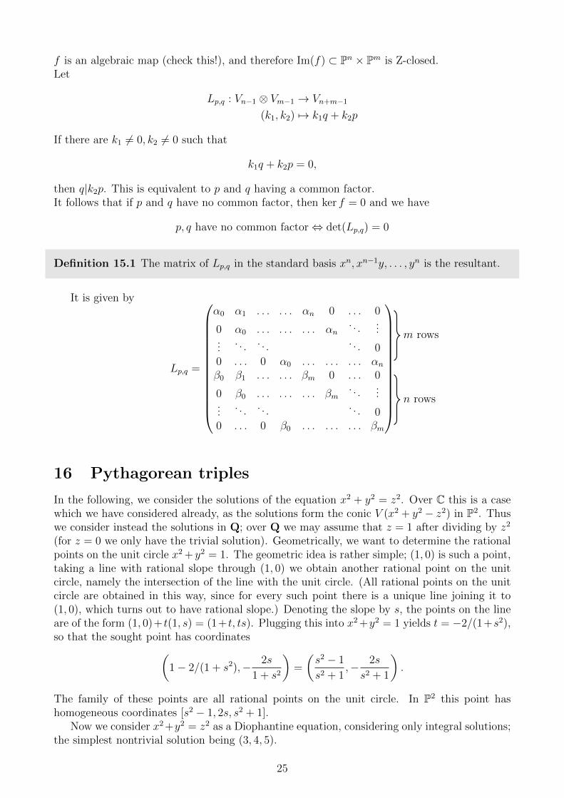
Definition 15.1 The matrix of Lp,q in the standard basis xn, xn−1y, . . . , yn is the resultant.

It is given by

Lp,q =

α0 α1 . . . . . . αn 0 . . . 0

0 α0 . . . . . . . . . αn. . .

......

. . . . . . . . . 00 . . . 0 α0 . . . . . . . . . αnβ0 β1 . . . . . . βm 0 . . . 0

0 β0 . . . . . . . . . βm. . .

......

. . . . . . . . . 00 . . . 0 β0 . . . . . . . . . βm

m rows

n rows

16 Pythagorean triples

In the following, we consider the solutions of the equation x2 + y2 = z2. Over C this is a casewhich we have considered already, as the solutions form the conic V (x2 + y2 − z2) in P2. Thuswe consider instead the solutions in Q; over Q we may assume that z = 1 after dividing by z2

(for z = 0 we only have the trivial solution). Geometrically, we want to determine the rationalpoints on the unit circle x2 + y2 = 1. The geometric idea is rather simple; (1, 0) is such a point,taking a line with rational slope through (1, 0) we obtain another rational point on the unitcircle, namely the intersection of the line with the unit circle. (All rational points on the unitcircle are obtained in this way, since for every such point there is a unique line joining it to(1, 0), which turns out to have rational slope.) Denoting the slope by s, the points on the lineare of the form (1, 0)+ t(1, s) = (1+ t, ts). Plugging this into x2 +y2 = 1 yields t = −2/(1+s2),so that the sought point has coordinates(

1− 2/(1 + s2),− 2s

1 + s2

)=

(s2 − 1

s2 + 1,− 2s

s2 + 1

).

The family of these points are all rational points on the unit circle. In P2 this point hashomogeneous coordinates [s2 − 1, 2s, s2 + 1].

Now we consider x2 +y2 = z2 as a Diophantine equation, considering only integral solutions;the simplest nontrivial solution being (3, 4, 5).

25

17 The Riemann-Hurwitz formula

Let X and Y be surfaces of genus g and h, respectively. Furthermore let f be a branchedcovering map of degree d (i.e. every non-ramification point in X has exactly d preimages) whichis ramified in only finitely many points. We denote these points by b1, . . . , bR and assume thatat reach ramification only two sheets come together.

Theorem 17.1 (Riemann-Hurwitz formula)

2− 2g = d(2− 2h)−R (7)

Proof. (sketch) We choose a triangulation of X such that b1, . . . , bR are corners of triangles. Thepreimage of this triangulation is (homeomorphic to) a triangulation of Y. Observe furthermorethat all faces and edges have exactly d preimages under f . This also holds true for all verticesexcept the b1, . . . , br which have d− 1 preimages each. Therefore, we have

χ(Y ) = dχ(X)−R (8)

It is also known that χ(X) = 2− 2h and likewise χ(Y ) = 2− 2g, giving

2− 2g = d(2− 2h)−R (9)

This can be generalized for ramifications of arbitrary multiplicity. R is then equal to thesum of all multiplicities (greater than 1) minus the number of ramifications.

We can use the Riemann-Hurwitz formula to calculate the genus of varietiesExample 17.2 Let F be a homogeneous polynomial in three variables. If F ([0, 0, 1]) 6= 0,we can canonically project V (F ) onto P1 using the projection map π([x, y, z]) := [x, y]. π isa branched covering of degree d because for fixed x and y, F (x, y, z) is a polynomial in z ofdegree d. We also know that the genus of P1 is 0, giving h = 0. However, it is hard in generalto determine the number and multiplicities of the ramifications and therefore R.

18 Points in projective space

Let V = {p1, . . . , pr} ⊂ P2.

Proposition 18.1 V can be cut out by degree r polynomials.

Proof. LetS = {F |F = L1 . . . Lr, where Li is a line through pi}

The polyomials in S all have degree r. We have that V ⊂ Z(S). Let q ∈ P2 \ V . Then there aline through every point in V that misses q. Therefore q /∈ Z(S). ⇒ V = Z(S).

Example 18.2 A set of r distinct points in P2 cannot necessarily be cut out by polyomialsof degree r − 1. For example let L ⊂ P2 be a line and let p1, . . . , pr be distinct points on theline. Let F be a polynomial of degree r − 1 which vanishes on p1, . . . , pr. Then F vanisheseverywhere on L.

26

Definition 18.3 The points p1, . . . , pk ∈ Pn are in general linear position if correspondingvectors v1, . . . , vk ∈ Cn+1 are as linearly independent as possible. This means that for eachsubset S with |S| ≤ n+ 1, dim spanS = |S|.

Proposition 18.4 Let

φ : P1 → Pd

[s, t] 7→ [sd, sd−1t, . . . , td]

be the d-Veronese. Let {p0, . . . , pd} ⊂ P1 be d+ 1 distinct points. Then {φ(p0), . . . , φ(pd)} arein general linear position.

Proof. See exercise 3 on sheet 4.

Definition 18.5 Let P0, . . . , Pn be a basis of the homogeneous polynomials of degree n. Thenthe map

P1 → Pn

[s, t] 7→ [P0(s, t), . . . , Pn(s, t)]

is called a rational normal curve.

Example 18.6 The Veronese map from P1 is an example of a rational normal curve.

Theorem 18.7 Let p1, . . . , pn+3 ∈ Pn be in general linear position. Then there is a uniquerational normal curve in Pn passing through these points.

Proof. Choose a basis of Cn+1 such that

p1 = [1, 0, . . . , 0]

p2 = [0, 1, . . . , 0]

...

pn+1 = [0, 0, . . . , 1].

We have pn+2 = [α0, . . . , αn]. We have ∀i ∈ {0, . . . , n} : αi 6= 0, because else the points wouldnot be in general linear position. We can rescale the basis vectors such that

pn+2 = [1, 1, . . . , 1].

We have pn+3 = [λ0, . . . , λn], where ∀i ∈ {0, . . . , n} : λi 6= 0 and i 6= j ⇒ λi 6= λj, because ofthe general linear position.We are looking for a rational normal curve φ : P1 → Pn and points ξ1, . . . , ξn+3 ∈ P1 such thatφ(ξi) = pi. Denote for i ∈ {1, . . . , n+ 1} : ξi = [1, ξi].Now φ(ξi) = [P1(ξi), . . . , Pn+1(ξi)] = [0, . . . , 0, 1, 0, . . . , 0] implies that (setting x = t/s) (x−ξi) |Pk for k 6= i and therefore

Pi = αi∏j 6=i

(x− ξj)

27

From φ([0, 1]) = [1, . . . , 1] we can infer that all αi are equal (we can set them equal to 1). Wehave

φ([1, 0]) = [∏i 6=1

ξi, . . . ,∏i 6=n+1

ξi] =

[1

ξ1

, . . . ,1

ξn+1

]= [λ1, . . . , λn+1]

and therefore we fix ξi = 1λi

which is possible, because λi 6= 0.

19 Rational functions.

20 Tangent Spaces I

In Differential Geometry, tangent spaces, at least for smooth submanifolds, arise very naturally.The tangent space at a single point is best described as the collection of possible startingdirections one can take when travelling from that point along the manifold. We want todevelop a similar notion for algebraic varieties. For this, we will start with the definition foraffine varieties and build from that towards a more general formulation.Let X ⊂ Cn be an affine algebraic variety, p ∈ X

Definition 20.1 (First definition of Tangent Space)

1. We define Tp(Cn) to be the complex n-dimensional vector space generated by the abstractbasis ∂1, . . . , ∂n.

2. For f ∈ C[X1, . . . , Xn], v =∑n

i=1 vi∂i ∈ Tp, let

(Dvf)p :=n∑i=1

vi∂if

∂xi(p)

3. Tp(X) := {v ∈ Tp(Cn) | ∀f ∈ I : (Dvf)p = 0}is the tangent space of X at the point p.

Note that for (Dvf)p the usual properties of differentiation, such as linearity and the Leibnizrule, hold. We will also write Dvf if there is no ambiguity concerning the basepoint.

Lemma 20.2 Let f1, . . . , fk be generators of I(X). Then

Tp(X) = {v ∈ Tp(Cn) | For i = 1, . . . , k : (Dvfi)p = 0}

Proof. Let v ∈ Tp(Cn) s.t. Dvf1 = . . . = Dvfk = 0.Then for g = h1f1 + . . .+ hkfk ∈ I(X) we have

(Dvg)p = (Dv

n∑i=1

hifi)p =n∑i=1

(Dvhi)pfi(p) + hi(p)(Dv(fi))p = 0

As, for any i, by assumption Dvfi = 0 and by definition of I(X): fi(p) = 0. So v ∈ Tp(X).This proves one inclusion. The other one is obvious.

28

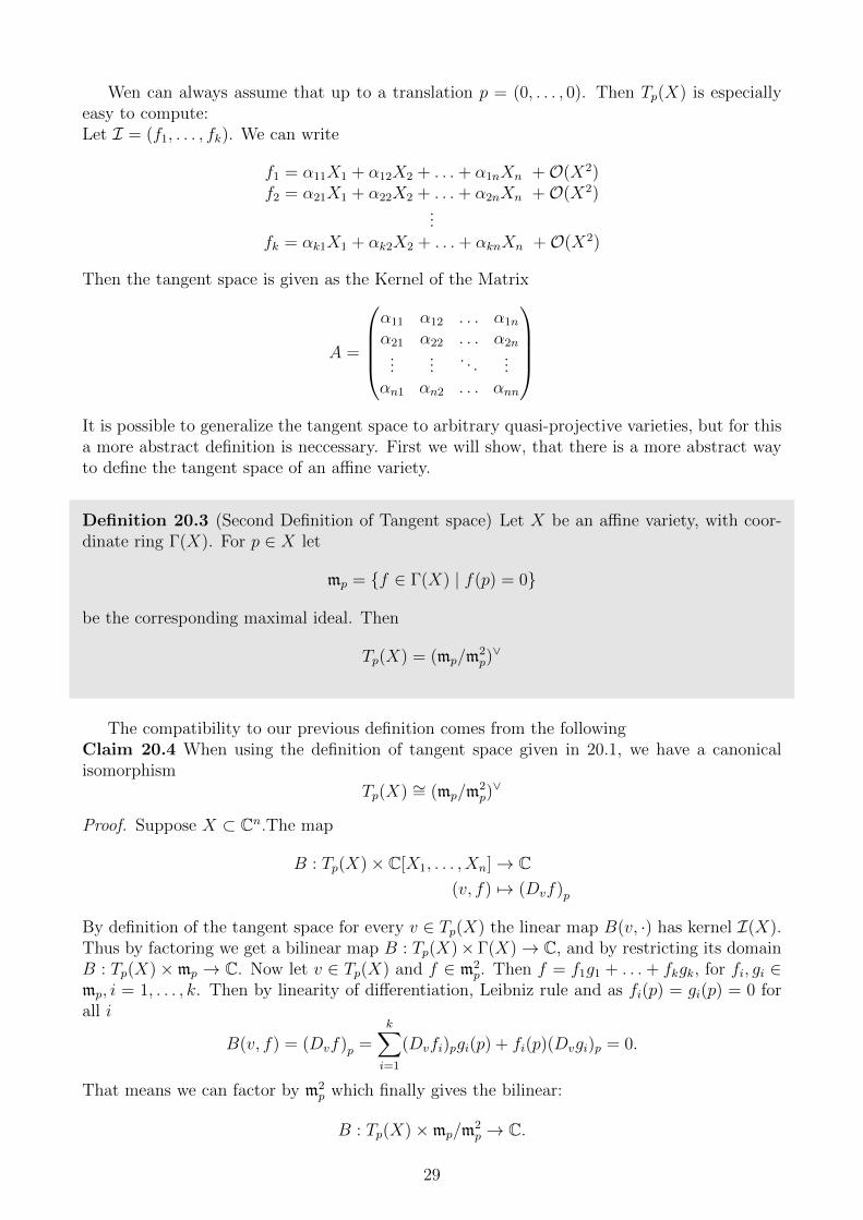
Wen can always assume that up to a translation p = (0, . . . , 0). Then Tp(X) is especiallyeasy to compute:Let I = (f1, . . . , fk). We can write

f1 = α11X1 + α12X2 + . . .+ α1nXn +O(X2)f2 = α21X1 + α22X2 + . . .+ α2nXn +O(X2)

...fk = αk1X1 + αk2X2 + . . .+ αknXn +O(X2)

Then the tangent space is given as the Kernel of the Matrix

A =

α11 α12 . . . α1n

α21 α22 . . . α2n...

.... . .

...αn1 αn2 . . . αnn

It is possible to generalize the tangent space to arbitrary quasi-projective varieties, but for thisa more abstract definition is neccessary. First we will show, that there is a more abstract wayto define the tangent space of an affine variety.

Definition 20.3 (Second Definition of Tangent space) Let X be an affine variety, with coor-dinate ring Γ(X). For p ∈ X let

mp = {f ∈ Γ(X) | f(p) = 0}

be the corresponding maximal ideal. Then

Tp(X) = (mp/m2p)∨

The compatibility to our previous definition comes from the followingClaim 20.4 When using the definition of tangent space given in 20.1, we have a canonicalisomorphism

Tp(X) ∼= (mp/m2p)∨

Proof. Suppose X ⊂ Cn.The map

B : Tp(X)× C[X1, . . . , Xn]→ C(v, f) 7→ (Dvf)p

By definition of the tangent space for every v ∈ Tp(X) the linear map B(v, ·) has kernel I(X).Thus by factoring we get a bilinear map B : Tp(X)× Γ(X)→ C, and by restricting its domainB : Tp(X)×mp → C. Now let v ∈ Tp(X) and f ∈ m2

p. Then f = f1g1 + . . .+ fkgk, for fi, gi ∈mp, i = 1, . . . , k. Then by linearity of differentiation, Leibniz rule and as fi(p) = gi(p) = 0 forall i

B(v, f) = (Dvf)p =k∑i=1

(Dvfi)pgi(p) + fi(p)(Dvgi)p = 0.

That means we can factor by m2p which finally gives the bilinear:

B : Tp(X)×mp/m2p → C.

29

This datum is equivalent to the linear map

L : Tp(X)→(mp/m

2p

)∨v 7→ (f 7→ (Dvf)p)

which we will now prove to be an isomorphism. Write p = (ξ1, . . . , ξn) such that mp = (X1 −ξ1, . . . , Xn − ξn). Assume v ∈ Tp(X) such that for all f ∈ mp (Dvf)p = 0. Then in particular

vi = (Dv(X i − ξi))p = 0,

so v = 0. This proves injectivity. Now assume ψ : mp/m2p → C is linear. Any f ∈ I(X) fulfills

f(p) = 0 and hence can be written as

f =n∑i=1

(Xi − ξi)ai + (higher terms).

As the image of f in Γ(X) is zero, ψ(f) = 0. At the same time (X i−ξi)1≤i≤k span the C-vectorspace mp/m

2p, and we have,

ψ(f) = ψ(n∑i=1

(X i − ξi)ai) =n∑i=1

ψ(X i − ξi)ai.

Let vi = ψ(X i − ξi) and

v =n∑i=0

vi∂i.

Then by what we have shown it follows that v ∈ Tp(X) and that L(v) = ψ. This provessurjectivity of L.

We now want to generalize this definition in a straightforward way to arbitrary quasi-projective varieties. One possibility would be to choose for each point an affine open neighbor-hood and apply the second definition. However, we will use a more invariant definition, whichclearly does not depend on a choice. The main problem is how to find the appropriate ringand maximal ideal so that we can do the same as in Def. 20.3. The solution comes with thefollowing

Definition 20.5 For any quasi-projective variety X and p ∈ X, we define the ring of germs ofalgebraic functions of X at p as

Op := {(U, f) | p ∈ U ⊂ X is open, f is an algebraic function on U.}/ ∼

Where the equivalence relation ∼ is defined as:

(U, f) ∼ (V, g)⇔ ∃W ⊂ U ∩ V : W open and f |W = g|W

It is an easy exercise that together with the induced addition and multiplication, this isindeed a local ring where the maximal ideal consists of the classes of functions that vanish atp.

30

Definition 20.6 (Third and last definition of the Tangent space) Let X be any quasi-projectivevariety and p ∈ X. Let Op be the ring of germs of algebraic functions at p, mp its maximalideal. Then the tangent space of X at p is

Tp(X) :=(mp/m

2p

)∨.

Again, we will show that this is compatible with our previous definitions:Claim 20.7 Let X is a quasi-projective variety, p ∈ X. Let Tp(X) be the Tangent space at pas in Def. 20.6. If V ⊂ X is an affine open subset and p ∈ V , there is a canonic isomorphismbetween Tp(V ) as in Def. 20.3 and Tp(X).

Proof.We will use the following commutative algebra lemma which you can check for yourself:

Lemma 20.8 Let R be ring and m ⊂ R a maximal ideal. Any R/m vector space M isisomorphic as an R-module to its localization: M ∼= M ⊗R Rm

As restriction to an open neighborhood does not change the ring of functions, we can assumethat X = V . Let A = Γ(V ) be the ring of functions of the affine variety V and mp the maximalideal belonging to p. By exercise sheet 8, Ex. 2, we know that Op ∼= Amp . Let mp the image ofmp in OK . Now we consider the exact sequence of A-modules:

0→ m2p → mp → mp/m

2p → 0.

Localization at mp gives:

0→ m2p ⊗ Amp → mp → mp/m

2p ⊗ Amp → 0

Now you should note that m2p ⊗ Amp = m2

p and use the lemma to get:

mp/m2p∼= mp/m

2p.

Taking the dual on both sides yields the isomorphism of the tangent spaces.

21 Tangent Space II

22 Blow-up

As a motivation for the blowup construction, consider the polar coordinates

ρ : R× [0, π]/ ∼ −→ R2, ρ : (r, φ) 7→ (r cos(φ), r sin(φ)),

where (r, 0) ∼ (−r, π). Note that the domain is a bit unusual, but on U = {r 6= 0}, ρ isisomorphic to the classical polar coordinates defined on R>0 × S1.

Note the characteristic feature of ρ: It is an isomorphism on U = {r 6= 0} and contracts thecircle r = 0 onto the zero-point. Polar coordinates are used to simplify calculations in calculus.We consider an analog construction in algebraic geometry, the blowup.

31

The blowup of A2 at 0 is defined by

Bl0A2 = {(x, y), [u, v] ∈ A2 × P1 | xv − yu = 0}

together with the natural mapρ : Bl0A2 −→ A2

given by projection on the first factor. It is easy to see that ρ is an isomorphism on Bl0 A2 \{ρ−1(0, 0)}, while it contracts the central fiber ρ−1(0, 0) ∼= P1 to the point (0, 0).

In fact, when considering the blowup construction over the real numbers R, we obtain themotivating example above (up to an isomorphism; use RP1 = S1/± 1 = [0, π]/ ∼).

Then further discussion of the blowup, see Harris, Shafarevich, Hartshorne. Explicit com-putations are given in the solutions to sheet 9.

23 Dimension I

Topic is the equivalence of the definitions and several things about transcendence degree.Christoph recommended hungerford’s algebra for more details.

24 Dimension II

25 Sheaves

Let X be a topological space. A presheaf of abelian groups (or rings, etc.) on X is a contravari-ant functor F from the poset category of open subsets of X to the category of abelian groups(rings, etc.). It is standard to denote F (U) by Γ(U,F ) (whose elements are called sections ofF over U), and, for V ⊂ U , to denote the image of s ∈ F (U) under F (U)→ F (V ) by s|V .

Roughly speaking, a sheaf is a presheaf whose sections are determined locally, and compati-ble sections can be patched together; it establishes relations between local and global propertiesof a space. Formally, a sheaf on X is a presheaf F on X such that for every open subset Uof X and every open covering {Ui} of U the following hold: (i) if s ∈ F (U) and s|Ui

= 0 forall i then s = 0; (ii) if {si} is a family of sections si ∈ F (Ui) with si|Ui∩Uj

= sj|Ui∩Ujfor every

i, j then there is a section s ∈ F (U) such that s|Ui= si for all i. (By (i) the section s must be

unique.) Another way of putting this (giving a clue of how to generalize to sheaves with valuesin less concrete categories): we have an equalizer diagram

F (U)→∏

F (Ui) ⇒∏

F (Ui ∩ Uj)

were the first map is given by s 7→ {s|Ui} and the the other maps are {si} 7→ {si|Ui∩Uj

} and{si} 7→ {sj|Ui∩Uj

}. (Sometimes, for instance in analysis books, a different definition of sheavesis used, involving the espace etale.)

Let F be a presheaf on X. Notice that if x ∈ X is a point, the set of open neighborhoodsU of x is directed under reverse inclusion; this gives a direct system F (U) (where the maps arethe restrictions). The stalk of F at x, denoted Fx, is the direct limit lim−→F (U) of this directsystem. The construction (using the disjoint union, see exercise sheet 3 of the commutativealgebra course) used to demonstrate the existence of the direct limit shows that we may thinkof Fx as having as elements equivalence classes [(s, U)] with U an open neighborhood of x ands ∈ F (U) (germs of sections of F at x); [(s, U)] and [(t, V )] are considered as equal if thereis an open neighborhood W ⊂ U ∩ V of x with s|W = t|W . If U is an open neighborhood ofx, the canonical map F (U) → Fx belonging to the direct limit is by taking the germ at x,

32

s 7→ [(s, U)]; these maps induce a map F (U) →∏

x∈U Fx which is injective whenever F is asheaf.Example 25.1 If X is a variety (topological space, C∞-manifold), then we have (in the obviousway) a sheaf of regular (continuous, C∞-) functions on X. The reason that this is a sheaf isthat the notion of a regular (continuous, differentiable) function is defined locally.

Example 25.2 The constant sheaf associated to an abelian group, the skyscraper sheaf.

Example 25.3 Let X and Y be spaces, U an open subset of X. A sheaf F on X induces oneon U , denoted F |U . If f : X → Y is a continuous map, the direct image sheaf f∗F of F isthe sheaf on Y given by the composite of F and the functor from the category of open subsetsof Y to the category of open subsets of X by taking the preimage under f .

A morphism of (pre-)sheaves is simply a functorial morphism. Every morphism φ : F → Gof presheaves on X gives naturally rise to notions such as its kernel, cokernel, image, and so on(see exercise sheet 11); also it induces (by the functoriality of lim−→, noticing that every morphismof presheaves gives a morphism of direct systems) for every x ∈ X a map φx : Fx → Gx ofstalks (which is explicitly given by φx([(s, U)]) = [(φU(s), U)]). A sequence F → G → H ofpresheaves on X is exact iff F (U)→ G (U)→H (U) is exact for all open subsets U of X.

However, the presheaf cokernel of a morphism of sheaves need not be a sheaf (but thepresheaf kernel is one); this leads to sheafificiation (see exercise sheet 11). A sequence F →G →H of sheaves on X is exact iff it is exact at all stalks.Example 25.4 The sequence of sheaves of abelian groups on C

0→ 2πiZ→ OholC

exp−−→ Ohol,∗C → 0

is exact since it is exact at stalks (every nowhere vanishing holomorphic function is locally theexponential of some holomorphic function). The sequence of sections need, however, not beexact: for

0→ 2πiZ→ OholC (C∗) exp−−→ Ohol,∗

C (C∗)→ 0

cannot be exact as exp : OholC (C∗) → Ohol,∗

C (C∗) is not surjective (idC∗ is not in the image, asthere is no global logarithm on C∗).

26 Schemes I

Motivation for schemes: capturing nilpotents (varieties ignore nilpotents, e.g. V (x) = V (x2),the rings of algebraic functions are reduced); algebraic geometry over ground fields that arenot algebraically closed, such as finite fields (the word on the street is that algebraic geometryover finite fields comes up in number theory, apparently this leads to some kind of unificationof geometry and arithmetic).

A ringed space is a pair (X,OX) consisting of a space X and a sheaf of rings OX on X; OX issaid to be the structure sheaf of X. A morphism of ringed spaces is a pair (f, f ]) : (X,OX)→(Y,OY ) consisting of a continuous map f : X → Y and a morphism f ] : OY → f∗OX ofsheaves on Y . A locally ringed space is a ringed space such that all stalks of the structuresheaf are local rings. A morphism of locally ringed spaces is a morphism of ringed spaces(f, f ]) : (X,OX) → (Y,OY ) such that for every x ∈ X the canonical map f ]x : OY,f(x) → OX,xexplicitly given by f ]x([(s, U)]) = [(f ]U(s), f−1(U))] is a local homomorphism.Example 26.1 If X is a space, then (X,Ocont

X ) is a locally ringed space, since OcontX,x is a local

ring for every x (the maximal ideal being the germs of functions vanishing at x). Similiarly for(X,Osm

X ), X denoting a C∞-manifold. In fact a C∞-manifold of dimension n can be viewed asa locally R-ringed second-countable Hausdorff topological space which is locally isomorphic (asa locally R-ringed space) to (Rn,Osm

Rn).

33

Let A be a ring, consider the topological space Spec A; its definition and some of itstopological properties were mentioned in the exercises of the commutative algebra course. Mostnotably Spec A ≈ Spec Ared, so that the topology on Spec A is insensitive to nilpotents; thisis captured by the structure sheaf. The definition of the structure sheaf of Spec A is describedin Hartshorne.

An affine scheme is a locally ringed space that is isomorphic to Spec A for some ring A. Ascheme is a locally ringed space (X,OX) which admits an open covering {Ui} such that every(Ui,OX |Ui) is an affine scheme.Example 26.2 The affine scheme Cn is defined to be Spec C[x1, . . . , xn].

27 Schemes II

Here he just proved Prop. 2.2. and Prop. 2.3. in Hartshorne. The main point is that theproperties established in Prop. 2.2. are nice to have (in the lecture the definition of thestructure sheaf of Spec A was motivated by these properties), and that Prop. 2.3. comes as agreat relief since it is much easier to think about the (less-structured) category of rings thanthe highly-structured category of affine schemes. (Here a comparision with the fairly involveddefinition of a C∞-manifold was drawn.)

34