Lecture Notes for Mathematics 601Error Correcting Codes and Algebraic Curves

Patrick J. Morandi

Fall 2001

1

Contents

1 Introduction to Coding Theory 31.1 Introduction to the Course . . . . . . . . . . . . . . . . . . . . . . . . . . . . 31.2 Definition of Error Correcting Codes . . . . . . . . . . . . . . . . . . . . . . 31.3 Parameters of a Code . . . . . . . . . . . . . . . . . . . . . . . . . . . . . . . 51.4 Linear Codes . . . . . . . . . . . . . . . . . . . . . . . . . . . . . . . . . . . 51.5 Error Correction . . . . . . . . . . . . . . . . . . . . . . . . . . . . . . . . . 81.6 Bounds on Codes . . . . . . . . . . . . . . . . . . . . . . . . . . . . . . . . . 101.7 Cyclic Codes . . . . . . . . . . . . . . . . . . . . . . . . . . . . . . . . . . . 12

2 Introduction to Algebraic Geometry 152.1 Affine Curves . . . . . . . . . . . . . . . . . . . . . . . . . . . . . . . . . . . 152.2 Projective Varieties . . . . . . . . . . . . . . . . . . . . . . . . . . . . . . . . 162.3 The Function Field of a Curve . . . . . . . . . . . . . . . . . . . . . . . . . . 182.4 Nonsingular Curves . . . . . . . . . . . . . . . . . . . . . . . . . . . . . . . . 212.5 Curves over non-Algebraically Closed Fields . . . . . . . . . . . . . . . . . . 23

3 Algebraic Function Fields and Discrete Valuation Rings 253.1 Discrete Valuation Rings . . . . . . . . . . . . . . . . . . . . . . . . . . . . . 263.2 Discrete Valuation Rings of k(x)/k . . . . . . . . . . . . . . . . . . . . . . . 313.3 Discrete Valuation Rings of F/k . . . . . . . . . . . . . . . . . . . . . . . . . 32

4 Divisors and the Riemann-Roch Theorem 354.1 Divisors of a Function Field . . . . . . . . . . . . . . . . . . . . . . . . . . . 354.2 The Riemann-Roch Theorem . . . . . . . . . . . . . . . . . . . . . . . . . . . 434.3 Fields of Genus 0 and 1 . . . . . . . . . . . . . . . . . . . . . . . . . . . . . 45

5 Goppa Codes 485.1 Goppa Codes coming from Fq(x)/Fq . . . . . . . . . . . . . . . . . . . . . . . 50

6 Examples of Function Fields 546.1 The Connection Between Points and Places . . . . . . . . . . . . . . . . . . 546.2 Connections Between Divisors . . . . . . . . . . . . . . . . . . . . . . . . . . 556.3 Elliptic Curves . . . . . . . . . . . . . . . . . . . . . . . . . . . . . . . . . . 566.4 Hermitian Curves . . . . . . . . . . . . . . . . . . . . . . . . . . . . . . . . . 60

7 The Hasse-Weil Theorem 647.1 The Riemann Zeta Function . . . . . . . . . . . . . . . . . . . . . . . . . . . 647.2 Riemann Zeta Functions of Number Fields . . . . . . . . . . . . . . . . . . . 657.3 Riemann Zeta Functions of Curves . . . . . . . . . . . . . . . . . . . . . . . 66

2

1 Introduction to Coding Theory

1.1 Introduction to the Course

This course will discuss error correcting codes and connections with algebraic geometry.When coding theory began in the 1940s, the main mathematical technique was linear algebra.Later, ring theory was used, notably the theory of polynomial rings and quotient rings. Inthe 1970s, Goppa discovered a method for producing codes from algebraic curves, and hisclass of curves gave some nice theoretical results in the theory of error correcting codes.After spending some time on the basics of coding theory, we will develop the theory ofalgebraic curves and algebraic function fields in order to define Goppa codes and prove someresults about their error correction capability. This will require spending some time on thebasics of algebraic geometry, allowing non-algebraically closed base fields. However, sincewe will concentrate on curves, we will be able to bypass much of the difficult machinery ofalgebraic geometry. In fact, it is possible to work purely field theoretically, as does the bookof Stichtenoth. However, I believe that this is too narrow a viewpoint, and that thinkinggeometrically gives better insight.

One aspect where Goppa codes are beneficial is in finding asymptotic bounds on codes.Without describing what this means, it is necessary to be able to produce long codes. Oneof the most important class of codes, BCH codes, can produce long codes but at the expenseof requiring the use of increasingly large finite fields. Goppa codes, which can be viewed asa generalization of BCH codes, get around this problem.

Finding long Goppa codes reduces the problem of finding algebraic curves with manyrational points. We will see that, for any algebraic curve over a finite field, there is ananalogue of the Riemann Zeta function. (There is also such an analogue for every algebraicnumber field.) The Riemann hypothesis, which states that the Riemann Zeta’s nontrivialzeros lie on the line Re(s) = 1

2 , and which remains unproven, was proved by Andre Weil forthe Zeta functions associated to curves over a finite field. We shall see how this fact leadsto a bound on the number of rational points of a curve, and what implications this has forcoding theory.

There is a website for this course. The URL is math.nmsu.edu/∼pmorandi/math601.

1.2 Definition of Error Correcting Codes

Let F be a finite field and let F n be the collection of all n-tuples over F . This is an n-dimensional F -vector space. A code over F is a (nonempty) subset of F n. It does not haveto be a subspace although all of our examples will be subspaces. We will sometimes writeelements of F n as strings of elements without using commas or parentheses. The elementsof a code are called codewords, and the elements of F n are called words.

Before we give some notation, we will follow the normal practice of writing Fq for theunique, up to isomorphism, field with q elements.

3

Example 1.1. Let F = F2. Then 0, 1 is a code in F and 00, 11 is a code in F 2. Likewise,000, 111 is a code in F 3 and 00000, 11111 is a code in F 5.

Example 1.2. Let

H =

0 0 0 1 1 1 10 1 1 0 0 1 11 0 1 0 1 0 1

.

Then the kernel of H is a code in F 7. This is called the Hamming code, and was the first realexample of an error correcting code. We will investigate this code further in a little while.

The important property of a code is its ability to correct errors. Let us discuss this ideastarting with an example. In 1979 the Mariner 9 spacecraft took black and white pictures ofMars. These pictures were created by using 64 shades of grey. Each pixel of a photographwas assigned a shade of grey. Each picture consisted of a 600 by 600 grid of pixels. Thus,to transmit one photograph, the spacecraft had to send 360,000 pieces of data, each piecerepresenting the color of a pixel. Suppose that the shades of grey were represented by anumber from 1 to 64 in binary. Thus, we could represent any color with a string of sixbinary digits. If, in transmission, an error was made, then NASA would incorrectly color thecorresponding pixel. Since electromagnetic activity can easily cause such errors, this wouldbe a problem. NASA wanted an encoding system that would take received data, performsome sort of test, and determine if the received data was the same as that send, and, if not,determine what was the actual transmitted data. What they did was to encode each coloras a string of 32 binary digits. Of the 232 possible strings, 64 of them were valid codewords.

Suppose that a codeword is transmitted, but errors are made. One can recognize thatan error is made if one sees that the received word is not a codeword. The main principleof error detection, Maximum Likelihood Detection (MLD) assumes that few errors are morelikely than many errors. Therefore, the codeword that differs from the received word in thefewest number of components is the most likely transmitted codeword. All error correctingschemes use this principle. For example, with the code 000, 111, if 101 is received, thenMLD would assume that 111 was transmitted. However, with 00, 11, if 01 or 10 wastransmitted, then MLD would not distinguish between 00 and 11. Even worse, with thecode 0, 1, if a codeword is transmitted but an error is made, the error cannot be detectedbecause all elements of F are codewords.

To make more precise the notion of closeness of words, we define a metric on F n. Thefunction d : F n × F n → Z defined by d(u, v) is equal to the number of components in whichu and v vary. In other words, if xi is the i-th component of a vector x, then

d(u, v) = |i : ui 6= vi| .

The function d is in fact a metric. To see this, note that the property d(u, v) ≥ 0 andd(u, v) = 0 if and only if u = v is clear. Similarly, d(u, v) = d(v, u) is clear. The triangleinequality is not hard, but is not completely obvious. We need to show that if u, v, w ∈ F n,

4

then d(u,w) ≤ d(u, v) + d(v, w). Then

d(u,w) = |i : ui 6= wi| .

We note that i : ui 6= wi is a subset of i : ui 6= vi ∪ i : vi 6= wi since if ui = vi andvi = wi, then ui = wi. Thus,

d(u,w) = |i : ui 6= wi| ≤ |i : ui 6= vi ∪ i : vi 6= wi|≤ |i : ui 6= vi|+ |i : vi 6= wi| = d(u, v) + d(v, w).

This metric will play a quiet but important role in coding theory.

1.3 Parameters of a Code

There are some important parameters attached to a code C over F = Fq. The first, calledthe length of the code, is the value of n for which C is a subset of F n. The next, which wewill label k, is defined as

k = logq(|C|).

If C is a subspace of F n, then k = dimF (C), and so k is the dimension of the code. To definethe final parameter, we need some preliminary concepts. The third invariant is labeled dand is the distance of the code C. It is defined as

d := min d(u, v) : u 6= v ∈ C .

It should not be a problem that we are using d both for the metric and for the distance of acode. These three parameters are then positive integers. The parameters, in order n, k, d,of the codes of the first example are (2, 1, 2), (3, 1, 2), and (5, 1, 5), respectively. With a littlecalculation, we see that the parameters of the Hamming code are (7, 4, 3). Occasionally wewill refer to a code with parameters n, k, and d as an (n, k, d)-code.

1.4 Linear Codes

A code that is a subspace of F n is said to be a linear code. All of the codes we will considerin this course will be linear codes. We will view the elements of F n as row matrices. Thereare some useful matrices attached to a linear code C ⊆ F n. The first is called a generatormatrix. It is a matrix G whose rows form a basis for C. This is an k×n matrix, and its rowspace is equal to C. The code C is then given, in terms of G, by

C =

vG : v ∈ F k .

The second matrix is called a parity check matrix. This is a matrix H of full rank for whichC is the right nullspace of HT . That is, u ∈ C if and only if uHT = 0. Alternatively, u ∈ C

5

if HuT = 0. Thus, by rethinking about codewords as column matrices, C is the nullspace ofH. It is then an (n− k)× n matrix. Moreover, GHT = 0 since xGHT = 0 for all x ∈ F k.

To see the symmetry of these matrices, we first give some notation. We will use · forthe “usual dot product” on F n; that is, u · v =

∑

i uivi. This is no longer an inner productsince u · u = 0 can occur with u 6= 0, for instance, if F = F2 and u has an even number ofcomponents equal to 1. In terms of matrix multiplication, u · v = uvT . Mimicking what isdone for inner product spaces, we define the dual code C⊥ of a code C by

C⊥ = u ∈ F : u · v = 0 for all v ∈ C .

We claim that H is a generator matrix for C⊥ and G is a parity check matrix for C⊥. Toprove this, we first note the following matrix properties: if A is an r × s matrix, then (i) ifAx = 0 for all x ∈ F s, then A = 0, and (ii) if yA = 0 for all y ∈ F r, then A = 0. Theseare both straightforward to prove. As for the claim, first note that the row space of H iscontained in C⊥. For, if x ∈ F n−k, then xH · v = (xH)vT = x(vHT )T = x · 0 = 0 forall v ∈ C. This implies that dim(C⊥) ≥ n − k = n − dim(C). However, if u ∈ C⊥, then0 = u · xG = u(xG)T = uGT xT for all x ∈ F k. Therefore, uGT = 0, and so C⊥ is containedin the right nullspace of G. Because G has rank k and is a k × n matrix, its nullspace hasdimension n− k. Thus, dim(C⊥) ≤ n− k, and so both inequalities yield dim(C⊥) = n− k.Furthermore, this equality shows that the row space of H is C⊥ and that C⊥ is the rightnullspace of G. This finishes the proof of the claim.

Example 1.3. Let C be the Hamming code. Then C has parity check matrix H, as definedearlier. A simple calculation shows that 1110000, 0101010, 1001100, 1101001 form a basisfor C. Thus, we may take

G =

1 1 1 0 0 0 00 1 0 1 0 1 01 0 0 1 1 0 01 1 0 1 0 0 1

as a generator matrix for C. The code C⊥ is then the nullspace of G, which has basis0111100, 1101001, 1011010. Thus,

C⊥ = 0000000, 0111100, 1101001, 1011010, 1010101, 1100110, 0001111 .

Having a linear code allows us to give an alternative description of the distance of a code.First of all, we define the weight of a word to be w(u) = d(u, 0), the number of nonzerocomponents of u. Then since d(u, v) = w(u− v), we see that

d = min w(x) : x ∈ C, x 6= 0 .

By listing out the elements of the Hamming code, it is easy to see that the smallest weight

6

of a codeword is 3. For the dual code to the Hamming code, the listing of its elements showsthat C⊥ has distance 4.

Example 1.4. The extended Golay code, discovered by Golay, the codiscoverer of the Ham-ming code, has generator matrix

G =

1 0 0 0 0 0 0 0 0 0 0 0 0 1 1 1 1 1 1 1 1 1 1 10 1 0 0 0 0 0 0 0 0 0 0 1 1 1 0 1 1 1 0 0 0 1 00 0 1 0 0 0 0 0 0 0 0 0 1 1 0 1 1 1 0 0 0 1 0 10 0 0 1 0 0 0 0 0 0 0 0 1 0 1 1 1 0 0 0 1 0 1 10 0 0 0 1 0 0 0 0 0 0 0 1 1 1 1 0 0 0 1 0 1 1 00 0 0 0 0 1 0 0 0 0 0 0 1 1 1 0 0 0 1 0 1 1 0 10 0 0 0 0 0 1 0 0 0 0 0 1 1 0 0 0 1 0 1 1 0 1 10 0 0 0 0 0 0 1 0 0 0 0 1 0 0 0 1 0 1 1 0 1 1 10 0 0 0 0 0 0 0 1 0 0 0 1 0 0 1 0 1 1 0 1 1 1 00 0 0 0 0 0 0 0 0 1 0 0 1 0 1 0 1 1 0 1 1 1 0 00 0 0 0 0 0 0 0 0 0 1 0 1 1 0 1 1 0 1 1 1 0 0 00 0 0 0 0 0 0 0 0 0 0 1 1 0 1 1 0 1 1 1 0 0 0 1

.

This is a 12× 24 matrix. It can be viewed in the form [B | A] with A and B both 12× 12matrices. In fact, G = [I12 | A], where

A =

0 1 1 1 1 1 1 1 1 1 1 11 1 1 0 1 1 1 0 0 0 1 01 1 0 1 1 1 0 0 0 1 0 11 0 1 1 1 0 0 0 1 0 1 11 1 1 1 0 0 0 1 0 1 1 01 1 1 0 0 0 1 0 1 1 0 11 1 0 0 0 1 0 1 1 0 1 11 0 0 0 1 0 1 1 0 1 1 11 0 0 1 0 1 1 0 1 1 1 01 0 1 0 1 1 0 1 1 1 0 01 1 0 1 1 0 1 1 1 0 0 01 0 1 1 0 1 1 1 0 0 0 1

.

The Golay code is the code C, where C is the row space of G. The matrix G has rank 12, sothe code has dimension 12. Thus, there are 212 = 4096 codewords. This code has distance8, which can be verified in a hopelessly tedious manner by calculating the weight of all 4095nonzero codewords, or by proving some facts, by induction, about the rows of G. One seesthat the distance is at most 8 since the last row has weight exactly 8.

The Voyager spacecrafts visited Jupiter, Saturn, Uranus, and Neptune, taking pictures ofeach planet and their moons. The following picture was taken by Voyager 2. The photographs

7

taken by these spacecrafts utilized the Golay code to encode the data representing thepictures. A photograph consists of a rectangular grid, and at each grid point, or pixel,a color is given. For the Voyager spacecrafts, the use of the Golay code allowed the photosto be made with up to 4096 colors. Each color was represented as a codeword in the Golaycode. To send the information representing one picture, each pixel was described by thecodeword representing the color of that pixel. This codeword was a 24-tuple of binary digits.Since the Golay code has distance 8, it can correct up to three errors. Thus, each codewordtransmitted could have up to three errors without losing any data.

1.5 Error Correction

We make formal the meaning of an error correcting code, and we shall shortly see theconnection between the distance and the error correction capabilities of the code.

Definition 1.5. A code C is s-error detecting if whenever at least one but at most s errorsare made in any codeword, then the resulting word is not a codeword.

From this definition and that of the distance of a code, it is clear that a code of distanced can detect up to d−1 errors. A more important definition for us is that of error correcting.

Definition 1.6. A code C is said to be t-error correcting if a word is a distance at most tfrom some codeword, then its distance from every other codeword is greater than t.

To help to understand this definition, suppose that a codeword v is transmitted andat most t errors are made, meaning at most t components of the codeword are changed,resulting in a word w. If the code is t-error correcting, then since w is a distance of at mostt from v, then the distance from w to any other codeword is greater than t. Therefore, vis the closest codeword to w. Using MLD, we would correct w to v, and thus recover thecorrect codeword.

Example 1.7. The code 0, 1 cannot correct any errors, nor can 00, 11. However,000, 111 can correct 1 error. If 111 is transmitted but one error is made, the resulthas distance 2 from 000. The same is true starting with 000. The code 00000, 11111 cancorrect two errors.

Example 1.8. The Hamming code can correct one error. Moreover, there is a nice decodingalgorithm, if F = F2. Suppose that v is a codeword, and one error is made in transmittingv, resulting in a word w. Then w = v + ei, where ei is the i-th standard basis vector ofF 7. Multiplying by the Hamming matrix H, we get Hw = H(v + ei) = Hv + Hei = Hei.Now, an easy calculation shows that Hei is the i-th column of H. Therefore, if we identifywhich column of H is Hw, then we will determine i. Once we know i, we can recover v asv = w + ei. This example illustrates an aspect of coding theory; we would like codes thatcan correct errors and for which there is an efficient decoding algorithm.

8

We know show the relation between the distance and the error correction capability of acode.

Theorem 1.9. Suppose that a code C has distance d. Then C is t-error correcting fort = b(d− 1)/2c but is not (t + 1)-error correcting.

Proof. We give a metric-theoretic proof of this fact. Let t = b(d− 1)/2c. Suppose that w isa word a distance at most t from v. We need to prove that w is a distance greater than tfrom any other codeword. Suppose that u is another codeword. If d(w, u) ≤ t, then considerthe closed disks of radius t centered at v and u, respectively. Then w is in both disks. Bythe triangle inequality, we have

d(v, u) ≤ d(v, u) + d(u,w) ≤ 2t < d,

a contradiction to the definition of d. Therefore, d(w, u) > t, so the code is indeed t-error correcting. To see that C is not (t + 1)-error correcting, let u, v be codewords withd(u, v) = d. Note that d = 2t + 1 or d = 2t + 2, depending on whether d is odd or even.If we change t + 1 of the components of u that differ from those of v to make them equalto the corresponding components of v, then we obtain a word w with d(u, w) = t + 1 butd(w, v) = d(u, v) − (t + 1) = d − (t + 1) ≤ t + 1. This shows that C is not (t + 1)-errorcorrecting.

From this theorem it is clear that the Hamming code is 1-error correcting since its distanceis 3.

If we have a linear code C with parity check matrix H, we can use cosets to help decode.Given a word w, the syndrome of w is Hw. Therefore, the syndrome is 0 exactly when theword is a codeword. The possible syndromes are in 1-1 correspondence with the cosets ofC, since C + u = C + w if and only if Hu = Hw. If a codeword v is incorrectly transmittedas w, then e = w − v is the error word. We have He = Hw, so e and w have the samesyndrome. Since C + w = C + e, we look in the coset C + w for the smallest weight vector;this is our error word e by MLD. To use this coset decoding, we need a list of syndromesand corresponding smallest weight error vectors. These vectors are called coset leaders. Forexample, the following table would be the coset decoding table for the Hamming code.

Syndrome Coset Leader000 0000000001 1000000010 0100000011 0010000100 0001000101 0000100110 0000010111 0000001

9

The Maple worksheet cosets.mws, available on the class website, will produce this table.

1.6 Bounds on Codes

Suppose you have to transmit two pieces of information. You could use the code 0, 1,but that would give you no error correction. You could use 000, 111 to be able to correctone error, or up to 1

3 of the digits. You could use 00000, 11111 and correct up to twoerrors, or 2

5 of the digits. In general, by making the strings longer, we can have better errorcorrection. However, longer codewords mean more effort in sending, receiving, and decoding.So, we would like to have codes as short as possible with as good error correction as possible.What restrictions are there? Are there any relationships between the parameters n, k, andd? There are several relationships, all that give upper bounds or lower bounds for d. Tostate some of these bounds, we set Aq(n, d) to be the largest size of a code of length n anddistance d. Much of coding theory has been to determine the values of this function and indetermining the asymptotic behavior of Aq(n, d) as a function of δ = d/n as n →∞.

To help in some of the proofs, we first give a counting argument. Consider the sphere ofradius r centered at a word v. To pick a word a distance i from v, we need to change i ofthe components of i; there are

(ni

)

choices for these components. Each component can bechanged in q − 1 ways since |F | = q. Therefore, there are

(ni

)

(q − 1)i total words a distanceof i from v. Therefore, the sphere contains a total of

∑ri=0

(ni

)

(q − 1)i words.There are many bounds on codes, although we restrict our attention to just three. The

first bound gives a lower bound of the size of a code with given parameters n and d. Mostbounds give upper bounds.

Proposition 1.10 (Gilbert-Varshamov Bound).

Aq(n, d) ≥ qn

∑d−1i=0

(ni

)

(q − 1)i.

Proof. Let C be a code of maximal size of length n and distance d. The spheres of radiusd− 1 centered at codewords then cover the entire space of words, since if there is a word adistance of at least d from every codeword, then we could add it to C without changing nor d. If M is the size of this code, then from our calculation of the size of spheres, we haveM ·

∑d−1i=0

(ni

)

(q − 1)i ≥ qn, which yields the bound.

This bound says that there exists a code of length n and distance d, and with M elements,such that M ≥ qn/

(

∑d−1i=0

(ni

)

(q − 1)i)

. It does not say anything about arbitrary codes.

Proposition 1.11 (Singleton Bound). Let C be a code with parameters n, k, and d. Thend ≤ n− k + 1. Therefore, Aq(n, d) ≤ qn−d+1.

Proof. Consider the function ϕ : C → F n−d+1 given by ϕ(x1, . . . , xn) = (x1, . . . , xn−d+1). Inother words, ϕ removes the last d − 1 components of a codeword. Since every codeword of

10

C has weight at least d, the function ϕ is 1-1. Consequently, |C| ≤∣

∣F n−d+1∣

∣. Since this istrue for any code of length n and distance d, we have Aq(n, d) ≤

∣

∣F n−d+1∣

∣ = qn−d+1. Takinglogarithms to the base q, we get k ≤ n− d + 1, or d ≤ n− k + 1.

If a code C satisfies d = n− k + 1, then the code is said to be an MDS code (maximumdistance separable).

The following bound is also called the sphere packing bound.

Proposition 1.12 (Hamming Bound). If t = b(d− 1)/2c, then

Aq(n, d) ≤ qn

∑ti=0

(ni

)

(q − 1)i.

Proof. Suppose that we have a code with length n and distance d, and for which it has Mcodewords. Let v be a codeword, and consider the sphere of radius t centered at v. As wehave seen this sphere contains

∑ti=0

(ni

)

(q − 1)i words. Since the code can correct t errors,the spheres of radius t centered at codewords are disjoint. Therefore, since there are qn totalwords,

qn ≤ Mt

∑

i=0

(

ni

)

(q − 1)i,

orM ≤ qn

∑ti=0

(ni

)

(q − 1)i.

Since this is true for any such code, we get the Hamming bound.These last two codes give an upper bound, in terms of n and d, of the number of elements

of any code with length n and distance d.

The codes Goppa constructed from algebraic curves yield a better asymptotic lower boundthan the Gilbert-Varshamov bound. By asymptotic bounds, we mean the investigation of

lim supn→∞

logq(Aq(n, d))n

.

The reason for considering asymptotic bounds comes from Shannon’s channel coding theo-rem. If we define the information rate of a code to be k/n, then the theorem says that givenany ε > 0, there is a code with information rate at least R for which the probability of in-correct decoding of a received word is less than ε. However, in order to make the probabilityof incorrect decoding low with a fixed k/n, then n must be large. This theorem is not statedquite correctly; there is a limit on how large the information rate can be; this limit is calledthe capacity of the channel. A description of this can be found in Roman’s book.

11

1.7 Cyclic Codes

To define some of the important classes of codes, we first define cyclic codes. First of all, letσ : F n → F n be the shift map; that is, σ(x1, . . . , xn) = (xn, x1, x2, . . . , xn−1). A code C issaid to be cyclic provided that σ(C) = C. To give an alternate description of cyclic codes,first consider the F -algebra of polynomials F [x]. We may view F n as a subspace of F [x] viathe map ϕ : (a0, . . . , an−1) 7→ a0 + a1x + · · ·+ an−1xn−1. Then F n is mapped isomorphicallyonto the subspace of polynomials of degree less than n. We can interpret σ with respect tothis embedding. Since σ(a0, . . . , an−1) = (an−1, a0, . . . , an−2), we have

ϕ (σ(a0, . . . , an−2)) = an−1 + a0x + · · ·+ an−2xn−1 = an−1 + x(a0 + · · ·+ an−2xn−2)

≡ x(a0 + · · ·+ an−2xn−2 + an−1xn−1) mod(xn − 1).

Because of this, if we view F n ∼= F [x]/(xn − 1), then σ corresponds to multiplication by x.Therefore, a code C ⊆ F [x]/(xn − 1) is cyclic if and only if xC = C. Since C is already anF -vector space, this additional condition is equivalent to that C be an ideal of F [x]/(xn−1).Now, since F [x] is a PID, every ideal of F [x]/(xn − 1) is principal and is generated by adivisor of xn − 1. Thus, cyclic codes of length n are in 1-1 correspondence with divisors ofxn − 1.

Suppose that xn−1 factors as xn−1 = g(x)h(x). Consider the code C = (g(x))/(xn−1);that is, C is the code consisting of all polynomial cosets that are multiples of g(x). Ifg(x) = g0 + g1x + · · · + xn−k, then

g(x), xg(x), . . . , xk−1g(x)

is a basis for C, where

f(x) = f(x)+(xn−1). Therefore, k = n−deg(g(x)). We call g(x) the generator polynomialof the code.

Let K be a finite extension field of F . If α1, . . . , αt ∈ K, let fi(x) be the minimalpolynomial over F of αi, and let g(x) be the least common multiple of the fi(x). Then g(x)is the monic polynomial of least degree for which each αi is a root. We then can use g(x) tobuild a cyclic code of length n, where n is any integer for which g(x) divides xn − 1. Thiscode then consists of all polynomial cosets p(x) for which p(αi) = 0 for all i. Note that forg(x) to divide xn − 1, we need each αi to be a root of xn − 1; that is, we need αn

i = 1.Recall from the theory of finite fields, the multiplicative group of any finite field is cyclic.

A generator of the multiplicative group F ∗ is called a primitive element of F . If α is aprimitive element of Fn+1, then all powers of α are roots of xn − 1, and we can use powersof alpha to build a code of length n. Note that n + 1 must be a power of a prime for Fn+1

to exist.

Example 1.13. With a rearrangement of its digits, the Hamming code is an example ofa cyclic code. To see this, let α be a primitive root of F8. Since we may view F8 asF8 = F2[x]/(x3 + x + 1), we can view its elements as 3-tuples over F2. The nonzero elements1, α, . . . , α6 of F8 then correspond to the columns of the Hamming matrix H. By reorderingthe columns if necessary, we view H = (1, α, . . . , α6), where we think of these elements as

12

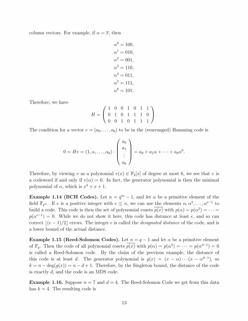
column vectors. For example, if α = x, then

α0 = 100,

α1 = 010,

α2 = 001,

α3 = 110,

α4 = 011,

α5 = 111,

α6 = 101.

Therefore, we have

H =

1 0 0 1 0 1 10 1 0 1 1 1 00 0 1 0 1 1 1

.

The condition for a vector v = (a0, . . . , a6) to be in the (rearranged) Hamming code is

0 = Hv = (1, α, . . . , α6) ·

a0

a1...a6

= a0 + a1α + · · ·+ a6α6.

Therefore, by viewing v as a polynomial v(x) ∈ F2[x] of degree at most 6, we see that v isa codeword if and only if v(α) = 0. In fact, the generator polynomial is then the minimalpolynomial of α, which is x3 + x + 1.

Example 1.14 (BCH Codes). Let n = qm − 1, and let α be a primitive element of thefield Fqm . If e is a positive integer with e ≤ n, we can use the elements α, α2, . . . , αe−1 tobuild a code. This code is then the set of polynomial cosets p(x) with p(α) = p(α2) = · · · =p(αe−1) = 0. While we do not show it here, this code has distance at least e, and so cancorrect b(e− 1)/2c errors. The integer e is called the designated distance of the code, and isa lower bound of the actual distance.

Example 1.15 (Reed-Solomon Codes). Let n = q − 1 and let α be a primitive elementof Fq. Then the code of all polynomial cosets p(x) with p(α) = p(α2) = · · · = p(αd−1) = 0is called a Reed-Solomon code. By the claim of the previous example, the distance ofthis code is at least d. The generator polynomial is g(x) = (x − α) · · · (x − αd−1), sok = n− deg(g(x)) = n− d + 1. Therefore, by the Singleton bound, the distance of the codeis exactly d, and the code is an MDS code.

Example 1.16. Suppose n = 7 and d = 4. The Reed-Solomon Code we get from this datahas k = 4. The resulting code is

13

We now consider some specific examples of BCH codes.

Example 1.17. Consider F16 = F2[x]/(x4 +x+1), the splitting field over F2 of x4 +x+1. Ashort calculation shows that any root α of x4+x+1 is a primitive element of F16. To see this,recall that since F∗16 has order 15, Lagrange’s theorem implies that α is a primitive elementprovided that α3 6= 1 and α5 6= 1. Since the minimal polynomial of α is x4 + x + 1, whichdoes not divide x3−1 or x5−1, neither of these polynomials has α as a root. We consider theBCH code of all polynomials cosets having α, α2, . . . , α6 as roots. Then n = 15. To calculatek, we calculate the generator polynomial g(x). This is the least common multiple of theminimal polynomials of the six roots. The minimal polynomial of α and α2 is x4 + x + 1.The minimal polynomial of α3 and α6 is x4 + x3 + x2 + x + 1 and the minimal polynomialof α5 is x2 + x + 1. One way to find these is to note that every element of F16 is a root ofx16 − x. If you factor this into irreducible polynomials, you need to check which irreduciblehas a given αi as a root. Alternatively, you can find the generator polynomial by using theMaple worksheet generator.mws, which is available on the course website. In any case, weget g(x) = x10 + x8 + x5 + x4 + x2 + x + 1. This has degree 10, so k = n − deg(g(x)) = 5.This code can correct three errors since the designated distance is 7.

Example 1.18. Consider the code built from the same field F16 but with designated distance5. Then the code comes from the roots α, α2, α3, α4. In this case, the generator polynomialis x8 + x7 + x6 + x4 + 1, and so n = 15 and k = 15 − 8 = 7. By lowering the designateddistance, we have increased the dimension of the code.

14

2 Introduction to Algebraic Geometry

While the error correcting codes defined by Goppa can be described purely in terms of fields,they are better understood by also viewing them geometrically. We will discuss the basicconcepts of algebraic geometry and see how the study of (nonsingular projective) algebraiccurves is equivalent to the study of algebraic function fields in one variable. Furthermore,by thinking of fields, we will help to justify why we need to discuss projective curves insteadof restricting only to affine curves. A brief treatment of the concepts of algebraic geometryneeded for coding theory can be found in the book Codes and Curves, by Walker.

To do algebraic geometry we need to use algebraically closed fields. Recall that a field k isalgebraically closed if every nonconstant polynomial in k[x] has a root in k. The fundamentaltheorem of algebra states that C is algebraically closed. Neither R nor Q is algebraicallyclosed as x2 + 1 has no root in either field. Nor is any finite field F algebraically closed, forif F = a1, . . . , an, then (x− a1) · · · (x− an) + 1 has no root in F . If F is an arbitrary field,then it has an algebraic extension that is algebraically closed; this field is called an algebraicclosure of F . Such a field is unique up to isomorphism.

2.1 Affine Curves

Let k be an algebraically closed field. We denote the polynomial ring over k in 2 variables byk[x, y]. Algebraic geometry studies solutions to polynomial equations. We define the affineplace A2(k) to be the set k2 of all pairs over k. If it is not important to keep track of thefield k, we will write A2 in place of A2(k). If P = (a, b) ∈ A2 and f ∈ k[x, y], we will denoteby f(P ) the evaluation of f at P . If f ∈ k[x, y], then the affine curve f = 0 is defined to be

Z(f) =

P ∈ A2 : f(P ) = 0

.

This set is sometimes called the zero set of f .

Example 2.1. The curve y = x2 in A2 is a parabola. In general, a conic section is thezero set of a polynomial of degree 2. For instance, x2 + y2 = 1 is a circle and xy = 1 is ahyperbola. The curve y2 = x3 is sometimes called a cuspidal cubic curve.

Example 2.2. An elliptic curve is a curve given by an equation y2 = f(x), where f(x) is acubic polynomial with no repeated roots. For example, y2 = x3 − x is an elliptic curve.

Example 2.3. A hyperelliptic curve is a curve given by an equation y2 = f(x), where f(x)is a polynomial of degree at least 4 and with no repeated roots. For example, y2 = x5 − 1 isan elliptic curve over C, or over any algebraically closed field of characteristic not 5.

Example 2.4. Suppose that k = R, a field that is not algebraically closed. There are nosolutions to the equation x2 + y2 + 1 = 0 over R, so Z(x2 + y2 + 1) is empty. However,if k = C, then there are solutions, including (i, 0). It is to have solutions to polynomial

15

equations that the base field is assumed to be algebraically closed. If f(x, y) is a polynomialover an algebraically closed field k, and if b ∈ k, then f(x, b) is a polynomial in the onevariable x. If f(x, b) is not constant, then it has roots in k, and so f(x, y) = 0 has solutionsin A2(k).

If X is an algebraic curve over k, then the ideal of X is

I(X) = f ∈ k[x, y] : f(P ) = 0 for all P ∈ X .

If f(x, y) = p(x, y)e1 · · · pn(x, y)en is the factorization of a polynomial f into irreduciblefactors, then it is easy to see that I(Z(f)) = (p1 · · · pn). Moreover, the coordinate ring of Xis the quotient ring Γ(X) = k[x, y]/I(X). One way of thinking about the coordinate ring isto consider it the ring of polynomial functions on X. For, two polynomials f and g inducethe same function X → k precisely when f − g ∈ I(X), which is equivalent to the cosets fand g being equal.

A topological space is said to be irreducible if it cannot be written as the union of twoproper subcurves. If f = gh, then Z(f) = Z(g) ∪ Z(h). From this, if f is a squarefreepolynomial, it follows that Z(f) is irreducible if and only if f is irreducible. Alternatively,X is irreducible if and only if Γ(X) is an integral domain.

2.2 Projective Varieties

For students who have studied topology, the construction of projective varieties parallelsthat of constructing the real projective plane. We define an equivalence relation ∼ onA3 \ (0, 0, 0) by defining that (a, b, c) ∼ (a′, b′, c′) if there is a nonzero scalar λ witha′ = λa, b′ = λb, and c′ = λc. Geometrically, the equivalence class of a point is the linethrough the origin that passes through the point. We will write (a : b : c) for the equivalenceclass of (a, b, c), and P2 will denote the set of all equivalence classes. This is the projectiveplane. Note that (a : b : c) represents a point in the projective plane only if at least one ofthe coordinates is nonzero.

Note that polynomial functions are not well defined on points of projective space. How-ever, we can get around this problem. A polynomial f ∈ k[x, y, z] is said to be homogeneousif every monomial of f has the same degree. Alternatively, f is homogeneous if there is aninteger m with f(λx, λy, λz) = λmf(x, y, z) for all λ ∈ k. If f is homogeneous and P ∈ P2,then the equation f(P ) = 0 is well defined; in other words, if P ∼ Q, then f(P ) = 0 ifand only if f(Q) = 0. Therefore, we can define zero sets of collections of homogeneouspolynomials. If f is a homogeneous polynomial, then the projective curve f = 0 is the zeroset

Z(f) = P ∈ Pn : f(P ) = 0 .

We define a projective curve to be irreducible in exactly the same way as for affine curves;if f is a squarefree homogeneous polynomial, then it follows that Z(f) is irreducible if and

16

only if f is irreducible.We can define a coordinate ring for projective curves. If X is a projective curve, then

I(X) is defined to be

I(X) = 〈f ∈ k[x, y, z] : f is homogeneous and f(P ) = 0 for all P ∈ X〉 .

The homogeneous coordinate ring S(X) is the quotient ring k[x, y, z]/I(X). As with affinecurves, a projective curve is irreducible if and only if its ideal is a prime ideal, and thishappens exactly when S(X) is an integral domain.

Example 2.5. Consider the projective parabola X given by yz = x2. If (a : b : c) ∈ X, thenbc = a2. If c 6= 0, then by dividing by c, we may assume that c = 1. Then, (a, b) is on theaffine parabola y = x2. On the other hand, if c = 0, then a = 0, and b 6= 0 for (a : b : c) tobe a valid point. Then, by dividing by b, we have the point (0 : 1 : 0). Thus, we can thinkof X as the union of the affine parabola y = x2 and the extra point (0 : 1 : 0). Note thatthe affine parabola is obtained by setting z = 1 in the equation yz = x2. Moreover, there isanother affine parabola inside X, and this other curve contains (0 : 1 : 0). If we set y = 1,then we have the equation z = x2, which again represents a parabola. The point (0 : 1 : 0)is a point of this affine parabola. The purpose of considering this second affine parabola isthat any point of X is a point on some affine curve in X.

Example 2.6. Let X be the projective elliptic curve y2z = x3 − xz2. The affine ellipticcurve y2 = x3 − x is an affine curve in X; we can map it into X via (a, b) 7→ (a : b : 1). Theimage is X − (0 : 1 : 0); if (a : b : c) ∈ X and c = 0, then the equation y2z = x3 − xz2

forces a = 0. Then b 6= 0 since (a : b : c) ∈ P2. Thus, we may divide by b to assume b = 1,and so the only point on X for which c = 0 is (0 : 1 : 0). As with the previous example, theaffine equation is obtained from the projective equation by setting z = 1.

Example 2.7. In the previous examples we started with a projective curve and found anaffine curve inside it. In this example we start with an affine curve and produce a projectivecurve. Let Y be the curve y = x3. By adding a third variable z, we can use y−x3 to get thehomogeneous polynomial yz2−x3. The affine curve Y sits inside the projective curve yz2 = x3

as in the previous examples. Similarly, y2 + 1 = x4 yields the homogeneous polynomialy2z2 + z4 = x4. What we are doing is adding enough copies of z to each monomial so thateach has degree equal to the highest degree of a monomial of the original polynomial. To havea formula for doing this, if f(x, y) has degree d, then zdf(x/z, y/z) is the homogenizationof f(x, y). The resulting projective curve is called the projective closure of the affine curvef = 0. In general, if Z(f) is a projective curve, then any point of the form (a : b : 0) ofZ(f) is called a point at infinity. If g(x, y) = f(x, y, 1), then Z(f) is the union of the affinecurve g = 0 and the points of infinity. The polynomial g(x, y) is called a dehomogenizationof f(x, y, z) (at the variable z).

17

Note that if fh(x, y, z) is the homogenization of f(x, y), then f(x, y) = fh(x, y, 1). Con-versely, if g(x, y, z) is homogeneous of degree d, and if f(x, y) = g(x, y, 1), then

g(x, y, z) = zdeg(g)−deg(f)fh(x, y).

We do not, in general, recover g(x, y, z) by homogenizing g(x, y, 1) since this polynomial mayhave smaller degree than the degree of g(x, y, z). For example, if g(x, y, z) = z2 + xz + yz,then g(x, y, 1) = 1 + x + y has degree 1 while g(x, y, z) has degree 2.

2.3 The Function Field of a Curve

Suppose that an affine curve X is irreducible. Then its coordinate ring Γ(X) is an integraldomain, and so has a quotient field, which we denote by k(X). This is the field

k(X) = g/h : g, h ∈ Γ(X), h 6= 0 .

Let x and y be the images of x and y in Γ(X). The definition of Γ(X) shows that Γ(X) =k[x, y]. That is, Γ(X) is generated as a k-algebra by x and y. The field k(X) then containsthe field k(x, y) generated by x and y. Since the quotient field of an integral domain is thesmallest field containing the domain, we see that k(X) = k(x, y). Therefore, k(X) is thefield extension of k generated by two elements u, v, and subject to the relation f(u, v) = 0.

To give other another view of the function field, suppose that X is the zero set of theirreducible polynomial f(x, y). If we define an equivalence relation ∼ on the ring

S = g(x, y)/h(x, y) : g, h ∈ k[x, y], h /∈ (f)

by g/h ∼ g′/h′ if gh′ − g′h ∈ (f) ⊆ k[x, y], then k(X) ∼= S/ ∼. To verify this interpretation,note that an arbitrary element of k(X) is of the form g/h with g, h ∈ k[x, y], where wecontinue to write bars to represent the image of a polynomial in Γ(X). When are g/h andg′/h′ equal in k(X)? Since k(X) is the quotient field of Γ(X), this occurs exactly whengh′ = g′h. Finally, this occurs when gh′ − g′h = 0, or gh′ − g′h ∈ (f).

We may define a topology on a curve by defining a set to be open if it is empty, or if itscomplement is finite. Thus, proper closed sets are finite. This is a special example of theZariski topology on an algebraic variety; curves are special examples of varieties. We willview k(X) as the field of rational functions defined an open subset of the curve X; a rationalfunction is simply a function that can be represented as a quotient of polynomials.

Example 2.8. The function field of the affine parabola y = x2 is the quotient field ofk[x, y]/(y − x2). This ring is isomorphic to k[t], the rational function field in one variable t;they are isomorphic via the map that sends t to x + (y − x2). Therefore, the function fieldis isomorphic to k(t).

Example 2.9. The coordinate ring of the curve X = Z(y2−x3) is k[x, y]/(y2−x3). This ring

18

is isomorphic to k[t2, t3], a subring of k[t]. These rings are isomorphic via the map x 7→ t2

and y 7→ t3. The function field of this curve is then the quotient field of k[t2, t3], which isk(t). Note that y/x represents a rational function on X as does x2/y. Furthermore, thesefunctions agree since y/x = x2/y in k(X). Therefore, a rational function can be representedin more than one way as a quotient of polynomials.

Example 2.10. The coordinate ring of the elliptic curve y2 = x3−x is k[x, y]/(y2−x3−x).We claim that its function field is isomorphic to k(t)

(√t3 − t

)

. To see this, note that thecoordinate ring is k[x, y], and so its function field is k(x, y). That is, the function field isgenerated as an extension field of k by x and y. Now, we have y2 = x3 − x. Therefore y isalgebraic over k(x), and so k(x, y) = k(x)(y) ∼= k(x)

(√x3 − x

)

. The element x cannot bealgebraic over k, so k(x) ∼= k(t), the rational function field in t.

Let f(x, y, z) be an irreducible homogeneous polynomial, and let X = Z(f). We can alsodefine a function field of X. Let ∼ be the equivalence relation on the set

g(x, y, z)/h(x, y, z) : g, h ∈ k[x, y, z] are homogeneous of the same degree, h /∈ (f) ∪ 0

given by g/h ∼ g′/h′ if and only if gh′ − g′h ∈ (f). The function field k(X) is then the setof equivalence classes, under the natural operations.

Note that any f/g ∈ k(X) determines a well defined function on an open subset of X: ifg, h are both homogeneous of degree d, then if λ is nonzero, then

g(λa, λb, λc)h(λa, λb, λc)

=λdg(a, b, c)λdh(a, b, c)

=g(a, b, c)h(a, b, c)

.

The function g/h is defined for all points P except when h(P ) = 0. We may then think ofk(X) in much the same way as we think of the function field of an affine curve.

We now show that the function field of a projective curve can be calculated by findingthe function field of an affine curve.

Proposition 2.11. Let f(x, y, z) be an irreducible homogeneous polynomial. Let X = Z(f)be a projective curve and if U is the affine curve Z(f(x, y, 1)), then k(X) ∼= k(U).

Proof. We will define a ring homomorphism ϕ : Γ(U) → k(X) and show that ϕ is injective.Thus, ϕ induces a homomorphism k(U) → k(X), which necessarily is injective. We will thenbe done by showing that this map is surjective. To define ϕ, write g(x, y) = f(x, y, 1). Forh(x, y) ∈ k[x, y], define ϕ(h) = h(x/z, y/z). Note that if deg(h) = d, then h(x/z, y/z) =hh(x, y, z)/zd, and this represents an element of k(X). This map is well defined, since ifh′ − h ∈ (g), then h′ = h + gl for some l ∈ k[x, y]. Then h′(x/z, y/z) = h(x/z, y/z) +g(x/z, y/z)l(x/z, y/z). By our hypothesis on f , we have g(x/z, y/z) = f(x, y, z)/zdeg(f).Therefore, g(x/z, y/z)l(x/z, y/z) = 0 in k(X) by the definition of k(X). Thus, ϕ(h) =ϕ(h′); this proves that ϕ is well defined. It is a simple exercise to see that ϕ is a ring

19

homomorphism. To prove injectivity, suppose that ϕ(h) = 0. Then h(x/z, y/z) = 0 ink(X). Note that h(x/z, y/z) = hh(x, y, z)/zdeg(h). For this to be zero in k(X), we havehh(x, y, z) = f(x, y, z)m(x, y, z) for some m. Dehomogenizing, we get

h(x, y, z) = hh(x, y, 1) = f(x, y, 1)m(x, y, 1)

= g(x, y)m(x, y, 1).

Therefore, h = 0. Thus, ϕ is injective. For surjectivity, every element of k(X) is rep-resented by a quotient h(x, y, z)/l(x, y, z) of homogeneous polynomials of the same de-gree. Let their common degree be d. Then h(x, y, z)/l(x, y, z) = zdh(x, y, 1)/zdl(x, y, 1) =h(x, y, 1)/l(x, y, 1). This represents an element of k(U), and this element maps via ϕ toh(x, y, z)/l(x, y, z). Therefore, ϕ is surjective, and so k(U) ∼= k(Z).

Example 2.12. Let X be the projective parabola yz = x2. The affine parabola Y =Z(y − x2) is obtained from dehomogenizing yz − x2. Therefore, k(X) = k(Y ) ∼= k(t).Similarly, the function field of yz2 = x3 is k(t), and the function field of the projectiveelliptic curve y2z = x3 − xz2 is k(t)

(√t3 − t

)

.

There are important subrings of the function field of a curve. First, if X is a projectiveor affine curve, then

k[X] = ϕ ∈ k(X) : ϕ is defined at every point of X .

This is called the ring of regular functions on X, and is the ring of globally defined rationalfunctions on X. If X is affine, then one can show that k[X] ∼= Γ(X), but that if X isprojective, then k[X] = k. Next, let P ∈ X. Then the local ring of X at P is the set

OP (X) = ϕ ∈ k(X) : ϕ is defined at P .

This is the ring of regular functions defined locally at P . For ϕ(P ) to be defined, ϕ must bedefined in an open neighborhood of P , since if ϕ = g/h, then P /∈ Z(h), and so ϕ is definedon the open neighborhood h 6= 0 of P . For convenience, we will typically write OP in placeof OP (X). It is a local ring; its unique maximal ideal is

MP = ϕ ∈ OP : ϕ(P ) = 0 .

A short exercise shows that MP is an ideal of OP . Furthermore, if ϕ ∈ OP \MP , then wemay write ϕ = f/g with f(P ) 6= 0. Then g/f ∈ OP is an inverse for ϕ. Therefore, sinceevery element outside MP is a unit, MP is the unique maximal ideal of OP . If Y = Z(f) isan affine curve, then OP (Y ) =

g/h ∈ k(Y ) : h(P ) 6= 0

.

Proposition 2.13. Let P be a point of an irreducible affine curve X = Z(f), and letmP = g ∈ k[X] : g(P ) = 0. Then OP = k[X]mP .

20

Proof. By definition, k[X] ⊆ OP . Moreover, everything in k[X] \mP is invertible in OP , sok[X]mP ⊆ OP . Conversely, let ϕ ∈ OP . Then we may write ϕ = g/h with g, h ∈ k[X], bythe definition of k(X). Since ϕ is defined at P , we have h(P ) 6= 0. Therefore, h /∈ mP , sog/h ∈ k[X]mP . Thus, OP = k[X]mP .

It is not hard to show that if P = (a, b), then mP is generated by the images in k[X] ofthe polynomials x− a and y − b.

Let X = Z(f) be an irreducible projective curve, and let Y = Z(g) be the affine curveobtained by dehomogenizing f . We have seen that k(X) = k(Y ). If P ∈ Y , the definitionof local ring then shows that OP (X) = OP (Y ). Therefore, the local ring at a point can bedetermined from the previous proposition.

Example 2.14. The line X = Z(y) has function field k(t). We determine the local ringsof points on X. Let P = (a, 0) ∈ X. Note that Γ(X) = k[x, y]/(y) ∼= k[t], and k(X)is the quotient field of this ring. The isomorphism k(X) ∼= k(t) sends the image of apolynomial f(x, y) to f(t, 0). We claim that OP (X) = k[t](t−a), the localization of k[t] atthe maximal ideal (t − a). For, g(x, y)/h(x, y) ∈ OP (X) if h(a, 0) 6= 0. Therefore, h(t, 0) isnot divisible by t − a, and so g(t, 0)/h(t, 0) ∈ k[t](t−a). The reverse inclusion is easy sinceg(t, 0)/h(t, 0) ∈ k[t](t−a) is defined at P since t− a does not divide h(t, 0).

2.4 Nonsingular Curves

To have a complete correspondence between function fields and projective curves, we mustrestrict to nonsingular curves. Suppose that f(x, y, z) is a homogeneous polynomial. Itdefines a projective curve X in P2, and we refer to it as a plane curve. By recalling formulasfor tangent lines from calculus, we say that the curve X is nonsingular at a point P ∈ X ifat least one of the three partial derivatives ∂f/∂x, ∂f/∂y, or ∂f/∂z do not vanish at P . IfX is nonsingular at every point P , then we say that X is a nonsingular curve. Similarly, anaffine curve g = 0 is nonsingular at a point P if ∂g/∂x and ∂g/∂y do not both vanish at P ,and the curve itself is nonsingular if it is nonsingular at all its points.

Example 2.15. The affine parabola y = x2 is nonsingular, for the partial derivatives ofy−x2 are −2x and 1; neither vanish simultaneously. Similarly, Z(y−x3) and Z(x2 + y2−1)are nonsingular. However, Z(y2 − x3) is singular at the origin.

Example 2.16. Consider the projective parabola yz = x2. The partial derivatives are −2x,z, y; they only simultaneously vanish at (0, 0, 0), which does not represent a point in P2.Therefore, the parabola is nonsingular. However, the projective closure of the cubic curvey = x3 is X = Z(yz2 − x3). Here, the partial derivatives are −3x2, z2, 2yz, which vanishesat (0 : 1 : 0) ∈ X. Therefore, this curve has a singularity. Note that the singularity occursat the point at infinity.

21

Example 2.17. The elliptic curve X = Z(y2z−x3 +xz2) is nonsingular if the characteristicof k is not 2. To see this, the three partial derivatives of y2z − x3 + xz2 are −3x2 + z2, 2yz,and y2 + 2xz. It is easy to see that all three partials vanish only at x = y = z = 0, and sothere is no point on X for which this happens. In fact, if y2 = f(x) is any elliptic curve,where f(x) is a cubic polynomial with no repeated roots, then this curve is nonsingular. For,a point P = (a, b) on the curve satisfies b2 = f(a). The partials of y2 − f(x) are −f ′(x) and2y; for these to vanish at P , we must have b = 0 and f ′(a) = 0. Then f(a) = f ′(a) = 0, andthis cannot happen since a would then be a multiple root of f(x).

Example 2.18. Any hyperelliptic curve is nonsingular, as long as the characteristic of thebase field is not 2. The argument of the previous example works word for word to prove thata hyperelliptic curve is nonsingular.

By making use of some theorems from Math 582, we can now begin to give the connectionbetween function fields and curves. We first note that a commutative ring is said to havedimension 1 if all nonzero prime ideals are maximal. It is not an obvious result, but thecoordinate ring of an affine curve has dimension 1. Also, the local ring at a point on anycurve also has dimension 1. The general result is that the geometric dimension of an affinealgebraic variety is equal to the ring theoretic dimension of its coordinate ring, and thatthese are also equal to the transcendence degree over k of the function field k(X). Next,if X is a curve, then OP (X) is a local Noetherian domain of dimension 1 for any P ∈ X.We have already remarked that its dimension is 1. It is Noetherian because the coordinatering of an affine curve is a quotient ring of k[x, y]. The coordinate ring is then Noetherian,and since OP (X) is a localization of the coordinate ring, it is also Noetherian. We haveseen above that OP (X) is a local ring. Let A be a local domain with maximal ideal M , andset F = A/M , a field. Then A is a discrete valuation ring if and only if it is Noetherian,dimension 1, and dimF (M/M2) = 1. Note that F = k for A = OP (X); this can be seenindirectly in the proof below.

Theorem 2.19. Let X = Z(f) be an irreducible curve. Then P ∈ X is nonsingular if andonly if OP (X) is a discrete valuation ring of k(X).

Proof. By the remarks above, it is enough to prove that P is nonsingular if and only ifdimk(MP /M2

P ) = 1, where MP is the maximal ideal of OP . Let M = (x − a, y − b), amaximal ideal of k[x, y]. Define a map θ : M → k2 by

θ(g) = (∂g∂x

(P ),∂g∂y

(P )).

We note that θ yields a vector space isomorphism M/M2 ∼= k2. The polynomial f yields the1-dimensional subspace V = ((f) + M2) /M2 of M/M2, and θ(V ) has dimension 1 if andonly if P is nonsingular, and it has dimension 0 otherwise. Recall that k[X] ∼= k[x, y]/(f)

22

and OP = k[X]mp , where mP = g ∈ k[X] : g(P ) = 0 = M/(f). Then

mP /m2P = M/(f)/

(

M2 + (f)/)

(f) ∼= M/(

M2 + (f))

The maximal ideal MP of OP is then mPOP , and so MP /M2P∼= mP /m2

P by a Math 582exercise. Thus,

MP /M2P∼= mP /m2

P∼= M/((f) + M2) ∼=

(

M/M2))

/V

by one of the homomorphism theorems of vector space theory. Therefore, MP /M2P has

dimension 1 if and only if P is nonsingular.

Example 2.20. The curve X = Z(y2 − x3) is singular at the origin. The coordinate ringof X is k[t2, t3], and so the local ring at the origin is k[t2, t3](t2,t3). This is a proper subringof the discrete valuation ring k[t](t). By another characterization of discrete valuation rings,a local Noetherian domain of dimension 1 is a discrete valuation ring if and only if it isintegrally closed. The ring k[t2, t3](t2,t3) is not integrally closed since t is integral over it; tsatisfies the polynomial T 2− t2. However, t /∈ k[t2, t3](t2,t3), which shows that this ring is notintegrally closed.

2.5 Curves over non-Algebraically Closed Fields

Classical algebraic geometry uses algebraically closed fields in order to have solutions topolynomial equations. However, in several situations, including coding theory, we need towork with arbitrary fields.

Let k be an arbitrary field, and let K be an algebraically closed extension field of k.An affine curve over k is a curve Z(f) ⊆ A2(K) such that f(x, y) ∈ k[x, y]. Similarly, aprojective curve over k is a curve Z(f) ⊆ P2(K) such that f(x, y, z) ∈ k[x, y, z]. An affinecurve Z(f) over k is said to be absolutely irreducible if f(x, y) is irreducible in K[x, y]. Ananalogous definition holds for projective curves.

If X = Z(f) is an affine curve over k, then its ideal over k is

I(X/k) = I(X) ∩ k[x, y] = g(x, y) ∈ k[x, y] : g(P ) = 0 for all P ∈ X

and its k-coordinate ring isΓ(X/k) = k[x, y]/I(X/k).

This is a subring of the coordinate ring Γ(X). If X is absolutely irreducible, then thefunction field K(X) exists, we define the k-function field k(X) to be the quotient field ofΓ(X/k). Therefore, we see that k(X) is the set of all quotients of polynomials g(x, y)/h(x, y),where g/h = g′/h′ if gh′ − g′h ∈ fk[x, y]. We similarly can define the k-function field ofan irreducible projective curve. We also can define a k-version of the local ring of a point,

23

which we also denote by OP (X/k). This is the ring

OP (X/k) = ϕ ∈ k(X) : ϕ(P ) is defined= OP (X) ∩ k(X).

This notation does not show the dependence on k, but this will not give us a problem sincewe will not consider this concept for two fields at a time.

The characterization of nonsingularity in terms ofOP can be made relative to k as follows.If X is a curve over k, then P ∈ X is nonsingular if and only ifOP (X/k) is a discrete valuationring. The proof of this is a moderately standard use of facts about discrete valuation rings,and we won’t give it here.

A point P = (a, b) on a curve X is said to be a k-rational point if a, b ∈ k. We writeX(k) for the set of all k-rational points of X. Thus, X = X(K). To simplify terminology,we will often refer to a K-rational point as simply a point, and use the terminology rationalpoint to note a point whose coordinates are in k (or some other subfield of K). A curve overk is nonsingular if it is nonsingular as a curve over K. That is, X is nonsingular if everypoint P ∈ A2(K) lying on X is nonsingular.

As we will see, a major problem in working with codes coming from algebraic geometryis to find curves over Fq with lots of rational points.

Example 2.21. Let n ≥ 3 be an integer, and consider the projective curve xn + yn = zn.Fermat’s last theorem says that there are noQ-rational points of this curve having all nonzerocoordinates.

Example 2.22. The projective curve X = Z(x2 + y2 + z2) over R has no R-rational points.However, it has lots of C-rational points, such as (1 : 0 : i).

Example 2.23. The projective curve X = Z(x2 + y2) over R is not absolutely irreducibleeven though x2 + y2 is irreducible in R[x, y], since over C the polynomial x2 + y2 factors as(x + iy)(x− iy). Therefore, the k-curve Z(f) need not be absolutely irreducible even if f isirreducible over k.

Example 2.24. We will see near the end of the course that Weil’s proof of the Riemannhypothesis for curves over a finite field Fq yields a bound on the number of rational points.This bound, which is in terms of the genus g of the curve and of the size q of the base field,says that the number N of rational points satisfies the inequality

|N − (q + 1)| ≤ 2g√

q.

We will define the genus in the first chapter of Stichtenoth; the proof of this bound is donein Chapter 5. Let X be the curve over Fq2 given by xq+1 + yq+1 = 1. This is called theHermitian curve over Fq2 . It turns out that the genus of this curve is g = q(q − 1)/2, andthat N = 1 + q3, the largest possible given the bound above.

24

3 Algebraic Function Fields and Discrete ValuationRings

Let F/k be a field extension. Then F is said to be an algebraic function field in one variableover k if there is an element x ∈ F that is transcendental over k and for which [F : k(x)] < ∞.Recall that if x is transcendental over k, then the field k(x) is isomorphic to a rational functionfield in one variable over k. We will not distinguish between transcendental elements andvariables from now on. These fields are precisely the function fields of algebraic curvesdefined over k. We have indicated, without full proof, why the function field of a curve issuch a field. For the converse, if F is generated over k(x) by a single element y, then sincey is algebraic over k(x), there is an irreducible polynomial p(t) ∈ k(x)[t] for which p(y) = 0.By clearing denominators, we may view p(t) ∈ k[x][t], and the equation p(y) = 0 yields anequation f(x, y) = 0 with f a polynomial in two variables over k. Then F is the functionfield of Z(f) ⊆ A2.

We note one simple but important property of algebraic function fields in one variable,which we state as a proposition.

Proposition 3.1. Let F/k be an algebraic function field in one variable. If t ∈ F is tran-scendental over k, then [F : k(t)] < ∞.

Proof. There is an x ∈ F transcendental over k and with [F : k(x)] < ∞. We will be doneby proving that x is algebraic over k(t), since then [k(t)(x) : k(t)] < ∞, and then

[F : k(t)] = [F : k(t)(x)][k(t)(x) : k(t)]

≤ [F : k(x)][k(t)(x) : k(t)]

is finite since both terms are finite. To show that x is algebraic over k(t), we know that t isalgebraic over k(x). Therefore, there are fi(x) ∈ k(x) with tn +fn−1(x)tn−1 + · · ·+f0(x) = 0.By writing each fi(x) as a quotient of polynomials and then clearing denominators, we havean equation of the form an(x)tn + an−1(x)tn−1 + · · ·+ a0(x) = 0. Viewing this equation as apolynomial in x with coefficients in k(t), we conclude that x is algebraic over k(t).

This proposition could also be proved by using the notion of a transcendence basis. A(finite) transcendence basis of a field extension K/k is a set t1, . . . , tn of elements of K suchthat t1 is transcendental over k, and ti+1 is transcendental over k(t1, . . . , ti) for each i ≥ 1,and for which K is algebraic over k(t1, . . . , tn). The number of elements of a transcendencebasis is uniquely determined, and is called the transcendence degree of K/k. For an algebraicfunction field in one variable F/k, the transcendence degree is 1. If t is transcendental overk, then t is a transcendence basis for F/k by the uniqueness of transcendence degree.Therefore, every element of F is algebraic over k(t), including the element x of the proof ofthe proposition. Moreover, F is finitely generated over k, so it is also finitely generated overk(x); thus, as F is algebraic over k(x), we see that [F : k(x)] < ∞.

25

Let F/k be an algebraic function field in one variable. If k′ is the algebraic closure of kin F , then k′ is called the field of constants of F/k. Recall that k′ is the set of all elementsof F that are algebraic over k. We will see the reason for calling elements of k′ constantsonce we interpret elements of F as functions. Now we prove that k′ is a finite dimensionalextension of k. This is a special case of a theorem from field theory says that if F/k is afinitely generated field extension, then the algebraic closure of k in F is a finite extension ofk.

Proposition 3.2. Let F/k be an algebraic function field in one variable. If k′ is the field ofconstants of F/k, then [k′ : k] < ∞.

Proof. Let x ∈ F be transcendental over k. Then [F : k(x)] < ∞ by the previous result.We claim that [k′ : k] ≤ [F : k(x)]. Once we prove this, then we will have proved theproposition. Let t1, . . . , tn ⊆ k′ be a linearly independent set over k. We claim it is alsolinearly independent over k(x). For, if there is an equation

∑

i tifi(x) = 0 with fi(x) ∈ k(x),by clearing denominators, we may assume that fi(x) ∈ k[x]. Write fi(x) =

∑

j aijxj withaij ∈ k. Then

∑

i,j tiaijxj = 0, which we may write as∑

j (∑

i aijti) xj = 0. This wouldshow that x is algebraic over k′ unless all coefficients are 0, a contradiction since k′/k isalgebraic and x is transcendental over k. So,

∑

i aijti = 0 for each j. Since aij ∈ k andthe ti are independent over k, each aij = 0. This shows that each fi(x) = 0, and so theclaim that t1, . . . , tn is independent over k(x). Therefore, n ≤ [F : k(x)]. This forces[k′ : k] ≤ [F : k(x)], as desired.

If f(x, y) ∈ k[x, y] is an absolutely irreducible polynomial and X = Z(f) is the corre-sponding curve over k, then k is the field of constants of k(X)/k. We probably will not usethis result, and we will not prove it. A proof can be found in Section 22 of my book Fieldand Galois Theory. That section studies function fields of affine algebraic varieties, not justalgebraic curves.

3.1 Discrete Valuation Rings

We note that the rational function field k(x) itself is the most simple example of an algebraicfunction field. One special property for k(x) is that, since this field is the quotient field of theunique factorization domain k[x], every element ϕ(x) of k(x) can be uniquely represented inthe form

ϕ(x) =p1(x)e1 · · · pn(x)en

q1(x)f1 · · · qm(x)fm,

where pi, . . . , pn, q1, . . . qm are distinct irreducible polynomials, n and m are positive integers,and each exponent ei and fi is nonnegative. We note that we may need to use 0 exponentsto write an element in this form. The element ϕ defines a function to k whose domain isa subset of k; we may talk of zeros and poles of ϕ: a zero of ϕ is obviously an element awith ϕ(a) = 0. A pole of ϕ is an element b for which the denominator of ϕ is 0. Such an

26

element is a point at which ϕ is not defined. If b is a pole, then the denominator of ϕ canbe written in the form (x− b)rσ(x) for some polynomial σ for which b is not a root, and forsome integer r ≥ 1. We then see that, while ϕ(x) is not defined at b, the rational function(x− b)rϕ(x) is both defined and nonzero at b. We then define the order of the pole b to be r.Similarly, a zero a of ϕ has order s if ϕ(x) = (x− a)sτ(x), where τ(x) is a rational functiondefined at a and for which τ(a) 6= 0.

The problem of Riemann is to determine, given points P1, . . . , Pn, Q1, . . . , Qm of a curveX and positive integers e1, . . . , en, f1, . . . , fm, which functions ϕ ∈ k(X) have a zero at Pi oforder at least ei and a pole at Qi of order at most fi. While this problem is well defined forcurves whose function field is k(x), it is not well defined for other curves. One point of thefirst chapter of Stichtenoth is to define what is a zero and a pole of a rational function ona curve. For this we need to discuss in some detail the concept of a discrete valuation ring.Before giving the definitions, we give two examples, one from number theory and the otherfrom algebraic geometry.

Example 3.3. Let p be a prime number. We can write every rational number in the formpn a

b , where n ∈ Z and where a and b are integers neither divisible by p. The exponent nis uniquely determined, this is a consequence of unique factorization. We define a functionvp : Q∗ → Z by vp(x) = n if x = pn a

b , as above. We point out two properties of this function.Let x, y ∈ Q∗. Then vp(xy) = vp(x) + vp(y). This follows from the laws of exponents andfrom the definition of a prime, that implies that if u, v are not divisible by p, then neither isuv. Second, if x + y 6= 0, then vp(x + y) ≥ min vp(x), vp(y). To see why this is true, writex = pn a

b and y = pm cd . For sake of argument, suppose that n ≥ m. Then

x + y = pn ab

+ pm cd

= pm(pn−m ab

+cd)

= pm(

pn−mad + bcbd

)

.

The denominator bc is not divisible by p since neither b nor c is divisible by p. The numeratormay or may not be divisible by p. Therefore, vp(x + y) ≥ m = min vp(x), vp(y). By usingthe function vp, we can define a subring of Q by

Op = x ∈ Q∗ : vp(x) ≥ 0 ∪ 0

=a

b: a, b ∈ Z, p - b

.

Moreover, Op has an ideal Mp defined by

Mp = x ∈ Q∗ : vp(x) > 0 ∪ 0

=a

b: a, b ∈ Z, p | a, p - b

.

Furthermore, every element of Op \Mp is a unit inOp, as such an element has the form ab

27

with both a, b not divisible by p. Then ba ∈ Op is the inverse of a

b in Op. Thus, Op is a localring with unique maximal ideal Mp. This ring is sometimes called the p-adic valuation ringof Q. The residue field Op/Mp is isomorphic to Fp via the map a

b 7→ a · (b)−1.

Example 3.4. Let p(x) be an irreducible polynomial in k[x]. Every rational function ink(x) can be written in the form p(x)n a(x)

b(x) , where a(x) and b(x) are polynomials neither

divisible by p(x). We define a function vp : k(x)∗ → Z by vp(ϕ(x)) = n if ϕ(x) = p(x)n a(x)b(x)

as above. With the same arguments as in the previous example, we see that vp(f(x)g(x)) =vp(f(x))+vp(g(x)) and vp(f(x)+ g(x)) ≥ min vp(f(x)), vp(g(x)) for all f(x), g(x) ∈ k(x)∗.Also, we have a local ring

Op(x) = ϕ(x) ∈ k(x)∗ : vp(ϕ(x)) ≥ 0 ∪ 0

=

a(x)b(x)

: a(x), b(x) ∈ k[x], p(x) - b(x)

with unique maximal ideal

Mp = ϕ(x) ∈ k(x)∗ : vp(ϕ(x)) > 0 ∪ 0

=

a(x)b(x)

: a(x), b(x) ∈ k[x], p(x) | a(x), p(x) - b(x)

.

Finally, we note that Op/Mp∼= k[x]/(p(x)) via the map a(x)

b(x) 7→ a(x) ·(

b(x))−1

. This fieldis a finite dimensional field extension of k; recall that, up to isomorphism, k[x]/(p(x)) is thefield extension of k obtained by adjoining to k a root of the polynomial p(x), so its dimensionover k is equal to the degree of p(x).

We now give definitions of a discrete valuation ring and a discrete valuation. Thesedefinitions are equivalent, in some sense, as the previous examples indicate, although wemake this equivalence more precise below.

Definition 3.5. A discrete valuation ring of a field F is a principal ideal domain R ⊆ Fsuch that for every a ∈ F ∗, either a ∈ R or a−1 ∈ R.

Definition 3.6. A discrete valuation on a field F is a nonzero function v : F ∗ → Z satisfyingthe properties (i) v(ab) = v(a) + v(b) for all a, b ∈ F ∗ and (ii) v(a + b) ≥ min v(a), v(b)for all a, b ∈ F ∗ with a + b 6= 0.

A discrete valuation is then a group homomorphism from the multiplicative group of F ∗

to the additive group Z. Our assumption that v is nonzero means v is not identically equalto 0. Since the image of v is a nonzero subgroup of Z, this image is nZ for some n > 1. Byreplacing the function v by 1

nv, we assume that v is surjective. To connect these definitions,first let v be a discrete valuation on a field F . Set

Ov = a ∈ F ∗ : v(a) ≥ 0 ∪ 0 .

28

The definition of a discrete valuation implies that Ov is a subring of F . We call Ov thevaluation ring of v. Furthermore, if Mv is defined by

Mv = a ∈ F ∗ : v(a) > 0 ∪ 0 ,

then Mv is an ideal of Ov. Moreover, every element a of Ov \ Mv satisfies v(a) = 0, andsince this implies that v(a−1) = 0, the element a is a unit of Ov. This shows that Mv is theunique maximal ideal of Ov. We claim that Ov is a discrete valuation ring. One propertyis easy to prove. Let a ∈ F ∗. Since v is a homomorphism, v(a−1) = −v(a). Therefore,either v(a) ≥ 0 or v(a−1) ≥ 0; this implies that a ∈ Ov or a−1 ∈ Ov. To finish the claim,we need to show that Ov is a principal ideal domain. Let I be a nonzero ideal of Ov. Letn = min v(a) : a ∈ I, a 6= 0, and pick a ∈ I with v(a) = n. We claim that I = aOv. Theinclusion aOv ⊆ I is clear. For the reverse inclusion, let x ∈ I. Then v(x) ≥ n by definitionof n. Then v(xa−1) ≥ 0, so xa−1 ∈ Ov. Therefore, x ∈ aOv. Therefore, I ⊆ aOv, and soI = aOv, as desired. This finishes the proof that Ov is a discrete valuation ring.

We now show that every discrete valuation ring of a field F is the valuation ring of somediscrete valuation on F . Let R be a discrete valuation ring of F . We first note that R is alocal ring with unique maximal ideal M = r ∈ R : r /∈ R∗, the set of nonunits of R. Toprove this it suffices to show that M is an ideal of R. It is clear that if x ∈ M and r ∈ R,then xr ∈ M . It is also clear that if x ∈ M , then −x ∈ M . So, we are left to prove that ifx, y ∈ M , then x+ y ∈ M . It is enough to assume that both x and y are nonzero. Since R isa discrete valuation ring, either xy−1 ∈ R or yx−1 = (xy−1)−1 ∈ R. Suppose that xy−1 ∈ R.Then x = yr for some r ∈ R. Then x + y = yr + y = y(1 + r). This cannot be a unit sinceit is a multiple of the nonunit y. Therefore, x + y ∈ M . Therefore, M is an ideal of R, andso M is the unique maximal ideal of R.

We define a valuation v on F as follows. First, for x ∈ R with x 6= 0, set v(x) = n ifx ∈ Mn \Mn+1. That is, v(x) = n if n is the maximum integer satisfying x ∈ Mn. We viewR = M0 in this definition. To prove that v is well defined on R, we need to prove that thereis such a maximum integer for any nonzero x. This amounts to proving that

⋂∞n=1 Mn = (0).

We do this in the following lemma.

Lemma 3.7. Let R be a local principal ideal domain. If M is the maximal ideal of R, then⋂∞

n=1 Mn = (0).

Proof. Let J =⋂∞

n=1 Mn, an ideal of R. Since R is a principal ideal domain, there is ana ∈ R with J = aR. Write M = tR for some t ∈ R. Then Mn = tnR. For each n there is anrn ∈ R with a = tnrn. In particular, tr1 = tnrn for each n. Since R is a domain, r1 = tn−1rn.This shows that r1 ∈ J . If we write r1 = as, then a = tr1 = tas. If a 6= 0, then cancellinga gives 1 = ts. This forces t ∈ M to be a unit, which is false. Therefore, a = 0, and soJ = 0.

We point out that this lemma is an easy special case of the Krull intersection theorem,which states that if R is a local Noetherian ring with maximal ideal M , then

⋂∞n=1 Mn = (0).

29

As we pointed out before the lemma, we now have a well defined function v : R\0 → Zdefined by v(x) = n if x ∈ Mn \ Mn+1. Since R is a principal ideal domain, there is at ∈ M with M = tR. Then Mn = tnR. Therefore, each nonzero x ∈ R can be writtenuniquely in the form x = tnu for some unit u ∈ R∗. From this fact it is easy to provethat v is a discrete valuation. First, if x, y ∈ R, then x = tnu and y = tmw for somenonnegative integers n,m and units u,w. Then xy = tn+m(uw). Since u and w are units,the product uw is also a unit. Then v(xy) = n + m = v(x) + v(y). Second, suppose thatn ≥ m. Then x + y = tm(tn−mu + w). If we write tn−mu + w = trs for some unit s, thenx + y = tm+rs, and so v(x + y) = m + r ≥ m = min v(x), v(y). We extend v to F ∗ bydefining v(a/b) = v(a) − v(b). This is well defined; if a/b = c/d, then ad = bc. Therefore,v(ad) = v(bc), or v(a) + v(d) = v(b) + v(c), so v(a)− v(b) = v(c)− v(d). We have prove thatv(xy) = v(x) + v(y) and v(x + y) ≥ min v(x), v(y) for x, y ∈ R. A short argument showsthat these properties hold for x, y ∈ F ∗, which will prove that v is a discrete valuation ring.

We point out some more properties of a discrete valuation ring of F . First, we will showthat a discrete valuation ring O of F is integrally closed in F . Recall that if R ⊆ S arecommutative rings, an element a ∈ S is said to be integral over R if a satisfies an equationof the form an + rn−1an−1 + · · ·+ r0 = 0 with each ri ∈ R. That is, a is integral over R if asatisfies a monic polynomial equation with coefficients in R. A ring R with quotient field Fis said to be integrally closed if whenever a ∈ F is integral over R, then a ∈ R.

Lemma 3.8. Let O be a discrete valuation ring of a field F . Then O is integrally closed.

Proof. Let a ∈ F be integral over O. Then there are ri ∈ O with an+rn−1an−1+ · · ·+r0 = 0.Let v be a valuation on F whose valuation ring is O. Then from the equation −an =rn−1an−1 + · · ·+ r0, we have

nv(a) = v(−an) ≥ min0≤i≤n−1

v(riai)

= min0≤i≤n−1

v(ri) + iv(a) .

If this minimum occurs at i = j, then nv(a) ≥ v(ri) + iv(a) ≥ iv(a), since ri ∈ O. Then(n− i)v(a) ≥ 0, which forces v(a) ≥ 0. Thus, a ∈ O, as desired.

We will use the following lemma to help describe the discrete valuation rings of k(x)/k,although it has other uses.

Lemma 3.9. Let O be a discrete valuation ring of F . Then O is a maximal subring of F .That is, if A is a ring with O ⊆ A ⊆ F , then A = O or A = F .

Proof. Suppose that A is a ring with O ⊂ A ⊆ F . Let a ∈ A \ O. Then a−1 ∈ O. Supposethat t is a uniformizer of O. Then a−1 ∈ tO, so a−1 = tnu for some unit u ∈ O. So,a = t−nu−1. Because O ⊆ A, we see that tn−1ua = t−1 ∈ A. We use this to prove thatA = F . Let x ∈ F be nonzero, and set m = v(x). Then t−mx ∈ O. So, x = tmc for somec ∈ O. However, since t ∈ O and t−1 ∈ A, both are in A, so tm ∈ A. Thus, x = tmc ∈ A,which proves that A = F .

30

We finish this section by discussing valuation rings of a field and of a subfield. Let K/Fbe a finite dimensional extension of fields, and let O be a discrete valuation ring of K.Suppose also that v is a discrete valuation of K whose valuation ring is O. It is immediateto see that v|F is a valuation on F once we see that v|F is not identically 0. If v|F is the 0function, then F ⊆ O. Since K is algebraic over F , every element of Kwould be integralover O, which would force K = O since O is integrally closed. This is false; thus, v|F isnontrivial. The valuation ring of v|F is clearly F ∩O. We will use this in the following way.Let F/k be an algebraic function field in one variable, and let x ∈ F be transcendental overk. Then F/k(x) is a finite extension. If O is a discrete valuation ring of F , then O∩ k(x) isa discrete valuation ring of k(x). We will be able use this idea once we know what are thediscrete valuation rings of k(x). We describe these rings in the next section.

3.2 Discrete Valuation Rings of k(x)/k

In this section we determine the discrete valuation rings of k(x)/k. Recall that we haveshown that if k is algebraically closed, then k(x) is the function field of the affine curve Z(y),and that there is a 1-1 correspondence between points (a, 0) on this curve and the discretevaluation rings k[x](x−a) of k(x). We generalize this example by allowing k to be arbitrary.We will see more valuation rings, which correspond to non-rational points of Z(y).

Let O be a discrete valuation ring of k(x)/k. Then x ∈ O or x−1 ∈ O. We first assumethat x ∈ O. Then k[x] ⊆ O. Let P be the maximal ideal of O, and set M = P ∩ k[x],a prime ideal of k[x]. Then k[x]M ⊆ O since k[x] \ M ⊆ O \ P and O \ P = O∗ is theset of units of O. Since O 6= k(x), the ideal M is nonzero. Since nonzero prime idealsof k[x] are maximal, we now know that M is maximal. Therefore, M = (p(x)) for someirreducible polynomial p(x). We have seen that k[x](p(x)) is a discrete valuation ring of k(x).Moreover, since k[x](p(x)) ⊆ O and since discrete valuation rings are maximal subrings oftheir quotient field, we have O = k[x](p(x)). This proves that any discrete valuation ring ofk(x)/k that contains x is of the form k[x](p(x)). Now suppose that x /∈ O. Then x−1 ∈ O;furthermore, x−1 ∈ P else x is a unit in O, and then x ∈ O. We consider the ring k[x−1],which is isomorphic to the polynomial ring k[x] via the map f(x−1) 7−→ f(x). Thus, wemay think of x−1 as the variable of the polynomial ring k[x−1]. By the previous argument,M = k[x−1] ∩ P is a maximal ideal of k[x−1]. However, x−1 ∈ M , so (x−1) ⊆ M . However,x−1 is clearly irreducible, so M = (x−1). Continuing to mimic the argument above, thisforces O = k[x−1](x−1). We have thus shown that the discrete valuation rings of k(x)/k are

k[x](p(x)) : p(x) ∈ k[x] is irreducible

∪

k[x−1](x−1)

.

To make a geometric correspondence, if X = A1(K) with K an algebraic closure of k,and if a ∈ K is a point of X, let p(x) be the minimal polynomial of a over k. Then p(x) is anirreducible polynomial, and arguments similar to those we saw earlier show that OP (X/k) =k[x](p(x)). Since every irreducible polynomial p(x) has a root in K, every valuation ring of

31

the form k[x](p(x)) occurs as the local ring of a point of X. These account for all but one ofthe discrete valuation rings of k(x)/k. If we consider the projective line P1(K), by viewingA1 ⊆ P1 via a 7−→ (a : 1), then we have accounted for the local rings of all but one point,the point (1 : 0). If we view A1 inside P1 in a different way, via a 7−→ (1 : a), then thesetwo copies have a great deal of overlap. If a 6= 0, then (a : 1) = (1 : a−1). Therefore, ifwe interpret x ∈ k(x) as the rational function for which x(a : 1) = a, then x(1 : a−1) = a.Therefore, x−1(1 : a−1) = a. Thus, x−1 acts as the “variable” on the second affine piece. Thisindicates that replacing the first affine line by the second should correspond to replacing x byx−1. Since the valuation ring of (0 : 1) is k[x](x), by this symmetry argument, the valuationring of (1 : 0) is k[x−1](x−1). Therefore, by considering the projective line instead of the affineline, we account for all discrete valuation rings of k(x)/k.

3.3 Discrete Valuation Rings of F/k

Let F/k be an algebraic function field in one variable. A discrete valuation ring of F thatcontains k is said to be a discrete valuation ring of F/k. If k is a finite field, then an exerciseshows that any discrete valuation ring of F contains k. Therefore, in this case, any discretevaluation ring of F is also a discrete valuation ring of F/k.

Lemma 3.10. Let O be a discrete valuation ring of F/k. If k′ is the field of constants ofF/k, then k′ ⊆ O.

Proof. Let a ∈ F be algebraic over k. We wish to show that a ∈ O. Since a is algebraic overk, there are αi ∈ k with an + αn−1an−1 + · · · + α0 = 0. Note that each αi ∈ k. Thus, a isintegral over O. Since O is integrally closed in F , we see that a ∈ O, as desired.

A place of F/k is a maximal ideal of a discrete valuation ring of F/k. Let PF be the setof all places of F/k. This set takes the place of an algebraic curve; if k is algebraically closed,then there is a 1-1 correspondence between points on a nonsingular projective curve X andplaces of k(X)/k. To mimic the notation of algebraic curves, we typically denote places ofF/k by P , and we denote the valuation ring corresponding to the place P by OP . Since OP

is a discrete valuation ring, P = tOP for some t; such an element is called a uniformizer ofOP . Given a place P , the residue field of P is defined as

k(P ) = OP /P.

Furthermore, we define the degree of P by deg(P ) = [k(P ) : k]. The field k is a subfield ofk(P ), since k is a subring of OP , and k∩P = (0). Thus, k ∼= k/(0) embeds in OP /P = k(P ).

Proposition 3.11. Let F/k be an algebraic function field in one variable, and let P ∈ PF .If x ∈ P , then deg(P ) ≤ [F : k(x)] < ∞.

Proof. First note that any element a ∈ k′ is a unit in OP since both a and a−1 are in OP .Thus, if x ∈ P , then x is transcendental over k, so [F : k(x)] < ∞. We are left to prove

32

that deg(P ) ≤ [F : k(x)]. Let a1, . . . , an ∈ OP such that their images a1, . . . , an in k(P ) arelinearly independent over k. We claim that a1, . . . , an is linearly independent over k(x).Note that since x ∈ P ⊆ OP , we have k[x] ⊆ OP . Furthermore, P ∩ k[x] = (x) since x ∈ Pand (x) is a maximal ideal of k[x]. Thus, k[x](x) ⊆ OP . Since k[x](x) is a discrete valuationring of k(x), we have OP ∩ k(x) = k[x](x). The residue field of the valuation ring k[x](x)

is k, since k[x](x)/xk[x](x)∼= k. Now, to prove our claim, suppose that there are ci ∈ k(x)

with∑

i ciai = 0. If v is the valuation on k(x) corresponding to the valuation ring k[x](x),by dividing through by the coefficient ci that has smallest value with respect to v, we mayassume that the ci are elements of the valuation ring k[x](x), and that at least one has value0. Reducing modulo P , we have

∑

i ci · ai = 0. Now, ci lie not just in the residue fieldk(P ) = OP /P , but in fact the lie in the residue field k of k[x](x). Therefore, this equationis a linear dependence relation over k of the ai. Since a1, . . . , an is independent over k,each ci = 0. However, one of the ci has value 0, so ci 6= 0. This contradiction shows thata1, . . . , an is linearly independent over k(x), as desired.

Let f ∈ F . We view f as a function on PF by defining f(P ) = f ∈ OP /P = k(P ) iff ∈ OP . If f /∈ OP , then we do not define f(P ). We call P a zero of f if f(P ) = 0 andP a pole of f if f(P ) is not defined. Since f(P ) = 0 if and only if f ∈ P , and f(P ) is notdefined if and only if f /∈ OP , if vP is the valuation of F corresponding to OP , then P is azero of f if and only if vP (f) > 0 and P is a pole of f if and only if vP (f) < 0. If P is azero of f , then the positive integer vP (f) is called the order of the zero P . If P is a pole off , then the positive integer −vP (f) is called the order of the pole P . Note that P is a zeroof f if and only if P is a pole of f−1. We will prove that every nonconstant f ∈ F has onlyfinitely many zeros and only finitely many poles. In fact, we will give much more detailedinformation about the number of zeros and poles and their orders.

If F = k(x), then these definitions of zero and pole are the same as we gave earlier, as isthe definitions of order. For, if ϕ(x) = g(x)/h(x) is a rational function having a zero of orderr at a, then g(x) = (x−a)rg1(x) for some polynomial g1(x) with g1(a) 6= 0. Also, we assumethat g(x)/h(x) is in reduced form, so h(a) 6= 0. If v is the valuation corresponding to thediscrete valuation ring k[x](x−a), then v(ϕ(x)) = v(g(x))− v(h(x)) = r, since x− a generatesthe maximal ideal P of this valuation ring, and so ϕ(x) ∈ P r \P r+1. The argument for polesis similar.

We now show that every f ∈ F has at least one zero and at least one pole, provided thatf is not a constant. We use a theorem from the handout on Dedekind domains: if K/F isa finite extension, if A is a Dedekind domain of F , and if B is the integral closure of K,then B is a Dedekind domain. Recall that a discrete valuation ring is a special example ofa Dedekind domain, being nothing more than a Dedekind domain that is also a local ring.

Proposition 3.12. Let x ∈ F be nonconstant. Then x has at least one zero and at leastone pole.

Proof. Let x ∈ F be nonconstant, and consider the finite extension F/k(x). Let B be theintegral closure of k[x](x) in F . Then B is a Dedekind domain of F . If M is a maximal ideal

33

of B, then BM is a discrete valuation ring. Moreover, M ∩ k[x](x) is a nonzero prime ideal ofk[x](x), so M ∩k[x](x) = xk[x](x). Therefore, x ∈ M . Thus, if we set BM = OP with P ∈ PF ,then x ∈ P , as M = P ∩ B. Therefore, P is a zero of x. By using the same argument withx replaced by x−1, we see that x−1 has a zero Q. Then Q is a pole of x.

Let F/k be an algebraic function field in one variable, and let k′ be the field of constants.For any P ∈ PF , we have seen that k′ ⊆ OP . The field k′ then embeds in the residue fieldOP /P = k(P ) via f 7→ f +P . Therefore, if f ∈ k′ is nonzero, vP (f) = 0 for all P . Therefore,f(P ) = f + P ∈ k(P ) is equal to f under the embedding k′ ⊆ OP . Thus, by viewing f asa function on PF , it is a constant function. This justifies our naming k′ to be the field ofconstants.

34

4 Divisors and the Riemann-Roch Theorem

In algebraic number theory the main ring of study is the ring of integers in an algebraicnumber field F . This is the integral closure A of Z in F . The ring A is a Dedekind domain.Associated to A is the group of fractional ideals, a group under multiplication (of ideals).The principal ideals form a subgroup, and the resulting quotient group is called the idealclass group of A. The study of this group has important consequences. For example, A is aunique factorization domain if and only if the class group is 0. We start by discussing thegeometric analogue of this notion, which are divisors, principal divisors, and divisor classes.

4.1 Divisors of a Function Field

Let F/k be an algebraic function field in one variable. By replacing k by the field of constants,we will assume that k is the exact constant field of F/k in this chapter. Recall notation weused in the previous chapter: PF is the set of places of F/k. If P ∈ PF , then OP is thecorresponding discrete valuation ring and vP is the discrete valuation associated to OP .

Definition 4.1. Let F/k be an algebraic function field in one variable. A divisor is anelement of the free Abelian group on PF . That is, a divisor is a finite sum

∑

nP P , wherenP ∈ Z and P ∈ PF .

As part of this definition, two divisors∑

P nP P and∑

P mP P are equal if and only ifnP = mP for all P . In particular,

∑

P nP P = 0 if and only if each nP = 0. If D =∑

P nP Pis a divisor, we define the support of D to be supp(D) = P : nP 6= 0. This is a finitesubset of PF . If P ∈ PF and D is a divisor, we set vP (D) to be the coefficient of P in D.Then vP (D) = 0 for all but finitely many P . There is a partial ordering ≤ on the set DF

of divisors of F/k, given by D ≤ E if vP (D) ≤ vP (E) for all P ∈ PF . A divisor is said tobe positive if D ≥ 0. Note that a divisor need not be positive or negative. For example, ifP,Q ∈ PF , then the divisor P −Q is neither positive or negative. The degree of a divisor isdefined as deg(D) =

∑

P vP (D) deg(P ). This is a finite sum since only finitely many vP (D)are nonzero and since deg(P ) is finite for any P . If D is a positive divisor, then deg(D) ≥ 0.Furthermore, if D ≤ E, then deg(D) ≤ deg(E).

Lemma 4.2. Let D and E be divisors on F/k. Then deg(D + E) = deg(D) + deg(E) anddeg(−D) = − deg(D). Thus, the degree map is a group homomorphism from DF to Z.

Proof. Let D =∑

P nP P and E =∑

P mP P . Then D + E =∑

P (nP + mP )P . Thus,

deg(D + E) =∑

P

(nP + mP ) deg(P ) =∑

P

nP deg(P ) +∑

P

mP deg(P )

= deg(D) + deg(E).

Also, deg(−D) =∑

P −nP deg(P ) = −∑

P nP deg(P ), so deg(−D) = − deg(D).

35

Definition 4.3. Let f ∈ F ∗. The divisor (f) of f is defined as (f) =∑

P vP (f)P . The zerodivisor of f is (f)0 =

∑

vP (f)>0 vP (f)P and the pole divisor is (f)∞ =∑

vP (f)<0−vP (f)P .

A divisor D is said to be principal if D = (f) for some f ∈ F ∗. If f is a constant, thenvP (f) = 0 for all P , so (f) = 0. Note that (f) = (f)0 − (f)∞. In order to see that thedefinition above makes sense, we need to prove that any f ∈ F ∗ has only finitely many zerosand only finitely many poles. This result is perhaps the most important theorem leading upto the Riemann-Roch theorem. The following lemma will allow us to use one of the resultsin the Dedekind domain handout in proving this theorem.

Lemma 4.4. Let F/k be an algebraic function field in one variable, and let x ∈ F betranscendental over k. Let O be a discrete valuation ring of F/k with maximal ideal P suchthat x ∈ P . Then O ∩ k(x) = k[x](x).

Proof. Since x ∈ P ⊆ O, and since k ⊆ O by hypothesis, k[x] ⊆ O. Let M = P ∩ k[x], aprime ideal of k[x]. We have x ∈ M , so (x) ⊆ M . However, x is irreducible in k[x], so (x) isa maximal ideal. Thus, M = (x). Furthermore, since k[x] \ (x) ⊆ O \ P = O∗, the group ofunits of O, we have k[x](x) ⊆ O. Finally, as k[x](x) is a discrete valuation ring, k[x](x) = Osince discrete valuation rings are maximal subrings of their quotient fields.

Theorem 4.5. Let x ∈ F \ k. Then deg ((x)0) = deg ((x)∞) = [F : k(x)]. Therefore, x hasonly finitely many zeros and only finitely many poles.

Proof. Let x ∈ F be nonconstant. Suppose that P1, . . . , Pt are zeros of x. Thus, x ∈ Pi

for each i. By the previous lemma, OPi contains k[x](x). Conversely, if P is a point withk[x](x) ⊆ OP , then x ∈ P , since OP ∩ k[x](x) = xk[x](x). The zeros of x are then preciselythose P for which OP contains k[x](x). We proved in the Dedekind domain handout thatthere are only finitely many discrete valuation rings of F that contain the discrete valuationring k[x](x). Therefore, x has only finitely many zeros. Moreover, if Pi is a zero of orderei, then vPi(x) = ei. Let B be the integral closure of k[x](x) in F . If Mi = Pi ∩ B, thenxB = M e1

1 · · ·M ett , which was proved in the handout. Thus, by the handout, [F : k(x)] =

∑

i eifi, where fi = [B/Mi : k[x](x)/xk[x](x)]. The field k[x](x)/xk[x](x) is equal to k, andB/Mi = OPi/Pi = k(Pi). Thus, fi = deg(Pi). Therefore, [F : k(x)] =

∑

i ei deg(Pi),and since (x)0 =

∑

i eiPi, we have deg((x)0) = [F : k(x)]. Finally, the pole divisor ofx is equal to the zero divisor of x−1. Thus, this argument, applied to x−1, shows thatdeg((x)∞) = deg((x−1)0) = [F : k(x)].

Corollary 4.6. Let f ∈ F ∗. Then deg((f)) = 0.

Proof. In the previous theorem we proved that deg((x)0) = deg((x)∞). Since (x) = (x)0 −(x)∞ and the degree function preserves addition , deg((x)) = deg((x)0)) − deg((x)∞)) =0.

Corollary 4.7. Let D be a divisor with deg(D) = 0. Then the following conditions areequivalent.

36

1. D is principal,

2. dim(D) ≥ 1,

3. dim(D) = 1.

Proof. We have seen in an example that if D = (f) is principal, then L(D) = f−1k. There-fore, dim(D) = 1. This proves (1) =⇒ (3). The proof of (3) =⇒ (2) is obvious. Finally,for (2) =⇒ (1), suppose that dim(D) ≥ 1. Take f ∈ L(D) be nonzero. Then D + (f) ≥ 0.This is then a positive divisor of degree equal to deg(D) = 0 by Corollary 4.6. This forcesD + (f) = 0, so D = −(f) = (f−1) is principal.

By using principal divisors, we can define a new group. First, note that (f) + (g) = (fg)and −(f) = (f−1). Therefore, the set of principal divisors is a subgroup of DF . The divisorclass group CF is defined to be the quotient group of DF modulo the subgroup of principaldivisors. If D and E are divisors that have the same divisor class in CF , then we say thatD and E are equivalent. In other words, D is equivalent to E if there is an f ∈ F ∗ withD = E + (f). We will write D ∼ E if D and E are equivalent.

Definition 4.8. Let D be a divisor on F/k. Then L(D) = f ∈ F ∗ : D + (f) ≥ 0 ∪ 0.

Example 4.9. If 0 is the trivial divisor, then L(0) = k. To see this, if f ∈ L(0) is nonzero,then (f) + 0 ≥ 0, so (f) ≥ 0. Therefore, vP (f) ≥ 0 for all P ∈ PF . This forces f to have nopoles. Since any nonconstant function has a pole, f must be a constant. Conversely, if f isa constant, then (f) = 0, so (f) + 0 ≥ 0. This proves the equality L(0) = k.

Example 4.10. Let D < 0 be a negative divisor. Then L(D) = 0. For, if f ∈ L(D)was nonzero, then D + (f) ≥ 0. However, this would force deg(D + (f)) ≥ 0. Sincedeg(D + (f)) = deg(D) + deg((f)) = deg(D) < 0 by Corollary 4.6, this is impossible. Thus,f = 0.

Example 4.11. Let D = (f) be a principal divisor. We claim that L(D) = f−1k. First, itis clear that f−1k ⊆ L(D) since if a is any constant, then (af−1) + (f) = (f−1) + (f) = 0.Conversely, if g ∈ L(D), then (g) + (f) ≥ 0. Then (gf) is a positive divisor. This forces gfto be a constant since any nonconstant function has a pole. So, gf = a for some a ∈ k, andso g = af−1 ∈ f−1k.

Example 4.12. Let F = k(x), and let P∞ correspond to the discrete valuation ringk[x−1](x−1). We first note that if v∞ is the valuation that corresponds to this ring, thenv∞(f(x)) = − deg(f(x)) for any f(x) ∈ k[x]. To see this, we have v∞(x−1) = 1 since x−1

is a generator of P∞. Therefore, v∞(x) = −1 = − deg(x). For f(x) = anxn + · · · + a0

a polynomial of degree n, we can write f(x) = xn(an + an−1x−1 + · · · + a0x−n). The sec-ond term has value 0 since v∞(an) = 0 and all other terms have positive value. Thus,v∞(f(x)) = v∞(xn) = −n = − deg(f(x)).

37

Let n be a positive integer, and consider the divisor nP∞. Then

L(nP∞) = ϕ(x) ∈ k(x) : (ϕ(x)) + nP∞ ≥ 0 .

This means ϕ(x) ∈ L(nP∞) if and only if v∞(ϕ(x)) ≥ −n and vP (ϕ(x)) ≥ 0 for all P 6= P∞.If we write ϕ(x) = f(x)/g(x) in reduced form, then for any irreducible factor p(x) of g(x), wehave vp(x)(ϕ(x)) < 0; since this is impossible, we see that g(x) = 1. Therefore, ϕ(x) ∈ k[x].By our description of v∞, we then see that L(nP∞) = f(x) ∈ k[x] : deg(f(x)) ≤ n. This isa k-vector space with basis 1, x, . . . , xn, so its dimension is n + 1. Note that deg(P∞) = 1,so deg(nP∞) = n. In other words, we see that dimk(L(nP∞)) = 1 + deg(nP∞).

Example 4.13. Let F = k(x), and let a1, . . . , an ∈ k. Consider P1, . . . , Pn corresponding,respectively, to the irreducible polynomials x − a1, . . . , x − an. We calculate L(D), whereD = e1P1 + · · ·+ enPn, given positive integers ei. Let ϕ(x) ∈ L(D). Then vPi(ϕ(x)) ≥ −ei.Write ϕ(x) = f(x)/g(x) in reduced form; thus, f(x) and g(x) have no common term. Thenthe poles of ϕ(x) are the zeros of g(x), and so ai can be a zero of g(x) of order at most ei.Note that ai need not actually be a pole of ϕ(x). Since g(x) can have no zeros other than thevarious ai, we see that g(x) = (x−a1)d1 · · · (x−an)dn with 0 ≤ di ≤ ei for each i. If we writeϕ(x) = f(x)/

(

(x− a1)d1 · · · (x− an)dn)

, then vPi(ϕ(x)) ≥ −ei, as desired. Furthermore, ifP is any other place other than P∞, then vP (ϕ(x)) ≥ 0 since the value of the denominatoris 0. We only need to consider P∞, whose valuation v∞ satisfies v∞(f(x)) = − deg(f(x)) forany polynomial f(x). Therefore, v∞(ϕ(x)) = (

∑

i di)− deg(f). Thus,

L(D) =

f(x)(x− a1)d1 · · · (x− an)dn

: f(x) ∈ k[x], 0 ≤ di ≤ ei, deg(f) ≤n

∑

i=1

di

.

In fact, one can give a slightly simpler description of L(D) as

L(D) =

f(x)(x− a1)e1 · · · (x− an)en

: f(x) ∈ k[x], deg(f(x)) ≤n

∑

i=1

ei

.

Therefore, L(D) is isomorphic to the space of all polynomials of degree ≤∑n

i=1 ei = deg(D).This is a space of dimension 1+deg(D). It is not a coincidence that dimk(L(D)) = 1+deg(D).We will see that this is a general fact for divisors of k(x)/k of positive degree.

We point out some simple properties about the spaces L(D).

Lemma 4.14. Let F/k be an algebraic function field in one variable, and let D be a divisoron F/k.

1. If f ∈ F , then f ∈ L(D) if and only if vP (f) ≥ −vP (D) for all P ∈ PF .

2. The set L(D) is a k-subspace of F .

38

3. The space L(D) is nonzero if and only if D is equivalent to a positive divisor.

4. If E is equivalent to D, then L(E) ∼= L(D) as k-vector spaces.

Proof. (1) We have f ∈ L(D) if and only if D + (f) ≥ 0, if and only if vP (D) + vP (f) ≥ 0for all P ∈ PF , and this occurs if and only if vP (f) ≥ −vP (D) for all P ∈ PF . This proves(1). For (2), let f, g ∈ L(D). Then vP (f) ≥ −vP (D) and vP (g) ≥ −vP (D) for all P . By thedefinition of a discrete valuation, vP (f +g) ≥ min vP (f), vP (g). Thus, vP (f +g) ≥ −vP (D)for all P , so f + g ∈ L(D). Also, if f ∈ L(D) and a ∈ k, then (af) = (a) + (f) = (f).Therefore, D + (af) = D + (f) ≥ 0, so af ∈ L(D). Thus, L(D) is a k-vector space. Toprove (3), recall that D is equivalent to D + (f) for any f ∈ F ∗. If f ∈ L(D) is nonzero,then D + (f) ≥ 0. This is a positive divisor equivalent to D. Conversely, if D is equivalentto a positive divisor E, then E = D + (f) for some f ∈ F ∗, and then f ∈ L(D) since E ≥ 0.Thus, L(D) is nonzero. This proves (3). Finally, for (4), suppose that E is equivalent to D.Then E = D + (f) for some f ∈ F ∗. We define a map ϕ : L(D) → L(E) by ϕ(x) = xf .Then

E + (ϕ(x)) = E + (xf) = E + (x) + (f) = D + (x).

Therefore, E + (ϕ(x)) ≥ 0 if and only if D + (x) ≥ 0. Therefore, x ∈ L(D) if and only ifϕ(x) ∈ L(E). This shows that ϕ does map L(D) to L(E) and that ϕ is surjective. The mapϕ is k-linear since ϕ(x + y) = (x + y)f = xf + yf = ϕ(x) + ϕ(y) for any x, y ∈ L(D) andϕ(ax) = (ax)f = a(xf) = aϕ(x) for any a ∈ k. Finally, ϕ is injective since if ϕ(x) = 0, thenxf = 0. Since f 6= 0 and F is a field, x = 0. Therefore, L(E) ∼= L(D) as k-vector spaces.

If D is a divisor, we set dim(D) = dimk(L(D)). We will show later that L(D) is a finitedimensional k-vector space.

Corollary 4.15. Let F/k be an algebraic function field in one variable.

1. Let D be a divisor with deg(D) < 0. Then dim(D) = 0.

2. If E and D are equivalent divisors, then deg(E) = deg(D) and dim(E) = dim(D).

Proof. To prove (1), if f ∈ L(D) is nonzero, then D+(f) ≥ 0. Then deg(D+(f)) = deg(D) <0, while deg(D + (f)) ≥ 0 since D + (f) ≥ 0. This is a contradiction. Show, L(D) = 0,so dim(D) = 0. For (2), we proved in the lemma that if E and D are equivalent, thenL(E) ∼= L(D). Therefore, dim(E) = dim(D). We have already seen that deg(E) = deg(D)since the degree of any principal divisor is 0, by Corollary 4.6.

We now start to investigate the dimensions of divisors. The next lemma shows that thequotient space L(E)/L(D) is finite dimensional, if D ≤ E. This is the first step towardshowing that L(E) itself is finite dimensional.

Lemma 4.16. Let D and E be divisors with D ≤ E. Then L(D) ⊆ L(E), and the quotientvector space L(E)/L(D) satisfies dimk(L(E)/L(D)) ≤ deg(E)− deg(D).

39

Proof. We first suppose that E = D+P for some P ∈ PF . Then deg(E)−deg(D) = deg(P ).Choose t ∈ F with vP (t) = vP (E). Note that vP (E) = vP (D) + 1. If f ∈ L(E), thenvQ(f) ≥ −vQ(E) for all Q. In particular, vP (f) ≥ −vP (E) = −vP (t). Thus, vP (tf) ≥ 0.We define a map ϕ : L(E) → k(P ) by ϕ(f) = (tf)(P ). This is well defined since tf ∈ OP ,and so (tf)(P ) = tf ∈ OP /P = k(P ) is defined. We show that ϕ is a k-linear map, itskernel is L(D), and that it is surjective. This will prove that L(E)/L(D) is isomorphic to ak-subspace of k(P ) as k-vector spaces, and so

dimk(L(E)/L(D)) ≤ dimk(k(P )) = deg(P ) = deg(E)− deg(D).

First, if f, g ∈ L(E), then ϕ(f + g) = (t(f + g))(P ) = (tf + tg)(P ) = (tf)(P ) + (tg)(P ), soϕ(f + g) = ϕ(f) + ϕ(g). Next, if a ∈ k, then ϕ(af) = (taf)(P ) = a(tf)(P ) = aϕ(f). Thesecond to last equality holds because a is a constant function; so, (taf)(P ) = a(P )(tf)(P ) =a(tf)(P ). Alternatively, with the identification of k as a subfield of k(P ) under the mapa 7→ a, we have (taf)(P ) = taf = a · tf = a · ϕ(f). Thus, ϕ is k-linear. Finally, to seethat ker(ϕ) = L(D), if f ∈ L(D), then vP (f) ≥ −vP (D) = −vP (E) + 1. Thus, vP (f) >−vP (E) = −vP (t), so vP (tf) > 0. Therefore, (tf)(P ) = 0, so ϕ(f) = 0. Conversely, iff ∈ L(E) with ϕ(f) = 0, then (tf)(P ) = 0, so vP (tf) > 0. This yields vP (f) > −vP (t), orvP (f) ≥ 1 − vP (t) = 1 − vP (E) = −vP (D). For any Q 6= P , we have vQ(D) = vQ(E), sosince vQ(f) ≥ −vQ(E), we have vQ(f) ≥ −vQ(D). All these inequalities say that f ∈ L(D).This finishes the proof in the case that E = D + P .

In the general case, we may write E = D + P1 + · · · + Pn, with the Pi not nec-essarily distinct. Set Di = D + P1 + · · · + Pi, so E = Dn. By the previous para-graph, dimk(L(Di+1)/L(Di)) ≤ deg(Pi) for all i. By induction, if dimk(L(Di−1)/L(D)) ≤deg(P1) + · · ·+ deg(Pi−1), then

dimk(L(Di)/L(D)) = dimk(L(Di)/L(Di−1)) + dimk(L(Di−1)/L(D))

≤ deg(P1) + · · ·+ deg(Pi−1) + deg(Pi)

because

L(Di)/L(Di−1) ∼=L(Di)/L(D)

L(Di−1)/L(D)

and the dimension of a quotient is the difference of the dimensions of the terms. So, inductionshows that dimk(L(E)/L(D)) ≤

∑ni=1 deg(Pi) = deg(E)− deg(D).

If D is a divisor, we may write D = D+ − D−, where D+ is the sum of the terms inD with positive coefficients and D− is the negative of the sum of the terms with negativecoefficients. Then D+ and D− are both positive divisors. The following result shows thatthe spaces L(D) are actually finite dimensional over k.

Proposition 4.17. Let E be a divisor. Then dim(E) ≤ deg(E+) + 1. Therefore, L(E) is afinite dimensional k-vector space.

40

Proof. We have E+ − E = E−, a positive divisor, so E ≤ E+. Therefore, L(E) ⊆ L(E+).It suffices to prove that dim(E+) ≤ deg(E+) + 1. Therefore, by replacing E by E+, we mayassume that E is a positive divisor. By the previous lemma applied to E and D = 0, we havedimk(L(E)/L(0) ≤ deg(E) − deg(0). However, L(0) = k, so dim(0) = 1. Also, deg(0) = 0.Thus, dimk(L(E)) = dimk(L(E)/L(0)) + 1 ≤ deg(E) + 1, as desired.

This result shows that, for a positive divisor E, we have dim(E)− deg(E) ≤ 1. In fact,if D is any divisor with deg(D) > 0, the same inequality holds. For, if L(D) = 0, thendim(D) − deg(D) = − deg(D) < 0. However, if f ∈ L(D) is nonzero, then E = D + (f) ispositive. Since dim(E) = dim(D) and deg(E) = deg(D), the inequality dim(E)−deg(E) ≤ 1says that dim(D)−deg(D) ≤ 1. Written another way, 0 ≤ 1+deg(D)−dim(D). This givesa lower bound for this expression. We will now show that there is an upper bound for thisexpression, as D ranges over all divisors.

Lemma 4.18. There is a constant γ, depending only on F/k, such that if E is any divisorof F/k, then deg(E)− dim(E) ≤ γ. In particular, 1 + deg(E)− dim(E) is bounded above byγ + 1 for any divisor E.

Proof. We give a technical looking argument to prove this lemma. Let x ∈ F be nonconstant,and set B = (x)∞. If n = [F : k(x)], then Theorem 4.5 shows that deg(B) = n. Let u1, . . . , un

be a k(x)-basis for F . Let C be any positive divisor containing u1, . . . , un. To see that sucha divisor exists, let P1, . . . , Pr be a set of points containing all the poles of all the ui. Foreach j, let ej ≥ max

−vPj(ui) : 1 ≤ i ≤ n

. Then vPj(ui) ≥ −ej for all i. Therefore, ifC =

∑

j ejPj, then ui ∈ L(C) for each i. We next claim that, for any positive integer l, thedivisor lB + C satisfies dim(lB + C) ≥ (l + 1)n. To see this, we note that xiuj ∈ L(lB + C)for all j and for all i with 0 ≤ i ≤ l. For, (xiuj) + lB + C = i(x) + (uj) + lB + C. Now,(uj)+C ≥ 0. Furthermore, i(x)+ lB = i(x)0−i(x)∞+l(x)∞ = i(x)0+(l−i)(x)∞. Since (x)0

and (x)∞ are positive, and 0 ≤ l− i, the divisor i(x)+ lB is positive, and so (xiuj)+ lB +Cis positive. There are (l + 1)n elements in the set xiuj : 0 ≤ i ≤ l, 1 ≤ j ≤ n, and theseelements are k-linearly independent since x is transcendental over k and the uj are k(x)-linearly independent. This proves our claim that dim(lB + C) ≥ (l + 1)n. On the otherhand, Proposition 4.17 and Lemma 4.16 applied to E = lB + C and D = C shows thatdim(lB + C)− dim(lB) ≤ deg(C). These two inequalities show that

(l + 1)n ≤ dim(lB + C) ≤ dim(lB) + deg(C).

Written another way, as deg(lB) = l deg(B) = ln,

deg(lB)− dim(lB) ≤ γ

if γ = n− deg(C). This holds for all positive integers l.Let A be any divisor. Our final claim is that there are divisors A1 and D such that

41

A1 ≥ A, A1 ∼ D, and D ≤ lB for some l. Given this claim, we have

deg(A)− dim(A) ≤ deg(A1)− dim(A1)

= deg(D)− dim(D)

≤ deg(lB)− dim(lB)

≤ γ

where the first and third lines follow from Lemma 4.16, the second line holds since A1 and Dare equivalent, and the final line comes from the inequality above. The only thing remainingis then to prove the claim. Choose A1 any divisor with A1 ≥ A. By Lemma 4.16, we have

dim(lB − A1) ≥ dim(lB)− deg(A1)

≥ deg(lB)− γ − deg(A1)

= nl − γ − deg(A1) ≥ 0

if l is large enough, since n ≥ 1. This finishes the proof of the lemma.

This lemma shows that max deg(D)− dim(D) + 1 : D ∈ DF exists. We define thegenus of F/k to be the integer g = max deg(D)− dim(D) + 1 : D ∈ DF. By definition,we have g ≥ deg(0)− dim(0) + 1. Since deg(0) = 0 and dim(0) = 1, we see that g ≥ 0. Thedefinition (and existence) of g is usually stated as Riemann’s theorem.

Theorem 4.19 (Riemann’s Theorem). Let F/k be an algebraic function field in onevariable and let g be its genus.

1. If D is any divisor of F/k, then dim(D) ≥ deg(D) + 1− g.

2. There is a constant c, depending only on F/k, such that if deg(D) ≥ c, then dim(D) =deg(D) + 1− g.

Proof. The first statement is just the definition of g. To see the second, by the definition ofg, there is a divisor A with g = deg(A) − dim(A) + 1. Let c = deg(A) + g. If deg(D) ≥ c,then

dim(D − A) ≥ deg(D − A) + 1− g ≥ deg(D)− deg(A) + 1− g

= deg(D) + 1− c ≥ 1.

Therefore, L(D − A) is nonzero. Let x ∈ L(D − A) be nonzero. Set D′ = D + (x). ThenD′ ≥ A since (x) + D − A ≥ 0. Then

deg(D)− dim(D) = deg(D′)− dim(D′) ≥ deg(A)− dim(A) = g − 1.

Therefore, dim(D) ≤ deg(D) + 1 − g. Since the reverse inequality holds by definition of g,we have dim(D) = deg(D) + 1− g.

42

4.2 The Riemann-Roch Theorem

Riemann’s theorem is a very useful fact about divisors, but because it gives an inequality,it does not always allow us to determine the dimension of a divisor. The Riemann-Rochtheorem is an improvement of this result.

Theorem 4.20 (Riemann-Roch). Let F/k be an algebraic function field in one variable.If C is a canonical divisor of F/k, then for any divisor D, we have dim(D) = deg(D) + 1−g + dim(C −D).

To save time and tedious details, we aren’t going to prove this theorem in class. However,we will define what is a canonical divisor. To do this we discuss derivations and differen-tials. We point out that Section 3 of Chapter 4 of Stichtenoth gives the relation betweendifferentials in the sense we will introduce with the differentials he defines in Chapter 1.A differential of F/k is a F -linear combination of formal symbols df , with f ∈ F . Thesesymbols satisfy the properties da = 0 if a ∈ k, d(f + g) = df + dg, and d(fg) = gdf + fdg.The F -vector space of differentials is denoted ΩF/k. We formally define ΩF/k as the quo-tient of the F -vector space with basis all symbols of the form df for f ∈ F , modulo thesubmodule generated by all elements of the form da for a ∈ k, and all elements of the formd(f + g) − df − dg, and all elements of the form d(fg) − gdf − fdg. For the rest of thisdiscussion, we assume that F contains an element x ∈ F transcendental over k for whichF/k(x) is a separable extension. We state without proof that if k is a perfect field, thensuch an element exists. In particular, if k is a finite field, such an element exists. We needto know that ΩF/k is a 1-dimensional F -vector space. It is fairly easy to prove that itsdimension is at most 1 (and we do so below); to see that it is nonzero, we need a little moreinformation about ΩF/k. First, we define a related notion. If M is an F -vector space, then ak-derivation is a function D : F → M is a k-linear function such that D(ab) = D(a)b+aD(b)for all a, b ∈ F . We point out the universal mapping property for ΩF/k: if D : F → M is aderivation, then there is a unique F -linear map ϕ : ΩF/k → M such that D(x) = ϕ(dx) forall x ∈ F . The proof of this fact is not hard, although we do not give it.

Proposition 4.21. With x as above, the F -vector space ΩF/k is one-dimensional with basisdx.

Proof. By assumption, F/k(x) is separable. Let t ∈ F . If p(T ) ∈ k(x)[T ] is the minimalpolynomial of t over k(x), then p(T ) has no repeated roots. Let p(T ) =

∑ni=0 ai(x)T i. Then

0 =∑n

i=0 ai(x)ti. Applying the defining rules for ΩF/k, we see that d(a(x)) = a′(x)dx, wherea′(x) is the derivative of a(x). Thus, we have

0 =n

∑

i=0

a′i(x)tidx +

(

n∑

i=0

ai(x)iti−1

)

dt =n

∑

i=0

a′i(x)tidx + p′(t)dt.

43

Since p(T ) has no repeated roots, p′(t) 6= 0. Therefore, we may solve for dt, obtaining

dt =−

∑ni=0 a′i(x)ti

p′(t)dx.

Therefore, dt ∈ Fdx. Since ΩF/k is spanned by dt for t ∈ F , this proves that ΩF/k = Fdx.To finish the proof, we need to show that ΩF/k is nonzero. To do this we produce a nonzeroderivation D : F → F . We have the derivation d

dx on k(x). The argument above actuallyshows that d

dx extends uniquely to a derivation on F . For, if t ∈ F and p(T ) is its minimalpolynomial over k(x), then we define D by the formula

D(t) =−

∑ni=0 a′i(x)ti

p′(t).

Let x be as above, and let ω = fdx be a differential. We then define the divisor (ω)of the differential ω as follows. We first assume that ω = dx. Let P ∈ PF , and let t bea generator of the ideal P such that dt 6= 0. We point out that such a t exists. For, ift is any generator of P , if dt 6= 0, then we are done. If dt = 0, write x = tnu for somen ∈ Z and unit u. Then dx = ntn−1udt + tdu = tdu since dt = 0. So, du 6= 0. Thend(tu) = udt + tdu = tdu 6= 0, and so tu is a generator of P whose differential is nonzero.Write dx = fdt for some f ∈ F . We write f = dx/dt. Then the coefficient of P in (dx)is vP (dx/dt). In other words, if we write (dx) =

∑

P vP (dx)P , then vP (dx) = vP (dx/dt).We note without proof that if f ∈ OP , then df/dt ∈ OP . From this fact it follows that thedefinition of (dx) is well defined. For, if t′ is another generator of P , write t′ = tu for someunit u. Then dt′/dt = u + tdu/dt ∈ OP by the previous line. Similarly, dt/dt′ ∈ OP . Sincedt′/dt and dt/dt′ are inverses, each is a unit. Finally, dx/dt′ = dx/dt · dt/dt′ differs fromdx/dt by the unit dt/dt′, so vP (dx/dt) = vP (dx/dt′). For a general differential ω = fdx, weset (ω) = (f) + (dx). Therefore, any two differentials have equivalent divisors, so the classof the divisor of a differential is uniquely determined. Any such divisor is called a canonicaldivisor.

Example 4.22. Let F = k(x). We compute a canonical divisor of F/k. We can use xsince F is obviously separable over k(x). First, consider a point P that is the maximal idealof k[x](p(x)) for some irreducible polynomial p(x). Then p(x) is a generator of the maximalideal. We have dp(x) = p′(x)dx. Now, since p′(x) is not divisible by p(x), we see thatvp(x)(p′(x)) = 0. Thus, vp(x)(dx) = 0. This handles all but one point. The remaining pointis P∞, the point at infinity. The element x−1 is a generator of this maximal ideal. Sincedx−1 = −x−2dx and v∞(f) = − deg(f), we see that v∞(dx) = −v∞(x−2) = deg(x−2) = −2.Therefore, the canonical divisor (dx) is −2P∞. Since we see that deg(−2P∞) = −2 and itsdegree is 2g − 2, as we will see in the next corollary, this yields g = 0. We will give anotherproof of this in the next section.

44

We give some elementary consequences of the Riemann-Roch theorem.

Corollary 4.23. Let C be a canonical divisor of F/k. Then deg(C) = 2g−2 and dim(C) =g.

Proof. The Riemann-Roch theorem applied to D = 0 yields 1 = 1− g + dim(C). Therefore,dim(C) = g. Next, applying the theorem to D = C yields dim(C) = deg(C)+1−g+dim(0),or g = deg(C) + 1− g + dim(0), which then gives deg(C) = 2g − 2.

These formulas for the degree and the dimension uniquely determine the divisor class ofC, as the next corollary shows.

Corollary 4.24. A divisor D is a canonical divisor if and only if deg(D) = 2g − 2 anddim(D) ≥ g.

Proof. Let D be a divisor with deg(D) = 2g−2 and dim(D) ≥ g. If C is a canonical divisor,we need to show that D ∼ C. By the Riemann-Roch theorem, dim(D) = deg(D) + 1− g +dim(C−D). Since dim(D) ≥ g and deg(D) = 2g−2, we get g ≤ 2g−2+1−g+dim(C−D),or 1 ≤ dim(C − D). Since deg(C − D) = deg(C) − deg(D) = 0, Corollary 4.7 shows thatC −D is principal. Thus, D ∼ C. Note that this forces dim(D) = g.

We can improve on the second statement of Riemann’s theorem.

Corollary 4.25. If D is a divisor with deg(D) > 2g − 2, then dim(D) = deg(D) + 1− g.

Proof. Suppose that deg(D) > 2g − 2. Then deg(C − D) < 0, so dim(C − D) = 0. Thecorollary then follows from the Riemann-Roch theorem.

We will not say very much about how one can find the genus of a function field; in fact,it is difficult in general to calculate the genus. We do state without proof one fact: If F/kis the function field of the affine curve Z(f(x, y)) for some polynomial f(x, y) ∈ k[x, y] ofdegree d. Then the genus g of F/k satisfies g ≤ 1

2(d − 1)(d − 2), and equality holds if theprojective version of this affine curve is nonsingular. We will use this below to show that thefunction field of an elliptic curve has genus 1.

4.3 Fields of Genus 0 and 1

In this section we classify fields of genus 0 and 1. We first consider genus 0. To start,let us see a second argument for why the genus of the rational function field k(x)/k is0. Let P = P∞, a point of degree 1. The valuation vP corresponding to OP is given byvP (ϕ(x)) = − deg(ϕ(x)). If D = nP , then by Riemann’s theorem, if n is large enough, thendim(D) = deg(D) + 1− g. Since deg(D) = n, it is enough to calculate L(D). As we saw inan earlier example, the space L(D) is the set of all f ∈ k[x] with deg(f(x)) ≤ n, which hasdimension n + 1. Then g = deg(D)− dim(D) + 1 = 0. Note that P∞ is a rational point ofk(x)/k.

45

For a partial converse, suppose that F/k has genus 0. Recall that we are assuming thatk is the exact field of constants. Moreover, suppose that there is a rational point P ∈ PF .That is, suppose that deg(P ) = 1. By Riemann’s theorem, dim(P ) ≥ deg(P ) + 1 = 2. Letx ∈ L(P ) be nonconstant. Then x exists since the set of constants has dimension 1 anddim(L(P )) ≥ 2. Because x ∈ L(P ), we have vP (x) ≥ −vP (P ) = −1 and vQ(x) ≥ 0 for allQ 6= P . As the nonconstant x must have a pole, we see that vP (x) = −1. Then x−1 ∈ P .By Theorem 4.5, [F : k(x)] = deg(x)∞. However, since P is the only pole of x, and sincevP (x) = −1, the pole divisor (x)∞ = P . So, deg(x)∞ = deg(P ) = 1, which shows that[F : k(x)] = 1. Therefore, F = k(x), so F is a rational function field in one variable over k.

The assumption that F has a rational point is necessary. Let k = R and let F be thefunction field of the curve x2 + y2 + 1 = 0 over k. Then F = k(x)(

√−1− x2). It can be

proven that F/k has genus 0 but that F has no rational point. Thus, F is not isomorphicto a rational function field in one variable over k. However, if k = C, then the genus of F/kis also 0, but any point is a rational point, so k(x)(

√

−1− x2) is isomorphic to a rationalfunction field in one variable. In particular, an exercise will show that F is generated over kby (i− x)−1√−1− x2.

We now consider fields of genus 1. We restrict to the case char(k) 6= 2. We will showthat a function field F/k with a rational point has genus 1 if and only if F = k(x)(y) forsome y ∈ F with y2 = f(x) for some cubic polynomial f(x) with no repeated roots in k.This means that such a field is precisely the function field of an elliptic curve. First, supposethat F = k(x, y), where x is transcendental over k, and with y2 = f(x) for some cubicf(x) with no repeated roots. We first show that F/k has a rational point P . Consider theextension F/k(x), a quadratic extension. Let P be any point for which OP extends thevaluation ring k[x−1](x−1) of k(x). Let e be the ramification index and f the residue degree.Since the residue field of k[x−1](x−1) is k, we see that f = deg(P ). Thus, to show that P isa rational point, we need to show that f = 1. Recall from the Dedekind domain handoutthat ef ≤ [F : k(x)] = 2. Thus, if we prove that e = 2, then f = 1 is forced upon us.To see this, let vP be the valuation corresponding to OP . Then v|k(x) = ev∞, where v∞is the valuation on k(x) corresponding to k[x−1](x−1). Since v∞(ϕ(x)) = − deg(ϕ(x)), andy2 = f(x), we have v∞(f(x)) = −3. So, 2v(y) = v(y2) = −3e. For v(y) ∈ Z, this forcese = 2, as desired. To see that he genus is 1, let g(x, y) = y2 − f(x). Then g is a polynomialof degree 3. Its homogenization is y2z − z3f(x/z). We have stated that the correspondingprojective variety is nonsingular since f(x) has no repeated roots. Therefore, by the genusformula given earlier, g = 1

2(3−1)(3−2) = 1. Alternatively, we could compute the genus bycomputing the degree of a canonical divisor (dx). If we do so, we would see that deg(dx) = 0.Since this degree is 2g − 2, we obtain g = 1.

Now suppose that F/k has genus 1 and that F/k has a rational point P . We producex, y ∈ F such that x is transcendental over k and y2 = f(x) for some cubic f(x) withno repeated roots in k. By the Riemann-Roch theorem, if deg(D) > 2g − 2 = 0, thendim(D) = deg(D) + 1 − g = deg(D). Therefore, dim(nP ) = n if n > 0. Furthermore,L(nP ) ⊆ L((n + 1)P ) since (n + 1)P ≥ nP . There are then elements x ∈ L(2P ) \L(P ) and

46

y ∈ L(3P ) \ L(2P ). So, for all Q 6= P , we have vQ(x) ≥ 0 and vQ(y) ≥ 0, while at P wehave vP (x) = −2 and vP (y) = −3. The element x is transcendental over k since it is notconstant (as vP (x) 6= 0). Since P is the only pole of x or y, we see that (x)∞ = 2P and(y)∞ = 3P . From Theorem 4.5, this implies that [F : k(x)] = 2 and [F : k(y)] = 3. So,F/k(x) and F/k(y) have no intermediate fields, since these degrees are prime. Therefore,F = k(x, y). We wish to show that y satisfies a cubic over k(x). To see this, note that theseven elements 1, x, x2, x3, y, xy, y2 all lie in L(6P ). Since dim(6P ) = 6, these elements arelinearly dependent over k. There are constants with ay2 + bxy + cy + dx3 + ex2 +hx+ j = 0.At least one of a, b, c is nonzero since x is transcendental over k. From this it follows thata 6= 0 else y ∈ k(x), which is not true. By dividing by a, we may assume that a = 1.Similarly, d 6= 0 else x satisfies a quadratic over k(y), which is impossible since F = k(y)(x)and [F : k(y)] = 3. By completing the square, we have (y + 1

2(bx + c))2 − f(x) = 0, wheref(x) is a cubic in x. Finally, if we replace y by y + 1

2(bx + c), then F is still equal to k(x, y),and y2 = f(x). It remains to show that f(x) has no repeated roots. If, instead, we can writef(x) = α(x − β)2(x − γ) for some α, β, γ ∈ k, then (y/(x− β))2 = α(x − γ). Replacing yby y/(x − β), we still have that x, y generate F over k. However, since y2 = α(x − γ), wesee that x ∈ k(y). Therefore, F = k(y), and so F is a rational function field in one variableover k. However, this would yield g = 0, while we are assuming that g = 1. Thus, f(x) hasno repeated roots in k.

47

5 Goppa Codes

We now put the Riemann-Roch theorem to work to define a class of codes. These codeswere discovered by Goppa in 1981. Let F/Fq be an algebraic function field in one variable.We assume that Fq is the exact constant field. We denote the genus of F/Fq by g. LetP1, . . . , Pn be rational points in PF . Recall that P is a rational point if deg(P ) = 1. Thus,the residue field of a point is Fq if and only if the point is a rational point. Consider thedivisor D = P1 + · · ·+Pn, and let G be a divisor whose support is disjoint from P1, . . . , Pn.Define an evaluation function evD : L(G) → Fn

q by evD(f) = (f(P1), . . . , f(Pn)). To see thatthis is well defined, if f ∈ L(G), then vPi(f) ≥ 0 since Pi is not in the support of G.Therefore, f(Pi) is defined and is an element of Fq = Fq(Pi) for each i. It is easy to see thatevD is Fq-linear. For addition, we have

evD(f + g) = ((f + g)(P1), . . . , (f + g)(Pn))

= (f(P1) + g(P1), . . . , f(Pn) + g(Pn)

= (f(P1), . . . , f(Pn)) + (g(P1), . . . , g(Pn))

evD(f) + evD(g).

If a ∈ Fq, then

evD(af) = ((af)(P1), . . . , (af)(Pn))

= (a(P1)f(P1), . . . , a(Pn)f(Pn))

= (af(P1), . . . , af(Pn)) = a evD ϕ(f)

since a is a constant function. The image of evD is then a Fq-subspace of Fnq .

Definition 5.1. With notation as above, the Goppa code CL(D,G) is the image of evD.That is, CL(D, G) = (f(P1), . . . , f(Pn)) : f ∈ L(G).

From basic facts about divisors, we can determine the parameters of a Goppa code.

Theorem 5.2. The parameters of the Goppa code CL(D, G) has length n = deg(D), dimen-sion k = dim(G)− dim(G−D), and distance d ≥ n− deg(G).

Proof. The length of the code is the number n of rational points P1, . . . , Pn. Since D =∑n

i=1 Pi and each Pi has degree 1, we see that n = deg(D). To determine the dimension,since evD is linear, we see that k = dim(L(G))− dim(ker(evD)). We show that ker(evD) =L(G − D). Let f ∈ ker(evD). Then f(Pi) = 0 for all i. Then vPi(f) ≥ 1, so vPi(f) ≥−vPi(G − D) = 1. If Q is any other point, then vQ(f) ≥ −vQ(G) = −vQ(G − D) sincef ∈ L(G). Therefore, we see that f ∈ L(G−D). Conversely, if f ∈ L(G−D), then f ∈ L(G)since G−D ≤ G, and f(Pi) = 0 for all i since vPi(f) ≥ −vPi(G−D) = 1. Thus, f ∈ ker(evD).We have then shown that ker(evD) = L(G−D), and so k = dim(L(G)− dim(L(G−D)) =dim(G) − dim(G − D). Finally, let evD(f) ∈ CL(D, G) have weight d. Then n − d of the

48

coordinates of evD(f) are zero. If these zeros are at the points Pi1 , . . . , Pin−d , then we see thatf ∈ L(G−Pi1−· · ·−Pin−d). This space is then nonzero, so the degree of G−Pi1−· · ·−Pin−d

is nonnegative. In other words, deg(G)− (n− d) ≥ 0, so d ≥ n− deg(G), as desired.

The Riemann-Roch theorem will give us more information about the parameters of thiscode.

Corollary 5.3. Suppose that deg(G) < n. Then evD is injective, and so k = dim(G) ≥deg(G) + 1 − g and d ≥ n − deg(G). Furthermore, if n > deg(G) > 2g − 2, then k =deg(G) + 1− g.

Proof. We are claiming nothing new about d. If deg(G) < n, then deg(G − D) < 0, soL(G−D) = 0. Thus, ker(evD) = 0, so evD is injective. This implies that k = dim(G). FromRiemann’s theorem, we have dim(G) ≥ deg(G) + 1 − g, which yields k ≥ deg(G) + 1 − g.Finally, if n > deg(G) > 2g− 2, then the Riemann-Roch theorem yields dim(G) = deg(G)+1− g, so = deg(G) + 1− g.

As an immediate consequence, if 2g−2 < deg(G) < n, then k+d ≥ n+1−g. Therefore,if F = Fq(x) is a rational function field over Fq, then g = 0, and so k + d ≥ n + 1. However,the Singleton bound says that k + d ≤ n + 1. Therefore, k + d = n + 1. In other words,Goppa codes associated to Fq(x)/Fq are MDS codes; that is, codes that attain the Singletonbound. The only problem with this is that there are only q + 1 rational points of Fq(x)/Fq;these are the points corresponding to the discrete valuation rings k[x](x−a) for a ∈ Fq alongwith k[x−1](x−1). So, if q = 2, we can only build Goppa codes of length at most 3 if we useF = F2(x).

Proposition 5.4. Suppose that deg(G) < n. If x1, . . . , xk is a basis for L(G), then

x1(P1) x1(P2) · · · x1(Pn)x2(P1) x2(P2) · · · x2(Pn)

......

......

xk(P1) xk(P2) · · · xk(Pn)

is a generator matrix for CL(D,G).

Proof. Recall that a generator matrix for a code is a k×n matrix whose rows form a basis forthe code. Since deg(G) < n, the map evD : L(G) → Fn

q is injective. Therefore, if x1, . . . , xkis a basis for L(G), then evD(x1), . . . , evD(xn) is a basis for the image of evD, which isCL(D, G). The i-th row of the matrix above is simply the vector evD(xi), so the matrix isindeed a generator matrix for the Goppa code.

Definition 5.5. The integer d∗ = n − deg(G) is called the designated distance of the codeCL(D,G). It is a lower bound for the actual distance of the code.

49

5.1 Goppa Codes coming from Fq(x)/Fq

In this section we will relate BCH codes and Reed Solomon codes to Goppa codes. We willsee that such codes arise from Goppa codes associated to the function field Fq(x). First notethat there are q + 1 rational points of Fq(x)/Fq; these correspond to the discrete valuationrings Fq[x](x−a) for a ∈ Fq and to Fq[x−1](x−1). Therefore, any Goppa code constructed fromthis function field is limited to have its length n satisfy n ≤ q + 1 . In particular, if we workwith F2, we can have codes of length at most 3. To avoid repeatedly making reference tothe function field Fq(x)/Fq, we call a Goppa code a rational Goppa code if it is associated toFq(x)/Fq.

Recall our standard notation for the parameters of a code; n is the length of the code,k is the dimension of the code, and d is the distance of the code. We note what are theparameters of a rational Goppa code in terms of the degree of G in the next proposition.

Proposition 5.6. Let CL(D,G) be a rational Goppa code with parameters n, k, and d. Thenk = 0 if and only if deg(G) < 0, and k = n if and only if deg(G) > n − 2. Furthermore, if0 ≤ deg(G) ≤ n − 2, then k = 1 + deg(G) and d = n − deg(G). In particular, CL(D, G) isan MDS code.

Proof. If deg(G) < 0, then L(G) = 0, so CL(D, G) = 0. If deg(G) > n−2, then deg(G−D) >−2 = 2g − 2, where g = 0 is the genus of Fq(x)/Fq. Thus, by the Riemann-Roch theorem,

dim(G−D) = deg(G−D) + 1− g = deg(G−D) + 1 = deg(G)− n + 1.

Since k = dim(G) − dim(G − D), and dim(G) = deg(G) + 1 − g, also by Riemann-Roch,we see that k = deg(G) + 1 − (deg(G)− n + 1) = n. Finally, if 0 ≤ deg(G) ≤ n − 2,then dim(G − D) = 0 since deg(G − D) ≤ −2 < 0. Thus, k = dim(G) = deg(G) + 1 byRiemann-Roch. Also, d ≥ n − deg(G). Since k + d ≤ n + 1 by the Singleton bound, thisforces d = n−deg(G). The code is then an MDS code since the Singleton bound is met.

Recall the definition of a Reed-Solomon code over Fq. Let n = q − 1, and let α be aprimitive element of Fq. We identify the vector space Fn

q with the vector space of polynomialsof degree less than n under the association (a0, . . . , an−1) 7→ a0 + · · · + an−1xn−1. The codeconsisting of all polynomials p(x) of degree less than n with p(α) = p(α2) = · · · = p(αd−1) = 0is a Reed-Solomon code of dimension n + 1 − d. As we will see, this is (almost) a specialexample of a Goppa code. In fact, we look at a larger class of codes, which are calledgeneralized Reed-Solomon codes. To motivate the definition, we look at the original definitionof Reed and Solomon, which is different than the definition we gave. Set n = q, and let α bea primitive element of Fq. Set αi = αi for 0 ≤ i ≤ q − 2, and set αq−1 = 0. Pick an integerk < n and let L be the vector space of polynomials in Fq[x] of degree less than k. Then thecode

C = (f(α0), . . . , f(αq−1)) : f ∈ L

50

is the type originally defined by Reed and Solomon. This is a code of length n = q anddimension k; we note that the linear transformation f 7→ (f(α0), . . . , f(αq−1)) is injectivesince k < n and a nonzero polynomial of degree < k cannot have n roots. Thus, dim(C) =dim(L) = k. Moreover, given any nonzero f , since f has at most k−1 roots, at least n−k+1of the components of the vector (f(α0), . . . , f(αq−1)) are nonzero. This says d ≥ n− k + 1.The Singleton bound shows that d = n−k+1, and so this code is an MDS code. To generalizethis definition, let v = (v1, . . . , vn) ∈ Fn

q have all nonzero entries, let α = (α1, . . . , αn) havedistinct components in Fq, and consider the code

GRSk(α, v) = (v1f(α1) , . . . , vnf(αn) : f ∈ L .

This is called a generalized Reed-Solomon code. If 1 = (1, . . . , 1) and α = (α0, . . . , αq−1) asabove, then this Reed-Solomon code is the code originally defined by Reed and Solomon. Tosee the connection between these codes and the Reed-Solomon codes we defined earlier, wefirst define the extended code C of a code C. This is the code

C =

(c1, . . . , cn+1) ∈ Fn+1q : (c1, . . . , cn) ∈ C,

n+1∑

i=1

ci = 0

.

If H is a parity check matrix for C, then the matrix whose top left part is H, whose bottomrow has every entry 1, and whose last column has all 0 entries except for the bottom is aparity check matrix for C. The code C has length 1 more than the length of C, but whosedimension is the same as the dimension of C. The distance of C is either equal to the distanced of C or to d + 1, depending on whether or not every word in C of weight d has the sum ofits coefficients different than 0. We will now show that an extended Reed-Solomon code is ageneralized Reed-Solomon code. Let α = (α0, . . . , αq−1) with the αi defined as above. Firstnote that since every element of Fq is a root of xq − x, every nonzero element is a root ofxq−1− 1 = (x− 1)(xq−2 + · · ·+ x + 1). Thus, if c ∈ Fq, then

∑q−2i=0 ci = 0 if c 6= 0, 1. Now, let

f(x) =∑k−1

j=0 ajxj, and set ci = f(αi) = f(αi) for 0 ≤ i ≤ q − 2. If 1 ≤ l ≤ q − k − 1, then

q−2∑

i=0

ci(αl)i =q−2∑

i=0

(

k−1∑

j=0

aj(αi)j

)

(αl)i =k−1∑

j=0

aj

q−2∑

i=0

(αl+j)i =k−1∑

j=0

aj · 0 = 0

since∑q−2

i=0 (αl+j)i = 0 by the comment above since 1 ≤ l + j ≤ q − 2. Therefore, tak-ing the Reed-Solomon code for d = q − k, we see that

∑q−2i=0 cixi lies in this code. Un-

der the correspondence between polynomials and n-tuples, this polynomial corresponds to(c0, . . . , cq−2) = (f(α0), . . . , f(αq−2)). So, given (c0, . . . , cq−1) ∈ GRSk(1, α), there is a uniquef(x) of degree < n such that f(αi) = ci, and then (c0, . . . , cq−2) lies in the Reed-Solomoncode of dimension k and distance q − k. A similar calculation to that above shows that

51

∑q−1i=0 ci = 0, since

q−1∑

i=0

ci =q−1∑

i=0

f(αi) = f(0) +q−2∑

i=0

f(αi) =q−2∑

i=0

k−1∑

j=0

aj(αi)j

= a0 +k−1∑

j=0

aj

q−2∑

i=0

(αj)i = a0 + a0

(

q−2∑

i=0

1

)

= a0 + (q − 1)a0 = qa0 = 0.

Thus, GRSk(1, α) is the extended code corresponding to the Reed-Solomon code for d = q−k.We now show that any generalized Reed-Solomon code is a rational Goppa code.

Proposition 5.7. Every generalized Reed-Solomon code is a rational Goppa code.

Proof. Let G = nP∞ and let Pi be the point corresponding to Fq[x](x−αi). Set D = P1 +· · ·+ Pn. Then L(G) = f ∈ Fq[x] : deg(f) < k, and so

CL(G,D) = (f(P1), . . . , f(Pn)) : f ∈ L(G)= (f(α1), . . . , f(αn)) : f ∈ L

is the generalized Reed-Solomon code GRSk(1, α). To deal with a general v = (v1, . . . , vn),find g ∈ F[x] with g(Pi) = vi for each i. (This is possible to do with a polynomial of degreen − 1; finding such a polynomial amounts to solving an appropriate system of n equationand n unknowns.) Consider now G = nP∞ − (g). The support of G is disjoint from that ofD, since each vi is nonzero, so no Pi is a zero (or pole) of g. Moreover, L(G) = gL(nP∞).Thus, if f ∈ L(nP∞), then gf ∈ L(G), and so

evD(gf) = ((gf)(P1), . . . , (gf)(Pn)) = (g(P1)f(P1), . . . , g(Pn)f(Pn))

= (v1f(P1), . . . , vnf(Pn)),

which shows that CL(G, D) = GRSk(v, α).

We now look at the connection between BCH codes and rational Goppa codes. Recallthe definition of a BCH code. We set n = qm − 1 and let α be a primitive element of Fqm .We choose a positive integer e ≤ n, and we consider the code of all polynomials p(x) ∈ Fq[x]of degree < n with p(α) = · · · = p(αe−1) = 0. The resulting code has designated distancee, which is a lower bound for the actual distance d. A Reed-Solomon code is nothing but aBCH code when m = 1.

To connect these codes to Goppa codes, we need to relate codes over Fq to codes overFqm .

Definition 5.8. Let C be a code of length n over Fqm. Then C|Fq := C ∩ Fnq is called a

subfield subcode of C, or the restriction of C to Fq.

52

In other words, C|Fq consists of all codewords (c1, . . . , cn) ∈ C such that each ci ∈ Fq.Assuming that C|Fq is not the trivial code, its minimum distance is at least that of C, andits length is n. Moreover, dimFq(C|Fq) ≤ dimFqm (C); to see this, suppose that α1, . . . , αm isan Fq-basis for Fqm . Take v1, . . . , vr ∈ C|Fq that are linearly independent over Fq. If thereare ai ∈ Fqm with

∑

i aivi = 0, write ai =∑

j xijαj for some xj ∈ Fq. We then have

0 =∑

i

aivi =∑

i

(

∑

j

xijαj

)

vi =∑

j

αj

(

∑

i

xijvi

)

.

By looking at each component of vi, which is an element of Fq, we see that since α1, . . . , αmis an Fq-basis of Fqm , we have

∑

i xijvi = 0 for each j. However, the Fq-independence ofthe vi implies that each xij = 0, and so each ai = 0. Thus, an Fq-basis of C|Fq is anFqm-independent set in C, which yields the result about dimensions. It is possible thatdimFq(C|Fq) < dimFqm (C); for example, if C is a 1-dimensional code generated by a vector(c1, . . . , cn), where c1/c2 /∈ Fq, then for no α ∈ Fqm do we have αc1 ∈ Fq and αc2 ∈ Fq.Therefore, C|Fq = 0.

Proposition 5.9. Every extended BCH code is a subfield subcode for some rational Goppacode.

Proof. Let n = qm − 1, and let α be a primitive element of Fqm . Let

C =

p(x) ∈ Fq[x] : deg(p(x)) < n, p(α) = · · · = p(αe−1) = 0

be a BCH code. As usual, we associate the n-tuple (a0, . . . , an−1) with the polynomiala0 + · · ·+ an−1xn−1. If

C ′ =

p(x) ∈ Fqm [x] : deg(p(x) < n, p(α) = · · · = p(αe−1) = 0

,

then C ′ is a Reed-Solomon code, and C = C ′|Fq . We claim that C = C ′|Fq . First, if(c1, . . . , cn+1) ∈ C, then (c1, . . . , cn) ∈ C = C ′|Fq , and cn+1 = −

∑ni=1 ci. Thus, (c1, . . . , cn+1) ∈

C ′, and so it lies in C ′|Fq since cn+1 ∈ Fq. Conversely, if (c1, . . . , cn+1) ∈ C ′|Fq , then(c1, . . . , cn) ∈ C ′|Fq = C since all ci ∈ Fq, and as cn+1 = −

∑ni=1 ci, we see that cn+1 ∈ Fq

and (c1, . . . , cn) ∈ C. Thus, C = C ′|Fq , as claimed. By the previous result, C ′ is a rationalGoppa code. Therefore, C is a subfield subcode of a rational Goppa code.

In order to get Goppa codes of arbitrary large length over a fixed finite field Fq, we need towork with function fields other than Fq(x)/Fq. We will look in detail at some other examplesof function fields in the next chapter. Later, we will consider the problem of determininghow many rational points there is on a curve. We will prove the Hasse-Weil theorem, whichgives a bound, in terms of q and of the genus of the curve, for the number of rational points.

53

6 Examples of Function Fields

In this chapter we work in detail with two examples of curves defined over a finite field.To help us make computations, we describe, without proof, the connection between pointson the curve and discrete valuation rings of its function field. This connection is a bitmore complicated than the situation for algebraically closed fields, where there is a 1-1correspondence between the points on a nonsingular curve and the discrete valuation ringsof its function field.

6.1 The Connection Between Points and Places

To describe the correspondence, let k = Fq be a finite field, let C be a nonsingular projectivecurve defined over k, and let F = k(C) be its function field. Recall that for C to be definedover k means C = Z(f) for some homogeneous polynomial f ∈ k[x, y, z]. Let K be analgebraic closure of k. An exercise, using a small amount of Galois theory, will show that wemay take K to be the union of all finite fields containing k. We view our curve in projectivespace P2(K) over K. Let P be a point on the curve. The local ring of P is

OP (C/k) = ϕ ∈ F : ϕ(P ) is defined .

Its unique maximal ideal is

MP (C/k) = ϕ ∈ F : ϕ(P ) = 0 .

We will write OP for OP (C/k) and MP for MP (C/k). Let k(P ) be the residue field of thisvaluation ring; that is, k(P ) = OP /MP . Then k(P ) is a finite extension of k. In fact, if evP

is the evaluation map OP → K given by evP (f) = f(P ), then evP is a ring homomorphismfrom OP to K with kernel MP . Thus, evP induces an injective homomorphism k(P ) → K,and this sends the coset ϕ+MP of a function ϕ to the evaluation f(P ). If P = (a : b : c) ∈ C,then ϕ(P ) = ϕ(a, b, c). Recall that we may represent elements of F = k(C) as quotients ofhomogeneous polynomials over k of the same degree. Thus, we see that ϕ(a, b, c) ∈ k(a, b, c),the field generated over k by the coordinates of P . From this we see that k(P ) = k(a, b, c).In particular, k(P ) = k if and only if a, b, c ∈ k. That is, k(P ) = k if and only if P is ak-rational point. For any point P , we set deg(P ) = [k(P ) : k]. This is the same number asdeg(MP ), since deg(MP ) was defined to be [OP /MP : k] = [k(P ) : k]. So, if P ∈ C(k) isa k-rational point of C, then deg(MP ) = 1, so MP is a rational point of PF . Furthermore,it can be shown that given any place M of F/k with deg(M) = 1, then there is a uniquek-rational point P ∈ C with M = MP . Thus, there is a 1-1 correspondence between rationalpoints of C and rational points of PF .

For points of degree greater than 1, the correspondence is somewhat more complicated.Suppose that P = (a : b : c) ∈ C. Any automorphism σ of K/k yields a new pointσ(P ) = (σ(a), σ(b), σ(c)) ∈ P2(K). If C is the curve Z(f) with f ∈ k[x, y, z], then the

54

coefficients of f are fixed by σ. Thus, f(σ(P )) = f(P ) = 0, so σ(P ) ∈ C. We state withoutproof that the set of points τ(P ) : τ ∈ Gal(K/k) satisfies

|τ(P ) : τ ∈ Gal(K/k)| = deg(P ),

and that this set is the set of all points whose local ring is equal to OP . Moreover, we have a1-1 correspondence between places of PF and sets of points on C, where the correspondencesends MP to τ(P ) : τ ∈ Gal(K/k). Moreover, if P = (a : b : c) has its coordinates in thefinite field Fqr , then Gal(Fqr/Fq) is generated by the automorphism σ, where σ(t) = tq. Thenσi(P ) : 1 ≤ i ≤ r is the set of points who share the same local ring. If τ ∈ Gal(K/k) andϕ ∈ k(C), by representing ϕ as a quotient of homogeneous polynomials with coefficients ink, we see that ϕ(τ(P )) = τ(ϕ(P )) = ϕ(P ). Therefore, ϕ is defined at P if and only if ϕ isdefined at τ(P ). This is why P and τ(P ) share the same local ring.

Finally, we point out that f(P ) = f + MP for any P ∈ C, although the proof is not toodifficult. Since we have defined evaluation of f ∈ F at a place MP ∈ PF by f(MP ) = f +MP ,we see that our two definition of evaluation agree; that is, f(P ) = f(MP ).

To summarize this connection, we state it as a theorem. Recall that an extension Fqr/Fq

of finite fields is a cyclic Galois extension with Galois group generated by the Frobeniusautomorphism σ, where σ is given by the formula σ(a) = aq for all a ∈ Fqr .

Theorem 6.1. Let F be the function field of a nonsingular projective curve C defined overthe base field k = Fq.

1. There is a 1-1 correspondence between rational points on the curve and places of degree1 of F/k, where a rational point P corresponds to the place MP .

2. There is a 1-1 correspondence between places of F/k of degree n and sets of pointson the curve with coefficients in Fqn, where a place corresponds to the set of pointsall having the same local ring. Alternatively, if K is the algebraic closure of k, and ifP ∈ C, the place MP corresponds to the set τ(P ) : τ ∈ Gal(K/k). If k(P ) = Fqn,then P ∈ C(Fqn), and this set of points is equal to σ(P ) : σ ∈ Gal(Fqn/Fq).

3. If P ∈ C, and if MP is the corresponding place, then k(P ) = k(MP ). Moreover, iff ∈ F , then f(P ) is defined if and only if f(MP ) is defined, and f(P ) = f(MP ).

6.2 Connections Between Divisors

To help to compute divisors of functions, we define the intersection divisor of a curve. Recallthat we have defined divisors of F/k; we will refer to the group of such divisors as Div(F/k).These divisors are integral linear combinations of points in PF . The divisors we are aboutto define will be combinations of points on a curve C. We will refer to the group of thesedivisors as Div(C). Let C = Z(g) be a curve. If f is a homogeneous polynomial, then theintersection divisor Z(g) ∩ Z(f) ∈ Div(C) is the divisor

∑

P nP P , where P is summed over

55

all points in both Z(g) and Z(f), and where nP is the multiplicity of P in this intersection.If D =

∑

i niPi ∈ Div(C), then the degree of D is defined to be∑

i ni. The degree of theintersection divisor Z(f) ∩ Z(g) is deg(f) deg(g), by the following theorem of Bezout.

Theorem 6.2 (Bezout). Let Z(f) and Z(g) be projective curves in P2(K), where K is analgebraically closed field. Then the number of points, counted with multiplicity, on both Z(f)and Z(g) is equal to deg(f) · deg(g).

We will not give the definition of multiplicity, but we indicate its meaning in examplesbelow. If f, g ∈ k[x, y, z], and if P ∈ Z(f) ∩ Z(g), then any point of the form τ(P ) forτ ∈ Gal(K/k) is also in Z(f) ∩ Z(g). The difference (and connections) between a divisor ofF/k and an intersection divisor of C will be addressed in examples below.

As means of using intersection divisors in Div(C) to compute divisors in Div(F/k), wedescribe the connection between Div(F/k) and Div(C). If P ∈ PF , set Ψ(P ) =

∑

i Pi,where Pi ∈ C are the points whose local ring is OP . That is, Ψ(P ) is the sum of thepoints on C whose local ring is the discrete valuation ring corresponding to P . The mapΨ : Div(F/k) → Div(C) is a group homomorphism, and it is degree preserving; that is,deg(Ψ(D)) = deg(D). This follows since if M is a place, then there are deg(M) points on Cwhose corresponding place is M . The map Ψ is injective since distinct places correspond todistinct sets of points. The connection between the divisor of a function and an intersectiondivisor is the following. If f ∈ k(C), then we may write f = g/h for some homogeneouspolynomials g, h. Then (f) = Ψ−1(D − E), where D is the intersection divisor C ∩ Z(g)and E is the intersection divisor C ∩ Z(h). In examples below, we will compute principaldivisors using this fact.

6.3 Elliptic Curves

An elliptic curve is a curve given by an affine equation of the form y2 = f(x), where f(x) isa cubic with no repeated roots. We look at a specific example. Let k = F3, and let C be theprojective curve over k given by the equation y2z = x3 − xz2 − z3. This is an elliptic curvesince the dehomogenized version of this equation is y2 = x3 − x− 1, and x3 − x− 1 can beseen to have no repeated roots over F3. Let s = x/z and t = y/z, elements of the functionfield F = k(C). Note that t2 = s3 − s − 1 and that F = k(s, t). Moreover, we claim thatk is the exact constant field of F/k. To see this, we could give a direct argument, althoughinstead we quote a theorem that says k is the exact constant field of F/k provided that thedefining polynomial (or the dehomogenized polynomial) is absolutely irreducible. This lattercondition means that the polynomial is irreducible over L(s, t) for any field extension L of k.To see this is true in our example, let f = y2 − x3 + x + 1. If f factors in L[x, y] as f = gh,then either the degrees in y of both g and h are 1, or one has degree 0 and the other degree2. This latter case cannot happen since one of g and h is then a polynomial in x which woulddivide every coefficient of f , which is clearly false. If g and h are both linear in y, then wemay write g = ay + b and h = cy +d with a, b, c, d ∈ k[x]. Then f = (ac)y2 +(ad+ bc)y + bd.

56

Then ac = 1, so a, c are units in k[x]. They are then constants, and by multiplying anddividing accordingly, we may assume that a = c = 1. Then b + d = 0 and bd = −x3 + x + 1.This yields b2 = x3 − x − 1, which is false since x3 − x − 1 has no repeated roots (and issquare free). This contradiction shows that f is irreducible in L[x, y] for any field L ⊇ k.Since C = Z(f) is nonsingular, the genus of F/k is given by the formula

g =12(deg(f)− 1)(deg(f)− 2) = 1.

It is easy to check that C is a nonsingular curve; essentially this follows from the factthat x3 − x− 1 has no repeated roots over F3. Therefore, each local ring OP for P ∈ C is adiscrete valuation ring of F .

This curve has a unique rational point; to see this, note that if (a : b : c) ∈ C(F3), and ifc 6= 0, then we may assume that c = 1. Then b2 = a3−a−1. Checking the three possibilitiesof a ∈ F3, we see that there are no solutions to this equation. However, if c = 0, then 0 = a3,so a = 0. Finally, since b 6= 0 else (a : b : c) is not a valid point in P2, we see that, bydividing by b, we may assume that b = 1. Therefore, P∞ = (0 : 1 : 0) is the unique rationalpoint of this curve, and it is the unique point at infinity ; recall that we can view the affinecurve y2 = x3− x− 1 as sitting inside C by sending a point (a, b) to (a : b : 1). Thus, pointsat infinity are points whose third component is 0. Let C0 be the affine curve y2 = x3−x−1,viewed inside C. So, C = C0 ∪ P∞.

We now consider points of larger degree. To do this we need to consider field extensionsof F3. The polynomial T 2 + 1 is irreducible over F3. Therefore, F3[T ]/(T 2 + 1) is a field,and since it has dimension 2 over F3, it is isomorphic to F9. If α is a root of T 2 + 1, thenF9 = F3(α). A computation will show that

C(F9) = (0 : α : 1), (0 : −α : 1), (1 : α : 1), (1 : −α : 1), (−1 : α : 1), (−1 : −α : 1), P∞ .

In fact, from the equation y2 = x(x−1)(x+1)−1, we see that if x = 0, 1,−1, then y2 = −1,so y = ±α. All of these points have degree 2 except for P∞, since their coefficients generateF9. By a Maple calculation, one can show that C(F27) has 28 points. All points in C(F27) butP∞ is a point of degree 3 since each has at least one coordinate outside F3, so the coordinatesgenerate F27. These calculations can be done with the Maple worksheet Points.mws, whichdefines procedures for computing points on an affine or a projective plane curve.

We now look at examples of computing the intersection divisors. To give some notationto connect divisors of F/k and divisors of C, if (a : b : 1) ∈ C, we write the correspondingplace in PF as Pab, or as Pa,b. We use the notation P∞ both for the point (0 : 1 : 0) and thecorresponding place of F/k.

Example 6.3. Consider the intersection divisor C ∩ Z(z). If (a : b : c) ∈ C, then (a : b :c) ∈ Z(z) if and only if c = 0. Thus, the only point on both curves is P∞. Since C is the zeroset of a cubic and z is linear, their degrees multiply to 3. Therefore, this intersection divisoris 3P∞. Similarly, if we consider C ∩ Z(x), then P = (a : b : c) is on both curves if a = 0

57

and b2c = a3 − ac2 − c3 = −c3. Therefore, if c = 0, then b = 1, and we get P∞. If c 6= 0, wemay assume that c = 1, and then b2 = −1, so b = ±α. We then have two points (0 : α : 1)and (0 : −α : 1). There are three points in total in this intersection, so the multiplicity ofeach is 1. Thus, the intersection divisor is P∞ + (0 : α : 1) + (0 : −α : 1). This is a divisorin Div(C). Under the map Ψ defined above, this divisor is Ψ(P∞ + P0α).

Example 6.4. Let us consider the divisor of s = x/z in Div(F/k). As we calculated earlier,the intersection divisors C∩Z(x) and C∩Z(z) are P∞+(0 : α : 1)+(0 : −α : 1) = Ψ(P0α+P∞)and Ψ(3P∞), respectively. Thus, by the relation between principal divisors and intersectiondivisors, (s) = P0α − 2P∞.

Example 6.5. We calculate the divisor of t = y/z. We have already calculated the inter-section divisor C ∩ Z(z), getting 3P∞. We next must see what is the intersection divisorC ∩ Z(y). A point (a : b : c) is on Z(y) if and only if b = 0. Since b2c = a3 − ac2 − c3,we have a3 = ac2 + c3. If c = 0, then a = 0; thus, c 6= 0. By dividing by c, we mayassume that c = 1. Then a3 − a − 1 = 0. There are three roots in K to this equa-tion. If we label them a1, a2, and a3, then the points on this intersection divisor are(a1 : 0 : 1), (a2 : 0 : 1), and (a3 : 0 : 1). Therefore, the multiplicity of each point is 1,and so C ∩ Z(y) = (a1 : 0 : 1) + (a2 : 0 : 1) + (a3 : 0 : 1). Each ai generates the fieldF3(ai) = F27 since x3 − x − 1 is easily seen to be irreducible over F3 (because it has noroots in F3). These three points are of the form τ(a1 : 0 : 1) : τ ∈ Gal(F27/F3). There-fore, the three correspond to the one place Pa10. This is then a place of degree 3, and soC∩Z(y) = Ψ(Pa10). Since (g) is the difference of the preimages of these intersection divisors,we have (t) = Pa10 − 3P∞.

Example 6.6. We calculate the space L(nP∞). If n > 0 = 2g − 2, then the Riemann-Rochtheorem yields dim(nP∞) = deg(nP∞) + 1− g = n. We claim that

sitj : 0 ≤ i, 0 ≤ j ≤ 1, 2i + 3j ≤ n

is a basis for L(nP∞). These elements clearly are linearly independent over k since 1, t isa basis for F over k(s) and since s is transcendental over k. Moreover, it is not hard to seethat there are n elements in the set, so we only need to show that all are in L(nP∞). Wesee that this is true since

(siytj) = i(s) + j(t) = i (P0α − 2P∞) + j(Pa10 − 3P∞)

= (iP0α + jPa10)− (2i + 3j)P∞.

Therefore, if 2i + 3j ≤ n, then (sitj) + nP∞ ≥ 0.

We finish this section by giving a connection between divisors of F/k of degree 0 andrational points on C. While we will not need this for our coding theory purposes, it will helpto illustrate one of the first notions in the theory of elliptic curves. First, recall that P∞ is a

58

rational point. If Q is another rational point, then Q−P∞ is a divisor of degree 0. We claimthat every divisor of degree 0 is equivalent to a divisor of the form Q−P∞ for some rationalpoint Q. To prove this, let D be a divisor of degree 0. Then D +P∞ has degree 1. Since thegenus of C is 1, the Riemann-Roch theorem yields dim(D +P∞) = deg(D +P∞) = 1. Thus,there is a nonzero f ∈ L(D + P∞). Then D + P∞ + (f) ≥ 0 is a positive divisor of degree 1.The only way for this to happen is if D + P∞ + (f) = Q for some rational point Q, whichshows that D is equivalent to Q− P∞. We have thus proven that every divisor D of degree1 is equivalent to a divisor of the form Q − P∞. If D is principal, then D is equivalent to0 = P∞−P∞. On the other hand, if Q 6= P∞, we claim that Q−P∞ is not principal. For, ifQ−P∞ = (f) for some f , then (f)0 = Q and (f)∞ = P∞. However, deg((f)∞) = [F : k(f)],which would force [F : k(f)] = 1, or F = k(f). Since a rational function field has genus 0,this cannot happen. Thus, Q − P∞ is not principal. Similarly, if Q 6= Q′ are both rationalpoints, then Q−P∞ is not equivalent to Q′−P∞. As a consequence, the subgroup of divisorclasses of degree 0 is Q− P∞ : Q ∈ C(k).Example 6.7. To give some motivation for looking at the group of divisor classes of degree0, a classical result about elliptic curves is that one can define a group structure on the setof rational points such that P∞ is the identity of the group. Given rational points P and Q,to define P + Q, consider the line connecting P and Q. This line will intersect the ellipticcurve in three points. Two of these points are P and Q; let R be the third point. Next,the line connecting P∞ and R hits the curve at a third point. This third point is the pointP + Q. It is tedious to show that we do get a group structure from this.

(In the picture O = P∞, T = P ∗Q, and R = P + Q.) However, The function that sendsQ to the divisor class of Q− P∞ is a group isomorphism from this group of rational pointsto the group of divisor classes of degree 0. Thus, a non-geometric way to define P + Q isthat P + Q is the unique point R that satisfies R − P∞ ∼ (Q − P∞) + (P − P∞). To seewhy this is true, say that the line L passing through P and Q hits C at T , and the line L′

passing through P∞ and T hits C at R. There are linear polynomials f and g with L = Z(f)and L′ = Z(g). The divisor (f/g) is the difference between the intersection divisor C ∩Z(f)and the intersection divisor C ∩ Z(g). These divisors are P + Q + T and P∞ + T + R,respectively. Thus, in the divisor class group, we have 0 ∼ (f/g) = P + Q− P∞ −R. Thus,R ∼ P + Q− P∞, and so R− P∞ ∼ (Q− P∞) + (P − P∞).

59

6.4 Hermitian Curves

In this section we work with a curve that has many rational points. This curve will allowus to construct Goppa codes of large length. Let q be a power of a prime, and let C be theHermitian curve given by the equation yqz + yzq = xq+1 over the field k = Fq2 . We firstnote that C is a nonsingular curve since the three partial derivatives of yqz + yzq − xq+1

simultaneously vanish only at x = y = z = 0. Let F be the function field F = k(C) of Cand let s = x/z and t = y/z. Then F = k(s, t), and tq + t = sq+1. The base field k is theexact field of constants because xq+1 − yq − y is absolutely irreducible. To see that this istrue, let L be any field extension of k. The Eisenstein criterion, applied to the principal idealdomain L[y], shows that xq+1 − yq − y is irreducible over L(y) since yq + y is a square-freepolynomial since its derivative is relatively prime to yq + y.

As a consequence of this, we see that [F : k(s)] = q and [F : k(t)] = q + 1. For the firstequation, we have F = k(s)(t), so [F : k(s)] is equal to the degree of the minimal polynomialof t over k(s). This polynomial clearly is T q + T − sq+1 ∈ k(s)[T ], which has degree q. Asimilar argument holds for the second equation.

We first consider what are the k-rational points of C. We claim that there are 1+q3 suchpoints. First, let (a : b : c) ∈ C. If c = 0, then a = 0, and so b 6= 0. By dividing by b, we seethat the only such point is (0 : 1 : 0). This is the only point at infinity; that is, it is the onlypoint not on the affine curve yq + y = xq+1 consisting of all points whose third component is1. This point is clearly a k-rational point. Now, consider rational points (a : b : 1). If a ∈ kis any element, then we note that aq+1 ∈ Fq. For, since a ∈ Fq2 , we have aq2 = a. Then

(

aq+1)q = aq2+q = aq2aq = a · aq = aq+1,

so aq+1 is a root of xq−x. Since the elements of Fq are precisely the roots of this polynomial,we see that aq+1 ∈ Fq, as claimed. Next, if α ∈ Fq, we claim that there are q elements of Fq2

satisfying yq + y = α. To see this, recall that Fq2 is a Galois extension of Fq, and the Galoisgroup is the cyclic group generated by σ, where σ(t) = tq for all t ∈ Fq2 . Moreover σ hasorder 2 since [Fq2 : Fq] = 2. An element y satisfying yq +y = α is then an element y satisfyingσ(y) + y = α. Consider the polynomial t2 − αt + β ∈ Fq[t], where β ∈ Fq is chosen so thatthis polynomial is irreducible over Fq. This is possible since Fq2 can be generated over Fq byan element whose minimal polynomial has degree 2 over Fq. This minimal polynomial thenhas two roots in Fq2 , and these roots are not in Fq. Say the roots are y and y′. Since σ(y) isalso a root, we have y′ = σ(y). Then t2−αt+β = (t− y)(t−σ(y)) shows that y +σ(y) = α,or yq + y = α. Thus, Fq2 contains a root of yq + y = α. This polynomial then splits overFq2 since Fq2 is Galois over Fq. Furthermore, since the derivative of yq + y − α is 1, whichis not zero, there are no repeated roots. So, there are exactly q elements of Fq2 satisfyingyq + y − α. Since this is true for every α ∈ Fq, and since xq+1 ∈ Fq for all x ∈ Fq2 , we seethat the number of pairs (a, b) satisfying bq + b = aq+1 is q3 as there are q2 choices for a,and for each a there are q solutions to bq + b = aq+1. Finally, adding our point (0 : 1 : 0) at

60

infinity, we have 1 + q3 points over Fq2 .The Hermitian curve yqz+yzq = xq+1 is an example of a curve that meets the Hasse-Weil

bound. We will see that this bound is a consequence of the Hasse-Weil theorem, which provesthe Riemann Hypothesis for algebraic function fields over finite fields. This bound says thatthe number of k-rational points N of a curve of genus g satisfies

|N − (1 + |k|)| ≤ 2g√

|k|.

If k = Fq2 , then |k| = q2, and so this bound is |N − (1 + q2)| ≤ 2qg. Because our curve isnonsingular, the genus is given by the formula g = 1

2(deg f − 1)(deg f − 2), where f is thepolynomial defining the curve. This degree is q + 1, so g = 1

2q(q− 1). The Serre bound thensimplifies to

∣

∣N − (1 + q2)∣

∣ ≤ q2(q − 1),

orq3 − 2q2 − 1 ≤ N ≤ 1 + q3.

Therefore, N is as large as possible for a curve of genus g that defined over Fq2 .We now look into calculating some divisors on C. We mimic our notation in the previous

section by writing Pab for the place corresponding to the point (a : b : 1), and P∞ for theplace corresponding to (0 : 1 : 0).

Example 6.8. First, let us consider the divisor of x/z. We calculate this as we calculatedprincipal divisors for the elliptic curve example. So, consider first the intersection divisorC∩Z(x). Since points on the curve satisfy the equation yqz+yzq = xq+1, if a point (a : b : c)is in Z(x), then a = 0 and bqc + bcq = 0. If c = 0, then b 6= 0 to have a legitimate pointof projective space, so the point is (0 : 1 : 0). If c 6= 0, we may divide by c to assume thatc = 1. Then bq + b = 0. There are exactly q solutions in k to this equation (see the argumentabove for rational points of C); say they are b1, . . . , bq. Then the points in C ∩ Z(x) are(0 : 1 : 0), (0 : b1 : 1), . . . , (0 : bq : 1). Thus, the multiplicities of each must be 1, and soC ∩ Z(x) = (0 : 1 : 0) + (0 : b1 : 1) + · · · + (0 : bq : 1). As for C ∩ Z(z), we see that if(a : b : c) ∈ C has c = 0, then a = 0, and so the only point we get is (0 : 1 : 0). This pointmust then have multiplicity q + 1, so C ∩ Z(z) = (q + 1)(0 : 1 : 0). Therefore,

Ψ((x/z)) = (0 : b1 : 1) + · · ·+ (0 : bq : 1)− q(0 : 1 : 0).

The divisor (x/z) is then equal to P0b1 + · · ·+ P0bq − qP∞. In particular, this says that P∞is a pole of x/z. It is not at first apparent that this is so, because P∞ is a zero of both xand of z. However, we can manipulate the defining equation of the curve to see why this isso. From yqz + yzq = xq+1, dividing by xqz gives

xz

=yq + yzq−1

xq .

61

The numerator of the right hand quotient is defined at P∞ and is not 0 at P∞, whilethe denominator vanishes at P∞. Thus, P∞ is indeed a pole of x/z. Moreover, we seethat vP∞(x/z) = −qv∞(x), which shows that the order of the pole P∞ is at least q, sincev∞(x) ≥ 1. By realizing that P∞ is the only pole of x/z, we see that (x/z)∞ = qP∞ since[F : k(x/z)] = q, which we pointed out earlier.

Example 6.9. For another example of calculating divisors, consider f = y/z. Since we havealready calculated C∩Z(z) = (q+1)P∞, we only need to calculate C∩Z(y). If (a : b : c) ∈ Clies on Z(y), then b = 0. Therefore, we get a = 0, since bqc + bcq = aq+1. Then c 6= 0, andso (a : b : c) = (0 : 0 : 1). This point then must have multiplicity (q + 1). Our divisor (y/z)is then equal to

(y/z) = (q + 1)P00 − (q + 1)P∞ = (q + 1) (P00 − P∞) .

Next, we calculate the space L(nP∞), where n is an arbitrary positive integer.

Proposition 6.10. The space L(nP∞) has basis sitj : 0 ≤ i, 0 ≤ j ≤ q − 1, iq + j(q + 1) ≤ n.

Proof. We have shown that (s) = P0b1 + · · · + P0bq − qP∞ and (t) = (q + 1)(P00 − P∞).Therefore,

(sitj) = i(s) + j(t) = i(P0b1 + · · ·+ P0bq − qP∞) + j(q + 1)(P00 − P∞).

Thus, sitj ∈ L(nP∞) if and only if iq + j(q + 1) ≤ n. Moreover, since [F : k(s)] = q, theelements 1, t, . . . , tq−1 span F as a k(s)-vector space. We then see that the set of elementsgiven above is k-linearly dependent (since s is transcendental over k). It remains to showthat they span L(nP∞). To see this, let f ∈ L(nP∞), and write

f =f0 + f1t + · · ·+ fq−1tq−1

g,

where fi, g ∈ k[s] and g has no factor in common with every fi. Since (f) + nP∞ ≥ 0, theonly possible pole of f is P∞. Thus, the only zero of g can be P∞. However, since g is apolynomial, P∞ is not a zero of g, and that g has a zero unless it is constant. Suppose thatg is not a constant, and let a be a zero of g. Since there is no factor of g common to eachfi, we see that fj(a) 6= 0 for some j. The polynomial

∑

i fi(a)T i is nontrivial, so there issome nonzero value b (in an algebraic closure of Fq2) for which the polynomial evaluated atb is nonzero. Then

∑

i fi(a)bi 6= 0. Consider a point (a : b : c), where c 6= 0 is any elementsatisfying (a : b : c) ∈ C. Finding a c is possible, since c can be any root of the polynomialbqT + bT q − aq+1, and this polynomial has a root in an algebraic closure of Fq2 since b 6= 0.If P is a place corresponding to the point (a : b : c), then P is a pole of f , which is acontradiction since the only pole of f is P∞ and P 6= P∞ as c 6= 0. This forces g to be aconstant, so f is a linear combination of sitj : 0 ≤ j ≤ q − 1, 0 ≤ i, as desired.

62

With this example we can nicely illustrate the dependence of dim(D) on deg(D). TheMaple worksheet Hermitian.mws will calculate the size of the basis of L(nP∞); using it, weobtain the following table in the case q = 8. Recall that since the genus is q(q − 1)/2 = 28,if deg(D) > 2g− 2 = 54, then dim(D) = deg(D) + 1− g, while dim(D) ≥ deg(D) + 1− g inany case.

n deg(nP∞) + 1− g dim(nP∞)45 18 2146 19 2147 20 2148 21 2249 22 2350 23 2451 24 2552 25 2653 26 2754 27 2855 28 2856 29 2957 30 30

63

7 The Hasse-Weil Theorem

In this final chapter we will introduce the Riemann zeta function of a curve defined over afinite field and see how knowledge of its zeros yield bounds on the number of rational pointsof the curve. We start off by describing the classical Riemann zeta function, including writingit in a way that will allow us to define a zeta function of an arbitrary algebraic number field,and then to define a zeta function for an algebraic function field F in one variable over afinite field.

7.1 The Riemann Zeta Function

The classical Riemann zeta function ζ(s) is defined by the formula

ζ(s) =∞

∑

n=1

n−s.

From the integral test, we see that this series converges if s > 1. By making use of complexfunction theory, we can view ζ(s) as a function of a complex variable s, and by doing so, weget a complex analytic function that converges for Re(s) > 1. This function encodes a lot ofinformation about primes; one indication of this is the product formula for ζ(s); which saysthat

ζ(s) =∏

p

(1− ps)−1,

where the product is over all prime numbers. The proof of this fact can be found in standardcomplex analysis texts. To give an intuitive idea of why it is true, first consider ζ(s)(1− 2s).We have

ζ(s)(1− 2s) =∞

∑

n=1

n−s −∞

∑

n=1

(2n)−s =∑

m

m−s,

where m runs over all odd numbers. Next,

ζ(s)(1− 2s)(1− 3s) =∑

m

m−s −∑

m

(3m)−s =∑

r

r−s,

where r runs over all integers not divisible by 2 or 3. Continuing this reasoning, and beingcareful with the limits, will yield the result.

The Riemann hypothesis, probably the most important unsolved problem in mathe-matics has to do with the zeros of ζ(s). The functional equation for ζ says that ζ(s) =2sπs−1 sin(πs/2)Γ(1− s)ζ(1− s), where Γ(s) is the Gamma function, a generalization of thefactorial function in that Γ(n) = n! if n is a nonnegative integer. From this equation we seethat there are “trivial” zeros of ζ(s), occurring when sin(πs/2) = 0. Other zeros of ζ(s) arethen called nontrivial zeros. Using the product formula for ζ(s), it follows that ζ(s) has nozeros in the half plane Re(s) > 1. From the functional equation, one sees that the only non-

64

trivial zeros occur in the strip 0 ≤ Re(s) ≤ 1. The Riemann hypothesis conjectures that allof the nontrivial zeros of ζ(s) are on the line Re(s) = 1/2. While this is still unproven, Weilproved in 1941 that the analogue of the Riemann hypothesis for zeta functions associatedto function fields of curves over finite fields is true. It is this fact that we will see in thischapter, and how this fact leads to a bound on the number of rational points of a curve.

7.2 Riemann Zeta Functions of Number Fields

We will define an analogue of the Riemann zeta function which will be associated to a curvedefined over a finite field. However, to motivate its definition, we first discuss the Riemannzeta function of an algebraic number field. To motivate the definition of these functions, weview ζ(s) in another light. To do this we recall some of the theory of Dedekind domains.

Let A be a Dedekind domain with quotient field K. A fractional ideal of A is a nonzeroA-submodule I of K such that aI ⊆ A for some nonzero a ∈ A. For example, if r = a/b ∈ K,then (r) = rA is a fractional ideal of A since rA is an A-submodule of K, and b(rA) = aA ⊆A. We call (r) a principal fractional ideal. Furthermore, as this example indicates, if I is afractional ideal and aI ⊆ A for some a, then aI is an ordinary ideal of A. We extend thedefinition of product of two ideals to the case of fractional ideals, by setting, for fractionalideals I and J ,

IJ =

n∑

i=1

aibi : ai ∈ I, bi ∈ J, n ≥ 1

,

the usual formula for the product of two ideals. It is easy to show that IJ is a fractionalideal. Let G be the set of all fractional ideals of A. Then this multiplication is an operationon A, and the fractional ideal A is the identity for this operation. Multiplication of fractionalideals is an associative operation, so we have a semigroup with identity. However, one veryimportant fact about Dedekind domains is that any fractional ideal has an inverse. If I is anonzero fractional ideal, then

(A : I) = x ∈ K : xI ⊆ A

is another fractional ideal, and it is the inverse of I in G. Therefore, G is an Abelian group.The set of principal fractional ideals is a subgroup of G, and the resulting quotient groupis called the ideal class group of A. The ideal class group of A is often denoted by Cl(A).If A = Z, then Cl(A) = 0. More generally, a Math 582 exercise shows that Cl(A) = 0 ifand only if A is a unique factorization domain. Therefore, Cl(A) measures the factorizationproperties of A, in some sense. For some terminology, we call a fractional ideal positive if itis an ordinary ideal, and we write I ≥ 0 when this occurs.

We now rephrase the definition of the Riemann zeta function. Since Z is a principal idealdomain, every nonzero ideal of Z can be written uniquely in the form (n) for some n ≥ 1.If I = (n), then we recover n as n = |Z/I|. We call this number the norm of I, and write

65

N(I) for this. In other words,N(I) = |Z/I| .

Therefore,ζ(s) =

∑

I≥0

N(I)−s.

In this formulation, we can extend the definition easily to other number fields. Recall thatan algebraic number field K is a finite extension of Q. If A is the integral closure of Z inK; that is, A is the set of all elements of K that satisfy a monic polynomial equation withcoefficients in Z, then A is a Dedekind domain. If I is an ideal of A, we set N(I) = |A/I|.We define the Riemann zeta function ζK(s) by

ζK(s) =∑

I≥0

N(I)−s,

where the sum is over all nonzero ideals of A.To view this in a slightly different way, recall that since A is a Dedekind domain, any

nonzero ideal I can be written uniquely in the form I = P e11 · · ·P er

r , where the Pi are primeideals and ei ≥ 1. By the Chinese remainder theorem, it follows that

A/I = A/P e11 ⊕ · · · ⊕ A/P er

r .

A calculation, which can be found in the handout on Dedekind domains, shows that |A/P e| =|A/P |e for any prime ideal P and positive integer e. Therefore,

|A/I| =r

∏

i=1

|A/Pi|ei .

Thus, N(I) =∏

i N(Pi)ei .

7.3 Riemann Zeta Functions of Curves

To define zeta functions for curves, we point out that the group of fractional ideals of A is thefree Abelian group on the set of nonzero prime ideals of A. This is just a fancy way to saythat every ideal can be written uniquely as a product of prime ideals. Every fractional idealis, in multiplicative notation, an integer linear combination of prime ideals. This indicatesthat the group of fractional ideals of a number ring is the analogue of the group of divisors ofa function field F/Fq. Let PF be the set of places of F/Fq; this set is the analogue of the setof nonzero prime ideals of a Dedekind domain. For P ∈ PF , we define the norm N(P ) of Pby N(P ) = |Fq(P )|, which is equal to qdeg(P ) since deg(P ) = [Fq(P ) : Fq]. If E =

∑ri=1 eiPi

66

is a positive divisor of F/Fq, we define the norm of E by

N(E) =r

∏

i=1

N(Pi)ei =r

∏

i=1

qdeg(Pi)ei = qPe

i=1 ei deg(Pi)

= qdeg(E).

Finally, we define the Riemann zeta function ζF (s) by

ζF (s) =∑

E≥0

N(E)−s,

where the sum is over all positive divisors of F/Fq. We can rewrite this a little, which willlead us to a related function. We have

ζF (s) =∑

E≥0

N(E)−s =∑

E≥0

q−s deg(E) =∑

E≥0

(q−s)deg(E).

Let us write t = q−s for the moment. Then

ζF (s) =∑

E≥0

tdeg(E) =∞

∑

n=1

∑

deg(E)=n

tn

=∞

∑

n=1

Antn,

whereAn = |E ∈ Div(F/Fq) : E ≥ 0, deg(E) = n| .

Note that A1 is the number of places of degree 1; this follows since a positive divisor ofdegree 1 must be a single place, and then the place is necessarily of degree 1.

We need to investigate the sets E : E ≥ 0, deg(E) = n in order to know that this for-mulation of ζF (s) is well defined. However, before we do this, we set

ZF (t) =∞

∑

n=1

Antn,

and call this the Z-function associated to the function field F/Fq.

Lemma 7.1. If n is a positive integer, then there are only finitely many positive divisors ofdegree n.

Proof. If E =∑

i eiPi is a positive divisor of degree n, then n =∑

i ei deg(Pi), so 0 ≤ ei ≤ nand deg(Pi) ≤ n. It is then enough to prove that there are only finitely many places ofdegree less than or equal to n. To do this, suppose that F is the function field of a curve Xdefined over Fq. We have seen that the places of degree r correspond to sets of r conjugatepoints with coefficients in Fqr . Since there are only finitely many such points, since Fqr is

67

finite, there can be only finitely many places of degree r. Since this is true for any r, thereare only finitely many places of degree ≤ n.

Let CF be the divisor class group of F/Fq. We set C0F to be the subgroup of divisor

classes of degree 0.

Lemma 7.2. The group C0F is a finite group.

Proof. Let E be a divisor of degree n ≥ g, where g is the genus of F/Fq. We set CnF =

[D] : deg(D) = n. It is elementary to check that CnF is the coset C0

F + [E]. Therefore,|C0

F | = |CnF |. It then suffices to show that Cn

F is a finite set. By Riemann’s theorem,dim(E) ≥ deg(E) + 1 − g ≥ 1 by the choice of E. Therefore, there is a nonzero f ∈ L(E);the divisor E + (f) is then a positive divisor similar to E. Thus, every divisor of degree n isequivalent to a positive divisor (of degree n). This yields Cn

F = [C] : C ≥ 0, deg(C) = n.By the previous lemma, there are only finitely many positive divisors of a given degree, so|Cn

F | < ∞, and so |C0F | < ∞, as desired.

Corollary 7.3. If An = |E ∈ Div(F/Fq) : E ≥ 0, deg(E) = n|, then An is a nonnegativeinteger.

The degree map deg : Div(F/Fq) → Z is a group homomorphism. The image is asubgroup of Z; therefore, there is a positive integer ∂ such that the image is ∂Z. The integer∂ then can be characterized as the smallest degree of a nonzero divisor, or the greatestcommon divisor of the degrees of places. Furthermore, every divisor’s degree is a multipleof ∂. We will see later that ∂ = 1.

Definition 7.4. The class number of F/Fq is the integer h = |C0F |.

Note that, from the proof of the lemma above, if CnF is the set of divisor classes of degree

n, and if CnF is nonempty, then Cn

F is a coset of C0F , so |Cn

F | = h. We now investigate thefunction Z(t). We need further information about the numbers An.

Lemma 7.5. Let [C] ∈ CF . Then

|A ∈ [C] : A ≥ 0| = 1q − 1

(qdim(C) − 1).

Furthermore, if n > 2g − 2 and ∂ | n, then

An =h

q − 1(

qn+1−g − 1)

.

Proof. Let C be a divisor, and set n = dim(C). Then any divisor A ∈ [C] is of the formC + (f) for some f ∈ F ∗, and if A ≥ 0, then f ∈ L(C), by definition of L(C). Now,C + (f) = C + (g) if and only if (f) − (g) = 0, or (fg−1) = 0. Therefore, as a principaldivisor is 0 only when the function is a constant, we see that C + (f) = C + (g) if and

68

only if g = αf for some α ∈ Fq. Therefore, for every A ∈ [C] with A ≥ 0, there are q − 1elements f ∈ L(C) with A = C + (f). Furthermore, the number of nonzero f ∈ L(C) is|L(C)| − 1 = qdim(C) − 1. Thus, the formula

|A ∈ [C] : A ≥ 0| = 1q − 1

(qdim(C) − 1)

is true. For the second statement, suppose that n > 2g − 2 and ∂ | n. The divisibilitycondition implies that there are divisors of degree n. Moreover, if deg(C) = n, then dim(C) =deg(C) + 1 − g by the Riemann-Roch theorem. By the first part of the lemma and thedefinitions of An and h, we have

An = |[C] : deg(C) = n| · |A ∈ [C] : A ≥ 0|

= h · 1q − 1

(

qdim(C) − 1)

=h

q − 1(

qn+1−g − 1)

since h = |C0F | = |Cn

F |, which was shown in the proof of the previous lemma.

Corollary 7.6. The power series Z(t) =∑∞

n=0 Antn converges for |t| < q−1.

Proof. We have Z(t) =∑∞

m=0 Am∂tm∂ . A little algebra and a basic fact about power seriesshows that if

limn→∞

∣

∣

∣

∣

An+1

An

∣

∣

∣

∣

= c,

then the power series converges for |t| < c−1. From the previous lemma, we have, for n largeenough,

limn→∞

∣

∣

∣

∣

An+1

An

∣

∣

∣

∣

= limn→∞

hq−1 (qn+2−g − 1)h

q−1 (qn+1−g − 1)= lim

n→∞

(qn+2−g − 1)(qn+1−g − 1)

= limn→∞

(q − q−n+g+1)(1− q−n+g+1)

= q.

Thus, the power series converges for |t| < q−1.

Lemma 7.7. Let F/Fq have genus 0. Then h = 1.

Proof. We need to prove that every divisor class of degree 0 is principal. Let C be a divisorwith deg(C) = 0. By Riemann’s theorem, we have dim(C) ≥ deg(C) + 1 − g = 1. Thus,there is a nonzero f ∈ L(C). Then (f) + C ≥ 0, and (f) + C also has degree 0. This forces(f) + C = 0, so C = −(f) = (f−1) is principal.

To help with the proof of the following proposition, recall that the power series represen-tation of 1/(1− x) in the range |x| < 1 is

∑∞n=0 xn. Moreover,

∑∞n=r xn = xr/(1− x) on this

range. We now see that Z(t) is a rational function. This indicates how much simpler zetafunctions for curves over a finite field are than zeta functions of number fields.

69

Proposition 7.8. Let g be the genus of F/Fq. Consider Z(t) on the interval of convergence|t| < q−1.

1. If g = 0, then

Z(t) =1

q − 1

(

q1− (qt)∂ −

11− t∂

)

.

2. If g ≥ 1, then Z(t) = F (t) + G(t), where

F (t) =1

q − 1

∑

0≤deg(C)≤2g−2

qdim(C)tdeg(C),

where the sum is over all divisor classes [C] with 0 ≤ deg(C) ≤ 2g − 2, and

G(t) =h

q − 1

(

q1−g(qt)2g−2+∂

1− (qt)∂ − 11− t∂

)

.

Proof. First, suppose that g = 0. By the previous lemmas, and since An = 0 if ∂ does notdivide n,

∞∑

n=0

Antn =∞

∑

m=0

A∂mt∂m =∞

∑

m=0

1q − 1

(

q∂m+1 − 1)

t∂m

=1

q − 1

(

q∞

∑

m=0

((qt)∂)m −∞

∑

m=0

(t∂)m

)

=1

q − 1

(

q1− (qt)∂ −

11− t∂

)

.

The final equality holds for |t| < q−1, since both power series converge on this range to therespective rational functions.

For the second part, suppose that g ≥ 1. We have, by the definition of An, and thelemmas,

∞∑

n=0

Antn =∑

[C],deg(C)≥0

|A ∈ [C] : A ≥ 0| · tdeg(C) =∑

[C],deg(C)≥0

(

qdim(C) − 1q − 1

)

tdeg(C)

=1

q − 1

∑

[C],deg(C)≥0

qdim(C)tdeg(C) − 1q − 1

∑

[C],deg(C)≥0

tdeg(C)

=1

q − 1

∑

0≤deg([C])≤2g−2

qdim(C)tdeg(C) +1

q − 1

∑

deg([C])>2g−2

qdim(C)tdeg(C)

− 1q − 1

∑

deg([C])≥0

tdeg(C)

70

The first term, by definition, is F (t). To analyze the second and third terms, recall thatif n is divisible by ∂, then there are exactly h divisor classes of degree n; the set of thesedivisor classes is the coset E + C : deg(E) = n, [C] ∈ C0

F of C0F , and h = |C0

F |. Therefore,the third term simplifies as

−1q − 1

∑

deg([C])≥0

tdeg(C) =−h

q − 1

∞∑

m=0

t∂m =−h

q − 1

(

11− t∂

)

.

For the second term, we have, by Riemann-Roch,

1q − 1

∑

deg([C])>2g−2

qdim(C)tdeg(C) =1

q − 1

∑

deg([C])>2g−2

qdeg(C)+1−gtdeg(C)

=q1−g

q − 1

∑

deg([C])>2g−2

(qt)deg(C) =hq1−g

q − 1

∑

∂m>2g−2

(

(qt)∂)m

=hq1−g

q − 1

∞∑

m= 2g−2∂

(

(qt)∂)m=

hq1−g(qt)2g−2+∂

q − 1

∞∑

m=0

(

(qt)∂)m

=hq1−g(qt)2g−2+∂

q − 1

(

11− (qt)∂

)

because ∂ divides 2g−2, since 2g−2 is the degree of a divisor, namely the canonical divisor.The sum of the second and third terms is G(t). Since the sums for G(t) converge on |t| < q−1,the series for Z(t) converges on the same interval.

Corollary 7.9. The function Z(t) is a rational function with a simple pole at t = 1.

Proof. The formula for F (t) shows that F (t) is a polynomial, since there are only finitelymany divisor classes [C] with 0 ≤ deg(C) ≤ 2g − 2. The formula for G(t) shows that it isa rational function with a simple pole at t = 1. Therefore, Z(t) = F (t) + G(t) is a rationalfunction with a simple pole at t = 1.

We now give a product representation for Z(t).

Proposition 7.10. The function Z(t) can be represented on |t| < q−1 as

Z(t) =∏

P∈PF

(1− tdeg(P ))−1.

Therefore, Z(t) 6= 0 for |t| < q−1.

Proof. We need a fact about convergence of infinite products: the product∏∞

n=1(1 + an)converges absolutely if and only if

∑∞n=0 an converges absolutely. This fact can be found in

most complex analysis books. Therefore, the product above converges absolutely on |t| < q−1

71

since∑

P∈PF

tdeg(P ) ≤∞

∑

n=0

Antn = Z(t)

converges absolutely on |t| < q−1. By writing each term of the product as a geometric series,and doing lots of rearranging of terms, we have

∏

P∈PF

(

11− tdeg(P )

)

=∏

P∈PF

∞∑

n=0

tn deg(P )

=∑

E≥0

tdeg(E) =∞

∑

n=0

Antn

= Z(t).

To prove that ∂ = 1, we will need to consider how function fields behave under baseextension. Let X = Z(f) be a nonsingular irreducible projective curve defined over Fq, andlet X be its function field. Then F = Fq(s, t), where s = x/z and t = y/z, viewed as rationalfunctions on X. We assume that Fq is the exact constant field of F/Fq. Let r ≥ 1, andconsider the extension Fqr/Fq. We can view X as a curve over Fqr , and the function fieldof X over Fqr is Fqr(s, t). We write Fr for this function field. What we need to know isinformation about places of Fr in relation to places of F . Note that, in any case, our curveX is the set of all points (a : b : c) ∈ P2(Fq) such that f(a, b, c) = 0, where Fq is an algebraicclosure of Fq (or of Fqr). If P is the place of F that corresponds to (a : b : c), then

P = ϕ ∈ F : ϕ(a, b, c) = 0 .

Also, if P ′ is the place of Fr that corresponds to (a : b : c), then

P ′ = ϕ ∈ Fr : ϕ(a, b, c) = 0 .

Thus, P ′ ∩ F = P .In the proof of the following lemma, we need to know some facts about finite fields. First,

recall that if q is any prime power, then the fields containing Fq are exactly the fields of theform Fqr for some r ≥ 1. Conversely, if T is a subfield of Fqr containing Fq, then T = Fqs forsome integer s that divides r, since if t = [Fqr : T ], then qr = |Fqr | = |T |t = qst. Moreover,the field Fqs is characterized as the subfield of Fqr consisting of the solutions to the equationxqs = x.

Lemma 7.11. Let P be a place of F , and let P ′ be a place of Fr for which P ′ ∩ F = P . Ifm = deg(P ), then deg(P ′) = m/ gcd(m, r). Moreover, there are gcd(m, r) many such P ′.

Proof. Let X be a curve whose function field over Fq is F . Choose a point (a : b : c) ∈ X

72

whose corresponding place in F is P and whose place in Fr is P ′. The residue field ofP is Fq(a, b, c) and the residue field of P ′ is Fqr(a, b, c). Then, by definition, deg(P ′) =[Fqr(a, b, c) : Fqr ] and deg(P ) = [Fq(a, b, c) : Fq]. Set L = Fq(a, b, c). Then the residue field ofP ′ is the composite field LFqr . By the theorem of natural irrationalities from Galois theory,[LFqr : Fqr ] = [L : L ∩ Fqr ]. Note that, since m = deg(P ), we have L = Fqm . We claim thatFqr ∩ Fqm = Fqd , where d = gcd(m, r). If this is true, then

[L : L ∩ Fqr ] =[L : Fq]

[L ∩ Fqr : Fq]=

[Fqm : Fq][Fqd : Fq]

=md

,

as desired. To prove the claim, note that Fqd ⊆ Fqr ∩ Fqm since d divides both r and m. Forthe reverse inclusion, let a ∈ Fqr ∩ Fqm . Then aqr = a and aqm = a. Since d = gcd(m, r),we may write d = αm + βr for some integers α, β. Since d,m, r are all positive, one of α, βis positive and the other is negative. Suppose that α > 0. Then d − βr = αm. A simpleinduction shows that aqαm = a and aq−βr = a. Therefore,

a = aqαm= aqd−βr

= aqdq−βr=

(

aq−βr)qd

= aqd.

This shows that a ∈ Fqd , as desired. Note that as a consequence of this, we see that thecomposite FqmFqr = Fql , where l = mr/d = lcm(m, r).

To prove the second statement, let P be a place of F of degree m, and let S be the setof points of X whose corresponding place is P . This set has m elements. The places of Fr

lying over P are exactly the places corresponding to points in S. However, each such placeof Fr corresponds to l/r points; this is because if p is a point in S, then its residue fieldFqr(p) with respect to Fr has degree [Fqr(p) : Fqr ] = [Fql : Fqr ] = l/r, as mentioned above.Now, l = mr/d, so l/r = m/d. Therefore, if P ′

1, . . . , P′t are the places of Fr lying over P ,

each corresponds to m/d points of S, and every point of S corresponds to exactly one of theP ′

i . Therefore, there are d such P ′i . This finishes the proof.

To help prove the following proposition, we need a result about roots of unity. Let r andm be positive integers and set d = gcd(r,m). Then

(

xr/d − 1)d

=∏

δ

(x− δm),

where the product runs over the r-th roots of unity in C. That is, δ ranges over the elementsexp(2πi/r) : 0 ≤ i < r. To see why this equation is true, we note that both sides are monicpolynomials of degree r. It is enough to see that they have the same roots. The roots ofthe left hand side are precisely the r/d-th roots of unity. If δ is an r-th root of unity, then(δm)r/d = δr(m/d) = 1. Conversely, any r/d-th root of unity is of the form δm for some r-throot of unity δ, as a group theory exercise shows. If we substitute x = t−m and then multiply

73

both sides by tmr, a little algebra will show that

(1− tmr/d)d =∏

δ

(1− (tδ)m).

We will use this in the following proposition.

Proposition 7.12. Let Zr(t) be the Z-function associated to Fr. Then Zr(tr) =∏

δ Z(δt),where δ runs over all r-th roots of unity in C.

Proof. Since two complex analytic functions are equal if they agree on a nontrivial open diskof the complex plane, and because both sides of the equation above are rational functions int, it is enough to prove the equality for |t| < q−1. We will write P ′ | P if P ′ ∩F = P . In theregion |t| < q−1, the product representation yields

Zr(tr) =∏

P ′∈PFr

(1− tr deg(P ′))−1 =∏

P∈PF

∏

P ′|P

(1− tr deg(P ′))−1.

For a fixed P ∈ PF , let m = deg(P ) and d = gcd(r,m). We then have, by the lemma,

∏

P ′|P

(

1− tr deg(P ′))

= (1− trm/d)d

=∏

δ

(1− (δt)m)

=∏

δ

(

1− (δt)deg(P )) .

Therefore,

Zr(tr) =∏

P∈PF

∏

δ

(

1− (δt)deg(P ))−1

=∏

δ

∏

P∈PF

(

1− (δt)deg(P ))−1=

∏

δ

Z(δt).

Corollary 7.13. If ∂ = gcd deg(E) : E ∈ DF, then ∂ = 1.

Proof. Set r = ∂. Then(

1− (δt)deg(P ))

= 1 − tdeg(P ) since deg(P ) is a multiple of ∂, soδdeg(P ) = 1. Therefore,

Z(δt) =∏

P∈PF

(

1− (δt)deg(P ))−1=

∏

P∈PF

(

1− tdeg(P ))−1= Z(t).

Therefore, by the proposition, Zr(tr) = Z(t)r. By the description of Z(t) in Proposition7.10, applied to Zr(t), the Z-function associated to Fr/Fqr , we see that Zr(tr) has a simple

74

pole at t = 1. However, Z(t)r has a pole of order r at t = 1. Thus, as Zr(tr) = Z(t)r, we seethat r = 1. In other words, ∂ = 1.

This corollary is not true if the base field is infinite. For example, if F is the functionfield of the curve x2 + y2 + z2 = 0 over R, then the curve has no R-rational point. Sincethe residue field of any point is a finite extension of R, each residue field must then be C.Therefore, the degree of every place is 2, and so ∂ = 2 for this function field.

Corollary 7.14. Any function field F/Fq of genus 0 is a rational function field, and

Z(t) =1

(1− t)(1− qt).

Proof. Since ∂ = 1, there is a divisor E of degree 1. By Riemann-Roch, dim(E) = 2, soL(E) is nonzero. Taking a nonzero f ∈ L(E), we have (f) + E ≥ 0, a positive divisor ofdegree 1. Then (f) + E = P for some single place P , which is then necessarily of degree 1.Therefore, F/Fq has a place of degree 1. We have proven that a function field of genus 0with a rational point is a rational function field, which says that F is isomorphic to Fq(x).Finally, from Proposition 7.10, we have

Z(t) =1

q − 1

(

q1− (qt)∂ −

11− t∂

)

=1

q − 1

(

q1− qt

− 11− t

)

=1

(1− qt)(1− t),

as a little algebra shows.

Corollary 7.15. If F/Fq has genus g ≥ 1, then Z(t) = F (t) + G(t), where

F (t) =1

q − 1

∑

0≤deg([C])≤2g−2

qdim(C)tdeg(C)

and

G(t) =h

q − 1

(

qgt2g−1

1− qt− 1

1− t

)

.

The following result is an analogue of the functional equation mentioned at the beginningof this chapter. We will use the functional equation to get information about the zeros ofZ(t).

Proposition 7.16. If Z(t) is the Z-function of F/Fq, then

Z(t) = qg−1t2g−2Z(1/qt).

75

First suppose that g = 0. Then Z(t) = 1/(1− t)(1− qt). Therefore,

qg−1t2g−2Z(1/qt) =q−1t−2

(1− (qt)−1)(1− q(qt)−1)

=1

(qt− 1)(t− 1)=

1(1− t)(1− qt)

.

Next, suppose that g ≥ 1. We write Z(t) = F (t) + G(t) as earlier. Let C be a canonicaldivisor. Recall that deg(C) = 2g − 2. Then, by the Riemann-Roch theorem,

(q − 1)F (t) =∑

0≤deg([E])≤2g−2

qdim(E)tdeg(E)

=∑

0≤deg([E])≤2g−2

qdeg(E)+1−g+dim(C−E)tdeg(E)

= qg−1t2g−2∑

0≤deg([E])≤2g−2

qdeg(E)−(2g−2)+dim(C−E)tdeg(E)−(2g−2)

If E is a divisor with 0 ≤ deg(C) ≤ 2g − 2, then deg(C − E) = deg(C) − deg(E) =2g − 2 − deg(E), and so 0 ≤ deg(C − E) ≤ 2g − 2. Furthermore, by Riemann-Roch,dim(C−E) = deg(C−E)+1− g +dim(E). Moreover, as [E] ranges over divisors of degreebetween 0 and 2g − 2, so does [C − E]. Therefore, setting D = C − E, we have

(q − 1)F (t) = qg−1t2g−2∑

0≤deg([D])≤2g−2

qdim(D)−deg(D)t−deg(D)

qg−1t2g−2∑

0≤deg([D])≤2g−2

qdim(D)(

1qt

)deg(D)

= qg−1t2g−2F (1/qt).

Next, for G(t), we have, by the corollary,

qg−1t2g−2G(1/qt) =h

q − 1qg−1t2g−2

(

qg(

1qt

)2g−1 1(1− q(qt)−1)

− 1(1− (qt)−1)

)

=h

q − 1

(

1t

1(1− t−1)

− qg−1t2g−2

(1− (qt)−1)

)

=h

q − 1

(

1t− 1

− qgt2g−1

qt− 1

)

= G(t).

Therefore, qg−1t2g−2Z(1/qt) = Z(t).We can phrase the functional equation in terms of the zeta function ζ(s). Recall that

76

ζ(s) = Z(q−s). Substituting t = q−s in the functional equation yields

ζ(s) = qg−1(q−s)2g−2Z(qs−1) = qg−1(q−s)2g−2ζ(1− s)

= q(g−1)(1−2s)ζ (1− s) .

In this case, unlike the classical case, we have no “trivial zeros.” Also, if s is a zero of ζ(s),then so is 1− s.

The function Z(t) is a rational function with denominator (1− t)(1− qt). We work withthe numerator of Z(t).

Definition 7.17. The polynomial L(t) = (1 − t)(1 − qt)Z(t) is called the L-polynomial ofF/Fq.

By the previous two corollaries, we see that L(t) = 1 if the genus of F/Fq is 0 and thatin any case, deg(L(t)) ≤ 2g; this comes from the fact that F (t) is a polynomial of degree atmost 2g − 2, and G(t) is a rational function of degree 2g − 2. Thus, the degree of Z(t) is atmost 2g − 2. We will see that much information is encoded in this polynomial. Note thatZ(t) is determined by L(t), as

Z(t) =L(t)

(1− t)(1− qt).

Therefore, L(t) encodes all the information about the numbers An that Z(t) encodes.

Theorem 7.18. Let L(t) be the L-polynomial of the function field F/Fq.

1. L(t) has coefficients in Z, and deg(L(t)) = 2g.

2. L(t) = qgt2gL(1/qt);

3. L(1) = h, the class number of F/Fq;

4. If L(t) = a0 + a1t + · · · a2gt2g, then a0 = 1, a2g = qg, and a1 = N − (q + 1), where Nis the number of places of PF of degree 1.

Proof. If the genus g = 0, then L(t) = 1, and the result is trivial in this case. We thusassume that g ≥ 1. Since L(t) = (1− t)(1− qt)

∑∞n=0 Antn, the polynomial L(t) is a power

series in t with integer coefficients. Thus, its coefficients as a polynomial are the sameinteger coefficients. We have already remarked that deg(L(t)) ≤ 2g. When we prove thatthe coefficient a2g = qg, we will have deg(L(t)) = 2g.

For the functional equation, we have

Z(t) = qg−1t2g−2Z(1/qt).

77

Therefore,

L(t) = (1− t)(1− qt)Z(t) = (1− t)(1− qt)qg−1t2g−2Z(1/qt)

= (1− t)(1− qt)qg−1t2g−2 L(1/qt)(1− (qt)−1)(1− q(qt)−1)

= (1− t)(1− qt)qg−1t2g−2 L(1/qt)(1− q−1t−1)(1− t−1)

= (1− t)(1− qt)qgt2g L(1/qt)(qt− 1)(t− 1)

= qgt2gL(1/qt).

This proves the functional equation.To prove (3), since Z(t) = F (t) + G(t), we may write

L(t) = (1− t)(1− qt)F (t) +h

q − 1(

qgt2g−1(1− t)− (1− qt))

by our description of G(t). Since F (t) is a polynomial, F (1) is defined, and this formulathen yields

L(1) =h

q − 1(− (1− q)) = h.

Finally, write L(t) = a0 + a1t + · · ·+ a2gt2g. From L(t) = (1− t)(1− qt)∑∞

n=0 Antn, if wemultiply this out, we see that a0 = A0 and a1 = A1− (q + 1). We have noted earlier that A1

is the number of places of degree 1; in other words, A1 = N . Therefore, a1 = N − (q + 1).Also, A0 = 1 since the only positive divisor of degree 0 is 0. Thus, a0 = 1. Finally, thefunctional equation yields

L(t) = qgt2gL(1/qt) = qgt2g(

a0 +a1

qt+ · · ·+ a2g

(qt)2g

)

=a2g

qg +a2g−1

qg−1 t + · · ·+ a1qg−1t2g−1 + a0qgt2g.

Equating the constant terms gives a0 = a2g/qg, so a2g = a0qg = qg. This completes theproof.

The polynomial L(t) has degree 2g. If we work over C, then the fundamental theorem ofalgebra says that we can factor L(t) into linear factors. It is more convenient to work withthe reciprocals α1, . . . , α2g of the roots of L(t). Since the leading coefficient of L(t) is qg, we

78

write

L(t) = qg2g∏

i=1

(t− α−1i ) = qg

2g∏

i=1

−α−1i (1− αit)

=qg

α1 · · ·α2g

2g∏

i=1

(1− αit).

Now, since the constant term of L(t) is 1, we see that the coefficient in front of the productis 1. Therefore,

L(t) =2g∏

i=1

(1− αit).

Corollary 7.19. If N is the number of places of degree 1 in F , then N = q + 1−∑2g

i=1 αi.

Proof. This follows immediately from L(t) =∏

(1− αit) = a0 + a1t + · · · + a2gt2g anda1 = N− (q+1), once we multiply out the product and gather together the linear terms.

From this corollary, in order to determine the number of rational points of F/Fq, we needto know about the reciprocals of the roots of L(t). The Riemann hypothesis for functionfields of curves over finite fields, proved by Andre Weil in 1941, gives the needed informationabout the αi.

Theorem 7.20 (Hasse-Weil). The roots of the Riemann zeta function ζF (s) lie on the lineRe(s) = 1/2. Therefore, if α1, . . . , α2g are the reciprocals of the roots of L(t), then |αi| =

√q.

Because of time constraints, we will not prove this theorem. However, to relate the twostatements of the theorem, recall that ζ(s) and Z(t) are related by the equation ζF (s) =Z(q−s). Furthermore, since

Z(t) =L(t)

(1− t)(1− qt),

the roots of L(t) are the zeros of Z(t). So, if s is a zero of ζF (s), then Z(q−s) = 0. If wewrite s = 1/2 + yi, then

q−s = e− ln(q)s = e− ln(q)(1/2+yi)

= e−1/2 ln qe−y ln(q)i.

Therefore, |q−s| =∣

∣e−1/2 ln q∣

∣ = q−1/2; recall that eiθ = cos θ + i sin θ, so∣

∣eiθ∣

∣ = 1 for any θ.Thus, a root of L(t) has absolute value 1/

√q, so any αi has absolute value

√q.

Corollary 7.21 (Hasse-Weil Bound). If N is the number of places of F/Fq of degree 1,then

|N − (q + 1)| ≤ 2g√

q.

79

Proof. We have N = q + 1−∑2g

i=1 αi. Therefore,

|N − (q + 1)| =

∣

∣

∣

∣

∣

2g∑

i=1

αi

∣

∣

∣

∣

∣

≤2g

∑

i=1

|αi|

= 2g√

q.

As we have seen, Hermitian curves attain this bound, so this is in general the best one cando.

80