Lecture Notes for IAP 2005 Course

Introduction to Bundle Methods

Alexandre Belloni∗

Version of February 11, 2005

1 Introduction

Minimizing a convex function over a convex region is probably the core problemin the Nonlinear Programming literature. Under the assumption of the functionof a differentiable function of interest, several methods have been proposed andsuccessively studied. For example, the Steepest Descent Method consists ofperforming a line search along a descent direction given by minus the gradientof the function at the current iterate.

One of the most remarkable applications of minimizing convex functionsreveals itself within duality theory. Suppose we are interested in solving thefollowing problem

(P )

maxy

g(y)

hi(y) = 0 i = 1, . . . , my ∈ D

,

which is known to be hard (for example, a large instance of the TSP or a large-scale linear programming). One can define the following auxiliary function

f(x) = maxy

g(y) + 〈x, h(y)〉y ∈ D ,

which is convex without any assumption on D, g, or h. Due to duality theory,the function f will always give an upper bound for the original maximizationproblem. Also, the dual information within this scheme is frequently very usefulto build primal heuristics for nonconvex problems. In practice1, it is easy toobtain solutions at most 5% worse than the unknown optimum value2.

There is an intrinsic cost to be paid in the previous construction. Thefunction f is defined implicitly, and evaluating it may be a costly operation.Moreover, the differentiability is lost in general3. One important remark is that

∗Operation Research Center, M.I.T. (belloni@mit.edu)1Of course, we cannot prove that in general, but it holds for a large variety of problems in

real-world applications.2In fact, the quality of the solution tends to be much better, i.e., smaller than 1% in the

majority of the problems.3This tends to be the rule rather than the exception in practice.

1

even though differentiability is lost, one can easily compute a substitute for thegradient called subgradient with no additional cost4 beyond the evaluation of f .

This motivates an important abstract framework to work with. The frame-work consists of minimizing a convex function (possible nondifferentiable) givenby an oracle. That is, given a point in the λ, the oracle returns the value f(x)and a subgradient s.

Within this framework, several methods have also been proposed and manyof them consists of adapting methods for differentiable functions by replacinggradients with subgradients. Unfortunately, there are several drawbacks withsuch procedure. Unlike in the differentiable case, minus the subgradient maynot be a descent direction. In order to guarantee that a direction is indeed adescent direction, one needs to know the complete set of subgradients5, which isa restrictive assumption in our framework6. Another drawback is the stoppingcriterium. In the differentiable case, one can check if∇f(x) = 0 or ‖∇f(x)‖ < ε.However, the nondifferentiablility of f imposes new challenges as shown in thefollowing 1-dimensional example.

Example 1.1 Let f(x) = |x| where λ ∈ IR. One possible oracle could have thefollowing rule for computing subgradients

∂f(x) 3 s ={

1, x ≥ 0−1, x < 0 .

Note that the oracle returns a subgradient such that ‖s‖ ≥ 1 for all x. In thiscase, there is no hope of a simple stopping criteria like s = 0 would work.

The goal of these notes is to give a brief but formal introduction to a familyof methods for this framework called Bundle Methods.

2 Notation

We denote the inner product by 〈·, ·〉 and ‖ · ‖ the norm induced by it. The ballcentered at x with radius r is denoted by B(x, r) = {y ∈ IRn : ‖y − x‖ ≤ r}.The vector of all ones is denoted by e. Also, span({di}k

i=1) = {∑ki=1 αid

i : αi ∈IR, i = 1, . . . , k} denotes the set of linear combinations of {di}k

i=1. If S is aset, int S = {y ∈ IRn : ∃r > 0, B(y, r) ⊂ S} is the interior of S, cl S = {y ∈IRn : ∃{yk}k≥1 ⊂ S, yk → y} is the closure of S, and ∂S = cl S \ int S is theboundary of S.

3 Some Convex Analysis

Definition 3.1 A set C is said to be convex if for all x, y ∈ C, and all α ∈ [0, 1],we have that

αx + (1− α)y ∈ C.

This definition can be extended for funtions on IRn as follows.4See Appendix for this derivation and the proof that f is convex.5This set is called subdifferential of f at x, ∂f(x).6Not only in theory but also in practice the complete knowledge of the subdifferential is

much harder to obtain.

2

Definition 3.2 A function f : IRn → IR = IR ∪ {+∞} is a convex function iffor all x, y ∈ IRn, α ∈ [0, 1],

f(αx + (1− α)y) ≤ αf(x) + (1− α)f(y).

We also define the domain of f as the points where f is finite-valued, i.e.,dom(f) = {x ∈ IRn : f(x) < ∞}. f is proper if dom(f) 6= ∅.Definition 3.3 The indicator function of a set C is defined as

IC(x) ={

0, x ∈ C+∞, x /∈ C

.

Note that C is convex if and only if IC : IRn → IR is a convex function.

In some proofs, it is sometimes convenient to work with convex sets insteadof functions. So, we define the following auxiliary object.

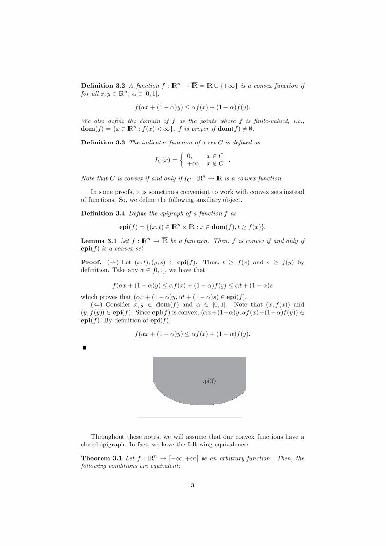
Definition 3.4 Define the epigraph of a function f as

epi(f) = {(x, t) ∈ IRn × IR : x ∈ dom(f), t ≥ f(x)}.Lemma 3.1 Let f : IRn → IR be a function. Then, f is convex if and only ifepi(f) is a convex set.

Proof. (⇒) Let (x, t), (y, s) ∈ epi(f). Thus, t ≥ f(x) and s ≥ f(y) bydefinition. Take any α ∈ [0, 1], we have that

f(αx + (1− α)y) ≤ αf(x) + (1− α)f(y) ≤ αt + (1− α)s

which proves that (αx + (1− α)y, αt + (1− α)s) ∈ epi(f).(⇐) Consider x, y ∈ dom(f) and α ∈ [0, 1]. Note that (x, f(x)) and

(y, f(y)) ∈ epi(f). Since epi(f) is convex, (αx+(1−α)y, αf(x)+(1−α)f(y)) ∈epi(f). By definition of epi(f),

f(αx + (1− α)y) ≤ αf(x) + (1− α)f(y).

Throughout these notes, we will assume that our convex functions have aclosed epigraph. In fact, we have the following equivalence:

Theorem 3.1 Let f : IRn → [−∞, +∞] be an arbitrary function. Then, thefollowing conditions are equivalent:

3

(i) f is lower semi-continuous throughout IRn;

(ii) {x ∈ IRn|f(x) ≤ α} is closed for every α ∈ IR;

(iii) The epigraph of f is a closed set in IRn+1.

We also state some basic facts from Convex Analysis Theory that can befound in [11].

Theorem 3.2 Let f : IRn → IR be a convex function. Then, f is continuous inint dom(f).

4 The Subdifferential of a Convex Function

Now, we define one of the main object of our theory, the subdifferential of aconvex function. Later, we will also prove some additional results about thesubdifferential that we do not use but are very insightful.

Definition 4.1 The subdifferential of a convex function f : IRn → IR at a pointx is defined as

∂f(x) = {s ∈ IRn : f(y) ≥ f(x) + 〈s, y − x〉 for all y ∈ IRn}.

Remark 4.1 We point out that the subdifferential is a set of linear functionals,so it lives on the dual space of the space that contains dom(f). In the case ofIRn we do have an one-to-one correspondence between the dual space and theoriginal space.

Lemma 4.1 Let f : IRn → IR be a convex function, and x ∈ int dom(f).Then, ∂f(x) 6= ∅.

Proof. Since f is convex, epi(f) is also convex. Also, x ∈ dom(f) implies thatf(x) < ∞.

Using the Hahn-Banach Theorem7 there exists a linear functional in s =(s, sn+1) ∈ IRn × IR such that

〈s, (x, f(x))〉 ≤ 〈s, (y, t)〉 for all (y, t) ∈ epi(f),

where the “extended” scalar product is defined as 〈(s, sn+1), (x, t)〉 = 〈s, x〉 +sn+1t.

We need to consider three cases for sn+1.If sn+1 < 0, we have that

〈s, x〉 − |sn+1|f(x) ≤ 〈s, y〉 − |sn+1|t for all (y, t) ∈ epi(f).

Letting t ↗ +∞ we obtain a contradiction since the left hand side is aconstant.

If sn+1 = 0, we have that

〈s, x〉 ≤ 〈s, y〉 for all y ∈ dom(f).

7The version of the Separating Hyperplane Theorem for convex sets.

4

Noting that x ∈ int dom(f), this is also a contradiction and we can also rejectthis case.

So, sn+1 > 0, and due to homogeneity, we can assume sn+1 = 1. Bydefinition of the epigraph, (y, f(y)) ∈ epi(f) for all y ∈ dom(f), which impliesthat

〈s, x〉+ f(x) ≤ 〈s, y〉+ f(y) ∴ f(y) ≥ f(x) + 〈−s, y − x〉 .

Thus, (−s) ∈ ∂f(x).

Example 4.1 We cannot relax the assumption of x ∈ int dom(f) in general.f(x) = −√x is a convex function on IR+, but ∂f(0) = ∅. Note that we alwayshave that

int dom(f) ⊆ dom(∂f) ⊆ dom(f).

At this point, it is useful to stop and relate the subdifferential to the regularcase where f is differentiable.

Lemma 4.2 Let f : IRn → IR be differentiable at x. Then, ∂f(x) = {∇f(x)}.

Proof. Take s ∈ ∂f(x) and an arbitrary d ∈ IRn and t > 0. By definition,

f(x + td) ≥ f(x) + 〈s, x + td− x〉 = f(x) + t 〈s, d〉

Thus,f(x + td)− f(x)

t≥ 〈s, d〉. Now, letting t ↘ 0, the left hand side has a

unique limit since x is differentiable. Finally,

〈∇f(x), d〉 ≥ 〈s, d〉 for all d ∈ IRn,

which implies that s = ∇f(x).The proof of the last Lemma shows that the subgradients are coming from all

the possible partial derivatives. In general, the subdifferential is not a functionas the gradient is for differentiable functions. ∂f is a correspondence, a point-setmapping.

Example 4.2 Consider the function f(x) = |x| for x ∈ IR. The subdifferentialof f in this example is

∂f(x) =

−1, x < 01, x > 0

[−1, 1] , x = 0.

5

We obeserve that at zero, where the function fails to be differentiable, we havemany possible values for subgradients.

Definition 4.2 Let M : IRn → B(IRn) be a point-set mapping. M is said to beupper semi-continuous if for every convergent sequence (xk, sk) → (x, s) suchthat sk ∈ M(xk) for every k ∈ IN, we have that s ∈ M(x). M is said to be lowersemi-continuous if for every s ∈ M(x) and every sequence xk → x, there existsa sequence {yk}k≥1 such that yk ∈ M(xk) and yk → y. Finally, M is said to becontinuous if it is both upper and lower semi-continuous.

Remark 4.2 Another important notion of continuity for point-set mappingsare inner and outter continuity. In finite dimensional spaces, this notion coin-cides with our lower and upper continuity definitions.

The study of the subdifferential through the eyes of the theory of correspon-dences clarifies some important properties and difficulties of working with thatoperator.

Lemma 4.3 The subdifferential of a proper convex function f is upper semi-continuous and convex valued.

Proof. Consider a sequence (xk, sk) → (x, s) where sk ∈ ∂f(xk). Thus, forevery k ∈ IN and every y ∈ IRn,

f(y) ≥ f(xk) +⟨sk, y − xk

⟩

Taking limits, f(xk) → f ≥ f(x), and we obtain

f(y) ≥ f(x) + 〈s, y − x〉 .

Thus, s ∈ ∂f(x).For the second statement, let s1, s2 ∈ ∂f(x), α ∈ [0, 1], and the result follows

since the 〈·, ·〉 is a linear operator.

Example 4.3 From our Example 4.2, it is easy to see that the subdifferentialcan fail to be lower semi-continuous. For instance, take (x, s) = (0, 0) andxk = 1

k . The sequence of {sk} must be chosen to be identically equal to 1 whichis not converging to zero.

In order to introduce an equivalent characterization of the subdifferential off , we need the following lemma.

6

Lemma 4.4 Let f : IRn → IR be a proper lower semicontinuous convex func-tion. Then, the directional derivatives of f are well defined for every d ∈ IRn,

f ′(x; d) = limt↘0

f(x + td)− f(x)t

.

Proof. Let 0 < t′ < t. Thus, let α = t′t so that

x + t′d = α(x + td) + (1− α)x.

Using the convexity of f ,

f(x + t′d)− f(x)t′

=f(α(x + td) + (1− α)x)− f(x)

αt≤ αf(x + td) + (1− α)f(x)− f(x)

αt

=α

α

f(x + td)− f(x)t

,

so the ratio is non increasing in t. Thus, as a monotonic sequence its limit(possibly +∞) is well defined.

Even though the directional derivaties are a local characteristic, it does havesome global properties due to the convexity of f . This is illustraded by thefollowing alternative definition of the subdifferential of f .

Lemma 4.5 The subdifferential of f at x can be written as

∂f(x) = {s ∈ IRn : f ′(x; d) ≥ 〈s, d〉 for every d ∈ IRn} (1)

Proof. By definition, s ∈ ∂f(x) if and only if

f(y) ≥ f(x) + 〈s, y − x〉 for every y ∈ IRn

f(x + td) ≥ f(x) + 〈s, td〉 for every d ∈ IRn and t > 0f(x+td)−f(x)

t ≥ 〈s, d〉 for every d ∈ IRn and t > 0.

Since the left hand side is decreasing as t → 0 by Lemma 4.4,

∂f(x) = {s ∈ IRn : f ′(x; d) ≥ 〈s, d〉 for every d ∈ IRn}.

Thus, the directional derivatives at x bound all the projections of subgradi-ents, in the subdifferential of f at x, on the corresponding direction. The nextresult establish the converse.

Theorem 4.1 Let f : IRn → IR be a lower semi-continuous convex function. Ifx ∈ dom(f),

f ′(x; d) = max{〈s, d〉 : s ∈ ∂f(x)}.

Proof. Without loss of generality, assume that x = 0, f(x) = 0 and ‖d‖ = 1.Denote d := d1, and let {d1, d2, . . . , dn} be an orthogonal basis for IRn. LetHk = span{d1, d2, . . . , dk}.

We start by defining a linear functional on H1, λ1 : H1 → IR as

λ1(y) = f(x) + 〈f ′(x; d)d, y − x〉 .

7

Using Lemma 4.4, for t > 0

f(x + td)− f(x) ≥ tf ′(x; d) = t 〈f ′(x; d)d, d〉 = λ1(x + td)− f(x).

Assume that there exists t > 0 such that f(x − |t|d) < λ1(x − |t|d). Byconvexity, for any t ∈ (0, t ],

f(x− |t|d) ≤( |t||t|

)f(x− |t|d) +

(1− |t|

|t|)

f(x)

<

( |t||t|

)λ1(x− |t|d) +

(1− |t|

|t|)

λ1(x)

= λ1(x− |t|d).

So,

f ′(x;−d) = limt→0f(x−|t|d)−f(x)

t ≤ limt→0λ1(x−|t|d)−f(x)

t

= limt→0f(x)+〈f ′(x;d)d,−|t|d〉−f(x)

t= −f ′(x; d).

If f ′(x;−d) = −f ′(x; d), f : H1 → IR is differentiable at x with gradientequal to f ′(x; d), and using Lemma 4.2, we proved that f(y) ≥ λ1(y) for ally ∈ H1.

Thus, we can assume that f ′(x;−d) < −f ′(x; d). Also, due to Lemma 4.4,we can write that

f(x−|t|d) = f(x)+|t|f ′(x;−d)+o(|t|) and f(x+|t|d) = f(x)+|t|f ′(x; d)+o(|t|).To obtain that

f(x) ≤ 12f(x− |t|d) + 1

2f(x + |t|d)= 1

2 (f(x) + |t|f ′(x;−d) + o(|t|) + f(x) + |t|f ′(x; d) + o(|t|))= f(x) + |t|

2 (f ′(x;−d) + f ′(x; d)) + o(|t|)< f(x),

if we make t small enough since f ′(x;−d)+f ′(x; d) < 0. This is a contradiction.So, for every t ∈ IR, we have f(x + td) ≥ λ1(x + td).

After the construction of the first step, we will proceed by induction. Assumethat for k < n, we have a function λk : Hk → IR such that

λk(x) = f(x), and λk(y) ≥ f(y) for all y ∈ Hk.

Assuming f(x) = 0 for convenience, we have that λk is a linear function, andlet z = dk+1

‖dk+1‖ .Suppose w, v ∈ Hk and α > 0, β > 0.

βλk(w) + αλk(v) = λk(βw + αv)= (α + β)λk

(β

α+β w + αα+β v

)

≤ (α + β)f(

βα+β w + α

α+β v)

= (α + β)f([

βα+β

](w − αz) +

[α

α+β

](v + βz)

)

≤ βf(w − αz) + αf(v + βz).

8

Thus,

β [−f(w − αz) + λk(w)] ≤ α [f(v + βz)− λk(v)]

1α

[−f(w − αz) + λ(w)] ≤ 1β

[f(v + βz)− λk(v)]

supw∈Hk,α>0

1α

[−f(w − αz) + λk(w)] ≤ a ≤ infv∈Hk,β>0

1β

[f(v + βz)− λk(v)]

We extend λk to Hk+1 by defining λk+1(z) = a. Thus, assuming t > 0,

λk+1(tz + x) = tλk+1(z) + λk+1(x) = ta + λk(tx)≤ t

(1t f(x + tz)− λk(x)

t

)+ λk(x)

≤ f(tz + x),

and the case of t < 0 is similar.So, the gradient of λn will define an element s ∈ ∂f(x). Note that

max{〈s, d〉 : s ∈ ∂f(x)} ≥ 〈s, d〉 =

⟨n∑

i=1

αidi, d

⟩= f ′(x; d),

where the last equality follows by the construction of λ1.We finish this section with an easy but useful lemma regarding sums of

functions

Lemma 4.6 Let f1 : IRn → IR and f2 : IRn → IR be two convex functions. Ifx ∈ int dom(f1) ∩ int dom(f2) 6= ∅, then,

∂f1(x) + ∂f2(x) = ∂(f1 + f2)(x).

Proof. (⊆)Let x ∈ int dom(f1) ∩ int dom(f2) 6= ∅ and si ∈ ∂fi(x), i = 1, 2.Then

fi(y) ≥ fi(x) +⟨si, y − x

⟩

and,f1(y) + f2(y) ≥ f1(x) + f2(x) +

⟨s1 + s2, y − x

⟩.

(⊇) Let f := f1 + f2, and take s ∈ ∂f(x), and let H = ∂f1(x) + ∂f2(x).Since x ∈ int dom(f), we have that ∂f1(x) and ∂f2(x) are bounded, closedand convex sets. Thus, since H is a closed convex set. Using the SeparatingHyperplane, there exists d, ‖d‖ = 1, such that

〈s, d〉 > 〈ss, d〉 for all ss ∈ H.

Since x ∈ int dom(f1)∩ int dom(f2), there exists η > 0 such that x+ηd ∈int dom(f1)∩ int dom(f2). Since f is convex, we can compute the directionalderivatives

(f1 + f2)′(x; d) = limt→0f1(x+td)+f2(x+td)−f1(x)−f2(x)

t

= limt→0f1(x+td)−f1(x)

t + limt→0f2(x+td)−f2(x)

t= f ′1(x; d) + f ′2(x; d).

9

Combining this with Theorem 4.1, we have that

max{〈s, d〉 : s ∈ ∂(f1 + f2)(x)} = max{〈s, d〉 : s ∈ ∂f1(x) + ∂f2(x)}

A contradiction since s ∈ ∂(f1 + f2)(x) such that 〈s, d〉 > f ′1(x; d)+ f ′2(x; d).

5 The ε-Subdifferential of a Convex Function

Additional theoretical work is needed to recover the lower semi-continuity prop-erty. We will construct an approximation of the subdifferential which has betterproperties. Among these properties, we will be able to prove the continuity ofour new point-set mapping.

Definition 5.1 For any ε > 0, the ε-subdifferential of a convex function f :IRn → IR at a point x is the point-to-set mapping

∂εf(x) = {s ∈ IRn : f(y) ≥ f(x) + 〈s, y − x〉 − ε, for all y ∈ IRn}.

Remark 5.1 For any ε > 0, the following properties are easy to verify:

• ∂f(x) ⊆ ∂εf(x);

• ∂εf(x) is a closed convex set;

• ∂f(x) =⋂ε>0

∂εf(x);

Now, we will revisit Example 4.2.

Example 5.1 Let f(x) = |x| with x ∈ IR and let ε > 0 be fixed. By definition,

∂εf(x) = {s ∈ IR : |y| ≥ |x|+ s(y − x)− ε, for all y ∈ IR}

First consider y − x > 0. Then,

s ≤ |y| − |x|+ ε

y − x⇒ s ≤

{1, x > 0

−1 + ε−x , x < 0

On the other hand, if y − x < 0 we have that,

s ≥ |y| − |x|+ ε

y − x⇒ s ≥

{ −1, x > 01− ε

x , x < 0

obtaining

∂εf(x) =

[−1,−1− εx

], x < − ε

2[−1, 1] , x ∈ [

ε2 , ε

2

][1, 1− ε

x

], x > ε

2

10

Before addressing the continuity of the operator, we answer the question ofwhether a subgradient at a some point is an approximation for subgradients atanother point.

Proposition 5.1 Let x, x′ ∈ dom(f), and s′ ∈ ∂f(x′). Then,

s′ ∈ ∂εf(x) if and only if f(x′) ≥ f(x) + 〈s′, x′ − x〉 − ε.

Proof. (⇒) From the definition of ∂εf(x) using y = x′.(⇐) Since s′ ∈ ∂f(x′),

f(y) ≥ f(x′) + 〈s′, y − x′〉= f(x) + 〈s′, y − x〉+ [f(x′)− f(x) + 〈s′, x− x′〉]≥ f(x) + 〈s′, y − x〉 − ε

where the last inequality follows from the assumption. So, s′ ∈ ∂εf(x).This motivates the following definition, which will play an important role in

the Bundle Methods to be defined later.

Definition 5.2 For a triple (x, x′, s′) ∈ dom(f)×dom(f)× IRn, the lineariza-tion error made at x, when f is linearized at x′ with slope s′, is the number

e(x, x′, s′) := f(x)− f(x′)− 〈s′, x− x′〉 .

Corollary 5.1 Let s′ ∈ ∂ηf(x′). Then, s′ ∈ ∂εf(x) iff(x′) ≥ f(x) + 〈s′, x′ − x〉 − ε + η or, equivalently, e(x, x′, s′) + η ≤ ε.

11

6 Continuity of ∂εf(·)This section proves the continuity of the ε-subdifferential. To do so, we willneed the following lemma:

Lemma 6.1 Assume that dom(f) 6= ∅, δ > 0, and B(x, δ) ⊆ int dom(f). If fis L-Lipschitzian on B(x, δ), then, for any δ′ < δ, s ∈ ∂εf(y), and y ∈ B(x, δ′),we have that

‖s‖ < L +ε

δ − δ′

Proof. Assume s 6= 0 and let z := y + (δ − δ′)s

‖s‖ . By definition of s ∈ ∂εf(y)

f(z) ≥ f(y) + 〈s, z − y〉 − ε

Now, note that z ∈ B(x, δ) and y ∈ B(x, δ). Thus, the Lipschitz constant Lholds and we obtain that

L‖z − y‖ ≥ f(z)− f(y) ≥ 〈s, z − y〉 − ε

Using that ‖z − y‖ = ‖(δ − δ′)s

‖s‖‖ = (δ − δ′),

(δ − δ′)L ≥⟨

s, (δ − δ′)s

‖s‖⟩− ε = ‖s‖(δ − δ′)− ε

we obtain the desired inequality.

Theorem 6.1 Let f : IRn → IR be a convex Lipschitz function on IRn. Then,there exists a constant K > 0 such that for all x, x′ ∈ IRn, ε, ε′ > 0, s ∈ ∂εf(x),there exists s′ ∈ ∂ε′f(x′) satisfying

‖s− s′‖ ≤ K

min{ε, ε′} (‖x− x′‖+ |ε− ε′|)

Proof. Since ∂εf(x) and ∂ε′f(x) are convex sets8, it is sufficient to show thatfor every d,

max{〈s, d〉 : s ∈ ∂εf(x)}−max{〈s′, d〉 : s′ ∈ ∂ε′f(x)} <K (‖x− x′‖+ |ε− ε′|)

min{ε, ε′} .

So, we will fix a vector d, ‖d‖ = 1. Define the ε-directional derivate9 of f at xin d as,

f ′ε(x; d) := inft>0

f(x + td)− f(x) + ε

t, (2)

where the quotient on the right hand side will be denoted by

qε(x, t) =f(x + td)− f(x) + ε

t.

8Otherwise we could separate a point s ∈ ∂εf(x) from ∂ε′f(x) using the Separating Hy-perplane

9Note that the definition does not involve the limt→0. It is the infimum of the values ofthe quocients qε(x, t).

12

We note that Theorem 4.1 can be adapted to prove

f ′ε(x; d) = max{〈s, d〉 : s ∈ ∂εf(x)}.

For any η > 0, there exists tη > 0 such that

qε(x, tη) ≤ f ′ε(x, d) + η (3)

Using Lemma 6.1 with δ ↗∞, we have that f ′ε(x, d) ≤ L, and so qε(x, t) <L + η. On the other hand,

qε(x, tη) =f(x + tηd)− f(x) + ε

tη≥ −L +

ε

tη

Therefore,

1tη≤ 2L + η

ε. (4)

Thus, using Equations (2) and (3)

f ′ε′(x′; d)− f ′ε(x; d)− η ≤ qε′(x′, tη)− qε(x, tη)

=f(x′ + tηd)− f(x + tηd) + f(x)− f(x′) + ε′ − ε

tη

≤ 2L‖x− x′‖+ |ε− ε′|tη

≤ 2L + η

ε(2L‖x− x′‖+ |ε− ε′|)

where the last inequality is obtained using Equation (4). Also, since η > 0 isarbitrary and one can interchange x and x′, we obtain

|f ′ε′(x′; d)− f ′ε(x; d)| ≤ 2L

min{ε, ε′} (2L‖x− x′‖+ |ε′ − ε|)

The constant of interest can be chosen to be K = max{2L, 4L2}.

Corollary 6.1 The correspondence M : IRn × IR++ → B(IRn) defined by

(x, ε) 7→ ∂εf(x)

is a continuous correspondence.

Proof. The previous Lemma establishes the lower semi-continuity for any ε > 0.The upper semi-continuity follows directly from f being lower semi-continuous.

Take a sequence (xk, sk, εk) → (x, s, ε), then for all y ∈ IRn,

f(y) ≥ f(xk) +⟨sk, y − xk

⟩− εk for every k.

Since f is lower semi-continuous, taking the limit of k →∞,

f(y) ≥ f(x) + 〈s, y − x〉 − ε for every y ∈ IRn.

Thus, s ∈ ∂εf(x) and M is upper semi-continuous.

13

Example 6.1

7 Motivation through the Moreau-Yosida Reg-ularization

Let f : IRn → IR be a proper convex function. We define the Moreau-Yosidaregularization of f for a fixed λ > 0 as

F (x) = miny∈IRn

{f(y) +

λ

2‖y − x‖2

}.

p(x) = arg miny∈IRn

{f(y) +

λ

2‖y − x‖2

}.

The proximal point p(x) is well defined since the function being minimized isstrictly convex.

Proposition 7.1 If f : IRn → IR be a proper convex function, then F is afinite-valued, convex and everywhere differentiable function with gradient givenby

∇F (x) = λ(x− p(x)).

Moreover,

‖∇F (x)−∇F (x′)‖2 ≤ λ 〈∇F (x)−∇F (x′), x− x′〉 for all x, x′ ∈ IRn

and‖∇F (x)−∇F (x′)‖ ≤ λ‖x− x′‖ for all x, x′ ∈ IRn.

14

Proof.(Finite-valued). If f is a proper function, there exists x ∈ IRn such that

f(x) < ∞. Thus, F is finite-valued since

F (x′) ≤ f(x) +λ

2‖x− x′‖2 < ∞.

(Convexity).Take x, x′ ∈ IRn, and α ∈ [0, 1], then

αF (x) + (1− α)F (x′) = αf(p(x)) + (1− α)f(p(x′)) + λ2

(α‖p(x)− x‖2 + (1− α)‖p(x′)− x′‖2)

≥ f(αp(x) + (1− α)p(x′)) + λ2 ‖αp(x) + (1− α)p(x′)− (αx + (1− α)x′)‖2

≥ F (αx + (1− α)x′)

(Differentiability). Fix an arbitrary direction d, ‖d‖ = 1, and let t > 0. Bydefinition

F (x+td)−F (x)t =

miny

[f(y) + λ

2 ‖y − x− td‖2]−minw

[f(w) + λ

2 ‖w − x‖2]

t

≥[f(p(x + td)) + λ

2 ‖p(x + td)− x− td‖2]− [f(p(x + td)) + λ

2 ‖p(x + td)− x‖2]

t

=λ

2‖p(x + td)− x− td‖2 − ‖p(x + td)− x‖2

t

=λ

2‖p(x + td)− p(x) + p(x)− x− td‖2 − ‖p(x + td)− p(x) + p(x)− x‖2

t

=λ

2‖p(x)− x− td‖2 − ‖p(x)− x‖2

t− λ 〈p(x + td)− p(x), d〉

where we used that F (x) ≤ f(p(x + td)) + λ2 ‖p(x + td)− x‖2. Now, taking the

limit as t → 0, p(x + td) → p(x) implies that

limt→0

F (x + td)− F (x)t

≥ 〈λ(x− p(x)), d〉 .

On the other hand, since F (x + td) ≤ f(p(x)) + λ2 ‖p(x)− x− td‖2,

F (x+td)−F (x)t =

miny

[f(y) + λ

2 ‖y − x− td‖2]−minw

[f(w) + λ

2 ‖w − x‖2]

t

≤[f(p(x)) + λ

2 ‖p(x)− x− td‖2]− [f(p(x)) + λ

2 ‖p(x)− x‖2]

t

=λ

2‖p(x)− x− td‖2 − ‖p(x)− x‖2

t

Again, taking the limit t → 0,

limt→0

F (x + td)− F (x)t

≤ 〈λ(x− p(x)), d〉 .

‖∇F (x)−∇F (x′)‖2 = λ 〈∇F (x)−∇F (x′), x− p(x)− x′ + p(x′)〉= λ 〈∇F (x)−∇F (x′), x− x′〉+ λ 〈∇F (x)−∇F (x′), p(x′)− p(x)〉

We will prove that the last term is negative. To do so, we need the follow-ing (known as the monotonicity of ∂f(x)). Let s ∈ ∂f(x) and s′ ∈ ∂f(x′),

15

then 〈s− s′, x− x′〉 ≥ 0. To prove that, consider the subgradient inequalitiesassociated with s and s′ applied to x′ and x respectively,

f(x′) ≥ f(x) + 〈s, x′ − x〉 and f(x) ≥ f(x′) + 〈s, x′ − x〉 .Adding these inequalities we obtain 〈s− s′, x− x′〉 ≥ 0.

Now, note that by optimality of p(x) and p(x′),

0 ∈ ∂

(f(p(x)) +

λ

2‖p(x)− x‖2

)and 0 ∈ ∂

(f(p(x′)) +

λ

2‖p(x′)− x′‖2

).

So, ∇F (x) = λ(x − p(x)) ∈ ∂f(p(x)) and ∇F (x′) = λ(x′ − p(x′)) ∈ ∂f(p(x′)).Using the monotonicity of ∂f ,

〈∇F (x)−∇F (x′), p(x′)− p(x)〉 ≤ 0.

The proof of the last inequality follows directly from the previous result,

‖∇F (x)−∇F (x′)‖2 ≤ λ 〈∇F (x)−∇F (x′), x− x′〉 ≤ λ‖∇F (x)−∇F (x′)‖‖x−x′‖Therefore, ‖∇F (x)−∇F (x′)‖ ≤ λ‖x− x′‖.

We finish this section with a characterization of points of minimum of f andits regularization F .

Proposition 7.2 The following statements are equivalent:

(i) x ∈ arg min{f(y) : y ∈ IRn};(ii) x = p(x);

(iii) ∇F (x) = 0;

(iv) x ∈ arg min{F (y) : y ∈ IRn};(v) f(x) = f(p(x));

(vi) f(x) = F (x);

Proof.(i) ⇒ (ii) f(x) = f(x) + λ

2 ‖x− x‖2 ≤ f(y) + λ2 ‖y − x‖2 ⇒ p(x) = x.

(ii) ⇔ (iii) x = p(x) ⇔ ∇F (x) = λ(x− p(x)) = 0.

(iii) ⇔ (iv) Since F is convex, ∇F (x) = 0 ⇔ x ∈ arg min{F (y) : y ∈ IRn}.

(iv) ⇒ (v) Using (ii), x = p(x) implies that f(x) = f(p(x)).

(v) ⇒ (vi) f(x) = f(p(x)) ≤ f(p(x)) + λ2 ‖p(x)− x‖2 = F (x) ≤ f(x).

(vi) ⇒ (i) F (x) = f(x) implies that p(x) = x. Thus,

0 ∈ ∂f(x) + λ(x− p(x)) = ∂f(x).

Remark 7.1 During the past ten years, several authors tried to introduce sec-ond order information via the Moreau-Yosida regularization. It is possible toshow that the Hessian ∇2F (x) exists if and only if the Jacobian ∇p(x) existsobtaining

∇2F (x) = λ (I −∇p(x)) for all x ∈ IRn.

16

8 Nondifferentiable Optimization Methods

In the next section, we will state a Bundle Method for minimizing a convexfunction f : IRn → IR given only by an oracle. Before proceeding to discuss theBundle Methods in detail, we introduce two other methods which will contex-tualize the Bundle Method in the literature.

8.1 Subgradient Method

This is probably the most used method for nondifferentiable convex optimiza-tion. Basically, it consists of replacing gradients with subgradients in the clas-sical steepest descent method.

Subgradient Method (SM)

Step 1. Start with a x0, set k = 0 and a tolerance ε > 0.

Step 2. Compute f(xk) and a subgradient sk ∈ ∂f(xk).

Step 3. If ‖sk‖ < ε, stop.

Step 4. Define a stepsize θk > 0.

Step 5. Define xk+1 = xk − θksk

‖sk‖ .

Step 6. Set k = k + 1, and goto Step 2.

We refer to [12] for a detailed study. The choice of the sequence {θk} is cru-cial in the performance of this algorithm. There are choices which convergenceis guaranteed. Let θk → 0 and

∑k≥1 θk = ∞. Then, f(xk) → f∗ the optimal

value. Moreover, if in addition the stepsize sequence satisfies∑

k≥1(θk)2 < ∞,

we have that xk → x a solution of the problem10. Several other rules have beenproposed to speed up convergence especially when bounds on the optimal valueare available.

An important difference between the differentiable case and the non-differentiablecase concerns descent directions and line searches. A direction opposite to a par-ticular subgradient does not need to be a descent direction (as opposed to minusthe gradient for the differentiable case). In fact, a vector d is a descent directionfor f at x only if

〈d, s〉 < 0 for all s ∈ ∂f(x).

10Note that the second condition automatically implies in sublinear convergence.

17

Thus, traditional line searches first proposed for differentiable functions mustbe adapted before being applied.

Finally, the stopping criterion is too strict here. As illustrated by Example4.2, this criterion may never be met even if we are at the solution.

8.2 Cutting Planes Method

The simplicity of the previous algorithm comes at the price of ignoring pastinformation. The information obtained by the oracle can be used to build notonly descent directions, but also a model of the function f itself. This is alsobe used in the Bundle Methods but was first developed by the Cutting PlaneMethod.

Consider the bundle of information formed by {yi, f(yi), si ∈ ∂f(yi)}`i=1.

Remembering that for all y ∈ IRn and i = 1, . . . , `,

f(y) ≥ f(yi) +⟨si, y − yi

⟩,

we can construct the following piecewise-linear approximation of f ,

f`(y) := maxi=1,...,`

f(yi) +⟨si, y − yi

⟩. (5)

By construction, we have that f`(y) ≤ f(y) for all y ∈ IRn. Also, it is clearthat f`(y) ≤ f`+1(y) for all y ∈ IRn. There are at least two motivations forthis cutting-plane model. First, it can be modelled by linear constraints, sooptimizing the model reduces to a LP. The second motivation is the followinglemma.

Lemma 8.1 Let f be any lower semicontinuous convex function. Denote byHf the set of affine functions minoring f , formally defined as

Hf = {h : IRn → IR : h is an affine function such that h(y) ≤ f(y) for all y ∈ IRn}.

Then,

f(x) = sup{h(x) : h ∈ Hf} and ∂f(x) = {∇h(x) : h(x) = f(x), h ∈ Hf}.

18

Proof. The epigraph of f is closed. So, any point (x, t) /∈ epi(f), can be strictlyseparated by an affine hyperplane h(x,t) : IRn × IR → IR, defined as

h(x,t)(y, s) = 〈sx, x− y〉+ (s− t),

from epi(f). In fact, we can take the supremum over t ≤ f(x) and to obtain,

hx(y, s) = 〈sx, x− y〉+ s− f(x).

The semi-space Hx = {(y, s) ∈ IRn × IR : hx(y, s) ≥ 0} contains epi(f).Thus, the intersection of all such hyperplanes is a closed convex set containingepi(f) and contained on epi(f) (since any point not in the epigraph can beseparated). The result follows from the fact that arbitrary intersection of theepigraph of lower semicontinuous functions equals the epigraph of the maximumof these functions.

For the second statement, the direction (⊇) is by definition of ∂f(x). Toprove (⊆), note that any s ∈ ∂f(x) induces an affine function

hs(y) = f(x) + 〈s, y − x〉 ,for which holds that hs(x) = f(x) and hs(y) ≤ f(y) for all y ∈ IRn. Thus, hs isincluded in the supremum and ∇hs(x) = s.

In order for the method to be well defined, we still need to specify a compactset C and restrict our model to this set to ensure that every iterate is welldefined.

Cutting Plane Method (CP)

Step 1. Let δ > 0 and consider a convex compact set C containing aminimizing point. Let k = 1, y1 ∈ C, and define f0 ≡ −∞.

Step 2. Compute f(yk) and a subgradient sk ∈ ∂f(yk).

Step 3. Define δk := f(yk)− fk−1(yk) ≥ 0.

Step 4. If δk < δ, stop.

Step 5. Update Model fk(y) := max{fk−1(y), f(xk) +⟨sk, y − yk

⟩}.

Step 6. Compute yk+1 ∈ arg miny∈C fk(y).

Step 7. Set k = k + 1, and goto Step 2.

This method has several advantages when compared with the SubgradientMethod. The model fk−1 provides us with a stopping criterion based on δk

which did not exist for the Subgradient Method. The value of δk is callednominal decrease, the improvement predicted by the model in the objectivefunction for the next iterate yk+1. Since the model satisfies fk(y) ≤ f(y), wehave that

miny

fk(y) ≤ miny

f(y).

Thus, if the stopping criterion is satisfied we have that f(yk) − fk−1(yk) < δimplying that

19

f(yk) < δ + fk(yk) = δ + miny

fk(y) ≤ δ + miny

f(y).

This is achieved at the cost of solving a linear programming on Step 5 inorder to define the next point to be evaluated by the oracle. This definitionof the next iterate also allows the algorithm to perform long steps on eachiteration11.

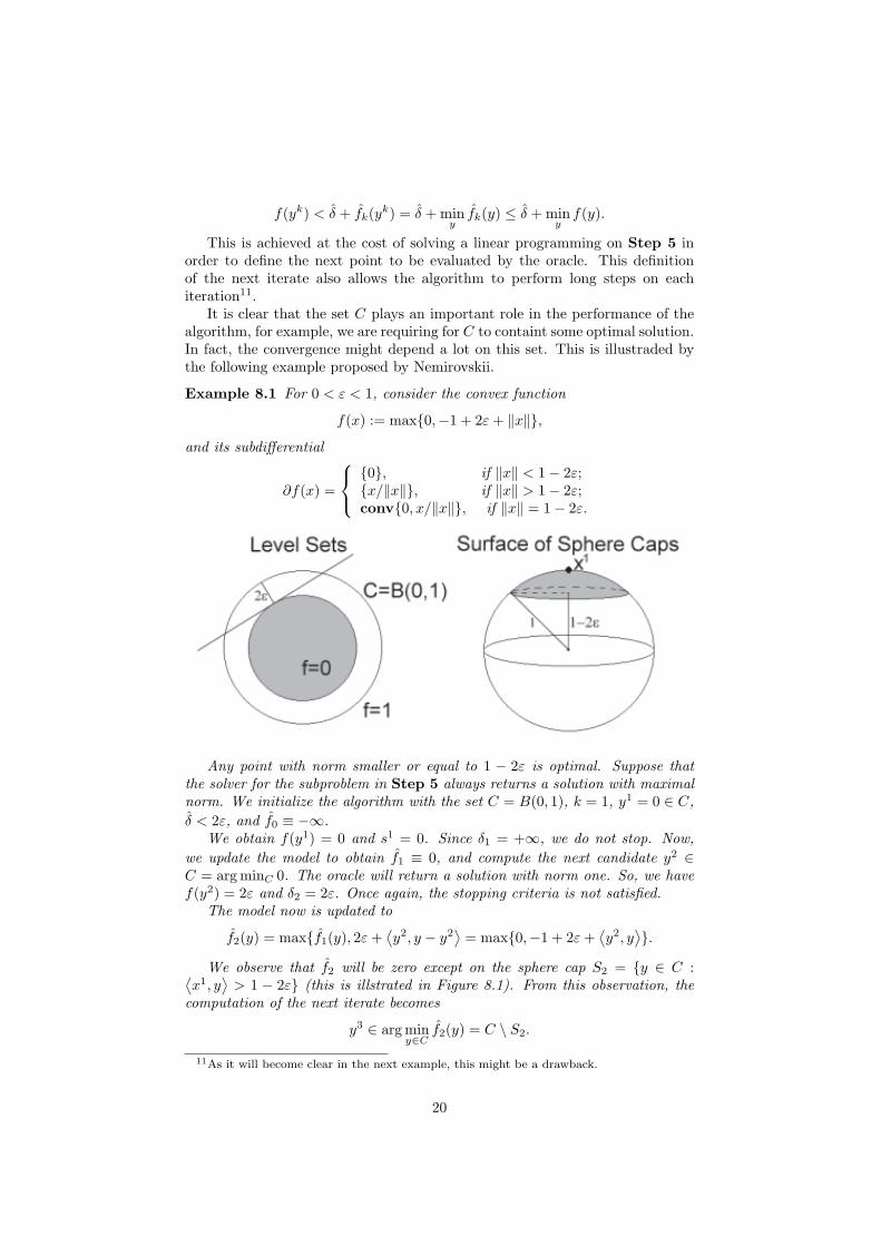
It is clear that the set C plays an important role in the performance of thealgorithm, for example, we are requiring for C to containt some optimal solution.In fact, the convergence might depend a lot on this set. This is illustraded bythe following example proposed by Nemirovskii.

Example 8.1 For 0 < ε < 1, consider the convex function

f(x) := max{0,−1 + 2ε + ‖x‖},and its subdifferential

∂f(x) =

{0}, if ‖x‖ < 1− 2ε;{x/‖x‖}, if ‖x‖ > 1− 2ε;conv{0, x/‖x‖}, if ‖x‖ = 1− 2ε.

Any point with norm smaller or equal to 1 − 2ε is optimal. Suppose thatthe solver for the subproblem in Step 5 always returns a solution with maximalnorm. We initialize the algorithm with the set C = B(0, 1), k = 1, y1 = 0 ∈ C,δ < 2ε, and f0 ≡ −∞.

We obtain f(y1) = 0 and s1 = 0. Since δ1 = +∞, we do not stop. Now,we update the model to obtain f1 ≡ 0, and compute the next candidate y2 ∈C = arg minC 0. The oracle will return a solution with norm one. So, we havef(y2) = 2ε and δ2 = 2ε. Once again, the stopping criteria is not satisfied.

The model now is updated to

f2(y) = max{f1(y), 2ε +⟨y2, y − y2

⟩= max{0,−1 + 2ε +

⟨y2, y

⟩}.We observe that f2 will be zero except on the sphere cap S2 = {y ∈ C :⟨

x1, y⟩

> 1 − 2ε} (this is illstrated in Figure 8.1). From this observation, thecomputation of the next iterate becomes

y3 ∈ arg miny∈C

f2(y) = C \ S2.

11As it will become clear in the next example, this might be a drawback.

20

In the subsequent iterations, another sphere cap (exactly the same up to a ro-tation) will have positive values in the respective model. The next iterate iscomputed as

yk+1 ∈ arg miny∈C

fk(y) = C \k⋃

i=2

Si.

Consequently, as long as there exists vectors with norm one in C \ ⋃ki=2 Si, a

solution with norm one will be returned by the solver, obtaining f(yk+1) = 2εand the algorithm does not stop.

Thus, the Cutting Plane will require at least Voln−1(∂B(0, 1))/Voln−1(∂S2)iterations before terminating. Denote by νn = Voln−1(∂B(0, 1)) the n − 1-dimensional volume of the surface of a n-dimensional sphere,

Voln−1(∂B(0, 1)) = νn = 2νn−1

∫ 1

0

(1−t2)n−1

2 dt ≥ νn−1

∫ 1

0

2t(1−t2)n−1

2 dt ≥ 2n + 1

νn−1,

Voln−1(∂S2) = νn−1

∫ 1

1−2ε

(1−t2)n−1

2 dt ≤ νn−1(1−(1−2ε)2)(n−1)/2(1−(1−2ε))

≤ νn−1

(4ε− 4ε2

)(n+1)/2.

So, we are required to perform at least

Voln−1(∂B(0, 1))Voln−1(∂S2)

≥ 2n + 1

(14ε

)(n+1)/2

.

This is associated with the possibility of performing long steps and possiblegenerating a zig-zag behavior of the iterates. Another important remark to bemade is that the number of constraints in the LP is growing with the numberof iterations.

9 Bundle Methods

Motivated by the theorems in the previous sections, we define another methodwhich can be seen as a stabilization of the Cutting Plane Method.

We start by adding an extra point called the center, xk, to the bundle ofinformation. We will still make use of the same piecewise-linear model for ourfunction, f , but no longer solve an LP on each iteration. Instead, we willcompute the next iterate by computing the Moreau-Yosida regularization for fk

at xk.

Bundle Algorithm (BA)

Step 1. Let δ > 0, m ∈ (0, 1), x0, y0 = x0, and k = 0. Compute f(x0)and s0 ∈ ∂f(x0). Define f0(y) = f(x0) +

⟨s0, y − x0

⟩.

Step 2. Compute the next iterate

yk+1 ∈ arg miny∈IRn

fk(y) +µk

2‖y − xk‖2 (6)

21

Step 3. Define δk := f(xk)−[fk(yk+1) + µk

2 ‖yk+1 − xk‖2]≥ 0.

Step 4. If δk < δ stop.

Step 5. Compute f(yk+1) and a subgradient sk+1 ∈ ∂f(yk+1).

Step 6. If f(xk)− f(yk+1) ≥ mδk, Serious Step (SS) xk+1 = yk+1.

Else, Null Step (NS) xk+1 = xk.

Step 7. Update the Model

fk+1(y) := max{fk(y), f(yk+1) +⟨sk+1, y − yk+1

⟩}.

Step 8. Set k = k + 1, and goto Step 2.

The quadratic term in the relation (6) is responsible for interpreting this as astabilization of the Cutting Planes Method. It will make the next iterate closerto the current center by avoiding drastic movements as in the case of CuttingPlanes. The role of the parameter µk is exactly to control the trade off betweenminimizing the model f and staying close to a point xk which is known to begood.

It will be important to highlight the subsequence of iterations where weperformed a Serious Step. We denote such iterations by Ks = {k ∈ IN :kth iteration was a SS}. We also note that the sequence {f(xk)}k∈Ks is strictlydecreasing due to the Serious Step test in Step 6. The SS test requires that thenew center must improve by at least a fixed fraction m from the improvementδk predicted by the model.

This is a basic version of the method and several enhancements such asline searches, updates of the parameter µk, and other operations may also beincorporated.

9.1 A Dual View

Before we move to convergence proofs, it will be more convenient in theory andpractice to work with the dual of the QP in (6).

Now, we will rewrite our model fk more conveniently. Assuming that ourmodel has ` ≤ k pieces, we define the linearization errors at the center xk to be

ei := f(xk)− [f(yi)− ⟨

si, xk − yi⟩]

for i = 1, . . . , `.

Thus, our model becomes

fk(y) = maxi=1,...,`

{f(yi) +⟨si, y − yi

⟩}= max

i=1,...,`{f(xk)− ei −

⟨si, xk − yi

⟩+

⟨si, y − yi

⟩}= f(xk) + max

i=1,...,`{−ei +

⟨si, y − xk

⟩}

In fact, our bundle of information can be kept as(xk,

{si, ei

}`

i=1

),

22

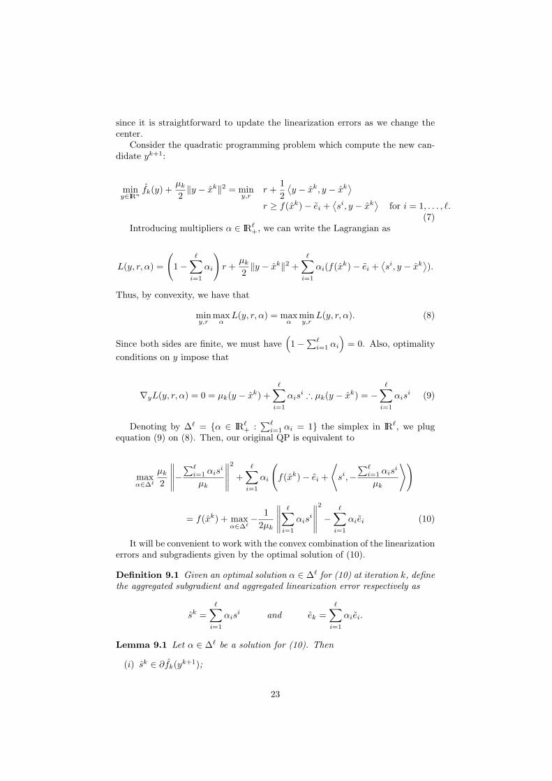
since it is straightforward to update the linearization errors as we change thecenter.

Consider the quadratic programming problem which compute the new can-didate yk+1:

miny∈IRn

fk(y) +µk

2‖y − xk‖2 = min

y,rr +

12

⟨y − xk, y − xk

⟩

r ≥ f(xk)− ei +⟨si, y − xk

⟩for i = 1, . . . , `.

(7)Introducing multipliers α ∈ IR`

+, we can write the Lagrangian as

L(y, r, α) =

(1−

∑

i=1

αi

)r +

µk

2‖y − xk‖2 +

∑

i=1

αi(f(xk)− ei +⟨si, y − xk

⟩).

Thus, by convexity, we have that

miny,r

maxα

L(y, r, α) = maxα

miny,r

L(y, r, α). (8)

Since both sides are finite, we must have(1−∑`

i=1 αi

)= 0. Also, optimality

conditions on y impose that

∇yL(y, r, α) = 0 = µk(y − xk) +∑

i=1

αisi ∴ µk(y − xk) = −

∑

i=1

αisi (9)

Denoting by ∆` = {α ∈ IR`+ :

∑`i=1 αi = 1} the simplex in IR`, we plug

equation (9) on (8). Then, our original QP is equivalent to

maxα∈∆`

µk

2

∥∥∥∥∥−∑`

i=1 αisi

µk

∥∥∥∥∥

2

+∑

i=1

αi

(f(xk)− ei +

⟨si,−

∑`i=1 αis

i

µk

⟩)

= f(xk) + maxα∈∆`

− 12µk

∥∥∥∥∥∑

i=1

αisi

∥∥∥∥∥

2

−∑

i=1

αiei (10)

It will be convenient to work with the convex combination of the linearizationerrors and subgradients given by the optimal solution of (10).

Definition 9.1 Given an optimal solution α ∈ ∆` for (10) at iteration k, definethe aggregated subgradient and aggregated linearization error respectively as

sk =∑

i=1

αisi and ek =

∑

i=1

αiei.

Lemma 9.1 Let α ∈ ∆` be a solution for (10). Then

(i) sk ∈ ∂fk(yk+1);

23

(ii) fk(yk+1) = f(xk)− 1µk

∥∥sk∥∥2 − ek;

(iii) δk = 12µk

‖sk‖2 + ek.

Proof. (i) From equation (9), µk(yk+1 − xk) + sk = 0. So,

−µk(yk+1 − xk) = sk

and since yk+1 is optimal for (6),

0 ∈(∂fk(yk+1) + µk(yk+1 − xk)

)∴ −µk(yk+1 − xk) ∈ ∂fk(yk+1).

(ii) Due to convexity, there is no duality gap between (7) and (10). Thus,

fk(yk+1) +µk

2‖yk+1 − xk‖2 = f(xk)− 1

2µk‖sk‖2 − ek

fk(yk+1) = f(xk)− µk

2

∥∥∥−1µk

sk∥∥∥

2

− 12µk

‖sk‖2 − ek

= f(xk)− 1µk‖sk‖2 − ek.

(iii) Using (ii) in the definition of δk,

δk = f(xk)− fk(yk+1)− µk

2 ‖yk+1 − xk‖2= f(xk)− µk

2 ‖yk+1 − xk‖2 − f(xk) + 1µk‖sk‖2 + ek

= 12µk

‖sk‖2 + ek.

Lemma 9.2 For the aggregated subgradient and linearization error, it holdsthat

sk ∈ ∂ekf(xk).

Proof. Using Lemma 9.1 (i), sk ∈ ∂fk(yk+1), and by construction f ≥ fk.Therefore,

f(y) ≥ fk(y) ≥ fk(yk+1) +⟨sk, y − yk+1

⟩= f(xk)− 1

µk‖sk‖2 − ek +

⟨sk, y − xk + xk − yk+1

⟩

= f(xk) +⟨sk, y − xk

⟩− ek +⟨sk, xk − yk+1

⟩− 1µk‖sk‖2

= f(xk) +⟨sk, y − xk

⟩− ek,

where we used that xk − yk+1 = 1µk

sk.Lemmas 9.1 and 9.2 motivates our convergence proofs in the next section.

If we manage to prove that δk → 0, we also proved that ‖sk‖ → 0 and ek → 0(as long as the parameter µk is bounded). On the other hand, sk ∈ ∂ek

f(xk).So, if xk → x, we obtain that 0 ∈ ∂f(x) since the underlying correspondence isupper semi-continuous.

24

9.2 Aggregation

In the Cutting Plane Method, the number of constraints in the linear program-ming problem is growing with the number of iterations. This is associated withthe model fk, so we are subject to the same problem in the context of BundleMethods. In fact, since we need to solve a quadratic probramming problem, wehave a potentially more serious problem to deal with.

In order to avoid this problem, we can introduce an additional Step in (BA).Based on the optimal solution of (10), we will discard at least two linear pieces ofour model, and introduce the gradient associated with the next iterate and an-other piece based on the aggregated subgradient and linearization error. Definethe aggregated linear piece as

fa(y) = f(xk) +⟨sk, y − xk

⟩− ek. (11)

Lemma 9.3 For fa defined by (11), it holds that

(i) fa(y) = fk(yk+1) +⟨sk, y − yk+1

⟩,

(ii) fa(y) ≤ fk(y).

Proof. (i) Using Lemma 9.1 (ii),

fa(y) = f(xk) +⟨sk, y − yk+1

⟩+

⟨sk, yk+1 − xk

⟩− ek

= f(xk) +⟨sk, y − yk+1

⟩+

⟨sk, −sk

µk

⟩+ fk(yk+1)− f(xk) + 1

µk‖sk‖2

= fk(yk+1) +⟨sk, y − yk+1

⟩.

(ii) fa(y) = f(xk) +⟨sk, y − xk

⟩− ek

= f(xk) +∑`

i=1 αi

(−ei +⟨si, y − xk

⟩)

≤ fk(yk+1) + maxi=1,...,`{−ei +⟨sk, y − xk

⟩} = fk(y).

Lemma 9.4 Take an arbitrary function ψ : IRn → IR such that

ψ(y) ≥ fa(y) for all y ∈ IRn and ψ(yk+1) = fa(yk+1)

Then,yk+1 = arg min

y∈IRnψ(y) +

µk

2‖y − xk‖2.

Proof. Using Lemma 9.3 (i),

ψ(y) + µk

2 ‖y − xk‖2 ≥ fa(y) + µk

2 ‖y − xk‖2= fk(yk+1) +

⟨sk, y − yk+1

⟩+ µk

2 ‖y − xk‖2,

where equality holds if y = yk+1. The optimality conditions for minimizing theright hand side is

µk(y∗ − xk) = −sk.

Thus, y∗ = yk+1, implying that yk+1 minimizes the desired expression.As it will become clear in the convergence proofs, the only properties that

are required by the model are exactly f(yk) = fk(yk) and fk(y) ≥ fa(y).

25

10 Convergence Analysis

In this section, we will assume that the algorithm (BA) is used over a lower-semicontinuous function f , finite-valued on IRn. The general case proofs are similarbut one needs to keep track of the Normal Cone induced by the set dom(f).Here, we will apply (BA) with the parameter δ = 0, that is, (BA) loops forever.Our analysis is divided in two excludent cases:

• (BA) performs an infinite number of Serious Steps, i.e., |Ks| = +∞;

• (BA) performs a finite number of Serious Steps and then only Null Steps.

Lemma 10.1 Consider the (BA) and denote by f = minx f(x) > −∞. Then,

(0 ≤)∑

k∈Ks

δk ≤ f(x0)− f

m< +∞.

Proof. Take k ∈ Ks. Thus, since the SS test was satisfied,

f(xk)− f(yk+1) = f(xk)− f(xk+1) > mδk.

Let k′ be the next index in Ks which is ordered increasingly. Again, by defini-tion,

f(xk′)− f(xk′+1) = f(xk+1)− f(xk′+1) ≥ mδk′ .

Summing over Ks,∑

k∈Ks

mδk ≤∑

k∈Ks

f(xk)− f(xk+1) ≤ f(x0)− f

Lemma 10.2 Suppose that f∗ = limk∈Ks f(xk) > −∞ and |Ks| = ∞.

(i) If∑

k∈Ks

1µk

= ∞, then zero is a cluster point of {sk}k∈Ks , that is, lim inf ‖sk‖ =

0.

(ii) If µk ≥ c > 0 and ∅ 6= arg minx f(x), then {xk}k∈Ks is bounded.

Proof. (i) Using Lemma 9.1 (iii), δk ≥ δk − ek − 12µk

‖sk‖2 ≥ 0.Also, Lemma10.1 states that

∑

k∈Ks

‖sk‖22µk

<∑

k∈Ks

δk ≤ f(x0)− f∗

m.

Thus, sk → 0 over k ∈ Ks.(ii) Let x ∈ arg miny f(y). By definition f(x) ≤ f(y) for all y ∈ IRn. Now,

for k ∈ Ks,

‖x− xk+1‖2 = ‖x− xk‖2 + 2⟨x− xk, xk − xk+1

⟩+ ‖xk − xk+1‖2

= ‖x− xk‖2 + 2µk

⟨x− xk, sk

⟩+ 1

µ2k‖sk‖2

= ‖x− xk‖2 + 2µk

(⟨x− xk, sk

⟩+ 1

2µk‖sk‖2

)

= ‖x− xk‖2 + 2µk

(fk(x)− f(xk) + ek + 1

2µk‖sk‖2

)

≤ ‖x− xk‖2 + 2µk

(f(x)− f(xk) + δk

)

≤ ‖x− xk‖2 + 2µk

δk

26

Thus,

‖x− xk+1‖2 ≤ ‖x− x0‖2 + 2k+1∑

i=1

δi

µi≤ ‖x− x0‖2 +

2c

∑

k∈Ks

δk

which is bounded by Lemma 10.1. Thus, {xk}k∈Ks is bounded.

Theorem 10.1 Suppose that f∗ = limk∈Ks f(xk) > −∞, δ = 0, and |Ks| = ∞.If the sequence µk is bounded from above and away from zero, then {xk}k∈Ks

has at least one cluster point which is optimal.

Proof. By Lemma 10.1, 0 ≤ ek ≤ δk → 0 for k ∈ Ks. Lemma 9.2 states that

sk ∈ ∂ekf(xk) for every k ∈ Ks.

Lemma 10.2(i) implies that there exists a subsequence {snk}k≥1 convergingto zero. Since {xk}k∈Ks

is bounded by Lemma 10.2 (ii), {xnk}k≥1 is alsobounded. Taking a subsequence if necessary, xnk → x. So we have

(xnk , snk , enk) → (x, 0, 0).

Corollary 6.1 ensures that the correspondence (x, ε) 7→ ∂εf(x) is continuous.So, 0 ∈ ∂f(x).

Now we move on to the second case, where (BA) performs one last SeriousStep at iteration k0, and then a sequence of Null Steps for all k ≥ k0 + 1.

Lemma 10.3 Let xk0 be the last Serious Step, and {yk+1}k≥k0 the sequence ofNull Steps. Then, for all k > k0 and y ∈ IRn,

f(xk0)− δk +µk

2‖y − yk+1‖2 = fk(yk+1) +

⟨sk, y − yk+1

⟩+

µk

2‖y − xk0‖2.

Proof.

‖y − xk0‖2 = ‖y − yk+1 + yk+1 − xk0‖2= ‖y − yk+1‖2 + 2

⟨y − yk+1, yk+1 − xk0

⟩+ ‖yk+1 − xk0‖2

= ‖y − yk+1‖2 − 2µk

⟨y − yk+1, sk

⟩+ ‖yk+1 − xk0‖2.

Using the definition of δk = f(xk0)− fk(yk+1)− µk

2 ‖yk+1 − xk0‖2,

f(xk0)− δk + µk

2 ‖y − yk+1‖2 = fk(yk+1) + µk

2

(‖yk+1 − xk0‖2 + ‖y − yk+1‖2)

= fk(yk+1) +⟨y − yk+1, sk

⟩+ µk

2 ‖y − xk0‖2.

Theorem 10.2 Let xk0 be the iterate generated by the last Serious Step per-formed by (BA), and denote as {yk+1}k≥k0 the sequence of iterates correspond-ing to the Null Steps.If {µk}k>k0 is nondecreasing, it holds that δk → 0.

27

Proof. Let y = yk+2 on Lemma 10.3,

f(xk0)− δk + µk

2 ‖yk+2 − yk+1‖2 = fk(yk+1) +⟨yk+2 − yk+1, sk

⟩+ µk

2 ‖yk+2 − xk0‖2= fa(yk+2) + µk

2 ‖yk+2 − xk0‖2= fk+1(yk+2) + µk

2 ‖yk+2 − xk0‖2≤ fk+1(yk+2) + µk+1

2 ‖yk+2 − xk0‖2= f(xk0)− δk+1,

where the last inequality follows since µk ≤ µk+1. So, rearranging the previousrelation,

δk ≥ δk+1 +µk

2‖yk+2 − yk+1‖2. (12)

Next, we will show that the sequence {yk} is bounded. Using one more timeLemma 10.3 with y = xk0 ,

f(xk0)−δk+µk

2‖xk0−yk+1‖2 = fk(yk+1)+

⟨sk, xk0 − yk+1

⟩= fk(xk0) ≤ f(xk0).

Thus, ‖xk0 − yk+1‖2 ≤ 2δk

µk≤ 2δk0

µk0

since δk is decreasing and µk is nonde-

creasing. So, {yk} is bounded.Finally, to show that δk ↘ 0, note that the Serious Step test fails for every

k > k0. Let C be a Lipschitz constant for f and fk in B(xk0 ,δk0µk0

)). Combining

−mδk ≤ f(yk+1)− f(xk0) and δk ≤ f(xk0)− fk(yk+1)

we obtain that

(1−m)δk ≤ f(yk+1)− fk(yk+1)= f(yk+1)− f(yk) + fk(yk)− fk(yk+1)≤ 2C‖yk+1 − yk‖

where we used that f(yk) = fk(yk). Combining this with relation (12),

δk − δk+1 ≥ µk

2‖yk+2 − yk+1‖2 ≥ (1−m)2

8C2µkδ2

k ≥(1−m)2

8C2µk0δ

2k+1.

Thus, summing up in k ≥ k0,

(1−m)2

8C2µk0

∑

k≥k0

δ2k ≤

∑

k≥k0

(δk − δk+1) ≤ δk0 ,

which implies that δk → 0.

Theorem 10.3 Suppose that (BA) performs one last Serious Step at iterationk0 corresponding to an iterate xk0 , and we set δ = 0. If {µk}k≥k0 is nonde-creasing, xk0 is an optimal solution.

Proof. The assumptions allow us to invoke Theorem 10.2, so δk → 0 implythat ek → 0 and ‖sk‖ → 0 by Lemma 9.1 (iii). Again, Lemma 9.2 states that

sk ∈ ∂ekf(xk0) for all k > k0.

Corollary 6.1 ensures that the correspondence (x, ε) 7→ ∂εf(x) is continuous.So, 0 ∈ ∂f(xk0).

28

11 Notes on the QP Implementation

One important question in practice concerns running times. Running times canbe approximated by the number of calls to the oracle. This might be accurate inmany applications but not all of them. Towards a more precise approximation,we need to take into account the effort necessary to define the next iterate tobe evaluated by the oracle.

Method Cost Per Iteration # of IterationsSubgradient Updade a Vector Very HighCutting Planes LP (growing) Medium/HighBundle Method QP (bounded) Small/Medium

Table 11 clarifies the trade off between all the three methods mentioned sofar. In practice, we will encounter applications where evaluating the oracle willbe a very expensive operation and also will find applications where the oraclereturns a solution instantenauslly.

For the Bundle Methods to be competitive, the QP must be solved relativelyfast. This is the subject of this section, i.e., to derive a specialized QP solverwhich takes advantage of the particular structure of our problem. We will befollowing [6] and refer to it for more details.

Let G be the matrix n× ` formed by taking the subgradients si as columns,and e a vector formed by the linearization errors. Consider the primal versionof our QP (6),

(QPP ){

minr,y r + µk

2 ‖y − xk‖2re ≥ −e + GT (y − xk)

Now, rewriting our dual version,

(QPD)

f(xk)− 1µk

minα12

⟨α, GT Gα

⟩+ µk 〈α, e〉

〈e, α〉 = 1α ∈ IR`

+

In practice, it is common for n > 10000 while ` < 100. So, it is not surprisingthat all specialized QP codes within our framework focus on the dual version.Also, active set strategies seem to be more suitable in our framework since theQP called in consecutive iterations tend to be very similar, differing only by afew linear pieces.

Denote B = {1, 2, . . . , `} as the complete set of indices of linear pieces in ourmodel. For any B ⊂ B, B is a base which induces a submatrix GB of G (anda subvector eB of e) containing the columns (components) whose indices are inB. It will be convenient to define for any B ⊂ B,

QB = GTBGB < 0 and eB ≥ 0.

We start by defining the QP restricted to the base B as

(QPDB) min{

12〈α, QBα〉+ 〈eB , α〉 : α ≥ 0, 〈e, α〉 = 1

},

29

where we included the factor µk in eB for convenience throughout this section.The basic step of our QP solver will be to solve the following relaxation of(QPDB),

(RQPDB) min{

12〈α, QBα〉+ 〈eB , α〉 : 〈e, α〉 = 1

}.

The optimality conditions for (RQPDB) can be summarized with the fol-lowing system of equations

(KT )[

QB −eeT 0

] [αB

ρ

]=

[ −e1

]

Solving this linear system will be the core of our algorithm and we defersome additional comments until the next subsection. For now, we assume thatwe can either find the unique solution for the system, or a direction wB suchthat QBwB = 0, 〈e, wB〉 = 0.

Now we state the algorithm.

01.B = {1}, α =[

10

]

02.while (∃h ∈ B \B such that r <⟨sh, d

⟩− eh)03. B := B ∪ {h}04. do

05. if(

(KT ) has a unique solution[

αB

ρ

])then

06. if (αB ≥ 0)

07. α =[

αB

0

]

08. wB = 009. else10. wB = αB − α11. else ( Let wB be a descent direction s.t. QBwB = 0, 〈e, wB〉 = 0)12. if (wB 6= 0)13. η = min

{−αh

wh: wh < 0, h ∈ B

}

14. α = α + η

[wB

0

]

15. for all (h ∈ B : αh = 0)16. B := B \ {h}17. while (wB 6= 0)18.end while

where we relate primal and dual variables by the following relations

d = −Gα r = −‖d‖2 − 〈e, α〉 .Now we will prove that our algorithm converges. First we need the following

proposition.

Proposition 11.1 In the inner loop, we always have η > 0.

30

Proof.Consider the inner loop defined between lines 04 − 17. If the current inner

iteration is not the first coming from the outer loop, by construction αB > 0since we removed all zero components of the base B. By definition of η, it isstrictly positive.

So we can assume that we are in the first iteration of the inner loop, withB := B′ ∪ {h}, αB = [αT

B′ 0]T , where αB′ > 0 and is optimal for QPDB′ .Also, r <

⟨sh, d

⟩− eh, where d = −GB′αB′ and r = −‖d‖2 − 〈eB′ , αB′〉.Optimality conditions of αB′ for (QPDB′) imply that

−ρe = GTB′d− eB′ .

Multiplying by αB′ from the left, we obtain

−ρ 〈αB′ , e〉 =⟨αB′ , G

TB′d

⟩− 〈αB′ , eB′〉−ρ = −‖d‖2 − 〈eB′ , αB′〉 = r.

Consider any feasible direction from αB , i.e., wT =[w′T wh

].Then, the

improvement by moving η on this direction from αB is given by

12〈αB + ηw, QB(αB + ηw)〉+ 〈eB , αB + ηw〉 − 1

2〈αB , QBαB〉+ 〈eB , αB〉 =

= η [w′ wh][

QB′ GB′sh

(GB′sh)T

⟨sh, sh

⟩] [

αB′

0

]+η [w′ wh]

[eB′

eh

]+

12η2 〈w, QBw〉 .

The optimality conditions for minimizing in w are

η2QBw + η

[eB′

eh

]+ η

[QB′αB′⟨

sh, GB′αB′⟩

]+ λe = 0

Multiplying by w from the right,

η2 〈w,QBw〉+ η

⟨w,

[QB′αB′ + eB′⟨

sh, GB′αB′⟩

+ eh

]⟩+ λ 〈w, e〉 = 0

First, assume that 〈w, QBw〉 > 0 and using that re = −QB′αB′ − eB′ ,

0 > η

⟨w,

[ −re⟨sh, GB′αB′

⟩+ eh

]⟩= η(−r 〈w′, e〉+ wh(

⟨sh, GB′αB′

⟩+ eh)).

Since w is a feasible direction, 0 = 〈w, e〉 = 〈w′, e〉 + wh, which implies〈e, w′〉 = −wh. Thus, using d = −GB′αB′ ,

0 > η(rwh + wh(− ⟨sh, d

⟩+ eh)) = ηwh(r − ⟨

sh, d⟩

+ eh),

which implies that wh > 0.Assuming that the optimal direction is such that 〈w, QBw〉 = 0, we also

have that QBw = 0 and GBw = 0 since QB < 0. Since w is a descent direction(αB cannot be optimal since we introduced another violated linear piece),

31

0 > η

⟨w,

[eB′

eh

]⟩

= η (〈w′, eB′〉+ wheh)= η

(⟨w′, GT

B′d− re⟩

+ wheh

)= η (〈GB′w

′, d〉 − r 〈w′, e〉+ wheh)= η(−wh

⟨sh, d

⟩+ rwh + wheh)

= ηwh(r − ⟨sh, d

⟩+ eh),

where we used that 0 = GBw = GB′w′+whsh. Thus, wh > 0 since (r−⟨

sh, d⟩+

eh) < 0. This implies that η can be chosen to be positive.

Theorem 11.1 The algorithm finishes in a finite number of steps.

Proof. First observe that on any inner iteration, at least one item is deletedfrom the base by definition of η. So, the inner loop cannot loop indefinetly.

Moreover, it is impossible for the same base B to appear twice at the be-ginning of an outer iteration. This is true since αB is optimal for (QPDB) andat least a strict improvement has been performed (η > 0 due to the previousLemma).

Although exponential, the number of possible bases is finite. So, the algo-rithm terminates.

11.1 Solving the (KT) System

As mentioned before, the details of this procedure can be found in [6]. Here, wewill just discuss general ideas. The main point is to keep a lower trapezoidalfactorization of the matrix QB of the current (QPDB). That is,

LB =[

LB′ 0V T 0

]such that LBLT

B = QB

where LB′ is a lower triangular matrix with all positive diagonal entries. It ispossible to show that the submatrix V T can only have up to two rows whichallow us to derive specific formulae for computing the solution of the system(KT ) or an infinite direction.

12 Applications

12.1 Basic Duality Theory

This section complements the material in the Introduction and it is includedhere for sake of completeness. Consider our problem of interest, the primal,known to be hard to solve as mentioned in the Introduction.

(P )

maxy

g(y)

hi(y) = 0 i = 1, . . . , my ∈ D

,

We dualize the equality constraints to construct a dual function f given by

32

f(x) = maxy

g(y) + 〈x, h(y)〉y ∈ D .

As claimed before, given x,w ∈ IRn, α ∈ [0, 1],

f(αx + (1− α)w) = maxy∈D

g(y) + 〈αx + (1− α)w, h(y)〉= max

y1,y2α

[g(y1) +

⟨x, h(y2)

⟩]+ (1− α)

[g(y2) +

⟨w, h(y2)

⟩]

y1 = y2

y1 ∈ D, y2 ∈ D≤ max

y1,y2α

[g(y1) +

⟨x, h(y1)

⟩]+ (1− α)

[g(y2) +

⟨w, h(y2)

⟩]

y1 ∈ D, y2 ∈ D= α max

y∈D[g(y) + 〈x, h(y)〉] + (1− α)max

y∈D[g(y) + 〈w, h(y)〉]

= αf(x) + (1− α)f(w).

Also, using that the feasible set of (P ) is always contained in D,

f(x) = maxy

g(y) + 〈x, h(y)〉y ∈ D

≥ maxy

g(y),

hi(y) = 0 i = 1, . . . , my ∈ D

.

we have that f(x) ≥ (P ) for any x. Thus,

(D)

{min

xf(x)

x ∈ IRn

is a upper bound for (P ).To obtain (D) we need to minimize the convex function f . Note that f is

given implicitly by a maximization problem. So, it is hard to obtain additionalstructure for f in general. In fact, one cannot assume that f is differentiable.In order to apply any method based on oracles, we need to be able to computesubgradients. It turns out that, within this application, subgradients are noharder to compute than evaluating the function.

Let y(x) ∈ D achieve the maximum in the definition of f(x). So,

f(x) = f(x− w + w) = g(y(x)) + 〈h(y(x)), x− w + w〉= g(y(x)) + 〈h(y(x)), w〉+ 〈h(y(x)), x− w〉≤ f(w) + 〈h(y(x)), x− w〉 .

Thus, f(w) ≥ f(x) + 〈h(y(x)), w − x〉 and h(y(x)) ∈ ∂f(x).

12.2 Held and Karp Bound

The Held and Karp Bound is one of the most celebrated applications of dualitytheory. It applies duality theory and combinatorial techniques to the most stud-ied problem in Combinatorial Optimization, the Traveling Salesman Problem(TSP).

33

Let G = G(Vn, En) be the undirected complete graph induced by a set ofnodes Vn and let the set of edges be En. For each edge of the graph, a costce is given, and we associate a binary variable pe which equals one if we usethe edge e in the solution and equals zero otherwise. For every set S ⊂ Vn, wedenote by δ(S) = {(i, j) ∈ En : i ∈ S, j ∈ Vn \ S} the edges with exactly oneendpoint in S, and γ(S) = {(i, j) ∈ En : i ∈ S, j ∈ S}. Finally, for every setof edges A ⊂ En, p(A) =

∑e∈A pe. The TSP formulation of Dantzig, Fulkerson

and Johnson is given by

minp

∑

e∈En

cepe

p(δ({j})) = 2 , for every j ∈ Vn

p(δ(S)) ≥ 2 , S ⊂ Vn, S 6= ∅pe ∈ {0, 1} , e ∈ En.

(13)

In order to derive the Held and Karp bound, we first conveniently definethe set of 1-trees of G. Assume that one (any) given vertex of G is set aside,say vertex v1. In association, consider one (any) spanning tree of the subgraphof G induced by the vertices Vn\{v1}. An 1-tree of G is obtained by addingany two edges incident on v1 to that spanning tree. Let X be the convex hullof the incidence vectors of all the 1-Trees of G just introduced. Then, (13) isequivalent to

minp

∑

e∈En

cepe

p(δ({j})) = 2 , for every j ∈ Vn (∗)p ∈ X

(14)

Now, the Held and Karp bound is obtained by maximizing a dual functionwhich arises from dualizing constraints (14.*),

f(x) = minp

n−1∑

i=1

n∑

j>i

(cij + xi + xj)pij − 2n∑

i=1

xi

p ∈ X .

We point out that computing a minimum spanning trees, a spanning tree withminimum cost, is solvable in polynomial time. So, we can efficiently optimizeover X and evaluate f(x) for any given x.

In order to obtain tighter bounds, we introduce a family of facet inequalitiesassociated with the polytope of (13) called the r-Regular t-Paths Inequalities.More precisely, we choose sets of verticess H1, H2, . . . , Hr−1 and T1, T2, . . . , Tt,called “handles” and “teeth” respectively, which satisfy the following relations:

H1 ⊂ H2 ⊂ · · · ⊂ Hr−1

H1 ∩ Tj 6= φ for j = 1, . . . , t

Tj \Hr−1 6= φ for j = 1, . . . , t

(Hi+1 \Hi) ⊂ ∪tj=1Tj for 1 ≤ i ≤ r − 2.

34

The corresponding p-Regular t-Path inequality is given by

r−1∑

i=1

y(γ(Hi)) +t∑

j=1

p(γ(Tj)) ≤r−1∑

i=1

|Hi|+t∑

j=1

|Tj | − t(r − 1) + r − 12

.

As we introduce these inequalities as additional constraints in (14), we mayimprove on the Held and Karp bound. In order to keep the approach com-putable, we also need to dualize these inequalities. However, the number ofsuch inequalities is exponential in the size of the problem and it would be im-possible to consider all of them at once. A dynamic scheme is needed here.That is, we will consider only a small subset of these inequalities on each it-eration. We will introduce and remove inequalities from this subset based onprimal and dual information obtained by the algorithm. We refer to [3] for acomplete description and proofs of this Dynamic Bundle Method.

Based on the 1-tree solution obtained in the current iteration, we will try toidentify violated inequalities to be added in our subset of inequalities. This isdone through the use of a Separation Oracle. For this particular family, one canrely only on heuristics, since no efficient exact separation procedure is known.Fortunately, the Separation Oracle is called to separate inequalities from 1-treestructures. In this case, thanks to integrality and the existence of exactly onecycle, the search for violated inequalities is much easier than for general sets(which is the case for linear relaxations). Essentially, we search first for anynode with three or more edges on the 1-tree, and then try to expand an oddnumber of paths from such a node.

12.3 LOP

The Linear Ordering Problem (LOP) is another example of a NP-Hard combi-natorial problem that can be successifully addressed by Lagrangian relaxation.LOP consists in placing elements of a finite set N in sequential order. Also, ifobject i is placed before object j, we incur in a cost cij . The objective is to findthe order with minimum cost. Applications related to the LOP are triangular-ization of input-output matrices in Economics, dating artifacts in Archeology,Internet search engines, among others (see [7]).

The LOP Linear Integer Programming formulation in [7] uses a set of binaryvariables {yij : (i, j) ∈ N × N}. If object i is placed before object j, yij = 1and yji = 0.

miny

∑

(i,j):i 6=j

cijyij

yij + yji = 1, for every pair (i, j)yij ∈ {0, 1}, for every pair (i, j)yij + yjk + yki ≤ 2, for every triple (i, j, k) (∗)

(15)

The 3-cycle inequalities in constraint (*) above have a huge cardinality, butone expects that only a small subset of them to be active on the optimal solution.These inequalities are the candidates for a dynamic bundle method proposed in[3], that is, we will keep only a subset of these inequalities on each iteration whichis updated based on the solutions of the relaxed subproblems. We associate amultiplier xijk to each one of them. After relaxing these inequalities, we obtaina dual function which is concave in x.

35

Now, observe that the formulation (15) without the 3-cycle inequalities de-composes into smaller problems. In fact, given any x, we can evaluate the dualfunction by solving (N2−N)/2 subproblems with only two variables each. Moreprecisely,

f(x) =∑

(i,j):i<j

min{yij ,yji}

cijyij + cjiyji

yij + yji = 1yij , yji ∈ {0, 1}

where cij = cij −∑

k∈N\{i,j} xijk depends on the multiplier x.During the computation of f(x), we obtain a relaxed solution y(x). In order

to select additional inequalities, we seach of 3-cycles inequalities violated byy(x). The Separation Procedure is therefore easy: it just consists of checkingany triple of indices, a task that can be done in constant time for each triple.

Computational experiments were performed on the standard LOLIB in-stances to compare the Bundle Methods and Subgradient Method. They con-firmed the quality of the directions generated by the Bundle Methods. The(SM) used more than 1500 oracle calls on average while the (BM) needed lessthan 350 oracle calls on average.

12.4 Symmetry of a Polytope

Given a closed convex set S and a point x ∈ S, define the symmetry of S aboutx as follows:

sym(x, S) := max{α ≥ 0 : x + α(x− y) ∈ S for every y ∈ S} , (16)

which intuitively states that sym(x, S) is the largest scalar α such that everypoint y ∈ S can be reflected through x by the factor α and still lie in S. Thesymmetry value of S then is:

sym(S) := maxx∈S

sym(x, S) , (17)

and x∗ is a symmetry point of S if x∗ achieves the above supremum. S issymmetric if sym(S) = 1. We refer to [4] for a more complete description of theproperties of the symmetry function.

Our interest lies in computing an ε-approximate symmetry point of S, whichis a point x ∈ S that satisfies:

sym(x, S) ≥ (1− ε)sym(S) .

In [4], it was established that the symmetry function is quasiconcave. Unfor-tunately, an oracle depends not only on the set, but also on its representation.It seems a hard problem for general convex sets.

Here, we restrict ourselves to the case that S is polyhedral. The convex setS is assumed to be represented by a finite number of linear inequalities, that is,S := {x ∈ IRn : Ax ≤ b}. We will show that there is still enough structure toobtain a constructive characterization which will allow us to solve the problemthrough the use of Bundle Methods (see [4] for a polynomial time algorithmbased on Interior Point Method for this problem).

Let x ∈ S be given, and let α ≥ sym(x, S). Then from the definition ofsym(·, S) in (16) we have:

36

A(x + v) ≤ b ⇒ A(x− αv) ≤ b ,

which we restate as:

Av ≤ b−Ax ⇒ −αAi·v ≤ bi −Ai·x , i = 1, . . . , m . (18)

Now, we can apply a theorem of the alternative to each of the i = 1, . . . ,mabove implications in (18). Then (18) is true if and only if there exists anm×m matrix Λ of multipliers that satisfies:

ΛA = −αAΛ(b−Ax) ≤ b−Ax

Λ ≥ 0 .(19)

Here “Λ ≥ 0” is componentwise12 for all m2 components of Λ.This characterization implies that sym(x, S) ≥ α if and only if the system

(19) has a feasible solution, i.e., (19) is a complete characterization of the α-levelset of the symmetry function of S. So, we can state the sym(S) as the optimalobjective value of the following optimization problem

maxx,Λ,α

α

s.t. ΛA = −αAΛ(b−Ax) ≤ b−AxΛ ≥ 0 ,

(20)

and any solution (x∗, Λ∗, α∗) of (20) satisfies sym(S) = α∗ and sym(x∗, S) =sym(S). Unfortunately, this formulation is not a linear programming problemsince x and Λ are multiplying each other.

In order to apply the Bundle Methods, we will build a two-level scheme. Foreach x0 fixed, computing its symmetry is reduced to solve a linear programmingproblem. Thus, the oracle for our problem becomes

sym(x0, S) = maxΛ,α

α

s.t. ΛA = −αA (i)Λb + αAx0 ≤ b−Ax0 (ii)Λ ≥ 0 (iii).

(21)

Now, from any solution of (21), we can generate a suporting hyperplanefor the level set sym(x0, S) at x0. Let µ∗ be an optimal Lagrange multiplierassociated with the constraints (21).(ii), then

−(1 + α∗)µ∗T A ∈ ∂sym(x0, S). (22)

This hyperplane will play the role of the subgradient in our previous analysis.Also, we will use the following fact in our analysis.

Remark 12.1 If x0 is not optimal, for every symmetry point x∗ we have that⟨x0 − x∗, (1 + α∗)µ∗T A

⟩< 0

since x∗ is in the interior of the upper level set of sym(x0, S).12It is not a semidefinite positive constraint.

37

We cannot use the standard cutting plane model in this problem. Sincef(·) = −sym(·, S) is not convex, its epigraph may not be convex and the cuttingplane model would cut the epigraph of f . To deal with the quasi-convexity off , one needs to adapt the cutting plane model. In our case, we will ignore thevalue of the function given by the oracle. The model will be

f(y) = maxi=1,...,`

{⟨si, y − yi⟩}.

Remark 12.1 implies that for any symmetry point x∗, f(x∗) < 0 if {yi}`i=1

does not contain any optimal point.

12.5 Semidefinite Programing (SDP)

Semidefinite Programming (SDP) was the most exciting development in math-ematical programming in the 1990’s. We point out two among several reasonsfor that. First, the modelling power within the (SDP) framework has provedto be remarkable. Combinatorial optimization, control theory, and eigenvalueoptimization are a few examples of fields were (SDP) had a drastic impact. Sec-ond, due to the development of interior point methods (IPMs), it was provedpolynomial time complexity for (SDP).

Although IPMs enjoy an incredible success for (SDP) of moderate size, itdoes have limitations for large-scale instances. This is exactly where BundleMethods can be an attractive approach.

We will be following [9] closely. First we introduce the needed notation forthis section. Let Sn denote the set of all n× n symmetric matrices. M ∈ Sn issaid to be semidefinite positive if for every d ∈ IRn,

〈d,Md〉 ≥ 0.

Denote by Sn+ the set of all n × n symmetric semidefinite matrices. Given

A,B ∈ Sn, A < B means that A − B ∈ Sn+. The inner product defined on Sn

is the natural extension of the usual inner product for IRn,〈A,B〉 = tr(BT A) =∑ni=1

∑nj=1 AijBij . A linear operator A : Sn → IRm and its adjoint13 A∗ :

IRm → Sn are defined as

AX =

〈A1, X〉〈A2, X〉

...〈Am, X〉

and A∗y =∑m

i=1 yiAi, where Ai ∈ Sn for i = 1, . . . , m.Now, we can define the standard primal (SDP) problem as

(P )

maxX

〈C,X〉AX = bX < 0

,

13Defined to induce 〈AX, y〉 = 〈X,A∗y〉 for all y ∈ IRm and X ∈ Sn.

38

and the dual problem can be constructed as

(D)

miny,Z

〈b, y〉Z = A∗y − C

Z < 0.

For convenience, we will assume that some constraint qualification does hold,implying in no duality gap between the primal and dual formulations, and forevery optimal primal-dual pair of solutions (X∗, y∗, Z∗), we have that

X∗Z∗ = 0.

Moreover, we assume that

AX = b implies tr(X) = 1

Thus, a redundant constraint, tr(X) = 1, can be added to the primal problemyielding the following dual equivalent to (D)

miny,λ,Z

λ + 〈b, y〉Z = A∗y + λI − C

Z < 0.

Since tr(X∗) = 1 for any primal optimal solution, we must have X∗ 6= 0.Therefore, any optimal dual solution (y∗, Z∗) must have Z∗ to be a singularmatrix, or equivalently, λmax(−Z∗) = 0. Rewriting our dual problem, we have

miny

λmax(C −A∗y) + 〈b, y〉y ∈ IRm,

which is an eigenvalue problem. For completeness, we recall some results re-garding this problem. The function

λmax = max{〈W,X〉 : tr(W ) = 1,W < 0}is a convex function on Sn

+, differentiable only if the maximal eigenvalue ofX has multiplicity one. Unfortunately, when optimizing eigenvalue functions,the optimal is generelly attained at matrices whose maximal eigenvalue hasmultipicity greater than one. Using Lemma 8.1, the subdifferential of λmax(·)at X is exactly

∂λmax(X) = {W < 0 : 〈W,X〉 = λmax(X), tr(W ) = 1}.In particular, consider any v ∈ IRn with norm one contained in the eigen-

subspace of the maximal eigenvalue of X. Then, W = vvT is such that

tr(W ) = tr(vvT ) = tr(vT v) = vT v = 1,

and〈W,X〉 =

⟨vvT , X

⟩= 〈v,Xv〉 = 〈v, λmaxv〉 = λmax.

Thus, vvT ∈ ∂λmax.

39

Returning to the function of interest,

f(y) = λmax(C −A∗y) + 〈b, y〉 ,

its subdifferential at y can be computed as

∂f(y) = {b−AW : 〈W,C −A∗y〉 = λmax(C −A∗y), tr(W ) = 1, W < 0}.

We also note that the set of subgradients is bounded, and thus our function fis Lipschitz.

Given a y, the oracle for f can be implemented through standard methodssuch as the Lanczos method.

12.5.1 Spectral Bundle Methods

Recently, a different version called Spectral Bundle Method was introduced forsolving SDP problems. A different model was used to approximate f insteadof the “classical” cutting plane model f to take advantage of the particularstructure. Our proofs required mild assumptions on the model itself (as notedin Section 9.2). The convergence proofs are not affected at all.

Consider the auxiliary function

L(W,y) := 〈C −A∗y, W 〉+ 〈b, y〉 .

Using Lemma 8.1, we can rewrite our function of interest as

f(y) = max{L(W, y) : W < 0, tr(W ) = 1}.

This will be used to motivate a new lower approximation for f . For any setW ⊂ {W ∈ Sn : W < 0, tr(W ) = 1}, we have that

f(y) ≥ fW(y) := max{L(W,y) : W ∈ W}.

The Spectral Bundle Method uses the following definition for W. For r < n,consider a (orthogonal) matrix P ∈ IRn×r such that PT P = Ir ∈ IRr×r, andW ∈ Sn

+ with tr(W ) = 1. The set of semidefinite matrices that we will take thesupremum over is

W = {αW + PV PT : α + tr(V ) = 1, α ≥ 0, V < 0}.

The new minorant model f is defined as

f(y) = max{L(W, y) : W ∈ W}

which now depends on P and W . We note that not only we have f(y) ≤ f(y),but also if for some y ∈ IRm, vvT ∈ W for some eigenvector v associated withλmax(C − A∗y), then f(y) = f(y). For example, if v is a column of P or vbelongs to the range of P .

As motivated in the last paragraph, the idea is for P to contain subgradientinformation from the current center and from previous iterations. This gener-ates a more accurated model than a cutting-plane model based on the same

40

subgradients. The cost associated with this gain is paid in the computation ofthe next iterate. Instead of the “classical” quadratic problem, we need to solve

miny

maxW∈W

L(W, y) +µk

2‖y − xk‖2,

which includes a semidefinite constraint in the definition of W. Since y is un-constrained, the problem can be simplified using duality. Interchanging maxand min,

miny

maxW∈W

L(W, y) +µk

2‖y − xk‖2 = max

W∈Wmin

yL(W,y) +

µk

2‖y − xk‖2,

we can now optimize in y for any fixed W . The first order condition,

∇y

(L(W,y) +

µk

2‖y − xk‖2

)= b−AW + µk(y − xk) = 0,

is used to eliminate the variable y. We obtain

maxW∈W

⟨C −A∗xk,W

⟩+

⟨b, xk

⟩− 12µk

〈AW − b,AW − b〉 , (23)

a semidefinite program with quadratic cost function which can be solved byinterior point methods.

Now, the trade-off in the choice of r, the number of columns of P , is clear. Wewant to increase r to obtain a better model but we also need to keep it relativelysmall so we can still solve (23) through interior point methods. Aggregation isan important feature to control r and still ensure convergence.

When [9] was published, interior-point methods were restricted to SDP prob-lems with semidefinite blocks of sizes up to 500, while the Spectral Bundlemethod was capable to deal problems with semidefinite blocks of size up to3000.

41

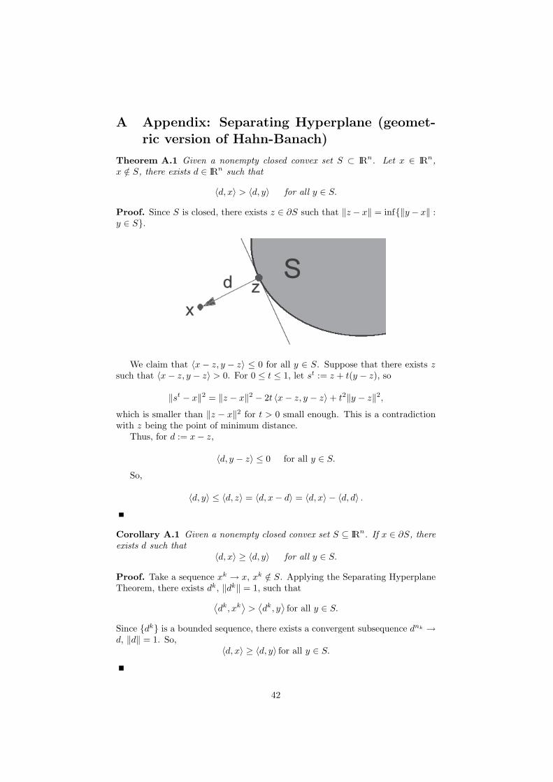
A Appendix: Separating Hyperplane (geomet-ric version of Hahn-Banach)

Theorem A.1 Given a nonempty closed convex set S ⊂ IRn. Let x ∈ IRn,x /∈ S, there exists d ∈ IRn such that

〈d, x〉 > 〈d, y〉 for all y ∈ S.

Proof. Since S is closed, there exists z ∈ ∂S such that ‖z − x‖ = inf{‖y − x‖ :y ∈ S}.

We claim that 〈x− z, y − z〉 ≤ 0 for all y ∈ S. Suppose that there exists zsuch that 〈x− z, y − z〉 > 0. For 0 ≤ t ≤ 1, let st := z + t(y − z), so

‖st − x‖2 = ‖z − x‖2 − 2t 〈x− z, y − z〉+ t2‖y − z‖2,which is smaller than ‖z − x‖2 for t > 0 small enough. This is a contradictionwith z being the point of minimum distance.

Thus, for d := x− z,

〈d, y − z〉 ≤ 0 for all y ∈ S.

So,

〈d, y〉 ≤ 〈d, z〉 = 〈d, x− d〉 = 〈d, x〉 − 〈d, d〉 .

Corollary A.1 Given a nonempty closed convex set S ⊆ IRn. If x ∈ ∂S, thereexists d such that

〈d, x〉 ≥ 〈d, y〉 for all y ∈ S.

Proof. Take a sequence xk → x, xk /∈ S. Applying the Separating HyperplaneTheorem, there exists dk, ‖dk‖ = 1, such that

⟨dk, xk

⟩>

⟨dk, y

⟩for all y ∈ S.

Since {dk} is a bounded sequence, there exists a convergent subsequence dnk →d, ‖d‖ = 1. So,

〈d, x〉 ≥ 〈d, y〉 for all y ∈ S.

42

B Appendix: Hahn-Banach for real vector spaces

Theorem B.1 (Hahn-Banach for real vector spaces). Let X be a Banachspace and p a convex functional on X, then there exists a linear functional λ onX such that

p(x) ≥ λ(x) ∀x ∈ X

Proof. Take 0 ∈ X, and define X = {0}, λ(0) = p(0).If ∃z ∈ X, z /∈ X, extend λ from X to the subspace generated by X and z,

λ(tz + x) = tλ(z) + λ(x).

Suppose x1, x2 ∈ X and α > 0, β > 0.

βλ(x1) + αλ(x2) = λ(βx1 + αx2)= (α + β)λ

(β

α+β x1 + αα+β x2

)

≤ (α + β)p(

βα+β x1 + α

α+β x2

)

= (α + β)p([

βα+β

](x1 − αz) +

[α

α+β

](x2 + βz)

)

≤ βp(x1 − αz) + αp(x2 + βz)

Thus,

β [−p(x1 − αz) + λ(x1)] ≤ α [p(x2 + βz)− λ(x2)]

1α

[−p(x1 − αz) + λ(x1)] ≤ 1β

[p(x2 + βz)− λ(x2)]

supx1∈X,α>0

1α

[−p(x1 − αz) + λ(x1)] ≤ a ≤ infx2∈X,β>0

1β

[p(x2 + βz)− λ(x2)]

Define λ(z) = a, then assuming t > 0,

λ(tz + x) = tλ(z) + λ(x) = ta + λ(tx)≤ t

(1t p(x + tz)− λ(x)

t

)+ λ(x)

≤ p(tz + x)

the case of t < 0 is similar. To extend for X, we will use the Zorn’s lemma.Let E be a collection of all extensions e of λ, e(x) ≤ p(x) for all x ∈ Xe. Wheree1 ≺ e2 if Xe1 ⊆ Xe2 and e1(x) = e2(x) in Xe1 . Thus, E is a partially orderedand E 6= ∅.

If {es}s∈J is a totally ordered subset of E , Λ = ∪s∈JXes is a subspace (monotoneunion of subspaces) and

e : Λ → IR, e(x) = es(x), if x ∈ Xes .

e is well defined and es ≺ e for all s ∈ J . Then e is maximal for J . Thus, Emust have a maximal element (Zorn’s Lemma) λ.

So, λ must be defined on X, otherwise we could extend it contradicting thefact that it is maximal.

43

References

[1] A. Belloni and A. Lucena, Improving on the Held and Karp Bound,Working Paper.

[2] A. Belloni and A. Lucena, Lagrangian Heuristics to Linear Ordering,Metaheuristics: Computer-Decision Making, Kluwer Academic Publishers,2004 (Book).

[3] A. Belloni and C. Sagastizabal, Dynamic Bundle Methods: Applica-tion to Combinatorial Optimization, Submitted to Mathematical Program-ming (July 2004).

[4] A. Belloni and R. Freund, Symmetry Points of a Convex Set: Ba-sic Properties and Computational Complexity, Submitted to MathematicalProgramming (July 2004).

[5] J. F. Bonnans, J. Ch. Gilbert, C. Lemarechal, and C. Sagas-tizabal,Numerical Optimization: Theoretical and Practical Aspects, Uni-versitext, Springer-Verlag, Berlin, 2003, xiv+423.

[6] A. Frangioni, Solving Semidefinite Quadratic Problems Within Nons-mooth Optimization Algorithms, Computers & Operations Research 23(11),p.1099 - 1118, 1996.

[7] M. Grotschel, M. Junger, and G. Reinelt, A cutting-plane algorithmfor the linear ordering problem,Operations Research, 32:1195-1220, 1984.

[8] M. Held and R. M. Karp, The traveling-salesman problem and minimumspaning tress, Operations Research, 17, 1138-1162, 1970.

[9] C. Helmberg and F. Rendl, A Spectral Bundle Method for SemidefiniteProgramming, SIAM J. Otimization, Vol. 10, No. 3, pp. 673-696.

[10] J.-B. Hiriart-Urruty and C. Lemarechal, Convex Analysis and Min-imization Algorithms I & II, Grund. der math. Wiss, no. 305-306, Springer-Verlag, 1993.

[11] R. T. Rockafellar, Convex Analysis Princeton University Press, 1970.

[12] N. Shor, Minimization methods for non-differentiable functions,Springer-Verlag, Berlin, 1985.

44