lecture notes for chapters 8 &10 introduction to data...
TRANSCRIPT
Excerpts for Data Mining Anomaly Detection
Lecture Notes for Chapters 8 &10
Introduction to Data Mining by
Tan, Steinbach, Kumar
© Tan,Steinbach, Kumar Introduction to Data Mining 4/18/2004 1
© Tan,Steinbach, Kumar Introduction to Data Mining 4/18/2004 ‹#›
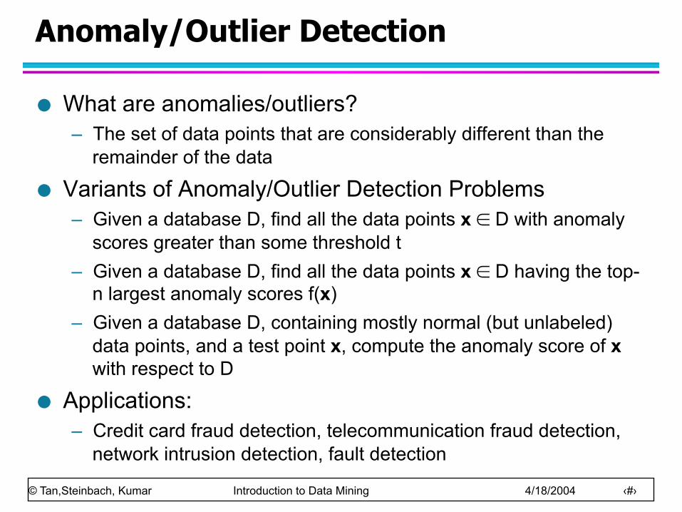
Anomaly/Outlier Detection
What are anomalies/outliers? – The set of data points that are considerably different than the
remainder of the data
Variants of Anomaly/Outlier Detection Problems – Given a database D, find all the data points x ∈ D with anomaly
scores greater than some threshold t – Given a database D, find all the data points x ∈ D having the top-
n largest anomaly scores f(x) – Given a database D, containing mostly normal (but unlabeled)
data points, and a test point x, compute the anomaly score of x with respect to D
Applications: – Credit card fraud detection, telecommunication fraud detection,
network intrusion detection, fault detection
© Tan,Steinbach, Kumar Introduction to Data Mining 4/18/2004 ‹#›
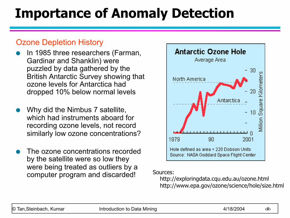
Importance of Anomaly Detection
Ozone Depletion History In 1985 three researchers (Farman,
Gardinar and Shanklin) were puzzled by data gathered by the British Antarctic Survey showing that ozone levels for Antarctica had dropped 10% below normal levels
Why did the Nimbus 7 satellite, which had instruments aboard for recording ozone levels, not record similarly low ozone concentrations?
The ozone concentrations recorded by the satellite were so low they were being treated as outliers by a computer program and discarded! Sources:
http://exploringdata.cqu.edu.au/ozone.html http://www.epa.gov/ozone/science/hole/size.html
© Tan,Steinbach, Kumar Introduction to Data Mining 4/18/2004 ‹#›
Anomaly Detection
Challenges – How many outliers are there in the data? – Method is unsupervised
u Validation can be quite challenging (just like for clustering)
– Finding needle in a haystack
Working assumption: – There are considerably more “normal” observations
than “abnormal” observations (outliers/anomalies) in the data
© Tan,Steinbach, Kumar Introduction to Data Mining 4/18/2004 ‹#›
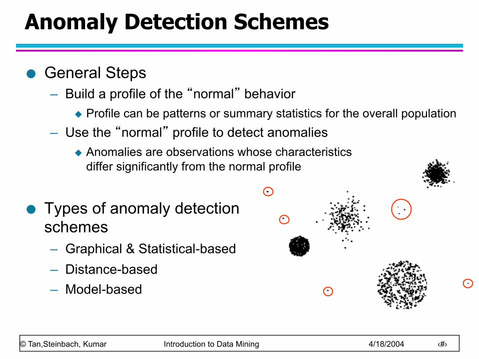
Anomaly Detection Schemes
General Steps – Build a profile of the “normal” behavior
u Profile can be patterns or summary statistics for the overall population – Use the “normal” profile to detect anomalies
u Anomalies are observations whose characteristics differ significantly from the normal profile
Types of anomaly detection schemes – Graphical & Statistical-based – Distance-based – Model-based
© Tan,Steinbach, Kumar Introduction to Data Mining 4/18/2004 ‹#›
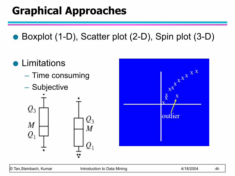
Graphical Approaches
Boxplot (1-D), Scatter plot (2-D), Spin plot (3-D)
Limitations – Time consuming – Subjective
© Tan,Steinbach, Kumar Introduction to Data Mining 4/18/2004 ‹#›
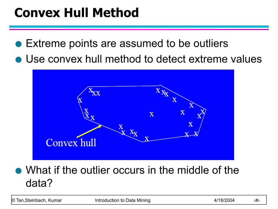
Convex Hull Method
Extreme points are assumed to be outliers Use convex hull method to detect extreme values
What if the outlier occurs in the middle of the data?
© Tan,Steinbach, Kumar Introduction to Data Mining 4/18/2004 ‹#›
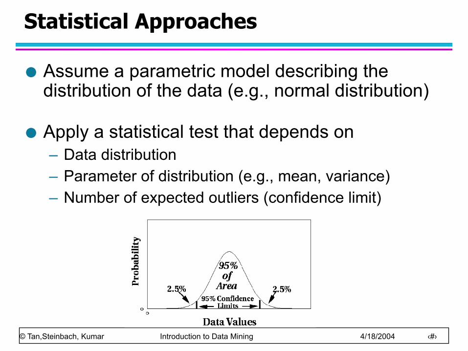
Statistical Approaches
Assume a parametric model describing the distribution of the data (e.g., normal distribution)
Apply a statistical test that depends on – Data distribution – Parameter of distribution (e.g., mean, variance) – Number of expected outliers (confidence limit)
© Tan,Steinbach, Kumar Introduction to Data Mining 4/18/2004 ‹#›
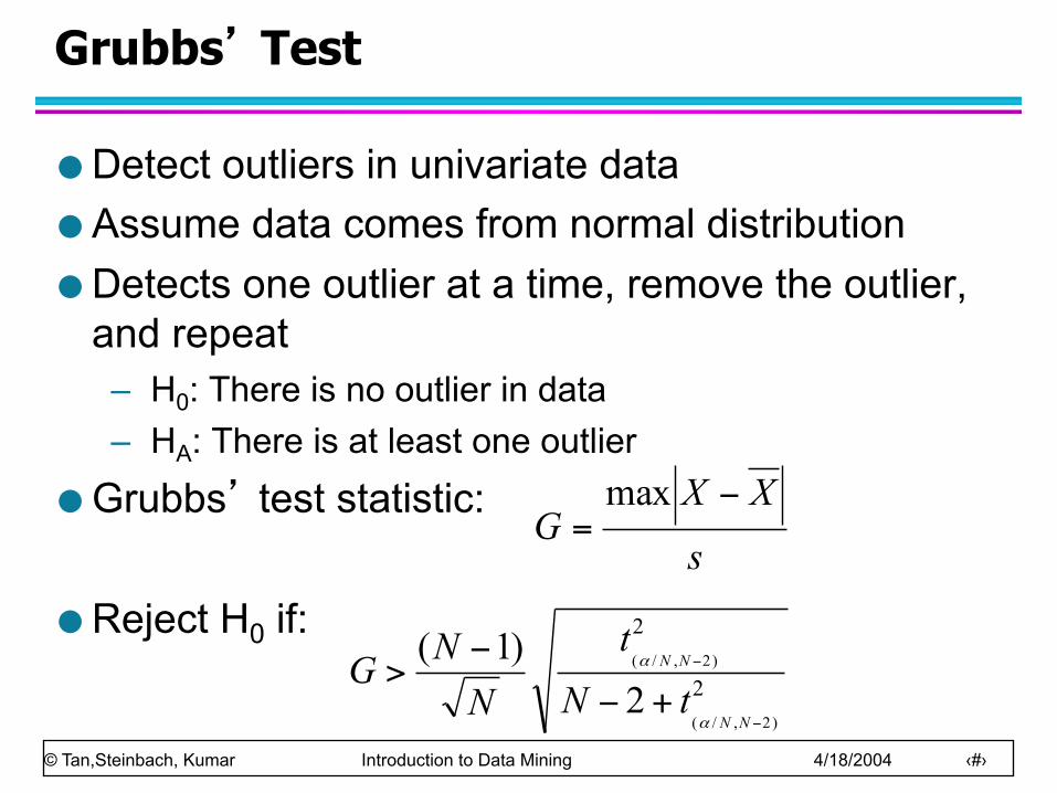
Grubbs’ Test
Detect outliers in univariate data Assume data comes from normal distribution Detects one outlier at a time, remove the outlier,
and repeat – H0: There is no outlier in data – HA: There is at least one outlier
Grubbs’ test statistic:
Reject H0 if: s
XXG
−=max
2
2
)2,/(
)2,/(
2)1(
−
−
+−−
>NN
NN
tNt
NNG
α
α
© Tan,Steinbach, Kumar Introduction to Data Mining 4/18/2004 ‹#›
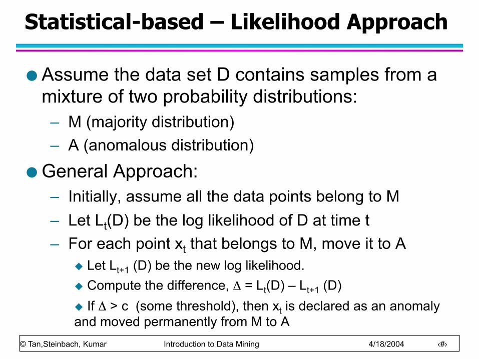
Statistical-based – Likelihood Approach
Assume the data set D contains samples from a mixture of two probability distributions: – M (majority distribution) – A (anomalous distribution)
General Approach: – Initially, assume all the data points belong to M – Let Lt(D) be the log likelihood of D at time t – For each point xt that belongs to M, move it to A
u Let Lt+1 (D) be the new log likelihood. u Compute the difference, Δ = Lt(D) – Lt+1 (D) u If Δ > c (some threshold), then xt is declared as an anomaly and moved permanently from M to A
© Tan,Steinbach, Kumar Introduction to Data Mining 4/18/2004 ‹#›
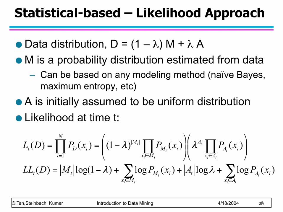
Statistical-based – Likelihood Approach
Data distribution, D = (1 – λ) M + λ A M is a probability distribution estimated from data
– Can be based on any modeling method (naïve Bayes, maximum entropy, etc)
A is initially assumed to be uniform distribution Likelihood at time t:
∑∑
∏∏∏
∈∈
∈∈=
+++−=
⎟⎟⎠
⎞⎜⎜⎝
⎛⎟⎟⎠
⎞⎜⎜⎝
⎛−==
ti
t
ti
t
ti
t
t
ti
t
t
AxiAt
MxiMtt
AxiA
A
MxiM
MN
iiDt
xPAxPMDLL
xPxPxPDL
)(loglog)(log)1log()(
)()()1()()( ||||
1
λλ
λλ
© Tan,Steinbach, Kumar Introduction to Data Mining 4/18/2004 ‹#›
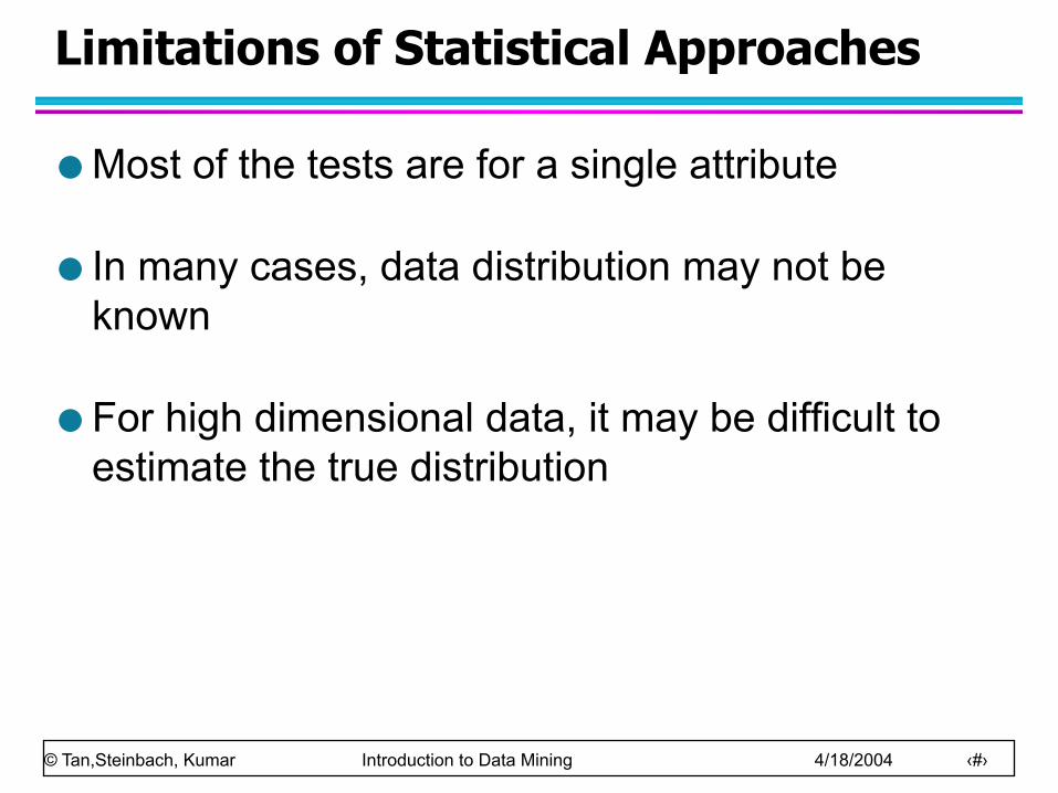
Limitations of Statistical Approaches
Most of the tests are for a single attribute
In many cases, data distribution may not be known
For high dimensional data, it may be difficult to estimate the true distribution
© Tan,Steinbach, Kumar Introduction to Data Mining 4/18/2004 ‹#›
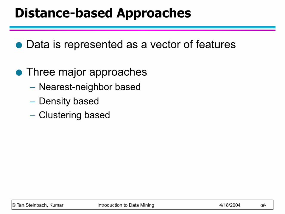
Distance-based Approaches
Data is represented as a vector of features
Three major approaches – Nearest-neighbor based – Density based – Clustering based
© Tan,Steinbach, Kumar Introduction to Data Mining 4/18/2004 ‹#›
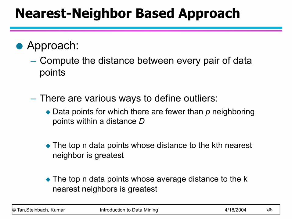
Nearest-Neighbor Based Approach
Approach: – Compute the distance between every pair of data
points
– There are various ways to define outliers: u Data points for which there are fewer than p neighboring
points within a distance D
u The top n data points whose distance to the kth nearest neighbor is greatest
u The top n data points whose average distance to the k nearest neighbors is greatest
© Tan,Steinbach, Kumar Introduction to Data Mining 4/18/2004 ‹#›
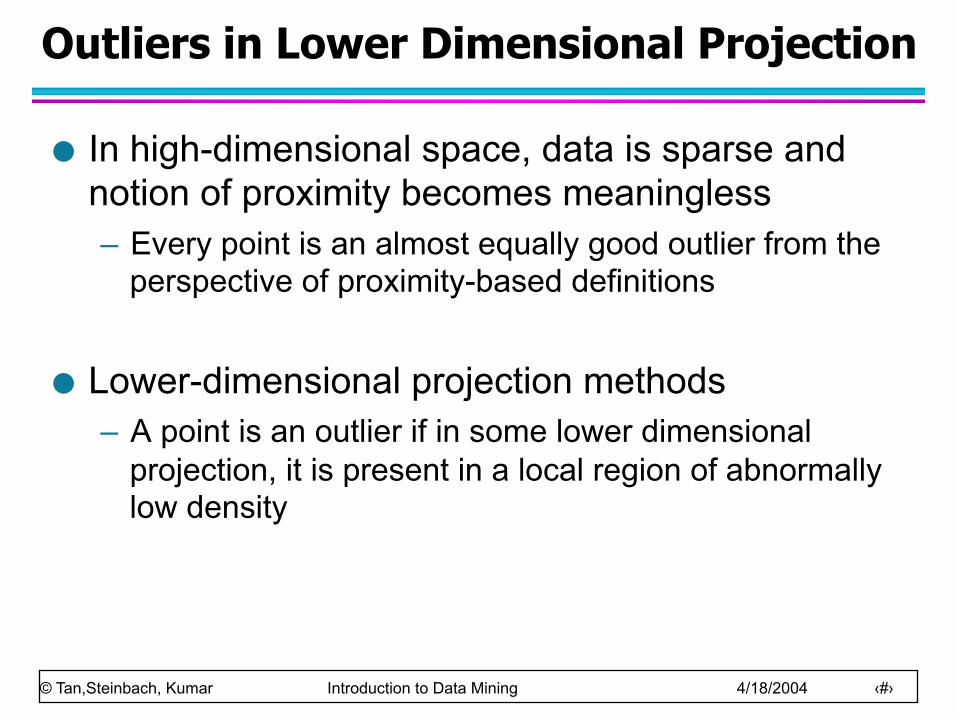
Outliers in Lower Dimensional Projection
In high-dimensional space, data is sparse and notion of proximity becomes meaningless – Every point is an almost equally good outlier from the
perspective of proximity-based definitions
Lower-dimensional projection methods – A point is an outlier if in some lower dimensional
projection, it is present in a local region of abnormally low density
© Tan,Steinbach, Kumar Introduction to Data Mining 4/18/2004 ‹#›
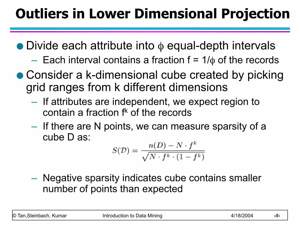
Outliers in Lower Dimensional Projection
Divide each attribute into φ equal-depth intervals – Each interval contains a fraction f = 1/φ of the records
Consider a k-dimensional cube created by picking grid ranges from k different dimensions – If attributes are independent, we expect region to
contain a fraction fk of the records – If there are N points, we can measure sparsity of a
cube D as:
– Negative sparsity indicates cube contains smaller number of points than expected
© Tan,Steinbach, Kumar Introduction to Data Mining 4/18/2004 ‹#›
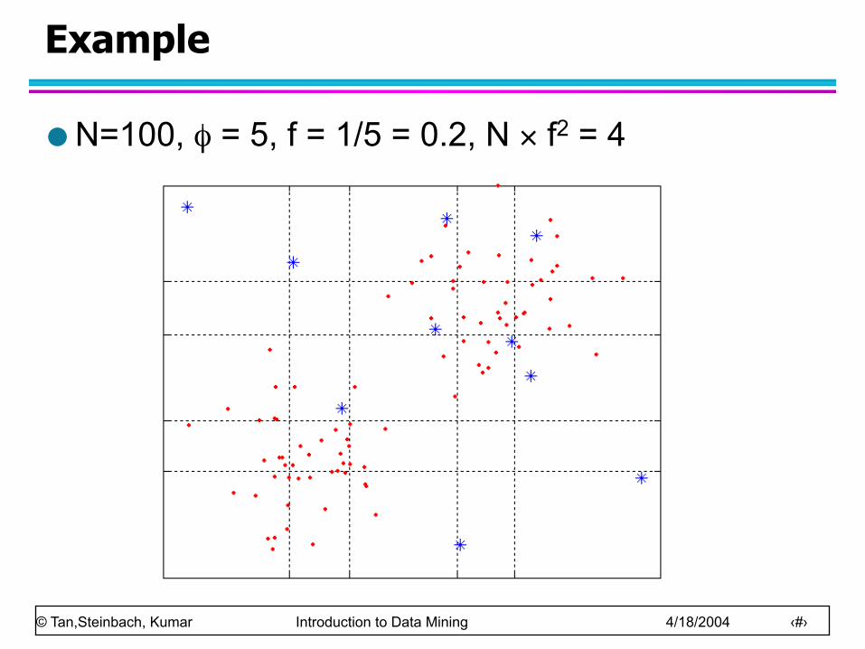
Example
N=100, φ = 5, f = 1/5 = 0.2, N × f2 = 4
© Tan,Steinbach, Kumar Introduction to Data Mining 4/18/2004 ‹#›
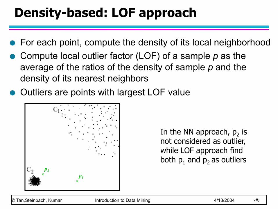
Density-based: LOF approach
For each point, compute the density of its local neighborhood Compute local outlier factor (LOF) of a sample p as the
average of the ratios of the density of sample p and the density of its nearest neighbors
Outliers are points with largest LOF value
p2 × p1
×
In the NN approach, p2 is not considered as outlier, while LOF approach find both p1 and p2 as outliers
© Tan,Steinbach, Kumar Introduction to Data Mining 4/18/2004 ‹#›
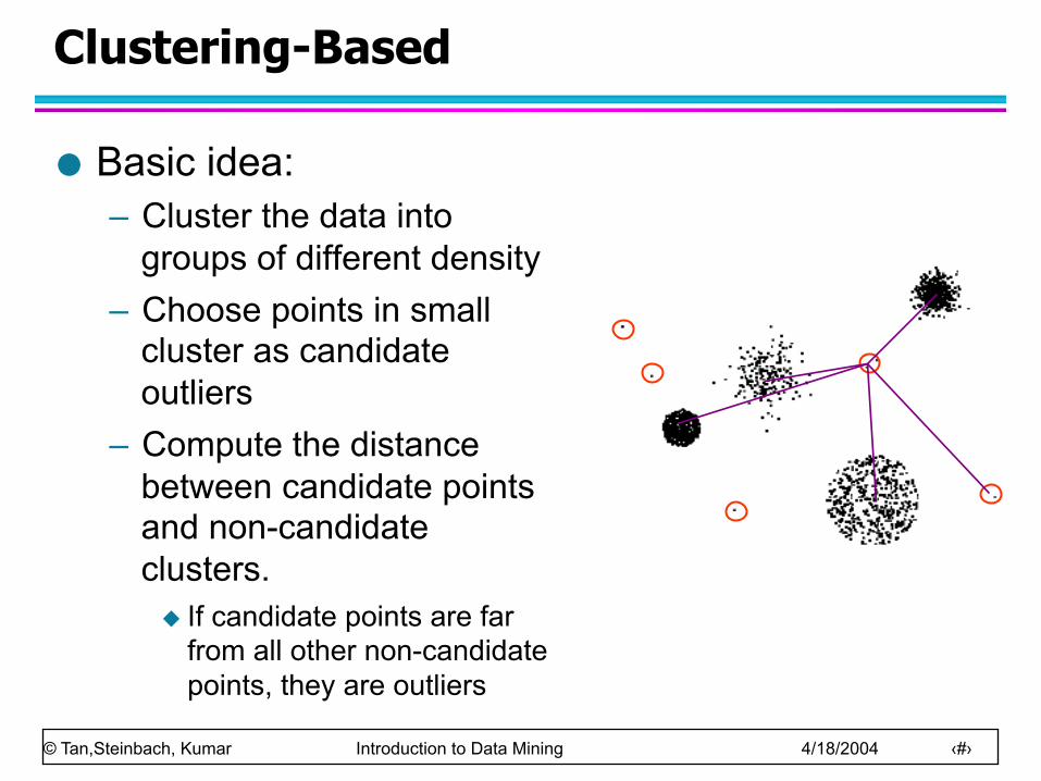
Clustering-Based
Basic idea: – Cluster the data into
groups of different density – Choose points in small
cluster as candidate outliers
– Compute the distance between candidate points and non-candidate clusters.
u If candidate points are far from all other non-candidate points, they are outliers
© Tan,Steinbach, Kumar Introduction to Data Mining 4/18/2004 ‹#›
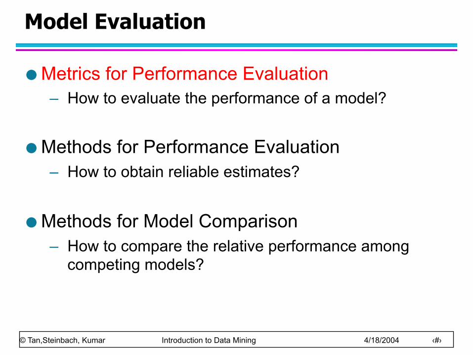
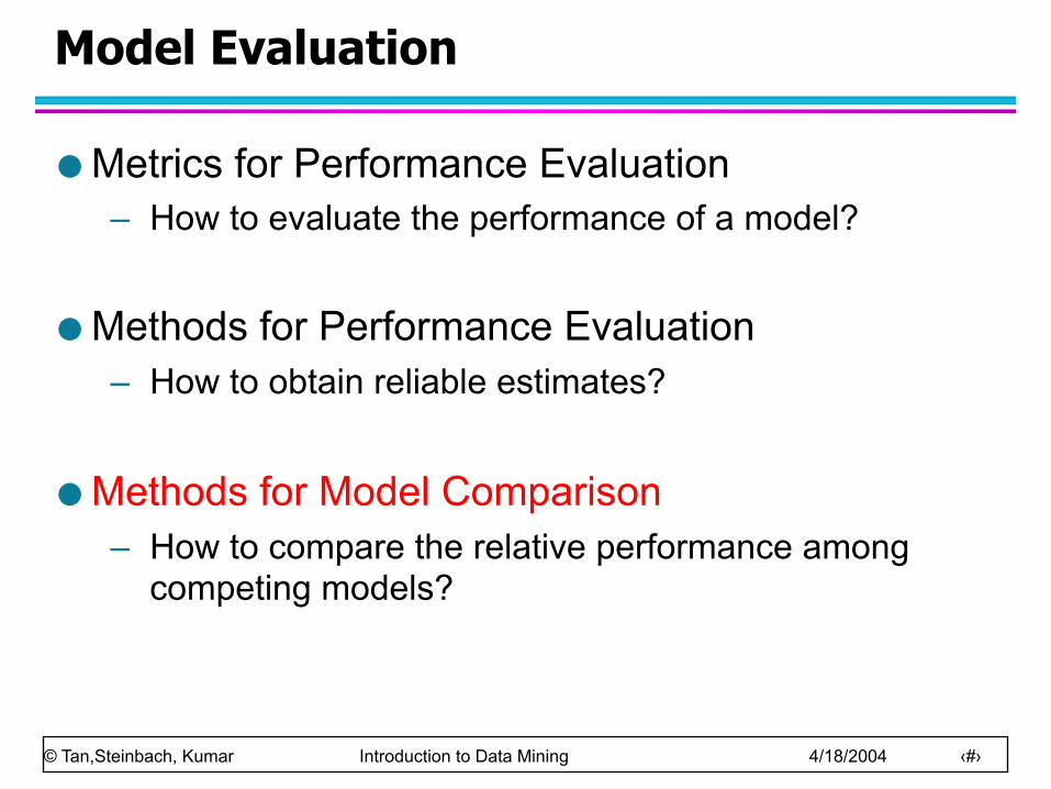
Model Evaluation
Metrics for Performance Evaluation – How to evaluate the performance of a model?
Methods for Performance Evaluation – How to obtain reliable estimates?
Methods for Model Comparison – How to compare the relative performance among
competing models?
© Tan,Steinbach, Kumar Introduction to Data Mining 4/18/2004 ‹#›
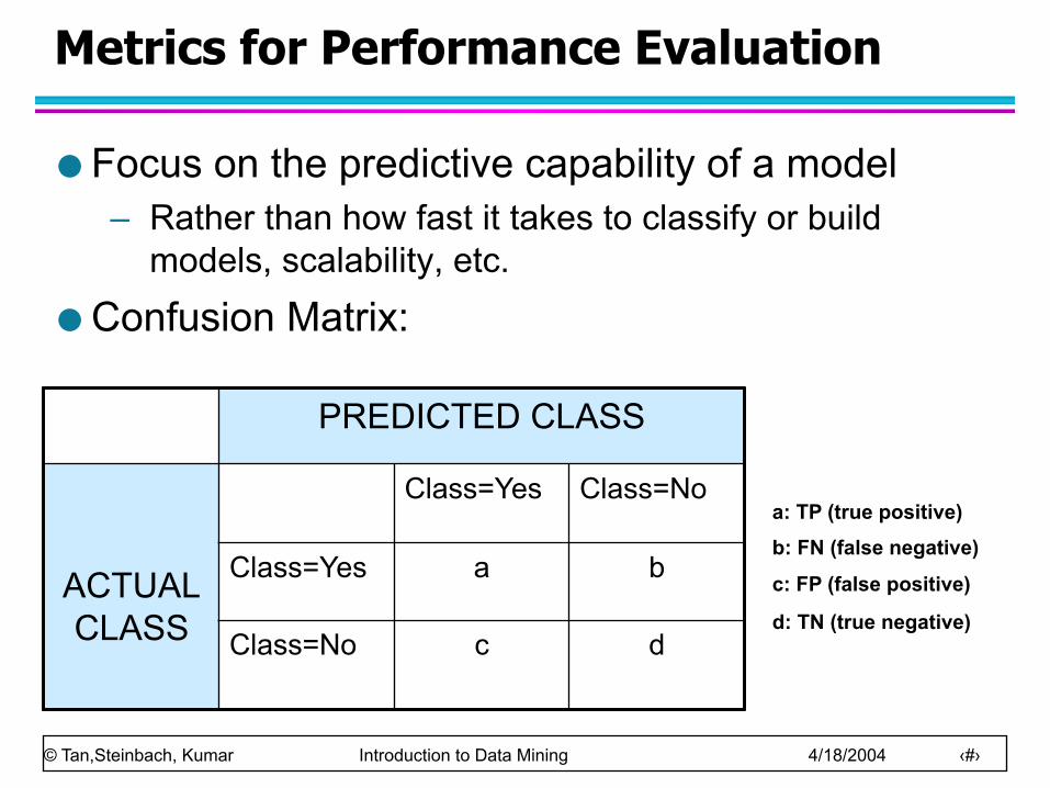
Metrics for Performance Evaluation
Focus on the predictive capability of a model – Rather than how fast it takes to classify or build
models, scalability, etc.
Confusion Matrix:
PREDICTED CLASS
ACTUAL CLASS
Class=Yes Class=No
Class=Yes a b
Class=No c d
a: TP (true positive)
b: FN (false negative)
c: FP (false positive)
d: TN (true negative)
© Tan,Steinbach, Kumar Introduction to Data Mining 4/18/2004 ‹#›
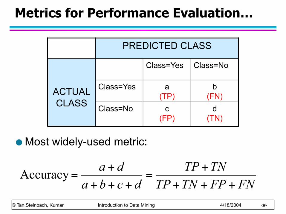
Metrics for Performance Evaluation…
Most widely-used metric:
PREDICTED CLASS
ACTUAL CLASS
Class=Yes Class=No
Class=Yes a (TP)
b (FN)
Class=No c (FP)
d (TN)
FNFPTNTPTNTP
dcbada
++++
=+++
+=Accuracy
© Tan,Steinbach, Kumar Introduction to Data Mining 4/18/2004 ‹#›
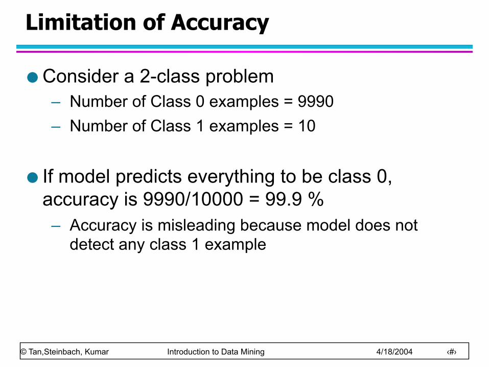
Limitation of Accuracy
Consider a 2-class problem – Number of Class 0 examples = 9990 – Number of Class 1 examples = 10
If model predicts everything to be class 0, accuracy is 9990/10000 = 99.9 % – Accuracy is misleading because model does not
detect any class 1 example
© Tan,Steinbach, Kumar Introduction to Data Mining 4/18/2004 ‹#›
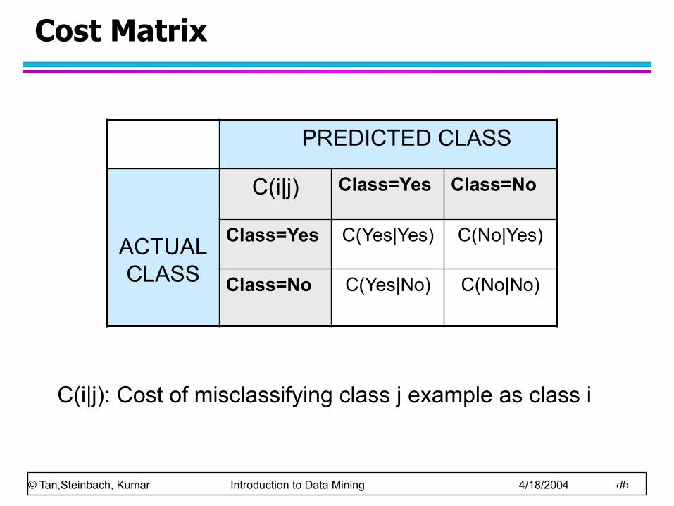
Cost Matrix
PREDICTED CLASS
ACTUAL CLASS
C(i|j) Class=Yes Class=No
Class=Yes C(Yes|Yes) C(No|Yes)
Class=No C(Yes|No) C(No|No)
C(i|j): Cost of misclassifying class j example as class i
© Tan,Steinbach, Kumar Introduction to Data Mining 4/18/2004 ‹#›
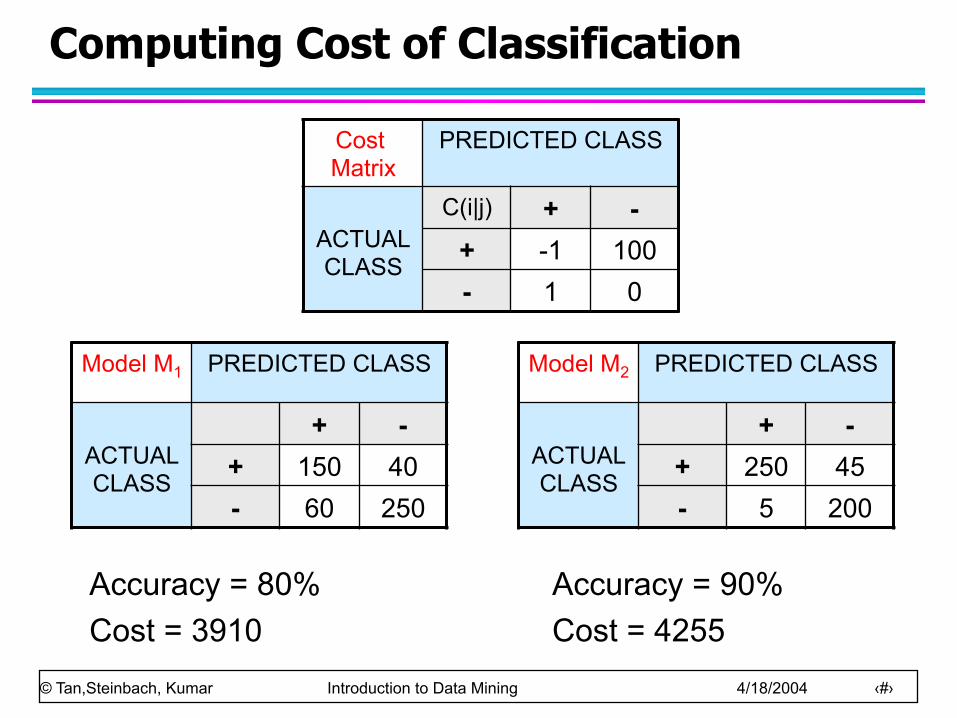
Computing Cost of Classification
Cost Matrix
PREDICTED CLASS
ACTUAL CLASS
C(i|j) + - + -1 100 - 1 0
Model M1 PREDICTED CLASS
ACTUAL CLASS
+ - + 150 40 - 60 250
Model M2 PREDICTED CLASS
ACTUAL CLASS
+ - + 250 45 - 5 200
Accuracy = 80% Cost = 3910
Accuracy = 90% Cost = 4255
© Tan,Steinbach, Kumar Introduction to Data Mining 4/18/2004 ‹#›
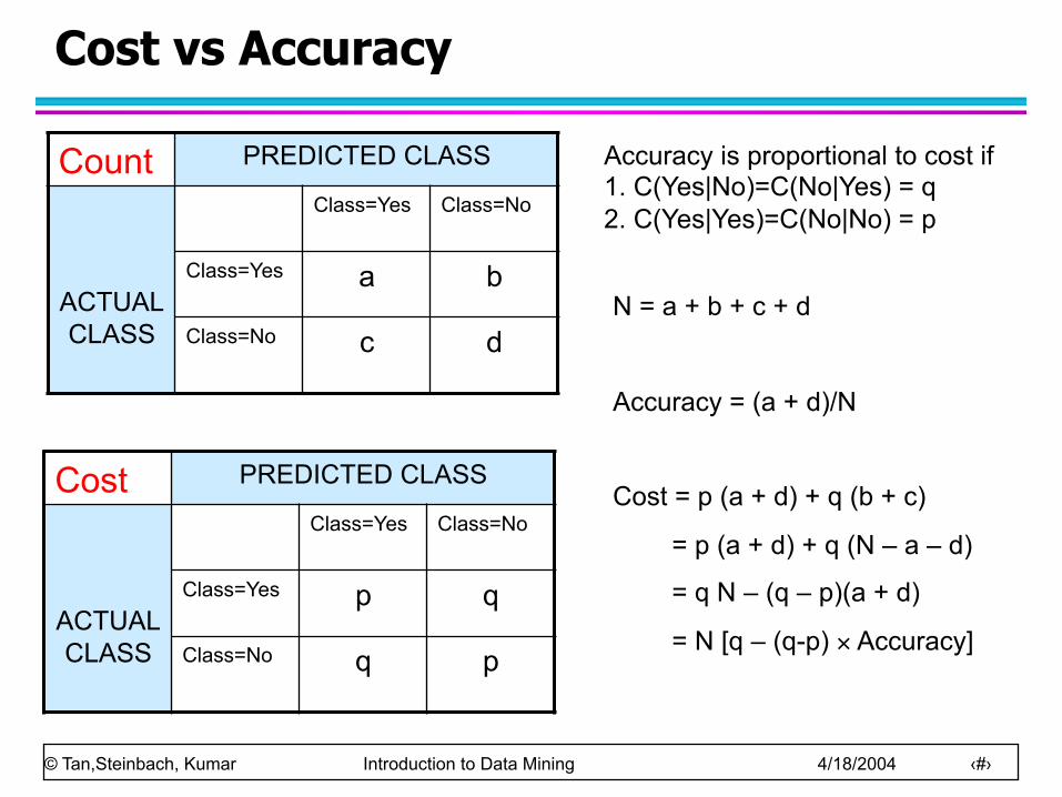
Cost vs Accuracy
Count PREDICTED CLASS
ACTUAL CLASS
Class=Yes Class=No
Class=Yes a b
Class=No c d
Cost PREDICTED CLASS
ACTUAL CLASS
Class=Yes Class=No
Class=Yes p q
Class=No q p
N = a + b + c + d
Accuracy = (a + d)/N
Cost = p (a + d) + q (b + c)
= p (a + d) + q (N – a – d)
= q N – (q – p)(a + d)
= N [q – (q-p) × Accuracy]
Accuracy is proportional to cost if 1. C(Yes|No)=C(No|Yes) = q 2. C(Yes|Yes)=C(No|No) = p
© Tan,Steinbach, Kumar Introduction to Data Mining 4/18/2004 ‹#›
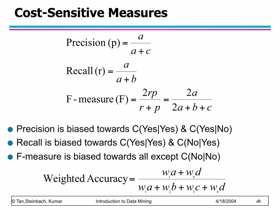
Cost-Sensitive Measures
cbaa
prrp
baa
caa
++=
+=
+=
+=
222(F) measure-F
(r) Recall
(p)Precision
Precision is biased towards C(Yes|Yes) & C(Yes|No) Recall is biased towards C(Yes|Yes) & C(No|Yes) F-measure is biased towards all except C(No|No)
dwcwbwawdwaw
4321
41Accuracy Weighted+++
+=
© Tan,Steinbach, Kumar Introduction to Data Mining 4/18/2004 ‹#›
Model Evaluation
Metrics for Performance Evaluation – How to evaluate the performance of a model?
Methods for Performance Evaluation – How to obtain reliable estimates?
Methods for Model Comparison – How to compare the relative performance among
competing models?
© Tan,Steinbach, Kumar Introduction to Data Mining 4/18/2004 ‹#›
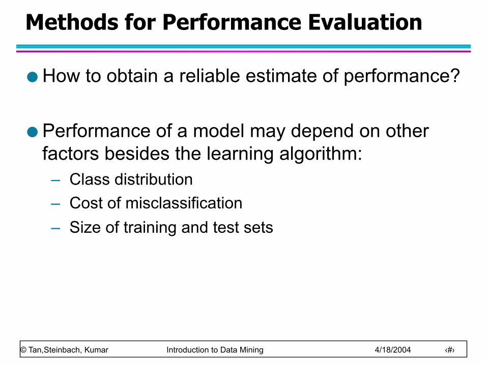
Methods for Performance Evaluation
How to obtain a reliable estimate of performance?
Performance of a model may depend on other factors besides the learning algorithm: – Class distribution – Cost of misclassification – Size of training and test sets
© Tan,Steinbach, Kumar Introduction to Data Mining 4/18/2004 ‹#›
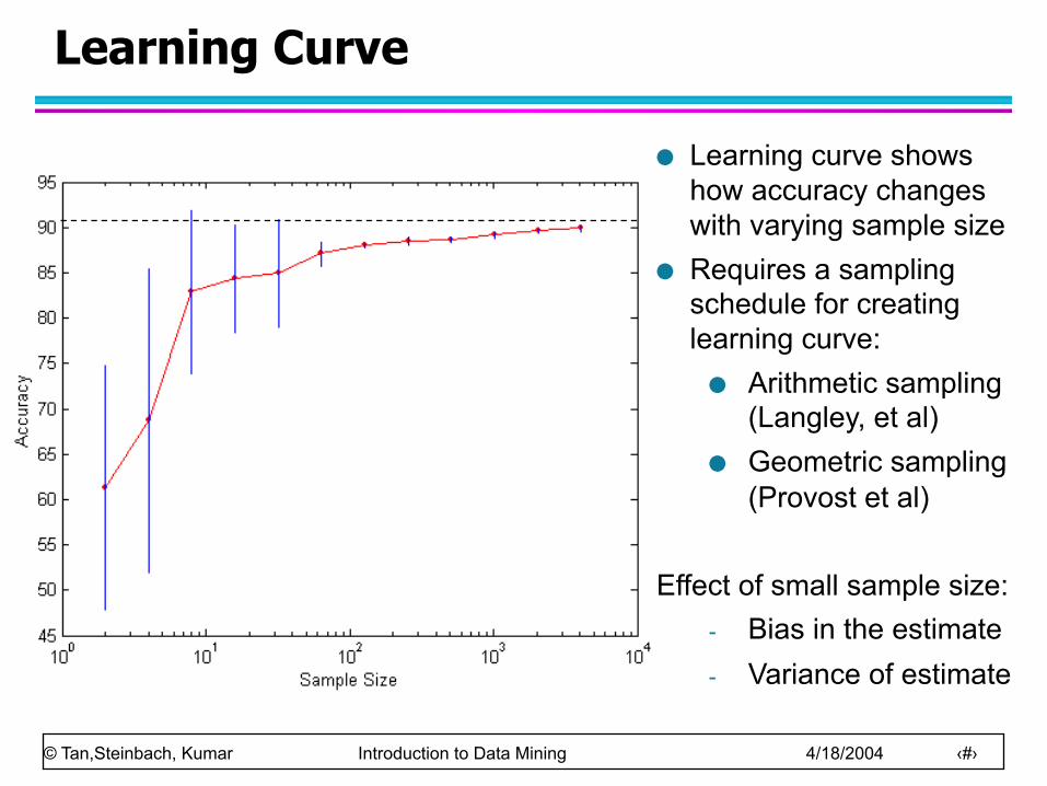
Learning Curve
Learning curve shows how accuracy changes with varying sample size
Requires a sampling schedule for creating learning curve: Arithmetic sampling
(Langley, et al) Geometric sampling
(Provost et al) Effect of small sample size:
- Bias in the estimate - Variance of estimate
© Tan,Steinbach, Kumar Introduction to Data Mining 4/18/2004 ‹#›
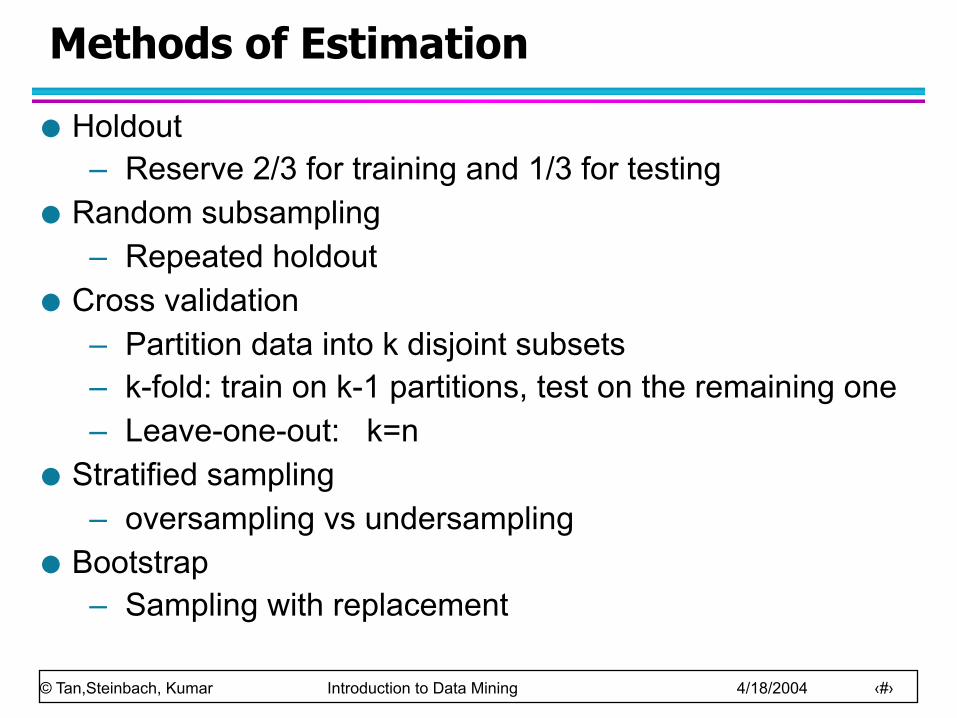
Methods of Estimation
Holdout – Reserve 2/3 for training and 1/3 for testing
Random subsampling – Repeated holdout
Cross validation – Partition data into k disjoint subsets – k-fold: train on k-1 partitions, test on the remaining one – Leave-one-out: k=n
Stratified sampling – oversampling vs undersampling
Bootstrap – Sampling with replacement
© Tan,Steinbach, Kumar Introduction to Data Mining 4/18/2004 ‹#›
Model Evaluation
Metrics for Performance Evaluation – How to evaluate the performance of a model?
Methods for Performance Evaluation – How to obtain reliable estimates?
Methods for Model Comparison – How to compare the relative performance among
competing models?
© Tan,Steinbach, Kumar Introduction to Data Mining 4/18/2004 ‹#›
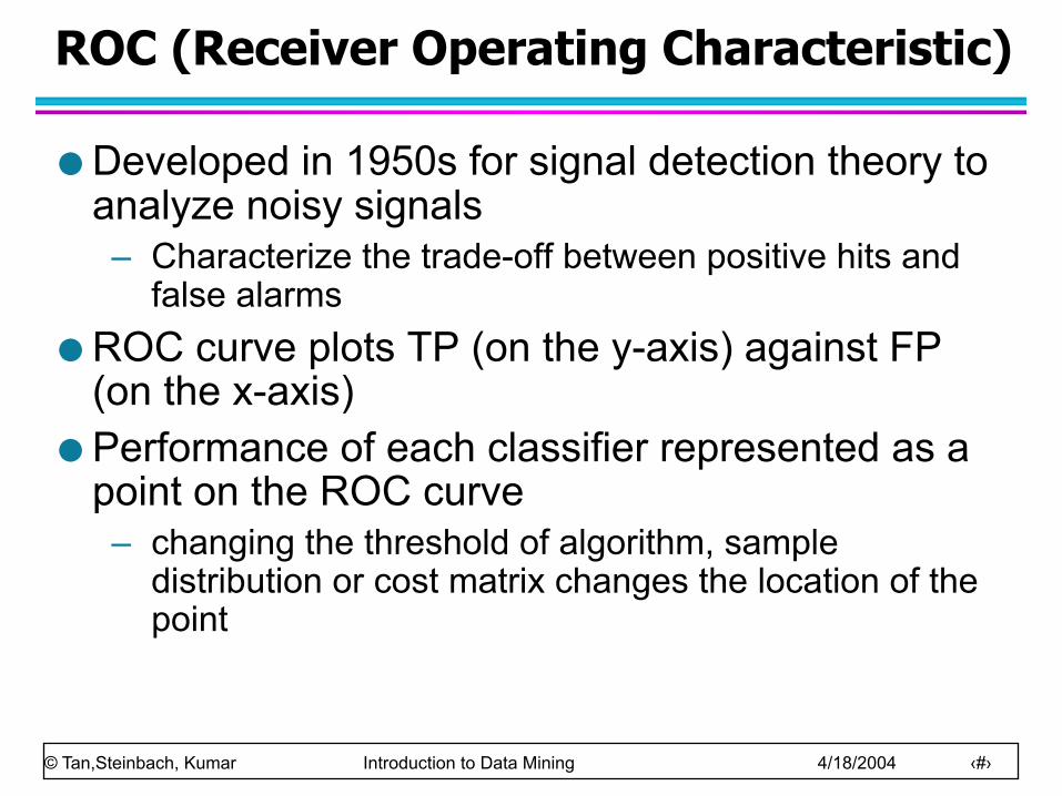
ROC (Receiver Operating Characteristic)
Developed in 1950s for signal detection theory to analyze noisy signals – Characterize the trade-off between positive hits and
false alarms ROC curve plots TP (on the y-axis) against FP
(on the x-axis) Performance of each classifier represented as a
point on the ROC curve – changing the threshold of algorithm, sample
distribution or cost matrix changes the location of the point
© Tan,Steinbach, Kumar Introduction to Data Mining 4/18/2004 ‹#›
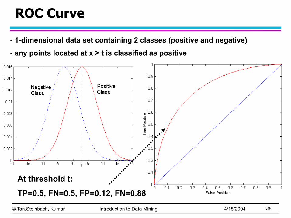
ROC Curve
At threshold t:
TP=0.5, FN=0.5, FP=0.12, FN=0.88
- 1-dimensional data set containing 2 classes (positive and negative)
- any points located at x > t is classified as positive
© Tan,Steinbach, Kumar Introduction to Data Mining 4/18/2004 ‹#›
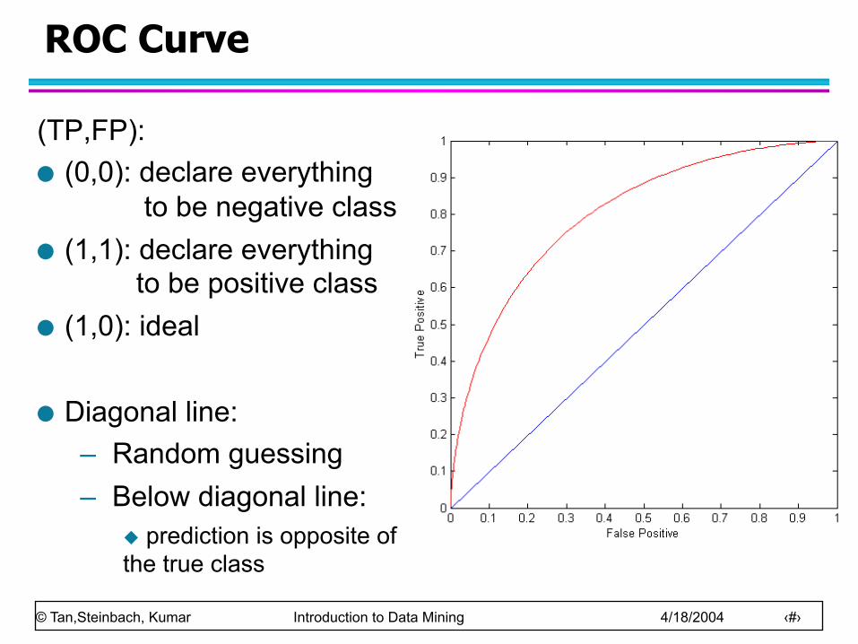
ROC Curve
(TP,FP): (0,0): declare everything
to be negative class (1,1): declare everything
to be positive class (1,0): ideal Diagonal line:
– Random guessing – Below diagonal line:
u prediction is opposite of the true class
© Tan,Steinbach, Kumar Introduction to Data Mining 4/18/2004 ‹#›
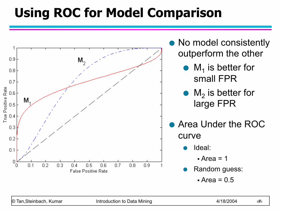
Using ROC for Model Comparison
No model consistently outperform the other M1 is better for
small FPR M2 is better for
large FPR
Area Under the ROC curve Ideal:
§ Area = 1 Random guess:
§ Area = 0.5
© Tan,Steinbach, Kumar Introduction to Data Mining 4/18/2004 ‹#›
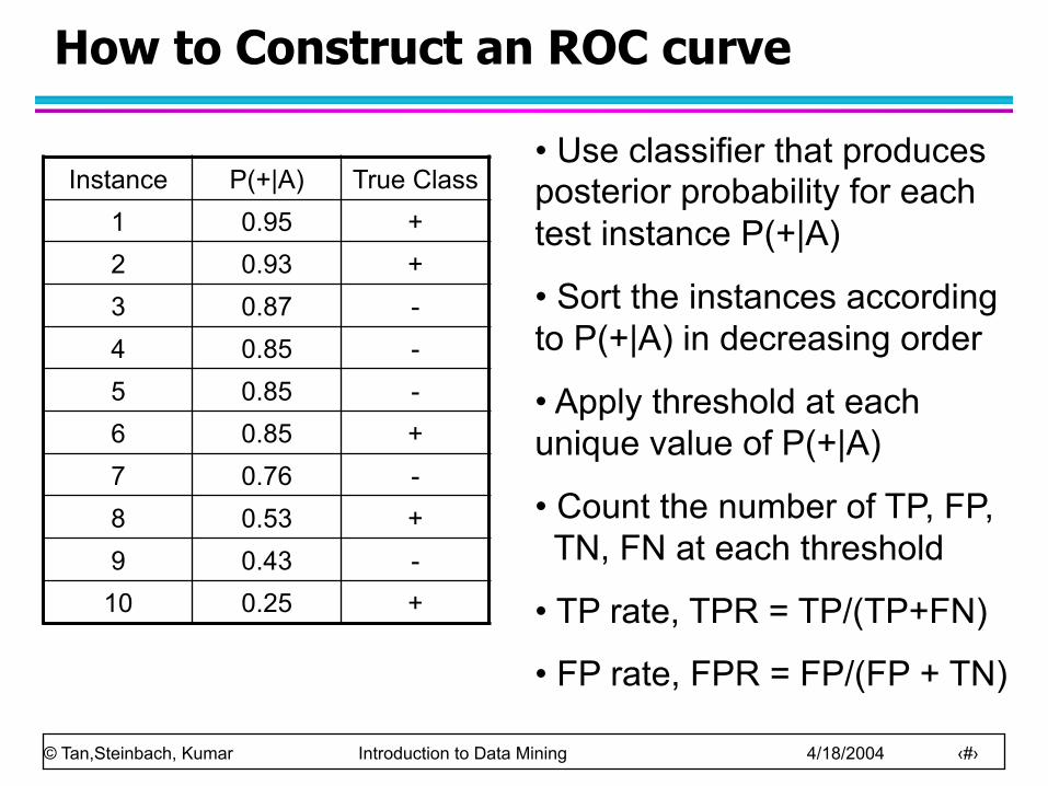
How to Construct an ROC curve
Instance P(+|A) True Class 1 0.95 + 2 0.93 + 3 0.87 - 4 0.85 - 5 0.85 - 6 0.85 + 7 0.76 - 8 0.53 + 9 0.43 -
10 0.25 +
• Use classifier that produces posterior probability for each test instance P(+|A)
• Sort the instances according to P(+|A) in decreasing order
• Apply threshold at each unique value of P(+|A)
• Count the number of TP, FP, TN, FN at each threshold
• TP rate, TPR = TP/(TP+FN)
• FP rate, FPR = FP/(FP + TN)
© Tan,Steinbach, Kumar Introduction to Data Mining 4/18/2004 ‹#›
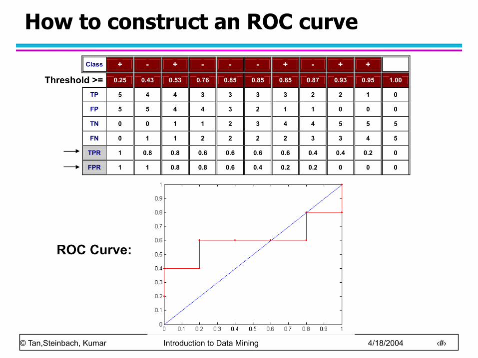
How to construct an ROC curve
Class + - + - - - + - + + P 0.25 0.43 0.53 0.76 0.85 0.85 0.85 0.87 0.93 0.95 1.00
TP 5 4 4 3 3 3 3 2 2 1 0
FP 5 5 4 4 3 2 1 1 0 0 0
TN 0 0 1 1 2 3 4 4 5 5 5
FN 0 1 1 2 2 2 2 3 3 4 5
TPR 1 0.8 0.8 0.6 0.6 0.6 0.6 0.4 0.4 0.2 0
FPR 1 1 0.8 0.8 0.6 0.4 0.2 0.2 0 0 0
Threshold >=
ROC Curve:
© Tan,Steinbach, Kumar Introduction to Data Mining 4/18/2004 ‹#›
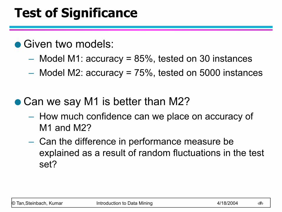
Test of Significance
Given two models: – Model M1: accuracy = 85%, tested on 30 instances – Model M2: accuracy = 75%, tested on 5000 instances
Can we say M1 is better than M2? – How much confidence can we place on accuracy of
M1 and M2? – Can the difference in performance measure be
explained as a result of random fluctuations in the test set?
© Tan,Steinbach, Kumar Introduction to Data Mining 4/18/2004 ‹#›
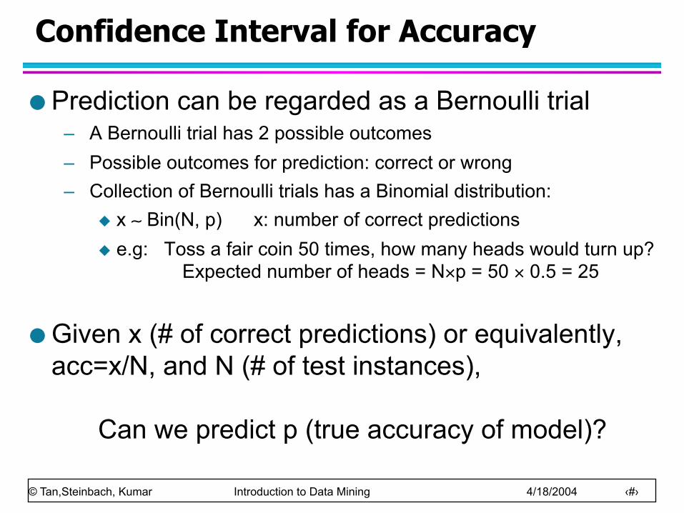
Confidence Interval for Accuracy
Prediction can be regarded as a Bernoulli trial – A Bernoulli trial has 2 possible outcomes – Possible outcomes for prediction: correct or wrong – Collection of Bernoulli trials has a Binomial distribution:
u x ∼ Bin(N, p) x: number of correct predictions u e.g: Toss a fair coin 50 times, how many heads would turn up? Expected number of heads = N×p = 50 × 0.5 = 25
Given x (# of correct predictions) or equivalently, acc=x/N, and N (# of test instances),
Can we predict p (true accuracy of model)?
© Tan,Steinbach, Kumar Introduction to Data Mining 4/18/2004 ‹#›
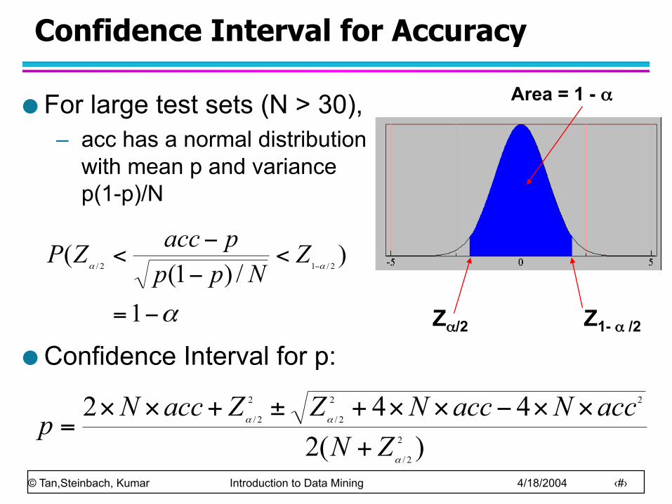
Confidence Interval for Accuracy
For large test sets (N > 30), – acc has a normal distribution
with mean p and variance p(1-p)/N
Confidence Interval for p:
α
αα
−=
<−−
<−
1
)/)1(
(2/12/
ZNpp
paccZP
Area = 1 - α
Zα/2 Z1- α /2
)(2442
2
2/
22
2/
2
2/
α
αα
ZNaccNaccNZZaccNp
+
××−××+±+××=
© Tan,Steinbach, Kumar Introduction to Data Mining 4/18/2004 ‹#›
Confidence Interval for Accuracy
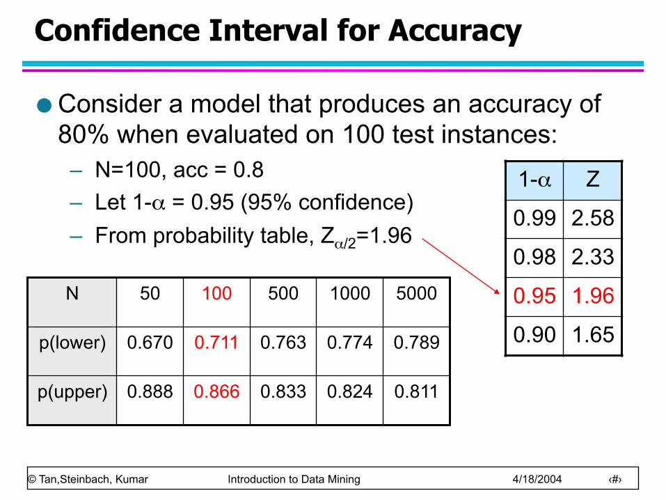
Consider a model that produces an accuracy of 80% when evaluated on 100 test instances: – N=100, acc = 0.8 – Let 1-α = 0.95 (95% confidence) – From probability table, Zα/2=1.96
1-α Z
0.99 2.58
0.98 2.33
0.95 1.96
0.90 1.65
N 50 100 500 1000 5000
p(lower) 0.670 0.711 0.763 0.774 0.789
p(upper) 0.888 0.866 0.833 0.824 0.811
© Tan,Steinbach, Kumar Introduction to Data Mining 4/18/2004 ‹#›
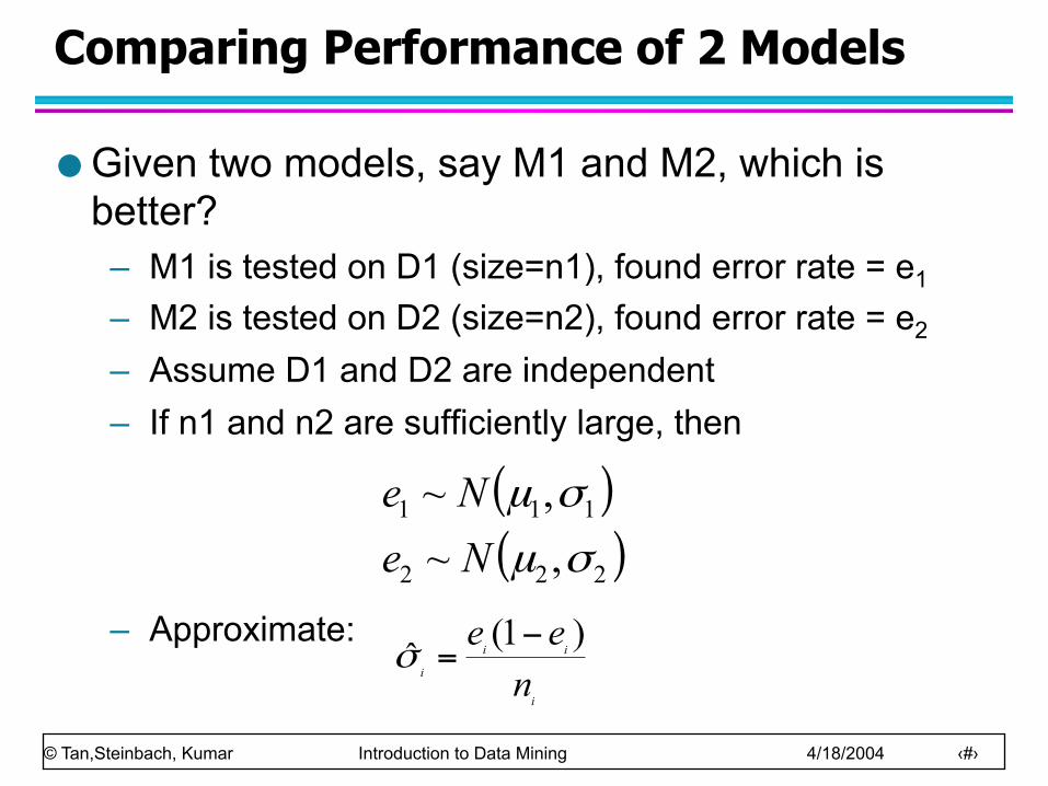
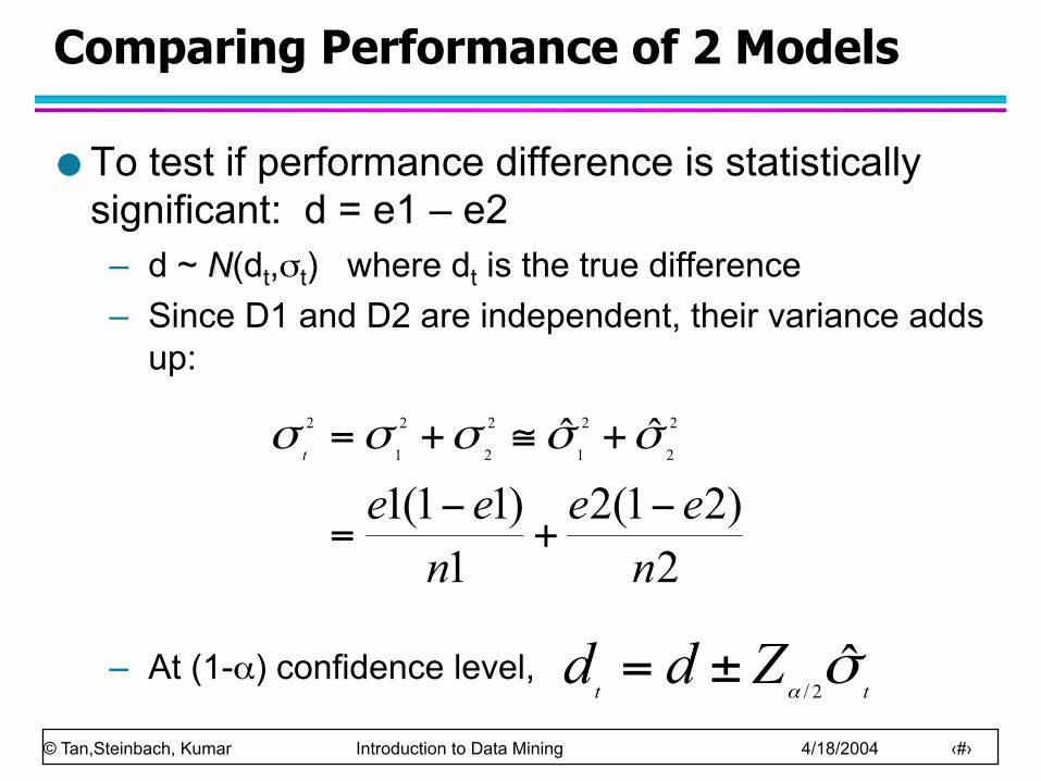
Comparing Performance of 2 Models
Given two models, say M1 and M2, which is better? – M1 is tested on D1 (size=n1), found error rate = e1
– M2 is tested on D2 (size=n2), found error rate = e2
– Assume D1 and D2 are independent – If n1 and n2 are sufficiently large, then
– Approximate:
( )( )222
111
,~,~σµ
σµ
NeNe
i
ii
i nee )1(ˆ −
=σ
© Tan,Steinbach, Kumar Introduction to Data Mining 4/18/2004 ‹#›
Comparing Performance of 2 Models
To test if performance difference is statistically significant: d = e1 – e2 – d ~ N(dt,σt) where dt is the true difference – Since D1 and D2 are independent, their variance adds
up:
– At (1-α) confidence level,
2)21(2
1)11(1
ˆˆ 2
2
2
1
2
2
2
1
2
nee
nee
t
−+
−=
+≅+= σσσσσ
ttZdd σ
αˆ
2/±=
© Tan,Steinbach, Kumar Introduction to Data Mining 4/18/2004 ‹#›
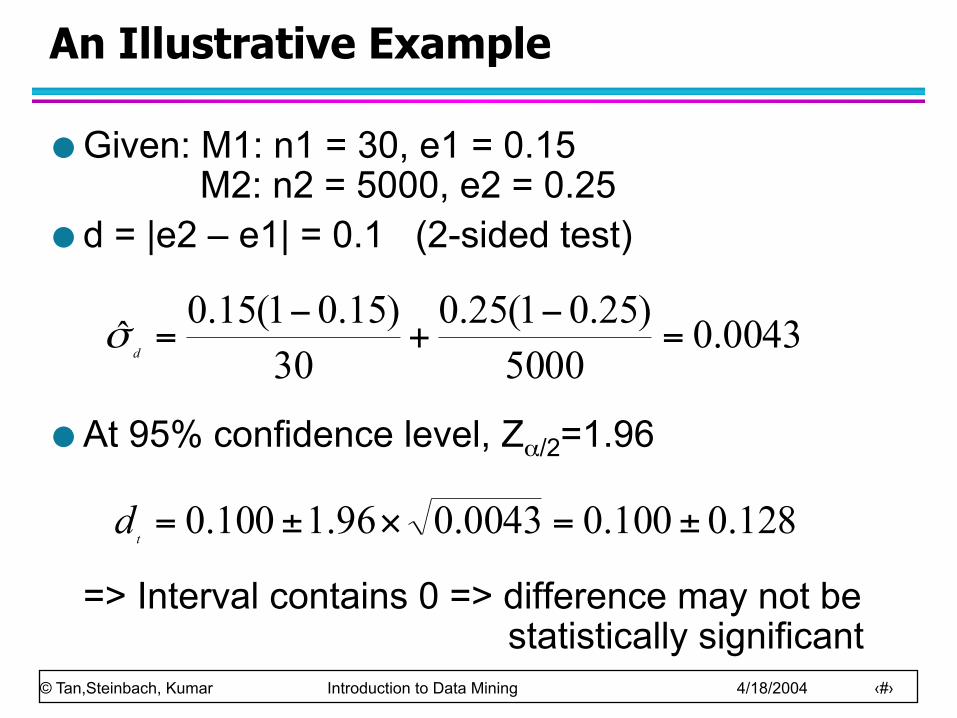
An Illustrative Example
Given: M1: n1 = 30, e1 = 0.15 M2: n2 = 5000, e2 = 0.25
d = |e2 – e1| = 0.1 (2-sided test)
At 95% confidence level, Zα/2=1.96
=> Interval contains 0 => difference may not be
statistically significant
0043.05000
)25.01(25.030
)15.01(15.0ˆ =−
+−
=d
σ
128.0100.00043.096.1100.0 ±=×±=td
© Tan,Steinbach, Kumar Introduction to Data Mining 4/18/2004 ‹#›
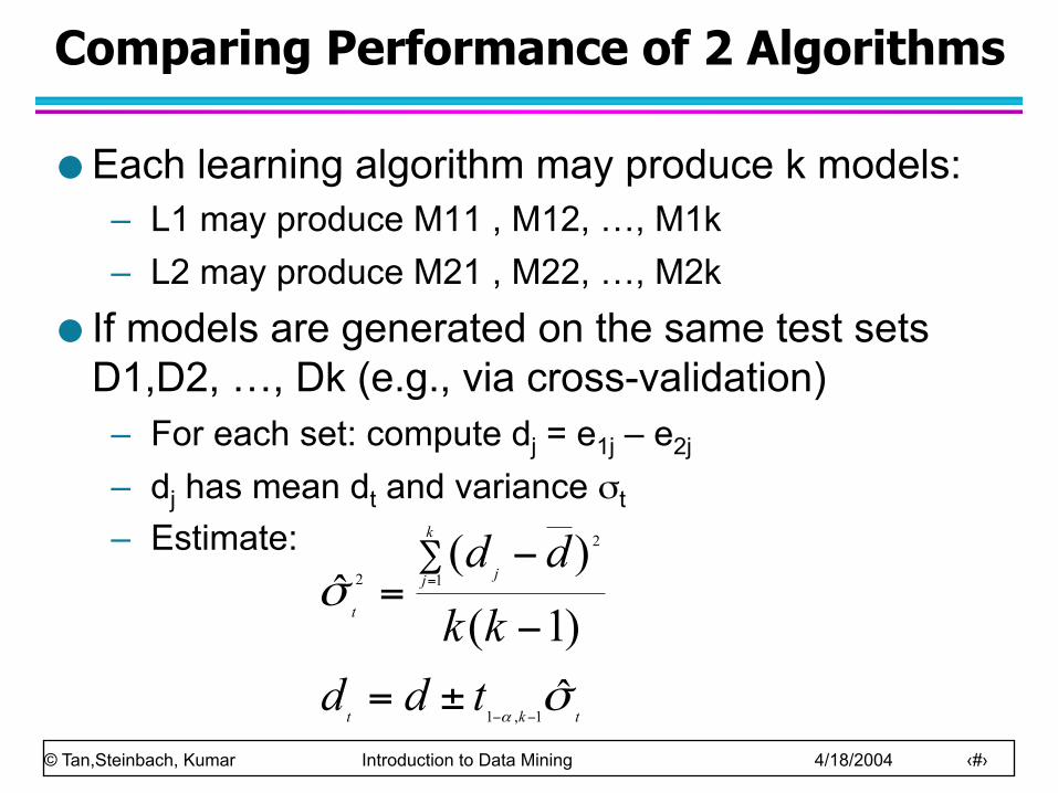
Comparing Performance of 2 Algorithms
Each learning algorithm may produce k models: – L1 may produce M11 , M12, …, M1k – L2 may produce M21 , M22, …, M2k
If models are generated on the same test sets D1,D2, …, Dk (e.g., via cross-validation) – For each set: compute dj = e1j – e2j
– dj has mean dt and variance σt – Estimate:
tkt
k
j j
t
tddkkdd
σ
σ
αˆ)1()(
ˆ
1,1
1
2
2
−−
=
±=
−
−=∑
© Tan,Steinbach, Kumar Introduction to Data Mining 4/18/2004 ‹#›
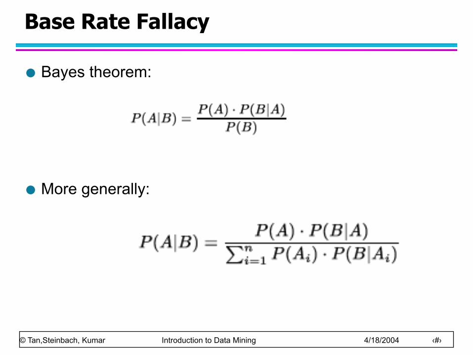
Base Rate Fallacy
Bayes theorem:
More generally:

© Tan,Steinbach, Kumar Introduction to Data Mining 4/18/2004 ‹#›
Base Rate Fallacy (Axelsson, 1999)

© Tan,Steinbach, Kumar Introduction to Data Mining 4/18/2004 ‹#›
Base Rate Fallacy
Even though the test is 99% certain, your chance of having the disease is 1/100, because the population of healthy people is much larger than sick people
© Tan,Steinbach, Kumar Introduction to Data Mining 4/18/2004 ‹#›
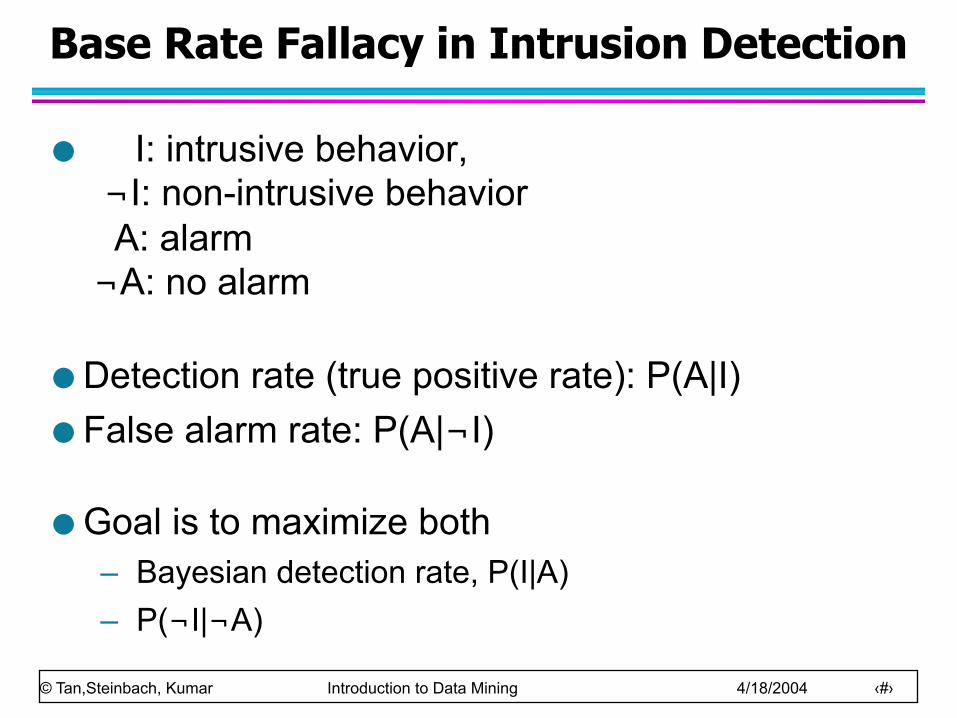
Base Rate Fallacy in Intrusion Detection
I: intrusive behavior, ¬I: non-intrusive behavior A: alarm ¬A: no alarm
Detection rate (true positive rate): P(A|I) False alarm rate: P(A|¬I)
Goal is to maximize both – Bayesian detection rate, P(I|A) – P(¬I|¬A)
© Tan,Steinbach, Kumar Introduction to Data Mining 4/18/2004 ‹#›
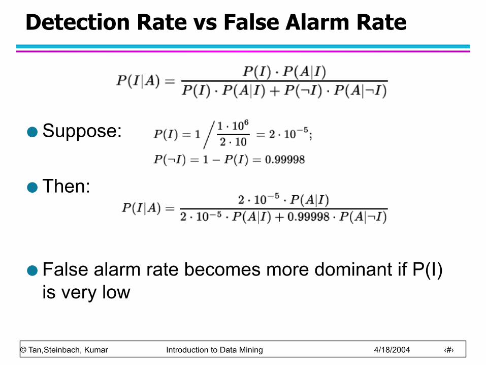
Detection Rate vs False Alarm Rate
Suppose:
Then:
False alarm rate becomes more dominant if P(I) is very low
© Tan,Steinbach, Kumar Introduction to Data Mining 4/18/2004 ‹#›
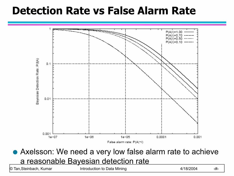
Detection Rate vs False Alarm Rate
Axelsson: We need a very low false alarm rate to achieve a reasonable Bayesian detection rate