lecture note on ``modern physics and machine learning
TRANSCRIPT

Lecture note on “Modern Physics and Machine Learning”
Please note that this lecture note is constantly updated.
last update: 2021/12/20
contact: Yuto Ashida (The University of Tokyo)


Contents
Chapter 1. Introduction 7
Chapter 2. Quantum mechanics review 102.1. Fundamental concepts 102.1.1. Quantum states 102.1.2. Observables 102.1.3. Time evolution 112.1.4. Measurement 112.1.5. Tensor product 122.2. Ensembles 122.2.1. Density operators 142.3. Distance measures 152.4. Example: Qubit 162.4.1. Bloch sphere 172.4.2. Unitary operator 172.4.3. Density operator 182.5. Example: Harmonic oscillator 182.5.1. Fock state 182.5.2. Coherent state 192.5.3. Squeezed state 20
Chapter 3. Theory of quantum measurement and open systems 233.1. Introduction: indirect measurement in qubit-boson model 233.2. Positive operator-valued measure 263.3. Completely positive trace-preserving (CPTP) map 263.4. Kraus operators and the equivalence to indirect measurement model 273.5. Bayesian inference and quantum measurement 283.5.1. Diagonal POVM and QND measurement 293.5.1.1. Convergence to measurement basis: wavefunction collapse 313.5.1.2. Born rule of collapsed states 323.5.2. Example: photon QND measurement in cavity QED 323.6. Continuous quantum measurement 343.6.1. Quantum trajectories 343.6.2. Quantum master equation 37
3

CONTENTS 4
3.6.3. Measurement dynamics vs Dissipation 383.6.4. Brief remark on non-Hermitian physics 393.6.5. Physical examples 39Example 1: Photon emission 40Example 2: Damped harmonic oscillator 40Example 3: Lossy many-body systems 413.6.6. Diffusive limit 423.6.6.1. Wiener process 423.6.6.2. Stochastic Schrödinger equation 423.6.6.3. Example: continuous position measurement 443.7. Master equation from Born-Markov approximations 453.8. Short remark on the validity of master equation approaches 483.9. Exercises 50Exercise 3.1 (Continuous position measurement: 2 points) 50Exercise 3.2 (Continuous measurement of indistinguishable particles: 2 points) 50Exercise 3.3 (Completely positivity: 1 point) 50
Chapter 4. Foundations of quantum optics 514.1. Introduction 514.2. Quantization of the electromagnetic field 514.2.1. Classical electromagnetism review 514.2.2. Quantization of electromagnetic fields 534.2.3. Commutation relations of quantized fields 554.3. Bosonic Gaussian states 564.3.1. Introduction: single mode 564.3.2. Multiple modes 58Characteristic function 58Bosonic Gaussian states 59Gaussian unitary operation 61Example: Gaussian pure state 624.3.3. Application to weakly interacting BEC 634.4. Fermionic Gaussian states 654.4.1. Introduction: single mode 654.4.2. Multiple modes 66Gaussian unitary operation 68Example: Fermionic Gaussian pure state 70Fermionic coherent states and characteristic function 714.4.3. Application to BCS superconductors 754.5. Variational principle 774.5.1. Introduction 774.5.2. Complex-valued variational manifold 78

CONTENTS 5
4.5.3. Real-valued variational manifold 794.5.4. Imaginary time evolution 804.5.5. Application to Gaussian states 824.6. Superconducting qubits 844.6.1. LC circuits 844.6.2. Josephson junction 854.6.3. Superconducting qubits: realizing effectively two-level systems 874.6.4. Light-matter interaction: circuit QED 884.7. Exercises 90Exercise 4.1 (Field commutation relations: 1 point) 90Exercise 4.2 (Single-mode bosonic pure Gaussian state: 1 point) 90Exercise 4.3 (McCoy’s formula: 1 point) 90Exercise 4.4 (Bosonic Gaussian states: 2 points) 90Exercise 4.5 (Generalized uncertainty relation: 1 point) 91Exercise 4.6 (Fermionic Gaussian states: 2 points) 91Exercise 4.7 (Conservation laws in variational analysis: 1 point) 91Exercise 4.8 (Variational time-evolution equations: 1 point) 91
Chapter 5. Quantum light-matter interaction 925.1. Classical electrodynamics review 925.1.1. Equations of motion 925.1.2. Redundancy in the dynamical variables and the Coulomb gauge 945.2. Quantized electrodynamics Hamiltonians 965.2.1. Quantum electrodynamics in the Coulomb gauge 965.2.2. Unitary transformation 975.2.3. Gauge transformation 985.3. Long wavelength approximation 995.3.1. Power-Zienau-Woolley transformation and dipole interaction 995.3.2. Matrix elements in different gauges and TRK sum rule 1005.3.3. Unitary transformations beyond gauge transformations 1025.3.3.1. Pauli-Fierz-Kramers transformation 1025.3.3.2. Asymptotically decoupling transformation 1035.3.4. Spontaneous emission: Wigner-Weisskopf theory 1045.4. Brief introduction to Cavity/Waveguide QED 1065.4.1. Two-level approximation: quantum Rabi model and Dicke model 1065.4.2. Rotating wave approximation: Jaynes-Cummings model 1085.4.3. Strong-coupling physics: asymptotic freedom 1085.4.4. Waveguide QED Hamiltonian and Spin-Boson model 1095.4.5. Circuit realizations 1105.5. Exercises 112Exercise 5.1 (PZW gauge without long-wave approximation: 2 points) 112

CONTENTS 6
Exercise 5.2 (Applications of TRK sum rule: 2 points) 113Exercise 5.3 (Mass renormalization in the asymptotically decoupled frame: 2 points) 113Exercise 5.4 (Spontaneous emission: 1 point) 114
Chapter 6. Machine learning and quantum science 1156.1. Introduction 1156.2. Basic concepts 1166.2.1. Supervised learning 1166.2.1.1. Function approximation, cost function, and training 116Example 1: Kernel method, support vector machine, and variational quantum circuits 117Example 2: Neural network and classifying phases of matter 1196.2.2. Unsupervised learning 120Example 3: Autoencoder 120Example 4: Restricted Boltzmann machine and neural network states 1216.3. Black-box optimization 122Random search 123Evolutionary strategy 123Genetic algorithm 124Differential evolution 1246.4. Exercises 127Exercise 6.1 (Gaussian kernel method: 1 point) 127Exercise 6.2 (Global optimization: 1 point) 127
Chapter 7. Reinforcement learning 1287.1. Introduction 1287.2. Motivating example 1287.3. Formalism: Markov decision process 1307.4. Value-based search 1317.4.1. Bellman equation 1317.4.2. Q learning 1327.4.3. Deep Q-learning 133Fixed target network 134Experience replay 1347.4.4. Physics application: quantum control of continuously monitored systems 1367.5. Policy-based search 1367.6. Black-box optimization in deep RL 1387.7. Some tips on implementation 1387.8. Exercise 139Exercise 7.1 (Mastering video game “Pong” via Black box optimization: 2 points) 139

CHAPTER 1
Introduction
In this course, we aim to learn some of the fundamental topics in modern quantum science, at theintersection of quantum optics, quantum information, and many-body physics. We will also try to coverelements of machine learning methods related to those topics, especially reinforcement learning that isgaining importance in the context of quantum control and other related fields. As I am theorist, the lec-tures will be given from a theoretical perspective, while I shall try to connect them with actual quantumexperiments in laboratory when appropriate. Below let me provide a brief overview and background ofthis course.
It is a wonderful time for studying quantum science; one can now routinely perform microscopicobservations and manipulations of genuine quantum systems in the laboratory. This has allowed us tostudy and understand quantum physics in a highly controlled and clean/coherent manner, paving the waytoward realizing future quantum devices, such as quantum computers or quantum simulators. At the sametime, such development necessarily requires us to understand physics of open systems as no physicalsystems can be completely isolated from their environments.
The system-environment interaction, or said differently, measurement backaction in general causeswavefunction collapse and is often detrimental to performing operations in quantum devices that are sup-posed to be coherent. Besides the role as the main obstacle for quantum technologies, however, suchcoupling to external degrees of freedom has often offered a new possibility of realizing some unique andexotic phenomena that are otherwise very difficult to realize in isolated systems. It is thus of fundamentalimportance to understand basics of open quantum systems, and it is this topic we aim to cover in Chapters2 and 3.
We will also cover foundations of quantum optics and quantum light-matter interactions in Chapters 4and 5. These topics will not only serve as a perfect example for a rather abstract theory of open quantumsystems presented in the previous Chapters, but also play central roles in the modern quantum technolo-gies. For example, superconducting qubits and circuit/cavity QED systems discussed there are currentlyone of the most promising building blocks toward realizing quantum computers. Moreover, theoreticalmethods we introduce there, including variational principles and bosonic/fermionic Gaussian states, arein fact useful theoretical tools to understand quantum many-body physics in condensed matter systems.
On another front, recent years have witnessed the emergence of a new powerful computational tech-nique, that is, machine learning. In particular, deep artificial neural networks are now routinely used toclassify images, translate languages, control robots, and even play video games at superhuman levels. Inthe context of physics, machine learning has found applications to predicting certain material properties,
7
1. INTRODUCTION 8
classifying phases of matter, and controlling quantum or classical physical systems. This is a rapidlygrowing area of research and it is of course impossible to cover all the topics in the emerging field of “ma-chine learning and physics” in the present course. Rather we here try to especially focus on one importantbranch of machine learning, namely, reinforcement learning.
Compared to a more elementary topic like supervised learning, reinforcement learning can be consid-ered as advanced concept since it requires neither teacher training a student nor a priori knowledge about aproblem at hand. In this sense, reinforcement learning can potentially find a novel solution to the problembeyond human abilities; said differently, machine can have kind of creativity. Indeed, when combinedwith deep neural networks, it has achieved superhuman performance in the game of Go. We will also seean illustrative example which indicates that the reinforcement learning holds great promise for controllingopen quantum systems. We will learn about some basic concepts of machine learning methods includingreinforcement learning in Chapters 6 and 7. Nevertheless, I would not pretend to teach specific techniquesfor numerical implementations, such as how to use existing libraries etc., but rather the main goal of thispart is to help you to gain intuition/key ideas behind the machine learning algorithms. I believe that theproper understanding of those algorithms is more important than learning about specific numerical tech-niques, as you should then be able to straightforwardly generalize/apply existing codes to problems atyour hand.

1. INTRODUCTION 9
Summary of Chapter 1This course attempts to cover the following topics:
• Review of (mostly) undergrad quantum mechanics (Chap. 2)• General theory of quantum measurement and Markovian open quantum systems (Chap. 3)• Brief introduction to non-Hermitian physics (Chap. 3)• Quantization of the electromagnetic field (Chap. 4)• General theory of bosonic and fermionic Gaussian states (Chap. 4)• Basics of time-dependent variational principles (Chap. 4)• Introduction to circuit/cavity/waveguide quantum electrodynamics (Chap. 4 and 5)• General theory of quantum light-matter interaction (Chap. 5)• Brief review of basic concepts in machine learning (Chap. 6)• Basics of (deep) reinforcement learning (Chap. 7)• Black-box optimization and its application to deep reinforcement learning (Chap. 6 and 7)• Deep reinforcement learning of a simple quantum control task (Chap. 7)
What is not included in this course:
• Non-Markovian or nonperturbative open quantum systems• Theory of non-Gaussian many-body states• Details about supervised/unsupervised learning• Model-based reinforcement learning algorithms• Details about policy-based reinforcement learning algorithms• Details about implementations for machine learning practitioners• and many other important topics...

CHAPTER 2
Quantum mechanics review
2.1. Fundamental concepts
2.1.1. Quantum states. Mathematically, a quantum state |ψ〉 is described as a vector in a HilbertspaceH:
Hilbert space. Hilbert space H is a vector space over the complex numbers C. It associates with aninner product 〈ψ|φ〉 of an ordered pair of vectors |ψ〉, |φ〉, which satisfies
• Conjugate symmetry: 〈φ|ψ〉 = 〈ψ|φ〉∗.• Linearity: 〈ψ|(a|φ〉+ b|ϕ〉) = a〈ψ|φ〉+ b〈ψ|ϕ〉.• Positivity: ‖|ψ〉‖ ≡
√〈ψ|ψ〉 > 0 for |ψ〉 6= 0.
It is also a complete metric space with respect to the distance defined by the norm d(|ψ1〉, |ψ2〉) =
‖|ψ1〉 − |ψ2〉‖.
Precisely speaking, we should consider a quantum state as a ray, which is an equivalent class of vec-tors that differ only by a nonzero complex constant factor. Since we are interested in a vector that has theunit norm, 〈ψ|ψ〉 = 1, this just means that its overall phase factor is physically irrelevant, i.e., it does notaffect an expectation value of a physical observable as we see below.
2.1.2. Observables. An observable is a physical quantity that can be measured and mathematicallydescribed as a self-adjoint operator. To see this, let us first introduce the notion of a Hermitian operator.
Hermiticity. A linear map O is a Hermitian operator if and only if 〈φ|O|ψ〉 = 〈ψ|O|φ〉∗ for ∀|ψ〉, |φ〉 ∈ H.
We can also express this condition as the self-adjoint condition O = O†, where we define the adjointO† of O by1
(2.1.1) 〈φ|Oψ〉 = 〈O†φ|ψ〉.
It is known that a self-adjoint operator has a spectral decomposition, i.e., its eigenstates form a completeorthonormal basis inH:
1Strictly speaking, for infinite-dimensional case, the self-adjointness not only requires the Hermiticity, but also the condition thatthe domains of O and O† are the same. Yet, this subtle difference does not cause problems at least in this course, so we shall usethe terms Hermitian or self-adjoint operators interchangeably.
10

2.1. FUNDAMENTAL CONCEPTS 11
(2.1.2) O =∑n
λnPn,
where λn is an eigenvalue and Pn is the projection operator onto the corresponding eigenspace satisfying
(2.1.3) PnPm = δnmPn
(2.1.4) Pn = P †n.
These projectors form a complete set such that they span the entire Hilbert space
(2.1.5)∑n
Pn = I ,
where I is the identity operator.
2.1.3. Time evolution. Time evolution of a quantum state is given by the Schrödinger equation (weset ~ = 1):
(2.1.6) id
dt|ψ(t)〉 = H|ψ(t)〉,
where H is a self-adjoint operator called the Hamiltonian. Its solution is easily obtained as
(2.1.7) |ψ(t)〉 = U(t)|ψ(0)〉,
(2.1.8) U(t) = e−iHt.
Here U(t) is the unitary operator, i.e., U(t)U †(t) = 1. As a result, the norm of a quantum state ispreserved:
(2.1.9) 〈ψ(0)|ψ(0)〉 = 〈ψ(t)|ψ(t)〉 = 1.
2.1.4. Measurement. A measurement of an observable O for a state |ψ〉 gives one of the eigenvaluesλn with probability
(2.1.10) pn = 〈ψ|Pn|ψ〉
and prepares the corresponding eigenstate:
(2.1.11)Pn|ψ〉√pn
.
Suppose that we perform the same measurement processes for the same state many times; then the expec-tation value 〈O〉 of the measurement outcomes is given by

2.2. ENSEMBLES 12
(2.1.12) 〈O〉 ≡∑n
λnpn =∑n
λn〈ψ|Pn|ψ〉 = 〈ψ|O|ψ〉,
where we used the spectral decomposition of O. Note that the phase factor of a vector |ψ〉 is irrelevant tothe expectation value as we mentioned above.
2.1.5. Tensor product. Consider two systems, A and B, whose Hilbert space is denoted byHA andHB , respectively. Then the composite system A + B is given by the tensor product HA ⊗HB , i.e., it isnow spanned by a quantum state |ψ〉A ⊗ |φ〉B with |ψ〉A ∈ HA and |φ〉B ∈ HB .
To understand the notion of tensor product, it is useful to consider a simple example of a pair of two-level systems. Let us describe a quantum state |ψ〉 of a two-level system spanned by |0〉, |1〉 as a vectorrepresentation
(2.1.13) |ψ〉 = a|0〉+ b|1〉 ⇐⇒ |ψ〉 =
(a
b
).
Then suppose that we have the following states in each of the two-level systems
(2.1.14) |ψ〉A =
(u
v
), |φ〉B =
(x
y
).
The resulting composite state is a four-dimensional vector given by
(2.1.15) |ψ〉A ⊗ |φ〉B =
ux
uy
vx
vy
.
Similarly, if we have the operators
(2.1.16) A =
(a b
c d
), B =
(e f
g h
),
the composite operator is a 4× 4 matrix given by
(2.1.17) A⊗ B =
ae af be bf
ag ah bg bh
ce cf de df
cg ch dg dh
.
2.2. Ensembles
The formulation of quantum mechanics in the previous section is provided for an ideal situation,in which all the microscopic quantum degrees of freedom in a system of interest are accessible to an

2.2. ENSEMBLES 13
observer; in other words, this formulation is supposed to deal with a completely isolated (or closed)quantum system. However, in real world, what we can observe is only a small part of an entire quantumsystem and this small quantum system interacts with external degrees of freedom that one cannot handle,i.e., a real quantum system necessarily behaves as an open system.
To motivate this, consider the following quantum state in the composite space of a pair of two-levelsystems:
(2.2.1) |ψ〉AB =1√2
(|0〉A|0〉B + |1〉A|1〉B) .
Suppose that we have access to a two-level system A, but not for B and thus we know nothing about astate of B. In this case, only an observable acting on A is of interest and we expect that there exists a self-consistent theoretical description within A. To see this, consider the expectation value of an observableOA that (nontrivially) acts only on A:
〈OA〉 ≡AB 〈ψ|OA ⊗ IB|ψ〉AB(2.2.2)
=1
2
(A〈0|OA|0〉A + A〈1|OA|1〉A
).(2.2.3)
We now see that the expectation value can be obtained by solely dealing with a quantum state in A.However, this value is different from the usual expression for the expectation value with respect to a purestate, but can be represented as the trace over the following density operator ρA:
(2.2.4) 〈OA〉 = TrA[ρAOA] ≡∑i=0,1
A〈i|ρAOA|i〉A
with
(2.2.5) ρA ≡ TrB[|ψ〉ABAB〈ψ|] =1
2(|0〉AA〈0|+ |1〉AA〈1|) .
We should interpret ρA as an ensemble of possible quantum states occurring with the equal probability.This means that the expectation value is equal to the ensemble average (or incoherent mixture) over thecorresponding expectation values with respect to two states:
(2.2.6) 〈OA〉 =1
2
∑i=0,1
A〈i|OA|i〉A.
In other words, an initially pure quantum state should in general be described as an incoherent mixture ofdifferent pure states after it interacts with unknown external degrees of freedom. For instance, the relativephase in the original pure state |ψ〉AB is no longer accessible and there will be no interference effects inρA. The partial trace over B above corresponds to such procedure of discarding knowledge about externaldegrees of freedom; since an observer cannot access to environment degrees of freedom, the best one can

2.2. ENSEMBLES 14
do is to take the unbiased summation over quantum states in B. As we see later, this process lies at theheart of important phenomenon called decoherence.
2.2.1. Density operators. In general, an operator ρ acting on a Hilbert space H is called a densityoperator if it satisfies the following properties:
• ρ = ρ†
• ρ ≥ 0 ⇐⇒ 〈ψ|ρ|ψ〉 ≥ 0 ∀|ψ〉 ∈ H• Tr(ρ) = 1
If a quantum state is a pure state |ψ〉, the corresponding density operator is given by
(2.2.7) ρ = |ψ〉〈ψ|
and satisfies the following condition
(2.2.8) ρ2 = ρ.
It is often useful to note the fact that there is an orthonormal basis that diagonalizes ρwith nonnegativeand real eigenvalues whose summation gives one:
(2.2.9) ρ =∑i
pi|i〉〈i|, 〈i|j〉 = δij ,∑i
pi = 1.
The coefficients pi can naturally be interpreted as the probability weight associated with ρ, which is theincoherent mixture of pure states |i〉.
It is also worthwhile to note that a density operator satisfies the convexity; using two density matricesρ1,2, one can construct another density matrix by a linear combination:
(2.2.10) ρ(λ) = λρ1 + (1− λ)ρ2, 0 ≤ λ ≤ 1.
Indeed, it obviously satisfies the self-adjoint condition ρ(λ) = ρ†(λ) and the normalization Tr[ρ(λ)] = 1.The positivity is also satisfied because
(2.2.11) 〈ψ|ρ(λ)|ψ〉 = λ〈ψ|ρ1|ψ〉+ (1− λ)〈ψ|ρ2|ψ〉 ≥ 0, ∀|ψ〉 ∈ H
We note that for any density operator ρA one can perform its purification, that is, one can construct acomposite pure state |Ψ〉AB that gives ρA upon doing a partial trace over degrees of freedom in B. Usingthe expression (2.2.9), one possible purification is given by
(2.2.12) |Ψ〉AB =∑i
√pi|i〉A ⊗ |φi〉B
with orthonormal states in B

2.3. DISTANCE MEASURES 15
(2.2.13) B〈φi|φj〉B = δij .
Indeed, it leads to the required relation
(2.2.14) ρA = TrB[|Ψ〉ABAB〈Ψ|].
2.3. Distance measures
Suppose that we have two density operators ρ and σ. Since a density operator satisfies the positivity,there exists the square-root operator
√ρ following from the condition (
√ρ)2 = ρ. For instance, in the
diagonal basis, it is given by
(2.3.1)√ρ =
∑i
√pi|i〉〈i|.
Building on this, one can quantify the distinguishability of two ensembles via the following measureknown as the fidelity:
(2.3.2) F (ρ, σ) ≡(
Tr
[√√ρσ√ρ
])2
.
Alternatively, one can represent the fidelity as the L1 norm as follows:
(2.3.3) F (ρ, σ) =∣∣∣√σ√ρ∣∣∣2
1
where we define the L1 norm by
(2.3.4)∣∣∣A∣∣∣
1≡ Tr
[√A†A
].
A useful expression of the L1 norm is
(2.3.5)∣∣∣A∣∣∣
1= maxU
∣∣∣Tr[U †A
]∣∣∣ ,where U is unitary. One can check this expression by using the singular value decomposition of A.
It satisfies the following properties
• F (ρ, σ) = F (σ, ρ)
• 0 ≤ F (ρ, σ) ≤ 1, F (ρ, ρ) = 1
• F (ρ, σ) =(∑
i
√piqi)2 if [ρ, σ] = 0
where pi and qi are eigenvalues of ρ and σ, respectively, and we define the commutator by
(2.3.6) [A, B] ≡ AB − BA.

2.4. EXAMPLE: QUBIT 16
Note that the last relation for commuting density operators is nothing but the usual fidelity between (clas-sical) probability distributions. The upper bound in the second relation F ≤ 1 follows from the relation
(2.3.7) F (ρ, σ) ≤ Tr(ρ)Tr(σ) = 1,
which can be shown by using the relation (2.3.5) and the Cauchy-Schwarz inequality:
(2.3.8) F (ρ, σ) =
∣∣∣∣Tr
[(√ρU)†√
σ
]∣∣∣∣2 ≤ Tr
((√ρU)† (√
ρU))
Tr(√
σ√σ)
= Tr(ρ)Tr(σ).
If one of the density operators is pure ρ = |ψ〉〈ψ|, then the fidelity reduces to
(2.3.9) F (ρ, σ) = 〈ψ|σ|ψ〉.
In particular, when the other one is also pure σ = |φ〉〈φ|, it simplifies to the overlap
(2.3.10) F (ρ, σ) = |〈ψ|φ〉|2.
Finally, there exists a useful general relation between the fidelity and the trace norm:
(2.3.11) F (ρ, σ) ≤ 1− 1
4|ρ− σ|21 .
It will be a good exercise for you to check this inequality (hint: you may use the triangle inequality for thetrace norm, the Cauchy-Schwarz inequality, and the relation (2.3.5)).
2.4. Example: Qubit
Let us illustrate the fundamental notions introduced above by discussing the minimal example: atwo-dimensional Hilbert space spanned by orthonormal quantum states |0〉, |1〉. Since an overall phasefactor is irrelevant, a generic normalized state in this space is described as
(2.4.1) |ψ(θ, φ)〉 = cos
(θ
2
)|0〉+ eiφ sin
(θ
2
)|1〉 =
(cos(θ2
)eiφ sin
(θ2
) ) .The angles θ and φ characterize the probability weights for each state and the relative phase between twostates, respectively.
This represents a quantum counterpart of classical bit, namely, qubit. For instance, the spin-1/2 degreeof freedom of electron or two internal states in photon polarizations exactly behave as the qubit. However,as we will see in later Chapters, qubits in many of state-of-the-art quantum computers, such as supercon-ducting qubits, actually use two lowest levels in a larger Hilbert space. Thus, it is important to keep inmind that they do not perfectly operate as two-level systems in strict sense, but rather effectively play therole of qubits with a certain (usually high) fidelity.
2.4. EXAMPLE: QUBIT 17
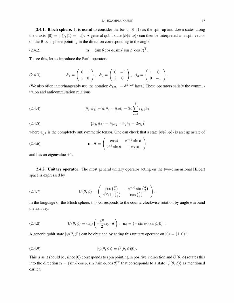
2.4.1. Bloch sphere. It is useful to consider the basis |0〉, |1〉 as the spin-up and down states alongthe z axis, |0〉 = | ↑〉, |1〉 = | ↓〉. A general qubit state |ψ(θ, φ)〉 can then be interpreted as a spin vectoron the Bloch sphere pointing in the direction corresponding to the angle
(2.4.2) n = (sin θ cosφ, sin θ sinφ, cos θ)T.
To see this, let us introduce the Pauli operators
(2.4.3) σ1 =
(0 1
1 0
), σ2 =
(0 −ii 0
), σ3 =
(1 0
0 −1
).
(We also often interchangeably use the notation σ1,2,3 = σx,y,z later.) These operators satisfy the commu-tation and anticommutation relations
(2.4.4) [σi, σj ] = σiσj − σj σi = 2i3∑
k=1
εijkσk
(2.4.5) σi, σj = σiσj + σj σi = 2δij I
where εijk is the completely antisymmetric tensor. One can check that a state |ψ(θ, φ)〉 is an eigenstate of
(2.4.6) n · σ =
(cos θ e−iφ sin θ
eiφ sin θ − cos θ
)and has an eigenvalue +1.
2.4.2. Unitary operator. The most general unitary operator acting on the two-dimensional Hilbertspace is expressed by
(2.4.7) U(θ, φ) =
(cos(θ2
)−e−iφ sin
(θ2
)eiφ sin
(θ2
)cos(θ2
) ).
In the language of the Bloch sphere, this corresponds to the counterclockwise rotation by angle θ aroundthe axis n0:
(2.4.8) U(θ, φ) = exp
(− iθ
2n0 · σ
), n0 = (− sinφ, cosφ, 0)T.
A generic qubit state |ψ(θ, φ)〉 can be obtained by acting this unitary operator on |0〉 = (1, 0)T:
(2.4.9) |ψ(θ, φ)〉 = U(θ, φ)|0〉.
This is as it should be, since |0〉 corresponds to spin pointing in positive z direction and U(θ, φ) rotates thisinto the direction n = (sin θ cosφ, sin θ sinφ, cos θ)T that corresponds to a state |ψ(θ, φ)〉 as mentionedearlier.
2.5. EXAMPLE: HARMONIC OSCILLATOR 18
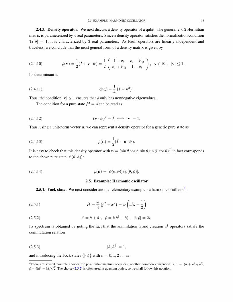
2.4.3. Density operator. We next discuss a density operator of a qubit. The general 2× 2 Hermitianmatrix is parameterized by 4 real parameters. Since a density operator satisfies the normalization conditionTr[ρ] = 1, it is characterized by 3 real parameters. As Pauli operators are linearly independent andtraceless, we conclude that the most general form of a density matrix is given by
(2.4.10) ρ(v) =1
2(I + v · σ) =
1
2
(1 + v3 v1 − iv2
v1 + iv2 1− v3
), v ∈ R3, |v| ≤ 1.
Its determinant is
(2.4.11) detρ =1
4
(1− v2
).
Thus, the condition |v| ≤ 1 ensures that ρ only has nonnegative eigenvalues.The condition for a pure state ρ2 = ρ can be read as
(2.4.12) (v · σ)2 = I ⇐⇒ |v| = 1.
Thus, using a unit-norm vector n, we can represent a density operator for a generic pure state as
(2.4.13) ρ(n) =1
2(I + n · σ).
It is easy to check that this density operator with n = (sin θ cosφ, sin θ sinφ, cos θ)T in fact correspondsto the above pure state |ψ(θ, φ)〉:
(2.4.14) ρ(n) = |ψ(θ, φ)〉〈ψ(θ, φ)|.
2.5. Example: Harmonic oscillator
2.5.1. Fock state. We next consider another elementary example - a harmonic oscillator2:
(2.5.1) H =ω
4
(p2 + x2
)= ω
(a†a+
1
2
)(2.5.2) x = a+ a†, p = i(a† − a), [x, p] = 2i.
Its spectrum is obtained by noting the fact that the annihilation a and creation a† operators satisfy thecommutation relation
(2.5.3) [a, a†] = 1,
and introducing the Fock states |n〉 with n = 0, 1, 2 . . . as
2There are several possible choices for position/momentum operators; another common convention is x = (a + a†)/√
2,p = i(a† − a)/
√2. The choice (2.5.2) is often used in quantum optics, so we shall follow this notation.

2.5. EXAMPLE: HARMONIC OSCILLATOR 19
(2.5.4) a|n〉 =√n|n− 1〉, a†|n〉 =
√n+ 1|n+ 1〉,
(2.5.5) a†a|n〉 = n|n〉.
In particular, for the ground state with n = 0, also called as vacuum state, we get
(2.5.6) a|0〉 = 0.
The corresponding eigenvalue is
(2.5.7) En = ω
(n+
1
2
).
2.5.2. Coherent state. Fock states are eigenstates of the number operator n ≡ a†a, while one canalso construct an eigenstate of the annihilation operator a, the coherent state:
(2.5.8) |α〉 ≡∞∑n=0
αn√n!e−|α|
2/2|n〉, α ∈ C
(2.5.9) a|α〉 = α|α〉.
The occupation probabilities in the Fock basis obey the Poisson distribution with mean n ≡ |α|2:
(2.5.10) P (n) =nn
n!e−n.
Note that |α〉 is not an eigenstate of the creation operator a†, which acts as
(2.5.11) a†|α〉 =
(∂
∂α+ α∗
)|α〉.
The vacuum state |0〉 is a special example of a coherent state with α = 0. In fact, a general coherentstate can be obtained by acting the following displacement operator on the vacuum:
(2.5.12) D(α) = eαa†−α∗a = e−|α|
2/2eαa†e−α
∗a = e|α|2/2e−α
∗aeαa†,
(2.5.13) D(α)|0〉 = |α〉.
The displacement operator satisfies the following properties
• D†(α) = D−1(α) = D(−α)
• D†(α)aD(α) = a+ α
• D†(α)a†D(α) = a† + α∗
• D(α+ β) = e−(αβ∗−α∗β)/2D(α)D(β) = e(αβ∗−α∗β)/2D(β)D(α)

2.5. EXAMPLE: HARMONIC OSCILLATOR 20
The last relation follows from the Baker-Campbell-Hausdorff (BCH) formula:
(2.5.14) eA+B = eAeBe−12
[A,B] = eBeAe12
[A,B].
In particular, note that two different coherent states are not orthogonal:
(2.5.15) |〈β|α〉| = e−|α−β|2/2.
2.5.3. Squeezed state. To motivate the notion of a squeezed state, consider the following Hamilton-ian that includes the so-called A2 term on top of the usual harmonic oscillator3:
(2.5.16) H = ωa†a+g2
2ωA2, A ≡ a† + a.
Since this Hamiltonian is still quadratic in terms of creation or annihilation operators, one can diagonalizeit by using the unitary transformation often called as the Bogoliubov transformation:
(2.5.17) b = cosh ra+ sinh ra† ≡ U †r aUr,
(2.5.18) er =
√Ω
ω, Ω =
√ω2 + 2g2, Ur = e
r2(a†2−a2).
Note that the new annihilation/creation operators b, b† satisfy the canonical commutation relation
(2.5.19) [b, b†] = 1.
Thus, the above Hamiltonian is diagonalized as
(2.5.20) H = Ωb†b+ const.,
where we use a = cosh rb − sinh rb†. The unitary operator U is an example of the squeezing operator,and the transformed ground state is given by the squeezed vacuum
(2.5.21) |0〉b ≡ U †r |0〉 = er2(a2−a†2)|0〉 = e
ir4
(xp+px)|0〉.
To see the reason why it represents “squeezing”, it is useful to rewrite the Hamiltonian in terms ofposition and momentum operators as (aside constant)
(2.5.22) H =ω
4
(p2 + x2
)+g2
2ωx2 =
ω
4
(p2 +
Ω2
ω2x2
).
3We will later see that this Hamiltonian is relevant to the minimal setup of cavity quantum electrodynamics in the Coulombgauge.

2.5. EXAMPLE: HARMONIC OSCILLATOR 21
This means that the above Hamiltonian is nothing but the usual harmonic oscillator, but with a tighterpotential with Ω2/ω2 ≥ 1. Consequently, the ground state |0〉b is more strongly confined in the x directioncompared with the original vacuum |0〉. Due to the uncertainty relation, this results in an inevitable“expansion” in the p direction. More explicitly, we get
(2.5.23) Ur
(x
p
)U †r =
(e−rx
erp
).
Because position and momentum operators are interchangeable in harmonic oscillators, one can simi-arly consider a squeezing in a general direction on the x-p plane. A general squeezing operator is givenby
(2.5.24) S(ζ) ≡ e(ζa†2−ζ∗a2)/2, ζ = reiθ ∈ C,
which transforms the annihilation and creation operators by
(2.5.25) S†(ζ)aS(ζ) = cosh ra+ eiθ sinh ra†.

2.5. EXAMPLE: HARMONIC OSCILLATOR 22
Summary of Chapter 2Section 2.1 Fundamental concepts
• A quantum state is described as a vector (or precisely speaking, ray) in a Hilbert space.• An observable is described by a self-adjoint operator on a Hilbert space.• Time evolution of a quantum state is given by the Schrödinger equation governed by the self-
adjoin operator called the Hamiltonian.• A measurement process is described as an orthogonal projection onto the corresponding
eigenspace.• A composite system is described by the tensor product.
Section 2.2 Ensembles
• When only a small part of an entire quantum system is accessible, a quantum state is describedby an ensemble called density operator.• A density operator is self-adjoint, positive, and satisfies the convexity.• Any density operator can be purified, i.e., one can construct a composite pure state that gives
a density operator of interest upon doing a partial trace.
Section 2.3 Distance measures
• The distinguishability of two quantum states can be quantified by the fidelity.• The fidelity can be related to other distance measures such as the L1 norm through the
(in)equalities.
Section 2.4 Qubit
• A general qubit pure state can be represented as a unit-norm vector on the Bloch sphere.• Similarly, a density operator of a qubit can be represented as unnormalized vector v in 3D
space with |v| ≤ 1.
Section 2.5
• Eigenspectrum of a harmonic oscillator is given by using the annihilation and creation opera-tors.• An energy eigenstate is given by a Fock state.• An eigenstate of the annihilation operator is a coherent state.• When a quadratic term is added to the Hamiltonian, eigenstate is in general squeezed along a
certain direction on the position-momentum space.

CHAPTER 3
Theory of quantum measurement and open systems
3.1. Introduction: indirect measurement in qubit-boson model
In this Chapter, we give an introduction to theory of quantum measurement and open systems. Beforeproceeding to a general formalism, let us first consider a simple motivating example, where a systemof interest is a single qubit and it interacts with a “meter” degree of freedom modeled by a harmonicoscillator. Physically, this may be considered as a toy model for spontaneous emission process, in whichthe two-level system (qubit) can be considered as an atom that can emit a photon into a simplified single-mode electromagnetic mode playing the role of the meter.
The model Hamiltonian is
(3.1.1) HJC =~∆
2σz + ~ωcb†b+ ~γ(σ−b† + σ+b),
(3.1.2) σ± =σx ± iσy
2, [b, b†] = 1,
which is known as the Jaynes-Cummings model. In fact, this model can be microscopically derived fromthe fundamental light-matter Hamiltonian after performing certain approximations, as we will see in laterChapters. A notable feature of this Hamiltonian is that it conserves the excitation number
(3.1.3) Nex =1
2(σz + 1) + b†b.
To be concrete, suppose that the initial state is the product state of the excited qubit and the photonvacuum
(3.1.4) ρtot(0) = |e〉〈e| ⊗ |0〉〈0|,
which belongs to the excitation manifold with Nex = 1. The evolved state is
(3.1.5) ρtot(t) = U ρtot(0)U †, U = e−iHJCt.
We then perform a projection measurement on the meter degree of freedom; since we consider thesector with Nex = 1, there are only two possible outcomes corresponding to the following projectionoperators
(3.1.6) P0 = |0〉〈0|, P1 = |1〉〈1|.
23

3.1. INTRODUCTION: INDIRECT MEASUREMENT IN QUBIT-BOSON MODEL 24
They satisfy the completeness relation (within the Hilbert space of interest here):
(3.1.7) IA =1∑
m=0
Pm.
The postmeasurement (unnormalized) state with outcome m ∈ 0, 1 is given by
(3.1.8) Em(ρS(0)) ≡ TrA
[(IS ⊗ Pm
)ρtot(t)
(IS ⊗ Pm
)],
where we note that the trace TrA is taken only over the meter degree of freedom, and Em is defined by thelinear map acting on the system initial state:
(3.1.9) ρS(0) = |e〉〈e|.
Physically, the linear map Em represents the nonunitary evolution of the system conditioned on measure-ment outcome m. The outcome occurs with the probability
(3.1.10) pm = TrS [Em(ρS(0))] .
The normalized postmeasurement state is
(3.1.11) ρS,m =Em(ρS(0))
pm.
We can rewrite this nonunitary evolution in a more convenient way. To this end, we introduce theKraus operators Mm by
(3.1.12) Mm = 〈m|U |0〉,
where note that the inner product is taken only over the meter degree of freedom and thus Mm is anoperator that acts on the system Hilbert space. This leads to the expression of the postmeasurement state
Em(ρS(0)) = TrA
[(IS ⊗ Pm
)U ρS(0)⊗ |0〉〈0|U †
(IS ⊗ Pm
)](3.1.13)
= 〈m|U |0〉ρS(0)〈0|U †|m〉(3.1.14)
= MmρS(0)M †m.(3.1.15)
The probability is then expressed by the positive operator-valued measure (POVM) Em as follows
(3.1.16) pm = TrS
[ρS(0)Em
], Em = M †mMm.
Importantly, Em are in general nonorthogonal and thus can be considered as a generalization of projectionmeasurement operators Pm. The Kraus operators and the POVMs satisfy the completeness condition:
(3.1.17)1∑
m=0
Em =
1∑m=0
M †mMm = IS ,

3.1. INTRODUCTION: INDIRECT MEASUREMENT IN QUBIT-BOSON MODEL 25
leading to
(3.1.18)1∑
m=0
pm = 1.
So far, we discuss the time evolution that is conditioned on a certain measurement outcome. Anotherimportant concept is the nonunitary evolution that is unconditioned on measurement outcomes, oftencalled the nonselective evolution defined by
(3.1.19) E(ρS(0)) ≡1∑
m=0
Em(ρS(0)) =1∑
m=0
MmρS(0)M †m.
This mapping E satisfies the linearity, positivity1, and trace-preserving properties Tr[E(ρ)] = 1; we willgeneralize its notion as the completely positive trace preserving (CPTP) map later.
As shown below, it is often useful to consider the so-called continuous measurement limit, for whichwe take γ → ∞ and τ → 0 while keeping γ2τ finite. Here, we denote τ as the (short) time durationfor a single whole process of the indirect measurement. In this limit, at the leading order of γτ 1, thepostmeasurement state when a photon is detected is given by
(3.1.20) ρS,1 =τLρS(τ)L†
p1,
where
(3.1.21) ρS(τ) = US |e〉〈e|U †S , US = e−i∆σzτ/2,
and we define the so-called jump operator by
(3.1.22) L ≡√γ2τ σ−.
In this limit, the Kraus operator corresponding to photon detection (m = 1) is given by
(3.1.23) M1 '√τL
while the probability is
(3.1.24) p1 = τTrS
[LρS(τ)L†
].
This nonunitary evolution (often called quantum jump) corresponds to the process that, due to the photondetection, an observer acquires the information that the system (two-level atom) de-excites and is thusprojected onto the ground state, i.e., ρS,1 = |g〉〈g|.
Meanwhile, when a photon is not detected during the time interval τ , the postmeasurement state isgiven by
(3.1.25) ρS,0 =1
p0
[US |e〉〈e|U †S −
τ
2
L†L, ρS(τ)
],
1A linear operator O ∈ L(H) acting on the Hilbert space H is positive, O ≥ 0, iff 〈ψ|O|ψ〉 ≥ 0 for ∀|ψ〉 ∈ H. A linearmapping E : L(H)→ L(H) is then said to be positive, E ≥ 0, iff E(O) ≥ 0 for any positive operator O ≥ 0.

3.3. COMPLETELY POSITIVE TRACE-PRESERVING (CPTP) MAP 26
and the probability is
(3.1.26) p0 = 1− τTrS
[LρS(τ)L†
].
The corresponding Kraus operator is
(3.1.27) M0 = 1− iHeffτ/~
where we introduce the non-Hermitian effective Hamiltonian by
(3.1.28) Heff =~∆
2σz − i
2L†L =
~∆
2σz − iγ
2|e〉〈e|.
It is important to note that, even in this no-photon-counting process, an observer actually gains the infor-mation about the system in the sense that she/he knows that no spontaneous emission has occurred duringthe time interval τ . This information acquisition indicates that the system is more likely to be in the groundstate than in the excited state. It is this tendency that is ascribed to the measurement backaction, which iscaptured by the non-Hermitian term in Heff .
3.2. Positive operator-valued measure
From now on we present a general theory of quantum measurement by considering each notion intro-duced in the previous section in a more abstract manner. To begin with, motivated by the above simpleexample, we characterize the POVMs Em by the following properties
• Em = E†m
• Em ≥ 0
•∑
m Em = I
Recall that they are not orthogonal in general. Using the POVMs, the probability of observing measure-ment outcome m is given by
(3.2.1) pm = Tr[Emρ].
We note that the Hermiticity and positivity of POVMs ensures that pm are real and nonnegative, while thecompleteness relation ensures the normalization
∑m pm = 1; altogether, pm can indeed be interpreted as
probabilities.
3.3. Completely positive trace-preserving (CPTP) map
We next introduce the notion of a completely positive trace-preserving (CPTP) map E in a generalway. We shall first give a formal definition of the CPTP map E . Consider a Hilbert space H and a set oflinear operators L(H) acting onH. Since a linear map E : L(H)→ L(H) is supposed to represent certaintime evolution, it should map a density operator ρ ∈ L(H) to another density operator in the same Hilbertspace. This means that E must be (at least) positive E ≥ 0. Since the system of interest is in practicejust part of the whole world (i.e., ultimately there always exist external degrees of freedom other than thesystem), we must also ensure that E is positive even when it acts on part of a larger Hilbert space. Thus,

3.4. KRAUS OPERATORS AND THE EQUIVALENCE TO INDIRECT MEASUREMENT MODEL 27
it is in fact legitimate to require a stronger condition known as the completely positivity2. Altogether, wedefine the CPTP map by the following conditions:
• E(aρ+ bσ) = aE(ρ) + bE(σ)
• E(ρ) is a density operator, i.e., it is self-adjoint, positive, and satisfies Tr[E(ρ)] = Tr[ρ] = 1.• E is completely positive, i.e., a linear map E ⊗ I : L(H ⊗HA) → L(H ⊗HA) is positive for
arbitrary (additional) Hilbert spaceHA. Here, I is the identity operator acting on L(HA).
It is worthwhile to note that, if the completely positivity is not satisfied, an initially entangled state inH⊗HA can lead to negative probabilities after the mapping E ⊗I (see e.g., Peres, PRL 77, 1413 (1996)).In this sense, the completely positivity is necessary to ensure that E indeed gives physically reasonabletime evolution even when the initial state is correlated with external world.
We recall that the simple example discussed before indicates that E has an operator-sum representa-tion (3.1.19) with the Kraus operators Mm. The map E then physically represents the nonselective (orunconditional) nonunitary evolution that is ensemble averaged over all the possible measurement out-comes m. These expressions follow from the originally unitary evolution in the larger Hilbert space. Thisobservation naturally motivates the question: given a general CPTP map E acting on a Hilbert space H,is it possible to embed H into a larger Hilbert space and to construct a unitary evolution on this extendedsystem that reduces to E upon tracing out the degrees of freedom outsideH? One can answer this questionin the affirmative way, as we briefly explain in the next section.
3.4. Kraus operators and the equivalence to indirect measurement model
There is an equivalence between a CPTP map and an indirect measurement model in an extendedHilbert space (exemplified by the simple model above). This means that any nonunitary dynamics ofopen quantum systems can be considered as a part of a larger closed system equipped with orthogonalprojection measurements.
To state this in a more formal manner, let Emm∈M be a set of linear mappings acting on a vectorspace spanned by a linear operator L(H). Suppose that they satisfy the following conditions:
• E ≡∑
m Em is trace preserving, i.e., Tr[E(O)] = Tr[O] for ∀O ∈ L(H).• Em is completely positive for ∀m ∈M .
Then, one can show that [Hellwig & Kraus, Comm. Math. Phys. 16, 142 (1970); Kraus, Ann. Phys. 64,311 (1971); Stinespring, Proc. Amer. Math. Soc. 6, 211 (1955)], if and only if Emm∈M satisfies the
above conditions, there is the following indirect measurement model with some set ofHA, ρA, U ,
Pm
m∈M
(often called Stinespring representation):
(3.4.1) Em(ρ) = TrHA
[(I ⊗ Pm
)U (ρ⊗ ρA) U †
(I ⊗ Pm
)],
where HA is a Hilbert space and ρA is a density operator for HA, U is a unitary operator acting onH ⊗ HA, and
Pm
m∈M
is a set of projection operators on the subspace of HA corresponding to eachmeasurement outcome m.
2We remark that positive maps are not necessarily completely positive; we leave constructing such a map to Exercise of thisChapter.

3.5. BAYESIAN INFERENCE AND QUANTUM MEASUREMENT 28
For a given CPTP map E =∑
m Em, this statement guarantees the existence of a meterA and a unitaryoperator, which will reproduce E upon tracing out the meter degrees of freedom. However, the constructedmeter and the unitary operator are still rather mathematical objects; to deal with a real physical system, ingeneral we need to perform careful analysis of the interaction between the measured system and the meterin light of each physical situation. We will demonstrate such an analysis for a simple example later.
As shown above, the most general measurement process is described by a set of the completely posi-tive maps Em whose nonselective mapping E =
∑m Em is trace reserving. Then, it is useful to note that
the measurement process always permits the following representation (often called Kraus representation):
(3.4.2) Em(ρ) =∑k
Mm,kρM†m,k.
To see this, it suffices to employ the spectral decomposition
(3.4.3) ρA =∑i
ci|ψi〉AA〈ψi|, Pm =∑j
|φm,j〉AA〈φm,j |,
where |ψi〉A and |φm,j〉A are orthonormal basis inHA. Then, introducing the Kraus operators by
(3.4.4) Mm,k ≡ Mm,(i,j) =√ciA〈φm,j |U |ψi〉A,
one can show that the (unnormalized) postmeasurement state in Eq. (3.4.1) can be written as in Eq. (3.4.2).The Kraus representation allows us to express the POVMs by the operator-sum form as
(3.4.5) Em =∑k
M †m,kMm,k,∑m
Em = I .
The normalized postmeasurement state is given by
(3.4.6) ρm =Em(ρ)
pm
with the probability of observing measurement outcome m being
(3.4.7) pm = Tr[ρEm].
Conversely, one can show that any Kraus representation can be transformed to some Stinespring represen-tation.
3.5. Bayesian inference and quantum measurement
Bayesian inference is usually discussed in the context of classical estimation theory. In this section,we see that a certain class of quantum measurement processes is in fact completely equivalent to Bayesianinference. A prominent example includes the quantum nondemolition (QND) measurement that has beenrealized in a beautiful cavity QED experiment (2012 Nobel Prize), as we briefly discuss below.

3.5. BAYESIAN INFERENCE AND QUANTUM MEASUREMENT 29
3.5.1. Diagonal POVM and QND measurement. To motivate the notion of QND measurement,consider a measurement process whose POVM and Kraus operators can be diagonally decomposed into
(3.5.1) Em =∑j
cm,j |ψj〉〈ψj |, Mm,k =∑j
c′m,k,j |ψj〉〈ψj |
by using the common orthogonal basis |ψj〉 with some coefficients cm,j =∑
k |c′m,k,j |2. Let us denotethe probabilities associated with the projection operators by
(3.5.2) P (j) = Tr[Pj ρ], Pj = |ψj〉〈ψj |
and write the conditional probability distribution of measurement outcomes for |ψj〉 as
(3.5.3) P (m|j) = Tr[Emρj ], ρj =Pj ρPjP (j)
.
Similarly, let P (j|m) be the conditional probability distribution of finding a quantum state in |ψj〉 afterobtaining measurement outcome m:
(3.5.4) P (j|m) = Tr[Pj ρm], ρm =Em(ρ)
P (m).
Then, it satisfies Bayes’ theorem
(3.5.5) P (j|m) =P (m|j)P (j)
P (m), P (m) =
∑i
P (m|i)P (i).
This follows from the relation
(3.5.6) P (j|m) =Tr[PjEm(ρ)]
P (m)=
Tr[Em(P (j)ρj)]
P (m)=
Tr[Emρj ]
P (m)P (j) =
P (m|j)P (j)
P (m).
If we perform measurement process n times whose measurement outcomes are m = m1,m2, . . . ,mn,we obtain
(3.5.7) Pn(j|m) =
∏nl=1 P (ml|j)P0(j)
P (m), P (m) =
∑i
n∏l=1
P (ml|i)P0(i).
This is nothing but the usual chain rule of Bayes’ relation. Hence, we can reconstruct the probabilitydistribution Pn(j|m) of the postmeasurement quantum state in the |ψj〉 basis along with the same lineof classical estimation theory.
A quantum nondemolition (QND) measurement is an important class of quantum measurements thatsatisfies the above diagonal condition (3.5.1) and thus essentially reduces to the problem of Bayesian infer-ence. To introduce the notion of QND measurement, consider a measurement process whose nonselectiveevolution is

3.5. BAYESIAN INFERENCE AND QUANTUM MEASUREMENT 30
(3.5.8) E(ρ) = TrHA
[U(ρ⊗ ρA)U †
],
where the unitary operator U acts on the composite system consisting of the system and the meter, andwe assume that the meter initial state is pure ρA = |ψA〉〈ψA|. We also consider a Hermitian operator Xacting on the system. Then, the measurement is called QND measurement of X if the following conditionis satisfied:
(3.5.9) [X, U ]|ψA〉 = 0.
A sufficient condition for this is
(3.5.10) X = U †XU ,
meaning that X is the conserved quantity. The name, QND, comes from the fact that such measurementprocess does not alter the statistics of a certain observable (X in our notation) after the measurement, i.e.,the following relation holds true for all eigenvalues x of X (note that Px is the corresponding projectionoperator):
(3.5.11) Tr[Pxρ] = Tr[PxE(ρ)].
Said differently, the probability distribution of the observable X remains the same even after the measure-ment process.
Using the diagonal representation, one can obtain a simplified expression of a QND measurementoperator. To do so, let us use the spectral decomposition of X ,
(3.5.12) X =∑x
x|x〉〈x|,
as well as the Kraus representation
(3.5.13) E(ρ) =∑m,k
Mm,kρM†m,k,
and the QND condition
(3.5.14) 〈x|E(ρ)|x〉 = 〈x|ρ|x〉, ∀x, ρ.
It then follows that
(3.5.15)∑m,k
Mm,k|x〉〈x|M †m,k = |x〉〈x|, ∀x.

3.5. BAYESIAN INFERENCE AND QUANTUM MEASUREMENT 31
The expectation value of this operator for |x′〉 with x 6= x′ gives
(3.5.16)∑m,k
|〈x|Mm,k|x′〉|2 = 0,
leading to
(3.5.17) 〈x|Mm,k|x′〉 = 0, ∀x 6= x′.
Thus, the Kraus operator and the POVMs are diagonal in the x basis,
(3.5.18) Mm,k =∑x
c′m,k,x|x〉〈x|,
(3.5.19) Em =∑x
cm,x|x〉〈x|,
which are nothing but the diagonal condition in Eq. (3.5.1). A QND measurement thus becomes equiva-lent to the Bayesian inference in the above sense. Building on this fact, below we shall summarize severalimportant properties of QND measurements.
3.5.1.1. Convergence to measurement basis: wavefunction collapse. We consider a measurementprocess satisfying the diagonal condition (3.5.1) in the previous section and call |ψi〉 as the measure-ment basis. Suppose that we have performed the measurement n times and obtained the corresponding nmeasurement outcomes mknk=1. Then, suppose that the measurement outcome mn+1 is obtained as aconsequence of the n+ 1-th measurement process.
As noted earlier, the probability distribution of the n + 1-th postmeasurement state is calculated bythe Bayes formula
(3.5.20) Pn+1(j| mkn+1k=1) = Pn(j| mknk=1)
P (mn+1|j)Pn(mn+1)
.
To discuss the probability distribution of the quantum state after an infinite number of measurements, letus denote P∞(j| mk∞k=1) as the probability of finding the quantum state to be j after an infinite numberof measurements:
(3.5.21) P∞(j| mk∞k=1) = P∞(j| mk∞k=1)P (m|j)P∞(m)
.
Only the state j for which P∞(j| mk∞k=1) 6= 0 leads to a nontrivial condition and let us restrict to suchj:
(3.5.22) P (m|j) = P∞(m) =∑i
P (m|i)P∞(i| mk∞k=1).

3.5. BAYESIAN INFERENCE AND QUANTUM MEASUREMENT 32
This relation can be satisfied by
(3.5.23) P∞(i| mk∞k=1) = δij ,
which means that, in the infinite number limit of measurement processes, the measurement induces theconvergence (or wavefunction collapse) of a quantum state into a single particular measurement basis|ψj〉3.
3.5.1.2. Born rule of collapsed states. We next show that the distribution of those collapsed statesreproduces the initial distribution P0(j). To this end, we regard Pn+1(j| mkn+1
k=1) as the random variableand consider the average of its value over the measurement outcome mn+1:
E[Pn+1(j| mkn+1k=1)] =
∑mn+1
Pn(mn+1)Pn+1(j| mkn+1k=1)(3.5.24)
=∑mn+1
P (mn+1|j)Pn(j| mknk=1)(3.5.25)
= Pn(j| mknk=1).(3.5.26)
Thus, the expectation value of the next random variable Pn+1 is equal to the previous one Pn for ∀j.It follows then from the convergence theorem of classical probability theory that the infinite limit of arandom variable Pn(j| mknk=1) converges almost surely in the sense of stochastic convergence, and itsexpectation value is equal to the initial distribution,
(3.5.27) E[P∞(j| mk∞k=1)] = P0(j), ∀j.
Physically, this represents the Born rule, i.e., the wavefunction collapse occurs according to the probabilitydistribution determined by the initial wavefunction.
3.5.2. Example: photon QND measurement in cavity QED. To illustrate these general properties,we here consider the minimal example consisting of a single atom system interacting with a cavity photon.We again start from the Jaynes-Cummings-type interaction,
(3.5.28) Hint = ~γ(|e〉〈f |b† + |f〉〈e|b),
where |f〉 is another atomic excited state above |e〉. At this time we consider a cavity photon as a systemof interest while a two-level system is a meter degree of freedom.
To ensure the QND condition and simplify the Hamiltonian, we assume the off-resonant condition|δ| γ for the detuning δ = ωc − ωfe. After adiabatically eliminating the |f〉 state, at the leading orderone gets the interaction Hamiltonian
(3.5.29) Hint '~γ2
δb†b|e〉〈e|
3Strictly speaking, there may exist other solution of P∞(i| mk∞k=1) satisfying Eq. (3.5.22) when vectorspj ; (pj)m = P (m|j) are not linearly independent.

3.5. BAYESIAN INFERENCE AND QUANTUM MEASUREMENT 33
and the total effective Hamiltonian
(3.5.30) Heff = ~ωcn+ ~Ωn|e〉〈e|, Ω =γ2
δ,
where n = b†b is the photon-number operator. This observable commutes with the Hamiltonian,
(3.5.31) [Heff , n] = 0,
and thus ensures the QND condition (3.5.9).We assume that the initial meter state is prepared in the excited state:
(3.5.32) ρA = |e〉〈e|.
To be specific, we consider the following unitary operator as realized in the actual experiment [Gleyzes etal., Nature 446, 297 (2007)]:
(3.5.33) U = UR2UcUR1 ,
where UR1,2 correspond to the interferometric operations known as Ramsey interferometry:
(3.5.34) UR1 =1√2
(1 1
−1 1
), UR2 =
1√2
(1 e−iφ
−eiφ 1
),
while Uc is the light-matter interaction governed by Heff :
(3.5.35) Uc = e−iHeffT = e−iωcT n
(e−iΩT n 0
0 1
).
After the unitary operation, we perform the projection measurement on the two-level system. The resultingmeasurement outcome is either m = e or m = g depending on the excited or ground state of two-levelsystems. When m = e, the Kraus operator is
(3.5.36) Me = 〈e|U |e〉 =e−iωcT n
(e−iΩT n − e−iφ
)2
while for m = g we get
(3.5.37) Mg = 〈g|U |e〉 =−e−iωcT n
(e−iφ−iΩT n + 1
)2
.
The corresponding POVMs are given by
(3.5.38) Ee = M †eMe = sin2 (ΩT n− φ) ,
(3.5.39) Eg = M †gMg = cos2 (ΩT n− φ) ,
which are not orthogonal in general, but satisfy the completeness relation
(3.5.40)∑m=e,g
Em = I .

3.6. CONTINUOUS QUANTUM MEASUREMENT 34
Following the general theory formulated above, we can write the postmeasurement state and the probabil-ity distribution as
(3.5.41) ρm =MmρM
†m
pm, pm = Tr[ρEm], m ∈ e, g .
Building on our discussion of QND measurement in the previous section, we can immediately obtainthe evolution of the postmeasurement probability distribution of the cavity photon number using the Bayesformula
(3.5.42) P (n|m) =P (m|n)P0(n)
pm
where P0(n) = ρnn is the initial distribution in the Fock basis and P (m|n) is the conditional probabilitydistribution defined by
(3.5.43) P (m|n) ≡ Tr[EmPn
]=
sin2 (ΩTn− φ) m = e
cos2 (ΩTn− φ) m = g.
Here, Pn = |n〉〈n| is the projection operator on the Fock state with n.Suppose that we perform the measurement process N times. As shown before, the resulting postmea-
surement distribution in the Fock basis is obtained by the chain rule:
(3.5.44) PN (n| mi) = NN∏j=1
P (mj |n)P0(n).
Note that the eigenstates of the observable n constitute the complete set of the quantum state of interest.From our general arguments before, we can thus interpret the present measurement process as the “wave-function collapse” of the cavity photon caused by the observation. More specifically, we conclude that aquantum state eventually converges to a particular Fock state, and the distribution of collapsed states obeythe Born rule, i.e., it matches with the initial distribution P0(n) in the Fock basis.
3.6. Continuous quantum measurement
3.6.1. Quantum trajectories. We here focus on a class of quantum measurements known as con-tinuous quantum measurement, which is in fact relevant to many physical systems and lies at the heartof theory of Markovian open quantum systems. Consider the indirect measurement model in which thesystem in the Hilbert space HS repeatedly interacts with the meter in HM during a short time interval τ(see Fig. 3.6.1). After each interaction, one performs a projective measurement on the meter, obtains ameasurement outcome, and resets it to the common state |ψ0〉M ; the latter process ensures that the meterretains no memory about previous measurement outcomes. An observer thus obtains information aboutthe measured system through a sequence of measurement outcomes m1,m2, . . .. We assume that eachmeasurement outcome takes a discrete value from mi ∈ 0, 1, 2, . . . ,M (i = 1, 2, . . .).
We start from the system-meter product state

3.6. CONTINUOUS QUANTUM MEASUREMENT 35
FIGURE 3.6.1. Repeated indirect measurement model.
(3.6.1) ρtot(0) = ρS(0)⊗ P0, P0 = |ψ0〉MM 〈ψ0|,
and assume that the dynamics of the total system is governed by a general Hamiltonian
(3.6.2) H = HS + V , V = γ
M∑m=1
Am ⊗ Bm + H.c., γ ∈ R,
where Am and Bm act on HS and HM , respectively. We further assume that Bm changes the meter stateinto the subspace ofHM corresponding to a measurement outcome m, i.e. we impose the relations
(3.6.3) Pm′Bm = δm′mBm (m′ = 0, 1, . . . ,M ; m = 1, 2, . . . ,M),
where Pm′ is a projector onto the subspace of HM corresponding to a measurement outcome m′. Notethat the reset state is labelled by m′ = 0. A set of Pm′ satisfies the completeness condition
(3.6.4)M∑
m′=0
Pm′ = I .
For each indirect measurement process, there are two possibilities, i.e., either (i) one observes a changein the meter state from the reset state by obtaining an outcome m = 1, 2, . . . ,M or (ii) one observes nochange in the state of the meter from the reset state and thus obtains the outcome 0.
In the first case (i), which is often called as the quantum jump process, the nonunitary mapping Em ofthe system ρS corresponding to obtaining an outcome m = 1, 2, . . . ,M is given by
(3.6.5) Em(ρS) = TrM
[PmU(τ)
(ρS ⊗ P0
)U †(τ)Pm
]' τLmρS(τ)L†m,
where we define the total unitary operator U(t) = e−iHt, the system unitary evolution ρS(τ) = US(τ)ρSU†S(τ)
with US(τ) = e−iHSτ and TrM denotes the trace over the meter. To simplify the expression in the lastequality, we here assume the continuous measurement limit:
(3.6.6) γτ 1 while keeping γ2τ finite.

3.6. CONTINUOUS QUANTUM MEASUREMENT 36
The operator Lm is often called the jump or Lindblad operator and defined by
(3.6.7) Lm =
√γ2τ〈B†mBm〉0 Am
where 〈· · · 〉0 is an expectation value with respect to |ψ0〉M .In contrast, in the second case (ii) for which one observes no change of the meter state corresponding
to the outcome 0, the nonunitary mapping E0 can be simplified as
E0(ρS) = TrM
[P0U(τ)
(ρS ⊗ P0
)U †(τ)P0
](3.6.8)
' ρS(τ)− τ
2
M∑m=1
L†mLm, ρS(τ)
(3.6.9)
Clearly, these mappings satisfy the trace-preserving property TrS [∑M
m′=0 Em′(ρS)] = 1.We next want to formulate this continuous measurement process in the language of stochastic dif-
ferential equation. To do so, we consider the evolution during a time interval dt = Nτ , which is muchshorter than the typical time scale of the internal dynamics HS but still contains a large number of repet-itive interactions with the meter, i.e., N 1. The probabilities of observing a change of the meter statescale as
(3.6.10) pm = TrS [Em(ρS)] = τTrS [LmρS(τ)L†m] ∼ O((γτ)2) 1,
which is negligibly small. Thus, one can assume that such a jump event occurs at most once during eachinterval dt. Under these conditions, the nonunitary dynamical mappings of the system during the intervaldt can be described as
Φm=1,...,M (ρS) ≡N∑i=1
(EN−i0 Em E i−1
0
)(ρS) = MmρSM
†m +O(dt2)(3.6.11)
Φ0(ρS) ≡ EN0 (ρS) = M0ρSM†0 +O(dt2)(3.6.12)
Here, we introduce the Kraus operators as
Mm = Lm√dt (m = 1, 2, . . . ,M),(3.6.13)
M0 = 1− iHeffdt,(3.6.14)
where Heff is an effective non-Hermitian Hamiltonian
(3.6.15) Heff = HS −i
2
M∑m=1
L†mLm.
An operator Mm acts on a quantum state if the jump event with outcome m is observed, which occurswith probability TrS [MmρSM
†m]. The operator M0 acts on the state if no jumps are observed during a
time interval [t, t + dt], and this no-count process occurs with the probability TrS [M0ρSM†0 ]. Note that

3.6. CONTINUOUS QUANTUM MEASUREMENT 37
these operators fulfill the completeness condition (aside negligible contributions on the order of O(dt2)):
(3.6.16)M∑
m′=0
M †m′Mm′ = IS .
For the sake of simplicity, suppose that the initial state is pure and so is the state |ψ〉S in the course oftime evolution. Due to the probabilistic nature of quantum measurement, an appropriate way to formulatethe dynamics under measurement is to use a stochastic differential time-evolution equation. We thenintroduce a discrete random variable dNm with m = 1, . . . ,M , whose mean value is given by
(3.6.17) E [dNm] = 〈M †mMm〉S = 〈L†mLm〉Sdt,
where E[·] represents the ensemble average over the stochastic process and 〈· · · 〉S denotes an expectationvalue with respect to a quantum state |ψ〉S of the system. The random variables dNm satisfy the followingstochastic calculus:
(3.6.18) dNmdNn = δmndNm,
meaning that dN takes either a value of 0 or 1 and thus at most a single jump event can be observed ateach time interval dt4. The stochastic change of a quantum state |ψ〉S during the time interval [t, t + dt]
can now be obtained as
(3.6.19) |ψ〉S → |ψ〉S + d|ψ〉S =
(1−
M∑m=1
dNm
)M0|ψ〉S√〈M †0M0〉S
+M∑m=1
dNmMm|ψ〉S√〈M †mMm〉S
.
Physically, the first term on the rightmost side describes the no-count process occurring with the probabil-ity 1−
∑Mm=1 E[dNm] while the second term describes the detection of a jump processm occurring with a
probability E[dNm]. We note that the denominator in each term is introduced to ensure the normalizationof the state vector. We can further rewrite it as
(3.6.20) d|ψ〉S =
(1−iHeff +
1
2
M∑m=1
〈L†mLm〉S
)dt|ψ〉S+
M∑m=1
Lm|ψ〉S√〈L†mLm〉S
− |ψ〉S
dNm.
The first term on the right-hand side describes the non-Hermitian time evolution, in which the factor∑Mm=1〈L
†mLm〉S/2 plays the role of maintaining the normalization of the state vector. The second term
describes the state change for the jump event m, where Lm acts on the quantum state and causes itsdiscontinuous change. An individual realization of this stochastic differential equation corresponding to atime sequence of specific outcomes is often referred to as the quantum trajectory.
3.6.2. Quantum master equation. Taking the ensemble average over all the possible trajectories,one can obtain the differential equation for the nonselective (or unconditional) nonunitary evolution of
4Technically, we remark that the stochastic process dNm is not a simple Poisson process because its intensity depends on astochastic vector |ψ〉S ; it is known as a marked point process in the field of stochastic analysis.

3.6. CONTINUOUS QUANTUM MEASUREMENT 38
density operator. This is known as the master equation in the Gorini-Kossakowski-Sudarshan-Lindblad(GKSL) form. To see this explicitly, let us rewrite the time-evolution equation in the density-operatorform ρS = |ψ〉SS〈ψ|:
(3.6.21) dρS = −i(Heff ρS − ρSH†eff
)dt+
M∑m=1
〈L†mLm〉S ρSdt+M∑m=1
(LmρSL
†m
〈L†mLm〉S− ρS
)dNm.
where we take the leading order of O(dt) and use the stochastic calculus. We note that this equationremains valid for a generic density matrix ρS that is not necessarily pure. Introducing the ensemble-averaged density matrix E[ρS ] and taking the average over measurement outcomes, one arrives at theGKSL master equation:
(3.6.22)dE[ρS ]
dt= −i
(HeffE[ρS ]− E[ρS ]H†eff
)+
M∑m=1
LmE[ρS ]L†m.
The master equation describes the dynamics when no information about measurement outcomes isavailable to an observer. It can also be applied to analyze dissipative dynamics of a quantum systemcoupled to a Markovian environment. Roughly speaking, this is because one cannot keep track of all theenvironmental degrees of freedom and, to describe dissipative dynamics, the best one can do would beto take the trace over them (corresponding to the summation over measurement outcomes above). Onecan then simplify the dissipative evolution equation of the reduced density matrix ρS by assuming certainconditions; we will later see sufficient conditions to justify the use of the Markovian description. Wenote that such conditions are essentially equivalent to the assumptions made in deriving the continuousmeasurement limit above.
3.6.3. Measurement dynamics vs Dissipation. We have seen that there are two types of dynamicsin open quantum systems, namely, conditional or unconditional evolution (also often called selective ornonselective evolution). The conditional dynamics describes the evolution of a quantum system undermeasurement in the cases when an observer can access information about measurement outcome in someway. In contrast, if measurement outcome is completely unknown, one must take the ensemble averageover measurement outcomes, and the dynamics becomes the dissipative one described by the uncondi-tional, Markovian master equation. It is relatively recent development that we have learned that these twotypes of dynamics can indeed be distinct at both qualitative and quantitative levels, especially in many-body setups, and lead to rich phenomenology in conditional evolution beyond conventional dissipativedynamics.
Here we shall briefly exemplify several classes of such conditional dynamics of continuously mea-sured quantum systems. First of all, we emphasize that an appropriate theoretical description of openquantum dynamics depends on how much information about measurement outcomes is available to anobserver. For instance, if one can access the complete information about measurement outcomes, i.e. allthe times and types of quantum jumps, the dynamics is described by a single realization of the quantumtrajectory:

3.6. CONTINUOUS QUANTUM MEASUREMENT 39
(3.6.23) |ψtraj〉S =
n∏k=1
[Ueff(∆tk)Lmk
]Ueff(t1)|ψ0〉S/‖ · ‖,
where 0< t1 < · · ·< tn< t are the times of quantum jumps whose types are m1,m2, . . . ,mn, ∆tk =
tk+1 − tk is the time difference with tn+1 ≡ t, and Ueff(t) = e−iHeff t is the non-Hermitian time evolutionoperator. In the context of dissipative systems, this situation may be considered as an ideal case in whichone can keep track of all the environmental degrees of freedom.
Meanwhile, even when one cannot access such complete information, we may still have the ability toaccess partial information about measurement outcomes. One natural situation, which is relevant to certainexperiments, is that one can know about the total number of quantum jumps occurring during a certaintime interval, but not their types and occurrence times. In such a case, the quantum state is described bythe following density matrix conditioned on the number n of quantum jumps that have occurred during atime interval [0, t]:
ρ(n)(t) ∝∑α∈Dn
|ψα〉SS〈ψα|
=∑
mknk=1
∫ t
0dtn · · ·
∫ t2
0dt1
n∏k=1
[Ueff(∆tk)Lmk
]Ueff(t1)ρS(0)U†eff(t1)
n∏k=1
[L†mk U
†eff(∆tk)
],
(3.6.24)
where the ensemble average is taken over the subspace Dn spanned by all the trajectories having n quan-tum jumps during [0, t]. This is interpreted as coarse-grained dynamics of pure quantum trajectories,where the number of jumps is known while the information about the times and types of jumps are av-eraged out. The no-jump process ρ(0)(t) corresponds to non-Hermitian evolution and is the simplestexample of this class of dynamics.
3.6.4. Brief remark on non-Hermitian physics. As we have learned above, dynamics of a quantumsystem under continuous measurement contains two parts, non-Hermitian evolution and random quantumjumps. Obviously, both of them can be implemented in a numerical calculation, but it is often the casethat only the former allows one to resort to analytical/exact theoretical analyses. Such non-Hermitiandescription can be useful as an effective theoretical tool to understand qualitative physics of open systems.For instance, this is the case when there only exist spontaneous decays or loss processes (but no gainprocesses) for which phenomena of our interest occur in transient regimes rather than steady states5.Otherwise, however, non-Hermitian evolution alone is in general inaccurate and quantum jumps shouldbe included to consistently analyze continuously measured dynamics. Interested students may see thereview paper [Adv. Phys. 69, 3 (2020)] and the references therein.
3.6.5. Physical examples.
5Technically, this is because, in these lossy systems, the analysis of the Liouvillian of the master equation can significantly besimplified to that of the non-Hermitian operator Heff , since the Liouvillian possesses the tridiagonal matrix structure and thusshares the same spectral feature with that of Heff .

3.6. CONTINUOUS QUANTUM MEASUREMENT 40
Example 1: Photon emission. Let us consider a simple example of photon emission on the basis ofthe Jaynes-Cummings model (3.1.1) discussed before6. The system-meter interaction is
(3.6.25) V = γ(σ−b† + σ+b)
and we assume that the reset state is the photon vacuum |ψ0〉M = |0〉. The jump operator correspondingto spontaneous emission is
(3.6.26) L =√γσ−
and the non-Hermitian effective Hamiltonian is
(3.6.27) Heff = HS −iγ
2σ+σ− = HS −
iγ
2|e〉〈e|,
which describes the dynamics during the no-count process. We emphasize that, even in the no-count case,an observer actually gains information about the system that no spontaneous emission has been detected.This information acquisition indicates that the system is more likely to be in the ground state than inthe excited state. This tendency can be ascribed to the measurement backaction represented by the anti-Hermitian term in Heff . Meanwhile, when the jump process (described by L− =
√Γσ−) is detected, an
observer acquires the information that the system is projected onto the ground state.
Example 2: Damped harmonic oscillator. We next consider a harmonic oscillator as a system ofinterest, while the meter is also a harmonic oscillator with the reset state chosen to be the ground state|ψ0〉M = |0〉. The system-meter interaction is
(3.6.28) V = γ(ab† + a†b).
We can calculate the jump operator as
(3.6.29) L =√γa,
which describes the damping of the harmonic oscillator. The corresponding effective non-HermitianHamiltonian is
(3.6.30) Heff = HS −iγ
2a†a.
The unconditional master-equation dynamics is given by
(3.6.31)d ρ
dt= −iω[a†a, ρ] +
γ
2
(2aρa† − a†aρ− ρa†a
),
6Strictly speaking, photon emission usually arises from interaction between atom and continuum photonic modes. We here focuson a single photon mode for the sake of simplicity, and later revisit the related problem in the case of the continuum photonmodes.

3.6. CONTINUOUS QUANTUM MEASUREMENT 41
where we set HS = ωa†a. It is a good exercise to check that the expectation value of the oscillatoramplitude then exhibits the damping:
(3.6.32)da
dt≡ Tr
[adρ
dt
]→ a(t) = a(0)e−iωt−Γt/2.
Obviously, the steady state is the ground state ρ = |0〉〈0| since there only exists loss process.
Example 3: Lossy many-body systems. Consider a quantum many-body system subject to particleloss processes. The one- or two-body loss processes can effectively be described by the jump operators
(3.6.33) Lone(x) ∝ Ψ(x), Ltwo(x) ∝ Ψ(x)Ψ(x).
The corresponding non-Hermitian Hamiltonian is
(3.6.34) Heff =
∫dx
Ψ†(x)
[−~2∇2
2m+ Vr(x)− iVi(x)
]Ψ(x) +
g − iγ2
Ψ†(x)Ψ†(x)Ψ(x)Ψ(x)
,
where Ψ (Ψ†) is the annihilation (creation) operator of either a fermion or a boson; for the sake ofsimplicity, we omit spin degrees of freedom. A one-body loss process can be taken into account byan imaginary potential, −iVi(x), while the two-body loss effectively changes an interaction parameterto a complex value g − iγ. Suppose that the initial state is an eigenstate of the total particle numberN =
∫dxΨ†(x)Ψ(x). Then, its expectation value evolves as
(3.6.35)dN
dt=dTr(ρ)
dt=
1
i~〈Heff − H†eff〉.
Namely, imaginary parts of the eigenvalues of non-Hermitian Hamiltonian directly characterize the lossrate of particles.
It is often useful to describe the system by using tight-binding approximation (especially in ultracoldatoms), resulting in
(3.6.36) Heff = −JN∑m=1
(b†mbm+1 + H.c.
)+Ur − iUi
2
N∑m=1
nm (nm − 1) ,
where bm (b†m) is the annihilation (creation) operator of a particle at site m and only a two-body lossis included; an imaginary interaction parameter −iUi results from two-body loss process. While thismodel is not exactly solvable, its asymptotically exact spectrum can be obtained by the strong-coupling-expansion analysis in the limit of Ur,i J . For instance, the decay rate ΓMott of the Mott-insulator stateat unit filling ρ = 1 (i.e., the imaginary part of the corresponding complex eigenvalue) is given by
(3.6.37)ΓMott
N=
3J2Ui
4(U2
r + U2i
) .Interestingly, the loss rate is suppressed at strong Ui as
(3.6.38) ΓMott ∝J2
Ui,

3.6. CONTINUOUS QUANTUM MEASUREMENT 42
which is known as the continuous quantum Zeno effect.
3.6.6. Diffusive limit. We have so far discussed a measurement process in which an operator Lminduces a discontinuous change of a quantum state. Below we shall discuss yet another type of continuousmeasurement associated with a diffusive stochastic process.
3.6.6.1. Wiener process. To begin with, we introduce the notion of Wiener stochastic process. Roughlyspeaking, the Wiener processWt is a continuous random walk that (i) satisfies the initial conditionW0 = 0
at t = 0 and (2) is a normally distributed random variable with zero mean and width√t at t > 0, whose
probability distribution is
(3.6.39) P (Wt, t) =1√2πt
e−W2t /2t.
We also often denote it by Wt ∈ N (0, t). To define its differential, let us first consider the Wienerincrement for time interval ∆t:
(3.6.40) ∆W = Wt+∆t −Wt,
which has a normal distribution with the following mean and variance:
(3.6.41) E[∆W ] = 0, E[(∆W )2] = ∆t.
Then, we consider its differential limit ∆t→ 0, which effectively gives the time derivative of the Wienerprocess that we express by
(3.6.42) ∆t→ dt, ∆W → dW.
We require that this Wiener differential satisfies the stochastic calculus
(3.6.43) E[dW ] = 0, dW 2 = dt.
The latter is often called Itô rule named after Kiyoshi Itô; this condition is indeed reasonable since therandom variable (∆W )2 has the mean ∆t while its fluctuation becomes negligibly small compared toO(∆t) quantity in the limit of ∆t→ 0.
3.6.6.2. Stochastic Schrödinger equation. Previously, we arrive at the following stochastic differen-tial equation for a quantum system under measurement (see Eq. (3.6.21)):
(3.6.44) dρ = −i(Heff ρ− ρH†eff
)dt+
M∑m=1
〈L†mLm〉ρdt+
M∑m=1
(LmρL
†m
〈L†mLm〉− ρ
)dNm,

3.6. CONTINUOUS QUANTUM MEASUREMENT 43
with
(3.6.45) Heff = H − i
2
M∑m=1
L†mLm.
We are here interested in the limit that detection rate of quantum jumps is high while an operator Lm onlyinduces an infinitesimally small change of a quantum state. To this end, we assume that measurementbackaction induced by Lm is weak in the sense that it satisfies
(3.6.46) Lm =√
Γ(1 + εam)
for a Hermitian operator am, where Γ characterizes the detection rate of jump events and ε 1 is asmall dimensionless parameter. We also assume that detections of jump events are so frequent that theexpectation value ∆Nm of the number of jump-m events being observed during a time interval ∆t issufficiently large. From the central-limit theorem, ∆Nm can then be approximated as
(3.6.47) ∆Nm ' Γ(1 + 2ε〈am〉)∆t+√
Γ (1 + ε〈am〉) ∆Wm,
where ∆Wm ∈ N (0,∆t) are the (mutually independent) Wiener increments each of which obeys thenormal distribution with the zero mean and the variance ∆t. We then take the diffusive measurementlimit, i.e., ε → 0 and Γ → ∞ while Γε2 is kept constant. It would be a good Exercise to check that theresulting stochastic differential equation in the limit ∆t→ 0 is given by
dρ =
[−i[H, ρ]− 1
2
M∑m=1
[lm,[lm, ρ
]]]dt
+
M∑m=1
lm − 〈lm〉, ρ
dWm,(3.6.48)
where we introduce operators lm =√
Γε2 am and the (differential) Wiener stochastic processes that satisfy
(3.6.49) E[dWm] = 0, dWmdWn = δmndt.
When a quantum state is pure, the stochastic time-evolution equation can be rewritten as
d|ψ〉 =
[1− iH − 1
2
M∑m=1
(lm − 〈lm〉
)2]dt|ψ〉
+
M∑m=1
(lm − 〈lm〉
)dWm|ψ〉.(3.6.50)
The stochastic Schrödinger equation with the diffusive process is typically applied to analyze nonunitarydynamics of certain quantum optical systems, such as a cavity under homodyne measurement as well as aquantum particle under continuous position measurement.

3.6. CONTINUOUS QUANTUM MEASUREMENT 44
3.6.6.3. Example: continuous position measurement. As a concrete example of a diffusive continu-ous measurement, we here consider a single quantum particle subject to continuous position measurement.In this case, the effective “jump” operator corresponds to a position operator:
(3.6.51) l =√κx,
resulting in the time-evolution equations:
(3.6.52) d|ψ〉 =[1− iH − κ
2(x− 〈x〉)2
]dt|ψ〉+
√κ(x− 〈x〉)dW |ψ〉,
(3.6.53) dρ =(−i[H, ρ]− κ
2[x, [x, ρ]]
)dt+
√κ x− 〈x〉, ρ dW.
Suppose that the unitary part is simply governed by the free-particle Hamiltonian:
(3.6.54) H =p2
2m,
and also that the initial state is a Gaussian state with zero mean 〈x〉 = 0. It is then a good Exercise toderive the following differential relations of the expectation values:
d〈x〉 =〈p〉mdt+
√4κVxdW(3.6.55)
d〈p〉 = 2√κCxpdW(3.6.56)
dVx =2
mCxpdt− 4κV 2
x dt(3.6.57)
dVp = κ(1− 4C2xp)dt(3.6.58)
dCxp =Vpmdt− 4κVxCxpdt(3.6.59)
where we define the variances as VO ≡ 〈O2〉 − 〈O〉2 and covariance by Cxp = 〈x, p〉/2− 〈x〉〈p〉, anduse Wick’s theorem (see also Chapter 4).
These relations explicitly show that the means and variances are decoupled from the higher-order mo-ments. This means that, if the initial state is completely characterized by the moments up to second order,i.e., it is a Gaussian state, a quantum state remains Gaussian during time evolution under measurement. Infact, one can show that, even if the initial state is non-Gaussian, at sufficiently long time, a quantum statereduces to a certain Gaussian state due to the measurement backaction.
One can also calculate the heating rate, i.e., the increase rate of the kinetic energy K:
(3.6.60) dK ≡ d⟨p2
2m
⟩=
1
2m
(dVp + d(〈p〉2)
)=
1
2m
(κdt+ 4〈p〉
√κCxp dW
)

3.7. MASTER EQUATION FROM BORN-MARKOV APPROXIMATIONS 45
resulting in
(3.6.61) E[K(t)] = K(0) +κt
2m.
This means that the position measurement continuously disturbs momentum and thus causes the inevitableheating that leads to t linear increase of the kinetic energy. Physically, it can be interpreted as, for exam-ple, a consequence of recoil energy due to photon scattering when particle position is probed by lightscattering, like the one performed in optical microscopy.
Position measurement also induces the decoherence. For the sake of simplicity, consider the infinitemass case m→∞; then the nonselective evolution simplifies to
(3.6.62) dρ = −κ2
[x, [x, ρ]]dt.
We expand the density operator in the position basis
(3.6.63) ρ =
∫dxdy |x〉〈y| ρxy, ρxy ≡ 〈x|ρ|y〉.
We then see that the position measurement causes the exponential decay of the off-diagonal elements
(3.6.64)dρxydt
= −κ2
(x− y)2 ρxy.
Note that the decoherence rate is proportional to the square of the distance between the two elements,namely, macroscopic coherence is fragile against decoherence.
3.7. Master equation from Born-Markov approximations
In the context of continuous quantum measurement, the dynamics is governed by the GKSL masterequation when an external observer cannot access to any information about meter degrees of freedom, i.e.,measurement outcomes. There, the best one can do is to take the (unbiased) ensemble average over allthe possible outcomes, which in turn results in the nonunitary evolution of a density operator; even if theinitial state is pure, the irreversible information leaking from the system into meter degrees of freedom(outside the system Hilbert space) results in a mixed state after nonunitary evolution.
In fact, besides quantum measurement, the master-equation description itself is applicable to a certainclass of dissipative systems, known as Markovian open systems. Roughly speaking, there one considersa quantum system that is weakly coupled to external environments that possess negligibly small memory.More precisely, the Markovian description is valid when the following approximations can be justified7:
(1) Born approximation: System-environment interaction γ is sufficiently weak such that if the totalsystem has no system–environmental correlations at the initial time, an evolved state at a latertime must also remain so.
(2) Markov approximation: the environmental correlation time τenv is much shorter than the relax-ation time scale τrel of the whole dynamics including both the system and the environment; τrel
7While these conditions are usually well-justified in quantum optics/AMO systems, it is important to keep in mind that this is ingeneral not the case in, for example, condensed matter physics.

3.7. MASTER EQUATION FROM BORN-MARKOV APPROXIMATIONS 46
can typically be estimated as τrel ∝ ∆/µ2 with ∆ being typical level spacing in the internaldynamics of the system and µ being the strength of the system–environment coupling.
(3) “Secular” approximation: there is a time scale separation such that 1/∆ τrel, which ensuresthat the jump operators Lm in the master equation are time independent.
Building on these approximations, below we shall re-derive the master equation, but at this time startingfrom a theory of dissipative systems rather than quantum measurement.
We assume that the initial state has no system-environmental correlations:
(3.7.1) ρSE(0) = ρS(0)⊗ ρE ,
and describe the total system-environment density operator as ρSE that obeys the unitary evolution:
(3.7.2)dρSEdt
= −i[H, ρSE ], H = HS + HE + HSE ,
where HS (HE) acts only on system (environmental) degrees of freedom, and HSE is the system-environmentinteraction. The reduced system density operator is
(3.7.3) ρ(t) ≡ TrE [ρSE(t)]
and our goal is to show that its dynamics is governed by the GKSL master equation.To begin with, it is useful to introduce the interaction picture:
(3.7.4) ˆρSE(t) = ei(HS+HE)tρSE(t)e−i(HS+HE)t
(3.7.5) ˆHSE(t) = ei(HS+HE)tHSEe−i(HS+HE)t.
Then, the time evolution of the whole system is given by
(3.7.6)d ˆρSEdt
= −i[ ˆHSE , ˆρSE ].
Integration of this equation from t to t+ ∆t results in
(3.7.7) ˆρSE(t+ ∆t) = ˆρSE(t)− i∫ t+∆t
tdt′ [ ˆHSE(t′), ˆρSE(t′)].
We iterate this procedure for ˆρSE(t′) one more time and obtain
(3.7.8)
ˆρSE(t+∆t) = ˆρSE(t)−i∫ t+∆t
tdt′ [ ˆHSE(t′), ˆρSE(t)]−
∫ t+∆t
tdt′∫ t′
tdt′′[ ˆHSE(t′), [ ˆHSE(t′′), ˆρSE(t′′)]]
We now use the Born approximation, which leads to
(3.7.9) ˆρSE(t) ' ˆρ(t)⊗ ˆρE .

3.7. MASTER EQUATION FROM BORN-MARKOV APPROXIMATIONS 47
When considering the trace over the environment, this results in the following simplification
(3.7.10) TrE [[ ˆHSE(t′), ˆρSE(t)]] ' ˆρ(t)TrE [[ ˆHSE(t′), ˆρE ]] = ˆρ(t)TrE [[HSE , ρE ]] = 0.
The last equality can always be attained by absorbing (if any) mean values into the definition of thesystem Hamiltonian. Physically, this means that there are fluctuations only around zero mean in thesystem-environment interaction.
To further simplify the analysis, we use the Markov approximation; this allows us to set the inter-mediate time scale τrel ∆t τenv and thus, at the lowest order of ∆t and together with the Bornapproximation ( ˆρSE(t′′) ' ˆρ(t)⊗ ˆρE), leading to
(3.7.11) ∆ˆρ(t) ' −∫ ∞
0dτ
∫ t+∆t
tdt′TrE
[[ ˆHSE(t′), [ ˆHSE(t′ − τ), ˆρ(t)⊗ ˆρE ]]
]where τ ≡ t′ − t′′ and we take the range of integration [0, t′ − t] ∼ [0,∞] since ∆t τenv. This isknown as the Redfield equation; we note that it is known that this equation does not in general lead to thepositivity map, and the resulting density operators may be nonpositive.
To construct a physically consistent description satisfying the positivity, we employ further simplifi-cations. To this end, we assume that the system-environment interaction satisfies the following conditions:
(3.7.12) HSE =∑m
Lm ⊗ Rm + H.c.,
(3.7.13) ˆLm(t) = eiHStLme−iHSt = Lme
−iωmt,
(3.7.14) TrE
[ˆρE
ˆRm(t1) ˆR†n(t2)]
= TrE
[ˆρE
ˆRm(t1) ˆRn(t2)]
= TrE
[ˆρE
ˆR†m(t1) ˆR†n(t2)]
= 0.
These conditions are satisfied in typical situations considered in this lecture8 (see, e.g., Eq. (5.3.49)),while a derivation in a more general setup is possible (see e.g., the textbook by H.-P. Breuer, “The Theoryof Open Quantum Systems”, Oxford University Press (2007)).
Building on these simplifications, we then use the final condition, the so-called secular condition,which allows us to set the time scale τrel ∆t 1/(ωm − ωn), leading to
(3.7.15)∫ t+∆t
tdt′ ei(ωm−ωn)t′ ' ∆t δmn.
This effectively eliminates the time dependence in the “jump” operators ˆLm(t) acting on the densityoperator. Altogether, from Eq. (3.7.11), we arrive at
8Imagine, for example, a typical situation, for which there only exist energy conserving terms like Lm ∝ am with Rm ∝ b†m,where a, b† are bosonic annihilation/creation operators and ρE is the vacuum state. Technically, this treatment can be justifiedwhen the rotating wave approximation is valid as we see later.

3.8. SHORT REMARK ON THE VALIDITY OF MASTER EQUATION APPROACHES 48
(3.7.16)∆ˆρ(t)
∆t'∑m
[Cm
(Lm ˆρ(t)L†m − L†mLm ˆρ(t)
)+ H.c.
],
where we define
(3.7.17) Cm ≡∫ ∞
0dτ eiωmτ TrE
[ˆρE
ˆR†m(τ) ˆRm(0)]
=γm + iκm
2, γm, κm ∈ R.
Taking the differential limit ∆t→ 0, we obtain a more familiar form as follows:
(3.7.18)dρ
dt= −i
(Heff ρ(t)− ρ(t)H†eff
)+∑m
γmLmρ(t)L†m
with
(3.7.19) Heff ≡ HS + Σ− i
2
∑m
γmL†mLm,
where the self-energy term Σ is
(3.7.20) Σ =1
2
∑m
κmL†mLm.
This term is often called Lamb shift, since it gives an analogue of the vacuum-fluctuation induced energyshifts in the system; we will revisit this point later when we learn about quantum theory of electrodynam-ics.
3.8. Short remark on the validity of master equation approaches
Before proceeding further, let us make a few remarks on the Markovian master-equation approaches.Firstly, we note that when a system of interest gets strongly correlated with an external environment, thenonvanishing system-environment entanglement in general invalidates the Born-Markov approximationsused above. Such a situation is ubiquitous in condensed matter systems (a.k.a quantum impurity problems)and also relevant to certain state-of-the-art AMO systems, such as strongly coupled light-matter systems.In these cases, the master equation approaches are no longer valid, and ideally, one has to explicitly takeinto account both system and enviromental degrees of freedom on equal footing. Historically, this lineof studes date back to the pionering works by Feynman and Vernon or Caldeira and Leggett. For furtherdevelopments, you may refer to Sec. 4.3.3 of Adv. Phys. 69, 249 (2020) or lecture note that can be foundin this link (in Japanese).

3.8. SHORT REMARK ON THE VALIDITY OF MASTER EQUATION APPROACHES 49
Summary of Chapter 3Section 3.1-3.4 Indirect measurement model, POVM, CPTP map
• In the indirect measurement model, a projection measurement is performed on meter thatinteracts with a system of interest. The measurement operators
Mm,k
acting on a density
operator of the system, ρ→∑
k Mm,kρM†m,k, are in general nonorthogonal and called Kraus
operators. The probability distribution pm of measurement outcome m is characterized by thepositive operator-valued measure (POVM): Em =
∑k M
†m,kMm,k and pm = Tr[Emρ].
• Consider a linear mapping E between density operators on part of the whole Hilbert space. Toensure that E gives physically reasonable time evolution (the target vector E(ρ) can indeed beinterpreted as a density operator), we must make it completely positive and trace-preserving(CPTP) map.• For any CPTP map E , one can construct an indirect measurement model in such a way that its
nonselective evolution matches with E . In other words, E always permits Stinespring repre-sentation, E(ρ) = TrA[U(ρ⊗ ρA)U †], or Kraus representation E(ρ) =
∑α MαρM
†α.
Section 3.5 Bayesian inference and QND measurement
• If a measurement process satisfies the diagonal condition (both POVM and Kraus operatorscan be diagonalized by the same basis), the probability distribution of the postmeasurementstate in this basis satisfies Bayes’ relation.• A quantum nondemolition (QND) measurement is a measurement process that does not alter
the statistics of a certain observable even after the measurement.• Since a QND measurement satisfies the diagonal condition, the probability distribution sat-
isfies Bayes’ theorem in the eigenbasis of the QND observable X . After many repetitionsof measurements, a quantum state eventually converges to a particular eigenstate X , and thedistribution of those “collapsed” states obey the Born rule (it is given by the initial distributionin the eigenbasis of X).
Section 3.6 Continuous quantum measurement
• Taking the weak and frequent limit of the repeated indirect measurement model, the dynamicsof measured system can be described by the stochastic Schrödinger equation. Each realizationof this stochastic equation is called quantum trajectory.• The stochastic dynamics consists of two parts, deterministic non-Hermitian evolution and
random events causing discrete state changes often called quantum jumps.• Upon the ensemble average over all the possible trajectories, the nonselective evolution is
given by the GKSL master equation. This master equation can also be derived from the Born-Markov approximations.• When the detection rate of quantum jumps is high but their influences are weak, one can
replace the stochastic process by the Wiener process.

3.9. EXERCISES 50
3.9. Exercises
Exercise 3.1 (Continuous position measurement: 2 points). Consider a single particle subject tocontinuous position measurement
(3.9.1) d|ψ〉 =[1− iH − κ
2(x− 〈x〉)2
]dt|ψ〉+
√κ(x− 〈x〉)dW |ψ〉
with the Hamiltonian
(3.9.2) H =p2
2m+ V (x).
Using the Itô calculus, derive the following time evolution equation for a density operator
(3.9.3) dρ =(−i[H, ρ]− κ
2[x, [x, ρ]]
)dt+
√κ x− 〈x〉, ρ dW.
Next, suppose that the initial state is a Gaussian state (i.e., a state that is fully characterized by the momentsup to the second order) with zero mean 〈x〉 = 0. Derive the time evolution equations for the mean values〈x〉, 〈p〉 and Vx,p, Cxp in the case of V (x) = mω2x2/2. Show that the state remains a Gaussian stateduring the time evolution. Explain why this is in general not the case for a non-harmonic potential.
Finally, derive the time evolution equation of the following Wigner function in the case of the har-monic potential
(3.9.4) W (x, p) ≡ 1
2π
∫ ∞−∞
dy eipy〈x+ y/2|E[ρ]|x− y/2〉,
and discuss its relation to the Fokker-Planck equation.
Exercise 3.2 (Continuous measurement of indistinguishable particles: 2 points). Consider twononinteracting particles trapped in the harmonic potential, where the single-particle Hamiltonian is givenby H = p2/2m+mω2x2/2. The particles are either distinguishable particles or identical bosons/fermionsof mass m. First, calculate the particle squared distance 〈(x1 − x2)2〉 for each case. To simplify theanalysis, you may assume that two particles reside in energy eigenstates.
Second, generalize your consideration to the case of two particles under continuous position mea-surement, and derive the time evolution equation; do the results depend on the distinguishability of theparticles? If possible, try to numerically calculate the time evolution of the squared distance 〈(x1 − x2)2〉by choosing a certain initial state.
Exercise 3.3 (Completely positivity: 1 point). Give an example of positive, but not completelypositive maps acting on a density operator and explain why it is so.

CHAPTER 4
Foundations of quantum optics
4.1. Introduction
Here we shall cover several fundamental concepts of quantum optics and modern quantum science.We start from quantization of the electromagnetic field, introduce Bosonic/Fermionic Gaussian states,learn about variational principles, and briefly review physics of superconducting qubits. These contentsnot only constitute fundamental building blocks of quantum optics, but also play important roles in abroader context of quantum science, such as condensed matter physics or recent efforts toward applyingvariational algorithms to Noisy Intermediate-Scale Quantum computer (NISQ).
4.2. Quantization of the electromagnetic field
4.2.1. Classical electromagnetism review. We first review the free evolution of the classical elec-tromagnetic field (i.e., without any couplings to matter degrees of freedom); we will quantize the fulllight-matter Hamiltonian including matter in the next Chapter.
Our starting point is the following free Maxwell’s equations
(4.2.1) ∇ ·E = 0, ∇ ·B = 0, ∇×E = −∂tB, ∇×B =1
c2∂tE.
To rewrite these equations, we first note the Helmholtz theorem, which states that a vector field V(r) canbe uniquely decomposed into transverse and longitudinal parts as follows:
(4.2.2) V(r) = V⊥(r) + V‖(r),
∇ ·V⊥ = 0,(4.2.3)
∇×V‖ = 0.(4.2.4)
This theorem, together with the equations∇·B = 0,∇·E = 0, and∇×E = −∂tB, lead to the followingexpressions for some vector field A(r, t) (called the vector potential):
B = B⊥ = ∇×A(4.2.5)
E = E⊥ = −∂tA⊥.(4.2.6)
Decomposing the final equation∇×B = 1c2∂tE into transverse and longitudinal parts, we obtain
(4.2.7) −∇2A⊥ =1
c2∂tE
⊥ = − 1
c2∂2t A⊥
51

4.2. QUANTIZATION OF THE ELECTROMAGNETIC FIELD 52
for the transverse part, and
(4.2.8) −∇2A‖ +∇(∇ ·A‖) = 0
for the longitudinal part. It is now obvious that the longitudinal part of the vector potential A‖ is com-pletely decoupled from dynamical degrees of freedom. Thus, we can always ensure the condition (knownas the Coulomb gauge):
(4.2.9) A‖ = 0 ⇐⇒ ∇ ·A = 0.
We assume that this condition will always be satisfied in the following discussions in this Chapter. Alto-gether, the Maxwell’s equations now reduce to the time evolution of the transverse vector field A = A⊥
(for the sake of notational simplicity, we shall omit ⊥ from now on)
(4.2.10) ∇2A =1
c2∂2t A,
which can be related to the electric and magnetic fields via
(4.2.11) B = ∇×A, E = −∂tA.
One can check that this equation of motion also follows from the Lagrangian:
(4.2.12) L =ε02
∫d3r
[(∂tA)2 − c2(∇×A)2
].
The canonical momentum is
(4.2.13) Π ≡ δL
δ(∂tA)= ε0∂tA = −ε0E
while we get
(4.2.14)δL
δA= −ε0c2∇× (∇×A) = ε0c
2∇2A,
resulting in the Euler-Lagrange equation
(4.2.15)d
dt
δL
δ(∂tA)=δL
δA⇐⇒ ∇2A =
1
c2∂2t A.
The corresponding Hamiltonian is
(4.2.16) H =
∫d3rΠ · ∂tA− L =
∫d3r
[Π2
2ε0+ε0c
2
2(∇×A)2
].
In terms of the electric and magnetic fields, this is nothing but the well known expression of the totalenergy of the electromagnetic field:

4.2. QUANTIZATION OF THE ELECTROMAGNETIC FIELD 53
(4.2.17) H =
∫d3r
[ε02
E2 +ε0c
2
2B2
].
Using the mode expansion, one can further rewrite this Hamiltonian (which is useful for our purposeof quantization of electromagnetic fields in the next section). To this end, we note that the equationof motion (4.2.15) can be solved by using the ansatz Aω(r, t) = Aω(r)e−iωt + c.c., resulting in theHelmholtz equation:
(4.2.18)(∇2 +
ω2
c2
)Aω(r) = 0.
A specific eigensolution depends on boundary conditions and let us denote a set of these eigenfrequenciesby ωn. We can now express a general solution as a linear combination of those eigenmodes:
(4.2.19) A(r, t) =∑n
αnfn(r)e−iωnt + c.c.,
where αn are mode amplitudes and fn are the orthonormal mode functions satisfying the eigenequation:
(4.2.20)(∇2 +
ω2n
c2
)fn(r) = 0,
∫d3r f †n(r)fm(r) = δnm.
It is a good exercise to show that, using these eigenmodes, the Hamiltonian can be rewritten as
(4.2.21) H =∑n
[P 2n
2ε0+ε0ω
2n
2Q2n
]=∑n
ε0ω2n(α∗nαn + αnα
∗n),
where we define
(4.2.22) Qn ≡ αn + α∗n, Pn ≡ iε0ωn(α∗n − αn).
Note that the free electromagnetic Hamiltonian is equivalent to a collection of independent harmonicoscillators with eigenfrequencies ωn; we may then regard Pn and Qn as effective momentum and positionvariables.
4.2.2. Quantization of electromagnetic fields. The quantization of the electromagnetic field cannow be done by promoting classical variables Qn, Pn to operators Qn, Pn and assuming the followingcommutation relations:
(4.2.23) [Qn, Pm] = i~δnm.
This is equivalent to the following replacement of the amplitude variables by the annihilation operatorsobeying the commutation relation:

4.2. QUANTIZATION OF THE ELECTROMAGNETIC FIELD 54
(4.2.24) αn →√
~2ε0ωn
an, [an, a†m] = δnm.
The quantized Hamiltonian is
(4.2.25) H =∑n
~ωn(a†nan +
1
2
),
from which it is now clear that the excitations of the quantum electromagnetic field correspond to elemen-tary (i.e., particle-like) excitations which are called photons. The quantized vector field (in the Heisenbergrepresentation) is expressed by
(4.2.26) A(r, t) =∑n
√~
2ε0ωn
(fn(r)ane
−iωnt + H.c.).
This is a general expression that holds true for arbitrary boundary conditions.It is useful to consider the case of free space that corresponds to imposing the periodic boundary
conditions in a box of volume V = L3. Since the vector potential is transverse, it contains two independentpolarization modes λ = 1, 2 other than the wavevector k and each eigenmode is labeled by
(4.2.27) n→ (k, λ).
The photon operators and the mode functions thus obey
(4.2.28) [akλ, a†k′λ′ ] = δkk′δλλ′ ,
(4.2.29) fkλ(r) =1√Vεkλe
ik·r, ωk = ck,
(4.2.30) k · εkλ = 0, kα =2πnαL
, nα ∈ Z, α ∈ x, y, z .
Note that the mode functions satisfy the orthonormal relation:
(4.2.31)∫dV f †kλ · fk′λ′ = δkk′δλλ′ .
The vector potential (4.2.26) can then be obtained by
(4.2.32) A(r, t) =∑kλ
√~
2ε0ωkV
(εkλakλe
ik·r−iωkt + H.c.).
Let eα be the unit vector in the direction α ∈ x, y, z. It is often useful to note the relation
(4.2.33)∑λ
(εkλ · eα) (εkλ · eβ) = δαβ −kαkβ
|k|2,

4.2. QUANTIZATION OF THE ELECTROMAGNETIC FIELD 55
which follows from the fact that the left hand side represents the projection onto the subspace spanned bythe transverse vector fields. Another useful relation can be obtained in the thermodynamic limit V →∞,where the summation is replaced by the integral
(4.2.34)1
V
∑k
→∫
d3k
(2π)3.
This induces the replacements of the annihilation/creation operators and their commutation relation asfollows:
(4.2.35) akλ →1√Vakλ,
(4.2.36) [akλ, a†k′λ′ ] = δkk′δλλ′ → [akλ, a
†k′λ′ ] = (2π)3δ(k− k′)δλλ′ .
4.2.3. Commutation relations of quantized fields. We can use the relations in the previous sectionto derive the commutation relations of quantized fields in free space. To demonstrate this, we here considerthe following commutation relation between A and E:
[Aα(r, t),−ε0Eβ(r′, t)] =i~2
∑kλ
((fkλ)α(f∗kλ)β + c.c.)
=i~2
∫d3k
(2π)3
(δαβ −
kαkβk2
)eik·(r−r′) + c.c..(4.2.37)
Using the formula of the transverse delta function:
(4.2.38)∫
d3k
(2π)3
(δαβ −
kαkβk2
)eik·r =
2
3δαβδ(r)− 1
4πr3
(δαβ −
3rαrβr2
)≡ δ⊥αβ(r),
we get
(4.2.39) [Aα(r, t),−ε0Eβ(r′, t)] = i~δ⊥αβ(r− r′).
While these operators appear to behave as the position-like operator A and the momentum-like operatorΠ = −ε0E as inferred from the Lagrangian above, we must keep in mind that the Coulomb-gauge con-straint ∇ · A = 0 restricts the vector variables into the transverse subspace. This fact leads to the aboveunusual commutation relation with the modified, transverse delta function. In the wavevector space, onecan check that this relation is equivalent to the commutation relation for the transverse modes corre-sponding to [akλ, a
†k′λ′ ] = δkk′δλλ′ , while the longitudinal parts vanish due to the the Coulomb-gauge
constraint.It is also notable that the commutator (4.2.39) is nonvanishing even at |r − r′| 6= 0 that lies outside
the light cone. However, in fact one can show that all the equal-time commutators among E and B vanishat different positions, which ensure the causality (see Exercise). This indicates that the vector potentialA itself is not a local observable (although its global property may lead to observable effects such as theAharonov-Bohm effect).

4.3. BOSONIC GAUSSIAN STATES 56
4.3. Bosonic Gaussian states
Theory of Bosonic Gaussian states allows us to fully characterize time evolution of the free quantizedelectromagnetic modes discussed in the previous section from a general perspective and thus play animportant role in quantum optics, especially in the context of photonic quantum computation. We hereintroduce some basic concepts of Bosonic Gaussian states starting from a single-mode case and alsodiscuss its application to a quantum many-body system.
4.3.1. Introduction: single mode. To understand the notion of Gaussian states, we first consider asingle-mode case whose position and momentum operators are defined by (see also Sec. 2.5 in Chapter2):
(4.3.1) x = a+ a†, p = i(a† − a),
(4.3.2) [x, p] = 2i, [a, a†] = 1.
The vacuum state |0〉 of this mode is defined by
(4.3.3) a|0〉 = 0.
The Gaussian (pure) state is basically a state that can be obtained from the vacuum by acting the unitaryoperator UGS (called Gaussian unitary) that is an exponential of a, a† terms up to second order:
(4.3.4) |ψ〉 = UGS|0〉.
For a single-mode case, a general Gaussian unitary operator can be generated by a combination ofthree unitary operators (we will later show this statement from a general argument). The first one is asqueezing operator defined by
(4.3.5) S(r) = er2
(a†2−a2), r ∈ R,
which acts as
(4.3.6) S†(r)aS(r) = cosh ra+ sinh ra†.
As we discussed before, this corresponds to the squeezing along the x/p direction (see Eq. (2.5.23)).The second one is a phase shift, which corresponds to time evolution governed by the harmonic-
oscillator Hamiltonian:
(4.3.7) R(θ) = eiθa†a, θ ∈ R.
The final one is the displacement operator
(4.3.8) D(α) = eαa†−α∗a, α ∈ C

4.3. BOSONIC GAUSSIAN STATES 57
which acts as
(4.3.9) D†(α)aD(α) = a+ α.
A generic single-mode Gaussian state is then given by combining the three operations as follows:
|ψ(α, θ, r)〉 = D(α)R(θ)S(r)|0〉.(4.3.10)
= eαa†−α∗aeiθa
†aer2
(a†2−a2)|0〉.(4.3.11)
As noted above, it is now clear that a Gaussian state is constructed by a unitary operator that is an expo-nential of the function including a, a† terms up to second order.
While this is the expression in terms of a, a† operators, we will later see that it is useful to switchto the x, p representation. We first note that the displacement operator in the x, p representation can berewritten by using a real vector ξ ∈ R2 as
Dξ ≡ exp
[i
2
(x p
)( 0 1
−1 0
)(ξ1
ξ2
)](4.3.12)
= exp
(i
2φ
Tσξ
).(4.3.13)
We here introduce the vector-valued operator φ and the matrix σ by
(4.3.14) φ =
(x
p
), σ ≡ iσy =
(0 1
−1 0
).
The displacement operator acts as
(4.3.15) D†ξφDξ = φ+ ξ ⇐⇒ D†ξ
(x
p
)Dξ =
(x+ ξ1
p+ ξ2
).
A generic single-mode Gaussian state can then be expressed by the x, p representation as follows:
(4.3.16) |ψ(φ1, φ2, θ, r)〉 = ei2
(xφ2−pφ1)eiθ4 (x2+p2)e−
ir4
(xp+px)|0〉,
(4.3.17) φ1 = 2Re[α], φ2 = 2Im[α], φ1,2 ∈ R.
One can relate four real parameters, φ1, φ2, θ, r, of a single-mode Gaussian state to its first and secondmoments of φ. On one hand, the mean value of φ is simply obtained by
(4.3.18) 〈ψ|φ|ψ〉 = 〈0|D†φφDφ|0〉 = φ,
and thus directly related to the variables φ1,2 in |ψ〉. On the other hand, the covariance matrix is definedby
(4.3.19) (Γφ)ξη ≡1
2〈ψ|δφξ, δφη
|ψ〉, δφ = φ− φ, ξ, η ∈ 1, 2

4.3. BOSONIC GAUSSIAN STATES 58
and its matrix elements are the functions of the variables θ, r. It is a good Exercise to obtain the expressionof Γφ in terms of θ, r and show the following relation:
(4.3.20) χψ (ξ) ≡ 〈ψ|Dξ|ψ〉 = exp
[−1
8ξTσTΓφσξ +
i
2φTσξ
], ξ ∈ R2.
Here, χψ(ξ) is known as the characteristic function and will play a central role in our discussions ofmulti-mode Gaussian states below. This equation means that the single-mode bosonic Gaussian state isfully characterized by the Gaussian characteristic function χψ(ξ) whose first and second moments aredetermined by the mean vector φ and covariance matrix Γφ defined in Eqs. (4.3.18) and (4.3.19).
4.3.2. Multiple modes.Characteristic function. Let us now formulate a general theory of Bosonic Gaussian states with mul-
tiple modes. To do so, we denote bosonic annihiliation and creation operators of mode i ∈ 1, 2, . . . , Nbas ai and a†i , and introduce a vector of the x, p operators by
(4.3.21) φ = (x1, x2, . . . , xNb , p1, p2, . . . , pNb)T ,
(4.3.22) xi = ai + a†i , pi = i(a†i − ai
),
(4.3.23)[ai, a
†j
]= δij , [ai, aj ] = 0, i, j ∈ 1, 2, . . . , Nb .
With this definition, the x, p operators (which we represented as a component of the operator-valued vectorφ) obey the commutation relation
(4.3.24)[φξ, φη
]= 2iσξη, σ ≡ iσy ⊗ INb =
(0 INb−INb 0
), ξ, η ∈ 1, 2, . . . , 2Nb .
The displacement operator, which is also known as the Weyl operator, is characterized by 2Nb real vari-ables ξ:
(4.3.25) Dξ = ei2φ
Tσξ, D†ξφDξ = φ+ ξ, ξ ∈ R2Nb .
This operator is complete in the sense that any Nb-mode bosonic many-body operator can be expressedas a certain linear superposition of Dξ. To represent this more explicitly, we introduce the characteristicfunction of operator A by
(4.3.26) χA(ξ) ≡ Tr[ADξ
].
Its inverse transformation allows us to express A as a linear superposition of the displacement operators:
(4.3.27) A =
∫R2Nb
d2Nbξ
(4π)NbχA(ξ)D†ξ.
This formula can be shown by using the relation
(4.3.28) Tr[Dζ
]= (4π)Nbδ (ζ) .

4.3. BOSONIC GAUSSIAN STATES 59
Thus, there is a one-to-one correspondence between an operator A and a complex function χA; in thisrespect, this transformation is sort of the Fourier transformation. In analogy with the Parseval relation inthe Fourier analysis, one can show the relation:
(4.3.29) Tr[AB]
=
∫R2Nb
d2Nbξ
(4π)NbχA(−ξ)χB(ξ).
When an operator is Hermitian, the characteristic function satisfies
(4.3.30) χ∗A(ξ) = χA(−ξ).
Using these relations, the purity of a density operator ρ is expressed as
(4.3.31) Tr[ρ2] =
∫R2Nb
d2Nbξ
(4π)Nbχρ(−ξ)χρ(ξ) =
∫R2Nb
d2Nbξ
(4π)Nb|χρ(ξ)|2 .
In fact, from the definition of the characteristic function, one can show that any correlation functions of ρis obtained by certain derivatives of χρ:
Tr[ρ[xp1
1 · · · xpNbNb
pq11 · · · pqNbNb
]S
](4.3.32)
= 2∑i qi+pii
∑i qi−pi ∂q1
∂ξq11
· · · ∂qNb
∂ξqNbNb
∂p1
∂ξp1
1+Nb
· · · ∂pNb
∂ξpNb2Nb
∣∣∣∣∣ξ=0
χρ(ξ)(4.3.33)
Here, [· · · ]S is the totally symmetric ordering; for example, [xipj ]S = (xipj + pj xi)/2 (see Exercise for auseful formula to simplify its calculation). It is also noteworthy that the Wigner function gives alternativeexpression of the characteristic function, which is defined by the Fourier transformation as follows:
(4.3.34) W (ζ) =
∫R2Nb
d2Nbξ
(4π)2Nbe−
i2ζTσξχ(ξ).
Bosonic Gaussian states. We call ρG a Bosonic Gaussian state when it is completely characterizedby the correlation functions up to the second-order moment. In terms of the characteristic function, thisdefinition is equivalent to requiring the following (Gaussian) functional form:
(4.3.35) χρG (ξ) = exp
[−1
8ξTσTΓφσξ +
i
2φTσξ
],
where χρG is the characteristic function of a Gaussian state ρG:
(4.3.36) ρG =
∫R2Nb
d2Nbξ
(4π)NbχρG(ξ)D†ξ.
Here, a vector-valued displacement variable φ and a covariance matrix Γφ characterize the first- andsecond-order moments of a Gaussian state:
(4.3.37) φ = 〈φ〉G, (Γφ)ξη =1
2
⟨δφξ, δφη
⟩G,
(4.3.38) 〈· · · 〉G ≡ Tr[ρG · · · ], δφ = φ− φ.

4.3. BOSONIC GAUSSIAN STATES 60
The covariance matrix Γφ contains complete information about two-point correlation functions, such as〈δxδp〉, 〈δxδx〉 or 〈δpδp〉 type functions. From the definition, it follows that Γφ is a real-symmetric2Nb×2Nb matrix. One can show that it satisfies the following generalized Heisenberg uncertainty relation:
(4.3.39) Γφ + iσ ≥ 0.
When we use a basis in which Γφ is diagonal, this relation simplifies to the well-known uncertainty relationfor each mode:
(4.3.40)⟨δx2
i
⟩ ⟨δp2i
⟩≥ 1.
In fact, the uncertainty relation (4.3.39) itself holds true for arbitrary density operator ρ besides a Gaussianstate (see Exercise).
A general Bosonic Gaussian state ρG is completely characterized by a set of variables (φ,Γφ) whereφ is arbitrary 2Nb dimensional real vector and Γφ is a real-symmetric 2Nb × 2Nb matrix satisfying thecondition (4.3.39). This follows from the fact that, for a given Gaussian state, the relation (4.3.39) isequivalent to the positivity of a density operator ρG ≥ 0 (see Exercise). We note that the relation (4.3.39)automatically ensures the positivity of covariance matrix Γφ ≥ 0, since Eq. (4.3.39) also indicates Γφ −iσ ≥ 0 because of σ = −σT.
It is sometimes useful to switch to the a, a† representation. To this end, we introduce the complexvariables by
(4.3.41) λi =ξi + iξi+Nb
2, λ∗i =
ξi − iξi+Nb2
.
Using the vector notation
(4.3.42) λ = (λ1, λ2, . . . , λNb)T , a = (a1, a2, . . . , aNb)
T ,
the Weyl operator is rewritten as
(4.3.43) Dλ = ea†λ−aTλ∗ .
The x, p and a, a† representations can in general be interchanged by using the following linear transfor-mation:
(4.3.44) φ = T
(a
a∗
), T ≡
(INb INb−iINb iINb
).
This leads to the following relation that connects the two different expressions of the covariance matrix:
(4.3.45) Γb ≡
⟨(δa
δa∗
)(δa† δaT
)⟩G
=1
2I2Nb +
1
4T †ΓφT,
where we denote δa = a− 〈a〉G and Γb is the covariance matrix in the a, a† representation and containscomplete information about 〈δaδa†〉, 〈δaδa〉 or 〈δa†δa†〉 type functions.

4.3. BOSONIC GAUSSIAN STATES 61
Gaussian unitary operation. We next characterize a set of all the possible unitary operations that mapa Gaussian state to another Gaussian state. To do so, we introduce the symplectic group that is defined bya set of real matrix S satisfying
(4.3.46) SσST = σ.
Physically, this transformation S represents a linear transformation that keeps the commutation relation(4.3.24). Using a certain S, we can show that the covariance matrix can be diagonalized as (calledWilliamson decomposition):
(4.3.47) SΓST = diag (κ1, . . . , κNb , κ1, . . . , κNb)
where 1 ≤ κ1 · · · ≤ κNb are known as the Williamson eigenvalues. To show this, we rewrite this equalityas
(4.3.48) S = (D ⊕D)1/2OΓ−1/2
where O is an orthogonal matrix and D = diag(κ1, . . . , κNb). Since S is symplectic, we arrive at
(4.3.49) OΓ−1/2σΓ−1/2OT =
(0 D−1
−D−1 0
).
This relation says nothing but there exists an orthogonal matrix O that transforms a real antisymmetricmatrix, Γ−1/2σΓ−1/2, to a canonical form given in the right-hand side; this is the well-known fact in linearalgebra.
Using the Williamson decomposition, we can now characterize arbitrary Gaussian unitary operations.Consider a Gaussian unitary operation that maps a Gaussian state with the mean vector and covariancematrix (φ,Γφ) to another one with (φ′,Γ′φ). The Williamson decomposition ensures that there exists asymplectic transformation S that relates two covariance matrices:
(4.3.50) Γ′φ = SΓφST.
As inferred from the definition of Γφ, this transformation is equivalent to inducing the symplectic trans-formation onto φ as Sφ. Meanwhile, the mean vectors can be mapped by simply using the displacementφ → φ′. Altogether, we conclude that a Gaussian operation of interest here is induced by a unitaryoperator acting as
(4.3.51) U †S,∆φUS,∆ = Sφ+ ∆, ∆ = φ′ − Sφ.
Indeed, the transformed state
(4.3.52) ρ′G = US,∆ρGU†S,∆
has the mean vector φ′ = Sφ+ ∆ and the covariance matrix Γ′φ = SΓφST by construction.
To obtain a more explicit form of a Gaussian unitary operation US,∆, we note the fact that a symplecticmatrix can be written as

4.3. BOSONIC GAUSSIAN STATES 62
(4.3.53) S = eσR, R = RT.
Using this real symmetric matrix R, we can show that the following unitary operator satisfies the requiredcondition (4.3.51):
(4.3.54) US,∆ = exp[iH∆
]exp
[−iHS
], H∆ =
1
2φ
Tσ∆, HS =
1
4φ
TRφ.
We remark that this expression can be regarded as a time evolution governed by “Hamiltonian”, H∆,HS , that are quadratic in terms of x, p, or equivalently, a, a† operators. Conversely, the time evolutioninduced by any quadratic Hamiltonian can be written in this form by using suitableR and ∆. In particular,one can thus conclude that if an initial state is Gaussian, it remains so during the time evolution governedby a quadratic (i.e., noninteracting) Hamiltonian.
To understand physical meaning of the symplectic transformation S, we can use the Euler/Bloch-Messiah decomposition of S:
(4.3.55) S = KDL,
where K and L are symplectic and orthogonal real matrices, and D is the following diagonal matrix
(4.3.56) D = diag(er1 , er2 , . . . , erNb , e−r1 , e−r2 , . . . , e−rNb
), ri ∈ R.
Said differently, any symplectic transformation can be decomposed into coordinate transformation (i.e.,(generalized) rotation), followed by a squeezing operation of each mode with squeezed parameters rj,and again followed by another coordinate transformation.
Example: Gaussian pure state. Let us focus on the case of Gaussian pure states. From the purityTr[ρ2
G] = 1/√
det(Γφ) (see Exercise), a Gaussian state is pure if and only if all the Williamson eigenval-ues satisfy κ1 = . . . = κNb = 1. Thus, a covariance matrix for a pure Gaussian state can be decomposedby a symplectic matrix S as
(4.3.57) Γφ = SST.
It then follows that
(4.3.58) (σΓφ)2 = −I2Nb .
Equivalently, one can consider the relation (4.3.58) as the necessary and sufficient condition for ρG beingpure.
A general pure Gaussian state ρG = |ψ〉〈ψ|, which has mean vector φ and covariance matrix Γφ, isobtained by acting a Gaussian unitary operation on the vacuum as
(4.3.59) |ψ〉 = US,φ|0〉 = ei2φ
Tσφe−
i4φ
TRφ|0〉,
where S = eσR with R = RT satisfies Γφ = SST. Indeed, its first-order moment satisfies
(4.3.60) 〈φ〉 = 〈0|U †S,φφUS,φ|0〉 = 〈0|Sφ+ φ|0〉 = φ,

4.3. BOSONIC GAUSSIAN STATES 63
and second-order moment is
(4.3.61)1
2
⟨δφξ, δφη
⟩=
1
2
⟨0
∣∣∣∣(Sδφ)ξ ,(Sδφ)η∣∣∣∣ 0⟩ =
(SST
)ξη
= (Γφ)ξη .
In particular, when there is only a single mode (Nb = 1), the Euler/Bloch-Messiah decompositionleads to
(4.3.62) S =
(cos θ − sin θ
sin θ cos θ
)(er 0
0 e−r
)(cosφ − sinφ
sinφ cosφ
).
The first rotation trivially acts on the vacuum, i.e., it does not alter the state. Thus, together with adisplacement, a general single-mode Gaussian state is characterized by
(4.3.63) |ψ(φ1, φ2, θ, r)〉 = ei2
(xφ2−pφ1)eiθ4 (x2+p2)e−
ir4
(xp+px)|0〉
or in the a, a† expression
(4.3.64) |ψ(α, θ, r)〉 = eαa†−α∗aeiθa
†aer2(a2−a†2)|0〉,
as we discussed in the introduction of this Chapter.
4.3.3. Application to weakly interacting BEC. A multi-mode bosonic Gaussian state fully char-acterizes energy eigenmodes of the free electromagnetic field in arbitrary geometry (i.e., under generalboundary conditions). In fact, a bosonic Gaussian state is also very useful in condensed matter physics.As an illustrative example, here we shall apply it to the analysis of a weakly interacting Bose gas at zerotemperature. This problem is not exactly solvable and one has to resort to some approximative methods.We review a simple variational theory using a subclass of bosonic Gaussian states, which is actually noth-ing but the usual Bogoliubov theory (that you may already be familiar with). One advantage of discussingthe problem in terms of a Gaussian state is that one can easily generalize the analysis to a wider variationalmanifold spanned by the whole bosonic Gaussian states as discussed later.
We want to obtain the ground state of a weakly interacting Bose gas:
(4.3.65) H =
∫drψ†r
(−~2∇2
2m
)ψr +
U
2
∫drψ†rψ
†rψrψr.
To begin with, let us consider the noninteracting case U = 0; the exact ground state is then obtained asthe Bose-Einstein condensate (BEC), in which all the particles occupy the zero momentum single-particlestates:
(4.3.66) |ΨU=0GS 〉 ∝ a
†Nk=0|vac〉,
whereN is the total number of bosons. An essential feature of this state is the presence of the off-diagonallong-range order (ODLRO):
(4.3.67) lim|r|→∞
〈ψ†rψ0〉 =N
V6= 0.

4.3. BOSONIC GAUSSIAN STATES 64
The central idea of variational analysis is to use a simpler variational state that still captures the essentialphysical feature expected in the exact ground state. When considering (noninteracting) BEC, a naturalchoice is the coherent state:
(4.3.68) |ΨU=0var 〉 = e
√N(a†k=0−ak=0
)|vac〉,
which clearly has nonvanishing ODLRO and thus keeps the essential feature of the present case. Anadvantage of using a coherent state is that it can often significantly simplify the theoretical analysis inmore complex problems; while this state is not an eigenstate of the particle number, one can neglect itsfluctuation in the thermodynamic limit. Even in mesoscopic regimes (say, N ∼ O(102)), we will later seethat the expectation value of the total particle number N can be exactly conserved during the variationaltime evolution. In this sense, one can consistently take into account the particle conservation into theoryeven if a variational state is not a particle-number eigenstate.
Building on this observation, we next switch on a weakly repulsive interaction U > 0. We expect thatthe ground state should be expressed by slightly modifying the noninteracting variational state |ΨU=0
var 〉.More specifically, the interaction should “excite” a certain amount of zero-momentum bosons leadingto the suppressed condensate particle number N0 < N . Because of the momentum conservation, the“excited” bosons must behave as a creation of a pair of particles with momentum k and−k. This physicalintuition leads to the following variational form for the interacting ground state
(4.3.69) |ΨU>0var 〉 = e
∑k 6=0
rk2
(aka−k−a†ka
†−k
)e√N0
(a†k=0−ak=0
)|vac〉,
which spans a certain subspace within the whole Bosonic Gaussian states. We then consider the squeezingparameters rk as variational parameters determined by minimizing the expectation value of total energy.
In fact, this whole discussion is equivalent to the standard Bogoliubov theory. To see this, followingthe usual mean-field treatment, we expand as ak=0 =
√N0 + δak=0 and neglect the higher order terms
of δa, leading to the mean-field Hamiltonian
(4.3.70) HMF =nUN
2+∑k 6=0
[(εk + nU) a†kak +
nU
2
(a†ka
†−k + aka−k
)], n =
N
V.
Since this is a quadratic Hamiltonian, we can diagonalize it by the Bogoliubov transformation
(4.3.71) bk = cosh rkak + sinh r−ka†−k = U †akU ,
(4.3.72) U = e−∑
k 6=0rk2
(aka−k−a†ka
†−k
),
where the squeezing parameters are given by
(4.3.73) sinh 2rk =nU√
εk (εk + 2nU).
The resulting diagonalized mean-field Hamiltonian is
(4.3.74) HMF = const.+∑k 6=0
√εk (εk + 2nU)b†kbk.

4.4. FERMIONIC GAUSSIAN STATES 65
Its ground state is given by the squeezed vacuum |vac〉bk 6=0= U †|vac〉. Together with the BEC part, we
can now write the mean-field ground state as
|ΨU>0MF 〉 = |vac〉bk 6=0
|BECN0k=0〉,(4.3.75)
= e∑
k 6=0rk2
(aka−k−a†ka
†−k
)e√N0
(a†k=0−ak=0
)|vac〉,(4.3.76)
which is nothing but the above Gaussian variational state (4.3.69).We argued that one advantage of using variational states is that one can significantly simplify the the-
oretical analysis. In the present context, this can be inferred from, for example, the following factorizationwhen evaluating the expectation value of the interaction term:
(4.3.77)∑k,p,q
⟨a†k+qa
†p−qakap
⟩' N2
0 +N0
∑k 6=0
(4⟨a†kak
⟩+⟨a†ka
†−k
⟩+ 〈aka−k〉
).
Note that the right-hand side only contains second-order correlation functions that are completely charac-terized by a Gaussian state. Then, the procedure of minimizing the variational energy 〈H〉var with respectto rk can also be considered as the optimization of the covariance matrix Γφ of a Gaussian state forminimizing a loss function 〈H〉var. We will develop a general variational formalism along this line later.
4.4. Fermionic Gaussian states
Coherent state, or more generally, Gaussian state is historically discussed mainly in the context ofbosonic systems. One can in fact introduce similar notions also in the case of fermionic states as wediscuss in this section. Similar to bosonic cases, the Fermionic Gaussian states lie at the heart of suchstandard mean-field theory as Hartree-Fock method or Bardeen-Cooper-Schrieffer (BCS) theory of super-conductors.
4.4.1. Introduction: single mode. As an introduction, we first consider the single-mode case ofspin-1/2 fermion. The annihilation and creation operators satisfy the following anticommutation relations:
(4.4.1)cσ, c
†σ′
= δσσ′ , cσ, cσ′ = 0, σ ∈ ↑, ↓ .
To motivate the notion of Gaussian states, consider a single-mode fermionic state characterized by thefollowing expectation values1:
(4.4.2) 〈c†↑c↑〉θ = sin2 θ, 〈c†↑c†↓〉θ = 〈c↓c↑〉θ = sin θ cos θ.
Such a state is given by a superposition of the following two states:
(4.4.3) c†↑c†↓|0〉, |0〉
with coefficients
(4.4.4) |Ψ(θ)〉 =(
cos θ + sin θc†↑c†↓
)|0〉.
1As shown later, this physically implies the condensation of paring state of two fermions in BCS superconductors.

4.4. FERMIONIC GAUSSIAN STATES 66
This state can be written by using a unitary operator
(4.4.5) Uθ = e−θ(c†↑c†↓+c↑c↓
)
as follows:
(4.4.6) |Ψ(θ)〉 = U †θ |0〉 = U−θ|0〉.
To see this, we note the relation
(4.4.7) U †θ
(c↑
c†↓
)Uθ =
(cos θ − sin θ
sin θ cos θ
)(c↑
c†↓
),
which, for example, leads to the expectation value 〈Ψ(θ)|c↓c↑|Ψ(θ)〉:
〈0|Uθ c↓c↑U †θ |0〉 = 〈0|U †−θ c↓c↑U−θ|0〉(4.4.8)
= 〈0|(− sin θc†↑ + cos θc↓
)(cos θc↑ + sin θc†↓
)|0〉(4.4.9)
= sin θ cos θ.(4.4.10)
Altogether, the simplest fermionic Gaussian state is given by
(4.4.11) |Ψ(θ)〉 =(
cos θ + sin θc†↑c†↓
)|0〉 = e
θ(c†↑c†↓+c↑c↓
)|0〉.
For later use, let us also introduce the Majorana representation of fermionic operators:
(4.4.12) ψ1σ = cσ + c†σ, ψ2σ = i(c†σ − cσ),
which satisfy the anticommutation relations
(4.4.13)ψξσ, ψησ′
= 2δξηδσσ′ ξ, η ∈ 1, 2 .
This operator is “real” in the sense that it satisfies ψξσ = ψ†ξσ; roughly speaking, this corresponds tothe x, p representation in the bosonic case discussed before. However, different from the bosonic x, poperators, the Majorana operators either anticommute with each other or satisfy ψ2
1σ = ψ22σ = 1. The
above state can be expressed in terms of the Majorana operators as
(4.4.14) |Ψ(θ)〉 = eθ(c†↑c†↓+c↑c↓
)|0〉 = e
θ2(ψ1↑ψ1↓−ψ2↑ψ2↓)|0〉.
4.4.2. Multiple modes. We now generalize the argument to the case of Nf -mode fermionic system(for the sake of simplicity, we omit the spin degrees of freedom here). The annihilation and creationoperators for each mode satisfy
(4.4.15)ci, c
†j
= δij , ci, cj = 0, i, j ∈ 1, 2, . . . , Nf .
In the Majorana representation, they satisfy
(4.4.16) ψ1,i = ci + c†i , ψ2,i = i(c†i − ci
)

4.4. FERMIONIC GAUSSIAN STATES 67
(4.4.17)ψξ, ψη
= 2δξη, ψξ = ψ†ξ , ξ, η ∈ 1, 2, . . . , 2Nf .
We then introduce the operator-valued vector in the Majorana representation by
(4.4.18) ψ =(ψ1,1, ψ1,2, . . . , ψ1,Nf , ψ2,1, ψ2,2, . . . , ψ2,Nf
)T,
which gives an analog of φ vector in the bosonic case above.Similar to the bosonic case, one can construct the Fermionic Gaussian states by starting from the
corresponding Weyl operator, coherent states, and characteristic functions as detailed later. Here, however,we shall begin with a more explicit and straightforward introduction of Fermionic Gaussian states.
Specifically, we define the Fermionic Gaussian states by a density operator described by
(4.4.19) ρG = N exp
[− i
4ψ
TXψ
],
where X is arbitrary 2Nf × 2Nf real antisymmetric matrix and N is the normalization factor. This stateis completely characterized by the following two-point correlation function:
(4.4.20) (Γψ)ξη =i
2
⟨[ψξ, ψη
]⟩G, 〈· · · 〉G ≡ Tr[ρG · · · ],
where the covariance matrix Γψ is also real antisymmetric matrix. Recall that the Bosonic Gaussianstates were characterized by the mean vector φ in addition to the covariance matrix Γφ; in contrast, theFermionic Gaussian states here have no mean vectors since there is no BEC. To see the relation betweenX in ρG and Γψ, we note that real antisymmetric matrix can be transformed to the following canonicalform by using an orthogonal matrix O:
(4.4.21) OXOT =
(0 D
−D 0
), D = diag
(β1, . . . , βNf
), βi ∈ R.
We also introduce the corresponding state vector by
(4.4.22) ˆψ = Oψ
and denote the annihilation and creation operators for this as ˆci and ˆc†i ; note that these operators alsosatisfy the anticommutation relations since O is orthogonal. In this canonical frame, the density matrixbecomes
(4.4.23) ρG = N exp
− Nf∑j=1
βj ˆc†jˆcj
.The corresponding covariance matrix can be obtained as
(4.4.24) OΓψOT =
(0 − tanh(D/2)
tanh(D/2) 0
).
Since this has pure imaginary eigenvalues ±i tanh(βj/2), the covariance matrix satisfies
(4.4.25) − I2Nf ≤ iΓψ ≤ I2Nf ⇐⇒ −Γ2ψ ≤ I2Nf .

4.4. FERMIONIC GAUSSIAN STATES 68
Conversely, for a given 2Nf × 2Nf real antisymmetric matrix Γψ satisfying this condition, there exists aFermionic Gaussian state whose covariance matrix is given by Γψ.
You can check that ρG is pure if and only if βi → ±∞ ∀i, which leads to
(4.4.26) ρ2G = ρG ⇐⇒ Γ2
ψ = −I2Nf .
More generally, the purity of ρG is given by (see Exercise)
(4.4.27) Tr[ρ2G] =
√det[(
I2Nf − Γ2ψ
)/2].
A general multi-point correlation function is given by the certain product of matrix elements of Γψ asfollows (known as Wick’s theorem):
(4.4.28) Tr[ρGψ
p11 ψ
p22 · · · ψ
p2Nf
2Nf
]= Pf
[(−i)Γψ|P
], pξ ∈ 0, 1 ,
where Γψ|P describes the submatrix that only contains the raws and columns for which pξ = 1, and Pf isthe Pfaffian which is defined for antisymmetric 2n× 2n matrix M as follows:
(4.4.29) Pf(M) =1
2nn!
∑σ∈S2n
sgn(σ)Mσ(1)σ(2) · · ·Mσ(2n−1)σ(2n).
Here, S2n is the permutation group. The Pfaffian satisfies the following important property:
(4.4.30) Pf(M)2 = det(M).
For instance, the four-point correlation function for ξ1 < ξ2 < ξ3 < ξ4 is given by
(4.4.31) Tr[ρGψξ1ψξ2ψξ3ψξ4
]= −
((Γψ)ξ1ξ2 (Γψ)ξ3ξ4 − (Γψ)ξ1ξ3 (Γψ)ξ2ξ4 + (Γψ)ξ1ξ4 (Γψ)ξ2ξ3
).
We note that, conversely, a density operator satisfying Wick’s theorem is given by a certain FermionicGaussian state. We will prove Wick’s theorem later by using Fermionic coherent states.
It is also useful to employ the Nambu representation (corresponding to a, a† representation in thebosonic case):
(4.4.32)
(c
c∗
), c =
(c1, c2, . . . , cNf
)T,
which can be related to the Majorana representation via
(4.4.33) ψ = T
(c
c∗
), T ≡
(1 1
−i i
)⊗ INf =
(INf INf−iINf iINf
).
The correlation function in the Nambu representation is given by
(4.4.34) Γf ≡
⟨(c
c∗
)(c† cT
)⟩G
=1
2I2Nf −
i
4T †ΓψT.
Gaussian unitary operation. We next consider a unitary operation that maps a Fermionic Gaussianstate to another Gaussian state (Gaussian operation). To this end, note that the parameters βi in Eq.

4.4. FERMIONIC GAUSSIAN STATES 69
(4.4.23) are invariant under unitary transformation. This means that, for any two Gaussian states that arerelated by a unitary operation, there exists an orthogonal matrix O that relates their covariance matrices as
(4.4.35) Γψ = OΓψOT.
Thus, a set of Gaussian unitary operations is characterized by the unitary operation UO that induces thischange, which in the state vector corresponds to the transformation
(4.4.36) ˆψ = U †OψUO = Oψ.
Recall that the orthogonal group is generated by the reflections and rotations; accordingly, Gaussianunitary operations consist of those two parts. First, the reflections (corresponding to ψξ → ψξ, ψη → −ψη,∀η 6= ξ) are induced by the following unitary operator
(4.4.37) UO = ψξ.
A set of operators given by the product ofψξ
generates the reflection transformations. Second, the
rotations are given by the following matrix with a real antisymmetric matrix X:
(4.4.38) O = eX , X = −XT.
This rotation is induced by the following unitary operator:
(4.4.39) UO = exp[−iHO
], HO =
i
4ψ
TXψ.
These transformations correspond to the special orthogonal group and contain the identity operator inthe limit X → 0. Physically, one may consider this unitary as a time evolution governed by a quadraticHamiltonian. Conversely, if the initial state is Gaussian and the Hamiltonian is quadratic, the state remainsGaussian during the unitary evolution.
In the Nambu representation, these Gaussian operations are given by
(4.4.40)
(ˆcˆc∗
)= U
(c
c∗
),
where U ≡ T−1OT is the unitary matrix.Finally, it is useful to explicitly include the spin-1/2 degrees of freedom of fermions:
(4.4.41) ψ =(ψ1,1↑, . . . , ψ1,Nf↑, ψ1,1↓, . . . , ψ1,Nf↓, ψ2,1↑, . . . , ψ2,Nf↑, ψ2,1↓, . . . , ψ2,Nf↓
)T.
One can show that the Gaussian unitary (corresponding to the rotations) can be written in the followingcanonical form by using a suitable basis:
(4.4.42) UO = e14ψ
TXψ = e
∑Nfi=1 θi
(c†i↑c†i↓+ci↑ci↓
)e∑Nfi=1 ϕi
(c†i↑ci↓+ci↑c
†i↓
), θi, ϕi ∈ R.
This expression is particularly useful when we consider an application to the BCS superconductors asdetailed later.

4.4. FERMIONIC GAUSSIAN STATES 70
Example: Fermionic Gaussian pure state. We here focus on a pure Fermionic Gaussian state and sum-marize several important properties. In the same manner as in the bosonic case, a general pure FermionicGaussian state is given by acting a Gaussian unitary operator on the vacuum:
(4.4.43) |ψ〉 = U
[ψξ
,
eXξη
2ψξψη
]|0〉.
Here, U represents a set of operators generated by a product of unitary operators generating the reflection(4.4.37) and rotation (4.4.39). While this is not in general a particle-number eigenstate, it can always betaken as an eigenstate of the following parity operator:
(4.4.44) P = (−1)∑Nfi=1 c
†i ci = (−i)Nf ψ1ψ2 · · · ψ2Nf ≡ (−i)Nf
2Nf∏ξ=1
ψξ,
(4.4.45) P |ψ〉 = P |ψ〉, P ∈ 1,−1 .
This follows from the fact that P commutes with the rotation and anticommutes with the reflection, whilethe vacuum is parity even:
(4.4.46)P , ψξ
= 0,
[P , e
Xξη2ψξψη
]= 0, P |0〉 = |0〉.
For a given Gaussian state, its parity is given by its covariance matrix as follows:
(4.4.47) P = (−1)NfPf(Γψ).
Another useful formula for pure Gaussian states is the overlap:
(4.4.48) |〈ψ1|ψ2〉|2 =
(−2)NfPPf (Γψ1 + Γψ2) P = P1 = P2
0 P1 6= P2
.
We will derive these formulas later by using Fermionic coherent states.If a Gaussian state is an eigenstate of particle numbers, it reduces to the well-known Slater determinant
state:
(4.4.49) |ψSlater〉 =(c†1
)p1(c†2
)p2
· · ·(c†Nf
)pNf |0〉, pi ∈ 0, 1 .
A Gaussian unitary operation restricted to particle-number conserving subspace corresponds to a unitarythat does not mix annihilation and creation operators (i.e., a unitary operator only contains the exponentialof c†c terms). Specifically, it acts as
(4.4.50) UOSlater|ψSlater〉 =
(ˆc†1
)p1(
ˆc†2
)p2
· · ·(
ˆc†Nf
)pNf |0〉, ˆci =
Nf∑i=1
Uij cj .
Here,Nf×Nf unitary matrix U corresponds to a basis change. Thus, the Hartree-Fock theory is a methodthat identifies the optimal Slater-determinant state by using Uij as variational parameters. However, note

4.4. FERMIONIC GAUSSIAN STATES 71
that a general Gaussian state is wider than a simple Slater-determinant state and can, for example, be usedto analyze BCS superconductors.
To see this more explicitly, we consider a parity-even Gaussian state including the spin degrees offreedom:
(4.4.51) |ψ〉 = e14ψ
TXψ|0〉.
Here, the antisymmetric matrix X is related to the covariance matrix via
(4.4.52) (Γψ)ξη =i
2〈ψ|[ψξ, ψη
]|ψ〉 = −
(eXσe−X
)ξη,
which can be obtained by using Eq. (4.4.35) in the case that the right hand side is the covariance matrixof the vacuum, −σ. Using the canonical form introduced above, one can express the Gaussian state as
(4.4.53) |ψ〉 = e∑Nfi=1 θi
(c†i↑c†i↓+ci↑ci↓
)|0〉 =
Nf∏i=1
(cos θi + sin θic
†i↑c†i↓
)|0〉,
which is nothing but the well-known BCS variational states2. Said differently, any Gaussian state writtenas Eq. (4.4.51) can be expressed by this BCS form in a suitable basis. Finally, as a corollary of this fact,we note that any pure Gaussian state is a ground state of a certain quadratic Hamiltonian. Indeed, one canconstruct such “parent Hamiltonian” as
(4.4.54) H0 =∑i
(cos (2θi)
[c†i↑ci↑ + c†i↓ci↓
]− sin (2θi)
[c†i↑c
†i↓ + ci↓ci↑
]).
In the simplest example of a single-mode spin-1/2 fermionic system, the canonical form is given by
(4.4.55) ψ =(ψ1↑, ψ1↓, ψ2↑, ψ2↓
)T
and
(4.4.56) X =
θ
−θ−θ
θ
leading to
(4.4.57) |ψ〉 = UO|0〉 = e14ψ
TXψ|0〉 = e
θ2(ψ1↑ψ1↓−ψ2↑ψ2↓)|0〉 = e
θ(c†↑c†↓+c↑c↓
)|0〉.
This is nothing but the elemental example we discussed before in the introduction of this section.
Fermionic coherent states and characteristic function. We now introduce the fermionic analog of co-herent states and apply it to derive several useful formulas we introduced above. A crucial difference fromthe bosonic case is that fermionic coherent states are eigenstates of annihilation operators with eigenvaluesbeing given by the Grassmann number:
2Strictly speaking, the BCS states usually consist of the pairing between different modes k and −k, but one can easily changethe present expression into that form.

4.4. FERMIONIC GAUSSIAN STATES 72
(4.4.58) ηi, ηj = η∗i , ηj =η∗i , η
∗j
= 0, ∀i, j ∈ 1, 2, . . . , Nf .
Here, η∗i is the complex conjugate of ηi. We define that the Grassmann number anticommutes withfermionic operators:
(4.4.59) ηi, ci =ηi, c
†i
= 0.
We also define the Hermitian conjugate of η such that it is given in the similar manner as in operators:
(4.4.60) (ηiηj)† = η∗j η
∗i .
The fermionic analog of the Weyl operator (a.k.a displacement operator) is then defined by
(4.4.61) Dη ≡ ec†η−η†c =
Nf∏i=1
[1 + c†iηi − η
∗i ci +
(c†i ci −
1
2
)η∗i ηi
].
One can check that it indeed satisfies the property
(4.4.62) D†η ciDη = ci + ηi,
resulting in the fermionic coherent state:
(4.4.63) ciDη|0〉 = ηiDη|0〉.
In contrast to the bosonic case, acting the displacement operator on the fully occupied state |1〉 ≡∏i c†i |0〉,
one can construct an eigenstate of the annihilation operator:
(4.4.64) c†i Dη|1〉 = η∗i Dη|1〉.
We now switch to the Majorana representation:
(4.4.65) ξ1,i = ηi + η∗i , ξ2,i = i(η∗i − ηi),
where
(4.4.66) ξ = (ξ1, ξ2)T
are real Grassmann numbers. The displacement operator then becomes
(4.4.67) Dξ = e12ψ
Tξ, D†ξψDξ = ψ + ξ.
Using the Majorana representation, arbitrary Grassmann-valued function can be expanded as
(4.4.68) f(ξ) =
2Nf∑n=0
∑i1<i2<···<in
fi1i2···inξi1ξi2 · · · ξin
To introduce the integration of Grassmann-valued function, we define as follows:
(4.4.69)∫dξi = 0,
∫dξjn · · · dξj1ξi1 · · · ξin = ε
(i1, · · · , inj1,, · · · , jn
),

4.4. FERMIONIC GAUSSIAN STATES 73
where (i1, . . . , in) is a set of mutually different integer numbers, and the right hand side gives zero whenit is different from another set (j1, . . . , jn), while provides 1 or -1 if these two sets are the same andconnected by the even or odd permutations, respectively.
As an example, let us consider the following integral:
(4.4.70)∫dξidξje
−ξiξj =
∫dξidξj (1− ξiξj) =
∫dξidξjξjξi = 1.
More generally, for a given antisymmetric matrix M , one can obtain the following Gaussian formulas:
(4.4.71)∫Dξ exp
(1
2ξTMξ
)= Pf (M) ,
∫Dξ ≡
∫dξ2Nf · · · dξ1,
(4.4.72)∫Dξ exp
(ζTξ +
1
2ξTMξ
)= Pf(M) exp
(1
2ζTM−1ζ
).
One important advantage of using the fermionic coherent states is the simplification in certain calcu-lations, such as
(4.4.73) Tr[AB]
= (−2)Nf∫DζDξeξ
TζAξBζ ,
where we assign the Grassmann-valued function Aξ for each operator A via the following replacement ofthe Majorana representation:
(4.4.74) A =∑pi
Ap1···p2Nfψp1
1 · · · ψp2Nf
2Nf→ Aξ =
∑pi
Ap1···p2Nfξp1
1 · · · ξp2Nf
2Nf
with
(4.4.75) pi ∈ 0, 1 .
Using this mapping between an operator and a Grassman-valued function, a Gaussian density operator
(4.4.76) ρG = N exp
[− i
4ψ
TXψ
]corresponds to the function
(4.4.77) ρG,ξ =1
2Nfexp
(i
2ξTΓψξ
),
where Γψ is the covariance matrix of ρG (see Exercise).Similar to the bosonic case, one can introduce the fermionic analog of the characteristic function as
follows:
(4.4.78) χA(ξ) ≡ Tr[ADξ
]= 2NfAξ/2.
As inferred from the last equality here, the Grassmann-valued function introduced above itself is essen-tially the characteristic function aside constants. In particular, the characteristic function of a Gaussiandensity operator is
(4.4.79) χρG(ξ) = exp
[i
8ξTΓψξ
].

4.4. FERMIONIC GAUSSIAN STATES 74
One can also use this condition as the definition of a Fermionic Gaussian state in the similar way as wehave done in the bosonic case.
Using the characteristic function, one can expand a general operator acting on fermionic states as theintegral over Grassmann variables:
(4.4.80) A =
∫Dζ χA(ζ)Eζ ,
where
(4.4.81) Eζ = 4Nf∫Dλe
i8ζTσζ− 1
2λTζDλ|0〉〈0|Dλ.
You can check this formula by using the relation
(4.4.82) Tr[EζDξ
]= δ (ζ − ξ) ≡ (ζ1 − ξ1) · · · (ζ2Nf − ξ2Nf ).
Here, δ(ζ − ξ) is the delta function of Grassmann variables. It is a good Exercise to check this relationfrom the equalities
(4.4.83) Tr[ODξ|0〉〈0|Dξ′
]= 〈0|D†
ξ′ODξ|0〉,
(4.4.84) DξDλ = Dξ+λe14λTξ,
(4.4.85) 〈0|D†λDξ+λ|0〉 = e14λTξ− i
8ξTσξ.
As an application of Fermionic coherent representations, let us derive some formulas we used before.First, Wick’s theorem (4.4.28) can be derived as follows:
Tr[ρGψ
p11 ψ
p22 · · · ψ
p2Nf
2Nf
]= (−1)Nf
∫DζDξeξ
Tζei2ξTΓψξζp1
1 · · · ζp2Nf
2Nf(4.4.86)
= (−1)Nf∫DξDζeξ
Tζζp11 · · · ζ
p2Nf
2Nfei2ξTΓψξ(4.4.87)
= (−1)∑i pi/2
∫Dξξ1−p1
1 · · · ξ1−p2Nf
2Nfei2ξTΓψξ(4.4.88)
= (−1)∑i pi/2
∫Dξe
i2ξT Γψ|P ξ = Pf
[(−iΓψ)|P
].(4.4.89)
Second, the parity formula (4.4.47) can be obtained by using the expression P = (−i)Nf∏2Nfξ=1 ψξ and
applying this formula to the case of p1 = · · · = p2Nf = 1. Finally, the inner product formula (4.4.48) is

4.4. FERMIONIC GAUSSIAN STATES 75
similarly obtained by
|〈ψ1|ψ2〉|2 = Tr[ρG,1ρG,2](4.4.90)
= (−2)−Nf∫DζDξeξ
Tζei2ξTΓψ,1ξe
i2ζTΓψ,2ζ(4.4.91)
= (−2)−Nf Pf (iΓψ,2)
∫Dξe
i2ξT(Γψ,1−Γ−1
ψ,2)ξ(4.4.92)
= (−2)−Nf Pf (iΓψ,2) Pf (i(Γψ,1 + Γψ,2))(4.4.93)
= (−2)−Nf PPf (Γψ,1 + Γψ,2)(4.4.94)
Here, we used the Gaussian integration formula (4.4.72), the parity formula P = (−1)NfPf(Γψ,1), andthe relation Γ−1
ψ,2 = −Γψ,2 that holds true in a pure state.
4.4.3. Application to BCS superconductors. As an application of Fermionic Gaussian states, wehere briefly review the theory of BCS superconductors. To this end, consider the BCS model consistingof attractively interacting fermions:
(4.4.95) H =∑kσ
εkc†kσ ckσ −
g
Ω
∑kk′q
c†k+q↑c†−k↓c−k′+q↓ck′↑.
Here, εk = ~2k2/(2m)− µ is the single-particle energy including the chemical potential and Ω =∑k 1
is the total mode number. The second term describes the effective attractive interaction arising from, e.g.,phonon-mediated interaction. The essential feature of the ground state of this model is the formation andcondensation of paring between two fermions with different spins (known as the Cooper pairs). This leadsto the emergence of the ODLRO in the following sense:
(4.4.96) 〈c†r1↑c†r2↓cr3↓cr4↑〉 → O
(N2
V 2
)6= 0, crσ =
1√V
∑k
ckσeik·r,
where the limit→ represents the long-distance limit between (r1, r2) and (r3, r4). To capture this fea-ture, one straightforward choice would be to take a quantum state of the following form (the momentumconservation leads to the paring between k and −k):
(4.4.97)∏k
(gkc†k↑c†−k↓
)|vac〉,
which consists of the products of two-fermion states. Despite the conceptual simplicity, this wavefunctionis not very useful especially when one wants to analyze certain physical quantities by calculating theexpectation values with respect to this state. This motivates us to construct a more simple and tractablevariational state, which still captures the same essential physical feature (i.e., nonvanishing ODLRO).
To do so, recall that the Gaussian state has nonvanishing expectation values of 〈c†↑c†↓〉 or 〈c↓c↑〉, which
can lead to nonzero ODLRO. The following fermionic Gaussian state is thus a natural candidate to describethe ground-state physics of the BCS model:
(4.4.98) |ΨBCSvar 〉 =
∏k
(cos θk + sin θkc
†k↑c†−k↓
)|vac〉 = e
∑k θk
(c†k↑c
†−k↓+ck↑c−k↓
)|vac〉.

4.4. FERMIONIC GAUSSIAN STATES 76
Indeed, this state features the ODLRO
(4.4.99) 〈c†r↑c†r↓c0↓c0↑〉 → 〈c
†r↑c†r↓〉〈c0↓c0↑〉 =
(∑k sin θk cos θk)2
V 2∼ O
(N2
V 2
),
and thus captures the condensation of the Cooper pairs. While |ΨBCSvar 〉 is not an eigenstate of the parti-
cle number, this does not cause problems in the variational analysis, since (similar to the coherent-statedescription of the BEC discussed before) the fluctuations can be neglected in the thermodynamic limit.
The variational parameters θk of |ΨBCSvar 〉 are optimized by minimizing the expectation value of the
total energy:
(4.4.100) minθk〈ΨBCS
var |H|ΨBCSvar 〉.
Since the expectation values can be decomposed into the products of two-point correlation functions viaWick’s theorem, one can check that this procedure is equivalent to the usual mean-field analysis. To seethis, let us follow the standard mean-field procedure; we expand the following operator around the meanfield ∆k,
(4.4.101) c−k↓ck↑ ≡ ∆k + δ∆k, ∆k ≡ 〈c−k↓ck↑〉 ∈ R,
and neglect the higher-order terms of the fluctuations δ∆k. The resulting mean-field Hamiltonian is
(4.4.102) HMF =∑kσ
εkc†kσ ckσ − gΩ∆2 − g∆
∑k
(c†k↑c
†−k↓ + c−k↓ck↑
),
where we define
(4.4.103) ∆ ≡ 1
Ω
∑k
∆k.
One can diagonalize the quadratic Hamiltonian HMF by using the following unitary transformation (cf.Eq. (4.4.7)):
(4.4.104)
(dk↑
d†−k↓
)= U †
(ck↑
c†−k↓
)U =
(cos θk − sin θk
sin θk cos θk
)(ck↑
c†−k↓
)with
(4.4.105) U = e−∑
k θk
(c†k↑c
†−k↓+ck↑c−k↓
),
where the parameters are defined by
(4.4.106) cos (θk) =
√Ek + εk
2Ek, sin (θk) =
√Ek − εk
2Ek, Ek =
√∆2 + (εk − µ)2.
The diagonalized Hamiltonian is
(4.4.107) HMF = const.+∑kσ
Ekd†kσdkσ.

4.5. VARIATIONAL PRINCIPLE 77
Thus, the mean-field ground state is given by the vacuum of d operators
(4.4.108) |ΨBCSMF 〉 = |vac〉d,
which corresponds to the squeezed vacuum in the original c operators:
|ΨBCSMF 〉 = |vac〉d = U †|vac〉(4.4.109)
= e∑
k θk
(c†k↑c
†−k↓+ck↑c−k↓
)|vac〉(4.4.110)
=∏k
(cos θk + sin θkc
†k↑c†−k↓
)|vac〉(4.4.111)
Indeed, this state satisfies
(4.4.112) dkσ|vac〉d = U †ckσU U†|vac〉 = U †ckσ|vac〉 = 0.
The mean-field ground state |ΨBCSMF 〉 is nothing but the the Gaussian variational state |ΨBCS
var 〉 in Eq.(4.4.98).
Finally, we note that the variational parameters θk are determined by the following self-consistentcondition
(4.4.113) ∆ ≡ 1
Ω
∑k
∆k =1
Ω
∑k
〈c−k↓ck↑〉 =1
Ω
∑k
sin θk cos θk,
leading to
(4.4.114) ∆ =1
Ω
∑k
g∆
2√
∆2 + ε2k
.
In the superconducting phase (∆ 6= 0), we arrive at
(4.4.115) 1 =1
Ω
∑k
g
2√
∆2 + ε2k
.
Again, from a perspective of Gaussian states, these mean-field procedures are equivalent to finding theoptimal values of θk (or said differently, the covariance matrix) of the Gaussian variational state thatminimize the total energy. In the next section, we will develop a more systematic variational approach toperform the optimization over the entire Gaussian manifold. For this purpose, we first need to introducethe concept of the variational principle.
4.5. Variational principle
4.5.1. Introduction. The difficulty of exactly solving quantum many-body problems arises from thevast Hilbert space that cannot (in general) be handled by classical computers. Unless a faithful quantumcomputer is realized, the best we can do at this stage would be to design a wavefunction that avoids thedifficulty of exponential divergence while still captures essential physical features in a system of interest.
Suppose that we can construct such a class of variational states that possess both the efficiency andflexibility. To apply them to actual physical systems, we want to obtain the approximative solutions within

4.5. VARIATIONAL PRINCIPLE 78
this variational subspace that represent either the ground state or the time-evolved state in nonequilibriumsituations. How can one optimize the parameters of those variational states for these purposes?
The time-dependent variational principle (TDVP) provides a general and systematic framework toachieve this aim, which is the main subject of this section. The idea of the variational principle plays animportant role also in the context of certain quantum algorithms including Variational Quantum Eigen-solver (VQE) on NISQ devices, and more generally, in the field of classical machine learning.
Below we will first review a general theory of the TDVP for both imaginary and real time evolutions;the former can be used to analyze the ground state while the latter is applicable to study nonequilibriumdynamics. We then apply this formalism to Bosonic and Fermionic Gaussian states introduced above.
4.5.2. Complex-valued variational manifold. We first consider a variational state |Ψz〉 that is pa-rameterized by complex parameters z. We assume that it is always normalized as 〈Ψz|Ψz〉 = 1 below. Ifwe naively write down the time-evolution equation, we get
(4.5.1)d
dt|Ψz(t)〉
?= −iH|Ψz(t)〉.
The left-hand side is given by the derivative of the variational state, ddt |Ψz(t)〉, and thus lies in the restricted
subspace of the whole Hilbert space. Meanwhile, on the right hand side, the Hamiltonian in generalcontains complex interaction terms and thus the state −iH|Ψz(t)〉 can lie outside the restricted subspacecorresponding to the left hand side. This means that one cannot equate these two states in general. Saiddifferently, the vector on the left hand side belongs to the tangential space of the variational manifold,while that on the right hand side in general does not.
Thus, we have to approximate the time-evolution equation on the variational manifold in some way.For this purpose, the best approximation can be made by minimizing the following quantity:
(4.5.2) minz(t)
∥∥∥∥( d
dt+ iH
)|Ψz(t)〉
∥∥∥∥ .From a geometric point of view, this is equivalent to the following condition:
(4.5.3)d
dt|Ψz(t)〉 = P∂
(−iH
)|Ψz(t)〉
where P∂ is the projection of a state vector onto the tangential space Tz(t) of the variational manifold,
which is a complex vector space spanned by the basis vectors∂|Ψz(t)〉∂zi
. More explicitly, we can express
it as
(4.5.4) P∂ |Ψ〉 ≡ arg min|v〉∈Tz
‖|Ψ〉 − |v〉‖
(4.5.5) Tz ≡
|v〉
∣∣∣∣∣|v〉 =∑i
ci∂|Ψz〉∂zi
, ci ∈ C
.
Equation (4.5.3) is known as the McLachlan variational principle.

4.5. VARIATIONAL PRINCIPLE 79
Similarly, the minimization condition (4.5.2) can also be satisfied by ensuring the following equality:
(4.5.6) P∂id
dt|Ψz(t)〉 = P∂H|Ψz(t)〉.
This is known as the action variational principle. To see this, recall that the action can be defined by
(4.5.7) S =
∫dtL, L = 〈Ψz∗(t)|
(id
dt− H
)|Ψz(t)〉,
and consider the variation δz∗S with respect to the change z∗ → z∗ + δz∗:
δz∗S =∑i
δz∗i∂〈Ψz∗(t)|∂z∗i
(id
dt− H
)|Ψz(t)〉 = 0, ∀δz∗i(4.5.8)
⇐⇒ P∂
(id
dt− H
)|Ψz(t)〉 = 0.(4.5.9)
This indeed gives the variational principle in Eq. (4.5.6).We note that, in the present complex-valued case, the McLachlan and action variational principles are
equivalent. The reason is that the tangential space Tz is invariant under the multiplication by i, i.e., theoperations P∂ and i commute with each other [P∂ , i] = 0.
The resulting time evolution equation of the variational parameters z(t) can be obtained by multiply-ing
∂|Ψz(t)〉∂zi
from left in Eq. (4.5.3):
(4.5.10)∑j
gijdzjdt
= −ihi,
(4.5.11) gij ≡∂〈Ψz∗(t)|∂z∗i
∂|Ψz(t)〉∂zj
, hi =∂〈Ψz∗(t)|∂z∗i
H|Ψz(t)〉.
4.5.3. Real-valued variational manifold. We next consider a variational state |Ψx〉 that is parame-terized by real variables x; it turns out that one has to be careful about a choice of the variational principlesin this case. As done before, we consider the minimization problem
(4.5.12) minx(t)
∥∥∥∥( d
dt+ iH
)|Ψx(t)〉
∥∥∥∥ .This leads to the two variational principles as discussed above, which are distinct in the present casebecause the operations P∂ and i do not commute with each other [P∂ , i] 6= 0 in general. Indeed, thetangential space of real-valued variational manifold is the real vector space spanned by the basis vectors∂|Ψx(t)〉∂xi
and thus
(4.5.13) P∂ |Ψ〉 = arg min|v〉∈Tx
‖|Ψ〉 − |v〉‖
(4.5.14) Tx ≡
|v〉
∣∣∣∣∣|v〉 =∑i
ai∂|Ψx〉∂xi
, ai ∈ R
It is clear that this tangential space Tx is not necessarily invariant under the multiplication by i, i.e., thevector i|v〉 may lie outside of Tx.

4.5. VARIATIONAL PRINCIPLE 80
Keeping this important point in mind, let us first consider the McLachlan variational principle:
(4.5.15)d
dt|Ψx(t)〉 = P∂
(−iH
)|Ψx(t)〉.
Multiplying∂|Ψx(t)〉∂zi
from the left and taking the real parts, we get the time-evolution equations of thevariational parameters for this variational principle:
(4.5.16)∑j
gRij
dxjdt
= Re [−ivi] ,
(4.5.17) gRij ≡ Re
[∂〈Ψx(t)|∂xi
∂|Ψx(t)〉∂xj
], vi =
∂〈Ψx(t)|∂xi
H|Ψx(t)〉.
Meanwhile, the action variational principle leads to
(4.5.18) P∂id
dt|Ψx(t)〉 = P∂H|Ψx(t)〉.
Multiplying∂|Ψx(t)〉∂zi
from the left and taking the real parts, at this time we get
(4.5.19)∑j
gIij
dxjdt
= −Re[vi],
(4.5.20) gIij ≡ Im
[∂〈Ψx(t)|∂xi
∂|Ψx(t)〉∂xj
].
Note that these two variational time-evolution equations (4.5.16) and (4.5.19) are in general inequivalent.The two variational principles we encountered above have both advantages and shortcomings. Specif-
ically, in the McLachlan variational principle the symmetries and the corresponding conservation laws ofthe system are consistently satisfied during the variational time evolutions. To see this, suppose that wehave O such that [O, H] = 0 and O|ψ〉 belongs to the tangential space. Then, its expectation value evolvesas
d
dt〈O〉x(t) = 〈Ψx(t)|(iH)P∂O − OP∂(iH)|Ψx(t)〉(4.5.21)
= 〈Ψx(t)|(iH)OP∂ − P∂O(iH)|Ψx(t)〉(4.5.22)
= i〈Ψx(t)|[H, O]|Ψx(t)〉 = 0,(4.5.23)
showing that O is conserved during the variational evolution. However, we emphasize that one cannot ingeneral choose the Hamiltonian H itself as O since H may not keep the tangential space invariant (i.e.,[H, P∂ ] 6= 0). This means that the McLachlan variational principle in general does not conserve the totalenergy.
In contrast, one can show that the action variational principle always conserves the total energy, whileit does not satisfy the other possible symmetries and conservation laws in general (see Exercise).
4.5.4. Imaginary time evolution. Let us next consider the imaginary-time evolution:

4.5. VARIATIONAL PRINCIPLE 81
d
dτ|Ψτ 〉 = −
(H − 〈H〉τ
)|Ψτ 〉(4.5.24)
⇐⇒ |Ψτ 〉 =e−Hτ |Ψτ 〉∥∥∥e−Hτ |Ψτ 〉
∥∥∥ .(4.5.25)
This is especially useful when one is interested in the ground-state physics, since the state converges tothe ground state in τ →∞ if the initial state has nonzero overlap with the ground state.
We want to find the best approximation for the imaginary-time evolution within a certain variationalmanifold. This can be achieved by the following minimization:
(4.5.26) minx(τ)
∥∥∥∥[ ddτ +(H − Evar
)]|Ψx(τ)〉
∥∥∥∥(4.5.27) Evar = 〈Ψx(τ)|H|Ψx(τ)〉.
Note that in the present case there is no i factor (as we found for real-time evolution) and thus the McLach-lan and action principles are equivalent and lead to the same results for both real-valued and complex-valued variational states.
To be concrete, here we consider the McLachlan variational principle leading to
(4.5.28)d
dτ|Ψx(τ)〉 = P∂
(Evar − H
)|Ψx(τ)〉 = −P∂H|Ψx(τ)〉.
Here we use P∂ |Ψx〉 = 0 that follows from the definition (4.5.13). The variational imaginary timeevolution of the variational parameters are given by multiplying
∂|Ψx(t)〉∂xi
from left and taking the realparts:
(4.5.29)∑j
gRij
dxjdτ
= −Re [vi] .
Because of the positivity of gRij , one can show that the variational energy monotonically decreases during
the imaginary time evolution:
(4.5.30)dEvar
dτ≤ 0.
If gRij has the inverse, we can rewrite the time evolution equation as
(4.5.31)dxjdτ
= −∑i
[(gR)−1
]ji
Re [vi] .
It is worthwhile to note that this equation can be considered as the generalized stochastic gradient descenton the curved space whose metric is given by gR. In the fields of machine learning or information geom-etry, this gives an analogue of the so-called Natural Gradient descent or the Riemannian gradient descent.For the sake of comparison, we recall that the simplest stochastic gradient method is defined by
(4.5.32) xj(τ + δτ) = xj(τ)− ηδτ ∂
∂xj〈H〉τ

4.5. VARIATIONAL PRINCIPLE 82
which is widely used especially in the field of machine learning. When the metric is not flat, the modifiedgradient descent (4.5.31) can in practice converge more efficiently than the simplest form of the stochasticgradient descent.
We note that, in the imaginary time evolution, energy or other quantities are not conserved in generaleven if there exist certain symmetries. However, (if necessary) one can ensure a conservation of, e.g.,particle number by further restricting the projection operation P∂ onto a certain subspace associated witha conserved quantity at each time step. In practice, this can be achieved by adding the penalty term to theHamiltonian (e.g., like λ(N −N0)2 for the particle number conservation with N0 being the initial particlenumber).
4.5.5. Application to Gaussian states. It is a good demonstration to apply the time-dependent vari-ational principle above to the case of Gaussian variational states. First, we recall that pure FermionicGaussian states are in general expressed by
(4.5.33) |ψ〉 = UG
[ψξ
,
eXξη
2ψξψη
]|0〉, Xξη ∈ R.
In particular, if the Gaussian state is given by using only the rotations, we can express it as
(4.5.34) |ψ〉 = e14ψ
TXψ|0〉, X ∈ R2Nf×2Nf , X = −XT,
whose covariance matrix is given by
(4.5.35) Γψ = −eXσe−X , σ =
(0 INf−INf 0
).
Several remarks are in order. First, it is redundant to use X as variational parameters of FermionicGaussian states. It is the covariance matrix Γψ that completely characterizes Gaussian states without un-necessary redundancies. Indeed, one can check that different choices of X can lead to the same Γψ in Eq.(4.5.35). Second, while Gaussian variational states are parametrized by real variables, the correspondingtangential space satisfies [P∂ , i] = 0 and thus the McLachlan and action variational principles are equiv-alent. Consequently, energy and other conserved quantities (if any) are consistently conserved during thevariational time evolutions. To see this explicitly, we can obtain the tangential space of the Gaussian statesby taking the derivative with respect to the variational parameters Γψ. One can show that the result is
(4.5.36) Tf ≡
|v〉∣∣∣∣∣∣|v〉 = UG
Nf∑1≤i<j
cij c†i c†j
|0〉, cij ∈ C
,
which is invariant under the multiplication by i, leading to [P∂ , i] = 0. The same applies to BosonicGaussian states.
Let us now derive the time-evolution equations of the variational parameters Γψ. While this can bedone by using Eq. (4.5.16), here let us follow a more direct procedure. To this end, we represent a pureFermionic Gaussian state by

4.5. VARIATIONAL PRINCIPLE 83
(4.5.37) |ψt〉 = UG|0〉, U †GψUG = Oψ, Γψ = −OσOT, OOT = I2Nf ,
and note the following relation (you can check this by expanding H in terms of ψ):
P∂H|ψt〉 = P∂UG
(i
4ψ
TOTHOψ + δ
)|0〉(4.5.38)
= UG
(:i
4ψ
TOTHOψ :
)|0〉,(4.5.39)
(4.5.40) H ≡ 4δEvar
δΓψ= 4
δ〈H〉GδΓψ
,
where : : represents the normal order (i.e., : A :≡ A− 〈0|A|0〉), while δ denotes higher-order terms of ψthat is projected out by P∂ . Using these equations, we obtain the time evolution equation of the covariancematrix by
d(Γψ)ξηdt
=i
2〈ψt|[ψξ, ψη]
d|ψt〉dt
+ c.c.(4.5.41)
= Re[〈0|U †G[ψξ, ψη]P∂H|ψt〉
](4.5.42)
= Re
[〈0|[(Oψ
)ξ,(Oψ
)η] :i
4ψ
TOTHOψ : |0〉
](4.5.43)
= −Re[(i (1− iΓψ)H (1 + iΓψ))ξη
].(4.5.44)
Here we used Wick’s theorem to derive the last equality:
(4.5.45) 〈0|ψαψβ|0〉 =(I2Nf + iσ
)αβ.
We then arrive at the final result
(4.5.46)dΓψdt
= HΓψ − ΓψH
which gives the variational real time evolution of the Fermionic Gaussian states. The imaginary timeevolution can also be obtained in the similar manner, resulting in
dΓψdτ
= −Im [i (1− iΓψ)H (1 + iΓψ)](4.5.47)
= −H− ΓψHΓψ.(4.5.48)
We next consider a pure Bosonic Gaussian state labelled by
(4.5.49) |φ〉 = UG|0〉 = ei2φ
Tσ∆e−
i4φ
TRφ|0〉,
(4.5.50) σ =
(0 INb−INb 0
), ∆ ∈ R2Nb , R ∈ R2Nb×2Nb R = RT,
(4.5.51) Γφ = SST, S = eσR, SσST = σ.

4.6. SUPERCONDUCTING QUBITS 84
Similar to the fermionic case, we have to keep in mind that the variables (∆,Γφ) are the correct choice asvariational parameters (while R is redundant). The tangential space is then given by
(4.5.52) Tb ≡
|v〉∣∣∣∣∣∣|v〉 = UG
Nb∑1≤i≤j
cij b†i b†j +
Nb∑i=1
cib†i
|0〉, cij ∈ C
which satisfies [P∂ , i] = 0.
Following the similar steps above for the fermionic case, one can obtain the real time evolution equa-tions. The results are (see Exercise):
(4.5.53)d∆
dt= σH∆,
dΓφdt
= σHΓΓφ − ΓφHΓσ,
(4.5.54) H∆ ≡ 2δEvar
δ∆, HΓ = 4
δEvar
δΓφ.
The imaginary time evolution is given by
(4.5.55)d∆
dτ= −ΓφH∆,
dΓφdτ
= −σHΓσ − ΓφHΓΓφ
(4.5.56) H∆ ≡ 2δEvar
δ∆, HΓ = 4
δEvar
δΓφ.
These sets of equations of motion are exact if the Hamiltonian is quadratic, while give approximativesolutions when there exist interaction terms. One can use the imaginary time evolution and take τ → ∞to obtain the variational ground state, while the real time evolution allows us to analyze nonequilibriumdynamics of the system.
4.6. Superconducting qubits
4.6.1. LC circuits. We next briefly discuss the physics of superconducting qubits, one of the mostpromising building blocks toward realizing quantum computers. To begin with, imagine that we haveelectrical circuits at low temperature that is well below the critical temperature Tc of the superconductor.Then, the resistance R goes down to zero and, as long as the circuit is well isolated from environmentaldegrees of freedom, the circuit can be operated in quantum regime.
It is such situation that we are interested in here, and our starting point is the following quantizedHamiltonian of a simple LC circuit:
(4.6.1) H =Q2
2C+
1
2Cω2Φ2, ω ≡ 1√
LC,
where Q is the charge on the capacitor and Φ is the flux in the inductor, which are the canonically conjugatevariables satisfying
(4.6.2) [Φ, Q] = i~.

4.6. SUPERCONDUCTING QUBITS 85
In analogy with the harmonic oscillator, Φ and Q can be considered as the analogues of position and mo-mentum operators, respectively. This equivalence motivates us to introduce the annihilation and creationoperators by
Φ =
√~
2ωC(a+ a†), Q = i
√~ωC
2(a† − a),(4.6.3)
[a, a†] = 1.(4.6.4)
The resulting Hamiltonian is
(4.6.5) H = ~ω(a†a+
1
2
).
From this expression, it is now clear that an excitation of quantized LC circuit corresponds to an elec-tromagnetic elementary excitation (a.k.a photon) of frequency ω, which is typically in the microwaveregime.
4.6.2. Josephson junction. As shown above, the LC circuit is equivalent to the harmonic oscillatorcorresponding to a quadratic Hamiltonian, which means that at most one can only perform a Gaussianoperation that essentially generates a linear transformation of photon modes (see the discussions in theprevious sections). We want to introduce nonlinearity to realize circuit operations that are inaccessiblein the linear regime. In fact, it is such nonlinearity that eventually allows one to implement effectivelytwo-level systems, namely, qubits.
For this purpose, we shall explain about the Josephson junction that effectively replaces the linearinductance in the circuit by the nonlinear inductance corresponding to the energy:
(4.6.6)1
2Cω2Φ2 → −EJ cos
(2πΦ
Φ0
), Φ0 = h/2e.
To derive this result, we recall the BCS theory of superconductors explained before; the superconductingphase was well captured by the ground state of the following quadratic Hamiltonian:
(4.6.7) HMF =∑kσ
εkc†kσ ckσ − gΩ|∆|2 − g
∑k
(∆c†k↑c
†−k↓ + ∆∗c−k↓ck↑
),
where at this time we take the order parameter to be a generic form with a phase:
(4.6.8) ∆ = |∆|eiϕ, ϕ ∈ [0, 2π).
Its ground state is given by the vacuum of the quasiparticle operator dk and can be expressed as theGaussian state in terms of ck operators as follows:
(4.6.9) |Ψϕ〉 =∏k
(cos θk + sin θke
iϕc†k↑c†−k↓
)|vac〉,
which is obviously 2π-periodic
(4.6.10) |Ψϕ〉 = |Ψϕ+2π〉.
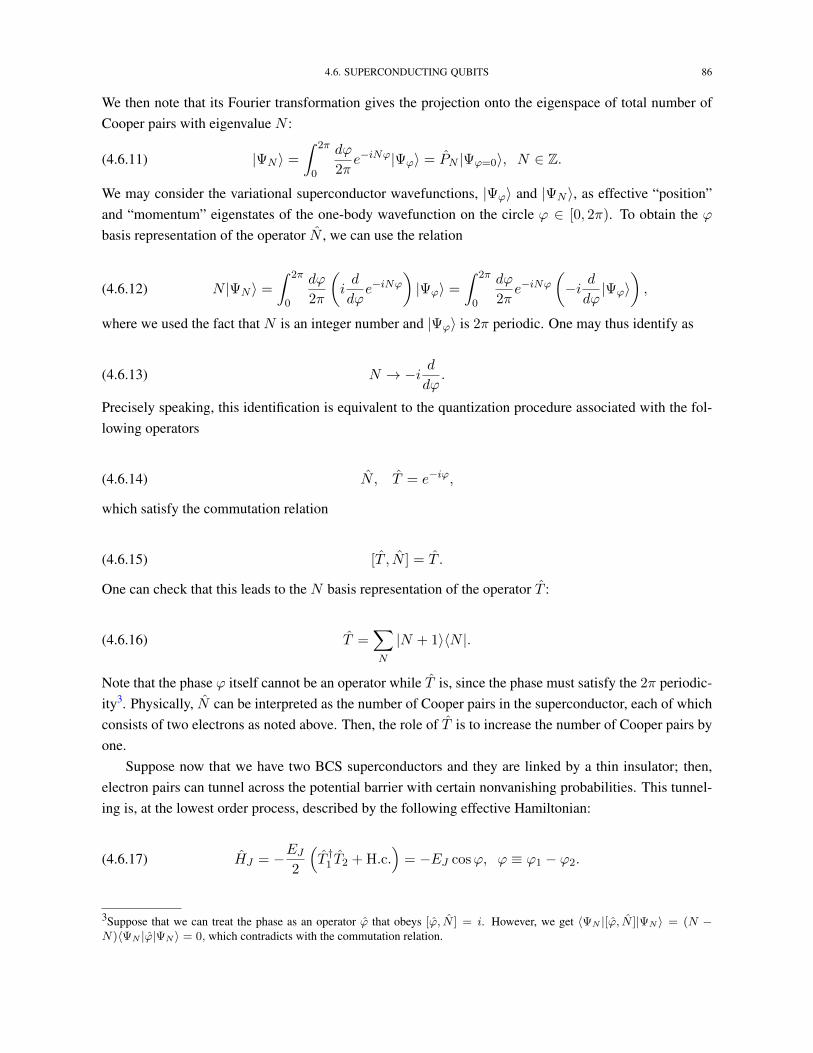
4.6. SUPERCONDUCTING QUBITS 86
We then note that its Fourier transformation gives the projection onto the eigenspace of total number ofCooper pairs with eigenvalue N :
(4.6.11) |ΨN 〉 =
∫ 2π
0
dϕ
2πe−iNϕ|Ψϕ〉 = PN |Ψϕ=0〉, N ∈ Z.
We may consider the variational superconductor wavefunctions, |Ψϕ〉 and |ΨN 〉, as effective “position”and “momentum” eigenstates of the one-body wavefunction on the circle ϕ ∈ [0, 2π). To obtain the ϕbasis representation of the operator N , we can use the relation
(4.6.12) N |ΨN 〉 =
∫ 2π
0
dϕ
2π
(id
dϕe−iNϕ
)|Ψϕ〉 =
∫ 2π
0
dϕ
2πe−iNϕ
(−i ddϕ|Ψϕ〉
),
where we used the fact that N is an integer number and |Ψϕ〉 is 2π periodic. One may thus identify as
(4.6.13) N → −i ddϕ.
Precisely speaking, this identification is equivalent to the quantization procedure associated with the fol-lowing operators
(4.6.14) N , T = e−iϕ,
which satisfy the commutation relation
(4.6.15) [T , N ] = T .
One can check that this leads to the N basis representation of the operator T :
(4.6.16) T =∑N
|N + 1〉〈N |.
Note that the phase ϕ itself cannot be an operator while T is, since the phase must satisfy the 2π periodic-ity3. Physically, N can be interpreted as the number of Cooper pairs in the superconductor, each of whichconsists of two electrons as noted above. Then, the role of T is to increase the number of Cooper pairs byone.
Suppose now that we have two BCS superconductors and they are linked by a thin insulator; then,electron pairs can tunnel across the potential barrier with certain nonvanishing probabilities. This tunnel-ing is, at the lowest order process, described by the following effective Hamiltonian:
(4.6.17) HJ = −EJ2
(T †1 T2 + H.c.
)= −EJ cosϕ, ϕ ≡ ϕ1 − ϕ2.
3Suppose that we can treat the phase as an operator ϕ that obeys [ϕ, N ] = i. However, we get 〈ΨN |[ϕ, N ]|ΨN 〉 = (N −N)〈ΨN |ϕ|ΨN 〉 = 0, which contradicts with the commutation relation.

4.6. SUPERCONDUCTING QUBITS 87
The variable ϕ describes the phase difference between two conductors and we have EJ > 0 which meansthat the phase match is energetically favored. The transfer of the Cooper pairs will also lead to the nonzeroelectric dipole between the superconductors that induces the electrostatic energy, which can be describedby
(4.6.18) HC = 4EC
(N −Ng
)2,
where EC = e2/2C is the capacitance energy with C being the total capacitance of the circuit, the factorof 4 comes from the fact that the Cooper pair has charge 2e, and Ng is the global charge bias in the unitof 2e. The resulting total Hamiltonian of the Josephson junction is
(4.6.19) HJJ = HC + HJ = 4EC
(N −Ng
)2− EJ cosϕ.
To make a comparison with the circuit Hamiltonian discussed before, it is also useful to express HJJ interms of the charge and flux variables as
HJJ =
(Q− 2eNg
)2
2C− EJ cos
(2πΦ
Φ0
),(4.6.20)
Q = 2eN , Φ =Φ0
2πϕ =
~2eϕ,(4.6.21)
which explains the replacement in Eq. (4.6.6).
4.6.3. Superconducting qubits: realizing effectively two-level systems. There are in fact severalways to realize effectively two-level systems (qubits) by operating the Josephson junction in differentparameter regimes. As a first approach, we shall consider the regime in which the charge energy isdominant EC EJ (the so-called Cooper-pair-Box regime). It is then useful to work in the N basis,leading to the Hamiltonian
(4.6.22) HJJ = 4EC
(N −Ng
)2− EJ
2
∑N
(|N〉〈N + 1|+ H.c.) .
At EJ = 0, the energy eigenstates are given by the charge eigenstates |N〉 and the ground and firstexcited states correspond to the ones that provide the two lowest values of (N −Ng)
2. Without Josephsonenergy EJ , this setup merely leads to the equal energy spacing that is unfavorable for the purpose ofrealizing qubits, since the resonant operation inevitably induces the transitions between many differentlevels besides the lowest two levels we are interested in. With the nonlinear term EJ > 0, however,energy levels are now inhomogeneously shifted and the energy degeneracies can be lifted, allowing oneto use the two lowest levels as effective qubits. This type of qubits is known as the charge qubits.
In practice, the charge qubit is sensitive to the environmental voltage noise that comes through thefluctuations of Ng, which ultimately leads to the decoherence. To circumvent this difficulty, one possibleway is to work in another regime EC EJ (the so-called transmon regime). In the language of the

4.6. SUPERCONDUCTING QUBITS 88
one-body wavefunction, this corresponds to the deep potential (or equivalently large mass) that associateswith the small “position” fluctuations 〈ϕ2〉 − 〈ϕ〉2 1. This allows us to treat the phase variable ϕ asan effectively continuous variable without 2π-periodicity restriction. Expanding the cos(ϕ) term, we thenarrive at the effective Hamiltonian,
(4.6.23) HJJ ' 4EC
(N −Ng
)2+
1
2EJ ϕ
2 − 1
4!EJ ϕ
4,
which is equivalent to the weakly anharmonic oscillator. Due to this anharmonicity, the energy degen-eracies are lifted and thus one can use the two lowest energy eigenstates as an effective qubit; a quantumoperation can be performed by using a process that is only resonant to the first excitation energy. Thistype of qubits is known as the transmon qubits.
4.6.4. Light-matter interaction: circuit QED. Finally, we shall briefly mention how superconduct-ing qubits can be electromagnetically coupled to microwave photons. To be concrete, suppose that wecapacitively couple the Josephson junction to the LC circuit discussed at the beginning of this section.The corresponding Hamiltonian can be simply obtained by replacing the (normalized) gate voltage Ng bythat of the LC circuit Ng, resulting in
(4.6.24) H = 4EC
(N − Ng
)2− EJ cosϕ+ ~ωra†a,
where we define
(4.6.25) Ng =CgC
Q
2e=Cg2e
√~ω2C
i(a† − a).
Here, we used Eq. (4.6.3) and Cg is the gate capacitance connecting the Josephson junction with the LCcircuit. While we here discuss the coupling to only a single electromagnetic mode (as realized in cavityresonators), more generally, one can couple the Josephson junction to continuum number of electromag-netic modes by using a certain type of resonators such as waveguides.
These systems offer an ideal platform to study the physics of light-matter interaction, namely, theinteraction between collective excitations of electrons (matter) in the superconductors and quantized mi-crowave photons (light) in the LC circuit. This subfield of quantum optics is often referred to as circuitquantum electrodynamics (QED) together with cavity / waveguide QED; we will give a short introductionfor this topic in the next Chapter.
4.6. SUPERCONDUCTING QUBITS 89
Summary of Chapter 4Section 4.2 Quantization of the electromagnetic field
• The free quantum electromagnetic Hamiltonian is equivalent to a collection of indepen-dent harmonic oscillators with eigenfrequencies ωn, which are determined by solving theHelmholtz equation, (∇2 + ω2/c2)Aω = 0, under certain boundary conditions. The corre-sponding elementary excitation is called photon.• In nonrelativistic quantum electrodynamics, the Coulomb gauge is commonly used and leads
to the unusual commutation relation between the vector potential and electromagnetic fieldswith transverse delta function, which apparently violates the locality. This indicates that thevector potential is not a local observable, but still may influence global property like in theAharanov-Bohm effect.
Section 4.3 Bosonic Gaussian states
• A bosonic quantum many-body state is called Gaussian state when it is completely character-ized by only the correlation functions up to the second-order moment. Time evolution gener-ated by a quadratic bosonic Hamiltonian, such as the free quantum electromagnetic fields, isgiven by a bosonic Gaussian unitary.• When a bosonic Gaussian state is used as a variational ansatz for analyzing weakly interacting
BEC, it naturally incorporates the usual treatment including Bogoliubov or Gross-Pitaevskiitheory.
Section 4.4 Fermionic Gaussian states
• A fermionic Gaussian state is completely characterized by the two-point correlation function.Examples include the Slater determinant and BCS states. Time evolution generated by aquadratic fermionic Hamiltonian is given by a fermionic Gaussian unitary.• A coherent state can be constructed also in fermionic systems and is useful for the purpose of
obtaining several formulas of Gaussian states.
Section 4.5 Variational principle
• Time-dependent variational principle (TDVP) gives an optimal way to approximate the exacttime evolution on the variational manifold at each local time. Variational imaginary timeevolution can be viewed as natural gradient descent on the variational manifold.• When applied to Gaussian variational states, TDVP allows us to derive a set of equations of
motion that can be used to analyze ground-state properties or nonequilibrium dynamics ofmany-body systems.
Section 4.6 Superconducting qubits
• When two BCS superconductors are linked by a thin insulator (Josephson junction), its effec-tive Hamiltonian essentially reduces to that of a single quantum particle subject to periodiccosine potential.• The nonlinear inductance in Josephson junction leads to unequal energy spacing and allows
one to use the two lowest energy eigenstates as effectively two-level systems, qubits. Depend-ing on the parameter regimes, they are often called charge or transmon qubits.
4.7. EXERCISES 90
4.7. Exercises
Exercise 4.1 (Field commutation relations: 1 point). Calculate the following unequal-time com-mutation relations among E and B in free space:
[Eα(r, t), Eβ(r′, t′)](4.7.1)
[Bα(r, t), Bβ(r′, t′)](4.7.2)
[Eα(r, t), Bβ(r′, t′)](4.7.3)
Explain how one can interpret the results in terms of the light cone at |r− r′| = c|t− t′|.
Exercise 4.2 (Single-mode bosonic pure Gaussian state: 1 point). Consider the following single-mode pure bosonic Gaussian state:
(4.7.4) |ψ(φ1, φ2, θ, r)〉 = ei2
(xφ2−pφ1)eiθ4 (x2+p2)e−
ir4
(xp+px)|0〉, φ1,2, θ, r ∈ R.
Derive the expression of the covariance matrix in terms of the real parameters φ1,2, θ, r:
(4.7.5) (Γφ)ξη ≡1
2〈ψ|δφξ, δφη
|ψ〉, δφ = φ− φ, ξ, η ∈ 1, 2 ,
where φ = (x, p)T. Similarly, derive the expression of the characteristic function in terms of φ, θ, r, ξand check the following relation:
(4.7.6) χψ (ξ) ≡ 〈ψ|Dξ|ψ〉 = exp
[−1
8ξTσTΓφσξ +
i
2φTσξ
], ξ ∈ R2.
Exercise 4.3 (McCoy’s formula: 1 point). Show McCoy’s formula for the operators x, p satisfying[x, p] = 2i:
(4.7.7) [xmpn]S =1
2m
m∑l=0
(m
l
)xlpnxm−l = exp
(−i ∂∂x
∂
∂p
)xmpn.
Here, [· · · ]S represents the totally symmetric ordering (for example, [xipj ]S = (xipj + pj xi)/2).
Exercise 4.4 (Bosonic Gaussian states: 2 points).
• Express the Wigner function (4.3.34) as the integral over Nb real variables (cf. Eq. (3.9.4)) [youcan replace the trace Tr[· · · ] by the integral over position variables x and perform the integrationover 2Nb variables ξ].

4.7. EXERCISES 91
• Derive the expression of the overlap between two Bosonic Gaussian states Tr[ρ1ρ2]; you mayuse the following formula for a real, symmetric, positive definite matrix A and real vector v:
(4.7.8)∫RN
dNr e−12rTAr+vTr =
√(2π)N
det(A)e
12vTA−1v.
Show that the obtained formula in particular leads to the simplified expression of the purityTr[ρ2] = 1/
√det(Γφ) of a Bosonic Gaussian state.
Exercise 4.5 (Generalized uncertainty relation: 1 point). Show the generalized uncertainty relationfor a general (i.e., not necessarily Gaussian) density operator ρ of bosons:
(4.7.9) Γφ + iσ ≥ 0,
by using the bosonic commutation relations:
(4.7.10)[φξ, φη
]= 2iσξη, σ ≡ iσy ⊗ INb =
(0 INb−INb 0
).
Here, (Γφ)ξη = 12Tr
[ρδφξ, δφη
]is the covariance matrix of ρ. In particular, when ρ is a bosonic
Gaussian state, show that the condition (4.7.9) is equivalent to the positivity of ρ.
Exercise 4.6 (Fermionic Gaussian states: 2 points). Consider a general multi-mode Fermionic
Gaussian state ρ. Show that its purity is given by Tr[ρ2] =
√det[(
I2Nf − Γ2ψ
)/2]. Show also that
the characteristic function of a Gaussian state (4.4.76) is given by (4.4.77) [you may use the canonicalform (4.4.21) and note the relations ψ2
1,2 = 1 or ξ2 = 0].
Exercise 4.7 (Conservation laws in variational analysis: 1 point). Consider a real-valued varia-tional state. Show that the action variational principle (4.5.18) ensures the energy conservation, but it doesnot in general satisfy the other conservation laws.
Exercise 4.8 (Variational time-evolution equations: 1 point). Derive a set of the variational time-evolution equations (4.5.53) and (4.5.55) for Bosonic Gaussian states [you can follow the same procedureas done for the fermionic case above].

CHAPTER 5
Quantum light-matter interaction
We here introduce a theory of nonrelativistic quantum electrodynamics (QED) by including matterdegrees of freedom in the theory of quantized electromagnetic field introduced in the previous Chapter.We first do this within the Coulomb gauge, and introduce several unitary transformations that are useful,e.g., to introduce simplified effective models or analyze strong light-matter interaction. We briefly mentionthe relevance of these discussions to cavity/waveguide/circuit QED systems that are of current interest inthe fields of quantum optics, quantum information science, and quantum chemistry.
5.1. Classical electrodynamics review
Before developing quantum theory, we shall start from reviewing the theory of classical electrody-namics.
5.1.1. Equations of motion. The dynamics of classical electromagnetic fields interacting with clas-sical charged particles are governed by Maxwell’s equations:
(5.1.1) ∇ ·E =ρ
ε0, ∇ ·B = 0, ∇×E = −∂tB, ∇×B =
1
c2∂tE +
1
ε0c2j.
Here, we represent the charge density, current density, and the particle velocity as follows:
(5.1.2) ρ(r) =∑α
qαδ(r− rα(t)), j(r) =∑α
qαvαδ(r− rα(t)), vα ≡ dtrα.
Each charged particle obeys the equation of motion:
(5.1.3) mαd2t rα = qα [E(rα(t), t) + vα ×B(rα(t), t)] .
From the Helmholtz theorem, we can introduce the vector potential A and the scalar potential φ via
(5.1.4) B = ∇×A, E = −∂tA−∇φ.
We then write down the Lagrangian of the total system by
L =∑α
1
2mα(dtrα)2 +
∫d3r
(ε02
[E2 − c2B2
]+ j ·A− ρφ
)(5.1.5)
=∑α
1
2mα(dtrα)2 +
∫d3r
(ε02
[(∂tA +∇φ)2 − c2 (∇×A)2
]+ j ·A− ρφ
).(5.1.6)
92

5.1. CLASSICAL ELECTRODYNAMICS REVIEW 93
One can check that the Euler-Lagrange equations for generalized coordinates, A, φ, and rα, reproduceMaxwell’s equations (5.1.1) and the equation of motion (5.1.3). At first sight, it might seem that theLagrangian has the following set of dynamical variables:
(5.1.7) A, ∂tA, φ, ∂tφ , rα,vα .
As shown below, in fact this choice of dynamical variables is redundant since they are not independentdegrees of freedom. Thus, the present system is a constrained dynamical system and, to complete thecanonical quantization, we have to carefully identify the correct (nonredundant) dynamical degrees offreedom in this system.
To this end, we introduce the Fourier transformation of arbitrary field variable by
V(r) =
∫d3k
(2π)3Vke
ik·r,(5.1.8)
Vk =
∫d3r V(r)e−ik·r.(5.1.9)
When it is vector-valued, we recall that the Helmholtz theorem allows us to decompose it into transverseand longitudinal parts as
(5.1.10) V(r) = V⊥(r) + V‖(r),
where each component satisfies
∇ ·V⊥(r) = 0 ⇐⇒ k ·V⊥k = 0,(5.1.11)
∇×V‖(r) = 0 ⇐⇒ k×V‖k = 0.(5.1.12)
More specifically, the transverse part can be obtained by using the transverse delta function:
(5.1.13) (V⊥k )i =∑j
(δij −
kikj|k|2
)(Vk)j .
In real space, this can be read as
(5.1.14) (V⊥(r))i =∑j
∫d3r′ δ⊥ij(r− r′)(V(r′))j ,
where δ⊥ij(r) is defined in Eq. (4.2.38).Using these expressions, we can rewrite Maxwell’s equations in the Fourier space as
(5.1.15) E‖k = − iρk
ε0k2k, B
‖k = 0, ik×E⊥k = −∂tB⊥k , ik×B⊥k =
1
c2∂tE
⊥k +
1
ε0c2j⊥k
with

5.1. CLASSICAL ELECTRODYNAMICS REVIEW 94
(5.1.16) ρk =∑α
qα(2π)3
e−ik·rα , jk =∑α
qαvα(2π)3
e−ik·rα .
Note that the longitudinal part of the last equation,∇×B = 1c2∂tE+ 1
ε0c2j, leads to the following equality
(5.1.17) 0 = ∂tE‖k + j
‖k/ε0 ⇐⇒ 0 = ∂tρk + ik · jk,
which merely indicates the charge conservation and does not provide additional constraints. It is now clearthat the correct choice of the independent dynamical degrees of freedom is the one that contributes to theactual time evolution in Eq. (5.1.15), that is,
(5.1.18)
E⊥k ,B⊥k
, rα,vα ,
while the longitudinal fields always obey the constraints E‖k = − iρk
ε0k2 k and B‖k = 0. Said differently,
it suffices to give the initial conditions of the variablesE⊥k ,B
⊥k
, rα,vα for the purpose of fully
predicting the dynamics of the present system; the whole time evolution is then obtained by solving Eqs.(5.1.15) and (5.1.3) with these initial conditions. We remark that, since E⊥k ,B
⊥k obey the first-derivative
time-evolution equation, we don’t need to specify the initial “velocity” of these variables.
5.1.2. Redundancy in the dynamical variables and the Coulomb gauge. As mentioned before,the original Lagrangian appeared to have 8 dynamical variables for electromagnetic degrees of freedom:
(5.1.19) A, ∂tA, φ, ∂tφ .
However, as we have seen at the last part in the previous section, there should be only 4 dynamicalvariables, which correspond to the transverse fields
E⊥k ,B
⊥k
. To proceed with the quantization, we thus
must omit the redundant, extra 4 degrees of freedom from the theory.To do so, we first note that ∂tφ does not appear in any equations of motion and φ can be related to
other variables via the constraint
(5.1.20) φk =1
k2
(ik · ∂tA‖k +
ρk
ε0
),
which follows from the first equality in Eq. (5.1.15). This fact means that ∂tφ and φ are not actualdynamical degrees of freedom, but can be eliminated from the theory through this constraint.
Now there are 6 variables. To identify another constraint, we recall the relations between electromag-netic fields and the potentials in the Fourier space:
(5.1.21) B⊥k = ik×A⊥k , E⊥k = −∂tA⊥, E‖k = −∂tA‖k − ikφk.
Since we know that the variablesE⊥k ,B
⊥k
constitute the independent dynamical degrees of freedom,
we can conclude that it suffices to consider only the transverse component of the vector potential A as

5.1. CLASSICAL ELECTRODYNAMICS REVIEW 95
dynamical variables. This can be achieved most easily by imposing the following gauge condition, whichis known as the Coulomb gauge:
(5.1.22) ∇ ·A(r) = 0 ⇐⇒ A‖(r) = A‖k = 0.
Altogether, we now identify that, in terms of the potentials, the 4 independent dynamical degrees offreedom correspond to the transverse components of the vector potential and their “velocity”:
(5.1.23)
A⊥, ∂tA⊥.
For the sake of notational simplicity, from now on, we shall abbreviate ⊥ in A⊥ and assume that thevector potential is always transverse.
To derive the Hamiltonian, we have to express the Lagrangian in terms of only independent dynamicalvariables A, ∂tA , rα,vα. To this end, we eliminate the longitudinal electric field E‖ and the scalarpotential φ in the original Lagrangian,
(5.1.24) L =∑α
1
2mα(dtrα)2 +
∫d3r
(ε02
[E2 − c2B2
]+ j ·A− ρφ
),
in the following way
∫d3r
(ε02|E‖(r)|2 − ρφ
)= −1
2
∫d3r|∇φ(r)|2 = −VC(5.1.25)
VC ≡1
4πε0
∑α>β
qαqβ|rα − rβ|
,(5.1.26)
which gives the electrostatic contributions. Using the relation
(5.1.27) E⊥ = A, B = ∇×A,
we then arrive at
(5.1.28) L =∑α
1
2mα(dtrα)2 − VC +
∫d3r
(ε02
[(∂tA)2 − c2(∇×A)2
]+ j ·A
).
One can now derive the canonical momentum as
pα ≡∂L
∂(dtrα)= mdtrα + qαA(rα),(5.1.29)
Π ≡ δL
δ(∂tA)= ε0∂tA,(5.1.30)
which leads to the Hamiltonian

5.2. QUANTIZED ELECTRODYNAMICS HAMILTONIANS 96
H =∑α
pα · dtrα +
∫d3rΠ · ∂tA− L(5.1.31)
=∑α
[pα − qαA(rα)]2
2mα+ VC +
∫d3r
[Π2
2ε0+ε0c
2
2(∇×A)2
].(5.1.32)
To simplify the expression, let us assume the periodic boundary conditions and use the mode expansionof A and Π in terms of mode functions fkλ(r) = εkλe
ik·r/√V (cf. Eqs. (4.2.29) and (4.2.19) in Chapter
4):
A(r) =∑kλ
(αkλεkλ
eik·r√V
+ c.c.
),(5.1.33)
Π(r) =∑kλ
(−iε0ωkαkλεkλ
eik·r√V
+ c.c.
)(5.1.34)
with the dispersion relation
(5.1.35) ωk = ck.
Then, the electromagnetic part of the total Hamiltonian can be rewritten as
(5.1.36)∫d3r
[Π2
2ε0+ε0c
2
2(∇×A)2
]=∑kλ
[P 2
kλ
2ε0+ε0ω
2k
2Q2
kλ
],
where we define the generalized coordinates and momentum variables by
(5.1.37) Qkλ ≡ αkλ + α∗kλ, Pkλ ≡ iε0ωk(α∗kλ − αkλ).
5.2. Quantized electrodynamics Hamiltonians
5.2.1. Quantum electrodynamics in the Coulomb gauge. It is now straightforward to quantize theclassical electrodynamic Hamiltonian in the Coulomb gauge obtained above:
HC =∑α
[pα − qαA(rα)]2
2mα+ VC +
∑kλ
[P 2
kλ
2ε0+ε0ω
2k
2Q2
kλ
],(5.2.1)
A(r) =∑kλ
(αkλεkλ
eik·r√V
+ c.c.
).(5.2.2)
Specifically, we require that the particle coordinate and momentum obey the canonical commutation rela-tions
(5.2.3) [(rα)i, (pβ)j ] = i~δαβδij ,
while the same also applies to the generalized coordinates and momentum for electromagnetic degrees offreedom:

5.2. QUANTIZED ELECTRODYNAMICS HAMILTONIANS 97
(5.2.4) [Qkλ, Pk′λ′ ] = i~δkk′δλλ′ .
In terms of normal variables αkλ, the latter is equivalent to the following replacement:
(5.2.5) αkλ →
√~
2ε0ωkakλ
where akλ is the bosonic annihilation operator satisfying the commutation relation:
(5.2.6) [akλ, a†k′λ′ ] = δkk′δλλ′ .
Summarizing, the quantized electrodynamic Hamiltonian is finally given by
(5.2.7) HC =∑α
[pα − qαA(rα)
]2
2mα+ VC +
∑kλ
~ωka†kλakλ
with the vector potential being
(5.2.8) A(r) =∑kλ
√~
2ε0ωkV
(akλεkλe
ik·r + H.c.).
Note that the present formulation in the Coulomb gauge remains valid as far as we are interested inlow-energy behavior in the sense ~ω mc2. To describe high-energy process at ~ω ≥ mc2, such ascreation of electron-positron pairs, we have to treat also matter degrees of freedom as excitations of fieldoperators on equal footing. There, rather than the Coulomb gauge, it is more natural to use the gaugecondition that is manifestly relativistic invariant.
5.2.2. Unitary transformation. One can employ a unitary transformation to analyze the obtainedQED Hamiltonian in another reference of frame other than the Coulomb gauge. The most general formfor such unitary transformation is1
(5.2.9) U = exp
[i
~f(rα, pα ;
akλ, a
†kλ
)],
where f is some function of particle and photon operators, rα, pα andakλ, a
†kλ
. In the transformed
frame, all the observables O (including the Hamiltonian, position operators, field amplitudes, etc) arerelated to the original expressions in the Coulomb gauge via
(5.2.10) ˆO = U †OU ,
while a quantum state is transformed to be
(5.2.11) |Ψ〉 = U †|Ψ〉.
1In principle, one can also include manifestly time-dependent variables, which may be useful when there exists classical externaldrivings.

5.2. QUANTIZED ELECTRODYNAMICS HAMILTONIANS 98
Of course, all the frames must ultimately give the same physical results. In practice, however, one cannotexactly solve the exact QED Hamiltonian and usually resort to a variety of approximations as discussedbelow. After performing such approximations, different references of frames in general lead to differ-ent predictions since the validity of making certain approximations can depend on a choice of frames.This means that some frames may significantly simplify the analysis compared to other frames, and thusit is often crucial how to choose a correct frame of reference depending on different regimes/physicalphenomena at hand.
5.2.3. Gauge transformation. One particular class of unitary transformations corresponds to merelyadding the time-derivative term to the Lagrangian, which is nothing but the gauge transformation. Specif-ically, the corresponding unitary transformation takes the form
(5.2.12) U = exp
[i
~f(rα ; A
)],
which means that f is a function of only generalized coordinates rα and A; the latter means that it includesa, a† operators only through the vector potential A.
To see that this indeed corresponds to the gauge transformation, consider adding the time-derivativeterm to the classical Lagrangian:
L(rα, dtrα ; A, ∂tA) = L(rα, dtrα ; A, ∂tA) +df
dt(5.2.13)
= L(rα, dtrα ; A, ∂tA) +∑α
dtrα∂f
∂rα+ ∂tA
∂f
∂A.(5.2.14)
The new canonical momentum variables are
(5.2.15) pα ≡∂L
∂(dtrα)= mdtrα − eA(rα) +
∂f
∂rα= pα +
∂f
∂rα
and
(5.2.16) Π ≡ δL
δ(∂tA)= ε0∂tA +
∂f
∂A.
The corresponding new Hamiltonian is
H =∑α
pα · dtrα +
∫d3r Π · ∂tA− L(5.2.17)
=∑α
[pα − qαA(rα)]2
2mα+ VC +
∫d3r
[Π2
2ε0+ε0c
2
2(∇×A)2
].(5.2.18)
This means that the form of the Hamiltonian is invariant under the gauge transformation, while one has toreplace the canonical momentum by the transformed ones via
(5.2.19) pα → pα, Π→ Π.

5.3. LONG WAVELENGTH APPROXIMATION 99
It is now clear that, in the language of quantum mechanics, the above unitary transformation (5.2.12)indeed induces such replacement2:
ˆpα = U †pαU = pα +∂f
∂rα(5.2.20)
ˆΠ = U †ΠU = Π +∂f
∂A.(5.2.21)
We note that gauge transformation is just a special subclass among all the possible unitary transforma-tions, and there still exists a much wider class of unitary transformations that do not reduce to the gaugetransformations; we will see such examples later.
5.3. Long wavelength approximation
Consider a globally charge-neutral system (such as a neutral atom) that consists of nuclei and localizedelectrons, whose center of mass is positioned at r = 0. If the dynamics of those particles are well localizedin the length scales that are much shorter than typical wavelengths of photons, we can perform the long-wavelength approximation:
(5.3.1) A(rα) ' A(0).
From now on, we impose this condition and abbreviate the position variable as A ≡ A(0). For the sakeof simplicity, suppose that there is essentially a single valence electron in a neutral system that contributesto the electrodynamics, and its motion around the nuclei can be modeled by using a simplified effectivepotential V (r). We then arrive at the following QED Hamiltonian in the Coulomb gauge:
HC =
[p + eA
]2
2me+ V (r) +
∑kλ
~ωka†kλakλ,(5.3.2)
A =∑kλ
√~
2ε0ωkV(akλεkλ + H.c.) .(5.3.3)
Below we shall illustrate the applications of several unitary transformations to this type of Hamiltoniansunder the long-wavelength approximation.
5.3.1. Power-Zienau-Woolley transformation and dipole interaction. Let us first consider a con-crete example of the gauge transformation known as the Power-Zienau-Woolley (PZW) transformation:
(5.3.4) U = exp
[i
~f(r; A
)], f ≡ −er · A,
2Strictly speaking, the condition (5.2.21) may include redundant degrees of freedom depending on a choice of the gauge con-ditions in the original Hamiltonian. In that case, it must be modified such that it is expressed by only using the independentdynamical degrees of freedom.

5.3. LONG WAVELENGTH APPROXIMATION 100
which transforms the particle momentum as
(5.3.5) ˆp = U †pU = p +∂f
∂r= p− eA.
To determine how the electromagnetic canonical momentum Π changes under this transformation, werecall that in the Coulomb gauge it is related to the transverse electric field via Π = −ε0E⊥. We thusobtain
( ˆE⊥(r))i = U †(E⊥(r))iU(5.3.6)
= (E⊥(r))i +ie
~
[r · A, (E⊥(r))i
](5.3.7)
= (E⊥(r))i +e
ε0
∑j
δ⊥ij(r)(r)j(5.3.8)
where we used the commutation relation (4.2.39). One can check that the magnetic field B remainsinvariant under the transformation. Using the relation
(5.3.9)∑kλ
~ωka†kλakλ + const. =
ε02
∫d3r
[E⊥2(r) + c2B2(r)
],
we then arrive at the transformed Hamiltonian in the PZW gauge:
HPZW = U †HCU(5.3.10)
=p2
2me+ V (r) + er · E⊥ +DP 2(r) +
∑kλ
~ωka†kλakλ,(5.3.11)
where we recall that we abbreviate the position variables in the electromagnetic fields: er · E⊥ ≡ er ·E⊥(0). This r · E term describes the light-matter interaction in this frame, which is called the dipoleinteraction term. There is additional term corresponding to the dipole self-energy:
DP 2(r) ≡ e2
2ε0
∫d3r
∑ijm
rirjδ⊥im(r)δ⊥jm(r).(5.3.12)
=e2
2ε0
∫d3k
(2π)3
∑ijm
rirj
(δim −
kikmk2
)(δjm −
kjkmk2
).(5.3.13)
While this term appears to be divergent, it is in fact nondiverging since we must restrict the k integrationup to a certain momentum cutoff, above which the long wavelength approximation becomes inapplicable.At the cost of introducing the dipole self-energy, we note that the PZW Hamiltonian no longer possessesA2 term that was present in the Coulomb gauge.
5.3.2. Matrix elements in different gauges and TRK sum rule. Since the long wavelength approx-imation should remain valid in both Coulomb and PZW gauges (at least in the weak light-matter couplingregimes), we expect that the different gauges must provide the same physical predictions, despite theapparently different expressions of the Hamiltonians.

5.3. LONG WAVELENGTH APPROXIMATION 101
To explicitly demonstrate this equivalence for one- and two-photon processes, consider an externaldriving by a weak monochromatic classical field at frequency ω:
A(r = 0, t) = Aε cos(ωt)(5.3.14)
E(r = 0, t) = ωAε sin(ωt)(5.3.15)
with ε = (1, 0, 0)T. At the leading order, we can neglect the A2 term in HC and the DP 2 term in HPZW.In the Coulomb gauge, the first-order time-dependent perturbation theory with respect to the interactionterm Hint,C = e
m p ·A in HC leads to the transition amplitude
(5.3.16) S1C = −2πi
~A
2fnmδ(ωnm − ω),
where fnm is
(5.3.17) fnm ≡e
m〈n|p|m〉, p = ε · p,
which includes the matrix elements of the momentum operator between two internal energy eigenstatesof the neutral atom, having an energy difference ~ωnm ≡ En − Em.
In the PZW gauge, the similar perturbation calculation with respect to the interaction term Hint,PZW =
er ·E in HPZW results in the transition amplitude
(5.3.18) S1PZW = −2πi
~A
2fnmδ(ωnm − ω),
where fnm is given by
(5.3.19) fnm ≡ ieω〈n|r|m〉, r = ε · r,
which, in this case, includes the matrix elements of the position operator.We want to check that these two different gauges predict the same transition amplitude, namely,
(5.3.20) S1C = S1PZW ⇐⇒ fnm = fnm.
This equivalence follows from the relation between matrix elements of momentum and position operatorsin the energy basis:
(5.3.21) 〈n|p|m〉 = −im~〈n|[r, H0]|m〉 = imωnm〈n|r|m〉,
where we define the single-particle Hamiltonian by
(5.3.22) H0 =p2
2me+ V (r)
and use H0|n〉 = En|n〉.Similarly, one can also check the gauge equivalence for two-photon transition processes. The second-
order time-dependent perturbation theory in the Coulomb gauge leads to

5.3. LONG WAVELENGTH APPROXIMATION 102
(5.3.23) S2C = −2πi
~
(A
2
)2
gnmδ(ωnm − ω),
where
(5.3.24) gnm ≡( em
)2∑l
〈n|p|l〉〈l|p|m〉ω − ωlm
.
The transition amplitude in the PZW gauge is
(5.3.25) S2PZW = −2πi
~
(A
2
)2
gnmδ(ωnm − ω)
with
(5.3.26) gnm ≡ −ω2e2
~∑l
〈n|r|l〉〈l|r|m〉ω − ωlm
.
One can check that the equivalence between these results,
(5.3.27) S2C = S2PZW ⇐⇒ gnm = gnm,
directly follows from the Thomas-Reiche-Kuhn (TRK) sum rule (see Exercise):
(5.3.28)∑l
(ωln + ωlm) 〈n|r|l〉〈l|r|m〉 =~mδnm.
The TRK sum rule can be shown as follows:
∑l
(ωln + ωlm) 〈n|r|l〉〈l|r|m〉 = − i
m
∑l
(〈n|r|l〉〈l|p|m〉 − 〈n|p|l〉〈l|r|m〉)(5.3.29)
= − i
m〈n|[r, p]|m〉 =
~mδnm,(5.3.30)
where we used Eq. (5.3.21) to obtain the first equality.
5.3.3. Unitary transformations beyond gauge transformations. As noted earlier, there also existunitary transformations that do not reduce to the gauge transformations. Some of them are useful for thepurpose of analyzing quantum light-matter systems in certain regimes; let us briefly look at such examplesbelow.
5.3.3.1. Pauli-Fierz-Kramers transformation. The first example is the Pauli-Fierz-Kramers transfor-mation, by which the light-matter interaction can be absorbed by the field-induced shift of the particleposition together with the fluctuation in the particle potential. To simplify the argument, we consider 1Dcase as follows:

5.3. LONG WAVELENGTH APPROXIMATION 103
HC =
[p+ eA
]2
2me+ V (x) +
∑k
~ωka†kak,(5.3.31)
A =∑k
fk
(ak + a†k
).(5.3.32)
Starting from this Coulomb-gauge Hamiltonian, we define the unitary transformation
(5.3.33) U = exp
(− i~pZ
), Z ≡
∑k
(−ie) fkmeωk
(a†k − ak
),
which includes the particle momentum p, and the field operator Z that does not reduce to A; thus it cannotbe described as a gauge transformation.
The unitary transformation acts on each operator as
U †xU = x+ Z(5.3.34)
U †akU = ak −efk
me~ωkp.(5.3.35)
The coefficients in Z are chosen in such a way that the p · A term in the Coulomb gauge is cancelled bythe term arising from the shift of the a†a term. The resulting transformed Hamiltonian is
HPFK = U †HCU(5.3.36)
=
[1− 2
∑k
e2f2k
me~ωk
]2me
p2 +e2
2me
(A−
∑k
2ef2k
me~ωkp
)2
+ V (x+ Z) +∑k
~ωka†kak(5.3.37)
' 1
2mep2 + V (x+ Z) +
∑k
~ωka†kak,(5.3.38)
where the last expression holds true only for a weak light-matter coupling. An advantage of this expres-sion is that, at the lowest order of e, the light-matter interaction is incorporated only through the potentialterm V , and this feature can simplify calculations of transition amplitudes for certain scattering processes.
5.3.3.2. Asymptotically decoupling transformation. The Pauli-Fierz-Kramers transformation intro-duced above is not very satisfactory in the sense that, at strong light-matter coupling, the higher-orderterms in Eq. (5.3.37) must contribute to dynamics in a rather complicated manner.
To circumvent this difficulty, one can introduce the asymptotically decoupling (AD) unitary trans-formation, which can completely disentangle light and matter degrees of freedom in the strong-couplinglimit. To do so, we first note that one can diagonalize the quadratic photon part in HC as
(5.3.39)e2A
2me+∑k
~ωka†kak =∑n
~Ωnb†nbn + const.
This is always possible by using a certain bosonic Gaussian transformation we studied in the previousChapter. In terms of new photon operators bn, b
†n, one can show that the Hamiltonian takes the following
5.3. LONG WAVELENGTH APPROXIMATION 104
form (see Exercise):
(5.3.40) HC =p2
2me+ V (x)− p
∑n
ζn(bn + b†n) +∑n
~Ωnb†nbn.
We then define the unitary transformation
(5.3.41) U = exp
(− i~pΞ
), Ξ ≡
∑k
iζnΩn
(b†n − bn
),
which again does not reduce to a gauge transformation since it includes the operators p and Ξ 6= A. Thistransformation acts on each operator as
U †xU = x+ Ξ,(5.3.42)
U †bnU = bn +ζn~Ωn
p.(5.3.43)
Note that the coefficients in Ξ are chosen in such a way that, at this time, the interaction term−p∑
n ζn(bn+
b†n) in HC is cancelled by the term arising from the displacement of b†b term. After some calculationswhich we leave to Exercise, the transformed Hamiltonian is given by a very simplified form:
HAD = U †HCU(5.3.44)
=p2
2meff+ V (x+ Ξ) +
∑n
~Ωnb†nbn(5.3.45)
with the mass being renormalized to
(5.3.46) meff ≡ me
(1 + 2
∑k
e2f2k
me~ωk
).
This expression of the Hamiltonian may look similar to the Pauli-Fierz-Kramers form (5.3.38), however,the crucial point is that the present one (5.3.45) is exact and valid for arbitrary light-matter couplingstrengths (as far as the long wavelength approximation is meaningful). As we will revisit later, an advan-tage of this frame is that the effective light-matter coupling strength (characterized by ζn/Ωn) asymptoti-cally vanishes in the strong coupling limit e → ∞. This “asymptotic freedom” can simplify the analysisof strong coupling physics in quantum light-matter systems.
5.3.4. Spontaneous emission: Wigner-Weisskopf theory. We here illustrate an application of non-relativistic QED to yet another elemental process, namely, spontaneous emission of a photon from anexcited atom. Suppose that the emission is induced by the light-matter interaction between an atomicdipole, which can be modeled by an effectively two-level system, and vacuum electromagnetic field infree space. Projecting the PZW-gauge Hamiltonian (5.3.11) onto the two-level manifold, the total Hamil-tonian is obtained by
(5.3.47) HPZW = ~ωa(σz + 1
2
)− σx
∑kλ
(gkakλ + H.c.) +∑kλ
~ωka†kλakλ,

5.3. LONG WAVELENGTH APPROXIMATION 105
where we introduce the coupling strengths and the dipole matrix element by
(5.3.48) gk =
√ωk
2~ε0Vd · εkλeik·r, d ≡ 〈e|(−er)|g〉.
To further simplify the analysis, one can perform the rotating wave approximation and the Born-Markovapproximation, which can be justified when the light-matter interaction is sufficiently weak. The formerleads to the interaction term
(5.3.49) HSE = −
(σ+∑kλ
gkakλ + σ−∑kλ
g∗ka†kλ
),
while the latter allows us to treat the problem of spontaneous emission within the framework of Markov-ian open systems by integrating out the electromagnetic field. Following the general argument given inChapter 3, we obtain the total decay rate (see Eq. (3.7.17)):
Γ = 2∑kλ
∫ ∞0
dτ |gk|2eiωaτ 〈0|ake−iωkτ a†k|0〉(5.3.50)
=
∫ ∞0
2k2dk
π2
ck
2~ε0|d|2
3πδ(ωa − ck)(5.3.51)
=ω3a|d|2
3πε0~c3(5.3.52)
where we assume the isotropic atom
(5.3.53) |d · εkλ|2 =1
3|d|2
and used the relations
(5.3.54)1
V
∑k
→∫
d3k
(2π)3, ωk = ck,
(5.3.55)∫ ∞
0dτei(ωa−ωk)τ = πδ(ωa − ωk) + P.v.
i
ωa − ωk.
The resulting Markovian master equation for the spontaneous emission is (see Eq. (3.7.18))
dρ
dt= − i
~
(Heff ρ− ρH†eff
)+ Γσ−ρσ+,(5.3.56)
Heff ≡ ~ωa(σz + 1
2
)− i~Γ
2σ+σ− = ~
(ωa −
iΓ
2
)(σz + 1
2
).(5.3.57)
If an observer can access information about electromagnetic modes (by, for example, photodetectors)and knows that no photon is emitted, the initial state then evolves under the effective non-HermitianHamiltonian which is characterized by a complex energy ~(ωa − iΓ/2). In contrast, if an observer doesnot know about when a photon is emitted, the correct description is the master equation and the initiallypure state evolves into a mixed density matrix.

5.4. BRIEF INTRODUCTION TO CAVITY/WAVEGUIDE QED 106
To check that the obtained decay rate is indeed small as appropriate for validating the master-equationdescription, we can rewrite
(5.3.58) Γ =4αQEDω
3a|d|2
3c2e2, αQED ≡
e2
4πε0~c' 1
137.
Thus, we have Γ/ωa ∼ αQED(ra/λa)2 1 where ra is the size of the atomic dipole ra = |d|/e and λa
is the wavelength for atomic transition and we used the long-wavelength condition ra/λa 1.
5.4. Brief introduction to Cavity/Waveguide QED
As we have seen in the previous section, the light-matter interaction between a quantum emitter andquantum electromagnetic field in free space is very weak, which ultimately has its origin in the smallnessof the fine structure constant αQED. This can be problematic especially in the fields of quantum infor-mation technologies or quantum optics, since one needs strong light-matter interaction to efficiently andfaithfully operate, convert, and propagate quantum information in-between (artificial) atoms and photons.
One way to circumvent this difficulty is to confine electromagnetic fields into a tiny box, namely,cavity. This confinement effectively enhances the quantum light-matter interaction since the couplingstrength is proportional to 1/
√V with V being the mode volume. The resulting strong quantum light-
matter coupling allows one to study the interaction between atoms and photons in (typically a few) dis-crete electromagnetic modes at the fundamental level of single quanta. This field, which studies quantumelectrodynamics of atoms and photons confined in cavity, is known as cavity QED. More recently, similarstrong coupling is also achieved for (artificial) atoms coupled to photons in continuum modes; this emerg-ing field is coined as waveguide QED, since continuum electromagnetic modes are typically realized incertain waveguide resonators. Below we shall briefly address some of basics in these fields.
5.4.1. Two-level approximation: quantum Rabi model and Dicke model. To introduce a simpli-fied model for describing cavity QED systems, we typically assume that only a single electromagneticmode in a cavity is dominantly coupled to an atomic dipole. We then start from the effective QED Hamil-tonian in the Coulomb gauge:
(5.4.1) HC =
[p+ eA
]2
2me+ V (x) + ~ωca†a, A = f
(a+ a†
),
where f is the mode amplitude depending on the cavity geometry and ωc is the cavity frequency. Astandard choice of a potential V (x) for modeling an atomic dipole is the double well potential,
(5.4.2) V (x) = v
(1− x2
D2
)2
,
which has two degenerate minima at x = ±D; then, it can represent the spectrum of atomic dipole ofsize ' −eD. The two lowest energy levels play the role of the ground and first excited states, and wemay project the Hamiltonian onto such two-level manifold (i.e., the two-level approximation) to furthersimplify the analysis.

5.4. BRIEF INTRODUCTION TO CAVITY/WAVEGUIDE QED 107
For the purpose of performing the two-level approximation, it is advantageous to switch to the PZWgauge:
HPZW = U †HCU ,(5.4.3)
=p2
2me+ V (x) +mg2x2 + ig
√m~ωcx(a† − a) + ~ωca†a,(5.4.4)
where the PZW transformation is given by
(5.4.5) U = e−iexA
~ , g ≡ −ef√
ωcm~
.
While the Coulomb and PZW gauges must provide the same results if no approximation is made, thetwo-level approximation can in fact make differences between them. In other words, the validity of thetwo-level approximation in fact depends on a choice of reference frames. It is now understood that thePZW gauge is well suited for obtaining a two-level description up to the regimes in which the light-matter coupling strength reaches to an order of elementary excitation energies ~ωa,c (known as ultrastrongcoupling regimes).
To derive the two-level model in the PZW gauge, we consider the two lowest levels of the renormalizedsingle-particle Hamiltonian H0 = p2
2me+ V (x) + mg2x2 in Eq .(5.4.4); note that the last term, mg2x2,
represents the dipole self-energy. We denote the two-level manifold of H0 by |g〉, |e〉 and introduce thePauli operators as
(5.4.6) σz = |e〉〈e| − |g〉〈g|, σx = |e〉〈g|+ |g〉〈e|.
Projecting the matter part of HPZW onto this manifold, we obtain the two-level effective model, oftencalled the quantum Rabi model, as follows:
(5.4.7) HRabi =~ωa
2σz + ~λσx
(a† + a
)+ ~ωca†a,
where λ ≡ fωcd/~ with d = 〈e|(−ex)|g〉 and we replaced a→ ia.These arguments can straightforwardly be generalized to the case of N atomic dipoles coupled to a
cavity electromagnetic mode. Specifically, we start from the Coulomb-gauge Hamiltonian
(5.4.8) HC =N∑i=1
[pi + eA
]2
2me+ V (xi)
+ ~ωca†a,
and perform the multi-dipole PZW transformation U = exp[−ie
∑i xiA
~
], after which we project the
transformed Hamiltonian onto the two-level manifold, and obtain

5.4. BRIEF INTRODUCTION TO CAVITY/WAVEGUIDE QED 108
(5.4.9) HDicke =~ωa
2
N∑i=1
σzi + ~λN∑i=1
σxi
(a† + a
)+ ~ωca†a+
~λ2
ωc
(N∑i=1
σxi
)2
.
The last term arises from the dipole self-energy of multiple atoms, which can also be interpreted as thecavity-mediated dipole-dipole coupling. Strictly speaking, this Hamiltonian should be referred to as thegeneralized Dicke model, since the original Dicke model usually refers to the model without the self-energy term. In fact, the original Dicke model eventually becomes invalid at large λ and is known togive rise to qualitatively inaccurate predictions, such as an occurrence of the (equilibrium) superradianttransition at sufficiently large λ (see Exercise).
5.4.2. Rotating wave approximation: Jaynes-Cummings model. Consider a single atomic dipolecoupled to a cavity electromagnetic mode. If the atomic frequency is near resonant and the light-matterinteraction is weak in the sense |ωa − ωc|, λ ωa,c, we can neglect the contributions from the counterrotating terms σ+a† and σ−a in the Rabi model (5.4.7), which are off-resonant and thus rotate rapidly inthe rotating wave frame. This allows us to further simplify the two-level model (5.4.7) as follows:
(5.4.10) HJC =~ωa
2σz + ~λ
(a†σ− + aσ+
)+ ~ωca†a.
This Hamiltonian is known as the Jaynes-Cummings model and has a conserved quantity
(5.4.11) Nex = a†a+σz + 1
2.
The ground state withNex = 0 is unique and given by |g〉|0〉, while other sector at nonzeroNex is spannedby two states |e〉|Nex−1〉 and |g〉|Nex〉. The spectrum is then obtained by just solving the 2×2 eigenvalueproblem. For instance, at the resonant condition ωa = ωc, excitation energies are given by
(5.4.12) ENex,± = Nexωa ± λ√Nex.
The corresponding energy eigenstates hybridize light and matter degrees of freedom and are often calledas dressed states.
The energy splittings 2λ√Nex depend on the excitation number Nex, which have interesting physical
consequences. To see this, consider exciting an atom by a low-photon external pumping at frequency ω.In the limit of λ→ 0, all the transition processes become resonant at ω = ωa. At λ 6= 0, however, the Nex
dependence of energy splittings allow one to choose ω such that only a specific process is resonant. Thus,in the ideal case where the linewidth is sufficiently small compared to λ, one can realize an effectivelynonlinear optical medium. For instance, if one chooses ω = ωa − λ, only a single photon can be excitedsince two (and higher) photon excitation processes are off-resonant and suppressed, leading to effective“photon blockade”.
5.4.3. Strong-coupling physics: asymptotic freedom. The two-level description discussed aboveultimately breaks down when the coupling strength reaches and surpasses elementary excitation energiesωa,c. Physically, this is because at such strong couplings the photon and atoms are strongly entangled and
5.4. BRIEF INTRODUCTION TO CAVITY/WAVEGUIDE QED 109
thus they form hybridized states consisting of superposition of high-lying energy modes in both photonand atomic levels. It is this strong entanglement that invalidates the level truncations necessary to derivethe two-level models.
To circumvent this difficulty, we can perform the asymptotically decoupling unitary transformationthat we introduced in the previous section. To see this, we first rewrite the Coulomb-gauge Hamiltonian(5.4.1) as
HC =p2
2me+ V (x)− g
√~mΩ
p(b+ b†) + ~Ωb†b,(5.4.13)
Ω ≡√ω2c + 2g2,(5.4.14)
where we perform the Bogoliubov transformation b + b† =√
Ω/ωc(a + a†). We then use the unitarytransformation to get
HAD = U †HCU(5.4.15)
=p2
2meff+ V (x+ Ξ) + ~Ωb†b(5.4.16)
where we introduce
meff = me(1 + 2(g/ωc)2), Ξ = iξ(b† − b),(5.4.17)
U = exp
[− ipΞ
~
].(5.4.18)
Here, the length scale ξ characterizes the effective light-matter coupling strength in the transformed frameand defined by
(5.4.19) ξ ≡ g√
~mΩ3
=
√~g2
m(ω2c + 2g2)3/2
.
Note that ξ converges as ξ ∝ g−1/2 → 0 in the strong-coupling limit g ωc. This means that atomsand photons are asymptotically decoupled in the strong coupling regimes. One can then easily studystrong-coupling physics of light-matter systems in this frame, which is otherwise difficult to analyze ingeneral.
5.4.4. Waveguide QED Hamiltonian and Spin-Boson model. We have so far assumed that atomsare coupled to only a single electromagnetic mode. If we couple atoms to electromagnetic modes ofwaveguide resonators instead of cavity, atoms in general couple to continuum electromagnetic modes. Thediscussions above for cavity QED can be extended to the case of such waveguide QED setups possessingmultiple continuum photon modes.
A particularly well-known model in this context is the continuum-mode counterpart of the Rabi model,which is also known as the spin-boson model:

5.4. BRIEF INTRODUCTION TO CAVITY/WAVEGUIDE QED 110
(5.4.20) HSB =~ωa
2σz + σx
∑k
~λk(a† + a
)+∑k
~ωka†a.
The spin-boson model has historically been extensively studied in the context of open quantum systems,as it can describe dissipative dynamics of a spin-1/2 coupled to bosonic baths. Unless λk is sufficientlyweak, the master equation approach is in general insufficient and thus this model belongs to a class ofnon-Markovian (or nonperturbative) open quantum systems. It is interesting to note that its ground statecan exhibit the quantum phase transition of the Berezinskii-Kosterlitz-Thouless (BKT) type. Under cer-tain conditions, this transition can be identified as the antiferromagnetic-to-ferromagnetic transition in theanisotropic Kondo model. However, to apply the spin-boson description to waveguide QED systems, wehave to keep in mind that this two-level description can be a good effective model only when a number ofassumptions used above are plausible. When some of those assumptions (such as the two-level approxi-mation etc) break down (which might be the case especially at strong light-matter couplings), we have togo back to the original QED Hamiltonian and reexamine the validity of the analysis.
5.4.5. Circuit realizations. As we briefly mentioned in the previous Chapter, one can use supercon-ducting circuits to study the physics of quantum light-matter interaction; this field is often coined as circuitQED. To complete the analogy between circuit QED and cavity QED, let us recall the Hamiltonians ineach case:
Hcircuit = 4EC
(N − Ng
)2− EJ cosϕ+ ~ωra†a, Ng ∝ a† + a,(5.4.21)
Hcavity =
[p+ eA
]2
2me+ V (x) + ~ωca†a, A ∝ a+ a†.(5.4.22)
It is now clear that these two models are essentially equivalent if we identify the potential in the cavityQED Hamiltonian as the periodic potential V (x) ∝ cos(2πx/λ).
In circuit QED, the Josephson junction plays the role of an artificial atom which is coupled to mi-crowave photons in LC circuit. If we couple a Josephson junction to a more complex circuit with infinitelength, this artificial atom will interact with continuum of microwave photons, thus offering an ideal plat-form to study physics of waveguide QED3. Owing to low frequency of photons in circuit setups (typicallyin microwave regimes), it is usually easier to attain strong light-matter couplings in circuit setups thanconventional cavity QED setups (typically in optical regimes). Circuit QED systems are thus also one ofthe most ideal experimental platforms for exploring physics of strong quantum light-matter interaction.
3Strictly speaking, the analogy with the waveguide QED Hamiltonian may not be perfect in this case, since the A2 may in facttake a slightly different form depending on circuit geometry in circuit QED Hamiltonian.

5.4. BRIEF INTRODUCTION TO CAVITY/WAVEGUIDE QED 111
Summary of Chapter 5Section 5.1-5.3 Quantum electrodynamics in the Coulomb gauge and unitary transformations
• To eliminate the redundant degrees of freedom, one can impose the Coulomb gauge condi-tion, after which the standard canonical quantization procedure allows us to obtain the QEDHamiltonian (5.2.7).• The unitary transformation that only includes the particle positions rα and the vector potential
A generates a gauge transformation. One example is the Power-Zienau-Woolley transforma-tion, after which the interaction is described by the r ·E term at the leading order.• There also exist unitary transformations that go beyond gauge transformations. Examples
include the Pauli-Fierz-Kramers or asymptotically decoupling transformations, which can beparticularly useful in strong light-matter coupling regimes.
Section 5.4 Brief introduction to cavity/waveguide QED
• If a dipole is dominantly coupled to only a single electromagnetic mode, we can use the two-level effective model called the quantum Rabi model. This model can be faithfully derivedfrom the QED Hamiltonian in the PZW gauge up to ultrastrong coupling regimes. Its N -dipole generalization gives the (generalized) Dicke model.• When the rotating wave approximation is valid, one can further simplify the model to the
Jaynes-Cummings Hamiltonian.• A single two-level system coupled to continuum electromagnetic modes can be modeled by
the spin-boson model.• When light-matter coupling strength reaches/surpasses energy scales of elementary excita-
tions, both the two-level and rotating wave approximations break down in general. In suchregimes, one may use the asymptotically decoupling transformation to simplify the analysis.

5.5. EXERCISES 112
5.5. Exercises
Exercise 5.1 (PZW gauge without long-wave approximation: 2 points). Introduce the atomic po-larization density by
(5.5.1) P(r) ≡ −er∫ 1
0du δ(r− ur).
Consider the gauge transformation (called the PZW transformation) corresponding to the following uni-tary operator:
(5.5.2) U = exp
[i
~
∫d3r P(r) · A(r)
].
Check that this reduces to Eq. (5.3.4) after performing the long-wave approximation.We here aim to derive the transformed Hamiltonian without resorting to the long-wave approximation.
To do so, consider the exact Coulomb-gauge Hamiltonian
(5.5.3) HC =
[p + eA(r)
]2
2me+ V (r) +
∑kλ
~ωka†kλakλ,
with
(5.5.4) A(r) =∑kλ
√~
2ε0ωkV
(akλεkλe
ik·r + H.c.).
Show that the PZW transformation above leads to the following transformed Hamiltonian:
HPZW = U †HCU(5.5.5)
=
(p− er×
∫ 10 duuB(ur)
)2
2me+ V (r)−
∫d3r P⊥(r) · E⊥(r)
+1
2ε0
∫d3r P⊥2(r) +
∑kλ
~ωka†kλakλ.(5.5.6)
You may use the relations
∑kλ
~ωka†kλakλ + const. =
ε02
∫d3r
[E⊥2(r) + c2B2(r)
],(5.5.7)
[Aα(r, t),−ε0Eβ(r′, t)] = i~δ⊥αβ(r− r′).(5.5.8)

5.5. EXERCISES 113
Exercise 5.2 (Applications of TRK sum rule: 2 points). (a) Show the equivalence between expres-sions of matrix elements for two-photon scattering process in different gauges:
(5.5.9) gnm = gnm
where
(5.5.10) gnm ≡( em
)2∑l
〈n|p|l〉〈l|p|m〉ω − ωlm
, gnm ≡ −ω2e2
~∑l
〈n|r|l〉〈l|r|m〉ω − ωlm
.
You may use the TRK sum rule:
(5.5.11)∑l
(ωln + ωlm) 〈n|r|l〉〈l|r|m〉 =~mδnm.
(b) Consider the Dicke model (5.4.9) at large, but finite number N of electric dipoles. Use the TRK sumrule to show that the energy difference between the first excited state and the ground state does not vanishat any finite light-matter coupling strength4. What would happen if the last term (self-energy term) in Eq.(5.4.9) is neglected? You may use the Holstein-Primakoff approximation:
(5.5.12)N∑i=1
σ+i '
√Nb†,
N∑i=1
σz ' −N + 2b†b,
where b, b† are bosonic operators obeying [b, b†] = 1.
Exercise 5.3 (Mass renormalization in the asymptotically decoupled frame: 2 points). Considerthe Coulomb-gauge Hamiltonian in the long-wave approximation:
HC =
[p+ eA
]2
2me+ V (x) +
∑k
~ωka†kak,(5.5.13)
A =∑k
fk
(ak + a†k
).(5.5.14)
(a) The quadratic photon part can be diagonalized as
(5.5.15)e2A
2me+∑k
~ωka†kak =∑n
~Ωnb†nbn + const.
via the canonical transformation
(5.5.16) ak =∑n
(O)kn
[cosh(rnk)bn − sinh(rnk)b
†n
],
4This argument essentially forbids realization of the equilibrium superradiant transition in cavity QED systems with a singleelectromagnetic mode, which is often called “no-go theorem”. Note, however, that possibility of realizing superradiant transitionis not excluded in general multi-mode cases.

5.5. EXERCISES 114
where rnk ∈ R are squeezing parameters while O is an orthogonal matrix. Determine the expression ofrnk and derive the relation satisfied by O.
(b) In terms of b operators, the Hamiltonian can be written as
(5.5.17) HC =p2
2me+ V (x)− p
∑n
ζn(bn + b†n) +∑n
~Ωnb†nbn.
Determine the expression of ζn by using O. Using the relation derived in (a), show the following relation
(5.5.18)1
1− 2∑
nmeζ2
n~Ωn
= 1 + 2∑k
e2f2k
me~ωk.
Check that this relation leads to the simplified expression of the mass renormalization in meff of theAD-frame Hamiltonian:
(5.5.19) HAD = U †HCU =p2
2meff+ V (x+ Ξ) +
∑n
~Ωnb†nbn
where
(5.5.20) U = exp
(− i~pΞ
), Ξ ≡
∑k
iζnΩn
(b†n − bn
)and
(5.5.21) meff = me
(1 + 2
∑k
e2f2k
me~ωk
).
Exercise 5.4 (Spontaneous emission: 1 point). Consider the isotropic two-level atom coupled tovacuum electromagnetic field. Derive the formula (5.3.52) of the spontaneous emission rate from Fermi’sgolden rule.

CHAPTER 6
Machine learning and quantum science
6.1. Introduction
The field of machine learning, especially artificial neural networks, has witnessed remarkable devel-opments in recent years, and is revolutionizing science and technology. Deep neural networks are nowroutinely applied to classify or recognize patterns/images, translate sentences or speech between differ-ent languages, predict traffic or market trading, and to attain self-driving cars, device/robot controls, andsuperhuman performance in table/video games. In the context of physical science (especially quantumscience), the idea of machine learning has also led to many interesting developments in these years. In thenext two Chapters, we try to give brief and introductory descriptions about some of key concepts/topics inthis rapidly growing field.
In machine learning, there are mainly three classes of problems, namely, supervised, unsupervised,and reinforcement learning. Supervised learning handles data consisting of a pair of vectors xi,yini=1
with y being often called a label and n being the number of data. The goal of supervised learning isto estimate a function f that relates these two vectors via y = f(x). We call it as “supervised” sincethe correct answer (i.e., label) yi is given for each xi by “teacher”, and machine is trained by “teacher”according to this dataset. In contrast, unsupervised learning deals with data that only contains some setof vectors xini=1 that is supposed to be randomly generated by a certain probability distribution p(x).Typically, unsupervised learning aims to either extract essential features/structures behind the data oreven (approximately) construct the distribution p(x) itself by using some tractable ansatz. Since there isno “teacher” who tells us the label, it is called “unsupervised”.
In these two classes of learning problems, the trained machine can at most reproduce or imitate theways that are taught or predicted by the original dataset; machines thus cannot have sort of creativity, inthe sense that they would neither realize performance beyond the teacher nor predict something new thatis not expected from the dataset.
Roughly speaking, reinforcement learning aims to train machines to acquire that sort of creativity forachieving better performance by repeating a huge number of trials and errors. In reinforcement learning,data is not given in advance in contrast to supervised/unsupervised learning, but machine itself acquiresknowledge about data to find the best solution by interacting with an environment. Each solution asso-ciates with some figure of merit called “reward”, and on the basis of its value, the machine tries to search abetter solution from the repetitions of trials and errors. In this sense, there is a feedback loop between themachine (also called agent) and environment, and in fact its theoretical framework fits well with theory ofopen quantum systems (or more specifically, continuous quantum measurement) as we discuss later.
115
6.2. BASIC CONCEPTS 116
Below we begin by introducing some basic concepts of machine learning and black-box optimizations.Building on these understandings, in the next Chapter, we proceed to learn about (deep) reinforcementlearning.
6.2. Basic concepts
6.2.1. Supervised learning.6.2.1.1. Function approximation, cost function, and training. As noted above, the goal of supervised
learning is to identify a function approximation f that relates inputs x to outputs y. We do this byhypothesizing a certain functional form fθ parameterized by θ:
(6.2.1) y = fθ(x).
Given a training dataset xi,yini=1 , we then try to optimize θ in such a way that the resulting fθ imitatesthe training dataset best.
To do so, we have to quantify how well the obtained function fθ reproduces the training dataset. Forthis purpose, we introduce the cost function that usually decomposes into the sum of each data:
(6.2.2) L(θ) =1
n
n∑i=1
λ(xi,yi; θ).
One common way is to use the mean squared error as the cost function:
(6.2.3) L(θ) =1
n
n∑i=1
|yi − fθ(xi)|2 ,
while the specific form of the cost function in general changes depending on type of the problem or achoice of fθ.
After specifying the cost function, we next have to specify how in practice we attempt to find theoptimal θ∗ that would minimize L(θ). A process of finding the optimal values θ∗ is commonly referredto as training, and the most common way for this is to simply apply the gradient descent method. Recallthat we have already encountered the similar idea in the context of imaginary-time evolution of variationalstates in Chapter 4. At each time step, the gradient descent updates the parameters according to
(6.2.4) θτ+δτ = θτ − η∇θL,
where η is some positive and small quantity, often called the learning rate. This means that we changethe parameters along the negative gradient of the cost function. In practice, however, it often takes toomuch time to evaluate L by using all the possible training data. This difficulty can be circumvented byrestricting the ensemble average in L to only a small subset of data called mini batch:
(6.2.5) θτ+δτ = θτ − η∇θLbatch, Lbatch =1
nbatch
nbatch∑i=1
|yi − fθ(xi)|2

6.2. BASIC CONCEPTS 117
with nbatch < n. This is often referred to as stochastic gradient descent in the sense that we use an ap-proximation of the negative gradient, which brings certain noise compared to the “exact” gradient descentcalculated from all the possible data. As we mentioned in Chapter 4, from a geometrical point of view,the gradient descent may be considered as the discrete-time version of the imaginary time evolution onthe variational manifold spanned by fθ.
It is important to note that the choice of a functional ansatz fθ is crucial in supervised learning, butits exact form is unknown a priori in most of practical problems. So, on what basis can we specify suchansatz? A possible guiding principle for this is actually similar to the spirit of variational approach wediscussed in Chapter 4. Specifically, we shall choose a functional ansatz that is (1) flexible, i.e., its repre-sentation capacity is large enough such that it can fit well with reasonably different patterns in practicalproblems (2) tractable and efficient, i.e., there is some efficient algorithm to optimize θ within a reason-able amount of time and numerical computing resource, and (3) scalable, i.e., it can easily be scaled upto handle high-dimensional data. Below we briefly discuss several illustrative examples in supervisedlearning.
Example 1: Kernel method, support vector machine, and variational quantum circuits. Suppose thatwe have dataset xi, yini=1. The kernel method aims to predict output y ∈ R for a given input x ∈ Rm
by using the functional form,
(6.2.6) y =
n∑i=1
αik(x,xi),
where αi are parameters of this model and k is a certain fixed (nonlinear) function called kernel. Oneof the most common choice is to use the Gaussian kernel
(6.2.7) k(x,x′) = exp(−β∣∣x− x′
∣∣2) .In this choice, the kernel method tries to fit the data by using a linear superposition of many Gaussianfunctions as in Eq. (6.2.6).
The cost function is typically given by the mean squared error
(6.2.8) L(α) =1
n
n∑i=1
∣∣∣∣∣∣yi −n∑j=1
αjk(xi,xj)
∣∣∣∣∣∣2
+ σ2n∑
ij=1
αik(xi,xj)αj ,
where the last term is the regularization term that is introduced to avoid the overfitting or divergence ofthe parameters αi.
In fact, in the present problem, we can analytically identify the optimal α∗ that minimizes the costfunction (see Exercise):
(6.2.9) α∗i =
n∑j=1
(K + σ2I
)−1
ijyj ,

6.2. BASIC CONCEPTS 118
where I is the n× n identity matrix and we define the kernel matrix by
(6.2.10) (K)ij = k(xi,xj).
The resulting trained function is
(6.2.11) y =n∑i=1
α∗i k(x,xi) =n∑
ij=1
k(x,xi)(K + σ2I
)−1
ijyj .
This allows us to estimate output y for a given unknown input x.It is worthwhile to note that the kernel method also gives a functional ansatz of the so-called support
vector machine. Consider a binary classification problem with output y ∈ −1, 1. For a given inputx, the support vector machine predicts which class the input vector belongs to, i.e., it gives a positive(negative) class if the function takes a positive (negative) value:
(6.2.12) y = sign
(n∑i=1
α∗i k(x,xi) + b∗
)∈ −1, 1 ,
where we introduce a bias parameter b. In practice, the optimized vector α∗ may have mostly zero com-ponents. One can then simplify the evaluation of the function by restricting the summation over only fordataset that have nonzero α∗i , rather than over all the possible data.
We also note that, in fact, the kernel method has a close connection with some type of quantummachine learning algorithms. In the context of quantum machine learning, one typically encodes an inputvector x into a quantum state |ψ(x)〉. One can then introduce the kernel function by using the innerproduct between two different quantum states by
(6.2.13) k(x,x′) =∣∣〈ψ(x)|ψ(x′)〉
∣∣2 ,and use the function ansatz y =
∑ni=1 αik(x,xi) in the same manner as above, but at this time the kernel
function is evaluated from the overlap of quantum states.A specific form of the kernel depends on type of available quantum computer and how one encodes
the information into a quantum state. As a simple example, let us first consider a harmonic oscillator andsuppose that input data is encoded by a displacement operator
(6.2.14) |ψ(x)〉 = D(x)|0〉 = ex(a†−a)|0〉 ≡ |x〉.
For high-dimensional input data, we consider
(6.2.15) |ψ(x)〉 ≡∏i
|ψ(xi)〉.
Then, the kernel actually corresponds to the usual Gaussian kernal:
(6.2.16) k(x,x′) =∣∣〈ψ(x)|ψ(x′)〉
∣∣2 = exp(−∣∣x− x′
∣∣2) .

6.2. BASIC CONCEPTS 119
Experimentally, this choice would be relevant to photonic quantum computers in which a harmonic oscil-lator represents each electromagnetic mode.
Let us next consider a two-level system and its encoding:
|ψ(x)〉 = exp
(− i
2xσx
)| ↑z〉 = cos
(x2
)| ↑z〉 − i sin
(x2
)| ↓z〉(6.2.17)
|ψ(x)〉 ≡∏i
|ψ(xi)〉.(6.2.18)
This corresponds to the following kernel function
(6.2.19) k(x,x′) =∣∣〈ψ(x)|ψ(x′)〉
∣∣2 =∏i
cos2
(xi − x′i
2
).
This situation should be relevant to a quantum computer consisting of, e.g., the superconducting qubitswe explained in Chapter 4. One can then use these kernel functions (which can be evaluated on a quantumcomputer) as a functional ansatz to fit real-life data. Very roughly speaking, the idea along this line can beconsidered as one of what has been envisioned in the emerging field of quantum machine learning.
In practice, numerical cost of the kernel method is mainly set by the cost of calculating the inversematrix
(K + σ2I
)−1, which basically scales as O(n3) with n being the number of training data. Even iftraining has been performed in some way, the function evaluation requires the summation over dataset andits cost scales linear with n. Thus, the kernel method can in general be applied to a problem with rathermodest size of data, such as n ≤ O(103). This limitation will become a major difficulty when we haveto deal with a large dataset, namely, “big data”. A possible solution for this is to introduce supervisedlearning using deep neural networks, as we briefly discuss next.
Example 2: Neural network and classifying phases of matter. Deep learning basically uses the fol-lowing multilayer feed-forward neural network as a nonlinear functional ansatz fθ:
(6.2.20) fθ(x) = g(wL · · · g(w2 g(w1x))),
where x is the input vector, wi are weight matrices that map input vector at each layer i to another vectorthat becomes an input vector to the next layer, and g is some nonlinear function called activation function.Typical choices for g are
(6.2.21) gsigmoid(x) =1
1 + e−x, gReLU(x) =
x x ≥ 0
0 x < 0,
where ReLU stands for the Rectified Linear Unit function. One may also introduce the bias vector andconsider the affine transformation wix + b. Although it is not the purpose of this course to explain aboutdetails of deep learning, we here remark that there is an efficient and simple algorithm (based on thestochastic gradient descent and chain-rule calculations of derivatives) to train this function in a reasonable

6.2. BASIC CONCEPTS 120
amount of time even for vastly large dataset. From empirical success of deep learning, we know that thetrained function fθ∗ found by this algorithm would fit well training data set and, surprisingly, somehowgeneralizes well (i.e., it can predict well for unknown input). Interestingly, this seems to be the case whenthe network is deep and has many layers, for which the function appears to be overparametrized. Currently,it is a commonly held view that there is still little theoretical understanding behind this unreasonablesuccess of deep learning.
One of the most well-known applications of the multilayer feed-forward neural network (or precisely,so-called convolutional neural network) is the problem of image classification. It basically gets 2D imageas an input data and predicts which class that image belongs to, say, cat or dog. In the context of physics,the success of deep learning in this problem inspires physicists to apply it to the problem of classifyingphases of matter. From a close analogy with the variational approach in quantum many-body physics,deep neural networks also motivate quantum physicists to use them as variational ansatz for quantummany-body wavefunctions, as we briefly discuss later. Interested students may refer to, for example, [Rev.Mod. Phys. 91, 045002 (2019)].
6.2.2. Unsupervised learning. In unsupervised learning, we deal with data xini=1 without labelsand typically aim to extract essential information about the probability distribution that generates trainingdataset. In some cases, one attempts to directly construct the probability distribution itself by using acertain functional ansatz and optimizing it to find the best approximations of the distribution. There aremany different ways for doing this, but here let us only mention two of the most well-known examples.
Example 3: Autoencoder. Suppose that we have dataset which should possess certain structure, butwe do not know what structure it specifically represents since the data has no labels; one may imagine,for instance, a set of 2D images of animals for some unknown different species. How can one identifythe possible structure behind the data? The idea of autoencoder is to use neural networks to extract keyfeatures of dataset by compressing the original data into a much smaller vector space, but without loosingessential information. Specifically, it attempts to reproduce its input vector itself as output vector:
(6.2.22) x ' fθ(x)
by optimizing θ in neural networks whose middle layers have much fewer neurons than those in the in-put/output layers. In this way, at the middle layers, data is significantly compressed and lives in muchsmaller vector space, while hopefully this compression can be done without loosing too much informationabout data, i.e., keeping the most relevant features of the input data. The intuition behind this is that (aslong as the learning is successful) the trained network is supposed to reconstruct the input data only fromthe limited amount of information encoded in the restricted middle layer. The neurons in this middle layeris often called latent variables, since they represent the relevant features of input data which are a prioriunknown. The philosophy behind autoencoder may fit well with physics, namely, the idea that there mustexist only a few key principles behind data generated from the laws of physics that we want to understand;naturally, autoencoder has already found many applications in physical science.

6.2. BASIC CONCEPTS 121
Example 4: Restricted Boltzmann machine and neural network states. Suppose that dataset xini=1
is generated by some unknown probability distribution p(x). We want to construct a model that imitatesthis distribution by using a flexible, efficient, and scalable variational ansatz pθ(x). In practice, we donot know the exact form of a true distribution p(x), but can access about the empirical “data” distributionpData(x) that gives its approximation:
(6.2.23) pData(x) =1
n
n∑i=1
δx,xi .
The most common way for the optimization, i.e., training of the model pθ(x), is to use the cross entropy
(6.2.24) L(θ) = −∑x
pData(x) ln pθ(x) = − 1
n
n∑i=1
ln pθ(xi).
We can rewrite it (aside constant) by
(6.2.25) L(θ) = D [pData(x)||pθ(x)] + const.,
where we define the relative entropy for given probability distributions p, q via
(6.2.26) D [p(x)||q(x)] ≡∑x
p(x) lnp(x)
q(x).
The relative entropy vanishes D = 0 if and only if the two distributions coincide, i.e., p(x) = q(x) for∀x. Roughly speaking, the relative entropy thus quantifies how much there is difference between twodistributions. The minimization of the cost function above then corresponds to the process that makes themodel pθ similar to the empirical distribution pData as much as possible.
The restricted Boltzmann machine (RBM) is one example of possible variational ansatz pθ, which isdefined by
pθ(v) =∑h
pθ(v,h) ≡∑h
e−Eθ(v,h)
Z,(6.2.27)
Eθ(v,h) ≡ −a · v − b · h− vTWh, Z ≡∑v,h
e−Eθ(v,h).(6.2.28)
where v are actual variables for representing data and called “visible” units, while the “hidden” units h
are summed over before giving the model and do not appear in pθ(v). These units are typically binaryvariables vi, hi ∈ 0, 1. The model parameters θ include real vectors a,b and matrix W ; we emphasizethat there are no direct couplings among hidden variables h and also among v. This particular structure ofthe couplings is the reason for calling this model “restricted” since the coupling network of v,h can thenbe represented by the connection between the single hidden layer and the visible layer.
An apparent difficulty in this variational ansatz is that it is computationally intractable to perform thesummation over exponentially large number of configurations for v and h in the partition function Z andthus to evaluate pθ(v). That said, it is noteworthy that one can still efficiently evaluate the conditional
6.3. BLACK-BOX OPTIMIZATION 122
distribution as follows:
(6.2.29) pθ(h|v) ≡ pθ(v,h)
pθ(v)=∏i
ezihi
1 + ezihi, z ≡ b +Wv.
A similar expression can be obtained for pθ(v|h). This fact simplifies the calculation of the gradient ofthe loss function ∇θL to some extent, but the computational difficulty of Z itself is unavoidable anyway.We mention that there are still several heuristic approaches to tackle this difficulty, such as the methodso-called contrastive divergence.
In the context of quantum many-body physics, the RBM inspires physicists to introduce the followingvariational many-body states often called neural network states1 [Science 355, 602 (2017)]:
|ΨRBM〉 =∑σ
Ψσ|σ〉(6.2.30)
Ψσ ≡1
Z
∑h
exp[a · σ + b · h + σTWh
].(6.2.31)
whereσ ∈ 0, 1n are binary variables representing spin-1/2 states and |σ〉 corresponds to the basis states.It is known that any many-body state can then be arbitrarily well approximated by an RBM state if thenumber of hidden units is larger than the number of configurations |σ〉 satisfying |Ψσ| > 0. Intuitively,one may say that the correlations of physical variables σ are effectively induced by hidden variables h andthey can be nonlocal if the coupling W is long-ranged2. In practice, to find the optimal RBM variationalstate for, e.g., the ground state of some many-body Hamiltonian, one can use the stochastic gradientdescent and standard techniques which are common in variational Monte Carlo method.
6.3. Black-box optimization
To minimize a cost function, one has to choose some optimization algorithms. As introduced above,the most elemental way for this is to use the (stochastic) gradient descent. In Chapter 4, we have also men-tioned that one can improve this method and use the so-called natural gradient descent when the geometryof the variational manifold is appropriately taken into account. From a broader perspective, there existother types of optimization methods that do not rely on the local gradient as used in the aforementionedexamples, but on some heuristic algorithms, some of which are inspired by ecology. These methods areheuristic in the sense that they usually lack solid theoretical justifications, while are empirically known tobe effective in many challenging optimization problems.
We here cover several examples of such heuristic optimization algorithms, also known as black-boxoptimizations. In this approach, to optimize the objective (that is not in a solvable, closed form function)with respect to parameters θ, we do not need to calculate its derivative or even require the differentiability,but use the value of the fitness function F (θ), which gives a certain measure about the optimality of a
1Precisely speaking, neural network states often refer to a slightly generalized version of the RBM states, in the sense that thenetwork structure of physical σ and hidden h variables is not necessarily restricted to the bipartite graph with a single hiddenlayer as in RBM.2If couplings W are short-ranged or sparse, one can show that the RBM states have only small entanglement, i.e., they obey thearea law, and thus can be efficiently represented by the matrix product states.

6.3. BLACK-BOX OPTIMIZATION 123
Algorithm 1 Random search1: Initialize: θ2: while till convergence of F do3: Get: fitness value F (θ)4: Sample a new parameter set θnew from θ5: if F (θnew) > F (θ) then6: θ ← θnew
solution. This fitness function may be the objective function itself, but needs not to be so. While thegradient-based optimization methods tend to be trapped in local minima, black-box optimizations aregradient-free and can often circumvent this difficulty; this is the reason why black-box optimizations areoften also referred to as global search methods. Below we assume that the optimization problems isformulated in such a way that the goal is to maximize the fitness function (which is consistent with theusual convention in the literature).
Random search. The simplest example of black-box optimization would be the random search.Firstly, it randomly chooses an initial value θ0 and calculates the fitness F (θ0). We then stochasticallygenerate a new set of parameters θnew
0 starting from θ0 by using some given probability distribution. Cal-culating the fitness F (θnew
0 ) for this parameter set, and if the new one is better than the old one, i.e.,F (θnew
0 ) > F (θ0), we accept the change and set the parameters at the next step as θ1 = θnew0 , otherwise
we set θ1 = θ0. This procedure will be repeated many times until the convergence of the fitness. As aprobability distribution for selecting a new candidate parameter θnew
t from θt, we typically use the uni-form distribution over the hypersphere with a fixed radius centered at θt. The algorithm is summarized inAlgorithm 1.
Evolutionary strategy. A major difficulty in random search is its low sample efficiency; it literallysearches the whole parameter space randomly and it often fails or takes too much time to finally reach thecorrect optimal solution. In this context, the evolutionary strategies refer to methods that aim to improvethe search efficiency by developing a heuristic algorithm inspired by the evolution process. While there aremany variants of evolutionary strategies, here we consider one concrete example, known as the covariancematrix adaptation evolution strategy (CMA-ES).
The algorithm of the CMA-ES is summarized in Algorithm 2. The key point is that we use a minibatchof random vectors εini=1 and use the averaged fitness 1
n
∑ni=1 εiFi as a (finite step) differential direction
at the next generation. In this sense, one can say that this algorithm is in the similar spirit of the gradientdescent algorithms, but the advantage here is that one does not need to explicitly calculate the derivativeor even assume the differentiability of the fitness function. While we here discuss the simplest CMA-ES
Algorithm 2 CMA-ES1: Initialize: θ, η, σ2: while till convergence of F do3: Sample n random vectors εini=1, each component sampled from N (0, 1)4: Get: fitness values Fi = F (θ + σεi) for i = 1, 2, . . . , n5: θ ← θ + η 1
n
∑ni=1 εiFi

6.3. BLACK-BOX OPTIMIZATION 124
Algorithm 3 Genetic algorithm
1: Initialize: θini=1, σ, m(≤ n)2: while till convergence of F do3: Get: fitness values Fi = F (θi) for all i4: Sort θi in the descending order of Fi5: θ′1 = θ1, F ′1 = F1
6: for i = 2, 3, . . . , n do7: Sample k from 1, 2, . . . ,m. Sample random vector ε, each component from N (0, 1)8: θ′i = θk + σε
9: θi ← θ′i for all i
where only θ is updated, it can in general also update the parameters in the Gaussian sample distribution,i.e., its mean and covariance matrix, at each generation. In this case, under certain conditions, the updateof the parameters of the sample distribution in the CMA-ES can be interpreted as the discretized versionof the natural gradient descent over the space of sample distributions.
Genetic algorithm. Another well-known black-box optimization method is the so-called genetic al-gorithms. This class of methods generate a population of individual sets of parameters θini=1, calculatethe fitness values for a new individual (mutant) obtained by combining some of old individuals (parents),and pick up the best mutants that are used to create the next generation. While there are again many vari-ants of genetic algorithms, we give the simplest version of the algorithms in Algorithm 4 as an illustration.
Differential evolution. The above algorithms are elementary, representative examples of black boxoptimization algorithms, and can already be useful for certain problems as we will see their applicationsto deep reinforcement learning in the next Chapter. That said, there have been many proposed ways toimprove the performance of those algorithms and, for the purpose of solving actual problems at your hand,it may be useful to introduce a more sophisticated algorithm here.
The differential evolution is known to be one of the most competitive black-box optimization algo-rithms in high-dimensional nonconvex search space. Its basic idea is similar to the above algorithms, but
Algorithm 4 Differential evolution
1: Initialize: θi ∈ Rd for i = 1, 2, . . . , n, f > 0, Cr > 02: Get: fitness values Fi = F (θi) for all i3: while till convergence of F do4: for i = 1, 2, . . . , n do5: Sample mutually exclusive integers k, l,m 6= i from 1, 2, . . . , n6: µi = θk + f(θl − θm)7: Sample β from 1, 2, . . . , d8: for α = 1, 2, . . . , d do
9: (θ′i)α =
(µi)α if α = β or randα,β[0, 1] ≤ Cr(θi)α otherwise
10: Get: fitness value F ′i = F (θ′i)11: if F ′i ≥ Fi then12: θi ← θ′, Fi ← F ′i

6.3. BLACK-BOX OPTIMIZATION 125
it includes several heuristic improvements that are empirically known to be able to realize more efficientsearch. The algorithm is summarized in Algorithm 4. The key parameter is the crossover factor Cr whichcharacterizes how often the mutation occurs in producing the offspring individuals. A larger Cr leadsto more frequent mutations and thus expedites the exploration while a lower Cr tends to expedite theexploitation of the current information about the search space. To optimize the exploration-exploitationbalance, it may be advantageous to randomly use different sets of parameters at each generation, say(f, Cr) = (1, 0.1), (1, 0.9), (0.8, 0.2) as proposed in [Wang et al., IEEE Trans. Evol. Comput. 15, 55-66(2011)].

6.3. BLACK-BOX OPTIMIZATION 126
Summary of Chapter 6Section 6.2 Basic concepts
• Supervised learning deals with data having labels, and aims to identify a function approxi-mation, which relates input x to output y, on the basis of hypothesizing a functional form,y = fθ(x). The functional ansatz should be tractable/efficient and possess flexibility andscalability.• Kernel method provides a functional approximation that consists of a superposition of the
kernel functions, and allows one to perform a nonlinear classification known as the supportvector machine. Quantum computer may offer alternative way to define the kernel functionfrom the overlap between different quantum states.• Deep learning uses the multilayer feed-forward neural network as a functional ansatz. There
exist efficient algorithms and many heuristics to optimize this function in a reasonable amountof time even for vastly large dataset.• Unsupervised learning deals with data without labels, and aims to extract essential information
about the probability distribution that generates the dataset. In the context of deep learning,one famous example is the autoencoder, which would allow one to compress data into lowerdimensional vector space, but still keep the most relevant features in the data.• Another example is the restricted Boltzman machine that attempts to approximate the whole
probability distribution itself by using functional ansatz inspired by the Gibbs distribution.
Section 6.3 Black-box optimization
• Gradient-based optimization algorithms, such as the (stochastic) gradient descent, often fail towork due to the presence of local minima. In such a case, a heuristic, gradient-free optimiza-tion method called black-box optimization can be useful.• In black-box optimizations, gradients or even the differentiability of the cost function are
unnecessary, but the parameters are optimized in terms of the fitness function that provides acertain measure about the optimality of a solution.• The simplest black-box optimization algorithm is the random search, which literally searches
the whole parameter space randomly according to a certain distribution. Its refinement, calledevolutionary strategy, would allow for a more efficient search.• One of the most competitive approaches, called differential evolution, is similar to the genetic
algorithm, but contains a number of heuristics that can expedite the search over the high-dimensional, nonconvex parameter space.

6.4. EXERCISES 127
6.4. Exercises
Exercise 6.1 (Gaussian kernel method: 1 point). Given dataset xi, yini=1, consider approximatingfunction by
(6.4.1) y =n∑i=1
αik(x,xi)
with the Gaussian kernel:
(6.4.2) k(x,x′) = exp(−β∣∣x− x′
∣∣2) .As discussed in the main text, the training is performed by minimizing the following cost function
(6.4.3) L(α) =1
n
n∑i=1
∣∣∣∣∣∣yi −n∑j=1
αjk(xi,xj)
∣∣∣∣∣∣2
+ σ2n∑
ij=1
αik(xi,xj)αj .
Show that the optimal α∗ is given by
(6.4.4) α∗i =
n∑j=1
(K + σ2I
)−1
ijyj .
One can now use this α∗ to predict the output y for an unknown input x from
(6.4.5) y =
n∑i=1
α∗i k(x,xi) =
n∑ij=1
k(x,xi)(K + σ2I
)−1
ijyj .
However, this expression does not tell us about how good this estimation is. Explain how one can deter-mine confidence level of the estimation by showing that the standard deviation of the estimated value ycan be given by
(6.4.6) δy =
√σ2 + 1−
∑ij
k(x,xi) (K + σ2I)−1ij k(xj ,x).
Exercise 6.2 (Global optimization: 1 point). Consider and numerically demonstrate a concrete ex-ample of objective functions that is difficult to (globally) minimize by gradient-descent methods, but canbe optimized by black-box optimizations. Discuss why that is the case by plotting the optimization land-scape.

CHAPTER 7
Reinforcement learning
7.1. Introduction
As briefly mentioned in Chapter 1, the goal of reinforcement learning is to train machines solely frommany repetitions of trials and errors for achieving a certain task whose performance can be quantified bythe so-called “reward” function. In contrast to supervised/unsupervised learnings, reinforcement learningdoes this without given data or knowledge, but rather machine itself acquires information about data tofind the best solution by interacting with an environment. We may say that reinforcement learning canacquire sort of creativity in the sense that a machine can behave in a new and unexpected way (at leastfrom the point of view of human), which makes a sharp contrast to supervised learning where a machinecan, at best, imitate the teacher.
In reinforcement learning (RL), an agent observes the state of the environment and decides how toact to maximize the reward. This action causes changes in state of the environment and thus there is aclosed feedback loop between the agent and environment. A way of determining the action taken by anagent based on the state of the environment is often called policy. Importantly, there is no teacher whotells which action should be taken; instead, the agent must discover the optimal action that leads to thebest reward by repeating trials an errors many times. The main goal of Chapter 7 is to help you to gainintuition/key ideas behind the reinforcement learning algorithms, rather than teaching specific techniquesfor numerical implementations, such as how to use existing libraries etc.
7.2. Motivating example
To illustrate these ideas (and another important concepts of RL) in a simple example, consider a singleclassical particle on 1D lattice whose position is labelled by x ∈ Z. The particle at position x randomlyhops to the right x+ 1 or left x− 1 site at each discrete time t ∈ 0, 1, 2 . . .. The hopping is asymmetric,namely, the probabilities of hopping to the right (+) or left (−) directions are
(7.2.1) pσ =1 + σδp
2, σ ∈ +1,−1 ,
where δp ∈ [0, 1) is a fixed asymmetric parameter. Now suppose that we want to guide this stochasticparticle into the origin of 1D lattice, i.e., x = 0 site. To do so, we consider a situation that, at each time, anagent can change the sign of asymmetric hopping probabilities, σ ∈ +1,−1 depending on the positionof the particle x. Building on this, each notion of RL framework in the present problem can be formulatedas follows:
128

7.2. MOTIVATING EXAMPLE 129
• Environment: stochastic particle on 1D lattice that randomly hops to right or left sites withprobabilities pσ.• State: position x of the particle. State at time t is represented by st = xt.• Agent: external controller that continuously observes the state of the environment and uses this
information to manipulate σ ∈ +1,−1 in pσ to guide the stochastic particle to the originx = 0.• Action: choice of the sign σ ∈ +1,−1 in pσ. Action at time t is represented by at = σt.• Policy: conditional probability distribution πθ(σ|x) of choosing action σ given a state x. The
distribution function is parameterized by a set of parameters θ.• Reward: the (minus) distance rt = −|xt| from the origin at each time.• Return: the sum of subsequent reward (with discount factor γ) which is defined by1
(7.2.2) Rt =
∞∑t′=0
γt′rt+t′ , rt = −|xt|, 0 ≤ γ ≤ 1.
• Quality function: the expectation value of the return for a given state s and action a at time t:
(7.2.3) Qπ(s, a) = E[Rt|st = s, at = a].
Note that the ensemble average E is taken over all the possible subsequent stochastic evolutionsof the state conditioned on st = s, at = a. Their sequence is affected by the feedback loopdetermined by a given policy π. Thus, the quality function also depends on π as indicated by thesubscript in Qπ(s, a).• Value: similarly, the expectation value of the return for a given state s at time t is called the
value:
(7.2.4) Vπ(s) = E[Rt|st = s].
Here, the ensemble average E is taken over all the possible subsequent stochastic evolutionsconditioned on st = s.
The ultimate goal of RL then is to find the best policy πθ∗ with the optimized parameters θ∗, whichmaximizes the value V . If we identify the probabilities in πθ themselves as the parameters θ, the optimalpolicy in the present example can simply be given by
(7.2.5) πθ∗(σ|x) =
1±σ2 x < 0
1∓σ2 x > 0
.
In a more complex realistic problem, however, it is almost impossible to analytically find an exact, optimalpolicy. We thus need a systematic way to train the parameters θ to maximize the expected reward Vπθ . Toefficiently learn the optimal policy, the agent should tend to perform action that is found to be favorable foracquiring better reward (i.e., the agent needs to exploit the knowledge from experiences), but at the same
1Roughly speaking, the factor γ plays the role of effective cutoff for a number of future rewards that the agent takes into account;it represents the agent’s ability of foreseeing. For instance, the agent with γ = 0 behaves in a greedy manner, i.e., it always triesto maximize the reward at next step, but does not think about a long-term return.

7.3. FORMALISM: MARKOV DECISION PROCESS 130
time it needs to try new possibilities to find action that leads to better reward in the future (i.e., the agentalso needs to explore to discover a possibly better new solution). The RL algorithms explained below aimto find the optimal policy by balancing these exploitation and exploration in the search space.
7.3. Formalism: Markov decision process
Let us now introduce a general framework of RL on the basis of Markov decision process. Considerstate space S and action space A. The environment considered by the Markov decision process thensatisfies the property that future dynamics only depends on the current state. In other words, its dynamicsis fully characterized by the transition probability from st ∈ S to st+1 ∈ S given action at ∈ A:
(7.3.1) p(st+1|st, at).
The Markov decision process also assigns the real number called the reward rt for each pair (st, at) ofstate and action at time t. In other words, the reward rt is a function rt(st, at) of the current state-actionpair (st, at)
2.The goal of the agent is to maximize the total reward accumulated over the whole evolution. As
introduced above, we thus have to consider the return, which is the sum of subsequent reward with discountfactor γ:
(7.3.2) Rt =∞∑t′=0
γt′rt+t′ , 0 ≤ γ ≤ 1.
We also need to introduce the function, policy, to describe how the agent chooses the next action for agiven current state. Specifically, a policy π is usually defined as a conditional probability distributionπ(a|s) for the agent selecting action a given current state s. To formulate the optimization problem, wethen define the quality function and the value function by
Qπ(s, a) = E[Rt|st = s, at = a](7.3.3)
Vπ(s) = E[Rt|st = s],(7.3.4)
where the ensemble average E is taken over all the possible subsequent state evolutions generated by thepolicy π with initial conditions st = s, at = a or st = s.
Summarizing, the RL problem on Markov decision process is defined by the optimization problem offinding the following π∗ on a set (S,A, r, p, γ):
(7.3.5) Vπ∗(s) ≥ Vπ(s), ∀s, π,
or equivalently,
(7.3.6) V∗(s) ≡ maxπVπ(s).
2The reward can in general depend on the state st+1 at the next step reached by stat−→ st+1, however, for the sake of simplicity
we assume that rt only depends on (st, at) as this situation is most commonly encountered in many practical problems.

7.4. VALUE-BASED SEARCH 131
This is obviously equivalent to the following optimization problems in terms of the quality functions:
(7.3.7) Q∗(s, a) = maxπQπ(s, a),
where V∗(s) = maxaQ∗(s, a) is satisfied. Note that the optimal policy π∗ achieves both optimal valueand action-value functions.
There are basically two different types of approaches to tackle this optimization problem. The firstone, called a value-based search, attempts to evaluate the quality function Q for possible state and ac-tion, and chooses the action at = argmaxaQ(st, a) that gives the maximum quality at each time stepduring the training process. While the policy π does not appear manifestly here, after the quality functionconverges to the optimal one Q∗, this strategy automatically defines the optimal policy π∗ in which theaction is (deterministically) chosen as at = argmaxaQ∗(st, a). The second strategy, called a policy-basedsearch, aims to approximate the conditional probability distribution for policy π and directly optimize πby (typically) some iterative methods to maximize the value. Below we briefly review the main ideas andprocedures in each of the two approaches.
7.4. Value-based search
7.4.1. Bellman equation. To formulate an empirical method for a value-based search, we start fromthe following recursive relation satisfied by the value function (often called Bellman equation):
(7.4.1) Vπ(s) =∑a∈A
π(a|s)
[r(s, a) + γ
∑s′∈S
p(s′|s, a)Vπ(s′)
].
This equation can readily be derived from the definition (7.3.4) of the value function. In particular, theoptimal value function (7.3.6) satisfies
(7.4.2) V∗(s) = maxa
[r(s, a) + γ
∑s′∈S
p(s′|s, a)V∗(s′)
].
For a given set of (π, p, r), these equations are ultimately linear problems for a vector Vπ(s) and the S×Smatrix with S being the total number of states. However, in practice, it is almost intractable to exactlysolve this problem because S is typically very large.
However, one may still iteratively solve this equation, called value iteration:
(7.4.3) V (s)← maxa
[r(s, a) + γ
∑s′∈S
p(s′|s, a)V (s′)
].
In this way, one could find the optimal value function V∗(s) and thus obtains the optimal policy thatchooses the action according to argmaxa
[r(s, a) + γ
∑s′∈S p(s
′|s, a)V∗(s′)]. A major difficulty in this
iterative approach is that it contains the summation over all possible states s′ at each iterative step. Moreimportantly, this method requires the complete knowledge about the exact form of the conditional prob-ability distribution p(s′|s, a) in the first place, which is usually not available. We thus need to consideralternative approach.

7.4. VALUE-BASED SEARCH 132
Algorithm 5 Q-learning
1: Initialize: Q(s, a) for ∀s, a2: while till convergence of Q do3: Get: initial state s4: while till s is terminal do5: Take a from s and get next state s′, based on ε-greedy policy of Q:
6: a =
random action with probability ε
argmaxa′Q(s, a′) otherwise
7: if s′ is not terminal then8: Q(s, a)← Q(s, a) + α [r(s, a) + γmaxa′ Q(s′, a′)−Q(s, a)]9: else
10: Q(s, a)← Q(s, a) + α [r(s, a)−Q(s, a)]
11: s← s′
7.4.2. Q learning. One possible way to circumvent these difficulties is to iteratively update the qual-ity function Q(s, a), rather than the value function itself, while using this function to approximate theoptimal policy during the process of training. To this end, we first start from the similar recursive relationfor the optimal quality function:
(7.4.4) Q∗(s, a) = r(s, a) + γ∑s′∈S
p(s′|s, a) maxa′
Q∗(s′, a′),
which can be obtained from Eq. (7.4.2) by noting the relation V∗(s′) = maxa′ Q∗(s′, a′). In the similar
manner above, this recursive equation can ideally be solved by the iterative method as follows:
(7.4.5) Q(s, a)← Q(s, a) + α
[r(s, a) + γ
∑s′∈S
p(s′|s, a) maxa′
Q(s′, a′)−Q(s, a)
],
where α is a small positive number that acts as the learning rate. This method, however, still includes theintractable summation
∑s′∈S over the whole state space.
The idea of Q-learning is to train the quality function iteratively from a sequence of states, actions,and rewards st, at, rtt=0,1,2... experienced by the agent, each of which is called an episode. Then, the ex-pectation value
∑s′∈S p(s
′|s, a) maxa′ Q(s′, a′) may be replaced by the estimated value maxaQ(st+1, a)
at the state st+1 arrived from st with action at. Specifically, we arrive at the iterative procedure
(7.4.6) Q(st, at)← Q(st, at) + αt
[r(st, at) + γmax
aQ(st+1, a)−Q(st, at)
],
where the residual term r(st, at) + γmaxaQ(st+1, a)−Q(st, at) is often called the temporal difference.Note that now there is no need to know about the complete form of p(s′|s, a), which significantly simplifiesthe iterative analysis. This approach, coined as Q-learning, can be effective especially when the state andaction space is not very large, and thus one can prepare the whole table of Q function on the variablespace (s, a) ∈ S ×A. In particular, under certain conditions, it is theoretically known that the Q-learningallows the quality function to converge to the optimal one, Q → Q∗, after a sufficiently large number ofiterations if the learning rate satisfies

7.4. VALUE-BASED SEARCH 133
(7.4.7)∞∑t=0
αt →∞,∞∑t=0
αt <∞.
One may wonder how one should choose action at in the middle of training process where the Qfunction is still suboptimal. In practice, there are several options for this, but one common approach is theso-called ε-greedy algorithm defined by
(7.4.8) a =
random action with probability ε
argmaxa′Q(s, a′) otherwise,
where the action is set to be the one that maximizes the (suboptimal) Q function at the time with probability1 − ε, while otherwise it is chosen in a completely random manner. In this way, one can balance theexploitation and exploration in the RL problem. The usual practice is to start with high ε, say ε = 1, toexpedite the exploration, while eventually decreases it to smaller value, say ε = 0.05 at later stages of thetraining. To summarize, the Q-learning proceeds as described in the pseudocode of Algorithm 5.
7.4.3. Deep Q-learning. The dimension of the state-action space is often quite large in many realisticproblems, and in practice it is often intractable to prepare the complete table of the Q function on thewhole state-action space; this makes it challenging to apply the value iteration approach explained above.To overcome this difficulty, one can use a flexible and efficient functional ansatz to approximate the Qfunction. Given recent successes of deep neural networks, it is then natural to use neural network functionsfor the purpose of approximating the Q function and apply the RL algorithm to more complex problemsthat are otherwise challenging to solve by naive value iterations above.
We recall that the deep neural network is defined by the function
(7.4.9) fθ(x) = g(wL · · · g(w2 g(w1x))),
where x is input, wi are weight matrices at each layer i, and g is the nonlinear function which here weshall choose to be the ReLU function:
(7.4.10) g(x) =
x x ≥ 0
0 x < 0.
Suppose that we have a single data (x, y) and define the loss function for this by
(7.4.11) L(θ) =1
2(y − fθ(x))2 .
To approximate the input-output relation y ∼ fθ(x), a standard way was to optimize the neural networkparameters θ by the gradient descent
(7.4.12) θ ← θ − η∇θL.

7.4. VALUE-BASED SEARCH 134
Algorithm 6 Deep Q-learning with the fixed target network
1: Initialize: network parameters θ in Qθ(s, a) and set Q = Qθ2: while till convergence of θ do3: Get: initial state s4: while till s is terminal do5: Take a from s and get next state s′, based on ε-greedy policy of Q:
6: a =
random action with probability ε
argmaxa′Q(s, a′) otherwise
7: if s′ is not terminal then8: θ ← θ + η
(r(s, a) + γmaxa′ Q(s′, a′)−Qθ(s, a)
)∇θQθ(s, a)
9: else10: θ ← θ + η (r(s, a)−Qθ(s, a))∇θQθ(s, a)
11: s← s′
12: Every C steps set Q = Qθ
Fixed target network. Building on this, we may now consider applying the deep learning method tothe present RL problem. To do so, we receive the observed state-action pair as input data and use fθ toapproximate the Q function, which is known as the deep Q-network (DQN). The goal is to minimize thetemporal difference and approximate the optimal relation r(s, a) + γmaxa′ Q(s′, a′) ∼ Qθ(s, a), whichcorresponds to the target relation y ∼ fθ(x) above. Specifically, we get the correspondence as follows:
x = (s, a), fθ = Qθ,(7.4.13)
y = r(s, a) + γmaxa′
Q(s′, a′), sa−→ s′.(7.4.14)
Here, note that “data” y is obtained by using the so-called fixed target network Q, whose parameters arecopied to those of Qθ only at every C iterations. This use of a separate network to estimate the targetdata y is a heuristic method to improve the convergence and stability of training in the RL algorithm. Theresulting loss function is
L(θt) =1
2(yt − fθt(xt))
2(7.4.15)
=1
2
(r(st, at) + γmax
aQ(st+1, at)−Qθt(st, at)
)2,(7.4.16)
where st+1 is chosen by some policy using Qθ such as the ε-greedy method in the similar manner as donein the usual Q-learning. The neural network parameters are then updated as
θt+1 = θt − η∇θtL(θt)(7.4.17)
= θt + η(r(st, at) + γmax
aQ(st+1, at)−Qθt(st, at)
)∇θtQθt(st, at).(7.4.18)
We summarize the algorithm of this deep Q-learning in the pseudocode of Algorithm 6.
Experience replay. Unfortunately, one has to keep in mind that this simple deep RL algorithm stillrarely works as is in many real-life tasks or some physics problems. To overcome this issue, many heuristicschemes have been proposed in these years; the use of the fixed target network Q above is one such an

7.4. VALUE-BASED SEARCH 135
Algorithm 7 Deep Q-learning with the fixed target network and experience replay
1: Initialize: network parameters θ in Qθ(s, a) and set Q = Qθ2: Initialize: replay memory D3: while till convergence of θ do4: Sample minibatch of N experiences eiNi=1 randomly from D5: for every experience ei = (si, ai, ri, s
′i) in minibatch do
6: if s′ is not terminal then7: yi ← ri + γmaxa′ Q(s′i, a
′)8: else9: yi ← ri
10: θ ← θ + η∑N
i=1(yi −Qθ(si, ai))∇θQθ(si, ai)11: Every C steps set Q = Qθ
example. The progress along this line is very rapid and it is impossible to cover all the heuristics here, butlet us just introduce one commonly used RL technique known as experience replay.
In the deep RL algorithm above, we directly used a sequence of agent’s experience in each episodeto train the network. The difficulty here is that state-action pairs (st, at) in those sequences are in generalhighly correlated as they are generated sequentially in the environment, which often makes the traininginefficient.
The basic idea behind experience replay is to break this correlation between different samples byshuffling the order of training data used. Specifically, before starting the training, we construct the replaymemory D which is data set of random agent’s experiences et = (st, at, r(st, at), st+1); this can be doneby simply repeating simulations in the environment using, say, the ε-greedy method of some initialized Qfunction. During the training, we then randomly sample experiences from the memory D, and use themto define the loss function and update the neural network parameters via the stochastic gradient descent.It is usually advantageous to construct and use minibatch of N experiences from D rather than using thewhole replay memory. Specifically, together with the fixed target network technique above, we calculatethe loss as follows:
(7.4.19) L(θ) =1
2N
N∑i=1
(ri + γmax
a′Q(s′i, a
′)−Qθ(si, ai))2
,
which leads to the stochastic gradient descent
(7.4.20) θ ← θ + ηN∑i=1
(ri + γmax
a′Q(s′i, a
′)−Qθ(si, ai))∇θQθ(si, ai).
The algorithm is summarized in Algorithm 7. For further reading about other heuristic methods to improvethe DQN algorithms, see for example arXiv:1710.02298. Nevertheless, the basic techniques explainedhere, including ε-greedy method, fixed target network, and experience replay, constitute the key elementsof most of more advanced algorithms; notably, these are the main techniques that have enabled DeepMindto successfully train DQN to demonstrate the human-level control of 49 Atari video games in [Nature 518,529 (2015)], despite the common belief at the time.

7.5. POLICY-BASED SEARCH 136
7.4.4. Physics application: quantum control of continuously monitored systems. As one possi-ble application of deep Q-learning to quantum science, here we briefly discuss the measurement-basedfeedback control of a quantum particle. Specifically, we assume that the particle feels certain potential Vand is also subject to external force F that is appropriately controlled by feedback loop:
(7.4.21) H =p2
2m+ V (x)− Fx.
We then consider continuously monitoring the particle position; as we learned before, this measurementbackaction makes the dynamics noisy and nonunitary. The time evolution equation is given by (cf. Eq.(3.6.50))
(7.4.22) d|ψ〉 =[1− iH − κ
2(x− 〈x〉)2
]dt|ψ〉+
√κ(x− 〈x〉)dW |ψ〉.
To facilitate the deep Q-learning, it is in practice useful to discretize F into ∼ 20 possible values withinthe interval [−Fmax, Fmax].
The reward is chosen depending on the task the feedback controller aims to achieve. For instance,if the potential satisfies V → ∞ as |x| → ∞ and the goal is to prepare the ground state of the system,we may choose the reward to be the minus system energy r = −〈H〉. In contrast, if the potential isunbounded V → −∞, |x| → ∞ and the goal is to stabilize (otherwise unstable) state, we may choose thereward in such a way that r = 1 if the wavepacket remains stable at final time t = T while r = 0 if it failsto do so. The latter problem setting gives the quantum analogue of the common RL problem known as theCartPole problem.
Summarizing, the present quantum control problem can be formulated as the following RL task:
• State: quantum state |ψ〉.• Action: external force F ∈ [−Fmax, Fmax].• Environment: the stochastic Schrödinger equation (7.4.22).• Reward: the minus energy r = −〈H〉 (for the ground-state preparation) or r = 1 only if the
wavepacket remains stable at t = T (for the stabilization of an unstable state).
Note that, in realistic quantum systems, what is available to an observer is the measurement outcome(i.e., realization of a sequence of the Wiener process dW ). Thus, to simulate experimentally relevantsituations, one has to use this information as input to the Q function rather than a quantum state itselfduring the training. Nevertheless, if an observer has a good knowledge about the initial state, she/he maycombine it with the measurement outcome to reconstruct the wavefunction by solving the time-evolutionequation, and would use a quantum state itself or its distribution moments as the input. It is reported in[PRL 125, 100401 (2020)] that deep Q-learning can outperform the known control strategies, especiallywhen V contains the nonquadratic terms and thus the problem becomes nonlinear.
7.5. Policy-based search
The DQN algorithms above would be a first choice to solve realistic RL problems if action space isdiscrete and limited in such a way that the search problem in maxa′ Q(s′, a′) is still tractable. If not,especially when the action space is continuous, yet another approach called policy-based search is in

7.5. POLICY-BASED SEARCH 137
general more favorable. While we do not explain details about the policy-based approaches in this lecture,let us outline basic ideas below.
We first recall that the policy is defined by the conditional probability distribution of action a for agiven state s:
(7.5.1) πθ(a|s),
where θ is a set of parameters that define the policy. The goal of RL is to maximize the total expectedreward
(7.5.2) Eπθ [R] =∑
(st,at)Tt=1
pθ
((st, at)Tt=1
)R((st, at)Tt=1
),
where R =∑T
i=1 γi−1ri represents the accumulated total reward along the whole episode (st, at)Tt=1
and the summation is taken over all the possible episodes. Due to the Markov property, we can representthe probability pθ by the product of the conditional probabilities as
(7.5.3) pθ
((st, at)Tt=1
)=
T∏t=1
p(st+1|at, st)πθ(at|st).
This allows us to rewrite
(7.5.4) ∇θ log pθ =T∑t=1
∇θ log πθ(at|st).
The gradient of the expected reward is then given by
(7.5.5) ∇θEπθ [R] =∑
(st,at)Tt=1
Rpθ∇θ log pθ = Eπθ
[R
(T∑t=1
∇θ log πθ(at|st)
)].
We may then use this gradient to update the parameters θ
(7.5.6) θ ← θ − η∇θEπθ [R] = θ − ηEπθ
[R
(T∑t=1
∇θ log πθ(at|st)
)].
In practice, one has to approximate the ensemble average Eπθ by using a certain subset of episodes andrepeat this iterative procedure many times. Similar to the value-based search, it is possible to use deepneural networks to approximate the policy function πθ. Many possible policy-based deep RL algorithms,such as the actor-critic methods, are proposed; see e.g. arXiv:1810.06339. That said, it would be importantto keep in mind that it has been reported that policy-based RL algorithms tend to be less sample efficientand sensitive to choices of hyperparameters, network architectures, and reward functions, which oftencauses difficulties for reproducing numerical results; see arXiv:1709.06560. Generally speaking, policy-based methods would be a better option when (i) action space is continuous and (ii) simulation of theenvironment is fast and numerically cheap.

7.7. SOME TIPS ON IMPLEMENTATION 138
7.6. Black-box optimization in deep RL
Since the performance of many deep RL algorithms tends to be sensitive to choices of specific hyper-parameters and it is often this aspect that makes the application of deep RL methods to realistic problemsnot straightforward, it would be highly desirable to construct a more stable and versatile approach to deepRL3. One emerging candidate for solving this issue is to employ the black-box approaches we have re-viewed in Chapter 6 to solve the RL problems without relying on specific RL-oriented algorithms, suchas Q learning.
In the black-box approaches, many agents simulate different policies in parallel and, based on therewards they obtain, one selects the policy that gives the most reward as the optimal policy. In practice,the use of the black-box optimization might also be of advantageous for physicists who may only haveusual computational resources such as multicore CPU, since the calculations can be parallelized and noderivatives of neural networks are necessary (i.e., the advantage of using GPU is marginal).
As we explained in Chapter 6, black-box optimization algorithms prepare a set of individuals eachof which has a set of parameters θ, and then train those individuals solely on the basis of the values ofthe fitness F (θ) at each iteration. In the deep RL problems, the parameters θ correspond to the networkparameters in the deep neural network that represents either the state-action functionQθ(s, a) in the value-based approaches (for which the policy is simply defined by a = argmaxa′Qθ(s, a
′)) or the policy itselfπθ(a|s) in the policy-gradient methods. More specifically, the fitness in the value-based methods is givenby the total reward accumulated over each episode (st, at)Tt=1,
(7.6.1) F (θ) = R(Qθ) ≡T∑t=1
r (st, at(θ)) , at(θ) = argmaxaQθ(st, a),
which depends on the parameters θ through the Q function Qθ. Meanwhile, in the policy-based methods,the fitness corresponds to the total reward along an episode generated by the policy:
(7.6.2) F (θ) = R(πθ) =T∑t=1
r (st, at(θ)) , at ∼ πθ(a|st),
where θ dependence follows from the policy function πθ. Given these identifications, one can directlyapply the black-box optimization algorithms, such as the ones outlined in Algorithms 2,3,4 in Chapter 6,to the deep RL problems. For further details, see arXiv:1703.03864 or arXiv:1712.06567 for applicationsof evolutionary strategies or genetic algorithms to deep RL methods, respectively.
7.7. Some tips on implementation
While it is not mandatory requirement of this lecture for you to implement the RL algorithms insome simple problem, that would be a very good Exercise if you aim to apply RL methods to actual,more complex problems at your hand (see, e.g., Exercise 7.1). Here I shall only give a few remarksfor that, which you might find helpful. Obviously, this section is far from complete and we refer theinterested readers to the modern text book for practitioners (Deep Reinforcement Learning Hands-On)
3For further readings about the challenges in deep RL, you may refer to the following blogpost: “Deep Reinforcement LearningDoesn’t Work Yet”.

7.8. EXERCISE 139
and the sample codes available in GitHub page of this book. As an introduction, PyTorch tutorial andChapter 12 of arXiv:2009.05673 would also be useful.
To be concrete, I assume PyTorch implementation here. First, it would be useful to install Anacondafrom here, and choose appropriate installer for your OS and just follow the instruction (I assume Macfrom now on, but the similar steps should be followed also in Windows). Once you have completed theinstallation, choose Anaconda-Navigator from the applications. For later use, you may install JupyterNotebook in the Home. Then, you can create PyTorch environment by choosing “Environments” in theleft bar and checking the Python package. Launch the environment by clicking the play button→ OpenTerminal.
You should now be able to install PyTorch by just doing “conda install pytorch torchvision -c pytorch”on the terminal (see this page). You can launch the Jupyter Notebook by choosing the “Open with JupyterNotebook” in the Pytorch environment and may run a simple Python code to check whether or not theinstallation is successful; see Pytorch-tutorial, PyTorchZeroToAll, or Chapter 3 of Deep ReinforcementLearning Hands-On for further readings about PyTorch introduction.
To implement RL algorithms for solving some prototypical problems, you can use the useful toolkitcalled “OpenAI Gym”. To install this, it is usually enough to do “pip install gym” on the terminal youlaunched above. To simulate Atari games, which are now known as benchmark problems for moderndeep RL algorithms, you should install ROMS from here and do “python -m atari_py.import_roms <pathto folder>”. In general, to continuously monitor the training process, it is very useful to install Tensor-Board; for details, see for instance Chapter 3 of Deep Reinforcement Learning Hands-On. Once you haveinstalled this, you can monitor the training process by doing “tensorboard —logdir <file name>” and typ-ically opening “http://localhost:6006/” in the browser. After these preparations, you should be ready to doExercise 7.1.
7.8. Exercise
Exercise 7.1 (Mastering video game “Pong” via Black box optimization: 2 points). In 2015,DeepMind has demonstrated that the RL algorithm using DQN can achieve human-level control in dif-ferent types of video games in Atari 2600 [Mnih et al., Nature 518, 529 (2015)]. You may reproducethis result by following the same approach, namely, Deep Q learning, but (since you have to calculate thederivatives of deep neural networks) it typically requires the GPU acceleration, which may not readily beavailable for physics students. Also, the results are often rather sensitive to choices of hyperparametersand may not be very stable.
Here let us follow another approach we discussed above, namely, black box optimization of DQN (seeSec. 7.6). An advantage here is that the GPU acceleration is no longer essential and you can parallelizethe calculations over multicore CPU on usual computers. The number of hyperparameters is also muchless than those in the other DRL algorithms.
To be concrete, in this Exercise, consider solving the video game named “Pong” among Atari gamesby using black-box optimization of DQN based on the genetic algorithm (cf. Algorithm 3). Then, plottypical results of the evolutions of the mean and maximum values of the reward during the training process.

7.8. EXERCISE 140
Hint: you may built your code on the basis of useful wrapper functions or sample codes available inGitHub page of Deep Reinforcement Learning Hands-On, especially those in Chpaters 6 and 20. Youshould get the results that should look like Fig. 7.8.1 below, where we choose the hyperparameters as
• Network structure of DQN: 3 convolutional layers with 32, 64, and 64 channels followed by ahidden layer with 512 units. They use 8 × 8, 4 × 4, and 3 × 3 filters with strides 4, 2, and 1,respectively. The same as in [Mnih et al., Nature 518, 529 (2015)].• Population size: n = 800
• Parents count: m = 8
• Noise standard deviation: σ = 0.004
To obtain the results in this figure, the calculations are distributed over 10 CPU cores on a single machine.To reach the maximum reward of the elite agent rmax = 20, the learning roughly takes ∼ 1 day. Toachieve the maximum possible reward 21, you have to be a bit more patient; it typically takes another ∼ 1
day to increment rmax from 20 to 21.
FIGURE 7.8.1. Typical learning process of Exercise 7.1 performed on my personal com-puter with 10 CPU cores.

7.8. EXERCISE 141
Summary of Chapter 7Sections 7.1-7.4 Reinforcement learning formalism and the value-based search
• In reinforcement learning (RL), a machine called agent acquires information about data bymany repetitions of interactions with environment and, on the basis of this experience, itattempts to find the best solution that maximizes the objective function called reward. Astate of the environment can change according to how the agent act on the environment.• A way of determining the action a taken by an agent based on the state s of the environment
is given by the conditional probability distribution called policy π(s|a). In the frameworkof Markov decision process, the future dynamics only depends on the current state and thereward rt can be defined as a function of the current state-action pair (st, at).• The expectation value of the sum of subsequent reward with initial conditions st = s, at = a
and policy π is called the quality (Q) function and denoted by Qπ(s, a). An iterative methodto find the best policy by optimizing the Q function is known as Q learning.• Deep Q-learning uses a deep neural network to approximate the Q function and optimizes it
by the stochastic gradient descent. There exists a number of heuristic methods to improve thestability and efficiency of the training process.
Section 7.5 Policy-based search
• In a policy-based approach, the policy πθ itself is approximated by using some functionalansatz, such as neural networks, and directly optimized to maximize the total expected rewardalong the whole episode.• Compared to a value-based method, policy-based methods can be advantageous when action
space is continuous and/or simulation of the environment is fast and cheap.
Section 7.6 Black-box optimization in deep RL
• Identifying the total reward as the fitness, one can apply black box optimizations to deep RLalgorithms.• This could be advantageous since the black box approaches typically require much less hyper-
parameters than the other deep RL methods and can be parallelized on multicore CPU whileGPU acceleration is only marginal.