Lecture Nine:

Galactic Dynamics: motion under gravity II

Sparke & Gallagher, chapter 314th May 2014

http://www.astro.rug.nl/~etolstoy/pog14

Material for this lecture was also taken from book: Binney & Tremaine Galactic Dynamics (2nd edition), chapters 3, 4

1

Interactions between stars...... defining relaxation...

2

Stellar collisions are extremely rare, however, the gravitational fields of passing stars exert a series of small tugs that slowly randomize the orbits of stellar systems. Encounters drive the system towards energy equipartition and a thermally relaxed state.

Collisions in purely gravitational systems

Stars in galaxies behave quite differently from molecules. The cumulative effect of the small pulls of distant stars is more important in changing the course of a star’s motion than the huge forces generated as stars pass very near to each other. But, except in dense star clusters, even these "collisions" have little effect over the lifetime of the Galaxy in randomizing or ‘relaxing’ the stellar motions. For example, the smooth averaged part of the Galactic potential almost entirely determines the motion of stars like the Sun.

gravity is a long range force.

3

The form of the gravitational potentialΦ(x) of a stellar system

4

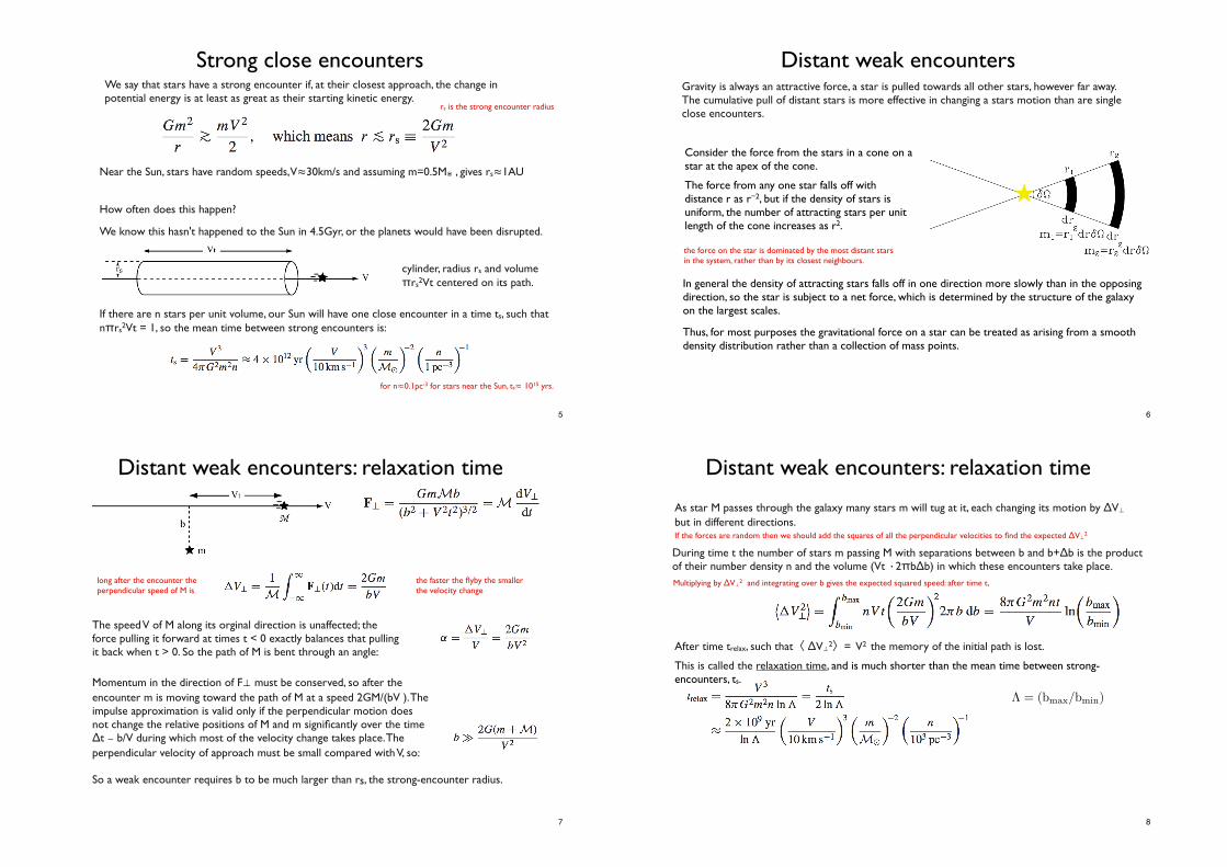
Strong close encountersWe say that stars have a strong encounter if, at their closest approach, the change in potential energy is at least as great as their starting kinetic energy.

rs is the strong encounter radius

Near the Sun, stars have random speeds, V≈30km/s and assuming m=0.5M⦿ , gives rs≈1AU

How often does this happen?

We know this hasn't happened to the Sun in 4.5Gyr, or the planets would have been disrupted.

cylinder, radius rs and volume πrs2Vt centered on its path.

If there are n stars per unit volume, our Sun will have one close encounter in a time ts, such that nπrs2Vt = 1, so the mean time between strong encounters is:

for n≈0.1pc-3 for stars near the Sun, ts≈ 1015 yrs.

5

Distant weak encountersGravity is always an attractive force, a star is pulled towards all other stars, however far away. The cumulative pull of distant stars is more effective in changing a stars motion than are single close encounters.

★

Consider the force from the stars in a cone on a star at the apex of the cone.

The force from any one star falls off with distance r as r−2, but if the density of stars is uniform, the number of attracting stars per unit length of the cone increases as r2.

In general the density of attracting stars falls off in one direction more slowly than in the opposing direction, so the star is subject to a net force, which is determined by the structure of the galaxy on the largest scales.

Thus, for most purposes the gravitational force on a star can be treated as arising from a smooth density distribution rather than a collection of mass points.

the force on the star is dominated by the most distant stars in the system, rather than by its closest neighbours.

6

Distant weak encounters: relaxation time

long after the encounter the perpendicular speed of M is

the faster the flyby the smaller the velocity change

The speed V of M along its orginal direction is unaffected; the force pulling it forward at times t < 0 exactly balances that pulling it back when t > 0. So the path of M is bent through an angle:

Momentum in the direction of F⊥ must be conserved, so after the encounter m is moving toward the path of M at a speed 2GM/(bV ). The impulse approximation is valid only if the perpendicular motion does not change the relative positions of M and m significantly over the time Δt ∼ b/V during which most of the velocity change takes place. The perpendicular velocity of approach must be small compared with V, so:

So a weak encounter requires b to be much larger than rs, the strong-encounter radius.

7

⇤ = (bmax

/bmin

)

Distant weak encounters: relaxation time

As star M passes through the galaxy many stars m will tug at it, each changing its motion by ΔV⊥ but in different directions.

During time t the number of stars m passing M with separations between b and b+Δb is the product of their number density n and the volume (Vt ·2πbΔb) in which these encounters take place.

After time trelax, such that〈 ΔV⊥2〉= V2 the memory of the initial path is lost.

This is called the relaxation time, and is much shorter than the mean time between strong-encounters, ts.

If the forces are random then we should add the squares of all the perpendicular velocities to find the expected ΔV⊥2

Multiplying by ΔV⊥2 and integrating over b gives the expected squared speed: after time t,

8

Distant weak encounters: relaxation time

What should be the value of Λ ?

⇤ = (bmax

/bmin

)

Although the many weak pulls of distant stars change the direction of motion of a star like the Sun more rapidly than do the very infrequent close encounters, the time required is still ∼1013 yr, which is much longer than the age of the Universe. The exact values of bmin and bmax are thus clearly not important.

For stars near the Sun, rs = 1 AU, and 300 pc ≤bmax ≤30 kpc, giving ln Λ ≈ 18–22.

The equation is certainly not valid if b < rs, and so bmin = rs and bmax is to be equal to the size of the whole stellar system.

So, when calculating the motion of stars like the Sun, we can ignore the pulls of individual stars, and consider all the stars to move in the smoothed-out potential of the entire Galaxy.

In ω Centauri, trelax ~ 5 Gyr. This is much longer than tcross ≈ 0.5 Myr, the time that a star takes to move across the core. We can safely calculate the path of a star over a few orbits by using only the smoothed part of the gravitational force. To understand how globular clusters change throughout the lifetime of the Galaxy, we must take account of energy exchanges between individual stars. The central parts of most clusters have been affected by relaxation.

In a galaxy with ∼1011 stars, relaxation will be important only after ~109 crossing times, which is much longer than the age of the Universe.

9

The Virial TheoremA key concept in astronomy, from stars to star clusters to galaxies to galaxy clusters to the formation of galaxies, is the concept of virialization

Gravitationally-bound systems in equilibrium obey the remarkable property that their total energy is always one-half of their (time-averaged) potential energy

2hT i+ hUi = 0

Where T is the total kinetic energy and U the total potential energy of the system.

This can be derived from the equations of motion for a system in which physical collisions are rare. For a system of N point sized bodies each with a mass mi and position xi and velocity vi :

dxi

dt= vi

dvi

dt=

X

j 6=i

Gmj(rj � ri)

|rj � ri|3

N-body systems obey several basic conservation laws

10

The Virial Theorem

The virial theorem is the primary tool for finding the mass of star clusters and galaxies where the orbits are far from circular. Unless a system is actively colliding with another, or is still forming by collapse, we assume it is close to a steady state, so that the virial theorem applies.

11

The Virial Theorem

Stars in an isolated cluster can change their kinetic and potential energies, as long as the sum of these remains constant.

the total energy of a cluster of stars (PE+KE) is constant.

The virial theorem tells us how, on average, the kinetic and potential energies are in balance.

But star clusters cannot remain in this state, as the member stars are continuously accelerated into motion.

If the stars moved so far apart that their speeds dropped to zero, and then just stayed there, the system could still satisfy this equation.

As they move further apart, their potential energy increases, and their speeds must drop so that the kinetic energy can decrease.

KE = �1

2PE

The virial theorem states that, for a stable, self-gravitating, spherical distribution of equal mass objects (stars, galaxies, etc), the total potential energy must equal the total kinetic energy, within a factor of two.

12

The Virial Theorem

For a nearly spherical, non-rotating system, we assume the M/L is constant within the system, so that the measured surface brightness indicates the mass density.

Measure the stellar radial velocities Vr with respect to the mean motion of the system, and so find the velocity dispersion σr. This is defined σr2 = 〈Vr2〉averaged over the system.

Many systems are too distant to be able to measure the tangential motions, so it is assumed that the motions are isotropic, then 〈vα ·vα〉≈ 3σr2, and the KE ≈ (3σr2/2) (M/L) Ltot.

From the surface brightness we can find the volume density of stars and hence the PE.

To find the average motion of one star within an unchanging potential, we can regard the gravity of all other stars as giving rise to an external force. For each star the virial theorem tells us

v2 ⇡ GM

R

13

Orbits of stars in spherical systems

14

Orbits of stars in spherical systems

Let's examine the orbits of individual stars in gravitational fields such as those found in stellar systems and consider what kinds of orbits are possible in a spherically symmetric, or an axially symmetric potential

15

Orbits of stars in spherical systemsWhen finding the orbit of a single star moving through a galaxy, we can usually ignore the effect which that star has in attracting all the other stars, and thus changing the gravitational potential

E � 12mv2 + m�(x) = constant

If the mass distribution is static (not changing), the potential at position x does not change with time.

Taking the scalar product of v withd

dt(mv) = �m��(x) with �(x) = �

�

�

Gm�

|x� x�| for x �= x�

The star's energy ε is the sum of the KE =mv2/2 and the PE = m Φ(x).

16

Orbits of disc starsSince we are dealing only with gravitational forces, the trajectory of a star in a given field does not depend on its mass.

Eqn. of motion of a star

the cross product of any vector with itself is zero

This finding greatly simplifies the determination of the star’s orbit, for now that we have established that the star moves in a plane, we may simply use plane polar coordinates (r,ψ) in which the center of attraction is at r = 0 and ψ is the azimuthal angle in the orbital plane.

L is simply the angular momentum per unit mass, a vector perpendicular to the plane defined by the star’s instantaneous position and velocity vectors.

Since this vector is constant, we conclude that the star moves in a plane, the orbital plane.

17

Orbits of disc starsFor the disc, the motion of a star is restricted to an orbital plane, and only two coordinates are needed to describe the location of the star. Eqn. of motion in cylinderical coords make sense.

φ

Galacto-centric cylinderical polar coords (R, φ, z). z=0

R=0

R = R'2 � @�

@R

= �@�eff

@R�eff ⌘ �(R, z) +

L2z

2R2The effective potential Φeff(R, z; Lz) behaves like a potential energy for the star’s motion in R and z.

d

dt(R2') = Lz = 2RR'+R2'

= R(2R'+R') = 0 no force in φ; mv conserved

R = r�

The Eqns of motion (R, φ, z):

R�R'2 = �@�

@R2R'+R' = 0

z = �@�

@z

minimum - circular motion

18

Plummer profile

Since Ṙ2 ≥ 0, the Lz2 term in Φeff acts as an "angular-momentum barrier", preventing a star with Lz≠0 from coming closer to R=0 than Ṙ=0.

Each star must remain within an apogalactic outer limit.

A star with angular momentum Lz can follow an exactly circular orbit with Ṙ=0 only at radius Rg where the effective potential Φeff is stationary with respect to R.

Ω(Rg) is the angular speed of the circular orbit in the plane z=0

a circular orbit has the least energy for a given Lz. The orbit is stable. Any star with same Lz must oscillate around it.

follows an elliptical epicycle around the guiding centre, which moves with angular speed Ω(Rg) in a circular orbit with radius Rg.

Orbits of stars in an axisymmetric galaxy

19

All of these equations can actually be derived from the “collisionless Boltzmann equation” (or the Liouville equation), which describes the paths of stars in phase space

We can describe the stars in a galaxy as we usually describe atoms in a gas or a fluid: not by following the path of each atom, but by asking about the density of atoms in a particular region and about their average motion. For simplicity, we need to assume that all the stars have the same mass m.

Let’s assume we have a large number of stars moving in a smooth potential

The distribution function f (x, v, t ) gives the probability density in the six-dimensional phase space of (x, v). The average number of particles (stars or atoms) in a cube of sides Δx,Δy, and Δz centred at x, that have x velocity between vx and vx + Δvx , y velocity between vy and vy + Δvy , and z velocity between vz and vz +Δvz

The Collisionless Boltzmann Equation (CBE)

We want to find equations to relate changes in the density and the distribution function, as stars move about in the Galaxy, to the gravitational potential Φ(x, t ).

20

Since the potential is smooth, neighboring particles in phase space (at the same x,v) move together, and we can use the fluid approximation:

Finally, the flow is smooth: stars do not jump discontinuously from one region of phase space to another — no collisions

Then f (density in phase space)has to satisfy a continuity equation:

w = (x,v)w = (v,���)

phase space divergence

(5)�f

�t+�6 · (fw) = 0

The conservation of fluid mass is described by the continuity equation

increase in number of stars over the volume

flow integral OUT of volumedensity only increases if stars flow in.

21

Expand equation (5):

Consider the term . This is the divergence of the flow in phase space. Let’s now show that this is incompressible:

Flow in phase space is incompressible as long as the forces do not depend on particle velocity

�f

�t+ f�6 · (w) + w ·�6f = 0

�6 · (w)

�6 · (w) =6�

i=1

�wi

�wi=

3�

i=1

��vi

�xi+

�vi

�vi

�= 0

vi and xi are independent assumed a potential, so�vi/�vi = 0=0 no dependence

on v

22

The result is the CBE for incompressible flow in phase space:

or

This means that the Lagrangian derivative, the change in the local density of phase-space particles seen by an observer moving with the phase-space fluid at a velocity , is zero:

�f

�t+ w ·�6f = 0

�f

�t+ v ·⇥f �⇥� · �f

�v= 0 (6)

w Df

Dt=

�f

�t+

6�

i=1

wi�f

�wi= 0

The collisionless Boltzmann equation is like the equation of continuity, but it allows for changes in velocity and relates the changes in f (x, v, t ) to the forces acting on individual stars.

two-body encounters are unimportant, so that the acceleration dv/dt of an individual star depends only on the smoothed potential Φ(x, t ).

Collisionless Boltzmann Equation

can calculate evolution of any f with time

23

This Liouville’s theorem: phase-space densities along particle trajectories are constant

Two key assumptions:

No small scale structure in the potential inside a volume element and no discontinuous jumps out of the volume element, so stars in the element are conserved: collisionless system

No frictional drag or encounters where energy and/or momentum can be exchanged with other stars: no entropy increase

or mass-density is conserved, which means the flow in phase space is incompressible, as the density is constant along a flow line.

if region gets more dense vel. disp increases, and less dense decreases

24

We are going to “take moments” of the CBE by multiplying f by powers of v project out velocity dimensions

First, let’s define the space density (of the stellar population component we’re interested in) as

This is the zeroth moment in the velocity of the distribution function

Moments of the CBE: the Jeans Equations

� ��

f d3v

Often, we do not solve the collisionless Boltzmann equation, which is a partial differential equation obeyed by a 6D function, explicitly but rather integrate to take velocity-moments.

25

The first and second moments in velocity of f are

Now, the zeroth moment (in velocity) of the CBE is

note that here the summation convention, where repeated indices are summed over

�vi� =1�

�vif d3v

�vivj� =1�

�vivjf d3v

��f

�td3v +

�vi

�f

�xid3v � ��

�xi

��f

�vid3v = 0

Take the CBE and integrate in all v

26

This can be rewritten as

But the last term is 0, because

And so

or

which is the continuity equation in x space (conservation of mass)

�

�t

�f d3v +

�

�xi

�vif d3v � ��

�xi

� �dv1dv2

� v3=+�

v3=���f = 0

f(vi)|+��� = 0 if limvi��

f = 0

⇥�

⇥t+

⇥

⇥xi(�vi) = 0

⇥�

⇥t+� · (�v) = 0 (7)FIRST JEANS EQN

simplified 6D phase space under the assumption that the medium is incompresible

27

The first moment in velocity of the CBE is

Now,

so

�vj

�f

�td3v +

�vivj

�f

�xid3v � ��

�xi

�vj

�f

�vid3v = 0

�vj

⇤f

⇤vid3v =

� �dv1dv2

� v3=+�

v3=��⇤f �

� �⇤vj

⇤vi

�f d3v

= 0� �ij⇥⇥

⇥t(��vj�) +

⇥

⇥xi(��vivj�) + �

⇥�⇥xj

= 0

�vi� =1�

�vif d3v

�vivj� =1�

�vivjf d3v

28

Subtracting off the zeroth moment, we have

We usually rewrite this in terms of the velocity dispersion tensor, the velocity dispersion about the mean (streaming) motion:

�⇥�vj�⇥t

� �vi�⇥

⇥xi(��vj�) +

⇥

⇥xi(��vivj�) + �

⇥�⇥xj

= 0

�2ij = �(vi � �vi�)(vj � �vj�)� = �vivj� � �vi��vj�

29

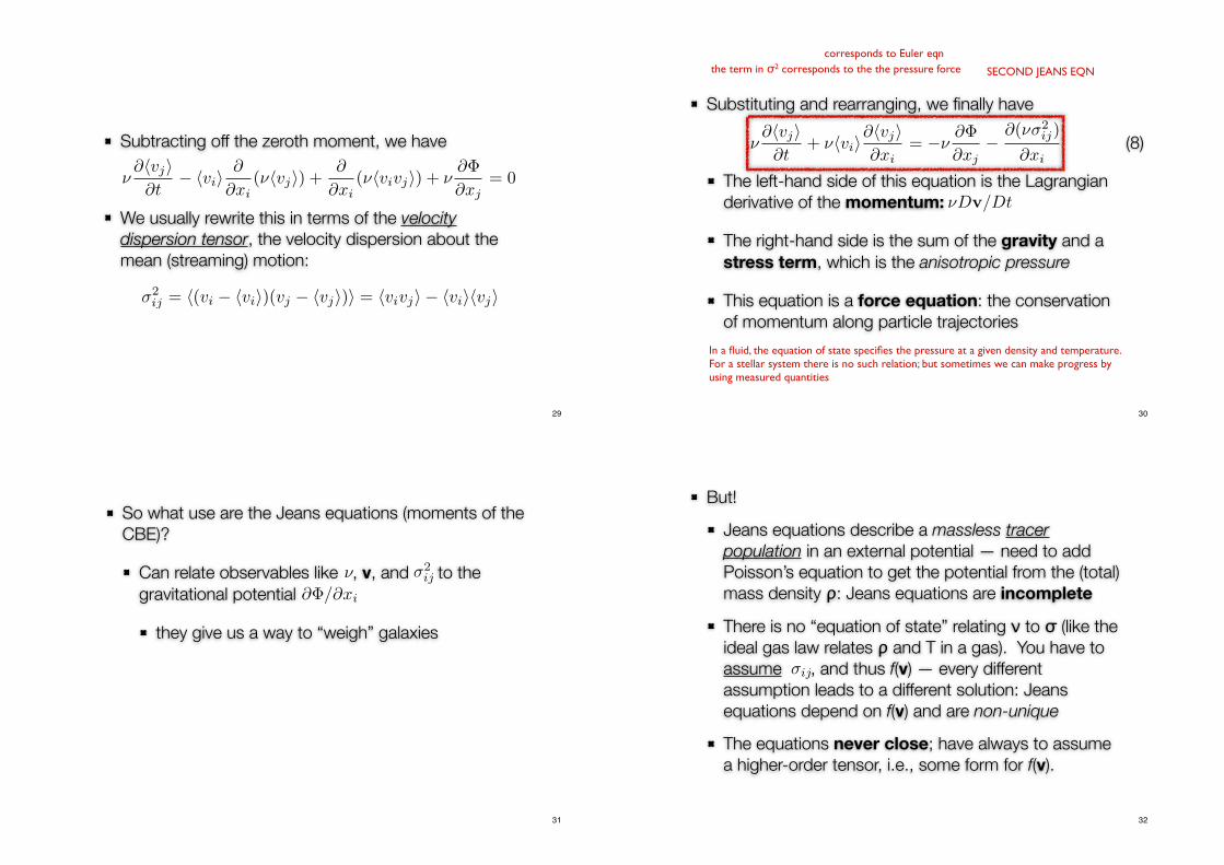
Substituting and rearranging, we finally have

The left-hand side of this equation is the Lagrangian derivative of the momentum:

The right-hand side is the sum of the gravity and a stress term, which is the anisotropic pressure

This equation is a force equation: the conservation of momentum along particle trajectories

�⇤�vj�⇤t

+ ��vi�⇤�vj�⇤xi

= ��⇤�⇤xj

�⇤(�⇥2

ij)⇤xi

(8)

�Dv/Dt

SECOND JEANS EQN

corresponds to Euler eqn the term in σ2 corresponds to the the pressure force

In a fluid, the equation of state specifies the pressure at a given density and temperature. For a stellar system there is no such relation; but sometimes we can make progress by using measured quantities

30

Since the velocity dispersion tensor is symmetric, it can be diagonalized. This diagonalized tensor is the velocity ellipsoid, which we met earlier...

So what use are the Jeans equations (moments of the CBE)?

Can relate observables like , v, and to the gravitational potential

they give us a way to “weigh” galaxies

�2ij�

��/�xi

31

But!

Jeans equations describe a massless tracer population in an external potential — need to add Poisson’s equation to get the potential from the (total) mass density ρ: Jeans equations are incomplete

There is no “equation of state” relating ν to σ (like the ideal gas law relates ρ and T in a gas). You have to assume , and thus f(v) — every different assumption leads to a different solution: Jeans equations depend on f(v) and are non-unique

The equations never close; have always to assume a higher-order tensor, i.e., some form for f(v).

�ij

32

Let’s evaluate the quantity

the amount a population lags behind the circular velocity

Write second moment of the Jeans equation in cylindrical coordinates to find:

In the Solar Neighborhood, the term in brackets is ~4

Asymmetric drift: an application of the Jeans eqn

va � vc � �v��

2vcva ⇥ ⇤v2R⌅

�⇥2

⇤v2R⌅

� 32� 2

⇤ ln �

⇤ lnR+

12⇤v2

z⌅⇤v2

R⌅±

�⇤v2

z⌅⇤v2

R⌅� 1

��

33

So the lag is

In the absence of radial streaming,

As increases, the population lags more behind the circular motion — hot populations rotate slower

Energy comes out of ordered motion and is put into disordered motion

�v2R� = �2

R

va � 4�v2R�/440 km s�1 � �v2

R�/110 km s�1

�2R

34

This is why depends on the velocity dispersion of the population used to measure it — older populations have higher velocity dispersions and rotate slower

V�

Stromberg’s asymmetric drift equation [e.g. equation (4-34) of

Binney & Tremaine (1987, hereafter BT)]. That is, V increases

systematically with S2 because the larger a stellar group’s velocity

dispersion is, the more slowly it rotates about the Galactic Centre

and the faster the Sun moves with respect to its lagging frame.

For very early-type stars with B ¹ V ! 0:1 mag and/or S!

15 km s¹1, the V-component of vh i decreases with increasing S,

colour, and hence age contradicting the explanation given in the last

paragraphs. However, the stars concerned are very young, and there

are several possibilities for them not to follow the general trend.

First, because of their youth these stars are unlikely to constitute a

kinematically well-mixed sample; rather, they move close to the

orbit of their parent cloud; many will belong to a handful of moving

groups. Secondly, Stromberg’s asymmetric drift relation predicts a

linear relation between V and S2 only if both the shape of the

velocity ellipsoid, i.e. the ratios of the eigenvalues of j, and the

radial density gradient are independent of S. Young stars probably

violate these assumptions, especially the latter one.

The radial and vertical components U0 and W0 of the velocity of

the Sun with respect to the LSR (the velocity of the closed orbit in

the plane that passes through the location of the Sun) can be derived

from hvi estimated for all stars together. The component in the

direction of rotation, V0, may be read off from Fig. 4 by linearly

extrapolating back to S ¼ 0. Ignoring stars blueward of

B ¹ V ¼ 0 mag we find

U0 ¼ 10:00 " 0:36 ð"0:08Þ km s¹1;

V0 ¼ 5:25 " 0:62 ð"0:03Þ km s¹1;

W0 ¼ 7:17 " 0:38 ð"0:09Þ km s¹1;

ð20Þ

where the possible effect arising from a systematic error of 0:1 mas

in the parallax is given in brackets. When we use this value of the

Local stellar kinematics 391

! 1998 RAS, MNRAS 298, 387–394

Figure 3. The components U, V and W of the solar motion with respect to stars with different colour B ¹ V. Also shown is the variation of the dispersion S with

colour.

Figure 4. The dependence of U, V and W on S2. The dotted lines correspond to the linear relation fitted (V) or the mean values (U and W) for stars bluer than

B ¹ V ¼ 0:

35

Weighing the MW disk

Let’s use the Jeans eqns to see if we can measure the mass of the MW disk in the Solar Neighborhood

First, select a tracer population like K dwarfs

Now assume that the potential is constant with time

Then ν and f are also constant

High above the plane,

Then from the first Jeans eqn, Eq. (7), everywhere

�vz��(z) � 0

�vz� = 0

36

Now we can use the second Jeans eqn, Eq. (8):

Next we need Poisson’s equation in cylindrical coordinates:

Then we can write

4�G⇥(R, z) =⇤2�⇤z2

+1R

⇤

⇤R

�R

⇤�⇤R

�

���R

=v2

c (R)R

d

dz[�(z)⇥2

z ] = �⇤�⇤z

�(z)

37

and so we have

Near the Sun, the rotation curve is nearly flat, so the last term can be ignored

To find ρ we need to differentiate ν twice, which is very sensitive to small errors! Let’s concentrate on the surface density instead:

4⇥G⇤(R, z) =d

dz

�� 1

�(z)d

dz[�(z)⌅2

z ]�

+1R

⇧v2c (R)⇧R

2⇥G�(< z) = 2⇥G

� +z

�z⇤(z�)dz� � � 1

�(z)d

dz[�(z)⌅2

z ]

38

Oort was the first to try this (and derive the equations), using K giants and F dwarfs

He assumed σz did not vary with distance from the plane and found

But at z>1 kpc, Σ(z) began to decrease!

σz is not constant with distance from the plane...

Using K dwarfs and allowing σz to vary, Kuijken & Gilmore (1991) found

�(< 700 pc) � 90 M� pc�2

�(< 1100 pc) = 71± 6 M� pc�2

39

The total surface density in gas and stars in this range is ~40–55 M⊙ pc–2

But not all of the surface density determined by K&G is actually in the disk (some must be in the halo), so the amount of dark matter in the disk is probably negligible

40