lecture: network flow problems and combinatorial
TRANSCRIPT

Lecture: Network Flow Problems andCombinatorial Optimization Problems
http://bicmr.pku.edu.cn/~wenzw/bigdata2016.html
Acknowledgement: this slides is based on Prof. James B. Orlin’s lecture notes of“15.082/6.855J, Introduction to Network Optimization” at MIT, as well as Prof. Shaddin
Dughmi and Prof. Sewoong Oh’s lecture notes
Textbook: Network Flows: Theory, Algorithms, and Applications by Ahuja, Magnanti, andOrlin referred to as AMO
1/66

2/66
Outline
1 Introduction to Maximum Flows
2 The Ford-Fulkerson Maximum Flow Algorithm
3 Maximum Bipartite Matching
4 The Minimum Cost Spanning Tree Problem

3/66
Maximum Flows
We refer to a flow x as maximum if it is feasible and maximizes v. Ourobjective in the max flow problem is to find a maximum flow.
A max flow problem. Capacities and a non- optimum flow.
4/66
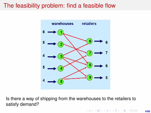
The feasibility problem: find a feasible flow
Is there a way of shipping from the warehouses to the retailers tosatisfy demand?
5/66
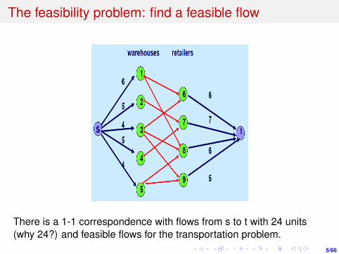
The feasibility problem: find a feasible flow
There is a 1-1 correspondence with flows from s to t with 24 units(why 24?) and feasible flows for the transportation problem.
6/66
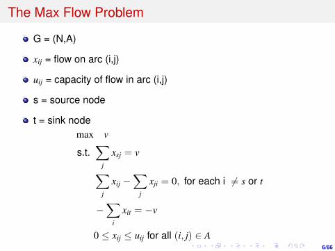
The Max Flow Problem
G = (N,A)
xij = flow on arc (i,j)
uij = capacity of flow in arc (i,j)
s = source node
t = sink nodemax v
s.t.∑
j
xsj = v
∑j
xij −∑
j
xji = 0, for each i 6= s or t
−∑
i
xit = −v
0 ≤ xij ≤ uij for all (i, j) ∈ A

7/66
Dual of the Max Flow Problem
reformulation:Ai,(i,j) = 1,Aj,(i,j) = −1, for (i, j) ∈ A and all other elements are 0A>y = yi − yj
The primal-dual pair is
min (0,−1)(x, v)>
s.t. Ax + (−1, 0, 1)>v = 0
Ix + 0>v ≤ u
x ≥ 0, v is free
⇐⇒
max − u>π
s.t. A>y + I>π ≥ 0
− 1 + (−1, 0, 1)y = 0
π ≥ 0
Hence, we have the dual problem:
min u>π
s.t. yj − yi ≤ πij, ∀(i, j) ∈ A
yt − ys = 1
π ≥ 0

8/66
Duality of the Max Flow Problem
The primal-dual of the max flow problem is
max v
s.t.∑
j
xsj = v
∑j
xij −∑
j
xji = 0,∀i /∈ {s, t}
−∑
i
xit = −v
0 ≤ xij ≤ uij ∀(i, j) ∈ A
min u>π
s.t. yj − yi ≤ πij, ∀(i, j) ∈ A
yt − ys = 1
π ≥ 0

9/66
Duality of the Max Flow Problem
Dual solution describes fraction πij of each edge to fractionallycut
Dual constraints require that at least 1 edge is cut on every pathP from s to t. ∑
(i,j)∈P
πij ≥∑
(i,j)∈P
yj − yi = yt − ys = 1
Every integral s-t cut (A,B) is feasible:πij = 1, ∀i ∈ A, j ∈ B, otherwise, πij = 0.yi = 0 if i ∈ A and yj = 1 if i ∈ B
weak duality: v ≤ u>π for any feasible solutionmax flow ≤ minimum flow
strong duality: v∗ = u>π∗ at the optimal solution

10/66
Outline
1 Introduction to Maximum Flows
2 The Ford-Fulkerson Maximum Flow Algorithm
3 Maximum Bipartite Matching
4 The Minimum Cost Spanning Tree Problem

11/66
sending flows along s-t paths
One can find a larger flow from s to t by sending 1 unit of flow alongthe path s-2-t

12/66
A different kind of path
One could also find a larger flow from s to t by sending 1 unit of flowalong the path s-2-1-t. (Backward arcs have their flow decreased.)
Decreasing flow in (1, 2) is mathematically equivalent to sending flowin (2, 1) w.r.t. node balance constraints.

13/66
The Residual Network
The Residual Network G(x)We let rij denote theresidual capacity of arc (i,j)

14/66
A Useful Idea: Augmenting Paths
An augmenting path is a path from s to t in the residual network.
The residual capacity of the augmenting path P isδ(P) = min{rij : (i, j) ∈ P}.
To augment along P is to send δ(P) units of flow along each arcof the path. We modify x and the residual capacitiesappropriately.
rij := rij − δ(P) and rji := rji + δ(P) for (i,j) ∈P.
15/66
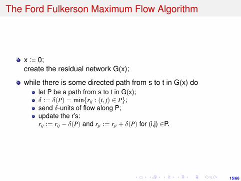
The Ford Fulkerson Maximum Flow Algorithm
x := 0;create the residual network G(x);
while there is some directed path from s to t in G(x) dolet P be a path from s to t in G(x);δ := δ(P) = min{rij : (i, j) ∈ P};send δ-units of flow along P;update the r’s:rij := rij − δ(P) and rji := rji + δ(P) for (i,j) ∈P.

16/66
To prove correctness of the algorithm
Invariant: at each iteration, there is a feasible flow from s to t.
Finiteness (assuming capacities are integral and finite):The residual capacities are always integer valuedThe residual capacities out of node s decrease by at least oneafter each update.
CorrectnessIf there is no augmenting path, then the flow must be maximum.max-flow min-cut theorem.

17/66
Integrality
Assume that all data are integral.
Lemma: At each iteration all residual capacities are integral.Proof. It is true at the beginning. Assume it is true after the firstk-1 augmentations, and consider augmentation k along path P.
The residual capacity δ of P is the smallest residual capacity onP, which is integral.
After updating, we modify residual capacities by 0, or δ, and thusresidual capacities stay integral.

18/66
Theorem. The Ford-Fulkerson Algorithm is finite
Proof. The capacity of each augmenting path is at least 1.
rsj decreases for some j.
So, the sum of the residual capacities of arcs out of s decreasesat least 1 per iteration.
Number of augmentations is O(nU), where U is the largestcapacity in the network.

19/66
To be proved: If there is no augmenting path, then the flow ismaximum
G(x) = residual network forflow x.x* = final flowIf there is a directed path fromi to j in G, we write i→ j.
S* = { j : s→ j in G(x*)}T*=N\S*

20/66
Lemma: there is no arc in G(x*) from S* to T*
S* = { j : s→ j in G(x*)}T*=N\S*
Proof: If there were such an arc(i, j) and i ∈ S∗, then j would be inS*.
21/66
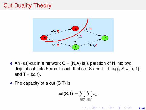
Cut Duality Theory
An (s,t)-cut in a network G = (N,A) is a partition of N into twodisjoint subsets S and T such that s ∈ S and t ∈T, e.g., S = {s, 1}and T = {2, t}.
The capacity of a cut (S,T) is
cut(S,T) =∑i∈S
∑j∈T
uij
22/66
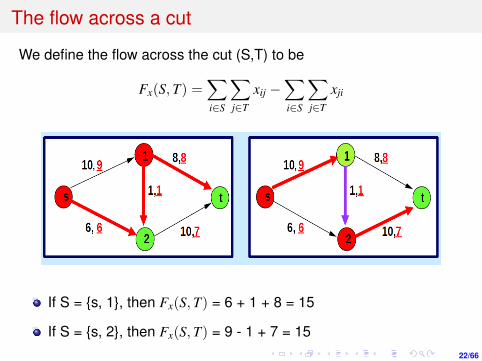
The flow across a cut
We define the flow across the cut (S,T) to be
Fx(S,T) =∑i∈S
∑j∈T
xij −∑i∈S
∑j∈T
xji
If S = {s, 1}, then Fx(S,T) = 6 + 1 + 8 = 15
If S = {s, 2}, then Fx(S,T) = 9 - 1 + 7 = 15

23/66
Max Flow Min Cut
Theorem. (Max-flow Min-Cut). The maximum flow value is theminimum value of a cut.
Proof. The proof will rely on the following three lemmas:
Lemma 1. For any flow x, and for any s-t cut (S, T), the flow outof s equals Fx(S,T).
Lemma 2. For any flow x, and for any s-t cut (S, T),Fx(S,T) ≤ cut(S,T).
Lemma 3. Suppose that x* is a feasible s-t flow with noaugmenting path. Let S* = {j : s→j in G(x*)} and let T* = N\S.Then Fx∗(S∗,T∗) = cut(S∗,T∗).

24/66
Proof of Theorem (using the 3 lemmas)
Let x’ be a maximum flowLet v’ be the maximum flow valueLet x* be the final flow.Let v* be the flow out of node s (for x*)Let S* be nodes reachable in G(x*) from s.Let T* = N\S*.
1 v* ≤ v’, by definition of v’2 v’ = Fx′ (S*, T*), by Lemma 1.3 Fx′ (S*, T*) ≤ cut(S*, T*) by Lemma 2.4 v* = Fx∗ (S*, T*) = cut(S*, T*) by Lemmas 1,3.
Thus all inequalities are equalities and v* = v’.

25/66
Proof of Lemma 1
Proof. Add the conservation of flow constraints for each node i∈S -{s} to the constraint that the flow leaving s is v. The resulting equalityis Fx (S,T) = v.
xs1 + xs2 = v, x12 + x1t − xs1 = 0 =⇒ xs2 + x12 + x1t = v
xs1 + xs2 = v, x2t − xs2 − x12 = 0 =⇒ xs1 − x12 + x2t = v

26/66
Proof of Lemma 2
Proof. If i ∈S, and j ∈T, then xij ≤ uij. If i ∈T, and j ∈S, then xij ≥ 0.
Fx(S,T) =∑i∈S
∑j∈T
xij −∑i∈S
∑j∈T
xji
cut(S,T) =∑i∈S
∑j∈T
uij −∑i∈S
∑j∈T
0
left: Fx(S,T)=15, cut(S, T) = 15
right: Fx(S,T)=15, cut(S, T) = 20

27/66
Proof of Lemma 3.
We have already seen that there is no arc from S* to T* in G(x*).
i ∈ S∗ and j ∈ T∗ =⇒ x∗ij = uij and x∗ji = 0
Otherwise, there is an arc (i, j) in G(x*)
Therefore Fx∗ (S*, T*) = cut(S*, T*)

28/66
Review
Corollary. If the capacities are finite integers, then theFord-Fulkerson Augmenting Path Algorithm terminates in finitetime with a maximum flow from s to t.
Corollary. If the capacities are finite rational numbers, then theFord-Fulkerson Augmenting Path Algorithm terminates in finitetime with a maximum flow from s to t. (why?)
Corollary. To obtain a minimum cut from a maximum flow x*, letS* denote all nodes reachable from s in G(x*), and T* = N\S*
Remark. This does not establish finiteness if uij =∞ or ifcapacities may be irrational.

29/66
Speedups of the augmenting path algorithm
Shortest augmenting path algorithm: always augment along thepath in G(x) with the fewest number of arcs.
Largest augmenting path algorithm: always augment along apath in G(x) with the greatest capacity.

30/66
The shortest augmenting path algorithm
x := 0;create the residual network G(x);
while there is some directed path from s to t in G(x) dolet P be a path from s to t in G(x) with the fewest number of arcs;δ := δ(P) = min{rij : (i, j) ∈ P};send δ-units of flow along P;update the r’s:rij := rij − δ(P) and rji := rji + δ(P) for (i,j) ∈P.
Theorem. The shortest augmenting path algorithm determines amaximum flow in O(nm) augmentations.
This algorithm can be implemented to run in O(n2m) time.

31/66
Distance Labels
Let d(i) be the length of the shortest path from i to t in G(x)
FACT 1: If (i, j)∈G(x), then d(i) ≤ d(j) + 1.
FACT 2: Arc (i, j) is on a shortest path from i to t if and only if d(i)= d(j) + 1.
FACT 3: d(t) = 0; d(i) < n for all i s.t. i→ t in G(x).

32/66
Valid Arcs and Saturating Pushes
An arc (i, j) ∈ G(x) isvalid if d(i) = d(j) + 1.FACT: If P is anaugmenting path, thenevery arc of P is valid.
Suppose δ units of flow are sent along P. The augmentation saturatesarc (i, j) ∈ P if rij = δ.

33/66
The number of augmenting paths
Theorem. The number of augmenting paths for the shortestaugmenting path algorithm is O(nm).
Fact. In every augmenting path, at least one arc (i, j) is saturated.
Lemma 1. Arc (i, j) and its reversal (j, i) can be saturated at most n/2times each. (To be proved later.)
Proof of theorem. Let aij be the number of times that arc (i, j) issaturated. Let k be the number of augmentations.
Then k ≤∑
(i,j)∈A 2aij ≤∑
(i,j)∈A n ≤ nm.

34/66
Proof of Lemma 1.
Each arc (i, j) is saturated fewer than n/2 times.Lemma 2. Let d be the distance labels at an iteration where arc(i, j) is saturated. Suppose that d’ is the vector of distance labelsat a subsequent iteration where (i, j) is saturated. Then n > d’(i)≥ d(i) + 2. (to be proved on next slide).
Proof of Lemma 1 from Lemma 2. Before (i, j) can be saturatedagain, its distance label will increase by at least 2. Since 0 < d(i)< n, the distance label can increase at most n/2 times.

35/66
Proof of Lemma 2.
Lemma 3. Let d be the distance labels at some iteration, and letd’ be the distance labels at a subsequent iteration. Then d’(i) ≥d(i) for all i∈ N. (to be proved on next slide)
Proof of Lemma 2 from Lemma 3. Suppose that (i, j) is saturatedwhen d(i) = k. There is no more flow in (i, j) until flow is sent in (j,i) at which point the distance label of j is k+1. But flow cannot bereturned in (i, j) until it is valid again, and the distance label is atleast k+2.

36/66
Proof of Lemma 3
Assume that Lemma 3 is false. Let d be the distance labels at someiteration. Let P be the augmenting path. After the augmentation, thereversals of arcs in P are in the residual network. But adding thesearcs to G(x) does not decrease any distance. And deleting arcs of Pcannot decrease a distance label.

37/66
Outline
1 Introduction to Maximum Flows
2 The Ford-Fulkerson Maximum Flow Algorithm
3 Maximum Bipartite Matching
4 The Minimum Cost Spanning Tree Problem

38/66
Matchings
An undirected network G = (N, A) isbipartite if N can be partitioned intoN1 and N2 so that for every arc (i,j), i∈ N1 and j ∈ N2.
A matching in N is a set of arcs notwo of which are incident to acommon node.
Matching Problem: Find a matchingof maximum cardinality
39/66
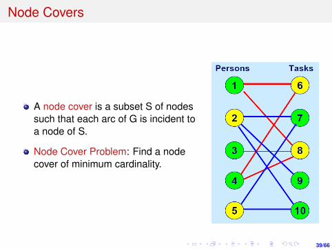
Node Covers
A node cover is a subset S of nodessuch that each arc of G is incident toa node of S.
Node Cover Problem: Find a nodecover of minimum cardinality.

40/66
Matching Duality Theorem
Theorem. König- Egerváry. Themaximum cardinality of a matching isequal to the minimum cardinality of anode cover.
Note. Every node cover has at leastas many nodes as any matchingbecause each matched edge isincident to a different node of thenode cover.

41/66
How to find a minimum node cover

42/66
Matching-Max Flow
Solving the Matching Problem as a Max Flow Problem
Replace original arcs by directed arcs with infinite capacity.
Each arc (s, i) has a capacity of 1.
Each arc (j, t) has a capacity of 1.
43/66
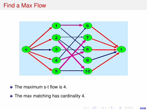
Find a Max Flow
The maximum s-t flow is 4.
The max matching has cardinality 4.

44/66
Determine the minimum cut
plot the residual network G(x)
Let S = {j : s→j in G(x)} and let T = N\S.
S = {s, 1, 3, 4, 6, 8}. T = {2, 5, 7, 9, 10, t}.
There is no arc from {1, 3, 4} to {7, 9, 10} or from {6, 8} to {2, 5}.Any such arc would have an infinite capacity.

45/66
Find the min node cover
The minimum node cover is the set of nodes incident to the arcsacross the cut. Max-Flow Min-Cut implies the duality theorem formatching.minimum node cover: {2,5,6,8}

46/66
Philip Hall’s Theorem
A perfect matching is a matching which matches all nodes of thegraph. That is, every node of the graph is incident to exactly oneedge of the matching.Philip Hall’s Theorem. If there is no perfect matching, then thereis a set S of nodes of N1 such that |S| > |T| where T are thenodes of N2 adjacent to S.

47/66
The Max-Weight Bipartite Matching Problem
Given a bipartite graph G = (N, A), with N = L ∪ R, and weights wij onedges (i,j), find a maximum weight matching.
Matching: a set of edges covering each node at most once
Let n=|N| and m = |A|.
Equivalent to maximum weight / minimum cost perfect matching.

48/66
The Max-Weight Bipartite Matching
Integer Programming (IP) formulation
max∑
ij
wijxij
s.t.∑
j
xij ≤ 1,∀i ∈ L
∑i
xij ≤ 1,∀j ∈ R
xij ∈ {0, 1},∀(i, j) ∈ A
xij = 1 indicate that we include edge (i, j ) in the matching
IP: non-convex feasible set

49/66
The Max-Weight Bipartite Matching
Integer program (IP)
max∑
ij
wijxij
s.t.∑
j
xij ≤ 1,∀i ∈ L
∑i
xij ≤ 1,∀j ∈ R
xij ∈ {0, 1},∀(i, j) ∈ A
LP relaxation
max∑
ij
wijxij
s.t.∑
j
xij ≤ 1,∀i ∈ L
∑i
xij ≤ 1,∀j ∈ R
xij ≥ 0,∀(i, j) ∈ A
Theorem. The feasible region of the matching LP is the convexhull of indicator vectors of matchings.
This is the strongest guarantee you could hope for an LPrelaxation of a combinatorial problem
Solving LP is equivalent to solving the combinatorial problem
50/66
Primal-Dual Interpretation
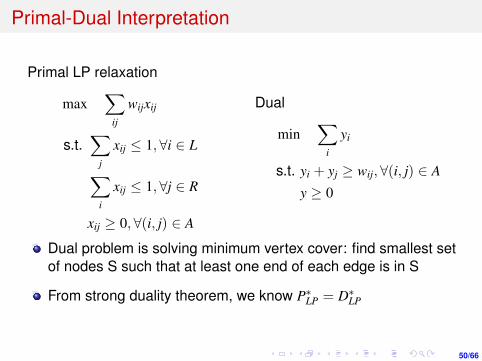
Primal LP relaxation
max∑
ij
wijxij
s.t.∑
j
xij ≤ 1,∀i ∈ L
∑i
xij ≤ 1,∀j ∈ R
xij ≥ 0,∀(i, j) ∈ A
Dual
min∑
i
yi
s.t. yi + yj ≥ wij,∀(i, j) ∈ A
y ≥ 0
Dual problem is solving minimum vertex cover: find smallest setof nodes S such that at least one end of each edge is in S
From strong duality theorem, we know P∗LP = D∗LP
51/66
Primal-Dual Interpretation
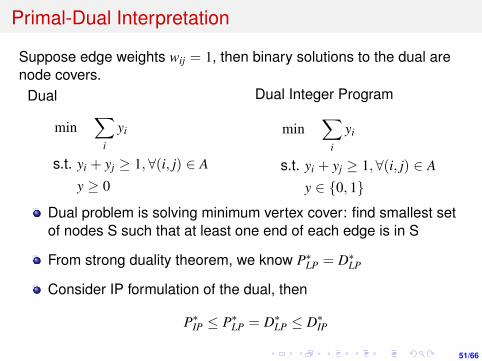
Suppose edge weights wij = 1, then binary solutions to the dual arenode covers.
Dual
min∑
i
yi
s.t. yi + yj ≥ 1, ∀(i, j) ∈ A
y ≥ 0
Dual Integer Program
min∑
i
yi
s.t. yi + yj ≥ 1, ∀(i, j) ∈ A
y ∈ {0, 1}
Dual problem is solving minimum vertex cover: find smallest setof nodes S such that at least one end of each edge is in S
From strong duality theorem, we know P∗LP = D∗LP
Consider IP formulation of the dual, then
P∗IP ≤ P∗LP = D∗LP ≤ D∗IP
52/66
Total Unimodularity
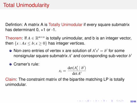
Defintion: A matrix A is Totally Unimodular if every square submatrixhas determinant 0, +1 or -1.
Theorem: If A ∈ Rm×n is totally unimodular, and b is an integer vector,then {x : Ax ≤ b; x ≥ 0} has integer vertices.
Non-zero entries of vertex x are solution of A′x′ = b′ for somenonsignular square submatrix A′ and corresponding sub-vector b′
Cramer’s rule:
xi =det(A′i | b′)
det A′
Claim: The constraint matrix of the bipartite matching LP is totallyunimodular.

53/66
The Minimum weight vertex cover
undirected graph G = (N, A) with node weights wi ≥ 0A vertex cover is a set of nodes S such that each edge has atleast one end in SThe weight of a vertex cover is sum of all weights of nodes in thecoverFind the vertex cover with minimum weight
Integer Program
min∑
i
wiyi
s.t. yi + yj ≥ 1, ∀(i, j) ∈ A
y ∈ {0, 1}
LP Relaxation
min∑
i
wiyi
s.t. yi + yj ≥ 1, ∀(i, j) ∈ A
y ≥ 0
54/66
LP Relaxation for the Minimum weight vertex cover
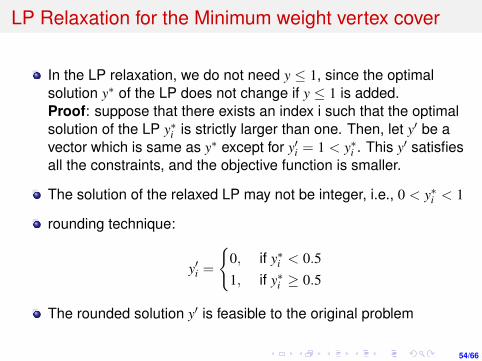
In the LP relaxation, we do not need y ≤ 1, since the optimalsolution y∗ of the LP does not change if y ≤ 1 is added.Proof: suppose that there exists an index i such that the optimalsolution of the LP y∗i is strictly larger than one. Then, let y′ be avector which is same as y∗ except for y′i = 1 < y∗i . This y′ satisfiesall the constraints, and the objective function is smaller.
The solution of the relaxed LP may not be integer, i.e., 0 < y∗i < 1
rounding technique:
y′i =
{0, if y∗i < 0.51, if y∗i ≥ 0.5
The rounded solution y′ is feasible to the original problem

55/66
LP Relaxation for the Minimum weight vertex cover
The weight of the vertex cover we get from rounding is at most twiceas large as the minimum weight vertex cover.
Note that y′i = min(b2y∗i c, 1)
Let P∗IP be the optimal solution for IP, and P∗LP be the optimalsolution for the LP relaxation
Since any feasible solution for IP is also feasible in LP, P∗LP ≤ P∗IP
The rounded solution y′ satisfy∑i
y′iwi =∑
i
min(b2y∗i c, 1)wi ≤∑
i
2y∗i wi = 2P∗LP ≤ 2P∗IP

56/66
Outline
1 Introduction to Maximum Flows
2 The Ford-Fulkerson Maximum Flow Algorithm
3 Maximum Bipartite Matching
4 The Minimum Cost Spanning Tree Problem

57/66
The Minimum Cost Spanning Tree (MST) Problem
Given a connected undirected graph G = (N, A), and costs wij onedges (i, j), find a minimum cost spanning tree of G.
Spanning Tree: an acyclic set of edges connecting every pair ofnodes
When graph is disconnected, can search for min-cost spanningforest instead
We use n and m to denote |N| and |A|, respectively.
58/66
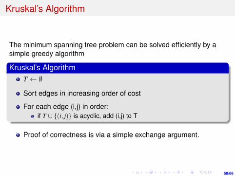
Kruskal’s Algorithm
The minimum spanning tree problem can be solved efficiently by asimple greedy algorithm
Kruskal’s AlgorithmT ← ∅
Sort edges in increasing order of cost
For each edge (i,j) in order:if T ∪ {(i, j)} is acyclic, add (i,j) to T
Proof of correctness is via a simple exchange argument.

59/66
MST Linear Program
Integer program (IP)
min∑
(i,j)∈A
wijxij
s.t.∑
(i,j)∈AS
xij ≤ |S| − 1, ∀S ⊆ A
xij ∈ {0, 1}, ∀(i, j) ∈ A
LP relaxation
min∑
(i,j)∈A
wijxij
s.t.∑
(i,j)∈AS
xij ≤ |S| − 1,∀S ⊆ A
xij ≥ 0,∀(i, j) ∈ A
TheoremThe feasible region of the above LP is the convex hull of spanningtrees.
Proof by finding a dual solution with cost matching the output ofKruskal’s algorithm.

60/66
Optimization over Sets
Most combinatorial optimization problems can be thought of aschoosing the best set from a family of allowable sets
Shortest pathsMax-weight matchingtravelling sales problems (TSP)
Set system: Pair (X , I) where X is a finite ground set andI ⊆ 2X are the feasible sets
Objective: often “linear”, referred to as modular
Analogues of concave convex: submodular and supermodular(in no particular order!)

61/66
Matroids
MatroidsA set system M = (X , I) is a matroid if
I ∅ ∈ II If A ∈ I and B ⊆ A, then B ∈ I (Downward Closure)I If A,B ∈ I and |B| > |A|, then ∃x ∈ B\A such that A ∪ {x} ∈ I
(Exchange Property)
Three conditions above are called the matroid axioms
A ∈ I is called an independent set of the matroid.
The union of all sets in I is called the ground set.
An independent set is called a basis if it is not a proper subset ofanother independent set.
The matroid whose independent sets are acyclic subgraphs iscalled a graphic matroid

62/66
Linear MatroidsI X is a finite set of vectors {v1, . . . , vm} ⊆ Rn
I S ∈ I iff the vectors in S are linearly independent
Downward closure: If a set of vectors is linearly independent,then every subset of it is also
Exchange property: Can always extend a low-dimensionindependent set S by adding vectors from a higher dimensionindependent set T

63/66
Uniform MatroidsI X is an arbitrary finite set {1, 2, . . . , n}I S ∈ I iff |S| ≤ k
Downward closure: If a set S has |S| ≤ k then the same holds forT ⊆ S.
Exchange property: If |S| < |T| ≤ k, then there is an element inT\S, and we can add it to S while preserving independence.

64/66
Partition MatroidsI X is the disjoint union of classes X1, . . . ,Xm
I Each class Xj has an upper bound kj
I S ∈ I iff |S ∩ Xj| ≤ kj for all j
This is the “disjoint union” of a number of uniform matroids

65/66
Matroid optimization problem
DefinitionI suppose each element of the ground set of a matroid I is given
an arbitrary non-negative weight.
I The matroid optimization problem is to compute a basis withmaximum total weight.

66/66
The Greedy Algorithm on Matroids
The Greedy AlgorithmB← ∅
Sort nonnegative elements of X in decreasing order of weight{1, . . . , n} with w1 ≥ w2 ≥ . . .wn ≥ 0
For i = 1 to n:if B ∪ {i} ∈ I, add i to B
TheoremThe greedy algorithm returns the maximum weight set for everychoice of weights if and only if the set system (X , I) is a matroid.