lecture 9: integrating learning and planning - joseph …josephmodayil.com/uclrl/dyna.pdf · from...

Lecture 9: Integrating Learning and Planning


Joseph Modayil


Outline

1 Introduction

2 Model-Based Reinforcement Learning

3 Model-Based Reinforcement Learning

4 Integrated Architectures

5 Simulation-Based Search


Introduction

Model-Based Reinforcement Learning

Last lecture: learn policy directly from experience

Previous lectures: learn value function directly from experience

This lecture:

Learn model directly from experience (or be given a model)Plan with the model to construct a value function or policyIntegrate learning and planning into a single architecture


Introduction

Model-Based and Model-Free RL

Model-Free RL

No modelLearn value function (and/or policy) from experience

Model-Based RL

Learn a model from experience OR be given a modelPlan value function (and/or policy) from model


Introduction

Filling in the middle of algorithm space


Introduction

Model-Free RL

state

reward

action

at

rt

st


Introduction

Model-Based RL

state

reward

action

at

rt

st



Model-Based RL



Learning a Model

What is a Model?

A modelM is a representation of an MDP 〈S,A,P,R〉,parametrized by η

A model M = 〈Pη,Rη〉 approximates the state transitionsPη ≈ P and rewards Rη ≈ R. e.g.

St+1 ∼ Pη(St+1 | St ,At)

Rt+1 = Rη(Rt+1 | St ,At)

This particular model imposes conditional independencebetween state transitions and rewards

P [St+1,Rt+1 | St ,At ] = P [St+1 | St ,At ]P [Rt+1 | St ,At ]

Conventionally a method is called model-based when thetransition and reward dynamics are explicitly represented (tosupport planning), and as model-free otherwise. Some newmethods lie in-between these extremes.



Learning a Model

Model Learning

Goal: estimate modelMη from experience {S1,A1,R2, ...,ST}This is a supervised learning problem

S1,A1 → R2, S2

S2,A2 → R3, S3...

ST−1,AT−1 → RT ,ST

Learn a function s, a→ r and also learn a function s, a→ s ′

Pick loss function (e.g. mean-squared error), and findparameters η that minimise empirical loss



Learning a Model

Examples of Models

Table Lookup Model

Linear Expectation Model

Linear Gaussian Model

Gaussian Process Model

Deep Belief Network Model

...



Learning a Model

Table Lookup Model

Model is an explicit MDP, P̂, R̂Count visits N(s, a) to each state action pair

P̂as,s′ =

1

N(s, a)

T∑t=1

1(St ,At , St+1 = s, a, s ′)

R̂as =

1

N(s, a)

T∑t=1

1(St ,At = s, a)Rt

Alternatively

At each time-step t, record experience tuple〈St ,At ,Rt+1,St+1〉To sample model, randomly pick tuple matching 〈s, a, ·, ·〉



Learning a Model

AB Example

Two states A,B; no discounting; 8 episodes of experience

A, 0, B, 0!B, 1!B, 1!B, 1!B, 1!B, 1!B, 1!B, 0!

We have constructed a table lookup model from the experience



Planning with a Model


Given a model Mη = 〈Pη,Rη〉Solve the MDP 〈S,A,Pη,Rη〉Using favourite planning algorithm

Value iterationPolicy iterationTree search...




Sample-Based Planning

A simple but powerful approach to planning

Use the model only to generate samples

Sample experience from model

st+1 ∼ Pη(st+1 | st , at)rt+1 = Rη(rt+1 | st , at)

Apply model-free RL to samples, e.g.:

Monte-Carlo controlSarsaQ-learning

Sample-based planning methods are often more efficient




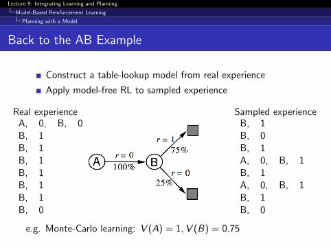
Back to the AB Example

Construct a table-lookup model from real experience

Apply model-free RL to sampled experience

Real experienceA, 0, B, 0B, 1B, 1B, 1B, 1B, 1B, 1B, 0

Sampled experienceB, 1B, 0B, 1A, 0, B, 1B, 1A, 0, B, 1B, 1B, 0

e.g. Monte-Carlo learning: V (A) = 1,V (B) = 0.75




Planning with an Inaccurate Model

Given an imperfect model 〈Pη,Rη〉 6= 〈P,R〉Performance of model-based RL is limited to optimal policyfor approximate MDP 〈S,A,Pη,Rη〉i.e. Model-based RL is only as good as the estimated model

When the model is inaccurate, planning process will computea suboptimal policy

Approach 1: when model is wrong, use model-free RL

Approach 2: reason explicitly about model uncertainty over η(e.g. Bayesian methods)

Approach 3: Combine model-based and model-free methodsin a safe way.


Integrated Architectures

Dyna

Real and Simulated Experience

We consider two sources of experience

Real experience Sampled from environment (true MDP)

s ′ ∼ Pas,s′

r = Ras

Simulated experience Sampled from model (approximate MDP)

s ′ ∼ Pη(s ′ | s, a)

r = Rη(r | s, a)



Dyna

Integrating Learning and Planning

Model-Free RL

No modelLearn value function (and/or policy) from real experience

Model-Based RL (using Sample-Based Planning)

Learn a model from real experiencePlan value function (and/or policy) from simulated experience

Dyna

Learn a model from real experienceLearn AND plan value function (and/or policy) from real andsimulated experienceTreat real and simulated experience equivalently. Conceptually,the updates from learning or planning are not distinguished.



Dyna

Dyna Architecture



Dyna

Dyna-Q Algorithm



Dyna

Dyna-Q on a Simple Maze



Dyna

Dyna-Q with an Inaccurate Model

The changed environment is harder



Dyna

Dyna-Q with an Inaccurate Model (2)

The changed environment is easier



Dyna

Linear Dyna

What can we do when the actual states are not known?

Suppose we have features vectors for states φ(s).

Consider the expectation models of the next reward and of thenext feature vector.

R̂as = Eπ [Rt+1|St = s,At = a]

F̂as = Eπ [φ(St+1)|St = s,At = a]

We can make linear approximations to the expectation models.

Equivalent fixed points with linear function approximationwhen learning model-free or planning with the linearexpectation model.



Dyna

Linear Dyna Model Updates

Consider a single transition 〈φ(s), a, r , φ(s ′)〉Learn vector ba for a reward model. b>a φ(s) ≈ R̂a

s

ba ← ba + α(r − b>a φ(s))φ(s)

Learn matrix Fa for a transition model. F>a φ(s) ≈ F̂as

Fa ← Fa + α(φ(s ′)− Faφ(s))φ(s)>



Dyna

Linear Dyna Value Function Updates

We consider a linear approximation for the action valuefunction with θ>a φ(s) ≈ q(s, a)

Learning uses an observed transition 〈φ(s), a, r , φ(s ′)〉,

δ ← maxa′

r + γθ>a′φ(s ′)− θ>a φ(s)

θa ← θa + αδφ(s)

Planning uses the model for an expected transition from anarbitrary feature vector ψ, 〈ψ, a, b>a ψ,Faψ〉

δ ← maxa′

b>a ψ + γθ>a′Faψ − θ>a ψ

θa ← θa + αδψ



Dyna

Linear Dyna Algorithm

We consider a linear approximation for the action valuefunction with θ>a φ(s) ≈ q(s, a)

Learning uses an observed transition 〈φ(s), a, r , φ(s ′)〉,

δ ← maxa′

r + γθ>a′φ(s ′)− θ>a φ(s)

θa ← θa + αδφ(s)

Planning uses the model for an expected transition from anarbitrary feature vector ψ, 〈ψ, a, b>a ψ,Faψ〉

δ ← maxa′

b>a ψ + γθ>a′Faψ − θ>a ψ

θa ← θa + αδψ


Simulation-Based Search

We have been learning a model and planning with it.

Now consider that setting where the model is given (fixed),and we want to use it.



Forward Search

Forward search algorithms select the best action by lookahead

They build a search tree with the current state st at the root

Using a model of the MDP to look ahead

T! T! T! T!T!

T! T! T! T! T!

st

T! T!

T! T!

T!T! T!

T! T!T!

No need to solve whole MDP, just sub-MDP starting from now




Forward search paradigm using sample-based planning

Simulate episodes of experience from now with the model

Apply model-free RL to simulated episodes

T! T! T! T!T!

T! T! T! T! T!

st

T! T!

T! T!

T!T! T!

T! T!T!



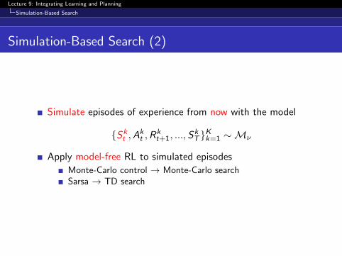
Simulation-Based Search (2)

Simulate episodes of experience from now with the model

{Skt ,A

kt ,R

kt+1, ...,S

kT}Kk=1 ∼Mν

Apply model-free RL to simulated episodes

Monte-Carlo control → Monte-Carlo searchSarsa → TD search



Monte-Carlo Search

Monte-Carlo Simulation

Given a parameterized model Mν and a simulation policy π

Simulate K episodes from current state St

{Skt = St ,A

kt ,R

kt+1, S

kt+1, ...,S

kT}Kk=1 ∼Mν , π

Evaluate state by mean return (Monte-Carlo evaluation)

V (St) =1

K

K∑k=1

G kt

P V π(St)



Monte-Carlo Search

Monte-Carlo Tree Search (Evaluation)

Given a model Mν

Simulate K episodes from current state St using currentsimulation policy π

{Skt = St ,A

kt ,R

kt+1, S

kt+1, ...,S

kT}Kk=1 ∼Mν , π

Build a search tree containing visited states and actions

Evaluate states Q(s, a) by mean return of episodes from s, a

Q(s, a) =1

N(s, a)

K∑k=1

T∑u=t

1(Sku ,A

ku = s, a)Gu

P Qπ(s, a)

After search is finished, select current (real) action withmaximum value in search tree

at = argmaxa∈A

Q(St , a)



Monte-Carlo Search

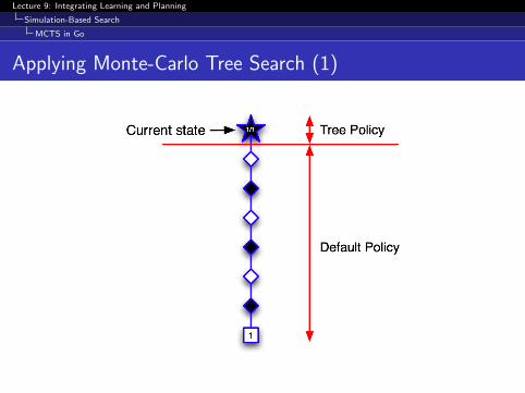
Monte-Carlo Tree Search (Simulation)

In MCTS, the simulation policy π improves

The simulation policy π has two phases (in-tree, out-of-tree)

Tree policy (improves): pick actions from Q(s, a)(e.g. ε− greedy(Q(s, a)))Default policy (fixed): pick actions randomly

Repeat (for each simulated episode)

Select actions in tree according to tree policy.Expand search tree by one nodeRollout to termination with default policyUpdate action-values Q(s,a) in the tree

Output best action when simulation time runs out.

With some assumptions, converges to the optimal values,Q(s, a)→ Q∗(s, a)



MCTS in Go

Case Study: the Game of Go

The ancient oriental game ofGo is 2500 years old

Considered to be the hardestclassic board game

Considered a grandchallenge task for AI(John McCarthy)

Traditional game-tree searchhas failed in Go



MCTS in Go

Rules of Go

Usually played on 19x19, also 13x13 or 9x9 board

Simple rules, complex strategy

Black and white place down stones alternately

Surrounded stones are captured and removed

The player with more territory wins the game



MCTS in Go

Position Evaluation in Go

How good is a position s?

Reward function (undiscounted):

Rt = 0 for all non-terminal steps t < T

RT =

{1 if Black wins0 if White wins

Policy π = 〈πB , πW 〉 selects moves for both players

Value function (how good is position s):

V π(s) = Eπ [RT | s] = P [Black wins | s]

V ∗(s) = maxπB

minπW

V π(s)



MCTS in Go

Monte-Carlo Evaluation in Go

Current position s

Simulation

1 1 0 0 Outcomes

V(s) = 2/4 = 0.5



MCTS in Go

Applying Monte-Carlo Tree Search (1)



MCTS in Go




MCTS in Go

Advantages of MC Tree Search

Highly selective best-first search

Evaluates states dynamically (unlike e.g. DP)

Uses sampling to break curse of dimensionality

Works for “black-box” models (only requires samples)

Computationally efficient, anytime, parallelisable



MCTS in Go

Example: MC Tree Search in Computer Go

Jul 06 Jan 07 Jul 07 Jan 08 Jul 08 Jan 09 Jul 09 Jan 10 Jul 10 Jan 11

MoGo

MoGo

MoGoCrazyStone

CrazyStone

Fuego

Zen

Zen

Zen

Zen

Erica

GnuGo*

GnuGo*

ManyFaces*

ManyFaces

ManyFaces

ManyFaces

ManyFaces

ManyFaces

ManyFaces

Aya*

Aya*

Aya

Aya

Aya

Aya

Indigo

10 kyu

9 kyu

8 kyu

7 kyu

6 kyu

5 kyu

4 kyu

3 kyu

2 kyu

1 kyu

1 dan

2 dan

3 dan

4 dan

5 dan

Foo

1

lecture 9: integrating learning and planning - joseph …josephmodayil.com/uclrl/dyna.pdf · from...

Documents