1

Takashi Yamano

Fall Semester 2005

Lecture Notes on Advanced Econometrics

Lecture 8: Instrumental Variables Estimation

Endogenous Variables

Consider a population model:

y1 = $y2 y2 + $1 + $2 x2 + … + $k-1 x k-1 + u (7-1)

We call y2 an endogenous variable when y2 is correlated with u. As we have studied

earlier, y2 would be correlated with u if (a) there are omitted variables that are correlated

with y2 and y1, (b) y2 is measured with errors, and (c) y1 and y2 are simultaneously

determined (we will cover this issue in the next lecture note). All of these problems, we

can identify the source of the problems as the correlation between the error term and one

or some of the independent variables.

For all of these problems, we can apply instrumental variables (IV) estimations because

instrumental variables are used to cut correlations between the error term and

independent variables. To conduct IV estimations, we need to have instrumental

variables (or instruments in short) that are (R1) uncorrelated with u but (R2) partially

and sufficiently strongly correlated with y2 once the other independent variables are

controlled for.

It turns out that finding proper instruments is very difficult!

In practice, we can test the second requirement (b), but we can not test the first

requirement (a) because u is unobservable. To test the second requirement (b), we need

to express a reduced form equation of y2 with all of exogenous variables. Exogenous

variables include all of independent variables that are not correlated with the error term

and the instrumental variable, z. The reduced form equation for y2 is

y2 = Zδ z + 1δ + 2δ x2 + … + 1−kδ x k-1 + u

For the instrumental variable to satisfy the second requirement (R2), the estimated

coefficient of z must be significant.

In this case, we have one endogenous variable and one instrumental variable. When we

have the same number of endogenous and instrumental variables, we say the endogenous

variables are just identified. When we have more instrumental variables than

endogenous variables, we say the endogenous variables are over-identified. In this case,

2

we need to use “two stage least squares” (2SLS) estimation. We will come back to 2SLS

later.

Define x = (y2, 1, x2, …, xk-1) as a 1-by-k vector, z = (z, 1, x2, …, xk-1) a 1-by-k vector of

all exogenous variables, X as a n-by-k matrix that includes one endogenous variable and

k-1 independent variables, and Z as a n-by-k matrix that include one instrumental

variable and (k-1) independent variables:

=

=

−

−

−

−

−

−

132

1223222

1113121

1322

12232222

11131212

1

1

1

,

1

1

1

nknnn

k

k

nknnn

k

k

xxxz

xxxz

xxxz

Z

xxxy

xxxy

xxxy

X .

The instrumental variables (IV) estimator is

YZXZIV′′= −1)(β (7-2)

Notice that we can take the inverse of Z'X because both Z and X are n-by-k matrices and

Z'X is a k-by-k matrix which has full rank, k. This indicates that there is no perfect co

linearity in Z. The condition that Z'X has full rank of k is called the rank condition.

The consistency of the IV estimators can be shown by using the two requirements for IVs:

)()(ˆ 1 uXZXZIV +′′= − ββ

uZXZ ′′+= −1)(β

nuZnXZ /)/( 1 ′′+= −β

From the first requirement (R1), 0/lim →′ nuZp .

From the second requirement (R2), ).(,/lim xzEAwhereAnXZp ′≡→′

Therefore, the IV estimator is consistent when IVs satisfy the two requirements.

A Bivariate IV model

Let’s consider a simple bivariate model:

y1 = $y2 y2 + $1 + u

We suspect that y2 is an endogenous variable, cov(y2, u) ≠ 0. Now, consider a variable, z,

which is correlated x but not correlated with u: cov(z, y2) ≠ 0 but cov(z, u) = 0. And

consider cov(z, y1):

cov(z, y1) = cov(z, $y2 y2 + $1 + u)

= $y2 cov(z, y2) + cov(z, u)

3

Because cov(z, u) = 0,

$y2 = cov(z, y1) / cov(z, y2)

=

∑

∑

=

=

−−

−−

n

i

ii

n

i

ii

yyzz

yyzz

1

22

1

11

)()(

)()(

The problem in practice is the first requirement, cov(z, u) = 0. We can not empirically

confirm this requirement because u cannot be observed. Thus, the validity of this

assumption is left to economic theory or economists’ common sense.

Recent studies show that even the first requirement can be problematic when the

correlation between the endogenous and instrumental variables is weak. Here is a

bivariate case.

Weak Correlation between the IVs and the Endogenous Variables

In a bivariate model, we write

plim ),cov(

),cov(ˆ

2yz

uzIV += ββ

because Corr(z,u)=cov(z,u)/[sd(z)sd(u)] (see Wooldridge pp714)

plim ))()(/(),(

))()(/(),(ˆ

22 ysdzsdyzcorr

usdzsduzcorrIV += ββ

plim )(

)(

),(

),(ˆ 2

2 usd

ysd

yzcorr

uzcorrIV += ββ

Thus if z is only weakly correlated with the endogenous variable, y2, --corr(z, y2) is very

small-- , the IV estimator could be severely biased.

Example 7-1: Card (1995), CARD.dta.

A dummy variable grew up near a 4 year collage as an IV on educ.

OLS . reg lwage educ Source | SS df MS Number of obs = 3010 ---------+------------------------------ F( 1, 3008) = 329.54 Model | 58.5153536 1 58.5153536 Prob > F = 0.0000 Residual | 534.126258 3008 .17756857 R-squared = 0.0987

4

---------+------------------------------ Adj R-squared = 0.0984 Total | 592.641611 3009 .196956335 Root MSE = .42139 ------------------------------------------------------------------------------ lwage | Coef. Std. Err. t P>|t| [95% Conf. Interval] ---------+-------------------------------------------------------------------- educ | .0520942 .0028697 18.153 0.000 .0464674 .057721 _cons | 5.570883 .0388295 143.470 0.000 5.494748 5.647017 ------------------------------------------------------------------------------ Correlation between nearc4 (an IV) and educ . reg educ nearc4 Source | SS df MS Number of obs = 3010 ---------+------------------------------ F( 1, 3008) = 63.91 Model | 448.604204 1 448.604204 Prob > F = 0.0000 Residual | 21113.4759 3008 7.01910767 R-squared = 0.0208 ---------+------------------------------ Adj R-squared = 0.0205 Total | 21562.0801 3009 7.16586243 Root MSE = 2.6494 ------------------------------------------------------------------------------ educ | Coef. Std. Err. t P>|t| [95% Conf. Interval] ---------+-------------------------------------------------------------------- nearc4 | .829019 .1036988 7.994 0.000 .6256913 1.032347 _cons | 12.69801 .0856416 148.269 0.000 12.53009 12.86594 ------------------------------------------------------------------------------

Thus, nearc4 satisfies the one of the two requirements to be a good candidate as an IV.

IV Estimation: . ivreg lwage (educ=nearc4) Instrumental variables (2SLS) regression Source | SS df MS Number of obs = 3010 ---------+------------------------------ F( 1, 3008) = 51.17 Model | -340.111443 1 -340.111443 Prob > F = 0.0000 Residual | 932.753054 3008 .310090776 R-squared = . ---------+------------------------------ Adj R-squared = . Total | 592.641611 3009 .196956335 Root MSE = .55686 ------------------------------------------------------------------------------ lwage | Coef. Std. Err. t P>|t| [95% Conf. Interval] ---------+-------------------------------------------------------------------- educ | .1880626 .0262913 7.153 0.000 .1365118 .2396134 _cons | 3.767472 .3488617 10.799 0.000 3.08344 4.451504 ------------------------------------------------------------------------------ Instrumented: educ Instruments: nearc4 ------------------------------------------------------------------------------

Note that you can obtain the same coefficient by estimating OLS on lwage with the predicted educ (predicted by nearc4). However, the standard error would be incorrect. In the above IV Estimation, the standard error is already corrected.

End of Example 7-1

5

The Two-Stage Least Squares Estimation

Again, let’s consider a population model:

y1 = $y2 y2 + $1 + $2 x2 + … + $k-1 x k-1 + u (7-3)

where y2 is an endogenous variable. Suppose that there are m instrumental variables.

Instruments, z = (1, x2, …, xk-1, z1,…, zm), are correlated with y2. From the reduced form

equation of y2 with all exogenous variables (exogenous independent variables plus

instruments), we have

y2 = δ1 + δ2 x2 + … + δk-1 x k-1 + δk z1 + … + δk+m-1 zm + ry2 (7-4)

= 2y + ry2

2y is a linear projection of y2 with all exogenous variables. Because 2y is projected with

all exogenous variables that are not correlated with the error term, u, in (7-3), 2y is not

correlated with u, while ry2 is correlated with u. Thus, we can say that by estimating y2

with all exogenous variables, we have divided into two parts: one is correlated with u and

the other is not.

The projection of y2 with Z can be written as

2

1

2 )(ˆˆ yZZZZZy ′′== −δ

When we use the two-step procedure (as we discuss later), we use this 2y in the place of

y2. But now, we treat y2 as a variable in X and project X itself with Z:

XPXZZZZZX Z=′′=Π= −1)(ˆˆ

Π is a (k+m-1)-by-k matrix with coefficients, which should look like:

=Π

−+ 000

010

001

ˆ

1

2

1

mkδ

δ

δ

.

Thus, y2 in X should be expressed as a linear projection, and other independent variables

in X should be expressed by itself. ZZZZPZ′′= −1)( is a n-by-n symmetric matrix and

idempotent (i.e., ZZZ PPP =′ ). We use X as instruments for X and apply the IV estimation

as in

YZZZZXXZZZZXYPXXPXYXXX ZZSLS′′′′′′=′′=′′= −−−−− 11111

2 )())(()(ˆ)ˆ(β (7-5)

6

This can be also written as

YXXXSLS′′= − ˆ)ˆˆ(ˆ 1

2β (7-6)

This is the 2SLS estimator. It is called as two-stage because it looks like we tale two

steps by creating projected X to estimate 2SLS estimator in (10-6). As matter of a fact,

we do not need to take two steps, as you can see in (10-6), we can just estimate 2SLS

estimators in one step by using X and Z. (This is what econometrics packages do.)

The Two-Step procedure

It is still a good idea to know how to estimate the 2SLS estimators by a two-step

procedure:

Step 1: Obtain 2y by estimating an OLS against all of exogenous variables, including all

of instruments (the first-stage regression)

Step 2: Use 2y in the place of y2 to estimate y1 against 2y and all of exogenous

independent variables, not instruments (the second stage regression)

The estimated coefficients from the two-step procedure should exactly the same as 2SLS

from (10-5) or (10-6). However, you must be aware that the standard errors from

the two-step procedure are incorrect, usually smaller than the correct ones. Thus, in

practice, it is always safe not to use the two-step procedure.

Avoid using predicted variables as much as you can!

Econometric packages will provide you 2SLS results based on (10-5) or (10-6). So you

do not need to use the two-step procedure.

We use the first step procedure to test the second requirement for IVs. In the first stage

regression, we should conduct a F-test on all instruments to see if instruments are jointly

significant in the endogenous variable, y2. As we discuss later, instruments should be

strongly correlated with y2 to have reliable 2SLS estimators.

Consistency of 2SLS

Assumption 2SLS.1: For some 1-by-(k+m-1) vector z, E(z'u)=0,

where z = (1, x2, …, xk-1, z1,…, zm).

Assumption 2SLS.2: (a) rank E(z'z) = k+m-1; (b) rank E(z'x) = k.

(b) is the rank condition for identification that z is sufficiently linearly related to

x so that rank E(z'x) has ful column rank.

The order condition is k-1+m≥ k-1+h, where h is the number of endogenous variable.

Thus, the order condition indicates that we must have at least as many instruments as

endogenous variables.

7

Under assumption 2SLS1 and 2SLS2, the 2SLS estimators in (10-5) are consistent.

Under homoskedasticity,

1

1

112 )ˆˆ(ˆ)()ˆˆ(ˆ −

=

−− ′−=′ ∑ XXuknXXn

i

iσ

is a valid estimator of the asymptotic variance of SLS2β .

Under heteroskedasticity, the heteroskedasticity-robust (White) standard errors is

11)ˆˆ(ˆˆˆ)ˆˆ(−− ′Σ′ XXXXXX

Here are some tests for IV estimation. See Wooldridge (Introductory Econometrics) for

details.

Testing for Endogeneity

(i) Estimate the reduced form model using the endogenous variable as the

dependent variable: q against z’s and x’s.

(ii) Obtain the residual, vhat

(iii) Estimate

y = $0 + $1 q + $2 x1 + … + $k-1 x k-1 + $v vhat + u

(iv) If $v is significant, then q is endogenous.

Testing the Over-Identification

(i) Estimate $IV and obtain vhat.

(ii) Regress vhat on z’s and x’s.

(iii) Get R2 and get NR

2, which is chi-squared.

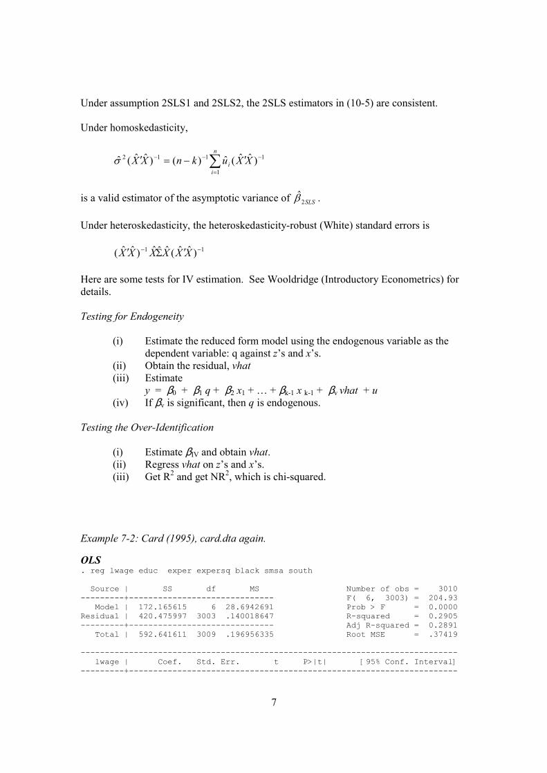
Example 7-2: Card (1995), card.dta again.

OLS . reg lwage educ exper expersq black smsa south Source | SS df MS Number of obs = 3010 ---------+------------------------------ F( 6, 3003) = 204.93 Model | 172.165615 6 28.6942691 Prob > F = 0.0000 Residual | 420.475997 3003 .140018647 R-squared = 0.2905 ---------+------------------------------ Adj R-squared = 0.2891 Total | 592.641611 3009 .196956335 Root MSE = .37419 ------------------------------------------------------------------------------ lwage | Coef. Std. Err. t P>|t| [95% Conf. Interval] ---------+--------------------------------------------------------------------

8

educ | .074009 .0035054 21.113 0.000 .0671357 .0808823 exper | .0835958 .0066478 12.575 0.000 .0705612 .0966305 expersq | -.0022409 .0003178 -7.050 0.000 -.0028641 -.0016177 black | -.1896316 .0176266 -10.758 0.000 -.2241929 -.1550702 smsa | .161423 .0155733 10.365 0.000 .1308876 .1919583 south | -.1248615 .0151182 -8.259 0.000 -.1545046 -.0952184 _cons | 4.733664 .0676026 70.022 0.000 4.601112 4.866217 ------------------------------------------------------------------------------

IV Estimation: nearc2 nearc4 as IVs . ivreg lwage (educ= nearc2 nearc4) exper expersq black smsa south Instrumental variables (2SLS) regression Source | SS df MS Number of obs = 3010 ---------+------------------------------ F( 6, 3003) = 110.30 Model | 86.2368644 6 14.3728107 Prob > F = 0.0000 Residual | 506.404747 3003 .168632949 R-squared = 0.1455 ---------+------------------------------ Adj R-squared = 0.1438 Total | 592.641611 3009 .196956335 Root MSE = .41065 ------------------------------------------------------------------------------ lwage | Coef. Std. Err. t P>|t| [95% Conf. Interval] ---------+-------------------------------------------------------------------- educ | .1608487 .0486291 3.308 0.001 .065499 .2561983 exper | .1192111 .0211779 5.629 0.000 .0776865 .1607358 expersq | -.0023052 .0003507 -6.574 0.000 -.0029928 -.0016177 black | -.1019727 .0526187 -1.938 0.053 -.205145 .0011996 smsa | .1165736 .0303135 3.846 0.000 .0571363 .1760109 south | -.0951187 .0234721 -4.052 0.000 -.1411418 -.0490956 _cons | 3.272103 .8192562 3.994 0.000 1.665743 4.878463 ------------------------------------------------------------------------------ Instrumented: educ Instruments: nearc2 nearc4 + exper expersq ... south ------------------------------------------------------------------------------ . ivreg lwage (educ= nearc2 nearc4 fatheduc motheduc) exper expersq black sms > a south Instrumental variables (2SLS) regression Source | SS df MS Number of obs = 2220 ---------+------------------------------ F( 6, 2213) = 83.66 Model | 108.419483 6 18.0699139 Prob > F = 0.0000 Residual | 320.580001 2213 .144862178 R-squared = 0.2527 ---------+------------------------------ Adj R-squared = 0.2507 Total | 428.999484 2219 .193330097 Root MSE = .38061 ------------------------------------------------------------------------------ lwage | Coef. Std. Err. t P>|t| [95% Conf. Interval] ---------+-------------------------------------------------------------------- educ | .1000713 .01263 7.923 0.000 .0753034 .1248392 exper | .0989441 .009482 10.435 0.000 .0803496 .1175385 expersq | -.002449 .0004013 -6.103 0.000 -.0032359 -.0016621 black | -.1504635 .0259113 -5.807 0.000 -.2012765 -.0996505 smsa | .150854 .0195975 7.698 0.000 .1124226 .1892854 south | -.1072406 .0180661 -5.936 0.000 -.1426688 -.0718123 _cons | 4.26178 .216812 19.657 0.000 3.836604 4.686956 ------------------------------------------------------------------------------ Instrumented: educ Instruments: nearc2 nearc4 fatheduc motheduc + exper expersq ... south ------------------------------------------------------------------------------

9

IV Estimation: fatheduc motheduc as IVs . ivreg lwage (educ= fatheduc motheduc) exper expersq black smsa south Instrumental variables (2SLS) regression Source | SS df MS Number of obs = 2220 ---------+------------------------------ F( 6, 2213) = 83.44 Model | 108.477154 6 18.0795257 Prob > F = 0.0000 Residual | 320.52233 2213 .144836118 R-squared = 0.2529 ---------+------------------------------ Adj R-squared = 0.2508 Total | 428.999484 2219 .193330097 Root MSE = .38057 ------------------------------------------------------------------------------ lwage | Coef. Std. Err. t P>|t| [95% Conf. Interval] ---------+-------------------------------------------------------------------- educ | .099931 .012756 7.834 0.000 .0749161 .124946 exper | .098884 .0095123 10.395 0.000 .0802299 .117538 expersq | -.0024487 .0004012 -6.103 0.000 -.0032356 -.0016619 black | -.1505902 .0259598 -5.801 0.000 -.2014983 -.0996822 smsa | .1509271 .0196181 7.693 0.000 .1124553 .1893988 south | -.1072797 .0180714 -5.936 0.000 -.1427183 -.071841 _cons | 4.26415 .2189075 19.479 0.000 3.834865 4.693436 ------------------------------------------------------------------------------ Instrumented: educ Instruments: fatheduc motheduc + exper expersq ... south ------------------------------------------------------------------------------

Which ones are better?

End of Example 7-2

10

Lecture 9: Heteroskedasticity and Robust Estimators

In this lecture, we study heteroskedasticity and how to deal with it. Remember that we

did not need the assumption of Homoskedasticity to show that OLS estimators are

unbiased under the finite sample properties and consistency under the asymptotic

properties. What matters is how to correct OLS standard errors.

Heteroskedasticity

In this section, we consider heteroskedasticity, while maintaining the assumption of no-

autocorrelation. The variance of disturbance i, ui, is not constant across observations but

not correlated with uj:

Σ=

=

=′

2

2

2

2

1

21

22212

12111

00

00

00

)()()(

)()()(

)()()(

)(

nnnnn

n

n

uuEuuEuuE

uuEuuEuuE

uuEuuEuuE

uuE

σ

σ

σ

or

Ω=

=′ 2

22

22

2

22

1

2

/00

0/0

00/

)( σ

σσ

σσ

σσ

σ

n

uuE

Notice that under homoskedasticity, I=Ω .

Under heteroskedasticity, the sample variance of OLS estimator (under finite sample

properties) is

Var( Β ) = Var [%%%% + (XttttX)-1 Xttttu]

= E [(XttttX)-1 Xttttu uttttX (XttttX)

-1]

= (XttttX)-1 Xtttt E [u utttt] X (XttttX)

-1

= (XttttX)-1 XttttF2S X (XttttX)

-1

= (XttttX)-1 XttttGGGG X (XttttX)

-1 (7-1)

(See Theorem 10.1 in Greene (2003))

11

Unless you specify, however, econometric packages automatically assume

homoskedasticity and will calculate the sample variance of OLS estimator based on the

homoskedasticity assumption:

Var( Β ) = F2 (XttttX)

-1

Thus, in the presence of heteroskedasticity, the statistical inference based on s2(XttttX)

-1

would be biased, and t-statistics and F-statistics are inappropriate. Instead, we should use

(7-1) to calculate standard errors and other statistics.

Finite Sample Properties of OLS Estimators

The OLS estimators are unbiased and have the sampling variance specified in

(6-1). If u is normally distributed, then the OLS estimators are also normally

distributed:

]))(()(,[~|ˆ 112 −− ′Ω′′Β XXXXXXBNX σ

Asymptotic Properties of OLS Estimators

If Q = plim(XttttX) and plim(XttttΩΩΩΩX/ n) are both finite positive definite matrices,

then Β is consistent for B. Under the assumed conditions,

plim Β = B.

(See Greene (2003), page 193-194, for details.)

Robust Standard Errors

If GGGG is known, we can obtain efficient least square estimators and appropriate statistics by

using formulas identified above. However, as in many other problems, GGGG is unknown.

One common way to solve this problem is to estimate GGGG empirically: First, estimate an

OLS model, second, obtain residuals, and third, estimate GGGG:

=Σ

2

2

2

2

1

ˆ00

0ˆ0

00ˆ

ˆ

nu

u

u

(We may multiply this by (n/(n-k-1)) as a degree-of-freedom correction. But when the

number of observations, n, is large, this adjustment does not make any difference.)

Thus by using the estimated GGGG, we have

12

=

′=Σ′ ∑=

2

1

2

212

121

2

1

1

2

2

2

2

2

1

ˆ

ˆ00

0ˆ0

00ˆ

ˆ

kiikn

iii

kiiiii

n

i

i

n xxx

xxx

xxxxx

uX

u

u

u

XXX .

Therefore, we can estimate the variances of OLS estimators (and standard errors) by

using ∑ :

Var( Β ) = (XttttX)-1 Xtttt Σ X (XttttX)

-1 (7-2)

Standard errors based on this procedure are called (heteroskedasticity) robust standard

errors or White-Huber standard errors. Or it is also known as the sandwich

estimator of variance (because of how the calculation formula looks like). This

procedure is reliable but entirely empirical. We do not impose any assumptions on the

structure of heteroskedasticity.

Sometimes, we may impose assumptions on the structure of the heteroskedasticity. For

instance, if we suspect that the variance is homoskedastic within a group but not across

groups, then we obtain residuals for all observations and calculate average residuals for

each group. Then, we have Σ which has a constant 2ˆju for group j. (In STATA, you can

specify groups by using cluster.)

In practice, we usually do not know the structure of heteroskedasticity. Thus, it is safe to

use the robust standard errors (especially when you have a large sample size.) Even if

there is no heteroskedasticity, the robust standard errors will become just conventional

OLS standard errors. Thus, the robust standard errors are appropriate even under

homoskedasticity.

A heteroskedasticity-robust t statistic can be obtained by dividing an OSL estimator by

its robust standard error (for zero null hypotheses). The usual F-statistic, however, is

invalid. Instead, we need to use the heteroskedasticity-robust Wald statistic. Suppose the

hypotheses can be written as

H0: RB = r

Where R is a q x (k+1) matrix (q < (k+1)) and r is a q x 1 vector with zeros for this case.

Thus,

[ ]

==

= −+×

0

0

0

,0:

0010

00010

00001

)1( rIR qkqq .

13

The heteroskedasticity-robust Wald statistics for testing the null hypothesis is

)ˆ()ˆ()ˆ( 1 rRRVRrRW −′′−= − ββ

where V is given in (7-2). The heteroskedasticity-robust Wald statistics is asymptotically

distributed chi-squared with q degree of freedom. The Wald statistics can be turned into

an appropriate F-statistics (q, q-k-1 ) by dividing it by q.

Tests for Heteroskedasticity When should we use robust standard errors? My personal answer to this question is “almost always.” As you will see in Example 7-1, it is very easy to estimate robust standard errors with STATA or other packages. Thus, at least I suggest that you estimate robust standard errors and see if there are any significant differences between conventional standard errors and robust standard errors. If results are robust, i.e., when you do not find any significant differences between two sets of standard errors, then you could be confident in your results based on homoskedasticity. Statistically, you can use following two heteroskedasticity tests to decide if you have to use robust standard errors or not. The Breusch-Pagan Test for Heteroskedasticity

If the homoskedasticity assumption is true, then the variance of error terms should be

constant. We can make this assumption as a null hypothesis:

H0: E(u| X) = F2

To test this null hypothesis, we estimate

2u = *0 + *1 x1 + *2 x2 + … + *k xk + e. (7-3)

Under the null hypothesis, independent variables should not be jointly significant. The F-

statistics that test a joint significance of all independent variables is

)1/()1(

/2

2

1, −−−=−−

knR

kRF knk

The LM test statistics is

LM = n R2 ~ P2

k

The White Test for Heteroskedasticity

14

White proposed to add the squares and cross products of all independent variables to (9-

2):

vxxxxxxxxxxxxu kkkkkk +++++++++++++= −1312211

22

22

2

1122110

2 .........ˆ φφφλλλδδδδ

Because y includes all independent variables, this test is equivalent of conducting the

following test:

vyyu +++= 2

210

2 ˆˆˆ δδδ

We can use F-test or LM-test on H: 00 21 == δδ and .

Example7-1: Step-by-Step Estimation for Robust Standard Errors

In the following do-file, I first estimate a wage model:

logwage = $0 + $1 female + $2 educ + $2 exper + $2 expersq + u

by using WAGE1.dta. Then, by using residuals from this conventional OLS, I estimate

Σ and obtain robust standard errors by step-by-step with matrix. Finally, I verify what I

get with robust standard errors provided by STATA. Of course, you do not need to use

matrix to obtain robust standard errors. You just need to use STATA command,

“robust,” to get robust standard errors (e.g., reg y x1 x2 x3 x4, robust). But at least

you know how robust standard errors are calculated by STATA.

. *** on WAGE1.dta

. *** This do-file estimates White-Huber robust standard errors . set matsize 800 . clear . use c:\docs\fasid\econometrics\homework\wage1.dta . . * Variable construction . gen logwage=ln(wage) . gen expsq=exper*exper . gen x0=1 . . * Obtain conventional OLS residuals

. reg logwage female educ exper expsq Source | SS df MS Number of obs = 526 ---------+------------------------------ F( 4, 521) = 86.69 Model | 59.2711314 4 14.8177829 Prob > F = 0.0000 Residual | 89.05862 521 .17093785 R-squared = 0.3996 ---------+------------------------------ Adj R-squared = 0.3950 Total | 148.329751 525 .28253286 Root MSE = .41345 ------------------------------------------------------------------------------ logwage | Coef. Std. Err. t P>|t| [95% Conf. Interval] ---------+--------------------------------------------------------------------

15

female | -.3371868 .0363214 -9.283 0.000 -.4085411 -.2658324 educ | .0841361 .0069568 12.094 0.000 .0704692 .0978029 exper | .03891 .0048235 8.067 0.000 .029434 .0483859 expsq | -.000686 .0001074 -6.389 0.000 -.000897 -.0004751 _cons | .390483 .1022096 3.820 0.000 .1896894 .5912767 ------------------------------------------------------------------------------ . predict e, residual . gen esq=e*e . . * Create varaibles with squared residuals . gen efemale=esq*female . gen eeduc=esq*educ . gen eexper=esq*exper . gen eexpsq=esq*expsq . gen ex0=esq*x0 . . * Matrix construction . mkmat logwage, matrix(y) . mkmat efemale eeduc eexper eexpsq ex0, matrix(ex) . . * White-Huber robust standard errors . matrix ixx=syminv(x'*x) . matrix sigma=ex'*x . matrix b_robust=(526/(526-5))*ixx*sigma*ixx . * Here is the White-Huber robust var(b^) . mat list b_robust b_robust[5,5] female educ exper expsq x0 female .00130927 .00003556 -1.277e-07 1.647e-09 -.00109773 educ .00003556 .00005914 -3.028e-06 1.570e-07 -.00077218 exper -1.277e-07 -3.028e-06 .00002186 -4.500e-07 -.00010401 expsq 1.647e-09 1.570e-07 -4.500e-07 1.009e-08 5.805e-07 x0 -.00109773 -.00077218 -.00010401 5.805e-07 .01179363 . * Take square root of the diagonal elements>> sd.error . * Thus sd.er. for female is (0.0013)^.5=0.036, educ is (0.000059)^.5=0.00768, . * and so on.

16

But, you do not need to go through this calculation yourself. STATA has a command

called “robust.” . * Verify with STATA version of robust standard errors . reg logwage female educ exper expsq, robust Regression with robust standard errors Number of obs = 526 F( 4, 521) = 81.97 Prob > F = 0.0000 R-squared = 0.3996 Root MSE = .41345 ------------------------------------------------------------------------------ | Robust logwage | Coef. Std. Err. t P>|t| [95% Conf. Interval] ---------+-------------------------------------------------------------------- female | -.3371868 .0361838 -9.319 0.000 -.4082709 -.2661026 educ | .0841361 .00769 10.941 0.000 .069029 .0992432 exper | .03891 .0046752 8.323 0.000 .0297253 .0480946 expsq | -.000686 .0001005 -6.829 0.000 -.0008834 -.0004887 _cons | .390483 .1085985 3.596 0.000 .1771383 .6038278 ------------------------------------------------------------------------------ end of do-file

End of Example 7-1

Example 7-2: the Breusch-Pagan test

. *** on WAGE1.dta . *** This do-file conducts the Breusch-Pagan heteroskedasticity test . set matsize 800 . clear . use c:\docs\fasid\econometrics\homework\wage1.dta . * Variable construction . gen logwage=ln(wage) . gen expsq=exper*exper . * Obtain residuals from the level model

. reg wage female educ exper expsq (Output is omitted) . predict u, residual . gen uu=u*u . * the BP test . reg uu female educ exper expsq Source | SS df MS Number of obs = 526 ---------+------------------------------ F( 4, 521) = 12.79 Model | 24632.1712 4 6158.0428 Prob > F = 0.0000 Residual | 250826.691 521 481.433189 R-squared = 0.0894 ---------+------------------------------ Adj R-squared = 0.0824 Total | 275458.863 525 524.683548 Root MSE = 21.942 ------------------------------------------------------------------------------ uu | Coef. Std. Err. t P>|t| [95% Conf. Interval] ---------+-------------------------------------------------------------------- female | -5.159055 1.927575 -2.676 0.008 -8.945829 -1.372281 educ | 1.615551 .3691974 4.376 0.000 .8902524 2.340849 exper | 1.067343 .2559852 4.170 0.000 .5644535 1.570233 expsq | -.0189783 .0056986 -3.330 0.001 -.0301733 -.0077833 _cons | -18.15532 5.424263 -3.347 0.001 -28.81144 -7.499208 ------------------------------------------------------------------------------ . test female educ exper expsq

17

( 1) female = 0.0 ( 2) educ = 0.0 ( 3) exper = 0.0 ( 4) expsq = 0.0 F( 4, 521) = 12.79

Prob > F = 0.0000 The LM test statistics is 526 x 0.0894 = 47.02. This is significant at 1 percent level because the critical level is 13.28 for a chi-square distribution of four degree of freedom.

End of Example 7-2

Example 7-3: the White test

. * Obtain residuals from the log model

. reg logwage female educ exper expsq (Output omitted) . predict yhat (option xb assumed; fitted values) . predict v, residual . gen yhatsq=yhat*yhat . gen vsq=v*v . * the White test . reg vsq yhat yhatsq Source | SS df MS Number of obs = 526 ---------+------------------------------ F( 2, 523) = 3.96 Model | .605241058 2 .302620529 Prob > F = 0.0197 Residual | 40.003265 523 .076488078 R-squared = 0.0149 ---------+------------------------------ Adj R-squared = 0.0111 Total | 40.608506 525 .077349535 Root MSE = .27656 ------------------------------------------------------------------------------ vsq | Coef. Std. Err. t P>|t| [95% Conf. Interval] ---------+-------------------------------------------------------------------- yhat | -.187119 .2637874 -0.709 0.478 -.7053321 .331094 yhatsq | .0871914 .0812258 1.073 0.284 -.0723774 .2467603 _cons | .2334829 .2096599 1.114 0.266 -.1783961 .645362 ------------------------------------------------------------------------------ . test yhat yhatsq ( 1) yhat = 0.0 ( 2) yhatsq = 0.0 F( 2, 523) = 3.96 Prob > F = 0.0197 LM stat is 526 x 0.0149 = 7.84, which is significant at 5 percent level but not at 1 percent level.

End of Example 7-3

18

Lecture 10: GLS, WLS, and FGLS Generalized Least Square (GLS)

So far, we have been dealing with heteroskedasticity under OLS framework. But if we

knew the variance-covariance matrix of the error term, then we can make a

heteroskedastic model into a homoskedastic model.

As we defined before

Σ=Ω=′ 2)( σuuE .

Define further that

PP′=Ω−1

P is a “n x n” matrix

Pre-multiply P on a regression model

Py = PXB + Pu

or

y* = X* B + u* (9-1)

In this model, the variance of u* is

E(u* utttt*) = E(PuuttttPtttt) = PE(uutttt)Ptttt= P Ω2σ Ptttt= 2σ P ΩPtttt= 2σ I.

Note that PSPtttt= I, because define PSPtttt=A, then PttttPSPtttt= PttttA, by the definition of P

S-1SPtttt= PttttA, thus Ptttt= PttttA. Therefore, A must be I.

Because E(u* utttt*) = 2σ I, the model (9-3) satisfies the assumption of homoskedasticity.

Thus, we can estimate the model (9-3) by the conventional OLS estimation.

Hence,

**

1

** )(ˆ yXXX ′′=Β −

PyPXPXPX ′′′′= −1)(

yXXX 111 )( −−− Ω′Ω′=

is the efficient estimator of Β . This is called the Generalized Least Square (GLS)

estimator. Note that the GLS estimators are unbiased when E( u*| X* ) = 0. The variance

of GLS estimator is

1121

**

2 )()()ˆvar( −−− Ω′=′=Β XXXX σσ .

Note that, under homoskedasticity, i.e., 1−Ω =I, GLS becomes OLS.

19

The problem is, as usual, that we don’t know ΣΩ or2σ . Thus we have to either assume

Σ or estimate Σ empirically. An example of the former is Weighted Least Squares

Estimation and an example of the later is Feasible GLS (FGLS).

Weighted Least Squares Estimation (WLS)

Consider a general case of heteroskedasticity.

Var(ui) = ii ωσσ 22 = .

Then,

=ΩΩ=

=′

−

−

−

−

1

1

2

1

1

122

1

2

00

00

00

,

00

00

00

)(

nn

thusuuE

ω

ω

ω

σ

ω

ω

ω

σ .

Because of PP′=Ω−1 , P is a n x n matrix whose i-th diagonal element is iω/1 . By

pre-multiplying P on y and X, we get

==

==

nnknnn

k

k

nn xx

xx

xx

PXXand

y

y

y

Pyy

ωωω

ωωω

ωωω

ω

ω

ω

/...//1

/...//1

/...//1

/

/

/

1

222212

111111

*

22

11

* .

The OLS on ** Xandy is called the Weighted Least Squares (WLS) because each

variable is weighted by iω . The question is: where can we find iω ?

Feasible GLS (FGLS)

Instead of assuming the structure of heteroskedasticity, we may estimate the structure of

heteroskedasticity from OLS. This method is called Feasible GLS (FGLS). First, we

estimate Ω from OLS, and, second, we use .ˆ ΩΩ ofinstead

yXXXFGLS

111 ˆ)ˆ(ˆ −−− Ω′Ω′=β

There are many ways to estimate FGLS. But one flexible approach (discussed in

Wooldridge page 277) is to assume that

)...exp()|var( 22110

22

kk xxxuXu δδδδσ ++++==

20

By taking log of the both sides and using 2u instead of 2u , we can estimate

exxxu kk +++++= δδδα ...)ˆlog( 22110

2 .

The predicted value from this model is ∧

= )ˆlog(ˆ 2ug i . We then convert it by taking the

exponential into 22 ˆ))ˆexp(log()ˆexp(ˆ uug ii

∧

===ω . We now use WLS with weights

2ˆ/1ˆ/1 uoriω .

Example 9-1

. * Estimate the log-wage model by using WAGE1.dta with WLS . * Weight is educ . * Generate weighted varaibles . gen w=1/(educ)^0.5 . gen wlogwage=logwage*w . gen wfemale=female*w . gen weduc=educ*w . gen wexper=exper*w . gen wexpsq=expsq*w . * Estimate weighted least squares (WLS) model . reg wlogwage weduc wfemale wexper wexpsq w, noc Source | SS df MS Number of obs = 524 ---------+------------------------------ F( 5, 519) = 1660.16 Model | 113.916451 5 22.7832901 Prob > F = 0.0000 Residual | 7.12253755 519 .013723579 R-squared = 0.9412 ---------+------------------------------ Adj R-squared = 0.9406 Total | 121.038988 524 .230990435 Root MSE = .11715 ------------------------------------------------------------------------------ wlogwage | Coef. Std. Err. t P>|t| [95% Conf. Interval] ---------+-------------------------------------------------------------------- weduc | .080147 .006435 12.455 0.000 .0675051 .0927889 wfemale | -.3503307 .0354369 -9.886 0.000 -.4199482 -.2807133 wexper | .0367367 .0045745 8.031 0.000 .0277498 .0457236 wexpsq | -.0006319 .000099 -6.385 0.000 -.0008264 -.0004375 w | .4557085 .0912787 4.992 0.000 .2763872 .6350297 ------------------------------------------------------------------------------

End of Example 9-1

Example 9-2

. * Estimate reg . reg logwage educ female exper expsq (Output omitted) . predict e, residual . gen logesq=ln(e*e)

21

. reg logesq educ female exper expsq (output omitted) . predict esqhat (option xb assumed; fitted values) . gen omega=exp(esqhat) . * Generate weighted varaibles . gen w=1/(omega)^0.5 . gen wlogwage=logwage*w . gen wfemale=female*w . gen weduc=educ*w . gen wexper=exper*w . gen wexpsq=expsq*w . * Estimate Feasible GLS (FGLS) model . reg wlogwage weduc wfemale wexper wexpsq w, noc Source | SS df MS Number of obs = 524 ---------+------------------------------ F( 5, 519) = 1569.72 Model | 31164.1981 5 6232.83962 Prob > F = 0.0000 Residual | 2060.77223 519 3.97065941 R-squared = 0.9380 ---------+------------------------------ Adj R-squared = 0.9374 Total | 33224.9703 524 63.406432 Root MSE = 1.9927 ------------------------------------------------------------------------------ wlogwage | Coef. Std. Err. t P>|t| [95% Conf. Interval] ---------+-------------------------------------------------------------------- weduc | .0828952 .0069779 11.880 0.000 .0691868 .0966035 wfemale | -.2914609 .0349884 -8.330 0.000 -.3601971 -.2227246 wexper | .0376525 .004497 8.373 0.000 .0288179 .0464872 wexpsq | -.0006592 .0001008 -6.540 0.000 -.0008573 -.0004612 w | .3848487 .0950576 4.049 0.000 .1981038 .5715936 ------------------------------------------------------------------------------

End of Example 9-2

22

Lecture 11: Unobserved Effects and Panel Analysis

Panel Data

There are two types of panel data sets: a pooled cross section data set and a

longitudinal data set. A pooled cross section data set is a set of cross-sectional data

across time from the same population but independently sampled observations each time.

A longitudinal data set follows the same individuals, households, firms, cities, regions, or

countries over time.

Many governments conduct nationwide cross sectional surveys every year or every once

in a while. Census is an example of such surveys. We can create a pooled cross section

data set if we combine these cross sectional surveys over time. Because these surveys are

often readily available from governments (well this is not true for most of the times

because of many government officials do not see any benefits of making publicly funded

surveys public!), it is relatively easier to obtain pooled cross section data.

Longitudinal data, however, can provide much more detailed information as we see in

this lecture. Because longitudinal data follow the same samples over time, we can

analyze behavioral changes over time of the samples.

Nonetheless, pooled cross section data can provide information that a single cross section

data cannot.

Pooled Cross Section Data

With pooled cross section data, we can examine changes in coefficients over time. For

instance,

yit = $0 + $1 Tit + $2 xit1 + $3 xit2 + $4 xit3 + uit (1)

t = 1, 2

i = 1, 2,…, N1, N1+1, N1+2,…, N1+N2

where Tit = 1 if t = 2 and dit = 0 if t = 1.

The coefficient of the time dummy Tit measures a change in the constant term over time.

If we are interested in a change in a potential effect of one of the variables, then we can

use an interaction term between the time dummy and one of the variables:

yit = $0 + $1 dit + $2 xit1 + *2 (Tit ×xit1 ) + $3 xit2 + $4 xit3 + uit (2)

*2 measures a change in the coefficient of x1 over time.

How about if there are changes in all of the coefficients over time? To examine if there is

a structural change, we can use the Chow test. To conduct the Chow test, consider the

following model:

23

yit = $0 + $1 xit1 + $2 xit2 + $3 xit3 + $4 xit4 + uit (3)

for t = 1 , 2.

We consider this model as a restricted model because we are imposing restrictions that

all the coefficients remain the same over time. There are k+1 restrictions (in this case 5

restrictions).

Unrestricted models are

yit = *0 + *1 xit1 + *2 xit2 + *3 xit3 + *4 xit4 + vit for t = 1 (4)

and

yit = (0 + (1 xit1 + (2 xit2 + (3 xit3 + (4 xit4 + eit for t = 2 (5)

The coefficients of the first model (t = 1) are not restricted to be the same as in the second

model (t = 2). If all of the coefficients remain the same over time, i.e., $j = *j = (j, then

the sum of squared residuals from the restricted model (SSRr) should be equal to the sum

of the sums of squared residuals from the two unrestricted models (SSRur1 + SSRur2).

On the other hand, if there is a structural change, i.e., changes in the coefficients over

time, then the sum of SSRur1 and SSRur2 should be smaller than SSRr, because

unrestricted coefficients in unrestricted models should match the data more precisely than

the restricted model. Then we take the difference between SSRr and (SSRur1 + SSRur2)

and examine if there is statistically significant difference between the two:

)]1(2[/)(

)1(/)]([

2111

21

+−++

++−=

kNNSSRSSR

kSSRSSRSSRF

urur

ururr

This is called the Chow test.

Alternatively, we can create interaction terms on all of independent variables (including

the constant term) and conduct a F-test on the coefficients of the k+1 interaction terms.

This is just the same the Chow test.

Difference-in-Differences Estimator

In many economic analyses, we are interested in some of policy variables or politically

interesting variables and how these variables affect people’s lives. However, evaluating

24

the impacts of various policies is difficult because most of policies are not done under

experimental designs.

For instance, suppose a government of a low-income country decided to invest in health

facilities to improve child health. Suppose this particular government decided to start

with the most-needy communities. After some years, the government wanted to evaluate

the impacts of the investment in health facilities. The government conducts a cross-

sectional survey. However, the government finds negative correlation between newly-

build health facilities and child health. What happened?

Child health

Communities without E(HT2: z = 0)

E(HT2: z = 1)

* Communities

with investments

Time

1 2

The problem is that the government built health facilities in communities with poor child

health.

In the figure above, the child health in poor community i with the government-

investments (z) has improved over time, but its absolute level is still not as good as the

child health in rich communities without the government investments. Thus, an OLS

model with a dummy variable for the government investments in health facilities will

find a coefficient of z:

Hit = $0 + $1 z it + uit (6)

for i = 1, …, N communities.

When we find a negative coefficient or an opposite effect of what expected, we call it the

reverse causality.

From the figure, it is obvious that we need to measure a difference between the two

groups for each time period and measure a net change in the differences over time:

* = [E(Hi2:z =1)–E(Hi2:z =0)] – [E(Hi1: z =1)–E(Hi2: z =0)]. (7)

25

Although both differences are negative, the difference between the two groups in the

second period is much smaller than the difference in the first period. Thus, the net

change is positive, which measures the net impact of z on H. We call the * in (10-7) the

difference-in-differences (DID) estimator.

The difference-in-differences estimator can be estimated by estimating the following

model:

Hit = $0 + $1 T + $2 z i + * (T ×z i) + uit (8)

We can think this example as a kind of the omitted variables problem. We can rewrite

(9-6) as

Hi = $0 + $1 z i + " i + ui (9)

where " i is an important unobserved variable (or an unobserved fixed effect) which is

correlated with both the government investments and the child health. Let’s say that " i

measures the lack of basic infrastructure in community i: the larger the " i, the poorer the

basic infrastructure. Because the government targets the poor communities for the

investments, " i and zi are correlated positively. But " i and Hi are correlated negatively

because " i measures the lack of basic infrastructure. Therefore, the estimated coefficient

of zi will be biased downward, which produces a reverse causality.

The First Differenced Estimation

Let’s go back to the DID estimator and rearrange it so that the first term measure a

difference in Hit of community i over time:

* = [E(HT2:z =1)–E(HT1:z =1)] – [E(HC2: z =0)–E(HC1: z =0)]. (10)

Here the first term measures a change over time for the treatment group (T) and the

second term measures for the comparison group (C).

In a regression form, we can also rearrange (8). Let’s write the equation (8) with an

unobserved fixed effect:

Hit = $0 + $1 T + $2 z i + * (T ×z i) + " i + uit (11)

Now, the problem is that z could be correlated with " i, which may be also correlated

with Hit. For the first period (thus T = 0), the equation (11) is

Hit = $0 + $2 z i + " i + uit,

and for the second period (T = 1):

26

Hit+1 = ($0 + $1) + ($2 + *) z i + " i + uit+1.

Then by taking the first-difference, we have

Hit+1 - Hit = $0 + * z i + vit+1 (12)

Notice that the unobserved fixed effect, " i, has been excluded from this model because

the unobserved fixed effect is fixed over time. In the first-differenced equation (12), z

will not be correlated with the error term.

Quasi-experimental and Experimental Designs

From this point of view, it is obvious that under a nonrandom assignment of z (or a quasi-

experimental design), * in (8) could be biased because z (a program indicator) could be

correlated with unobserved factors which may be also correlated with H (a dependent

variable).

In contrast, under a random assignment of z (or an experimental design), z will not be

correlated with any of unobserved factors. Thus the difference-in-differences estimator

will provide reliable estimators of the impacts of programs on outcomes.

Under an experimental design, a group of individuals or observations that receive

benefits from a give policy is called a treatment group or an experimental group. And a

group of non-beneficiaries is called a control group. Under a quasi-experimental design,

a group of non-beneficiaries is called a comparison group, and reserve the name “the

control group” for experimental designs.

In social science, it is difficult to conduct experimental designed programs because of

ethics and political difficulties. But experimental designed programs can provide very

useful information about the effectiveness of public (or private) policies.

Recent Example of an experimental designed project: PROGRESA in Mexico, designed

and research by IFPRI. See www.ifpri.org.

For a summary of US experience, see Grossman (1994) “Evaluating social policies:

principles and U.S. experience,” World Bank Research Observer, vol9: 159-80.

Thus, we have dealt with an omitted variable problem by taking a difference over time.

Next, we study the omitted fixed effect problem in general.

The Omitted Variables Problem Revisited

Suppose that a correctly specified regression model would be

27

uXXuXy ++=+= 2211 βββ

X1 and X2 have k1 and k2 columns, respectively. But, suppose we regress y on X1 without

including X2 (X2 represent omitted variables). The OLS estimator is

)()()(ˆ22111

1

111

1

111 uXXXXXYXXX ++′′=′′= −− βββ

uXXXXXXX 1

1

11221

1

111 )()( ′′+′′+= −− ββ

By taking the expectation on both sides, we have

2121221

1

1111ˆ)()ˆ( βδββββ +=′′+= −

XXXXE

Note, however, that the second term indicates the column of slopes ( 12δ ) in least squares

regression of the corresponding column of X2 on the columns of X1.

Thus, unless either 12δ =0 or 2β =0, 1β is biased.

To overcome the omitted variables problem, we can take two different methods. First

method is to use panel data. As you see later, by using panel (longitudinal) data, we can

eliminate unobserved variables that are specific to each sample and fixed (or time-

invariant or time-constant) over time. Second method is to use instrumental variables

that are correlated with independent variables that are considered to be correlated with

unobserved variables but uncorrelated with the dependent variable. We will discuss

instrumental variables in the next lecture note.

Before we discuss about estimation methods that use panel data, let us start with types of

panel data.

Linear Unobserved Effects

What are unobserved variables? It is impossible to collect all variables in surveys that

affect people’s economic activities. Thus, it is inevitable to have unobserved variables in

our estimation models. What, then, we should do? First, we should start with

characterizing possible unobserved variables.

The most common type of unobserved variables is a fixed effect. A fixed effect is a time

invariant characteristic of an individual or a group (or cluster). For instance, ai may

represent a fixed characteristic of group i. This could be a regional fixed effect or a

cluster fixed effect. Another example is aj which represents a fixed characteristic of a

group (cluster) j.

Suppose, we want to estimate the following model with a group fixed effect,

28

yi = $0 + $1 xi1 + … + $k xi k + a j + ui (13)

In this case, as long as unobserved variables (that are correlated with individual variables

and the dependent variable) are fixed characteristics of groups, then we can eliminate the

omitted variables problem by explicitly including group dummies:

yi = $0 + $1 xi1 + … + $k xi k + """"' dj + ui (14)

where """"' is a 1-by-j vector, and dj is a j-by-1 vector. For instance, it is common practice

to include district or village dummies in cross-sectional data. However, in a cross-

sectional data set, it is impossible to include individual dummies for all samples because

we have only one observation per sample. We will have n-1 dummies for n observations.

If we have multiple observations for each sample (thus we need longitudinal data not a

pooled cross-sectional data over time), then it is possible to have n-1 dummies for s x n

observations. (s is the number of observations per sample.) Thus, we estimate

yit = $0 + $1 xit 1 + … + $k xit k + """"' di + uit (15)

This is called the Dummy Variable Regression model. In this model, we have

eliminated the unobserved fixed effects by explicitly including individual dummy

variables.

A different way of eliminating the fixed effects is to use the first difference model, as

we have seen earlier. Here let us reconsider the first difference model in a general

treatment. Suppose, again, that we have the following model for time t=1 and t=2:

yi1 = $0 + $1 xi1 1 + … + $k xi1 k + a j + ui1

and

yi2 = $0 + $1 xi2 1 + … + $k xi2 k + a j + ui2

By subtracting the model for t=1 from the model for t=2, we have

yi2 - yi1 = $1 (xi2 1 - xi1 1) + … + $k (xi2 k - xi1 k) + ui2 - ui1

or

ikiki uxxy ∆+∆++∆=∆ ββ ...11

This is called the first difference model. Notice that the individual fixed effect, a j, has

been eliminated. Thus as long as the new error term is uncorrelated with the new

independent variables, then the estimators should be unbiased.

Some notes: First, a first differenced independent variable, kix∆ , must have some

variation across i. For instance, a gender dummy variable does not change over time, the

first-differenced gender dummy is zero for all i. Thus, you can not estimate coefficient

on time-invariant independent variables in first difference models. Second, differenced

independent variables loose variation. Thus, estimators often have large standard errors.

Large sample size helps to estimate parameters precisely.

29

Fixed Effect Estimation

In the previous lecture, we studied the first differenced model, concerning the correlation

between a policy variable and an unobserved fixed effect. In this lecture, we generalize

the model. Consider the following model with T period and k variables

yit = $0 + $1 xit1 + $2 xit2 + … + $k xit k + " i + uit (16)

The omitted unobserved fixed effect could be correlated with any of k independent

variables.

To take the fixed effect away, one can subtract the mean of each variable:

itikitkiitiit vxxxxyy +−++−=− )(...)( 1111 ββ (17)

As you can see, the unobserved fixed effect has been excluded from the model. This

model is called the fixed effect estimation. To estimate the fixed effect model, you need

to transform each variable by taking the mean out and estimate the OLS with the

transformed data (the time-demeaned data). In STATA, you don’t need to transfer the

data yourself. Instead you just need to use a command “xtreg y x1 x2 … xk, fe i(id).” See

the manuals under “xtreg.”

One drawback of the fixed effect estimation is that some of time-invariant variables will

be also excluded from the model. For instance, consider a typical wage model, where the

dependent variable is log(wage). Some of individual characteristics, such as education

and gender are time-invariant (or fixed over time). Thus if you are interested in the

effects of time-invariant variables you cannot estimate the coefficients of such variables.

However, what you can do is to estimate the changes in the effects of such time-invariant

variables.

Instead of taking the fixed effects out, we can explicitly include them as dummies:

yit = $0 + $1 xit1 + $2 xit2 + … + $k xit k + *1" 1 + … +*n" n + uit (18)

This is called the least squares dummy variable (LSDV) model. The LSDV model

provides the exactly the same results as Fixed Effect model.

When T=2, the first differenced (FD) model, the Fixed Effect (FE) model, and LSDV

model all provide the same results.

30

Example 11-1: OLS, Fixed Effect, First-Differenced, and LSDV models

. use c:\docs\fasid\econometrics\homework\JTRAIN.dta; . keep if year==1988|year==1989; (157 observations deleted) . replace sales=sales/10000; (254 real changes made) . ** OLS; . reg hrsemp grant employ sales union d89; Source | SS df MS Number of obs = 220 ---------+------------------------------ F( 5, 214) = 2.07 Model | 64302349.8 5 12860470.0 Prob > F = 0.0703 Residual | 1.3291e+09 214 6210560.99 R-squared = 0.0461 ---------+------------------------------ Adj R-squared = 0.0239 Total | 1.3934e+09 219 6362385.39 Root MSE = 2492.1 ------------------------------------------------------------------------------ hrsemp | Coef. Std. Err. t P>|t| [95% Conf. Interval] ---------+-------------------------------------------------------------------- grant | 824.4124 419.8616 1.964 0.051 -3.181518 1652.006 employ | -3.411366 4.232316 -0.806 0.421 -11.75373 4.931001 sales | .0431946 .3313198 0.130 0.896 -.6098735 .6962627 union | 942.0082 442.0818 2.131 0.034 70.61581 1813.401 d89 | -287.6238 338.4361 -0.850 0.396 -954.7191 379.4715 _cons | 156.7909 300.7423 0.521 0.603 -436.0056 749.5874 ------------------------------------------------------------------------------ . ** Fixed Effect Model; . xtreg hrsemp grant employ sales union d89, fe i(fcode); Fixed-effects (within) regression Number of obs = 220 Group variable (i) : fcode Number of groups = 114 R-sq: within = 0.0322 Obs per group: min = 1 between = 0.0106 avg = 1.9 overall = 0.0212 max = 2 F(4,102) = 0.85 corr(u_i, Xb) = -0.0144 Prob > F = 0.4972 ------------------------------------------------------------------------------ hrsemp | Coef. Std. Err. t P>|t| [95% Conf. Interval] ---------+-------------------------------------------------------------------- grant | 846.6938 552.6861 1.532 0.129 -249.5565 1942.944 employ | 1.504937 20.69735 0.073 0.942 -39.54816 42.55803 sales | -.0847216 .9174962 -0.092 0.927 -1.904571 1.735128 union | (dropped) d89 | -292.2915 368.5441 -0.793 0.430 -1023.297 438.714 _cons | 137.1313 917.5104 0.149 0.881 -1682.746 1957.009 ------------------------------------------------------------------------------ sigma_u | 1742.3611 sigma_e | 2578.396 rho | .31349012 (fraction of variance due to u_i) ------------------------------------------------------------------------------ F test that all u_i=0: F(113,102) = 0.87 Prob > F = 0.7716

31

. ** LSDV model;

. xi: reg hrsemp grant employ sales union d89 i.fcode; i.fcode Ifcod1-157 (Ifcod1 for fcode==410032 omitted) Source | SS df MS Number of obs = 220 ---------+------------------------------ F(117, 102) = 0.92 Model | 715253529 117 6113278.03 Prob > F = 0.6706 Residual | 678108872 102 6648126.19 R-squared = 0.5133 ---------+------------------------------ Adj R-squared = -0.0449 Total | 1.3934e+09 219 6362385.39 Root MSE = 2578.4 ------------------------------------------------------------------------------ hrsemp | Coef. Std. Err. t P>|t| [95% Conf. Interval] ---------+-------------------------------------------------------------------- grant | 846.6938 552.6861 1.532 0.129 -249.5565 1942.944 employ | 1.504937 20.69735 0.073 0.942 -39.54816 42.55803 sales | -.0847216 .9174962 -0.092 0.927 -1.904571 1.735128 union | -838.5586 5723.478 -0.147 0.884 -12191.05 10513.93 d89 | -292.2915 368.5441 -0.793 0.430 -1023.297 438.714 Ifcod2 | -192.7619 3889.521 -0.050 0.961 -7907.609 7522.085 Ifcod3 | -203.2925 4021.587 -0.051 0.960 -8180.091 7773.506 Output omitted… . ** First Differenced Model; . reg dhrsemp dgrant demploy dsales; Source | SS df MS Number of obs = 106 ---------+------------------------------ F( 3, 102) = 0.81 Model | 32189365.8 3 10729788.6 Prob > F = 0.4928 Residual | 1.3562e+09 102 13296252.1 R-squared = 0.0232 ---------+------------------------------ Adj R-squared = -0.0055 Total | 1.3884e+09 105 13222924.6 Root MSE = 3646.4 ------------------------------------------------------------------------------ dhrsemp | Coef. Std. Err. t P>|t| [95% Conf. Interval] ---------+-------------------------------------------------------------------- dgrant | 846.6938 552.6861 1.532 0.129 -249.5565 1942.944 demploy | 1.504937 20.69735 0.073 0.942 -39.54816 42.55803 dsales | -.0847216 .9174962 -0.092 0.927 -1.904571 1.735128 _cons | -292.2915 368.5441 -0.793 0.430 -1023.297 438.714

End of Example 11-1

Example 11-2: Transferring The Panel Data

In general, the panel data are stacked vertically. For instance, in JTRAIN.dta, two

observations (actually there are three years of observations, but I dropped one year) for

each firm is stacked vertically:

. list fcode year d89 employ firm code year d89 # of employees 1. 410032 1988 0 131 2. 410032 1989 1 123 3. 410440 1988 0 13 4. 410440 1989 1 14 5. 410495 1988 0 25 6. 410495 1989 1 24

32

To construct differenced variables, you need to “linearize” the vertical data. Here is an

example:

. do "C:\WINDOWS\TEMP\STD0c0000.tmp" . #delimit; delimiter now ; . clear; . set more off; . set matsize 800; . set memory 100m; (102400k) . *** Obtain data from 1988; . clear; . use c:\docs\fasid\econometrics\homework\JTRAIN.dta; . keep year fcode employ; . keep if year==1988; (314 observations deleted) . rename employ employ88; . drop year; . sort fcode; . save c:\docs\tmp\jtrain88.dta, replace; file c:\docs\tmp\jtrain88.dta saved . *** Obtain data from 1989; . clear; . use c:\docs\fasid\econometrics\homework\JTRAIN.dta; . keep fcode year employ; . keep if year==1989; (314 observations deleted) . rename employ employ89; . drop year; . sort fcode; . save c:\docs\tmp\jtrain89.dta, replace; file c:\docs\tmp\jtrain89.dta saved . ** Combine the two years; . clear; . use c:\docs\tmp\jtrain89.dta; . sort fcode; . merge fcode using c:\docs\tmp\jtrain88.dta; . gen demploy=employ89-employ88; (11 missing values generated) . list fcode employ89 employ88 demploy in 1/3; fcode employ89 employ88 demploy 1. 410032 123 131 -8 2. 410440 14 13 1 3. 410495 24 25 -1

End of Example 11-2

33

Lecture 12: Random Effect Models and the Hausman Test

Random Effect Estimation

Let’s go back to a general longitudinal model with T periods:

yit = $0 + $1 xit1 + $2 xit2 + … + $k xit k + " i + uit (1)

The purpose of the fixed effect estimation and the first differenced estimation is to

eliminate " i because we suspect " i to be correlated with some of independent variables.

However, what if we are wrong (that there is no correlation between " Ii and any of

independent variables)? If this is case, then the FE and FD estimations will be inefficient

because we lose n-1 degree of freedom (think about having n-1 dummies).

Even when there is no correlation between " i and independent variables, the OLS

estimation on (11-4) will have a problem because of heteroskedasticity.

In (11-4) the new error term is

vit = " i + uit (2)

Let’s make some assumptions on " i and uit:

E(" i) = 0, E(u i) = 0

Var(" i) = F2", Var(u i) = F2

u

E(" i" j) = 0 E(ui uj) = 0

Then for the same observation unit i,

Var(vit) = F2"+ F2

u and cov(vit vis) = F2"

So for the same observation unit i for T period, the variance-covariance matrix is

+

+

+

=′=Σ ×

2222

2222

2222

)(

uuu

uuu

uuu

TT vvE

σσσσ

σσσσ

σσσσ

α

α

α

Because there are N observation units for T periods, the variance-covariance matrix for

all observation NT:

34

Σ

Σ

Σ

=

×××

×××

×××

×

TTTTTT

TTTTTT

TTTTTT

TNV

00

00

00

The feasible GLS (FGLS) estimation based on the above variance-covariance matrix is

called the Random Effect estimation.

The Hausman Test

So, the Fixed Effect model and Random Effect model, which one should we use? For

this question, we can use the Hausman test. The Hausman test (a kind of Wald test) is

]ˆˆ[)]ˆ()ˆ([]ˆˆ[ 1

REFEREEFREFE VarVarW ββββββ −−′−= − .

This test is base on an observation that

under the assumption of zero conditional mean, FE estimators are consistent

( REFE ββ ˆˆ − =0) but inefficient [ )ˆ()ˆ( REEF VarVar ββ − >0]. Thus, W will be small.

If we are only interested in one important variable, then we can do the Hausman test on

one variable. This requires a simple calculation by using usual standard errors:

2/12

,

2

,,, ])ˆ()ˆ([/]ˆˆ[ kREkEFkREkFE seseW ββββ −−=

Thus, we just need to take a difference between the FE and RE coefficients of one

variable, and divide it by a squared root of a difference in standard errors of the FE and

RE estimators.

Example 12-1: Random Effect Model

Here we estimate the model in Example 11-1 with the random effect model.

. ** Random Effect Model; . xtreg hrsemp grant employ sales union d89, i(fcode); Random-effects GLS regression Number of obs = 220 Group variable (i) : fcode Number of groups = 114 R-sq: within = 0.0316 Obs per group: min = 1 between = 0.0589 avg = 1.9 overall = 0.0461 max = 2 Random effects u_i ~ Gaussian Wald chi2(5) = 10.35 corr(u_i, X) = 0 (assumed) Prob > chi2 = 0.0658

35

------------------------------------------------------------------------------ hrsemp | Coef. Std. Err. z P>|z| [95% Conf. Interval] ---------+-------------------------------------------------------------------- grant | 824.4124 419.8616 1.964 0.050 1.498773 1647.326 employ | -3.411366 4.232316 -0.806 0.420 -11.70655 4.883822 sales | .0431946 .3313198 0.130 0.896 -.6061802 .6925694 union | 942.0082 442.0818 2.131 0.033 75.5438 1808.473 d89 | -287.6238 338.4361 -0.850 0.395 -950.9464 375.6988 _cons | 156.7909 300.7423 0.521 0.602 -432.6531 746.235 ---------+-------------------------------------------------------------------- sigma_u | 0 sigma_e | 2578.396 rho | 0 (fraction of variance due to u_i) ------------------------------------------------------------------------------

End of Example 12-1

Example 12-2 The Hausmann Test

. ** Fixed Effect Model; . xtreg tothrs grant employ d88 d89, fe i(fcode); Fixed-effects (within) regression Number of obs = 390 Group variable (i) : fcode Number of groups = 135 R-sq: within = 0.3778 Obs per group: min = 1 between = 0.0348 avg = 2.9 overall = 0.0821 max = 3 F(4,251) = 38.10 corr(u_i, Xb) = -0.0268 Prob > F = 0.0000 ------------------------------------------------------------------------------ tothrs | Coef. Std. Err. t P>|t| [95% Conf. Interval] -------------+---------------------------------------------------------------- grant | 30.49303 2.936742 10.38 0.000 24.70924 36.27683 employ | -.1312958 .0628253 -2.09 0.038 -.2550277 -.007564 d88 | 1.359526 2.291951 0.59 0.554 -3.154379 5.873432 d89 | 8.754239 2.313205 3.78 0.000 4.198474 13.31 _cons | 30.20557 3.859984 7.83 0.000 22.60349 37.80766 -------------+---------------------------------------------------------------- sigma_u | 44.844627 sigma_e | 17.236702 rho | .87128019 (fraction of variance due to u_i) ------------------------------------------------------------------------------ F test that all u_i=0: F(134, 251) = 19.17 Prob > F = 0.0000 . hausman, save; . ** Random Effect Model; . xtreg tothrs grant employ d88 d89, i(fcode); Random-effects GLS regression Number of obs = 390 Group variable (i) : fcode Number of groups = 135 R-sq: within = 0.3776 Obs per group: min = 1 between = 0.0351 avg = 2.9 overall = 0.0830 max = 3 Random effects u_i ~ Gaussian Wald chi2(4) = 157.26

36

corr(u_i, X) = 0 (assumed) Prob > chi2 = 0.0000 ------------------------------------------------------------------------------ tothrs | Coef. Std. Err. z P>|z| [95% Conf. Interval] -------------+---------------------------------------------------------------- grant | 30.54896 2.906927 10.51 0.000 24.85149 36.24644 employ | -.1152185 .0406756 -2.83 0.005 -.1949413 -.0354957 d88 | 1.185915 2.28278 0.52 0.603 -3.288252 5.660082 d89 | 8.415649 2.265225 3.72 0.000 3.97589 12.85541 _cons | 29.33547 4.651854 6.31 0.000 20.21801 38.45294 -------------+---------------------------------------------------------------- sigma_u | 43.622037 sigma_e | 17.236702 rho | .86495191 (fraction of variance due to u_i) ------------------------------------------------------------------------------ . hausman; ---- Coefficients ---- | (b) (B) (b-B) sqrt(diag(V_b-V_B)) | Prior Current Difference S.E. -------------+------------------------------------------------------------- grant | 30.49303 30.54896 -.0559286 .4174025 employ | -.1312958 -.1152185 -.0160773 .0478801 d88 | 1.359526 1.185915 .173611 .204822 d89 | 8.754239 8.415649 .3385899 .4686923 --------------------------------------------------------------------------- b = less efficient estimates obtained previously from xtreg B = fully efficient estimates obtained from xtreg Test: Ho: difference in coefficients not systematic chi2( 4) = (b-B)'[(V_b-V_B)^(-1)](b-B) = 2.86 Prob>chi2 = 0.5810

The Hausman test indicates that the RE estimators are consistent and efficient. Thus, the

test suggests to use the Random Effect model. If we want to apply the Hausman test on

grant, then S

W = (30.49 - 30.55) / (2.9372 - 2.9072) 1/2

= -0.06/0.623=-0.0096

End of Example 12-2

37

Lecture 13: Attrition in Panel Data

Figure 1. Attrition

Attrition in Panel Data

Motivation

In panel data, it is often the case where observations (countries, states, households,

individuals, etc.) drop out of sample after t = 2 (Attrition). If the attrition happens

randomly, then attrition does not create any serious problems. We would simply have a

smaller number of observations. However, if the attrition takes place systematically, then

the attrition may create a sample selection bias.

Suppose that we are interested in estimating the first difference model to eliminate the

fixed effects:

ititit uxy ∆+∆=∆ β (1)

But suppose that samples identified in the circle in Figure 1 are not available at t =2.

Because the samples lost due to attrition have low values in both itit xandy ∆∆ , the

estimated coefficient of itx∆ would be biased downward.

The attrition selection model is

]0[1 >+= ittitit vws δ (2)

ty∆

tx∆

Attrition

38

sit is a dummy variable which is one if a sample is dropped out at time t. Since we only

consider absorbing states, sit remains one if a sample drops out. wit is a vector of

variables that affect the attrition. wit must be available for all observations.

Because the attrition problem can be considered as a sample selection problem, we can

correct the sample selection by using the inverse Mills ratio, provided we can identify the

selection with some identifying variables.

From the selection model, we can estimate the probability of each sample to be dropped

out in each time period and use the predicted probability to create the inverse Mills ratio

as

)ˆ(/)ˆ()ˆ(ˆ tittittit www δδφδλ Φ= . (3)

Thus we can estimate

itiTTiitit errordTdxy ++⋅⋅⋅++∆=∆ λρλρβ ˆˆ2 22 (4)

where d2, …, dT are time dummies.

Inverse Probability Weighting (IPW) Approach

Another method is based on inverse probability weighting (IPW). This method relies on

an assumption that the observed information in the first period, zi1, is a strong predictor of

selection in each time period (selection on observables). Notice that the information in

the first period is observable for all samples. So, we have

TtzsPzxysP iitiititit ...,,2)|1(),,|1( 11 ==== (5)

Inverse Probability Weighting Approach

Step 1 Estimate the selection model (2) and obtain predicted probability,

Step 2 Use itp/1 as the weight in the regression models.

For the observations after t = 3, the weight should be calculated by multiplying the

probabilities: ( 2ˆ/1 ip )( 3

ˆ/1 ip )… iTp/1 .

39

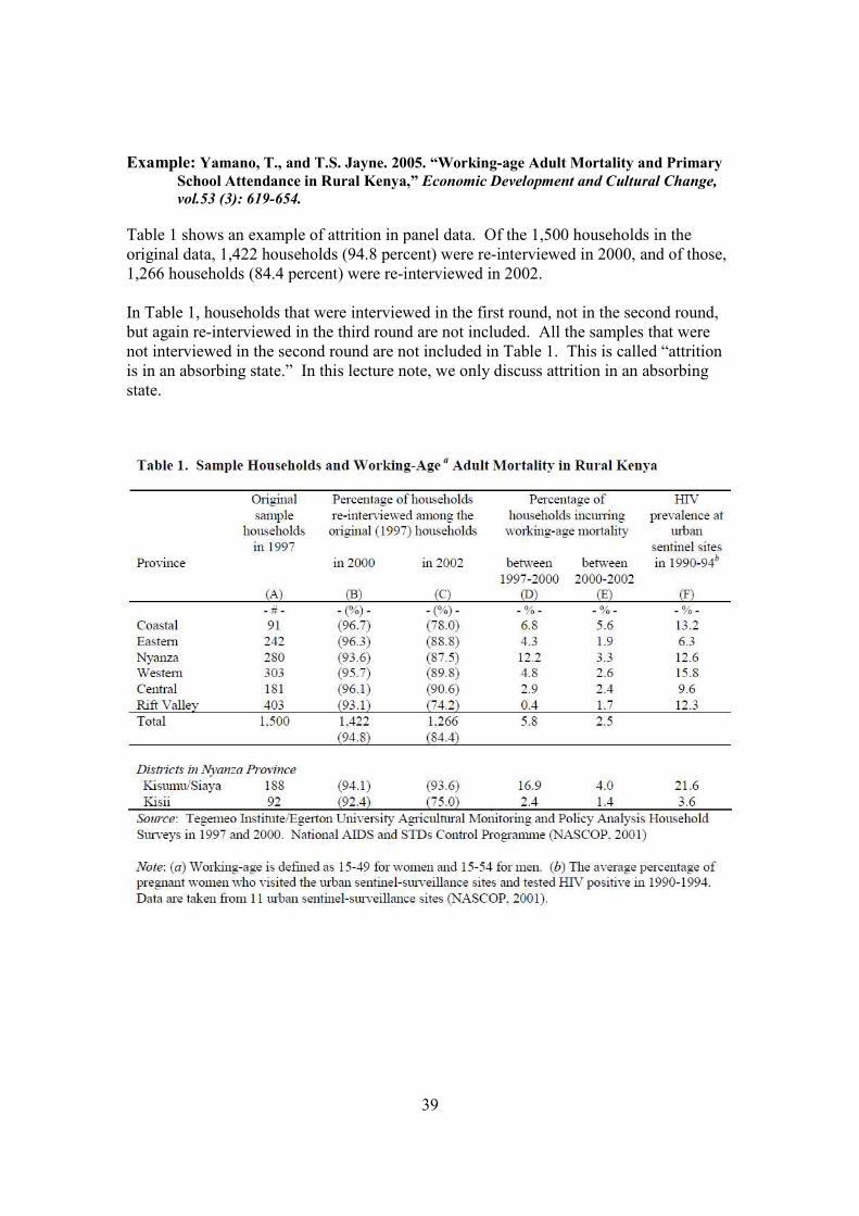
Example: Yamano, T., and T.S. Jayne. 2005. “Working-age Adult Mortality and Primary

School Attendance in Rural Kenya,” Economic Development and Cultural Change,

vol.53 (3): 619-654.

Table 1 shows an example of attrition in panel data. Of the 1,500 households in the

original data, 1,422 households (94.8 percent) were re-interviewed in 2000, and of those,

1,266 households (84.4 percent) were re-interviewed in 2002.

In Table 1, households that were interviewed in the first round, not in the second round,

but again re-interviewed in the third round are not included. All the samples that were

not interviewed in the second round are not included in Table 1. This is called “attrition

is in an absorbing state.” In this lecture note, we only discuss attrition in an absorbing

state.

40

41

42

Lecture 14: Propensity Score Matching

Propensity Score Matching Method

When we studied program evaluations previously, we define the probability of being in

the treatment group as:

)|1()( xwPxp == .

This is called the propensity score. For simple analyses, the propensity score can be used

to obtain the average treatment effect by calculating

∑=

− −−=N

i

iiiiiii xpxpyxpwNATE1

1 ))](ˆ1)((ˆ/[))(ˆ(

−−= ∑ ∑

= =

−Treatment

i

Control

i

iiiiii xpyxpyN1 1

1 ))(ˆ1/()(ˆ/

Or we can simply estimate a regression model:

iiii uxpwy +++= )(ˆ10 ββδ

But it is not clear if this is any better than estimating a model

iiii uxwy +++= ββδ 0 .

where xi is a 1-by-k vector.

A more popular approach is to use the propensity score to obtain matching estimators.

The idea is to match two observations that have the same or a very similar propensity

score and measure the difference in the outcome:

)](|[)](,0|[)](,1|[ 0101 xpyyExpwyExpwyE −==−=

as defined before, y1 is the outcome when the sample has actually received benefits from

a program and y0 is the outcome when the sample has not received any benefits from the

program. w indicates who are in the treatment group. For the sake of counterfactual

discussions, the treatment group may not receive benefits from the program, i.e.,

)](,1|[ 0 xpwyE = .

The main assumption that one indicator, the propensity score, can control for everything

except the participation in the program. For instance, suppose that a very critical

component is missing in the propensity score estimation, then the propensity score with

missing component wound match two observations that should not be matched.

43

See examples in the class.

44

Lecture 15: Simultaneous Equations Models

Simultaneous Bias

Consider a two-equation structural model

y1 = α1 y2 + $1 z1 + u1 (1)

y2 = α2 y1 + $2 z2 + u2 (2)

These two-equations are examples of structural equations because both equations contain

an endogenous variable. Or we call a set of these equations as a simultaneous equations

model (SEM) because these two equations simultaneously determine both y1 and y2. y1

and y2 are called endogenous variables, and z1 and z2 are called exogenous variables.

Finally u1 and u2 are called structural errors.

Because we have two endogenous variables and two equations, we can solve for each

endogenous variable in terms of exogenous variables and structural errors:

y2 = α2 (α1 y2 + $1 z1 + u1) + $2 z2 + u2

y2 = α2 α1 y2 + α2 $1 z1 +α2 u1 + $2 z2 + u2

(1-α2 α1)y2 = α2 $1 z1 + $2 z2 + α2 u1 + u2

Assuming that α2 α1≠1, we have

y2 = (α2 $1 /(1-α2 α1)) z1 + ($2 /(1-α2 α1)) z2 + (α2 u1+ u2 )/(1-α2 α1) y2 = δ1 z1 + δ2 z2 + v (3)

Thus, in (3), y2 is expressed in terms of exogenous variables. This is called a reduced

form equation, which has only exogenous variables and error terms, for y2. From (13-3),

we can show

Cov (y2, u1) = Cov (δ1 z1 + δ2 z2 + (α2 u1+ u2 )/(1-α2 α1), u1)

= )1

(12

2

12

ααα−

uE

= 2

1

12

2

1uσαα

α−

This is not zero if α2 α1≠1 and α2 ≠ 0. Thus, in equation (13-1), y2 is correlated with the

error term, u1, and the estimated coefficient of y2 will be biased. This is called a

simultaneous bias. In equation (13-2), the estimated coefficient of y1 will be biased

because of the simultaneous bias.

45

Identification

Consider a two-equation model:

Supply curve: q = α1 p + $1 z + u1

Demand curve: q = α2 p + u2

In these simple equations, we have one exogenous variable in the supply curve, z. The

supply curve shifts up and down as z changes. Thus, we may call it as a supply-curve

shifter.

The demand curve does not have any demand-curve shifters, thus the demand curve does

not move. Therefore, when we find changes in price and quantity, we can assume that

the changes are caused by z and that the observed points (A, B, C) are on the demand

curve. Thus, by connecting these points, we can identify the demand curve.

In the previous lecture note, we have studied that we need at least one instrument to

identify one endogenous variable. In the demand equation, the endogenous variable is

the price, p, and the instrument is the supply-curve shifter, z. Thus, the price in the

demand curve equation is identified.

In contrast, we can not identify the supply curve because we do not have any instrument

to identify price in the supply equation.

Suppose now that we have these demand and supply curves. The only difference is that z

is included in the both equations:

Supply curve: q = α1 p + $ 1z + u1

Demand curve: q = α2 p + $ 2z + u2

A

B

C

A

C

Panel 1 Panel 2

Demand Curve Supply Curve

46

In this case, we can not identify either curve, because z is included in the both equations.

Thus, z does not satisfy the exclusion restrictions. This is illustrated in Panel 2. We

observe changes in price and quantity from A to C. But, because both curves can shift

from A to C, we can not trace curves. Both curves in Panel 2 could be steeper or flatter.

Reduced Form Equations in General Cases

In general, we can have more than two simultaneous equations (more than two

endogenous variables) at once. Suppose there are 3-endogenous variables:

y1 = f1(y2, y3, z1,z2, z3, z4)

y2 = f2(y1, y3, z1, z2, z5, z6, z7)

y3 = f3(y1, y2, z1, z2, z8, z9, z10)

The reduced form equation for each endogenous variable will contain all of the

exogenous variables:

y1 = f1(z1,z2, z3, z4, z5, z6, z7, z8, z9, z10)

y2 = f2(z1,z2, z3, z4, z5, z6, z7, z8, z9, z10)

y3 = f3(z1,z2, z3, z4, z5, z6, z7, z8, z9, z10)

From these reduced form equations, we can identify endogenous variables in the

structural from equations.

Example 15-1: Inflation and Openness by using Openness.dta

See Example 16.4 and 16.6 in Wooldridge:

The Reduced Form Equation for “Open” . reg open lpcinc lland Source | SS df MS Number of obs = 114 -------------+------------------------------ F( 2, 111) = 45.17 Model | 28606.1936 2 14303.0968 Prob > F = 0.0000 Residual | 35151.7966 111 316.682852 R-squared = 0.4487 -------------+------------------------------ Adj R-squared = 0.4387 Total | 63757.9902 113 564.230002 Root MSE = 17.796 ------------------------------------------------------------------------------ open | Coef. Std. Err. t P>|t| [95% Conf. Interval] -------------+---------------------------------------------------------------- lpcinc | .5464812 1.49324 0.37 0.715 -2.412473 3.505435 lland | -7.567103 .8142162 -9.29 0.000 -9.180527 -5.953679 _cons | 117.0845 15.8483 7.39 0.000 85.68006 148.489 ------------------------------------------------------------------------------

The OLS for inflation . reg inf open lpcinc Source | SS df MS Number of obs = 114 -------------+------------------------------ F( 2, 111) = 2.63 Model | 2945.92812 2 1472.96406 Prob > F = 0.0764

47

Residual | 62127.4936 111 559.70715 R-squared = 0.0453 -------------+------------------------------ Adj R-squared = 0.0281 Total | 65073.4217 113 575.870989 Root MSE = 23.658 ------------------------------------------------------------------------------ inf | Coef. Std. Err. t P>|t| [95% Conf. Interval] -------------+---------------------------------------------------------------- open | -.2150695 .0946289 -2.27 0.025 -.402583 -.027556 lpcinc | .0175683 1.975267 0.01 0.993 -3.896555 3.931692 _cons | 25.10403 15.20522 1.65 0.102 -5.026122 55.23419 ------------------------------------------------------------------------------

The 2SLS for inflation . ivreg inf (open= lland) lpcinc Instrumental variables (2SLS) regression Source | SS df MS Number of obs = 114 -------------+------------------------------ F( 2, 111) = 2.79 Model | 2009.22775 2 1004.61387 Prob > F = 0.0657 Residual | 63064.194 111 568.145892 R-squared = 0.0309 -------------+------------------------------ Adj R-squared = 0.0134 Total | 65073.4217 113 575.870989 Root MSE = 23.836 ------------------------------------------------------------------------------ inf | Coef. Std. Err. t P>|t| [95% Conf. Interval] -------------+---------------------------------------------------------------- open | -.3374871 .1441212 -2.34 0.021 -.6230728 -.0519014 lpcinc | .3758247 2.015081 0.19 0.852 -3.617192 4.368841 _cons | 26.89934 15.4012 1.75 0.083 -3.619161 57.41783 ------------------------------------------------------------------------------ Instrumented: open Instruments: lpcinc lland ------------------------------------------------------------------------------

The estimated coefficient changes from -0.215 to -0.337. There is no over-identification problem because the number of endogenous variable and the instrument is both one.

48

Lecture 16: Systems of Equations (SUR, GMM, and 3SLS)

Seemingly Unrelated Regression (SUR) Model

Consider a set of G linear equations:

y1 = X1 $1 + ɛ1

y2 = X2 $2 + ɛ 2 (1)

…

yG = XG $G + ɛ G

where Xg is a N-by-kg matrix (kg may differ across equations but often not in

applications). (g = 1, 2, …, G) yg, $2, ɛ 2 are all N-by-1 vectors. Xg contains only

exogenous variables.

The system (1) is called “Seemingly Uncorrelated” because each equation seems

unrelated with other equations. However, it is often assumed that error terms are

correlated across equations. For example, many applications estimated a set of demand

functions for families. In this case, error terms are most likely to be correlated across

equations.

The system (1) can be written as

+

=

GGGG X

X

X

y

y

y

ε

ε

ε

β

β

β

2

1

2

1

2

1

2

1

...00

0...0

0...0

(2)

NG x 1 NG x K K x 1 NG x 1

Where K is a sum of kg for g = 1, …, G.

The error term has the following properties:

ɛɛɛɛ = [ɛɛɛɛ'1, ɛɛɛɛ'2, …, ɛɛɛɛ'G]'

E[ɛɛɛɛ | X1, X2, …, XG] = 0

E[ɛɛɛɛɛɛɛɛ' | X1, X2, …, XG] = ΩΩΩΩ

ɛɛɛɛ is a NG-by-1 vector, and E[ɛɛɛɛɛɛɛɛ'] = V is a NG-by-NG matrix. We further assume that

E[ɛit ɛjs | X1, X2, …, XG] = σij if t = s and 0 otherwise.

For instance, this indicates that the error term for the demand for pork (i-th equation) at

time t, ɛit, is correlated with the error term for the demand for chicken (j-th equation) at

time t, ɛjt. But the error terms are uncorrelated across time.

49

For one equation, the variance-covariance matrix of ɛɛɛɛi is

E[ɛɛɛɛi ɛɛɛɛi'| X1, X2, …, XG] = σii IN

The variance-covariance matrix of ɛɛɛɛi and ɛɛɛɛj is

E[ɛɛɛɛi ɛɛɛɛj'| X1, X2, …, XG] = σij IN

Thus, for all the observations

=Ω=′

III

III

III

XXXE

GGGsG

G

G

G

σσσ

σσσ

σσσ

εε

...

...

...

],...,,|[

1

22221

11211

21 (3)

(What is the order of this square matrix?)

From (2), we have

εβ

ε

ε

ε

β

β

β

+=

+

=

X

X

X

X

y

y

y

GGGG

2

1

2

1

2

1

2

1

...00

0...0

0...0

(4)

Thus, the error term of the SUR model in (4) has a variance-covariance of (3). Thus, a

GLS estimation can be applied to the SUR model. Define

=Σ

GGGG

G

G

σσσ

σσσ

σσσ

...

...

...

21

22221

11211

so, in (3),

NGGNNGNG IandI ⊗Σ=Ω⊗Σ=Ω −− 11

Denoting the i j th element of 1−ΣG by ijσ , thus

50

=Σ−

GGGG

G

G

G

σσσ

σσσ

σσσ

...

...

...

21

22221

11211

1 .

The GLS estimator is

yIXXIXyXXX NGNGSURGLS )(])([][ˆ 111111 ⊗Σ′⊗Σ′=Ω′Ω′= −−−−−−−β .

See Greene pp342 for more details.

Some important results on the SUR Model:

SUR1 If the equations are actually unrelated, then there is no payoff to GLS

estimation.

SUR2 If the same set of independent variables are used for each equation,

X1=X2= … =XG, then GLS and OLS are identical.

SUR3 If the independent variables on one block of equations are a subset of

those in another, then GLS brings on efficiency gain over OLS in

estimation of the smaller set of equations.

We will examine these results in examples.

Testing SUR2

Define

( ) )....,,,(),...,,,(),...,,,(,...,,, 21212121 GGGG XXXdiagXanduuuuyyyy =′′′=′′′=′′′= ββββ

Then, we can write (12-4) as

uXy += β

Then the GLS estimator is

yIXXIXyXXX NGNGGLS )())(()(ˆ 111111 ⊗Σ′⊗Σ′=Ω′Ω′= −−−−−−β (5)

Suppose all equations have the same set of independent variables, X1=X2= … =XG=X.

Then, we can write XIX G ⊗= and XIX G ⊗=′ . Thus,

yIXIXIIXI NGGGNGGGLS ))(()])()([(ˆ 111 ⊗Σ′⊗⊗⊗Σ′⊗= −−−β

yXXIX GGG )()])([( 111 ′⊗Σ⊗′⊗Σ= −−−

yXXX GG )()]([( 111 ′⊗Σ′⊗Σ= −−−

yXXX GG )]()([(11 ′⊗Σ′⊗Σ= −−

51

yXXXIG ])([( 1 ′′⊗= −

yXXX ′′= −1)(

′′

′′

′′

=

−

−

−

Gy

y

y

XXX

XXX

XXX

2

1

1

1

1

)(00

00)(0

000)(

=

′′

′′

′′

=

−

−

−

OLSG

OLS

OLS

GyXXX

yXXX

yXXX

,

,2

,1

1

2

1

1

1

ˆ

ˆ

ˆ

)(

)(

)(

β

β

β

(We have used a rule on Kronecker Product that )())(( BDACDCBA ⊗=⊗⊗ when AC

and BD can be defined. See Greene A.5.5. in Appendix A.) Thus, the GLS estimators

are identical to the OLS estimators.

Example 14-1: Wage and Fringe Benefits (FRINGE.dta)

In this example, we estimate a two-equation system for hourly wage and hourly benefits.

There are 616 workers in the data set. The FGLS results for a SUR model are presented

below.

FGL Estimation for a SUR Model . sureg (hrearn educ exper exper2 union) ( hrbens educ exper exper2 union), small dfk Seemingly unrelated regression ---------------------------------------------------------------------- Equation Obs Parms RMSE "R-sq" F-Stat P ---------------------------------------------------------------------- hrearn 616 4 4.460274 0.1552 28.06 0.0000 hrbens 616 4 .5593549 0.2971 64.56 0.0000 ---------------------------------------------------------------------- ------------------------------------------------------------------------------ | Coef. Std. Err. t P>|t| [95% Conf. Interval] -------------+---------------------------------------------------------------- hrearn | educ | .5069603 .0685878 7.39 0.000 .3723975 .6415231 exper | -.0131478 .05253 -0.25 0.802 -.1162067 .0899112 exper2 | .0030274 .0011343 2.67 0.008 .0008021 .0052527 union | 1.098166 .3965588 2.77 0.006 .3201539 1.876177 _cons | -1.728478 1.009515 -1.71 0.087 -3.709053 .2520974 -------------+---------------------------------------------------------------- hrbens | educ | .0790536 .0086015 9.19 0.000 .0621783 .0959288 exper | .0485195 .0065877 7.37 0.000 .0355951 .061444 exper2 | -.000781 .0001422 -5.49 0.000 -.0010601 -.0005019 union | .4901085 .0497317 9.86 0.000 .3925394 .5876775 _cons | -.7495522 .1266015 -5.92 0.000 -.9979326 -.5011719 ------------------------------------------------------------------------------

52

Here, we examine a correlation between residuals from two equations. The test indicates

that the residuals from the two equations are correlated with a correlation of 0.3377. The

Breush-Pagan test suggests that the two are correlated significantly. It is not surprising to

find a strong correlation because the same unobserved variables, such as ability, across

two equations should be correlated. Correlation matrix of residuals: hrearn hrbens hrearn 1.0000 hrbens 0.3377 1.0000 Breusch-Pagan test of independence: chi2(1) = 70.259, Pr = 0.0000

Now, we estimate the two equations separately by OLS. The results below are exactly

the same as in the FGLS-SUR model above. This confirms SUR2, GLS and OLS are

identical if the same set of independent variables is used in a SUR model. The model

above is not useless because we could at least test if the residuals from equations are

correlated.

OLS on Hourly Wage: . reg hrearn educ exper exper2 union Source | SS df MS Number of obs = 616 -------------+------------------------------ F( 4, 611) = 28.06 Model | 2232.63395 4 558.158487 Prob > F = 0.0000 Residual | 12155.2624 611 19.8940465 R-squared = 0.1552 -------------+------------------------------ Adj R-squared = 0.1496 Total | 14387.8963 615 23.3949534 Root MSE = 4.4603 ------------------------------------------------------------------------------ hrearn | Coef. Std. Err. t P>|t| [95% Conf. Interval] -------------+---------------------------------------------------------------- educ | .5069603 .0685878 7.39 0.000 .372264 .6416567 exper | -.0131478 .05253 -0.25 0.802 -.116309 .0900135 exper2 | .0030274 .0011343 2.67 0.008 .0007999 .0052549 union | 1.098166 .3965588 2.77 0.006 .3193819 1.876949 _cons | -1.728478 1.009515 -1.71 0.087 -3.711019 .2540629 ------------------------------------------------------------------------------

OLS on Hourly Benefits: . reg hrbens educ exper exper2 union Source | SS df MS Number of obs = 616 -------------+------------------------------ F( 4, 611) = 64.56 Model | 80.8036641 4 20.200916 Prob > F = 0.0000 Residual | 191.16841 611 .312877922 R-squared = 0.2971 -------------+------------------------------ Adj R-squared = 0.2925 Total | 271.972074 615 .442231015 Root MSE = .55935 ------------------------------------------------------------------------------ hrbens | Coef. Std. Err. t P>|t| [95% Conf. Interval] -------------+---------------------------------------------------------------- educ | .0790536 .0086015 9.19 0.000 .0621615 .0959456 exper | .0485195 .0065877 7.37 0.000 .0355823 .0614568 exper2 | -.000781 .0001422 -5.49 0.000 -.0010603 -.0005016 union | .4901085 .0497317 9.86 0.000 .3924426 .5877743 _cons | -.7495522 .1266015 -5.92 0.000 -.9981791 -.5009254 ------------------------------------------------------------------------------

To test SUR 3, we add two independent variables, married and male, to the first equation

but not in the second. Thus, the independent variables in the second equation are a subset

53

of the set of independent variables in the first equation. The results below confirms

SUR3, the results below on the second equation are identical to the OLS results. . sureg (hrearn educ exper exper2 union married male) ( hrbens educ exper exper2 union), small dfk corr Seemingly unrelated regression ---------------------------------------------------------------------- Equation Obs Parms RMSE "R-sq" F-Stat P ---------------------------------------------------------------------- hrearn 616 6 4.378737 0.1884 21.87 0.0000 hrbens 616 4 .5593549 0.2971 64.56 0.0000 ---------------------------------------------------------------------- ------------------------------------------------------------------------------ | Coef. Std. Err. t P>|t| [95% Conf. Interval] -------------+---------------------------------------------------------------- hrearn | educ | .4866347 .0674135 7.22 0.000 .3543755 .6188939 exper | -.0385265 .0525284 -0.73 0.463 -.1415826 .0645295 exper2 | .0032235 .0011205 2.88 0.004 .0010252 .0054218 union | .8654272 .3933037 2.20 0.028 .0938007 1.637054 married | .4591233 .3970173 1.16 0.248 -.3197891 1.238036 male | 1.212324 .3788968 3.20 0.001 .4689623 1.955685 _cons | -2.117965 .9962684 -2.13 0.034 -4.072554 -.1633757 -------------+---------------------------------------------------------------- hrbens | educ | .0790536 .0086015 9.19 0.000 .0621782 .0959289 exper | .0485195 .0065877 7.37 0.000 .0355951 .061444 exper2 | -.000781 .0001422 -5.49 0.000 -.0010601 -.0005019 union | .4901085 .0497317 9.86 0.000 .3925393 .5876776 _cons | -.7495522 .1266015 -5.92 0.000 -.997933 -.5011715 ------------------------------------------------------------------------------

End of Example 14-1

Generalized Method of Moments (GMM) Estimation

Suppose we have a set of equations and for observation i, we have

yi = Xi $ + ɛi

where yi is a G-by-1 vector (2-by-1 if there are two equations), Xi is a G-by-K matrix, and

ɛi is a G-by-1 error vector.

Assumption SIV 1: E(Z'i ui) = 0, where Zi is a G-by-L matrix of observable

instrumental variables.

Assumption SIV 2: rank (Z'i Xi) = K.

SIV stands for “system instrumental variables.” We also assume E(ui)=0.

The order condition, L ≥ K, should be satisfied when the rank condition (SIV 2) is met.

We have a set of equations with potentially endogenous variables:

y1 = X1 $1 + ɛ1

y2 = X2 $2 + ɛ 2 (6)

…

yG = XG $G + ɛ G

where we can also write

54

Y = X$$$$ + ɛɛɛɛ

Where Y is a NG-by-1 vector, X is a NG-by-K matrix, and ɛɛɛɛ is a NG-by-1 vector. Under

Assumptions SIV 1 and SIV 2, SIVβ is the unique K-by-1 vector solving the linear set

population moment conditions:

E[Z' (Y - X SIVβ )] = 0 (7)

Because sample averages are consistent estimators of population moments, the analogy

applied to condition (7) suggests choosing SIVβ to solve

∑=

− =−′N

i

SIViii XYZN1

1 0)ˆ( β (8)

Z is a NG-by-L matrix. When L = K,

SIVβ =(Z'X)-1Z'Y

This is called the system IV (SIV) estimator.

When L > K (so we have more columns in the IV matrix Z than we need for

identification), choosing SIVβ is more complicated. The equation (13-8) does not have a

solution. Instead, we choose SIVβ to make the vector in equation (13-8) as “small” as

possible in the sample. One idea is to minimize this:

−′

′

−′ ∑∑

==

N

i

SIViii

N

i

SIViii XYZXYZ11

)ˆ()ˆ( ββ

But, a more general class of estimators is obtained by using a weighting matrix in the

quadratic form. Let W be an L-by-L symmetric, positive semidefinite matrix. The

generalized method of moments (GMM) estimator that solves the problem

min

−′

′

−′ ∑∑

==

N

i

SIViii

N

i

SIViii XYZWXYZ11

)ˆ(ˆ)ˆ( ββ

or

[ ] [ ])ˆ(ˆ)ˆ(min SIVSIV XYZWXYZ βββ

−′′

−′

[ ][ ]SIVSIV XZWYZWZXZY βββ

ˆˆˆˆmin ′−′′′−′

SIVSIVSIVSIV XZWZXXZWZYYZWZXYZWZY βββββ

ˆˆˆˆˆˆˆˆmin ′′′+′′−′′′−′′

F.O.C. is

0ˆˆ2ˆˆ =′′+′′−′′− SIVXZWZXXZWZYYZWZX β

55

YZWZXXZWZX SIV′′=′′ ˆˆˆ β

YZWZXXZWZXGMM′′′′= − ˆ)ˆ(ˆ 1β (9)

Assumption SIV 3: whereNasWWp

,ˆ ∞→→ W is nonrandom, symmetric, L-by-L

positive definite matrix.

Theorem (Consistency of GMM): Under assumptions SIV 1-3, the GMM estimators are

consistent and asymptotically normally distributed.

The System 2SLS Estimator

Suppose we choose

1)/(ˆ −′= NZZW

which is a consistent estimator of [E( iiZZ ′ )]-1. Assumption SIV 3 simply requires that

E( iiZZ ′ ) exist and be nonsingular. When we plug this into equation (9), we get

YZZZZXXZZZZXSLSS′′′′′′= −−− 111

2 )())((β (10)

This is called the system 2SLS estimator.

The Optimal Weighting Matrix

The Procedure

1. Let iniβ~

be an initial consistent estimator of β. In most cases this is the system 2SLS

estimator.

2. Obtain the G-by-1 residual vectors

iniiii Xy βε~~ −= for i = 1, 2, …, N

3. A generally consistent estimator of Λ is ∑=

− ′′=ΛN

i

iiii ZZN1

1 ~~ˆ εε

4. Choose

1

1

11 ~~ˆˆ−

=

−−

′′=Λ= ∑N

i

iiii ZZNW εε

and use this matrix to obtain the asymptotically optimal GMM estimator.

The Three-Stage Least Squares (3SLS) Estimator

The 3SLS estimator is a GMM estimation that uses a particular weighting matrix. Let

SLSSiii Xyu 2

~~ β−= be the residual from an initial estimation (usually a system 2SLS), then

define

∑=

− ′=ΩN

i

iiuuN1

1 ~~

56

Using the same arguments as in the FGLS case, )~~(ˆii

P uuE=Ω→Ω . The weighting

matrix used by 3SLS is

1

1

1

1 ]/)ˆ([ˆˆ −

−

=

− Ω⊗′=

Ω′= ∑ NZIZZZNW N

N

i

ii

Plugging this into (9), we get

YZZIZZXXZZIZZX NNSLS′Ω⊗′′′Ω⊗′′= − )ˆ(])ˆ([ˆ 1

3β (11)

This is different from the traditional 3SLS estimator in most textbooks, such as Greene

(pp. 406 in 5e). The traditional 3SLS estimator is

YIXXIX NNSLST )ˆ(ˆ]ˆ)ˆ(ˆ[ˆ 111

3

−−− Ω⊗′Ω⊗′=β

where XZZZandZX ii′′=ΠΠ≡ −1)(ˆˆˆ . (Note that in Greene notations are different.)

In short, the GMM definition of 3SLS is more generally valid, and it reduces to the

standard definition in the traditional simulation equations setting.

57

Lecture 17: Single Equation GMM and STATA Programs

In Lecture Note 14, we have studied GMM estimations in term of systems of equations.

In this lecture note, we take a step back and study a single equation GMM.

Generalized Method of Moments (GMM) Estimation

Suppose we have an equation and for observation i, we have

yi = Xi $ + ɛi i = 1, …, N.

where Xi , which is a 1-by-K vector, may contain some endogenous variables that

potentially correlated with the error term. Further, suppose that we have instrumental

variables that are correlated with the endogenous variables but not with the error term.

We denote a matrix with instrumental variables and exogenous independent variables as

Zi, which is 1-by-L vector.

Thus, we can also write

Y = X$$$$ + ɛɛɛɛ, , , , E(Z'ɛɛɛɛ)=0

Where Y is a N-by-1 vector, X is a N-by-K matrix, Z is a N-by-L matrix, and ɛɛɛɛ is a N-by-

1 vector. Under usual assumptions on instrumental variables estimation, IVβ is the

unique K-by-1 vector solving the linear set population moment conditions:

E[Z' (Y - X IVβ )] = 0 (1)

Because sample averages are consistent estimators of population moments, the analogy

applied to condition (15-1) suggests choosing IVβ to solve

∑=

− =−′N

i

IViii XYZN1

1 0)ˆ( β (2)

When L = K,

SIVβ =(Z'X)-1Z'Y

As we know already, this is called the IV estimator, but this can be thought as a special

case of GMM estimators. The basic principle of the method of moments is to choose

the parameter estimate so that the corresponding sample moments, Equation (1) in this

case, are also equal to zero.

When L > K (so we have more columns in the IV matrix Z than we need for

identification), choosing GMMβ is more complicated. Instead, we choose GMMβ to make

58

the distance between the two vectors below as “small” as possible in the sample:

′−′∑=

N

i

GMMiiii XZYZ1

)ˆ( β

To measure the distance between the two vectors, we construct a quadratic form with a

weighting matrix. LetW be an L-by-L symmetric, positive semidefinite matrix. Thus,

the generalized method of moments (GMM) estimator solves the minimizing problem:

min

−′

′

−′ ∑∑

==

N

i

SIViii

N

i

SIViii XYZWXYZ11

)ˆ(ˆ)ˆ( ββ

or

[ ] [ ])ˆ(ˆ)ˆ(min SIVSIV XYZWXYZ βββ

−′′

−′

[ ][ ]SIVSIV XZWYZWZXZY βββ

ˆˆˆˆmin ′−′′′−′

SIVSIVSIVSIV XZWZXXZWZYYZWZXYZWZY βββββ

ˆˆˆˆˆˆˆˆmin ′′′+′′−′′′−′′

F.O.C. is

0ˆˆ2ˆˆ =′′+′′−′′− SIVXZWZXXZWZYYZWZX β

YZWZXXZWZX SIV′′=′′ ˆˆˆ β

YZWZXXZWZXGMM′′′′= − ˆ)ˆ(ˆ 1β (3)

The asymptotically consistent estimator of the variance of the GMM estimator is

11 )ˆ(ˆˆ)ˆ()ˆ( −− ′′′Λ′′′= XZWZXXZWWZXXZWZXV GMMβ (4)

where )()( 2

iiii ZVarZZE εε =′≡Λ .

As we will see below, GMM estimator becomes to various least square estimators

depending on how we choose Wand ˆΛ . First, we start with the optimal (i.e., the most

efficient) GMM estimator.

Efficient GMM Estimator

In (4), we recognize that the variance of the GMM estimator will have a least asymptotic

variance if we choose 1ˆ −Λ=W . Then, the least asymptotic variance of the GMM

estimator is

111111 )()()ˆ( −−−−−− ′Λ′′ΛΛΛ′′Λ′= XZZXXZZXXZZXV GMMβ

11111 )()( −−−−− ′Λ′′Λ′′Λ′= XZZXXZZXXZZX 11 )( −− ′Λ′= XZZX (5)

59

We can obtain a consistent estimator of )()( 2

iiii ZVarZZE εε =′≡Λ from )ˆ( 2

iii ZZE ′ε ,

where the residual is obtained from consistent estimators (but could be inefficient

estimators such as 2SLS estimators). Therefore, we can construct a procedure to obtain

the optimal weighting matrix as:

The Optimal Weighting Matrix

The Procedure

5. Let iniβ~

be an initial consistent estimator of β. In most cases this is the system 2SLS

estimator.

6. Obtain residuals: iniiii Xy βε~~ −= for i = 1, 2, …, N

7. A generally consistent estimator of Λ is ∑=

− ′=ΛN

i

iii ZZN1

21 ~ˆ ε

8. Choose

1

1

211ˆˆ−

=

−−

′=Λ= ∑N

i

iii ZZNW ε

and use this weighting matrix to obtain the asymptotically optimal GMM estimator.

(See Examples below)

The GMM=2SLS Estimator

Up to this point, we have not made a homoskedasticity assumption. But, what happens if

we do? Under a conditional homoskedasticity, we have

22 )|( σε =ii XE .

Then,

)()( 22

iiiii ZZEZZE ′=′≡Λ σε .

A consistent estimator of Λ is ZZ ′=Λ 2ˆˆ σ . By following the general rule to obtain the

least variance, we choose the weighting matrix as

1121 )()ˆ(ˆˆ −−− ′=Λ= ZZW σ .

When we plug this into equations (4) and (5), we get

YZZZZXXZZZZXSLS′′′′′′= −−− 111

2 )())((β (6)

11 ))(()ˆ( −− ′′′= XZZZZXV GMMβ (7)

This is the 2SLS estimator and its variance.

STATA Programs on OLS, robust-OLS, IV, and GMM.

Example 15-1: A STATA Program of OLS on CARD.dta . #delimit;

60

delimiter now ; . set more off; . set matsize 800; . clear; . use c:\docs\fasid\classes\econometrics\wooldridge_data\card.dta; . ** A matrix with everything; . mat accum x=lwage educ exper expersq black smsa south; (obs=3010) . ** YY; . matrix yy=x[1,1]; . ** XY; . matrix xy=x[2...,1]; . ** XX; . matrix xx=x[2...,2...]; . ** Obtain b; . matrix b=(syminv(xx)*xy)'; . ** Obtain SSR; . matri s=(yy-2*b*xy+b*xx*b')/(3010-7); . mat list s; symmetric s[1,1] lwage lwage .14001865 . ** Obtain variances; . matrix v=s*syminv(xx); . ereturn post b v; . ereturn display; ------------------------------------------------------------------------------ | Coef. Std. Err. z P>|z| [95% Conf. Interval] -------------+---------------------------------------------------------------- educ | .074009 .0035054 21.11 0.000 .0671385 .0808795 exper | .0835958 .0066478 12.57 0.000 .0705664 .0966253 expersq | -.0022409 .0003178 -7.05 0.000 -.0028638 -.0016179 black | -.1896315 .0176266 -10.76 0.000 -.224179 -.1550841 smsa | .161423 .0155733 10.37 0.000 .1308999 .191946 south | -.1248615 .0151182 -8.26 0.000 -.1544927 -.0952303 _cons | 4.733664 .0676026 70.02 0.000 4.601166 4.866163 ------------------------------------------------------------------------------ . reg lwage educ exper expersq black smsa south; Source | SS df MS Number of obs = 3010 -------------+------------------------------ F( 6, 3003) = 204.93 Model | 172.165628 6 28.6942714 Prob > F = 0.0000 Residual | 420.476016 3003 .140018653 R-squared = 0.2905 -------------+------------------------------ Adj R-squared = 0.2891 Total | 592.641645 3009 .196956346 Root MSE = .37419 ------------------------------------------------------------------------------ lwage | Coef. Std. Err. t P>|t| [95% Conf. Interval]

61

-------------+---------------------------------------------------------------- educ | .074009 .0035054 21.11 0.000 .0671357 .0808823 exper | .0835958 .0066478 12.57 0.000 .0705612 .0966305 expersq | -.0022409 .0003178 -7.05 0.000 -.0028641 -.0016177 black | -.1896315 .0176266 -10.76 0.000 -.2241929 -.1550702 smsa | .161423 .0155733 10.37 0.000 .1308876 .1919583 south | -.1248615 .0151182 -8.26 0.000 -.1545046 -.0952184 _cons | 4.733664 .0676026 70.02 0.000 4.601112 4.866216 ------------------------------------------------------------------------------

Example 15-2: A STATA Program of robust-OLS on CARD.dta . #delimit; delimiter now ; . set more off; . set matsize 800; . clear; . use c:\docs\fasid\classes\econometrics\wooldridge_data\card.dta; . reg lwage educ exper expersq black smsa south; Source | SS df MS Number of obs = 3010 -------------+------------------------------ F( 6, 3003) = 204.93 Model | 172.165628 6 28.6942714 Prob > F = 0.0000 Residual | 420.476016 3003 .140018653 R-squared = 0.2905 -------------+------------------------------ Adj R-squared = 0.2891 Total | 592.641645 3009 .196956346 Root MSE = .37419 ------------------------------------------------------------------------------ lwage | Coef. Std. Err. t P>|t| [95% Conf. Interval] -------------+---------------------------------------------------------------- educ | .074009 .0035054 21.11 0.000 .0671357 .0808823 exper | .0835958 .0066478 12.57 0.000 .0705612 .0966305 expersq | -.0022409 .0003178 -7.05 0.000 -.0028641 -.0016177 black | -.1896315 .0176266 -10.76 0.000 -.2241929 -.1550702 smsa | .161423 .0155733 10.37 0.000 .1308876 .1919583 south | -.1248615 .0151182 -8.26 0.000 -.1545046 -.0952184 _cons | 4.733664 .0676026 70.02 0.000 4.601112 4.866216 ------------------------------------------------------------------------------ . predict rhat, residuals; . ** creating rx variables; . gen reduc=rhat*educ; . gen rexper=rhat*exper; . gen rexpersq=rhat*expersq; . gen rblack=rhat*black; . gen rsmsa=rhat*smsa; . gen rsouth=rhat*south; . ** A matrix with everything; . gen one=1; . mat accum x=lwage educ exper expersq black smsa south one, noc;

62

(obs=3010) . mat accum xrrx=reduc rexper rexpersq rblack rsmsa rsouth rhat, noc; (obs=3010) . ** YY; . matrix yy=x[1,1]; . ** XY; . matrix xy=x[2...,1]; . ** XX; . matrix xx=x[2...,2...]; . ** Obtain b; . matrix b=(syminv(xx)*xy)'; . ** Obtain variances; . matrix v=syminv(xx)*xrrx*syminv(xx); . ereturn post b v; . ereturn display; ------------------------------------------------------------------------------ | Coef. Std. Err. z P>|z| [95% Conf. Interval] -------------+---------------------------------------------------------------- educ | .074009 .0036378 20.34 0.000 .066879 .0811389 exper | .0835958 .0067248 12.43 0.000 .0704155 .0967762 expersq | -.0022409 .0003177 -7.05 0.000 -.0028637 -.0016181 black | -.1896315 .0174122 -10.89 0.000 -.2237587 -.1555043 smsa | .161423 .0151574 10.65 0.000 .1317149 .191131 south | -.1248615 .0153329 -8.14 0.000 -.1549134 -.0948096 one | 4.733664 .070076 67.55 0.000 4.596318 4.871011 ------------------------------------------------------------------------------ . reg lwage educ exper expersq black smsa south, robust; Regression with robust standard errors Number of obs = 3010 F( 6, 3003) = 217.74 Prob > F = 0.0000 R-squared = 0.2905 Root MSE = .37419 ------------------------------------------------------------------------------ | Robust lwage | Coef. Std. Err. t P>|t| [95% Conf. Interval] -------------+---------------------------------------------------------------- educ | .074009 .003642 20.32 0.000 .0668679 .0811501 exper | .0835958 .0067326 12.42 0.000 .0703948 .0967969 expersq | -.0022409 .0003181 -7.04 0.000 -.0028646 -.0016171 black | -.1896315 .0174324 -10.88 0.000 -.2238123 -.1554508 smsa | .161423 .0151751 10.64 0.000 .1316683 .1911776 south | -.1248615 .0153508 -8.13 0.000 -.1549606 -.0947625 _cons | 4.733664 .0701577 67.47 0.000 4.596102 4.871226 ------------------------------------------------------------------------------

Example 15-3: A STATA Program of IV on CARD.dta . #delimit; delimiter now ; . set more off;

63

. set matsize 800; . clear; . use c:\docs\fasid\classes\econometrics\wooldridge_data\card.dta; . ** A matrix with everything; . mat accum x=lwage educ nearc4 nearc2 exper expersq black smsa south; (obs=3010) . mat accum y=lwage educ exper expersq black smsa south; (obs=3010) . ** YY; . matrix yy=x[1,1]; . ** ZY; . matrix zy=x[3...,1]; . ** ZZ; . matrix zz=x[3...,3...]; . ** XZ; . matrix xz1=x[2,3...]; . matrix xz2=x[5...,3...]; . matrix xz=xz1\xz2; . ** XX; . matrix xx=y[2...,2...]; . ** XY; . matrix xy=y[2...,1]; . ** Obtain b; . matrix b=(syminv(xz*syminv(zz)*xz')*xz*syminv(zz)*zy)'; . ** Obtain SSR; . matri s=(yy-2*b*xy+b*xx*b')/(3010-7); . mat list s; symmetric s[1,1] lwage lwage .16863299 . ** Obtain variances; . matrix v=s*syminv(xz*syminv(zz)*xz'); . ereturn post b v; . ereturn display; ------------------------------------------------------------------------------ | Coef. Std. Err. z P>|z| [95% Conf. Interval] -------------+---------------------------------------------------------------- educ | .1608487 .0486291 3.31 0.001 .0655375 .25616 exper | .1192112 .0211779 5.63 0.000 .0777033 .1607191 expersq | -.0023052 .0003507 -6.57 0.000 -.0029925 -.001618 black | -.1019726 .0526187 -1.94 0.053 -.2051033 .0011582 smsa | .1165736 .0303135 3.85 0.000 .0571602 .175987 south | -.0951187 .0234721 -4.05 0.000 -.1411233 -.0491141 _cons | 3.272102 .8192563 3.99 0.000 1.666389 4.877815

64

------------------------------------------------------------------------------ . ivreg lwage (educ=nearc4 nearc2) exper expersq black smsa south; Instrumental variables (2SLS) regression Source | SS df MS Number of obs = 3010 -------------+------------------------------ F( 6, 3003) = 110.30 Model | 86.2367703 6 14.3727951 Prob > F = 0.0000 Residual | 506.404874 3003 .168632992 R-squared = 0.1455 -------------+------------------------------ Adj R-squared = 0.1438 Total | 592.641645 3009 .196956346 Root MSE = .41065 ------------------------------------------------------------------------------ lwage | Coef. Std. Err. t P>|t| [95% Conf. Interval] -------------+---------------------------------------------------------------- educ | .1608487 .0486291 3.31 0.001 .065499 .2561984 exper | .1192112 .0211779 5.63 0.000 .0776866 .1607358 expersq | -.0023052 .0003507 -6.57 0.000 -.0029928 -.0016177 black | -.1019726 .0526187 -1.94 0.053 -.2051449 .0011997 smsa | .1165736 .0303135 3.85 0.000 .0571363 .1760109 south | -.0951187 .0234721 -4.05 0.000 -.1411418 -.0490956 _cons | 3.272102 .8192563 3.99 0.000 1.665742 4.878462 ------------------------------------------------------------------------------ Instrumented: educ Instruments: exper expersq black smsa south nearc4 nearc2

Example 15-4: A STATA Program of GMM on CARD.dta . #delimit; delimiter now ; . set more off; . set matsize 800; . clear; . use c:\docs\fasid\classes\econometrics\wooldridge_data\card.dta; . ivreg lwage (educ=nearc4 nearc2) exper expersq black smsa south; Instrumental variables (2SLS) regression Source | SS df MS Number of obs = 3010 -------------+------------------------------ F( 6, 3003) = 110.30 Model | 86.2367703 6 14.3727951 Prob > F = 0.0000 Residual | 506.404874 3003 .168632992 R-squared = 0.1455 -------------+------------------------------ Adj R-squared = 0.1438 Total | 592.641645 3009 .196956346 Root MSE = .41065 ------------------------------------------------------------------------------ lwage | Coef. Std. Err. t P>|t| [95% Conf. Interval] -------------+---------------------------------------------------------------- educ | .1608487 .0486291 3.31 0.001 .065499 .2561984 exper | .1192112 .0211779 5.63 0.000 .0776866 .1607358 expersq | -.0023052 .0003507 -6.57 0.000 -.0029928 -.0016177 black | -.1019726 .0526187 -1.94 0.053 -.2051449 .0011997 smsa | .1165736 .0303135 3.85 0.000 .0571363 .1760109 south | -.0951187 .0234721 -4.05 0.000 -.1411418 -.0490956 _cons | 3.272102 .8192563 3.99 0.000 1.665742 4.878462 ------------------------------------------------------------------------------ Instrumented: educ

65

Instruments: exper expersq black smsa south nearc4 nearc2 ------------------------------------------------------------------------------ . predict rhat, residual; . ** Create Variables multiplied by rhat; . gen Znearc4=nearc4*rhat; . gen Znearc2=nearc2*rhat; . gen Zexper=exper*rhat; . gen Zexpersq=expersq*rhat; . gen Zblack=black*rhat; . gen Zsmsa=smsa*rhat; . gen Zsouth=south*rhat; . ** Create S-hat matrix; . mat accum ZrrZ=Znearc4 Znearc2 Zexper Zexpersq Zblack Zsmsa Zsouth rhat, noc; (obs=3010) . ** A matrix with y; . gen one=1; . mat accum x=lwage educ nearc4 nearc2 exper expersq black smsa south one, noc; (obs=3010) . mat accum y=lwage educ exper expersq black smsa south one, noc; (obs=3010) . ** YY; . matrix yy=x[1,1]; . ** ZY; . matrix zy=x[3...,1]; . ** ZZ; . matrix zz=x[3...,3...]; . ** XZ; . matrix xz1=x[2,3...]; . matrix xz2=x[5...,3...]; . matrix xz=xz1\xz2; . ** XX; . matrix xx=y[2...,2...]; . ** XY; . matrix xy=y[2...,1]; . ** Obtain GMMb; . matrix b=(syminv(xz*syminv(ZrrZ)*xz')*xz*syminv(ZrrZ)*zy)'; . ** Obtain variances; . matrix v=syminv(xz*syminv(ZrrZ)*xz'); . ereturn post b v;

66

. ereturn display; ------------------------------------------------------------------------------ | Coef. Std. Err. z P>|z| [95% Conf. Interval] -------------+---------------------------------------------------------------- educ | .1588387 .0484983 3.28 0.001 .0637838 .2538935 exper | .1182042 .0212941 5.55 0.000 .0764684 .1599399 expersq | -.0022962 .0003686 -6.23 0.000 -.0030186 -.0015738 black | -.1056934 .0519689 -2.03 0.042 -.2075506 -.0038361 smsa | .1170294 .0302564 3.87 0.000 .0577281 .1763308 south | -.096091 .0233983 -4.11 0.000 -.1419508 -.0502311 one | 3.307021 .8165958 4.05 0.000 1.706523 4.907519 ------------------------------------------------------------------------------ . ivgmm0 lwage (educ=nearc4 nearc2) exper expersq black smsa south; Instrumental Variables Estimation via GMM Number of obs = 3010 Root MSE = 0.4086 Hansen J = 2.6532 Chi-sq( 1) P-val = 0.10334 ------------------------------------------------------------------------------ | GMM lwage | Coef. Std. Err. z P>|z| [95% Conf. Interval] -------------+---------------------------------------------------------------- educ | .1588387 .0484983 3.28 0.001 .0637838 .2538935 exper | .1182042 .0212941 5.55 0.000 .0764684 .1599399 expersq | -.0022962 .0003686 -6.23 0.000 -.0030186 -.0015738 black | -.1056934 .0519689 -2.03 0.042 -.2075506 -.0038361 smsa | .1170294 .0302564 3.87 0.000 .0577281 .1763308 south | -.096091 .0233983 -4.11 0.000 -.1419508 -.0502311 _cons | 3.307021 .8165958 4.05 0.000 1.706523 4.907519 ------------------------------------------------------------------------------ Instrumented: educ Instruments: exper expersq black smsa south nearc4 nearc2 ------------------------------------------------------------------------------