lecture 8 feynman diagramms - atlas home...

1

Lecture 8Lecture 8Feynman diagrammsFeynman diagramms

SS2011SS2011: : ‚‚Introduction to Nuclear and Particle Physics, Part 2Introduction to Nuclear and Particle Physics, Part 2‘‘

2

Photon propagatorPhoton propagator

(1)

Electron-proton scattering by an exchange of virtual photons (‚Dirac-photons‘)

(2)

The photon vector field Aμ follows the wave equation:

where Jμ is the proton 4-current and

(3)

Solve the inhomogenuous wave equation (2) using the Green function:

The inhomogenuous solution of equation (2) can be written as

(4)

(5)

in Lorentz gauge.

Indeed, using (4) and (3) one obtaines eq. (2) again:

e-

e-

p

pvirtual photon

3


(6)

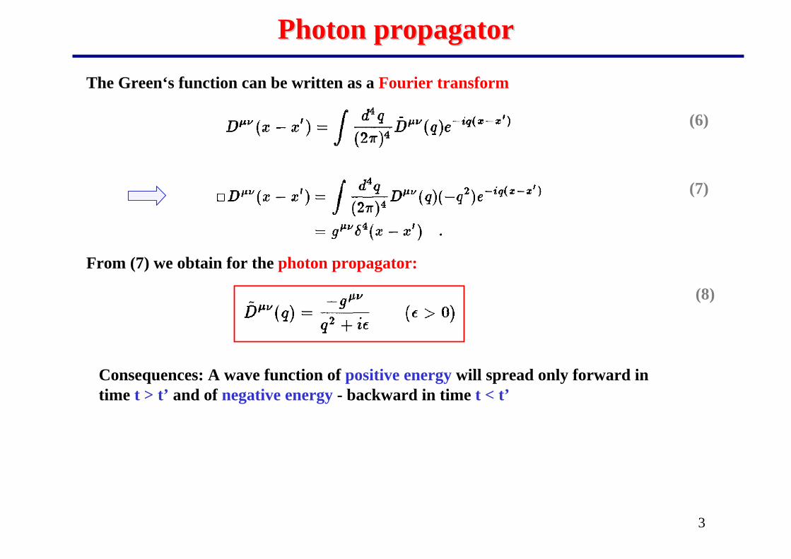
The Green‘s function can be written as a Fourier transform

(7)

From (7) we obtain for the photon propagator:

(8)

Consequences: A wave function of positive energy will spread only forward in time t > t’ and of negative energy - backward in time t < t’

4


(9)

The proton charge 4-current Jμ can be written as:

where ψi and ψf are the spinors of the proton in the initial and final states:

(10)

(11)From (10) and (9) we get

substitute (8) into (4)

(12)

(13)

The photon vector field Aμ:

0uu γ+≡

5

Feynmann diagrammsFeynmann diagramms

(14)For the free electron:

(15)

(16)

electron virtual photon proton

The matrix element (16) can be presented as a Feynman diagramm:

S-matrix element

6


For the electron:

For the photon:

For the incoming and outgoing photon we have:

7


Electron propagator:

S-matrix element:

Electron current :

Proton current:

8


emission absorption of photon

absorption emissionof virtual photon

1) Scattering of charged particles

2) Compton scattering emission of real photon

virtual electron

absorption of real photon

emission of real photon

virtual electron

absorption of real photon

9


3) Bremsstrahlung emission of real photon

virtual electron

Zeabsorption of virtual photon

virtual photon (time-like)

4) Pair creation and annihilation

10

Scattering of electrons on an external potentialScattering of electrons on an external potential

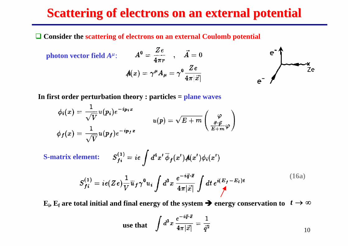
Consider the scattering of electrons on an external Coulomb potential

In first order perturbation theory : particles = plane waves

photon vector field Aμ :

S-matrix element:

use that

(16a)

Ei, Ef are total initial and final energy of the system energy conservation to ∞→t

11

Scattering of electrons on an external potentialScattering of electrons on an external potential

S-matrix element is

(17)

(18)

(19)

• Potential acts during the time period T (i.e. T is the interaction time) : -T/2 < t < T/2

Off-shell function f(ω): maximum at ω=0 (Ef=Ei), the amplitude ~T2; width ~1/T

matrix element

During the time -T/2 < t < T/2 the system can be in a state within the energy interval Ef , Ef+δE f

ρ(Ef )δE f – number of energy levels in this intervalρ(Ef ) – level density = number of states per energy interval

12

Feynmann diagramms:Feynmann diagramms: scattering of electrons scattering of electrons

(20)

(21)

Uncertainty relation:

If t >>T, f(ω) δ-function

(22)

Thus, transition probability W is obtained by an integration of dW over dE f :

Differential transition probability dW is

13

Feynmann diagramms:Feynmann diagramms: scattering of electronsscattering of electrons

For t >>T, f(ω) δ-function

(22)

(23)

Gold rule from Fermi:

w is the transition probability per unit time: w=W/T

Total cross section:= transition probability per unit time over jein - initial current:

(24)

14

Feynmann diagramms:Feynmann diagramms: scattering of electronsscattering of electronsThe scattering probability (17) is then

(25)

(26)

(27)

Furthermore, perfom the integration over the phase space:i.e. over the number of levels in the energy interval Ef , Ef+δE f and the direction of the particle in the solid angle element dΩf

Use that

factor 1/2Ef due to the normalization of 2Ef particles per volume V

)(2T ωπδ⇒∞→

S-matrix element

15

Feynmann diagramms: Feynmann diagramms: scattering of electronsscattering of electrons

Then, the differential transition probability is

matrix element

(28)

(29)Initial current:

Differential cross section:

Using the explicit form for the matrix element (17), we obtain:

(30)

(31)

where since

16

Feynmann diagramms: nonFeynmann diagramms: non--relativistic caserelativistic case

Consider the non-relativistic limit:

(32)

(33)

From (31) Rutherford formula

17

Feynmann diagramms: relativistic caseFeynmann diagramms: relativistic case

Consider the scattering of relativistic electrons

For fermions: 1) avaraging over the spin of initial fermions

2) summation over the spin of the final fermions

∑iS2

1

∑fS

∑fi S,S2

1

Consider

Spin avaraging:

(34)

(35)

(36)

For different components α,β:(37)

8

Dirac spinors (cf. Lecture N 7)Dirac spinors (cf. Lecture N 7)

Free (anti-)fermions are fully defined by the spinors specified above (with normalization (L7.24)):

1) Spinors with positive energy (fermions):

2) Spinors with negative energy (anti-fermions):

Wave vector ψ : fermions

anti-fermions

spin ‚up‘ : spin ‚down‘

(L7.27)

(L7.26)

(L7.25)

19

Spinor tensorsSpinor tensors

(37)

Summing over spin gives:

0uu γ+≡Notation:

20


Summing over spins of the initial and final fermions – we may write in matrix form:

Notation: Spur=Sp=Tr

(38)

(39)

(40)

(41)

with

Result:

21


(42)where I is the 4x4 unitary matrix

2) Spur (even number of γμ) =0

Notation: a≡μμμ γγγγγ ==

+ 00Use that

Using (42), averaging over the spin of the initial fermions and summation over the spin of final fermions leads to:

(42)

(43)

mass of electron

22


Evaluate the scalar product in the cms of the process i+f:

(44)

(45)

Note: non-relativisticely:

(46)

Ep

≡β

Thus, substitute (45) in (31) :

eq. (46) describes the scattering of a relativistic spin ½ particle on a spin 0 target (e.g. nucleus) with large mass M !

23


For the high energy electrons, i.e. E>>m, β 1

we obtain the Mott cross section including the backscattering of the target of finite mass M:

eq. (47) describes the scattering of a relativistic spin ½ electron on a spin 0 target with large mass M (e.g. nuclei, pion)

(47)

lecture 8 feynman diagramms - atlas home...

Documents