lecture 7 lti discrete-time systems in the transform domaintania/teaching/dsp/lecture 7 lti...
TRANSCRIPT

LTI DiscreteLTI Discrete--Time SystemsTime Systems
in Transform Domainin Transform DomainSimple FiltersSimple Filters
Comb Filters Comb Filters (Optional reading)(Optional reading)
AllpassAllpass Transfer FunctionsTransfer Functions
Minimum/Maximum Phase Transfer FunctionsMinimum/Maximum Phase Transfer Functions
Complementary Filters Complementary Filters (Optional reading)(Optional reading)
Digital TwoDigital Two--Pairs Pairs (Optional reading)(Optional reading)
Tania Stathaki
811b

Simple Digital FiltersSimple Digital Filters
• Later in the course we shall review various
methods of designing frequency-selective
filters satisfying prescribed specifications
• We now describe several low-order FIR and
IIR digital filters with reasonable selective
frequency responses that often are
satisfactory in a number of applications

Simple FIR Digital FiltersSimple FIR Digital Filters
• FIR digital filters considered here have
integer-valued impulse response coefficients
• These filters are employed in a number of
practical applications, primarily because of
their simplicity, which makes them amenable
to inexpensive hardware implementations

Simple FIR Digital FiltersSimple FIR Digital Filters
Lowpass FIR Digital Filters
• The simplest lowpass FIR digital filter is the 2-
point moving-average filter given by
• The above transfer function has a zero at z = -1
and a pole at z = 0
• Note that here the pole vector has a unity
magnitude for all values of ω
z
zzzH
2
11 1
21
0+
=+= − )()(

Simple FIR Digital FiltersSimple FIR Digital Filters
• On the other hand, as ω increases from 0 to
π, the magnitude of the zero vector
decreases from a value of 2, the diameter of
the unit circle, to 0
• Hence, the magnitude response is
a monotonically decreasing function of ωfrom ω = 0 to ω = π
|)(| 0ωjeH

Simple FIR Digital FiltersSimple FIR Digital Filters
• The maximum value of the magnitude
function is 1 at ω = 0, and the minimum
value is 0 at ω = π, i.e.,
• The frequency response of the above filter
is given by
01 00
0 == |)(|,|)(| πjj eHeH
)2/cos()( 2/0 ω= ω−ω jj eeH
Simple FIR Digital FiltersSimple FIR Digital Filters
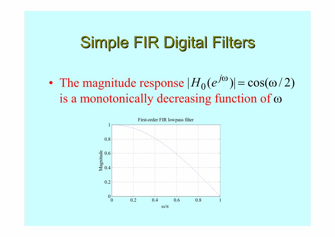
• The magnitude response
is a monotonically decreasing function of ω)2/cos(|)(| 0 ω=ωjeH
0 0.2 0.4 0.6 0.8 10
0.2
0.4
0.6
0.8
1
ω/π
Magnitude
First-order FIR lowpass filter

Simple FIR Digital FiltersSimple FIR Digital Filters
• The frequency at which
is of practical interest since here the gain in dB is
since the DC gain is
cω=ω
)(2
1)( 0
00jjeHeH c =ω
dB32log20)(log20 100
10 −≅−= jeH
)(log20)ω(Gω
10cj
c eH=
0)(log20 0
10 =jeH

Simple FIR Digital FiltersSimple FIR Digital Filters
• Thus, the gain G(ω) at is approximately 3 dB less than the gain at ω=0
• As a result, is called the 3-dB cutoff
frequency
• To determine the value of we set
which yields
cω=ω
cω
cω
2/π=ωc
2
1220 )2/(cos|)(| =ω=ω
cj ceH

Simple FIR Digital FiltersSimple FIR Digital Filters
• The 3-dB cutoff frequency can be
considered as the passband edge frequency
• As a result, for the filter the passband
width is approximately π/2
• The stopband is from π/2 to π
• Note: has a zero at or ω = π,which is in the stopband of the filter
cω
)(zH0
)(zH0 1−=z

Simple FIR Digital FiltersSimple FIR Digital Filters
• A cascade of the simple FIR filter
results in an improved lowpass frequency
response as illustrated below for a cascade
of 3 sections
)()( 1
21
0 1 −+= zzH
0 0.2 0.4 0.6 0.8 10
0.2
0.4
0.6
0.8
1
ω/π
Magnitude
First-order FIR lowpass filter cascade

Simple FIR Digital FiltersSimple FIR Digital Filters
• The 3-dB cutoff frequency of a cascade of
M sections is given by
• For M = 3, the above yields
• Thus, the cascade of first-order sections
yields a sharper magnitude response but at
the expense of a decrease in the width of the
passband
)2(cos2 2/11 Mc
−−=ω
π=ω 302.0c

Simple FIR Digital FiltersSimple FIR Digital Filters
• A better approximation to the ideal lowpass
filter is given by a higher-order Moving
Average (MA) filter
• Signals with rapid fluctuations in sample
values are generally associated with high-
frequency components
• These high-frequency components are
essentially removed by an MA filter
resulting in a smoother output waveform

Simple FIR Digital FiltersSimple FIR Digital Filters
Highpass FIR Digital Filters
• The simplest highpass FIR filter is obtained
from the simplest lowpass FIR filter by
replacing z with
• This results in
)()( 1
2
11 1 −−= zzH
z−

Simple FIR Digital FiltersSimple FIR Digital Filters
• Corresponding frequency response is given
by
whose magnitude response is plotted below
)2/sin()( 2/1 ω= ω−ω jj ejeH
0 0.2 0.4 0.6 0.8 10
0.2
0.4
0.6
0.8
1
ω/π
Magnitude
First-order FIR highpass filter

Simple FIR Digital FiltersSimple FIR Digital Filters
• The monotonically increasing behavior of
the magnitude function can again be
demonstrated by examining the pole-zero
pattern of the transfer function
• The highpass transfer function has a
zero at z = 1 or ω = 0 which is in the
stopband of the filter
)(zH1
)(zH1

Simple FIR Digital FiltersSimple FIR Digital Filters
• Improved highpass magnitude response can
again be obtained by cascading several
sections of the first-order highpass filter
• Alternately, a higher-order highpass filter of
the form
is obtained by replacing z with in the
transfer function of an MA filter
z−
nMn
n
MzzH −−
=∑ −= 10
11 1)()(

Simple IIR Digital FiltersSimple IIR Digital Filters
Lowpass IIR Digital Filters
• A first-order causal lowpass IIR digital
filter has a transfer function given by
where |α| < 1 for stability• The above transfer function has a zero at
i.e., at ω = π which is in the stopband
α−
+α−= −
−
1
1
1
1
2
1)(
z
zzHLP
1−=z

Simple IIR Digital FiltersSimple IIR Digital Filters
• has a real pole at z = α
• As ω increases from 0 to π, the magnitude
of the zero vector decreases from a value of
2 to 0, whereas, for a positive value of α, the magnitude of the pole vector increases
from a value of to
• The maximum value of the magnitude
function is 1 at ω = 0, and the minimum
value is 0 at ω = π
α−1 α+1
)(zHLP

Simple IIR Digital FiltersSimple IIR Digital Filters
• i.e.,
• Therefore, is a monotonically
decreasing function of ω from ω = 0 to ω = πas indicated below
0|)(|,1|)(| 0 == πjLP
jLP eHeH
|)(| ωjLP eH
0 0.2 0.4 0.6 0.8 10
0.2
0.4
0.6
0.8
1
ω/π
Magnitude
α = 0.8α = 0.7α = 0.5
10-2
10-1
100
-20
-15
-10
-5
0
ω/π
Gain, dB α = 0.8
α = 0.7α = 0.5

Simple IIR Digital FiltersSimple IIR Digital Filters
• The squared magnitude function is given by
• The derivative of with respect
to ω is given by
)cos21(2
)cos1()1(|)(|
2
22
ωα−α+
ω+α−=ωj
LP eH
2|)(| ωjLP eH
22
222
)cos21(2
sin)21()1(|)(|
α+ωα−
ωα+α+α−−=
ω
ω
d
eHd jLP

Simple IIR Digital FiltersSimple IIR Digital Filters
in the range
verifying again the monotonically decreasing
behavior of the magnitude function
• To determine the 3-dB cutoff frequency we set
in the expression for the squared magnitude
function resulting in
0ω/)(2
ω ≤deHd j
LP π≤ω≤0
2
1)(2
ω =cj
LP eH

Simple IIR Digital FiltersSimple IIR Digital Filters
or
which when solved yields
• The above quadratic equation can be solved for α yielding two solutions
2
1
)cos21(2
)cos1()1(2
2
=ωα−α+
ω+α−
c
c
cc ωα−α+=ω+α− cos21)cos1()1( 22
21
2cos
α+
α=ωc

Simple IIR Digital FiltersSimple IIR Digital Filters
• The solution resulting in a stable transfer
function is given by
• It follows from
that is a BR function for |α| < 1
)cos21(2
)cos1()1(|)(|
2
22
ωα−α+
ω+α−=ωj
LP eH
)(zHLP
)(zHLP
c
cωω−
=αcossin1

Simple IIR Digital FiltersSimple IIR Digital Filters
Highpass IIR Digital Filters
• A first-order causal highpass IIR digital filter
has a transfer function given by
where |α| < 1 for stability• The above transfer function has a zero at z = 1
i.e., at ω = 0 which is in the stopband
• It is a BR function for |α| < 1
−−+
= −
−
1
1
1
1
2
1)(
z
zzHHP α
α

Simple IIR Digital FiltersSimple IIR Digital Filters
• Its 3-dB cutoff frequency is given by
which is the same as that of
• Magnitude and gain responses of
are shown below
cc ωω−=α cos/)sin1(
cω
)(zHLP
)(zHHP
10-2
10-1
100
-20
-15
-10
-5
0
ω/π
Gain, dB
α = 0.8α = 0.7α = 0.5
0 0.2 0.4 0.6 0.8 10
0.2
0.4
0.6
0.8
1
ω/π
Magnitude
α = 0.8α = 0.7α = 0.5

Example 1-First Order HP Filter
• Design a first-order highpass filter with a 3-
dB cutoff frequency of 0.8π
• Now,
and
• Therefore
587785.0)8.0sin()sin( =π=ωc80902.0)8.0cos( −=π
5095245.0cos/)sin1( −=ωω−=α cc

Example 1-First Order HP Filter
• Therefore,
+
−=
−
−
1
1
509524501
12452380
z
z
..
−
−+=
−
−
1
1
1
1
2
1
z
zzHHP
α
α)(

Simple IIR Digital FiltersSimple IIR Digital Filters
Bandpass IIR Digital Filters
• A 2nd-order bandpass digital transfer
function is given by
• Its squared magnitude function is2)( ωj
BP eH
]2cos2cos)1(2)1(1[2
)2cos1()1(2222
2
ωα+ωα+β−α+α+β+
ω−α−=
α+α+β−
−α−= −−
−
21
2
)1(1
1
2
1)(
zz
zzHBP
Simple IIR Digital FiltersSimple IIR Digital Filters
• goes to zero at ω = 0 and ω = π• It assumes a maximum value of 1 at ,
called the center frequency of the bandpass
filter, where
• The frequencies and where
becomes 1/2 are called the 3-dB cutoff
frequencies
2|)(| ωjBP eH
2|)(| ωjBP eH
oω=ω
)(cos 1 β=ω −o
1cω 2cω

Simple IIR Digital FiltersSimple IIR Digital Filters
• The difference between the two cutoff
frequencies, assuming is called
the 3-dB bandwidth and is given by
• The transfer function is a BR
function if |α| < 1 and |β| < 1
12 cc ω>ω
)(zHBP
112 cos−=ω−ω= ccwB
α+
α21
2

Simple IIR Digital FiltersSimple IIR Digital Filters
• Plots of are shown below|)(| ωjBP eH
0 0.2 0.4 0.6 0.8 10
0.2
0.4
0.6
0.8
1
ω/π
Magnitude
β = 0.34
α = 0.8α = 0.5α = 0.2
0 0.2 0.4 0.6 0.8 10
0.2
0.4
0.6
0.8
1
ω/π
Magnitude
α = 0.6
β = 0.8β = 0.5β = 0.2

Example 2-Second Order BP Filter
• Design a 2nd order bandpass digital filter with center frequency at 0.4π and a 3-dB bandwidth of 0.1π
• Here
and
• The solution of the above equation yields:α = 1.376382 and α = 0.72654253
9510565.0)1.0cos()cos(1
22
=π==α+
αwB
309017.0)4.0cos()cos( =π=ω=β o

Example 2-Second Order BP Filter
• The corresponding transfer functions are
and
• The poles of are at z = 0.3671712 and have a magnitude > 1
±114256361.j
21
2
376381734342401
1188190
−−
−
+−
−−=
zz
zzHBP
...)('
21
2
72654253053353101
1136730
−−
−
+−
−=
zz
zzHBP
...)("
)(' zHBP

Example 2-Second Order BP Filter
• Thus, the poles of are outside the
unit circle making the transfer function
unstable
• On the other hand, the poles of are
at z = and have a
magnitude of 0.8523746
• Hence, is BIBO stable
)(' zHBP
)(" zHBP8095546026676550 .. j±
)(" zHBP

Example 2-Second Order BP Filter
• Figures below show the plots of the
magnitude function and the group delay of
)(" zHBP
0 0.2 0.4 0.6 0.8 10
0.2
0.4
0.6
0.8
1
ω/π
Magnitude
0 0.2 0.4 0.6 0.8 1-1
0
1
2
3
4
5
6
7
ω/π
Group delay, samples

Simple IIR Digital FiltersSimple IIR Digital Filters
Bandstop IIR Digital Filters
• A 2nd-order bandstop digital filter has a
transfer function given by
• The transfer function is a BR
function if |α| < 1 and |β| < 1
α+α+β−
+β−α+= −−
−−
21
21
)1(1
21
2
1)(
zz
zzzHBS
)(zHBS

Simple IIR Digital FiltersSimple IIR Digital Filters
• Its magnitude response is plotted below
0 0.2 0.4 0.6 0.8 10
0.2
0.4
0.6
0.8
1
ω/π
Magnitude
α = 0.8α = 0.5α = 0.2
0 0.2 0.4 0.6 0.8 10
0.2
0.4
0.6
0.8
1
ω/π
Magnitude
β = 0.8β = 0.5β = 0.2

Simple IIR Digital FiltersSimple IIR Digital Filters
• Here, the magnitude function takes the
maximum value of 1 at ω = 0 and ω = π• It goes to 0 at , where , called the
notch frequency, is given by
• The digital transfer function is more
commonly called a notch filter
oω=ω oω
)(cos 1 β=ω −o
)(zHBS

Simple IIR Digital FiltersSimple IIR Digital Filters
• The frequencies and where
becomes 1/2 are called the 3-dB cutoff
frequencies
• The difference between the two cutoff
frequencies, assuming is called
the 3-dB notch bandwidth and is given by
2|)(| ωjBS eH1cω 2cω
12 cc ω>ω
112 cos−=ω−ω= ccwB
α+
α21
2

Simple IIR Digital FiltersSimple IIR Digital Filters
Higher-Order IIR Digital Filters
• By cascading the simple digital filters
discussed so far, we can implement digital
filters with sharper magnitude responses
• Consider a cascade of K first-order lowpass
sections characterized by the transfer
function
α−
+α−= −
−
1
1
1
1
2
1)(
z
zzHLP
Simple IIR Digital FiltersSimple IIR Digital Filters
• The overall structure has a transfer function
given by
• The corresponding squared-magnitude
function is given by
K
LPz
zzG
−+−
= −
−
1
1
α1
1
2
α1)(
K
jLP eG
ωα−α+
ω+α−=ω
)cos21(2
)cos1()1(|)(|
2
22

Simple IIR Digital FiltersSimple IIR Digital Filters
• To determine the relation between its 3-dB
cutoff frequency and the parameter α, we set
which when solved for α, yields for a stable :
cω
2
1
)cos21(2
)cos1()1(2
2
=
ωα−α+
ω+α−K
c
c
)(zGLP
c
cc
C
CCC
ω+−−ω−ω−+
=αcos1
2sincos)1(1 2

Simple IIR Digital FiltersSimple IIR Digital Filters
where
• It should be noted that the expression given
above reduces to
for K = 1
KKC /)( 12 −=
c
cωω−
=αcossin1

• Design a lowpass filter with a 3-dB cutoff
frequency at using a single first-order
section and a cascade of 4 first-order sections, and
compare their gain responses
• For the single first-order lowpass filter we have
π=ω 4.0c
1584.0)4.0cos(
)4.0sin(1
cos
sin1=
ππ+
=ωω+
=αc
c
Example 3-Design of an LP Filter

Example 3-Design of an LP Filter
• For the cascade of 4 first-order sections, we
substitute K = 4 and get
• Next we compute
6818122 4141 ./)(/)( === −− KKC
c
cc
C
CCC
ω+−−ω−ω−+
=αcos1
2sincos)1(1 2
)4.0cos(6818.11
)6818.1()6818.1(2)4.0sin()4.0cos()6818.11(1 2
π+−−π−π−+
=
2510.−=

Example 3-Design of an LP Filter
• The gain responses of the two filters are
shown below
• As can be seen, cascading has resulted in a
sharper roll-off in the gain response
10-2
10-1
100
-20
-15
-10
-5
0
ω/π
Gain, dB
K=4
K=1Passband details
10-2
10-1
100
-4
-2
0
ω/π
Gain, dB K=1
K=4

Comb FiltersComb Filters
• The simple filters discussed so far are
characterized either by a single passband
and/or a single stopband
• There are applications where filters with
multiple passbands and stopbands are required
• The comb filter is an example of such filters

Comb FiltersComb Filters
• In its most general form, a comb filter has a
frequency response that is a periodic
function of ω with a period 2π/L, where L is a positive integer
• If H(z) is a filter with a single passband
and/or a single stopband, a comb filter can
be easily generated from it by replacing
each delay in its realization with L delays
resulting in a structure with a transfer
function given by )()( LzHzG =

Comb FiltersComb Filters
• If exhibits a peak at , then
will exhibit L peaks at ,
in the frequency range
• Likewise, if has a notch at ,
then will have L notches at ,
in the frequency range
• A comb filter can be generated from either
an FIR or an IIR prototype filter
|)(| ωjeH
|)(| ωjeH
|)(| ωjeG
|)(| ωjeGpω
oω
Lkp /ω
Lko /ω
10 −≤≤ Lk
10 −≤≤ Lk
π<ω≤ 20
π<ω≤ 20

Comb FiltersComb Filters
• For example, the comb filter generated from
the prototype lowpass FIR filter
has a transfer function
• has L notches
at ω = (2k+1)π/L and Lpeaks at ω = 2π k/L,
)( 1
21 1 −+ z=)(zH0
)()()( LL zzHzG −+== 121
00
10 −≤≤ Lk , in thefrequency range
π<ω≤ 20
|)(| 0ωjeG
0 0.5 1 1.5 20
0.2
0.4
0.6
0.8
1
ω/π
Magnitude
Comb filter from lowpass prototype

Comb FiltersComb Filters
• Furthermore, the comb filter generated from
the prototype highpass FIR filter
has a transfer function
• has L peaks
at ω = (2k+1)π/L and Lnotches at ω = 2π k/L,
|)(| 1ωjeG
)( 1
21 1 −− z=)(zH1
)()()( LL zzHzG −−== 121
11
10 −≤≤ Lk , in thefrequency range
π<ω≤ 200 0.5 1 1.5 2
0
0.2
0.4
0.6
0.8
1
ω/π
Magnitude
Comb filter from highpass prototype
Comb FiltersComb Filters
• Depending on applications, comb filters with other
types of periodic magnitude responses can be
easily generated by appropriately choosing the
prototype filter
• For example, theM-point moving average filter
has been used as a prototype
)1(
1)(
1−
−
−−
=zM
zzH
M

Comb FiltersComb Filters
• This filter has a peak magnitude at ω = 0, and
notches at ,
• The corresponding comb filter has a transfer
function
whose magnitude has L peaks at ,
and notches at
,
1−M M/2 lπ=ω 11 −≤≤ Ml
)1(
1)(
L
LM
zM
zzG
−
−
−−
=
Lk/2π=ω10 −≤≤ Lk )( 1−ML
LMk/2π=ω )( 11 −≤≤ MLk

AllpassAllpass Transfer FunctionsTransfer Functions
Definition
• An IIR transfer function A(z) with unity
magnitude response for all frequencies, i.e.,
is called an allpass transfer function
• An M-th order causal real-coefficient
allpass transfer function is of the form
ω=ω allfor,1|)(| 2jeA
M
M
M
M
MM
MMM
zdzdzd
zzdzddzA
−+−−
−
−+−−−
++++++++
±=1
1
1
1
1
1
1
1
1)(
K
K

AllpassAllpass Transfer FunctionsTransfer Functions
• If we denote the denominator polynomials of
as :
then it follows that can be written as:
• Note from the above that if is a pole of a
real coefficient allpass transfer function, then it
has a zero at
)(zDM)(zAMM
M
M
MM zdzdzdzD −+−−
− ++++= 1
1
1
11)( K
)(zAM
)(
)()(
zD
zDzM
M
MM
zA1−−
±=
φ= jrez
φ−= jr ez 1

AllpassAllpass Transfer FunctionsTransfer Functions
• The numerator of a real-coefficient allpass
transfer function is said to be themirror-
image polynomial of the denominator, and
vice versa
• We shall use the notation to denote
the mirror-image polynomial of a degree-M
polynomial , i.e.,
)(zDM~
)(zDM
)()( zDzzD MM
M−=
~

AllpassAllpass Transfer FunctionsTransfer Functions
• The expression
implies that the poles and zeros of a real-
coefficient allpass function exhibitmirror-
image symmetry in the z-plane
)(
)()(
zD
zDzM
M
MM
zA1−−
±=
321
321
32.018.04.01
4.018.02.0)( −−−
−−−
−+++++−
=zzz
zzzzA
-1 0 1 2 3
-1.5
-1
-0.5
0
0.5
1
1.5
Real Part
Imaginary Part

AllpassAllpass Transfer FunctionsTransfer Functions
• To show that we observe that
• Therefore
• Hence,
)(
)()(
1
1
−− ±=
zD
zDzzA
M
M
M
M
)(
)(
)(
)()()(
1
11
−
−−− =
zD
zDz
zD
zDzzAzA
M
M
M
M
M
M
MM
1|)(| =ωjM eA
1)()(|)(| 12 == ω=−ω
jezMMj
M zAzAeA
AllpassAllpass Transfer FunctionsTransfer Functions
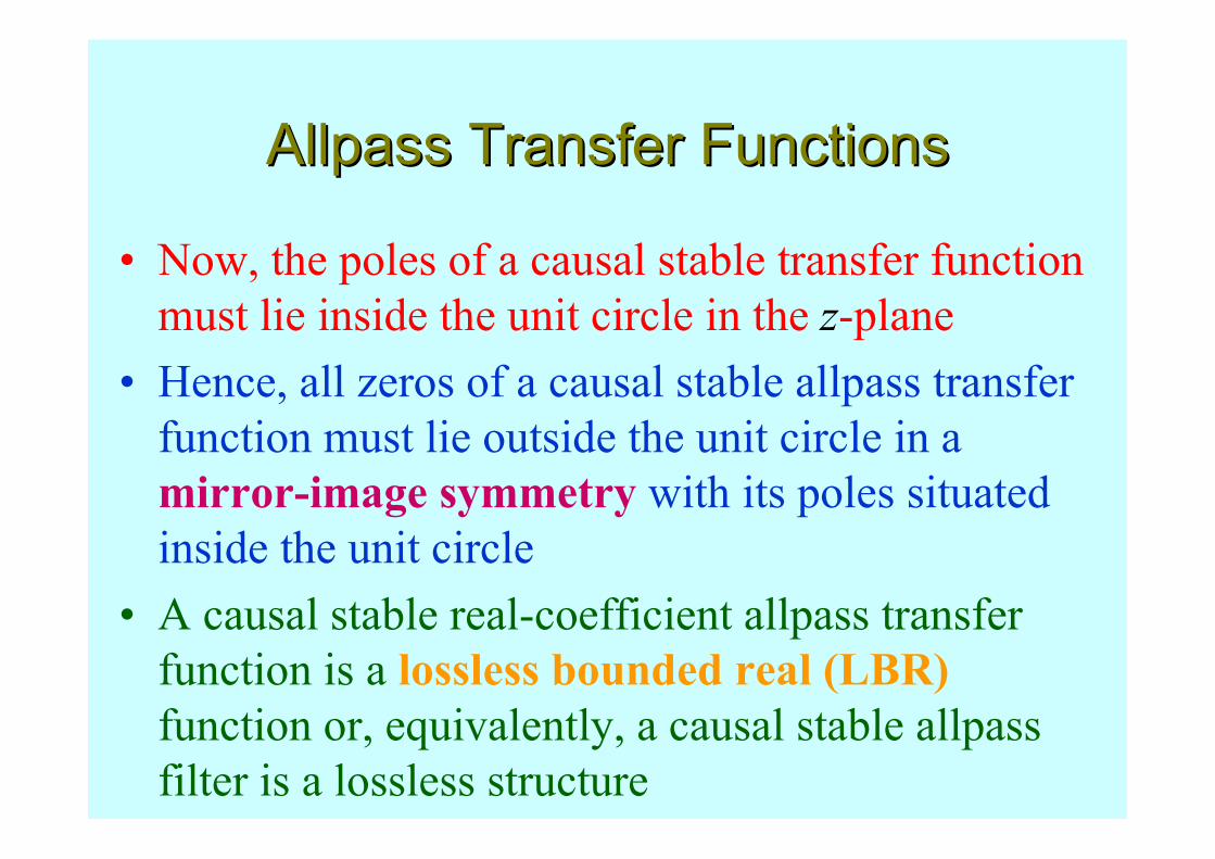
• Now, the poles of a causal stable transfer function
must lie inside the unit circle in the z-plane
• Hence, all zeros of a causal stable allpass transfer
function must lie outside the unit circle in a
mirror-image symmetry with its poles situated
inside the unit circle
• A causal stable real-coefficient allpass transfer
function is a lossless bounded real (LBR)
function or, equivalently, a causal stable allpass
filter is a lossless structure

AllpassAllpass Transfer FunctionsTransfer Functions
• The magnitude function of a stable allpass
function A(z) satisfies:
• Let τ(ω) denote the group delay function of an allpass filter A(z), i.e.,
<>==><
1for1
1for1
1for1
z
z
z
zA
,
,
,
)(
)]([)( ωθ−=ωτω cd
d

AllpassAllpass Transfer FunctionsTransfer Functions
• The unwrapped phase function of a
stable allpass function is a monotonically
decreasing function of ω so that τ(ω) iseverywhere positive in the range 0 < ω < π
• The group delay of an M-th order stable
real-coefficient allpass transfer function
satisfies:
)(ωθc
π=ω∫ ωτπ
Md0
)(

AllpassAllpass Transfer FunctionTransfer Function
A Simple Application
• A simple but often used application of an allpass filter is as a delay equalizer
• Let G(z) be the transfer function of a digital filter designed to meet a prescribed magnitude response
• The nonlinear phase response of G(z) can be corrected by cascading it with an allpassfilter A(z) so that the overall cascade has a constant group delay in the band of interest

AllpassAllpass Transfer FunctionTransfer Function
• Since , we have
• Overall group delay is the given by the sum
of the group delays of G(z) and A(z)
1|)(| =ωjeA
|)(||)()(| ωωω = jjj eGeAeG
G(z) A(z)

MinimumMinimum--Phase and MaximumPhase and Maximum--
Phase Transfer FunctionsPhase Transfer Functions
• Consider the two 1st-order transfer functions:
• Both transfer functions have a pole inside the
unit circle at the same location and are
stable
• But the zero of is inside the unit circle
at , whereas, the zero of is at
situated in a mirror-image symmetry
11121 <<== +
+++ bazHzH
azbz
azbz ,,)(,)(
az −=
bz −=
bz 1−=
)(zH1
)(zH2

MinimumMinimum--Phase and MaximumPhase and Maximum--
Phase Transfer FunctionsPhase Transfer Functions
• Figure below shows the pole-zero plots of
the two transfer functions
)(1 zH )(2 zH

MinimumMinimum--Phase and MaximumPhase and Maximum--
Phase Transfer FunctionsPhase Transfer Functions
• However, both transfer functions have an
identical magnitude as
• The corresponding phase functions are
)()()()( 1
22
1
11
−− = zHzHzHzH
ωcos
ωsintan
ωcos1
ωsintan)](arg[ 11ω
2 +−
+= −−
ab
beH j
ωcos
ωsintan
ωcos
ωsintan)](arg[ 11ω
1 +−
+= −−
abeH j

MinimumMinimum--Phase and MaximumPhase and Maximum--
Phase Transfer FunctionsPhase Transfer Functions
• Figure below shows the unwrapped phase
responses of the two transfer functions for
a=0.8 and b=-0.5
0 0.2 0.4 0.6 0.8 1-4
-3
-2
-1
0
1
2
ω/π
Phase, degrees
H1(z)
H2(z)

MinimumMinimum--Phase and MaximumPhase and Maximum--
Phase Transfer FunctionsPhase Transfer Functions
• From this figure it follows that has
an excess phase lag with respect to
• Generalizing the above result, we can show
that a causal stable transfer function with all
zeros outside the unit circle has an excess
phase compared to a causal transfer
function with identical magnitude but
having all zeros inside the unit circle
)(2 zH
)(1 zH

MinimumMinimum--Phase and MaximumPhase and Maximum--
Phase Transfer FunctionsPhase Transfer Functions
• A causal stable transfer function with all zeros
inside the unit circle is called aminimum-phase
transfer function
• A causal stable transfer function with all zeros
outside the unit circle is called amaximum-
phase transfer function
• Any nonminimum-phase transfer function can be
expressed as the product of a minimum-phase
transfer function and a stable allpass transfer
function

Complementary Transfer FunctionsComplementary Transfer Functions
• A set of digital transfer functions with
complementary characteristics often finds
useful applications in practice
• Four useful complementary relations are
described next along with some applications

Complementary Transfer FunctionsComplementary Transfer Functions
Delay-Complementary Transfer Functions
• A set of L transfer functions, ,
, is defined to be delay-
complementary of each other if the sum of
their transfer functions is equal to some
integer multiple of unit delays, i.e.,
where is a nonnegative integer
)}({ zHi10 −≤≤ Li
0,)(1
0
≠ββ= −−
=∑ onL
ii zzH
on

Complementary Transfer FunctionsComplementary Transfer Functions
• A delay-complementary pair
can be readily designed if one of the pairs is
a known Type 1 FIR transfer function of
odd length
• Let be a Type 1 FIR transfer function
of lengthM = 2K+1
• Then its delay-complementary transfer
function is given by
)}(),({ 10 zHzH
)()( 01 zHzzH K −= −
)(0 zH

Complementary Transfer FunctionsComplementary Transfer Functions
• Let the magnitude response of be
equal to in the passband and less than
or equal to in the stopband where and
are very small numbers
• Now the frequency response of can be
expressed as
where is the amplitude response
)(0 zH
pδ±1
sδ pδ
sδ)(0 zH
)()( 00 ω= ω−ω HeeH jKj ~
)(0 ωH~
Complementary Transfer FunctionsComplementary Transfer Functions
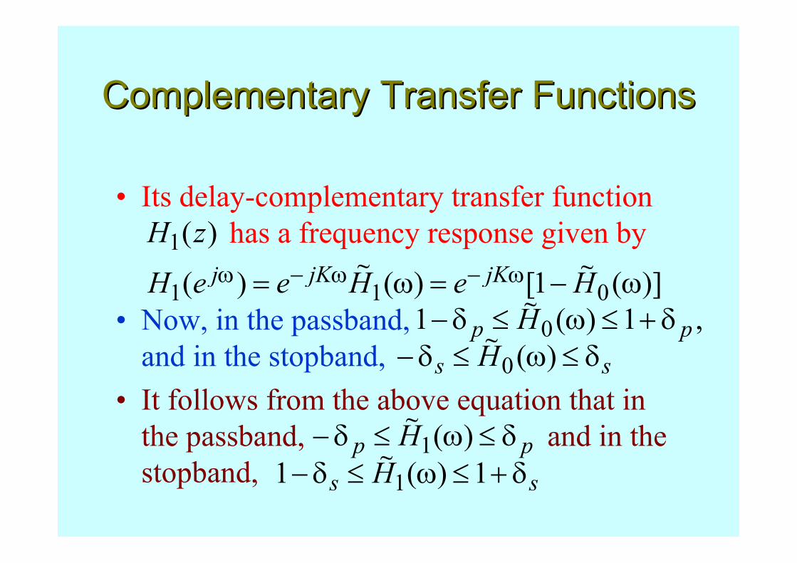
• Its delay-complementary transfer function
has a frequency response given by
• Now, in the passband,
and in the stopband,
• It follows from the above equation that in
the passband, and in the
stopband,
)(1 zH
)](1[)()( 011 ω−=ω= ω−ω−ω HeHeeH jKjKj ~ ~
,1)(1 0 pp H δ+≤ω≤δ−~
ss H δ≤ω≤δ− )(0~
pp H δ≤ω≤δ− )(1~
ss H δ+≤ω≤δ− 1)(1 1~

Complementary Transfer FunctionsComplementary Transfer Functions
• As a result, has a complementary
magnitude response characteristic, with a
stopband exactly identical to the passband
of , and a passband that is exactly
identical to the stopband of
• Thus, if is a lowpass filter, will
be a highpass filter, and vice versa
)(1 zH
)(0 zH
)(0 zH
)(1 zH)(0 zH

Complementary Transfer FunctionsComplementary Transfer Functions
• At frequency at which
the gain responses of both filters are 6 dB
below their maximum values
• The frequency is thus called the 6-dB
crossover frequencyoω
oω
5.0)()( 10 =ω=ω oo HH~~

Example 4
• Consider the Type 1 bandstop transfer function
• Its delay-complementary Type 1 bandpass transfer
function is given by
)45541()1(64
1)( 121084242 −−−−−− +−++−+= zzzzzzzHBS
)45541()1(64
1 121084242 −−−−−− +++++−−= zzzzzz
)()( 10 zHzzH BSBP −= −

Example 4
• Plots of the magnitude responses of
and are shown below
)(zHBS)(zHBP
0 0.2 0.4 0.6 0.8 10
0.2
0.4
0.6
0.8
1
ω/π
Magnitude
HBS(z) H
BP(z)

Complementary Transfer FunctionsComplementary Transfer Functions
Allpass Complementary Filters
• A set of M digital transfer functions, ,
, is defined to be allpass-
complementary of each other, if the sum of
their transfer functions is equal to an allpass
function, i.e.,
)}({ zHi10 −≤≤ Mi
)()(1
0
zAzHM
ii =∑
−
=

Complementary Transfer FunctionsComplementary Transfer Functions
Power-Complementary Transfer Functions
• A set of M digital transfer functions, ,
, is defined to be power-
complementary of each other, if the sum of
their square-magnitude responses is equal to
a constant K for all values of ω, i.e.,
)}({ zHi10 −≤≤ Mi
ω=∑−
=
ω allfor,)(1
0
2KeH
M
i
ji

Complementary Transfer FunctionsComplementary Transfer Functions
• By analytic continuation, the above
property is equal to
for real coefficient
• Usually, by scaling the transfer functions,
the power-complementary property is
defined for K = 1
)(zHi
ω=∑−
=
− allfor,)()(1
0
1 KzHzHM
iii

Complementary Transfer FunctionsComplementary Transfer Functions
• For a pair of power-complementary transfer
functions, and , the frequency
where , is
called the cross-over frequency
• At this frequency the gain responses of both
filters are 3-dB below their maximum
values
• As a result, is called the 3-dB cross-
over frequency
oω
oω
)(0 zH )(1 zH
5.0|)(||)(| 21
20 == ωω oo jj eHeH

Complementary Transfer FunctionsComplementary Transfer Functions
• Consider the two transfer functions
and given by
where and are stable allpass
transfer functions
• Note that
• Hence, and are allpass
complementary
)(0 zH
)(1 zH
)]()([)( 1021
0 zAzAzH +=
)(0 zA )(1 zA
)]()([)( 1021
1 zAzAzH −=
)()()( 010 zAzHzH =+
)(0 zH )(1 zH
Complementary Transfer FunctionsComplementary Transfer Functions
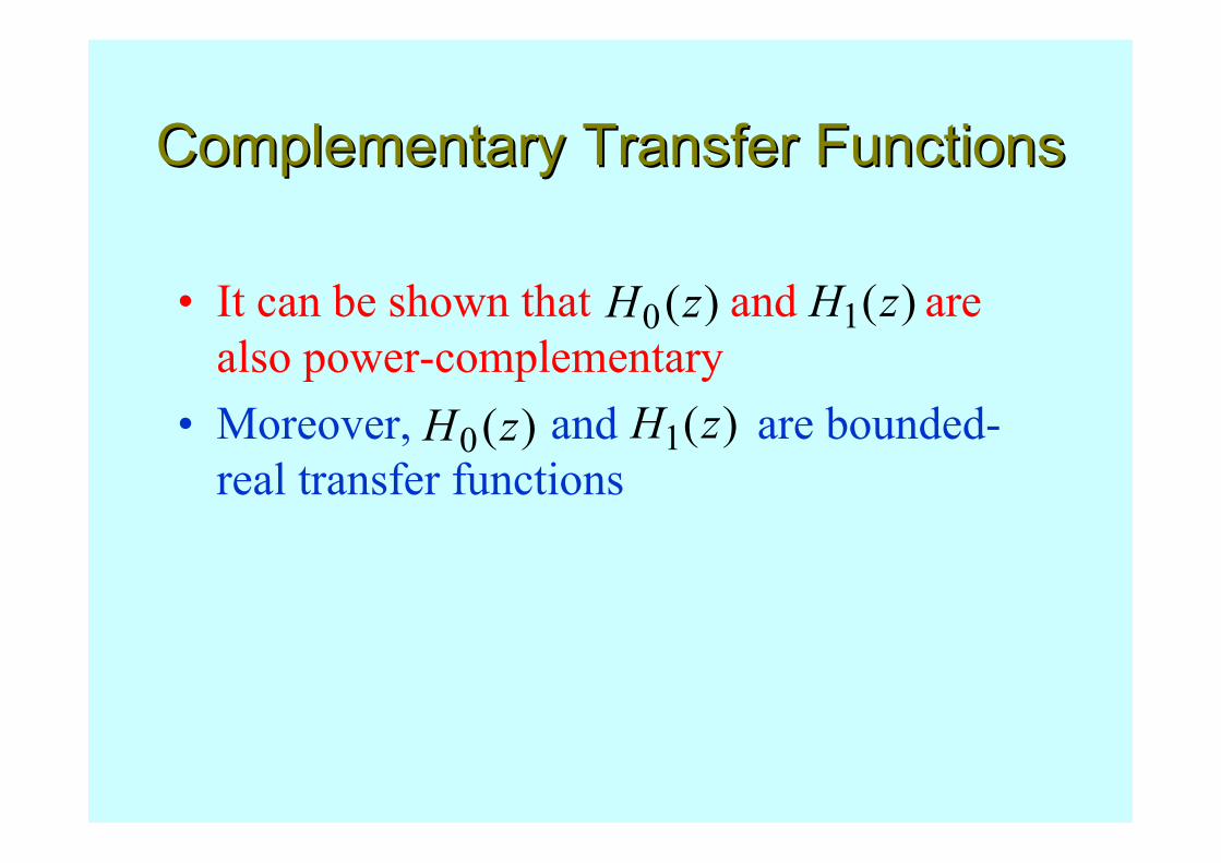
• It can be shown that and are
also power-complementary
• Moreover, and are bounded-
real transfer functions
)(0 zH )(1 zH
)(0 zH )(1 zH

Complementary Transfer FunctionsComplementary Transfer Functions
Doubly-Complementary Transfer Functions
• A set of M transfer functions satisfying both
the allpass complementary and the power-
complementary properties is known as a
doubly-complementary set

Complementary Transfer FunctionsComplementary Transfer Functions
• A pair of doubly-complementary IIR
transfer functions, and , with a
sum of allpass decomposition can be simply
realized as indicated below
)(0 zH )(1 zH
+
+)(1 zA
)(0 zA
)(zX
)(0 zY
)(1 zY1−
2/1
)(
)(00 )(
zX
zYzH =
)(
)(11 )(
zX
zYzH =

Example 5
• The first-order lowpass transfer function
can be expressed as
where
= −
−
α−+α−
1
1
1
1
2
1)(z
zLP zH
)]()([)( 102
1
11
2
11
1
zAzAzHz
zLP +
= =
α−+α−+ −
−
1
1
11
)( −
−
α−+α−=z
zzA,)( 10 =zA

Example 5
• Its power-complementary highpass transfer
function is thus given by
• The above expression is precisely the first-
order highpass transfer function described
earlier
=− −
−
α−+α−−=
1
1
11
2
1102
1 )]()([)(z
zHP zAzAzH
= −
−
α−−α+
1
1
1
1
2
1
z
z

Complementary Transfer FunctionsComplementary Transfer Functions
• Figure below demonstrates the allpass
complementary property and the power
complementary property of and)(zHLP)(zHHP
0 0.2 0.4 0.6 0.8 10
0.2
0.4
0.6
0.8
1
ω/π
Magnitude
|HHP
(ejω)|
|HLP(ejω)|
|HLP(ejω) + H
HP(ejω)|
0 0.2 0.4 0.6 0.8 10
0.2
0.4
0.6
0.8
1
ω/π
Magnitude
|HHP(ejω)|2
|HLP(ejω)|2
|HLP(ejω)|2 + |H
HP(ejω)|2

Complementary Transfer FunctionsComplementary Transfer Functions
Power-Symmetric Filters
• A real-coefficient causal digital filter with a
transfer function H(z) is said to be a power-
symmetric filter if it satisfies the condition
where K > 0 is a constant
KzHzHzHzH =−−+ −− )()()()( 11

Complementary Transfer FunctionsComplementary Transfer Functions
• It can be shown that the gain function G(ω) of a power-symmetric transfer function at ω= π is given by
• If we define , then it follows
from the definition of the power-symmetric
filter that H(z) and G(z) are power-
complementary as
constanta)()()()( 11 =+ −− zGzGzHzH
)()( zHzG −=
dBK 3log10 10 −

Complementary Transfer FunctionsComplementary Transfer Functions
Conjugate Quadratic Filter
• If a power-symmetric filter has an FIR
transfer function H(z) of order N, then the
FIR digital filter with a transfer function
is called a conjugate quadratic filter of
H(z) and vice-versa
)()( 11 −−= zHzzG

Complementary Transfer FunctionsComplementary Transfer Functions
• It follows from the definition that G(z) is
also a power-symmetric causal filter
• It also can be seen that a pair of conjugate
quadratic filters H(z) and G(z) are also
power-complementary

Example 6
• Let
• We form
• H(z) is a power-symmetric transfer
function
)3621)(3621( 32321 zzzzzz ++−++−= −−−
)()()()( 11 −− −−+ zHzHzHzH
321 3621)( −−− ++−= zzzzH
)3621)(3621( 32321 zzzzzz −++−+++ −−−
)345043( 313 −− ++++= zzzz
100)345043( 313 =−−+−−+ −− zzzz

Digital TwoDigital Two--PairsPairs
• The LTI discrete-time systems considered
so far are single-input, single-output
structures characterized by a transfer
function
• Often, such a system can be efficiently
realized by interconnecting two-input, two-
output structures, more commonly called
two-pairs

Digital TwoDigital Two--PairsPairs
• Figures below show two commonly used
block diagram representations of a two-pair
• Here and denote the two outputs, and
and denote the two inputs, where the
dependencies on the variable z have been
omitted for simplicity
1Y 2Y
1X 2X
1Y
2Y
1X
2X1Y
1X 2Y
2X

Digital TwoDigital Two--PairsPairs
• The input-output relation of a digital two-
pair is given by
• In the above relation the matrix ττττ given by
is called the transfer matrix of the two-pair
=
2
1
2221
1211
2
1
X
X
tt
tt
Y
Y
=
2221
1211
tt
ttττττ

Digital TwoDigital Two--PairsPairs
• It follows from the input-output relation that
the transfer parameters can be found as
follows:
02
112
01
111
12 ==
==XX
X
Yt
X
Yt ,
02
222
01
221
12 ==
==XX
X
Yt
X
Yt ,

Digital TwoDigital Two--PairsPairs
• An alternative characterization of the two-
pair is in terms of its chain parameters as
where the matrix ΓΓΓΓ given by
is called the chain matrix of the two-pair
=
2
2
1
1
X
YDCBA
Y
X
=
DCBAΓΓΓΓ
- -

Digital TwoDigital Two--PairsPairs
• The relation between the transfer parameters and
the chain parameters are given by
A
Bt
At
A
BCADt
A
Ct −==
−== 22211211 ,
1,,
21
22112112
21
11
21
22
21
1t
ttttD
t
tC
t
tB
tA
−==−== ,,,

TwoTwo--Pair Interconnection SchemesPair Interconnection Schemes
Cascade Connection - ΓΓΓΓ-cascade
• Here
'1Y
'1X
"1Y
'2Y "
2Y"1X
"2X'
2X
''
''
DCBA
- -
""
""
DCBA
--
=
'2
'2
''
''
'1
'1
X
Y
DCBA
Y
X
=
"2
"2
""
""
"1
"1
X
Y
DCBA
Y
X

TwoTwo--Pair Interconnection SchemesPair Interconnection Schemes
• But from figure, and
• Substituting the above relations in the first
equation on the previous slide and
combining the two equations we get
• Hence,
'2
"1 YX = '
2"1 XY =
=
"2
"2
""
""
''
''
'1
'1
X
Y
DCBA
DCBA
Y
X
=
""
""
''
''
DCBA
DCBA
DCBA

TwoTwo--Pair Interconnection SchemesPair Interconnection Schemes
Cascade Connection - ττττ-cascade
• Here
'1Y'
1X"1Y
'2Y
"2Y
"1X
"2X
'2X
'22
'21
'12
'11
tt
tt
- - --
"22
"21
"12
"11
tt
tt
=
"2
"1
"22
"21
"12
"11
"2
"1
X
X
tt
tt
Y
Y

TwoTwo--Pair Interconnection SchemesPair Interconnection Schemes
• But from figure, and
• Substituting the above relations in the first
equation on the previous slide and
combining the two equations we get
• Hence,
'1
"1 YX = '
2"2 YX =
=
'2
'1
'22
'21
'12
'11
"22
"21
"12
"11
"2
"1
X
X
tt
tt
tt
tt
Y
Y
=
'22
'21
'12
'11
"22
"21
"12
"11
2221
1211
tt
tt
tt
tt
tt
tt

TwoTwo--Pair Interconnection SchemesPair Interconnection Schemes
Constrained Two-Pair
• It can be shown that
1Y
1X 2Y
2XG(z)
H(z)
)(
)()(
1
1
zGBA
zGDC
X
YzH
⋅+⋅+
==
)(1
)(
22
211211
zGt
zGttt
−+=