Lecture 7

Gradient and directional derivative (cont’d)

In the previous lecture, we showed that the rate of change of a function f(x, y) in the direction of a

vector u, called the directional derivative of f at a in the direction u, is simply the dot product of the

gradient vector ~∇f(a) with the unit direction vector u:

Duf(a) = ~∇f(a) · u =∂f

∂x(a)u1 +

∂f

∂y(a)u2. (1)

The gradient vector ~∇f(a) contains all the information necessary to compute the directional derivative

of f at a in any direction.

We then considered the “hotplate temperature function” f(x, y) = 50 − x2 − 2y2 and computed

the rate of change of temperature at the reference point (1,−1) – the location of an ant – in several

directions. We found that the direction u = (1,−1) was a good direction if the ant wanted to cool

itself, but the question remained: Is it the best direction? In order to answer this question, we should

return to Eq. (1).

Let’s rewrite the dot product in Eq. (1) as follows,

Duf(a) = ‖ ~∇f(a) ‖‖ u ‖ cos θ (2)

= ‖ ~∇f(a) ‖ cos θ,

where θ is the angle between the unit vector u and ~∇f(a). We have expressed the directional derivative

Duf(a) in terms of the magnitude of the gradient vector ~∇f(a) evaluated at a and the angle between

the gradient vector and the direction vector u. We have all that we need.

The function cos θ can assume all values between 1 and −1. Its maximum value 1 corresponds to

θ = 0. Its minimum value −1 corresponds to θ = π. It assumes the value of 0 at θ = ±π/2. This

leads to the following three special cases:

1. θ = 0. Then u points in the direction of ~∇f(a). In this case, the rate of change Duf assumes

its maximum (or most positive) value, ‖ ~∇f(a) ‖≥ 0. This is the direction of steepest ascent of

f at (a, b).

45

2. θ = π. Then u points in the direction of −~∇f(a). In this case, the rate of change Duf assumes

its minimum (or most negative) value, − ‖ ~∇f(a) ‖≤ 0. This is the direction of steepest descent

of f at (a, b).

3. θ = ±π/2. Then u points in a direction that is perpendicular to ~∇f(a). In this case, the rate of

change Duf is zero.

There are some noteworthy consequences of these consequences!

1. Directions in which the rate of change of f are zero must be tangent to the level curve of f that

passes through (a, b). Why? If you travel on a level curve, the value of f does not change. And

the instantaneous direction of motion at any point on this curve is the tangent vector to the

curve at that point.

2. The gradient vector ~∇f(a, b) must be perpendicular to the level curve of f that passes through

(a, b).

These results are sketched below.

through (x, y)

~∇f

−~∇f

direction of steepest descent of f

direction of steepest ascent of f

level set of f(x, y) passing

Example: We now return to the ant-hotplate problem f(x, y) = 50 − x2 − 2y2. Recall that the

gradient vector field of f is

~∇f(x, y) = −2xi − 4yj. (3)

And recall that the ant was situated at (a, b) = (1,−1). The question that remained unanswered in

the last lecture was, “In which direction should the ant start to travel in order to cool itself as quickly

as possible?” We now know the answer to this question - the ant should travel in the direction of

46

−~∇f(1,−1), the direction of steepest descent at (1,−1). This is the vector

~∇f(1,−1) = −2i + 4j. (4)

Note that this vector does not point directly at the origin, the hottest point on the plate, but this is

because of the elliptical nature of the level curves, as we’ll see below.

If we now consider all points (x, y) on the hotplate, the temperature function f(x, y) defines a

scalar field on this plate – you need only one number to characterize the temperature at a point.

Associated with this scalar field is the vector field defined by the gradient vector ~∇f(x, y). Why is

it a vector field? Because it is measuring rates of change of the scalar field – in particular, ~∇f(x, y)

defines (i) the direction of steepest ascent as well as (ii) the magnitude of the rate of change in that

direction. Magnitude + direction = vector.

The gradient field ~∇f(x, y) defined by the temperature function f(x, y) is sketched roughly in the

next figure. As expected, the vectors point “inward.”

x

y

Sketch of the gradient vector field ~∇f(x, y) = −2xi− 4yj.

The gradient field points inward because f(x, y) is increasing as we move toward (0, 0), at which

f achieves its global maximum: ~∇f(0, 0) = (0, 0). Notice that the magnitudes of the gradient vectors

decrease as we approach (0, 0) – this implies that the magnitudes of the rates of change are decreasing,

indicating that the graph of f is flattening out as we approach the local maximum (0, 0).

The relationship between the gradient vectors – as directions of steepest ascent – and level curves

– as contours of equal value – is clearly illustrated in the second figure below, in which both are plotted

for the hotplate temperature function.

47

x

y

direction f of steepest ascent of f(x, y)

level set f(x, y) = C

Sketch of gradient field vectors ~∇f(x, y) and level curves for the hotplate function f(x, y) = 50 − x2 − 2y2.

Actually, the ant – and nature, as we’ll see below – is more interested in the vector field −~∇f :

the direction of maximum decrease, or steepest descent, of the temperature function f(x, y). At each

point (x, y), the vector −~∇f(x, y) gives the best direction for which the ant to travel in order to cool

itself as quickly as possible. A sketch of this vector field, along with some level curves, is given below.

x

y

level set f(x, y) = C

direction f of steepest descent of f(x, y)

Sketch of gradient field vectors −~∇f(x, y) and level curves for the hotplate function f(x, y) = 50 − x2 − 2y2.

In fact, this vector field is quite relevant to the physical phenomenon of heat flow: Heat always

travels from a region of higher temperature to one of lower temperature in roughly the most efficient

manner. (We use the word “roughly” because the process of heat transfer involves the random collision

of molecules that leads to transfer of kinetic and rotational energy.) A simplified version of Fourier’s

“Law” of Cooling is as follows:

48

h = −κ~∇T (5)

Here, h is the “heat flux vector” that characterizes the heat flow, both in terms of direction and the

amount of heat going through a unit volume per unit time. T (x, y, z) is the temperature function and

κ is the thermal conductivity, a constant that is specific to the medium of interest. Once again, note

that heat flows in the direction of the negative gradient, i.e., the direction of steepest descent of the

temperature function T . And the greater the magnitude of ~∇T , i.e., the greater the rate of change of

T in this direction, the greater the flow of heat, which makes intuitive sense.

Notes:

1. The word “Law” was put in quotes since it is not a law, but rather a mathematical model of a

physical process. In the same way, as we’ll discuss later, Hooke’s “Law” for springs is not a law

but a simplified mathematical model.

2. The thermal conductivity κ above was assumed to be constant in this simplified form of Fourier’s

Law. In reality, κ may vary from region to region. As well, because of the microstructure of the

medium, i.e., the way that atoms in the medium are bound to each other, the conductivity may

be different in various directions – for example, it may be easier to flow in the x-direction than

in the y- and z-directions. For this reason, κ may have to be represented by a tensor. You will

encounter tensors in your third-year mathematical physics course.)

A few words on heat transfer and transport processes in general

In fact, heat transfer is a special case of a transport process – the movement of “something,” whether

it be heat, a chemical in solution, or bacteria in air – from regions of higher concentration to regions of

lower concentration. The transfer is described by a flux density vector field F that gives the direction

of motion at a point as well as the rate of transfer of the “something.”

Heat transfer is a special case of Fick’s Law of transport which states that the flux vector F points

in the direction of steepest descent of the concentration f of the “something” concerned, i.e.,

F(x, y, z) = −k~∇f(x, y, z), (6)

where k > 0 is a constant specific to the process and material being studied. Once again, the direction

49

of the flow is away from regions of higher concentration. This idea will be important in your future

studies of transport processes.

The gradient vector and directional derivatives in higher dimensions

The definition of the gradient vector given earlier for functions of two variables f(x, y) extends in a

natural way to scalar valued functions f : Rn → R where n ≥ 2:

~∇f(x) =∂f

∂x1(x)e1 + · · · +

∂f

∂xn(x)en, (7)

where x = (x1, x2, · · · , xn) and the the ek, k = 1, 2, · · · , n are unit vectors in Rn. In this course, we

shall mostly be concerned with the cases n = 2 (R2) and n = 3 (R3). And for R3, we’ll often use the

Cartesian (x, y, z) notation, i.e.,

~∇f =∂f

∂xi +

∂f

∂yj +

∂f

∂zk. (8)

All of the ideas dealing with the gradient vector, directional derivatives and directions of steepest

ascent and descent apply to functions of more than two variables. We briefly illustrate with functions

f(x, y, z) of three variables. The directional derivative of f in the direction of a vector v ∈ R3 will be

given by

Dvf = ~∇f · v, (9)

where v ∈ R3 is the unit vector in the direction of v. As in the two-dimensional case, we have

Dvf =‖ ~∇f ‖ cos θ, (10)

where θ is the angle between u and ~∇f . As in the two-variable case, it follows that:

1. the vector ~∇f(a) points in the direction of steepest ascent of f at a.

2. the vector −~∇f(a) points in the direction of steepest descent of f at a.

But what about directions in which the instantaneous rate of change of f is zero? This would

include all vectors u that are perpendicular to ~∇f or −~∇f . In R2, this amounted to only two vectors.

In R3, this set of vectors forms a plane that is perpendicular to ~∇f . In other words, ~∇f is a normal

vector to this plane.

In R3, the level sets of a function f(x, y, z) are generally surfaces. It should not be too difficult

to see that the plane discussed above is the tangent plane to the level surface of f(x, y, z) passing

through the point of interest. We sketch the situation below.

50

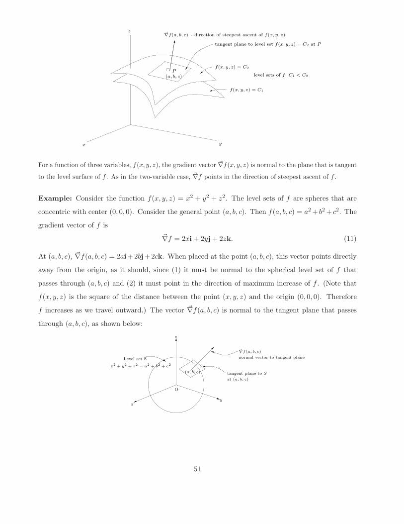
x y

z

level sets of fP

(a, b, c)

f(x, y, z) = C2

f(x, y, z) = C1

tangent plane to level set f(x, y, z) = C2 at P

~∇f(a, b, c) - direction of steepest ascent of f(x, y, z)

C1 < C2

For a function of three variables, f(x, y, z), the gradient vector ~∇f(x, y, z) is normal to the plane that is tangent

to the level surface of f . As in the two-variable case, ~∇f points in the direction of steepest ascent of f .

Example: Consider the function f(x, y, z) = x2 + y2 + z2. The level sets of f are spheres that are

concentric with center (0, 0, 0). Consider the general point (a, b, c). Then f(a, b, c) = a2 + b2 + c2. The

gradient vector of f is

~∇f = 2xi + 2yj + 2zk. (11)

At (a, b, c), ~∇f(a, b, c) = 2ai+2bj+2ck. When placed at the point (a, b, c), this vector points directly

away from the origin, as it should, since (1) it must be normal to the spherical level set of f that

passes through (a, b, c) and (2) it must point in the direction of maximum increase of f . (Note that

f(x, y, z) is the square of the distance between the point (x, y, z) and the origin (0, 0, 0). Therefore

f increases as we travel outward.) The vector ~∇f(a, b, c) is normal to the tangent plane that passes

through (a, b, c), as shown below:

~∇f(a, b, c)

Level set S

x2 + y2 + z2 = a2 + b2 + c2

tangent plane to S

at (a, b, c)

normal vector to tangent plane

xy

z

(a, b, c)

O

51

Exercise: Show that the equation of the tangent plane to the level set of f at (a, b, c) is

ax + by + cz = a2 + b2 + c2. (12)

52

Lecture 8

The gradient and the directional derivative: Conclusion

Example: Consider the following function,

f(x, y, z) =1

(x2 + y2 + z2)1/2=

1

r, (13)

which is of great importance to Physics, as we shall see. The value of f(x, y, z) is simply the distance

from the point (x, y, z) to the origin (0, 0, 0). In contrast to the previous example, the value of f

decreases as we move away from (0, 0, 0). As we approach (0, 0, 0), f increases without bound. The

level sets of r are also spheres that are concentric with center (0, 0, 0). From these observations, we

can already get an idea of how the gradient vectors ~∇f will behave:

1. They must point inward, since f increases as we move inward.

2. They must point directly inward from point P (x, y, z) to the origin (0, 0, 0) because they must

be normal to the spherical level sets.

Let us now perform the calculation of ~∇f :

∂f

∂x=

∂

∂x

[

1

(x2 + y2 + z2)1/2

]

= −x

(x2 + y2 + z2)3/2. (14)

Likewise, we find that∂f

∂y= −

y

(x2 + y2 + z2)3/2, (15)

∂f

∂z= −

z

(x2 + y2 + z2)3/2. (16)

Putting these results together gives

~∇1

(x2 + y2 + z2)1/2= −

1

(x2 + y2 + z2)3/2[xi + yj + zk] (17)

But we may write this in condensed vector form as

~∇1

r= −

1

r3r, (18)

or

~∇1

r= −

1

r2r, (19)

53

where r =‖ r ‖=√

x2 + y2 + z2 and r = r/r is the unit position vector. From this formula, one can

see that the gradient vector behaves in the ways that we predicted earlier.

This is a very important result since the term on the RHS of (18) has the form, up to a constant,

of the “inverse square law” forces we examined earlier: the (electrostatic, gravitational) force field

generated by a point (charge, mass) situated at the origin. If we multiply both sides of Eq. (18) by a

constant K, then

~∇

(

K

r

)

= −K

r3r, (20)

We then have the following two cases:

1. K = GMm: ~∇

(

GMm

r

)

= −GMm

r3r, gravitational field

2. K = −Qq

4πǫ0: ~∇

(

−Qq

4πǫ0r

)

=Qq

4πǫ0r3r, electrostatic field

These force fields are gradient force fields since they can be expressed as the gradients of scalar-

valued functions f which will play the role of potential energy functions, i.e.,

F = ~∇f. (21)

And the level sets of these potential energy functions will be equipotential surfaces.

The term “gradient fields” is employed by mathematicians. In Physics, one usually refers to such

forces as “conservative forces”: A (vector) field F : R3 → R3 is said to be conservative if there exists

a scalar-valued function U : R3 → R such that

F = −~∇U = ~∇(−U). (22)

The appearance of the minus sign “−” in the above equation is convenient from a physical point

of view, as you may already know from your studies of classical mechanics. In any case, we shall

definitely return to this topic later in the course.

54

Chain Rules for multivariable functions

(Relevant section from the textbook by Stewart, Sixth Edition: 14.5)

Suppose that we have a function f : R2 → R that defines some physical quantity of interest, for

example, the temperature at a point (x, y) on a hotplate that is represented by some region D ∈ R2.

Now suppose that x and y are functions of a variable t, i.e. x(t) and y(t). As an example, we suppose

that

r(t) = (x(t), y(t)) (23)

represents the path of of an observer that is moving in the plane and measuring the temperature along

its path. The temperature experienced by the observer at time t will be given by f(x(t), y(t)) which

can be considered a function of t, i.e.,

g(t) = f(x(t), y(t)). (24)

Of course, if we know x(t) and y(t) explicitly, then we could substitute these expressions into that of

f(x, y) to obtain g(t). Mathematically, g : R → R is a composition of the functions f : R2 → R and

r : R → R2, i.e.,

g = f ◦ r.

Example: We return to the ant/hotplate problem studied earlier. The temperature of the hotplate

is given by

f(x, y) = 50 − x2 − 2y2. (25)

This time, the ant is moving: At time t = 0 it starts at the point (0, 5) and moves along the path

r(t) = (x(t), y(t)) = (t, 5 − t2), t ≥ 0, (26)

Then the temperature experienced by the ant is

g(t) = f(x(t), y(t)) = 50 − t2 − 2(5 − t2)2 (27)

= 19t2 − 2t4.

Some level curves of the temperature function f(x, y) along with the path of the ant are sketched

below.

55

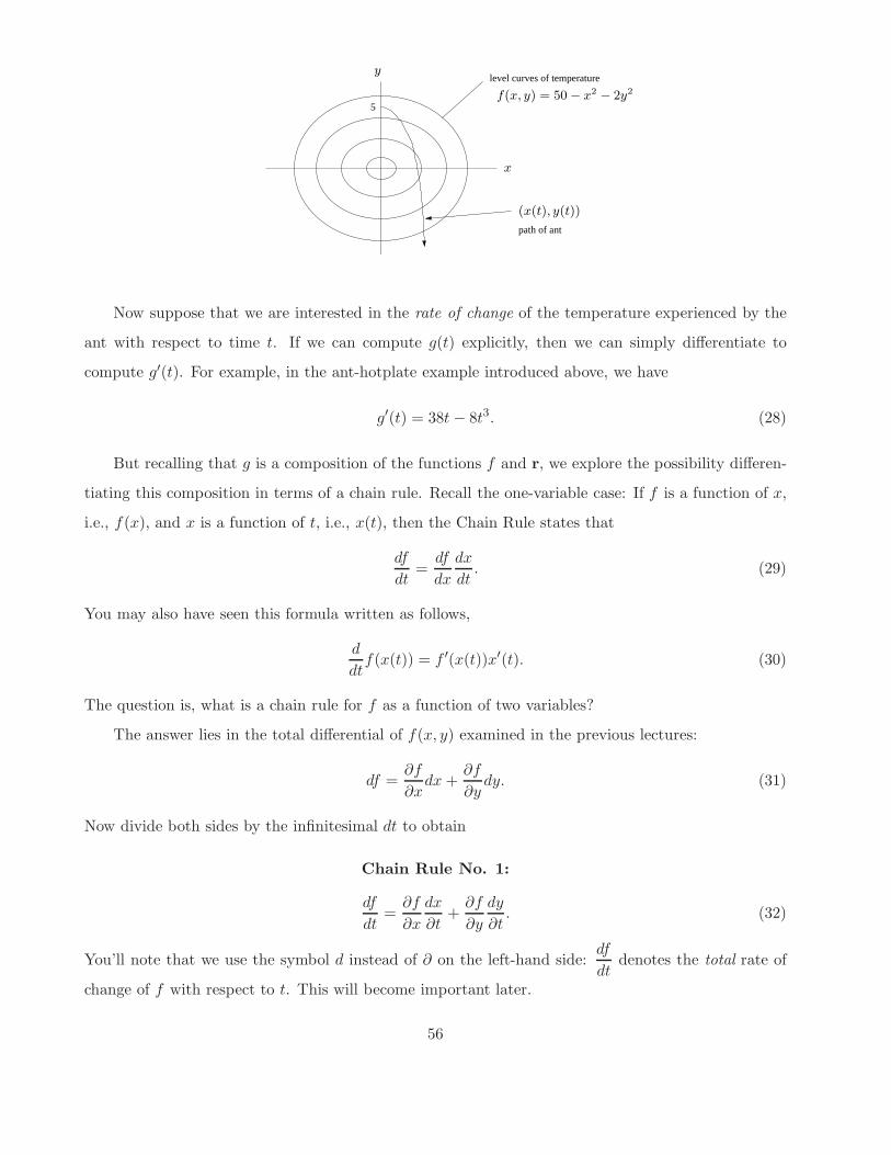
5

level curves of temperature

path of ant

f(x, y) = 50 − x2− 2y2

(x(t), y(t))

x

y

Now suppose that we are interested in the rate of change of the temperature experienced by the

ant with respect to time t. If we can compute g(t) explicitly, then we can simply differentiate to

compute g′(t). For example, in the ant-hotplate example introduced above, we have

g′(t) = 38t − 8t3. (28)

But recalling that g is a composition of the functions f and r, we explore the possibility differen-

tiating this composition in terms of a chain rule. Recall the one-variable case: If f is a function of x,

i.e., f(x), and x is a function of t, i.e., x(t), then the Chain Rule states that

df

dt=

df

dx

dx

dt. (29)

You may also have seen this formula written as follows,

d

dtf(x(t)) = f ′(x(t))x′(t). (30)

The question is, what is a chain rule for f as a function of two variables?

The answer lies in the total differential of f(x, y) examined in the previous lectures:

df =∂f

∂xdx +

∂f

∂ydy. (31)

Now divide both sides by the infinitesimal dt to obtain

Chain Rule No. 1:

df

dt=

∂f

∂x

dx

∂t+

∂f

∂y

dy

∂t. (32)

You’ll note that we use the symbol d instead of ∂ on the left-hand side:df

dtdenotes the total rate of

change of f with respect to t. This will become important later.

56

There is a convenient way to remember this formula in terms of a schematic graph that indicates

the dependencies of variables on other variables. The graphical way to indicate that f is a function

of both x and y and each of x and y are functions of t is as follows:

f

x y

t t

The next step is to determine all paths that lead from f to t as shown below:

f

x y

t t

Path 1 Path 2

The final step, determining the total rate of change of f with respect to t, is done by “summing”

over all paths, i.e., adding up the contributions of each path:

df

dt= Contribution from Path 1 + Contribution from Path 2 (33)

=∂f

∂x

dx

dt+

∂f

∂y

dy

dt.

Let us now compute the rate of change of the temperature experienced by the ant using Chain

Rule No. 1:

df

dt=

∂f

∂x

dx

dt+

∂f

∂y

dy

dt(34)

= (−2x)(1) + (−4y)(−2t)

= (−2t) + (−20 + 4t2)(−2t)

= 38t − 8t3

which agrees with the result obtined earlier by direct substitution.

57

Let us now return to Chain Rule No. 1 and note the the right-hand side is the dot product of two

vectors, namely, the gradient vector,

~∇f =

(

∂f

∂x,∂f

∂y

)

(35)

and the velocity vector r′(t) = v(t) = (x′(t), y′(t)). Thus, Chain Rule No. 1 can be written very

compactly in vector notation asdf

dt= ~∇f · v = ~∇f ·

dr

dt. (36)

This rule is easily generalized to functions of more than two variables. For a function f : R3 → R,

df

dt=

∂f

∂x

dx

∂t+

∂f

∂y

dy

∂t+

∂f

∂z

dz

∂t. (37)

“Chain Rule No. 1(a)”

Recall that if f : R2 → R is a function of two variables x and y that are, in turn, functions of a third

variable, say t, then the result is a composition of functions,

g(t) = f(x(t), y(t)) (38)

For example, g(t) is the temperature experienced by an ant that moves over a hotplate along the path

r(t) = (x(t), y(t)) and the temperature at a point (x, y) on the hotplate is given by f(x, y).

Recall that the rate of change of the temperature experienced by the ant is given by

g′(t) =df

dt=

∂f

∂x

dx

dt+

∂f

∂y

dy

dt, (39)

which we called “Chain Rule No. 1”.

Any change in temperature experienced by the ant is due to its motion and the fact that the

temperature function f(x, y) is not constant over the hotplate. (If f(x, y) = C for all (x, y), then

fx = fy = 0 implies that g′(t) = 0.

But in our treatment so far, we’ve been assuming that the temperature on the hotplate, although

varying from point to point, does not change over time. What happens if the temperature of the

hotplate also changes over time?

In this case, f is a function of three variables, x, y and t, i.e., f(x, y, t). For example, suppose

that the hotplate temperature function is

f(x, y, t) = e−t[50 − x2 − 2y2], t ≥ 0. (40)

58

This represents a hotplate that is cooling in time. As t → ∞, e−t → ∞ which implies that f(x, y, t) → 0

for all points (x, y).

As before, one method of computing the derivative g′(t) is to substitute the expressions for the

path of the ant, i.e.,

x(t) = t, y(t) = 5 − t2, (41)

into the expression for f(x, y, t), i.e.,

g(t) = e−t[50 − t2 − 2(5 − t2)2], (42)

and then differentiate with respect to t. However, what we want to do here is to develop a “chain

rule”-type of differentiation process, as we did for the previous hotplate problem.

Rather than trying to visualize the graph of f(x, y, t), it’s more instructive to examine the graph

of f(x, y, tk) at various fixed times t0 = 0 < t1 < t2 · · ·. At t0 = 0, we have the hotplate function

examined earlier. As t increases, the maximum of the temperature function – in (x, y) space – remains

at (0, 0) but the height of the graph decreases.

x y

z

x y

z z

xy

50

50e−1

50e−2

z = 50 − x2− 2y2

t = 0 t = 1t = 2

z = e−2(50 − x2− 2y2)

z = e−1(50 − x2− 2y2)

Graphs of hotplate temperature function f(x, y, t) = e−t(50 − x2 − 2y2 at three different times. (The hotplate

is cooling.)

The “variable dependency graph” that shows the dependencies of functions on their variables now

becomes

t

f

t t

yx

59

We can now use Chain Rule No. 1 for the function f(x, y, t):

df

dt=

∂f

∂x

dx

dt+

∂f

∂y

dy

dt+

∂f

∂t

dt

dt. (43)

Of course,dt

dt= 1 so that we have simply

df

dt=

∂f

∂x

dx

dt+

∂f

∂y

dy

dt+

∂f

∂t. (44)

We shall refer to this formula as “Chain Rule No. 1(a)” since it still involves differentiation with

respect to a single independent variable, namely, t.

One may well be confused by the appearance ofdf

dton the left-hand side of the expression and

∂f

∂ton the right-hand side. What is the difference between them?

1.df

dtis the rate of change of temperature experienced by the moving ant it moves along the path

(x(t), y(t)) over the hotplate, the temperature of which is given by f(x, y, t).

2.∂f

∂tis, by definition, the rate of change of f while keeping x and y fixed. In other words, it is

the rate of change of the temperature of the hotplate at a fixed point (x, y).

In summary, then: The rate of change of temperature experienced by the ant may be due to two

independent effects:

1. The spatial variation of the hotplate temperature function f(x, y, t) as the ant moves from point

to point,

2. The temporal variation of the hotplate temperature function f(x, y, t) at each point (x, y).

Let us now computedf

dtfor our time-varying hotplate function and the same path of the ant. We

compute the necessary derivatives:

∂f

∂x= −2xe−t,

∂f

∂y= −4ye−t,

∂f

∂t= −e−t[50 − x2 − 2y2], (45)

anddx

dt= 1.

dy

dt− 2t. (46)

60

Thendf

dt= (−2xe−t) + (−4ye−t)(−2t) − e−t(50 − x2 − y2). (47)

We can substitute for x(t) and y(t) to obtain this derivative solely in terms of t. After some algebra

we find thatdf

dt= te−t [38 − 19t − 8t2 + 2t3]. (48)

61

Lecture 9

“Chain Rule No. 2”

(Relevant section from the textbook by Adams and Essex: 14.5)

Now suppose that f is a function of x and y and each of x and y are functions of two variables s

and t. Then f(x(s, t), y(s, t)) defines a function g(s, t), i.e.

g(s, t) = f(x(s, t), y(s, t)). (49)

The graph of variable dependencies is as follows:

t

x y

s t s

f

The question is: How does g, therefore f , change with respect to changes in s and t?

From our earlier work, the differential of g(s, t) is given by

dg =∂g

∂sds +

∂g

∂tdt. (50)

Likewise, the differential of f(x, y) is

df =∂f

∂xdx +

∂f

∂ydy. (51)

And the differentials of x(s, t) and y(x, t) are given by

dx =∂x

∂sds +

∂x

∂tdt (52)

dy =∂y

∂sds +

∂y

∂tdt.

We now substitute (52) into (51):

df =∂f

∂x

[

∂x

∂sds +

∂x

∂tdt

]

+∂f

∂y

[

∂y

∂sds +

∂y

∂tdt

]

(53)

=

[

∂f

∂x

∂x

∂s+

∂f

∂y

∂y

∂s

]

ds +

[

∂f

∂x

∂x

∂t+

∂f

∂y

∂y

∂t

]

dt.

62

If we now consider f as a function of s and t, essentially the function g(s, t) in (49), then (53) can

be considered to be the differential

df =∂f

∂sds +

∂f

∂tdt, (54)

so that we arrive at

Chain Rule No. 2

∂f

∂s=

∂f

∂x

∂x

∂s+

∂f

∂y

∂y

∂s, (55)

∂f

∂t=

∂f

∂x

∂x

∂t+

∂f

∂y

∂y

∂t,

Once again, we can produce these derivatives from the dependency graph given earlier: To obtain, for

example,∂f

∂s, we sum over all paths that extend from f to s.

Example 1: Given f(x, y) = x2y + 2 sin y, where x = st − t and y = s2 +t

s, find

∂f

∂sand

∂f

∂t.

Solution: Using Chain Rule No. 2, we have

∂f

∂s=

∂f

∂x

∂x

∂s+

∂f

∂y

∂y

∂s(56)

= (2xy)(t) + (x2 + 2cos y)(2s −t

s2).

and

∂f

∂t=

∂f

∂x

∂x

∂t+

∂f

∂y

∂y

∂t(57)

= (2xy)(s − 1) + (x2 + 2cos y)(1

s).

We could go one step further and express all x and y in the above expressions in terms of s and t, but

the above results are sufficient.

Example 2: Suppose that

z = f(r, s, x), r = g(x, y), s = h(x, y). (58)

Find∂z

∂xand

∂z

∂y.

63

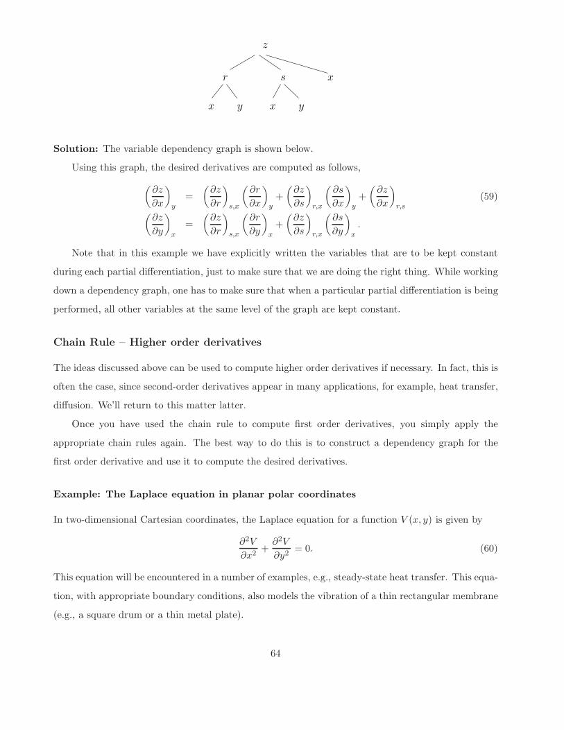
y

z

r s x

x y x

Solution: The variable dependency graph is shown below.

Using this graph, the desired derivatives are computed as follows,

(

∂z

∂x

)

y=

(

∂z

∂r

)

s,x

(

∂r

∂x

)

y+

(

∂z

∂s

)

r,x

(

∂s

∂x

)

y+

(

∂z

∂x

)

r,s(59)

(

∂z

∂y

)

x

=

(

∂z

∂r

)

s,x

(

∂r

∂y

)

x

+

(

∂z

∂s

)

r,x

(

∂s

∂y

)

x

.

Note that in this example we have explicitly written the variables that are to be kept constant

during each partial differentiation, just to make sure that we are doing the right thing. While working

down a dependency graph, one has to make sure that when a particular partial differentiation is being

performed, all other variables at the same level of the graph are kept constant.

Chain Rule – Higher order derivatives

The ideas discussed above can be used to compute higher order derivatives if necessary. In fact, this is

often the case, since second-order derivatives appear in many applications, for example, heat transfer,

diffusion. We’ll return to this matter latter.

Once you have used the chain rule to compute first order derivatives, you simply apply the

appropriate chain rules again. The best way to do this is to construct a dependency graph for the

first order derivative and use it to compute the desired derivatives.

Example: The Laplace equation in planar polar coordinates

In two-dimensional Cartesian coordinates, the Laplace equation for a function V (x, y) is given by

∂2V

∂x2+

∂2V

∂y2= 0. (60)

This equation will be encountered in a number of examples, e.g., steady-state heat transfer. This equa-

tion, with appropriate boundary conditions, also models the vibration of a thin rectangular membrane

(e.g., a square drum or a thin metal plate).

64

Our goal is to rewrite the above Laplace equation in terms of planar polar coordinates r and θ,

i.e., to consider V as a function V (r, θ). Why would we want to do this? Because it is easily to apply

this form of Laplace’s equation to problems that exhibit circular symmetry, for example, the vibration

of a circular membrane, e.g., drum.

Recall that the relationship between the polar coordinates (r, θ) and (x, y) is given by

x = r cos θ, y = r sin θ. (61)

Or, if we express r and θ in terms of x and y:

r =√

x2 + y2, θ = Tan−1(

y

x

)

. (62)

In order to perform the transformation, we are going to want to express the Cartesian derivatives∂2V

∂x2and

∂2V

∂y2in terms of partial derivatives of V with respect to r and θ. We first construct the

appropriate variable dependency graph:

y

V

r θ

x y x

We first calculate the first derivatives using the Chain Rule (or the graph):

∂V

∂x=

∂V

∂r

∂r

∂x+

∂V

∂θ

∂θ

∂x(63)

∂V

∂y=

∂V

∂r

∂r

∂y+

∂V

∂θ

∂θ

∂y

The partials of r and θ w.r.t. x and y are computed from the equations in (62):

∂r

∂x=

x√

x2 + y2=

r cos θ

r= cos θ (64)

and∂θ

∂x=

1

1 +( y

x

)2

(

−y

x2

)

= −y

x2 + y2= −

r sin θ

r2= −

sin θ

r. (65)

Thus∂V

∂x= cos θ

∂V

∂r−

sin θ

r

∂V

∂θ. (66)

In the same way, we compute∂V

∂y= sin θ

∂V

∂r+

cos θ

r

∂V

∂θ. (67)

65

∂V∂x

r θ

x y x y

We’re certainly not finished, however! We must now compute the second derivatives, using the

above dependency graph. From the Chain Rule,

∂2V

∂x2=

∂

∂x

(

∂V

∂x

)

=∂

∂r

(

∂V

∂x

)

∂r

∂x+

∂

∂θ

(

∂V

∂x

)

∂θ

∂x.

=∂

∂r

[

cos θ∂V

∂r−

sin θ

r

∂V

∂θ

]

cos θ +∂

∂θ

[

cos θ∂V

∂r−

sin θ

r

∂V

∂θ

] (

−sin θ

r

)

= cos2 θ∂2V

∂r2+

sin θ cos θ

r2

∂V

∂θ−

sin θ cos θ

r

∂2V

∂r∂θ

+sin2 θ

r

∂V

∂r−

cos θ sin θ

r

∂2V

∂θ∂r+

cos θ sin θ

r2

∂V

∂θ+

sin2 θ

r2

∂2V

∂θ2, (68)

which can be simplified slightly by collecting like terms. A similar calculation gives

∂2V

∂y2= sin2 θ

∂2V

∂r2−

2 sin θ cos θ

r2

∂V

∂θ+

2 sin θ cos θ

r

∂2V

∂r∂θ

+cos2 θ

r

∂V

∂r+

cos2 θ

r2

∂2V

∂θ2. (69)

Substitution of these two results into Laplace’s equation, Eq. (60), yields the following equation,

∂2V

∂r2+

1

r

∂V

∂r+

1

r2

∂2V

∂θ2= 0. (70)

This is Laplace’s equation for V (r, θ) in planar polar coordinates.

One of the motivations for performing this exercise is to show you that the translation of Laplace’s

equation from Cartesian coordinates to another coordinate system is not trivial. In this case, i.e.,

planar Cartesian coordinates to planar polar coordinates, note the appearance of inverse powers of r

multiplying various derivatives of V . This is due to the singularity of the polar coordinate system at

r = 0 – something that we shall discuss later in this course.

66