lecture 6: univariate volatility modelling, arch and...

Lecture 6: Univariate Volatility Modelling, ARCH and GARCH

Prof. Massimo Guidolin

20192– Financial Econometrics

Spring 2017

Overview

2

Stepwise Distribution Modeling Approach Three Key Facts to Remember Volatility Clustering in the Data Naïve Variance Forecast Models: Rolling Window Variance

Estimation and the RiskMetrics System ARCH Models GARCH Models; Comparisons with RiskMetrics Leverage Effects and Component GARCH Estimation of GARCH Models Refinements over GARCH modeling strategies: NGARCH

and other GARCH models Variance Model Evaluation

Lecture 6: Univariate volatility modelling ARCH and GARCH – Prof. Guidolin

Overview and General Ideas

3

Financial economists are concerned with modeling volatility in (individual) asset and portfolio returns because volatility is considered a measure of risk, and investors want a risk premium• As you known, banks and other financial institutions apply so-called

value-at-risk (VaR) models to assess their risks Modeling and forecasting volatility or, in other words, the

covariance structure of asset returns, is therefore important Three steps of a stepwise distribution modeling (SDM) approach:

❶ Establish a variance forecasting model for each of the assets individually and introduce methods for evaluating the performance of these forecasts

❷ Consider ways to model conditionally non-normal aspects of the returns on assets in our portfolio—i.e., aspects that are not captured by conditional means, variances, and covariances

In all finance applications, modeling and forecasting volatility or the covariance structure of asset returns, is crucial


Overview and General Ideas

4

❸ Link individual variance forecasts with a correlation model• The variance and correlation models together will yield a time-

varying covariance model, which can be used to calculate the variance of an aggregate portfolio of assets

The idea that second moments vary over time has an even deeper importance

While most classical finance is built on the assumption that both asset returns and their underlying “fundamentals” are IID Normal over time, casual inspection of GDP, financial aggregates, interest rates, exchange rates etc….

… reveals that these series display time-varying means, variances, and covariances• Fundamentals = quantities that justify asset prices in a rational

framework

Most time series of asset returns, bond yields and exchange rates exhibit time-varying means, variances, and covariances


Three Key Results to Bear in Mind

5

When variances and covariances are time-varying we speak about conditional HETEROSKEDASTICITY

3 simple facts to remember and understand:

• Even though the variance may go through high and low periods, the unconditional (long-run, steady-state, average) variance may exist and be actually constant

• E.g., consider the (dividend-corrected) realized returns on a value-weighted index (by CRSP) of NYSE, AMEX, and NASDAQ stocksLecture 6: Univariate volatility modelling ARCH and GARCH – Prof. Guidolin

① The fact that the conditional variance may change in heteroskedastic fashion, does not necessarily mean the series is non-stationary

② Conditional heteroskedasticity implies that the unconditional, long-run distribution of asset returns will be non-normal

③ Many models of conditional heteroskedasticity, but in the end we care for their forecasting performance

Volatility Clustering in the Data

6

• Sample period is 1972:01-2009:12, monthly data

Our objective is to develop models that can fit the sequence of calm and turbulent periods…

… and especially forecast them• Note: value-weighted NYSE/AMEX/NASDAQ are ptf. returns!


For most (all?) financial time series, volatility “clusters”: high (low) volatility tends to be followed by high (low) volatility

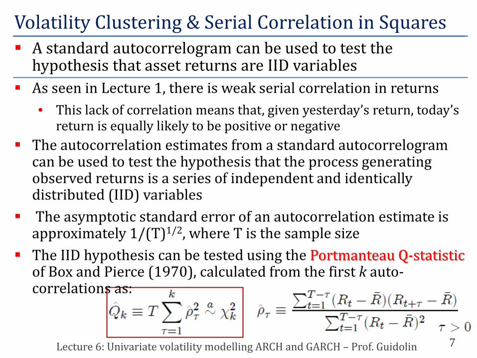
As seen in Lecture 1, there is weak serial correlation in returns• This lack of correlation means that, given yesterday’s return, today’s

return is equally likely to be positive or negative The autocorrelation estimates from a standard autocorrelogram

can be used to test the hypothesis that the process generating observed returns is a series of independent and identically distributed (IID) variables

The asymptotic standard error of an autocorrelation estimate is approximately 1/(T)1/2, where T is the sample size

The IID hypothesis can be tested using the Portmanteau Q-statisticof Box and Pierce (1970), calculated from the first k auto-correlations as:

Volatility Clustering & Serial Correlation in Squares

7Lecture 6: Univariate volatility modelling ARCH and GARCH – Prof. Guidolin

A standard autocorrelogram can be used to test the hypothesis that asset returns are IID variables

The asymptotic distribution of the Qk statistic, under the null of an IID process, is Chi-square, with k degrees of freedom

VW CRSP Stock Returns 10 Year U.S. Govt. Bond Returns

Does this mean that stock & bond returns are (approximately) IID? Unfortunately not: it turns out that the squares and absolute values

of stock and bond returns display high and significant autocorrelations



A standard autocorrelogram can be used to test the hypothesis that asset returns are IID variables

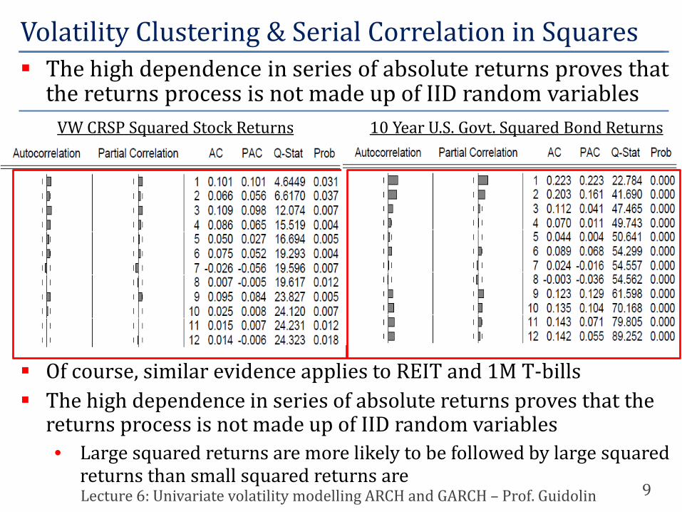
VW CRSP Squared Stock Returns 10 Year U.S. Govt. Squared Bond Returns

Of course, similar evidence applies to REIT and 1M T-bills The high dependence in series of absolute returns proves that the

returns process is not made up of IID random variables• Large squared returns are more likely to be followed by large squared

returns than small squared returns are



The high dependence in series of absolute returns proves that the returns process is not made up of IID random variables

Here the conceptual point is that while

the opposite does not hold: How to explain this phenomenon? If changes in price volatility create clusters of high and low

volatility, this may reflect changes in the flow of relevant information to the market • These stylized facts can be explained by assuming that volatility

follows a stochastic process where today’s volatility is positively correlated with the volatility on any future day

This is what ARCH and GARCH models are for, but first we introduce a few alternatives that historically were developed before ARCH and GARCH were



The high dependence in series of absolute/squared returns proves that the return process is not IID

Consider the simple model for one asset (or ptf.) return:

Here Rt+1 is the continuously compounded return and zt+1 is a pure “shock” to returns, zt+1 = Rt+1/t+1

The model assumes (as in Christoffersen’s book) that the mean = 0 This is an acceptable approximation on daily data; absent this

assumption, the model is Rt+1 = + t+1zt+1

The assumption of normality will be discussed/removed in lecture 6 The easiest way to capture volatility clustering is by letting

tomorrow’s variance be the simple average of the most recent m observations, as in

Naïve Models: Rolling Window Forecasts


In a rolling window variance model the forecast of time t+1 variance is a moving average of m recent squared returns

Constant weighting

However, the fact that the model puts equal weights (equal to 1/m) on the past m observations yields unwarranted results

When plotted over time, variance exhibits box-shaped patterns • An extreme return (positive or negative) today will bump up variance

by 1/m times the return squared for exactly m periods after which variance immediately will drop back down

The autocorrelation plotof squared returns sug-gests that a more gradualdecline is warranted in the effect of past returns on today’s variance

Also: how shall we pick m?

Naïve Models: Rolling Window Forecasts


A high m will lead to an excessively smoothly evolving t+1, and a low m will lead to an excessively jagged pattern of t+1

A more interesting model is JP Morgan’s RiskMetrics system:

The weights on past squared returns decline exponentially as we move backward in time: 1, , 2, …

Also called the exponential variance smoother Because for = 1 we have 0 = 1, it is possible to re-write it as:

which is equivalent to: See lecture notes for why this is the case A weighted avg. of today’s variance and today’s squared return

Naïve Models: RiskMetrics


In JP Morgan’s RiskMetrics model the forecast of variance is a weighted avg. of today’s variance and today’s squared return

The key advantages of the RiskMetrics model are:❶ Recent returns matter more for tomorrow’s variance than

distant returns do as is less than 1 and therefore gets smaller when the lag, , gets bigger

❷ It only contains one unknown parameter, • When estimating on a large number of assets, RiskMetrics found

that the estimates were quite similar across assets, and therefore simply set = 0.94 for every asset for daily data

• In this case, no estimation is necessary❸ Little data need to be stored in order to calculate

tomorrow’s variance; in fact, after including 100 lags of squared returns, the cumulated weight is already close to 100%

Of course, once R2t, is calculated, past returns are not needed

Given all these advantages of the RiskMetrics model, why not simply end the discussion on variance forecasting here?



• The RiskMetrics model has a number of shortcomings, but these can be understood only after introducing ARCH models

• Historically, ARCH models were the first-line alternative developed to compete with exponential smoothers

In the zero-mean return case, their structure is very simple:

This is a ARCH(1) However, historically it was soon obvious that just using one lag of

past squared returns would not be sufficient One needs to use a large number q > 1 of lags on the RHS This means that squared returns are best modeled using an AR(q)

instead of a simple AR(1)• Yet ARCH(1) already implies one complication: they require nonlinear

parameter estimation

ARCH Models


In a ARCH(q) model the forecasts of variance depends on q lags of squared returns, 2

t+1 = + 1R2t + 2R2

t-1 +… + qR2t-q+1

But from the first part of this course, you know already where to look for: ARMA models

The simplest generalized autoregressive conditional heteroskedasticity (GARCH(1,1)) model is:

The implied, unconditional, or long-run average, variance, 2, is

This derives from

Furthermore, if one solves for from the long-run variance expression and substitutes it into the GARCH equation:

Generalized ARCH (GARCH) Models


In a GARCH(1,1) the forecast of variance depends on one lag of squared returns and on past variance, 2

t+1 = + R2t + 2

t

, α > 0, β > 0

Therefore a GARCH(1,1) implies that tomorrow’s variance is a weighted average of the long-run variance, today’s squared return, and today’s variance

Or, tomorrow’s variance is predicted to be the long-run average variance with:• something added (subtracted) if today’s squared return is above

(below) its long-run average, and • something added (subtracted) if today’s variance is above (below)

its long-run average How do you forecast variance in a GARCH model? The one-day forecast of variance, 2

t+1|t, is given directly by the model as 2

t+1; as for multi-periods forecasts, one can show that:

GARCH Models: Forecasting


Long-run forecasts in a GARCH(1,1) are a function of the persistence ( + ) and of initial deviations from steady-state

This implies that as the forecast horizon H grows, because for (+) < 1 implies that ( + )H-1 → 0, then Et[2

t+H] → 2

• For shorter horizons instead, Et[2t+H] > 2 when 2

t+1 > 2 and vice-versa when 2

t+1 < 2

• The conditional expectation, Et[⋅], refers to taking the expectation using all the information available at the end of day t, which includes the squared return on day t itself

(+) plays a crucial role and it is commonly called the persistence level/index of the model

A high persistence, (+) close to 1, implies that shocks which push variance away from its long-run average will persist for a long time

Of course, eventually the long-horizon forecast will be the long-run average variance, 2

In asset allocation problems, we sometimes care for the variance of long-horizon returns,



As we assume that returns have zero autocorrelation (from their sample stats), the variance of the cumulative H-day returns is:

Solving in the GARCH(1,1) case, we have:

• You will see in a moment why establishing a difference w.r.t. H2t+1 is

so important… Let’s now compare GARCH(1,1) and RiskMetrics: are they so

different? In a way they are not: comparing with

you can see that RiskMetrics is just a aspecial case of GARCH(1,1)



The variance of cumulative, H-period returns is not simply H times the long run variance of each return

A RiskMetrics model is a special case in which = 0 and = = 1 – so that, equivalently, + = 1; this has a number of implications:

Implication 1: because = 0 and + = 1, under RiskMetrics the long-run variance does not exist as gives an indeterminate ratio “0/0”• While RiskMetrics ignores that long-run average variance tends to be

relatively stable over time, a GARCH model with ( + ) < 1 does not Equivalently, while a GARCH with ( + ) < 1 is a stationary process,

a RiskMetrics model is not Implication 2: because , under

RiskMetrics + = 1, so that

which means that any shock to current variance is destined to persist forever

GARCH Models: Comparison with RiskMetrics


A JPM RiskMetrics(1,1) model is just a special, restricted, non-stationary case of GARCH(1,1)

∀H

• If today is a high-variance day, then the RiskMetrics model predicts that all future days will be high-variance

• A GARCH more realistically assumes that eventually in the future variance will revert to the average value

Implication 3: Under RiskMetrics, the variance of long-horizon returns is:

What is the density, thedistribution of long-hori-zon returns implied bythese models? Impossibleto show in closed form,see the posted lecture notes

GARCH Models: Comparison with RiskMetrics

23Lecture 6: Univariate volatility

In a JPM RiskMetrics(1,1) model long-run variance does not exist (it explodes), any shock to current variance persists forever, and the variance of long-horizon returns is H2

t+1

α = 0.05, β = 0.90, σ2 = 0.00014

RiskMetrics

GARCH(1,1)

t+H /H

A number of papers have emphasized that a negative return increa-ses variance by more than a positive return of the same magnitude• This may be because, in the case of stocks, as a negative return on a

stock implies a drop in the equity value, which implies that the company becomes more highly levered and thus riskier (assuming the level of debt stays constant)

We can modify GARCH models so that the weight given to the return depends on whether the return is positive or negative

This is described by the (sample) news impact curve (NIC) The NIC measures how new information is incorporated into

volatility, i.e. it shows the relationship between the current return Rt and conditional variance one period ahead 2

t+1, holding constant all other past and current information

GARCH Models with Leverage


According to the leverage (asymmetric variance) effect, a negative return increases variance by more than a positive return of the same magnitude

In a GARCH(1,1) model we have:NIC(Rt|2

t+1 = 2) = + R2t + 2

= A + R2t

which is a quadratic function of R2t

and therefore symmetric around 0 (with intercept A + 2 )

Problem: for most return series, the empirical NIC fails to be symmetric

EGARCH is probably the most prominent asymmetric GARCH• As in ARCH models, in GARCH models the negativity of parameters

may create difficulties in estimation• Nelson (1991) has proposed a new form of GARCH, the Exponential

GARCH (EGARCH), in which positivity of the conditional variance is ensured by the fact that ln(2

t+1) is directly modeled

GARCH Models with Leverage: EGARCH


The news impact curve describes the relationship between the current return Rt and conditional variance 2

t+1

GARCH

Asymmetric NIC

Two types of EGARCH(1,1) found in the applied literature; the first type is the one originally proposed by Nelson

Letting zt [Rt/t], the log-conditional variance is:

The sequence g(zt) is a zero-mean, i.i.d. random sequence:• If zt > 0, g(zt) is linear in zt with slope + 1

• If zt < 0, g(zt) is linear in zt with slope - 1

Thus, g(zt) is function of both the magnitude and the sign of zt and it allows the conditional variance process to respond asymmetrically to rises and falls in stock prices

Can be rewritten as

GARCH Models with Leverage: EGARCH


An EGARCH model features both asymmetries and non-linearities and it avoids constrained ML estimation

R

tt

The term represents a magnitude effect: If 1 > 0 and = 0, the innovations in the conditional variance are

positive (negative) when the magnitude of zt is larger (smaller) than its expected value

If 1 = 0 and < 0, the innovation in conditional variance is positive (negative) when returns innovations are negative (positive), in accordance with empirical evidence for stock returns

Another way of capturing the leverage effect is to define an indicator variable, It , to take on the value 1 if day t return is negative and zero otherwise

The variance dynamics can now be specified as

Equivalent to have 2

t+1 = + (1 + )R2t + 2

t after negative returns and 2

t+1 = + R2t + 2

t after positive ones

GARCH Models with Leverage


A positive θ will again capture the leverage effect This model is sometimes referred to as the GJR-GARCH model or

threshold GARCH (TARCH) model• GJR = Glosten, Jagannathan, and Runkle

In this model, because when 50% of the shocks will be negative and the other 50% positive, long run variance is [ /(1 - (1 + 0.5θ) - )]; the persistence index is [(1 + 0.5θ) + ]

There is also a smaller literature that has connected time-varying volatility not to time series features, but to observable economic phenomena, especially at daily frequencies• For instance, days where no trading takes place–days that follow a

weekend or a holiday have higher variance:

where IT=1 in correspondence to a day that follows a weekend

GARCH Models with Leverage: Threshold GARCH


In a TARCH model the reaction to shocks is captured by a step-wise linear fnct. that differs for positive vs. negative shocks

• Other predetermined variables could be yesterday’s trading volume or prescheduled news announcement dates such as company earnings and FOMC meetings dates

• Option implied volatilities have quite a high predictive value in forecasting next-day variance, e.g., the CBOE VIX (squared)

In general, such models that use explanatory variables to capture time-variation in variance are represented as:

where Xt are predetermined variables Important to ensure that the GARCH model always generates a

positive variance forecast You need to ensure that , , , and g(Xt) are all positive How do you estimate a GARCH model? This means, how do you estimated the fixed but unknown

parameters , , and ?

GARCH Models with Predetermined Variables


To perform point estimation, you need to propose one estimator (or method of estimation) with “good” properties

For GARCH, maximum likelihood (MLE) is such method The method is simply based on knowledge of the likelihood

function, which is affine to the joint probability density function (PDF) of all of your data

Because the assumption of IID normal shocks (zt) implies that the density of the time t observation is:

Because each shock is independent of the others, the total probability (PDF) of the entire sample is then the product of T such densities:

Maximum Likelihood Estimation


GARCH models are estimated by maximum likelihood on the basis of a Gaussian assumption for shocks to returns

This is also called the likelihood function; however, because it is more convenient to work with sums than with products, we usually consider the log of the likelihood function,

also called log-likelihood function The idea is the the log-lik (its nickname) depends on the unknown

parameters in a (say) GARCH (1,1), 2t = + R2

t-1 + 2t-1

Therefore we shall simply maximize such log-lik to select the unknown parameters: “maximize” + “the log-lik” MLE

How do you do it, with paper and pencil? In the case of GARCH, no, you need to perform numerical constrained optimization

• What? That’s why we shall need Eviews or Matlab (or Excel?!)…



• Note: you need to estimate imposing constraints on the parameters to keep variance positive and the process stationary

• Need to impose > 0, 0, 0, and (+ ) < 1 MLEs have very strong theoretical properties: They are consistent estimators: this means that as the sample size T ∞, the probability that the value of the estimators (in repeated samples) shows a large divergence from the true (unfortunately unknown) parameter values, goes to 0 They are the most efficient estimators (i.e., those that give estimates with the smallest standard errors, in repeated samples) among all the (asymptotically) unbiased estimators• Please also see posted Stat prep course notes for details• What is asymptotically unbiased? Something related to consistent

(not exactly the same, but the same for most cases)



Under regularity conditions, MLEs are consistent, asym-ptotically normal, and minimum variance estimators

Something to note: MLE requires knowledge of Who told you that this is actually the case? What if, with your data,

this is probably NOT the case? Can we still somehow do what we described above and enjoy some of the good properties of MLE?

Answer: Yes – it is called quasi (or pseudo) maximum likelihood estimation (QMLE)

Key result: even if the conditional distribution of the shocks zt is not normal, MLE will yield estimates of the mean and variance parameters, which converge to the true parameters as the sample gets infinitely large… …. as long as the mean and variance fncts are correctly specified

“Correctly specified” = the models for conditional mean and variance functions are “right” (in a statistical sense)

Quasi-Maximum Likelihood Estimation (QMLE)


Consistent QML estimators are obtained incorrectly assuming a normal distribution, if the conditional mean and variance functions are correctly specified

In short, the QMLE result says: you can still use MLE estimation even when the shocks are not normally distributed if your choices of conditional mean and variance function are good zt will have to be anyway IID; you can just do without normality Conditional mean function = how t depends on past information in

more general model is Rt+1 = t+1 + t+1zt+1

Conditional variance fnct: GARCH(p,q), TARCH(p,q), RiskMetrics, etc. In practice, QMLE buys us the freedom to worry about the

conditional distribution later on, and we will Too good to be true: what is the true cost of QMLE? Simple, QMLEs

will in general be less efficient than those from MLE We trade-off theoretical asymptotic efficiency and practicality

QMLE comes in handy also when holds: when we shall need to “split-up” estimation in different stages



QML estimators are less efficient than ML estimators

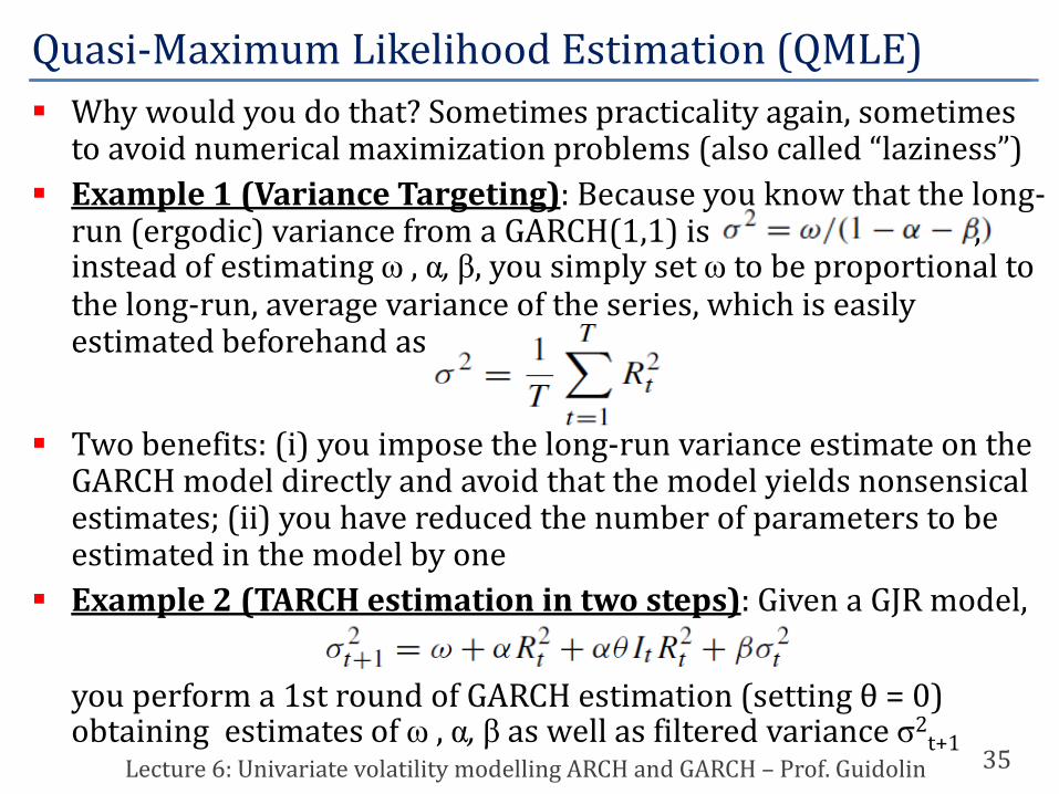
Why would you do that? Sometimes practicality again, sometimes to avoid numerical maximization problems (also called “laziness”)

Example 1 (Variance Targeting): Because you know that the long-run (ergodic) variance from a GARCH(1,1) is , instead of estimating , , , you simply set to be proportional to the long-run, average variance of the series, which is easily estimated beforehand as

Two benefits: (i) you impose the long-run variance estimate on the GARCH model directly and avoid that the model yields nonsensical estimates; (ii) you have reduced the number of parameters to be estimated in the model by one

Example 2 (TARCH estimation in two steps): Given a GJR model,

you perform a 1st round of GARCH estimation (setting θ = 0) obtaining estimates of , , as well as filtered variance 2

t+1



• Call these estimates *, *, and *• Next you regress (2

t+1 - *) on (i) *R2t, (ii) *It R2

t, and (iii) *2t to

obtain an estimate of θ, call it θ*• You keep iterating on this process until convergence

Of course nobody would really do that, but the point is: even these estimates, because they are not obtained in one single-pass using all the available information, will be QMLE estimates

Three dimensions in which simple (“plain vanilla”) GARCH may be generalizedWriting general NICs as part of the model specification• Recall: NIC measures the reaction of 2

t+1 to standardized shocks zt

• E.g., in GARCH(1,1) case, NIC(zt) = 2t z2

t (because R2t = 2

t z2t)



Two-step, seemingly ML estimation can be seen as a QMLE GARCH models can be generalized by extending the NIC to

incorporate new and specific features

There is a family of volatility models parameterized by 1, 2, 3

NIF(zt) = [|zt – 1| - θ2(zt – θ1)]2θ3

• How do you retrieve a standard GARCH?• In principle, the “game” is now to estimate 1, 2, and 3 from the data

Yet one simple choice (2 = 0, 3 = 1) is rather famous: the Nonlinear (asymmetric) GARCH, or N(A)GARCH

σ2t+1 = + (Rt - σt)2 + σ2

t = + σ2t(zt - )2 + σ2

t

• NGARCH plays key role in option pricing with stochastic volatility• Last topic in syllabus: under some conditions get closed formulas

The model is asymmetric when > 0 because while zt 0 impacts conditional variance only in the measure (zt - )2 z2

t, zt < 0 impacts conditional variance in the measure (zt - )2 > z2

t

Generalizing GARCH Models: N(A)GARCH


A Nonlinear (asymmetric) GARCH follows the process σ2t+1 =

+ (Rt - σt)2 + σ2t

The model is non-linear because even under = 0 it can be re-written as a GARCH(1,1) in zt with time-varying ARCH coefficient:

σ2t+1 = + tz2

t+ σ2t = + ( + z2

t)σ2t where t σ2

t

• Models in which the coefficients are not constant, but are a function of time (or variables that change over time) are non-linear models

• The NGARCH persistence is given by (1 + 2) + • With some algebra (see lecture notes) you can show that the

unconditional variance is /(1 – (1+2) – )We have focused on simple GARCH(1,1) models as they are easy to interpret and they usually work (in particular, the NGARCH did)

In some applications (although rare), generalized (p, q) GARCH models appear:

Generalizing GARCH Models


GARCH models may be easily generalized to include p ARCH lags and q generalized lags of past variance

• Very few data sets seem to require them and in any event I never saw a model bigger than a GARCH(2,2)

• The real problem is estimation, as many constraints have to be imposed to ensure that variance is positive

• Conditions for stationarity are also rather complexModels that distinguish between the dynamics in short- vs. long-term variance, also called Component GARCH models

The intuition is simple: in a stationary GARCH(1,1) model, short-term variance is time-varying, but long-run variance is a constant, σ2 = ω/(1 -α - β)

In a component GARCH model: (i) short-run variance is time-varying and follows a GARCH(1,1); (ii) also long-run variance is time-varying and follows a GARCH(1,1)

Generalizing GARCH Models: Component GARCH


In a component GARCH models there are two different layers: short-run variance is time-varying and follows a GARCH; long-run variance is time-varying and follows a GARCH

• Here σ2t is (as usual) short-run variance; vt is long-run variance

Good model because it captures the slow decay of auto-correlations in squared returns that we found in lecture 1

Your lecture notes showthat a component GARCHcan be re-written as re-stricted GARCH(2,2) models

The slow decay of the auto-correlation function in the case of daily S&P 500 stock returns

Generalizing GARCH Models: Component GARCH


A component GARCH(1,1) model can always be re-written as restricted, plain vanilla GARCH(2,2) models

Short-run GARCH(1,1)Long-run GARCH(1,1)

Long-run GARCH(1,1)

Let’s now move where the money is (or not): how can you tell whether a (univariate) volatility model works in practice?

A number of techniques – called diagnostic checks – exist: here we just discuss 3 among the many possible methods

① (Normality tests) If you have estimated by MLE and exploited the assumption that , then the standardized model residuals defined as zt = Rt/σt should have a normal distribution

Use a Jarque and Bera test: JB proposed a test that measures departure from normality in terms of the skewness and kurtosis

Under the null hypothesis of normally distributed errors, the JB statistic has a known asymptotic distribution:

Variance Model Evaluation


Normality of standardized residuals derived from a volatility model may be assessed from JB statistic which is based on deviations of sample skewness and kurtosis from 0 and 3

Zero under N(0,1)

Zero under N(0,1)

Large values of this statistic indicate departures from normality; see also next lecture② (Squared Autocorrelation Tests) Even though normality has not been assumed (QMLE), a good model implies that the squared standardized residuals, z2

t = R2t/σ2

t, should display no systematic autocorrelation patterns• Whether this has been achieved can be assessed in standard

autocorrelation plots that you have seen before• Standard errors are calculated simply as 1/(T1/2), where T is the

number of observations in the sample• So-called Bartlett standard error bands give the range in which the

autocorrelations would fall roughly 95% of the time if the true but unknown autocorrelations were all zero

• In the example , there is little or no serial correlation in the levels of zt, but there is some serial correlation left in the squares, at low orders



If the volatility model is correctly specified, then standardized squared residuals should be uncorrelated

• Probably this means that one should build a different/bettervolatility model

③ (Variance Regressions) The idea is simply to regress squaredreturns computed over a forecast period on the forecast from the variance model:



If the volatility model is correctly specified, then standardized squared residuals should be uncorrelated

Levels Squares

A good variance forecast model should be unbiased, that is, have an intercept b0 = 0, and be efficient, that is have a slope, b1 = 1

Problem: In this regression, the squared returns is used as a proxy for the true but unobserved variance in period t+1; how good of a proxy is the squared return? On the one hand, in principle we are fine because

and from our model Rt+1 = σt+1zt+1

On the other hand, the variance of such a proxy may be poor:

• Because tends much higher than 3 in reality, the variance of the square proxy for realized variance is often very poor (i.e., imprecisely estimated)



If the volatility model is correctly specified, in a variance regression model , b0 = 0 and b1 = 1

Kurtosis coefficient

Due to the high degree of noise in the squared returns, the fit of the preceding regression as measured by the regression R2 will be very low, typically around 5 to 10%, even if the variance model used to forecast is indeed the correct one

Thus obtaining a low R2 in such regressions should not lead one to reject the variance model

However it remains true that the null hypothesis of b0 = 0 and b1 = 1 should not be rejected, if the volatility model is any good

Stay tuned, in lecture 7 we will examine alternative and much better measures of realized variance



If the volatility model is correctly specified, in a variance regression model , b0 = 0 and b1 = 1

Carefully read these Lecture Slides + class notes

Possibly read BROOKS, chapter 9 (sections 1-20).

Possibly read CHRISTOFFERSEN, chapter 4 (sections 1-20).

Lecture Notes are available on Prof. Guidolin’s personal web page

Andersen, T., T. Bollerslev, P. Christoffersen, and F. Diebold (2006) “Volatility and Correlation Forecasting”, in Elliott G., C. Granger, and A. Timmermann (eds.), Handbook of Economic Forecasting, Elsevier.

Engle, R. F. (2001) “GARCH 101: The Use of ARCH/GARCH Models in Applied Econometrics”, Journal of Economic Perspectives, 15, 157-168.

Reading List/How to prepare the exam

46Lecture 5: Cointegration and Error Correction Models – Prof. Guidolin

Appendix A: Forecasting with GARCH(1,1)

47Lecture 3: Multivariate Time Series Analysis– Prof. Guidolin

In the lecture, we have stated that

This comes from the fact that:

and this yields

lecture 6: univariate volatility modelling, arch and...

Documents