lecture 6: umvues and the cramér-rao lower bound

Lecture 6: UMVUEs and the Cramer-Rao LowerBound

MATH 667-01Statistical Inference

University of Louisville

September 17, 2019Last modified: 9/19/2019

1 / 22 Lecture 6: UMVUEs and the Cramer-Rao Lower Bound

Introduction

We start by discussing uniform minimum variance unbiasedestimators1.

We then review correlation2.

We discuss and prove the Cramer-Rao Inequality and somecorollaries3.

1CB: Section 7.3, HMC: Section 7.12CB: Section 4.5, HMC: Section 2.53CB: Section 7.3, HMC: Section 6.2


Best Unbiased Estimator (UMVUE)

In this lecture, we evaluate an estimator W of a parameter θbased on the squared error loss function.

If we consider only unbiased estimators, thenEθ[(W − θ)2] = Varθ[W ].

Definition L6.1:4 An estimator W ∗ is a best unbiasedestimator of τ(θ) if it satisfies Eθ[W

∗] = τ(θ) for all θ and,for any other unbiased estimator W with Eθ[W ] = τ(θ), wehave Varθ[W

∗] ≤ Varθ[W ] for all θ.

W ∗ is also called a uniform minimum variance unbiasedestimator (UMVUE) of τ(θ).

4CB: Definition 7.3.7 on p.334; HMC: Definition 7.1.1 on p.4133 / 22 Lecture 6: UMVUEs and the Cramer-Rao Lower Bound


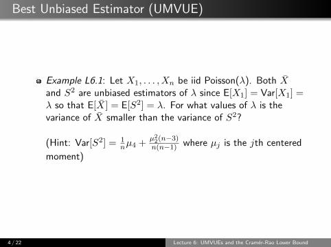
Example L6.1: Let X1, . . . , Xn be iid Poisson(λ). Both Xand S2 are unbiased estimators of λ since E[X1] = Var[X1] =λ so that E[X] = E[S2] = λ. For what values of λ is thevariance of X smaller than the variance of S2?

(Hint: Var[S2] = 1nµ4 +

µ22(n−3)n(n−1) where µj is the jth centered

moment)



Answer to Example L6.1: We know Var[X]3.20=

Var[X1]

n=λ

n.

We can compute E[X] = λ, E[X2] = λ2 + λ,E[X3] = λ2 + 3λ2 + λ, and E[X4] = λ4 + 6λ3 + 7λ2 + λ.

So, we have

E[(X − µ)4] = E[X4]− 4E[X3]µ+ 6E[X2]µ2 − 4E[X]µ3 + µ4

= E[X4]− 4E[X3]µ+ 6E[X2]µ2 − 3µ4

= 3λ2 + λ.

Using the hint, we see that

Var[S2] =1

n(3λ2 + λ)− λ2(n− 3)

n(n− 1)

=1

n

[λ+

2n

n− 1λ2

]so Var[X] < Var[S2] for all λ.


Regularity Assumptions

Let X1, . . . , Xn be a random sample with common pdf f(x; θ) and cdf F (x; θ) forθ ∈ Θ and let W (x) = W (x1, . . . , xn) be a function. Here are some regularityassumptions5 that will be used for several upcoming theorems.

(R0) The cdfs are distinct.

(R1) The pdfs have common support for all θ.

(R2) The true parameter value θ0 is an interior point of Θ.

(R3) The pdf f(x; θ) is twice differentiable as a function of θ.

(R4) The integral∫f(x; θ) dx can be differentiated twice under the integral sign as a

function of θ.

(R5) The integral∫w(x)f(x; θ) dx can be differentiated under the integral sign as a

function of θ.

(R6) The pdf f(x; θ) is three times differentiable as a function of θ, and for allθ ∈ Θ, there exist c ∈ R and a function M(x) such that∣∣∣∣ ∂3∂θ3 ln f(x; θ)

∣∣∣∣ ≤M(x),

with Eθ0 |M(X)| <∞, for all θ0− c < θ < θ0 + c and all x in the support of X.

5slightly different conditions in HMC: p.356+362+368 and CB: p.5166 / 22 Lecture 6: UMVUEs and the Cramer-Rao Lower Bound

Cramer-Rao Lower Bound

Theorem L6.1:6 If X is a random variable with pdf f(x; θ)which satisfies regularity assumptions (R1), (R3), and (R4),then

E

[∂

∂θln f(X; θ)

]= 0

and

Eθ

[(∂

∂θln f(X; θ)

)2]

= −Eθ

[∂2

∂θ2ln f(X; θ)

].

The quantity I(θ) = Eθ

[(∂

∂θln f(X; θ)

)2]

is called the

information number or Fisher information.

6CB: Lemma 7.3.11 on p.338, HMC: page 3637 / 22 Lecture 6: UMVUEs and the Cramer-Rao Lower Bound


Proof of Theorem L6.1: First, we see that

E

[∂

∂θln f(X; θ)

]=

∫ {∂

∂θln f(x; θ)

}f(x; θ) dx

=

∫ ∂∂θf(x; θ)

f(x; θ)f(x; θ) dx

=

∫∂

∂θf(x; θ) dx

=d

dθ

∫f(x; θ) dx =

d

dθ1 = 0.



Proof of Theorem L6.1 continued: Note that

∂2

∂θ2[ln f(x; θ)] =

∂

∂θ

{∂∂θf(x; θ)

f(x; θ)

}

=∂2

∂θ2f(x; θ)

f(x; θ)−(∂∂θf(x; θ)

)2(f(x; θ))2

.

Then, we have

E

[∂2

∂θ2f(X;θ)

f(X; θ)

]=

∫∂2

∂θ2f(x; θ) dx

=

∫∂

∂θ

{∂

∂θf(x; θ)

}dx



Proof of Theorem L6.1 continued:

=

∫∂

∂θ

{∂

∂θf(x; θ)

}dx

=

∫∂

∂θ

{∂∂θf(x; θ)

f(x; θ)f(x; θ)

}dx

=

∫∂

∂θ

{(∂

∂θln f(x; θ)

)f(x; θ)

}dx

=d

dθ

∫ {(∂

∂θln f(x; θ)

)f(x; θ)

}dx

=d

dθ

∫ { ∂∂θf(x; θ)

f(x; θ)f(x; θ)

}dx

=d

dθ

∫∂

∂θf(x; θ) dx =

d

dθ

{d

dθ

∫f(x; θ) dx

}=

d

dθ[1] = 0



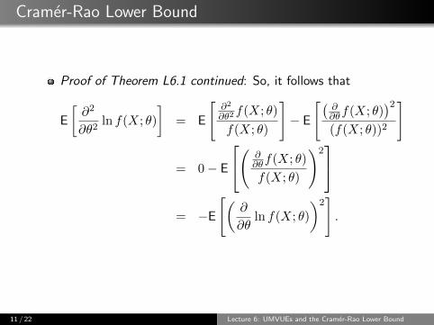
Proof of Theorem L6.1 continued: So, it follows that

E

[∂2

∂θ2ln f(X; θ)

]= E

[∂2

∂θ2f(X; θ)

f(X; θ)

]− E

[(∂∂θf(X; θ)

)2(f(X; θ))2

]

= 0− E

( ∂∂θf(X; θ)

f(X; θ)

)2

= −E

[(∂

∂θln f(X; θ)

)2].


Review: Correlation

E[X] = µX , E[Y ] = µY , Var[X] = σ2X , Var[Y ] = σ2

Y

Assume 0 < σ2X <∞ and 0 < σ2

Y <∞Definition L6.2:7 The correlation of X and Y is the numberdefined by

ρXY =Cov[X,Y ]

σXσY.

The value ρXY is also called the correlation coefficient.

Theorem L6.2:8 For any random variables X and Y ,

(a) −1 ≤ ρXY ≤ 1.(b) |ρXY | = 1 if and only if there exists numbers a 6= 0 and b such

that P (Y = aX + b) = 1. If ρXY = 1 then a > 0, and ifρXY = −1 then a < 0.

7CB: Definition 4.5.2 on p.169, HMC: Definition 2.5.2 on p.1268CB: Theorem 4.5.7 on p.172, HMC: (a) Theorem 2.5.1 on p.127



Theorem L6.3:9 Let X1, . . . , Xn be a random sample from apopulation with pdf f(x; θ). Assume that regularity conditions(R1) and (R3) – (R5) hold. Let Y = W (X1, . . . , Xn) be astatistic such that E[Y ] = k(θ). Then we have

Var[Y ] ≥ {k′(θ)}2

nI(θ).

The inequality is referred to as the Cramer-Rao inequality.

9CB: page 335, HMC: Theorem 6.2.1 on p.36513 / 22 Lecture 6: UMVUEs and the Cramer-Rao Lower Bound


Proof of Theorem L6.3: Let Di = ∂∂θ ln f(Xi; θ) so that

D =∂

∂θ

{ln

n∏i=1

f(Xi; θ)

}=

n∑i=1

∂

∂θln f(Xi; θ) =

n∑i=1

Di.

Since Theorem L6.2(a) implies {Cov[Y,D]}2 ≤ Var[Y ]Var[D],it follows that

Var[Y ] ≥ {Cov [Y,D]}2

Var[D].

Since E[D] =∑n

i=1E[Di]6.7= 0, we have

Cov[Y,D] = E[Y D]

Note that we can write D =

n∑i=1

∂∂θf(Xi; θ)

f(Xi; θ).



Proof of Theorem L6.3 continued: Differentiating

k(θ) =

∫· · ·∫w(x)

n∏i=1

f(xi; θ)dx1 · · · dxn,

we obtain

k′(θ) =

∫· · ·∫w(x)

∂

∂θ

n∏i=1

f(xi; θ)dx1 · · · dxn

=

∫· · ·∫w(x)

n∑i=1

∂

∂θf(xi; θ)

∏j 6=i

f(xj ; θ)

dx1 · · · dxn

=

∫· · ·∫w(x)

n∑i=1

{∂∂θf(xi; θ)

f(xi; θ)

}f(x; θ)dx1 · · · dxn

= E[Y D].



Proof of Theorem L6.3 continued: Furthermore, we have

Var[D] = E[D2] = E

( n∑i=1

Di

)2

=

n∑i=1

n∑j=1

E [DiDj ]

=

n∑i=1

E[D2i

]+

n∑i=1

n∑j = 1j 6= i

E [DiDj ]

=

n∑i=1

E[D2i

]+

n∑i=1

n∑j = 1j 6= i

E[Di]E[Dj ] = nI(θ) + 0.

So, we have Var[Y ] ≥ {Cov [Y,D]}2

Var[D]={k′(θ)}2

nI(θ).



Example L6.2: Let X1, . . . , Xn be iid Poisson(λ). Find theCramer-Rao lower bound on the variance of unbiasedestimators of λ. Also, find the MLE and show that it attainsthe Cramer-Rao lower bound.

Answer to Example L6.2: Since ∂2

∂λ2ln f(x;λ) =

∂2

∂λ2

[ln{λxe−λ(x!)−1

}]= ∂2

∂λ2[x lnλ− λ− ln(x!)] = − x

λ2,

we have

E

[∂2

∂λ2ln f(X;λ)

]= E

[− 1

λ2X

]= − 1

λ2E[X] = − 1

λ2λ = − 1

λ.

By Theorem L6.3,

E

[(∂

∂θln f(X; θ)

)2]

= −E

[∂2

∂λ2ln f(X;λ)

]=

1

λ.



Answer to Example L6.2 continued: So the Cramer-Rao lowerbound for an unbiased estimator in the iid case is(

ddθEθ[W (X)]

)2nEθ

[(∂∂θ ln f(X; θ)

)2] =1

n(

1λ

) =λ

n.

The MLE of λ is λ = X and Var[X] =Var[X1]

n=λ

nso it

attains the CRLB.



Example L6.3: Let X1, . . . , Xn be iid Normal(µ, σ2) randomvariables. Find the Cramer-Rao lower bound on unbiasedestimators of σ2. Does S2 satisfy the CRLB?Answer to Example L6.3: Since

∂2

∂(σ2)2ln f(x;µ, σ2) =

∂2

∂(σ2)2

[−1

2ln(2π)− 1

2ln(σ2)− 1

2σ2(x− µ)2

]=

1

2σ4− (x− µ)2

σ6,

Theorem L6.3 implies that

E

[(∂

∂θln f(X;µ, σ2)

)2]

= −E

[∂2

∂σ2ln f(X;µ, σ2)

]= −E

[1

2σ4− (X − µ)2

σ6

]



Answer to Example L6.3 continued:

= −E

[1

2σ4− (X − µ)2

σ6

]= − 1

2σ4+

E[(X − µ)2]

σ6]

= − 1

2σ4+σ2

σ6=

1

2σ4.

Thus, the CRLB is1

nE[(

∂∂θ ln f(X; θ)

)2] =2σ4

n.

So, S2 does not satisfy the CRLB since

Var[S2] = 2σ4

n−1 = nn−1

(2σ4

n

)> 2σ4

n = CRLB.



Example L6.4: Let X1, . . . , Xn be iid Uniform(0, θ) randomvariables. Find the Cramer-Rao lower bound on the varianceof unbiased estimators of θ. Also, for Y = max {X1, . . . , Xn}show that

(n+1n

)Y is an unbiased estimator which has a

smaller variance than the Cramer-Rao lower bound.

Answer to Example L6.4: Since ∂∂θ ln f(x; θ) =

∂∂θ

[ln 1

θ

]= −1

θ , the CRLB is 1n(−θ−1)2

= θ2

n .

Since the CDF of Y isF (y) = P (Y ≤ y) =

∏ni=1 P (Xi ≤ y) =

(yθ

)nfor 0 < y < θ,

the pdf of Y is f(y) = F ′(y) =nyn−1

θnI(0,θ)(y).



Answer to Example L6.4 continued:(n+1n

)Y is unbiased since

E[(n+1n

)Y]

= n+1n

∫ θ0 y

nyn−1

θn dy = n+1θn

∫ θ0 y

n dy =

n+1θn

[1

n+1yn+1]θ

0= n+1

θn

[1

n+1θn+1]

= θ.

Similarly, E[(

n+1n Y

)2]= (n+1)2

nθn

∫ θ0 y

n+1 dy =

(n+1)2

nθn

[1

n+2yn+2]θ

0= (n+1)2

nθn

[1

n+2θn+2]

= (n+1)2

n(n+2)θ2.

So, Var[(n+1n

)Y]

= (n+1)2

n(n+2)θ2 − θ2 = 1

n(n+2)θ2.

It is now seen that Var[(n+1n

)Y]

= 1n+2

(θ2

n

)< θ2

n = CRLB.


lecture 6: umvues and the cramér-rao lower bound

Documents